LETTERSPUBLISHED ONLINE: 19 AUGUST 2012 | DOI: 10.1038/NPHYS2385

Computing prime factors with a Josephson phasequbit quantum processorErik Lucero, R. Barends, Y. Chen, J. Kelly, M. Mariantoni, A. Megrant, P. O’Malley, D. Sank,A. Vainsencher, J. Wenner, T. White, Y. Yin, A. N. Cleland and John M. Martinis*

A quantum processor can be used to exploit quantum mechan-ics to find the prime factors of composite numbers1. Compiledversions of Shor’s algorithm and Gauss sum factorizationshave been demonstrated on ensemble quantum systems2, pho-tonic systems3–6 and trapped ions7. Although proposed8, thesealgorithms have yet to be shown using solid-state quantumbits. Using a number of recent qubit control and hardwareadvances9–16, here we demonstrate a nine-quantum-elementsolid-state quantum processor and show three experiments tohighlight its capabilities. We begin by characterizing the devicewith spectroscopy. Next, we produce coherent interactionsbetween five qubits and verify bi- and tripartite entanglementthrough quantum state tomography10,14,17,18. In the final experi-ment, we run a three-qubit compiled version of Shor’s algorithmto factor the number 15, and successfully find the prime factors48% of the time. Improvements in the superconducting qubitcoherence times and more complex circuits should provide theresources necessary to factor larger composite numbers andrun more intricate quantum algorithms.

In this experiment, we scaled up from an architecture initiallyimplemented with two qubits and three resonators16 to a nine-element quantumprocessor capable of realizing rapid entanglementand a compiled version of Shor’s algorithm. The device is composedof four phase qubits and five superconducting co-planar waveguide(CPW) resonators, where the resonators are used as qubits byaccessing only the two lowest levels. Four of the five CPWs can beused as quantummemory elements as in ref. 16 and the fifth can beused to mediate entangling operations.

The quantum processor can create entanglement and executequantum algorithms19,20 with high-fidelity single-qubit gates21,22(X , Y , Z and H ) combined with swap and controlled-phase (Cφ)gates15,16,23, where one qubit interacts with a resonator at a time. Thequantum processor can also use fast-entangling logic by bringingall participating qubits on resonance with the resonator at thesame time to generate simultaneous entanglement24. At present, thiscombination of entangling capabilities has not been demonstratedon a single device. Previous examples have shown spectroscopicevidence of the increased coupling for up to three qubits coupledto a resonator17, as well as coherent interactions between two andthree qubits with a resonator14, although these lacked tomographicevidence of entanglement.

Here we show coherent interactions for up to four qubits witha resonator and verify genuine bi- and tripartite entanglementincluding Bell11 and |W 〉 states12 with quantum state tomography(QST). This quantum processor has the further advantage ofcreating entanglement at a rate more than twice that of previ-ous demonstrations12,14.

Department of Physics, University of California, Santa Barbara, California 93106, USA. *e-mail: martinis@physics.ucsb.edu.

In addition to these characterizations, we chose to implementa compiled version of Shor’s algorithm25,26, in part for its historicalrelevance19 and in part because this algorithm involves the challengeof combining both single- and coupled-qubit gates in a meaningfulsequence. We constructed the full factoring sequence by firstperforming automatic calibration of the individual gates andthen combined them, without additional tuning, so as to factorthe composite number N = 15 with co-prime a = 4, (where1 < a < N and the greatest common divisor between a and Nis 1). We also checked for entanglement at three points in thealgorithm using QST.

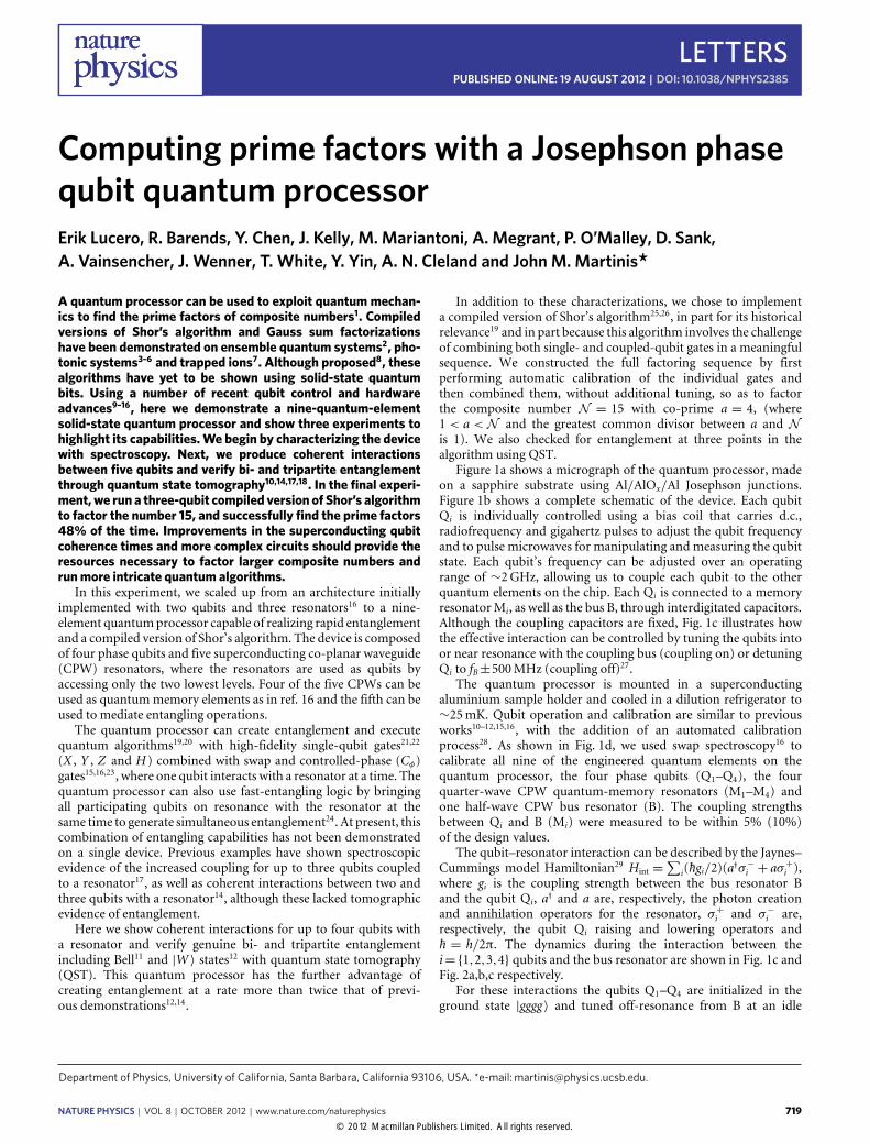
Figure 1a shows a micrograph of the quantum processor, madeon a sapphire substrate using Al/AlOx/Al Josephson junctions.Figure 1b shows a complete schematic of the device. Each qubitQi is individually controlled using a bias coil that carries d.c.,radiofrequency and gigahertz pulses to adjust the qubit frequencyand to pulse microwaves for manipulating andmeasuring the qubitstate. Each qubit’s frequency can be adjusted over an operatingrange of ∼2GHz, allowing us to couple each qubit to the otherquantum elements on the chip. Each Qi is connected to a memoryresonatorMi, as well as the bus B, through interdigitated capacitors.Although the coupling capacitors are fixed, Fig. 1c illustrates howthe effective interaction can be controlled by tuning the qubits intoor near resonance with the coupling bus (coupling on) or detuningQi to fB±500MHz (coupling off)27.

The quantum processor is mounted in a superconductingaluminium sample holder and cooled in a dilution refrigerator to∼25mK. Qubit operation and calibration are similar to previousworks10–12,15,16, with the addition of an automated calibrationprocess28. As shown in Fig. 1d, we used swap spectroscopy16 tocalibrate all nine of the engineered quantum elements on thequantum processor, the four phase qubits (Q1–Q4), the fourquarter-wave CPW quantum-memory resonators (M1–M4) andone half-wave CPW bus resonator (B). The coupling strengthsbetween Qi and B (Mi) were measured to be within 5% (10%)of the design values.

The qubit–resonator interaction can be described by the Jaynes–Cummings model Hamiltonian29 Hint =

∑i(hgi/2)(a

†σ−i + aσ+i ),where gi is the coupling strength between the bus resonator Band the qubit Qi, a† and a are, respectively, the photon creationand annihilation operators for the resonator, σ+i and σ−i are,respectively, the qubit Qi raising and lowering operators andh = h/2π. The dynamics during the interaction between thei={1,2,3,4} qubits and the bus resonator are shown in Fig. 1c andFig. 2a,b,c respectively.

For these interactions the qubits Q1–Q4 are initialized in theground state |gggg 〉 and tuned off-resonance from B at an idle

NATURE PHYSICS | VOL 8 | OCTOBER 2012 | www.nature.com/naturephysics 719

© 2012 Macmillan Publishers Limited. All rights reserved.

LETTERS NATURE PHYSICS DOI: 10.1038/NPHYS2385

Control

SQUID

Q1

Q2

Q2

Q1

Q1

Q1 Q2 Q3 Q4

Q2

Q3

Q4

Q3

Q4

Q31 mm

Q4

M1

M3

B

B

B

B

M4

M2

M2

M1

M1

M2M3 M4

M4

M3

M2M1

M3

M4

λ/2

λ/4

Control

SQUID

RF

Freq

uenc

yFr

eque

ncy

(GH

z)

6.8

6.9

7.2

6.1

0

0.0 1.0

200 0 200 0 200 0 200

Pe

Δ (ns) Δ (ns) Δ (ns) Δ (ns)

a

b

c

d

τ τ τ τ

Figure 1 | Architecture and operation of the quantum processor. a, Photomicrograph of the sample, fabricated with aluminium (coloured) on sapphiresubstrate (dark). b, Schematic of the quantum processor. Each phase qubit Qi is capacitively coupled to the central half-wavelength bus resonator B and aquarter-wavelength memory resonator Mi. The control lines carry gigahertz microwave pulses to produce single-qubit operations. Each Qi is coupled to asuperconducting quantum interference device (SQUID) for single-shot readout. c, Illustration of quantum processor operation. By applying pulses on eachcontrol line, each qubit frequency is tuned in and out of resonance with B (M) to perform entangling (memory) operations. d, Swap spectroscopy16 for allfour qubits. Qubit excited state |e〉 probability Pe (colour scale) versus frequency (vertical axis) and interaction time1τ . The centres of the chevronpatterns gives the frequencies of the resonators B, M1–M4, f=6.1,6.8,7.2,7.1,6.9 GHz, respectively. The oscillation periods give the coupling strengthsbetween Qi and B (Mi), which are all∼=55 MHz (∼=20 MHz).

720 NATURE PHYSICS | VOL 8 | OCTOBER 2012 | www.nature.com/naturephysics

© 2012 Macmillan Publishers Limited. All rights reserved.

NATURE PHYSICS DOI: 10.1038/NPHYS2385 LETTERS

0 20 40 60 80 100

0 20 40 60 80 100

1.0

0.5

0.0

P Q1,

P Q2,

PQ

4, P

b

1.0

0.5

0.0

P Q1,

P Q4, P

b

N = 3

N = 2

50 70 90 110 130

Oscillation frequency (MHz)

4

3

2

1N

Q1

Q1

Q1

Q1

Q2

Q2

Q4

Q4

Q4

Q3

B

B

B

B

1/2

¬1/2

0

|ee⟩

s

0

1/3

d e

f

a

b

ψ

Δ (ns)τ

Δ (ns)τ

0 20 40 60 80 100

1.0

0.5

0.0

Δ (ns)

P Q1,

P Q2,

PQ

3, P

Q4, P

b N = 4c

τ

| ⟩

|gg⟩|ee⟩

|gg⟩

|W⟩

|ggg⟩

|eee⟩

|eee⟩

|ggg⟩

Figure 2 | Rapid entanglement for two to four qubits. a–c, The measured state occupation probabilities PQ1−4 (colour) and Pb (black) for increasingnumber of participating qubits N={2,3,4} versus interaction time1τ . In all cases, B is first prepared in the n= 1 Fock state10 and the participating qubitsare then tuned on resonance with B for the interaction time1τ . The single excitation begins in B, spreads to the participating qubits and then returns to B.These coherent oscillations continue for a time1τ and increase in frequency with each additional qubit. d, Oscillation frequency of Pb for increasingnumbers of participating qubits. The error bars indicate the−3 dB point of the Fourier transformed Pb data. The inset schematics illustrate which qubitsparticipate. The coupling strength increases as gN=

√Ng, plotted as a black line fit to the data, with g= 56.5±0.05 MHz. e,f, The real part of the

reconstructed density matrices from QST. e, Bell singlet |ψs〉= (|ge〉−|eg〉)/√

2 with fidelity FBell=〈ψs|ρBell|ψs〉=0.89±0.01 and EOF=0.70.f, Three-qubit |W〉= (|gge〉+|geg〉+|egg〉)/

√3 with fidelity FW =〈W|ρW|W〉=0.69±0.01. The measured imaginary parts (not shown) are found to be

small, with |Im ρψs |<0.05 (e) and |Im ρW|<0.06 (f), as expected theoretically.

frequency f ∼ 6.6GHz. Q1 is prepared in the excited state |e〉 bya π-pulse. B is then pumped into the first Fock state n= 1 by tuningQ1 on resonance (f ∼ 6.1GHz) for a duration 1/2g1 = τ ∼ 9 ns,long enough to complete an iSWAP operation between Q1 and B,|0〉⊗|eggg 〉→|1〉⊗|gggg 〉 (ref. 10).

The participating qubits are then tuned on resonance (f ∼6.1GHz) and left to interact with B for an interaction time 1τ .Figure 2a–c shows the probabilityPQi ofmeasuring the participatingqubits in the excited state, and the probability Pb of B being in then= 1 Fock state, versus 1τ . At the beginning of the interactionthe excitation is initially concentrated in B (Pb maximum) thenspreads evenly between the participating qubits (Pb minimum) andfinally returns back to B, continuing as a coherent oscillation duringthis interaction time.

When the qubits are simultaneously tuned on resonance withB they interact with an effective coupling strength gN that scaleswith the number N of qubits as

√N (ref. 17), analogous to a single

qubit coupled to a resonator in an n-photon Fock state10. For Nqubits, gN =

√Ng , where g = [1/N (

∑i=1,N g

2i )]

1/2. The oscillationfrequency of Pb for each of the four cases i= {1,2,3,4} is shownin Fig. 2 d. These results are similar to those of refs 17,30, but witha larger number N of qubits interacting with the resonator, we canconfirm the

√N scaling of the coupling strengthwithN . From these

data we find amean value of g =56.5±0.05MHz.By tuning the qubits on resonance for a specific interaction

time τ , corresponding to the first minimum of Pb in Fig. 2a,bwe can generate Bell singlets |ψs〉 = (|ge〉 − |eg 〉)/

√2 and |W 〉

states |W 〉 = (|gge〉+ |geg 〉+ |egg 〉)/√3. Stopping the interaction

at this time (τBell = 6.5 ns and τW = 5.1 ns) leaves the single

excitation evenly distributed among the participating qubits andplaces the qubits in the desired equal superposition state similarto the protocol in ref. 14. We are able to further analyse thesestates using full QST. Figure 2e,f shows the reconstructed densitymatrices from this analysis18. The Bell singlet is formed with fidelityFBell= 〈ψs|ρBell|ψs〉 = 0.89±0.01 and entanglement of formation31

EOF = 0.70. The three-qubit |W 〉 state is formed with fidelityFW =〈W |ρW |W 〉= 0.69±0.01, which satisfies the entanglementwitness inequality FW > 2/3 for three-qubit entanglement32.Generating either of these classes of entangled states (bi- andtripartite) requires only a single entangling operation that is shortrelative to the characteristic time for two-qubit gates (tg ∼ 50 ns).This entanglement protocol has the further advantage that it can bescaled to an arbitrary number of qubits.

The quantum circuit for the compiled version of Shor’salgorithm is shown in Fig. 3a for factoring the number N = 15with a = 4 co-prime25,26, which returns the period r = 2 (10in binary) with a theoretical success rate of 50%. Although thesuccess of the algorithm hinges on quantum entanglement, the finaloutput is ideally a completelymixed state, σm= (1/2)(|0〉〈0|+|1〉〈1|).Therefore, measuring only the raw probabilities of the outputregister does not reveal the underlying quantum entanglementnecessary for the success of the computation. Thus, we perform aruntime analysis with QST at the three points identified in Fig. 3b,in addition to recording the rawprobabilities of the output register.

The first breakpoint in the algorithm verifies the existenceof bipartite entanglement. A Bell singlet |ψs〉 is formed after aHadamard gate22 (H ) onQ2 and a controlled-NOT (CNOT; refs 15,16) between Q2 and Q3. As illustrated in Fig. 3c, the CNOT gates

NATURE PHYSICS | VOL 8 | OCTOBER 2012 | www.nature.com/naturephysics 721

© 2012 Macmillan Publishers Limited. All rights reserved.

LETTERS NATURE PHYSICS DOI: 10.1038/NPHYS2385

QuantumFourier

transform

1/2

0

¬1/2|ee⟩

|0⟩

|ee⟩ |gg⟩|gg⟩

1 | s⟩

HH

HH

H

H

H H

H

H

Cz

Cπ/2

Q2

Q2

Q1

Q2

Q3

Q4

Q3

Q4

Q3

1 2 3

Init Modularexponentiation

armod( ) 00 10

0 1

0 1

0 1

0 1

2

3

|GHz⟩

| 3⟩

0

0

0

0

0

1

1

01

1

1

01

1/2

1

0

1/2

1

0

1/2

1

1/4

1/2

0

0

¬1/4

|eee⟩

|eee⟩

|eee⟩

|eee⟩

|ggg⟩

|ggg⟩

|ggg⟩

|ggg⟩

a

b

c

d

e

f

g

h

i

ψ

ψ

|0⟩

|0⟩

|0⟩

|0⟩

|0⟩

|0⟩

Figure 3 | Compiled version of Shor’s algorithm. a, Four-qubit circuit to factor N = 15, with co-prime a=4. The three steps in the algorithm areinitialization (Init), modular exponentiation and the quantum Fourier transform, which computes armod(N ) and returns the period r= 2. b, Recompiledthree-qubit version of Shor’s algorithm. The redundant qubit Q1 is removed by noting that HH= I. Circuits a and b are equivalent for this specific case. Thethree steps of the runtime analysis are labelled 1,2 and 3. c, CNOT gates are realized using an equivalent CZ circuit. d, Step 1: Bell singlet between Q2 andQ3 with fidelity FBell=〈ψs|ρBell|ψs〉=0.75±0.01 and EOF=0.43. e, Step 2: Three-qubit |GHZ〉= (|ggg〉+|eee〉)/

√2 between Q2, Q3 and Q4 with fidelity

FGHZ=〈GHZ|ρGHZ|GHZ〉=0.59±0.01. f, Step 3: QST after running the complete algorithm. The three-qubit |GHZ〉 is rotated into|ψ3〉=H2|GHZ〉= (|ggg〉+|egg〉+|gee〉−|eee〉)/2 with fidelity F=0.55. g,h, The density matrix of the single-qubit output register Q2 formed by:tracing-out Q3 and Q4 from f (g), and directly measuring Q2 with QST (h), both with F=

√ρ σm√ρ=0.92±0.01 and Sl=0.78. From 1.5× 105 direct

measurements, the output register returns the period r= 2, with probability 0.483±0.003, yielding the prime factors 3 and 5. i, The density matrix of thesingle-qubit output register without entangling gates, H2H2|g〉= I|g〉. Ideally this calibration algorithm returns r=0 100% of the time. Compared with thesingle quantum state |ψout〉= |g〉, the fidelity Fcal=〈ψg|ρcal|ψg〉=0.83±0.01, which is less than unity owing to the energy relaxation.

are processed by inserting a controlled-Z (CZ) between twoH gateson the target qubit. The CZ is realized as in ref. 16 by bringing thetarget qubit |f 〉↔ |e〉 transition on resonance with B to execute an(iSWAP)2. The target qubit acquires a phase shift of π conditionedon the control qubit. Figure 3d is the real part of the density matrixreconstructed from QST on |ψs〉. The singlet is formed with fidelityFBell = 〈ψs|ρBell|ψs〉 = 0.75±0.01 (|Im ρψs |< 0.05 not shown) andEOF= 0.43. The primary cause of the reduced fidelites were energyrelaxation and dephasing of the qubits, with characteristic times ofT1 ∼ 400 ns and T2 ∼ 200 ns, respectively, for all four qubits andT1∼ 3 µs for the bus resonator. Measurement fidelities for |g 〉 and|e〉 for the four qubits are M1,g = 0.9523, M1,e = 0.8902, M2,g =

0.9596,M2,e = 0.9049,M3,g = 0.9490,M3,e = 0.9365,M4,g = 0.9579and M4,e = 0.8323. For all reported QST fidelities, measurementerrors have been subtracted.

The next breakpoint in the algorithm is after the second CNOTgate between Q2 and Q4 to check for tripartite entanglement. Atthis point a three-qubit |GHZ〉 = (|ggg 〉+ |eee〉)/

√2, with fidelity

FGHZ = 〈GHZ|ρGHZ|GHZ〉 = 0.59 ± 0.01 (|Im ρGHZ| < 0.06 notshown), is formed between Q2, Q3 and Q4, as shown in Fig. 3e.This state is found to satisfy the entanglement witness inequalityFGHZ>1/2 (ref. 32), indicating three-qubit entanglement.

The third step in the runtime analysis captures all three qubitsat the end of the algorithm, where the final H gate on Q2 rotates

the three-qubit |GHZ〉 into |ψ3〉 = H2|GHZ〉 = (|ggg 〉 + |egg 〉 +|gee〉 − |eee〉)/2. Figure 3f is the real part of the density matrixwith fidelity F = 〈ψ3|ρ3|ψ3〉 = 0.54± 0.01. From the three-qubitQST we can trace out the register qubit to compare with theexperiment where we measure only the single-qubit register andthe raw probabilities of the algorithm output. Ideally, the algorithmreturns the binary output 00 or 10 (including the redundant qubit)with equal probability, where the former represents a failure andthe latter indicates the successful determination of r = 2. We usethree methods to analyse the output of the algorithm: three-qubitQST, single-qubit QST and the raw probabilities of the outputregister state. Figure 3g,h is the real part of the density matricesfor the single-qubit output register from three-qubit QST andone-qubit QST with fidelity F =

√ρ σm√ρ = 0.92 ± 0.01 for

both density matrices. From the raw probabilities calculated from150,000 repetitions of the algorithm, we measure the output 10with probability 0.483± 0.003, yielding r = 2, and after classicalprocessing we compute the prime factors 3 and 5.

The linear entropy Sl = 4[1−Tr(ρ2)]/3 is another metric forcomparing the observed output to the ideal mixed state, whereSl = 1 for a completely mixed state33. We find Sl = 0.78 for boththe reduced density matrix from the third step of the runtimeanalysis (three-qubit QST), and from direct single-qubit QSTof the register qubit.

722 NATURE PHYSICS | VOL 8 | OCTOBER 2012 | www.nature.com/naturephysics

© 2012 Macmillan Publishers Limited. All rights reserved.

NATURE PHYSICS DOI: 10.1038/NPHYS2385 LETTERSAs an extra calibration to verify that the system possesses

coherence throughout the duration of the algorithm, we removethe entangling operations and use QST to measure the single-qubitoutput register. The circuit reduces to two H gates separated bythe time of the two entangling gates, equivalent to the time ofthe full algorithm. Ideally Q2 returns to the ground state andthe algorithm output is 0 100% of the time. Figure 3i is the realpart of the density matrix for the register qubit after running thiscalibration. The fidelity of measuring the register qubit in |g 〉 isFcal=〈g |ρcal|g 〉=0.83±0.01, indicating that the system is coherentover the algorithm time.

We have implemented a compiled version of Shor’s algorithmon a quantum processor that correctly finds the prime factorsof 15. We showed that the quantum processor can create Bellstates, both classes of three-qubit entanglement and the requisiteentanglement for properly executing Shor’s algorithm. In addition,we produce coherent interactions between four qubits and the busresonator with a protocol that can be scaled to create an N -qubit|W 〉 state, by adding more qubits to the bus resonator. Duringthese coherent interactions, we observe the

√N dependence of

the effective coupling strength with the number N of participatingqubits. These demonstrations represent an important milestonefor superconducting qubits, further proving this architecture forquantum computation and quantum simulations.

Received 25 February 2012; accepted 6 July 2012; published online19 August 2012

References1. Shor, P. Proc. 35th Annual Symp. Foundations of Computer Science 124–134

(IEEE, 1994).2. Vandersypen, L. M. et al. Experimental realization of Shor’s quantum factoring

algorithm using nuclear magnetic resonance. Nature 414, 883–887 (2001).3. Lanyon, B. et al. Experimental Demonstration of a compiled version of Shors

algorithm with quantum entanglement. Phys. Rev. Lett. 99, 250505 (2007).4. Lu, C-Y., Browne, D., Yang, T. & Pan, J-W. Demonstration of a compiled

version of shors quantum factoring algorithm using photonic qubits. Phys.Rev. Lett. 99, 250504 (2007).

5. Politi, A., Matthews, J. C. F. & O’Brien, J. L. Shor’s quantum factoringalgorithm on a photonic chip. Science 325, 1221 (2009).

6. Bigourd, D., Chatel, B., Schleich, W. & Girard, B. Factorization of numberswith the temporal Talbot effect: Optical implementation by a sequence ofshaped ultrashort pulses. Phys. Rev. Lett. 100, 030202 (2008).

7. Gilowski, M. et al. Gauss sum factorization with cold atoms. Phys. Rev. Lett.100, 030201 (2008).

8. Ng, H. & Nori, F. Quantum phase measurement and Gauss sum factorizationof large integers in a superconducting circuit. Phys. Rev. A 82, 042317 (2010).

9. Clarke, J. & Wilhelm, F. K. Superconducting quantum bits. Nature 453,1031–1042 (2008).

10. Hofheinz, M. et al. Generation of Fock states in a superconducting quantumcircuit. Nature 454, 310–314 (2008).

11. Ansmann, M. et al. Violation of Bell’s inequality in Josephson phase qubits.Nature 461, 504–506 (2009).

12. Neeley, M. et al. Generation of three-qubit entangled states usingsuperconducting phase qubits. Nature 467, 570–573 (2010).

13. Dicarlo, L. et al. Preparation and measurement of three-qubit entanglement ina superconducting circuit. Nature 467, 574–578 (2010).

14. Altomare, F. et al. Tripartite interactions between two phase qubits and aresonant cavity. Nature Phys. 6, 777–781 (2010).

15. Yamamoto, T. et al. Quantum process tomography of two-qubit controlled-Zand controlled-NOT gates using superconducting phase qubits. Phys. Rev. B82, 184515 (2010).

16. Mariantoni, M. et al. Implementing the quantum von Neumann architecturewith superconducting circuits. Science 334, 61–65 (2011).

17. Fink, J. et al. Dressed collective qubit states and the Tavis–Cummings Model inCircuit QED. Phys. Rev. Lett. 103, 083601 (2009).

18. Steffen, M. et al. State tomography of capacitively shunted phase qubits withhigh fidelity. Phys. Rev. Lett. 97, 050502 (2006).

19. Nielsen, M. A. & Chuang, I. L. Quantum Computation and QuantumInformation (Cambridge Univ. Press, 2000).

20. Barenco, A. et al. Elementary gates for quantum computation. Phys. Rev. A 52,3457–3467 (1995).

21. Lucero, E. et al. High-fidelity gates in a single Josephson qubit. Phys. Rev. Lett.100, 247001 (2008).

22. Lucero, E. et al. Reduced phase error through optimized control of asuperconducting qubit. Phys. Rev. A 82, 042339 (2010).

23. DiCarlo, L. et al. Demonstration of two-qubit algorithms with asuperconducting quantum processor. Nature 460, 240–244 (2009).

24. Tessier, T., Deutsch, I., Delgado, a. & Fuentes-Guridi, I. Entanglementsharing in the two-atom Tavis-Cummings model. Phys. Rev. A 68,062316 (2003).

25. Beckman, D., Chari, A., Devabhaktuni, S. & Preskill, J. Efficient networks forquantum factoring. Phys. Rev. A 54, 1034–1063 (1996).

26. Buscemi, F. Shors quantum algorithm using electrons in semiconductornanostructures. Phys. Rev. A 83, 012302 (2011).

27. Hofheinz, M. et al. Synthesizing arbitrary quantum states in a superconductingresonator. Nature 459, 546–549 (2009).

28. Lucero, E. Computing prime factors on a Josephson phase-qubitarchitecture:15= 3×5. PhD thesis, Univ. California (2012).

29. Jaynes, E. & Cummings, F. Comparison of quantum and semiclassical radiationtheories with application to the beam maser. Proc. IEEE 51, 89–109 (1963).

30. Mlynek, J. A. et al. Time resolved collective entanglement dynamics in cavityquantum electrodynamics. Preprint at http://arxiv.org/abs/1202.5191 (2012).

31. Hill, S. &Wootters, W. Entanglement of a pair of quantum bits. Phys. Rev. Lett.78, 5022–5025 (1997).

32. Acín, a., Bruß, D., Lewenstein, M. & Sanpera, a. Classification of mixedthree-qubit states. Phys. Rev. Lett. 87, 040401 (2001).

33. White, A. G. et al. Measuring two-qubit gates. J. Opt. Soc. Amer. B 24,172–183 (2007).

AcknowledgementsDevices were made at the UCSB Nanofabrication Facility, a part of the NSF-fundedNational Nanotechnology Infrastructure Network. This work was supported by IARPAunder ARO awards W911NF-08-1-0336 and W911NF-09-1-0375. R.B. acknowledgessupport from the Rubicon program of the Netherlands Organisation for ScientificResearch. M.M. acknowledges support from an Elings Postdoctoral Fellowship.The authors thank S. Ashhab and A. Galiautdinov for useful comments onrapid entanglement.

Author contributionsE.L. fabricated the sample, performed the experiments and analysed the data. E.L. andJ.M.M. designed the custom electronics. E.L., M.M. and D.S. contributed to softwareinfrastructure. All authors contributed to the fabrication process, qubit design,experimental set-up and manuscript preparation.

Additional informationReprints and permissions information is available online at www.nature.com/reprints.Correspondence and requests for materials should be addressed to J.M.M.

Competing financial interestsThe authors declare no competing financial interests.

NATURE PHYSICS | VOL 8 | OCTOBER 2012 | www.nature.com/naturephysics 723

© 2012 Macmillan Publishers Limited. All rights reserved.