Embed Size (px)
Citation preview

Convergence of ABC methods
Christian P. Robert
Universite Paris-Dauphine, University of Warwick, & IUF
joint work with D. Frazier, G. Martin & J. Rousseau

Outline
1 Approximate Bayesian computation
2 [some] asymptotics of ABC
Approximate Bayesian computation
1 Approximate Bayesian computationABC basics
2 [some] asymptotics of ABC
Untractable likelihoods
Cases when the likelihood functionf (y|θ) is unavailable and when thecompletion step
f (y|θ) =
∫Zf (y, z|θ) dz
is impossible or too costly because ofthe dimension of zc© MCMC cannot be implemented!
Untractable likelihoods
Cases when the likelihood functionf (y|θ) is unavailable and when thecompletion step
f (y|θ) =
∫Zf (y, z|θ) dz
is impossible or too costly because ofthe dimension of zc© MCMC cannot be implemented!
Illustration
Example (Ising & Potts models)
Potts model: if y takes values on a grid Y of size kn and
f (y|θ) ∝ exp
{θ∑l∼i
Iyl=yi
}
where l∼i denotes a neighbourhood relation, n moderately largeprohibits the computation of the normalising constant Zθ
Special case of the intractable normalising constant, making thelikelihood impossible to compute
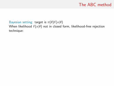
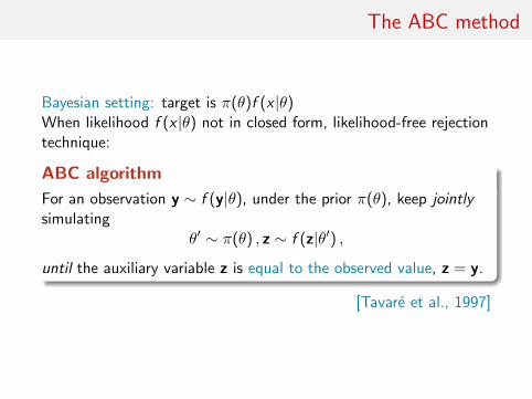
The ABC method
Bayesian setting: target is π(θ)f (x |θ)
When likelihood f (x |θ) not in closed form, likelihood-free rejectiontechnique:
ABC algorithm
For an observation y ∼ f (y|θ), under the prior π(θ), keep jointlysimulating
θ′ ∼ π(θ) , z ∼ f (z|θ′) ,
until the auxiliary variable z is equal to the observed value, z = y.
[Tavare et al., 1997]
The ABC method
Bayesian setting: target is π(θ)f (x |θ)When likelihood f (x |θ) not in closed form, likelihood-free rejectiontechnique:
ABC algorithm
For an observation y ∼ f (y|θ), under the prior π(θ), keep jointlysimulating
θ′ ∼ π(θ) , z ∼ f (z|θ′) ,
until the auxiliary variable z is equal to the observed value, z = y.
[Tavare et al., 1997]
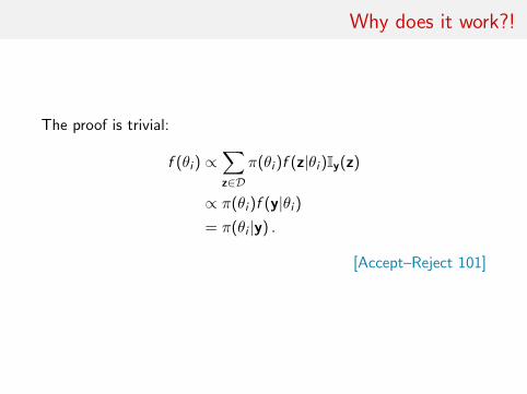
Why does it work?!
The proof is trivial:
f (θi ) ∝∑z∈D
π(θi )f (z|θi )Iy(z)
∝ π(θi )f (y|θi )= π(θi |y) .
[Accept–Reject 101]
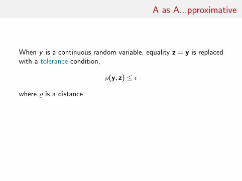
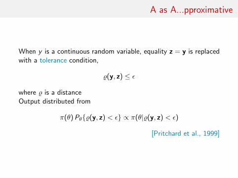
A as A...pproximative
When y is a continuous random variable, equality z = y is replacedwith a tolerance condition,
%(y, z) ≤ ε
where % is a distance
Output distributed from
π(θ)Pθ{%(y, z) < ε} ∝ π(θ|%(y, z) < ε)
[Pritchard et al., 1999]
A as A...pproximative
When y is a continuous random variable, equality z = y is replacedwith a tolerance condition,
%(y, z) ≤ ε
where % is a distanceOutput distributed from
π(θ)Pθ{%(y, z) < ε} ∝ π(θ|%(y, z) < ε)
[Pritchard et al., 1999]
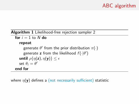
ABC algorithm
Algorithm 1 Likelihood-free rejection sampler 2
for i = 1 to N dorepeat
generate θ′ from the prior distribution π(·)generate z from the likelihood f (·|θ′)
until ρ{η(z), η(y)} ≤ εset θi = θ′
end for
where η(y) defines a (not necessarily sufficient) statistic
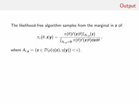
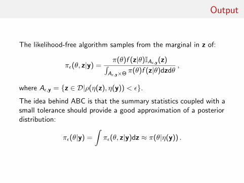
Output
The likelihood-free algorithm samples from the marginal in z of:
πε(θ, z|y) =π(θ)f (z|θ)IAε,y (z)∫
Aε,y×Θ π(θ)f (z|θ)dzdθ,
where Aε,y = {z ∈ D|ρ(η(z), η(y)) < ε}.
The idea behind ABC is that the summary statistics coupled with asmall tolerance should provide a good approximation of a posteriordistribution:
πε(θ|y) =
∫πε(θ, z|y)dz ≈ π(θ|η(y)) .
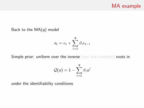
MA example
Back to the MA(q) model
xt = εt +
q∑i=1
ϑiεt−i
Simple prior: uniform over the inverse [real and complex] roots in
Q(u) = 1−q∑
i=1
ϑiui
under the identifiability conditions
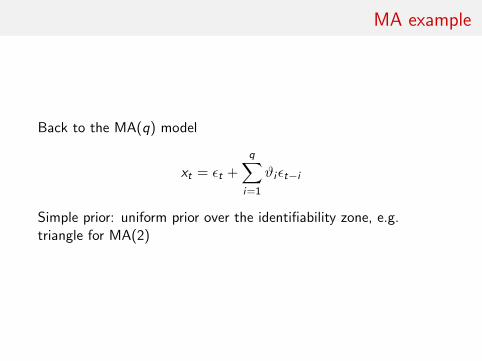
MA example
Back to the MA(q) model
xt = εt +
q∑i=1
ϑiεt−i
Simple prior: uniform prior over the identifiability zone, e.g.triangle for MA(2)
MA example (2)
ABC algorithm thus made of
1 picking a new value (ϑ1, ϑ2) in the triangle
2 generating an iid sequence (εt)−q<t≤T
3 producing a simulated series (x ′t)1≤t≤T
Distance: basic distance between the series
ρ((x ′t)1≤t≤T , (xt)1≤t≤T ) =T∑t=1
(xt − x ′t)2
or distance between summary statistics like the q autocorrelations
τj =T∑
t=j+1
xtxt−j
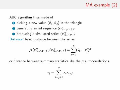
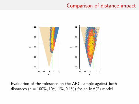
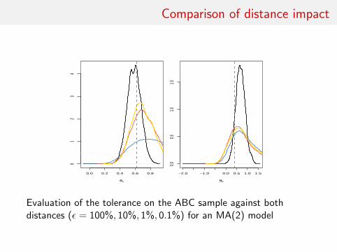
Comparison of distance impact
Evaluation of the tolerance on the ABC sample against bothdistances (ε = 100%, 10%, 1%, 0.1%) for an MA(2) model
Comparison of distance impact
0.0 0.2 0.4 0.6 0.8
01
23
4
θ1
−2.0 −1.0 0.0 0.5 1.0 1.50.0
0.51.0
1.5
θ2
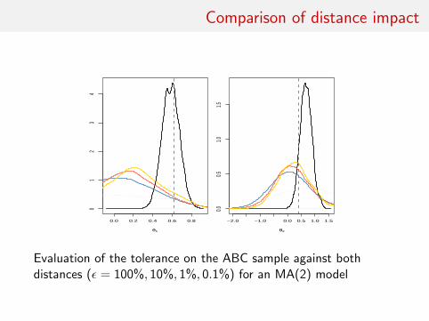
Evaluation of the tolerance on the ABC sample against bothdistances (ε = 100%, 10%, 1%, 0.1%) for an MA(2) model
Comparison of distance impact
0.0 0.2 0.4 0.6 0.8
01
23
4
θ1
−2.0 −1.0 0.0 0.5 1.0 1.50.0
0.51.0
1.5
θ2
Evaluation of the tolerance on the ABC sample against bothdistances (ε = 100%, 10%, 1%, 0.1%) for an MA(2) model
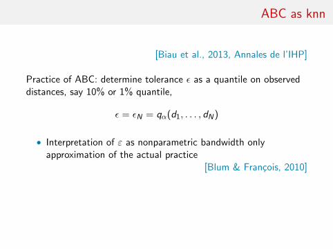
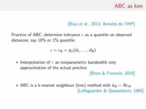
ABC as knn
[Biau et al., 2013, Annales de l’IHP]
Practice of ABC: determine tolerance ε as a quantile on observeddistances, say 10% or 1% quantile,
ε = εN = qα(d1, . . . , dN)
• Interpretation of ε as nonparametric bandwidth onlyapproximation of the actual practice
[Blum & Francois, 2010]
• ABC is a k-nearest neighbour (knn) method with kN = NεN[Loftsgaarden & Quesenberry, 1965]
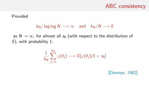
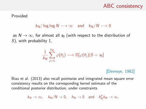
ABC consistency
Provided
kN/ log logN −→∞ and kN/N −→ 0
as N →∞, for almost all s0 (with respect to the distribution ofS), with probability 1,
1
kN
kN∑j=1
ϕ(θj) −→ E[ϕ(θj)|S = s0]
[Devroye, 1982]
Biau et al. (2013) also recall pointwise and integrated mean square errorconsistency results on the corresponding kernel estimate of theconditional posterior distribution, under constraints
kN →∞, kN/N → 0, hN → 0 and hpNkN →∞,
Rates of convergence
Further assumptions (on target and kernel) allow for precise(integrated mean square) convergence rates (as a power of thesample size N), derived from classical k-nearest neighbourregression, like
• when m = 1, 2, 3, kN ≈ N(p+4)/(p+8) and rate N−4
p+8
• when m = 4, kN ≈ N(p+4)/(p+8) and rate N−4
p+8 logN
• when m > 4, kN ≈ N(p+4)/(m+p+4) and rate N−4
m+p+4
[Biau et al., 2013]
Drag: Only applies to sufficient summary statistics
[some] asymptotics of ABC
1 Approximate Bayesian computation
2 [some] asymptotics of ABCasymptotic setupconsistency of ABC posteriorsasymptotic shape of posteriordistributionasymptotic behaviour of EABC [θ]
asymptotic setup
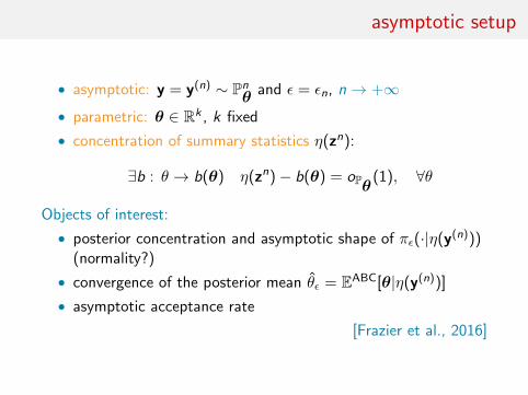
• asymptotic: y = y(n) ∼ Pnθ and ε = εn, n→ +∞
• parametric: θ ∈ Rk , k fixed
• concentration of summary statistics η(zn):
∃b : θ → b(θ) η(zn)− b(θ) = oPθ(1), ∀θ
Objects of interest:
• posterior concentration and asymptotic shape of πε(·|η(y(n)))(normality?)
• convergence of the posterior mean θε = EABC[θ|η(y(n))]
• asymptotic acceptance rate
[Frazier et al., 2016]
asymptotic setup
• asymptotic: y = y(n) ∼ Pnθ and ε = εn, n→ +∞
• parametric: θ ∈ Rk , k fixed
• concentration of summary statistics η(zn):
∃b : θ → b(θ) η(zn)− b(θ) = oPθ(1), ∀θ
Objects of interest:
• posterior concentration and asymptotic shape of πε(·|η(y(n)))(normality?)
• convergence of the posterior mean θε = EABC[θ|η(y(n))]
• asymptotic acceptance rate
[Frazier et al., 2016]
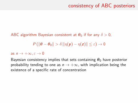
consistency of ABC posteriors
ABC algorithm Bayesian consistent at θ0 if for any δ > 0,
P (‖θ − θ0‖ > δ|‖η(y)− η(z)‖ ≤ ε)→ 0
as n→ +∞, ε→ 0
Bayesian consistency implies that sets containing θ0 have posteriorprobability tending to one as n→ +∞, with implication being theexistence of a specific rate of concentration
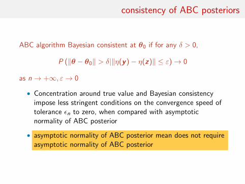
consistency of ABC posteriors
ABC algorithm Bayesian consistent at θ0 if for any δ > 0,
P (‖θ − θ0‖ > δ|‖η(y)− η(z)‖ ≤ ε)→ 0
as n→ +∞, ε→ 0
• Concentration around true value and Bayesian consistencyimpose less stringent conditions on the convergence speed oftolerance εn to zero, when compared with asymptoticnormality of ABC posterior
• asymptotic normality of ABC posterior mean does not requireasymptotic normality of ABC posterior
consistency of ABC posteriors
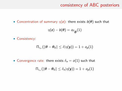
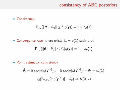
• Concentration of summary η(z): there exists b(θ) such that
η(z)− b(θ) = oPθ(1)
• Consistency:
Πεn (‖θ − θ0‖ ≤ δ|η(y)) = 1 + op(1)
• Convergence rate: there exists δn = o(1) such that
Πεn (‖θ − θ0‖ ≤ δn|η(y)) = 1 + op(1)
consistency of ABC posteriors
• Consistency:
Πεn (‖θ − θ0‖ ≤ δ|η(y)) = 1 + op(1)
• Convergence rate: there exists δn = o(1) such that
Πεn (‖θ − θ0‖ ≤ δn|η(y)) = 1 + op(1)
• Point estimator consistency
θε = EABC [θ|η(y(n))], EABC [θ|η(y(n))]− θ0 = op(1)
vn(EABC [θ|η(y(n))]− θ0)⇒ N(0, v)
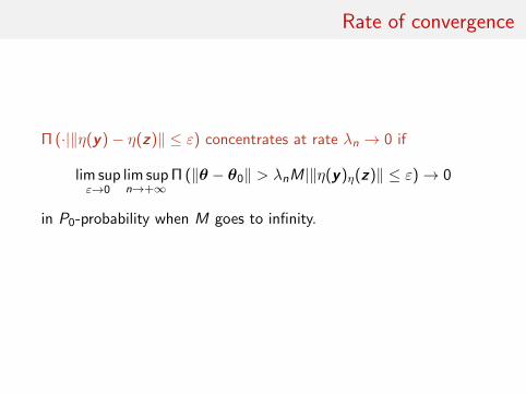
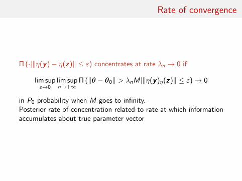
Rate of convergence
Π (·|‖η(y)− η(z)‖ ≤ ε) concentrates at rate λn → 0 if
lim supε→0
lim supn→+∞
Π (‖θ − θ0‖ > λnM|‖η(y)η(z)‖ ≤ ε)→ 0
in P0-probability when M goes to infinity.
Posterior rate of concentration related to rate at which informationaccumulates about true parameter vector
Rate of convergence
Π (·|‖η(y)− η(z)‖ ≤ ε) concentrates at rate λn → 0 if
lim supε→0
lim supn→+∞
Π (‖θ − θ0‖ > λnM|‖η(y)η(z)‖ ≤ ε)→ 0
in P0-probability when M goes to infinity.Posterior rate of concentration related to rate at which informationaccumulates about true parameter vector
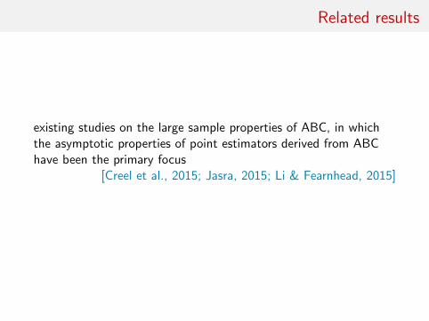
Related results
existing studies on the large sample properties of ABC, in whichthe asymptotic properties of point estimators derived from ABChave been the primary focus
[Creel et al., 2015; Jasra, 2015; Li & Fearnhead, 2015]
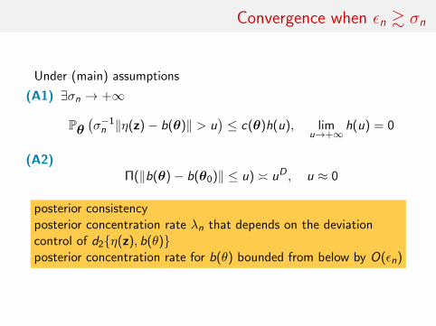
Convergence when εn & σn
Under (main) assumptions
(A1) ∃σn → +∞
Pθ(σ−1n ‖η(z)− b(θ)‖ > u
)≤ c(θ)h(u), lim
u→+∞h(u) = 0
(A2)Π(‖b(θ)− b(θ0)‖ ≤ u) � uD , u ≈ 0
posterior consistencyposterior concentration rate λn that depends on the deviationcontrol of d2{η(z), b(θ)}posterior concentration rate for b(θ) bounded from below by O(εn)
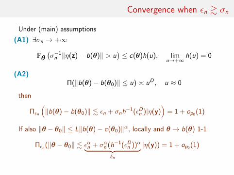
Convergence when εn & σn
Under (main) assumptions
(A1) ∃σn → +∞
Pθ(σ−1n ‖η(z)− b(θ)‖ > u
)≤ c(θ)h(u), lim
u→+∞h(u) = 0
(A2)Π(‖b(θ)− b(θ0)‖ ≤ u) � uD , u ≈ 0
then
Πεn
(‖b(θ)− b(θ0)‖ . εn + σnh
−1(εDn )|η(y))
= 1 + op0(1)
If also ‖θ − θ0‖ ≤ L‖b(θ)− c(θ0)‖α, locally and θ → b(θ) 1-1
Πεn(‖θ − θ0‖ . εαn + σαn (h−1(εDn ))α︸ ︷︷ ︸δn
|η(y)) = 1 + op0(1)
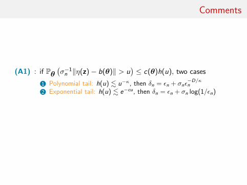
Comments
(A1) : if Pθ(σ−1n ‖η(z)− b(θ)‖ > u
)≤ c(θ)h(u), two cases
1 Polynomial tail: h(u) . u−κ, then δn = εn + σnε−D/κn
2 Exponential tail: h(u) . e−cu, then δn = εn + σn log(1/εn)
• E.g., η(y) = n−1∑
i g(yi ) with moments on g (case 1) orLaplace transform (case 2)
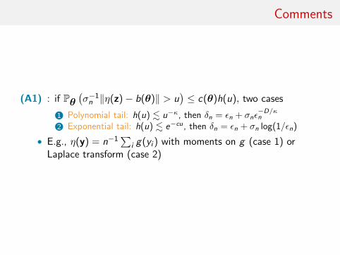
Comments
(A1) : if Pθ(σ−1n ‖η(z)− b(θ)‖ > u
)≤ c(θ)h(u), two cases
1 Polynomial tail: h(u) . u−κ, then δn = εn + σnε−D/κn
2 Exponential tail: h(u) . e−cu, then δn = εn + σn log(1/εn)
• E.g., η(y) = n−1∑
i g(yi ) with moments on g (case 1) orLaplace transform (case 2)
Comments
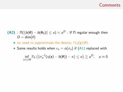
(A2) : Π(‖b(θ)− b(θ0)‖ ≤ u) � uD : If Π regular enough thenD = dim(θ)
• no need to approximate the density f (η(y)|θ).
• Same results holds when εn = o(σn) if (A1) replaced with
inf|x |≤M
Pθ(‖σ−1
n (η(z)− b(θ))− x‖ ≤ u)& uD , u ≈ 0
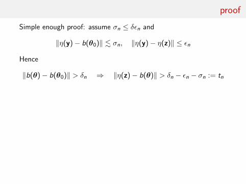
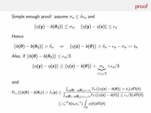
proof
Simple enough proof: assume σn ≤ δεn and
‖η(y)− b(θ0)‖ . σn, ‖η(y)− η(z)‖ ≤ εn
Hence
‖b(θ)− b(θ0)‖ > δn ⇒ ‖η(z)− b(θ)‖ > δn − εn − σn := tn
Also, if ‖b(θ)− b(θ0)‖ ≤ εn/3
‖η(y)− η(z)‖ ≤ ‖η(z)− b(θ)‖+ σn︸︷︷︸≤εn/3
+εn/3
and
Πεn (‖b(θ)− b(θ0)‖ > δn|y) ≤
∫‖b(θ)−b(θ0)‖>δn
Pθ (‖η(z)− b(θ)‖ > tn) dΠ(θ)∫|b(θ)−b(θ0)|≤εn/3
Pθ (‖η(z)− b(θ)‖ ≤ εn/3) dΠ(θ)
. ε−Dn h(tnσ
−1n )
∫Θ
c(θ)dΠ(θ)
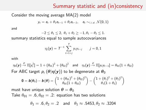
Summary statistic and (in)consistency
Consider the moving average MA(2) model
yt = et + θ1et−1 + θ2et−2, et ∼i.i.d. N (0, 1)
and−2 ≤ θ1 ≤ 2, θ1 + θ2 ≥ −1, θ1 − θ2 ≤ 1.
summary statistics equal to sample autocovariances
ηj(y) = T−1T∑
t=1+j
ytyt−j j = 0, 1
with
η0(y)P→ E[y 2
t ] = 1 + (θ01)2 + (θ02)2 and η1(y)P→ E[ytyt−1] = θ01(1 + θ02)
For ABC target pε (θ|η(y)) to be degenerate at θ0
0 = b(θ0)− b (θ) =
(1 + (θ01)2 + (θ02)2
θ01(1 + θ02)
)−(
1 + (θ1)2 + (θ2)2
θ1(1 + θ2)
)must have unique solution θ = θ0
Take θ01 = .6, θ02 = .2: equation has two solutions
θ1 = .6, θ2 = .2 and θ1 ≈ .5453, θ2 ≈ .3204
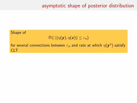
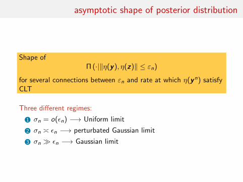
asymptotic shape of posterior distribution
Shape ofΠ (·|‖η(y), η(z)‖ ≤ εn)
for several connections between εn and rate at which η(yn) satisfyCLT
Three different regimes:
1 σn = o(εn) −→ Uniform limit
2 σn � εn −→ perturbated Gaussian limit
3 σn � εn −→ Gaussian limit
asymptotic shape of posterior distribution
Shape ofΠ (·|‖η(y), η(z)‖ ≤ εn)
for several connections between εn and rate at which η(yn) satisfyCLT
Three different regimes:
1 σn = o(εn) −→ Uniform limit
2 σn � εn −→ perturbated Gaussian limit
3 σn � εn −→ Gaussian limit
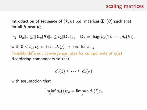
scaling matrices
Introduction of sequence of (k, k) p.d. matrices Σn(θ) such thatfor all θ near θ0
c1‖Dn‖∗ ≤ ‖Σn(θ)‖∗ ≤ c2‖Dn‖∗, Dn = diag(dn(1), · · · , dn(k)),
with 0 < c1, c2 < +∞, dn(j)→ +∞ for all j
Possibly different convergence rates for components of η(z)Reordering components so that
dn(1) ≤ · · · ≤ dn(k)
with assumption that
lim infn
dn(j)εn = lim supn
dn(j)εn
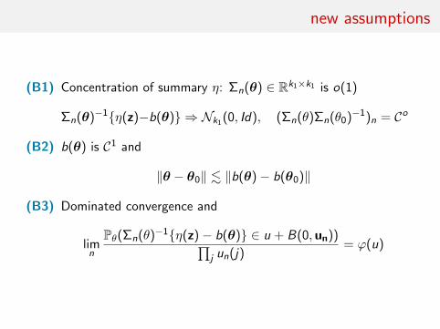
new assumptions
(B1) Concentration of summary η: Σn(θ) ∈ Rk1×k1 is o(1)
Σn(θ)−1{η(z)−b(θ)} ⇒ Nk1(0, Id), (Σn(θ)Σn(θ0)−1)n = Co
(B2) b(θ) is C1 and
‖θ − θ0‖ . ‖b(θ)− b(θ0)‖
(B3) Dominated convergence and
limn
Pθ(Σn(θ)−1{η(z)− b(θ)} ∈ u + B(0,un))∏j un(j)
= ϕ(u)
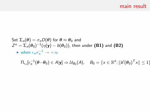
main result
Set Σn(θ) = σnD(θ) for θ ≈ θ0 andZ o = Σn(θ0)−1(η(y)− b(θ0)), then under (B1) and (B2)
• when εnσ−1n → +∞
Πεn [ε−1n (θ−θ0) ∈ A|y]⇒ UB0(A), B0 = {x ∈ Rk ; ‖b′(θ0)T x‖ ≤ 1}
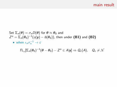
main result
Set Σn(θ) = σnD(θ) for θ ≈ θ0 andZ o = Σn(θ0)−1(η(y)− b(θ0)), then under (B1) and (B2)
• when εnσ−1n → c
Πεn [Σn(θ0)−1(θ − θ0)− Z o ∈ A|y]⇒ Qc(A), Qc 6= N
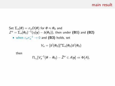
main result
Set Σn(θ) = σnD(θ) for θ ≈ θ0 andZ o = Σn(θ0)−1(η(y)− b(θ0)), then under (B1) and (B2)
• when εnσ−1n → 0 and (B3) holds, set
Vn = [b′(θ0)]nΣn(θ0)b′(θ0)
thenΠεn [V−1
n (θ − θ0)− Z o ∈ A|y]⇒ Φ(A),
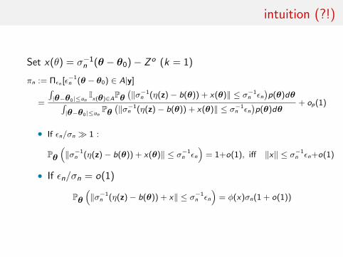
intuition (?!)
Set x(θ) = σ−1n (θ − θ0)− Z o (k = 1)
πn := Πεn [ε−1n (θ − θ0) ∈ A|y]
=
∫|θ−θ0|≤un
Ix(θ)∈APθ
(‖σ−1
n (η(z)− b(θ)) + x(θ)‖ ≤ σ−1n εn
)p(θ)dθ∫
|θ−θ0|≤unPθ(‖σ−1
n (η(z)− b(θ)) + x(θ)‖ ≤ σ−1n εn
)p(θ)dθ
+ op(1)
• If εn/σn � 1 :
Pθ(‖σ−1
n (η(z)− b(θ)) + x(θ)‖ ≤ σ−1n εn
)= 1+o(1), iff ‖x‖ ≤ σ−1
n εn+o(1)
• If εn/σn = o(1)
Pθ(‖σ−1
n (η(z)− b(θ)) + x‖ ≤ σ−1n εn
)= φ(x)σn(1 + o(1))
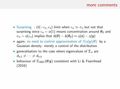
more comments
• Surprising : U(−εn, εn) limit when εn � σn
but not thatsurprising since εn = o(1) means concentration around θ0 andσn = o(εn) implies that b(θ)− b(θ0) ≈ η(z)− η(y)
• again, no need to control approximation of f (η(y)|θ) by aGaussian density: merely a control of the distribution
• generalisation to the case where eigenvalues of Σn aredn,1 6= · · · 6= dn,k
• behaviour of EABC (θ|y) consistent with Li & Fearnhead(2016)
more comments
• Surprising : U(−εn, εn) limit when εn � σn but not thatsurprising since εn = o(1) means concentration around θ0 andσn = o(εn) implies that b(θ)− b(θ0) ≈ η(z)− η(y)
• again, no need to control approximation of f (η(y)|θ) by aGaussian density: merely a control of the distribution
• generalisation to the case where eigenvalues of Σn aredn,1 6= · · · 6= dn,k
• behaviour of EABC (θ|y) consistent with Li & Fearnhead(2016)
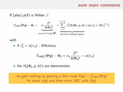
even more comments
If (also) p(θ) is Holder β
EABC (θ|y)− θ0 = σnZ o
b(θ0)′︸ ︷︷ ︸score for f (η(y)|θ)
+
bβ/2c∑j=1
ε2jn Hj(θ0, p, b)
︸ ︷︷ ︸bias from threshold approx
+o(σn) + O(εβ+1n )
with
• if ε2n = o(σn) : Efficiency
EABC (θ|y)− θ0 = σnZ o
b(θ0)′+ o(σn)
• the Hj(θ0, p, b)’s are deterministic
we gain nothing by getting a first crude θ(y) = EABC (θ|y)for some η(y) and then rerun ABC with θ(y)
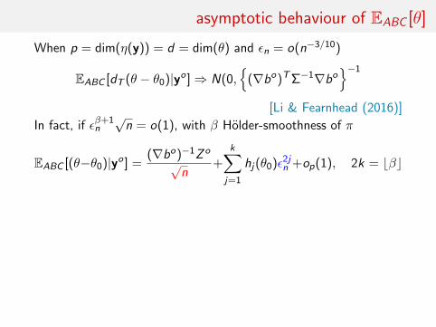
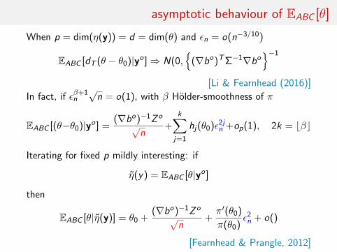
asymptotic behaviour of EABC [θ]
When p = dim(η(y)) = d = dim(θ) and εn = o(n−3/10)
EABC [dT (θ − θ0)|yo ]⇒ N(0,{
(∇bo)TΣ−1∇bo}−1
[Li & Fearnhead (2016)]
In fact, if εβ+1n√n = o(1), with β Holder-smoothness of π
EABC [(θ−θ0)|yo ] =(∇bo)−1Z o
√n
+k∑
j=1
hj(θ0)ε2jn +op(1), 2k = bβc
Iterating for fixed p mildly interesting: if
η(y) = EABC [θ|yo ]
then
EABC [θ|η(y)] = θ0 +(∇bo)−1Z o
√n
+π′(θ0)
π(θ0)ε2n + o()
[Fearnhead & Prangle, 2012]
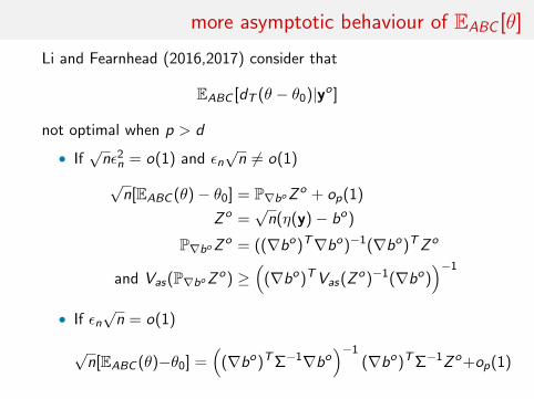
more asymptotic behaviour of EABC [θ]
Li and Fearnhead (2016,2017) consider that
EABC [dT (θ − θ0)|yo ]
not optimal when p > d
• If√nε2
n = o(1) and εn√n 6= o(1)
√n[EABC (θ)− θ0] = P∇boZ o + op(1)
Z o =√n(η(y)− bo)
P∇boZ o = ((∇bo)T∇bo)−1(∇bo)TZ o
and Vas(P∇boZ o) ≥(
(∇bo)TVas(Z o)−1(∇bo))−1
• If εn√n = o(1)
√n[EABC (θ)−θ0] =
((∇bo)TΣ−1∇bo
)−1(∇bo)TΣ−1Z o+op(1)
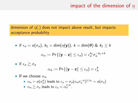
impact of the dimension of η
dimension of η(.) does not impact above result, but impactsacceptance probability
• if εn = o(σn), k1 = dim(η(y)), k = dim(θ) & k1 ≥ k
αn := Pr (‖y − z‖ ≤ εn) � εk1n σ−k1+kn
• if εn & σnαn := Pr (‖y − z‖ ≤ εn) � εkn
• If we choose αn
• αn = o(σkn ) leads to εn = σn(αnσ
−kn )1/k1 = o(σn)
• αn & σn leads to εn � α1/kn .
conclusion on ABC consistency
• asymptotic description of ABC: different regimes dependingon εn & σn
• no point in choosing εn arbitrarily small: just εn = o(σn)
• no asymptotic gain in iterative ABC
• results under weak conditions by not studying g(η(z)|θ)