Embed Size (px)
Citation preview

Machine Learning in High Energy Physics
Lectures 3 & 4
Alex Rogozhnikov
Lund, MLHEP 2016
1 / 99
Recapitulationclassification, regressionkNN classifier and regressorROC curve, ROC AUC
1 / 99
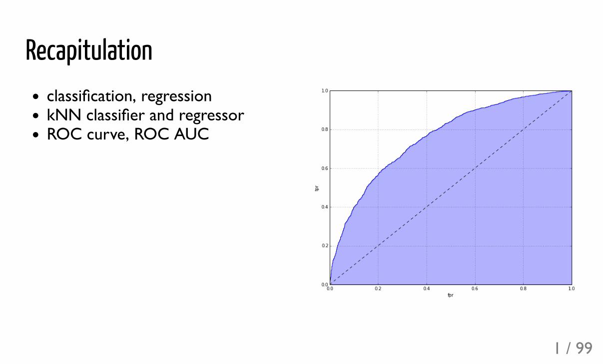
Bayes optimal classifierGiven exact distributions' density functions, we can build an optimal classifier
Need to estimate ratio of likelihoods.
= ×p(y = 1 | x)p(y = 0 | x)
p(y = 1)p(y = 0)
p(x | y = 1)p(x | y = 0)
2 / 99
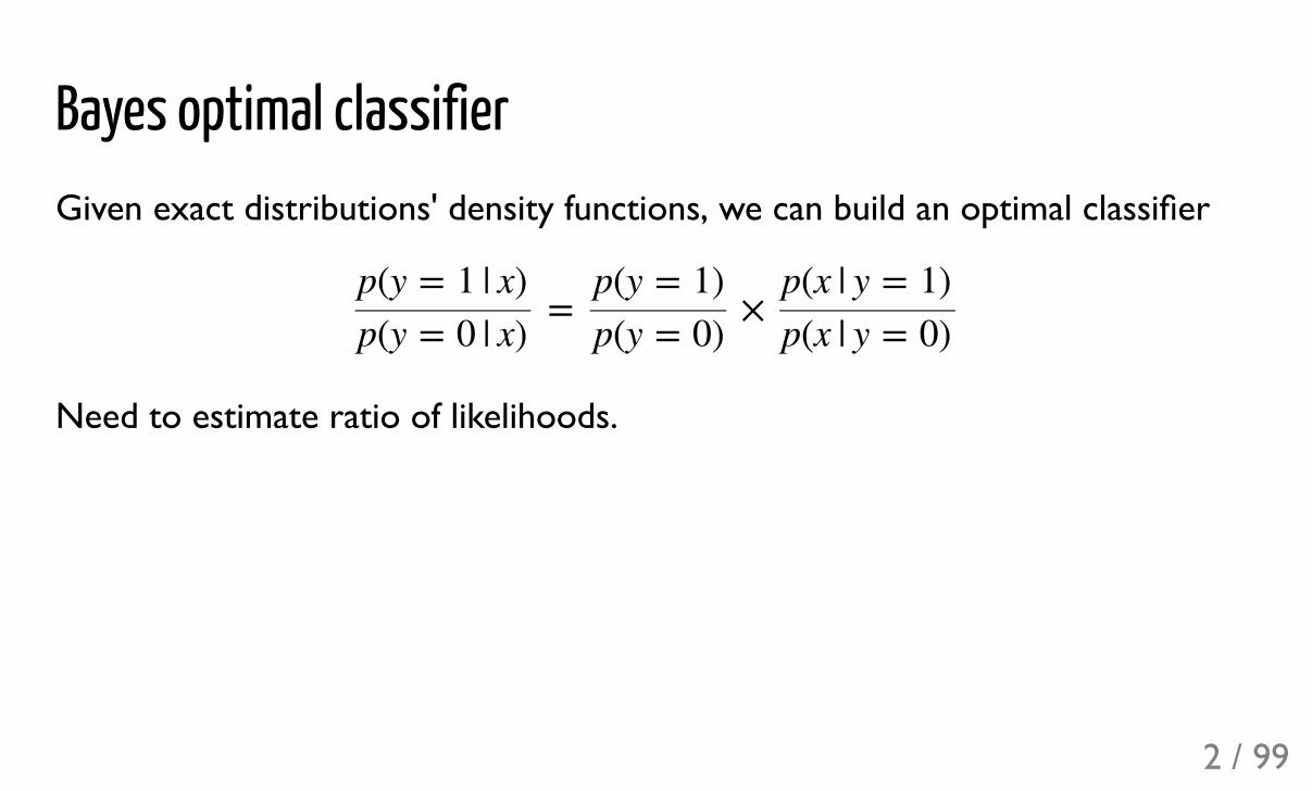
Density estimationHistogramsKernel density estimation
3 / 99
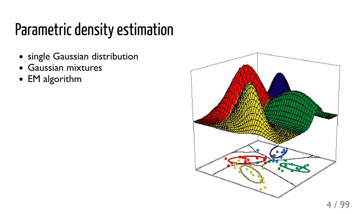
Parametric density estimationsingle Gaussian distributionGaussian mixturesEM algorithm
4 / 99
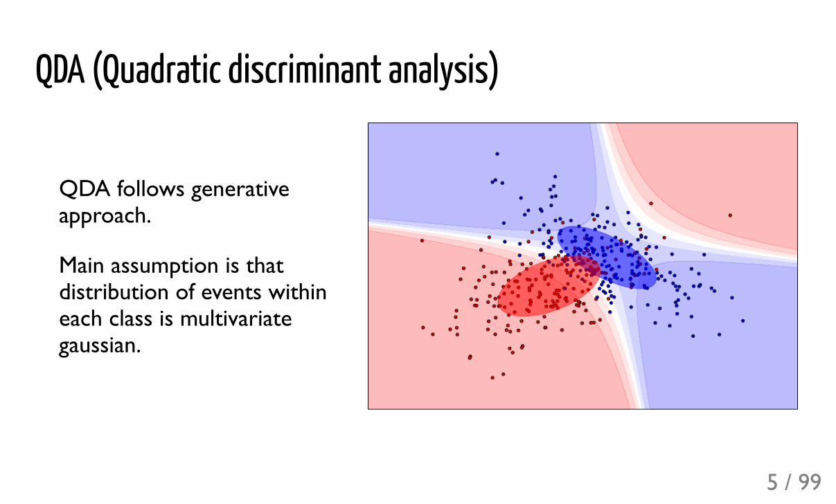
QDA (Quadratic discriminant analysis)
QDA follows generativeapproach.
Main assumption is thatdistribution of events withineach class is multivariategaussian.
5 / 99
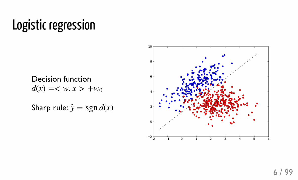
Logistic regression
Decision function
Sharp rule:
d(x) =< w, x > +w0
= sgn d(x)y
6 / 99
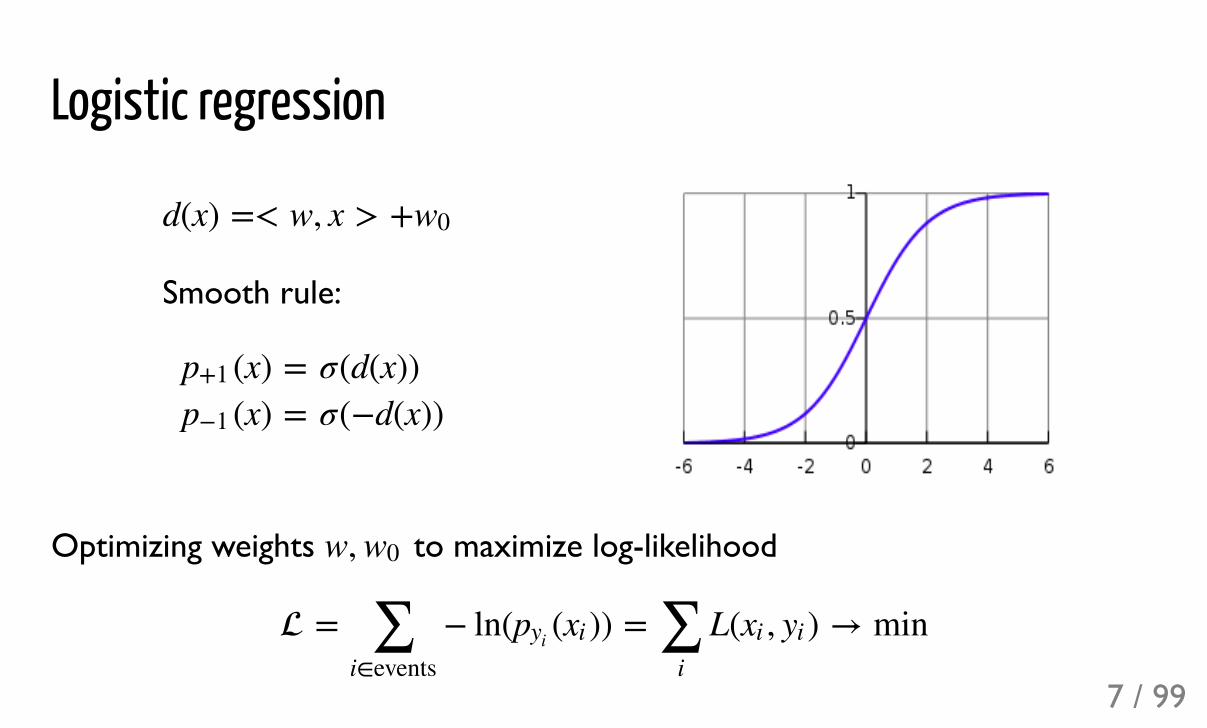
Logistic regression
Smooth rule:
Optimizing weights to maximize log-likelihood
d(x) =< w, x > +w0
(x)p+1
(x)p+1
==σ(d(x))σ(+d(x))
w, w0
= + ln( ( )) = L( , ) → min∑i!events
pyi xi ∑i
xi yi
7 / 99
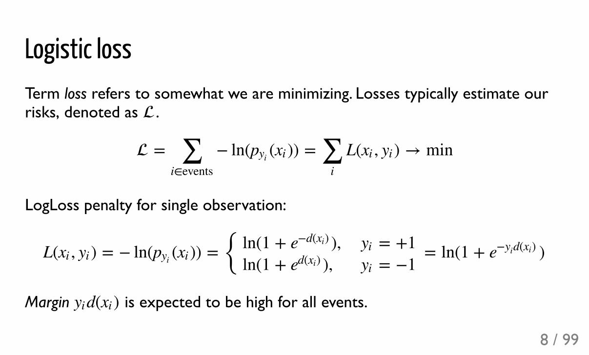
Logistic lossTerm loss refers to somewhat we are minimizing. Losses typically estimate ourrisks, denoted as .
LogLoss penalty for single observation:
Margin is expected to be high for all events.
= + ln( ( )) = L( , ) → min∑i!events
pyi xi ∑i
xi yi
L( , ) = + ln( ( )) = { = ln(1 + )xi yi pyi xiln(1 + ),e+d( )xi
ln(1 + ),ed( )xi
= +1yi
= +1yie+ d( )yi xi
d( )yi xi
8 / 99
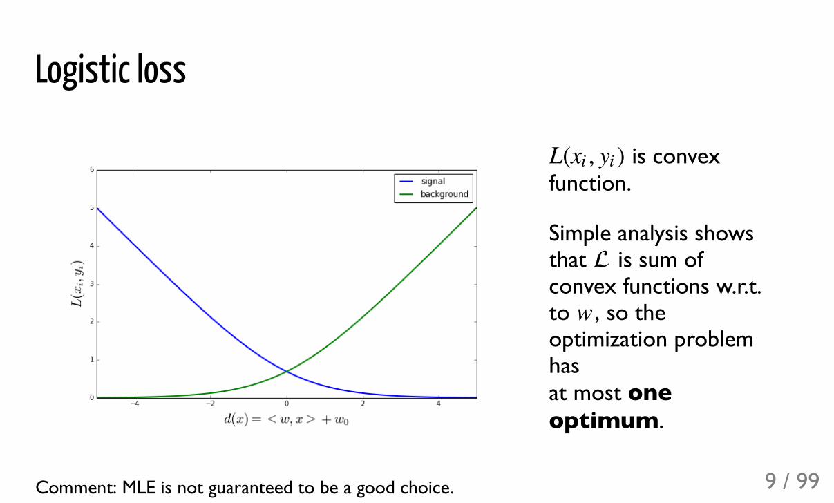
Logistic loss
is convexfunction.
Simple analysis showsthat is sum ofconvex functions w.r.t.to , so theoptimization problemhas at most oneoptimum.
Comment: MLE is not guaranteed to be a good choice.
L( , )xi yi
w
9 / 99
Visualization of logistic regression
10 / 99
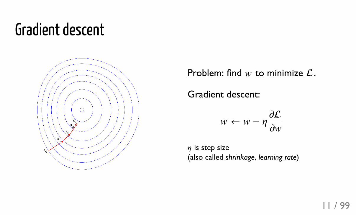
Gradient descent
Problem: find to minimize .
Gradient descent:
is step size (also called shrinkage, learning rate)
w
w ← w + η��w
η
11 / 99
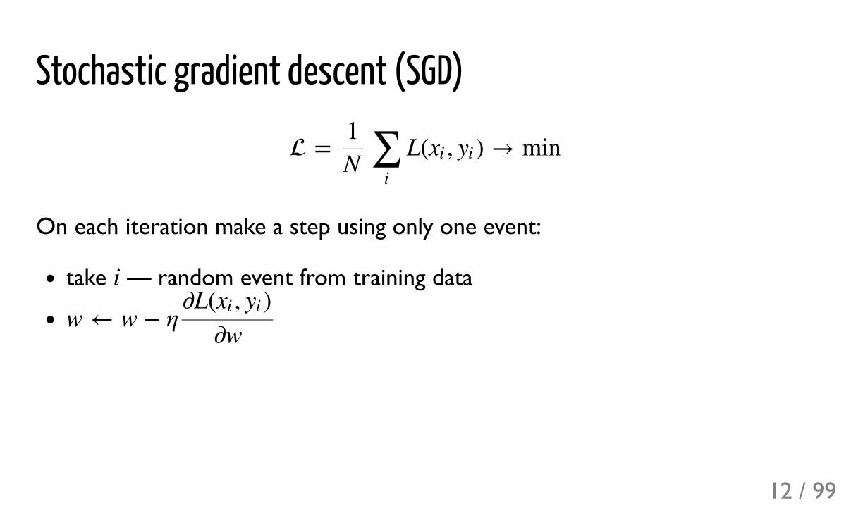
Stochastic gradient descent (SGD)
On each iteration make a step using only one event:
take — random event from training data
= L( , ) → min1N ∑
i
xi yi
i
w ← w + η�L( , )xi yi
�w
12 / 99
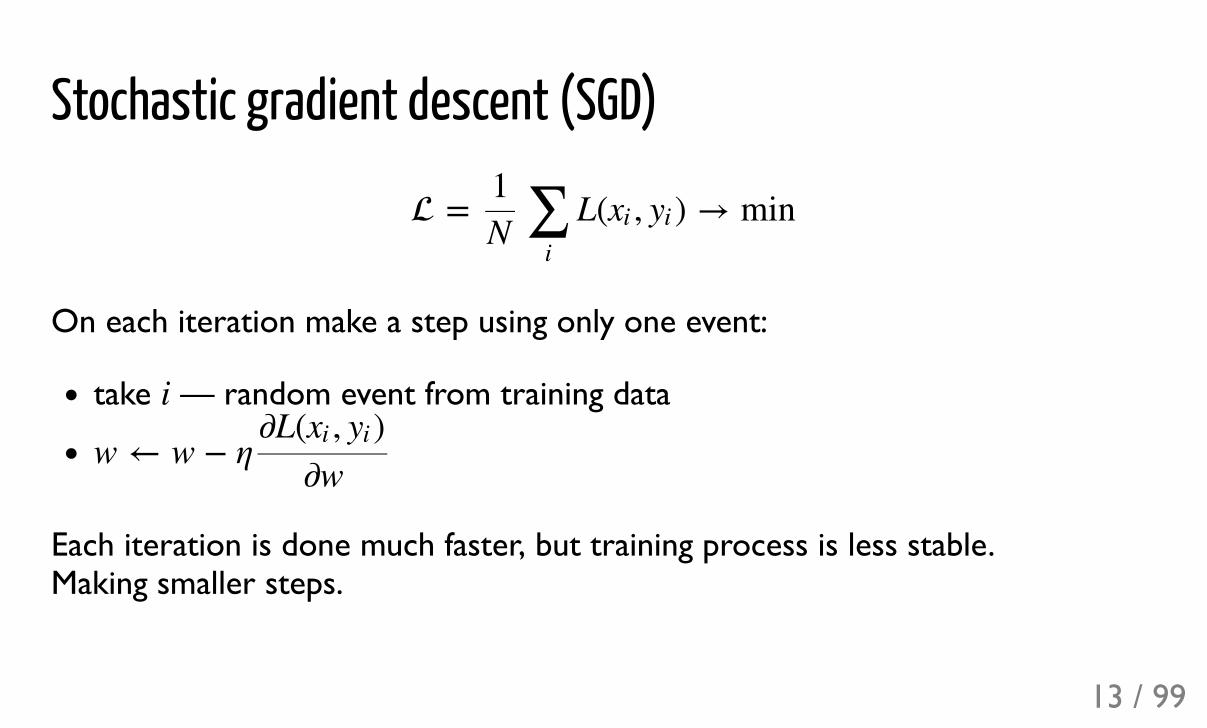
Stochastic gradient descent (SGD)
On each iteration make a step using only one event:
take — random event from training data
Each iteration is done much faster, but training process is less stable. Making smaller steps.
= L( , ) → min1N ∑
i
xi yi
i
w ← w + η�L( , )xi yi
�w
13 / 99
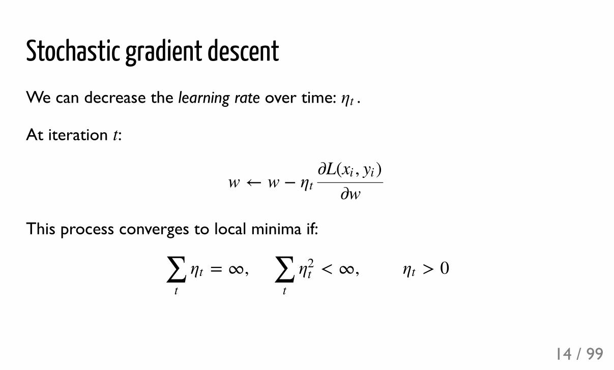
Stochastic gradient descentWe can decrease the learning rate over time: .
At iteration :
This process converges to local minima if:
ηt
t
w ← w + ηt�L( , )xi yi
�w
= 7, < 7, > 0∑t
ηt ∑t
η2t ηt
14 / 99
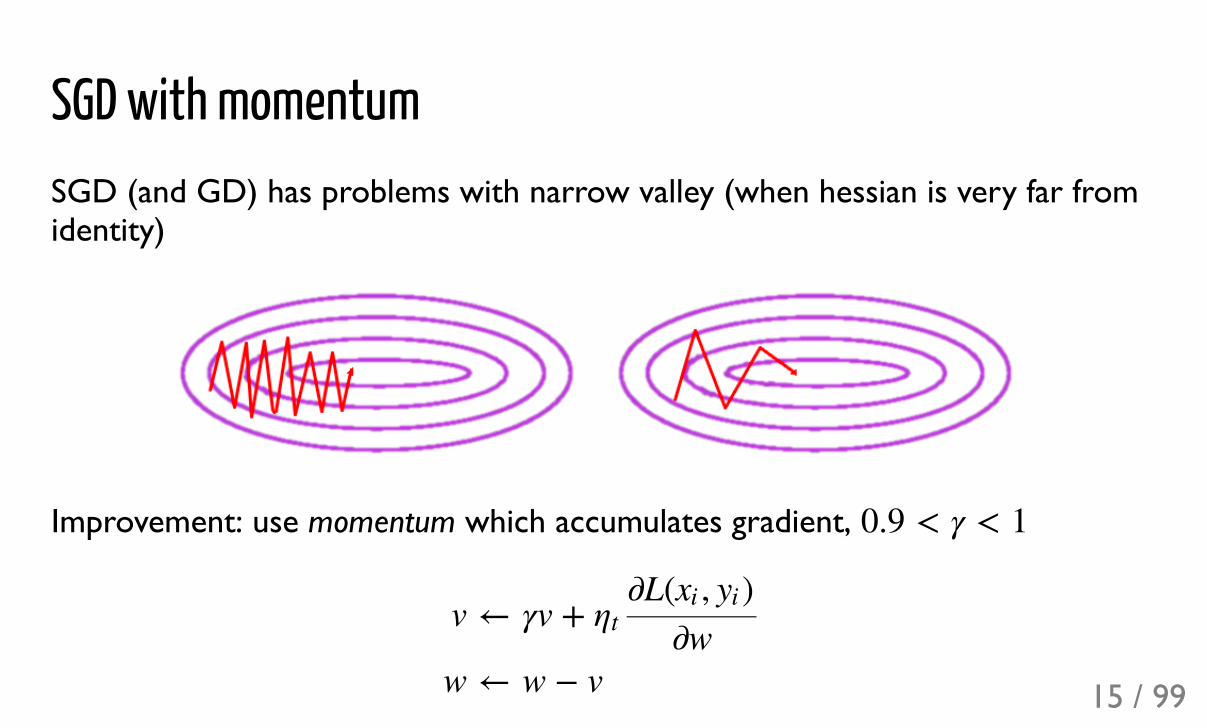
SGD with momentumSGD (and GD) has problems with narrow valley (when hessian is very far fromidentity)
Improvement: use momentum which accumulates gradient, 0.9 < γ < 1
v
w
←
←
γv + ηt�L( , )xi yi
�ww + v 15 / 99
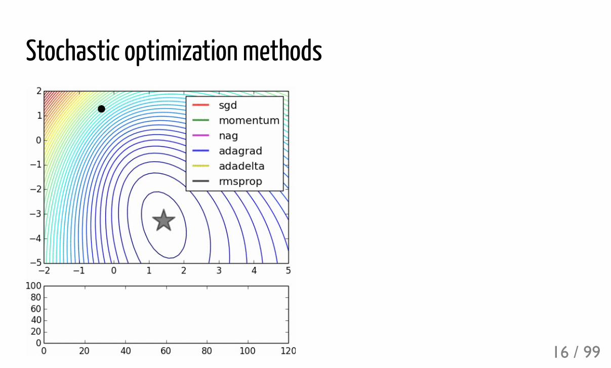
Stochastic optimization methods
16 / 99
Stochastic optimization methodsapplied to additive loss function
should be preferred when optimization time is the bottleneckmore advanced modifications exist:
AdaDelta, RMSProp, Adam.those are using adaptive step size (individually for each sample)crucial when scale of gradients is very different
in practice predictions are computed using minibatches (small groups of 16to 256 samples) not on event-by-event basis
= L( , )∑i
xi yi
17 / 99
Polynomial decision rule
d(x) = + +w0 ∑i
wi xi ∑ij
wijxixj
18 / 99
Polynomial decision rule
is again a linear model, introduce extended set of features:
and reuse logistic regression.
d(x) = + +w0 ∑i
wi xi ∑ij
wijxixj
z = {1} C { C {xi}i xixj}ij
d(x) = =< w, z >∑i
wi zi
19 / 99
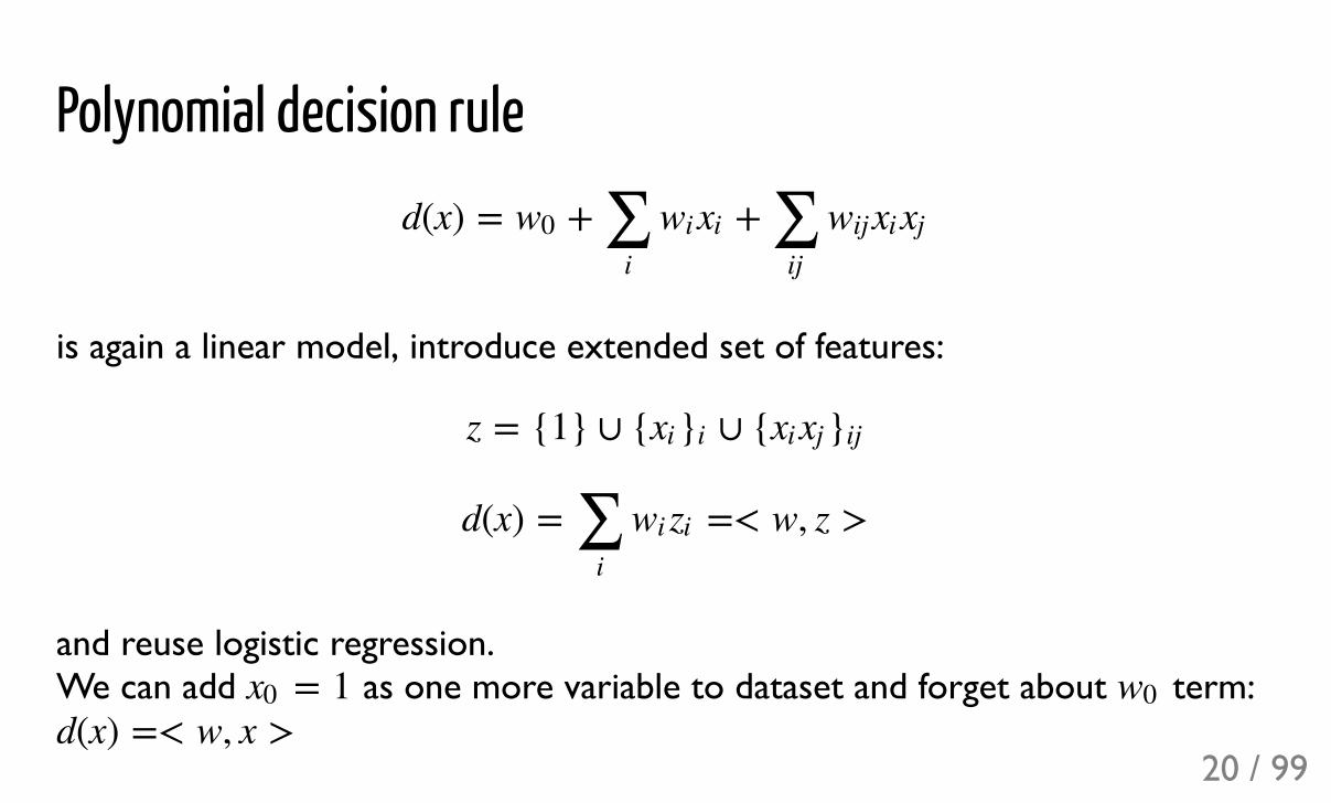
Polynomial decision rule
is again a linear model, introduce extended set of features:
and reuse logistic regression. We can add as one more variable to dataset and forget about term:
d(x) = + +w0 ∑i
wi xi ∑ij
wijxixj
z = {1} C { C {xi}i xixj}ij
d(x) = =< w, z >∑i
wi zi
= 1x0 w0d(x) =< w, x >
20 / 99
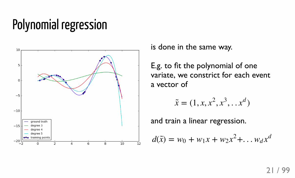
Polynomial regressionis done in the same way.
E.g. to fit the polynomial of onevariate, we constrict for each eventa vector of
and train a linear regression.
= (1, x, , , . . )x x2 x3 xd
d( ) = + x + +. . .x w0 w1 w2x2 wd xd
21 / 99
Projecting into the space of higher dimension
SVM with polynomial kernel visualization
22 / 99
Logistic regression overviewclassifier based on linear decision ruletraining is reduced to convex optimizationstochastic optimization can be usedcan handle > 1000 features, but requires regularization (see later)no interaction between features
other decision rules are achieved by adding new features
23 / 99
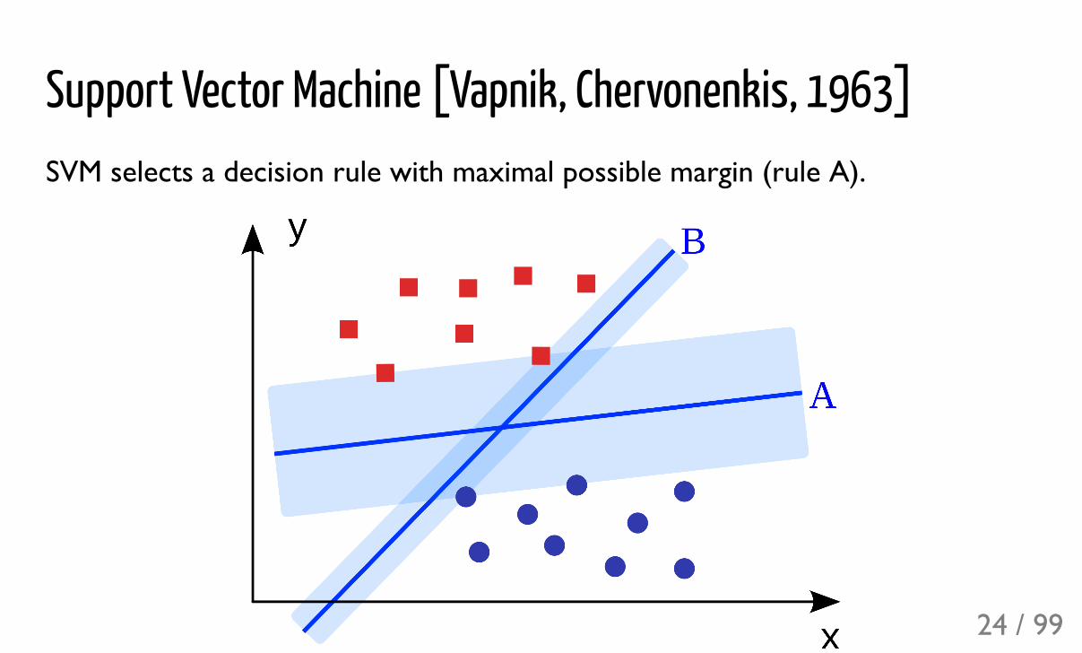
Support Vector Machine [Vapnik, Chervonenkis, 1963]SVM selects a decision rule with maximal possible margin (rule A).
24 / 99
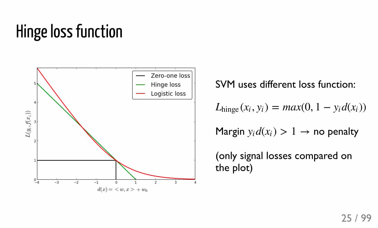
Hinge loss function
SVM uses different loss function:
Margin no penalty
(only signal losses compared onthe plot)
( , ) = max(0, 1 + d( ))Lhinge xi yi yi xi
d( ) > 1 →yi xi
25 / 99
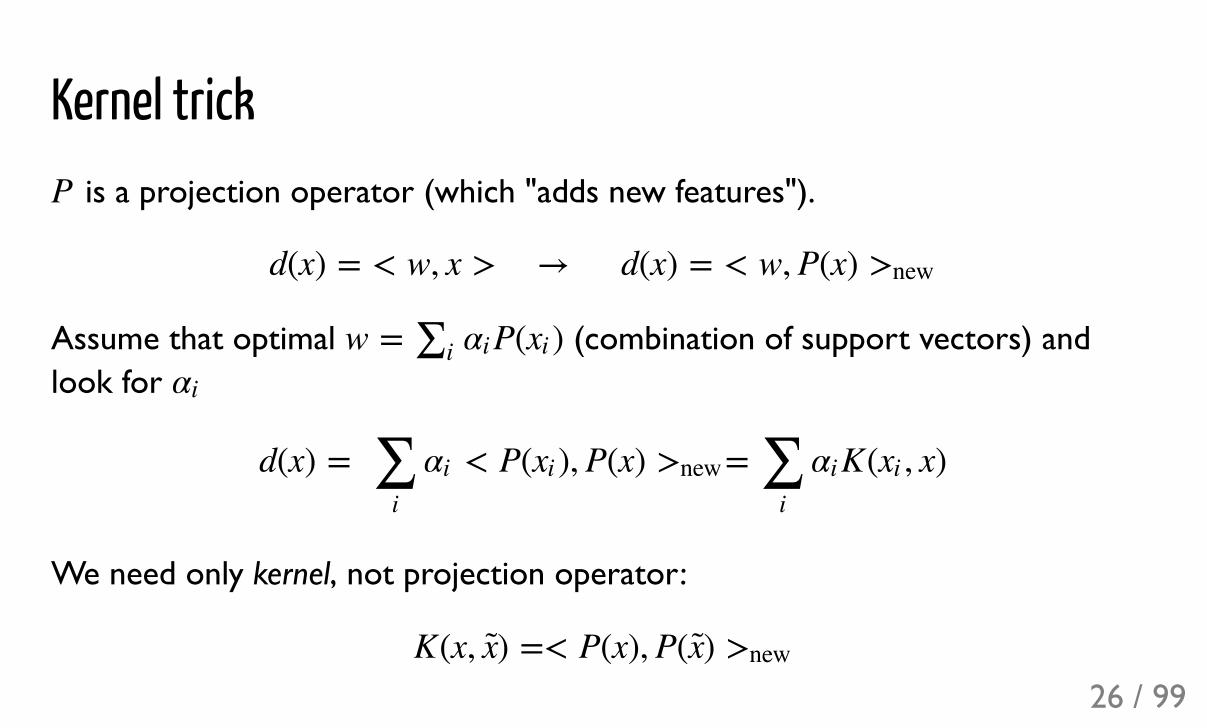
Kernel trick is a projection operator (which "adds new features").
Assume that optimal (combination of support vectors) andlook for
We need only kernel, not projection operator:
P
d(x) = < w, x > → d(x) = < w, P(x) >new
w = P( )*i αi xi
αi
d(x) = < P( ), P(x) = K( , x)∑i
αi xi >new ∑i
αi xi
K(x, ) =< P(x), P( )x x >new
26 / 99
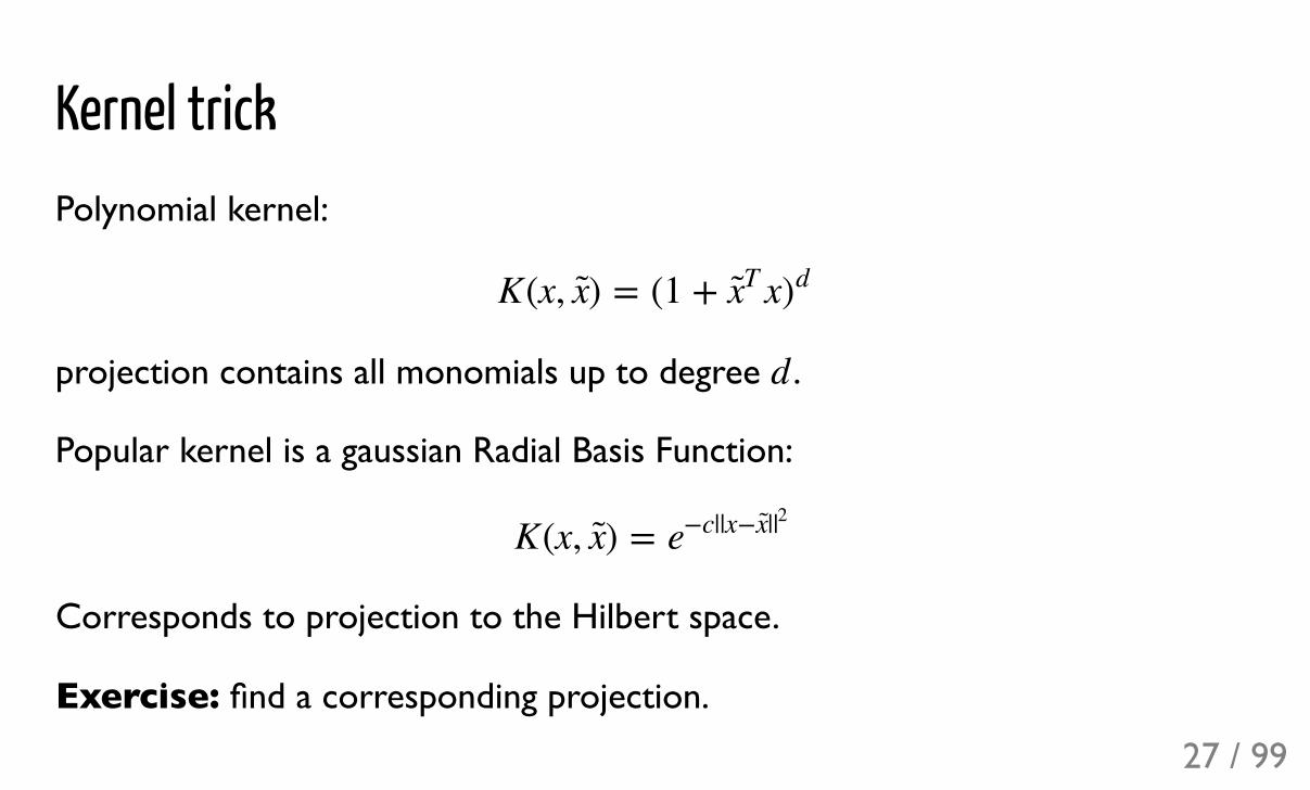
Kernel trickPolynomial kernel:
projection contains all monomials up to degree .
Popular kernel is a gaussian Radial Basis Function:
Corresponds to projection to the Hilbert space.
Exercise: find a corresponding projection.
K(x, ) = (1 + xx x T )d
d
K(x, ) =x e+c||x+ |x |2
27 / 99
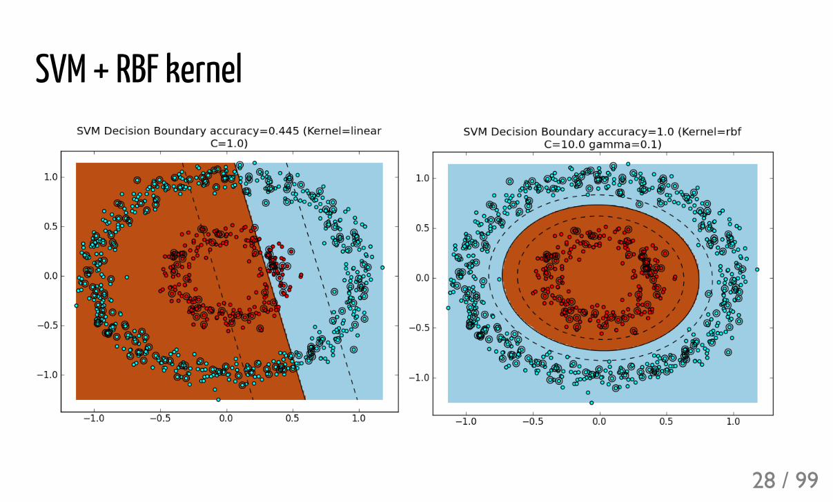
SVM + RBF kernel
28 / 99
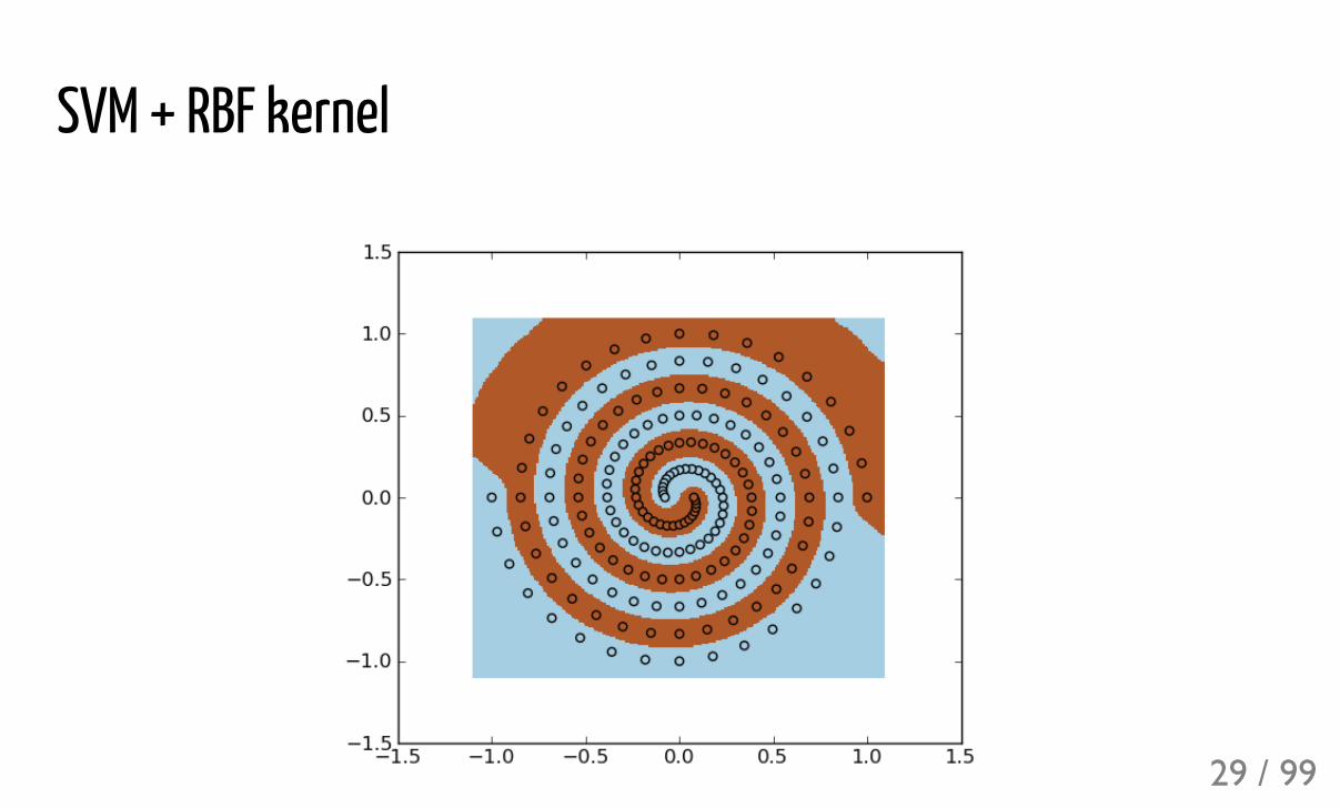
SVM + RBF kernel
29 / 99
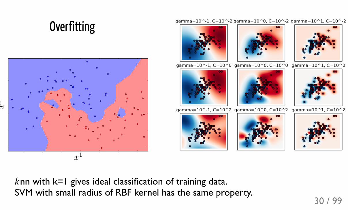
Overfitting
nn with k=1 gives ideal classification of training data. SVM with small radius of RBF kernel has the same property.k
30 / 99
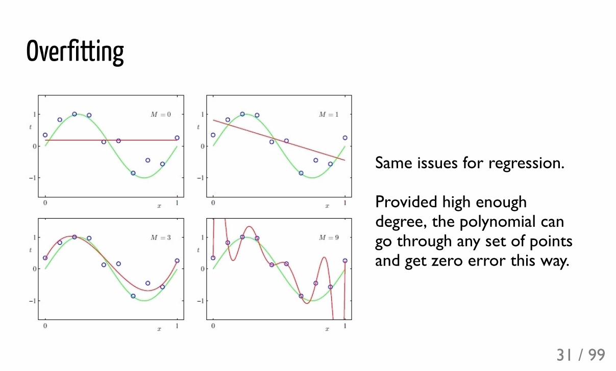
Overfitting
Same issues for regression.
Provided high enoughdegree, the polynomial cango through any set of pointsand get zero error this way.
31 / 99
There are two definitions of overfitting, which often coincide.
Difference-overfitting
(academical definition)
There is a significant difference in quality of predictions between train andholdout.
Complexity-overfitting
(practitioners' definition)
Formula has too high complexity (e.g. too many parameters), increasing thenumber of parameters drives to lower quality.
32 / 99

Model selectionGiven two models, which one should we select?
33 / 99
Model selectionGiven two models, which one should we select?
ML is about inference of statistical dependencies, which give us ability to predict
The best model is the model which gives better predictions for newobservations.
Simplest way to control this is to check quality on a holdout — a sample notused during training (cross-validation). This gives unbiased estimate of quality fornew data.
estimates have variancemultiple testing introduces bias (solution: train + validation + test, likekaggle)
34 / 99
Difference-overfitting is inessential, provided that we measure quality on aholdout sample (though easy to check and sometimes helpful).
Complexity-overfitting is a problem — we need to test different parameters foroptimality (more examples through the course).
35 / 99
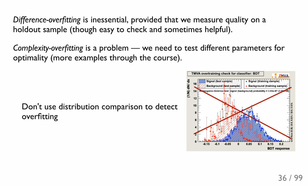
Difference-overfitting is inessential, provided that we measure quality on aholdout sample (though easy to check and sometimes helpful).
Complexity-overfitting is a problem — we need to test different parameters foroptimality (more examples through the course).
Don't use distribution comparison to detectoverfitting
36 / 99
-minutes breakn2
37 / 99
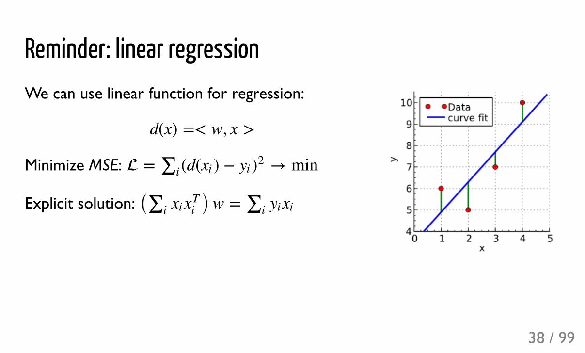
Reminder: linear regressionWe can use linear function for regression:
Minimize MSE:
Explicit solution:
d(x) =< w, x >
= (d( ) + → min*i xi yi )2
( ) w =*i xixTi *i yixi
38 / 99
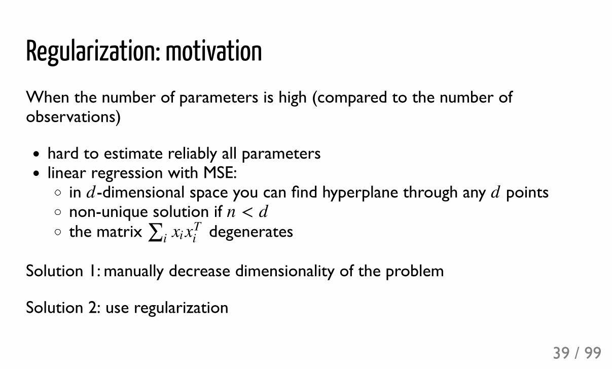
Regularization: motivationWhen the number of parameters is high (compared to the number ofobservations)
hard to estimate reliably all parameterslinear regression with MSE:
in -dimensional space you can find hyperplane through any pointsnon-unique solution if the matrix degenerates
Solution 1: manually decrease dimensionality of the problem
Solution 2: use regularization
d dn < d
*i xixTi
39 / 99
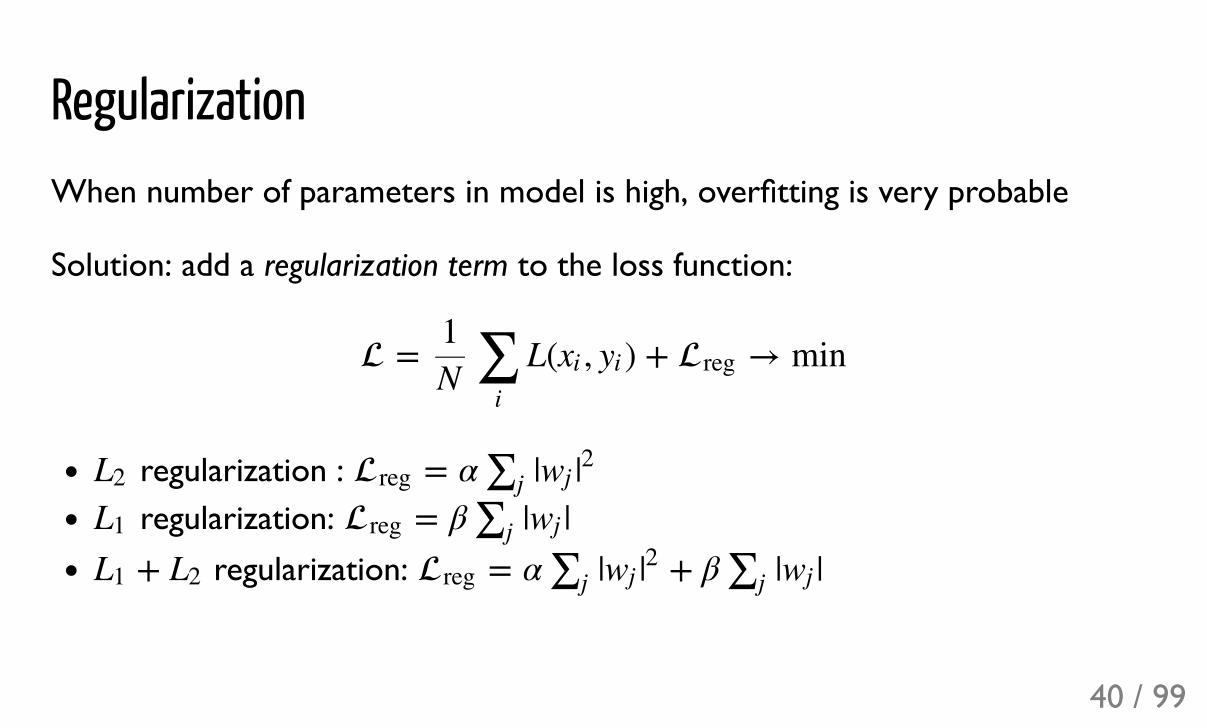
RegularizationWhen number of parameters in model is high, overfitting is very probable
Solution: add a regularization term to the loss function:
regularization : regularization:
regularization:
= L( , ) + → min1N ∑
i
xi yi reg
L2 = α |reg *j wj |2
L1 = β | |reg *j wj
+L1 L2 = α | + β | |reg *j wj |2 *j wj
40 / 99
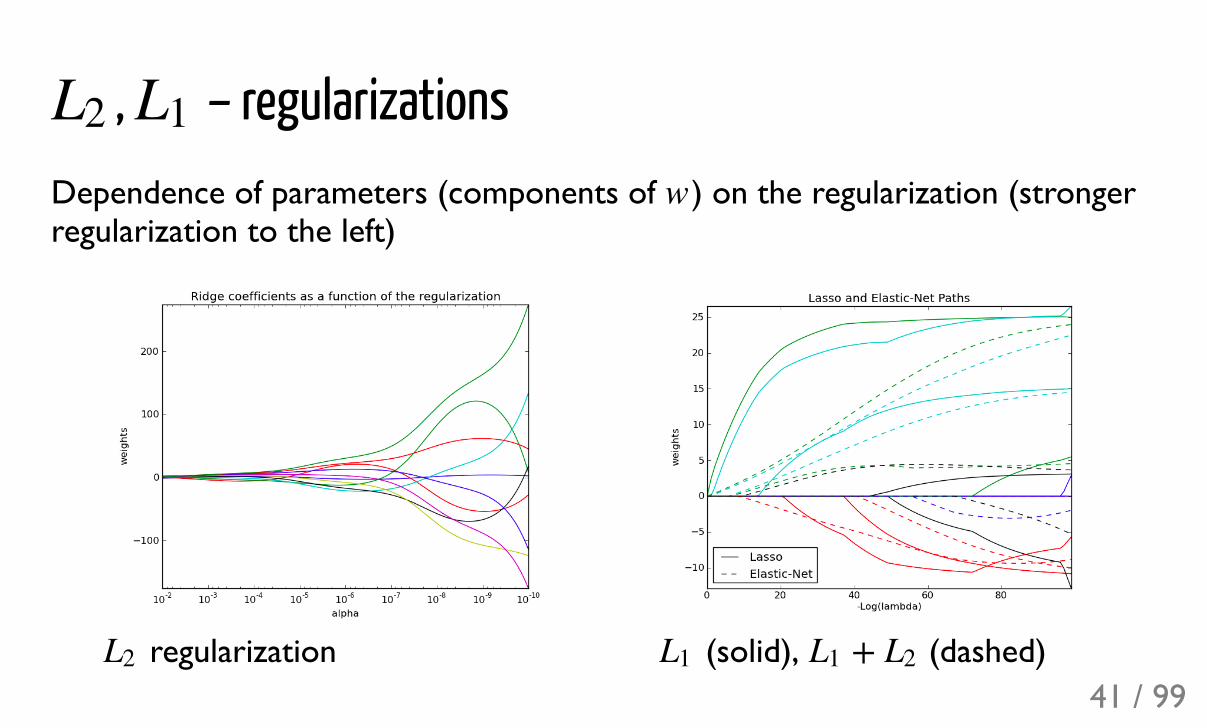
, – regularizationsDependence of parameters (components of ) on the regularization (strongerregularization to the left)
regularization
(solid), (dashed)
L2 L1
w
L2 L1 +L1 L2
41 / 99
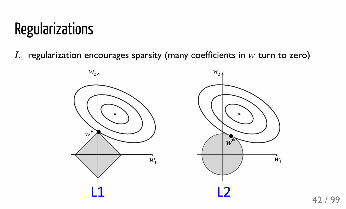
Regularizations regularization encourages sparsity (many coefficients in turn to zero)L1 w
42 / 99
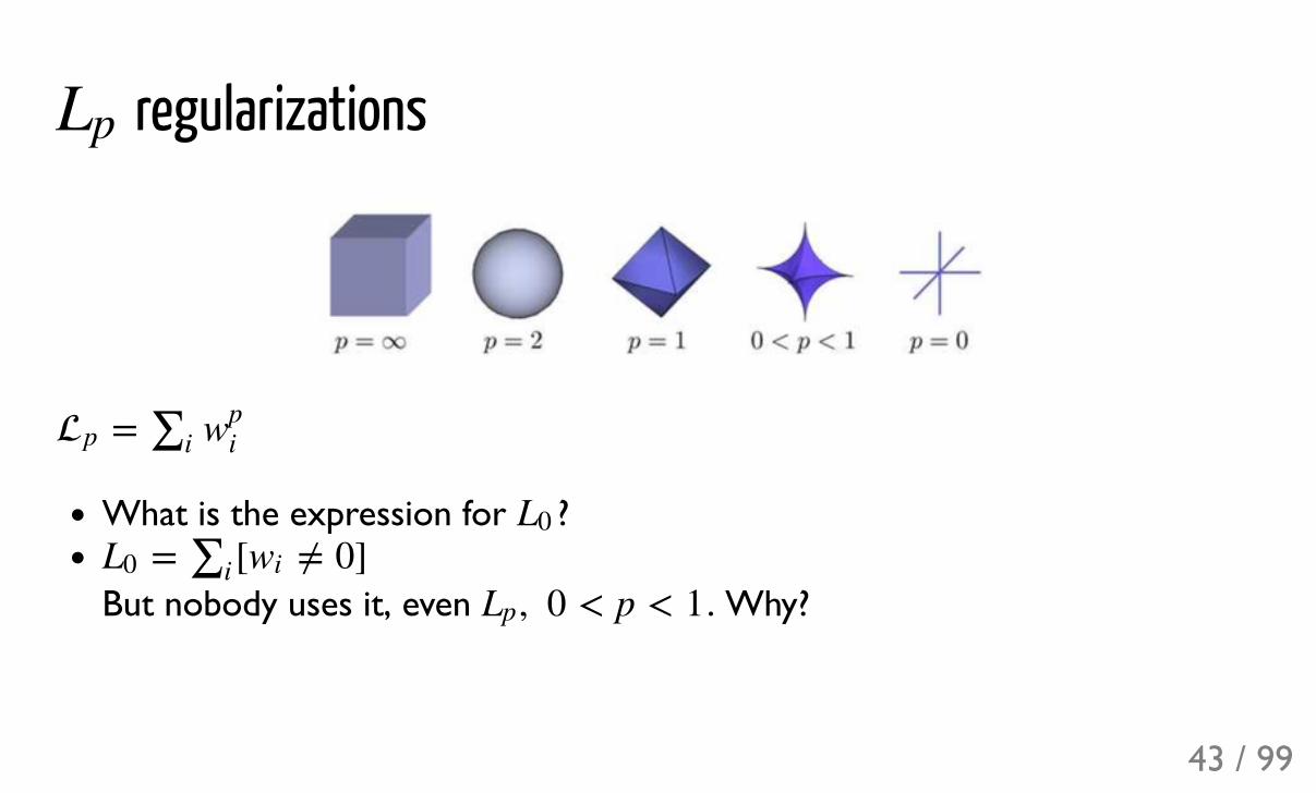
regularizations
What is the expression for ?
But nobody uses it, even . Why?
Lp
=p *i wpi
L0= [ y 0]L0 *i wi
, 0 < p < 1Lp
43 / 99
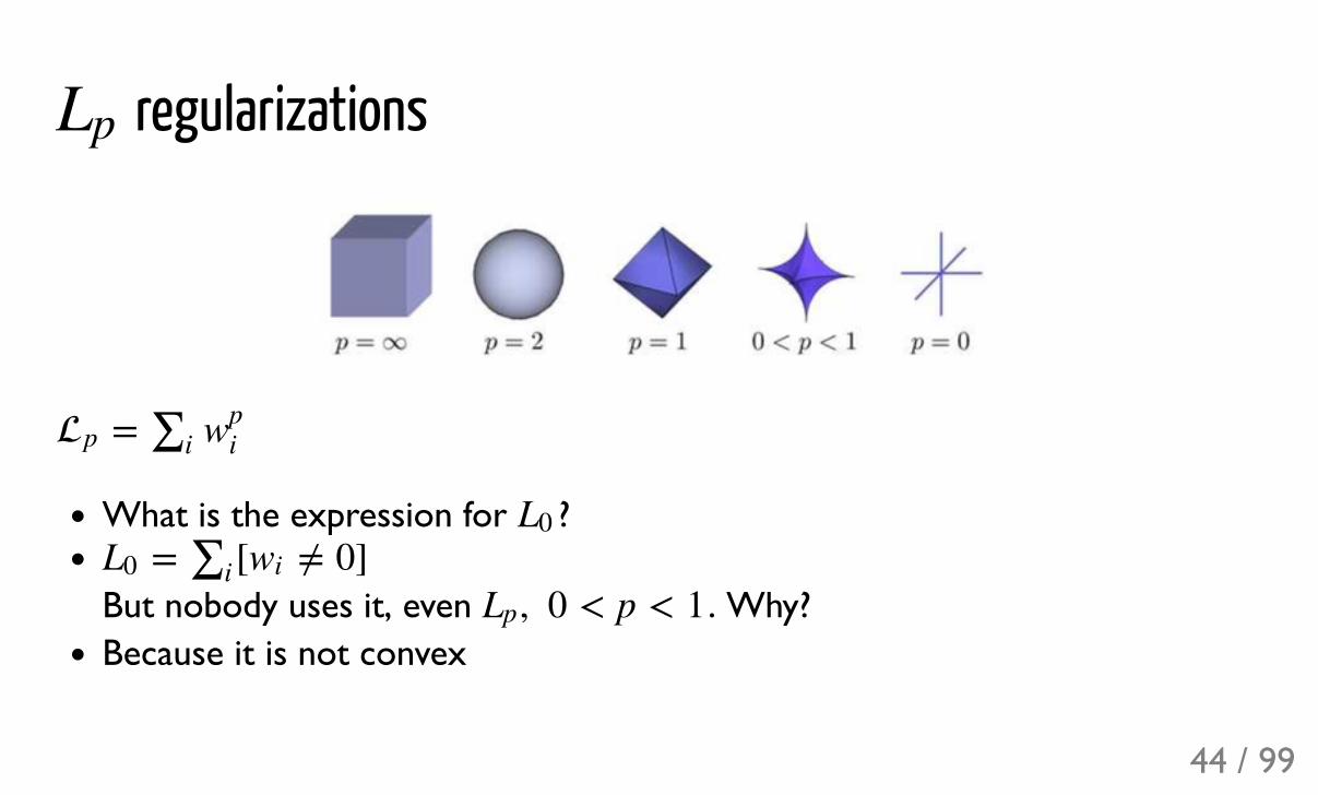
regularizations
What is the expression for ?
But nobody uses it, even . Why?Because it is not convex
Lp
=p *i wpi
L0= [ y 0]L0 *i wi
, 0 < p < 1Lp
44 / 99
Regularization summaryimportant tool to fight overfitting (= poor generalization on a new data)different modifications for other modelsmakes it possible to handle really many featuresmachine learning should detect important features itselffrom mathematical point: turning convex problem to strongly convex (NB: only for linear models)from practical point: softly limiting the space of parametersbreaks scale-invariance of linear models
45 / 99
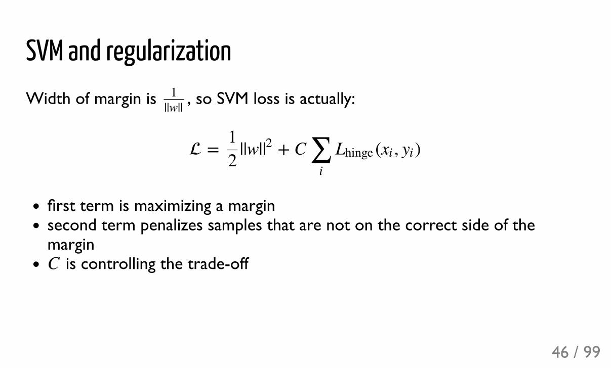
SVM and regularization
Width of margin is , so SVM loss is actually:
first term is maximizing a marginsecond term penalizes samples that are not on the correct side of themargin
is controlling the trade-off
1||w||
= ||w| + C ( , )12
|2 ∑i
Lhinge xi yi
C
46 / 99
Linear models summarylinear decision function in the corereduced to optimization problemslosses are additive
stochastic optimizations applicablecan support nonlinear decisions w.r.t. to original features by using kernelsapply regularizations to avoid bad situations and overfitting
= L( , )∑i
xi yi
47 / 99
Decision Trees
48 / 99
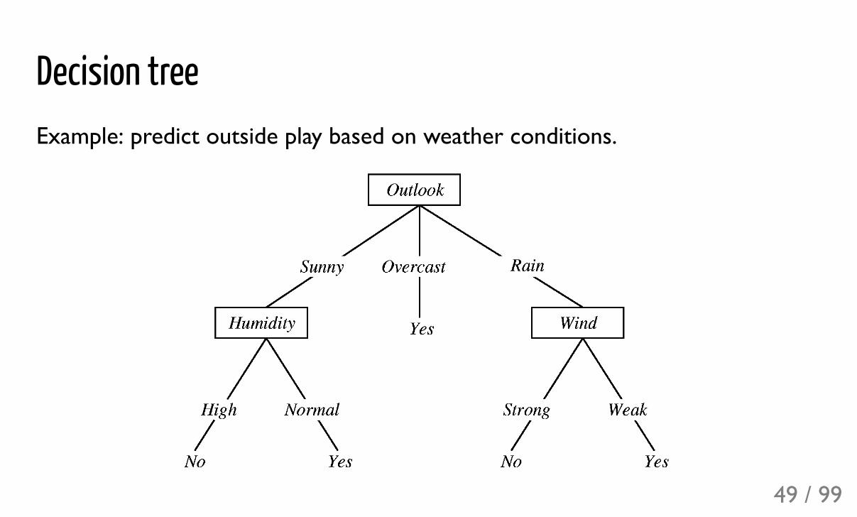
Decision treeExample: predict outside play based on weather conditions.
49 / 99
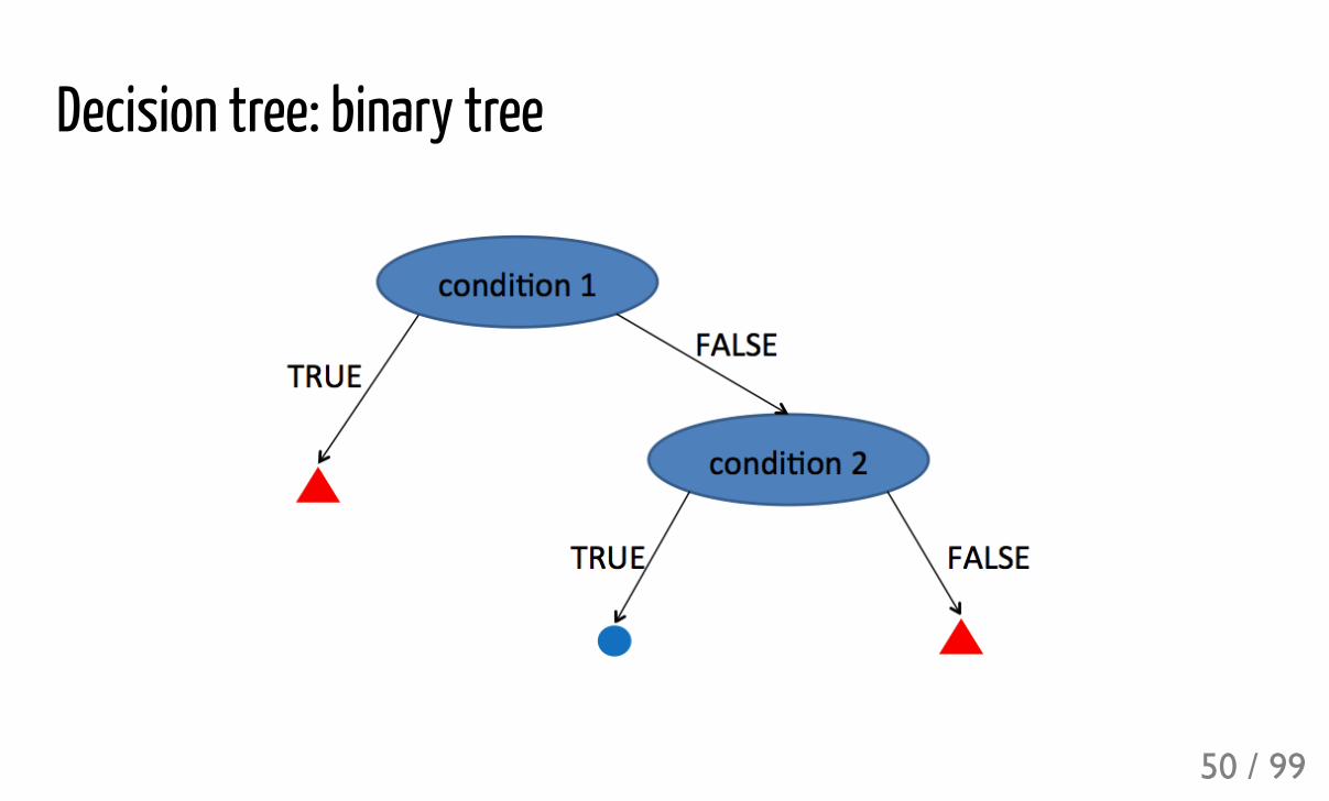
Decision tree: binary tree
50 / 99
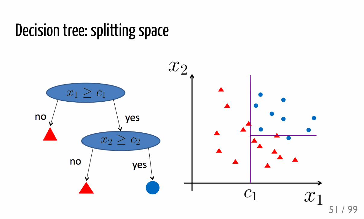
Decision tree: splitting space
51 / 99
Decision treefast & intuitive predictionbut building an optimal decision tree is an NP complete problem
52 / 99
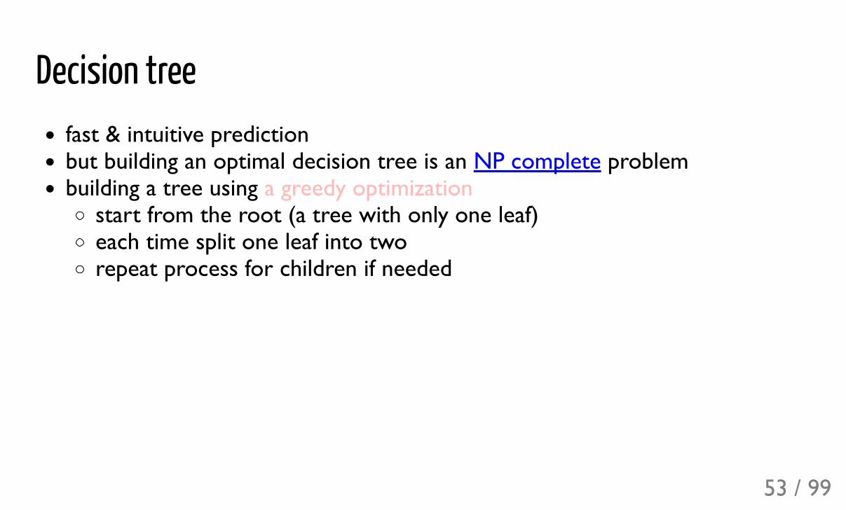
Decision treefast & intuitive predictionbut building an optimal decision tree is an NP complete problembuilding a tree using a greedy optimization
start from the root (a tree with only one leaf)each time split one leaf into tworepeat process for children if needed
53 / 99
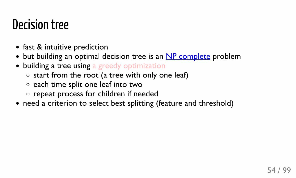
Decision treefast & intuitive predictionbut building an optimal decision tree is an NP complete problembuilding a tree using a greedy optimization
start from the root (a tree with only one leaf)each time split one leaf into tworepeat process for children if needed
need a criterion to select best splitting (feature and threshold)
54 / 99
Splitting criterion
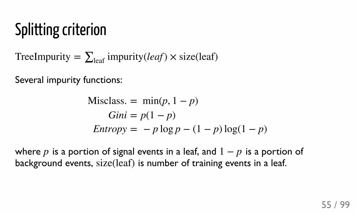
Several impurity functions:
where is a portion of signal events in a leaf, and is a portion ofbackground events, is number of training events in a leaf.
TreeImpurity = impurity(leaf ) × size(leaf)*leaf
Misclass.Gini
Entropy
===
min(p, 1 + p)p(1 + p)+ p log p + (1 + p) log(1 + p)
p 1 + psize(leaf)
55 / 99
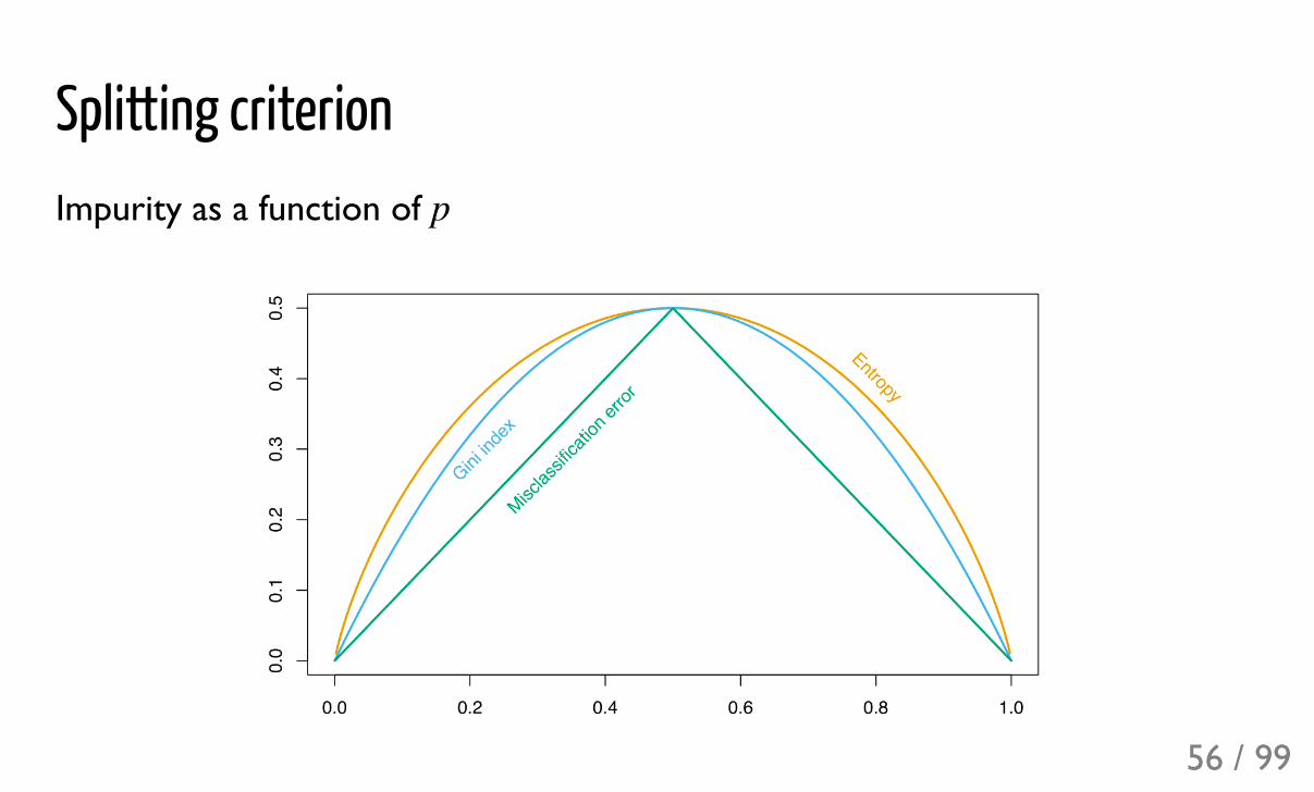
Splitting criterionImpurity as a function of p
56 / 99
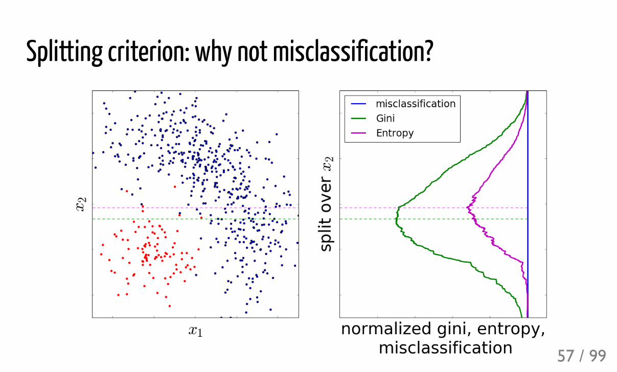
Splitting criterion: why not misclassification?
57 / 99
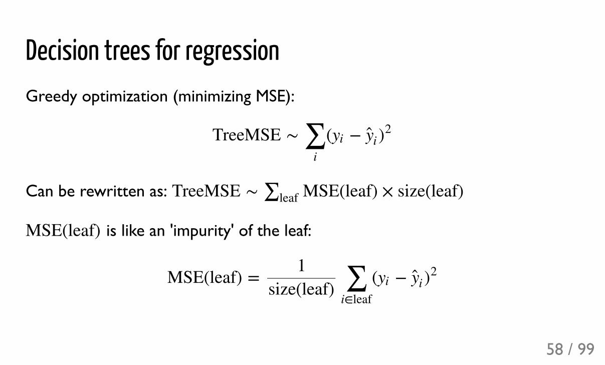
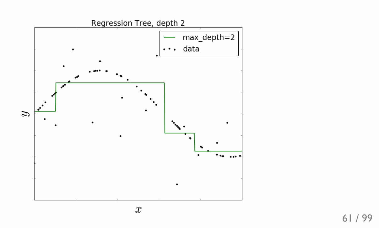
Decision trees for regressionGreedy optimization (minimizing MSE):
Can be rewritten as:
is like an 'impurity' of the leaf:
TreeMSE U ( +∑i
yi y i )2
TreeMSE U MSE(leaf) × size(leaf)*leaf
MSE(leaf)
MSE(leaf) = ( +1
size(leaf) ∑i!leaf
yi y i )2
58 / 99
59 / 99
60 / 99
61 / 99
62 / 99
63 / 99
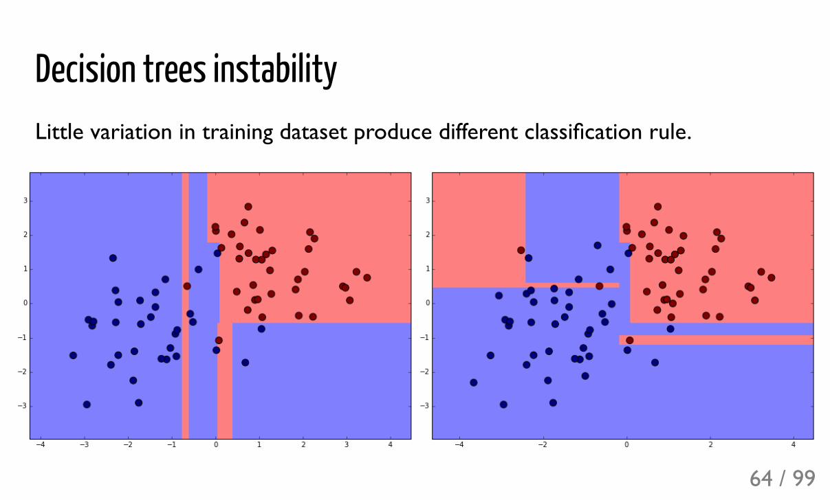
Decision trees instabilityLittle variation in training dataset produce different classification rule.
64 / 99
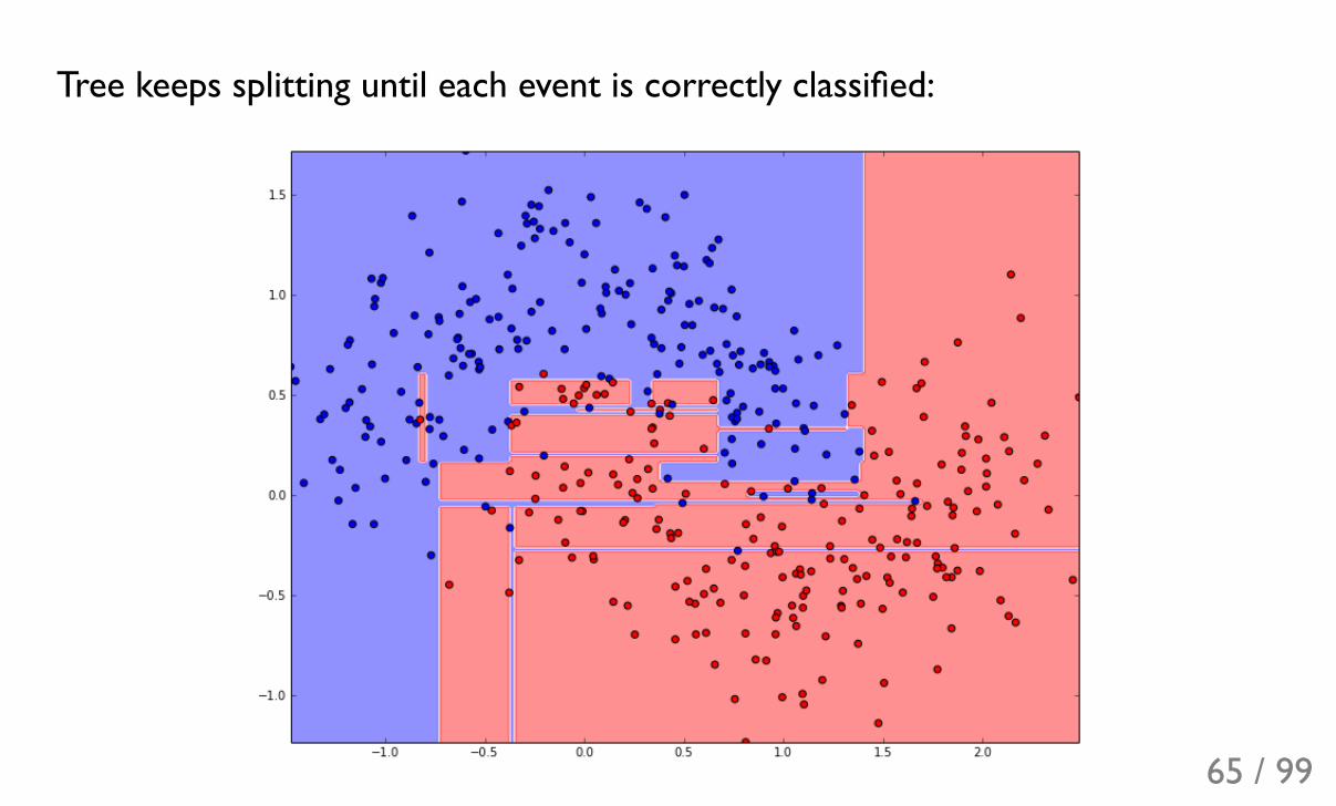
Tree keeps splitting until each event is correctly classified:
65 / 99
Pre-stoppingWe can stop the process of splitting by imposing different restrictions:
limit the depth of treeset minimal number of samples needed to split the leaflimit the minimal number of samples in leafmore advanced: maximal number of leaves in tree
66 / 99
Pre-stoppingWe can stop the process of splitting by imposing different restrictions:
limit the depth of treeset minimal number of samples needed to split the leaflimit the minimal number of samples in leafmore advanced: maximal number of leaves in tree
Any combinations of rules above is possible.
67 / 99
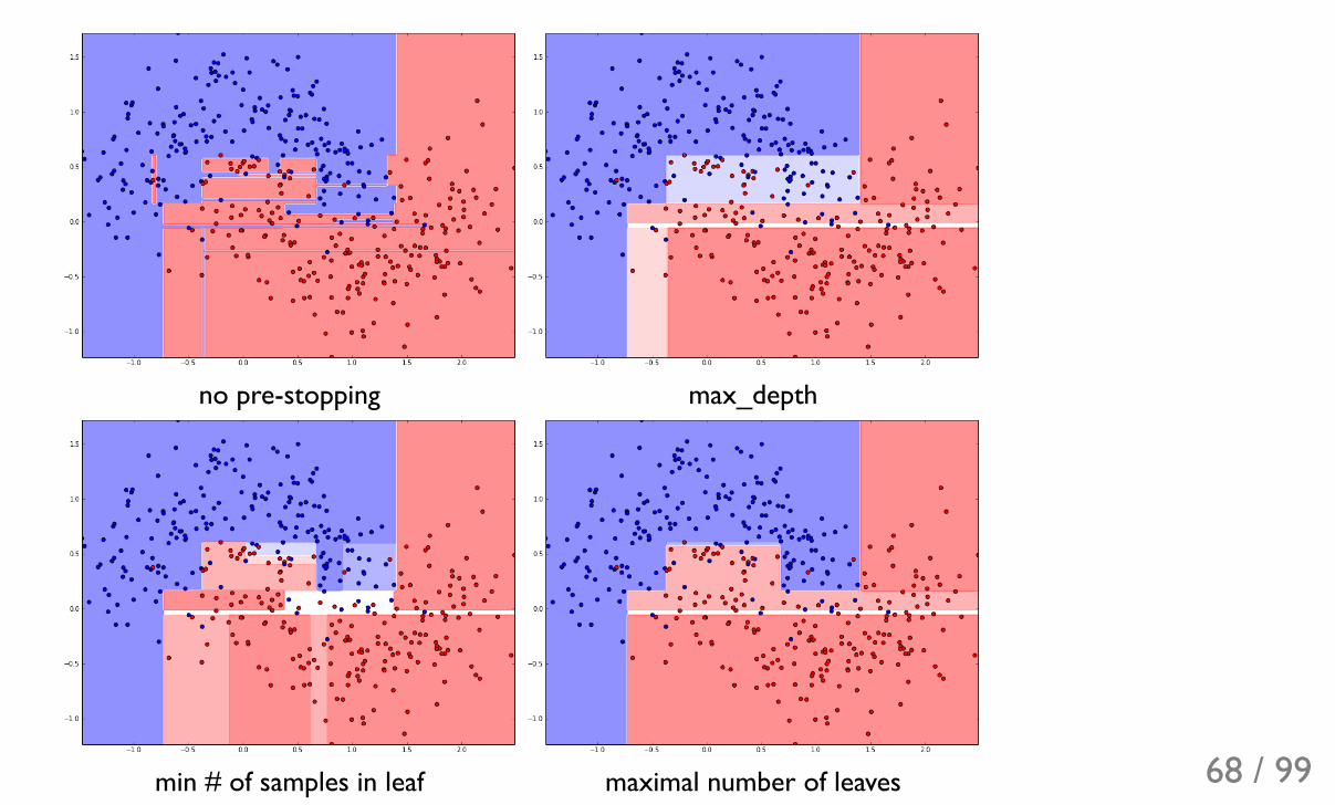
no pre-stopping max_depth
min # of samples in leaf maximal number of leaves 68 / 99
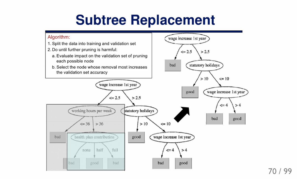
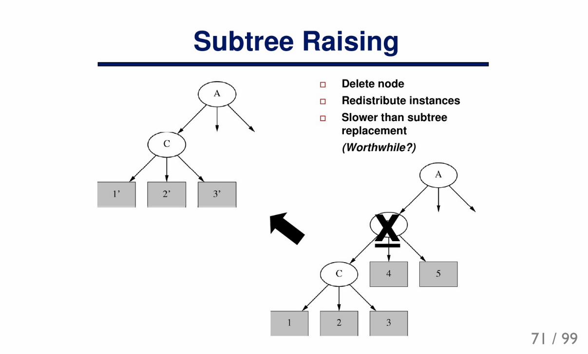
Post-pruningWhen a tree is already built we can try optimize it to simplify formula.
Generally, much slower than pre-stopping.
69 / 99
70 / 99
71 / 99
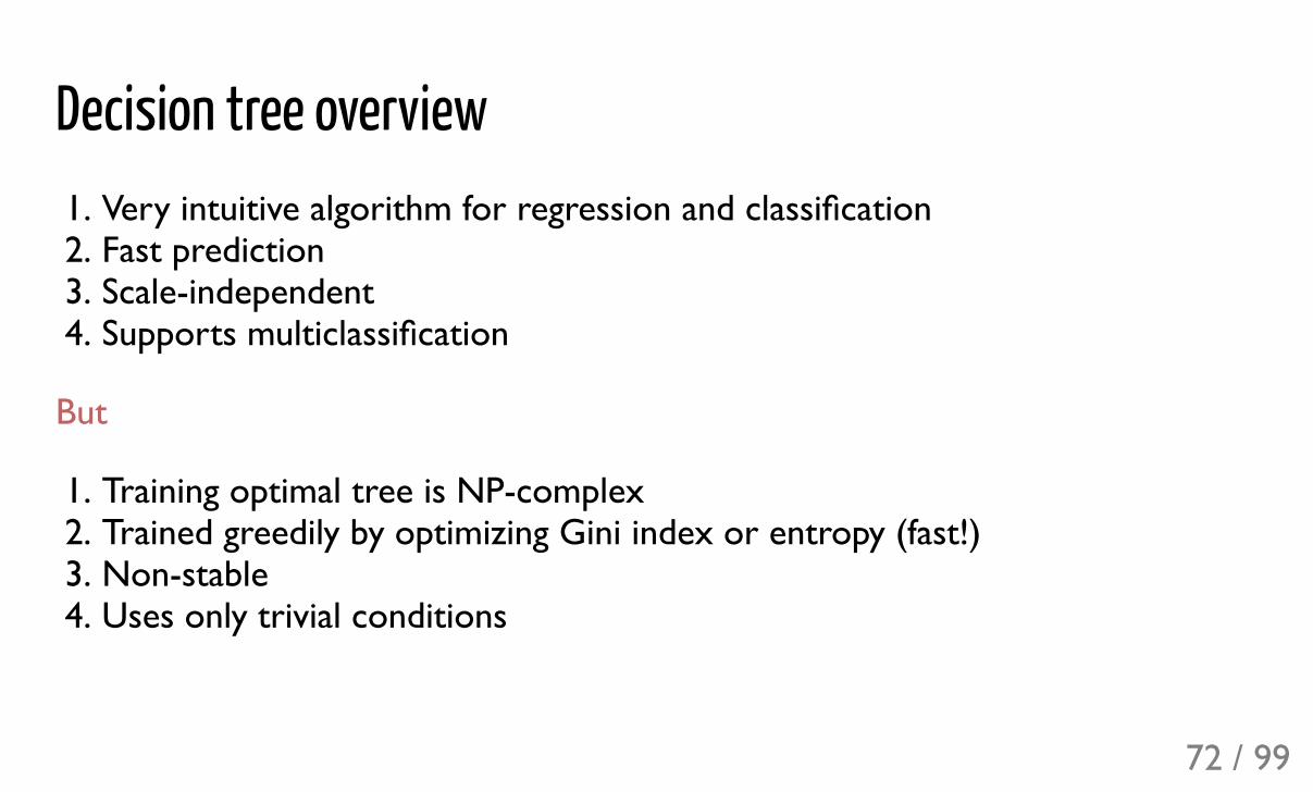
Decision tree overview1. Very intuitive algorithm for regression and classification2. Fast prediction3. Scale-independent4. Supports multiclassification
But
1. Training optimal tree is NP-complex2. Trained greedily by optimizing Gini index or entropy (fast!)3. Non-stable4. Uses only trivial conditions
72 / 99
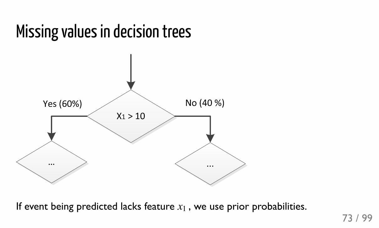
Missing values in decision trees
If event being predicted lacks feature , we use prior probabilities.x173 / 99
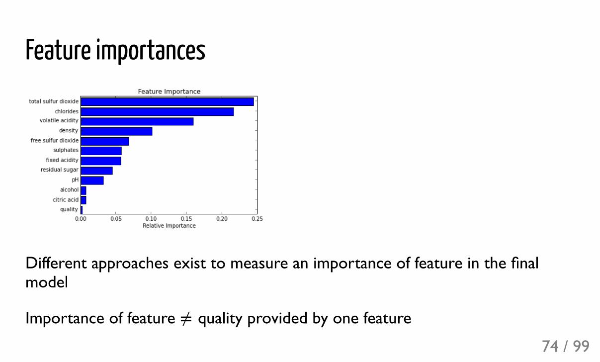
Feature importances
Different approaches exist to measure an importance of feature in the finalmodel
Importance of feature quality provided by one featurey74 / 99
Feature importancestree: counting number of splits made over this feature
75 / 99
Feature importancestree: counting number of splits made over this featuretree: counting gain in purity (e.g. Gini) fast and adequate
76 / 99
Feature importancestree: counting number of splits made over this featuretree: counting gain in purity (e.g. Gini) fast and adequatemodel-agnostic recipe: train without one feature, compare quality on test with/without one feature
requires many evaluations
77 / 99
Feature importancestree: counting number of splits made over this featuretree: counting gain in purity (e.g. Gini) fast and adequatemodel-agnostic recipe: train without one feature, compare quality on test with/without one feature
requires many evaluations
model-agnostic recipe: feature shuffling
take one column in test dataset and shuffle it. Compare quality with/withoutshuffling.
78 / 99
Ensembles
79 / 99
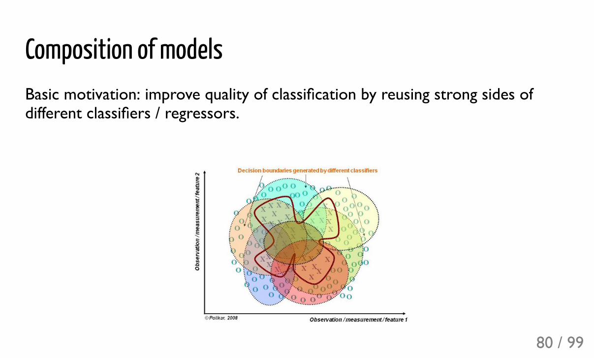
Composition of modelsBasic motivation: improve quality of classification by reusing strong sides ofdifferent classifiers / regressors.
80 / 99
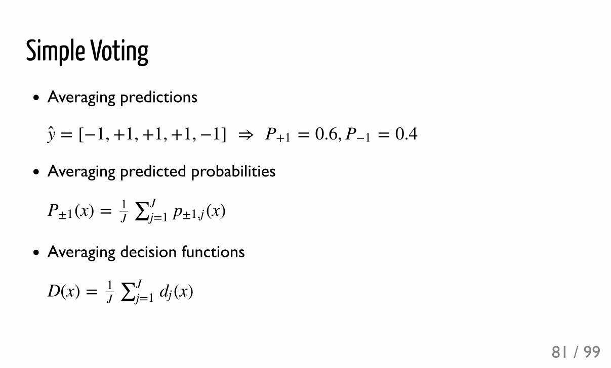
Simple VotingAveraging predictions
Averaging predicted probabilities
Averaging decision functions
= [+1, +1, +1, +1,+1] ⇒ = 0.6, = 0.4y P+1 P+1
(x) = (x)P±11J *
Jj=1 p±1,j
D(x) = (x)1J *
Jj=1 dj
81 / 99
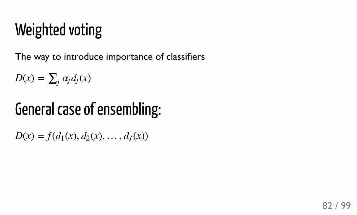
Weighted votingThe way to introduce importance of classifiers
General case of ensembling:
D(x) = (x)*j αjdj
D(x) = f ( (x), (x),… , (x))d1 d2 dJ
82 / 99
Problems
very close base classifiersneed to keep variationand still have good quality of basic classifiers
83 / 99
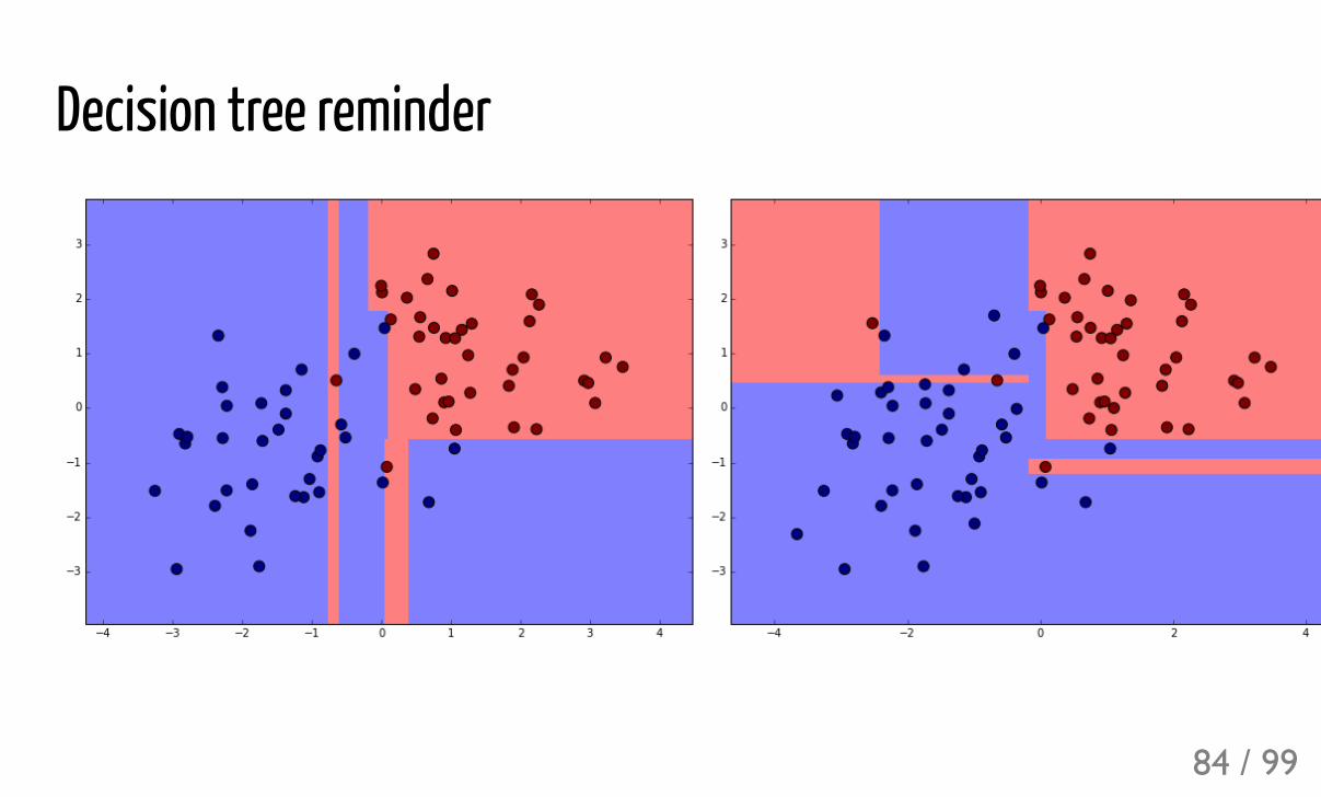
Decision tree reminder
84 / 99
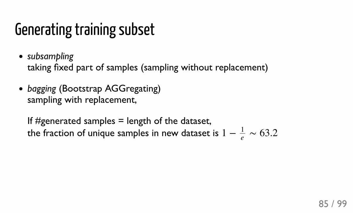
Generating training subsetsubsampling taking fixed part of samples (sampling without replacement)
bagging (Bootstrap AGGregating) sampling with replacement,
If #generated samples = length of the dataset, the fraction of unique samples in new dataset is 1 + U 63.21
e
85 / 99
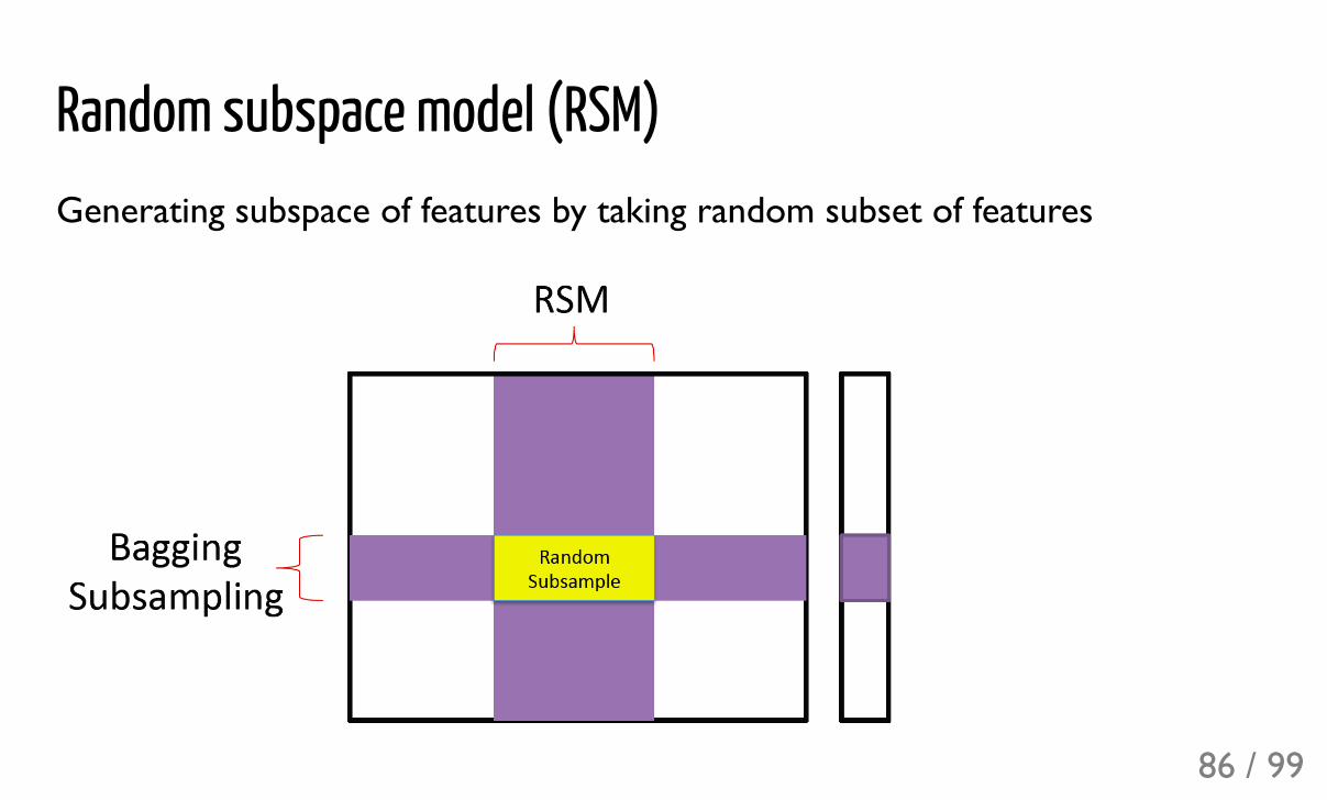
Random subspace model (RSM)Generating subspace of features by taking random subset of features
86 / 99
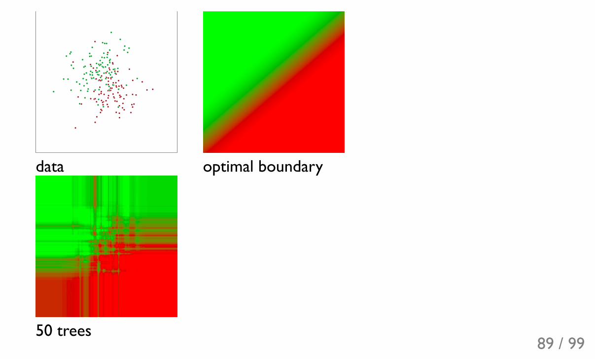
Random Forest [Leo Breiman, 2001]Random forest is a composition of decision trees.
Each individual tree is trained on a subset of training data obtained by
bagging samplestaking random subset of features
Predictions of random forest are obtained via simple voting.
87 / 99
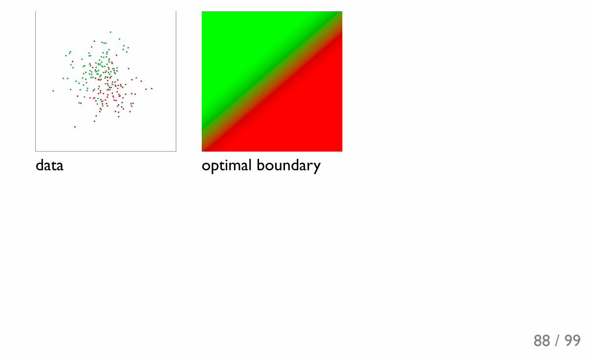
data optimal boundary
88 / 99
data optimal boundary
50 trees89 / 99
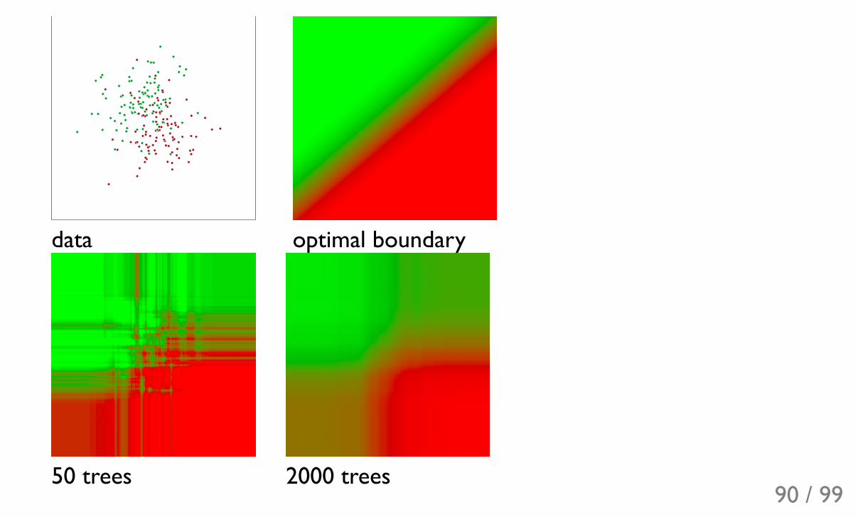
data optimal boundary
50 trees 2000 trees90 / 99

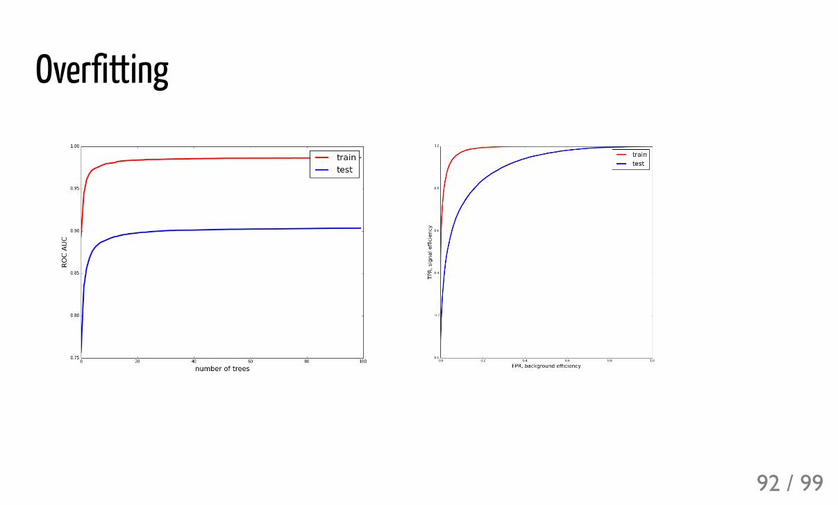
Overfitting
91 / 99
Overfitting
92 / 99
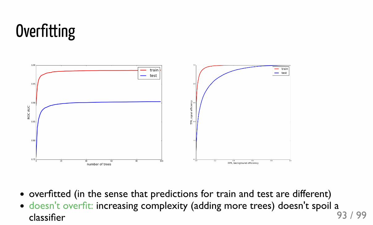
Overfitting
overfitted (in the sense that predictions for train and test are different)doesn't overfit: increasing complexity (adding more trees) doesn't spoil aclassifier 93 / 99

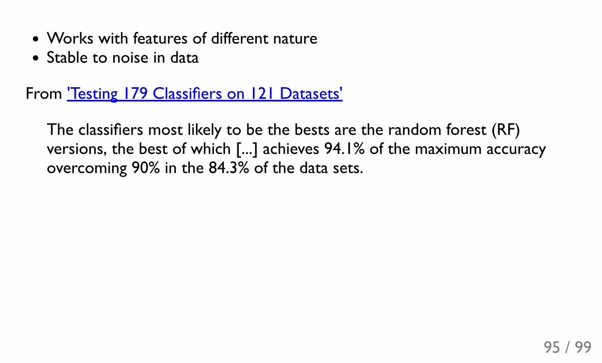
Works with features of different natureStable to noise in data
94 / 99
Works with features of different natureStable to noise in data
From 'Testing 179 Classifiers on 121 Datasets'
The classifiers most likely to be the bests are the random forest (RF)versions, the best of which [...] achieves 94.1% of the maximum accuracyovercoming 90% in the 84.3% of the data sets.
95 / 99
Random Forest overviewImpressively simpleTrees can be trained in parallelDoesn't overfit
96 / 99
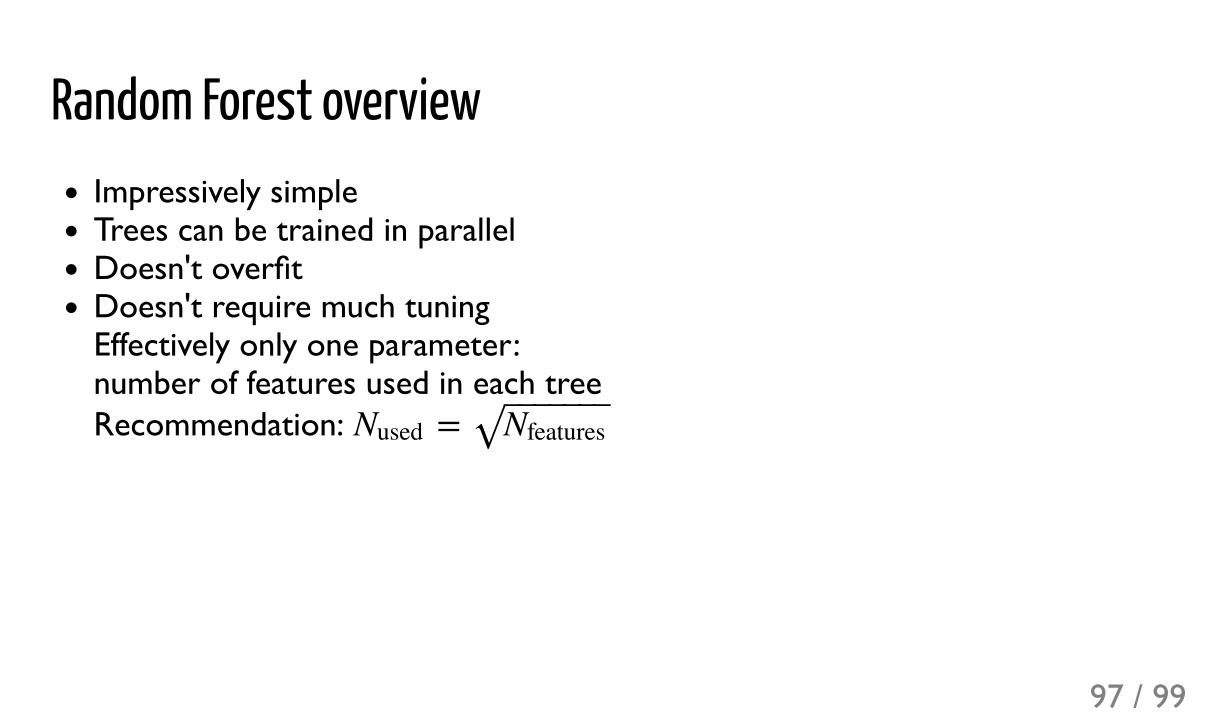
Random Forest overviewImpressively simpleTrees can be trained in parallelDoesn't overfitDoesn't require much tuning Effectively only one parameter: number of features used in each tree Recommendation: =Nused Nfeatures‾ ‾‾‾‾‾‾3
97 / 99
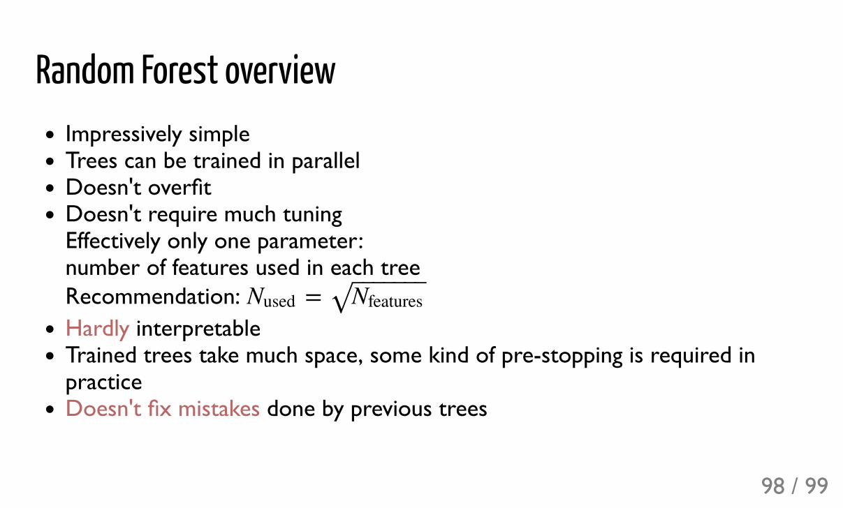
Random Forest overviewImpressively simpleTrees can be trained in parallelDoesn't overfitDoesn't require much tuning Effectively only one parameter: number of features used in each tree Recommendation: Hardly interpretableTrained trees take much space, some kind of pre-stopping is required inpracticeDoesn't fix mistakes done by previous trees
=Nused Nfeatures‾ ‾‾‾‾‾‾3
98 / 99

99 / 99