Embed Size (px)
Citation preview

Mathématiques - Informatique
Optimal Transport
From a Computer Perspective
Summer School « Geometric Measure Theory and
Calculus of Variations », Grenoble, June 2015
Bruno Lévy
ALICE Géométrie & Lumière
CENTRE INRIA Nancy Grand-Est

Part. 1. Goals and Motivations - Understanding
Part. 2. Optimal Transport Elementary intro.
Part. 3. The Semi-Discrete Case
Part. 4. Understanding Going
Part. 5. Concluding Words
OVERVIEW

OVERVIEW
Cédric Villani
Optimal Transport Old & New
Topics on Optimal Transport
Yann Brenier
The polar factorization theorem
(Brenier Transport)

OVERVIEW
June 2015
Institut Fourier
March 2015
Bonn
Febr 2015
BIRS (Canada)
Febr 2015
LJLL

Goals and Motivations
1

Part. 1 Optimal TransportMeasuring distances between functions

Part. 1 Optimal TransportMeasuring distances between functions

Part. 1 Optimal TransportMeasuring distances between functions

Part. 1 Optimal TransportMeasuring distances between function

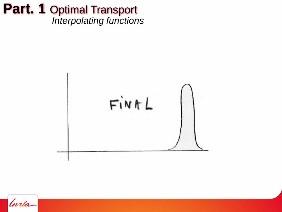
Part. 1 Optimal TransportInterpolating functions
Part. 1 Optimal TransportInterpolating functions

Part. 1 Optimal TransportInterpolating functions

Part. 1 Optimal TransportInterpolating functions

Part. 1 Optimal TransportInterpolating functions

Part. 1 Optimal TransportInterpolating functions

Part. 1 Optimal TransportInterpolating functions

Part. 1 Optimal TransportInterpolating functions

Part. 1 Optimal TransportInterpolating functions

Part. 1 Optimal TransportInterpolating functions

Part. 1 Optimal TransportInterpolating functions

Part. 1 Optimal TransportInterpolating functions

Part. 1 Optimal Transport
?
T

Part. 1 Optimal Transport
?
T
distance between the shapes

Part. 1 Optimal Transport
while preserving mass and minimizing the effort ?
?
T

Part. 1 Optimal Transport
while preserving mass and minimizing the effort ?
?
T

Part. 1 Optimal Transport
while preserving mass and minimizing the effort ?
?
T

Part. 1 Optimal Transport
OT=
Yann Brenier:
it can be replaced with the Monge-Ampère

Part. 1 Optimal Transport
OT=
Yann Brenier:
it can be replaced with the Monge-Ampère
New ways of simulating physics with a computer

Part. 1 Optimal Transport
OT=
Yann Brenier:
Laplace operator is used in a PDE,
it can be replaced with the Monge-Ampère
New ways of simulating physics with a computer
Fast Fourier Transform
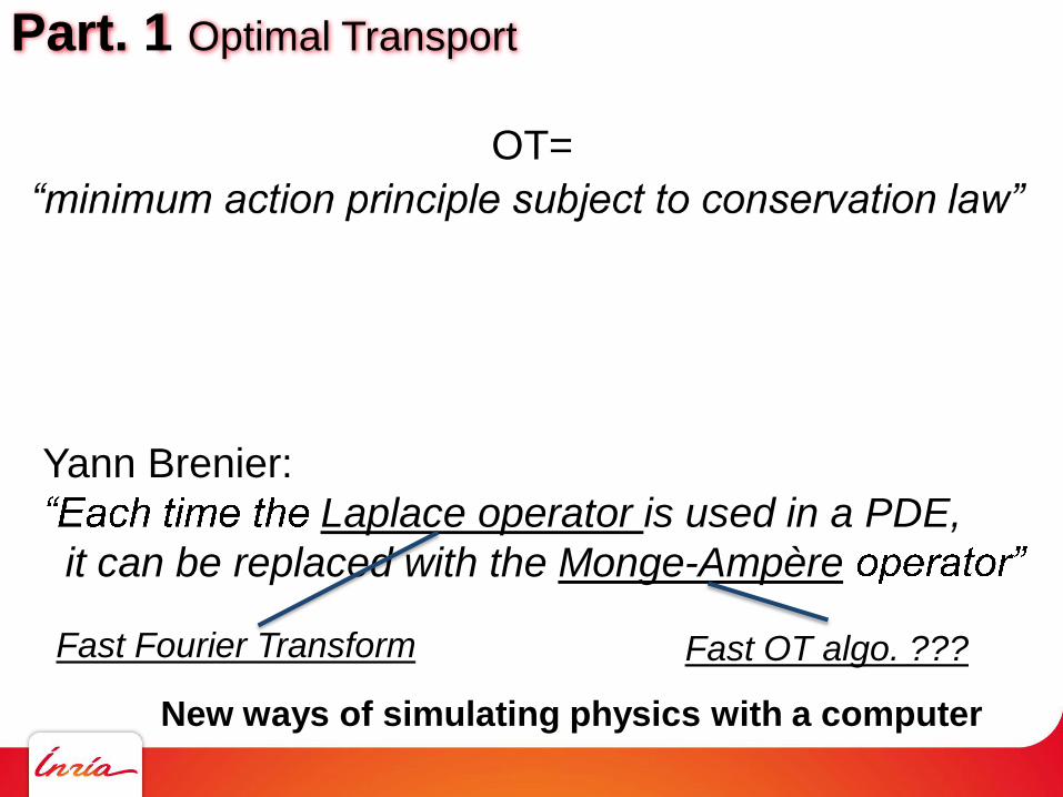
Part. 1 Optimal Transport
OT=
Yann Brenier:
Laplace operator is used in a PDE,
it can be replaced with the Monge-Ampère
New ways of simulating physics with a computer
Fast Fourier Transform Fast OT algo. ???

Part. 1 Optimal Transport
Gaspard Monge - 1784

Part. 1 Optimal Transport
Gaspard Monge geometry and light
ANR TOMMI Workshop

Part. 1 Optimal Transport
[Castro, Merigot, Thibert 2014]
Optimal transport
geometry and light
[Caffarelli, Kochengin, and Oliker 1999]

Part. 1 Optimal Transport Image Processing
Barycenters / mixing textures Video-style transfer
[Nicolas Bonneel, Julien Rabin, Gabriel
Peyre, Hanspeter Pfister][Nicolas Bonneel, Kalyan Sunkavalli, Sylvain
Paris, Hanspeter Pfister]

Part. 1 Optimal Transport
Optimal transport - geometry and light
[Chwartzburg, Testuz, Tagliasacchi, Pauly, SIGGRAPH 2014]

Part. 1. Motivations
Discretization of functionals involving the Monge-Ampère operator,
Benamou, Carlier, Mérigot, Oudet
arXiv:1408.4536
The variational formulation of the Fokker-Planck equation
Jordan, Kinderlehrer and Otto
SIAM J. on Mathematical Analysis
Geostrophic current

Part. 1 Optimal Transport
Optimal transport E.U.R.
The data

Part. 1 Optimal Transport
The millenium simulation project, Max Planck Institute fur Astrophysik
pc/h : parsec (= 3.2 light years)

Part. 1 Optimal Transport
Optimal transport E.U.R.
The universal swimming pool
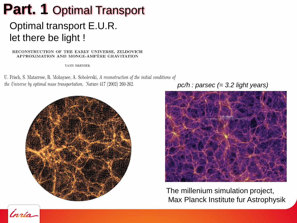
Part. 1 Optimal Transport
Optimal transport E.U.R.
let there be light !
The millenium simulation project,
Max Planck Institute fur Astrophysik
pc/h : parsec (= 3.2 light years)

Part. 1 Optimal Transport
Optimal transport E.U.R.
let there be light !
The millenium simulation project,
Max Planck Institute fur Astrophysik
pc/h : parsec (= 3.2 light years)
In 2002: 5 hours of computation
on a super-computer for 5000 points
with a O(n3) algorithm.

Part. 1 Optimal Transport
Optimal transport E.U.R.
let there be light !
The millenium simulation project,
Max Planck Institute fur Astrophysik
pc/h : parsec (= 3.2 light years)
In 2002: 5 hours of computation
on a super-computer for 5000 points
with a O(n3) algorithm.
Can we do the computation with
1 000 000 points ?

Optimal Transportan elementary introduction
2

Part. 2 Optimal Transport problem
(X; ) (Y; )
Two measures , such that d (x) = d (x)X Y

Part. 2 Optimal Transport problem
A map T is a transport map between and if
(T-1(B)) = (B) for any Borel subset B of Y
(X; ) (Y; )

Part. 2 Optimal Transport problem
A map T is a transport map between and if
(T-1(B)) = (B) for any Borel subset B
B
(X; ) (Y; )

Part. 2 Optimal Transport problem
A map T is a transport map between and if
(T-1(B)) = (B) for any Borel subset B
BT-1(B)
(X; ) (Y; )

Part. 2 Optimal Transport problem
A map T is a transport map between and if
(T-1(B)) = (B) for any Borel subset B
(or = T# the pushforward of )
(X; ) (Y; )

Part. 2 Optimal Transport problem
problem:
Find a transport map T that minimizes C(T) = X || x T(x) ||2 d (x)
(X; ) (Y; )

Part. 2 Optimal Transport problem
problem:
Find a transport map T that minimizes C(T) = X || x T(x) ||2 d (x)
Difficult to study
If has an atom (isolated Dirac),
it can only be mapped to another Dirac
(T needs to be a map)

Part. 2 Optimal Transport problem
problem:
Find a transport map T that minimizes C(T) = X || x T(x) ||2 d (x)
Transport from a measure concentrated on L1 onto another one concentrated on L2 and L3

Part. 2 Optimal Transport problem
problem:
Find a transport map T that minimizes C(T) = X || x T(x) ||2 d (x)
Transport from a measure concentrated on L1 onto another one concentrated on L2 and L3

Part. 2 Optimal Transport problem
problem:
Find a transport map T that minimizes C(T) = X || x T(x) ||2 d (x)
Transport from a measure concentrated on L1 onto another one concentrated on L2 and L3

Part. 2 Optimal Transport problem
problem:
Find a transport map T that minimizes C(T) = X || x T(x) ||2 d (x)
Transport from a measure concentrated on L1 onto another one concentrated on L2 and L3
The infimum is never realized by a map, need for a relaxation
Part. 2 Optimal Transport Kantorovich
problem:
Find a transport map T that minimizes C(T) = X || x T(x) ||2 d (x)
(1942):
Find a measure defined on X x Y
such that x in X d (x,y) = d (y)
and y in Y d (x,y) = d (x)
that minimizes X x Y || x y ||2 d (x,y)

Part. 2 Optimal Transport Kantorovich
problem:
Find a transport map T that minimizes C(T) = X || x T(x) ||2 d (x)
Find a measure defined on X x Y
such that x in X d (x,y) = d (y)
and y in Y d (x,y) = d (x)
that minimizes X x Y || x y ||2 d (x,y)
(x,y
How much sand goes from x to y

Part. 2 Optimal Transport Kantorovich
problem:
Find a transport map T that minimizes C(T) = X || x T(x) ||2 d (x)
Find a measure defined on X x Y
such that x in X d (x,y) = d (y)
and y in Y d (x,y) = d (x)
that minimizes X x Y || x y ||2 d (x,y)
Everything that is
transported from x

Part. 2 Optimal Transport Kantorovich
problem:
Find a transport map T that minimizes C(T) = X || x T(x) ||2 d (x)
Find a measure defined on X x Y
such that x in X d (x,y) = d (y)
and y in Y d (x,y) = d (x)
that minimizes X x Y || x y ||2 d (x,y)
Everything that is
transported to y

Part. 2 Optimal Transport Kantorovich
Transport plan example 1/4 : translation of a segment

Part. 2 Optimal Transport Kantorovich
Transport plan example 1/4 : translation of a segment

Part. 2 Optimal Transport Kantorovich
Transport plan example 2/4 : spitting a segment
Part. 2 Optimal Transport Kantorovich

Part. 2 Optimal Transport Kantorovich

Part. 2 Optimal Transport Kantorovich

Part. 2 Optimal Transport Kantorovich
Transport plan example 3/4 : splitting a Dirac into two Diracs

Part. 2 Optimal Transport Kantorovich
Transport plan example 3/4 : splitting a Dirac into two Diracs
(No transport map)

Part. 2 Optimal Transport Kantorovich
Transport plan example 4/4 : splitting a Dirac into two segments

Part. 2 Optimal Transport Kantorovich
Transport plan example 4/4 : splitting a Dirac into two segments
(No transport map)

Part. 2 Optimal Transport Duality

Part. 2 Optimal Transport Duality
Duality is easier to understand with a discrete version

Part. 2 Optimal Transport Duality(DMK):
Min <c, >
P1 = u
s.t. P2 = v

Part. 2 Optimal Transport Duality(DMK):
Min <c, >
P1 = u
s.t. P2 = v
=
11
12
1n
22
2n
mn
IRmn

Part. 2 Optimal Transport Duality(DMK):
Min <c, >
P1 = u
s.t. P2 = v
=
11
12
1n
22
2n
mn
c =
c11
c12
c1n
c22
c2n
cmn
IRmnIRmn

Part. 2 Optimal Transport Duality(DMK):
Min <c, >
P1 = u
s.t. P2 = v
=
11
12
1n
22
2n
mn
c =
c11
c12
c1n
c22
c2n
cmncij = || xi yj ||2
IRmnIRmn
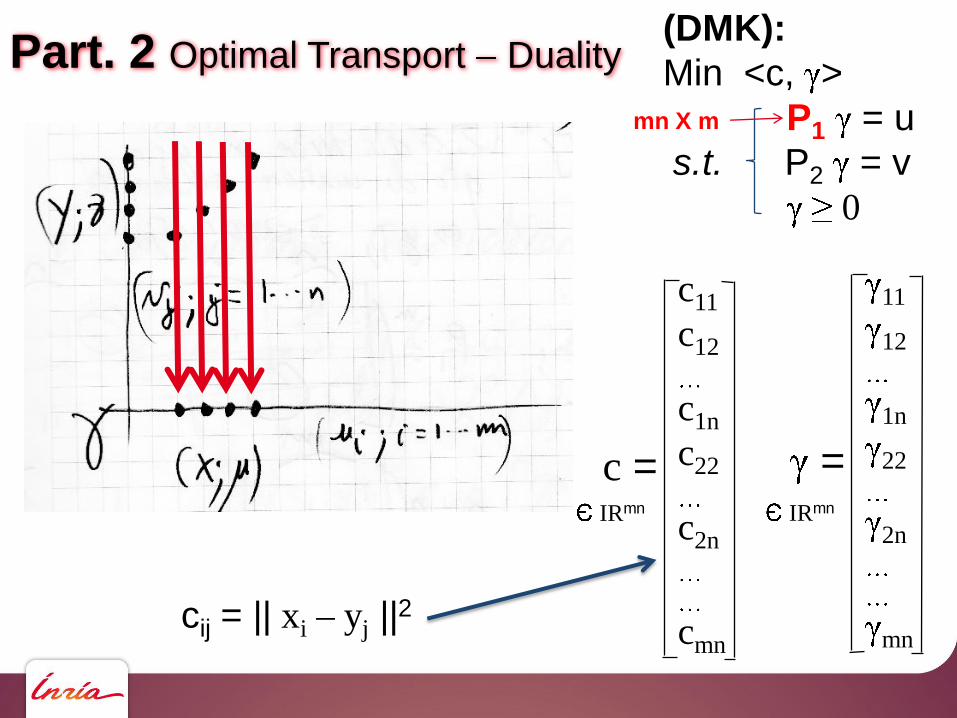
Part. 2 Optimal Transport Duality(DMK):
Min <c, >
P1 = u
s.t. P2 = v
0
=
11
12
1n
22
2n
mn
c =
c11
c12
c1n
c22
c2n
cmncij = || xi yj ||2
mn X m
IRmnIRmn

Part. 2 Optimal Transport Duality(DMK):
Min <c, >
P1 = u
s.t. P2 = v
=
11
12
1n
22
2n
mn
c =
c11
c12
c1n
c22
c2n
cmncij = || xi yj ||2
mn X n
mn X m
IRmnIRmn

Part. 2 Optimal Transport Duality(DMK):
Min <c, >
P1 = u
s.t. P2 = v
=
11
12
1n
22
2n
mn
c =
c11
c12
c1n
c22
c2n
cmn
IRmnIRmn
mn X n
mn X m

Part. 2 Optimal Transport Duality
Consider L( , ) = <c, > - < , P1 - u> - < , P2 - v>
(DMK):
Min <c, >
P1 = u
s.t. P2 = v< u, v > denotes the dot product between u and v

Part. 2 Optimal Transport Duality
Consider L( , ) = <c, > - < , P1 - u> - < , P2 - v>
Remark: Sup[ L( , ) ] = < c, > if P1 = u and P2 = v IRm
IRn
(DMK):
Min <c, >
P1 = u
s.t. P2 = v

Part. 2 Optimal Transport Duality
Consider L( , ) = <c, > - < , P1 - u> - < , P2 - v>
Remark: Sup[ L( , ) ] = < c, > if P1 = u and P2 = v IRm
IRn
(DMK):
Min <c, >
P1 = u
s.t. P2 = v
0

Part. 2 Optimal Transport Duality
Consider L( , ) = <c, > - < , P1 - u> - < , P2 - v>
Remark: Sup[ L( , ) ] = < c, > if P1 = u and P2 = v IRm
IRn
Consider now: Inf [ Sup[ L( , ) ] ]IRm
IRn
(DMK):
Min <c, >
P1 = u
s.t. P2 = v

Part. 2 Optimal Transport Duality
Consider L( , ) = <c, > - < , P1 - u> - < , P2 - v>
Remark: Sup[ L( , ) ] = < c, > if P1 = u and P2 = v IRm
IRn
Consider now: Inf [ Sup[ L( , ) ] ] = Inf [ < c, > ] IRm
IRn P1 = u
P2 = v
(DMK):
Min <c, >
P1 = u
s.t. P2 = v

Part. 2 Optimal Transport Duality
Consider L( , ) = <c, > - < , P1 - u> - < , P2 - v>
Remark: Sup[ L( , ) ] = < c, > if P1 = u and P2 = v IRm
IRn
Consider now: Inf [ Sup[ L( , ) ] ] = Inf [ < c, > ] (DMK)IRm
IRn0
P1 = u
P2 = v
(DMK):
Min <c, >
P1 = u
s.t. P2 = v

Part. 2 Optimal Transport Duality
IRm
IRn
Inf [ Sup[ <c, > - < , P1 - u> - < , P2 - v> ] ]
(DMK):
Min <c, >
P1 = u
s.t. P2 = v

Part. 2 Optimal Transport Duality
IRm
IRn0
Inf [ Sup[ <c, > - < , P1 - u> - < , P2 - v> ] ]
IRm
IRn
Sup[ Inf[ <c, > - < , P1 - u> - < , P2 - v> ] ]
Exchange Inf Sup
(DMK):
Min <c, >
P1 = u
s.t. P2 = v

Part. 2 Optimal Transport Duality
IRm
IRn
Inf [ Sup[ <c, > - < , P1 - u> - < , P2 - v> ] ]
IRm
IRn
Sup[ Inf[ <c, > - < , P1 - u> - < , P2 - v> ] ]
IRm
IRn
0
Sup[ Inf[ < ,c-P1t P2
t > + < ,u> + < , v> ] ]
Exchange Inf Sup
Expand/Reorder/Collect
(DMK):
Min <c, >
P1 = u
s.t. P2 = v
0

Part. 2 Optimal Transport Duality
IRm
IRn
Inf [ Sup[ <c, > - < , P1 - u> - < , P2 - v> ] ]
IRm
IRn
Sup[ Inf[ <c, > - < , P1 - u> - < , P2 - v> ] ]
IRm
IRn
Sup[ Inf[ < ,c-P1t P2
t > + < ,u> + < , v> ] ]
Exchange Inf Sup
Expand/Reorder/Collect
Interpret
(DMK):
Min <c, >
P1 = u
s.t. P2 = v

Part. 2 Optimal Transport Duality
IRm
IRn
Sup[ Inf[ < ,c-P1t P2
t > + < ,u> + < , v> ] ]
Interpret
Sup[ < ,u> + < , v> ] IRm
IRn
P1t + P2
t c
(DMK):
Min <c, >
P1 = u
s.t. P2 = v
(DDMK)

Part. 2 Optimal Transport Duality
IRm
IRn
Sup[ Inf[ < ,c-P1t P2
t > + < ,u> + < , v> ] ]
Interpret
Sup[ < ,u> + < , v> ] IRm
IRn
P1t + P2
t c i + j cij (i,j)
A
(DMK):
Min <c, >
P1 = u
s.t. P2 = v
(DDMK)

Part. 2 Optimal Transport Kantorovich dual
Find a measure defined on X x Y
such that x in X d (x,y) = d (x)
and y in Y d (x,y) = d (x)
that minimizes X x Y || x y ||2 d (x,y)
Find two functions in L1( ) and in L1( )
Such that for all x,y, (x) + y ||2
that maximize X d + Y d

Part. 2 Optimal Transport Kantorovich dual
Find a measure defined on X x Y
such that x in X d (x,y) = d (x)
and y in Y d (x,y) = d (x)
that minimizes X x Y || x y ||2 d (x,y)
Find two functions in L1( ) and in L1( )
Such that for all x,y, (x) + y ||2
that maximize X d + Y d
Your point of view:
Try to minimize transport cost

Part. 2 Optimal Transport Kantorovich dual
Find a measure defined on X x Y
such that x in X d (x,y) = d (x)
and y in Y d (x,y) = d (x)
that minimizes X x Y || x y ||2 d (x,y)
Find two functions in L1( ) and in L1( )
Such that for all x,y, (x) + y ||2
that maximize X d + Y d Try to maximize transport price
Your point of view:
Try to minimize transport cost

Part. 2 Optimal Transport Kantorovich dual
Find a measure defined on X x Y
such that x in X d (x,y) = d (x)
and y in Y d (x,y) = d (x)
that minimizes X x Y || x y ||2 d (x,y)
Find two functions in L1( ) and in L1( )
Such that for all x,y, (x) + y ||2
that maximize X (x)d + Y (y)d
What they charge for loading at x
Your point of view:
Try to minimize transport cost

Part. 2 Optimal Transport Kantorovich dual
Find a measure defined on X x Y
such that x in X d (x,y) = d (x)
and y in Y d (x,y) = d (x)
that minimizes X x Y || x y ||2 d (x,y)
Find two functions in L1( ) and in L1( )
Such that for all x,y, (x) + y ||2
that maximize X (x)d + Y (y)d
What they charge for loading at x What they charge for unloading at y
Price (loading + unloading) cannot
be greater than transport cost
(else you do the job yourself)
Your point of view:
Try to minimize transport cost

Part. 2 Optimal Transport c-conjugate functions
Find two functions in L1( ) and in L1( )
Such that for all x,y, (x) + y ||2
that maximize X (x)d + Y (y)d

Part. 2 Optimal Transport c-conjugate functions
Find two functions in L1( ) and in L1( )
Such that for all x,y, (x) + y ||2
that maximize X (x)d + Y (y)d
If we got two functions and that satisfy the constraint
Then it is possible to obtain a better solution by replacing with c defined by:
For all y, c(y) = inf x in X ½|| x y ||2 - (y)
c is called the c-conjugate function of
If there is a function such that = c then is said to be c-concave
If is c-concave, then cc =

Part. 2 Optimal Transport c-conjugate functions
Find a c-concave function
that maximizes X (x)d + Yc(y)d

Part. 2 Optimal Transport c-conjugate functions
Find a c-concave function
that maximizes X (x)d + Yc(y)d
is called a

Part. 2 Optimal Transport c-subdifferential
What about our initial problem ?
is called a
Find a c-concave function
that maximizes X (x)d + Yc(y)d

Part. 2 Optimal Transport c-subdifferential
is called a
Find a c-concave function
that maximizes X (x)d + Yc(y)d

Part. 2 Optimal Transport c-subdifferential

Part. 2 Optimal Transport c-subdifferential
Proof: see OTON, chap. 10.

Part. 2 Optimal Transport c-subdifferential
Proof: see OTON, chap. 10.
Heuristic argument (at the beginning of the same chapter):

Part. 2 Optimal Transport c-subdifferential
Proof: see OTON, chap. 10.
Heuristic argument (at the beginning of the same chapter):

Part. 2 Optimal Transport c-subdifferential
Proof: see OTON, chap. 10.
Heuristic argument (at the beginning of the same chapter):

Part. 2 Optimal Transport c-subdifferential
Proof: see OTON, chap. 10.
Heuristic argument (at the beginning of the same chapter):

Part. 2 Optimal Transport c-subdifferential
Proof: see OTON, chap. 10.
Heuristic argument (at the beginning of the same chapter):

Part. 2 Optimal Transport c-subdifferential
Proof: see OTON, chap. 10.
Heuristic argument (at the beginning of the same chapter):

Part. 2 Optimal Transport c-subdifferential
Proof: see OTON, chap. 10.
Heuristic argument (at the beginning of the same chapter):
w

Part. 2 Optimal Transport c-subdifferential
Proof: see OTON, chap. 10.
Heuristic argument (at the beginning of the same chapter):
-w

Part. 2 Optimal Transport c-subdifferential
Find a c-concave function
that maximizes X (x)d + Yc(y)d

Part. 2 Optimal Transport c-subdifferential
Find a c-concave function
that maximizes X (x)d + Yc(y)d
{
grad (x) with (x) := (½ x2- (x))

Part. 2 Optimal Transport convexity
Find a c-concave function
that maximizes X (x)d + Yc(y)d
{
grad (x) with (x) := (½ x2- (x))
is convex

Part. 2 Optimal Transport convexity
Find a c-concave function
that maximizes X (x)d + Yc(y)d
{
grad (x) with (x) := (½ x2- (x))
is convex

Part. 2 Optimal Transport convexity
Find a c-concave function
that maximizes X (x)d + Yc(y)d
{
grad (x) with (x) := (½ x2- (x))
is convex
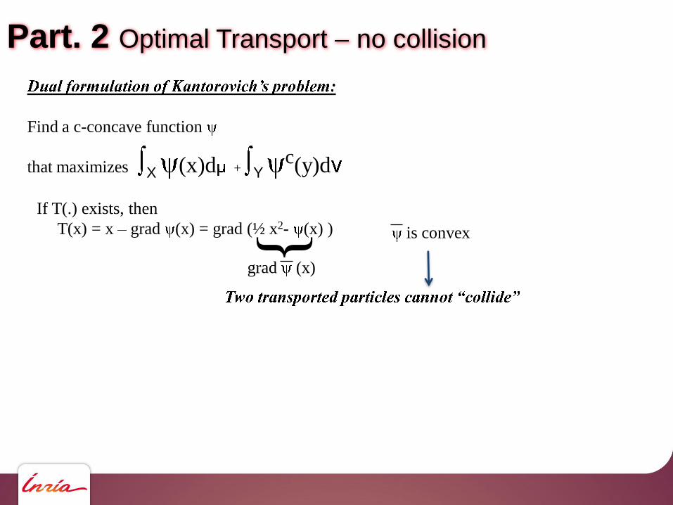
Part. 2 Optimal Transport no collision
If T(.) exists, then
T(x) = x grad (x) = grad (½ x2- (x) ) {grad (x)
Find a c-concave function
that maximizes X (x)d + Yc(y)d
is convex

Part. 2 Optimal Transport no collision
If T(.) exists, then
T(x) = x grad (x) = grad (½ x2- (x) ) {grad (x)
Find a c-concave function
that maximizes X (x)d + Yc(y)d
is convex

Part. 2 Optimal Transport no collision
If T(.) exists, then
T(x) = x grad (x) = grad (½ x2- (x) ) {grad (x)
Find a c-concave function
that maximizes X (x)d + Yc(y)d
is convex

Part. 2 Optimal Transport Monge-Ampere
What about our initial problem ? If T(.) exists, then one can show that:
T(x) = x grad (x) = grad (½ x2- (x) ) {
for all borel set A, A d = T(A) (|JT|) d (change of variable)
Jacobian of T (1st order derivatives)
Find a c-concave function
that maximizes X (x)d + Yc(y)d
grad (x) with (x) := (½ x2- (x))

Part. 2 Optimal Transport Monge-Ampere
What about our initial problem ? If T(.) exists, then one can show that:
T(x) = x grad (x) = grad (½ x2- (x) ) {
for all borel set A, A d = T(A) (|JT|) d = T(A) (H ) d
Det. of the Hessian of (2nd order derivatives)
Find a c-concave function
that maximizes X (x)d + Yc(y)d
grad (x) with (x) := (½ x2- (x))

Part. 2 Optimal Transport Monge-Ampere
What about our initial problem ?
T(x) = x grad (x) = grad (½ x2- (x) ) {
grad (x) with (x) := (½ x2- (x))
When and have a density u and v, (H (x)). v(grad (x)) = u(x)Monge-Ampère
equation
for all borel set A, A d = T(A) (|JT|) d = T(A) (H ) d
Find a c-concave function
that maximizes X (x)d + Yc(y)d

Part. 2 Optimal Transport summary
Find a transport map T that minimizes C(T) = X || x T(x) ||2 d (x)

Part. 2 Optimal Transport summary
Find a transport map T that minimizes C(T) = X || x T(x) ||2 d (x)
(Kantorovich formulation, dual, c-convex functions)

Part. 2 Optimal Transport summary
Find a transport map T that minimizes C(T) = X || x T(x) ||2 d (x)
(Kantorovich formulation, dual, c-convex functions)
Monge-Ampère equation (When and have a density u and v resp.)
Solve (H (x)). v(grad (x)) = u(x)

Part. 2 Optimal Transport summary
Find a transport map T that minimizes C(T) = X || x T(x) ||2 d (x)
(Kantorovich formulation, dual, c-convex functions)
Brenier, Mc Cann, Trudinger: The optimal transport map is then given by:
T(x) = grad (x)
Solve (H (x)). v(grad (x)) = u(x) Monge-Ampère equation (When and have a density u and v resp.)
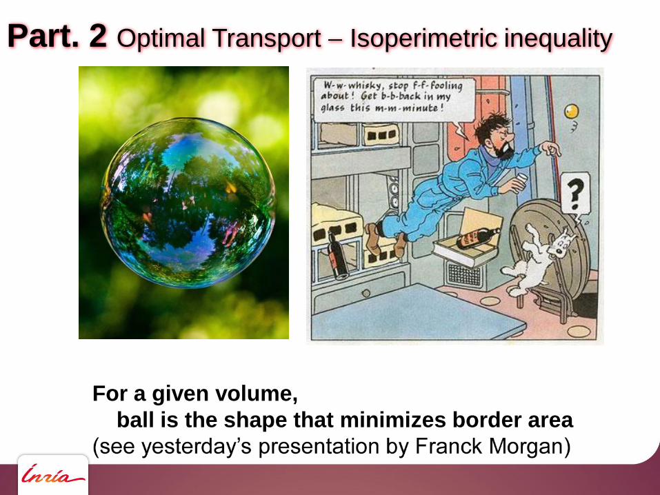
Part. 2 Optimal Transport Isoperimetric inequality
For a given volume,
ball is the shape that minimizes border area
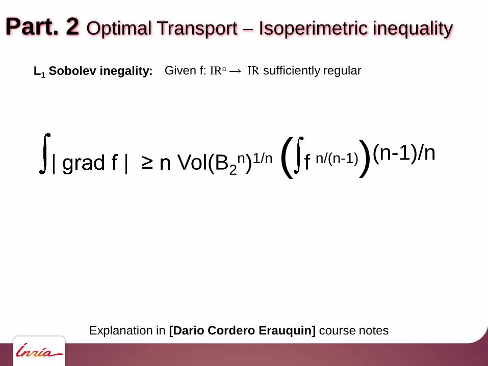
Part. 2 Optimal Transport Isoperimetric inequality
Vol(B2n)1/n ( f n/(n-1))(n-1)/n
L1 Sobolev inegality: Given f: IRn sufficiently regular
Explanation in [Dario Cordero Erauquin] course notes

Part. 2 Optimal Transport Isoperimetric inequality
n Vol(B2n)1/n ( f n/(n-1))(n-1)/n
L1 Sobolev inegality: Given f: IRn sufficiently regular
Explanation in [Dario Cordero Erauquin] course notes

Part. 2 Optimal Transport Isoperimetric inequality
Vol(B2n)1/n ( f n/(n-1))(n-1)/n
L1 Sobolev inegality: Given f: IRn sufficiently regular
Explanation in [Dario Cordero Erauquin] course notes

Part. 2 Optimal Transport Isoperimetric inequality
Vol(B2n)1/n ( f n/(n-1))(n-1)/n
L1 Sobolev inegality: Given f: IRn sufficiently regular
Consider a compact set such that Vol( ) = Vol(B23)
and f = the indicatrix function of

Part. 2 Optimal Transport Isoperimetric inequality
Vol(B2n)1/n ( f n/(n-1))(n-1)/n
L1 Sobolev inegality: Given f: IRn sufficiently regular
Consider a compact set such that Vol( ) = Vol(B23)
and f = the indicatrix function of
Vol Vol(B23)1/3 Vol(B2
3)2/3

Part. 2 Optimal Transport Isoperimetric inequality
Vol(B2n)1/n ( f n/(n-1))(n-1)/n
L1 Sobolev inegality: Given f: IRn sufficiently regular
Consider a compact set such that Vol( ) = Vol(B23)
and f = the indicatrix function of
Vol Vol(B23)1/3 Vol(B2
3)2/3
Vol = Vol 23)

Part. 2 Optimal Transport Isoperimetric inequality
Vol(B2n)1/n ( f n/(n-1))(n-1)/n
L1 Sobolev inegality: a proof with OT [Gromov]

Part. 2 Optimal Transport Isoperimetric inequality
Vol(B2n)1/n ( f n/(n-1))(n-1)/n
L1 Sobolev inegality: a proof with OT [Gromov]
We suppose w.l.o.g. that f n/(n-1) = 1

Part. 2 Optimal Transport Isoperimetric inequality
Vol(B2n)1/n ( f n/(n-1))(n-1)/n
L1 Sobolev inegality: a proof with OT [Gromov]
There exists an optimal transport T = grad between
f n/(n-1)(x)dx and 1B2n/Vol(B2
n)dx
We suppose w.l.o.g. that f n/(n-1) = 1

Part. 2 Optimal Transport Isoperimetric inequality
Vol(B2n)1/n ( f n/(n-1))(n-1)/n
L1 Sobolev inegality: a proof with OT [Gromov]
There exists an optimal transport T = grad between
f n/(n-1)(x)dx and 1B2n/Vol(B2
n)dx
We suppose w.l.o.g. that f n/(n-1) = 1
Monge-Ampère equation: Vol(B2n) fn/(n-1)(x) = det Hess
Arithmetico-geometric ineq: det (H) 1/n
det (Hess ) 1/n )/n
det (Hess ) 1/n / n

Part. 2 Optimal Transport Isoperimetric inequality
Vol(B2n)1/n ( f n/(n-1))(n-1)/n
L1 Sobolev inegality: a proof with OT [Gromov]
We suppose w.l.o.g. that f n/(n-1) = 1
det (Hess ) 1/n )/nMonge-Ampère equation:
Vol(B2n) fn/(n-1)(x) = det Hess

Part. 2 Optimal Transport Isoperimetric inequality
Vol(B2n)1/n ( f n/(n-1))(n-1)/n
L1 Sobolev inegality: a proof with OT [Gromov]
We suppose w.l.o.g. that f n/(n-1) = 1
Vol(B2n) = Vol(B2
n) f n/(n-1) = f Vol(B2n) f 1/(n-1)
det (Hess ) 1/n )/nMonge-Ampère equation:
Vol(B2n) fn/(n-1)(x) = det Hess

Part. 2 Optimal Transport Isoperimetric inequality
Vol(B2n)1/n ( f n/(n-1))(n-1)/n
L1 Sobolev inegality: a proof with OT [Gromov]
We suppose w.l.o.g. that f n/(n-1) = 1
Vol(B2n) = Vol(B2
n) f n/(n-1) = f Vol(B2n) f 1/(n-1)
det (Hess ) 1/n )/nMonge-Ampère equation:
Vol(B2n) fn/(n-1)(x) = det Hess

Part. 2 Optimal Transport Isoperimetric inequality
Vol(B2n)1/n ( f n/(n-1))(n-1)/n
L1 Sobolev inegality: a proof with OT [Gromov]
We suppose w.l.o.g. that f n/(n-1) = 1
Vol(B2n) = Vol(B2
n) f n/(n-1) = f Vol(B2n) f 1/(n-1)
= - grad f . grad
det (Hess ) 1/n )/nMonge-Ampère equation:
Vol(B2n) fn/(n-1)(x) = det Hess

Part. 2 Optimal Transport Isoperimetric inequality
Vol(B2n)1/n ( f n/(n-1))(n-1)/n
L1 Sobolev inegality: a proof with OT [Gromov]
We suppose w.l.o.g. that f n/(n-1) = 1
Vol(B2n) = Vol(B2
n) f n/(n-1) = f Vol(B2n) f 1/(n-1) 1/n
= - grad f . grad | grad f | (T = grad B2n )
det (Hess ) 1/n )/nMonge-Ampère equation:
Vol(B2n) fn/(n-1)(x) = det Hess

Part. 2 Optimal Transport Isoperimetric inequality
Vol(B2n)1/n ( f n/(n-1))(n-1)/n
L1 Sobolev inegality: a proof with OT [Gromov]
We suppose w.l.o.g. that f n/(n-1) = 1
Vol(B2n) = Vol(B2
n) f n/(n-1) = f Vol(B2n) f 1/(n-1)
= - grad f . grad | grad f | (T = grad B2n )
Vol(B2n)1/n
det (Hess ) 1/n )/nMonge-Ampère equation:
Vol(B2n) fn/(n-1)(x) = det Hess

Semi-Discrete Optimal Transport
3

Part. 3 Optimal Transport how to program ?
Continuous
(X; ) (Y; )

Part. 3 Optimal Transport how to program ?
Continuous
Semi-discrete
(X; ) (Y; )

Part. 3 Optimal Transport how to program ?
Continuous
Semi-discrete
Discrete
(X; ) (Y; )

Part. 3 Optimal Transport how to program ?
Continuous
Semi-discrete
Discrete
(X; ) (Y; )

Part. 3 Optimal Transport semi-discrete
Xc (x)d + Y (y)d
Supc
(DMK)
(X; ) (Y; )

Part. 3 Optimal Transport semi-discrete (X; ) (Y; )
j (yj) vj
Xc (x)d + Y (y)d
Supc
(DMK)

Part. 3 Optimal Transport semi-discrete
Xc (x)d + Y (y)d
Supc
(DMK)
j (yj) vj

Part. 3 Optimal Transport semi-discrete
Xc (x)d + Y (y)d
Supc
(DMK)
X inf yj Y [ || x yj ||2 - (yj) ] d
j (yj) vj

Part. 3 Optimal Transport semi-discrete
Xc (x)d + Y (y)d
Supc
(DMK)
j Lag (yj) || x yj ||2 - (yj) d
X inf yj Y [ || x yj ||2 - (yj) ] d
j (yj) vj

Part. 3 Optimal Transport semi-discrete
G( ) = j Lag (yj) || x yj ||2 - (yj) d + j (yj) vjSup
c
(DMK)
Where: Lag (yj) = { x | || x yj ||2 (yj) < || x yj ||2 - (yj ) }

Part. 3 Optimal Transport semi-discrete
G( ) = j Lag (yj) || x yj ||2 - (yj) d + j (yj) vjSup
c
(DMK)
Where: Lag (yj) = { x | || x yj ||2 (yj) < || x yj ||2 - (yj ) }
Laguerre diagram of the yj
(with the L2 cost || x y ||2 used here, Power diagram)

Part. 3 Optimal Transport semi-discrete
G( ) = j Lag (yj) || x yj ||2 - (yj) d + j (yj) vjSup
c
(DMK)
Where: Lag (yj) = { x | || x yj ||2 (yj) < || x yj ||2 - (yj ) }
Laguerre diagram of the yj
(with the L2 cost || x y ||2 used here, Power diagram)
Weight of yj in the power diagram

Part. 3 Optimal Transport semi-discrete
G( ) = j Lag (yj) || x yj ||2 - (yj) d + j (yj) vjSup
c
(DMK)
Where: Lag (yj) = { x | || x yj ||2 (yj) < || x yj ||2 - (yj ) }
Laguerre diagram of the yj
(with the L2 cost || x y ||2 used here, Power diagram)
Weight of yj in the power diagram
is determined by the
weight vector [ (y1) (y2 (ym)]
For all weight vector, is c-concave

Voronoi diagram: Vor(xi) = { x | d2(x,xi) < d2(x,xj) }
Part. 3 Power Diagrams

Power diagram: Pow(xi) = { x | d2(x,xi) i < d2(x,xj) j }
Voronoi diagram: Vor(xi) = { x | d2(x,xi) < d2(x,xj) }
Part. 3 Power Diagrams

Part. 3 Power Diagrams

Part. 3 Optimal Transport
Theorem: (direct consequence of MK duality
alternative proof in [Aurenhammer, Hoffmann, Aronov 98] ):
Given a measure with density, a set of points (yj), a set of positive coefficients vj
such that vj d (x), it is possible to find the weights W = [ (y1) (y2 (ym)]
such that the map TSW is the unique optimal transport map
between and = vj (yj)
Proof: G( ) = j Lag (yj) || x yj ||2 - (yj) d + j (yj) vj
Is a concave function of the weight vector [ (y1) (y2 (ym)]

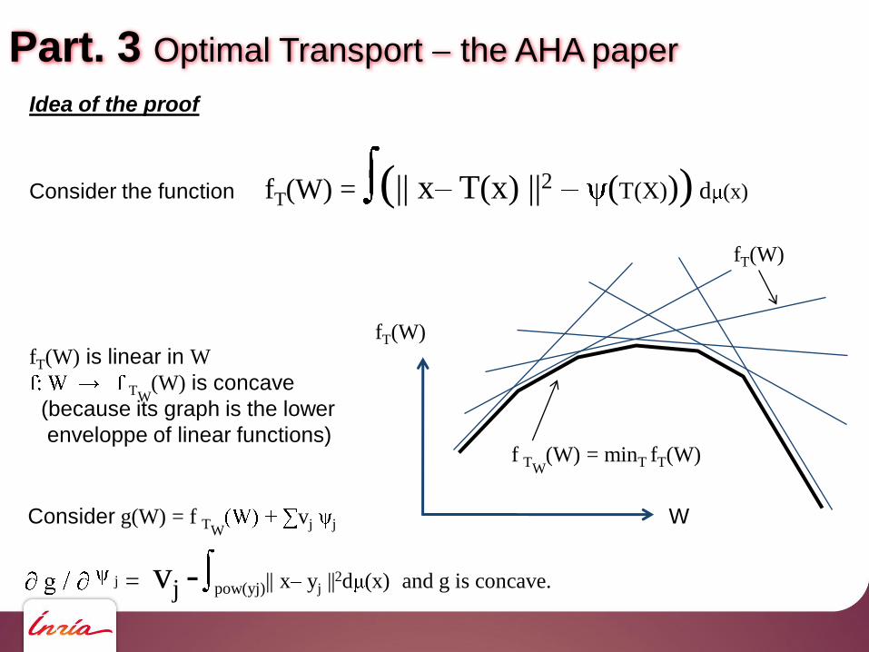
Part. 3 Optimal Transport the AHA paper
Idea of the proof
Consider the function fT(W) = (|| x T(x) ||2 (T(X))) d (x)
The (unknown) weights W = [ (y1) (y2 (ym)]

Part. 3 Optimal Transport the AHA paper
Idea of the proof
Consider the function fT(W) = (|| x T(x) ||2 (T(X))) d (x)
T : an arbitrary but fixed assignment.

Part. 3 Optimal Transport the AHA paper
Idea of the proof
Consider the function fT(W) = (|| x T(x) ||2 (T(X))) d (x)
T : an arbitrary but fixed assignment.

Part. 3 Optimal Transport the AHA paper
Idea of the proof
Consider the function fT(W) = (|| x T(x) ||2 (T(X))) d (x)
T : an arbitrary but fixed assignment.

Part. 3 Optimal Transport the AHA paper
Idea of the proof
Consider the function fT(W) = (|| x T(x) ||2 (T(X))) d (x)
T : an arbitrary but fixed assignment.

Part. 3 Optimal Transport the AHA paper
Idea of the proof
Consider the function fT(W) = (|| x T(x) ||2 (T(X))) d (x)
W
fT(W)
fT(W)

Part. 3 Optimal Transport the AHA paper
Idea of the proof
Consider the function fT(W) = (|| x T(x) ||2 (T(X))) d (x)
W
fT(W)
fT(W)

Part. 3 Optimal Transport the AHA paper
Idea of the proof
Consider the function fT(W) = (|| x T(x) ||2 (T(X))) d (x)
fT(W) is linear in W
fT(W)
W
fT(W)
Fixed T

Part. 3 Optimal Transport the AHA paper
Idea of the proof
Consider the function fT(W) = (|| x T(x) ||2 (T(X))) d (x)
fT(W) is linear in W
f TW
(W) : defined by power diagram
fT(W)
fixed WW

Part. 3 Optimal Transport the AHA paper
Idea of the proof
Consider the function fT(W) = (|| x T(x) ||2 (T(X))) d (x)
fT(W) is linear in W
f TW(W) = minT fT(W)
fT(W)
fixed WW

Part. 3 Optimal Transport the AHA paper
Idea of the proof
Consider the function fT(W) = (|| x T(x) ||2 (T(X))) d (x)
fT(W) is linear in W
TW(W) is concave !!
(because its graph is the lower
enveloppe of linear functions)
fT(W)
W
fT(W)
f TW(W) = minT fT(W)

Part. 3 Optimal Transport the AHA paper
Idea of the proof
Consider the function fT(W) = (|| x T(x) ||2 (T(X))) d (x)
fT(W) is linear in W
TW(W) is concave
(because its graph is the lower
enveloppe of linear functions)
fT(W)
W
fT(W)
f TW(W) = minT fT(W)
Consider g(W) = f TWvj j
Part. 3 Optimal Transport the AHA paper
fT(W)
W
fT(W)
f TW(W) = minT fT(W)
Consider g(W) = f TWvj j
vj - pow(yj)|| x yj ||2d (x) and g is concave. j =
Idea of the proof
Consider the function fT(W) = (|| x T(x) ||2 (T(X))) d (x)
fT(W) is linear in W
TW(W) is concave
(because its graph is the lower
enveloppe of linear functions)

Part. 3 Optimal Transport the algorithm
Semi-discrete OT Summary:
Xc (x)d + Y (y)d
Sup
c(DMK) G( ) =

Part. 3 Optimal Transport the algorithm
Semi-discrete OT Summary:
G( ) = g(W) = j Lag (yj) || x yj ||2 - (yj) d + j (yj) vj is concave
Xc (x)d + Y (y)d
Sup
c(DMK) G( ) =

Part. 3 Optimal Transport the algorithm
Semi-discrete OT Summary:
G( ) = g(W) = j Lag (yj) || x yj ||2 - (yj) d + j (yj) vj is concave
vj - pow(yj)|| x yj ||2d (x) (= 0 at the maximum) G / j =
Xc (x)d + Y (y)d
Sup
c(DMK) G( ) =

Part. 3 Optimal Transport the algorithm
Semi-discrete OT Summary:
G( ) = g(W) = j Lag (yj) || x yj ||2 - (yj) d + j (yj) vj is concave
vj - pow(yj)|| x yj ||2d (x) (= 0 at the maximum) G / j =
Xc (x)d + Y (y)d
Sup
c(DMK) G( ) =
Desired mass at yj Mass transported to yj
Part. 3 Optimal Transport the algorithm
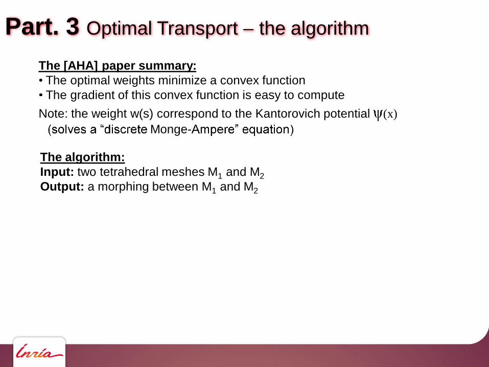
The [AHA] paper summary:
The optimal weights minimize a convex function
The gradient of this convex function is easy to compute
Note: the weight w(s) correspond to the Kantorovich potential (x)
Monge-
The algorithm:
Input: two tetrahedral meshes M1 and M2
Output: a morphing between M1 and M2

Part. 3 Optimal Transport the algorithm
The [AHA] paper summary:
The optimal weights minimize a convex function
The gradient of this convex function is easy to compute
Note: the weight w(s) correspond to the Kantorovich potential (x)
Monge-
The algorithm:
Input: two tetrahedral meshes M1 and M2
Output: a morphing between M1 and M2
Step 1: sample M2 with N points (s1 sN)
Step 2: initialize the weights (w1 wN) = (0 0)

Part. 3 Optimal Transport the algorithm
The [AHA] paper summary:
The optimal weights minimize a convex function
The gradient of this convex function is easy to compute
Note: the weight w(s) correspond to the Kantorovich potential (x)
Monge-
The algorithm:
Input: two tetrahedral meshes M1 and M2
Output: a morphing between M1 and M2
Step 1: sample M2 with N points (s1 sN)
Step 2: initialize the weights (w1 wN
Step 3: minimize g(w1 wN) with a quasi-Newton algorithm:
For each iterate (s1 sN)(k):

Part. 3 Optimal Transport the algorithm
The [AHA] paper summary:
The optimal weights minimize a convex function
The gradient of this convex function is easy to compute
Note: the weight w(s) correspond to the Kantorovich potential (x)
Monge-
The algorithm:
Input: two tetrahedral meshes M1 and M2
Output: a morphing between M1 and M2
Step 1: sample M2 with N points (s1 sN)
Step 2: initialize the weights (w1 wN) = (0 0)
Step 3: minimize g(w1 wN) with a quasi-Newton algorithm:
For each iterate (s1 sN)(k):
Compute Pow( (wi, si) M1 [Nivoliers, L 2014, Curves and Surfaces]

Part. 3 Optimal Transport the algorithm
Compute Pow( (wi, si) M1 [Nivoliers, L 2014, Curves and Surfaces]
Implementation in GEOGRAM (http://alice.loria.fr/software/geogram

Part. 3 Optimal Transport the algorithm
The [AHA] paper summary:
The optimal weights minimize a convex function
The gradient of this convex function is easy to compute
Note: the weight w(s) correspond to the Kantorovich potential (x)
Monge-
The algorithm:
Input: two tetrahedral meshes M1 and M2
Output: a morphing between M1 and M2
Step 1: sample M2 with N points (s1 sN)
Step 2: initialize the weights (w1 wN
Step 3: minimize g(w1 wN) with a quasi-Newton algorithm:
For each iterate (s1 sN)(k):
Compute Pow( (wi, si) M1 [L 2014, Curves and Surfaces]
Compute g and grad g
+ Multilevel version [Merigot 2011] (2D), [L 2014 arXiv, M2AN 2015] (3D)

Part. 3 Optimal Transport the algorithm
The [AHA] paper summary:
The optimal weights minimize a convex function
The gradient of this convex function is easy to compute
Note: the weight w(s) correspond to the Kantorovich potential (x)
Monge-
The algorithm:
Summary:
The algorithm computes the weights wi such that the power cells associated with
the Diracs correspond to the preimages of the Diracs.

Understanding Going
4

Part. 4 Optimal Transport ???
Wait a minute:
This means that one can move (and possibly deform)
a power diagram simply by changing the weights ?

Part. 4 Optimal Transport ???
Wait a minute:
This means that one can move (and possibly deform)
a power diagram simply by changing the weights ?
Reminder: Power diagram in 2d = intersection between
Voronoi diagram in 3d and IR2
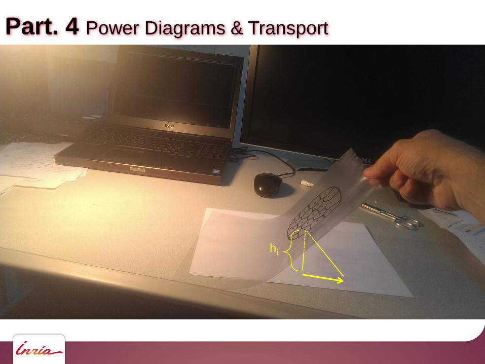
hi = sqrt(wmax wi)
Height of point i Weight of point i

Part. 4 Power Diagrams & Transport

Part. 4 Power Diagrams & Transport

Part. 4 Power Diagrams & Transport

Part. 4 Power Diagrams & Transport

Part. 4 Power Diagrams & Transport

Part. 4 Power Diagrams & Transport
Part. 4 Power Diagrams & Transport
hi

Part. 4 Power Diagrams & Transport

Part. 4 Power Diagrams & Transport

Part. 4 Power Diagrams & Transport

Part. 4 Power Diagrams & Transport

Part. 4 Optimal Transport still lost ? 2D examples
Numerical Experiment: Simple translation
Part. 4 Power Diagrams & Transport

Part. 4 Power Diagrams and Transport

Part. 4 Optimal Transport 2D examples
Numerical Experiment: Splitting a disk

Part. 4 Optimal Transport 2D examples
Numerical Experiment: A disk becomes two disks

Part. 4 Optimal Transport 3D examples
Numerical Experiment: A sphere becomes a cube

Part. 4 Optimal Transport 3D examples
Numerical Experiment: A sphere becomes two spheres

Part. 4 Optimal Transport 3D examples
Numerical Experiment: Armadillo to sphere

Part. 4 Optimal Transport 3D examples
Numerical Experiment: Other examples

Part. 4 Optimal Transport 3D examples
Numerical Experiment: Varying density

Part. 4 Optimal Transport 3D examples
Numerical Experiment: Performances

Part. 4 Optimal Transport 3D examples
Numerical Experiment: Performances
Note that a few years ago, several hours of supercomputer time were needed
for computing OT with a few thousand Dirac masses, with a combinatorial
algorithm in O(n3)

Part. 4 Optimal Transport 3D examples
Numerical Experiment: Performances
Note that a few years ago, several hours of supercomputer time were needed
for computing OT with a few thousand Dirac masses, with a combinatorial
algorithm in O(n3)
With the semi-discrete algorithm, it takes less than 10 seconds on my laptop

Part. 4 Optimal Transport 3D examples
Numerical Experiment: Performances
Note that a few years ago, several hours of supercomputer time were needed
for computing OT with a few thousand Dirac masses, with a combinatorial
algorithm in O(n3)
In the semi-discrete setting, my 3D version of multigrid algorithm
computes OT for 1 million Dirac masses in less than 1 hour on a laptop PC
Even much faster convergence can probably be reached with a true Newton
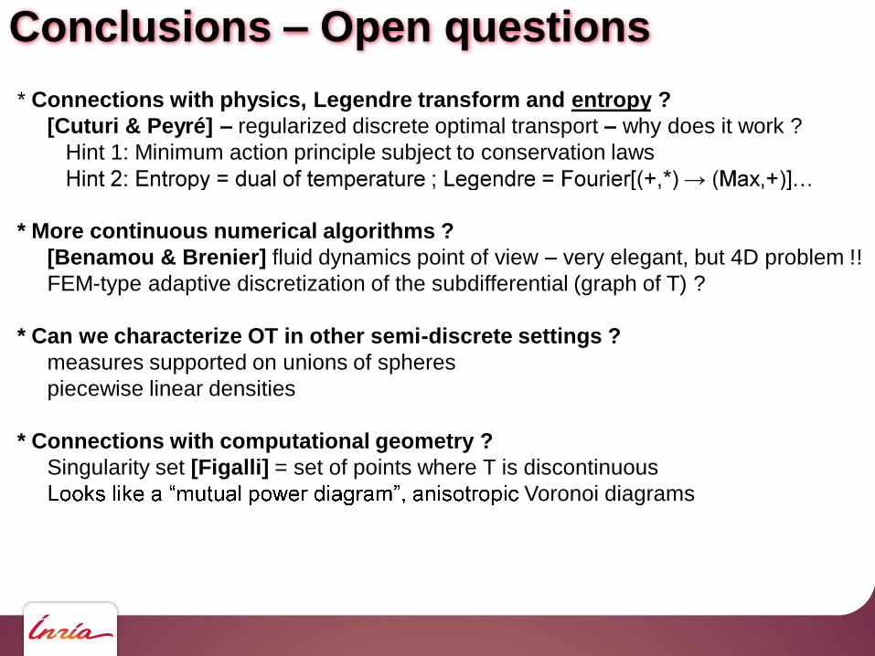
Conclusions Open questions
* Connections with physics, Legendre transform and entropy ?
[Cuturi & Peyré] regularized discrete optimal transport why does it work ?
Hint 1: Minimum action principle subject to conservation laws
* More continuous numerical algorithms ?
[Benamou & Brenier] fluid dynamics point of view very elegant, but 4D problem !!
FEM-type adaptive discretization of the subdifferential (graph of T) ?
* Can we characterize OT in other semi-discrete settings ?
measures supported on unions of spheres
piecewise linear densities
* Connections with computational geometry ?
Singularity set [Figalli] = set of points where T is discontinuous
Voronoi diagrams

Conclusions - ReferencesSome references (that this presentation is based on)
A Multiscale Approach to Optimal Transport,
Quentin Mérigot, Computer Graphics Forum, 2011
Variational Principles for Minkowski Type Problems, Discrete Optimal Transport,
and Discrete Monge-Ampere Equations
Xianfeng Gu, Feng Luo, Jian Sun, S.-T. Yau, ArXiv 2013
Minkowski-type theorems and least-squares clustering
AHA! (Aurenhammer, Hoffmann, and Aronov), SIAM J. on math. ana. 1998
Topics on Optimal Transportation, 2003
Optimal Transport Old and New, 2008
Cédric Villani
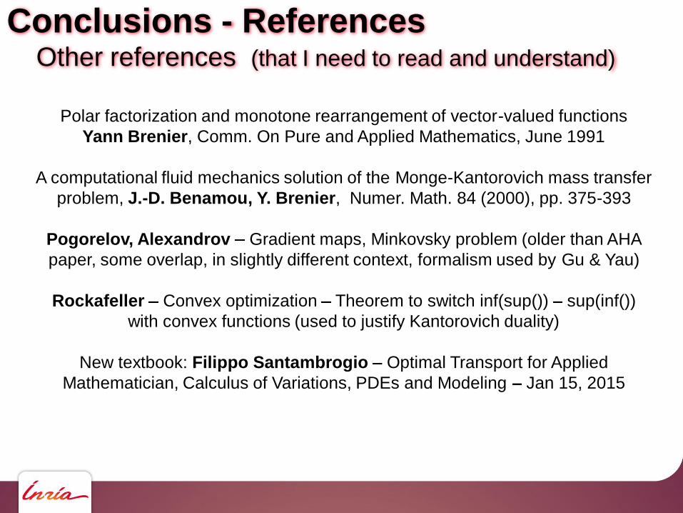
Conclusions - ReferencesOther references (that I need to read and understand)
Polar factorization and monotone rearrangement of vector-valued functions
Yann Brenier, Comm. On Pure and Applied Mathematics, June 1991
A computational fluid mechanics solution of the Monge-Kantorovich mass transfer
problem, J.-D. Benamou, Y. Brenier, Numer. Math. 84 (2000), pp. 375-393
Pogorelov, Alexandrov Gradient maps, Minkovsky problem (older than AHA
paper, some overlap, in slightly different context, formalism used by Gu & Yau)
Rockafeller Convex optimization Theorem to switch inf(sup()) sup(inf())
with convex functions (used to justify Kantorovich duality)
New textbook: Filippo Santambrogio Optimal Transport for Applied
Mathematician, Calculus of Variations, PDEs and Modeling Jan 15, 2015

Online resources
All the sourcecode/documentation available from:
alice.loria.fr/software/geogram
Computes semi-discrete OT in 3D
Scales up to millions Dirac masses on a laptop
L., A numerical algorithm for semi-discrete L2 OT in 3D,
ESAIM Math. Modeling and Analysis, accepted
(draft: http://arxiv.org/abs/1409.1279 <= to be fixed: bug
in MA equation in this version, fixed in M2AN journal version)

Acknowledgements
Funding: European Research Council french
GOODSHAPE ERC-StG-205693
VORPALINE ERC-PoC-334829
ANR MORPHO, ANR BECASIM
Quentin Merigot, Yann Brenier, Boris Thibert, Emmanuel Maitre,
Jean-David Benamou, Filippo Santambrogio, Edouard Oudet, Hervé Pajot.
ANR TOMMI, ANR GEOMETRYA


![OPTIMAL TRANSPORT IN GEOMETRY · Optimal transport is one such tool References • Topics in Optimal Transportation [TOT] (AMS, 2003): Introduction • Optimal transport, old and](https://img.pdfslide.net/doc/110x75/5ec621bb8d12144b8d424d3b/optimal-transport-in-geometry-optimal-transport-is-one-such-tool-references-a.jpg)