Embed Size (px)
Citation preview

Machine Learning for Everyone Else
Python 機械学習プログラミングデータ分析ライブラリー解説編
ver2.3 2017/01/12中井悦司 (Twitter @enakai00)
2
Python機械学習プログラミング
目次■ データ分析用のPythonライブラリー
■ NumPy & matplotlib入門
- 関数電卓として利用してみる
- NumPyによるベクトルと行列の計算
- 確率分布と乱数の取得
- グラフの描画
■ pandas入門
- pandasのデータフレーム
- データフレームからのデータ抽出
- その他のデータフレームの操作
■ サンプルコードの解説
- 最小二乗法のサンプルコード
- パーセプトロンのサンプルコード
■ 参考資料
3
Python機械学習プログラミング
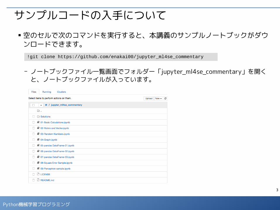
サンプルコードの入手について■ 空のセルで次のコマンドを実行すると、本講義のサンプルノートブックがダウ
ンロードできます。
- ノートブックファイル一覧画面でフォルダー「jupyter_ml4se_commentary」を開くと、ノートブックファイルが入っています。
!git clone https://github.com/enakai00/jupyter_ml4se_commentary
4
Python機械学習プログラミング
データ分析用のPythonライブラリー
5
Python機械学習プログラミング
NumPy, pandas, matplotlib について■ この資料では、主に下記のライブラリーを説明します。
- NumPy : ベクトルや行列の演算の他、主要な数学関数や乱数機能を提供します。
- pandas : Rに類似のデータフレーム(スプレッドシートのように、行/列に属性が付いたデータ構造)を提供します。
- matplotlib : グラフを描画します。
■ この資料の説明は、Jupyter Notebook上での実行を前提とします。
- はじめに下記のコマンドを実行して、必要なモジュールをインポートしてあるものとします。
import numpy as npimport matplotlib.pyplot as pltimport pandas as pdfrom pandas import Series, DataFrame
6
Python機械学習プログラミング
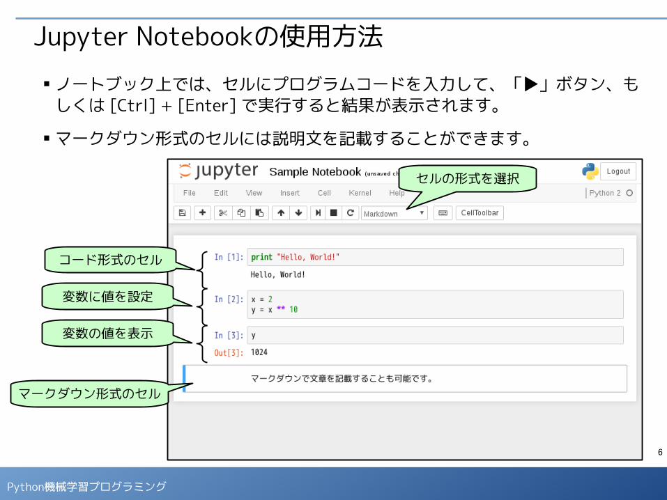
Jupyter Notebookの使用方法■ ノートブック上では、セルにプログラムコードを入力して、「▶」ボタン、も
しくは [Ctrl] + [Enter] で実行すると結果が表示されます。
■ マークダウン形式のセルには説明文を記載することができます。
セルの形式を選択
マークダウン形式のセル
コード形式のセル
変数に値を設定
変数の値を表示
7
Python機械学習プログラミング
NumPy & matplotlib入門
8
Python機械学習プログラミング
関数電卓として利用してみる
※ このパートでは、ノートブック「01-Basic Calculations.ipynb」を使用します。
9
Python機械学習プログラミング
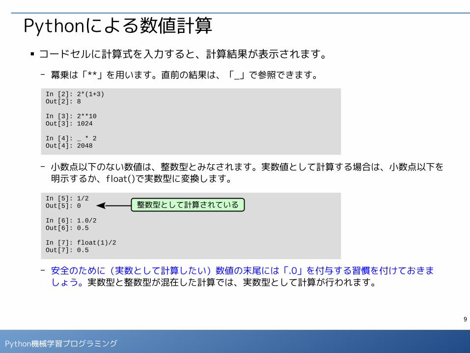
Pythonによる数値計算■ コードセルに計算式を入力すると、計算結果が表示されます。
- 冪乗は「**」を用います。直前の結果は、「_」で参照できます。
- 小数点以下のない数値は、整数型とみなされます。実数値として計算する場合は、小数点以下を明示するか、float()で実数型に変換します。
- 安全のために(実数として計算したい)数値の末尾には「.0」を付与する習慣を付けておきましょう。実数型と整数型が混在した計算では、実数型として計算が行われます。
In [2]: 2*(1+3)Out[2]: 8
In [3]: 2**10Out[3]: 1024
In [4]: _ * 2Out[4]: 2048
In [5]: 1/2Out[5]: 0
In [6]: 1.0/2Out[6]: 0.5
In [7]: float(1)/2Out[7]: 0.5
整数型として計算されている
10
Python機械学習プログラミング
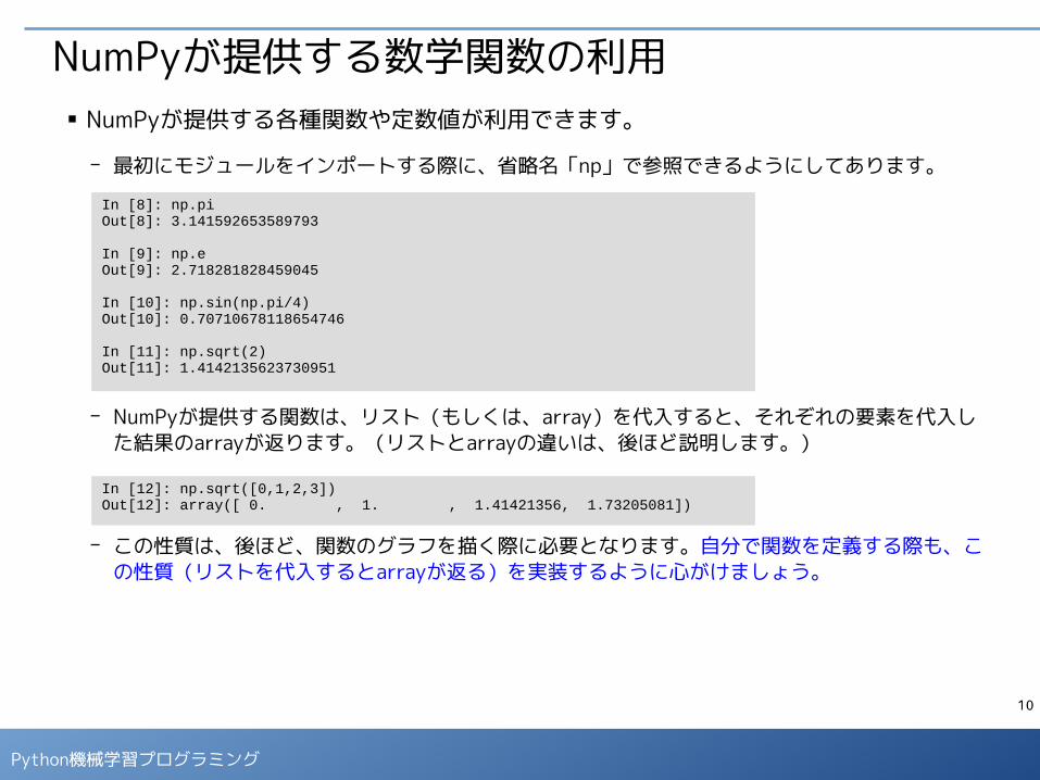
NumPyが提供する数学関数の利用■ NumPyが提供する各種関数や定数値が利用できます。
- 最初にモジュールをインポートする際に、省略名「np」で参照できるようにしてあります。
- NumPyが提供する関数は、リスト(もしくは、array)を代入すると、それぞれの要素を代入した結果のarrayが返ります。(リストとarrayの違いは、後ほど説明します。)
- この性質は、後ほど、関数のグラフを描く際に必要となります。自分で関数を定義する際も、この性質(リストを代入するとarrayが返る)を実装するように心がけましょう。
In [8]: np.piOut[8]: 3.141592653589793
In [9]: np.eOut[9]: 2.718281828459045
In [10]: np.sin(np.pi/4)Out[10]: 0.70710678118654746
In [11]: np.sqrt(2)Out[11]: 1.4142135623730951
In [12]: np.sqrt([0,1,2,3])Out[12]: array([ 0. , 1. , 1.41421356, 1.73205081])
11
Python機械学習プログラミング
散布図と折れ線グラフ
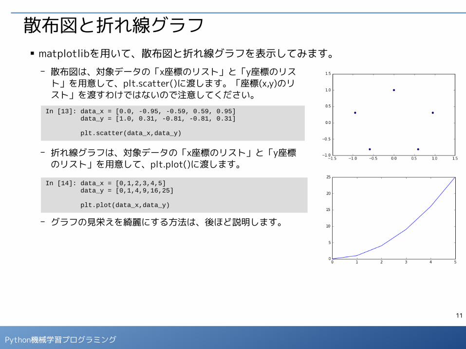
In [13]: data_x = [0.0, -0.95, -0.59, 0.59, 0.95] data_y = [1.0, 0.31, -0.81, -0.81, 0.31]
plt.scatter(data_x,data_y)
- 散布図は、対象データの「x座標のリスト」と「y座標のリスト」を用意して、plt.scatter()に渡します。「座標(x,y)のリスト」を渡すわけではないので注意してください。
- 折れ線グラフは、対象データの「x座標のリスト」と「y座標のリスト」を用意して、plt.plot()に渡します。
- グラフの見栄えを綺麗にする方法は、後ほど説明します。
In [14]: data_x = [0,1,2,3,4,5] data_y = [0,1,4,9,16,25]
plt.plot(data_x,data_y)
■ matplotlibを用いて、散布図と折れ線グラフを表示してみます。

12
Python機械学習プログラミング
散布図と折れ線グラフ- 関数のなめらかなグラフを描く際は、十分に細かく分割した「x座標のリスト」を用意して、対応する「y座標のリスト」を計算します。
- 「x座標のリスト」は、np.linspace()を使って生成すると便利です。「y座標のリスト」(data_y) の計算では、関数にリスト(array)を代入するとarrayが得られる性質を利用しています。
- np.linspace()の代わりに、np.arange()を使用することもできます。
In [15]: data_x = np.linspace(0,1,101) data_y = np.sin(2.0*np.pi*data_x)
plt.plot(data_x,data_y)
[0,1]を100分割した101個の実数を生成
data_x = np.arange(0,1.01,0.01)

13
Python機械学習プログラミング
練習問題■ ノートブック「01-Basic Calculations.ipynb」の末尾にある問題を解いてみましょう。
14
Python機械学習プログラミング
NumPyによるベクトルと行列の計算
※ このパートでは、ノートブック「02-Matrix and Vector.ipynb」を使用します。
15
Python機械学習プログラミング
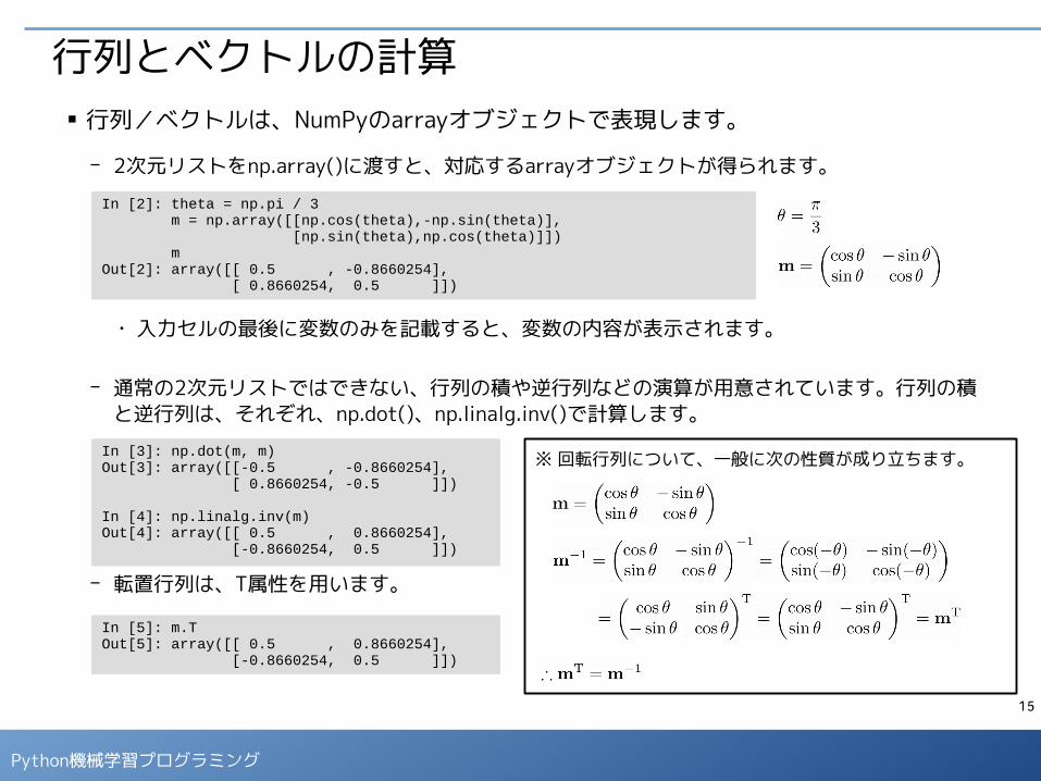
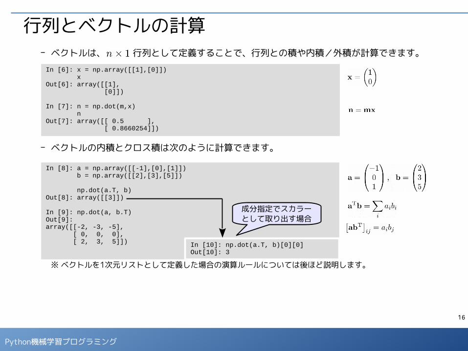
行列とベクトルの計算■ 行列/ベクトルは、NumPyのarrayオブジェクトで表現します。
- 2次元リストをnp.array()に渡すと、対応するarrayオブジェクトが得られます。
● 入力セルの最後に変数のみを記載すると、変数の内容が表示されます。
- 通常の2次元リストではできない、行列の積や逆行列などの演算が用意されています。行列の積と逆行列は、それぞれ、np.dot()、np.linalg.inv()で計算します。
- 転置行列は、T属性を用います。
In [2]: theta = np.pi / 3 m = np.array([[np.cos(theta),-np.sin(theta)], [np.sin(theta),np.cos(theta)]]) mOut[2]: array([[ 0.5 , -0.8660254], [ 0.8660254, 0.5 ]])
In [3]: np.dot(m, m)Out[3]: array([[-0.5 , -0.8660254], [ 0.8660254, -0.5 ]])
In [4]: np.linalg.inv(m)Out[4]: array([[ 0.5 , 0.8660254], [-0.8660254, 0.5 ]])
In [5]: m.TOut[5]: array([[ 0.5 , 0.8660254], [-0.8660254, 0.5 ]])
※ 回転行列について、一般に次の性質が成り立ちます。
16
Python機械学習プログラミング
行列とベクトルの計算- ベクトルは、 行列として定義することで、行列との積や内積/外積が計算できます。
- ベクトルの内積とクロス積は次のように計算できます。
※ ベクトルを1次元リストとして定義した場合の演算ルールについては後ほど説明します。
In [6]: x = np.array([[1],[0]]) xOut[6]: array([[1], [0]])
In [7]: n = np.dot(m,x) nOut[7]: array([[ 0.5 ], [ 0.8660254]])
In [8]: a = np.array([[-1],[0],[1]]) b = np.array([[2],[3],[5]])
np.dot(a.T, b)Out[8]: array([[3]])
In [9]: np.dot(a, b.T)Out[9]: array([[-2, -3, -5], [ 0, 0, 0], [ 2, 3, 5]]) In [10]: np.dot(a.T, b)[0][0]
Out[10]: 3
成分指定でスカラーとして取り出す場合
17
Python機械学習プログラミング
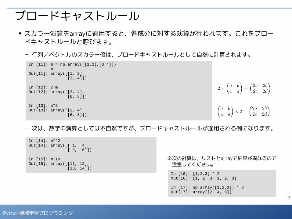
ブロードキャストルール■ スカラー演算をarrayに適用すると、各成分に対する演算が行われます。これをブロー
ドキャストルールと呼びます。
- 行列/ベクトルのスカラー倍は、ブロードキャストルールとして自然に計算されます。
- 次は、数学の演算としては不自然ですが、ブロードキャストルールが適用される例になります。
In [11]: m = np.array([[1,2],[3,4]]) mOut[11]: array([[1, 2], [3, 4]])
In [12]: 2*mOut[12]: array([[2, 4], [6, 8]])
In [13]: m*2Out[13]: array([[2, 4], [6, 8]])
In [14]: m**2Out[14]: array([[ 1, 4], [ 9, 16]])
In [15]: m+10Out[15]: array([[11, 12], [13, 14]])
In [16]: [1,2,3] * 2Out[16]: [1, 2, 3, 1, 2, 3]
In [17]: np.array([1,2,3]) * 2Out[17]: array([2, 4, 6])
※次の計算は、リストとarrayで結果が異なるので 注意してください。
18
Python機械学習プログラミング
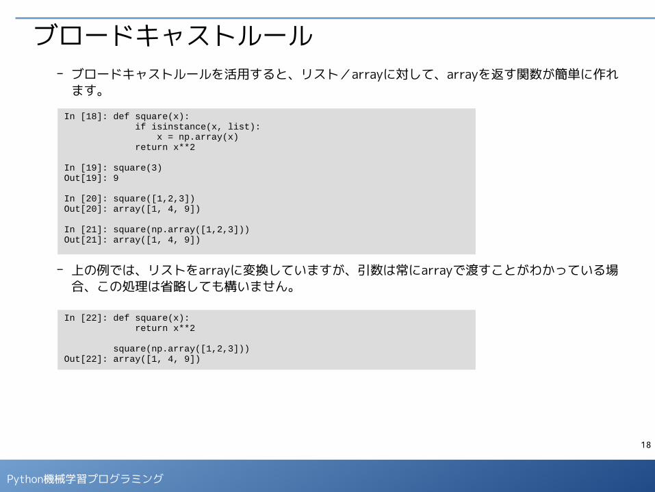
ブロードキャストルール- ブロードキャストルールを活用すると、リスト/arrayに対して、arrayを返す関数が簡単に作れ
ます。
- 上の例では、リストをarrayに変換していますが、引数は常にarrayで渡すことがわかっている場合、この処理は省略しても構いません。
In [18]: def square(x): if isinstance(x, list): x = np.array(x) return x**2
In [19]: square(3)Out[19]: 9
In [20]: square([1,2,3])Out[20]: array([1, 4, 9])
In [21]: square(np.array([1,2,3]))Out[21]: array([1, 4, 9])
In [22]: def square(x): return x**2
square(np.array([1,2,3]))Out[22]: array([1, 4, 9])

19
Python機械学習プログラミング
ブロードキャストルール■ 同じサイズのarray同士のスカラー演算は、対応する成分同士の演算になります。
- 行列の和/差は、自然に計算されます。
- 次のような演算も可能です。
※ サイズの異なるarray同士のスカラー演算にも、一定の法則でブロードキャストルールが適用されますが、 直感的にわかりにくい結果になるので、なるべく使用しない方がよいでしょう。
In [23]: a = np.array([[10,20],[30,40]]) aOut[23]: array([[10, 20], [30, 40]])
In [24]: b = np.array([[1,2],[3,4]]) bOut[24]: array([[1, 2], [3, 4]])
In [27]: a**bOut[27]: array([[ 10, 400], [ 27000, 2560000]])
In [25]: a+bOut[25]: array([[11, 22], [33, 44]])
In [26]: a-bOut[27]: array([[ 9, 18], [27, 36]])
20
Python機械学習プログラミング
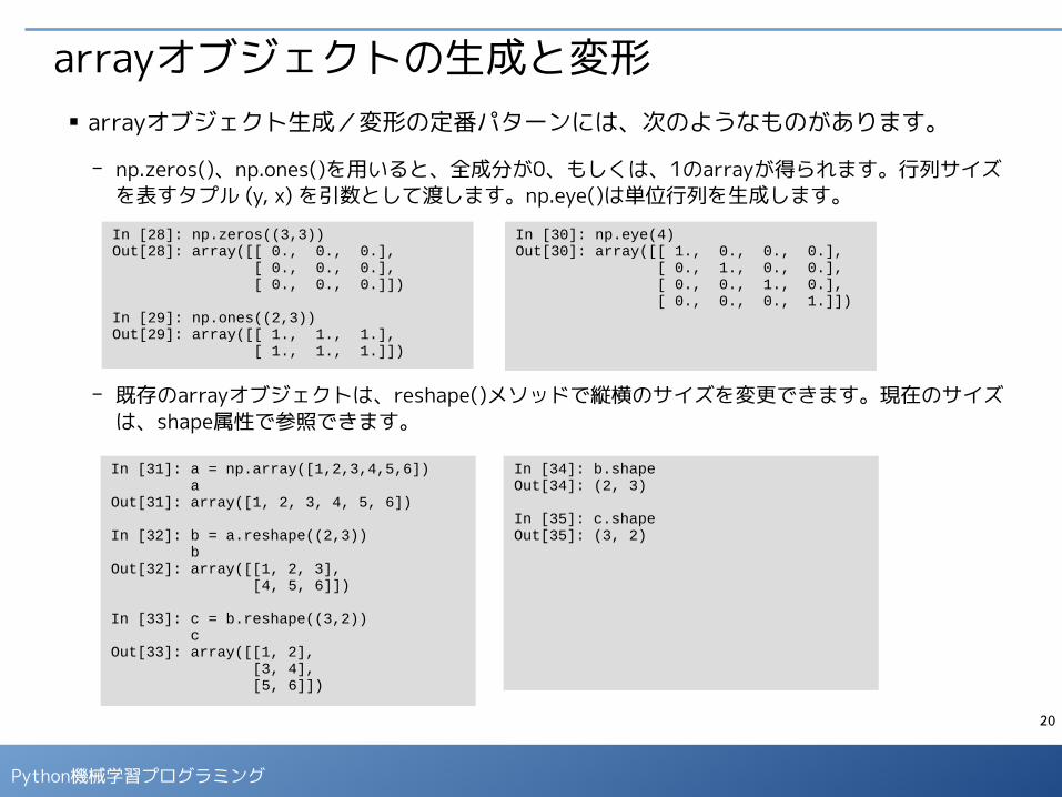
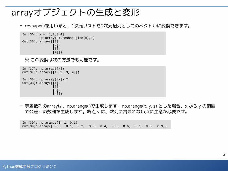
arrayオブジェクトの生成と変形■ arrayオブジェクト生成/変形の定番パターンには、次のようなものがあります。
- np.zeros()、np.ones()を用いると、全成分が0、もしくは、1のarrayが得られます。行列サイズを表すタプル (y, x) を引数として渡します。np.eye()は単位行列を生成します。
- 既存のarrayオブジェクトは、reshape()メソッドで縦横のサイズを変更できます。現在のサイズは、shape属性で参照できます。
In [28]: np.zeros((3,3))Out[28]: array([[ 0., 0., 0.], [ 0., 0., 0.], [ 0., 0., 0.]])
In [29]: np.ones((2,3))Out[29]: array([[ 1., 1., 1.], [ 1., 1., 1.]])
In [31]: a = np.array([1,2,3,4,5,6]) aOut[31]: array([1, 2, 3, 4, 5, 6])
In [32]: b = a.reshape((2,3)) bOut[32]: array([[1, 2, 3], [4, 5, 6]])
In [33]: c = b.reshape((3,2)) cOut[33]: array([[1, 2], [3, 4], [5, 6]])
In [34]: b.shapeOut[34]: (2, 3)
In [35]: c.shapeOut[35]: (3, 2)
In [30]: np.eye(4)Out[30]: array([[ 1., 0., 0., 0.], [ 0., 1., 0., 0.], [ 0., 0., 1., 0.], [ 0., 0., 0., 1.]])
21
Python機械学習プログラミング
arrayオブジェクトの生成と変形- reshape()を用いると、1次元リストを2次元配列としてのベクトルに変換できます。
※ この変換は次の方法でも可能です。
- 等差数列のarrayは、np.arange()で生成します。np.arange(x, y, s) とした場合、x から y の範囲で公差 s の数列を生成します。終点 y は、数列に含まれない点に注意が必要です。
In [36]: x = [1,2,3,4] np.array(x).reshape(len(x),1)Out[36]: array([[1], [2], [3], [4]])
In [39]: np.arange(0, 1, 0.1)Out[39]: array([ 0. , 0.1, 0.2, 0.3, 0.4, 0.5, 0.6, 0.7, 0.8, 0.9])
In [37]: np.array([x])Out[37]: array([[1, 2, 3, 4]])
In [38]: np.array([x]).TOut[38]: array([[1], [2], [3], [4]])
22
Python機械学習プログラミング
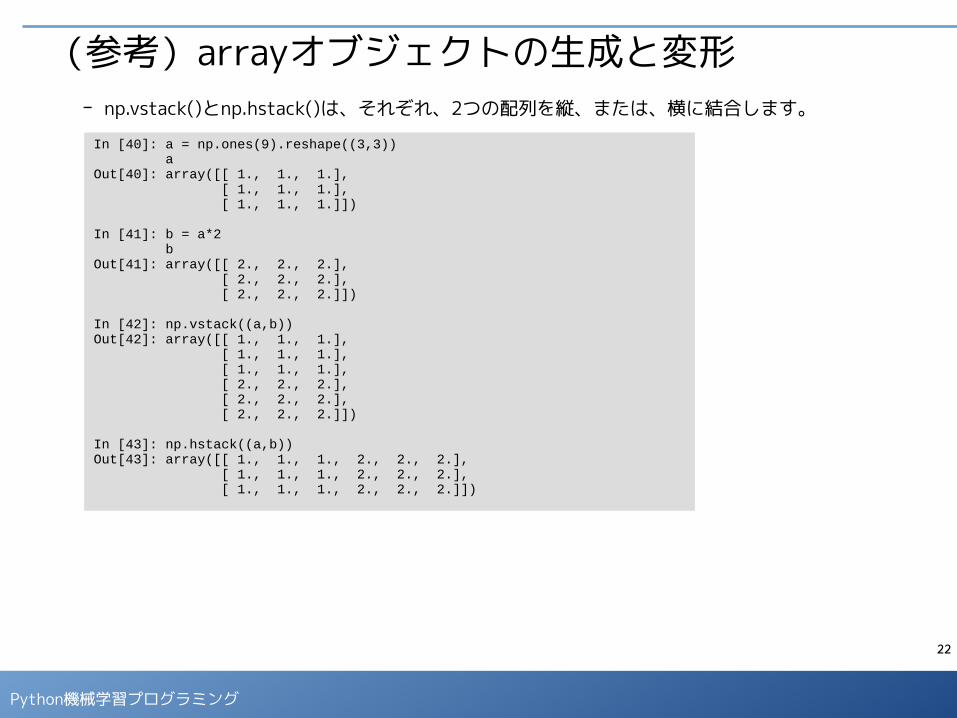
(参考)arrayオブジェクトの生成と変形- np.vstack()とnp.hstack()は、それぞれ、2つの配列を縦、または、横に結合します。
In [40]: a = np.ones(9).reshape((3,3)) aOut[40]: array([[ 1., 1., 1.], [ 1., 1., 1.], [ 1., 1., 1.]])
In [41]: b = a*2 bOut[41]: array([[ 2., 2., 2.], [ 2., 2., 2.], [ 2., 2., 2.]])
In [42]: np.vstack((a,b))Out[42]: array([[ 1., 1., 1.], [ 1., 1., 1.], [ 1., 1., 1.], [ 2., 2., 2.], [ 2., 2., 2.], [ 2., 2., 2.]])
In [43]: np.hstack((a,b))Out[43]: array([[ 1., 1., 1., 2., 2., 2.], [ 1., 1., 1., 2., 2., 2.], [ 1., 1., 1., 2., 2., 2.]])
23
Python機械学習プログラミング
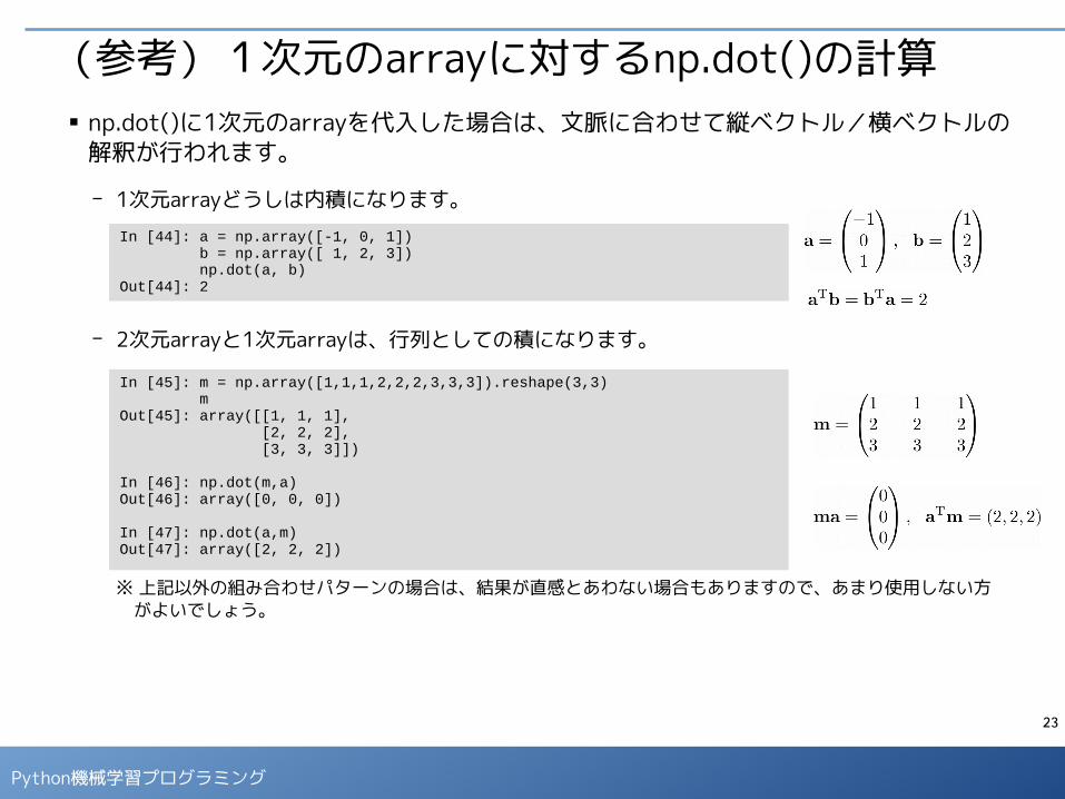
(参考)1次元のarrayに対するnp.dot()の計算■ np.dot()に1次元のarrayを代入した場合は、文脈に合わせて縦ベクトル/横ベクトルの
解釈が行われます。
- 1次元arrayどうしは内積になります。
- 2次元arrayと1次元arrayは、行列としての積になります。
※ 上記以外の組み合わせパターンの場合は、結果が直感とあわない場合もありますので、あまり使用しない方 がよいでしょう。
In [44]: a = np.array([-1, 0, 1]) b = np.array([ 1, 2, 3]) np.dot(a, b)Out[44]: 2
In [45]: m = np.array([1,1,1,2,2,2,3,3,3]).reshape(3,3) mOut[45]: array([[1, 1, 1], [2, 2, 2], [3, 3, 3]])
In [46]: np.dot(m,a)Out[46]: array([0, 0, 0])
In [47]: np.dot(a,m)Out[47]: array([2, 2, 2])
24
Python機械学習プログラミング
練習問題■ ノートブック「02-Matrix and Vector.ipynb」の末尾にある問題を解いてみましょう。
25
Python機械学習プログラミング
確率分布と乱数の取得
※ このパートでは、ノートブック「03-Random Numbers.ipynb」を使用します。
26
Python機械学習プログラミング
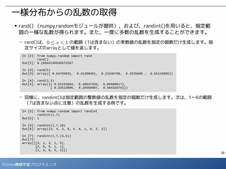
一様分布からの乱数の取得■ rand() (numpy.randomモジュールが提供)、および、randint()を用いると、指定範囲の一様な乱数が得られます。また、一度に多数の乱数を生成することができます。
- rand()は、 の範囲(1は含まない)の実数値の乱数を指定の個数だけ生成します。指定サイズのarrayとして値を返します。
- 同様に、randint()は指定範囲の整数値の乱数を指定の個数だけ生成します。次は、1〜6の範囲(7は含まない点に注意)の乱数を生成する例です。
In [2]: from numpy.random import rand rand()Out[2]: 0.19644145945572267
In [3]: rand(5)Out[3]: array([ 0.64765831, 0.41288461, 0.21530768, 0.3225688 , 0.55119995])
In [4]: rand(2,3)Out[4]: array([[ 0.63193604, 0.48647432, 0.06980617], [ 0.32513886, 0.29350987, 0.58432974]])
In [5]: from numpy.random import randint randint(1,7)Out[5]: 1
In [6]: randint(1,7,10)Out[6]: array([2, 4, 3, 6, 4, 6, 1, 6, 2, 3])
In [7]: randint(1,7,(3,5))Out[7]: array([[3, 1, 3, 1, 5], [2, 5, 5, 1, 1], [1, 3, 6, 5, 2]])

27
Python機械学習プログラミング
正規分布からの乱数の取得■ numpy.randomモジュールの normal() を用いると、正規分布からの乱数が得られます。
- 次のように、loc(平均)、scale(標準偏差)、size(arrayのサイズ)を指定します。最後の例のように、パラメータ名を省略しても構いません。
- 1000個の乱数を発生して、ヒストグラムを表示します。
In [8]: from numpy.random import normal normal(loc=0,scale=3,size=10)Out[8]: array([-0.45405421, 1.03407066, -6.06638636, -1.47014096, 2.4127684 , -0.60084586, -2.20008908, -2.49174201, -5.53419474, -2.99053036])
In [9]: normal(loc=0,scale=3,size=(3,2))Out[9]: array([[ 4.94332685, -2.65134418], [-5.97073959, -0.94864428], [-1.04192588, 2.29266043]])
In [10]: normal(0,3,(3,2))Out[10]: array([[ 4.55288412, -3.28343893], [ 2.981074 , -2.05497678], [ 0.08205987, 0.77338863]])
In [5]: val = normal(10,3,size=1000)
In [6]: plt.hist(val, bins=20)
28
Python機械学習プログラミング
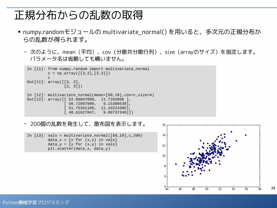
正規分布からの乱数の取得■ numpy.randomモジュールの multivariate_normal() を用いると、多次元の正規分布か
らの乱数が得られます。
- 次のように、mean(平均)、cov(分散共分散行列)、size(arrayのサイズ)を指定します。パラメータ名は省略しても構いません。
- 200個の乱数を発生して、散布図を表示します。
In [11]: from numpy.random import multivariate_normal c = np.array([[3,2],[2,3]]) cOut[11]: array([[3, 2], [2, 3]])
In [12]: multivariate_normal(mean=[50,10],cov=c,size=4)Out[12]: array([[ 52.09847888, 11.7263966 ], [ 50.72997909, 9.15308538], [ 51.75341106, 11.19224385], [ 48.61627847, 9.09737349]])
In [13]: vals = multivariate_normal([50,10],c,200) data_x = [x for (x,y) in vals] data_y = [y for (x,y) in vals] plt.scatter(data_x, data_y)
29
Python機械学習プログラミング
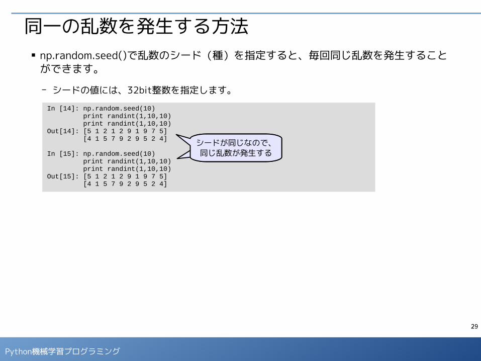
同一の乱数を発生する方法■ np.random.seed()で乱数のシード(種)を指定すると、毎回同じ乱数を発生すること
ができます。
- シードの値には、32bit整数を指定します。
In [14]: np.random.seed(10) print randint(1,10,10) print randint(1,10,10)Out[14]: [5 1 2 1 2 9 1 9 7 5] [4 1 5 7 9 2 9 5 2 4]
In [15]: np.random.seed(10) print randint(1,10,10) print randint(1,10,10)Out[15]: [5 1 2 1 2 9 1 9 7 5] [4 1 5 7 9 2 9 5 2 4]
シードが同じなので、同じ乱数が発生する
シードが同じなので、同じ乱数が発生する

30
Python機械学習プログラミング
練習問題■ ノートブック「03-Random Numbers.ipynb」の末尾にある問題を解いてみましょう。

31
Python機械学習プログラミング
グラフの描画
※ このパートでは、ノートブック「04-Graph.ipynb」を使用します。
32
Python機械学習プログラミング
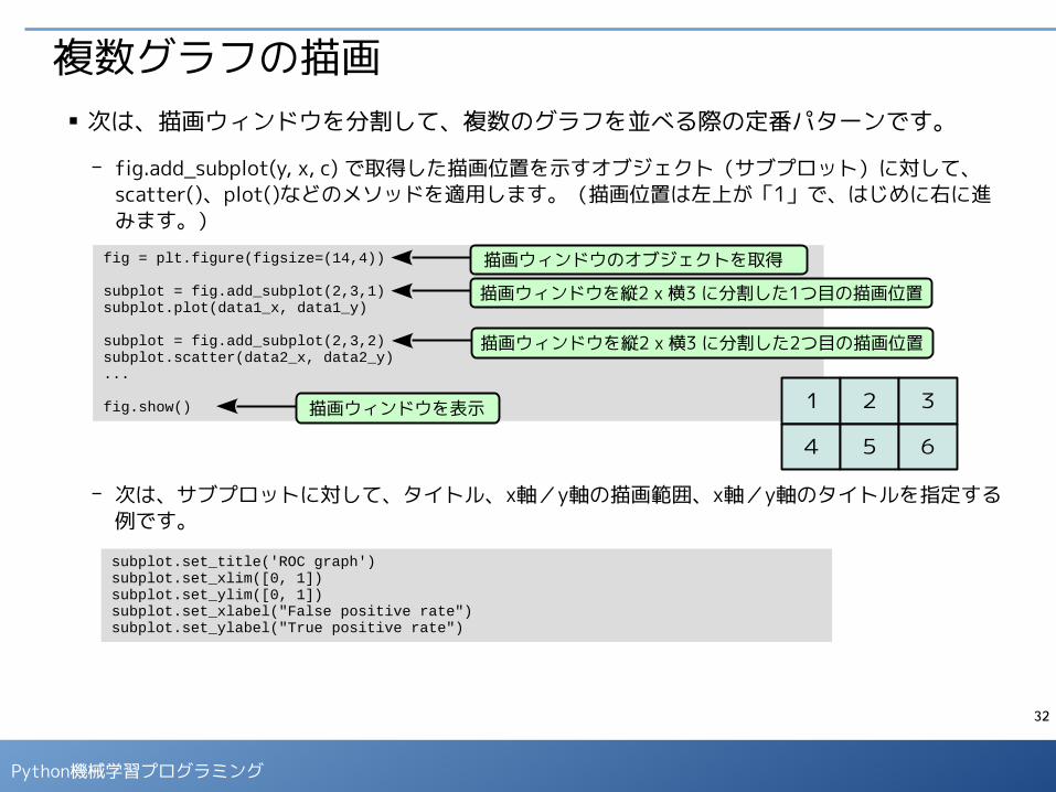
複数グラフの描画■ 次は、描画ウィンドウを分割して、複数のグラフを並べる際の定番パターンです。
- fig.add_subplot(y, x, c) で取得した描画位置を示すオブジェクト(サブプロット)に対して、scatter()、plot()などのメソッドを適用します。(描画位置は左上が「1」で、はじめに右に進みます。)
- 次は、サブプロットに対して、タイトル、x軸/y軸の描画範囲、x軸/y軸のタイトルを指定する例です。
fig = plt.figure(figsize=(14,4))
subplot = fig.add_subplot(2,3,1)subplot.plot(data1_x, data1_y)
subplot = fig.add_subplot(2,3,2)subplot.scatter(data2_x, data2_y)...
fig.show()
描画ウィンドウのオブジェクトを取得
描画ウィンドウを縦2 x 横3 に分割した1つ目の描画位置
描画ウィンドウを縦2 x 横3 に分割した2つ目の描画位置
1
4
2
5
3
6
描画ウィンドウを表示
subplot.set_title('ROC graph')subplot.set_xlim([0, 1])subplot.set_ylim([0, 1])subplot.set_xlabel("False positive rate")subplot.set_ylabel("True positive rate")
33
Python機械学習プログラミング
サイコロのシュミレーションをグラフ表示
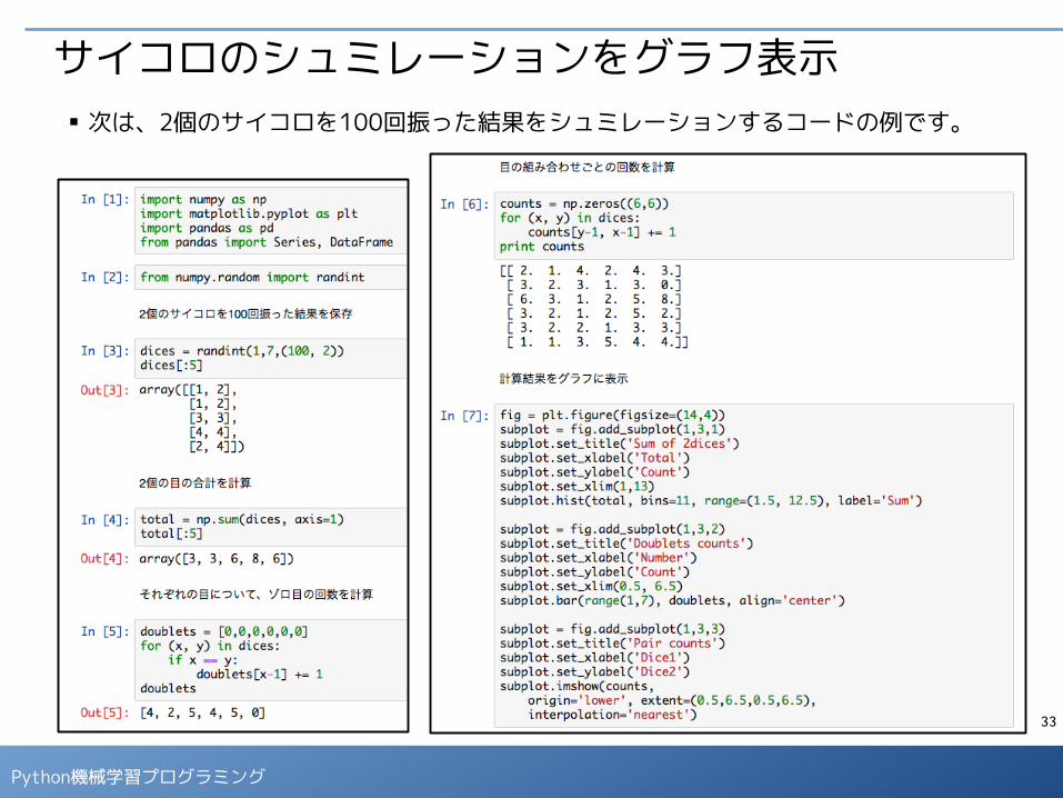
■ 次は、2個のサイコロを100回振った結果をシュミレーションするコードの例です。
■ 次は、2個のサイコロを100回振った結果をシュミレーションするコードの例です。

34
Python機械学習プログラミング
「ヒートマップ」と呼ばれるグラフで値が大きいほど「熱い色」になります
■ 前ページのコードを実行すると以下の統計値がグラフ表示されます。
- 2個の目の合計ごとの出現回数
- それぞれの目についてゾロ目が出た回数
- 目の組み合わせごとの回数の比較
サイコロのシュミレーションをグラフ表示
35
Python機械学習プログラミング
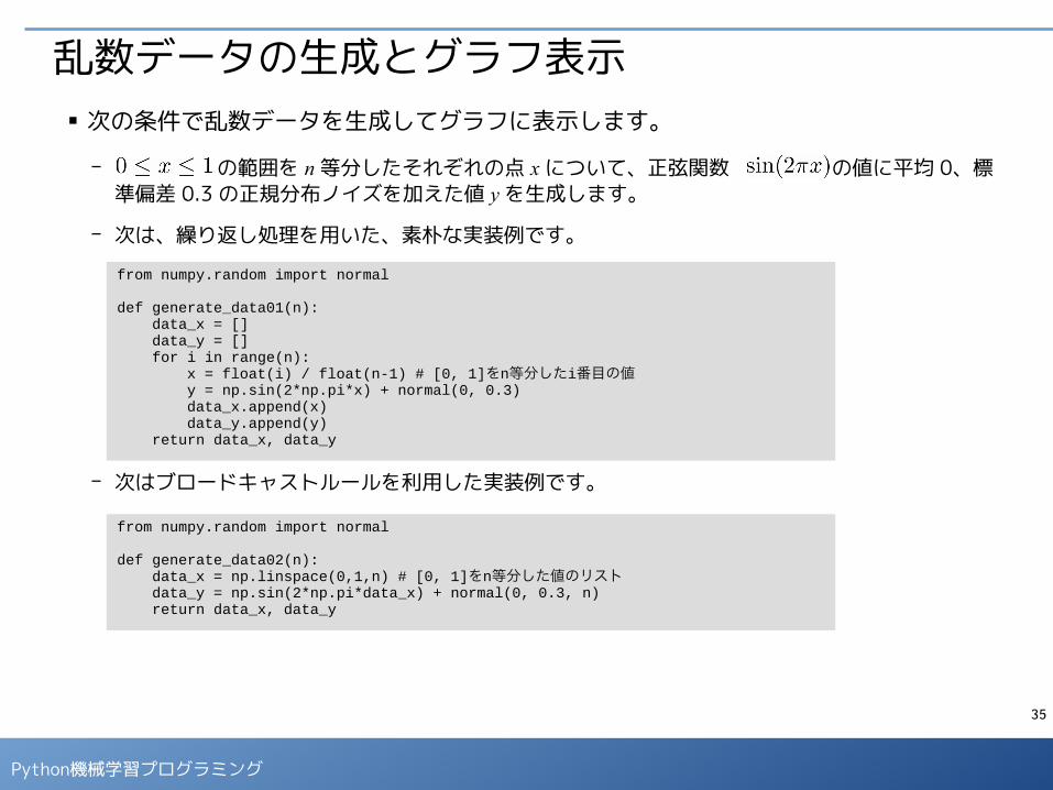
乱数データの生成とグラフ表示■ 次の条件で乱数データを生成してグラフに表示します。
- の範囲を n 等分したそれぞれの点 x について、正弦関数 の値に平均 0、標準偏差 0.3 の正規分布ノイズを加えた値 y を生成します。
- 次は、繰り返し処理を用いた、素朴な実装例です。
- 次はブロードキャストルールを利用した実装例です。
from numpy.random import normal
def generate_data01(n): data_x = [] data_y = [] for i in range(n): x = float(i) / float(n-1) # [0, 1]をn等分したi番目の値 y = np.sin(2*np.pi*x) + normal(0, 0.3) data_x.append(x) data_y.append(y) return data_x, data_y
from numpy.random import normal
def generate_data02(n): data_x = np.linspace(0,1,n) # [0, 1]をn等分した値のリスト data_y = np.sin(2*np.pi*data_x) + normal(0, 0.3, n) return data_x, data_y
36
Python機械学習プログラミング
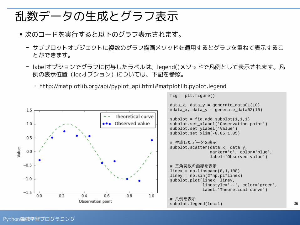
乱数データの生成とグラフ表示■ 次のコードを実行すると以下のグラフ表示されます。
- サブプロットオブジェクトに複数のグラフ描画メソッドを適用するとグラフを重ねて表示することができます。
- labelオプションでグラフに付与したラベルは、legend()メソッドで凡例として表示されます。凡例の表示位置(locオプション)については、下記を参照。
● http://matplotlib.org/api/pyplot_api.html#matplotlib.pyplot.legendfig = plt.figure()
data_x, data_y = generate_data01(10)#data_x, data_y = generate_data02(10)
subplot = fig.add_subplot(1,1,1)subplot.set_xlabel('Observation point')subplot.set_ylabel('Value')subplot.set_xlim(-0.05,1.05)
# 生成したデータを表示subplot.scatter(data_x, data_y, marker='o', color='blue', label='Observed value')
# 三角関数の曲線を表示linex = np.linspace(0,1,100)liney = np.sin(2*np.pi*linex)subplot.plot(linex, liney, linestyle='--', color='green', label='Theoretical curve')
# 凡例を表示subplot.legend(loc=1)
37
Python機械学習プログラミング
練習問題■ ノートブック「04-Graph.ipynb」の末尾にある問題を解いてみ
ましょう。
38
Python機械学習プログラミング
pandas入門
39
Python機械学習プログラミング
pandasのデータフレーム
※ このパートでは、ノートブック「05-pandas DataFrame-01.ipynb」を使用します。
40
Python機械学習プログラミング
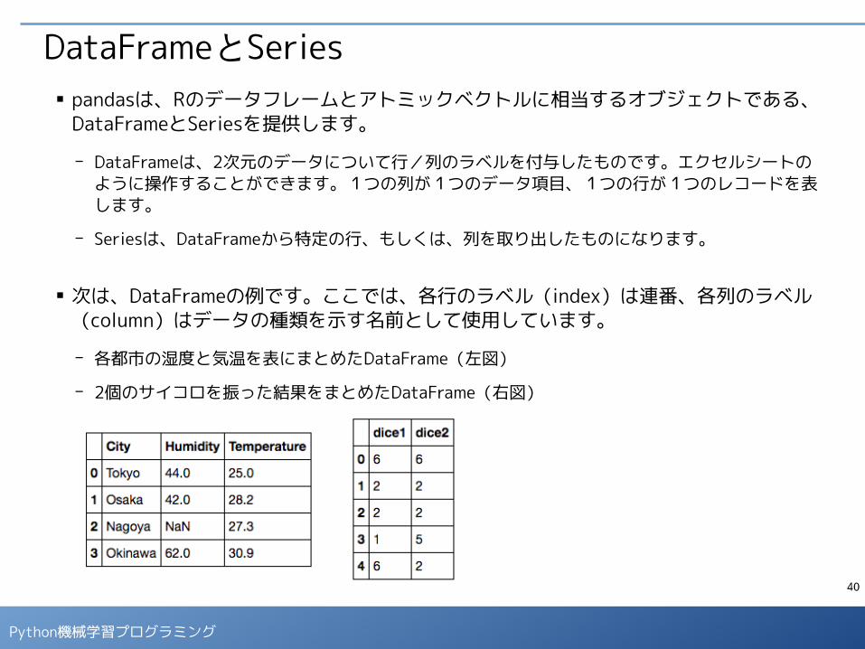
DataFrameとSeries■ pandasは、Rのデータフレームとアトミックベクトルに相当するオブジェクトである、DataFrameとSeriesを提供します。
- DataFrameは、2次元のデータについて行/列のラベルを付与したものです。エクセルシートのように操作することができます。1つの列が1つのデータ項目、1つの行が1つのレコードを表します。
- Seriesは、DataFrameから特定の行、もしくは、列を取り出したものになります。
■ 次は、DataFrameの例です。ここでは、各行のラベル(index)は連番、各列のラベル(column)はデータの種類を示す名前として使用しています。
- 各都市の湿度と気温を表にまとめたDataFrame(左図)
- 2個のサイコロを振った結果をまとめたDataFrame(右図)
41
Python機械学習プログラミング
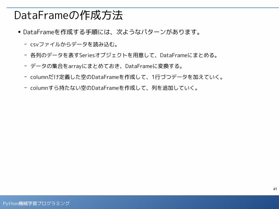
DataFrameの作成方法■ DataFrameを作成する手順には、次ようなパターンがあります。
- csvファイルからデータを読み込む。
- 各列のデータを表すSeriesオブジェクトを用意して、DataFrameにまとめる。
- データの集合をarrayにまとめておき、DataFrameに変換する。
- columnだけ定義した空のDataFrameを作成して、1行づつデータを加えていく。
- columnすら持たない空のDataFrameを作成して、列を追加していく。
42
Python機械学習プログラミング
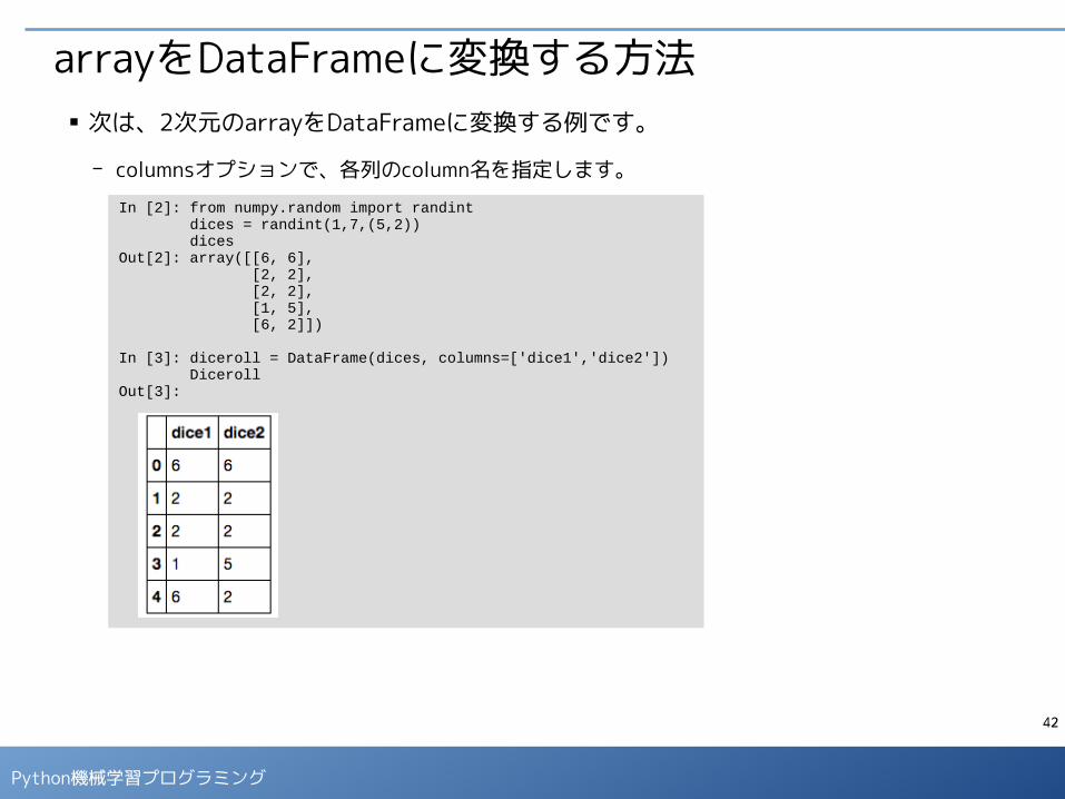
arrayをDataFrameに変換する方法■ 次は、2次元のarrayをDataFrameに変換する例です。
- columnsオプションで、各列のcolumn名を指定します。
In [2]: from numpy.random import randint dices = randint(1,7,(5,2)) dicesOut[2]: array([[6, 6], [2, 2], [2, 2], [1, 5], [6, 2]])
In [3]: diceroll = DataFrame(dices, columns=['dice1','dice2']) DicerollOut[3]:
43
Python機械学習プログラミング
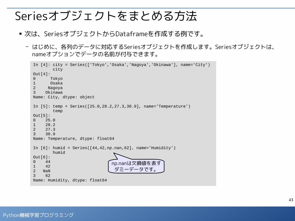
Seriesオブジェクトをまとめる方法■ 次は、SeriesオブジェクトからDataframeを作成する例です。
- はじめに、各列のデータに対応するSeriesオブジェクトを作成します。Seriesオブジェクトは、nameオプションでデータの名前が付与できます。
In [4]: city = Series(['Tokyo','Osaka','Nagoya','Okinawa'], name='City') cityOut[4]: 0 Tokyo1 Osaka2 Nagoya3 OkinawaName: City, dtype: object
In [5]: temp = Series([25.0,28.2,27.3,30.9], name='Temperature') tempOut[5]: 0 25.01 28.22 27.33 30.9Name: Temperature, dtype: float64
In [6]: humid = Series([44,42,np.nan,62], name='Humidity') humidOut[6]: 0 441 422 NaN3 62Name: Humidity, dtype: float64
np.nanは欠損値を表すダミーデータです。

44
Python機械学習プログラミング
Seriesオブジェクトをまとめる方法- 各列のcolumn名と対応するSeriesオブジェクトのディクショナリを与えて、DataFrameを生成し
ます。
- Seriesオブジェクトの代わりに、リストを用いてもDataFrameを生成することができます。
In [7]: cities = DataFrame({'City':city, 'Temperature':temp, 'Humidity':humid}) citiesOut[7]:
In [8]: data = {'City': ['Tokyo','Osaka','Nagoya','Okinawa'], 'Temperature': [25.0,28.2,27.3,30.9], 'Humidity': [44,42,np.nan,62]} cities = DataFrame(data)Out[8]:
45
Python機械学習プログラミング
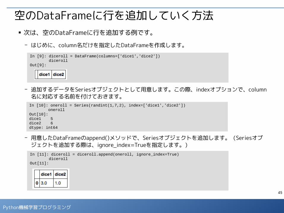
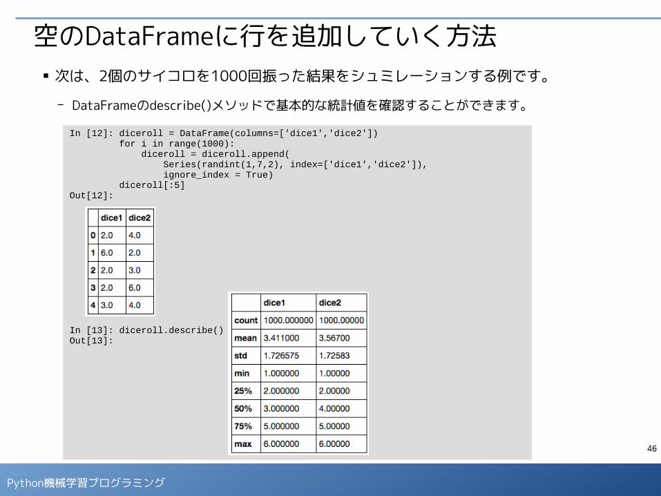
空のDataFrameに行を追加していく方法■ 次は、空のDataFrameに行を追加する例です。
- はじめに、column名だけを指定したDataFrameを作成します。
- 追加するデータをSeriesオブジェクトとして用意します。この際、indexオプションで、column名に対応する名前を付けておきます。
- 用意したDataFrameのappend()メソッドで、Seriesオブジェクトを追加します。(Seriesオブジェクトを追加する際は、ignore_index=Trueを指定します。)
In [9]: diceroll = DataFrame(columns=['dice1','dice2']) dicerollOut[9]:
In [10]: oneroll = Series(randint(1,7,2), index=['dice1','dice2']) onerollOut[10]: dice1 5dice2 6dtype: int64
In [11]: diceroll = diceroll.append(oneroll, ignore_index=True) dicerollOut[11]:
46
Python機械学習プログラミング
空のDataFrameに行を追加していく方法■ 次は、2個のサイコロを1000回振った結果をシュミレーションする例です。
- DataFrameのdescribe()メソッドで基本的な統計値を確認することができます。
In [12]: diceroll = DataFrame(columns=['dice1','dice2']) for i in range(1000): diceroll = diceroll.append( Series(randint(1,7,2), index=['dice1','dice2']), ignore_index = True) diceroll[:5]Out[12]:
In [13]: diceroll.describe()Out[13]:
47
Python機械学習プログラミング
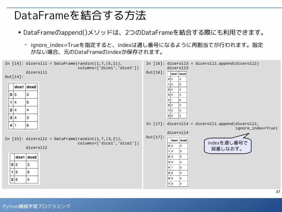
DataFrameを結合する方法■ DataFrameのappend()メソッドは、2つのDataFrameを結合する際にも利用できます。
- ignore_index=Trueを指定すると、indexは通し番号になるように再割当てが行われます。指定がない場合、元のDataFrameのindexが保存されます。
In [16]: diceroll3 = diceroll1.append(diceroll2) diceroll3Out[16]:
In [17]: diceroll4 = diceroll1.append(diceroll2, ignore_index=True) diceroll4Out[17]:
In [14]: diceroll1 = DataFrame(randint(1,7,(5,2)), columns=['dice1','dice2']) diceroll1Out[14]:
In [15]: diceroll2 = DataFrame(randint(1,7,(3,2)), columns=['dice1','dice2']) diceroll2
indexを通し番号で採番しなおす。
48
Python機械学習プログラミング
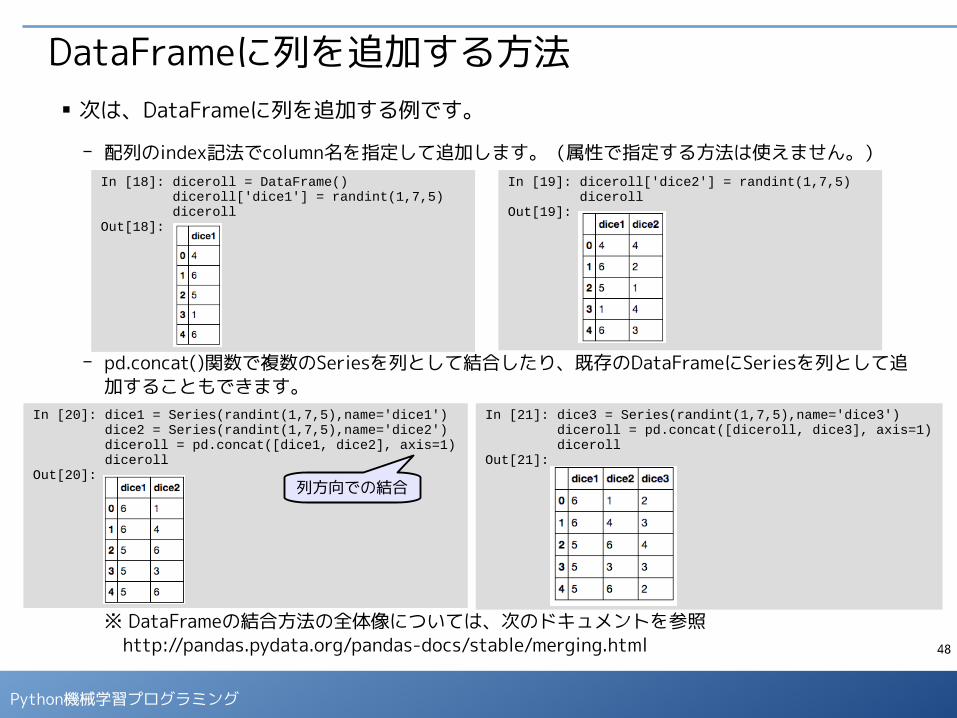
DataFrameに列を追加する方法■ 次は、DataFrameに列を追加する例です。
- 配列のindex記法でcolumn名を指定して追加します。(属性で指定する方法は使えません。)
- pd.concat()関数で複数のSeriesを列として結合したり、既存のDataFrameにSeriesを列として追加することもできます。
※ DataFrameの結合方法の全体像については、次のドキュメントを参照 http://pandas.pydata.org/pandas-docs/stable/merging.html
In [18]: diceroll = DataFrame() diceroll['dice1'] = randint(1,7,5) dicerollOut[18]:
In [19]: diceroll['dice2'] = randint(1,7,5) dicerollOut[19]:
In [20]: dice1 = Series(randint(1,7,5),name='dice1') dice2 = Series(randint(1,7,5),name='dice2') diceroll = pd.concat([dice1, dice2], axis=1) dicerollOut[20]:
In [21]: dice3 = Series(randint(1,7,5),name='dice3') diceroll = pd.concat([diceroll, dice3], axis=1) dicerollOut[21]:
列方向での結合
49
Python機械学習プログラミング
練習問題■ ノートブック「05-pandas DataFrame-01.ipynb」の末尾にあ
る問題を解いてみましょう。
50
Python機械学習プログラミング
データフレームからのデータ抽出
※ このパートでは、ノートブック「06-pandas DataFrame-02.ipynb」を使用します。
51
Python機械学習プログラミング
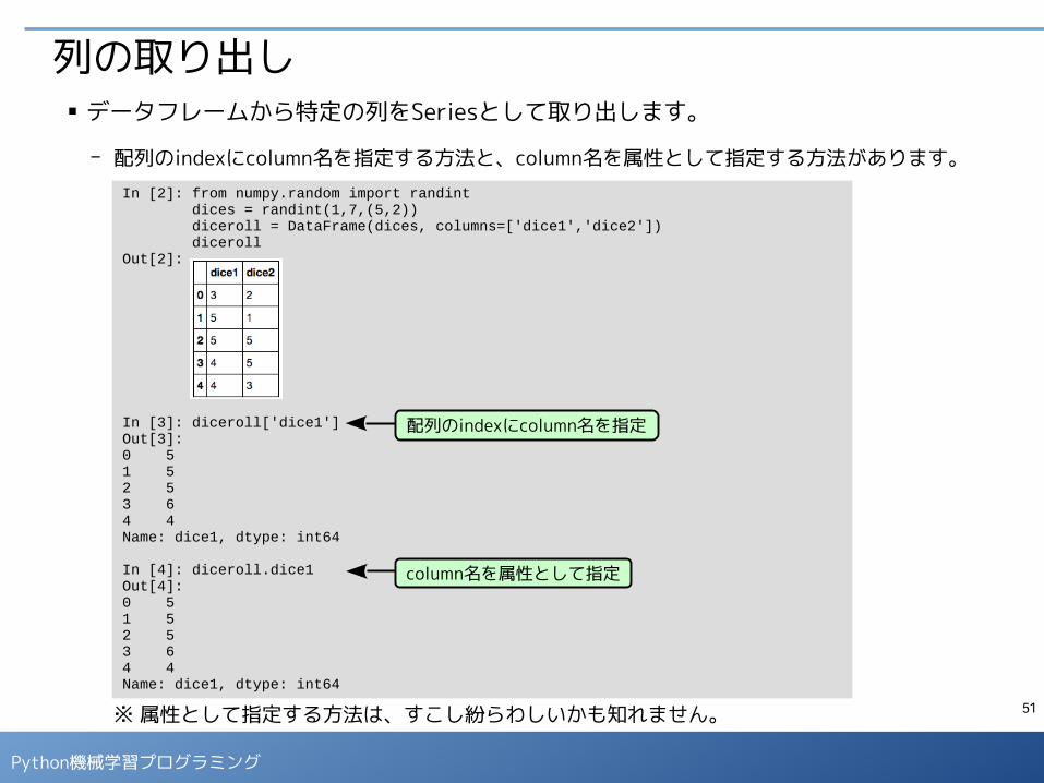
列の取り出し■ データフレームから特定の列をSeriesとして取り出します。
- 配列のindexにcolumn名を指定する方法と、column名を属性として指定する方法があります。
※ 属性として指定する方法は、すこし紛らわしいかも知れません。
In [2]: from numpy.random import randint dices = randint(1,7,(5,2)) diceroll = DataFrame(dices, columns=['dice1','dice2']) dicerollOut[2]:
In [3]: diceroll['dice1']Out[3]: 0 51 52 53 64 4Name: dice1, dtype: int64
In [4]: diceroll.dice1Out[4]: 0 51 52 53 64 4Name: dice1, dtype: int64
配列のindexにcolumn名を指定
column名を属性として指定
52
Python機械学習プログラミング
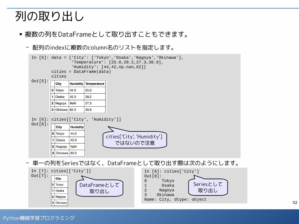
列の取り出し■ 複数の列をDataFrameとして取り出すこともできます。
- 配列のindexに複数のcolumn名のリストを指定します。
- 単一の列をSeriesではなく、DataFrameとして取り出す際は次のようにします。
In [5]: data = {'City': ['Tokyo','Osaka','Nagoya','Okinawa'], 'Temperature': [25.0,28.2,27.3,30.9], 'Humidity': [44,42,np.nan,62]} cities = DataFrame(data) citiesOut[5]:
In [6]: cities[['City', 'Humidity']]Out[6]:
cities['City', 'Humidity'] ではないので注意
In [7]: cities[['City']]Out[7]:
In [8]: cities['City']Out[8]: 0 Tokyo1 Osaka2 Nagoya3 OkinawaName: City, dtype: object
DataFrameとして取り出し
Seriesとして取り出し
53
Python機械学習プログラミング
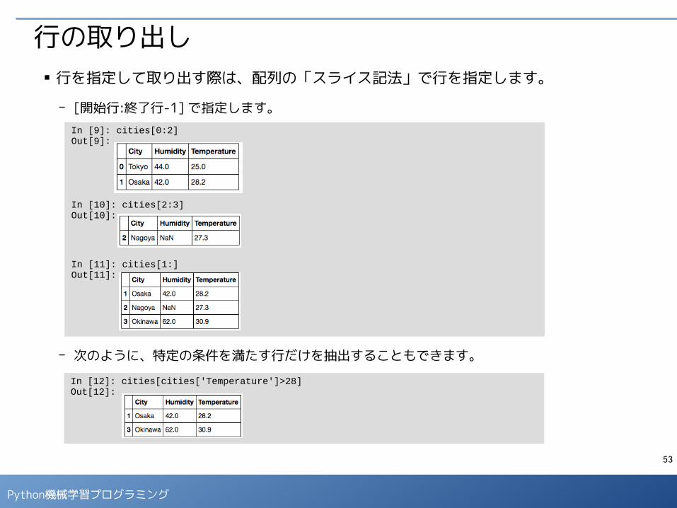
行の取り出し■ 行を指定して取り出す際は、配列の「スライス記法」で行を指定します。
- [開始行:終了行-1] で指定します。
- 次のように、特定の条件を満たす行だけを抽出することもできます。
In [9]: cities[0:2]Out[9]:
In [10]: cities[2:3]Out[10]:
In [11]: cities[1:]Out[11]:
In [12]: cities[cities['Temperature']>28]Out[12]:
54
Python機械学習プログラミング
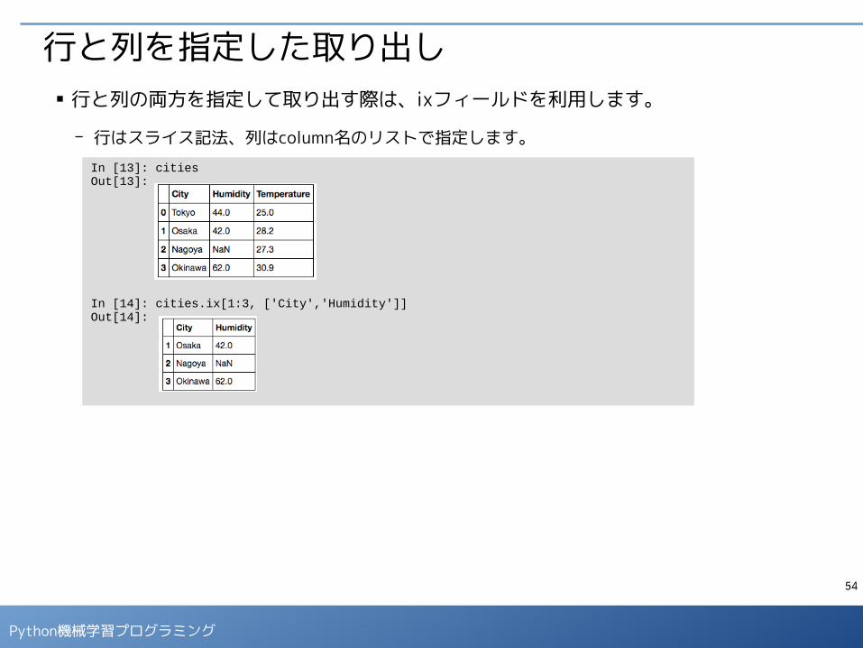
行と列を指定した取り出し■ 行と列の両方を指定して取り出す際は、ixフィールドを利用します。
- 行はスライス記法、列はcolumn名のリストで指定します。
In [13]: citiesOut[13]:
In [14]: cities.ix[1:3, ['City','Humidity']]Out[14]:
55
Python機械学習プログラミング
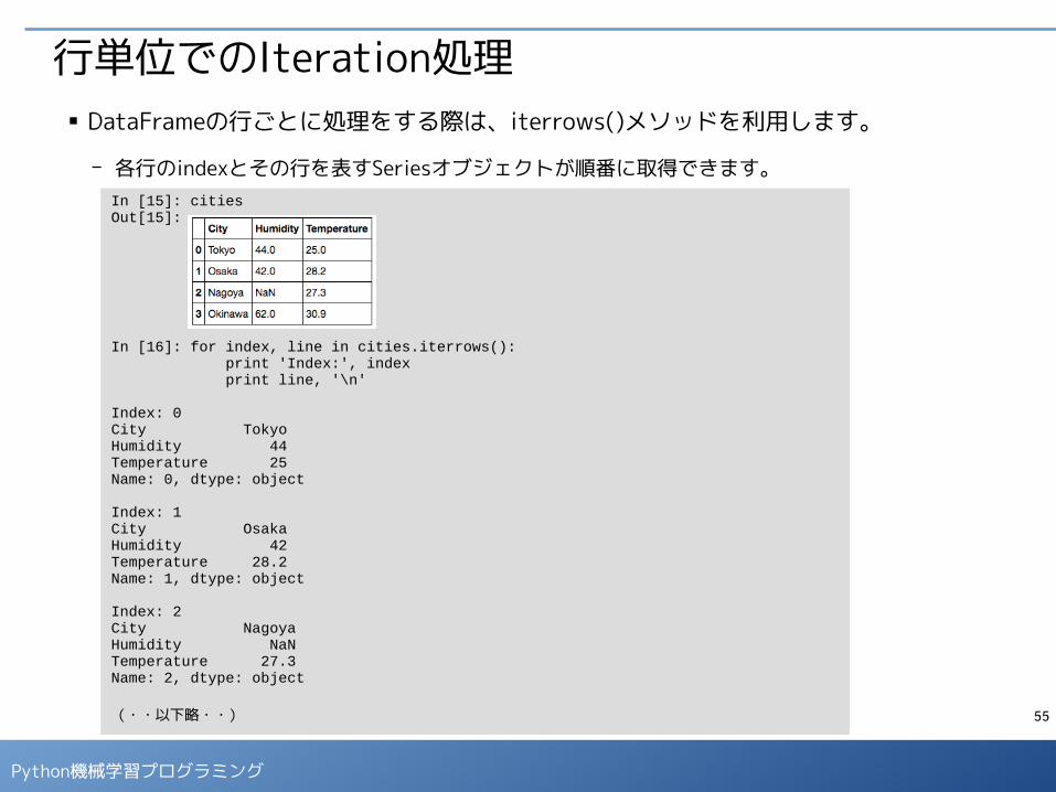
行単位でのIteration処理■ DataFrameの行ごとに処理をする際は、iterrows()メソッドを利用します。
- 各行のindexとその行を表すSeriesオブジェクトが順番に取得できます。In [15]: citiesOut[15]:
In [16]: for index, line in cities.iterrows(): print 'Index:', index print line, '\n' Index: 0City TokyoHumidity 44Temperature 25Name: 0, dtype: object
Index: 1City OsakaHumidity 42Temperature 28.2Name: 1, dtype: object
Index: 2City NagoyaHumidity NaNTemperature 27.3Name: 2, dtype: object
(・・以下略・・)

56
Python機械学習プログラミング
DataFrameから抽出したデータの変更について■ これまでに説明した方法でDataFrameから抽出したオブジェクトは、参照専用として扱
い、値を変更する操作は行わないでください。
- 抽出方法によって、元のDataFrameのオブジェクトを参照している場合とそうでない場合があり、変更の影響範囲が不明確になります。
- 抽出した方の値を変更する際は、copy()メソッドで明示的にオブジェクトのコピーを行います。
In [17]: humidity = cities['Humidity'].copy() humidity[2] = 50 humidityOut[17]: 0 441 422 503 62Name: Humidity, dtype: float64
In [18]: citiesOut[18]:
元のDataFrameは変更されていない
57
Python機械学習プログラミング
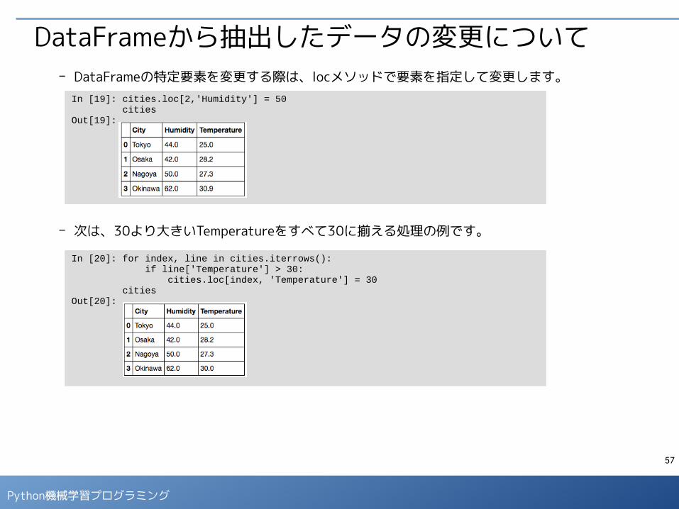
DataFrameから抽出したデータの変更について- DataFrameの特定要素を変更する際は、locメソッドで要素を指定して変更します。
- 次は、30より大きいTemperatureをすべて30に揃える処理の例です。
In [19]: cities.loc[2,'Humidity'] = 50 citiesOut[19]:
In [20]: for index, line in cities.iterrows(): if line['Temperature'] > 30: cities.loc[index, 'Temperature'] = 30 citiesOut[20]:
58
Python機械学習プログラミング
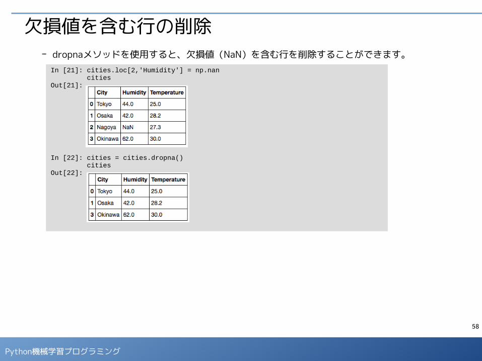
欠損値を含む行の削除- dropnaメソッドを使用すると、欠損値(NaN)を含む行を削除することができます。
In [21]: cities.loc[2,'Humidity'] = np.nan citiesOut[21]:
In [22]: cities = cities.dropna() citiesOut[22]:

59
Python機械学習プログラミング
練習問題■ ノートブック「06-pandas DataFrame-02.ipynb」の末尾にあ
る問題を解いてみましょう。
60
Python機械学習プログラミング
その他のデータフレームの操作
※ このパートでは、ノートブック「07-pandas DataFrame-03.ipynb」を使用します。
61
Python機械学習プログラミング
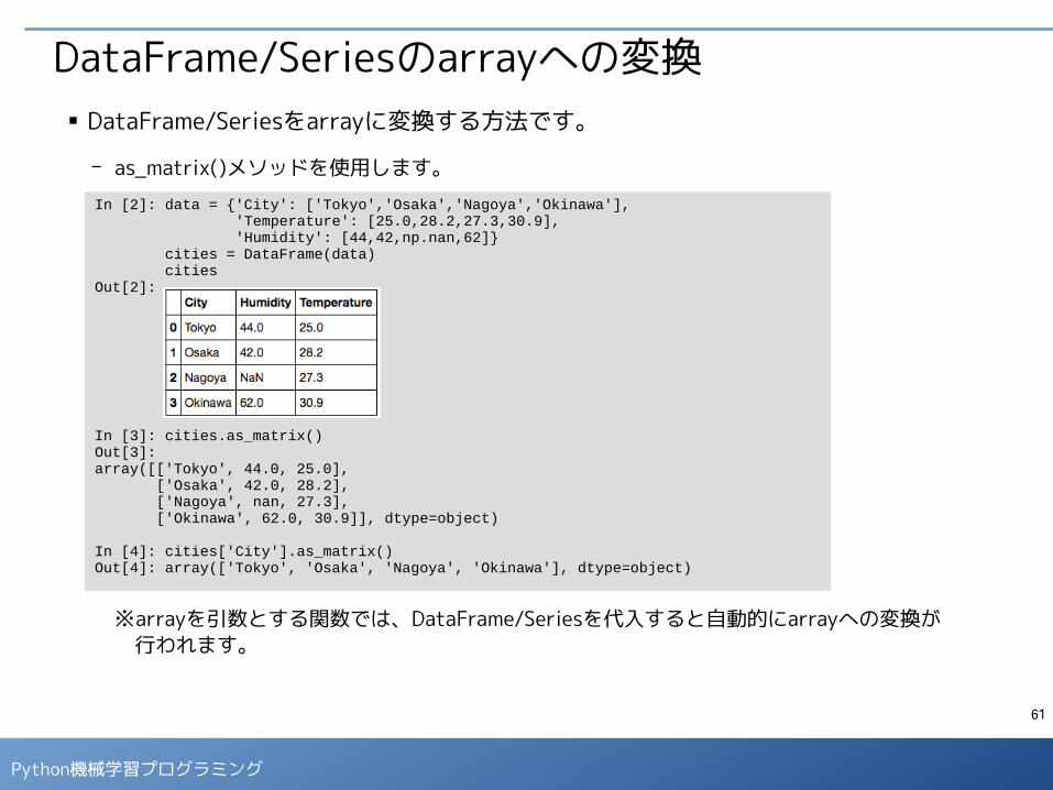
DataFrame/Seriesのarrayへの変換■ DataFrame/Seriesをarrayに変換する方法です。
- as_matrix()メソッドを使用します。
※arrayを引数とする関数では、DataFrame/Seriesを代入すると自動的にarrayへの変換が 行われます。
In [2]: data = {'City': ['Tokyo','Osaka','Nagoya','Okinawa'], 'Temperature': [25.0,28.2,27.3,30.9], 'Humidity': [44,42,np.nan,62]} cities = DataFrame(data) citiesOut[2]:
In [3]: cities.as_matrix()Out[3]: array([['Tokyo', 44.0, 25.0], ['Osaka', 42.0, 28.2], ['Nagoya', nan, 27.3], ['Okinawa', 62.0, 30.9]], dtype=object)
In [4]: cities['City'].as_matrix()Out[4]: array(['Tokyo', 'Osaka', 'Nagoya', 'Okinawa'], dtype=object)
62
Python機械学習プログラミング
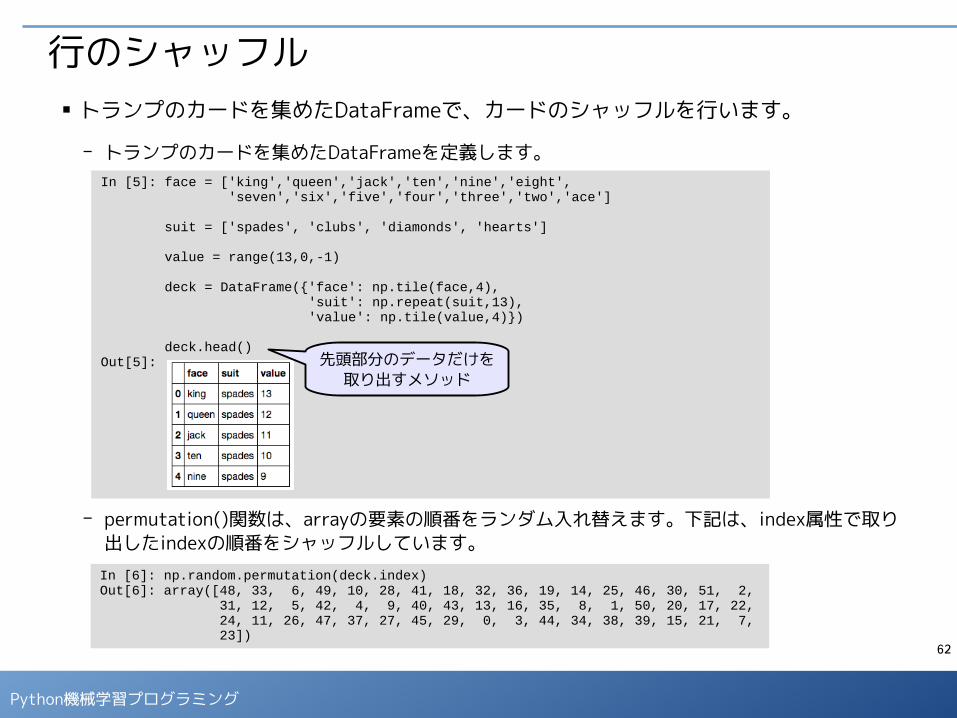
行のシャッフル■ トランプのカードを集めたDataFrameで、カードのシャッフルを行います。
- トランプのカードを集めたDataFrameを定義します。
- permutation()関数は、arrayの要素の順番をランダム入れ替えます。下記は、index属性で取り出したindexの順番をシャッフルしています。
In [5]: face = ['king','queen','jack','ten','nine','eight', 'seven','six','five','four','three','two','ace']
suit = ['spades', 'clubs', 'diamonds', 'hearts']
value = range(13,0,-1)
deck = DataFrame({'face': np.tile(face,4), 'suit': np.repeat(suit,13), 'value': np.tile(value,4)})
deck.head()Out[5]:
In [6]: np.random.permutation(deck.index)Out[6]: array([48, 33, 6, 49, 10, 28, 41, 18, 32, 36, 19, 14, 25, 46, 30, 51, 2, 31, 12, 5, 42, 4, 9, 40, 43, 13, 16, 35, 8, 1, 50, 20, 17, 22, 24, 11, 26, 47, 37, 27, 45, 29, 0, 3, 44, 34, 38, 39, 15, 21, 7, 23])
先頭部分のデータだけを取り出すメソッド
63
Python機械学習プログラミング
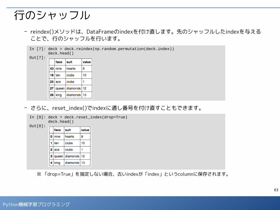
行のシャッフル- reindex()メソッドは、DataFrameのindexを付け直します。先のシャッフルしたindexを与える
ことで、行のシャッフルを行います。
- さらに、reset_index()でindexに通し番号を付け直すこともできます。
※ 「drop=True」を指定しない場合、古いindexが「index」というcolumnに保存されます。
In [7]: deck = deck.reindex(np.random.permutation(deck.index)) deck.head()Out[7]:
In [8]: deck = deck.reset_index(drop=True) deck.head()Out[8]:
64
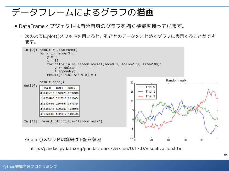
Python機械学習プログラミング
In [9]: result = DataFrame() for c in range(3): y = 0 t = [] for delta in np.random.normal(loc=0.0, scale=1.0, size=100): y += delta t.append(y) result['Trial %d' % c] = t
result.head()Out[9]:
In [10]: result.plot(title='Random walk')
データフレームによるグラフの描画■ DataFrameオブジェクトは自分自身のグラフを描く機能を持っています。
- 次のようにplot()メソッドを用いると、列ごとのデータをまとめてグラフに表示することができます。
※ plot()メソッドの詳細は下記を参照
http://pandas.pydata.org/pandas-docs/version/0.17.0/visualization.html

65
Python機械学習プログラミング
練習問題■ ノートブック「07-pandas DataFrame-03.ipynb」の末尾にあ
る問題を解いてみましょう。

66
Python機械学習プログラミング
最小二乗法のサンプルコード
※ このパートでは、ノートブック「08-Square Error Sample.ipynb」を使用します。
67
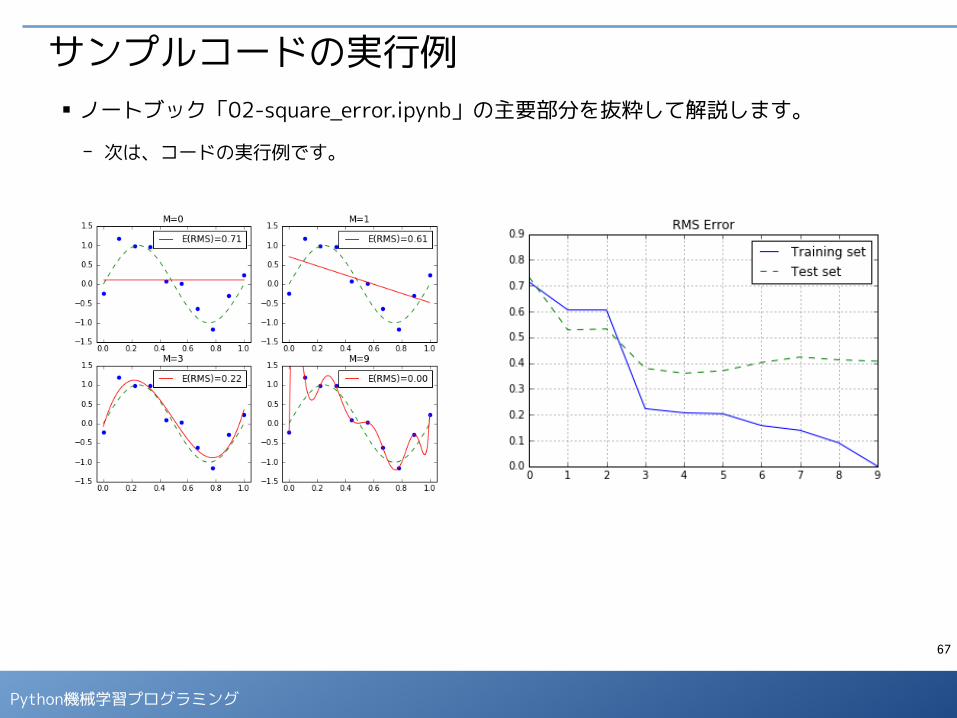
Python機械学習プログラミング
サンプルコードの実行例■ ノートブック「02-square_error.ipynb」の主要部分を抜粋して解説します。
- 次は、コードの実行例です。
68
Python機械学習プログラミング
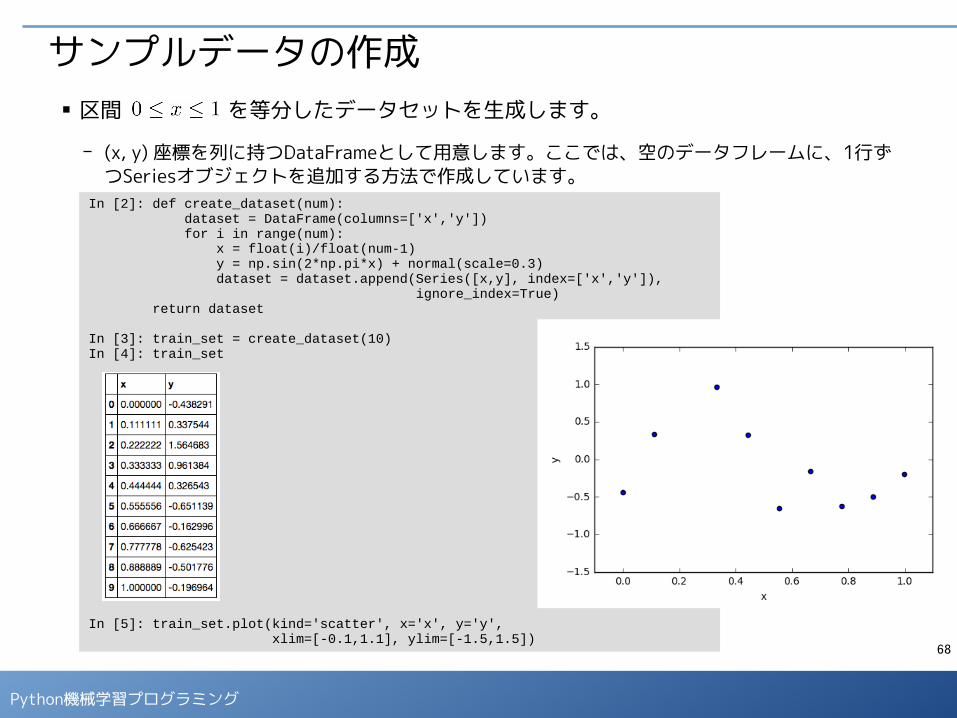
In [2]: def create_dataset(num): dataset = DataFrame(columns=['x','y']) for i in range(num): x = float(i)/float(num-1) y = np.sin(2*np.pi*x) + normal(scale=0.3) dataset = dataset.append(Series([x,y], index=['x','y']), ignore_index=True) return dataset
In [3]: train_set = create_dataset(10)In [4]: train_set
In [5]: train_set.plot(kind='scatter', x='x', y='y', xlim=[-0.1,1.1], ylim=[-1.5,1.5])
サンプルデータの作成■ 区間 を等分したデータセットを生成します。
- (x, y) 座標を列に持つDataFrameとして用意します。ここでは、空のデータフレームに、1行ずつSeriesオブジェクトを追加する方法で作成しています。
69
Python機械学習プログラミング
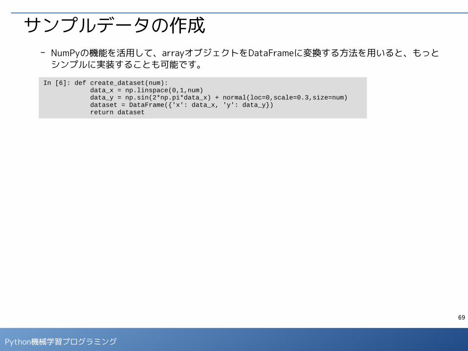
サンプルデータの作成- NumPyの機能を活用して、arrayオブジェクトをDataFrameに変換する方法を用いると、もっと
シンプルに実装することも可能です。
In [6]: def create_dataset(num): data_x = np.linspace(0,1,num) data_y = np.sin(2*np.pi*data_x) + normal(loc=0,scale=0.3,size=num) dataset = DataFrame({'x': data_x, 'y': data_y}) return dataset

70
Python機械学習プログラミング
係数の決定■ 最小二乗法の公式を用いて、多項式の係数を計算します。
- 次の関数では、決定された多項式 と係数 を返しています。
In[7] : def resolve(dataset, m): t = dataset.y
phi = DataFrame() for i in range(0,m+1): p = dataset.x**i p.name="x**%d" % i phi = pd.concat([phi,p], axis=1)
tmp = np.linalg.inv(np.dot(phi.T, phi)) ws = np.dot(np.dot(tmp, phi.T), t)
def f(x): y = 0 for i, w in enumerate(ws): y += w * (x ** i) return y
return (f, ws)
71
Python機械学習プログラミング
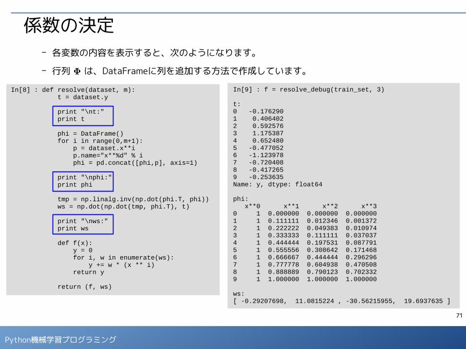
係数の決定- 各変数の内容を表示すると、次のようになります。
- 行列 は、DataFrameに列を追加する方法で作成しています。
In[8] : def resolve(dataset, m): t = dataset.y print "\nt:" print t phi = DataFrame() for i in range(0,m+1): p = dataset.x**i p.name="x**%d" % i phi = pd.concat([phi,p], axis=1)
print "\nphi:" print phi
tmp = np.linalg.inv(np.dot(phi.T, phi)) ws = np.dot(np.dot(tmp, phi.T), t)
print "\nws:" print ws
def f(x): y = 0 for i, w in enumerate(ws): y += w * (x ** i) return y
return (f, ws)
In[9] : f = resolve_debug(train_set, 3)
t: 0 -0.1762901 0.4064022 0.5925763 1.1753874 0.6524805 -0.4770526 -1.1239787 -0.7204088 -0.4172659 -0.253635Name: y, dtype: float64
phi: x**0 x**1 x**2 x**30 1 0.000000 0.000000 0.0000001 1 0.111111 0.012346 0.0013722 1 0.222222 0.049383 0.0109743 1 0.333333 0.111111 0.0370374 1 0.444444 0.197531 0.0877915 1 0.555556 0.308642 0.1714686 1 0.666667 0.444444 0.2962967 1 0.777778 0.604938 0.4705088 1 0.888889 0.790123 0.7023329 1 1.000000 1.000000 1.000000
ws:[ -0.29207698, 11.0815224 , -30.56215955, 19.6937635 ]
72
Python機械学習プログラミング
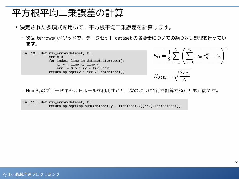
平方根平均二乗誤差の計算■ 決定された多項式を用いて、平方根平均二乗誤差を計算します。
- 次はiterrows()メソッドで、データセット dataset の各要素についての繰り返し処理を行っています。
- NumPyのブロードキャストルールを利用すると、次のように1行で計算することも可能です。
In [10]: def rms_error(dataset, f): err = 0 for index, line in dataset.iterrows(): x, y = line.x, line.y err += 0.5 * (y - f(x))**2 return np.sqrt(2 * err / len(dataset))
In [11]: def rms_error(dataset, f): return np.sqrt(np.sum((dataset.y - f(dataset.x))**2)/len(dataset))
73
Python機械学習プログラミング
In [12]: def show_result(subplot, train_set, m): f = resolve(train_set, m) subplot.set_xlim(-0.05,1.05) subplot.set_ylim(-1.5,1.5) subplot.set_title("M=%d" % m)
# トレーニングセットを表示 subplot.scatter(train_set.x, train_set.y, marker='o', color='blue', label=None)
# 真の曲線を表示 linex = np.linspace(0,1,101) liney = np.sin(2*np.pi*linex) subplot.plot(linex, liney, color='green', linestyle='--')
# 多項式近似の曲線を表示 linex = np.linspace(0,1,101) liney = f(linex) label = "E(RMS)=%.2f" % rms_error(train_set, f) subplot.plot(linex, liney, color='red', label=label) subplot.legend(loc=1)
In [13]: fig = plt.figure(figsize=(8, 6)) for i, m in enumerate([0,1,3,9]): subplot = fig.add_subplot(2,2,i+1) show_result(subplot, train_set, m)
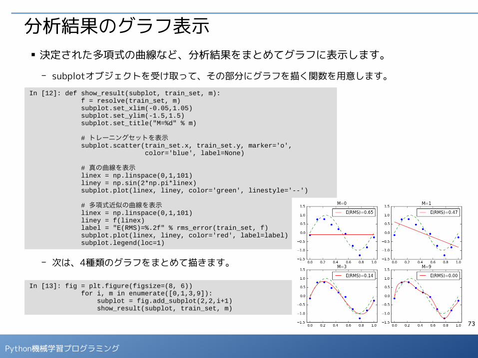
分析結果のグラフ表示■ 決定された多項式の曲線など、分析結果をまとめてグラフに表示します。
- subplotオブジェクトを受け取って、その部分にグラフを描く関数を用意します。
- 次は、4種類のグラフをまとめて描きます。
74
Python機械学習プログラミング
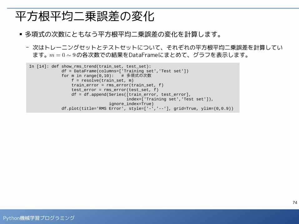
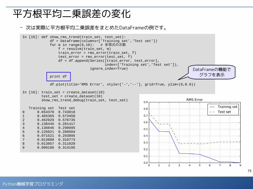
平方根平均二乗誤差の変化■ 多項式の次数にともなう平方根平均二乗誤差の変化を計算します。
- 次はトレーニングセットとテストセットについて、それぞれの平方根平均二乗誤差を計算しています。 の各次数での結果をDataFrameにまとめて、グラフを表示します。
In [14]: def show_rms_trend(train_set, test_set): df = DataFrame(columns=['Training set','Test set']) for m in range(0,10): # 多項式の次数 f = resolve(train_set, m) train_error = rms_error(train_set, f) test_error = rms_error(test_set, f) df = df.append(Series([train_error, test_error], index=['Training set','Test set']), ignore_index=True) df.plot(title='RMS Error', style=['-','--'], grid=True, ylim=(0,0.9))
75
Python機械学習プログラミング
In [15]: def show_rms_trend(train_set, test_set): df = DataFrame(columns=['Training set','Test set']) for m in range(0,10): # 多項式の次数 f = resolve(train_set, m) train_error = rms_error(train_set, f) test_error = rms_error(test_set, f) df = df.append(Series([train_error, test_error], index=['Training set','Test set']), ignore_index=True) print df
df.plot(title='RMS Error', style=['-','--'], grid=True, ylim=(0,0.9))
In [16]: train_set = create_dataset(10) test_set = create_dataset(10) show_rms_trend_debug(train_set, test_set)
Training set Test set0 0.654370 0.7430181 0.465365 0.5734582 0.462929 0.5767353 0.138445 0.2814174 0.136046 0.2909955 0.126021 0.2805046 0.071521 0.2938957 0.013880 0.3107738 0.013857 0.3110289 0.000186 0.314195
平方根平均二乗誤差の変化- 次は実際に平方根平均二乗誤差をまとめたDataFrameの例です。
DataFrameの機能でグラフを表示
76
Python機械学習プログラミング
パーセプトロンのサンプルコード
※ このパートでは、ノートブック「09-Perceptron Sample.ipynb」を使用します。
77
Python機械学習プログラミング
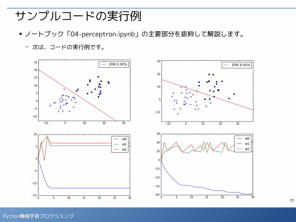
サンプルコードの実行例■ ノートブック「04-perceptron.ipynb」の主要部分を抜粋して解説します。
- 次は、コードの実行例です。
78
Python機械学習プログラミング
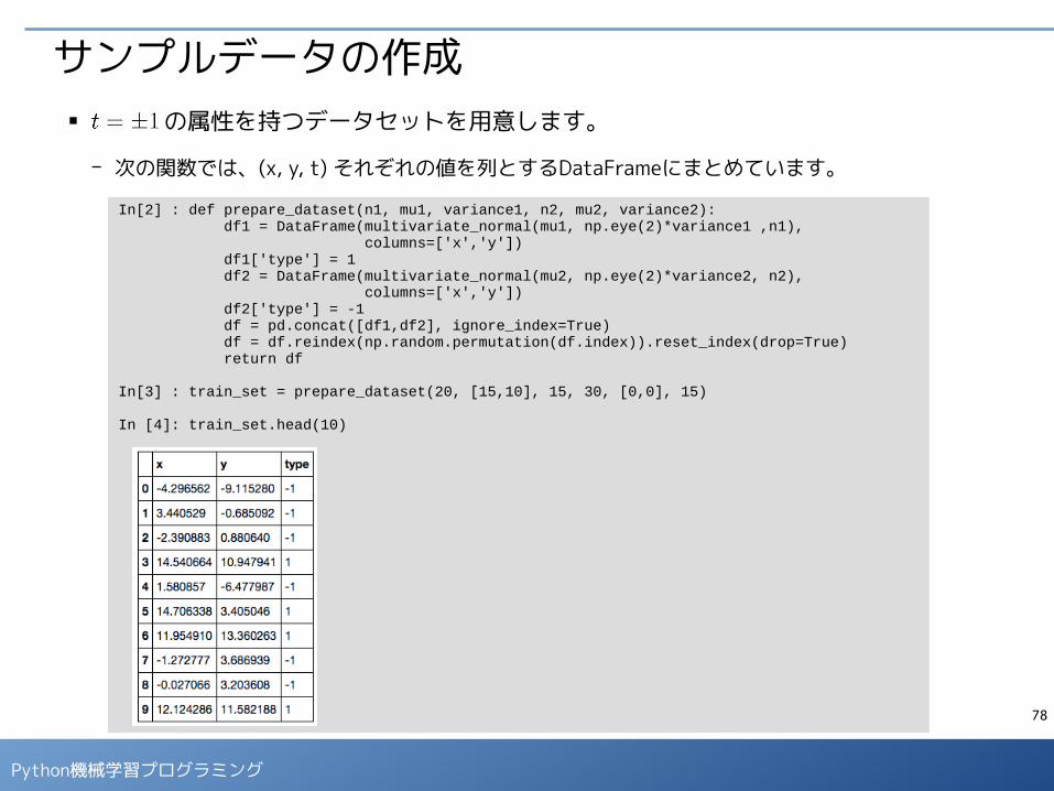
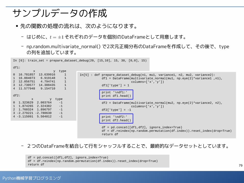
サンプルデータの作成■ の属性を持つデータセットを用意します。
- 次の関数では、(x, y, t) それぞれの値を列とするDataFrameにまとめています。
In[2] : def prepare_dataset(n1, mu1, variance1, n2, mu2, variance2): df1 = DataFrame(multivariate_normal(mu1, np.eye(2)*variance1 ,n1), columns=['x','y']) df1['type'] = 1 df2 = DataFrame(multivariate_normal(mu2, np.eye(2)*variance2, n2), columns=['x','y']) df2['type'] = -1 df = pd.concat([df1,df2], ignore_index=True) df = df.reindex(np.random.permutation(df.index)).reset_index(drop=True) return df
In[3] : train_set = prepare_dataset(20, [15,10], 15, 30, [0,0], 15)
In [4]: train_set.head(10)
79
Python機械学習プログラミング
サンプルデータの作成■ 先の関数の処理の流れは、次のようになります。
- はじめに、 それぞれのデータを個別のDataFrameとして用意します。
- np.random.multivariate_normal() で2次元正規分布のDataFrameを作成して、その後で、typeの列を追加しています。
- 2つのDataFrameを結合して行をシャッフルすることで、最終的なデータセットとしています。
In [6]: train_set = prepare_dataset_debug(20, [15,10], 15, 30, [0,0], 15)
df1: x y type0 16.781857 13.639916 11 16.884073 6.919148 12 12.056751 4.794741 13 12.730577 14.388435 14 11.577948 9.154710 1
df2: x y type0 1.323629 2.003764 -11 1.874265 2.324382 -12 1.760324 1.896797 -13 -2.279221 -2.780630 -14 -3.115091 5.504012 -1
In[5] : def prepare_dataset_debug(n1, mu1, variance1, n2, mu2, variance2): df1 = DataFrame(multivariate_normal(mu1, np.eye(2)*variance1 ,n1), columns=['x','y']) df1['type'] = 1
print '\ndf1:' print df1.head()
df2 = DataFrame(multivariate_normal(mu2, np.eye(2)*variance2, n2), columns=['x','y']) df2['type'] = -1
print '\ndf2:' print df2.head()
df = pd.concat([df1,df2], ignore_index=True) df = df.reindex(np.random.permutation(df.index)).reset_index(drop=True) return df
df = pd.concat([df1,df2], ignore_index=True)df = df.reindex(np.random.permutation(df.index)).reset_index(drop=True)return df
80
Python機械学習プログラミング
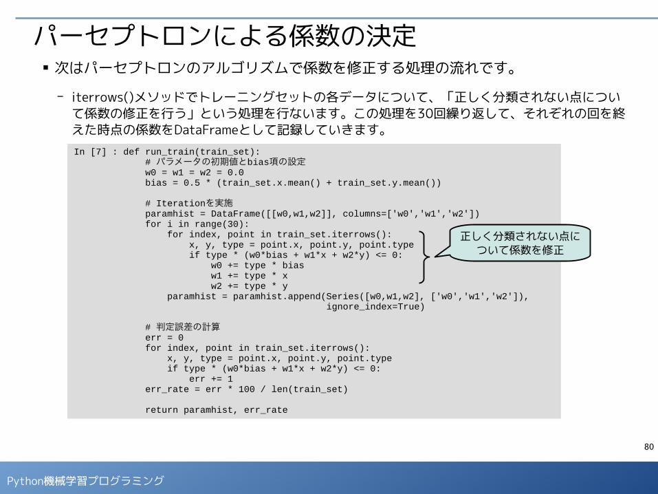
パーセプトロンによる係数の決定■ 次はパーセプトロンのアルゴリズムで係数を修正する処理の流れです。
- iterrows()メソッドでトレーニングセットの各データについて、「正しく分類されない点について係数の修正を行う」という処理を行ないます。この処理を30回繰り返して、それぞれの回を終えた時点の係数をDataFrameとして記録していきます。 In [7] : def run_train(train_set): # パラメータの初期値とbias項の設定 w0 = w1 = w2 = 0.0 bias = 0.5 * (train_set.x.mean() + train_set.y.mean())
# Iterationを実施 paramhist = DataFrame([[w0,w1,w2]], columns=['w0','w1','w2']) for i in range(30): for index, point in train_set.iterrows(): x, y, type = point.x, point.y, point.type if type * (w0*bias + w1*x + w2*y) <= 0: w0 += type * bias w1 += type * x w2 += type * y paramhist = paramhist.append(Series([w0,w1,w2], ['w0','w1','w2']), ignore_index=True) # 判定誤差の計算 err = 0 for index, point in train_set.iterrows(): x, y, type = point.x, point.y, point.type if type * (w0*bias + w1*x + w2*y) <= 0: err += 1 err_rate = err * 100 / len(train_set) return paramhist, err_rate
正しく分類されない点について係数を修正

81
Python機械学習プログラミング
In [8]: paramhist, err_rate = run_train(train_set) paramhist.head(10)
In [9]: paramhist.plot.legend(loc=1)
パーセプトロンによる係数の決定- 係数の変化を記録したDataFrameの様子です。DataFrameの機能を利用して、グラフを描くこと
ができます。
82
Python機械学習プログラミング
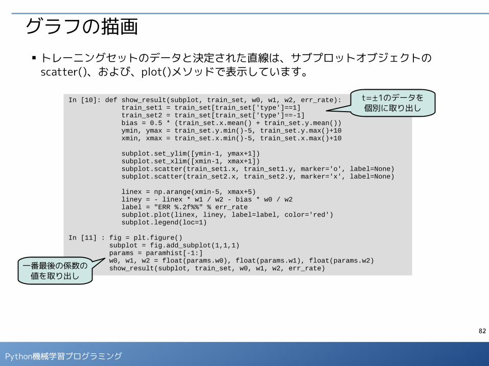
グラフの描画■ トレーニングセットのデータと決定された直線は、サブプロットオブジェクトの
scatter()、および、plot()メソッドで表示しています。
In [10]: def show_result(subplot, train_set, w0, w1, w2, err_rate): train_set1 = train_set[train_set['type']==1] train_set2 = train_set[train_set['type']==-1] bias = 0.5 * (train_set.x.mean() + train_set.y.mean()) ymin, ymax = train_set.y.min()-5, train_set.y.max()+10 xmin, xmax = train_set.x.min()-5, train_set.x.max()+10
subplot.set_ylim([ymin-1, ymax+1]) subplot.set_xlim([xmin-1, xmax+1]) subplot.scatter(train_set1.x, train_set1.y, marker='o', label=None) subplot.scatter(train_set2.x, train_set2.y, marker='x', label=None)
linex = np.arange(xmin-5, xmax+5) liney = - linex * w1 / w2 - bias * w0 / w2 label = "ERR %.2f%%" % err_rate subplot.plot(linex, liney, label=label, color='red') subplot.legend(loc=1)
In [11] : fig = plt.figure() subplot = fig.add_subplot(1,1,1) params = paramhist[-1:] w0, w1, w2 = float(params.w0), float(params.w1), float(params.w2) show_result(subplot, train_set, w0, w1, w2, err_rate)
t=±1のデータを個別に取り出し
一番最後の係数の値を取り出し

83
Python機械学習プログラミング
参考資料
84
Python機械学習プログラミング
参考資料
■ 『Pythonによるデータ分析入門 ―― NumPy、pandasを使ったデータ処理』 WesMcKinney(著)、小林 儀匡、鈴木 宏尚、瀬戸山 雅人、滝口 開資、野上 大介(翻訳)、オライリージャパン(2013)
- NumPyやpandasなど、データ解析に使用する標準的なPythonライブラリの使用方法を解説しています。
■ 『Think Stats 第2版 ―プログラマのための統計入門』 Allen B. Downey(著)、 黒川 利明 (翻訳)、黒川 洋 (翻訳)、オライリージャパン(2015)
- 統計解析の実例をPythonで実装しながら解説しています。
85
Python機械学習プログラミング
メモとしてお使いください

Machine Learning for Everyone Else
Thank You!