UV Visi NI FIRMIR

Russell JohnstonCollaborators: Mattia Vaccari, Matt Jarvis, Mat Smith, Matt Prescott, Elodie Giovannoli

The evolving relation between SFR and M* in the VIDEO survey since z = 3

I. A bit of background

II. Creating our star-forming sample

III. Results part 1 - the star-forming main sequence

IV. Results part 2 - simulations and implications

A Bit of Background

• How do galaxies evolve?

• What are the physical processes driving that evolution?

a

To probe star formation histories of galaxies, the key components are:

M! yr-1

Measure of the present

activity of the galaxy

M! !

Measure of the past activity of the

galaxy.

Galaxy spectra is the sum of the different components:

!STARS !

GAS !

DUST !

We need access to the full stellar emission to determine

these quantities

young old dust

SFR M★

star formation ratestellar mass

Estimating Star Formation Rates

• UV - emission dominated by young massive short-lived star.

Estimating Star Formation Rates

Estimating Star Formation Rates

➡ Dust in galaxies absorbs UV and optical photons !➡ Which is then re-emitted at infrared wavelengths

Visible Infrared

Dust

Log 1

0[λF

λ(t)

] (er

g s-

1 M

!-1

)Wavelength (μm)

• UV - emission dominated by young massive short-lived star.

• UV+IR - Account for dust attenuation in the UV.

• Nebular emission lines - , ,

• Radio continuum emission and stacking.

• SED Modelling e.g. CIGALE and MAGPHYS

H↵ O[II] O[III]

Estimating Star Formation Rates

Multi-wavelength Observations

UV Visible

NIR

FIRMIR

The SFR-Mass “Main Sequence”

Noeske et al. 2007

Daddi et al. 2007Elbaz et al. 2007

DEEP2, K-band imaging and Spitzer MIPS 24 µm

GOODS, SDSS, Spitzer 3.6, 4.8 µm MIPS 24 µm UV, radio, mid and far IR

An Emerging Picture

➡ SF galaxies follow tight SFR-Mass relation.

➡ SFR increases with Mass as a Power-law.

➡ Intrinsic scatter

0.2 . �MS . 0.35

➡ Strong evolution in the n o r m a l i s a t i o n w i t h redshift

➡ Measurements of slope vary wildly in literature

0.2 < ↵ < 1.2

SFR / M↵⇤

CREATING OUR STAR FORMING SAMPLEII.

The VIDEO Survey VISTA Deep Extragalactic Observations

( Jarvis et al. 2013 )

VIDEO

Spitzer SWIRE

CFHTLS-D1

UKIDSS-UDS

!➡ 12 deg^2 !➡ (NIR): Z, Y, J, H, K

s

➡ Visible: ugriz (CFHTLS)

➡ zphot

< 4.0

➡ zphot

obtained from !

LePhare

➡ SERVS (Spitzer Extragalactic Representative Volume Survey, Mauduit et al. 2012)

IRAC 1 - 3.6 µm IRAC 2 - 4.5 µm

Joint selection

then matched to

➡ SWIRE (Spitzer Wide-Area Extragalactic, Lonsdale et al. 2003)

IRAC 1 - 5.8 µm IRAC 2 - 8.0 µm

➡ HerMES (Herschel Multi-tiered Extragalactic Survey, Olivier et al. 2012)

SPIRE 250, 350 and 500 µm

MIPS 24, 70 and 160 µm

Matching to Multi-wavelength data

First Things First

• SFR indicator

• Mass Completeness

• Cosmic Variance

• Star-forming selection criteria

• Calibration

Code Investigating GALaxy Emission (CIGALE) (Burgarella et al. 2005; Noll et al. 2009b)

CIGALE INPUT• Photometric broad-bands

• Star Formation History

• Dust Attenuation

• IR Library

CIGALE OUTPUT• SFR

• M*

• LDUST

• .... etc...

Combines UV-optical stellar SED with dust emission in IR

to conserve energy balance between dust absorbed emission

and its re-emission in IR

Wavelength (µm)SPIRE

HerschelSpitzer

ZYJHK

VIDEO

ugriz

CFHTLS

MIPSIRAC

exponentially decreasing tau models

Kroupa IMF

PEGASE

FIR part of the spectrum

Dale & Helou (2002) !64 templates

6 AGN models

Code Investigating GALaxy Emission (CIGALE) (Burgarella et al. 2005; Noll et al. 2009b)

0.0 0.5 1.0 1.5 2.0 2.5 3.0redshift (zph)

0

500

1000

1500

2000

2500

3000

3500

4000

4500

N

VIDEO + CFHTLS + SERVS

0.0 0.5 1.0 1.5 2.0 2.5 3.0redshift (zph)

0

50

100

150

200

250

300

350

400

450MIPS (24 µm)IRAC (5.8 µm)SPIRE (250 µm)

Matching to Multi-wavelength data

�0.5

0.0

0.5

1.0

1.5

2.0

2.5

3.0

3.5

log(

SFR

2)[M

�y�

1 ]

8.5

9.0

9.5

10.0

10.5

11.0

11.5

log(

M⇤ 2)

[M�

]

�1.0 �0.5 0.0 0.5 1.0 1.5 2.0 2.5 3.0 3.5log(SFR1)[M� y�1]

�1.0

�0.5

0.0

0.5

1.0

log(

SFR

1/S

FR2)

8.0 8.5 9.0 9.5 10.0 10.5 11.0 11.5 12.0log(M⇤

1) [M�]

�1.0

�0.5

0.0

0.5

1.0

log(

M⇤ 1/

M⇤ 2)

0.3

0.6

0.9

1.2

1.5

1.8

2.1

2.4

2.7

reds

hift

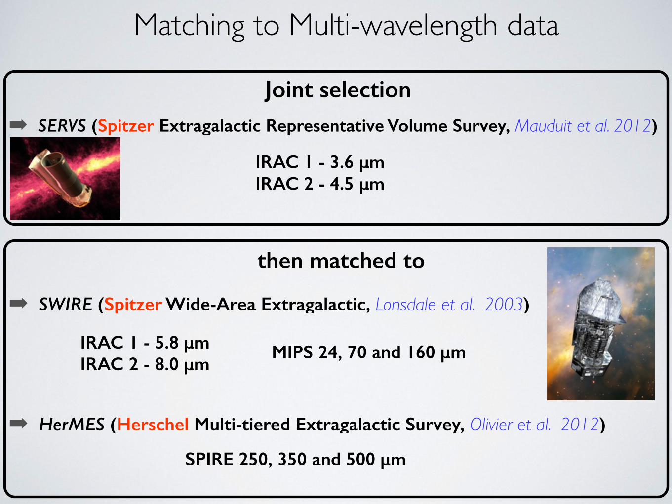
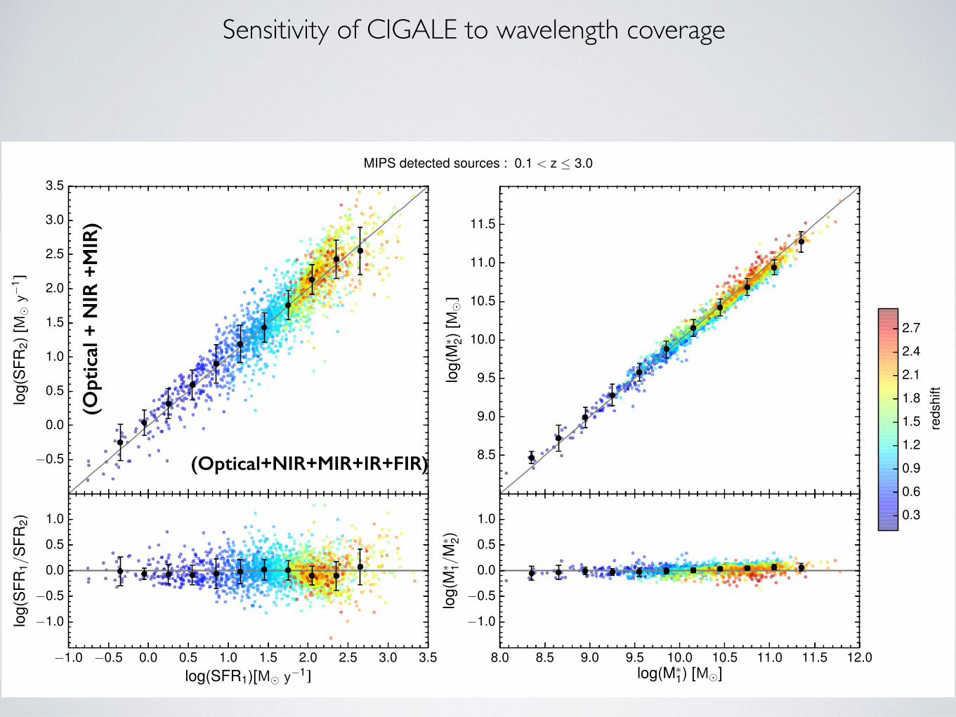
MIPS detected sources : 0.1 < z 3.0

Sensitivity of CIGALE to wavelength coverage

(Opt

ical

+ N

IR +

MIR

)

(Optical+NIR+MIR+IR+FIR)

Mass Completeness Limits • Joint selection in Ks with SERVS 3.6 & 4.5 µm

log10(Mlim) = log10(M⇤) + 0.4(Ks �K lims )

- [Ilbert et al. (2013)]

0.5 1.0 1.5 2.0 2.5 3.0redshift

0.0

0.1

0.2

0.3

0.4

0.5

cosm

icva

rianc

e(�

v)

Dark Matter8.5 < log(M⇤) 9.09.0 < log(M⇤) 9.59.5 < log(M⇤) 10.010.0 < log(M⇤) 10.510.5 < log(M⇤) 11.011.0 < log(M⇤) 11.5

Cosmic Variance • VIDEO currently only covers 1 sq. deg

• Uncertainty in observed number density of galaxies arising from the underlying large-scale density fluctuations.

Moster et al. (2011)‘GETCV’

• Determined using predictions from CDM and theory and galaxy bias

Selecting Star Forming Galaxies • Common to perform rest-frame colour selection e.g. UVJ, U-B, BzK, u-g

• or sigma-clip

• mixture: NUV-r and r-J Ilbert et al. 2014

Schreiber et al. 2015

(Magnelli et al. 2014, Santini et al. 2009)

(e.g. Daddi et al. 2007, Whitaker et al. 2014, Rodighiero et al. 2011,)

• Avoids selecting the bluest galaxies

Colour cut (u-r)

0.5 1.0 1.5 2.0 2.5 3.0100

600

1100

1600

2100

2600

N

0.5 1.0 1.5 2.0 2.5 3.0

U � R

8

9

10

11

log(

M⇤ /

M�

)

Selecting Star Forming Galaxies

1.0 1.1 1.2 1.3 1.4 1.5100

600

1100

1600

2100

N

1.0 1.1 1.2 1.3 1.4 1.5

D4000

8

9

10

11

log(

M⇤ /

M�

)

D4000 break

Selecting Star Forming Galaxies

D4000<1.3

• An output from CIGALE. • Related to the age of a stellar population. • low D4000 index = younger SP • high D4000 index = older SP

Aratio of the average flux per frequency unit of the

wavelength ranges 4000–4100 Å and 3850–3950 Å Balogh et al. 1999

Calibrating the Main Sequence

• Comparing your results to other works is very tricky! Wavelength coverage/selection

SFR estimation (L-SFR relation)

Initial mass function (IMF)

Stellar population synthesis models (SPS)

Star forming galaxy selection

Star formation histories (SFH) [difficult to correct/calibrate] Extinction Metallicities Adopted cosmology Dust attenuation Photometric redshifts Incompleteness

!!

(see Speagle et al. 2014)

|{z} affects normalisation

affects slope

III. RESULTS PART 1 THE STAR-FORMING MAIN SEQUENCE

The Star Forming Main Sequence

log(SFR) = ↵ log(M⇤) + �

log(SFR) = A1 +A2 log(M⇤) + A3[log(M⇤)]2

(e.g. Noeske et al. 2007, Daddi et al. 2007, Elbaz et al. 2007, Santini et al. 2009, Heinis et al. 2014)

SFR = ↵

✓M⇤

1011 M�

◆�

log[SFR(z)] = ↵(z)[log(M⇤)� 10.5] + �(z)

↵(z) = ↵1 + ↵2z

�(z) = �1 + �2z + �3z2

where,

(e.g. Magnelli et al 2014, Whitaker et al 2014)

(e.g. Whitaker et al 2012)

Modelling the Data

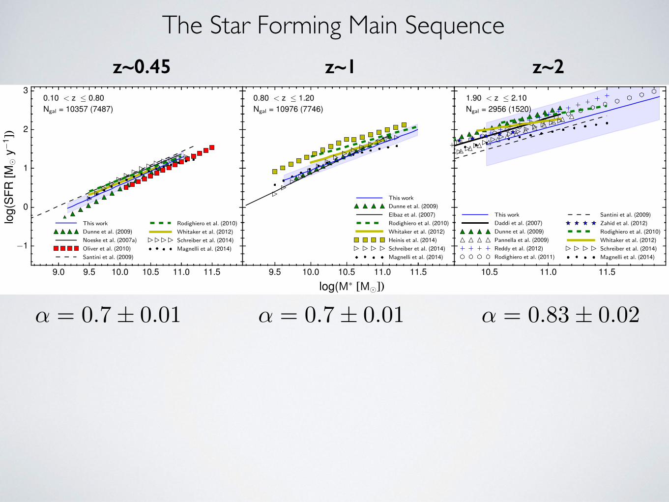
9.0 9.5 10.0 10.5 11.0 11.5

�1

0

1

2

3

This work

Dunne et al. (2009)Noeske et al. (2007a)Oliver et al. (2010)Santini et al. (2009)

Rodighiero et al. (2010)Whitaker et al. (2012)Schreiber et al. (2014)Magnelli et al. (2014)

0.10 < z 0.80Ngal = 10357 (7487)

9.5 10.0 10.5 11.0 11.5

This work

Dunne et al. (2009)Elbaz et al. (2007)Rodighiero et al. (2010)Whitaker et al. (2012)Heinis et al. (2014)Schreiber et al. (2014)Magnelli et al. (2014)

0.80 < z 1.20Ngal = 10976 (7746)

10.5 11.0 11.5

This work

Daddi et al. (2007)Dunne et al. (2009)Pannella et al. (2009)Reddy et al. (2012)Rodighiero et al. (2011)

Santini et al. (2009)Zahid et al. (2012)Rodighiero et al. (2010)Whitaker et al. (2012)Schreiber et al. (2014)Magnelli et al. (2014)

1.90 < z 2.10Ngal = 2956 (1520)

log(M⇤ [M�])

log(

SFR

[M�

y�1 ]

)

z~0.45 z~1 z~2

The Star Forming Main Sequence

↵ = 0.7± 0.01 ↵ = 0.7± 0.01 ↵ = 0.83± 0.02

0.0 0.5 1.0 1.5 2.0 2.5 3.0

redshift

�0.2

0.0

0.2

0.4

0.6

0.8

1.0

↵

This work (D4000)Daddi et al. (2007)Santini et al. (2009)Rodighiero et al. (2011)Noeske et al. (2007a)

Elbaz et al. (2007)Dunne et al. (2009)Pannella et al. (2009)Rodighiero et al. (2010)Oliver et al. (2010)

Zahid et al. (2012)Reddy et al. (2012)Whitaker et al. (2012)Whitaker et al. (2014)Whitaker et al. (2014)

The Star Forming Main Sequence

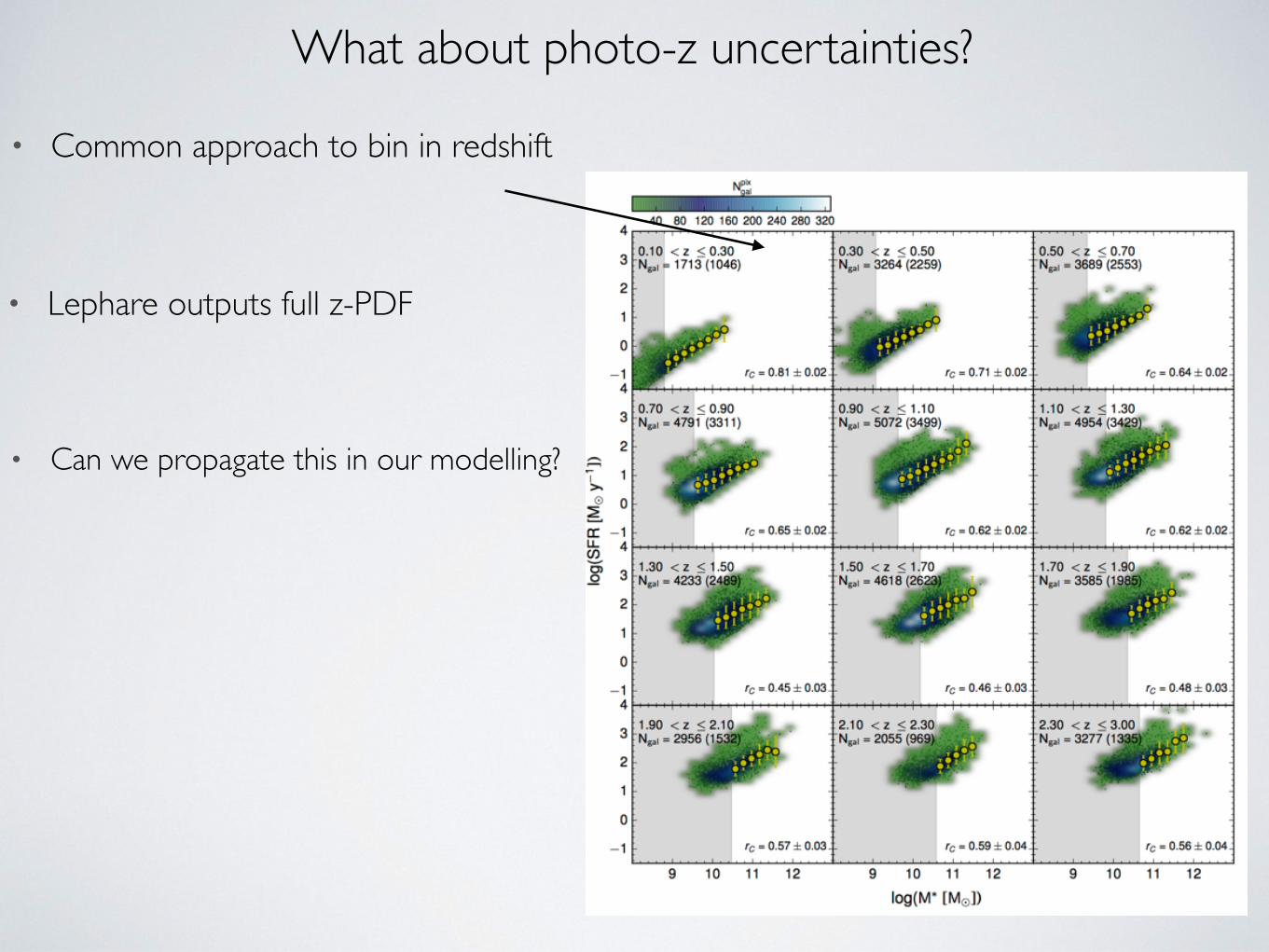
What about photo-z uncertainties?

• Common approach to bin in redshift

• Lephare outputs full z-PDF

• Can we propagate this in our modelling?

0.2

0.4

0.6

0.8

1.0pr

obab

ility

�0.5

0.0

0.5

1.0

0.2 0.4 0.6 0.8 1.0

0.2 0.3 0.4 0.5 0.6 0.7redshift

8.4

8.6

8.8

9.0

9.2

9.4

9.6

9.8

log(

M⇤

[M�

])

0.2 0.4 0.6 0.8 1.0

log(

SFR

[M�

y�1 ]

)

probability

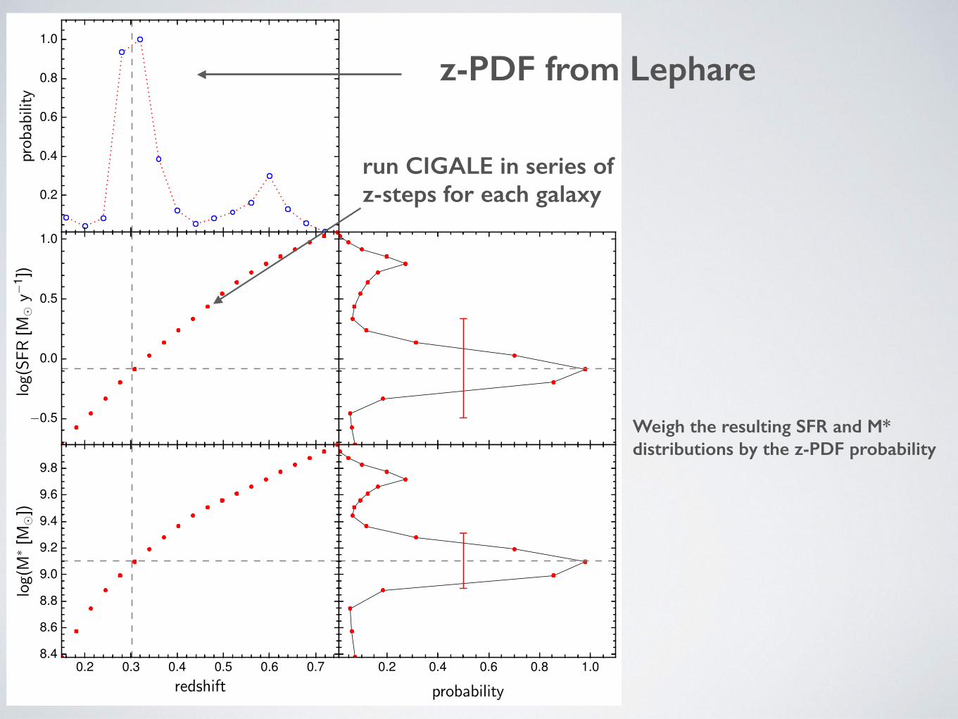
z-PDF from Lephare

run CIGALE in series of z-steps for each galaxy

Weigh the resulting SFR and M* distributions by the z-PDF probability

log10[SFR(z)] = ↵(z)[log10(M⇤)� 10.5] + �(z),

↵(z) = ↵1 + ↵2z, and

�(z) = �1 + �2z + �3z2

median constraints - DOES NOT INCLUDE zPDF uncertainties

‘all data’ constraints - INCLUDES zPDF uncertainties

(Whitaker et al 2012)

log10[SFR(z)] = ↵(z)[log10(M⇤)� 10.5] + �(z),

↵(z) = ↵1 + ↵2z, and

�(z) = �1 + �2z + �3z2

OUR median constraints

Whitaker et al. (2012) (medians)

High mass SFR turn-off?

Whitaker et al. (2014)stacking in MIPS 24µm

Tasca et al. (2014) [VUDS]

Magnelli et al. (2014) [PACS, HerMES]

9.8 10.0 10.2 10.4 10.6 10.8 11.0 11.2 11.4log(M⇤ [M�])

0.5

1.0

1.5

2.0

log(

SFR

[M�

y�1 ]

)

D4000 < 1.30D4000 < 1.35Whitaker et al. (2014)

1.00 < z 1.50

0.0 0.5 1.0 1.5 2.0 2.5 3.0redshift

0.0

0.2

0.4

0.6

0.8

1.0

↵

This work (D4000)This work (u � r)

Star-Forming Selection Effects

�10.5

�9.5

�8.5

�7.5

9.85 < M⇤ < 10.15sSFR / (1 + z)3.56±0.01

Feulner et al. (2005)Noeske et al. (2007a)Dunne et al. (2009)

Whitaker et al. (2012)Salmi et al. (2012)

Ilbert et al. (2013)Heinis et al. (2014)

�10.5

�9.5

�8.5

�7.5

10.15 < M⇤ < 10.45sSFR / (1 + z)3.09±0.03

Zheng et al. (2007)Daddi et al. (2007)Kajisawa et al. (2009)

Rodighiero et al. (2010)Karim et al. (2011)Ilbert et al. (2013)

Zwart et al. (2014)Tasca et al. (2014)Schreiber et al. (2014)

�10.5

�9.5

�8.5

�7.5

10.45 < M⇤ < 10.65sSFR / (1 + z)2.60±0.04

Noeske et al. (2007a)Dunne et al. (2009)Karim et al. (2011)

Whitaker et al. (2012)Salmi et al. (2012)

Ilbert et al. (2013)Heinis et al. (2014)

�10.5

�9.5

�8.5

�7.5

10.65 < M⇤ < 10.85sSFR / (1 + z)2.15±0.04

Zheng et al. (2007)Daddi et al. (2007)Kajisawa et al. (2009)Rodighiero et al. (2010)

Ilbert et al. (2013)Zwart et al. (2014)Schreiber et al. (2014)

0.0 0.5 1.0 1.5 2.0 2.5 3.0�10.5

�9.5

�8.5

�7.5

10.85 < M⇤ < 11.15sSFR / (1 + z)2.13±0.06

Feulner et al. (2005)Karim et al. (2011)Whitaker et al. (2012)Heinis et al. (2014)

redshift

log(

sSFR

[y�

1 ])

• At between we find , consistent to Tasca et al. (2014)

log10(sSFR) = log10(SFR)� log10(M⇤)

• Mass dependent evolution out to z<1.4 , similar to that of Ilbert et al. (2014)

• General flattening off beyond

• We model this by

sSFR / (1 + z)�

Evolution of the Specific Star Formation Rate

0.4 < z < 2.46

z > 2

M⇤ ⇠ 10.5

� = 2.60± 0.04

IV. RESULTS PART II SIMULATIONS AND IMPLICATIONS

!

Hydrodynamical: Scaling relations:

➡Horizon - Dubois et al. (2014)

➡Ilustris - Sparre et al. (2014)

➡Davé et al (2013)➡Mitra et al. (2014)

- Equilibrium Model-

What Can Simulations Tell Us?

Star formation gas cooling and heating feedback from stellar winds, supernovae and AGN

analytical - constrained to observed data

Describes motion of gas into and out of galaxies - baryon cycle. 8 free parameters

➡Behroozi et al. (2013)

- HOD-stellar mass-halo mass scaling relation 15 free parameters

9 10 11

0

1

2

3This workIllustris, Sparre et al. (2014)Mitra et al. (2014)Horizon, Dubois et al. (2014)Behroozi et al. (2013)Dave et al. (2013)

z = 1

9 10 11

z = 2

9 10 11

0

1

2

3This work

Horizon � (with cut)

Horizon � (no cut)

9 10 11log(M⇤ [M�])

log(

SFR

[M�

y�1 ]

)

�10.5

�9.5

�8.5

�7.5

9.85 < M⇤ < 10.15

Behroozi et al. (2013)Mitra et al. (2014)Illustris � Sparre et al. (2014)Horizon � Dubois et al. (2014)

�10.5

�9.5

�8.5

�7.5

10.15 < M⇤ < 10.45

Mitra et al. (2014)Horizon � Dubois et al. (2014)

�10.5

�9.5

�8.5

�7.5

10.45 < M⇤ < 10.65

Behroozi et al. (2013)Mitra et al. (2014)Illustris � Sparre et al. (2014)Horizon � Dubois et al. (2014)

�10.5

�9.5

�8.5

�7.5

10.65 < M⇤ < 10.85

Mitra et al. (2014)Horizon � Dubois et al. (2014)

0.0 0.5 1.0 1.5 2.0 2.5 3.0�10.5

�9.5

�8.5

�7.5

10.85 < M⇤ < 11.15

Behroozi et al. (2013)Illustris � Sparre et al. (2014)Mitra et al. (2014)Horizon � Dubois et al. (2014)

redshift

log(

sSFR

[y�

1 ])

• Hydro show lower normalisation by factor of 2-6 between 0.5<z<~3.0

• Good agreement with scaling relation approaches.

Implications

• Discrepancy between hydro/SAMs and observations well known

• Oversimplified gas accretion modelling?

• Systematic offsets in gas cooling rates?

• Insufficient sub-grid models that control star formation

and stellar feedback?

(Daddi et al. 2007; Elbaz et al. 2007; Santini et al. 2009; Damen et al. 2009b; Davé et al. 2013; Sparre et al. 2014; Genel et al. 2014; Tasca et al. 2014)

• Currently this remains an unresolved issue:

Implications

• Equilibrium model [Mitra et al. (2014)] does not explicitly model: • halos, • cooling, • mergers or • a disk star formation law

• Parameterises the motion of gas into and out of galaxies

• Is continual smooth accretion regulated by continual outflows a key driver in the overall growth of SFGs?