Embed Size (px)
Citation preview
Andrea Cavallucci - 2015
A guide to Microsoft Excel
Thanks:
howtogeek.comsupport.office.microsoft.com www.chandoo.org excel-easy.com excelforum.com slideshare.net techonthenet.com exceluser.com gcflearnfree.org
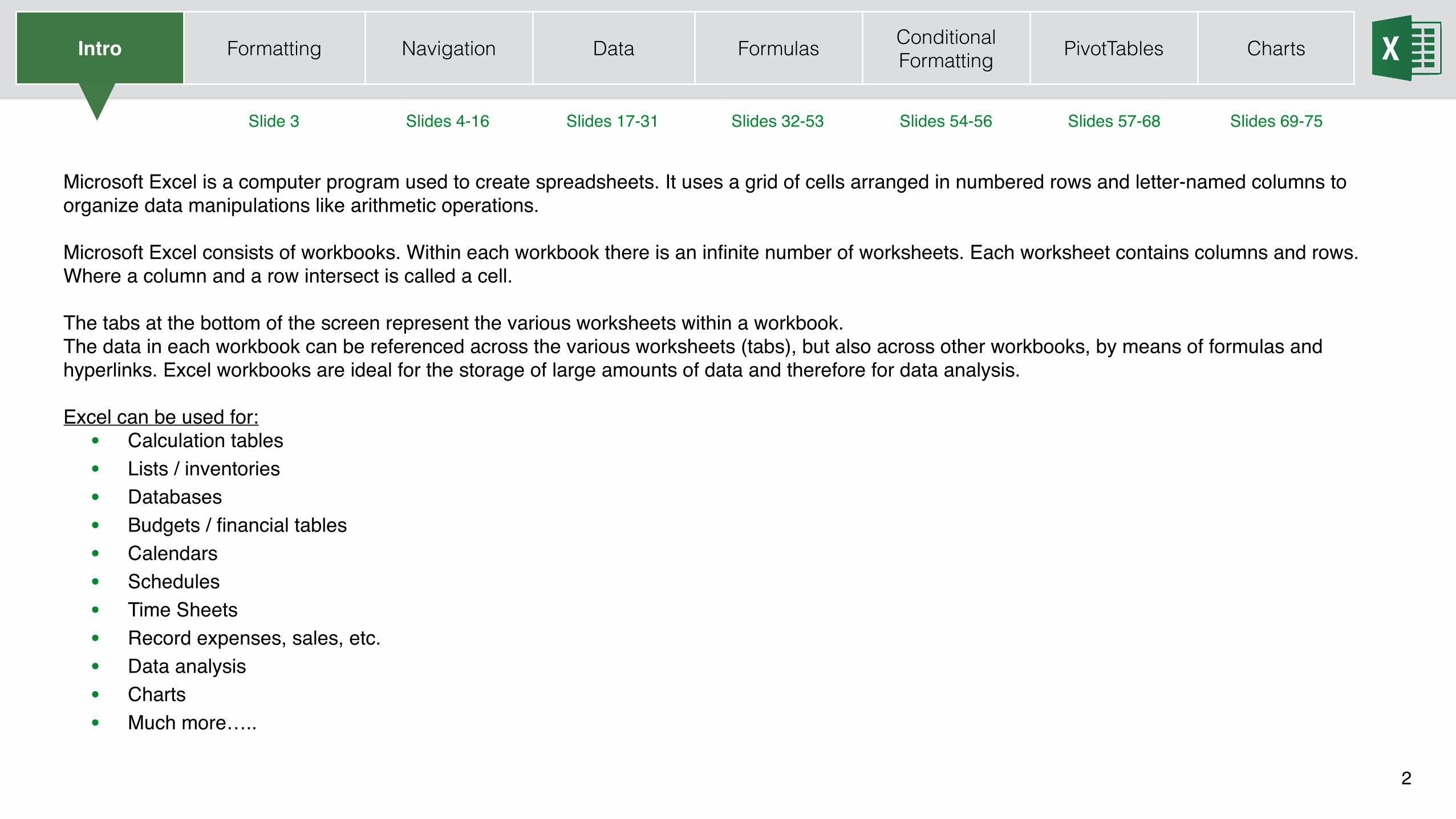
Microsoft Excel is a computer program used to create spreadsheets. It uses a grid of cells arranged in numbered rows and letter-named columns to organize data manipulations like arithmetic operations.
Microsoft Excel consists of workbooks. Within each workbook there is an infinite number of worksheets. Each worksheet contains columns and rows. Where a column and a row intersect is called a cell.
The tabs at the bottom of the screen represent the various worksheets within a workbook.The data in each workbook can be referenced across the various worksheets (tabs), but also across other workbooks, by means of formulas and hyperlinks. Excel workbooks are ideal for the storage of large amounts of data and therefore for data analysis.
Excel can be used for:• Calculation tables• Lists / inventories• Databases• Budgets / financial tables• Calendars• Schedules• Time Sheets• Record expenses, sales, etc.• Data analysis• Charts• Much more…..
Intro Formatting Navigation Data Formulas Conditional Formatting PivotTables Charts
2
Slide 3 Slides 4-16 Slides 17-31 Slides 32-53 Slides 54-56 Slides 57-68 Slides 69-75
Intro Formatting Navigation Data Formulas Conditional Formatting PivotTables Charts
3
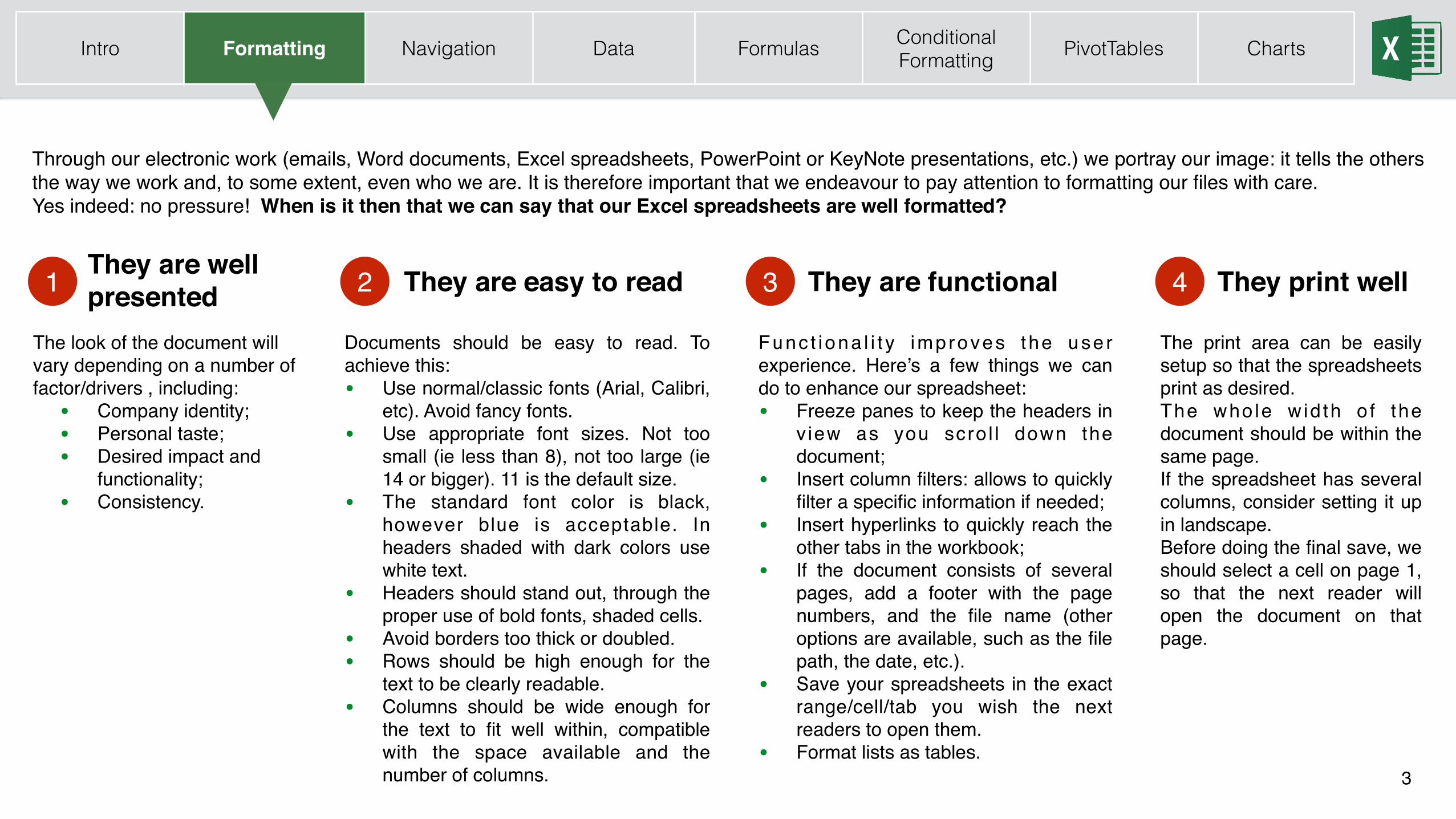
Through our electronic work (emails, Word documents, Excel spreadsheets, PowerPoint or KeyNote presentations, etc.) we portray our image: it tells the others the way we work and, to some extent, even who we are. It is therefore important that we endeavour to pay attention to formatting our files with care. Yes indeed: no pressure! When is it then that we can say that our Excel spreadsheets are well formatted?
They are well presented They are easy to read They are functional They print well
The look of the document will vary depending on a number of factor/drivers , including:
• Company identity;• Personal taste;• Desired impact and
functionality;• Consistency.
Documents should be easy to read. To achieve this:• Use normal/classic fonts (Arial, Calibri,
etc). Avoid fancy fonts.• Use appropriate font sizes. Not too
small (ie less than 8), not too large (ie 14 or bigger). 11 is the default size.
• The standard font color is black, however blue is acceptable. In headers shaded with dark colors use white text.
• Headers should stand out, through the proper use of bold fonts, shaded cells.
• Avoid borders too thick or doubled.• Rows should be high enough for the
text to be clearly readable.• Columns should be wide enough for
the text to fit well within, compatible with the space available and the number of columns.
Func t i ona l i t y improves the use r experience. Here’s a few things we can do to enhance our spreadsheet:• Freeze panes to keep the headers in
v iew as you scro l l down the document;
• Insert column filters: allows to quickly filter a specific information if needed;
• Insert hyperlinks to quickly reach the other tabs in the workbook;
• If the document consists of several pages, add a footer with the page numbers, and the file name (other options are available, such as the file path, the date, etc.).
• Save your spreadsheets in the exact range/cell/tab you wish the next readers to open them.
• Format lists as tables.
The print area can be easily setup so that the spreadsheets print as desired.The who le w id th o f the document should be within the same page.If the spreadsheet has several columns, consider setting it up in landscape.Before doing the final save, we should select a cell on page 1, so that the next reader will open the document on that page.
1 2 3 4
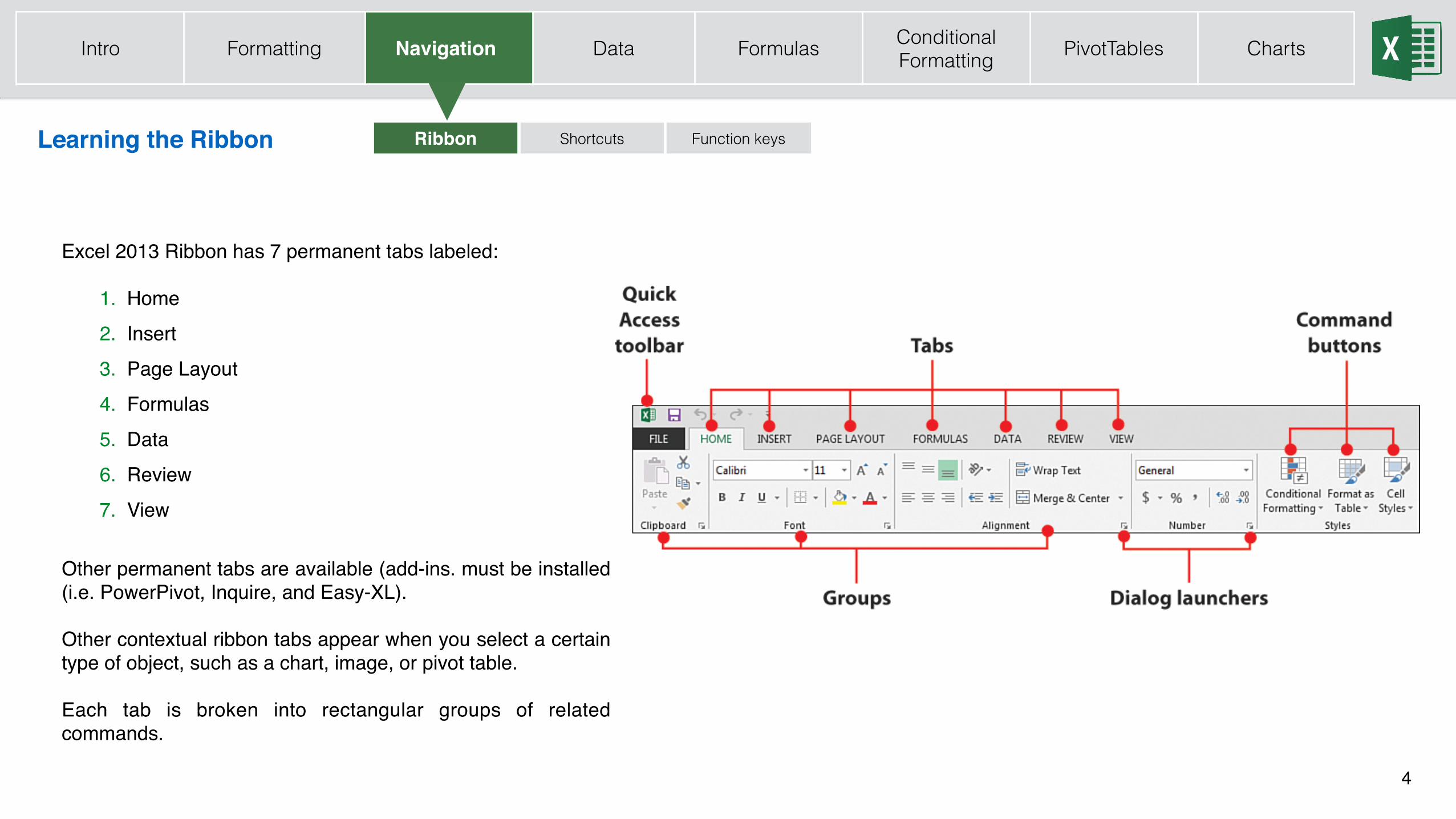
Excel 2013 Ribbon has 7 permanent tabs labeled:
1. Home2. Insert3. Page Layout4. Formulas5. Data6. Review7. View
Other permanent tabs are available (add-ins. must be installed (i.e. PowerPivot, Inquire, and Easy-XL).
Other contextual ribbon tabs appear when you select a certain type of object, such as a chart, image, or pivot table.
Each tab is broken into rectangular groups of related commands.
Ribbon Shortcuts Function keysLearning the Ribbon
Intro Formatting Navigation Data Formulas Conditional Formatting PivotTables Charts
4
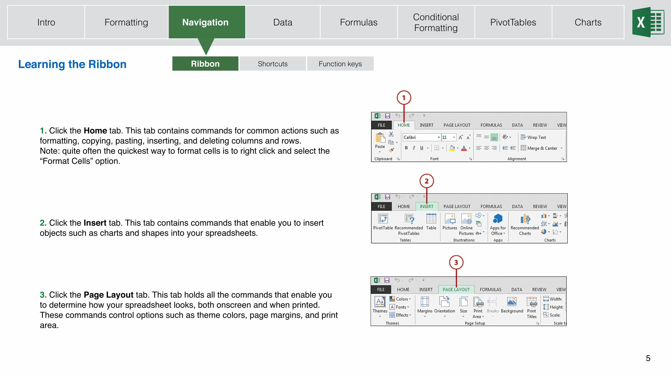
1. Click the Home tab. This tab contains commands for common actions such as formatting, copying, pasting, inserting, and deleting columns and rows. Note: quite often the quickest way to format cells is to right click and select the “Format Cells” option.
2. Click the Insert tab. This tab contains commands that enable you to insert objects such as charts and shapes into your spreadsheets.
3. Click the Page Layout tab. This tab holds all the commands that enable you to determine how your spreadsheet looks, both onscreen and when printed. These commands control options such as theme colors, page margins, and print area.
Learning the Ribbon Ribbon Shortcuts Function keys
5
Intro Formatting Navigation Data Formulas Conditional Formatting PivotTables Charts
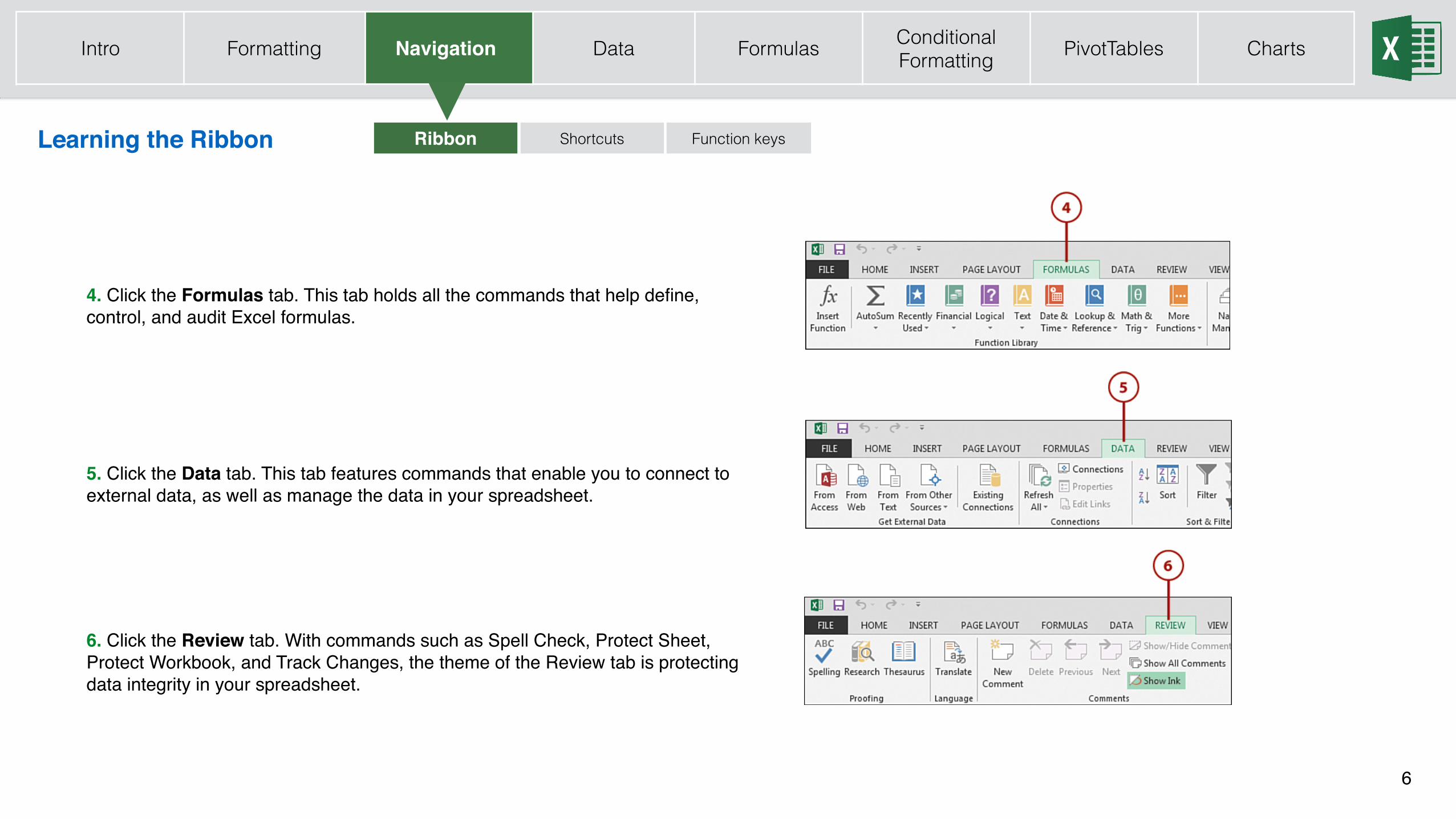
4. Click the Formulas tab. This tab holds all the commands that help define, control, and audit Excel formulas.
5. Click the Data tab. This tab features commands that enable you to connect to external data, as well as manage the data in your spreadsheet.
6. Click the Review tab. With commands such as Spell Check, Protect Sheet, Protect Workbook, and Track Changes, the theme of the Review tab is protecting data integrity in your spreadsheet.
Learning the Ribbon Ribbon Shortcuts Function keys
6
Intro Formatting Navigation Data Formulas Conditional Formatting PivotTables Charts
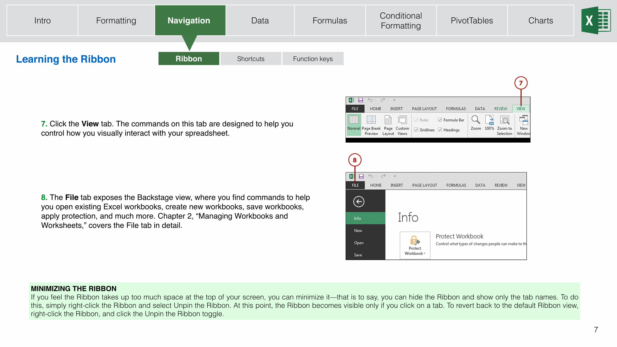
7. Click the View tab. The commands on this tab are designed to help you control how you visually interact with your spreadsheet.
8. The File tab exposes the Backstage view, where you find commands to help you open existing Excel workbooks, create new workbooks, save workbooks, apply protection, and much more. Chapter 2, “Managing Workbooks and Worksheets,” covers the File tab in detail.
MINIMIZING THE RIBBONIf you feel the Ribbon takes up too much space at the top of your screen, you can minimize it—that is to say, you can hide the Ribbon and show only the tab names. To do this, simply right-click the Ribbon and select Unpin the Ribbon. At this point, the Ribbon becomes visible only if you click on a tab. To revert back to the default Ribbon view, right-click the Ribbon, and click the Unpin the Ribbon toggle.
Learning the Ribbon Ribbon Shortcuts Function keys
7
Intro Formatting Navigation Data Formulas Conditional Formatting PivotTables Charts
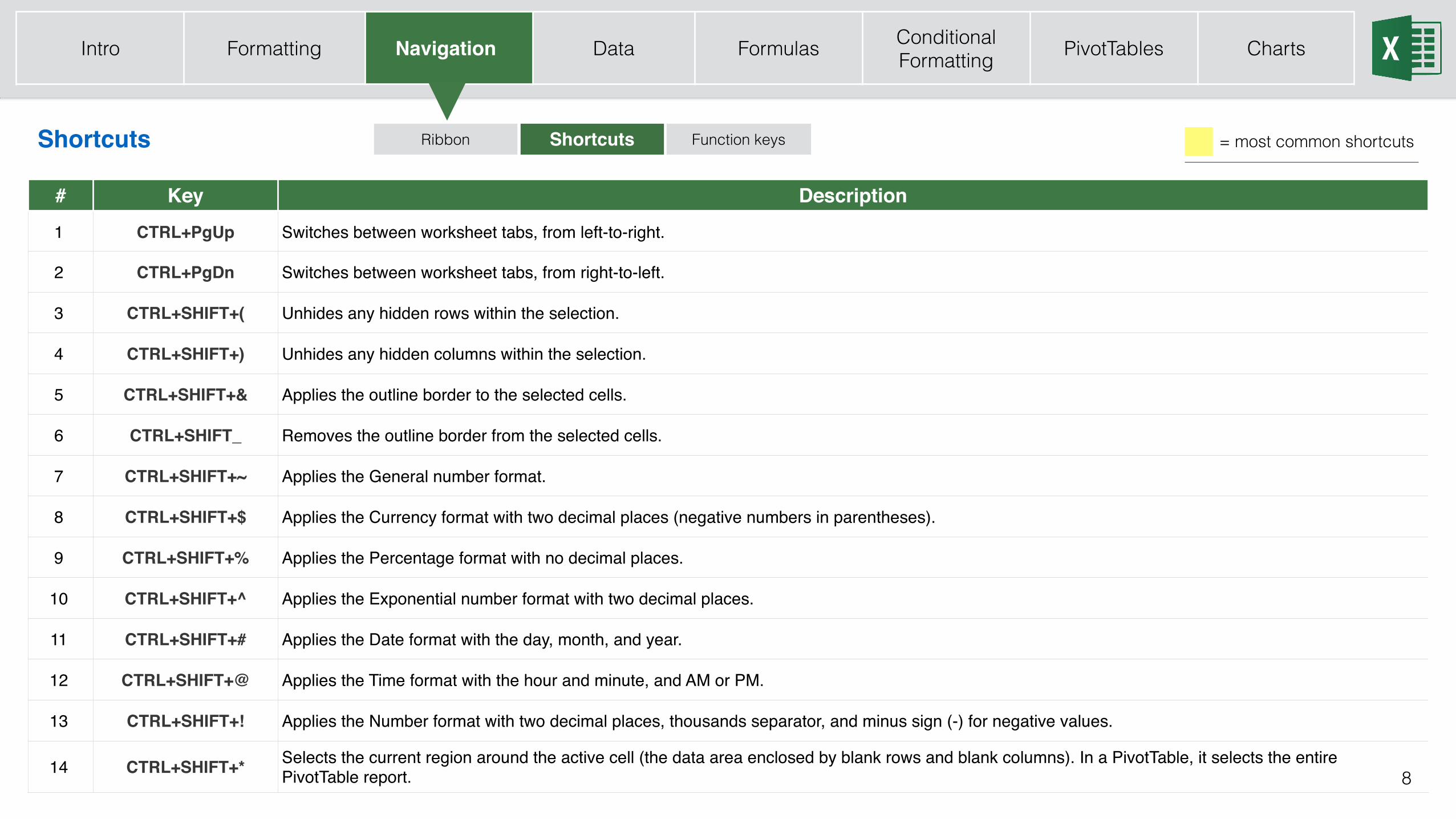
# Key Description
1 CTRL+PgUp Switches between worksheet tabs, from left-to-right.
2 CTRL+PgDn Switches between worksheet tabs, from right-to-left.
3 CTRL+SHIFT+( Unhides any hidden rows within the selection.
4 CTRL+SHIFT+) Unhides any hidden columns within the selection.
5 CTRL+SHIFT+& Applies the outline border to the selected cells.
6 CTRL+SHIFT_ Removes the outline border from the selected cells.
7 CTRL+SHIFT+~ Applies the General number format.
8 CTRL+SHIFT+$ Applies the Currency format with two decimal places (negative numbers in parentheses).
9 CTRL+SHIFT+% Applies the Percentage format with no decimal places.
10 CTRL+SHIFT+^ Applies the Exponential number format with two decimal places.
11 CTRL+SHIFT+# Applies the Date format with the day, month, and year.
12 CTRL+SHIFT+@ Applies the Time format with the hour and minute, and AM or PM.
13 CTRL+SHIFT+! Applies the Number format with two decimal places, thousands separator, and minus sign (-) for negative values.
14 CTRL+SHIFT+* Selects the current region around the active cell (the data area enclosed by blank rows and blank columns). In a PivotTable, it selects the entire PivotTable report. 8
Ribbon Shortcuts Function keysShortcutsShortcuts = most common shortcuts
Intro Formatting Navigation Data Formulas Conditional Formatting PivotTables Charts
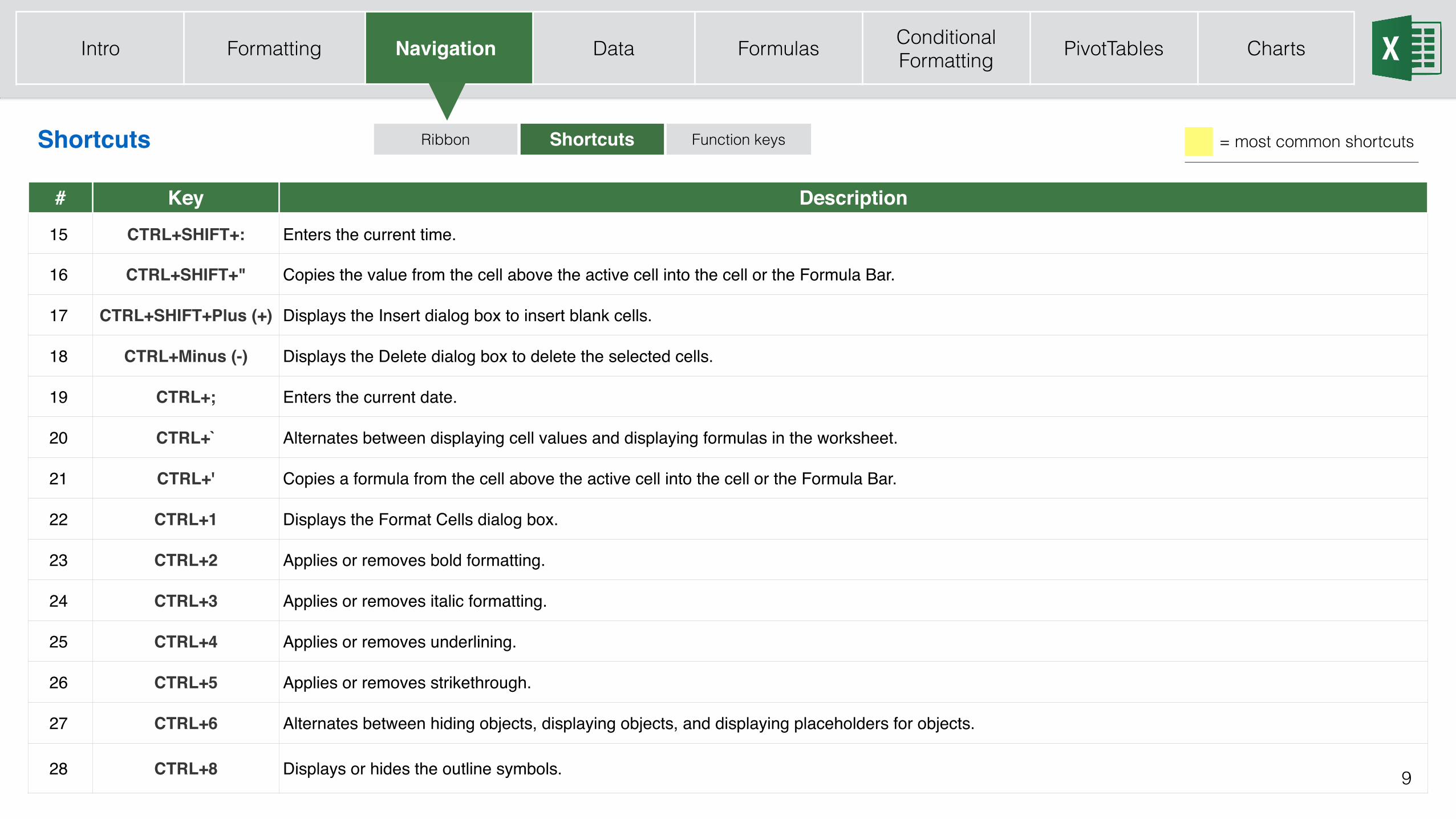
# Key Description
15 CTRL+SHIFT+: Enters the current time.
16 CTRL+SHIFT+" Copies the value from the cell above the active cell into the cell or the Formula Bar.
17 CTRL+SHIFT+Plus (+) Displays the Insert dialog box to insert blank cells.
18 CTRL+Minus (-) Displays the Delete dialog box to delete the selected cells.
19 CTRL+; Enters the current date.
20 CTRL+` Alternates between displaying cell values and displaying formulas in the worksheet.
21 CTRL+' Copies a formula from the cell above the active cell into the cell or the Formula Bar.
22 CTRL+1 Displays the Format Cells dialog box.
23 CTRL+2 Applies or removes bold formatting.
24 CTRL+3 Applies or removes italic formatting.
25 CTRL+4 Applies or removes underlining.
26 CTRL+5 Applies or removes strikethrough.
27 CTRL+6 Alternates between hiding objects, displaying objects, and displaying placeholders for objects.
28 CTRL+8 Displays or hides the outline symbols. 9
Ribbon Shortcuts Function keysShortcuts = most common shortcuts
Intro Formatting Navigation Data Formulas Conditional Formatting PivotTables Charts
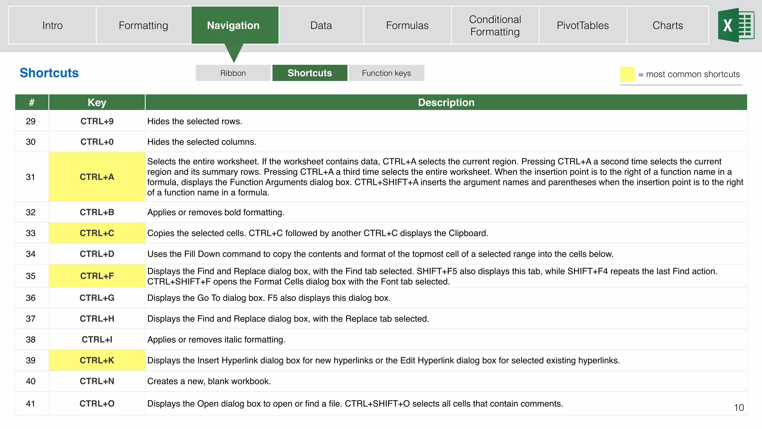
# Key Description29 CTRL+9 Hides the selected rows.
30 CTRL+0 Hides the selected columns.
31 CTRL+ASelects the entire worksheet. If the worksheet contains data, CTRL+A selects the current region. Pressing CTRL+A a second time selects the current region and its summary rows. Pressing CTRL+A a third time selects the entire worksheet. When the insertion point is to the right of a function name in a formula, displays the Function Arguments dialog box. CTRL+SHIFT+A inserts the argument names and parentheses when the insertion point is to the right of a function name in a formula.
32 CTRL+B Applies or removes bold formatting.
33 CTRL+C Copies the selected cells. CTRL+C followed by another CTRL+C displays the Clipboard.
34 CTRL+D Uses the Fill Down command to copy the contents and format of the topmost cell of a selected range into the cells below.
35 CTRL+F Displays the Find and Replace dialog box, with the Find tab selected. SHIFT+F5 also displays this tab, while SHIFT+F4 repeats the last Find action.CTRL+SHIFT+F opens the Format Cells dialog box with the Font tab selected.
36 CTRL+G Displays the Go To dialog box. F5 also displays this dialog box.
37 CTRL+H Displays the Find and Replace dialog box, with the Replace tab selected.
38 CTRL+I Applies or removes italic formatting.
39 CTRL+K Displays the Insert Hyperlink dialog box for new hyperlinks or the Edit Hyperlink dialog box for selected existing hyperlinks.
40 CTRL+N Creates a new, blank workbook.
41 CTRL+O Displays the Open dialog box to open or find a file. CTRL+SHIFT+O selects all cells that contain comments. 10
= most common shortcutsRibbon Shortcuts Function keysShortcuts
Intro Formatting Navigation Data Formulas Conditional Formatting PivotTables Charts
# Key Description
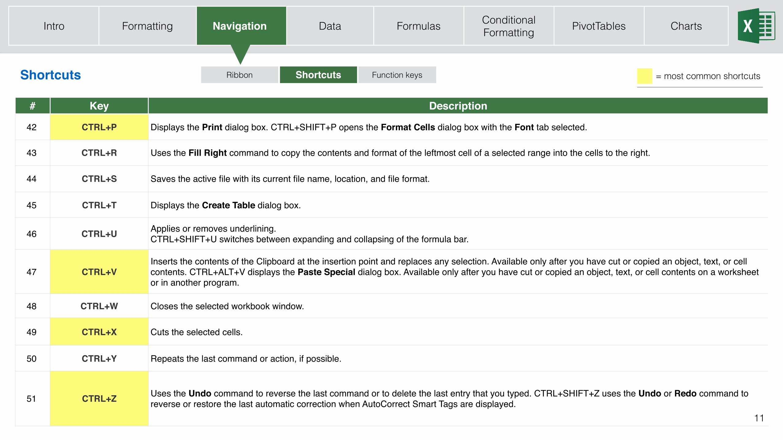
42 CTRL+P Displays the Print dialog box. CTRL+SHIFT+P opens the Format Cells dialog box with the Font tab selected.
43 CTRL+R Uses the Fill Right command to copy the contents and format of the leftmost cell of a selected range into the cells to the right.
44 CTRL+S Saves the active file with its current file name, location, and file format.
45 CTRL+T Displays the Create Table dialog box.
46 CTRL+U Applies or removes underlining.CTRL+SHIFT+U switches between expanding and collapsing of the formula bar.
47 CTRL+VInserts the contents of the Clipboard at the insertion point and replaces any selection. Available only after you have cut or copied an object, text, or cell contents. CTRL+ALT+V displays the Paste Special dialog box. Available only after you have cut or copied an object, text, or cell contents on a worksheet or in another program.
48 CTRL+W Closes the selected workbook window.
49 CTRL+X Cuts the selected cells.
50 CTRL+Y Repeats the last command or action, if possible.
51 CTRL+Z Uses the Undo command to reverse the last command or to delete the last entry that you typed. CTRL+SHIFT+Z uses the Undo or Redo command to reverse or restore the last automatic correction when AutoCorrect Smart Tags are displayed.
11
Ribbon Shortcuts Function keysShortcuts = most common shortcuts
Intro Formatting Navigation Data Formulas Conditional Formatting PivotTables Charts
12
Ribbon Shortcuts Function keys
Key Description
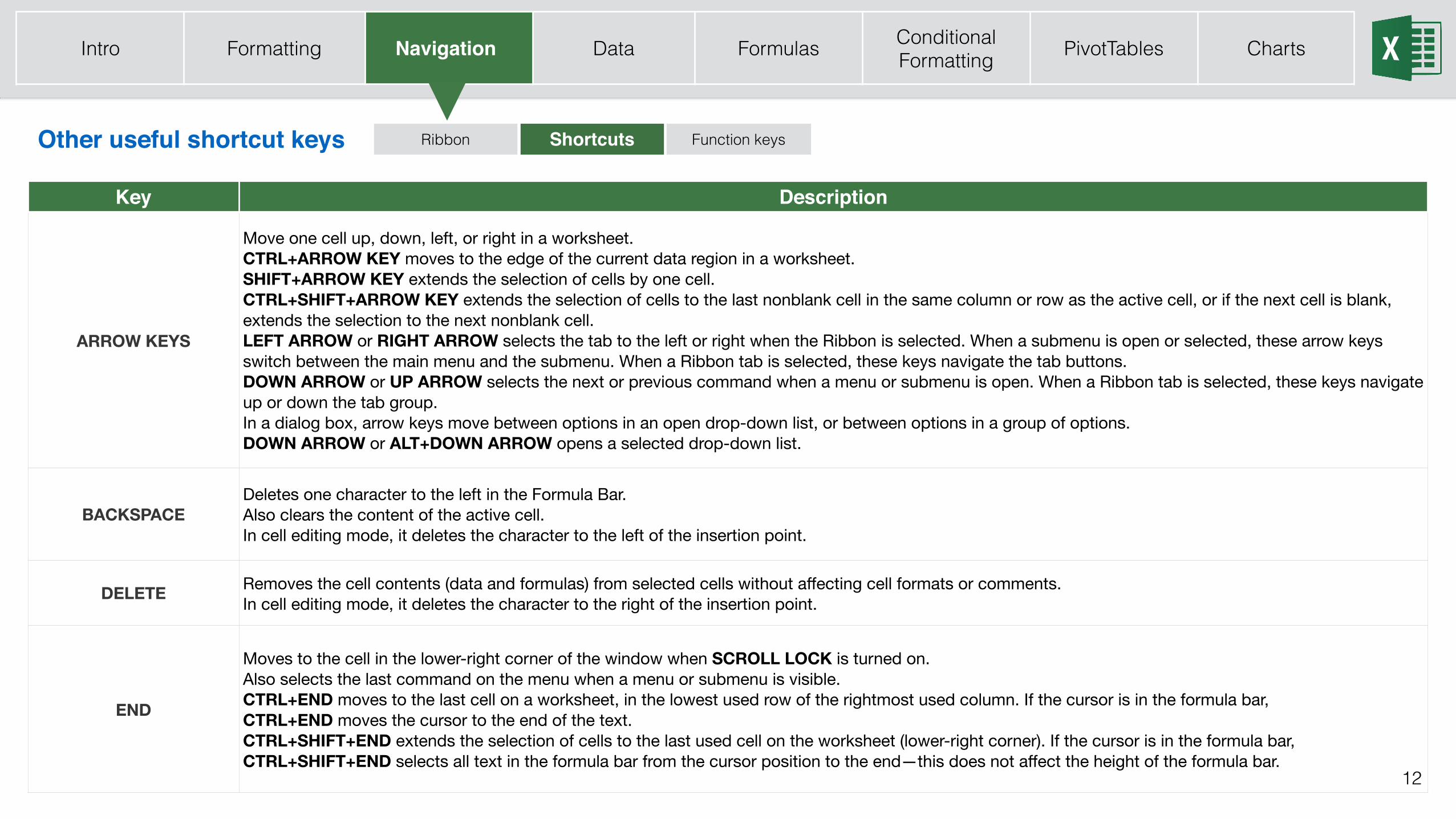
ARROW KEYS
Move one cell up, down, left, or right in a worksheet.CTRL+ARROW KEY moves to the edge of the current data region in a worksheet.SHIFT+ARROW KEY extends the selection of cells by one cell.CTRL+SHIFT+ARROW KEY extends the selection of cells to the last nonblank cell in the same column or row as the active cell, or if the next cell is blank, extends the selection to the next nonblank cell.LEFT ARROW or RIGHT ARROW selects the tab to the left or right when the Ribbon is selected. When a submenu is open or selected, these arrow keys switch between the main menu and the submenu. When a Ribbon tab is selected, these keys navigate the tab buttons.DOWN ARROW or UP ARROW selects the next or previous command when a menu or submenu is open. When a Ribbon tab is selected, these keys navigate up or down the tab group.In a dialog box, arrow keys move between options in an open drop-down list, or between options in a group of options.DOWN ARROW or ALT+DOWN ARROW opens a selected drop-down list.
BACKSPACEDeletes one character to the left in the Formula Bar.Also clears the content of the active cell.In cell editing mode, it deletes the character to the left of the insertion point.
DELETE Removes the cell contents (data and formulas) from selected cells without affecting cell formats or comments.In cell editing mode, it deletes the character to the right of the insertion point.
END
Moves to the cell in the lower-right corner of the window when SCROLL LOCK is turned on.Also selects the last command on the menu when a menu or submenu is visible.CTRL+END moves to the last cell on a worksheet, in the lowest used row of the rightmost used column. If the cursor is in the formula bar, CTRL+END moves the cursor to the end of the text.CTRL+SHIFT+END extends the selection of cells to the last used cell on the worksheet (lower-right corner). If the cursor is in the formula bar, CTRL+SHIFT+END selects all text in the formula bar from the cursor position to the end—this does not affect the height of the formula bar.
Other useful shortcut keys
Intro Formatting Navigation Data Formulas Conditional Formatting PivotTables Charts
13
Ribbon Shortcuts Function keys
Key Description
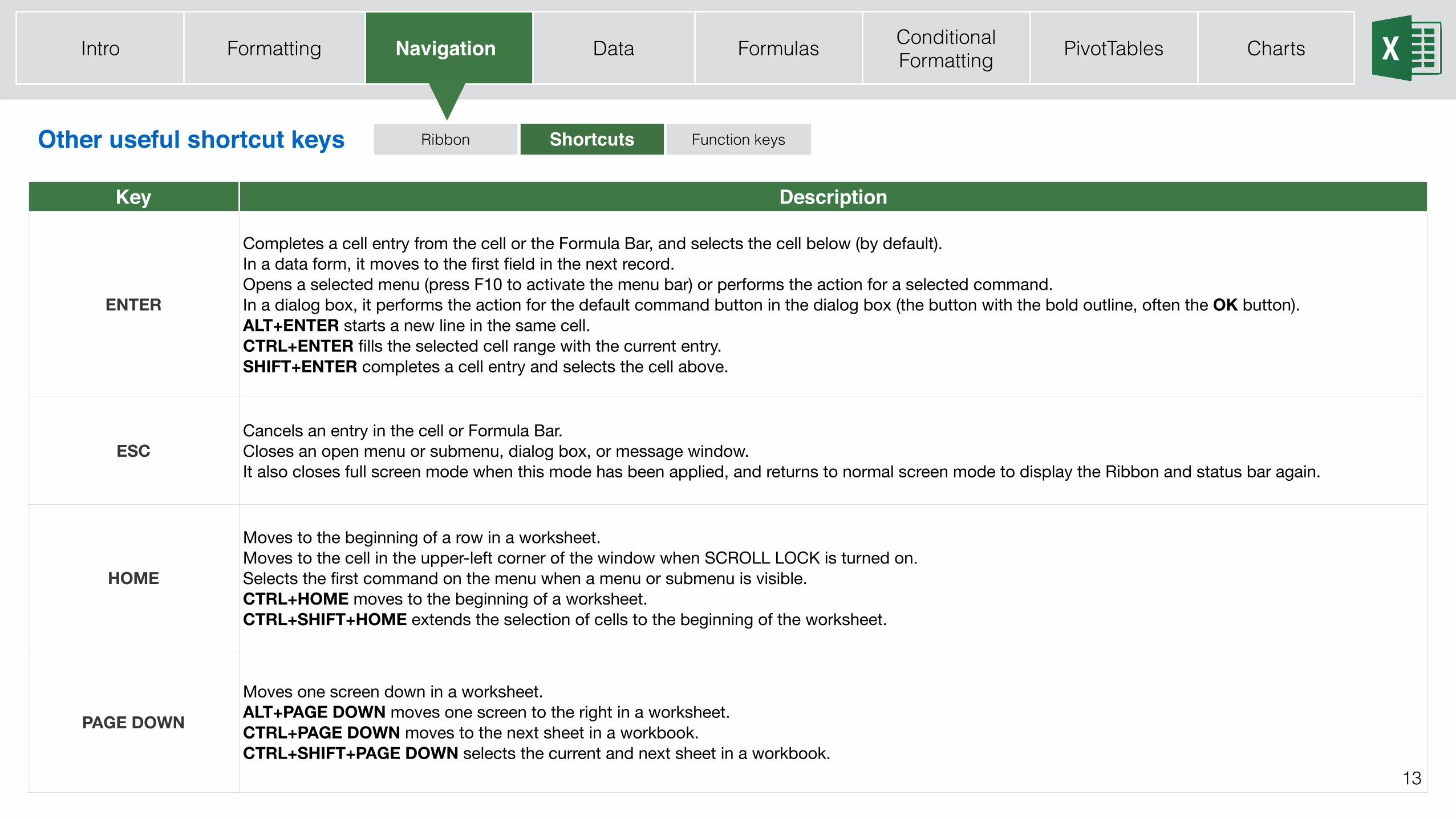
ENTER
Completes a cell entry from the cell or the Formula Bar, and selects the cell below (by default).In a data form, it moves to the first field in the next record.Opens a selected menu (press F10 to activate the menu bar) or performs the action for a selected command.In a dialog box, it performs the action for the default command button in the dialog box (the button with the bold outline, often the OK button).ALT+ENTER starts a new line in the same cell.CTRL+ENTER fills the selected cell range with the current entry.SHIFT+ENTER completes a cell entry and selects the cell above.
ESCCancels an entry in the cell or Formula Bar.Closes an open menu or submenu, dialog box, or message window.It also closes full screen mode when this mode has been applied, and returns to normal screen mode to display the Ribbon and status bar again.
HOME
Moves to the beginning of a row in a worksheet.Moves to the cell in the upper-left corner of the window when SCROLL LOCK is turned on.Selects the first command on the menu when a menu or submenu is visible.CTRL+HOME moves to the beginning of a worksheet.CTRL+SHIFT+HOME extends the selection of cells to the beginning of the worksheet.
PAGE DOWN
Moves one screen down in a worksheet.ALT+PAGE DOWN moves one screen to the right in a worksheet.CTRL+PAGE DOWN moves to the next sheet in a workbook.CTRL+SHIFT+PAGE DOWN selects the current and next sheet in a workbook.
Shortcuts Function keysOther useful shortcut keys
Intro Formatting Navigation Data Formulas Conditional Formatting PivotTables Charts
14
Ribbon Shortcuts Function keys
Key Description
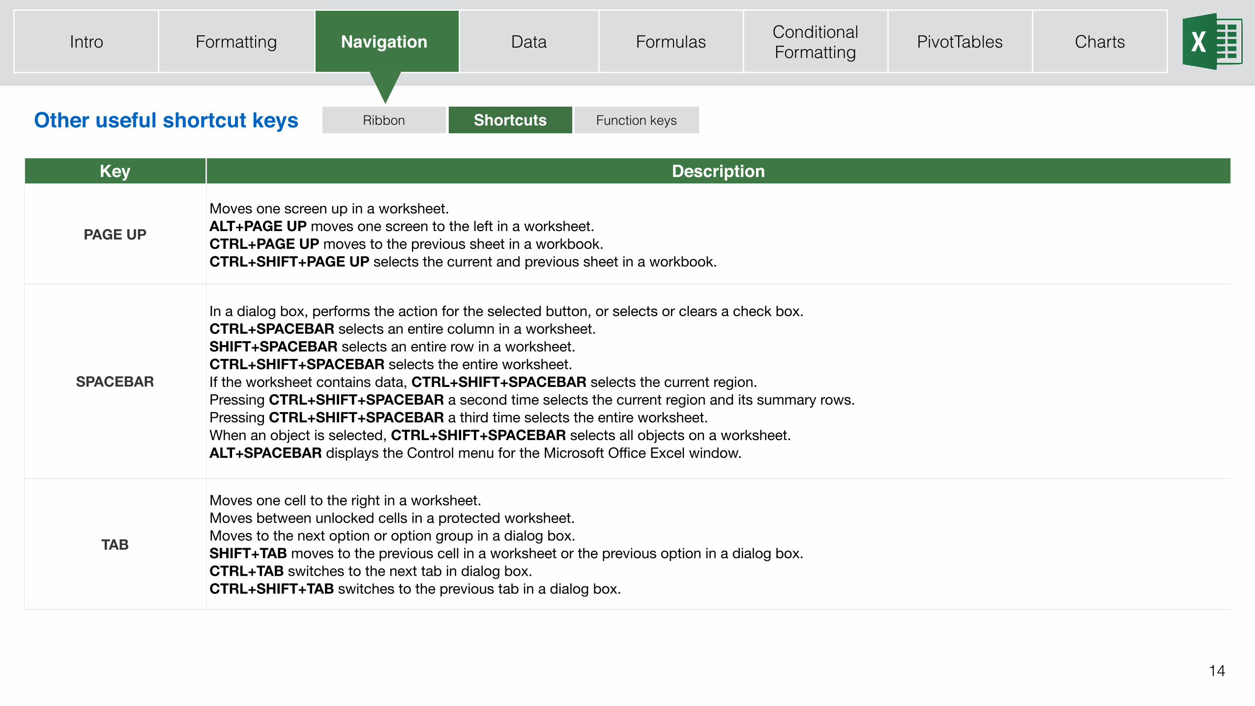
PAGE UP
Moves one screen up in a worksheet.ALT+PAGE UP moves one screen to the left in a worksheet.CTRL+PAGE UP moves to the previous sheet in a workbook.CTRL+SHIFT+PAGE UP selects the current and previous sheet in a workbook.
SPACEBAR
In a dialog box, performs the action for the selected button, or selects or clears a check box.CTRL+SPACEBAR selects an entire column in a worksheet.SHIFT+SPACEBAR selects an entire row in a worksheet.CTRL+SHIFT+SPACEBAR selects the entire worksheet. If the worksheet contains data, CTRL+SHIFT+SPACEBAR selects the current region. Pressing CTRL+SHIFT+SPACEBAR a second time selects the current region and its summary rows. Pressing CTRL+SHIFT+SPACEBAR a third time selects the entire worksheet. When an object is selected, CTRL+SHIFT+SPACEBAR selects all objects on a worksheet. ALT+SPACEBAR displays the Control menu for the Microsoft Office Excel window.
TAB
Moves one cell to the right in a worksheet.Moves between unlocked cells in a protected worksheet.Moves to the next option or option group in a dialog box.SHIFT+TAB moves to the previous cell in a worksheet or the previous option in a dialog box.CTRL+TAB switches to the next tab in dialog box.CTRL+SHIFT+TAB switches to the previous tab in a dialog box.
Shortcuts Function keysOther useful shortcut keys
Intro Formatting Navigation Data Formulas Conditional Formatting PivotTables Charts
15
Ribbon Shortcuts Function keys
Key Description
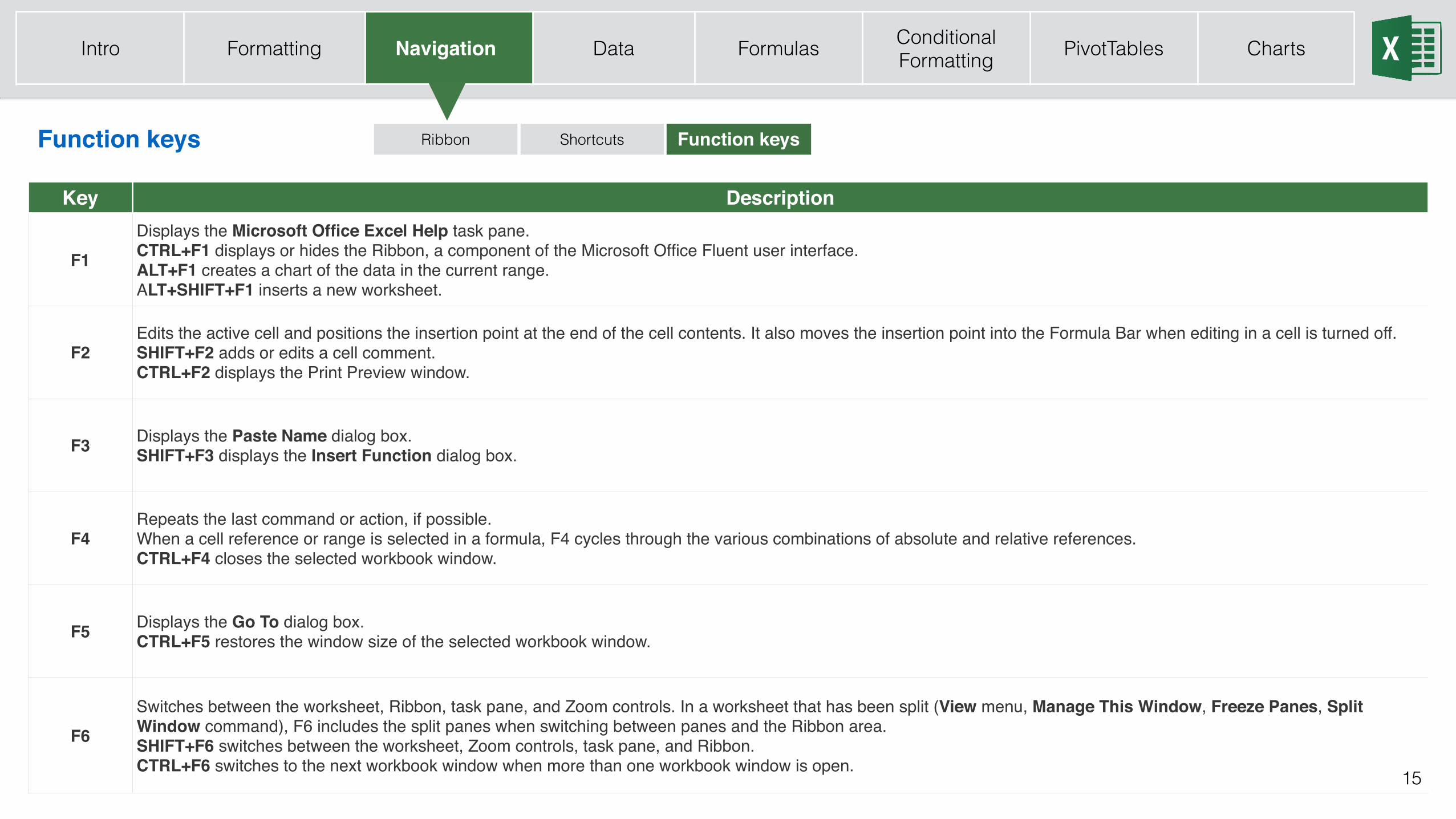
F1Displays the Microsoft Office Excel Help task pane.CTRL+F1 displays or hides the Ribbon, a component of the Microsoft Office Fluent user interface.ALT+F1 creates a chart of the data in the current range.ALT+SHIFT+F1 inserts a new worksheet.
F2Edits the active cell and positions the insertion point at the end of the cell contents. It also moves the insertion point into the Formula Bar when editing in a cell is turned off.SHIFT+F2 adds or edits a cell comment.CTRL+F2 displays the Print Preview window.
F3 Displays the Paste Name dialog box.SHIFT+F3 displays the Insert Function dialog box.
F4Repeats the last command or action, if possible.When a cell reference or range is selected in a formula, F4 cycles through the various combinations of absolute and relative references.CTRL+F4 closes the selected workbook window.
F5 Displays the Go To dialog box.CTRL+F5 restores the window size of the selected workbook window.
F6Switches between the worksheet, Ribbon, task pane, and Zoom controls. In a worksheet that has been split (View menu, Manage This Window, Freeze Panes, Split Window command), F6 includes the split panes when switching between panes and the Ribbon area.SHIFT+F6 switches between the worksheet, Zoom controls, task pane, and Ribbon.CTRL+F6 switches to the next workbook window when more than one workbook window is open.
Function keys
Intro Formatting Navigation Data Formulas Conditional Formatting PivotTables Charts
16
Ribbon Shortcuts Function keys
Key Description
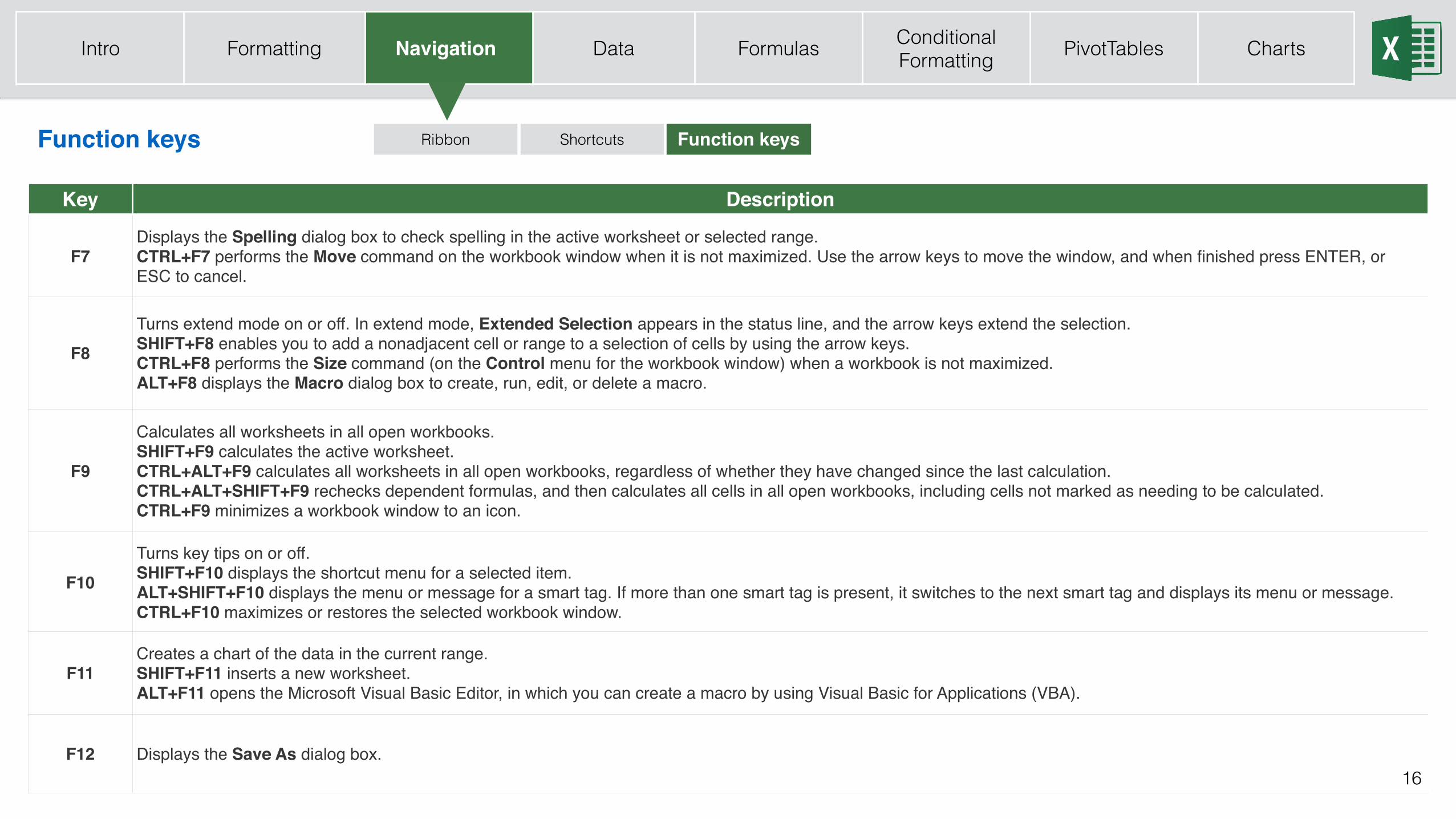
F7Displays the Spelling dialog box to check spelling in the active worksheet or selected range.CTRL+F7 performs the Move command on the workbook window when it is not maximized. Use the arrow keys to move the window, and when finished press ENTER, or ESC to cancel.
F8Turns extend mode on or off. In extend mode, Extended Selection appears in the status line, and the arrow keys extend the selection.SHIFT+F8 enables you to add a nonadjacent cell or range to a selection of cells by using the arrow keys.CTRL+F8 performs the Size command (on the Control menu for the workbook window) when a workbook is not maximized.ALT+F8 displays the Macro dialog box to create, run, edit, or delete a macro.
F9
Calculates all worksheets in all open workbooks.SHIFT+F9 calculates the active worksheet.CTRL+ALT+F9 calculates all worksheets in all open workbooks, regardless of whether they have changed since the last calculation.CTRL+ALT+SHIFT+F9 rechecks dependent formulas, and then calculates all cells in all open workbooks, including cells not marked as needing to be calculated.CTRL+F9 minimizes a workbook window to an icon.
F10Turns key tips on or off.SHIFT+F10 displays the shortcut menu for a selected item.ALT+SHIFT+F10 displays the menu or message for a smart tag. If more than one smart tag is present, it switches to the next smart tag and displays its menu or message.CTRL+F10 maximizes or restores the selected workbook window.
F11Creates a chart of the data in the current range.SHIFT+F11 inserts a new worksheet.ALT+F11 opens the Microsoft Visual Basic Editor, in which you can create a macro by using Visual Basic for Applications (VBA).
F12 Displays the Save As dialog box.
Function keys
Intro Formatting Navigation Data Formulas Conditional Formatting PivotTables Charts
17
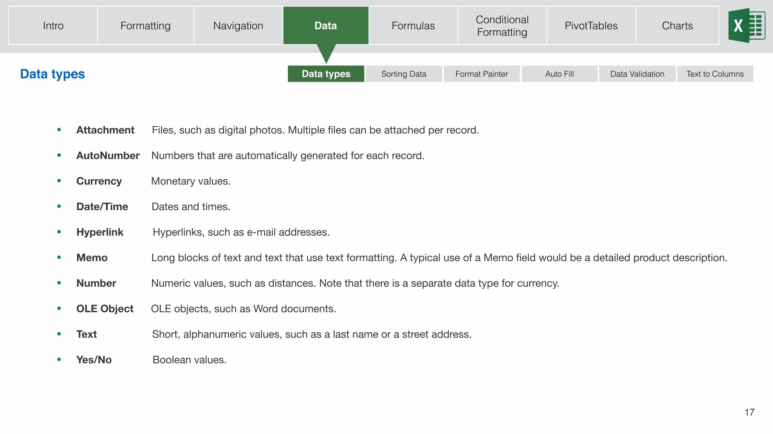
• Attachment Files, such as digital photos. Multiple files can be attached per record.
• AutoNumber Numbers that are automatically generated for each record.
• Currency Monetary values.
• Date/Time Dates and times.
• Hyperlink Hyperlinks, such as e-mail addresses.
• Memo Long blocks of text and text that use text formatting. A typical use of a Memo field would be a detailed product description.
• Number Numeric values, such as distances. Note that there is a separate data type for currency.
• OLE Object OLE objects, such as Word documents.
• Text Short, alphanumeric values, such as a last name or a street address.
• Yes/No Boolean values.
Data types Data types Sorting Data Auto Fill Data Validation Text to ColumnsFormat Painter
Intro Formatting Navigation Data Formulas Conditional Formatting PivotTables Charts
18
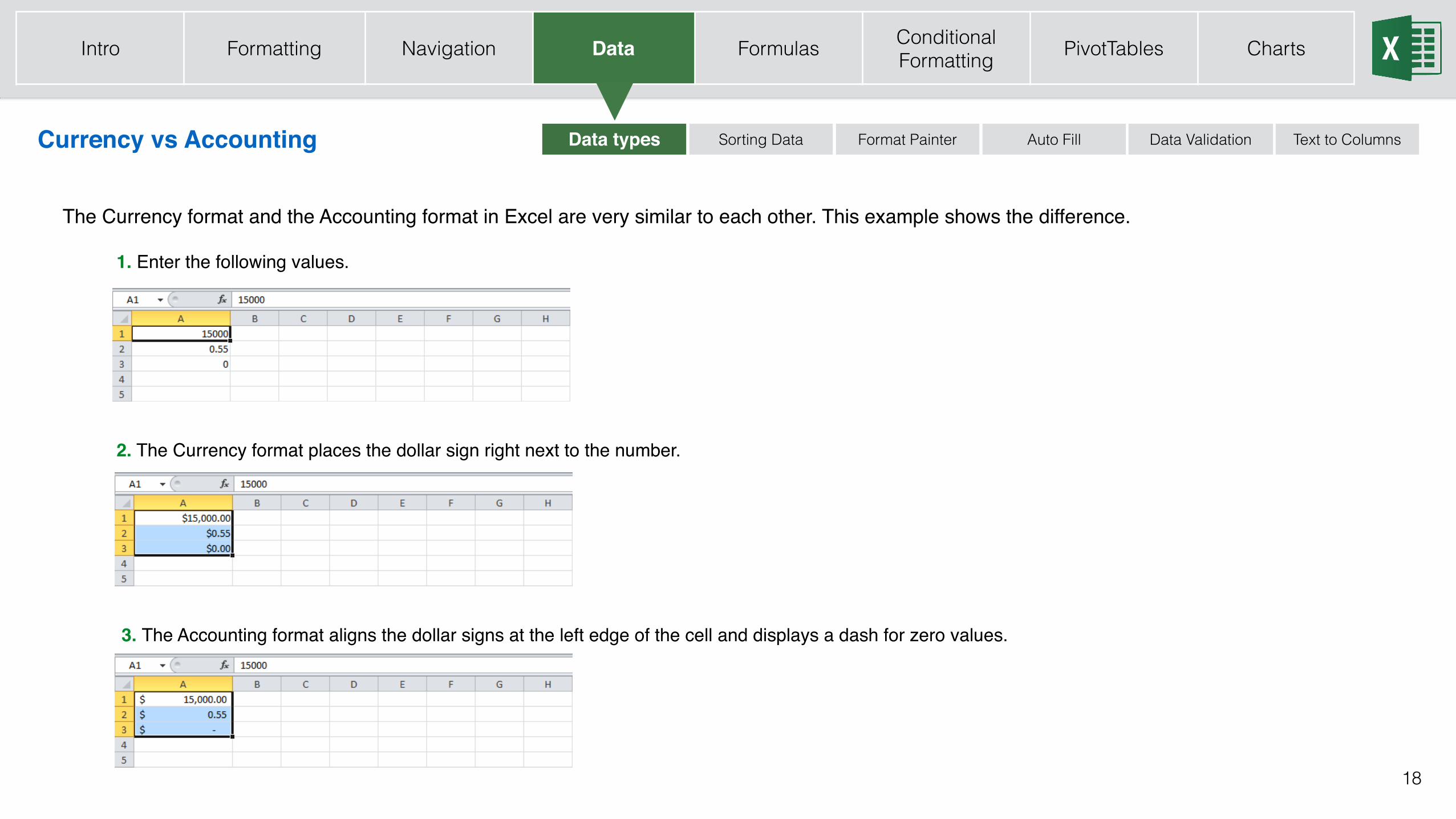
The Currency format and the Accounting format in Excel are very similar to each other. This example shows the difference.
2. The Currency format places the dollar sign right next to the number.
3. The Accounting format aligns the dollar signs at the left edge of the cell and displays a dash for zero values.
1. Enter the following values.
Currency vs Accounting Data types Sorting Data Auto Fill Data Validation Text to ColumnsFormat Painter
Intro Formatting Navigation Data Formulas Conditional Formatting PivotTables Charts
19
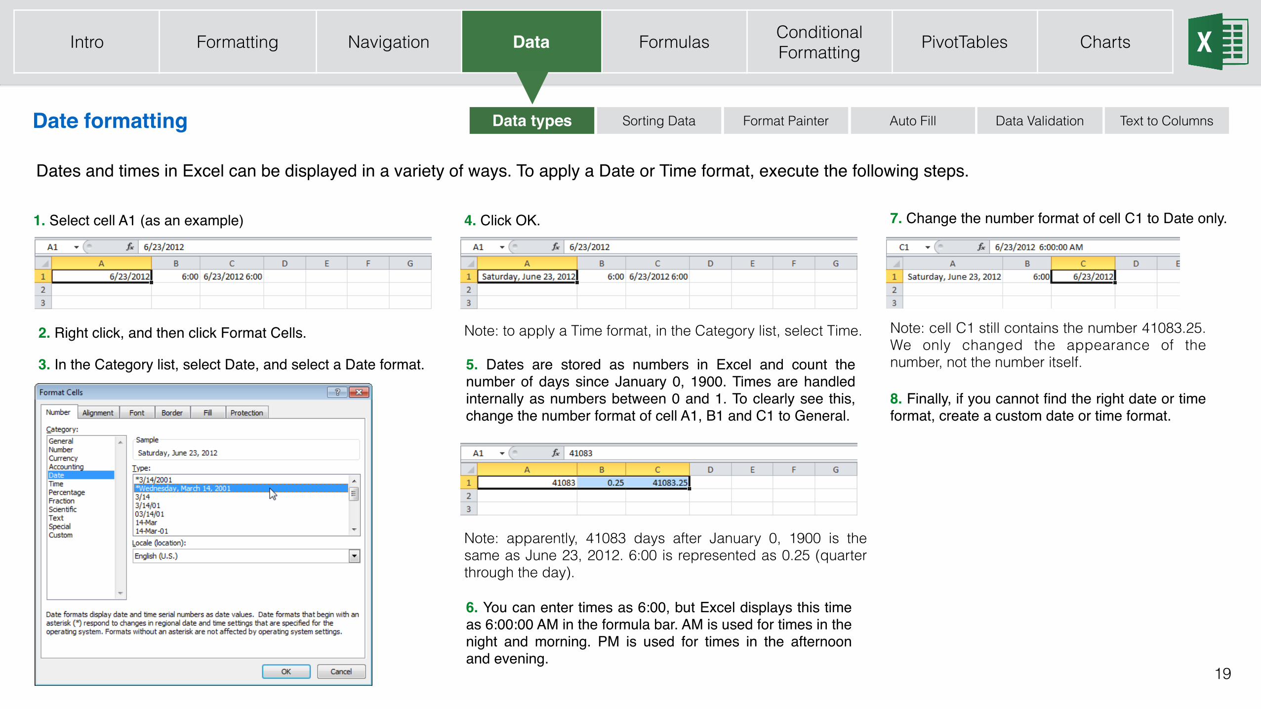
Dates and times in Excel can be displayed in a variety of ways. To apply a Date or Time format, execute the following steps.
2. Right click, and then click Format Cells.
3. In the Category list, select Date, and select a Date format.
1. Select cell A1 (as an example) 4. Click OK.
Note: to apply a Time format, in the Category list, select Time.
Note: apparently, 41083 days after January 0, 1900 is the same as June 23, 2012. 6:00 is represented as 0.25 (quarter through the day).
5. Dates are stored as numbers in Excel and count the number of days since January 0, 1900. Times are handled internally as numbers between 0 and 1. To clearly see this, change the number format of cell A1, B1 and C1 to General.
6. You can enter times as 6:00, but Excel displays this time as 6:00:00 AM in the formula bar. AM is used for times in the night and morning. PM is used for times in the afternoon and evening.
7. Change the number format of cell C1 to Date only.
Note: cell C1 still contains the number 41083.25. We only changed the appearance of the number, not the number itself.
8. Finally, if you cannot find the right date or time format, create a custom date or time format.
Date formatting Data types Sorting Data Auto Fill Data Validation Text to ColumnsFormat Painter
Intro Formatting Navigation Data Formulas Conditional Formatting PivotTables Charts
20
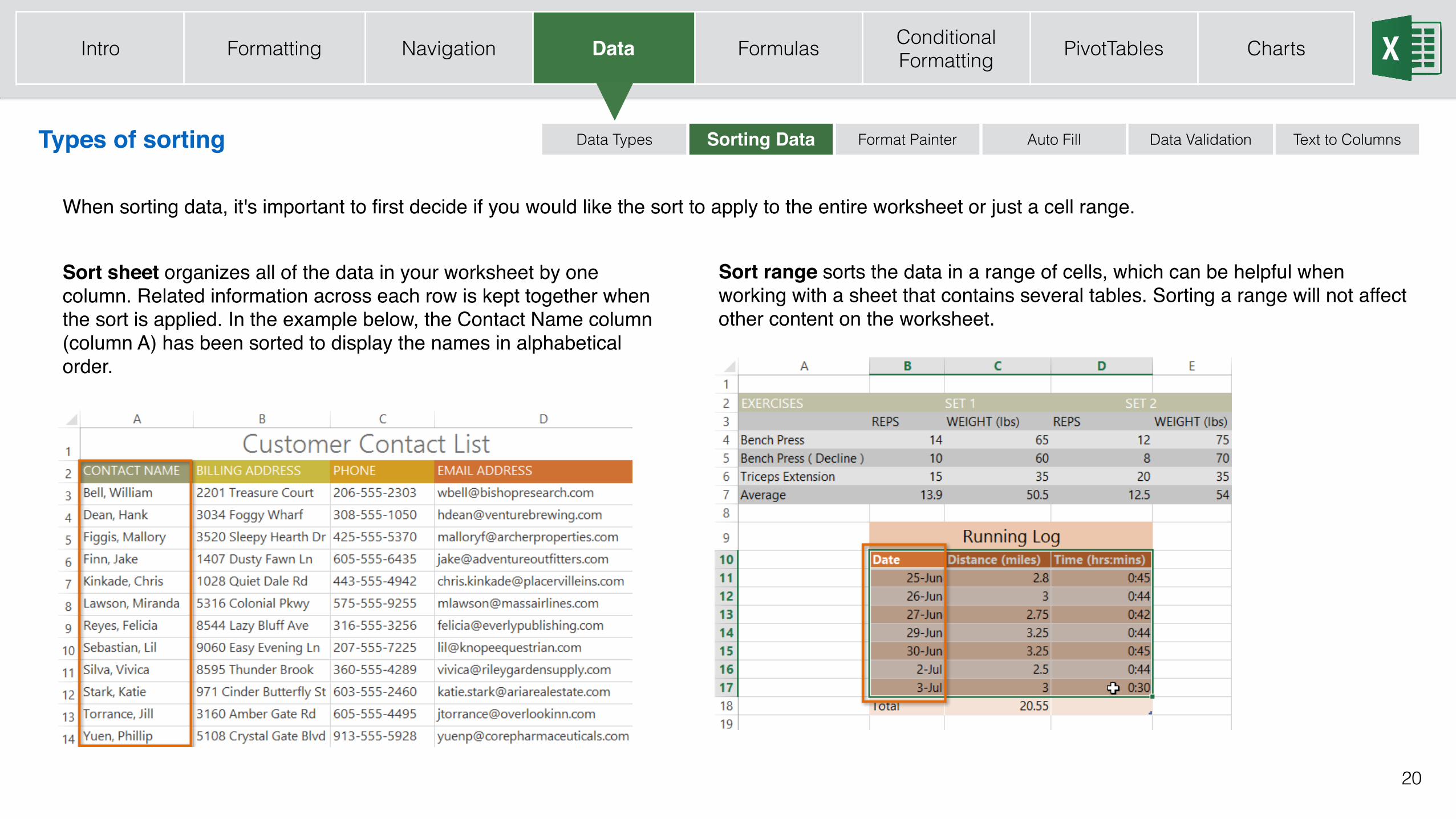
When sorting data, it's important to first decide if you would like the sort to apply to the entire worksheet or just a cell range.
Types of sorting Auto Fill Data ValidationSorting Data Text to ColumnsFormat PainterData Types
Intro Formatting Navigation Data Formulas Conditional Formatting PivotTables Charts
Sort range sorts the data in a range of cells, which can be helpful when working with a sheet that contains several tables. Sorting a range will not affect other content on the worksheet.
Sort sheet organizes all of the data in your worksheet by one column. Related information across each row is kept together when the sort is applied. In the example below, the Contact Name column (column A) has been sorted to display the names in alphabetical order.
21
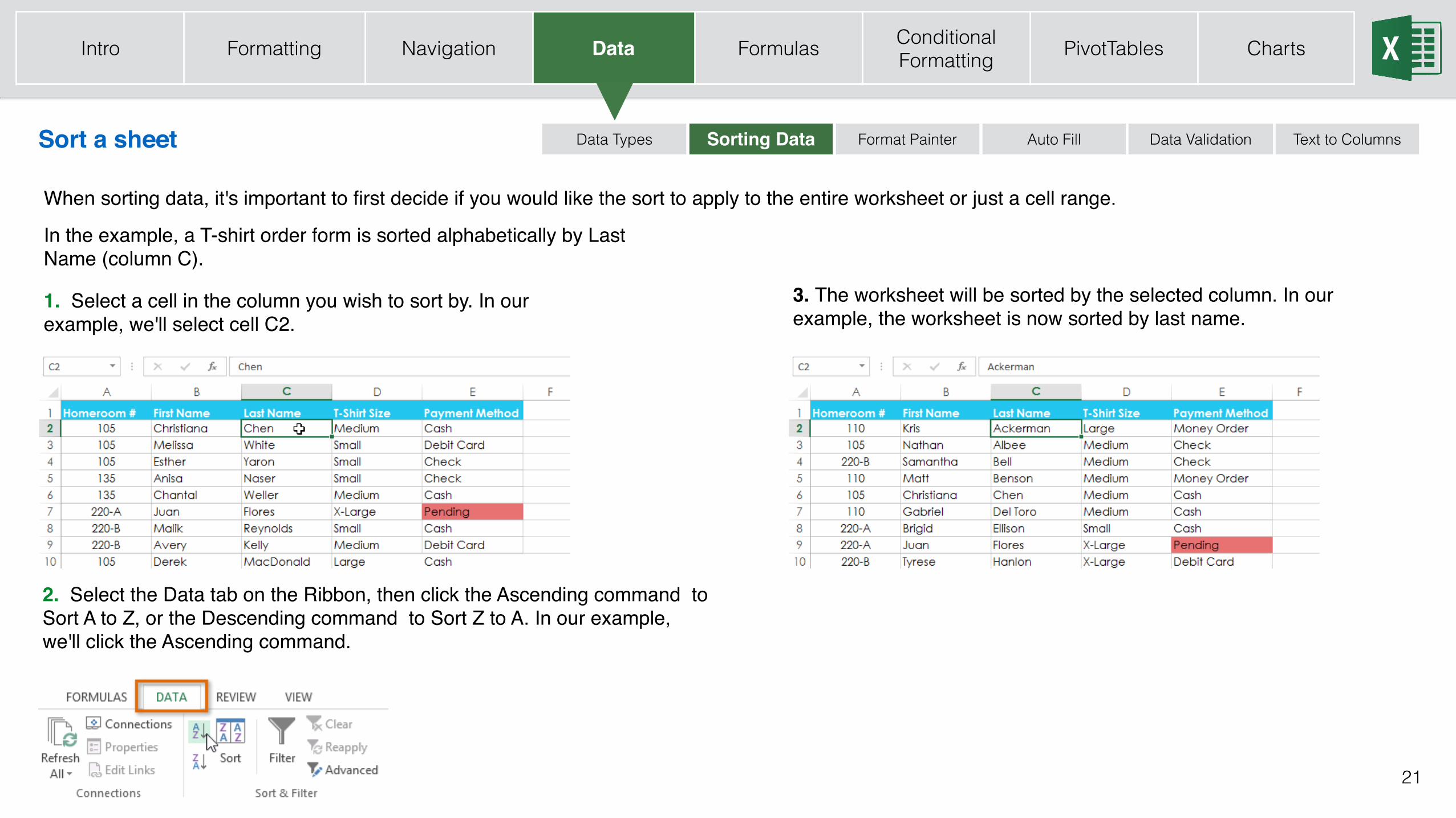
When sorting data, it's important to first decide if you would like the sort to apply to the entire worksheet or just a cell range.
Sort a sheet Auto Fill Data ValidationSorting Data Text to ColumnsFormat PainterData Types
Intro Formatting Navigation Data Formulas Conditional Formatting PivotTables Charts
In the example, a T-shirt order form is sorted alphabetically by Last Name (column C).
1. Select a cell in the column you wish to sort by. In our example, we'll select cell C2.
2. Select the Data tab on the Ribbon, then click the Ascending command to Sort A to Z, or the Descending command to Sort Z to A. In our example, we'll click the Ascending command.
3. The worksheet will be sorted by the selected column. In our example, the worksheet is now sorted by last name.
22
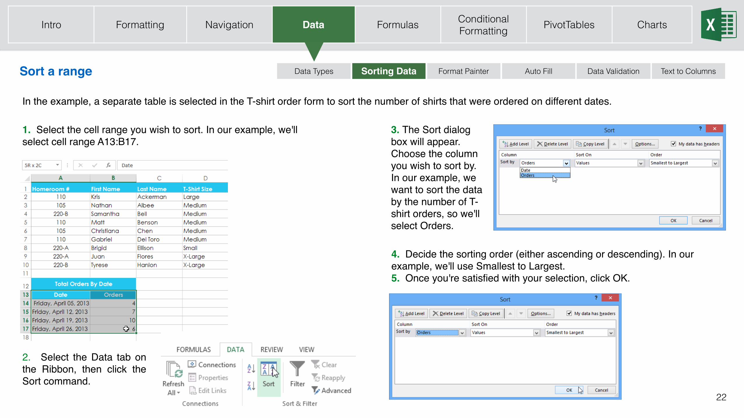
In the example, a separate table is selected in the T-shirt order form to sort the number of shirts that were ordered on different dates.
Sort a range Auto Fill Data ValidationSorting Data Text to ColumnsFormat PainterData Types
Intro Formatting Navigation Data Formulas Conditional Formatting PivotTables Charts
3. The Sort dialog box will appear. Choose the column you wish to sort by. In our example, we want to sort the data by the number of T-shirt orders, so we'll select Orders.
1. Select the cell range you wish to sort. In our example, we'll select cell range A13:B17.
2. Select the Data tab on the Ribbon, then click the Sort command.
4. Decide the sorting order (either ascending or descending). In our example, we'll use Smallest to Largest.5. Once you're satisfied with your selection, click OK.
23
Sort a range Auto Fill Data ValidationSorting Data Text to ColumnsFormat PainterData Types
Intro Formatting Navigation Data Formulas Conditional Formatting PivotTables Charts
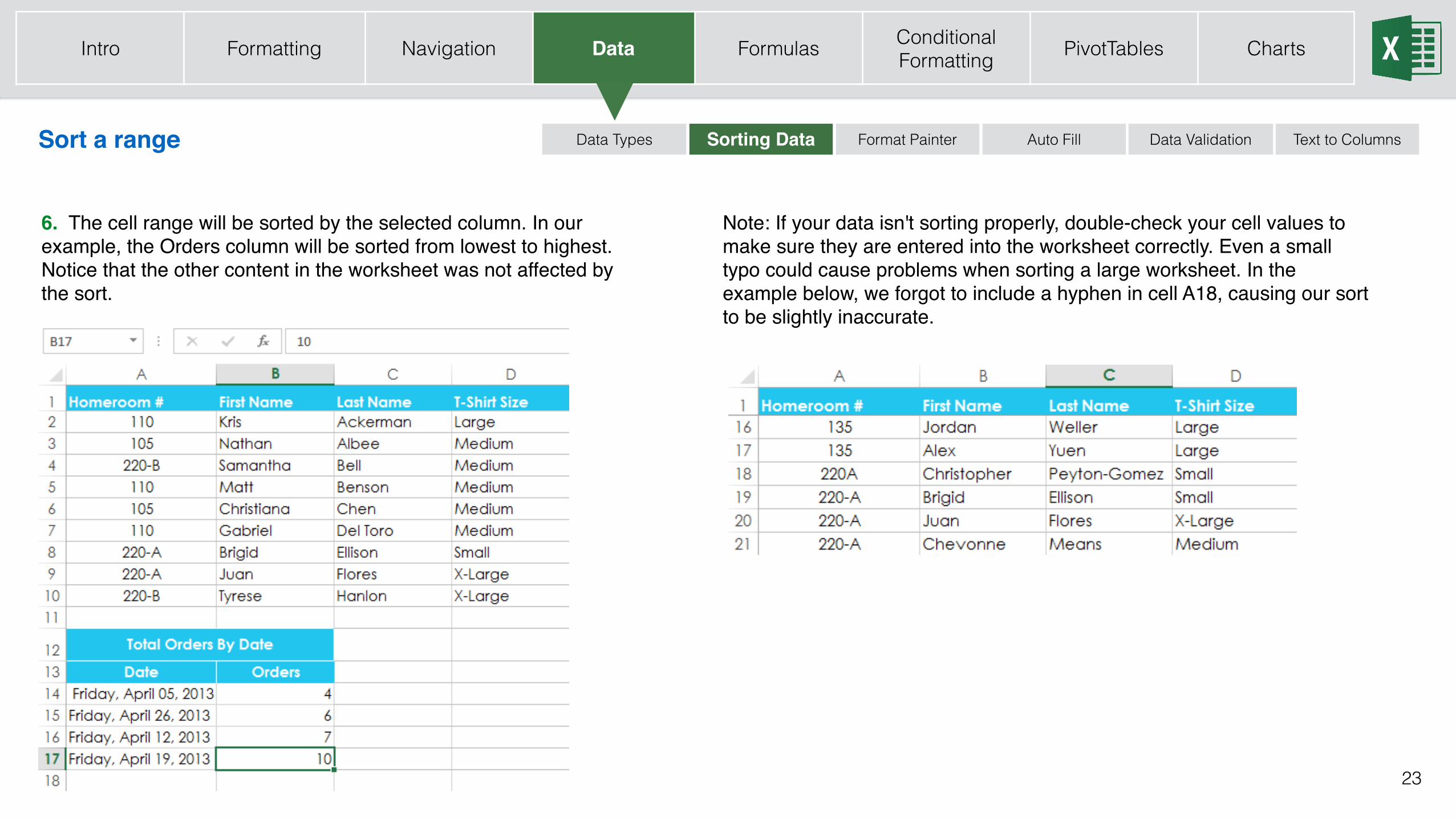
6. The cell range will be sorted by the selected column. In our example, the Orders column will be sorted from lowest to highest. Notice that the other content in the worksheet was not affected by the sort.
Note: If your data isn't sorting properly, double-check your cell values to make sure they are entered into the worksheet correctly. Even a small typo could cause problems when sorting a large worksheet. In the example below, we forgot to include a hyphen in cell A18, causing our sort to be slightly inaccurate.
24
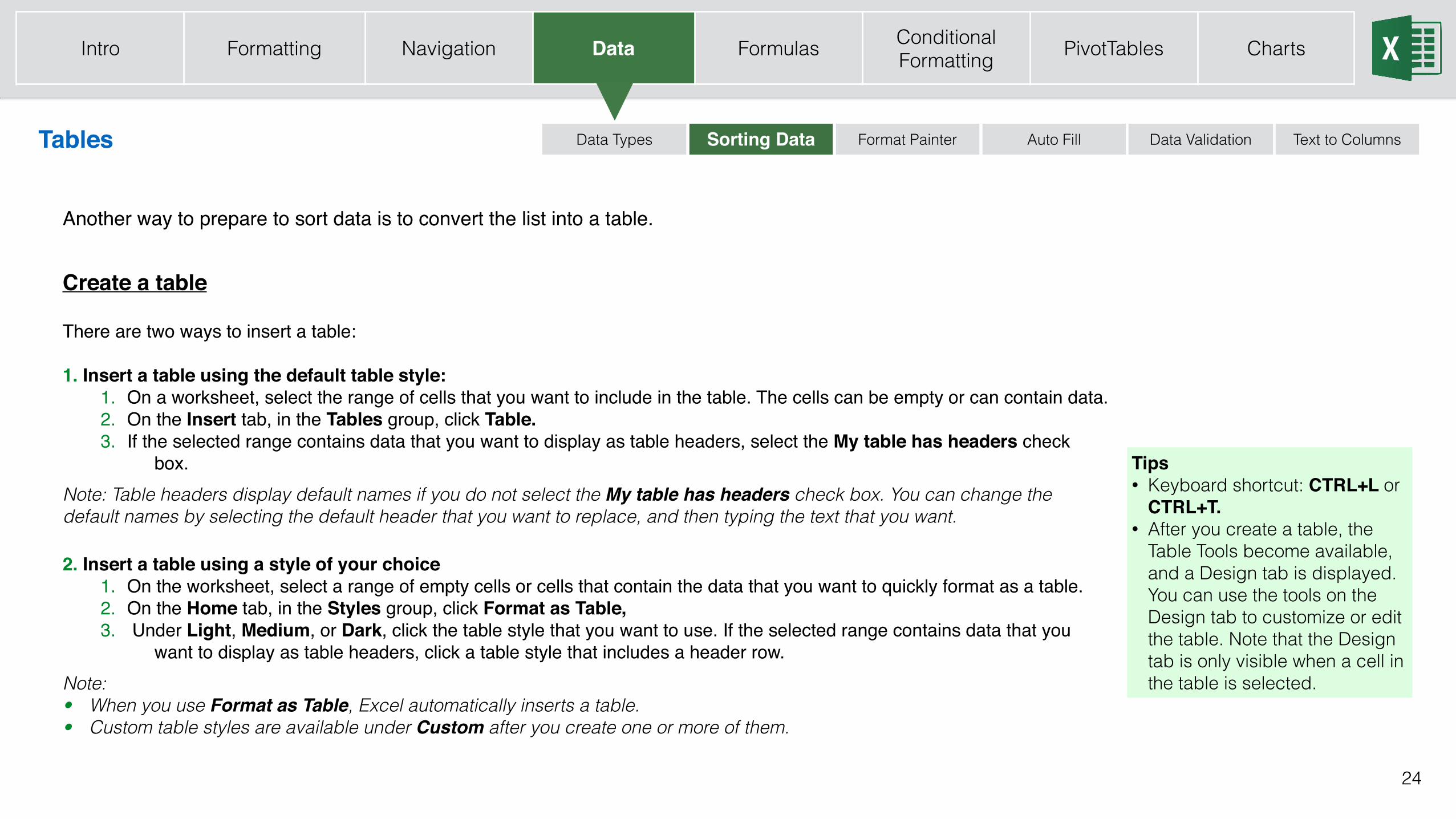
Another way to prepare to sort data is to convert the list into a table.
Create a table
There are two ways to insert a table:
1. Insert a table using the default table style:1. On a worksheet, select the range of cells that you want to include in the table. The cells can be empty or can contain data.2. On the Insert tab, in the Tables group, click Table.3. If the selected range contains data that you want to display as table headers, select the My table has headers check
box. Note: Table headers display default names if you do not select the My table has headers check box. You can change the default names by selecting the default header that you want to replace, and then typing the text that you want.
2. Insert a table using a style of your choice1. On the worksheet, select a range of empty cells or cells that contain the data that you want to quickly format as a table.2. On the Home tab, in the Styles group, click Format as Table,3. Under Light, Medium, or Dark, click the table style that you want to use. If the selected range contains data that you
want to display as table headers, click a table style that includes a header row.Note: • When you use Format as Table, Excel automatically inserts a table. • Custom table styles are available under Custom after you create one or more of them.
Tips• Keyboard shortcut: CTRL+L or
CTRL+T. • After you create a table, the
Table Tools become available, and a Design tab is displayed. You can use the tools on the Design tab to customize or edit the table. Note that the Design tab is only visible when a cell in the table is selected.
Tables Auto Fill Data ValidationSorting Data Text to ColumnsFormat PainterData Types
Intro Formatting Navigation Data Formulas Conditional Formatting PivotTables Charts
25
Auto Fill Data ValidationSorting Data Text to ColumnsFormat PainterData Types
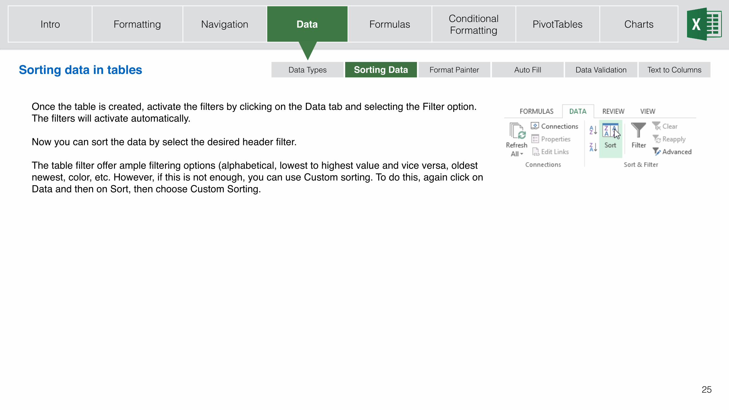
Once the table is created, activate the filters by clicking on the Data tab and selecting the Filter option.The filters will activate automatically.
Now you can sort the data by select the desired header filter.
The table filter offer ample filtering options (alphabetical, lowest to highest value and vice versa, oldest newest, color, etc. However, if this is not enough, you can use Custom sorting. To do this, again click on Data and then on Sort, then choose Custom Sorting.
Sorting data in tables
Intro Formatting Navigation Data Formulas Conditional Formatting PivotTables Charts
26
Auto Fill Data ValidationSorting Data Text to ColumnsFormat PainterData TypesFormat Painter
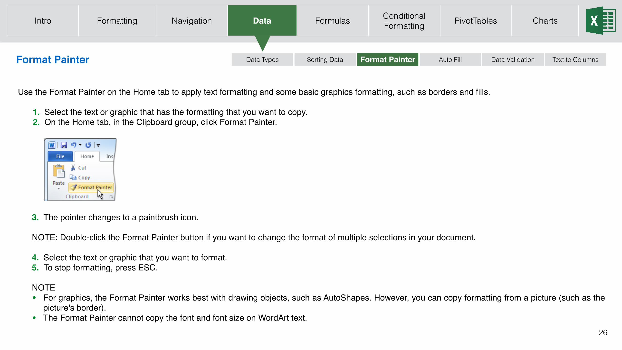
Use the Format Painter on the Home tab to apply text formatting and some basic graphics formatting, such as borders and fills.
1. Select the text or graphic that has the formatting that you want to copy.2. On the Home tab, in the Clipboard group, click Format Painter.
3. The pointer changes to a paintbrush icon.
NOTE: Double-click the Format Painter button if you want to change the format of multiple selections in your document.
4. Select the text or graphic that you want to format.5. To stop formatting, press ESC.
NOTE • For graphics, the Format Painter works best with drawing objects, such as AutoShapes. However, you can copy formatting from a picture (such as the
picture's border).• The Format Painter cannot copy the font and font size on WordArt text.
Intro Formatting Navigation Data Formulas Conditional Formatting PivotTables Charts
27
Auto Fill Data ValidationSorting Data Text to ColumnsFormat PainterData Types
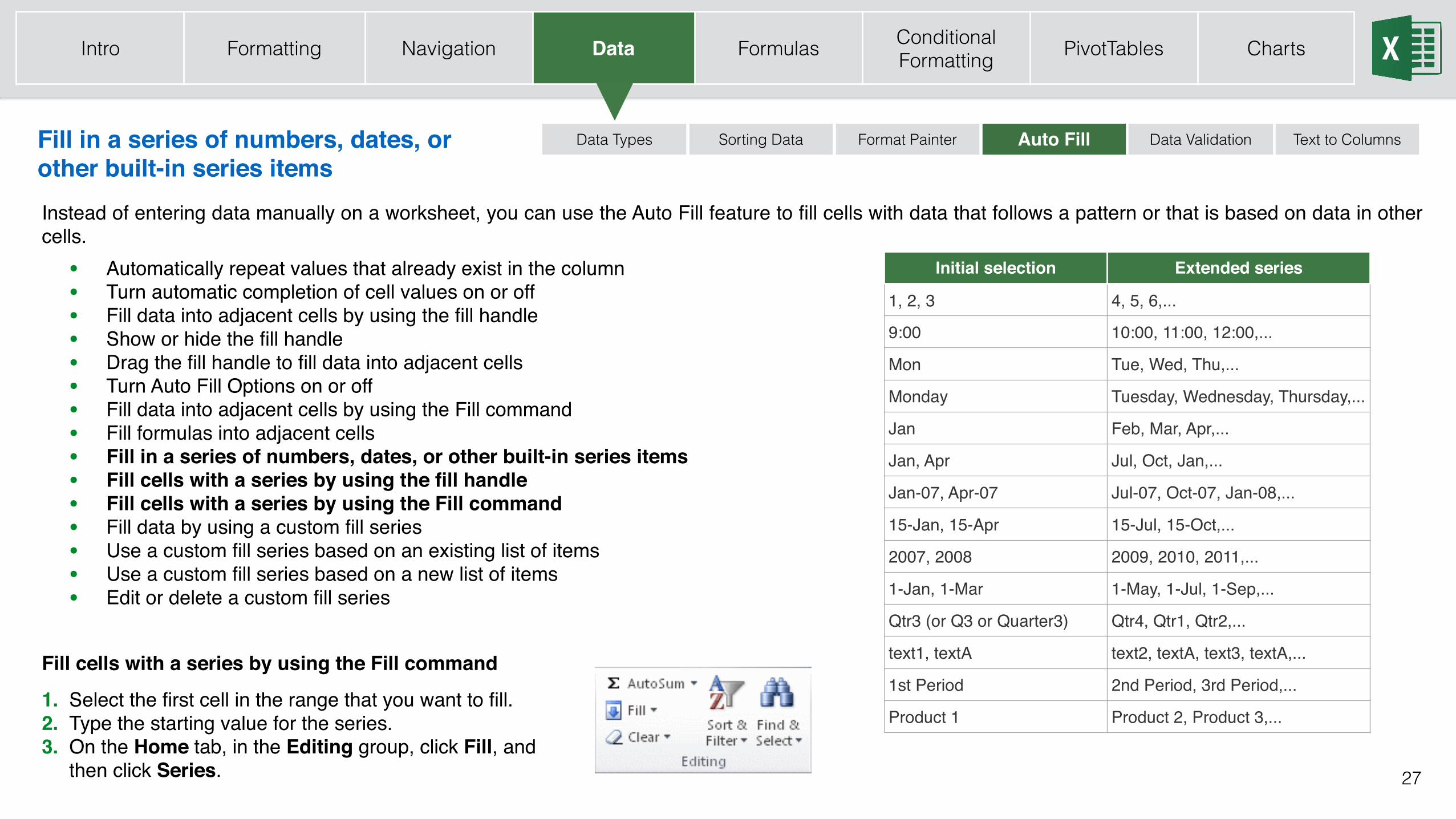
Instead of entering data manually on a worksheet, you can use the Auto Fill feature to fill cells with data that follows a pattern or that is based on data in other cells.
• Automatically repeat values that already exist in the column• Turn automatic completion of cell values on or off• Fill data into adjacent cells by using the fill handle• Show or hide the fill handle• Drag the fill handle to fill data into adjacent cells• Turn Auto Fill Options on or off• Fill data into adjacent cells by using the Fill command• Fill formulas into adjacent cells• Fill in a series of numbers, dates, or other built-in series items• Fill cells with a series by using the fill handle• Fill cells with a series by using the Fill command• Fill data by using a custom fill series• Use a custom fill series based on an existing list of items• Use a custom fill series based on a new list of items• Edit or delete a custom fill series
Fill cells with a series by using the Fill command
1. Select the first cell in the range that you want to fill.2. Type the starting value for the series.3. On the Home tab, in the Editing group, click Fill, and
then click Series.
Fill in a series of numbers, dates, or other built-in series items
Initial selection Extended series
1, 2, 3 4, 5, 6,...
9:00 10:00, 11:00, 12:00,...
Mon Tue, Wed, Thu,...
Monday Tuesday, Wednesday, Thursday,...
Jan Feb, Mar, Apr,...
Jan, Apr Jul, Oct, Jan,...
Jan-07, Apr-07 Jul-07, Oct-07, Jan-08,...
15-Jan, 15-Apr 15-Jul, 15-Oct,...
2007, 2008 2009, 2010, 2011,...
1-Jan, 1-Mar 1-May, 1-Jul, 1-Sep,...
Qtr3 (or Q3 or Quarter3) Qtr4, Qtr1, Qtr2,...
text1, textA text2, textA, text3, textA,...
1st Period 2nd Period, 3rd Period,...
Product 1 Product 2, Product 3,...
Intro Formatting Navigation Data Formulas Conditional Formatting PivotTables Charts
28
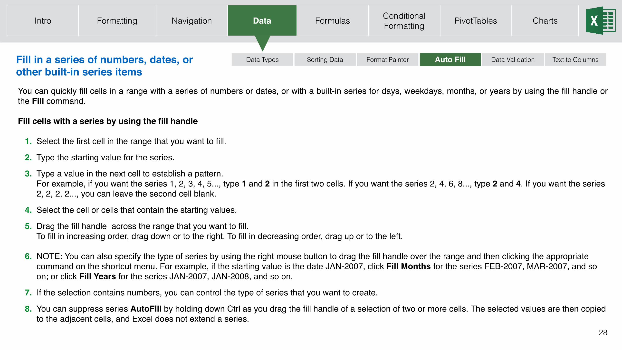
Auto Fill Data ValidationSorting Data Text to ColumnsFormat PainterData TypesFill in a series of numbers, dates, or other built-in series itemsYou can quickly fill cells in a range with a series of numbers or dates, or with a built-in series for days, weekdays, months, or years by using the fill handle or the Fill command.
Fill cells with a series by using the fill handle
1. Select the first cell in the range that you want to fill.
2. Type the starting value for the series.
3. Type a value in the next cell to establish a pattern. For example, if you want the series 1, 2, 3, 4, 5..., type 1 and 2 in the first two cells. If you want the series 2, 4, 6, 8..., type 2 and 4. If you want the series
2, 2, 2, 2..., you can leave the second cell blank.
4. Select the cell or cells that contain the starting values.
5. Drag the fill handle across the range that you want to fill. To fill in increasing order, drag down or to the right. To fill in decreasing order, drag up or to the left.
6. NOTE: You can also specify the type of series by using the right mouse button to drag the fill handle over the range and then clicking the appropriate command on the shortcut menu. For example, if the starting value is the date JAN-2007, click Fill Months for the series FEB-2007, MAR-2007, and so on; or click Fill Years for the series JAN-2007, JAN-2008, and so on.
7. If the selection contains numbers, you can control the type of series that you want to create.
8. You can suppress series AutoFill by holding down Ctrl as you drag the fill handle of a selection of two or more cells. The selected values are then copied to the adjacent cells, and Excel does not extend a series.
Intro Formatting Navigation Data Formulas Conditional Formatting PivotTables Charts
29
Auto Fill Data ValidationSorting Data Text to ColumnsFormat PainterData TypesData Validation Use
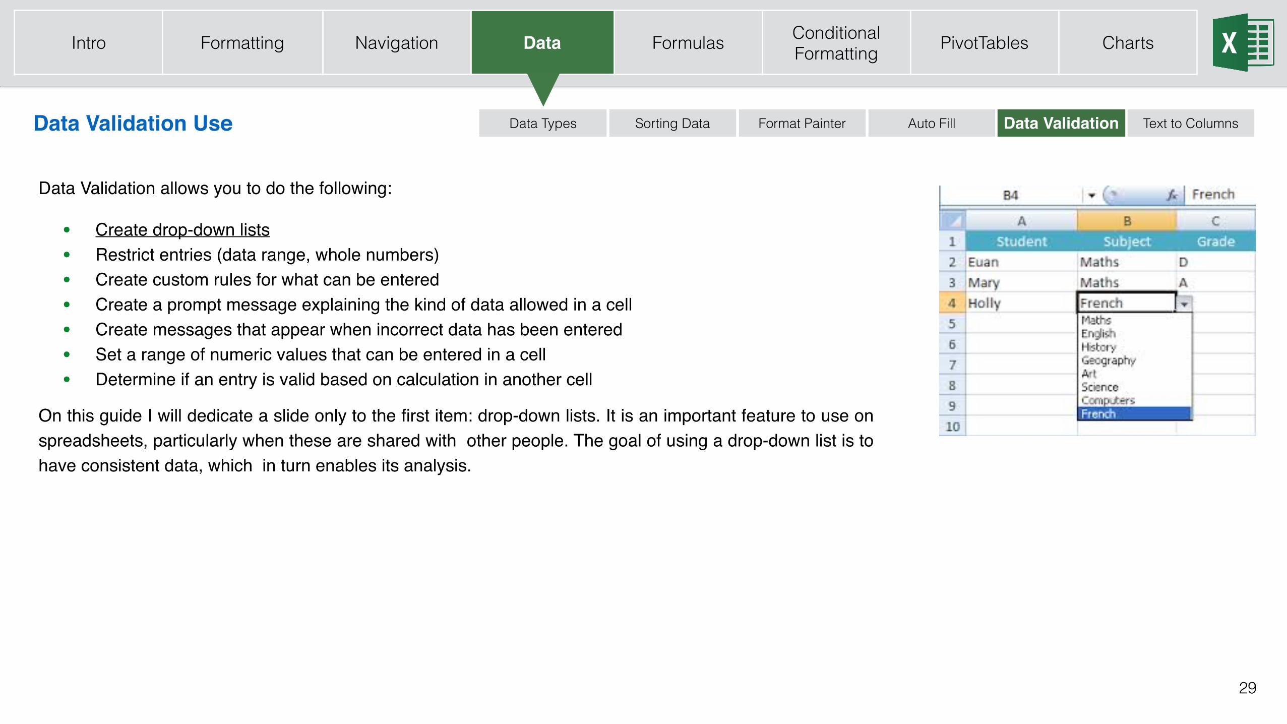
Data Validation allows you to do the following:
• Create drop-down lists• Restrict entries (data range, whole numbers)• Create custom rules for what can be entered• Create a prompt message explaining the kind of data allowed in a cell• Create messages that appear when incorrect data has been entered• Set a range of numeric values that can be entered in a cell• Determine if an entry is valid based on calculation in another cell
On this guide I will dedicate a slide only to the first item: drop-down lists. It is an important feature to use on spreadsheets, particularly when these are shared with other people. The goal of using a drop-down list is to have consistent data, which in turn enables its analysis.
Intro Formatting Navigation Data Formulas Conditional Formatting PivotTables Charts
30
Auto Fill Data ValidationSorting Data Text to ColumnsFormat PainterData TypesCreate a Drop-Down List
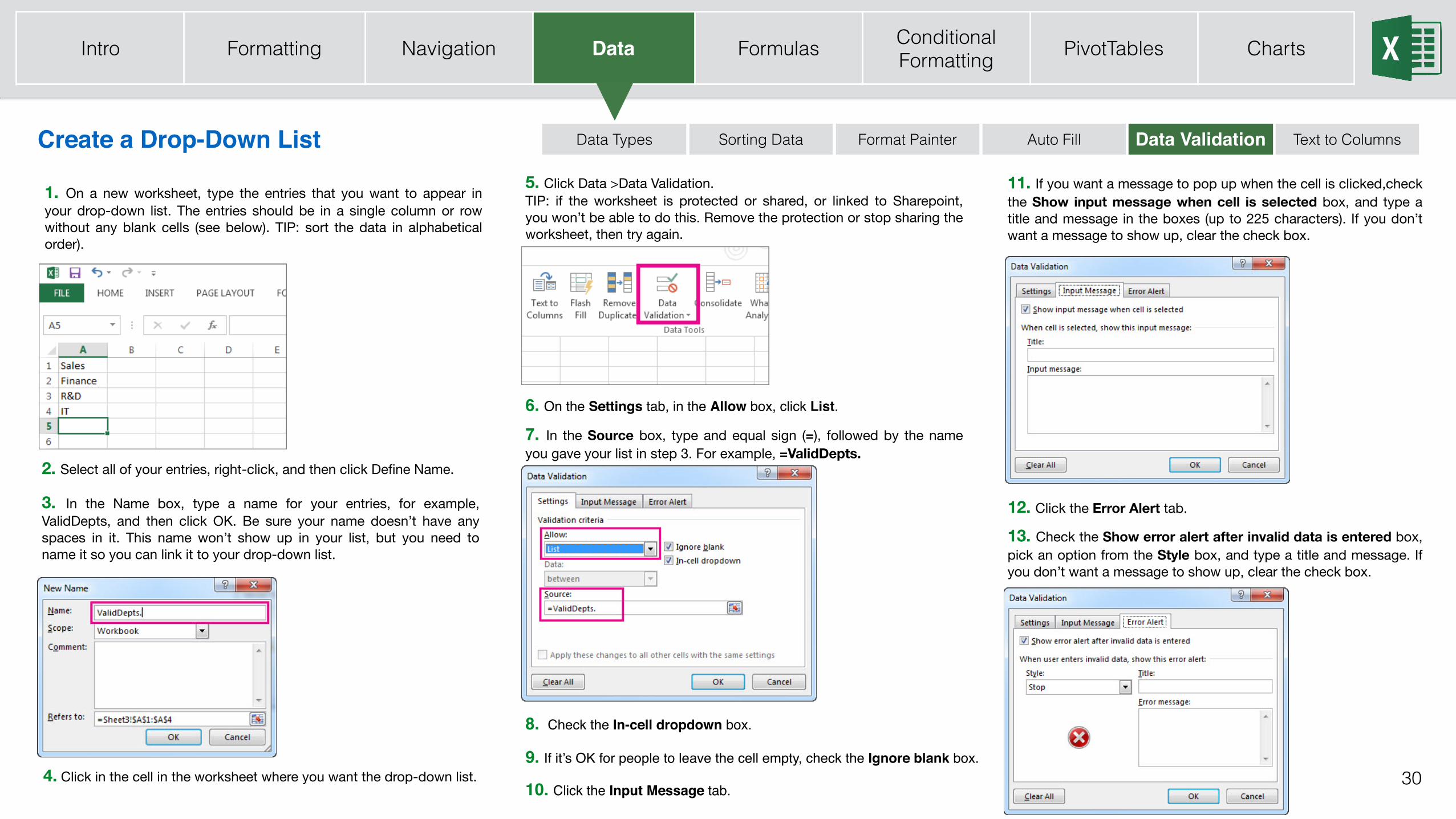
1. On a new worksheet, type the entries that you want to appear in your drop-down list. The entries should be in a single column or row without any blank cells (see below). TIP: sort the data in alphabetical order).
2. Select all of your entries, right-click, and then click Define Name.
3. In the Name box, type a name for your entries, for example, ValidDepts, and then click OK. Be sure your name doesn’t have any spaces in it. This name won’t show up in your list, but you need to name it so you can link it to your drop-down list.
4. Click in the cell in the worksheet where you want the drop-down list.
5. Click Data >Data Validation.TIP: if the worksheet is protected or shared, or linked to Sharepoint, you won’t be able to do this. Remove the protection or stop sharing the worksheet, then try again.
6. On the Settings tab, in the Allow box, click List.
8. Check the In-cell dropdown box.
9. If it’s OK for people to leave the cell empty, check the Ignore blank box.
10. Click the Input Message tab.
12. Click the Error Alert tab.
11. If you want a message to pop up when the cell is clicked,check the Show input message when cell is selected box, and type a title and message in the boxes (up to 225 characters). If you don’t want a message to show up, clear the check box.
13. Check the Show error alert after invalid data is entered box, pick an option from the Style box, and type a title and message. If you don’t want a message to show up, clear the check box.
7. In the Source box, type and equal sign (=), followed by the name you gave your list in step 3. For example, =ValidDepts.
Intro Formatting Navigation Data Formulas Conditional Formatting PivotTables Charts
31
Auto Fill Data ValidationSorting Data Text to ColumnsFormat PainterData TypesText to Columns
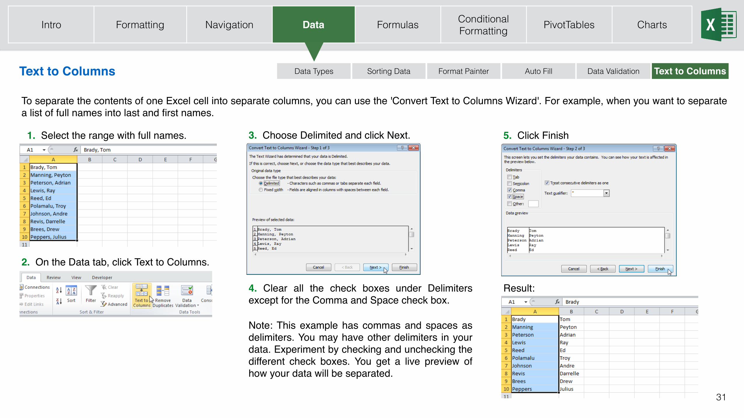
To separate the contents of one Excel cell into separate columns, you can use the 'Convert Text to Columns Wizard'. For example, when you want to separate a list of full names into last and first names.
2. On the Data tab, click Text to Columns.
3. Choose Delimited and click Next. 1. Select the range with full names.
4. Clear all the check boxes under Delimiters except for the Comma and Space check box.
5. Click Finish
Note: This example has commas and spaces as delimiters. You may have other delimiters in your data. Experiment by checking and unchecking the different check boxes. You get a live preview of how your data will be separated.
Result:
Intro Formatting Navigation Data Formulas Conditional Formatting PivotTables Charts
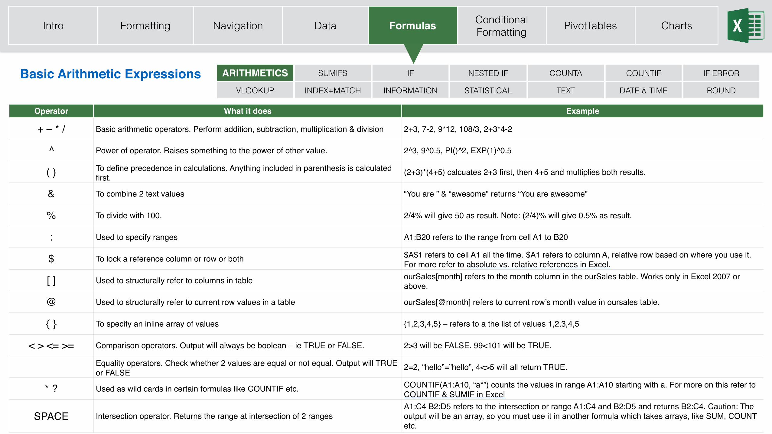
Operator What it does Example
+ – * / Basic arithmetic operators. Perform addition, subtraction, multiplication & division 2+3, 7-2, 9*12, 108/3, 2+3*4-2
^ Power of operator. Raises something to the power of other value. 2^3, 9^0.5, PI()^2, EXP(1)^0.5
( ) To define precedence in calculations. Anything included in parenthesis is calculated first. (2+3)*(4+5) calcuates 2+3 first, then 4+5 and multiplies both results.
& To combine 2 text values “You are ” & “awesome” returns “You are awesome”
% To divide with 100. 2/4% will give 50 as result. Note: (2/4)% will give 0.5% as result.
: Used to specify ranges A1:B20 refers to the range from cell A1 to B20
$ To lock a reference column or row or both $A$1 refers to cell A1 all the time. $A1 refers to column A, relative row based on where you use it. For more refer to absolute vs. relative references in Excel.
[ ] Used to structurally refer to columns in table ourSales[month] refers to the month column in the ourSales table. Works only in Excel 2007 or above.
@ Used to structurally refer to current row values in a table ourSales[@month] refers to current row’s month value in oursales table.
{ } To specify an inline array of values {1,2,3,4,5} – refers to a the list of values 1,2,3,4,5
< > <= >= Comparison operators. Output will always be boolean – ie TRUE or FALSE. 2>3 will be FALSE. 99<101 will be TRUE.
Equality operators. Check whether 2 values are equal or not equal. Output will TRUE or FALSE 2=2, “hello”=”hello”, 4<>5 will all return TRUE.
* ? Used as wild cards in certain formulas like COUNTIF etc. COUNTIF(A1:A10, “a*”) counts the values in range A1:A10 starting with a. For more on this refer to COUNTIF & SUMIF in Excel
SPACE Intersection operator. Returns the range at intersection of 2 rangesA1:C4 B2:D5 refers to the intersection or range A1:C4 and B2:D5 and returns B2:C4. Caution: The output will be an array, so you must use it in another formula which takes arrays, like SUM, COUNT etc.
Basic Arithmetic Expressions
Intro Formatting Navigation Data Formulas Conditional Formatting PivotTables Charts
INDEX+MATCH
COUNTAIF NESTED IFSUMIFSARITHMETICSTEXTSTATISTICAL
IF ERROR
DATE & TIME
COUNTIF
VLOOKUP INFORMATION ROUND
33
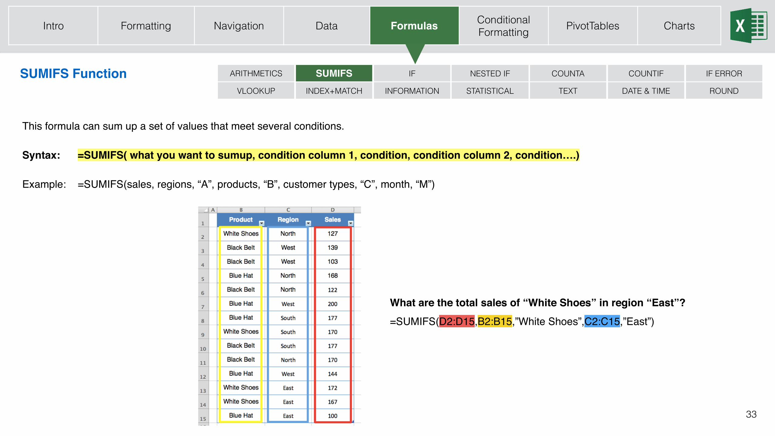
This formula can sum up a set of values that meet several conditions.
Syntax: =SUMIFS( what you want to sumup, condition column 1, condition, condition column 2, condition….)
Example: =SUMIFS(sales, regions, “A”, products, “B”, customer types, “C”, month, “M”)
SUMIFS Function
What are the total sales of “White Shoes” in region “East”?=SUMIFS(D2:D15,B2:B15,”White Shoes”,C2:C15,”East”)
INDEX+MATCH
COUNTAIF NESTED IFSUMIFSARITHMETICS
TEXTSTATISTICAL
IF ERROR
DATE & TIME
COUNTIF
VLOOKUP INFORMATION ROUND
Intro Formatting Navigation Data Formulas Conditional Formatting PivotTables Charts
34
IF Function
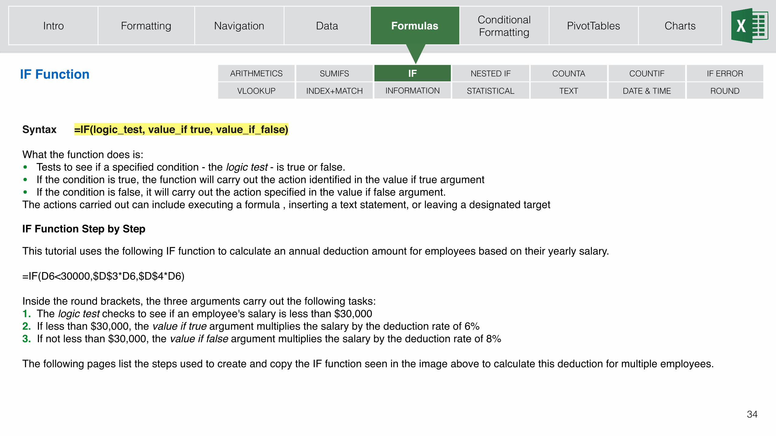
Syntax =IF(logic_test, value_if true, value_if_false)
What the function does is:• Tests to see if a specified condition - the logic test - is true or false.• If the condition is true, the function will carry out the action identified in the value if true argument• If the condition is false, it will carry out the action specified in the value if false argument.The actions carried out can include executing a formula , inserting a text statement, or leaving a designated target
IF Function Step by Step
This tutorial uses the following IF function to calculate an annual deduction amount for employees based on their yearly salary.
=IF(D6<30000,$D$3*D6,$D$4*D6)
Inside the round brackets, the three arguments carry out the following tasks:1. The logic test checks to see if an employee's salary is less than $30,0002. If less than $30,000, the value if true argument multiplies the salary by the deduction rate of 6%3. If not less than $30,000, the value if false argument multiplies the salary by the deduction rate of 8%
The following pages list the steps used to create and copy the IF function seen in the image above to calculate this deduction for multiple employees.
INDEX+MATCH
COUNTAIF NESTED IFSUMIFSARITHMETICS
TEXTSTATISTICAL
IF ERROR
DATE & TIME
COUNTIF
VLOOKUP INFORMATION ROUND
Intro Formatting Navigation Data Formulas Conditional Formatting PivotTables Charts
35
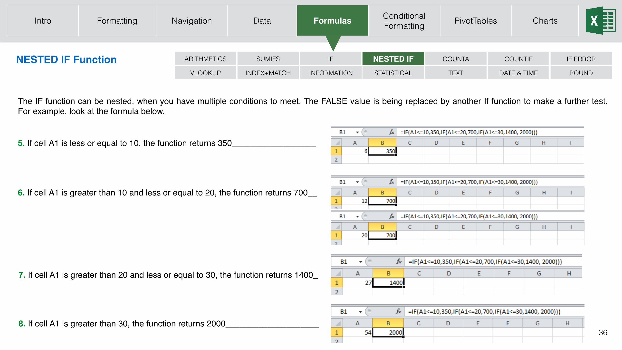
NESTED IF Function
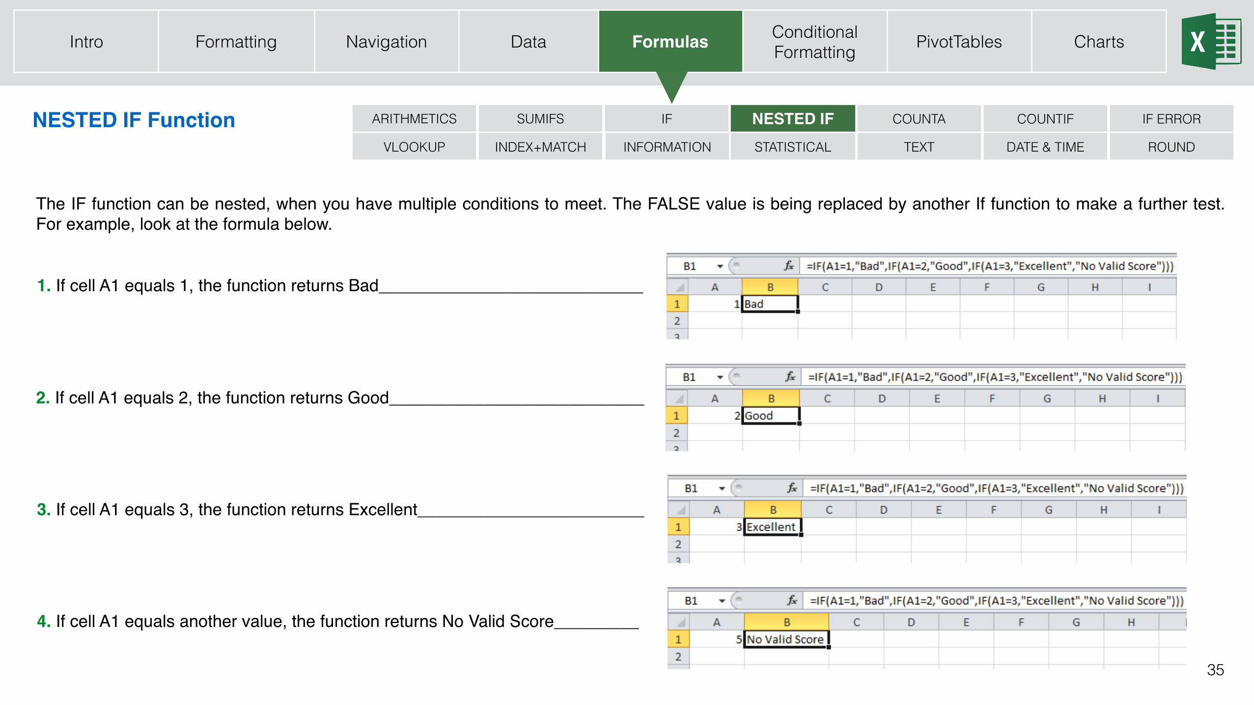
The IF function can be nested, when you have multiple conditions to meet. The FALSE value is being replaced by another If function to make a further test. For example, look at the formula below.
2. If cell A1 equals 2, the function returns Good___________________________
3. If cell A1 equals 3, the function returns Excellent________________________
4. If cell A1 equals another value, the function returns No Valid Score_________
1. If cell A1 equals 1, the function returns Bad____________________________
INDEX+MATCH
COUNTAIF NESTED IFSUMIFSARITHMETICS
TEXTSTATISTICAL
IF ERROR
DATE & TIME
COUNTIF
VLOOKUP INFORMATION ROUND
Intro Formatting Navigation Data Formulas Conditional Formatting PivotTables Charts
36
The IF function can be nested, when you have multiple conditions to meet. The FALSE value is being replaced by another If function to make a further test. For example, look at the formula below.
6. If cell A1 is greater than 10 and less or equal to 20, the function returns 700__
7. If cell A1 is greater than 20 and less or equal to 30, the function returns 1400_
8. If cell A1 is greater than 30, the function returns 2000____________________
5. If cell A1 is less or equal to 10, the function returns 350__________________
INDEX+MATCH
COUNTAIF NESTED IFSUMIFSARITHMETICS
TEXTSTATISTICAL
IF ERROR
DATE & TIME
COUNTIF
VLOOKUP INFORMATION ROUND
NESTED IF Function
Intro Formatting Navigation Data Formulas Conditional Formatting PivotTables Charts
37
COUNTA & COUNTBLANK Functions
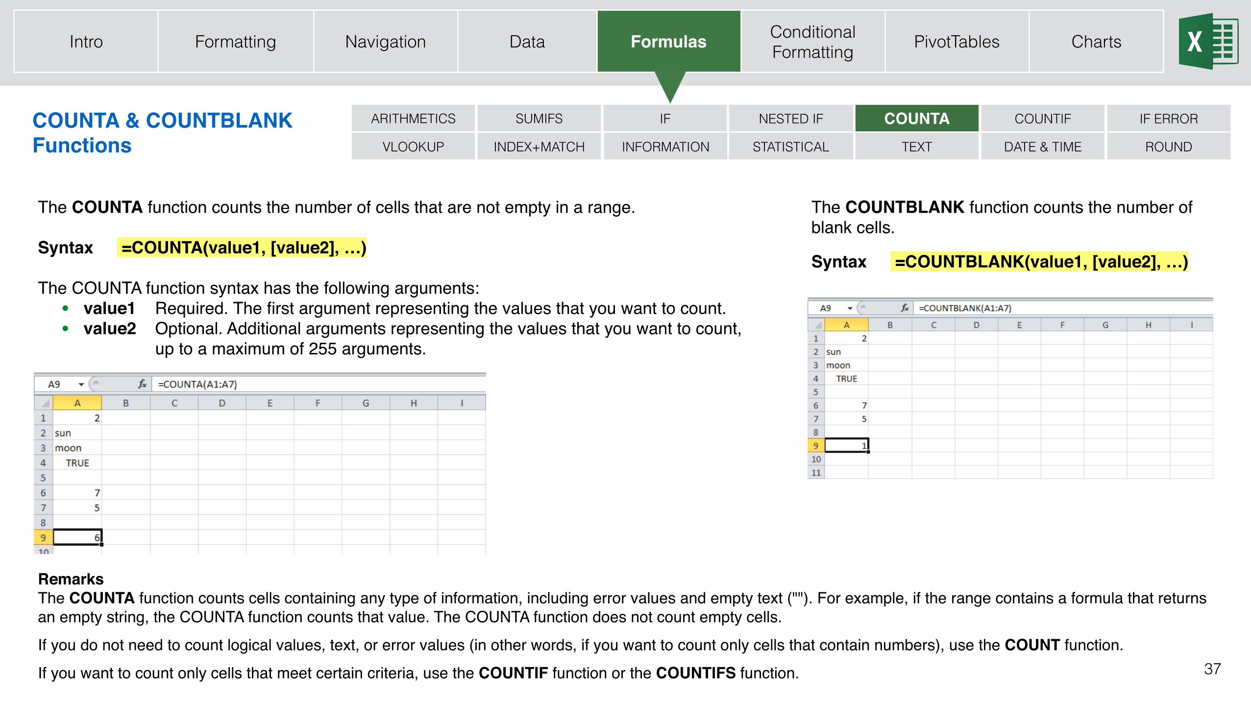
The COUNTA function counts the number of cells that are not empty in a range.
Syntax =COUNTA(value1, [value2], …)
The COUNTA function syntax has the following arguments:• value1 Required. The first argument representing the values that you want to count.• value2 Optional. Additional arguments representing the values that you want to count,
up to a maximum of 255 arguments.
INDEX+MATCH
COUNTAIF NESTED IFSUMIFSARITHMETICS
TEXTSTATISTICAL
IF ERROR
DATE & TIME
COUNTIF
VLOOKUP INFORMATION ROUND
The COUNTBLANK function counts the number of blank cells.
RemarksThe COUNTA function counts cells containing any type of information, including error values and empty text (""). For example, if the range contains a formula that returns an empty string, the COUNTA function counts that value. The COUNTA function does not count empty cells.If you do not need to count logical values, text, or error values (in other words, if you want to count only cells that contain numbers), use the COUNT function.If you want to count only cells that meet certain criteria, use the COUNTIF function or the COUNTIFS function.
Syntax =COUNTBLANK(value1, [value2], …)
Intro Formatting Navigation Data Formulas Conditional Formatting PivotTables Charts
38
COUNTIF & COUNTIFS Functions
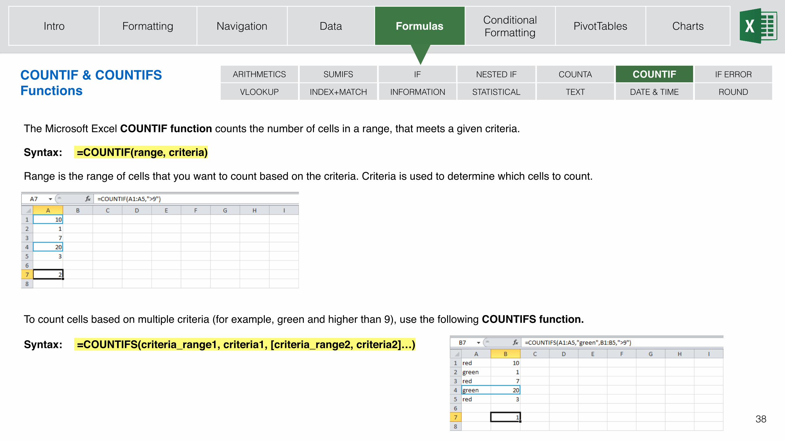
The Microsoft Excel COUNTIF function counts the number of cells in a range, that meets a given criteria.
Syntax: =COUNTIF(range, criteria)
Range is the range of cells that you want to count based on the criteria. Criteria is used to determine which cells to count.
INDEX+MATCH
COUNTAIF NESTED IFSUMIFSARITHMETICS
TEXTSTATISTICAL
IF ERROR
DATE & TIME
COUNTIFVLOOKUP INFORMATION ROUND
To count cells based on multiple criteria (for example, green and higher than 9), use the following COUNTIFS function.
Syntax: =COUNTIFS(criteria_range1, criteria1, [criteria_range2, criteria2]…)
Intro Formatting Navigation Data Formulas Conditional Formatting PivotTables Charts
39
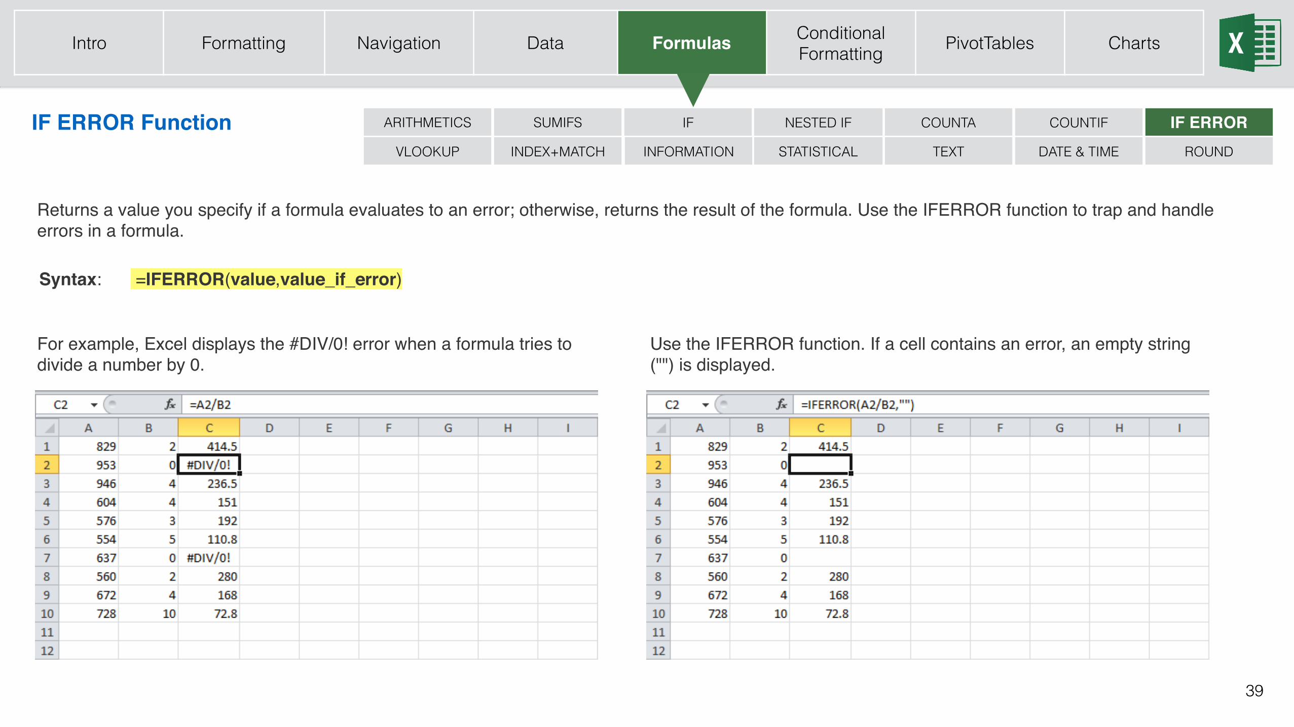
IF ERROR Function
Returns a value you specify if a formula evaluates to an error; otherwise, returns the result of the formula. Use the IFERROR function to trap and handle errors in a formula.
Syntax: =IFERROR(value,value_if_error)
For example, Excel displays the #DIV/0! error when a formula tries to divide a number by 0.
Use the IFERROR function. If a cell contains an error, an empty string ("") is displayed.
INDEX+MATCH
COUNTAIF NESTED IFSUMIFSARITHMETICS
TEXTSTATISTICAL
IF ERRORDATE & TIME
COUNTIF
VLOOKUP INFORMATION ROUND
Intro Formatting Navigation Data Formulas Conditional Formatting PivotTables Charts
40
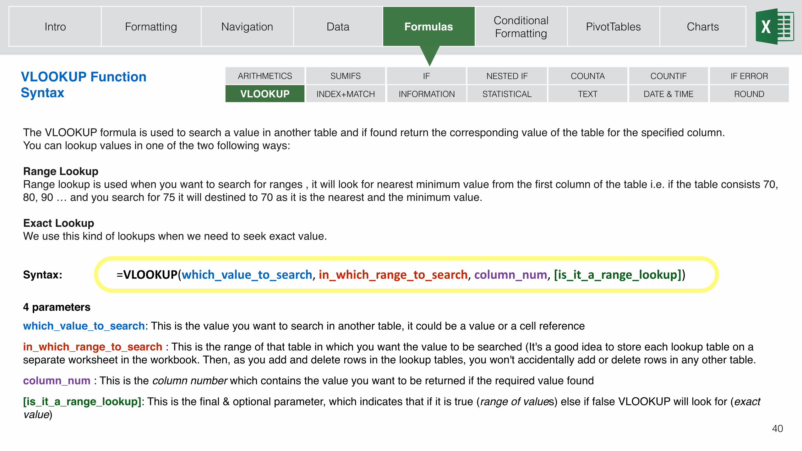
VLOOKUP FunctionSyntax
The VLOOKUP formula is used to search a value in another table and if found return the corresponding value of the table for the specified column. You can lookup values in one of the two following ways:
Range LookupRange lookup is used when you want to search for ranges , it will look for nearest minimum value from the first column of the table i.e. if the table consists 70, 80, 90 … and you search for 75 it will destined to 70 as it is the nearest and the minimum value.
Exact LookupWe use this kind of lookups when we need to seek exact value.
=VLOOKUP(which_value_to_search, in_which_range_to_search, column_num, [is_it_a_range_lookup])
4 parameterswhich_value_to_search: This is the value you want to search in another table, it could be a value or a cell reference
in_which_range_to_search : This is the range of that table in which you want the value to be searched (It's a good idea to store each lookup table on a separate worksheet in the workbook. Then, as you add and delete rows in the lookup tables, you won't accidentally add or delete rows in any other table.
column_num : This is the column number which contains the value you want to be returned if the required value found
[is_it_a_range_lookup]: This is the final & optional parameter, which indicates that if it is true (range of values) else if false VLOOKUP will look for (exact value)
Syntax:
INDEX+MATCH
COUNTAIF NESTED IFSUMIFSARITHMETICS
TEXTSTATISTICAL
IF ERROR
DATE & TIME
COUNTIF
VLOOKUP INFORMATION ROUND
Intro Formatting Navigation Data Formulas Conditional Formatting PivotTables Charts

41
A lookup table includes the values you wish to “lookup”. You can place this table on the same worksheet, however it is recommended to create a new worksheet.
How to Create the Lookup Table:1. Right-click your spreadsheet’s tab and select Insert…2. On the Insert dialog, double-click Worksheet. This will be on the General tab.3. Rename this new worksheet tab (a descriptive name or a generic name such as VLOOKUP)4. In Column A, enter the unique values that exist on your main worksheet.5. In Column B, enter the translated value. You can have more values in column A than appear on your main spreadsheet.
VLOOKUP FunctionCreate a Table
Using the Function
1. Add your new column on your original worksheet that will display the info pulled from the Lookup table.2. Place your cursor in the first blank cell in that column.3. From the Insert menu, select Function…. Select the VLOOKP function and fill in the arguments.4. Using Auto Fill, copy the formula down in the rest of column. Note: before doing so, remember to change the cell references from relative to absolute.
Place the cursor immediately before the value and press F4. For example, if the range in the VLOOKP table is A1:B9, the corresponding absolute values will be $A$1:$B$9.
INDEX+MATCH
COUNTAIF NESTED IFSUMIFSARITHMETICS
TEXTSTATISTICAL
IF ERROR
DATE & TIME
COUNTIF
VLOOKUP INFORMATION ROUND
Intro Formatting Navigation Data Formulas Conditional Formatting PivotTables Charts
42
INDEX+MATCH Function
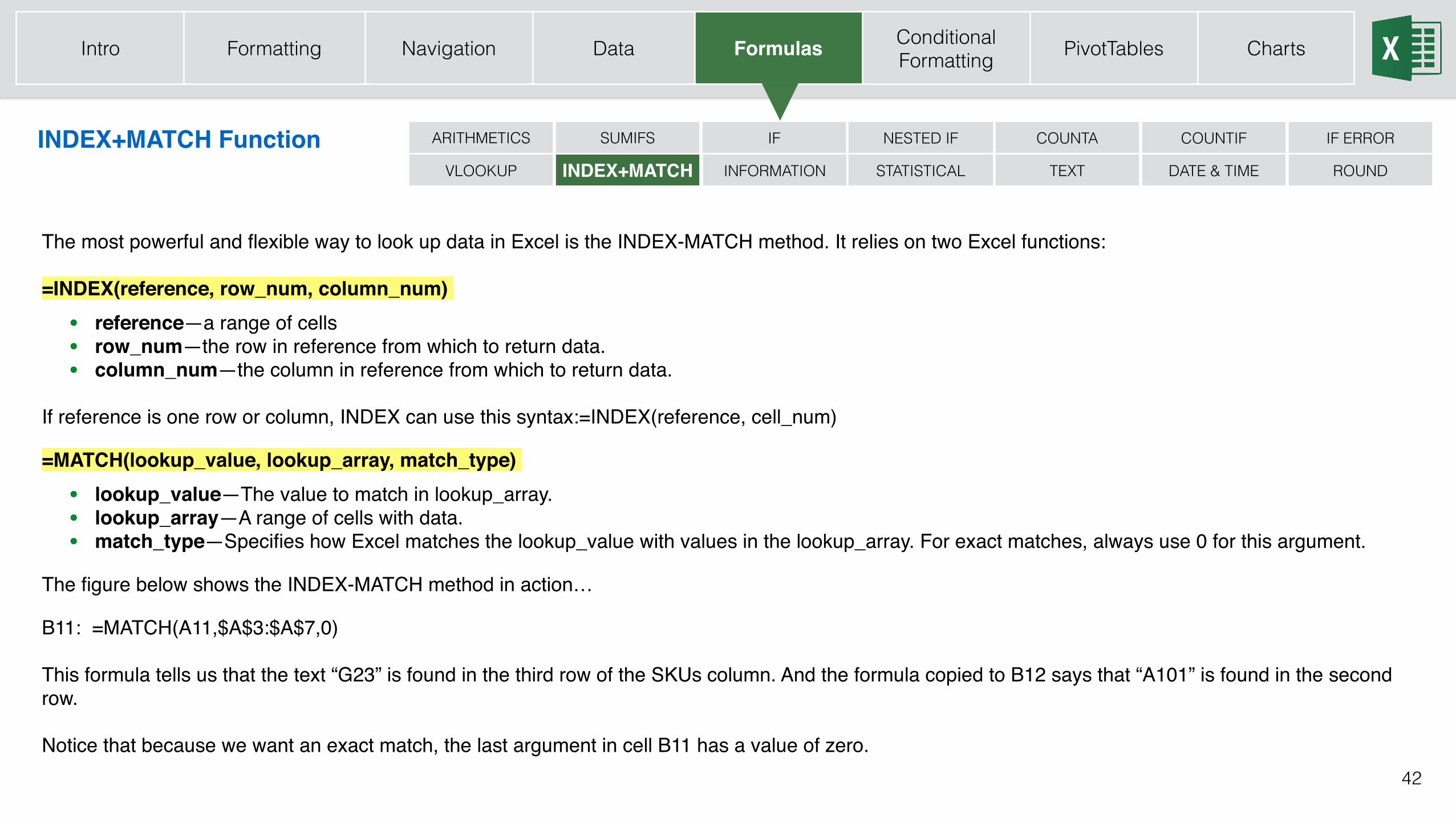
The most powerful and flexible way to look up data in Excel is the INDEX-MATCH method. It relies on two Excel functions:
=INDEX(reference, row_num, column_num)
• reference—a range of cells• row_num—the row in reference from which to return data.• column_num—the column in reference from which to return data.
If reference is one row or column, INDEX can use this syntax:=INDEX(reference, cell_num)
=MATCH(lookup_value, lookup_array, match_type)
• lookup_value—The value to match in lookup_array.• lookup_array—A range of cells with data.• match_type—Specifies how Excel matches the lookup_value with values in the lookup_array. For exact matches, always use 0 for this argument.
The figure below shows the INDEX-MATCH method in action…
B11: =MATCH(A11,$A$3:$A$7,0)
This formula tells us that the text “G23” is found in the third row of the SKUs column. And the formula copied to B12 says that “A101” is found in the second row.
Notice that because we want an exact match, the last argument in cell B11 has a value of zero.
INDEX+MATCH
COUNTAIF NESTED IFSUMIFSARITHMETICS
TEXTSTATISTICAL
IF ERROR
DATE & TIME
COUNTIF
VLOOKUP INFORMATION ROUND
Intro Formatting Navigation Data Formulas Conditional Formatting PivotTables Charts
43
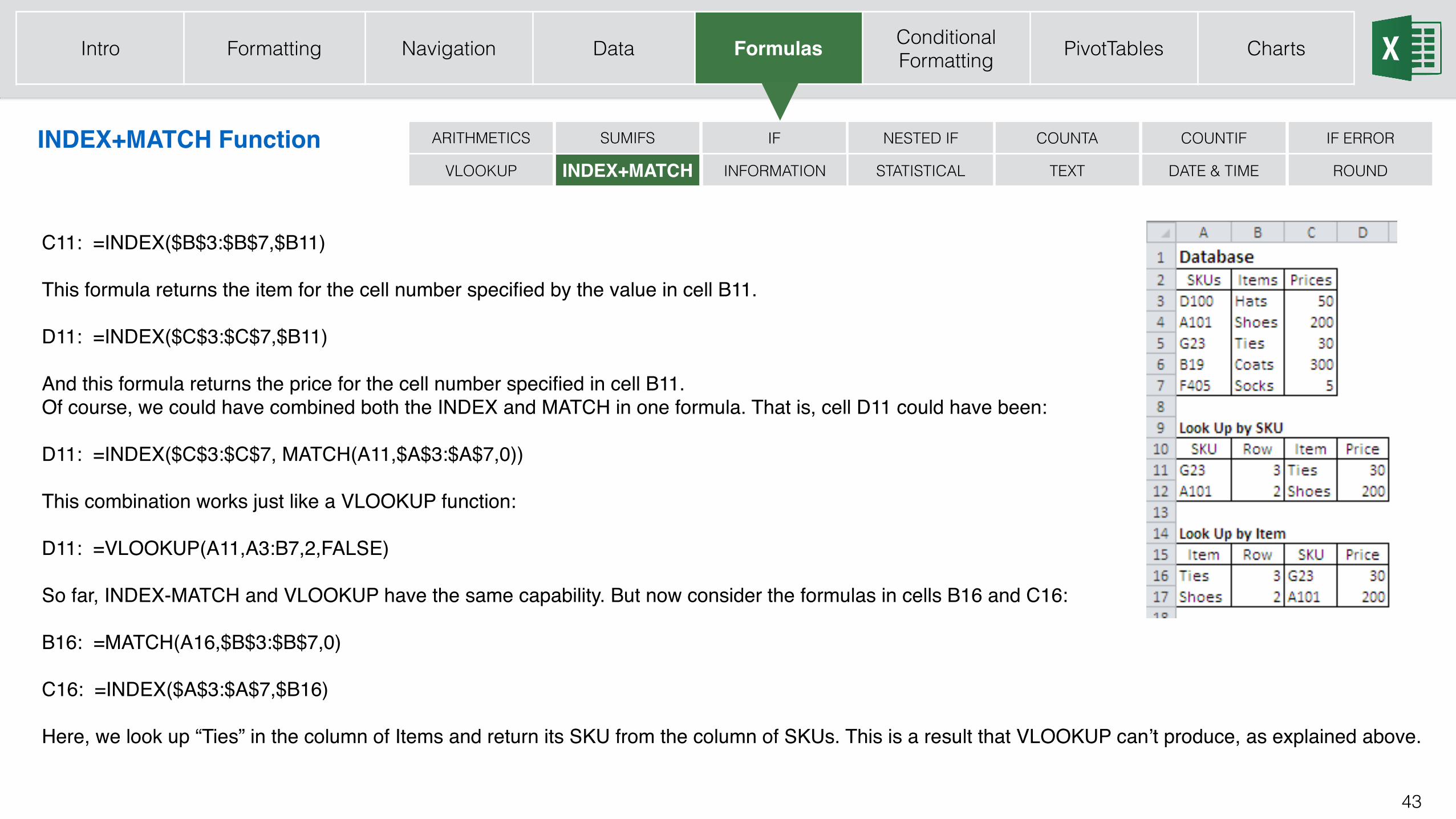
INDEX+MATCH Function
C11: =INDEX($B$3:$B$7,$B11)
This formula returns the item for the cell number specified by the value in cell B11.
D11: =INDEX($C$3:$C$7,$B11)
And this formula returns the price for the cell number specified in cell B11.Of course, we could have combined both the INDEX and MATCH in one formula. That is, cell D11 could have been:
D11: =INDEX($C$3:$C$7, MATCH(A11,$A$3:$A$7,0))
This combination works just like a VLOOKUP function:
D11: =VLOOKUP(A11,A3:B7,2,FALSE)
So far, INDEX-MATCH and VLOOKUP have the same capability. But now consider the formulas in cells B16 and C16:
B16: =MATCH(A16,$B$3:$B$7,0)
C16: =INDEX($A$3:$A$7,$B16)
Here, we look up “Ties” in the column of Items and return its SKU from the column of SKUs. This is a result that VLOOKUP can’t produce, as explained above.
INDEX+MATCH
COUNTAIF NESTED IFSUMIFSARITHMETICS
TEXTSTATISTICAL
IF ERROR
DATE & TIME
COUNTIF
VLOOKUP INFORMATION ROUND
Intro Formatting Navigation Data Formulas Conditional Formatting PivotTables Charts
44
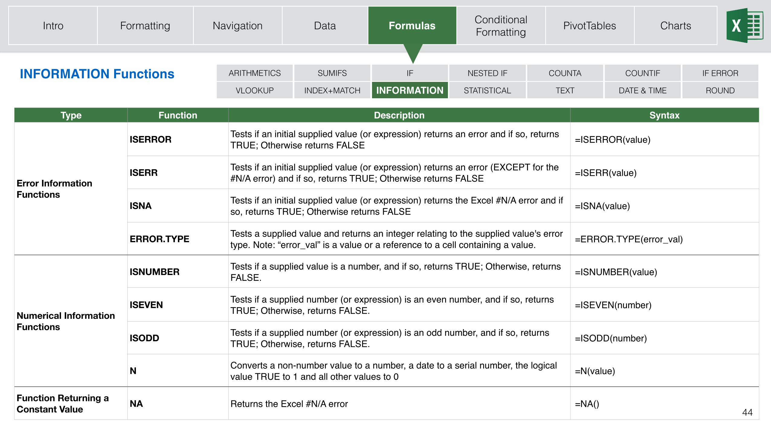
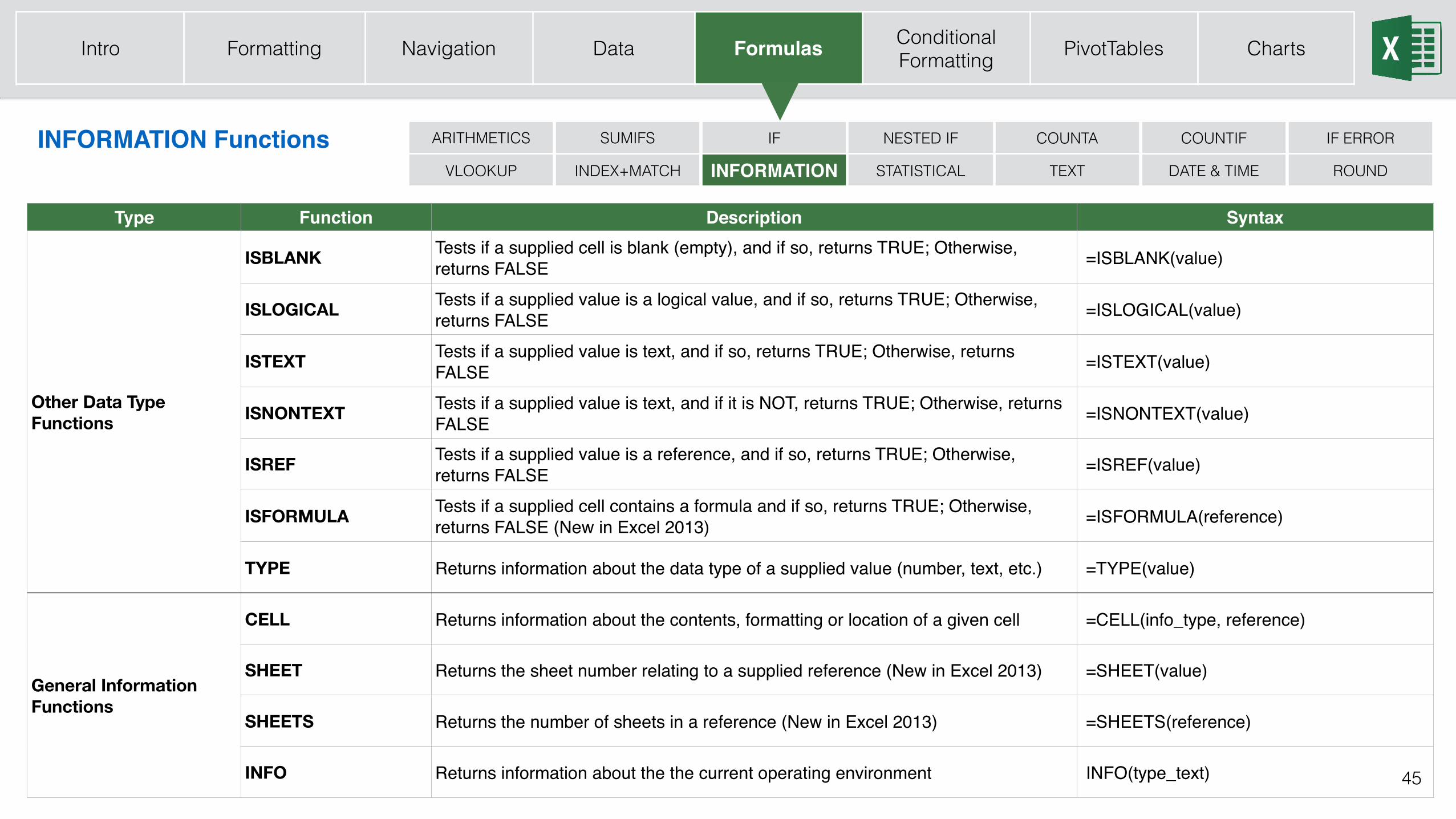
INFORMATION Functions
Type Function Description Syntax
Error Information Functions
ISERROR Tests if an initial supplied value (or expression) returns an error and if so, returns TRUE; Otherwise returns FALSE =ISERROR(value)
ISERR Tests if an initial supplied value (or expression) returns an error (EXCEPT for the #N/A error) and if so, returns TRUE; Otherwise returns FALSE =ISERR(value)
ISNA Tests if an initial supplied value (or expression) returns the Excel #N/A error and if so, returns TRUE; Otherwise returns FALSE =ISNA(value)
ERROR.TYPE Tests a supplied value and returns an integer relating to the supplied value's error type. Note: “error_val” is a value or a reference to a cell containing a value. =ERROR.TYPE(error_val)
Numerical Information Functions
ISNUMBER Tests if a supplied value is a number, and if so, returns TRUE; Otherwise, returns FALSE. =ISNUMBER(value)
ISEVEN Tests if a supplied number (or expression) is an even number, and if so, returns TRUE; Otherwise, returns FALSE. =ISEVEN(number)
ISODD Tests if a supplied number (or expression) is an odd number, and if so, returns TRUE; Otherwise, returns FALSE. =ISODD(number)
N Converts a non-number value to a number, a date to a serial number, the logical value TRUE to 1 and all other values to 0 =N(value)
Function Returning a Constant Value NA Returns the Excel #N/A error =NA()
INDEX+MATCH
COUNTAIF NESTED IFSUMIFSARITHMETICS
TEXTSTATISTICAL
IF ERROR
DATE & TIME
COUNTIF
VLOOKUP INFORMATION ROUND
Intro Formatting Navigation Data Formulas Conditional Formatting PivotTables Charts
45
INDEX+MATCH
COUNTAIF NESTED IFSUMIFSARITHMETICS
TEXTSTATISTICAL
IF ERROR
DATE & TIME
COUNTIF
VLOOKUP INFORMATIONINFORMATION Functions
Type Function Description Syntax
Other Data Type Functions
ISBLANK Tests if a supplied cell is blank (empty), and if so, returns TRUE; Otherwise, returns FALSE =ISBLANK(value)
ISLOGICAL Tests if a supplied value is a logical value, and if so, returns TRUE; Otherwise, returns FALSE =ISLOGICAL(value)
ISTEXT Tests if a supplied value is text, and if so, returns TRUE; Otherwise, returns FALSE =ISTEXT(value)
ISNONTEXT Tests if a supplied value is text, and if it is NOT, returns TRUE; Otherwise, returns FALSE =ISNONTEXT(value)
ISREF Tests if a supplied value is a reference, and if so, returns TRUE; Otherwise, returns FALSE =ISREF(value)
ISFORMULA Tests if a supplied cell contains a formula and if so, returns TRUE; Otherwise, returns FALSE (New in Excel 2013) =ISFORMULA(reference)
TYPE Returns information about the data type of a supplied value (number, text, etc.) =TYPE(value)
General Information Functions
CELL Returns information about the contents, formatting or location of a given cell =CELL(info_type, reference)
SHEET Returns the sheet number relating to a supplied reference (New in Excel 2013) =SHEET(value)
SHEETS Returns the number of sheets in a reference (New in Excel 2013) =SHEETS(reference)
INFO Returns information about the the current operating environment INFO(type_text)
ROUND
Intro Formatting Navigation Data Formulas Conditional Formatting PivotTables Charts
46
INDEX+MATCH
COUNTAIF NESTED IFSUMIFSARITHMETICS
TEXTSTATISTICAL
IF ERROR
DATE & TIME
COUNTIF
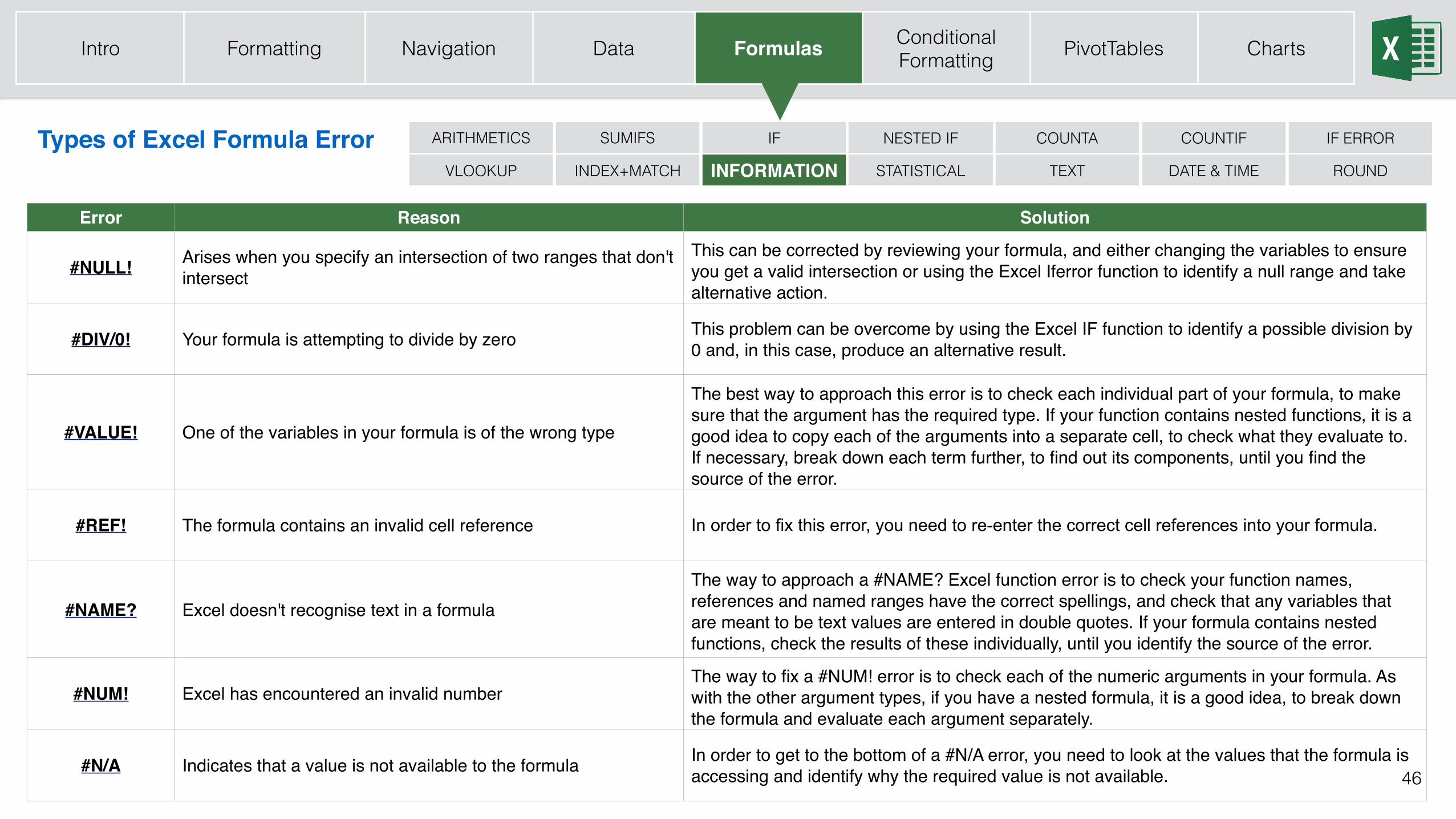
VLOOKUP INFORMATIONTypes of Excel Formula Error
ROUND
Error Reason Solution
#NULL! Arises when you specify an intersection of two ranges that don't intersect
This can be corrected by reviewing your formula, and either changing the variables to ensure you get a valid intersection or using the Excel Iferror function to identify a null range and take alternative action.
#DIV/0! Your formula is attempting to divide by zero This problem can be overcome by using the Excel IF function to identify a possible division by 0 and, in this case, produce an alternative result.
#VALUE! One of the variables in your formula is of the wrong type
The best way to approach this error is to check each individual part of your formula, to make sure that the argument has the required type. If your function contains nested functions, it is a good idea to copy each of the arguments into a separate cell, to check what they evaluate to. If necessary, break down each term further, to find out its components, until you find the source of the error.
#REF! The formula contains an invalid cell reference In order to fix this error, you need to re-enter the correct cell references into your formula.
#NAME? Excel doesn't recognise text in a formulaThe way to approach a #NAME? Excel function error is to check your function names, references and named ranges have the correct spellings, and check that any variables that are meant to be text values are entered in double quotes. If your formula contains nested functions, check the results of these individually, until you identify the source of the error.
#NUM! Excel has encountered an invalid numberThe way to fix a #NUM! error is to check each of the numeric arguments in your formula. As with the other argument types, if you have a nested formula, it is a good idea, to break down the formula and evaluate each argument separately.
#N/A Indicates that a value is not available to the formula In order to get to the bottom of a #N/A error, you need to look at the values that the formula is accessing and identify why the required value is not available.
Intro Formatting Navigation Data Formulas Conditional Formatting PivotTables Charts
47
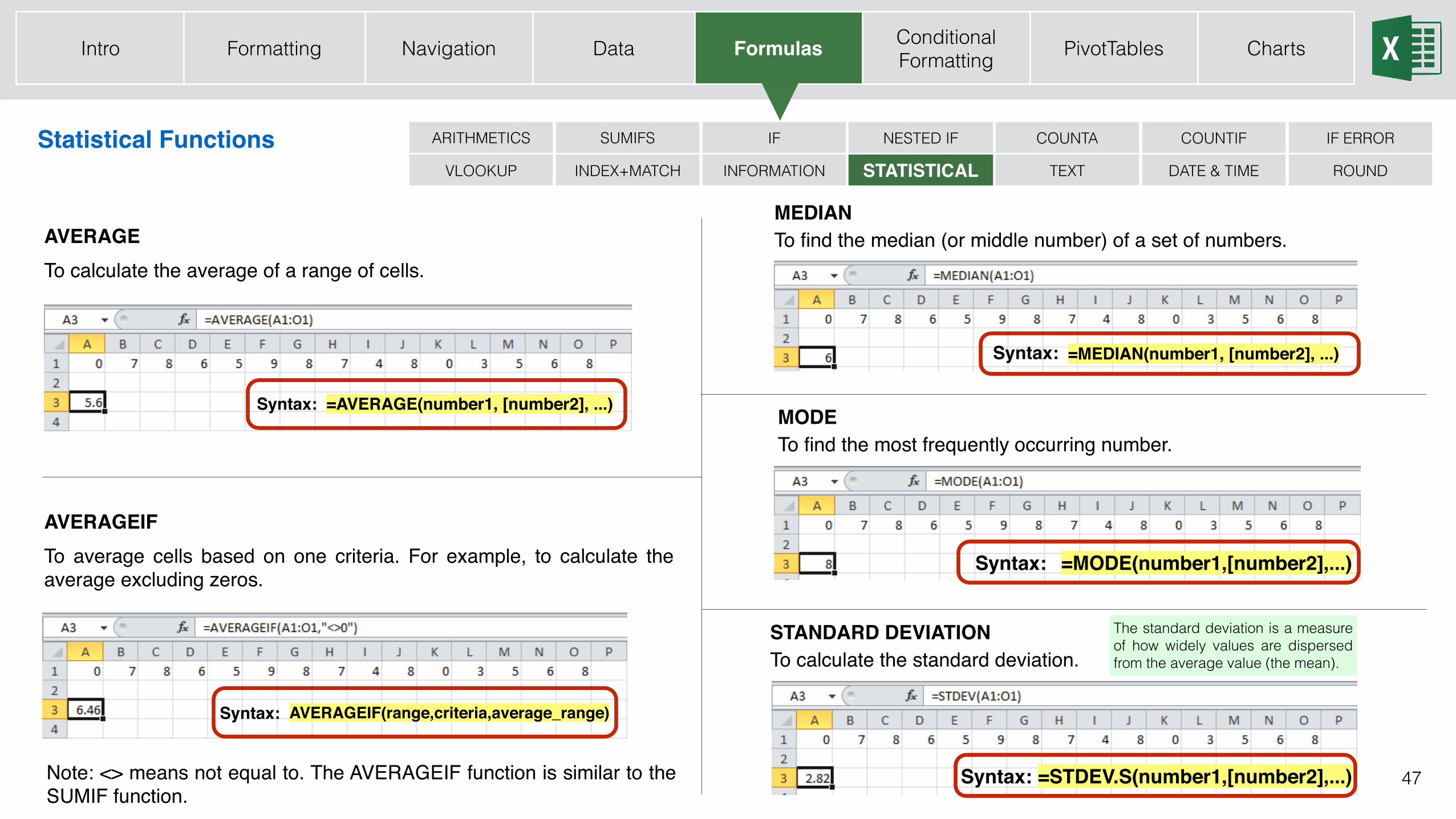
Statistical Functions
AVERAGETo calculate the average of a range of cells.
AVERAGEIFTo average cells based on one criteria. For example, to calculate the average excluding zeros.
Note: <> means not equal to. The AVERAGEIF function is similar to the SUMIF function.
MEDIANTo find the median (or middle number) of a set of numbers.
MODETo find the most frequently occurring number.
STANDARD DEVIATIONTo calculate the standard deviation.
Syntax: =MEDIAN(number1, [number2], ...)
Syntax: =MODE(number1,[number2],...)
Syntax: =AVERAGE(number1, [number2], ...)
AVERAGEIF(range,criteria,average_range)Syntax:
Syntax: =STDEV.S(number1,[number2],...)
The standard deviation is a measure of how widely values are dispersed from the average value (the mean).
INDEX+MATCH
COUNTAIF NESTED IFSUMIFSARITHMETICS
TEXTSTATISTICAL
IF ERROR
DATE & TIME
COUNTIF
VLOOKUP INFORMATION ROUND
Intro Formatting Navigation Data Formulas Conditional Formatting PivotTables Charts
48
Statistical Functions
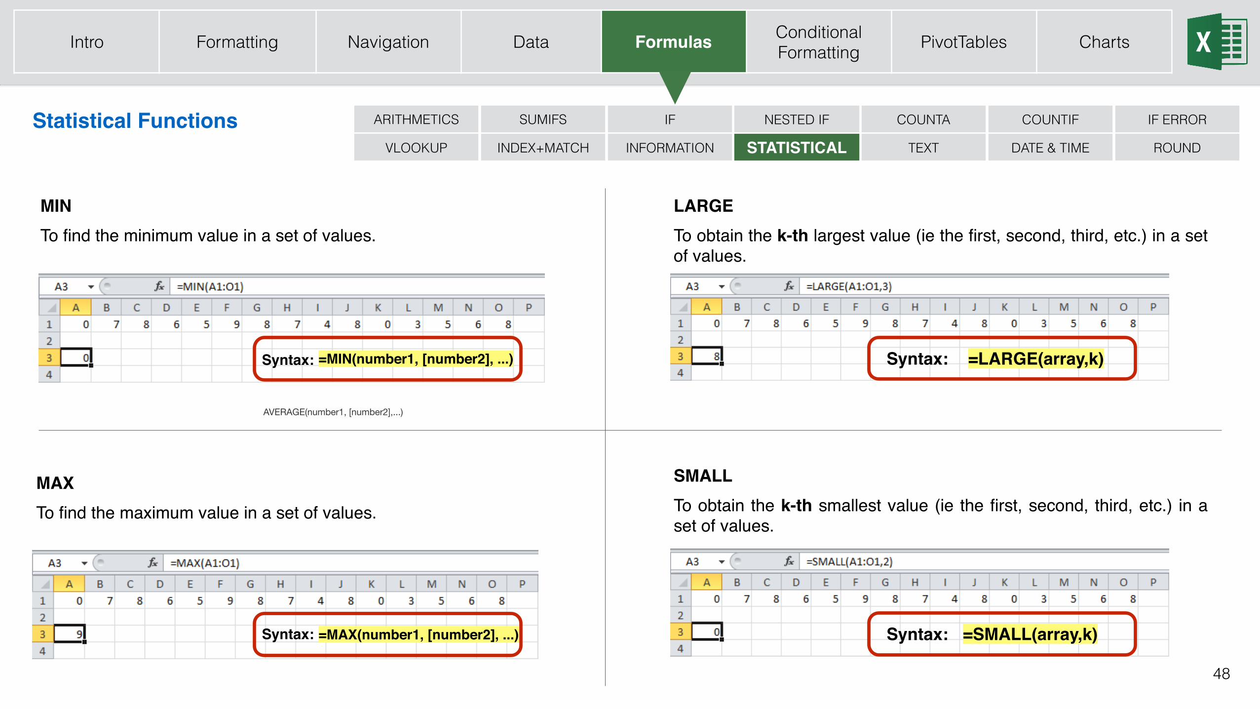
MINTo find the minimum value in a set of values.
MAXTo find the maximum value in a set of values.
LARGETo obtain the k-th largest value (ie the first, second, third, etc.) in a set of values.
Syntax: =MIN(number1, [number2], ...) Syntax: =LARGE(array,k)
Syntax: =SMALL(array,k)Syntax: =MAX(number1, [number2], ...)
SMALLTo obtain the k-th smallest value (ie the first, second, third, etc.) in a set of values.
AVERAGE(number1, [number2],...)
INDEX+MATCH
COUNTAIF NESTED IFSUMIFSARITHMETICS
TEXTSTATISTICAL
IF ERROR
DATE & TIME
COUNTIF
VLOOKUP INFORMATION ROUND
Intro Formatting Navigation Data Formulas Conditional Formatting PivotTables Charts
49
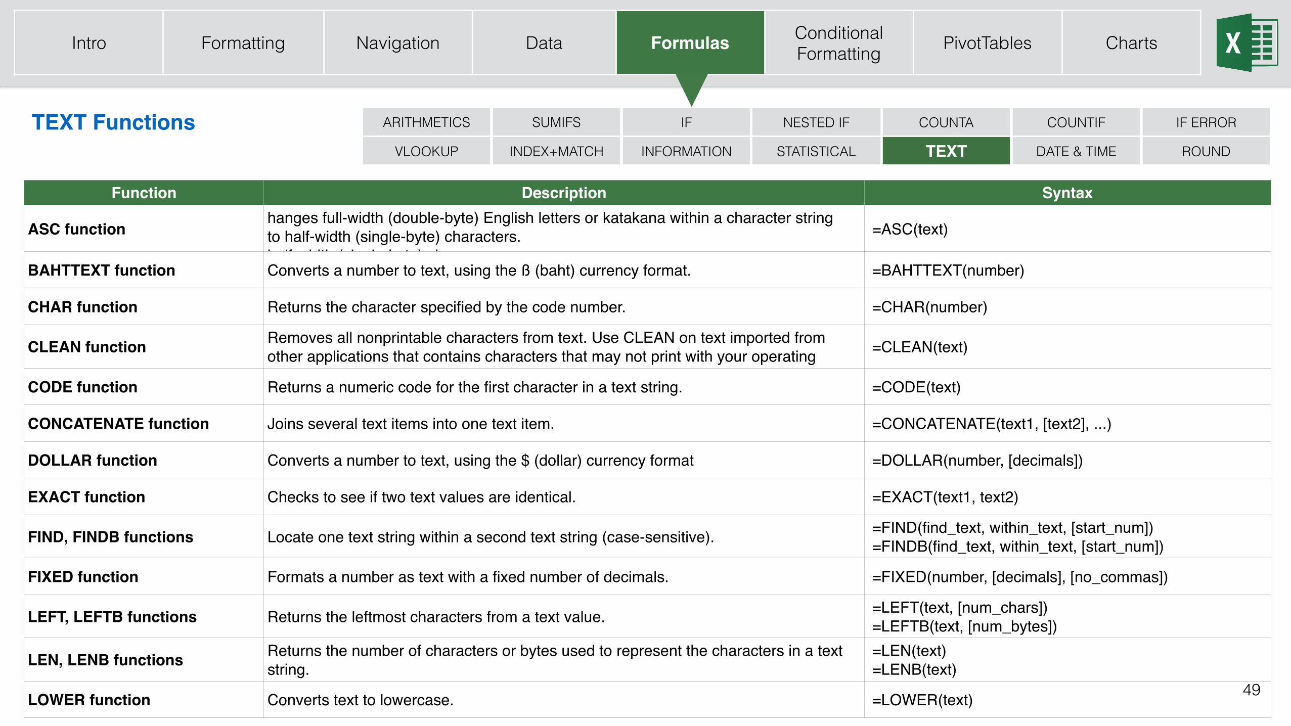
TEXT Functions
Function Description Syntax
ASC functionhanges full-width (double-byte) English letters or katakana within a character string to half-width (single-byte) characters.half-width (single-byte) charac.
=ASC(text)
BAHTTEXT function Converts a number to text, using the ß (baht) currency format. =BAHTTEXT(number)
CHAR function Returns the character specified by the code number. =CHAR(number)
CLEAN function Removes all nonprintable characters from text. Use CLEAN on text imported from other applications that contains characters that may not print with your operating system.
=CLEAN(text)
CODE function Returns a numeric code for the first character in a text string. =CODE(text)
CONCATENATE function Joins several text items into one text item. =CONCATENATE(text1, [text2], ...)
DOLLAR function Converts a number to text, using the $ (dollar) currency format =DOLLAR(number, [decimals])
EXACT function Checks to see if two text values are identical. =EXACT(text1, text2)
FIND, FINDB functions Locate one text string within a second text string (case-sensitive). =FIND(find_text, within_text, [start_num]) =FINDB(find_text, within_text, [start_num])
FIXED function Formats a number as text with a fixed number of decimals. =FIXED(number, [decimals], [no_commas])
LEFT, LEFTB functions Returns the leftmost characters from a text value. =LEFT(text, [num_chars]) =LEFTB(text, [num_bytes])
LEN, LENB functions Returns the number of characters or bytes used to represent the characters in a text string.
=LEN(text) =LENB(text)
LOWER function Converts text to lowercase. =LOWER(text)
INDEX+MATCH
COUNTAIF NESTED IFSUMIFSARITHMETICS
TEXTSTATISTICAL
IF ERROR
DATE & TIME
COUNTIF
VLOOKUP INFORMATION ROUND
Intro Formatting Navigation Data Formulas Conditional Formatting PivotTables Charts
50
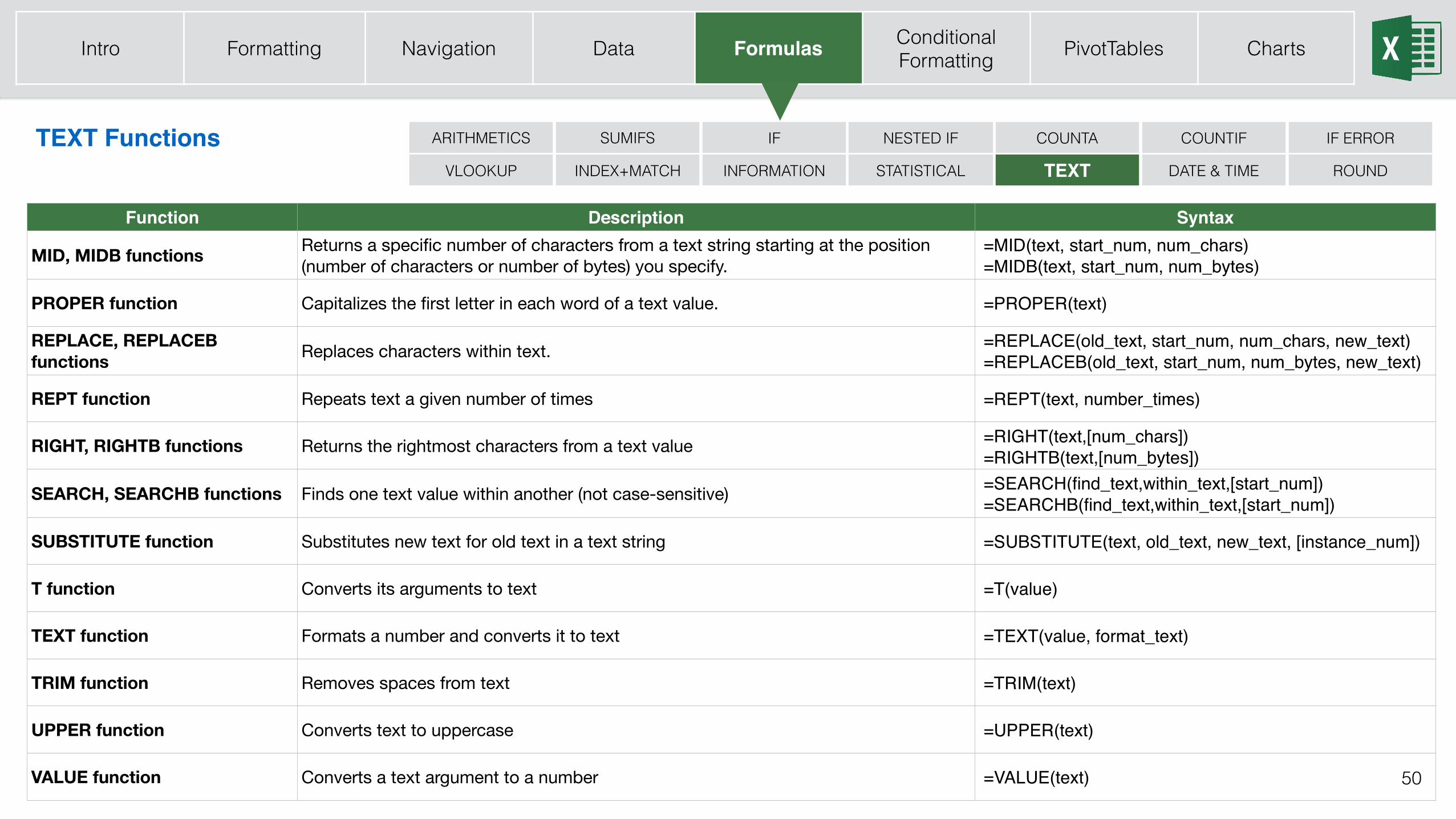
TEXT Functions
Function Description Syntax
MID, MIDB functions Returns a specific number of characters from a text string starting at the position (number of characters or number of bytes) you specify.
=MID(text, start_num, num_chars) =MIDB(text, start_num, num_bytes)
PROPER function Capitalizes the first letter in each word of a text value. =PROPER(text)
REPLACE, REPLACEB functions Replaces characters within text. =REPLACE(old_text, start_num, num_chars, new_text)
=REPLACEB(old_text, start_num, num_bytes, new_text)
REPT function Repeats text a given number of times =REPT(text, number_times)
RIGHT, RIGHTB functions Returns the rightmost characters from a text value =RIGHT(text,[num_chars]) =RIGHTB(text,[num_bytes])
SEARCH, SEARCHB functions Finds one text value within another (not case-sensitive) =SEARCH(find_text,within_text,[start_num]) =SEARCHB(find_text,within_text,[start_num])
SUBSTITUTE function Substitutes new text for old text in a text string =SUBSTITUTE(text, old_text, new_text, [instance_num])
T function Converts its arguments to text =T(value)
TEXT function Formats a number and converts it to text =TEXT(value, format_text)
TRIM function Removes spaces from text =TRIM(text)
UPPER function Converts text to uppercase =UPPER(text)
VALUE function Converts a text argument to a number =VALUE(text)
INDEX+MATCH
COUNTAIF NESTED IFSUMIFSARITHMETICS
TEXTSTATISTICAL
IF ERROR
DATE & TIME
COUNTIF
VLOOKUP INFORMATION ROUND
Intro Formatting Navigation Data Formulas Conditional Formatting PivotTables Charts
51
Date & Time Functions
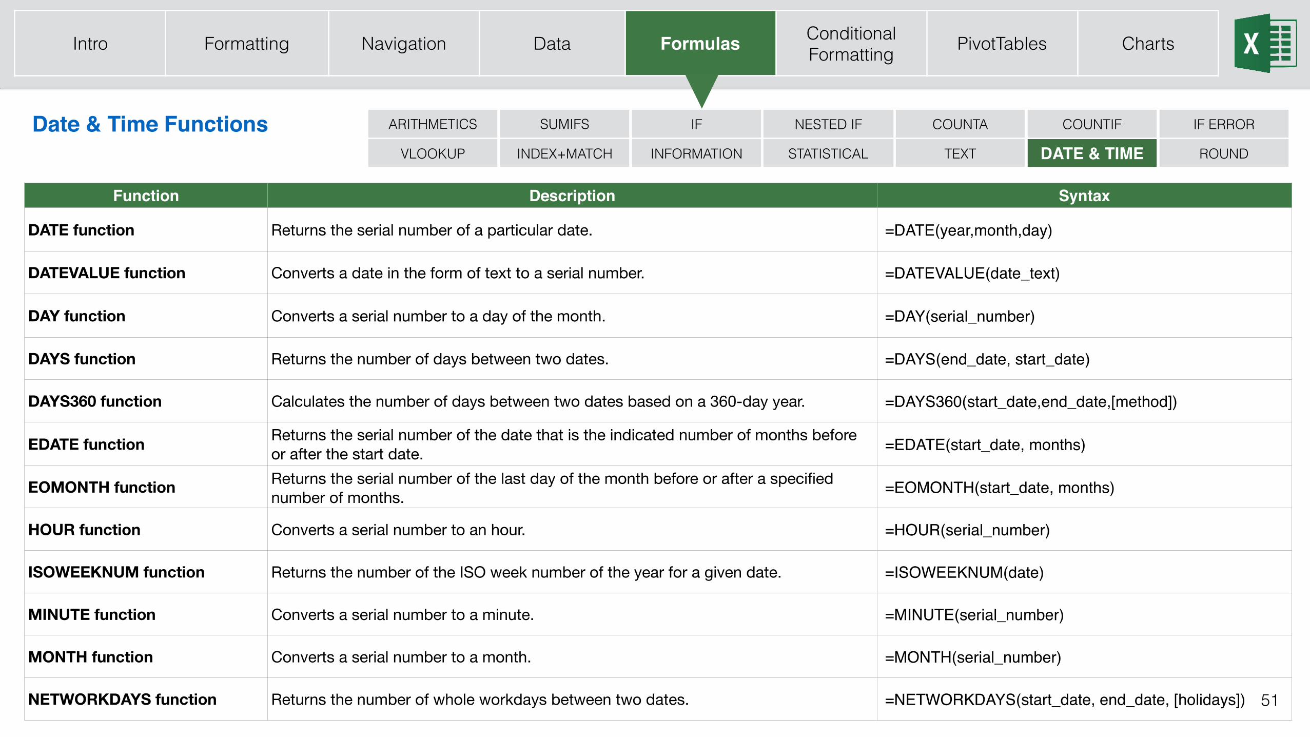
Function Description Syntax
DATE function Returns the serial number of a particular date. =DATE(year,month,day)
DATEVALUE function Converts a date in the form of text to a serial number. =DATEVALUE(date_text)
DAY function Converts a serial number to a day of the month. =DAY(serial_number)
DAYS function Returns the number of days between two dates. =DAYS(end_date, start_date)
DAYS360 function Calculates the number of days between two dates based on a 360-day year. =DAYS360(start_date,end_date,[method])
EDATE function Returns the serial number of the date that is the indicated number of months before or after the start date. =EDATE(start_date, months)
EOMONTH function Returns the serial number of the last day of the month before or after a specified number of months. =EOMONTH(start_date, months)
HOUR function Converts a serial number to an hour. =HOUR(serial_number)
ISOWEEKNUM function Returns the number of the ISO week number of the year for a given date. =ISOWEEKNUM(date)
MINUTE function Converts a serial number to a minute. =MINUTE(serial_number)
MONTH function Converts a serial number to a month. =MONTH(serial_number)
NETWORKDAYS function Returns the number of whole workdays between two dates. =NETWORKDAYS(start_date, end_date, [holidays])
INDEX+MATCH
COUNTAIF NESTED IFSUMIFSARITHMETICS
TEXTSTATISTICAL
IF ERROR
DATE & TIME
COUNTIF
VLOOKUP INFORMATION ROUND
Intro Formatting Navigation Data Formulas Conditional Formatting PivotTables Charts
52
Date & Time Functions
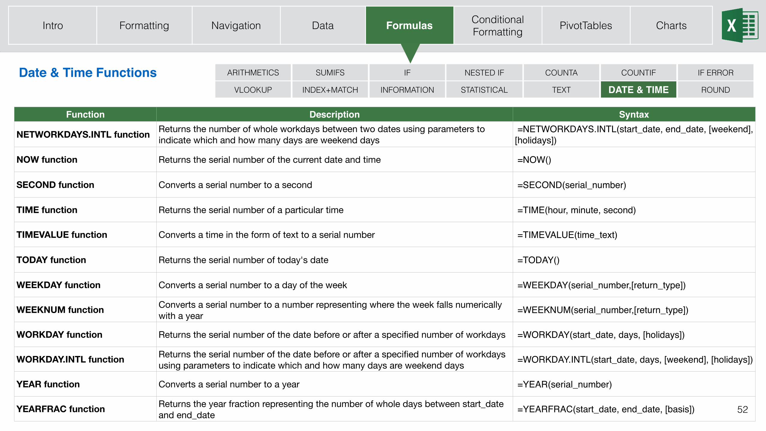
Function Description Syntax
NETWORKDAYS.INTL function Returns the number of whole workdays between two dates using parameters to indicate which and how many days are weekend days
=NETWORKDAYS.INTL(start_date, end_date, [weekend], [holidays])
NOW function Returns the serial number of the current date and time =NOW()
SECOND function Converts a serial number to a second =SECOND(serial_number)
TIME function Returns the serial number of a particular time =TIME(hour, minute, second)
TIMEVALUE function Converts a time in the form of text to a serial number =TIMEVALUE(time_text)
TODAY function Returns the serial number of today's date =TODAY()
WEEKDAY function Converts a serial number to a day of the week =WEEKDAY(serial_number,[return_type])
WEEKNUM function Converts a serial number to a number representing where the week falls numerically with a year =WEEKNUM(serial_number,[return_type])
WORKDAY function Returns the serial number of the date before or after a specified number of workdays =WORKDAY(start_date, days, [holidays])
WORKDAY.INTL function Returns the serial number of the date before or after a specified number of workdays using parameters to indicate which and how many days are weekend days =WORKDAY.INTL(start_date, days, [weekend], [holidays])
YEAR function Converts a serial number to a year =YEAR(serial_number)
YEARFRAC function Returns the year fraction representing the number of whole days between start_date and end_date =YEARFRAC(start_date, end_date, [basis])
INDEX+MATCH
COUNTAIF NESTED IFSUMIFSARITHMETICS
TEXTSTATISTICAL
IF ERROR
DATE & TIME
COUNTIF
VLOOKUP INFORMATION ROUND
Intro Formatting Navigation Data Formulas Conditional Formatting PivotTables Charts
53
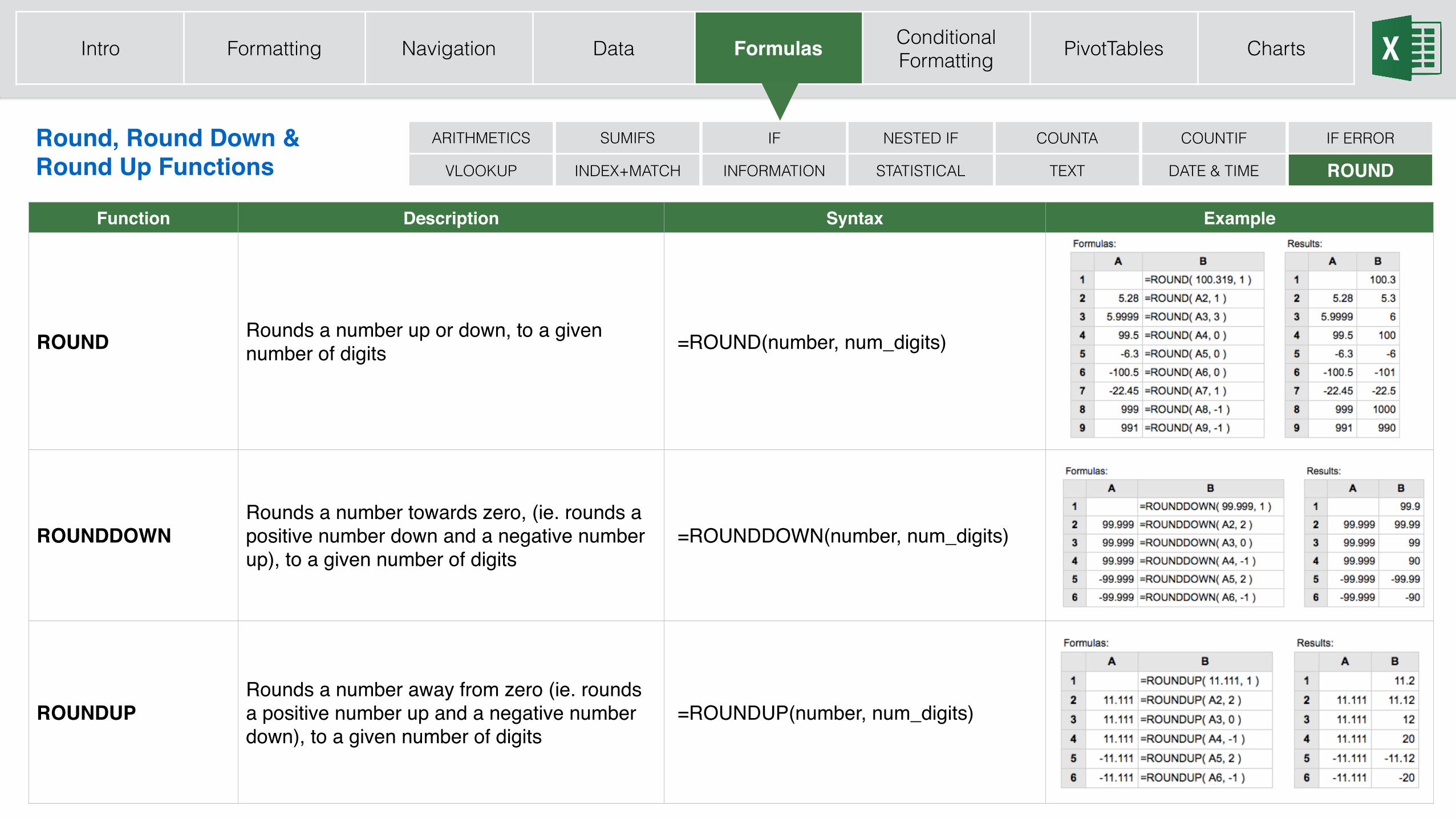
Round, Round Down & Round Up Functions INDEX+MATCH
COUNTAIF NESTED IFSUMIFSARITHMETICS
TEXTSTATISTICAL
IF ERROR
DATE & TIME
COUNTIF
VLOOKUP INFORMATION ROUND
Function Description Syntax Example
ROUND Rounds a number up or down, to a given number of digits =ROUND(number, num_digits)
ROUNDDOWNRounds a number towards zero, (ie. rounds a positive number down and a negative number up), to a given number of digits
=ROUNDDOWN(number, num_digits)
ROUNDUPRounds a number away from zero (ie. rounds a positive number up and a negative number down), to a given number of digits
=ROUNDUP(number, num_digits)
Intro Formatting Navigation Data Formulas Conditional Formatting PivotTables Charts
54
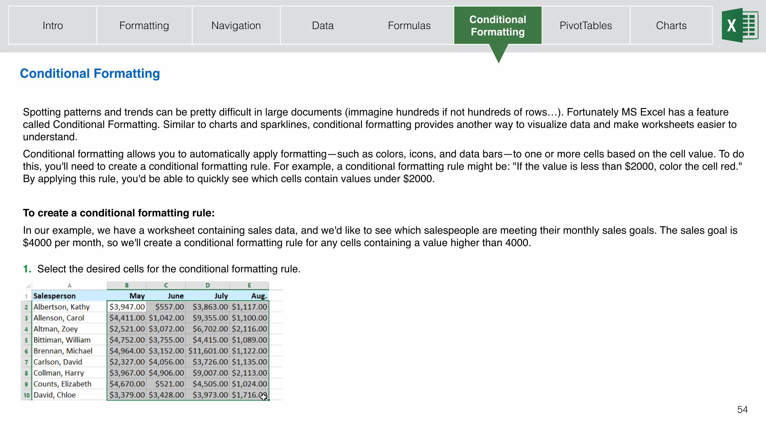
Conditional Formatting
Spotting patterns and trends can be pretty difficult in large documents (immagine hundreds if not hundreds of rows…). Fortunately MS Excel has a feature called Conditional Formatting. Similar to charts and sparklines, conditional formatting provides another way to visualize data and make worksheets easier to understand.Conditional formatting allows you to automatically apply formatting—such as colors, icons, and data bars—to one or more cells based on the cell value. To do this, you'll need to create a conditional formatting rule. For example, a conditional formatting rule might be: "If the value is less than $2000, color the cell red." By applying this rule, you'd be able to quickly see which cells contain values under $2000.
To create a conditional formatting rule:In our example, we have a worksheet containing sales data, and we'd like to see which salespeople are meeting their monthly sales goals. The sales goal is $4000 per month, so we'll create a conditional formatting rule for any cells containing a value higher than 4000.
1. Select the desired cells for the conditional formatting rule.
Intro Formatting Navigation Data Formulas ConditionalFormatting PivotTables Charts
55
Conditional Formatting
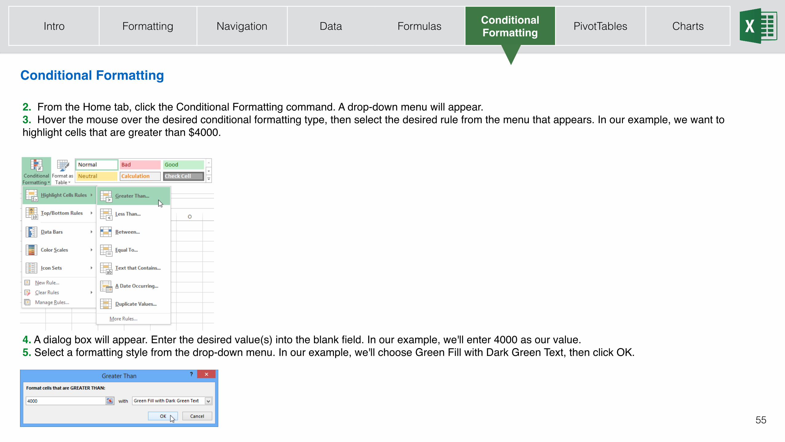
4. A dialog box will appear. Enter the desired value(s) into the blank field. In our example, we'll enter 4000 as our value.5. Select a formatting style from the drop-down menu. In our example, we'll choose Green Fill with Dark Green Text, then click OK.
2. From the Home tab, click the Conditional Formatting command. A drop-down menu will appear.3. Hover the mouse over the desired conditional formatting type, then select the desired rule from the menu that appears. In our example, we want to highlight cells that are greater than $4000.
Intro Formatting Navigation Data Formulas ConditionalFormatting PivotTables Charts
56
Conditional Formatting
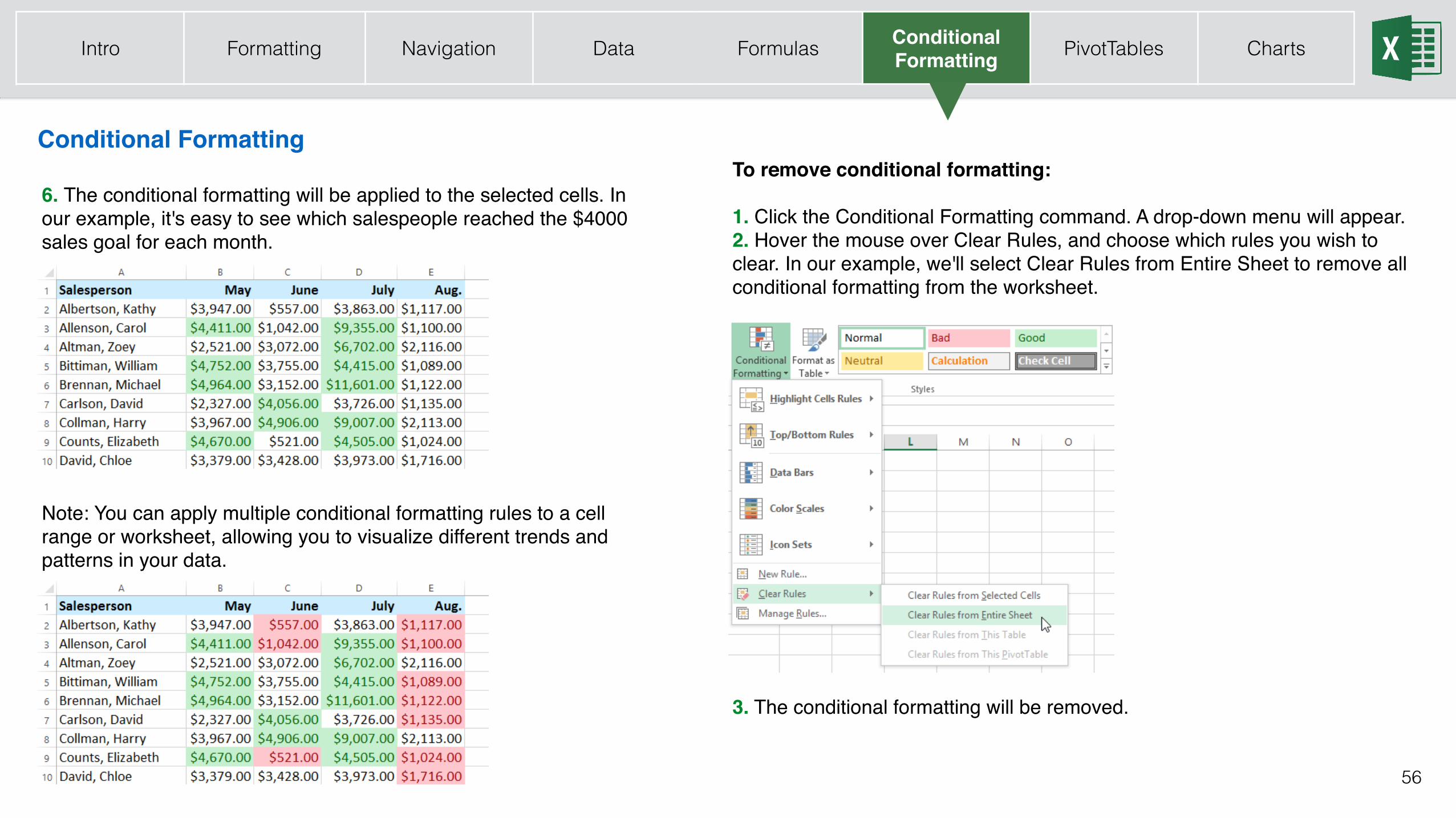
Note: You can apply multiple conditional formatting rules to a cell range or worksheet, allowing you to visualize different trends and patterns in your data.
To remove conditional formatting:
1. Click the Conditional Formatting command. A drop-down menu will appear.2. Hover the mouse over Clear Rules, and choose which rules you wish to clear. In our example, we'll select Clear Rules from Entire Sheet to remove all conditional formatting from the worksheet.
6. The conditional formatting will be applied to the selected cells. In our example, it's easy to see which salespeople reached the $4000 sales goal for each month.
3. The conditional formatting will be removed.
Intro Formatting Navigation Data Formulas ConditionalFormatting PivotTables Charts
57
PivotTables
Intro Formatting Navigation Data Formulas Conditional Formatting PivotTables Charts
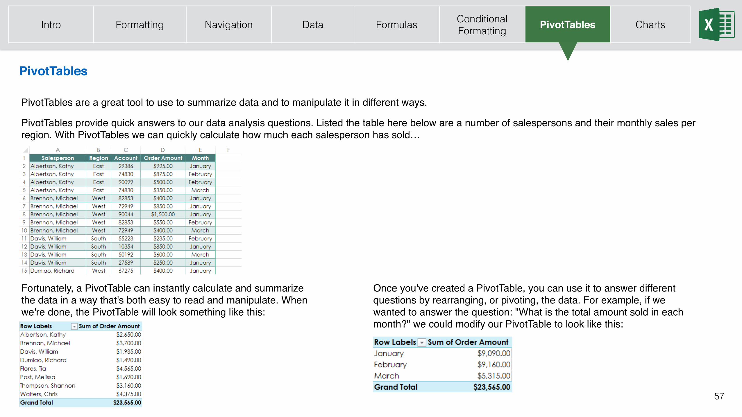
PivotTables are a great tool to use to summarize data and to manipulate it in different ways.
PivotTables provide quick answers to our data analysis questions. Listed the table here below are a number of salespersons and their monthly sales per region. With PivotTables we can quickly calculate how much each salesperson has sold…
Fortunately, a PivotTable can instantly calculate and summarize the data in a way that's both easy to read and manipulate. When we're done, the PivotTable will look something like this:
Once you've created a PivotTable, you can use it to answer different questions by rearranging, or pivoting, the data. For example, if we wanted to answer the question: "What is the total amount sold in each month?" we could modify our PivotTable to look like this:
58
Create a Pivot Table
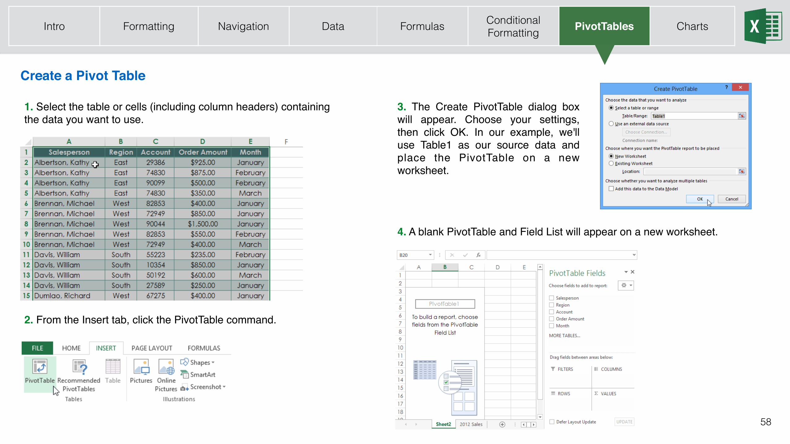
1. Select the table or cells (including column headers) containing the data you want to use.
2. From the Insert tab, click the PivotTable command.
3. The Create PivotTable dialog box will appear. Choose your settings, then click OK. In our example, we'll use Table1 as our source data and place the PivotTable on a new worksheet.
4. A blank PivotTable and Field List will appear on a new worksheet.
Intro Formatting Navigation Data Formulas Conditional Formatting PivotTables Charts
59
Create a Pivot Table
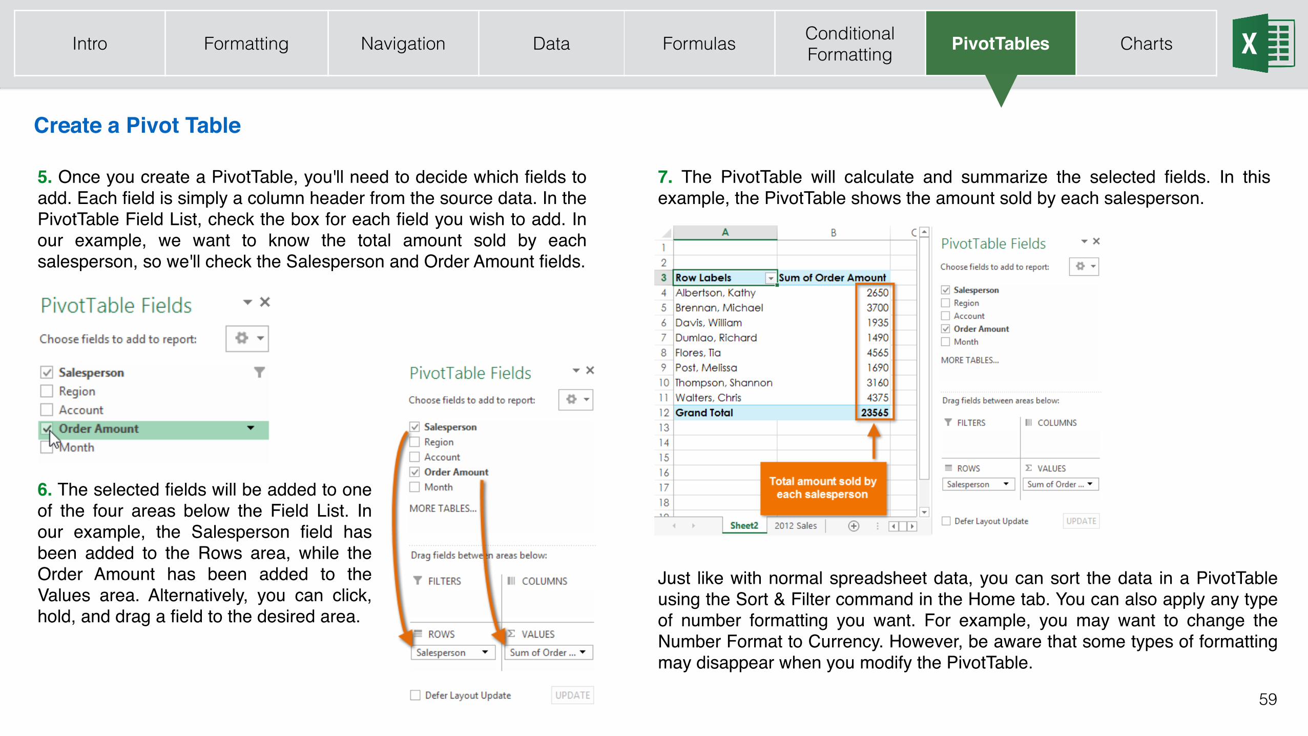
5. Once you create a PivotTable, you'll need to decide which fields to add. Each field is simply a column header from the source data. In the PivotTable Field List, check the box for each field you wish to add. In our example, we want to know the total amount sold by each salesperson, so we'll check the Salesperson and Order Amount fields.
6. The selected fields will be added to one of the four areas below the Field List. In our example, the Salesperson field has been added to the Rows area, while the Order Amount has been added to the Values area. Alternatively, you can click, hold, and drag a field to the desired area.
7. The PivotTable will calculate and summarize the selected fields. In this example, the PivotTable shows the amount sold by each salesperson.
Just like with normal spreadsheet data, you can sort the data in a PivotTable using the Sort & Filter command in the Home tab. You can also apply any type of number formatting you want. For example, you may want to change the Number Format to Currency. However, be aware that some types of formatting may disappear when you modify the PivotTable.
Intro Formatting Navigation Data Formulas Conditional Formatting PivotTables Charts
60
Pivoting data
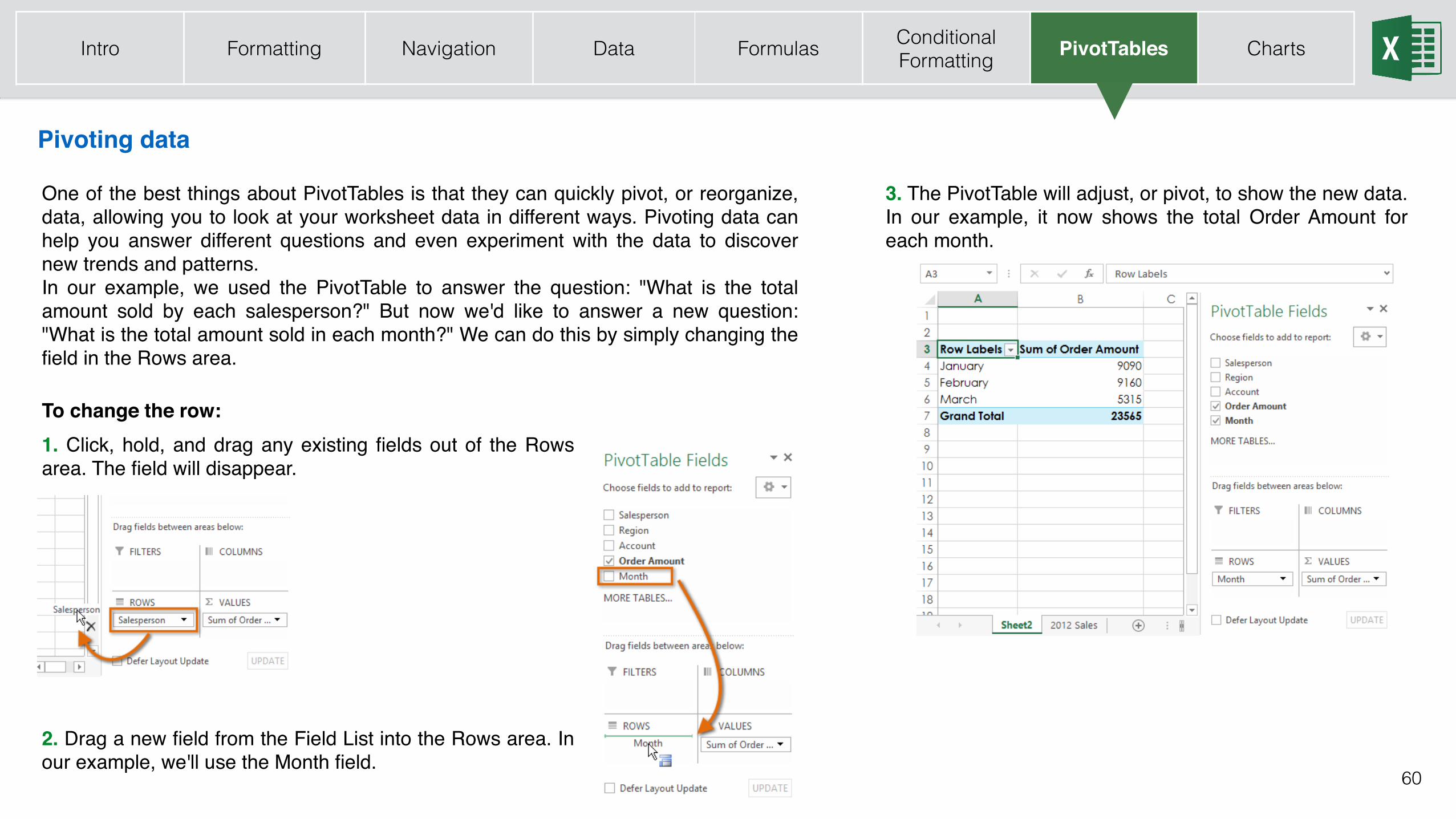
One of the best things about PivotTables is that they can quickly pivot, or reorganize, data, allowing you to look at your worksheet data in different ways. Pivoting data can help you answer different questions and even experiment with the data to discover new trends and patterns.In our example, we used the PivotTable to answer the question: "What is the total amount sold by each salesperson?" But now we'd like to answer a new question: "What is the total amount sold in each month?" We can do this by simply changing the field in the Rows area.
To change the row:1. Click, hold, and drag any existing fields out of the Rows area. The field will disappear.
2. Drag a new field from the Field List into the Rows area. In our example, we'll use the Month field.
3. The PivotTable will adjust, or pivot, to show the new data. In our example, it now shows the total Order Amount for each month.
Intro Formatting Navigation Data Formulas Conditional Formatting PivotTables Charts
61
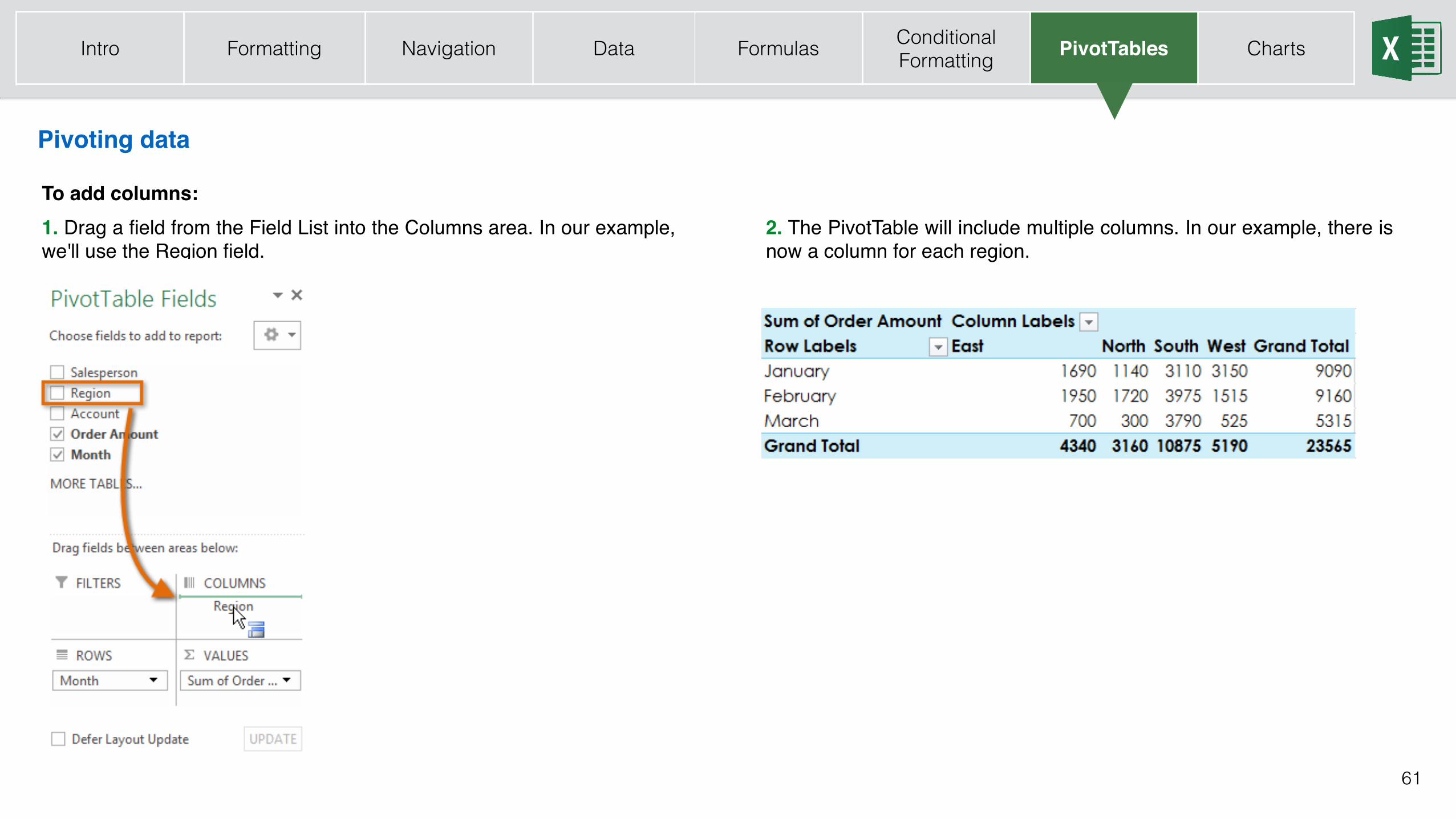
Pivoting data
To add columns:1. Drag a field from the Field List into the Columns area. In our example, we'll use the Region field.
2. The PivotTable will include multiple columns. In our example, there is now a column for each region.
Intro Formatting Navigation Data Formulas Conditional Formatting PivotTables Charts
62
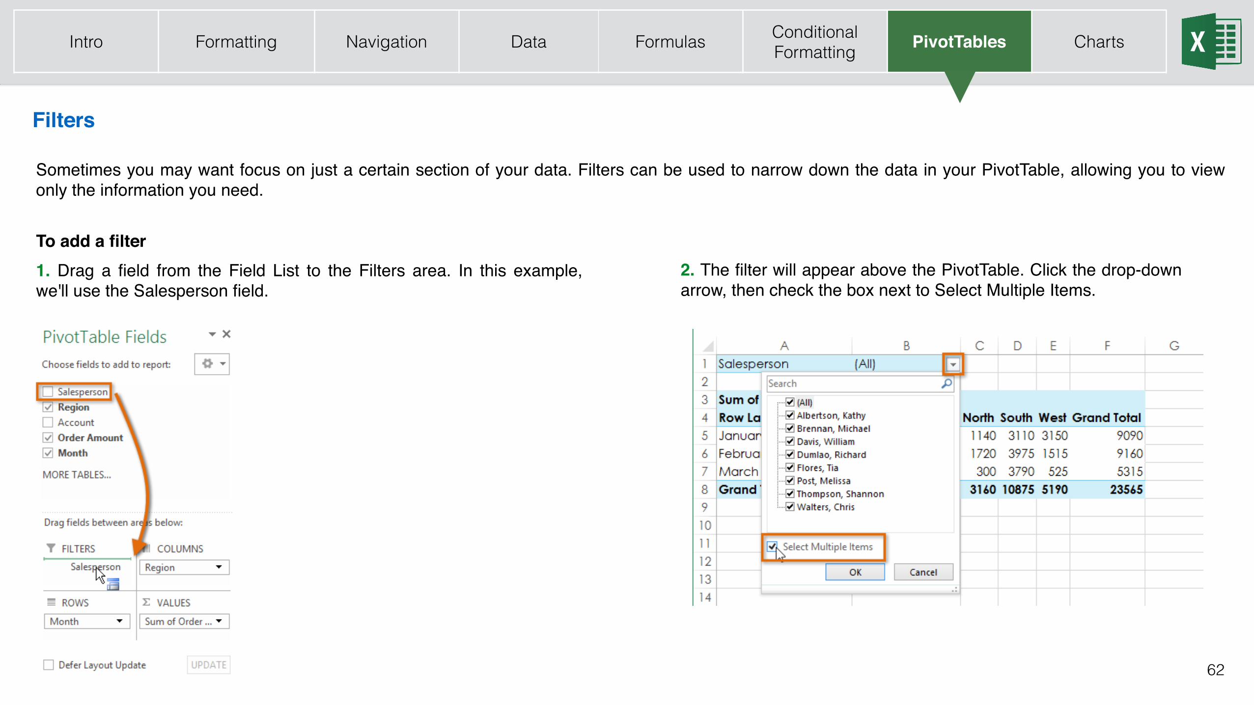
Filters
Sometimes you may want focus on just a certain section of your data. Filters can be used to narrow down the data in your PivotTable, allowing you to view only the information you need.
To add a filter1. Drag a field from the Field List to the Filters area. In this example, we'll use the Salesperson field.
2. The filter will appear above the PivotTable. Click the drop-down arrow, then check the box next to Select Multiple Items.
Intro Formatting Navigation Data Formulas Conditional Formatting PivotTables Charts
63
Filters
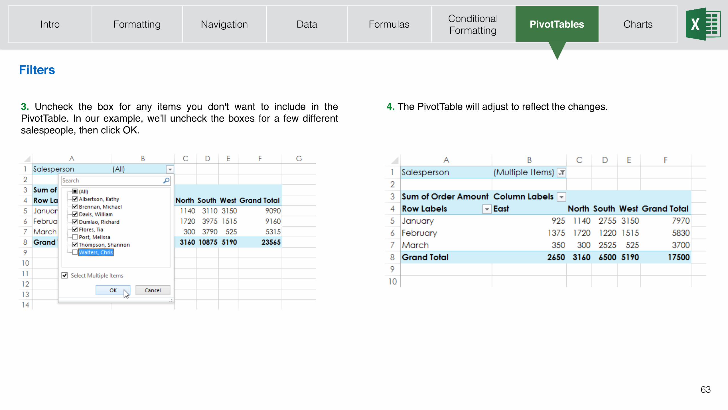
3. Uncheck the box for any items you don't want to include in the PivotTable. In our example, we'll uncheck the boxes for a few different salespeople, then click OK.
4. The PivotTable will adjust to reflect the changes.
Intro Formatting Navigation Data Formulas Conditional Formatting PivotTables Charts
64
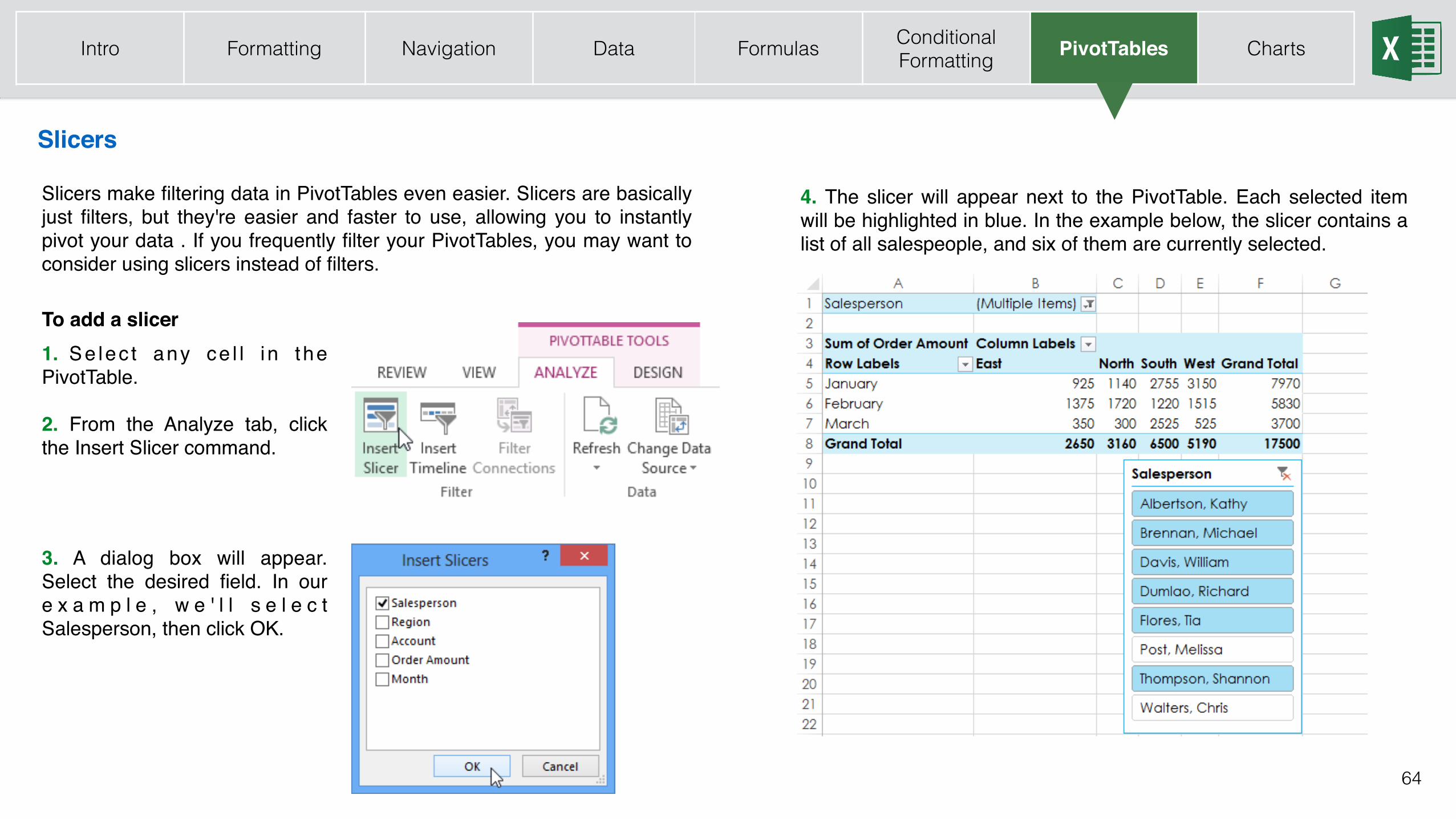
Slicers
4. The slicer will appear next to the PivotTable. Each selected item will be highlighted in blue. In the example below, the slicer contains a list of all salespeople, and six of them are currently selected.
Slicers make filtering data in PivotTables even easier. Slicers are basically just filters, but they're easier and faster to use, allowing you to instantly pivot your data . If you frequently filter your PivotTables, you may want to consider using slicers instead of filters.
To add a slicer1. Se lec t any ce l l i n the PivotTable.
2. From the Analyze tab, click the Insert Slicer command.
3. A dialog box will appear. Select the desired field. In our e x a m p l e , w e ' l l s e l e c t Salesperson, then click OK.
Intro Formatting Navigation Data Formulas Conditional Formatting PivotTables Charts
65
Slicers
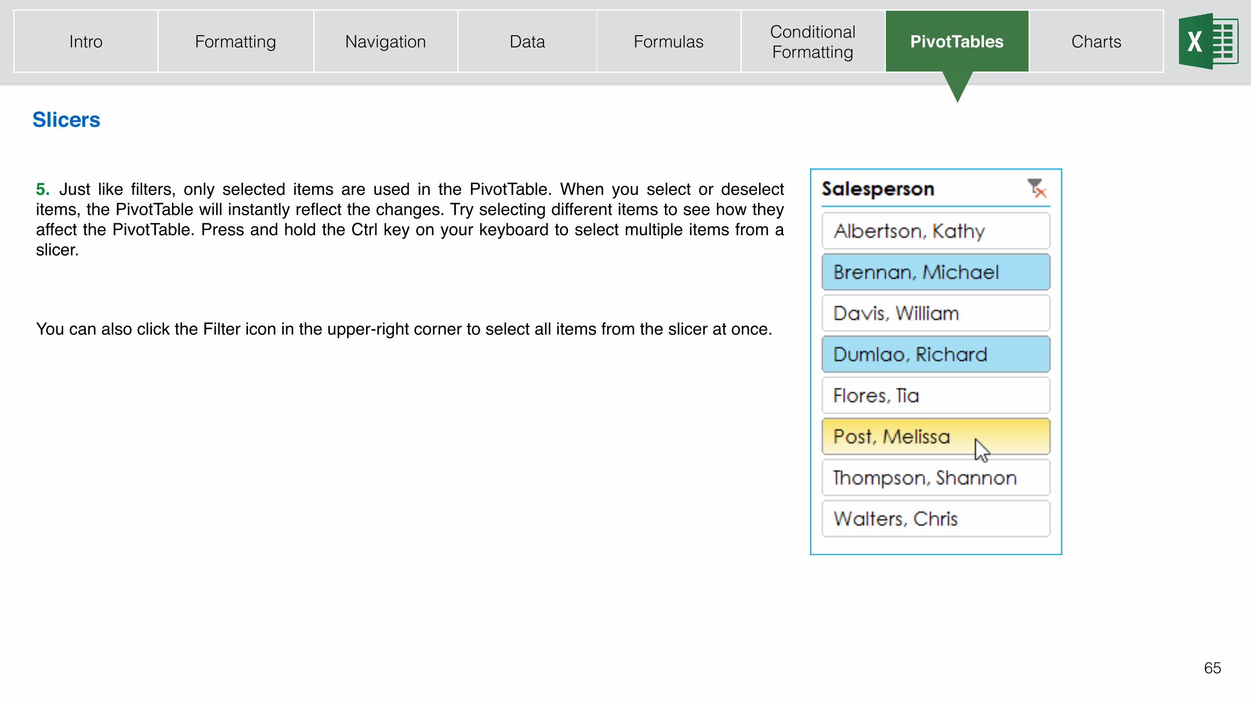
5. Just like filters, only selected items are used in the PivotTable. When you select or deselect items, the PivotTable will instantly reflect the changes. Try selecting different items to see how they affect the PivotTable. Press and hold the Ctrl key on your keyboard to select multiple items from a slicer.
You can also click the Filter icon in the upper-right corner to select all items from the slicer at once.
Intro Formatting Navigation Data Formulas Conditional Formatting PivotTables Charts
66
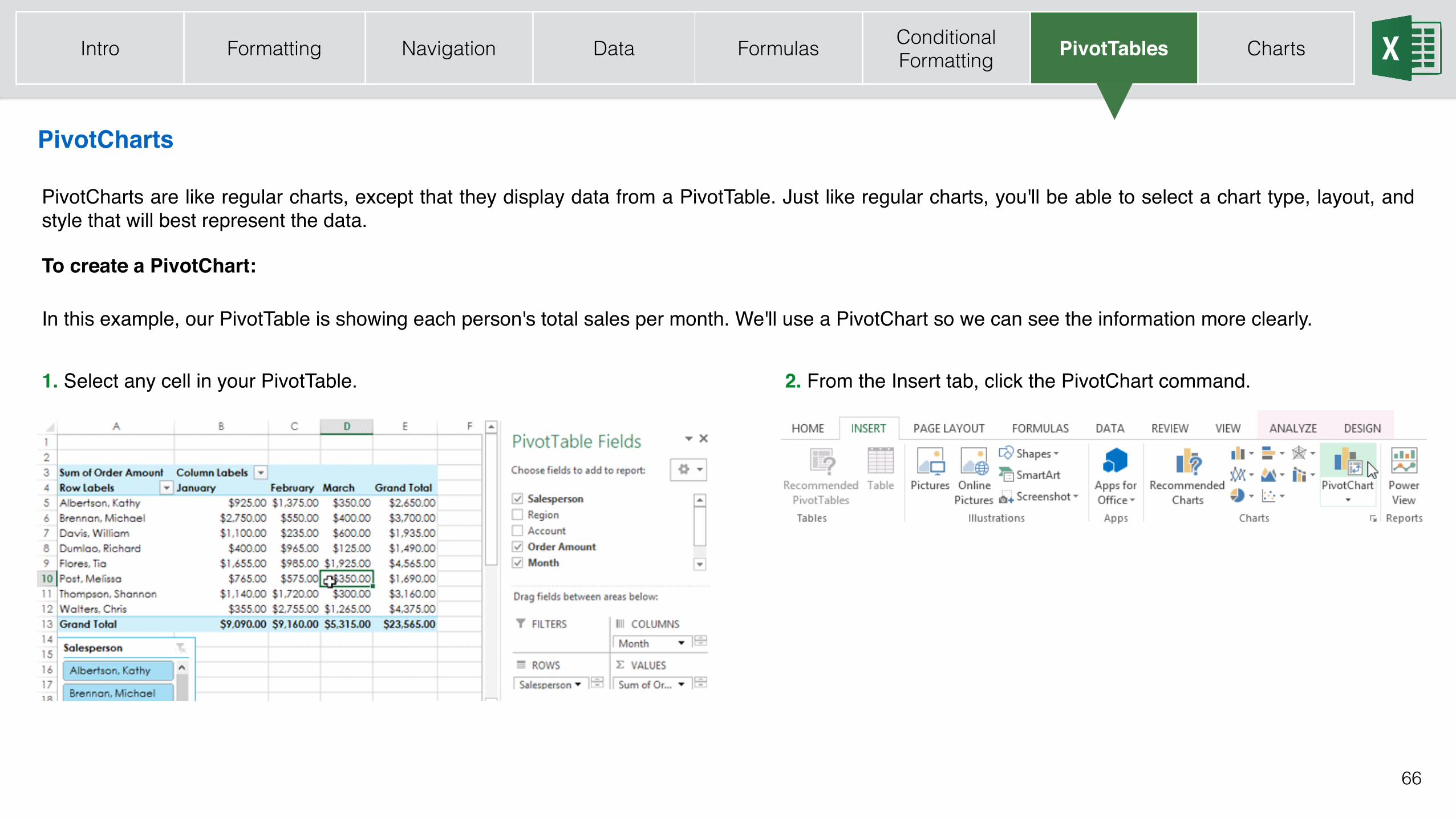
PivotCharts
PivotCharts are like regular charts, except that they display data from a PivotTable. Just like regular charts, you'll be able to select a chart type, layout, and style that will best represent the data.
To create a PivotChart:
In this example, our PivotTable is showing each person's total sales per month. We'll use a PivotChart so we can see the information more clearly.
1. Select any cell in your PivotTable. 2. From the Insert tab, click the PivotChart command.
Intro Formatting Navigation Data Formulas Conditional Formatting PivotTables Charts
67
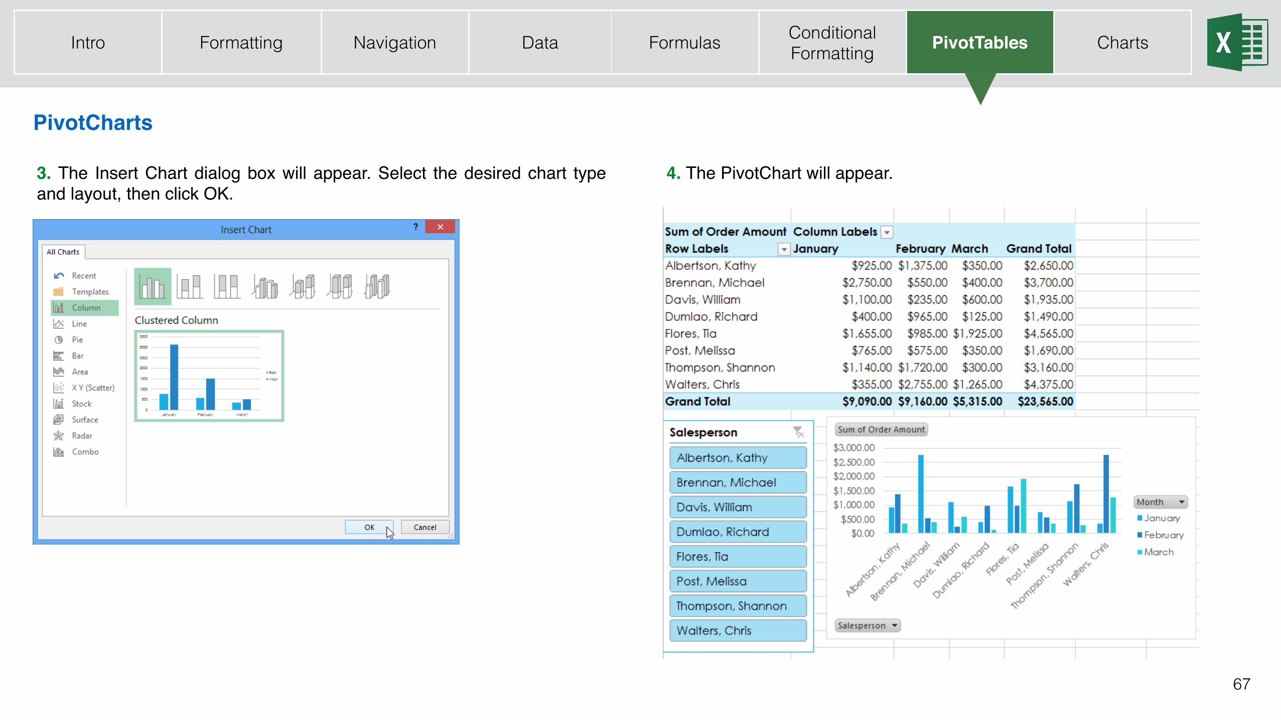
PivotCharts
3. The Insert Chart dialog box will appear. Select the desired chart type and layout, then click OK.
4. The PivotChart will appear.
Intro Formatting Navigation Data Formulas Conditional Formatting PivotTables Charts
68
PivotCharts
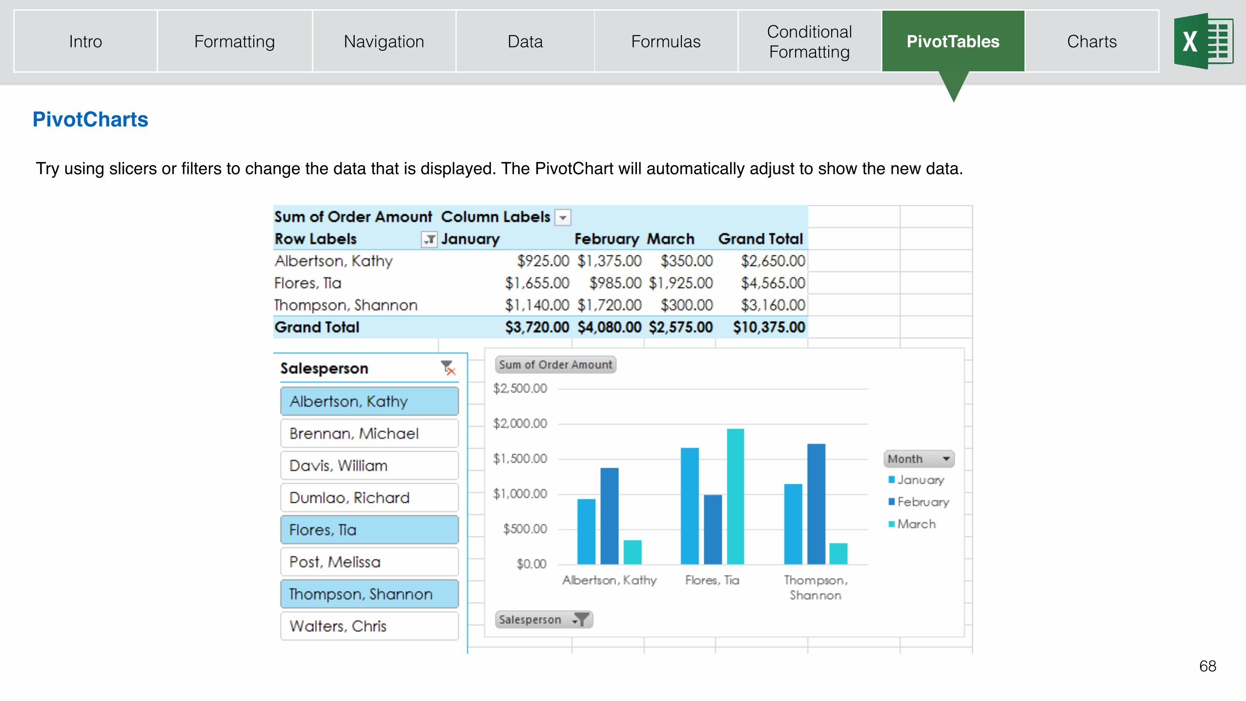
Try using slicers or filters to change the data that is displayed. The PivotChart will automatically adjust to show the new data.
Intro Formatting Navigation Data Formulas Conditional Formatting PivotTables Charts
69
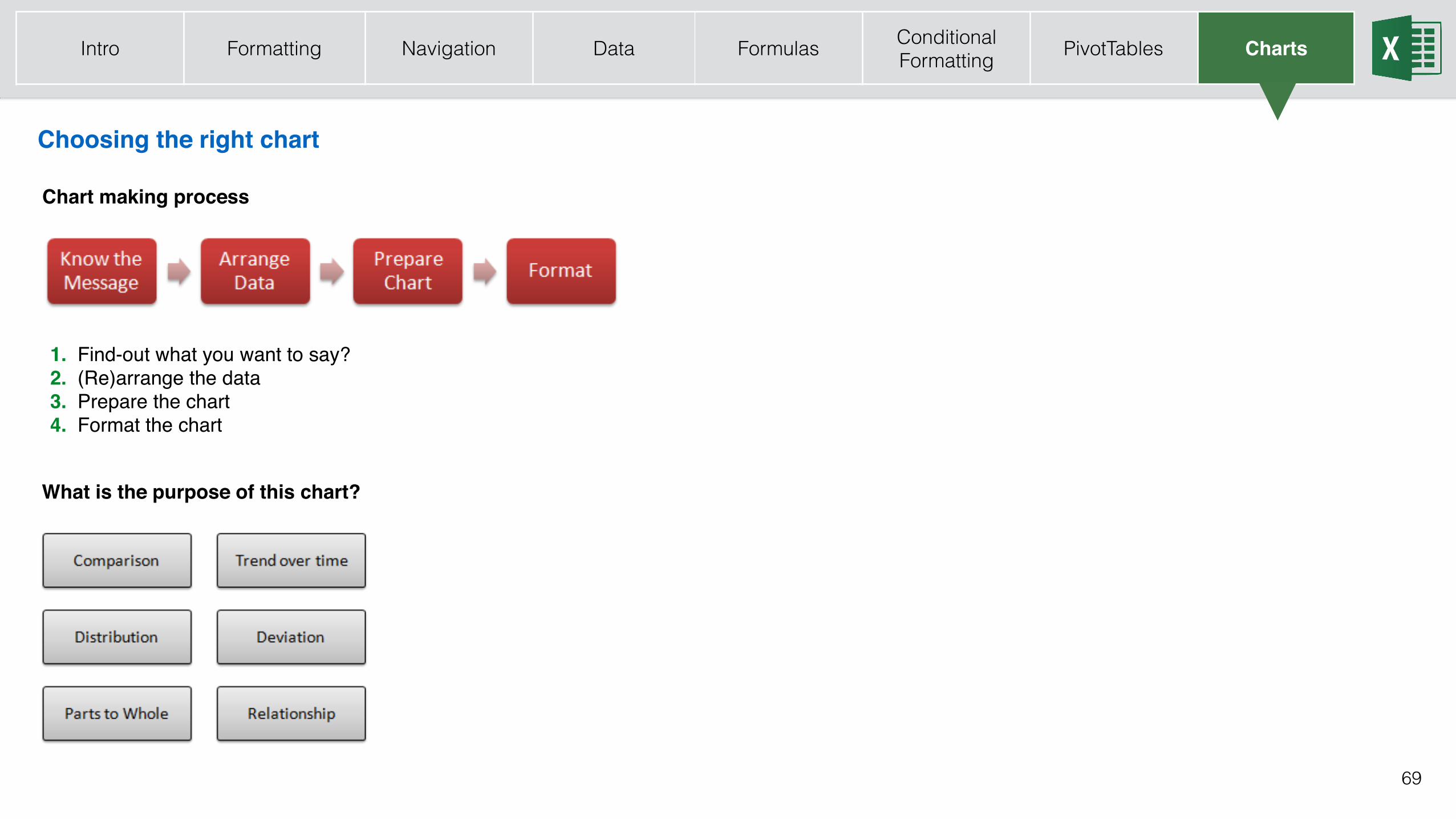
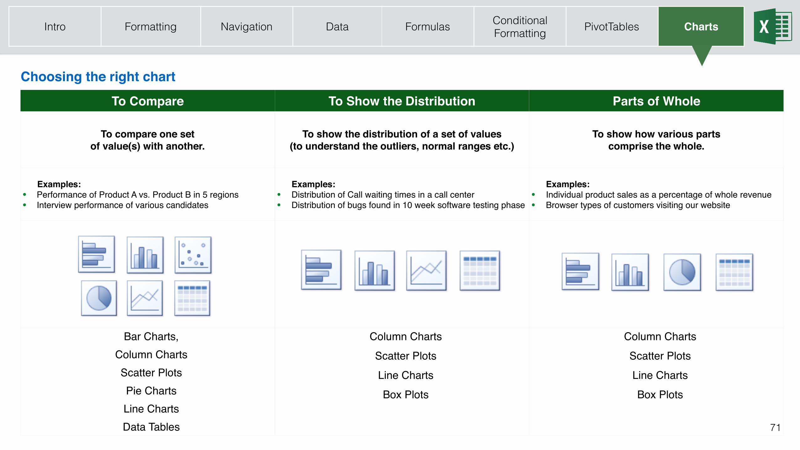
Choosing the right chart
Intro Formatting Navigation Data Formulas Conditional Formatting PivotTables Charts
1. Find-out what you want to say? 2. (Re)arrange the data 3. Prepare the chart 4. Format the chart
What is the purpose of this chart?
Chart making process

70
Intro Formatting Navigation Data Formulas Conditional Formatting PivotTables Charts
71
Choosing the right chart
Intro Formatting Navigation Data Formulas Conditional Formatting PivotTables Charts
To Compare To Show the Distribution Parts of Whole
To compare one set of value(s) with another.
To show the distribution of a set of values (to understand the outliers, normal ranges etc.)
To show how various parts comprise the whole.
Examples:• Performance of Product A vs. Product B in 5 regions• Interview performance of various candidates
Examples:• Distribution of Call waiting times in a call center• Distribution of bugs found in 10 week software testing phase
Examples:• Individual product sales as a percentage of whole revenue• Browser types of customers visiting our website
Bar Charts,Column ChartsScatter PlotsPie ChartsLine ChartsData Tables
Column ChartsScatter PlotsLine ChartsBox Plots
Column ChartsScatter PlotsLine ChartsBox Plots
t
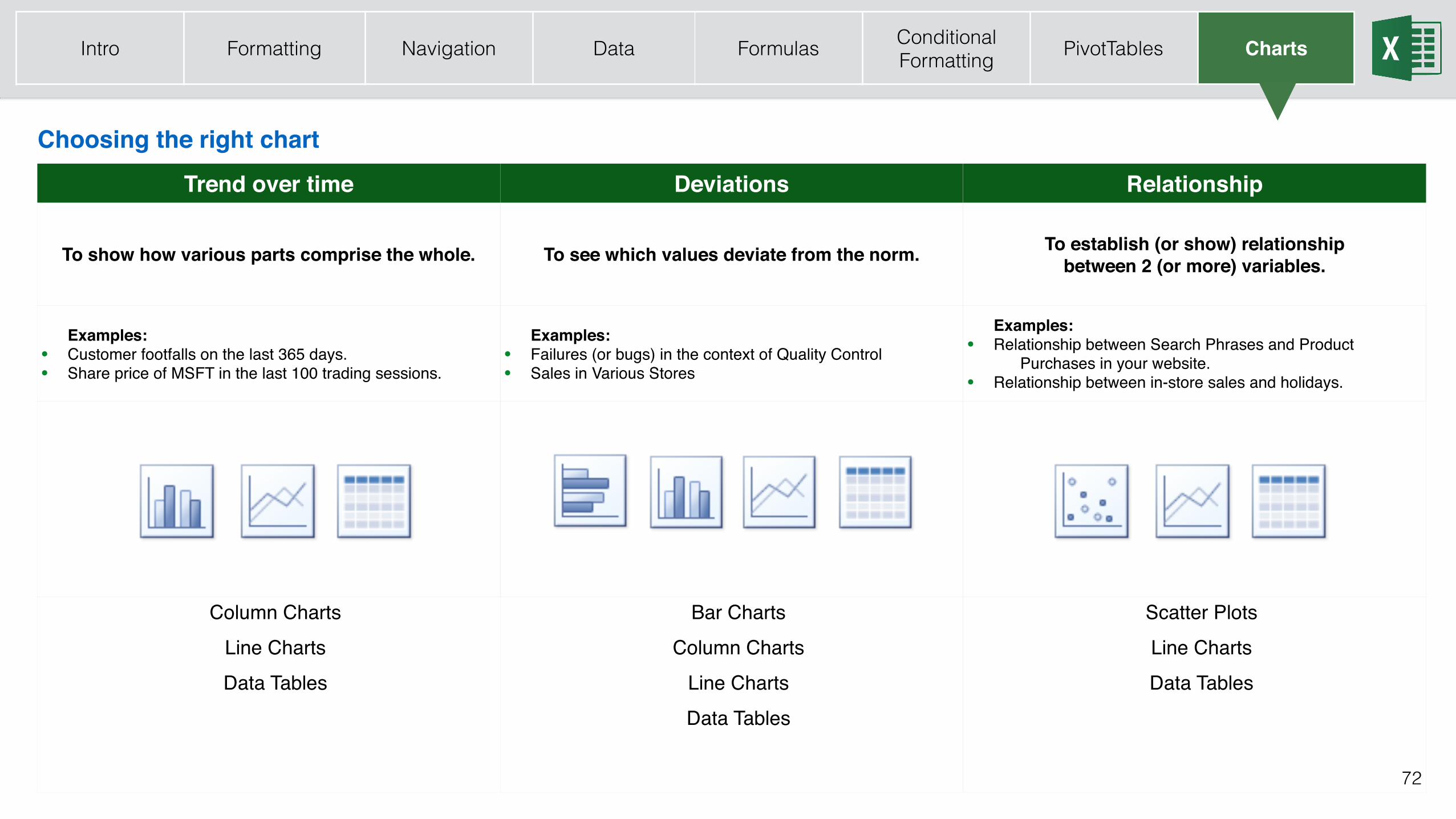
72
Choosing the right chart
Intro Formatting Navigation Data Formulas Conditional Formatting PivotTables Charts
Trend over time Deviations Relationship
To show how various parts comprise the whole. To see which values deviate from the norm. To establish (or show) relationship between 2 (or more) variables.
Examples:• Customer footfalls on the last 365 days.• Share price of MSFT in the last 100 trading sessions.
Examples:• Failures (or bugs) in the context of Quality Control• Sales in Various Stores
Examples:• Relationship between Search Phrases and Product
Purchases in your website.• Relationship between in-store sales and holidays.
Column ChartsLine ChartsData Tables
Bar ChartsColumn Charts
Line ChartsData Tables
Scatter PlotsLine ChartsData Tables
t
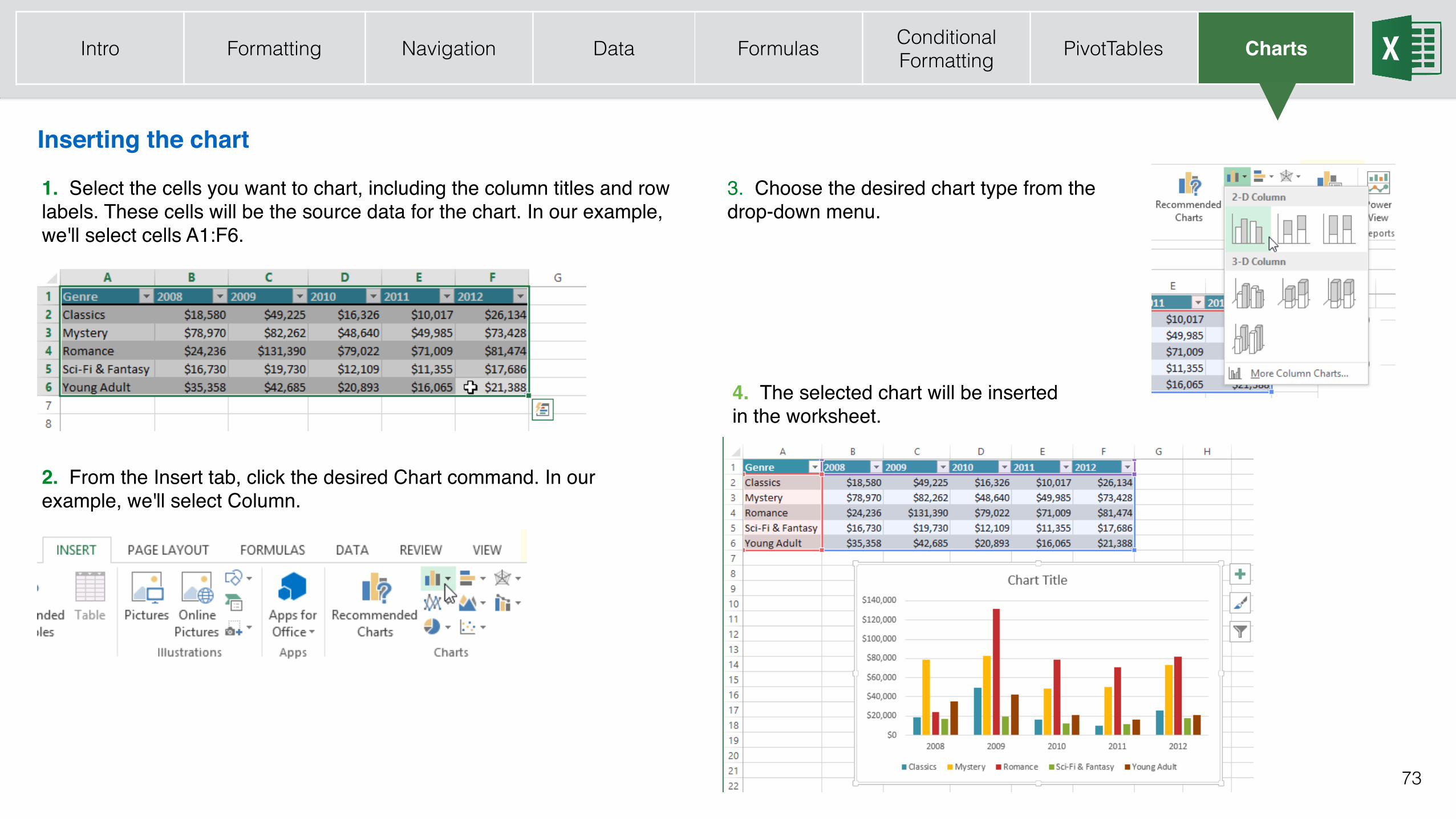
73
Inserting the chart
Intro Formatting Navigation Data Formulas Conditional Formatting PivotTables Charts
1. Select the cells you want to chart, including the column titles and row labels. These cells will be the source data for the chart. In our example, we'll select cells A1:F6.
2. From the Insert tab, click the desired Chart command. In our example, we'll select Column.
3. Choose the desired chart type from the drop-down menu.
4. The selected chart will be inserted in the worksheet.
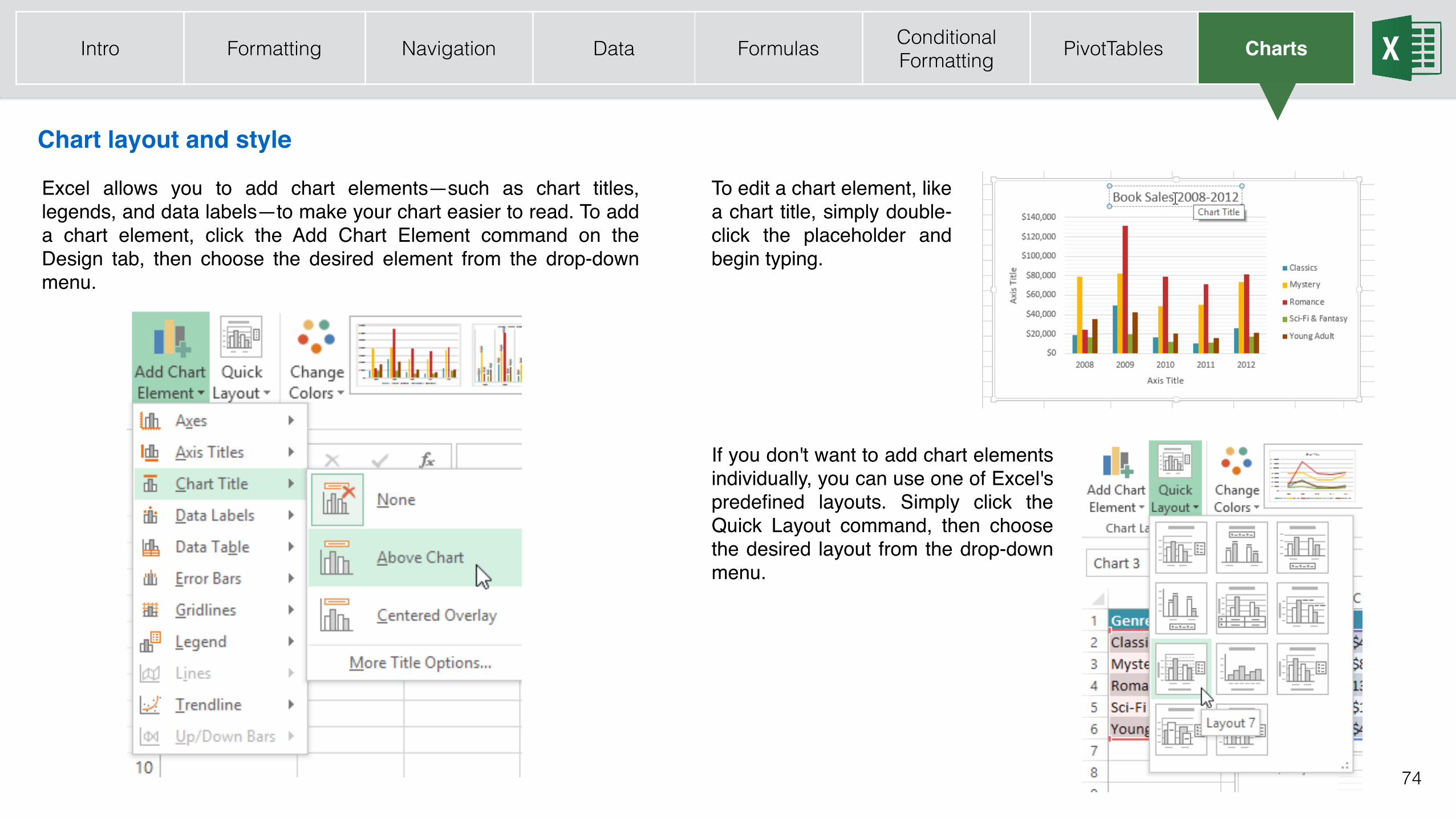
74
Chart layout and style
Intro Formatting Navigation Data Formulas Conditional Formatting PivotTables Charts
Excel allows you to add chart elements—such as chart titles, legends, and data labels—to make your chart easier to read. To add a chart element, click the Add Chart Element command on the Design tab, then choose the desired element from the drop-down menu.
To edit a chart element, like a chart title, simply double-click the placeholder and begin typing.
If you don't want to add chart elements individually, you can use one of Excel's predefined layouts. Simply click the Quick Layout command, then choose the desired layout from the drop-down menu.
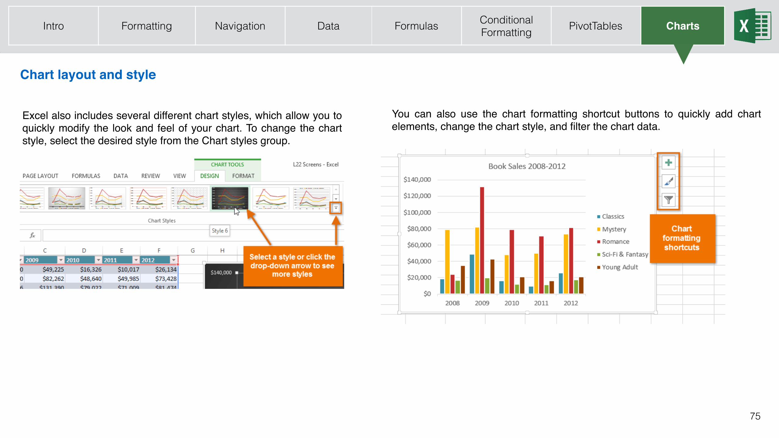
75
Chart layout and style
Intro Formatting Navigation Data Formulas Conditional Formatting PivotTables Charts
Excel also includes several different chart styles, which allow you to quickly modify the look and feel of your chart. To change the chart style, select the desired style from the Chart styles group.
You can also use the chart formatting shortcut buttons to quickly add chart elements, change the chart style, and filter the chart data.