Recent Advances in CPLEX 12.6.1

Decision OptimizationDecision Optimization

Recent Advances in IBM ILOG CPLEX Optimization Studio

Andrea TramontaniCPLEX Optimization, IBM

© 2013 IBM Corporation

CPLEX 12.6.1 performance improvements– Summary– Presolve– Branching

Local implied bound cuts– Global vs. local implied bound cuts– An interesting use case

CPLEX 12.6.1 features– CPLEX Python API: now includes support for Python 3– New parameter to control product linearization in MIQP– Opportunistic distributed memory MIP

2

Outline


Date: 5 November 2014Testset: 3147 models (1792 in ≥ 10sec, 1554 in ≥ 100sec, 1384 in ≥ 1000sec)Machine: Intel X5650 @ 2.67GHz, 24 GB RAM, 12 threads (deterministic since CPLEX 11.0)Timelimit: 10,000 sec

3

MIP Performance Evolution in CPLEX

3

≥≥ 10 sec10 sec

≥≥ 100 sec100 sec

≥≥ 1000 sec1000 sec


Deterministic parallel MILP (12 threads)Deterministic parallel MILP (12 threads)

4

CPLEX 12.6.0 vs. CPLEX 12.6.1: MIP Performance Improvement

4

1.00

0.94

1.00

0.91

1.00

0.86

0

0.1

0.2

0.3

0.4

0.5

0.6

0.7

0.8

0.9

1

>1s >10s >100s

CPLEX 12.6.0

CPLEX 12.6.1

19751975modelsmodels


619619modelsmodels

Time limits:40 / 28

Date: 5 November 2014Testset: MILP: 4134 modelsMachine: Intel X5650 @ 2.67GHz, 24 GB RAM, 12 threads, deterministicTimelimit: 10,000 sec

1.06x1.06x 1.10x1.10x 1.16x1.16x

© 2013 IBM Corporation5

CPLEX 12.6.0 vs. CPLEX 12.6.1: MIP Performance Improvement (Cont. d)

5

1.0

0

0.7

8

1.0

0

0.6

0

0

0.1

0.2

0.3

0.4

0.5

0.6

0.7

0.8

0.9

1

>0s >1s

CPLEX 12.6.0

CPLEX 12.6.1

251 models251 models

Time limits:11 / 4

1.28x1.28x 1.67x1.67x Convex MIQPConvex MIQP


1.0

0

0.8

1

1.0

0

0.7

2

0

0.1

0.2

0.3

0.4

0.5

0.6

0.7

0.8

0.9

1

>0s >1s

CPLEX 12.6.0

CPLEX 12.6.1


Time limits:1 / 1

1.23x1.23x 1.39x1.39x Convex MIQCPConvex MIQCP


Date: 5 November 2014Testset: Convex MIQP: 335 models, Convex MIQCP: 190 models, Machine: Intel X5650 @ 2.67GHz, 24 GB RAM, 12 threads, deterministicTimelimit: 10,000 sec


CPLEX 12.6.0 vs. CPLEX 12.6.1: MIP Performance Improvement (Cont. d, 2)

6

1.00

0.90

1.00

0.75

0

0.1

0.2

0.3

0.4

0.5

0.6

0.7

0.8

0.9

1

>0s >1s

CPLEX 12.6.0

CPLEX 12.6.1


Time limits:2 / 2

1.11x1.11x 1.33x1.33xNon Convex (MI)QPNon Convex (MI)QP


The test set includes 308 QPs and 286 MIQPs– Same algorithmic framework (spatial branch-and-bound)– Very similar improvements on QPs and MIQPs

Date: 5 November 2014Testset: Non Convex QP: 308 models, Non Convex MIQP: 286 modelsMachine: Intel X5650 @ 2.67GHz, 24 GB RAM, 12 threads, deterministicTimelimit: 10,000 sec


Cuts– Different separation strategies in parallel cut loop– Improvements in MIR cut aggregator

• Better handling of mixed integer models with general integer variables

Presolve– Constraint disaggregation– Propagation of quadratic objective function and constraints in node presolve

Branching– Improvements in branching rule tie breaking– Improvements in reliability branching

Other improvements– General improvements on dynamic search (mostly for MIQP)– General improvements in global solver for non-convex (MI)QP– Improvements on QP simplex

7

Performance Improvements in CPLEX 12.6.1 – Summary


Disaggregate constraints that can be dominated by a set of “implied bound constraints”– Example (trivial case):

The implications x = 1 --> yi ≤ 0 (i = 1, 2, …, N) dominate y1 + y2 + … + yN ≤ N x

System (1) can be tightened as

8

Presolve: constraint disaggregation

y1 + y2 + … + yN ≤ N x0 ≤ yi ≤ 1, i = 1, 2, …, N (1)x in {0, 1}

yi ≤ x, i = 1, 2, …, N0 ≤ yi ≤ 1, i = 1, 2, …, N (2)x in {0, 1}


Trade off between tightening and number of non zeros added– The larger is N, the larger is the expected tightening– Disaggregating a constraint of length N implies adding N-1 rows and N-1 non

zeros

Applied rather conservatively– Only 16% of hard models (≥ 100 sec) affected– 10-14% speed-up on the affected models

9

Presolve: constraint disaggregation (Cont. d)


Given a quadratic constraint with bounded variables:

Relax the constraint in the box [L , U] exposing a given variable xj :

Then compute the two roots R- and R+ (with R- < R+), i.e. the solutions of

Case 1: qj > 0

– R- and R+ are valid bounds for xj --> Lj = max {Lj, R-}, Uj = min {Uj, R

+}

Case 2: qj < 0

– R- < Lj --> R+ is a valid lower bound for xj --> Lj = max {Lj, R+}

– R+ > Uj --> R- is a valid upper bound for xj --> Uj = min {Uj, R-}

– R- < Lj ≤ Uj < R+ --> the problem is infeasible

10

Presolve: propagation of quadratic objective and constraints

0.5 xTQ x + aT x + b ≤ 0,L ≤ x ≤ U

0.5 qj xj2 + cj

xj + d ≤ 0,Lj ≤ xj ≤ Uj

0.5 qj xj2 + cj

xj + d = 0


Presolve: propagation of quadratic objective and constraints (Cont. d)

Propagation in root presolve– Speed-up is 0%

Propagation in node presolve:– Convex MIQP

• 16% of models affected• 1-4% speed-up on the affected models

– Convex MIQCP• 57% of models affected• 12-20% speed-up on the affected models

– Non Convex MIQP• 27% of models affected• 6-7% speed-up on the affected models

Globally valid implications


CPLEX branching is mostly branching on single fractional variables

Default strategy is Hybrid branching (Achterberg and Berthold, 2009):– Reliability branching (Achterberg, Koch and Martin, 2005)

• Generalization of pseudo cost with strong branching initialization (Linderoth and Savelsbergh, 1999)

• Clever combination of strong branching and pseudo cost branching• Among fractional variables, identify the ones with unreliable pseudo cost• Apply strong branching to some (possibly, all) unreliable candidates to update their

pseudo costs and make them reliable• Apply pseudo cost branching to all candidates with reliable pseudo cost

– Conflict scores• Prefer branching candidates that are more likely to yield infeasible nodes after

branching– Pseudo reduced cost scores (similar to Patel and Chinneck, 2007)

• Estimate branching impact from the dual solution– Inference scores

• Prefer branching candidates that allow more propagation (e.g., exploiting the clique table)

Globally valid implications12

Branching


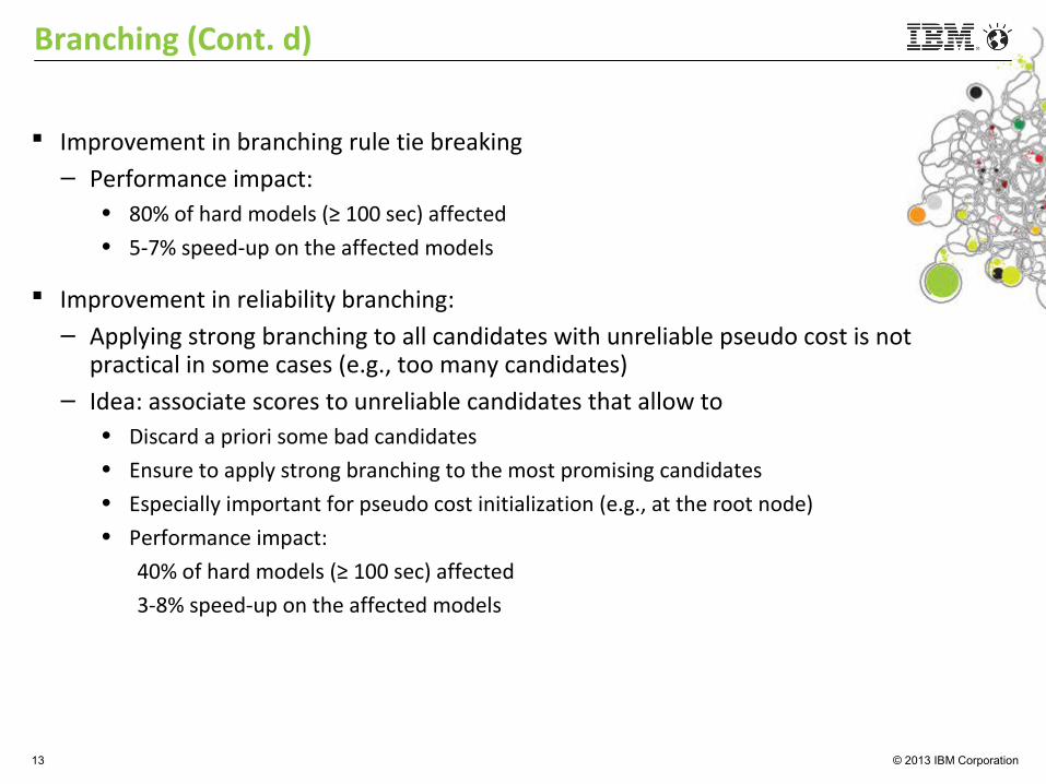
Improvement in branching rule tie breaking– Performance impact:

• 80% of hard models (≥ 100 sec) affected• 5-7% speed-up on the affected models

Improvement in reliability branching:– Applying strong branching to all candidates with unreliable pseudo cost is not

practical in some cases (e.g., too many candidates)– Idea: associate scores to unreliable candidates that allow to

• Discard a priori some bad candidates• Ensure to apply strong branching to the most promising candidates• Especially important for pseudo cost initialization (e.g., at the root node)• Performance impact:

40% of hard models (≥ 100 sec) affected

3-8% speed-up on the affected models

13

Branching (Cont. d)





14

Outline


Implications:– Relationships between binary variables and non-binary variables:

z = 1 --> y ≤ D, with z in {0, 1}, L ≤ y ≤ U, D < U

– Discovered during presolve and probing– Or explicitly given as indicator constraints

Implied bound cuts:

y ≤ U + (D-U) z

Obvious claim: If U1 < U2, then

y ≤ U1 + (D-U1) z dominates y ≤ U2 + (D-U2) z

15

Local implied bound cuts: implications and cutting planes


Global implied bound cuts:– Globally valid implications– Globally valid bounds L, U on implied non-binary variables– Separated at the root node and at branch-and-bound nodes

Local implied bound cuts (new in CPLEX 12.6.1)– Globally valid implications– Locally valid bounds L, U on implied non-binary variables– Separated at branch-and-bound nodes only

New parameter to control local implied bound cuts:– -1 = disabled– 0 = automatic (let CPLEX choose, currently equivalent to -1)– 1 = moderate: separated at starts of new dives, under conservative restrictions– 2 = aggressive: separated at starts of new dives, more often– 3 = very aggressive: potentially separated at every node

Globally valid implications

16

Local implied bound cuts: global cuts versus local cuts


Enabling moderate separation of local implied bound cuts:– 1-2% degradation (neutral?) on our test bed

Key points to be investigated:– Cut strength versus cut validity

• Local cuts are stronger, but global cuts applies to the whole tree

– Interaction with other cut types– Cut filtering and cut selection

• Local cuts are violated more often than global cuts: special filtering rules?

Disabled by default, but fundamental in some cases (e.g., to handle “bigM constraints”)

17

Local implied bound cuts: estimated performance impact


MIQP models arising from a classification problem (Brooks, 2011):

Key point: – Implications are the core of the problem– Very large bounds on α and ωj make any global cut completely ineffective.

min 0.5 ωTQ ω + cT y + 2cT z s.t. zi = 0 --> Ki (ω

T ai + α) + yi ≥ 1, i = 1, …, n zi in {0, 1}, i = 1, …, n 0 ≤ yi ≤ 2, i = 1, …, n

-M ≤ ωj ≤ M, j = 1, …, d -M ≤ α ≤ M.

with M = 108

18

Local implied bound cuts: a case study


Indicator constraints

are translated to

where Li is inferred from global bounds on α and ωj

Bounds Li are just too big and global implied bound cuts

are totally ineffective

Local implied bound cuts:–Two levels of branching immediately yield reasonable local bounds on α and ωj

variables–Local bounds Li on si variables become tight

–Local implied bound cuts are effective

19

Local implied bound cuts: a case study (Cont. d)

zi = 0 --> Ki (ωT ai + α) + yi ≥ 1

Ki (ωT ai + α) + yi - si ≥ 1,

si ≥ -Li, zi = 0 --> si ≥ 0

si ≥ - Li zi


Benchmarks on 30 models (time limit = 10k sec)

– Solver A: CPLEX 12.6.1 default• 22 timeouts• 134.2 sec (geomean) on the 8 solved models

– Solver B: CPLEX 12.6.1 with local implied bound cuts set to very aggressive• 7 timeouts• 469.8 sec (geomean) on the 23 solved models• 23.2 sec (geomean) on the 8 models also solved by default • Speed-up:

4.8x on the 23 solved models by solver B

5.8x on the 8 models solved by both solvers

20

Local implied bound cuts: a case study (Cont. d, 2)





21

Outline


CPLEX Python API and support for Python 3

– Details in: Ryan Kersh, Wednesday 14:45 – 16:15: "Best Practices using the CPLEX Python API”

New parameter to control product linearization in MIQP

– Linearization of products of variables can have a large performance impact• E.g., MIQP can be easily transformed to a MILP if the quadratic objective function contains

binary variables only

– By default, CPLEX will adopt the strategy that looks more promising

– The new parameter QToLin allows the user to explicitly disable or enable the linearization

22

CPLEX 12.6.1 features


Distributed Parallel MIP – Similar to Yuji Shinano et al. (ParaSCIP and ParaCPLEX)– One master process coordinates k workers– Racing ramp-up phase

• all workers solve model, each with different parameter configuration• regular synchronization to report status and share primal and dual bounds• automatic stop criterion selects winner

– Distributed parallel branch-and-cut phase• Nodes of the tree created by the winner are distributed to workers• Workers process nodes they receive as supernodes: presolve, cutting planes, etc.• Rebalancing at sync points

Distributed Concurrent MIP – Infinite horizon ramp-up– This is the option active by default

Both algorithms – already available in CPLEX 12.6.0, deterministic only– can now be deterministic or opportunistic

23

New! Specify settings in VMC file for ramp-up

only

New!

Distributed Memory MIP


1.00

0.86

1.25

1.07

1.00

0.84 0.

96

0.78

1.00

0.87

0.76

0.61

1.00

0.97

0.69

0.56

0

0.2

0.4

0.6

0.8

1

1.2

1.4

>1s >10s >100s >1000s

Default

Opportunistic

DistDet4

DistOpp4

24

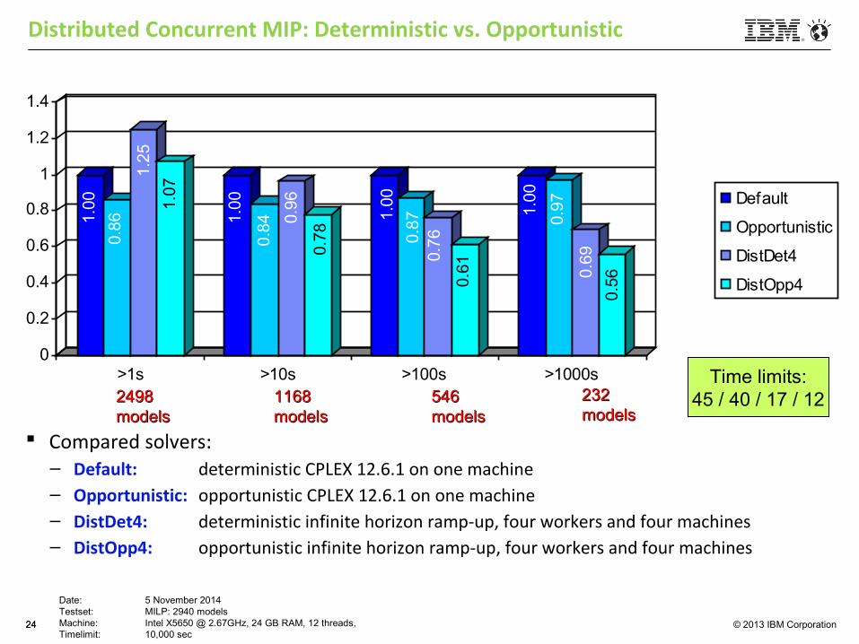
Distributed Concurrent MIP: Deterministic vs. Opportunistic

24



546546modelsmodels

Time limits:45 / 40 / 17 / 12

Date: 5 November 2014Testset: MILP: 2940 modelsMachine: Intel X5650 @ 2.67GHz, 24 GB RAM, 12 threads, Timelimit: 10,000 sec

232232modelsmodels

Compared solvers:– Default: deterministic CPLEX 12.6.1 on one machine– Opportunistic: opportunistic CPLEX 12.6.1 on one machine– DistDet4: deterministic infinite horizon ramp-up, four workers and four machines– DistOpp4: opportunistic infinite horizon ramp-up, four workers and four machines

Software

Recent Advances in CPLEX 12.6.1