Scalable Software Testing and Verification of Non-Functional Properties through Heuristic Search and Optimization

Scalable Software Testing and Verification of Non-Functional Properties through

Heuristic Search and Optimization

Lionel Briand

Interdisciplinary Centre for ICT Security, Reliability, and Trust (SnT)University of Luxembourg, Luxembourg

ITEQS, March 13, 2017

Collaborative Research @ SnT Centre

• Research in context• Addresses actual needs• Well-defined problem• Long-term collaborations• Our lab is the industry

2

Scalable Software Testing and Verification Through Heuristic

Search and Optimization

3

With a focus on non-functional properties

Verification, Testing

• The term “verification” is used in its wider sense: Defect detection.

• Testing is, in practice, the most common verification technique.

• Other forms of verifications are important too (e.g., design time, run-time), but much less present in practice.

4

Decades of V&V research have not yet significantly and widely impacted engineering practice

5

Cyber-Physical Systems

• Increasingly complex and critical systems

• Complex environment • Combinatorial and state

explosion• Dynamic behavior• Complex requirements, e.g.,

temporal, timing, resource usage

• Uncertainty, e.g., about the environment

6

Scalable? Practical?

• Scalable: Can a technique be applied on large artifacts (e.g., models, data sets, input spaces) and still provide useful support within reasonable effort, CPU and memory resources?

• Practical: Can a technique be efficiently and effectively applied by engineers in realistic conditions? – realistic ≠ universal– feasibility and cost of inputs to be provided?

7

Metaheuristics

• Heuristic search (Metaheuristics): Hill climbing, Tabusearch, Simulated Annealing, Genetic algorithms, Ant colony optimisation ….

• Stochastic optimization: General class of algorithms and techniques which employ some degree of randomness to find optimal (or as optimal as possible) solutions to hard problems

• Many verification and testing problems can be re-expressed as optimization problems

• Goal: Address scalability and practicality issues

8

Talk Outline

• Selected project examples, with industry collaborations

• Similarities and patterns

• Lessons learned

9

Testing Software Controllers

References:

10

• R. Matinnejad et al., “Automated Test Suite Generation for Time-continuous Simulink Models“, IEEE/ACM ICSE 2016

• R. Matinnejad et al., “Effective Test Suites for Mixed Discrete-Continuous StateflowControllers”, ACM ESEC/FSE 2015 (Distinguished paper award)

• R. Matinnejad et al., “MiL Testing of Highly Configurable Continuous Controllers: Scalable Search Using Surrogate Models”, IEEE/ACM ASE 2014 (Distinguished paper award)

• R. Matinnejad et al., “Search-Based Automated Testing of Continuous Controllers: Framework, Tool Support, and Case Studies”, Information and Software Technology, Elsevier (2014)

Electronic Control Units (ECUs)

More functions

Comfort and variety

Safety and reliability

Faster time-to-market

Less fuel consumption

Greenhouse gas emission laws

11

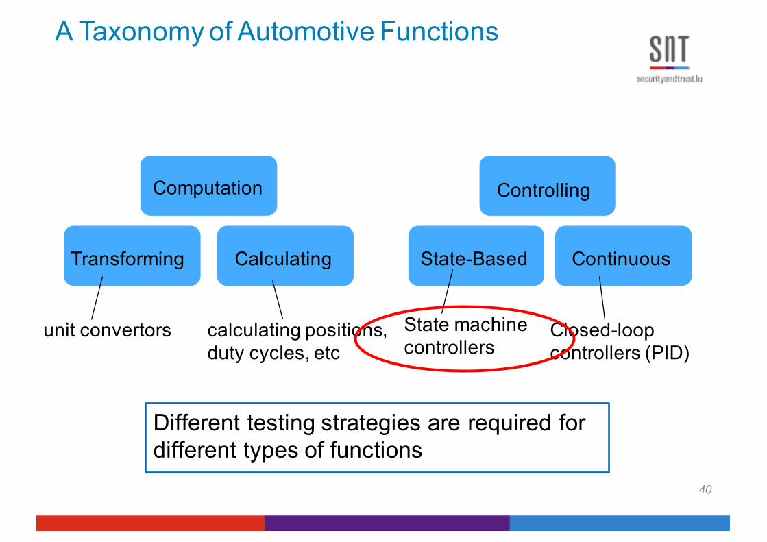
A Taxonomy of Automotive Functions

ControllingComputation

State-Based ContinuousTransforming Calculating

unit convertors calculating positions, duty cycles, etc

State machinecontrollers

Closed-loopcontrollers (PID)

12

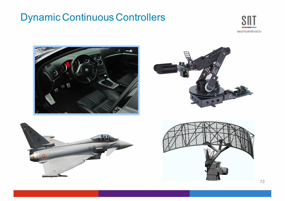
Dynamic Continuous Controllers

13

Development Process

14

Hardware-in-the-Loop Stage

Model-in-the-Loop Stage

Simulink Modeling

Generic Functional

Model

MiL Testing

Software-in-the-Loop Stage

Code Generationand Integration

Software Running on ECU

SiL Testing

SoftwareRelease

HiL Testing

MATLAB/Simulink model

++

0.051FuelLevelSensor

-0.05

1000.8

+-

Gain

Gain1

Add1

Add

1FuelLevel

ContinuousIntegrator

15

• Data flow oriented• Blocks and lines• Time continuous and discrete behavior• Input and outputs signals

Automotive Example

• Supercharger bypass flap controller• Flap position is bounded within [0..1]• 34 sub-components decomposed into 6

abstraction levels• Compressor blowing to the engine

Supercharger

Bypass Flap

Supercharger

Bypass Flap

Flap position = 0 (open) Flap position = 1 (closed)16

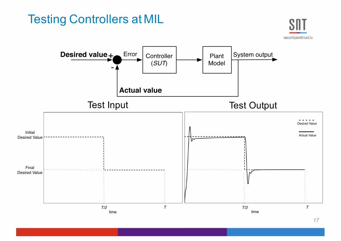
Testing Controllers at MIL

InitialDesired Value

FinalDesired Value

time time

Desired Value

Actual Value

T/2 T T/2 T

Test Input Test Output

Plant Model

Controller(SUT)

Desired value Error

Actual value

System output+-

17

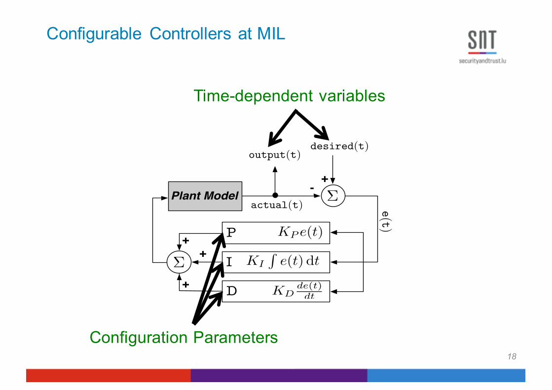
Configurable Controllers at MIL

18

Plant Model

++

+

⌃

+-

e(t)

actual(t)

desired(t)

⌃

KP e(t)

KDde(t)dt

KI

Re(t) dt

P

I

D

output(t)

Time-dependent variables

Configuration Parameters

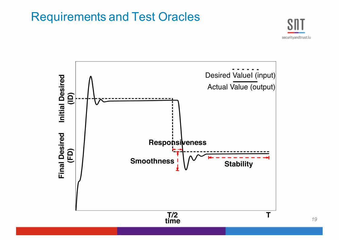
Requirements and Test Oracles

19

Initi

al D

esire

d(ID

)Desired ValueI (input)Actual Value (output)

Fina

l Des

ired

(FD

)

timeT/2 T

Smoothness

Responsiveness

Stability

Test Strategy: A Search-Based Approach

20

Initial Desired (ID)

Fina

l Des

ired

(FD

)

Worst Case(s)?

• Continuous behavior• Controller’s behavior can

be complex• Meta-heuristic search in

(large) input space: Finding worst case inputs

• Possible because of automated oracle (feedback loop)

• Different worst cases for different requirements

• Worst cases may or may not violate requirements

Search-Based Software Testing

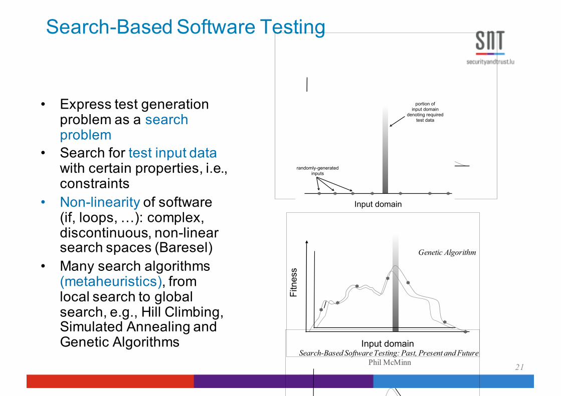
• Express test generation problem as a search problem

• Search for test input data with certain properties, i.e., constraints

• Non-linearity of software (if, loops, …): complex, discontinuous, non-linear search spaces (Baresel)

• Many search algorithms (metaheuristics), from local search to global search, e.g., Hill Climbing, Simulated Annealing and Genetic Algorithms

Section IV discusses future directions for Search-BasedSoftware Testing, comprising issues involving executionenvironments, testability, automated oracles, reduction ofhuman oracle cost and multi-objective optimisation. Finally,Section V concludes with closing remarks.

II. SEARCH-BASED OPTIMIZATION ALGORITHMS

The simplest form of an optimization algorithm, andthe easiest to implement, is random search. In test datageneration, inputs are generated at random until the goal ofthe test (for example, the coverage of a particular programstatement or branch) is fulfilled. Random search is very poorat finding solutions when those solutions occupy a very smallpart of the overall search space. Such a situation is depictedin Figure 2, where the number of inputs covering a particularstructural target are very few in number compared to thesize of the input domain. Test data may be found fasterand more reliably if the search is given some guidance.For meta-heurstic searches, this guidance can be providedin the form of a problem-specific fitness function, whichscores different points in the search space with respect totheir ‘goodness’ or their suitability for solving the problemat hand. An example fitness function is plotted in Figure3, showing how - in general - inputs closer to the requiredtest data that execute the structure of interest are rewardedwith higher fitness values than those that are further away.A plot of a fitness function such as this is referred to as thefitness landscape. Such fitness information can be utilized byoptimization algorithms, such as a simple algorithm calledHill Climbing. Hill Climbing starts at a random point in thesearch space. Points in the search space neighbouring thecurrent point are evaluated for fitness. If a better candidatesolution is found, Hill Climbing moves to that new point,and evaluates the neighbourhood of that candidate solution.This step is repeated, until the neighbourhood of the currentpoint in the search space offers no better candidate solutions;a so-called ‘local optima’. If the local optimum is not theglobal optimum (as in Figure 3a), the search may benefitfrom being ‘restarted’ and performing a climb from a newinitial position in the landscape (Figure 3b).

An alternative to simple Hill Climbing is SimulatedAnnealing [22]. Search by Simulated Annealing is similar toHill Climbing, except movement around the search space isless restricted. Moves may be made to points of lower fitnessin the search space, with the aim of escaping local optima.This is dictated by a probability value that is dependenton a parameter called the ‘temperature’, which decreasesin value as the search progresses (Figure 4). The lowerthe temperature, the less likely the chances of moving to apoorer position in the search space, until ‘freezing point’ isreached, from which point the algorithm behaves identicallyto Hill Climbing. Simulated Annealing is named so becauseit was inspired by the physical process of annealing inmaterials.

Input domain

portion of input domain

denoting required test data

randomly-generatedinputs

Figure 2. Random search may fail to fulfil low-probability test goals

Fitn

ess

Input domain

(a) Climbing to a local optimum

Fitn

ess

Input domain(b) Restarting, on this occasion resulting in a climb to the global optimum

Figure 3. The provision of fitness information to guide the search withHill Climbing. From a random starting point, the algorithm follows thecurve of the fitness landscape until a local optimum is found. The finalposition may not represent the global optimum (part (a)), and restarts maybe required (part (b))

Fitn

ess

Input domainFigure 4. Simulated Annealing may temporarily move to points of poorerfitness in the search space

Fitn

ess

Input domainFigure 5. Genetic Algorithms are global searches, sampling many pointsin the fitness landscape at once

Search-Based Software Testing: Past, Present and Future Phil McMinn

Genetic Algorithm

21

Section IV discusses future directions for Search-BasedSoftware Testing, comprising issues involving executionenvironments, testability, automated oracles, reduction ofhuman oracle cost and multi-objective optimisation. Finally,Section V concludes with closing remarks.

II. SEARCH-BASED OPTIMIZATION ALGORITHMS

The simplest form of an optimization algorithm, andthe easiest to implement, is random search. In test datageneration, inputs are generated at random until the goal ofthe test (for example, the coverage of a particular programstatement or branch) is fulfilled. Random search is very poorat finding solutions when those solutions occupy a very smallpart of the overall search space. Such a situation is depictedin Figure 2, where the number of inputs covering a particularstructural target are very few in number compared to thesize of the input domain. Test data may be found fasterand more reliably if the search is given some guidance.For meta-heurstic searches, this guidance can be providedin the form of a problem-specific fitness function, whichscores different points in the search space with respect totheir ‘goodness’ or their suitability for solving the problemat hand. An example fitness function is plotted in Figure3, showing how - in general - inputs closer to the requiredtest data that execute the structure of interest are rewardedwith higher fitness values than those that are further away.A plot of a fitness function such as this is referred to as thefitness landscape. Such fitness information can be utilized byoptimization algorithms, such as a simple algorithm calledHill Climbing. Hill Climbing starts at a random point in thesearch space. Points in the search space neighbouring thecurrent point are evaluated for fitness. If a better candidatesolution is found, Hill Climbing moves to that new point,and evaluates the neighbourhood of that candidate solution.This step is repeated, until the neighbourhood of the currentpoint in the search space offers no better candidate solutions;a so-called ‘local optima’. If the local optimum is not theglobal optimum (as in Figure 3a), the search may benefitfrom being ‘restarted’ and performing a climb from a newinitial position in the landscape (Figure 3b).

An alternative to simple Hill Climbing is SimulatedAnnealing [22]. Search by Simulated Annealing is similar toHill Climbing, except movement around the search space isless restricted. Moves may be made to points of lower fitnessin the search space, with the aim of escaping local optima.This is dictated by a probability value that is dependenton a parameter called the ‘temperature’, which decreasesin value as the search progresses (Figure 4). The lowerthe temperature, the less likely the chances of moving to apoorer position in the search space, until ‘freezing point’ isreached, from which point the algorithm behaves identicallyto Hill Climbing. Simulated Annealing is named so becauseit was inspired by the physical process of annealing inmaterials.

Input domain

portion of input domain

denoting required test data

randomly-generatedinputs

Figure 2. Random search may fail to fulfil low-probability test goals

Fitn

ess

Input domain

(a) Climbing to a local optimum

Fitn

ess

Input domain(b) Restarting, on this occasion resulting in a climb to the global optimum

Figure 3. The provision of fitness information to guide the search withHill Climbing. From a random starting point, the algorithm follows thecurve of the fitness landscape until a local optimum is found. The finalposition may not represent the global optimum (part (a)), and restarts maybe required (part (b))

Fitn

ess

Input domainFigure 4. Simulated Annealing may temporarily move to points of poorerfitness in the search space

Fitn

ess

Input domainFigure 5. Genetic Algorithms are global searches, sampling many pointsin the fitness landscape at once

22

Search Elements

• Search Space:• Initial and desired values, configuration parameters

• Search Technique:• (1+1) EA, variants of hill climbing, GAs …

• Search Objective: • Objective/fitness function for each requirement

• Evaluation of Solutions• Simulation of Simulink model => fitness computation

• Result: • Worst case scenarios or input signals that (are more likely to) break the requirement at MiL level

22

Smoothness Objective Functions: OSmoothness

Test Case A Test Case B

OSmoothness(Test Case A) > OSmoothness(Test Case B)

We want to find test scenarios which maximize OSmoothness

23

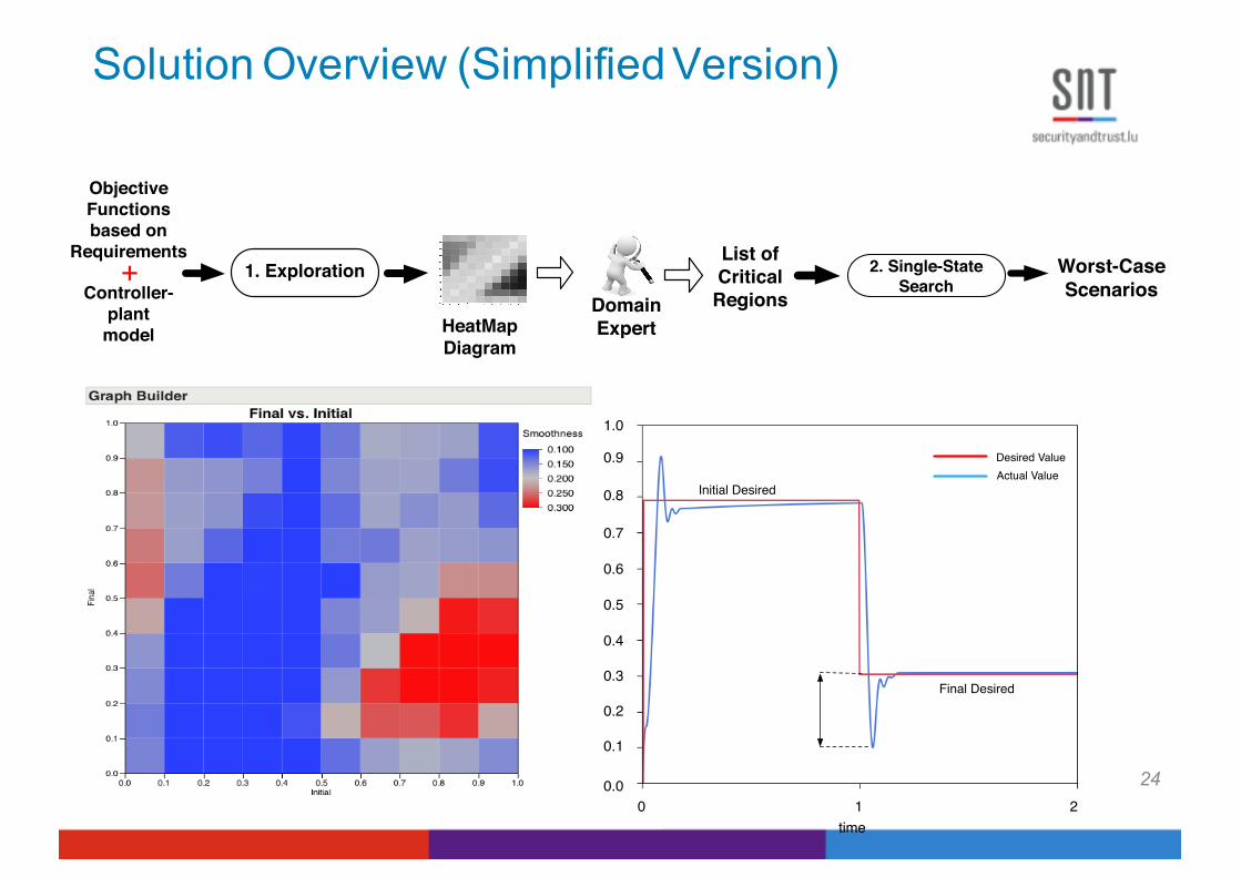
Solution Overview (Simplified Version)

24

HeatMap Diagram

1. ExplorationList of Critical RegionsDomain

Expert

Worst-Case Scenarios

+Controller-

plant model

Objective Functionsbased on

Requirements 2. Single-State

Search

time

Desired ValueActual Value

0 1 20.0

0.1

0.2

0.3

0.4

0.5

0.6

0.7

0.8

0.9

1.0

Initial Desired

Final Desired

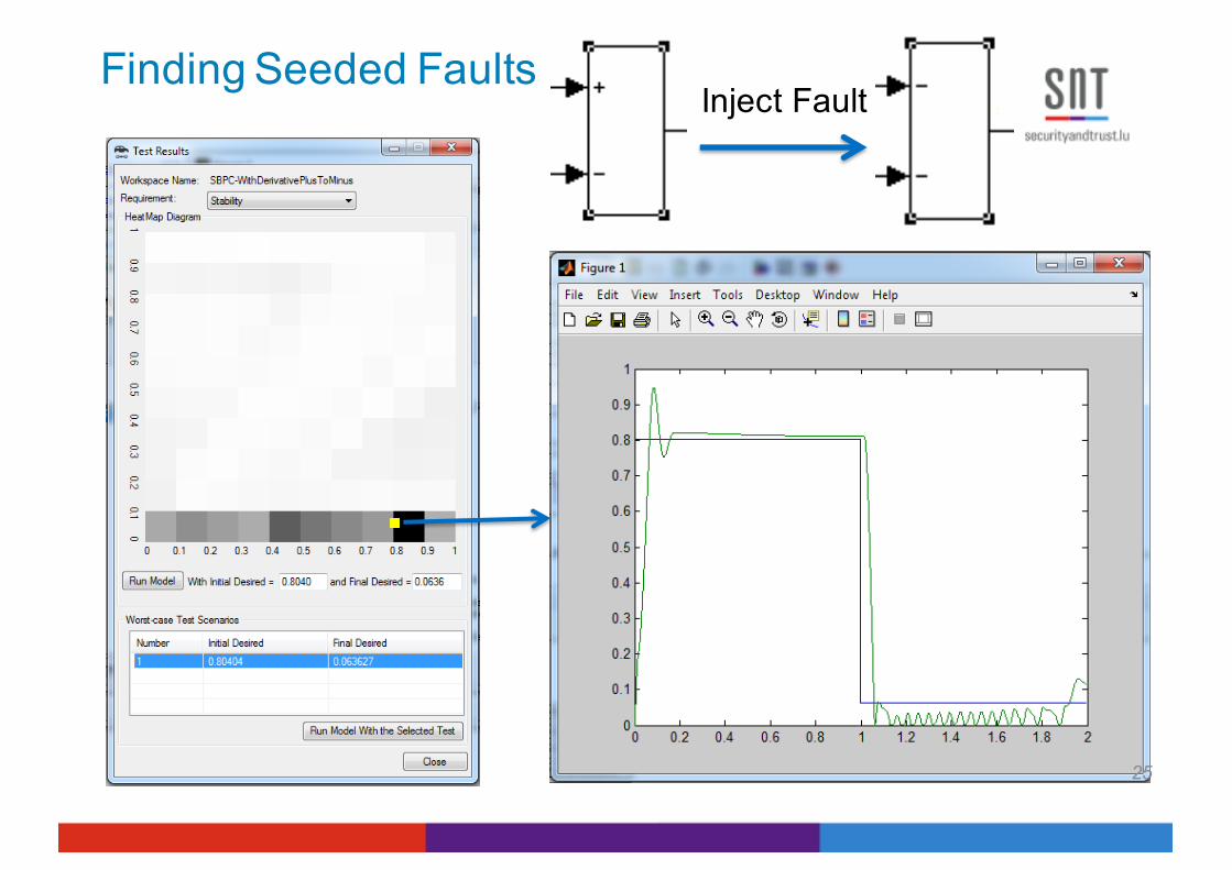
Finding Seeded FaultsInject Fault

25

Analysis – Fitness increase over iterations

26Number of Iterations

Fitn

ess

Analysis II – Search over different regions

27

0.315

0.316

0.317

0.319

0.321

0.323

0.324

0.326

0.327

0.329

0.330

0 10 20 30 40 50 60 70 80 90 100

0.328

0.325

0.320

0.318

0 10 20 30 40 50 60 70 80 90 1000 10 20 30 40 50 60 70 80 90 100

Random Search(1+1) EA

0 10 20 30 40 50 60 70 80 90 100

0.0166

0.0168

0.0170

0.0176

0.0180

0.0178

0.0172

0.0160

0.0162

0.0164 Random Search(1+1) EA

0 10 20 30 40 50 60 70 80 90 100 0 10 20 30 40 50 60 70 80 90 100

0.0174

Average (1+1) EA Distribution Random Search Distribution

Number of Iterations

• We found much worse scenarios during MiL testing than our partner had found so far, and much worse than random search (baseline)

• These scenarios are also run at the HiL level, where testing is much more expensive: MiL results -> test selection for HiL

• But further research was needed:– Simulations are expensive – Configuration parameters – Dynamically adjust search algorithms in different

subregions (exploratory <-> exploitative)

Conclusions

i.e., 31s. Hence, the horizontal axis of the diagrams in Figure 8 shows the number ofiterations instead of the computation time. In addition, we start both random search and(1+1) EA from the same initial point, i.e., the worst case from the exploration step.

Overall in all the regions, (1+1) EA eventually reaches its plateau at a value higherthan the random search plateau value. Further, (1+1) EA is more deterministic than ran-dom, i.e., the distribution of (1+1) EA has a smaller variance than that of random search,especially when reaching the plateau (see Figure 8). In some regions (e.g., Figure 8(d)),however, random reaches its plateau slightly faster than (1+1) EA, while in some otherregions (e.g. Figure 8(a)), (1+1) EA is faster. We will discuss the relationship betweenthe region landscape and the performance of (1+1) EA in RQ3.RQ3. We drew the landscape for the 11 regions in our experiment. For example, Fig-ure 9 shows the landscape for two selected regions in Figures 7(a) and 7(b). Specifically,Figure 9(a) shows the landscape for the region in Figure 7(b) where (1+1) EA is fasterthan random, and Figure 9(b) shows the landscape for the region in Figure 7(a) where(1+1) EA is slower than random search.

0.30

0.31

0.32

0.33

0.34

0.35

0.36

0.37

0.38

0.39

0.40

0.70 0.71 0.72 0.73 0.74 0.75 0.76 0.77 0.78 0.79 0.800.10

0.11

0.12

0.13

0.14

0.15

0.16

0.17

0.18

0.19

0.20

0.90 0.91 0.92 0.93 0.94 0.95 0.96 0.97 0.98 0.99 1.00

(a) (b)

Fig. 9. Diagrams representing the landscape for two representative HeatMap regions: (a) Land-scape for the region in Figure 7(b). (b) Landscape for the region in Figure 7(a).

Our observations show that the regions surrounded mostly by dark shaded regionstypically have a clear gradient between the initial point of the search and the worst casepoint (see e.g., Figure 9(a)). However, dark regions located in a generally light shadedarea have a noisier shape with several local optimum (see e.g., Figure 9(b)). It is knownthat for regions like Figure 9(a), exploitative search works best, while for those like Fig-ure 9(b), explorative search is most suitable [10]. This is confirmed in our work wherefor Figure 9(a), our exploitative search, i.e., (1+1) EA with � = 0.01, is faster and moreeffective than random search, whereas for Figure 9(b), our search is slower than randomsearch. We applied a more explorative version of (1+1) EA where we let � = 0.03 to theregion in Figure 9(b). The result (Figure 10) shows that the more explorative (1+1) EAis now both faster and more effective than random search. We conjecture that, from theHeatMap diagrams, we can predict which search algorithm to use for the single-statesearch step. Specifically, for dark regions surrounded by dark shaded areas, we suggestan exploitative (1+1) EA (e.g., � = 0.01), while for dark regions located in light shadedareas, we recommend a more explorative (1+1) EA (e.g., � = 0.03).

6 Related WorkTesting continuous control systems presents a number of challenges, and is not yet sup-ported by existing tools and techniques [4, 1, 3]. The modeling languages that have been

13

28

Testing in the Configuration Space

• MIL testing for all feasible configurations

• The search space is much larger

• The search is much slower (Simulations of Simulink models are expensive)

• Results are harder to visualize

• But not all configuration parameters matter for all objective functions

29

Modified Process and Technology

30

+Controller

Model (Simulink)

Worst-Case Scenarios

List of Critical

PartitionsRegressionTree

1.Exploration with Dimensionality

Reduction

2.Search withSurrogate Modeling

Objective Functions

DomainExpert

Visualization of the 8-dimension space using regression treesDimensionality

reduction to identify the significant variables(Elementary Effect Analysis)

Surrogate modeling to predict the objective function and speed up the search (Machine learning)

Dimensionality Reduction

• Sensitivity Analysis: Elementary Effect Analysis (EEA)

• Identify non-influential inputs in computationally costly mathematical models

• Requires less data points than other techniques

• Observations are simulations generated during the Exploration step

• Compute sample mean and standard deviation for each dimension of the distribution of elementary effects

31

Cal5ID

Cal3FD

Cal4Cal6

Cal1,Cal2

0.6

0.4

0.2

0.0

Sam

ple

Stan

dard

Dev

iatio

n (

)

-0.6 -0.4 -0.2 0.0 0.2Sample Mean ( )

⇤10�2

⇤10�2

S� i

�i

Elementary Effects Analysis Method

ü Imagine function F with 2 inputs, x and y:

A �x

�y

A1

A2

C �x

�y

C1

C2

B �x

�y

B1

B2

X

Y

Elementary Effectsfor X for Y

F(A1)-F(A)F(B1)-F(B)F(C1)-F(C)

…

F(A2)-F(A)F(B2)-F(B)F(C2)-F(C)

…

32

Visualization in Inputs & Configuration Space

33

All Points

FD>=0.43306

Count MeanStd Dev

Count MeanStd Dev

FD<0.43306Count MeanStd Dev

ID>=0.64679Count MeanStd Dev

Count MeanStd Dev

Cal5>=0.020847 Cal5>0.020847Count MeanStd Dev

Count MeanStd Dev

Cal5>=0.014827 Cal5<0.014827Count MeanStd Dev

Count MeanStd Dev

1000 0.007822

0.0049497

ID<0.64679

574 0.00595130.0040003

426 0.01034250.0049919

373 0.00475940.0034346

201 0.00816310.0040422

182 0.01345550.0052883

244 0.00802060.0031751

70 0.01067950.0052045

131 0.00681850.0023515 Regression Tree

Surrogate Modeling During Search

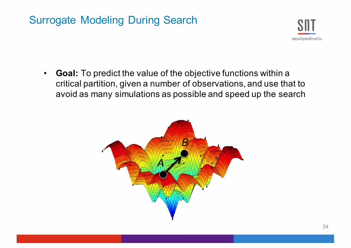
• Goal: To predict the value of the objective functions within a critical partition, given a number of observations, and use that to avoid as many simulations as possible and speed up the search

34

A

B

Surrogate Modeling During Search

35

• Any supervised learning or statistical technique providing fitness predictions with confidence intervals

1. Predict higher fitness with high confidence: Move to new position, no simulation

2. Predict lower fitness with high confidence: Do not move to new position, no simulation

3. Low confidence in prediction: Simulation

Surrogate Model

Real Function

x

Fitness

Experiments Results (RQ1)

ü The best regression technique to build Surrogate models for all of our three objective functions is Polynomial Regression with n = 3ü Other supervised learning techniques, such as SVM

Mean of R2/MRPE values for different surrogate modeling techniques

Fst

Fsm

Fr

PR(n=3)R2/MRPE

0.66/0.0526 0.95/0.0203

0.78/0.0295

0.26/0.2043

0.98/0.0129

0.85/0.0247 0.85/0.0245

0.46/0.1755 0.54/0.1671

0.44/0.0791

0.49/1.2281

0.22/1.2519

LRR2/MRPE

ERR2/MRPE

PR(n=2)R2/MRPE

36


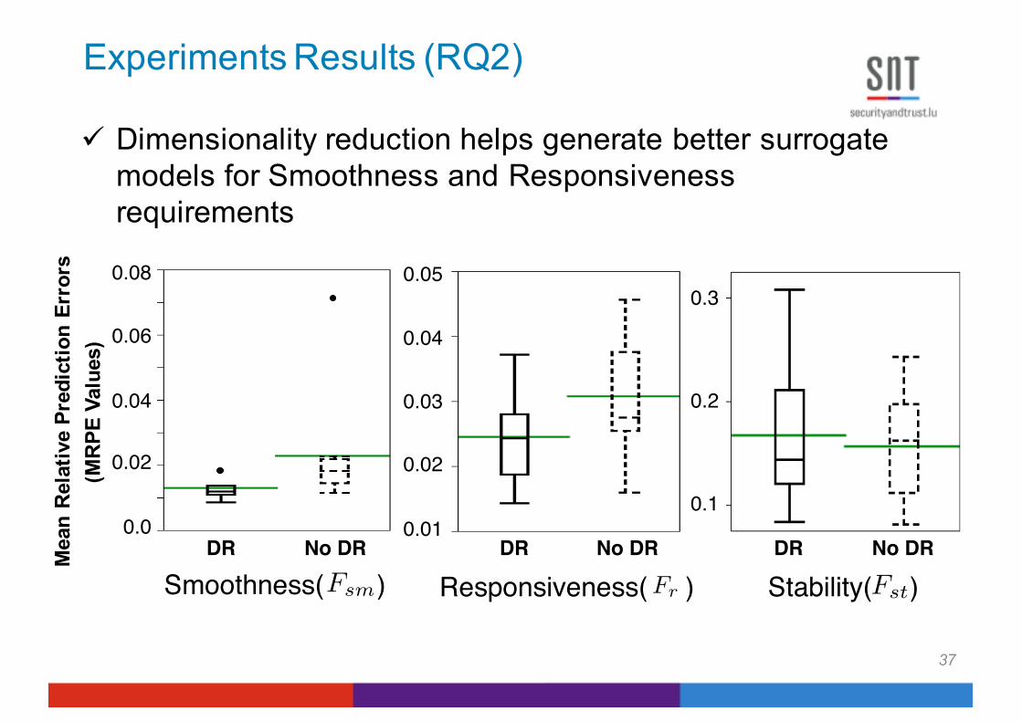
ü Dimensionality reduction helps generate better surrogate models for Smoothness and Responsiveness requirements

0.0

0.02

0.04

0.06

0.08 0.05

0.01

0.02

0.03

0.04

0.1

0.2

0.3

DR No DR DR No DR DR No DR

Smoothness( )Fsm Responsiveness( )Fr Stability( )Fst

Mea

n Re

lativ

e Pr

edic

tion

Erro

rs

(MRP

E Va

lues

)

37

ü For responsiveness, the search with SM was 8 times faster

ü For smoothness, the search with SM was much more effective


Sear

ch O

utpu

tVa

lues

Sear

ch O

utpu

tVa

lues

0.215SM

After 800 seconds After 2500 seconds After 3000 seconds

NoSM

0.220

0.225

0.230

0.235

SM NoSMSM NoSM

After 200 seconds

0.160

0.164

0.168

After 300 seconds After 3000 seconds

NoSM NoSM SM NoSMSM SM

38

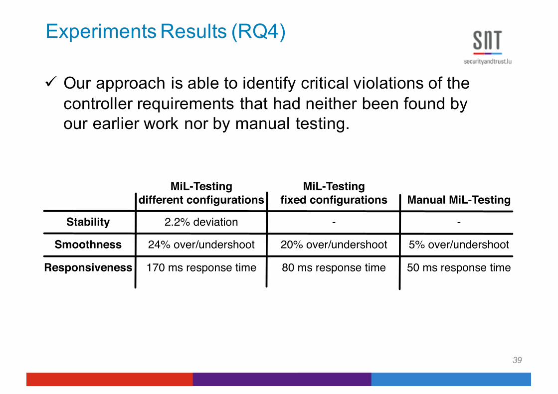
ü Our approach is able to identify critical violations of the controller requirements that had neither been found by our earlier work nor by manual testing.

MiL-Testing different configurations

Stability

Smoothness

Responsiveness

MiL-Testing fixed configurations Manual MiL-Testing

- -2.2% deviation

24% over/undershoot 20% over/undershoot 5% over/undershoot

170 ms response time 80 ms response time 50 ms response time


39

A Taxonomy of Automotive Functions

ControllingComputation

State-Based ContinuousTransforming Calculating

unit convertors calculating positions, duty cycles, etc

State machinecontrollers

Closed-loopcontrollers (PID)

Different testing strategies are required for different types of functions

40

Open-Loop Controllers

41

respectively. In addition, we adapt the whitebox coverage and theblackbox output diversity selection criteria to Stateflows, and evalu-ate their fault revealing power for continuous behaviours. Coveragecriteria are prevalent in software testing and have been consideredin many studies related to test suite effectiveness in different appli-cation domains [?]. In our work, we consider state and transitioncoverage criteria [?] for Statflows. Our output diversity criterion isbased on the recent output uniqueness criterion [?] that has beenstudied for web applications and has shown to be a useful surro-gate to whitebox selection techniques. We consider this criterionin our work because Stateflows have complex internal structuresconsisting of differential equations, making them less amenable towhitebox techniques, while they have rich time-continuous outputs.

In this paper, we make the following contributions:

• We focus on the problem of testing Stateflows with mixeddiscrete-continuous behaviours. We propose two new testcase selection criteria output stability and output continuitywith the goal of selecting test inputs that are likely to pro-duce continuous outputs exhibiting instability and disconti-nuity failures, respectively.

• We adapt the whitebox coverage and the blackbox outputdiversity selection criteria to Stateflows, and evaluate theirfault revealing power for continuous behaviours. The formeris defined based on traditional state and transition coveragefor state machines, and the latter is defined based on the re-cent output uniqueness criterion [?].

• We evaluate effectiveness of our newly proposed and theadapted selection criteria by applying them to three Stateflowcase study models: two industrial and one public domain.Our results show that RESULT.

Organization of the paper.

2. BACKGROUND AND MOTIVATIONMotivating example. We motivate our work using a simplifiedStateflow from the automotive domain which controls a superchargerclutch and is referred to as the Supercharger Clutch Controller (SCC).Figure 1(a) represents the discrete behaviour of SCC specifyingthat the supercharger clutch can be in two quiescent states [?]: en-gaged or disengaged. Further, the clutch moves from the disen-gaged to the engaged state whenever both the engine speed engspdand the engine coolant temperature tmp respectively fall inside thespecified ranges of [smin..smax] and [tmin..tmax]. The clutchmoves back from the engaged to the disengaged state whenevereither the speed or the temperature falls outside their respectiveranges. The variable ctrlSig in Figure 1(a) indicates the sign andmagnitude of the voltage applied to the DC motor of the clutchto physically move the clutch between engaged and disengagedpositions. Assigning 1.0 to ctrlSig moves the clutch to the en-gaged position, and assigning �1.0 to ctrlSig moves it back tothe disengaged position. To avoid clutter in our figures, we useengageReq to refer to the condition on the Disengaged ! En-gaged transition, and disengageReq to refer to the condition onthe Engaged ! Disengaged transition.

The discrete transition system in Figure 1(a) assumes that theclutch movement takes no time, and further, does not provide anyinsight on the quality of movement of the clutch. Figure 1(b) ex-tends the discrete transition system in Figure 1(a) by adding a timervariable, i.e., time, to explicate the passage of time in the SCCbehaviour. The new transition system in Figure 1(b) includes two

(a) SCC -- Discrete Behaviour

(b) SCC -- Timed Behaviour

EngagedDisengaged

Engaging

(c) Engaging state of SCC -- mixed discrete-continuous behaviour

Disengaging

Disengaged

Engaged

time + +;

[disengageReq]/time := 0

[time

>5]

[time

>5]

time + +;

[(engspd > smin � engspd < smax) � (tmp > tmin � tmp < tmax)]/ctrlSig := 1

[engageReq]/ time := 0

[¬(engspd > smin � engspd < smax) � ¬(tmp > tmin � tmp < tmax)] /ctrlSig := �1

OnMoving OnSlipping

OnCompleted

time + +;ctrlSig := f(time)

Engaging

time + +;ctrlSig := g(time)

time + +;ctrlSig := 1.0

[¬(vehspd = 0) �time > 2]

[(vehspd = 0) �time > 3]

[time > 4]

Figure 1: Supercharge Clutch Controller (SCC) Stateflow.

transient states [?], engaging and disengaging, specifying that mov-ing from the engaged to the disengaged state and vice versa takessix milisec. Since this model is simplified, it does not show han-dling of alterations of the clutch state during the transient states.In addition to adding the time variable, we note that the variablectrlSig, which controls physical movement of the clutch, cannotabruptly jump from 1.0 to �1.0, or vice versa. In order to ensuresafe and smooth movement of the clutch, the variable ctrlSig hasto gradually move between 1.0 and �1.0 and be described as afunction over time, i.e., a signal. To express the evolution of thectrlSig signal over time, we decompose the transient states en-gaging and disengaging into sub-state machines. Figure 1(c) showsthe sub-state machine related to the engaging state. The one relatedto the disengaging state is similar. At beginning (in state OnMov-ing), the function ctrlSig has a steep grade (i.e., function f ) tomove the stationary clutch from the disengaged state and acceler-ate it to reach a certain speed in about two milisec. Afterwards (instate OnSlipping), ctrlSig decreases the speed of clutch basedon the gradual function g until about four milisec. This is to ensurethat the clutch slows down as it gets closer to the crank shaft ofthe car. Finally, at state OnCompleted, ctrlSig reaches value 1.0and remains constant, causing the clutch to get engaged in aboutone milisec. When the car is stationary, i.e., vehspd is 0, the clutchmoves based on the steep grade function f for three milisec, anddoes not have to go to the OnSlipping phase to slow down beforeit reaches the crank shaft at state OnCompleted.Input and Output. The Stateflow inputs and outputs are signals(functions over time). Each input/output signal has a data type,e.g. boolean, enum or float, specifying the range of the signal.For example, Figure 2 shows an example input (dashed line) andoutput (solid line) signals for SCC. The input signal is related toengageReq and is boolean, while the output signal is related to

• No feedback loop -> no automated oracle

• No plant model: Much quicker simulation time

• Mixed discrete-continuous behavior: Simulink stateflows

• The main testing cost is the manual analysis of output signals

• Goal: Minimize test suites

• Challenge: Test selection

• Entirely different approach to testing On

Off

CtrlSig

Selection Strategies Based on Search

• Input diversity• White-box Structural

Coverage• State Coverage• Transition Coverage

• Output Diversity• Failure-Based Selection

Criteria • Domain specific failure

patterns• Output Stability• Output Continuity

42

S3t

S3t

Failure-based Test Generation

43

Instability Discontinuity

0.0 1.0 2.0-1.0

-0.5

0.0

0.5

1.0

Time

Ctr

lSig

Output

• Search: Maximizing the likelihood of presence of specific failure patterns in output signals

• Domain-specific failure patterns elicited from engineers

0.0 1.0 2.0Time

0.0

0.25

0.50

0.75

1.0

Ctr

lSig

Output

Summary of Results

• The test cases resulting from state/transition coverage algorithms cover the faulty parts of the models

• However, they fail to generate output signals that are sufficiently distinct from the oracle signal, hence yielding a low fault revealing rate

• Output-based algorithms are more effective

44

Automated Testing of Driver Assistance Systems Through Simulation

Reference:

45

R. Ben Abdessalem et al., "Testing Advanced Driver Assistance Systems Using Multi-Objective Search and Neural Networks”, ACM ESEC/FSE 2016

Pedestrian Detection Vision System (PeVi)

46

• The PeVi system is a camera-basedcollision-warning system providing improved vision

Testing DA Systems

• Testing DA systems requires complex and comprehensive simulation environments– Static objects: roads, weather, etc.– Dynamic objects: cars, humans, animals, etc.

• A simulation environment captures the behavior of dynamic objects as well as constraints and relationships between dynamic and static objects

47

Approach

48

Generation of Test specifications

Static[ranges/values/

resolution]

Dynamic[ranges/

resolution]

(2)

test case specification

Specification Documents(Simulation Environment and PeVi System)

Domain model

Requirements model

(1)Development of Requirementsand domain models

49

- simulationTime: Real- timeStep: Real

Test Scenario

- v0: RealVehicle

- x0: Real

- y0: Real

- θ: Real- v0: Real

Pedestrian

- simulationTime: Real- timeStep: Real

Test Scenario

PeVi

11

11

«positioned» DynamicObject

- v0: RealVehicle

- x0: Real

- y0: Real

- θ: Real- v0: Real

Pedestrian

- x: Real- y: Real

Position

*

11

- state: BooleanCollision

PeVi

- state: BooleanDetection

11

11

- AWA

Output Trajectory

Static inputsDynamic inputsOutputs

- intensity: RealSceneLight

1- weatherType: Condition

Weather

- fog- rain- snow- normal

«enumeration»Condition

- field of view: Real

Camera Sensor

RoadSide Object

- roadType: RTRoad

1 - curved- straight- ramped

«enumeration»RT

1

*

1

Parked Cars

Trees- simulationTime: Real- timeStep: Real

Test Scenario

«uses»1 1 PeVi

PeVi and Environment Domain Model

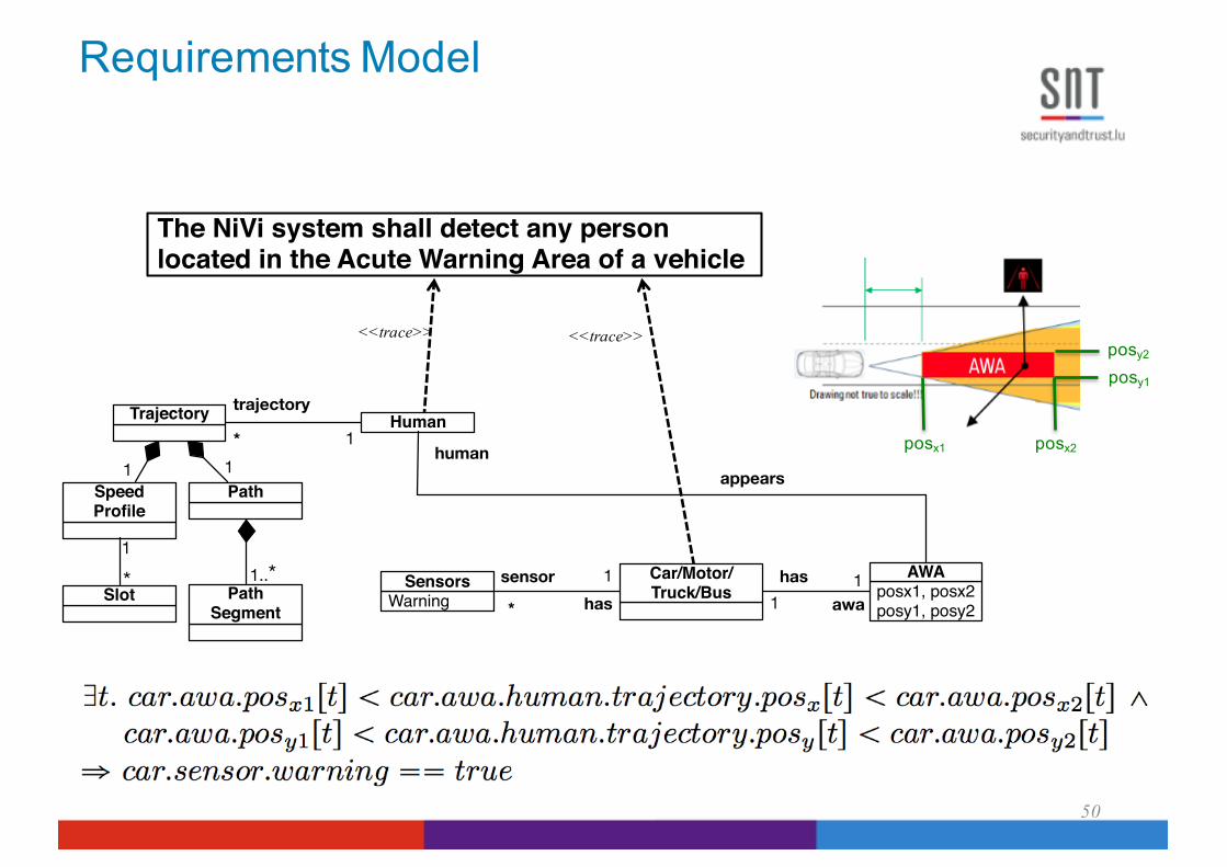
Requirements Model

50

<<trace>> <<trace>>

Speed Profile

Path1 1

Slot Path Segment

1..**1

Trajectory Human1*

trajectory

WarningSensors posx1, posx2

posy1, posy2

AWACar/Motor/Truck/Bus

sensorhas

hasawa

11

1

*

humanappears

posx1 posx2

posy1

posy2

The NiVi system shall detect any person located in the Acute Warning Area of a vehicle

MiL Testing via Search

51

Simulator + NiVi

Environment Settings(Roads, weather, vehicle type, etc.)

Fixed during Search Manipulated by Search

Human Simulator(initial position,

speed, orientation)

Car Simulator(speed)

PeVi

Meta-heuristic Search(multi-objective)

Generate scenarios

Detection or not?

Collision or not?

52

Type of Road Type of vehicle Type of actorSituation 1 Straight Car MaleSituation 2 Straight Car ChildSituation 3 Straight Car CowSituation 4 Straight Truck MaleSituation 5 Straight Truck ChildSituation 6 Straight Truck CowSituation 7 Curved Car MaleSituation 8 Curved Car ChildSituation 9 Curved Car CowSituation 10 Curved Truck MaleSituation 11 Curved Truck ChildSituation 12 Curved Track CowSituation 13 Ramp Car MaleSituation 14 Ramp Car ChildSituation 15 Ramp Car CowSituation 16 Ramp Truck MaleSituation 17 Ramp Truck ChildSituation 18 Ramp Truck CowSituation 19Situation 20

Straight Car+ Cars in parkingCar + buildings

Male

Test Case Specification: Static (combinatorial)

Test Case Specification: Dynamic

53

Start locationX = 74Start locationY = 37.72Start locationZ = 0Orientation = 0

trajectoryPerson : TrajectoryPositionX= 74Position Y= 37.72Position Z = 0OrientationHeading = 93.33Acceleration = 0MaxWalkingSpeed =14height=1.75

person :Actor

UniqueId

profilePerson : Speed Profile

StartPointX = 74StartPointY = 37.72StartPointY = 0StartAngle = 93.33End Angle = 0Length = 60

pathPerson : Path

Length = 60Type = StraightMaxSpeedLimit = 14

segmentPerson : Path Segment

IDslotPerson : Slot

Time = 0Speed = 12.59

startPerson : StartState

Start locationX = 10Start locationY = 50.125Start locationZ = 0.56Orientation = 0

trajectoryCar : TrajectoryPositionX=10Position Y= 50.125Position Z = 0.56OrientationHeading = 0Acceleration = 0MaxWalkingSpeed =100

car : Actor

UniqueId

profileCar : Speed Profile

StartPointX = 10StartPointY = 50.125StartPointZ =0.56StartAngle = 0End Angle = 0Length = 100

pathCar : Path

Length = 100Type = StraightMaxSpeedLimit = 100

segmentCar : Path Segment

IDslotCar : Slot

Time = 0Speed = 60.66

startCar : StartState

MinTTC=0.3191Collision

Choice of Surrogate Model

• Neural networks (NN) have been trained to learn complex functions predicting fitness values

• NN can be trained using different algorithms such as:– LM: Levenberg-Marquardt– BR: Bayesian regularization backpropagation– SCG: Scaled conjugate gradient backpropagation

• R2 (coefficient of determination) indicates how well data fit a statistical model

• Computed R2 for LM, BR and SCG è BR has the highest R2

54

Multi-Objective Search

• Input space: car-speed, person-speed, person-position (x,y), person-orientation

• Search algorithm need objective or fitness functions for guidance

• In our case several independent functions could be interesting:– Minimum distance between car and

pedestrian – Minimum distance between

pedestrian and AWA– Minimum time to collision

• NSGA II algorithm55

posx1 posx2

posy1

posy2

Pareto Front

56

Individual A Pareto dominates individual B ifA is at least as good as B in every objective and better than B in at least one objective.

Dominated by x

O1

O2

Pareto frontx

• A multi-objective optimization algorithm must achieve:• Guide the search towards the global Pareto-Optimal front.• Maintain solution diversity in the Pareto-Optimal front.

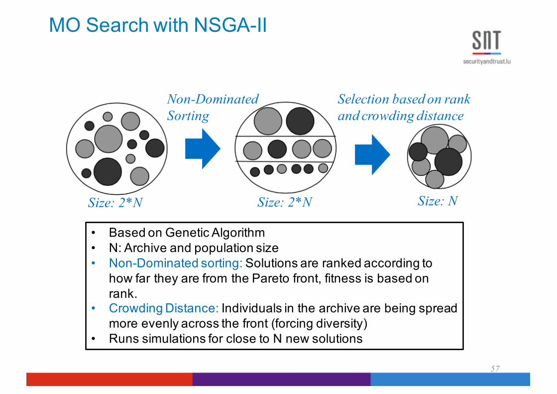
MO Search with NSGA-II

57

Non-Dominated Sorting

Selection based on rank and crowding distance

Size: 2*N Size: 2*N Size: N

• Based on Genetic Algorithm• N: Archive and population size• Non-Dominated sorting: Solutions are ranked according to

how far they are from the Pareto front, fitness is based on rank.

• Crowding Distance: Individuals in the archive are being spread more evenly across the front (forcing diversity)

• Runs simulations for close to N new solutions

Pareto Front Results

58

Pareto Front Projection

59

Simulation Scenario Execution

• Straight road with parking• The person appears in the AWA, but is not detected

60

Improving Time Performance

• Individual simulations take on average more than 1min

• It takes 10 hours to run our search-based test generation (≈ 500 simulations)

• We use surrogate modeling to improve the search • Neural networks are used to predict fitness values

within a confidence interval• During the search, we use prediction values &

confidence intervals to run simulations onlyfor the solutions likely to be selected

61

Search with Surrogate Models

62

Non-Dominated Sorting

Selection based on rank and crowding distance

Size: 2*N Size: 2*N Size: N

Original Algorithm- Runs simulations for allnew solutions

Our Algorithm- Uses prediction values

& intervals to run simulations onlyfor the solutions likely to be selected

NSGA II

Results – Surrogate Modeling

63

0.00

0.25

0.50

0.75

1.00

Time (min)

HV

50 100 15010

(a) Comparing HV values obtained by NSGAII and NSGAII-SM

NSGAII (mean)NSGAII-SM (mean)

0.00

0.25

0.50

0.75

1.00

Time (min)50 100 15010

(b) Comparing HV values obtained by RS and NSGAII-SM

HV

RS (mean)NSGAII-SM (mean)

0.00

0.25

0.50

0.75

1.00

Time (min)

HV

50 100 15010

(c) HV values for worst runs of NSGAII, NSGAII-SM and RS

RS

NSGAII-SM NSGAII

Figure 6: Comparing HV values obtained by (a) 20runs of NSGAII and NSGAII-SM (cl=.95); (b) 20runs of random search and NSGAII-SM (cl=.95);and (c) the worst runs of NSGAII, NSGAII-SM(cl=.95) and random search.

form further experiments by the time of writing of this pa-per. Our current experiment required nine days to complete.In addition, we performed several preliminary and trial anderror experiments to reach optimal algorithms and param-eters before concluding with the main experiment reportedin this paper. However, as shown in Figure 6(a), the medi-ans and averages of the HV values obtained by NSGAII-SMare higher than the medians and averages of the HV valuesobtained by NSGAII. Given the large execution time of ourtest generation algorithm, in practice, testers will likely havethe time to run the algorithm only once. With NSGAII, cer-tain runs really fare poorly, even after the initial 50 min of

execution. Figure 6(c) shows the HV results over time forthe worst run of NSGAII, NSGAII-SM and Random searchamong our 20 runs. As shown in the figure, the worst run ofNSGAII yields remarkably lower HV values compared to theworst run of NSGAII-SM. With NSGAII, the tester mightbe unlucky, and by running the algorithm once, obtain arun similar to the worst NSGAII run in Figure 6(c). Sincethe worst run of NSGAII-SM fares much better than theworst run of NSGAII, we can consider NSGAII-SM to be asafer algorithm to use, especially under tight time budgetconstraints. We note that as shown in Figure 6(c) the HVvalues do not necessarily increase monotonically over time.This is because HV may decrease when, due to the crowdingdistance factor, solutions in sparse areas but slightly awayfrom the reference pareto front are favored over other solu-tions in the same pareto front rank [45].We further compared the GD values obtained by NSGAII

and NSGAII-SM for 20 runs of these algorithms up to 150min. Similar to the HV results, after 50 min executing thesealgorithms, the average GD values obtained by NSGAII-SMis better than the average GD values obtained by NSGAII.Further, the GD values obtained by NSGAII-SM at 140 minand 150 min are significantly better (with a small e↵ect size)than those obtained by NSGAII at 140 min and 150 min,respectively.In addition, we compared the average number of simula-

tions per generation performed by NSGAII and NSGAII-SM. As expected the average number of simulations pergeneration for NSGAII is equal to the population size (i.e.,ten). For NSGAII-SM, this average is equal to 7.9. Hence,NSGAII-SM is able to perform more generations (iterations)than NSGAII within the same execution time. As discussedin Section 4, for cl = 95%, at a given iteration and providedwith the same set P , NSGAII-SM behaves the same as NS-GAII with a probability of 97.5%, and with a probabilityof 2.5%, NSGAII-SM produces less accurate results com-pared to NSGAII. Therefore, given a fixed execution time,NSGAII-SM is able to perform more iterations than NS-GAII, and with a high probability (⇡ 97.5%), the solutionsgenerated by NSGAII-SM at each iteration are likely to beas accurate as those would have been generated by NSGAII.As a result and as shown in Figure 6(a), given the sametime budget, NSGAII-SM is able to produce more optimalsolutions compared to NSGAII.Finally, we compared NSGAII-SM with three di↵erent

confidence levels, i.e., cl = 0.95, 0.9 and 0.8. The HV andGD results indicated that NSGAII-SM performs best, andbetter than NSGAII, when cl is set to 0.95.Comparing with Random Search. Figure 6(b) shows the

HV values obtained by Random search and NSGAII-SM.As shown in the figure, after 50 min execution, NSGAII-SM yields better HV results compared to Random search.The HV distributions obtained by running NSGAII-SM after50 min and until 150 min are significantly better (with alarge e↵ect size) than those obtained by Random search.Similarly, we compared the GD values obtained by NSGAII-SM and Random search. The GD distributions obtained byNSGAII-SM after 50 min and until 150 min are significantlybetter than those obtain by Random search with a mediume↵ect size at 50 min and 60 min, and a large e↵ect size from70 min to 150 min.To summarize, when the search execution time is larger

than 50 min, NSGAII-SM outperforms NSGAII. With less

Results – Random Search

64

0.00

0.25

0.50

0.75

1.00

Time (min)

HV

50 100 15010



0.00

0.25

0.50

0.75

1.00

Time (min)50 100 15010


HV


0.00

0.25

0.50

0.75

1.00

Time (min)

HV

50 100 15010


RS

NSGAII-SM NSGAII









Results – Worst Runs

65

0.00

0.25

0.50

0.75

1.00

Time (min)

HV

50 100 15010



0.00

0.25

0.50

0.75

1.00

Time (min)50 100 15010


HV


0.00

0.25

0.50

0.75

1.00

Time (min)

HV

50 100 15010


RS

NSGAII-SM NSGAII









Minimizing CPU Shortage Risks During Integration

References:

66

• S. Nejati et al., ‘‘Minimizing CPU Time Shortage Risks in Integrated Embedded Software’’, in 28th IEEE/ACM International Conference on Automated Software Engineering (ASE 2013), 2013

• S. Nejati, L. Briand, “Identifying Optimal Trade-Offs between CPU Time Usage and Temporal Constraints Using Search”, ACM International Symposium on Software Testing and Analysis (ISSTA 2014), 2014

Automotive: Distributed Development

67

Software Integration

68

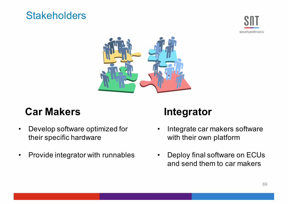
• Develop software optimized for their specific hardware

• Provide integrator with runnables

• Integrate car makers software with their own platform

• Deploy final software on ECUs and send them to car makers

Car Makers Integrator

Stakeholders

69

• Objective: Effective execution and synchronization of runnables

• Some runnables should execute simultaneously or in a certain order

• Objective: Effective usage of CPU time

• Max CPU time used by all the runnables should remain as low as possible over time

Car Makers Integrator

Different Objectives

70

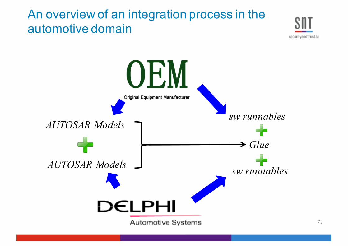
An overview of an integration process in the automotive domain

AUTOSAR Modelssw runnables

sw runnablesAUTOSAR Models

Glue

71

72

CPU time shortage

• Static cyclic scheduling: predictable, analyzable• Challenge

– Many OS tasks and their many runnables run within a limited available CPU time

• The execution time of the runnables may exceed their time slot

• Goal– Reducing the maximum CPU time used per time slot to be

able to• Minimize the hardware cost• Reduce the probability of overloading the CPU in practice• Enable addition of new functions incrementally

72

5ms 10ms 15ms 20ms 25ms 30ms 35ms 40ms

✗

5ms 10ms 15ms 20ms 25ms 30ms 35ms 40ms ✔

(a)

(b)

Fig. 4. Two possible CPU time usage simulations for an OS task with a 5mscycle: (a) Usage with bursts, and (b) Desirable usage.

its corresponding glue code starts by a set of declarationsand definitions for components, runnables, ports, etc. It thenincludes the initialization part followed by the execution part.In the execution part, there is one routine for each OS task.These routines are called by the scheduler of the underlyingOS in every cycle of their corresponding task. Inside eachOS task routine, the runnables related to that OS task arecalled based on their period. For example, in Figure 3, weassume that the cycle of the task o1 is 5ms, and the periodof the runnables r1, r2, and r3 are 10ms, 20ms and 100ms,respectively. The value of timer is the global system time. Sincethe cycle of o1 is 5, the value of timer in the Task o1() routineis always a multiple of 5. Runnables r1, r2 and r3 are thencalled whenever the value of timer is zero, or is divisible bythe period of r1, r2 and r3, respectively.

Although AUTOSAR provides a standard means for OEMsand suppliers to exchange their software, and essentiallyenables the process in Figure 1, the automotive integrationprocess still remains complex and erroneous. A major inte-gration challenge is to minimize the risk of CPU shortagewhile running the integrated system in Figure 1. Specifically,consider an OS task with a 5ms cycle. Figure 4 shows twopossible CPU time usage simulations of this task over eighttime slots between 0 to 40ms. In Figure 4(a), there are burstsof high CPU usage at two time slots at 0ms and 35ms, whilethe CPU usage simulation in Figure 4(b) is more stable anddoes not include any bursts. In both simulations, the totalCPU usage is the same, but the distribution of the CPU usageover time slots is different. The simulation in Figure 4(b) ismore desirable because: (1) It minimizes the hardware costsby lowering the maximum required CPU time. (2) It facilitatesthe assignment of new runnables to an OS task, and hence,enables the addition of new functions as it is typically done inthe incremental design of car manufacturers. (3) It reduces thepossibility of overloading CPU as the CPU time usage is lesslikely to exceed the OS task cycle (i.e., 5ms) in any time slot.Ideally, a CPU usage simulation is desirable if in each timeslot, there is a sufficiently large safety margin of unused CPUtime. Due to inaccuracies in estimating runnables’ executiontimes, it is expected that the unused margin shrinks when thesystem runs in a real car. Hence, the larger is this margin, thelower is the probability of exceeding the limit in practice.

In this paper, we study the problem of minimizing burstsof CPU time usage for a software system composed of alarge number of concurrent runnables. A known strategy toeliminate high CPU usage bursts is to shift the start time(offset) of runnables, i.e., to insert a delay prior to the start ofthe execution of runnables [5]. Offsets of the runnables mustsatisfy three constraints: C1. The offset values should not lead

to deadline misses, i.e., they should not cause the runnables torun passed their periods. C2. Since the runnables are invokedby OS tasks, the offset values of each runnable should bedivisible by the OS task cycle related to that runnable. C3. Theoffset values should not interfere with data dependency andsynchronization relations between runnables. For example,suppose runnables r1 and r2 have to execute in the same timeslot because they need to synchronize. The offset values of r1and r2 should be chosen such that they still run in the sametime slot after being shifted by their offsets.

There are four important context factors that are in line withAUTOSAR [13], and have influenced our work:

CF1. The runnables are not memory-bound, i.e., the CPUtime is not significantly affected by the low-bound memoryallocation activities such as transferring data in and out ofthe disk and garbage collection. Hence, our analysis of CPUtime usage is not affected by constraints related to memoryresources (see Section III-B).

CF2. The runnables are Offset-free [4], that is the offset ofa runnable can be freely chosen as long as it does not violatethe timing constraints C1-C3 (see Section III-B).

CF3. The runnables assigned to different OS tasks areindependent in the sense that they do not communicate withone another and do not share memory. Hence, the CPU timeused by an OS task during each cycle is not affected by otherOS tasks running concurrently. Our analysis in this paper,therefore, focuses on individual OS tasks.

CF4. The execution times of the runnables are remarkablysmaller than the runnables’ periods and the OS task cycles.Typical OS task cycles are around 1ms to 5ms. The runnables’periods are typically between 10ms to 1s, while the runnables’execution times are between 10ns = 10�5ms to 0.2ms.

Our goal is to compute offsets for runnables such that theCPU usage is minimized, and further, the timing constraints,C1-C3, discussed earlier above hold. This requires solvinga constraint-based optimization problem, and can be done inthree ways: (1) Attempting to predict optimal offsets in a de-terministic way, e.g., algorithms based on real-time schedulingtheory [6]. In general, these algorithms explore a very smallpart of the search space, i.e., worst/best case situations only(see Section V for a discussion). (2) Formulating the problemas a (symbolic) constraint model and applying a systematicconstraint solver [14], [15]. Due to assumption CF4 above,the search space in our problem is too large, resulting ina huge constraint model that does not fit in memory (seeSection V for more details). (3) Using metaheuristic search-based techniques [9]. These techniques are part of the generalclass of stochastic optimization algorithms which employsome degree of randomness to find optimal (or as optimalas possible) solutions to hard problems. These approaches areapplied to a wide range of problems, and are used in this paper.

III. SEARCH-BASED CPU USAGE MINIMIZATION

In this section, we describe our search-based technique forCPU usage minimization. We first define a notation for ourproblem in Section III-A. We formalize the timing constraints,

73

Using runnable offsets (delay times)

5ms 10ms 15ms 20ms 25ms 30ms 35ms 40ms

5ms 10ms 15ms 20ms 25ms 30ms 35ms 40ms ✗

✔

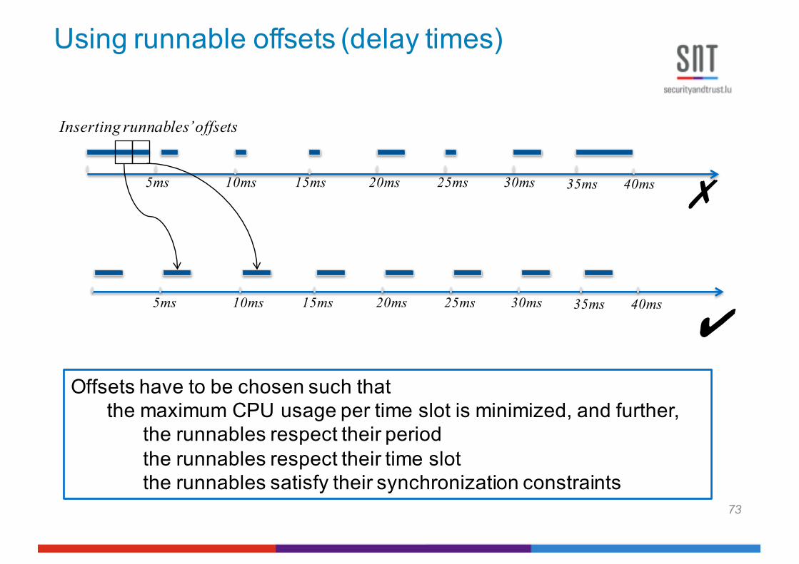
Inserting runnables’ offsets

Offsets have to be chosen such thatthe maximum CPU usage per time slot is minimized, and further,

the runnables respect their periodthe runnables respect their time slotthe runnables satisfy their synchronization constraints

73

5.34ms 5.34ms5 ms

Time

CPU

tim

e us

age

(ms)

CPU time usage exceeds the size of the slot (5ms)

Without optimization

74

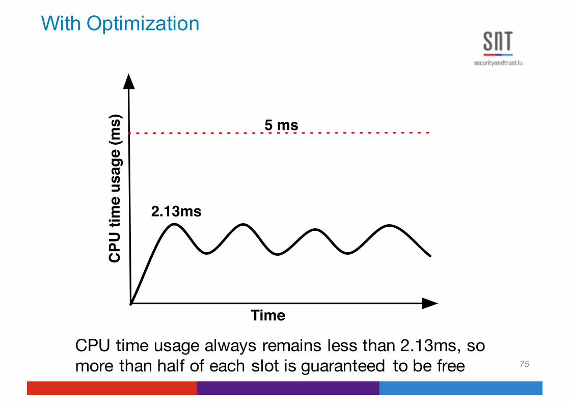
CPU time usage always remains less than 2.13ms, so more than half of each slot is guaranteed to be free

2.13ms

5 ms

Time

CPU

tim

e us

age

(ms)

With Optimization

75

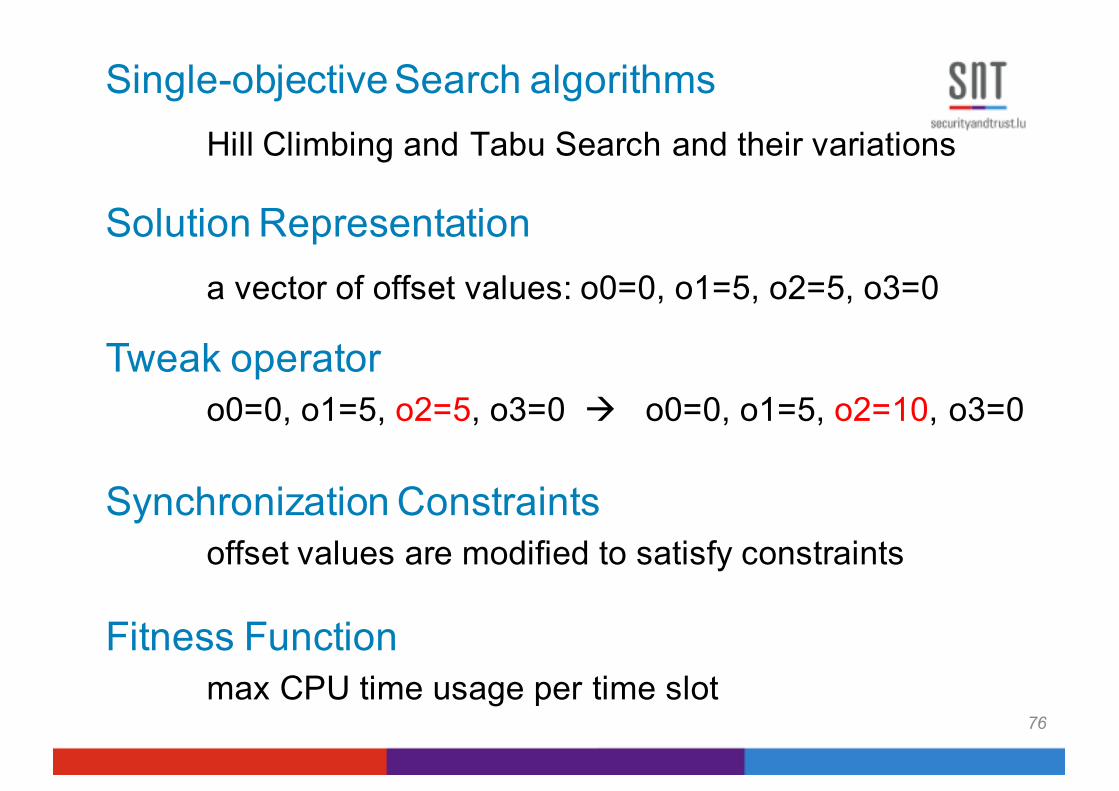
Single-objective Search algorithms Hill Climbing and Tabu Search and their variations

Solution Representationa vector of offset values: o0=0, o1=5, o2=5, o3=0

Tweak operatoro0=0, o1=5, o2=5, o3=0 à o0=0, o1=5, o2=10, o3=0

Synchronization Constraintsoffset values are modified to satisfy constraints

Fitness Functionmax CPU time usage per time slot

76

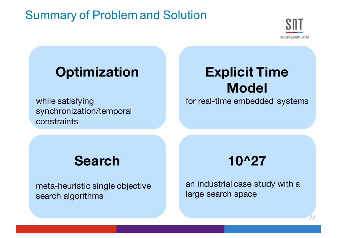
Summary of Problem and Solution

Optimization

while satisfying synchronization/temporal constraints

Explicit Time Model

for real-time embedded systems

Searchmeta-heuristic single objective search algorithms

10^27an industrial case study with a large search space

77

78

Search Solution and Results

Case Study: an automotive software system with 430 runnables, search space = 10^27

Running the system without offsets

Simulation for the runnables in our case study andcorresponding to the lowest max CPU usage found by HC

5.34 ms

Optimized offset assignment

2.13 ms

- The objective function is the max CPU usage of a 2s-simulation of runnables

- The search modifies one offset at a time, and updates other offsets only if timing constraints are violated

- Single-state search algorithms for discrete spaces (HC, Tabu)

78

79

Comparing different search algorithms

(ms)

(s)

Best CPU usage

Time to find Best CPU usage

79

80

Comparing our best search algorithm with random search

(a) (b) (c)(a)

Lowest max CPU usage values computed by HC within 70 msover 100 different runs

Lowest max CPU usage values computed by Random within 70 ms over 100 different runs

Comparing average behavior of Random and HC in computinglowest max CPU usage values within 70 s and over 100 different runs

80

HC Random Average

0ms 5ms 10ms 15ms 20ms 25ms 30ms

0ms 5ms 10ms 15ms 20ms 25ms 30ms

0ms 5ms 10ms 15ms 20ms 25ms 30ms4ms

3ms

2ms

Car Makers Integratorr0 r1 r2 r3

Minimize CPU time usage

1 slot

2 slots

3 slots

Execute r0 to r3 close to one another.

Trade-off between Objectives

81

Trade-off curve#

of s

lots

CPU time usage (ms) 2.041.45

12

21

14

1.56

1

23

Boundary Trade Offs

Interesting Solutions

82

Multi-objective search

• Multi-objective genetic algorithms (NSGA II)• Pareto optimality• Supporting decision making and negotiation between

stakeholders

83

Report: GraphRandom-NSGAII-25 Page 1 of 2

CPU Time Usage-NSGAII & CPU Time Usage-Random vs. Number of Slots-NSGAII & Number of Slots-Random

Number of Slots-NSGAII & Number of Slots-Random10 15 20 25 30 35 40 45 50

CPU

Tim

e U

sage

-NSG

AII &

CPU

Tim

e U

sage

-Ran

dom

1.5

2.0

2.5

3.0

3.5

Graph Builder

Total Number of Time Slots

Max

CPU

Tim

e U

sage

(ms)

Random(25,000)NSGA-II(25,000)

A

B

12

1.45

C

Objectives: • (1) Max CPU time • (2) Maximum time

slots between “dependent” tasks

Input.csv:- runnables- Periods- CETs- Groups- # of slots per

groups

SearchA list of solutions:- objective 1 (CPU usage)- objective 2 (# of slots)- vector of group slots- vector of offsets

Visualization/Query Analysis

- Visualize solutions- Retrieve/visualize

simulations- Visualize Pareto Fronts- Apply queries to the

solutions

Trade-Off Analysis Tool

84

85

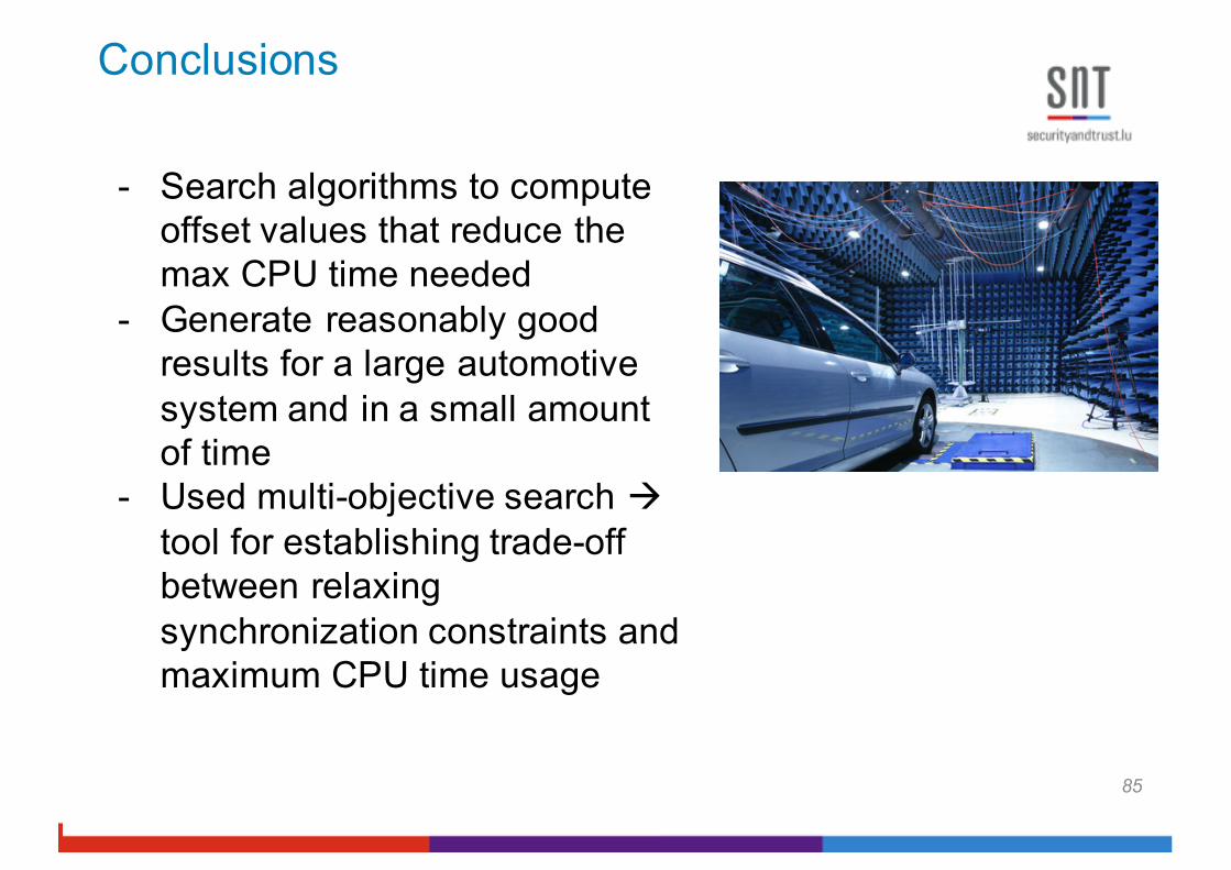
Conclusions

- Search algorithms to compute offset values that reduce the max CPU time needed

- Generate reasonably good results for a large automotive system and in a small amount of time

- Used multi-objective search àtool for establishing trade-off between relaxing synchronization constraints and maximum CPU time usage

85

Schedulability Analysis and Stress Testing

References:

86

• S. Di Alesio et al., “Worst-Case Scheduling of Software Tasks – A Constraint Optimization Model to Support Performance Testing, Constraint Programming (CP), 2014

• S. Di Alesio et al. “Combining Genetic Algorithms and Constraint Programming to Support Stress Testing”, ACM TOSEM, 25(1), 2015

Real-time, concurrent systems (RTCS)

• Real-time, concurrent systems (RTCS) have concurrent interdependent tasks which have to finish before their deadlines

• Some task properties depend on the environment, some are design choices

• Tasks can trigger other tasks, and can share computational resources with other tasks

• How can we determine whether tasks meet their deadlines?

87

Problem

• Schedulability analysis encompasses techniques that try to predict whether all (critical) tasks are schedulable, i.e., meet their deadlines

• Stress testing runs carefully selected test cases that have a high probability of leading to deadline misses

• Stress testing is complementary to schedulabilityanalysis

• Testing is typically expensive, e.g., hardware in the loop

• Finding stress test cases is difficult

88

Finding Stress Test Cases is Difficult

89

0123456789

j0, j1 , j2 arrive at at0 , at1 , at2 and must finish before dl0 , dl1 , dl2

J1 can miss its deadline dl1 depending on when at2 occurs!

0123456789

j0 j1 j2 j0 j1 j2at0

dl0

dl1

at1 dl2

at2

T

T

at0

dl0 dl1

at1at2

dl2

Challenges and Solutions

• Ranges for arrival times form a very large input space

• Task interdependencies and properties constrain what parts of the space are feasible

• We re-expressed the problem as a constraint optimisation problem

• Constraint programming (e.g., IBM CPLEX)

90

Constraint Optimization

91

Constraint Optimization Problem

Static Properties of Tasks(Constants)

Dynamic Properties of Tasks(Variables)

Performance Requirement(Objective Function)

OS Scheduler Behaviour(Constraints)

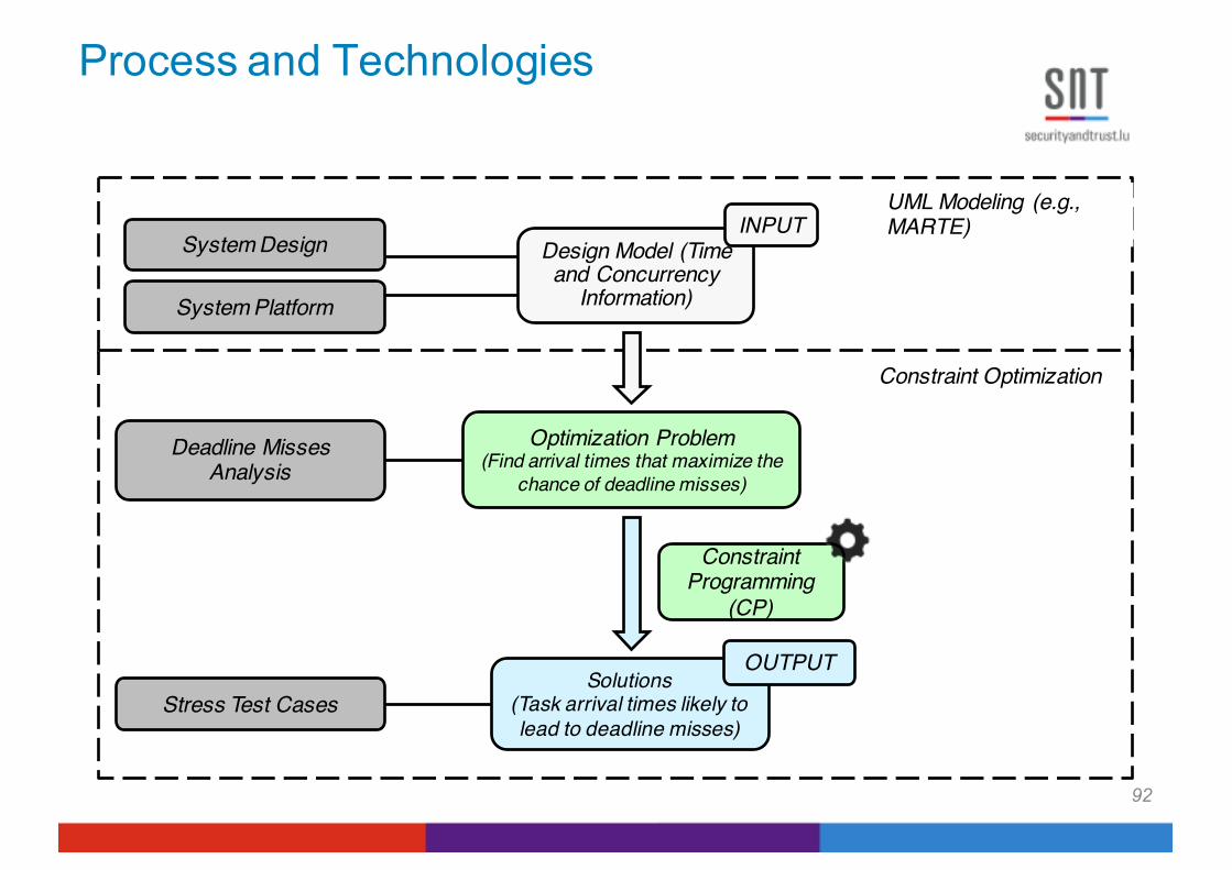
Process and Technologies

92

UML Modeling (e.g., MARTE)


Optimization Problem(Find arrival times that maximize the

chance of deadline misses)

System Platform

Solutions(Task arrival times likely to lead to deadline misses)

Deadline Misses Analysis

System Design Design Model (Time and Concurrency

Information)

INPUT

OUTPUT

Stress Test Cases

Constraint Programming

(CP)

Context

93

Drivers(Software-Hardware Interface)

Control Modules

Alarm Devices(Hardware)

Multicore Architecture

Real-Time Operating System

System monitors gas leaks and fire in oil extraction platforms

Challenges and Solutions

• CP effective on small problems• Scalability problem: Constraint programming (e.g.,

IBM CPLEX) cannot handle large input spaces (CPU, memory)

• Solution: Combine metaheuristic search and constraint programming– metaheuristic search (GA) identifies high risk regions in the

input space – constraint programming finds provably worst-case schedules

within these (limited) regions– Achieve (nearly) GA efficiency and CP effectiveness

• Our approach can be used both for stress testing and schedulability analysis (assumption free)

94

Combining GA and CP

95

A:12 S. Di Alesio et al.

Fig. 3: Overview of GA+CP: the solutions x1, y1 and z1 in the initial population of GA evolve intox6, y6, and z6, then CP searches in their neighborhood for the optimal solutions x⇤, y⇤ and z

⇤.

in the schedule generated by the arrival times in x:

J

⇤(x)

def=

n

j 2 J

�

� 9k⇤ 2 K

j

⇤(x) ·

�

deadline miss

j

⇤,k

⇤(x) � 0 _

8j 2 J, k 2 K

j

·

deadline miss

j

⇤,k

⇤(x) � deadline miss

j,k

(x)

�

o

— Union set I⇤ of impacting sets of tasks missing or closest to miss their deadlines. Let I⇤(x)be the union of the impacting sets of tasks in J

⇤(x):

I

⇤(x)

def=

[

j

⇤2J

⇤(x)

I

j

⇤(x)

By definition, I⇤(x) contains all the tasks that can have an impact over a task that misses adeadline or is closest to a deadline miss.

— Neighborhood ✏ of an arrival time and neighborhood size D. Let ✏(xj,k

) be the intervalcentered in the arrival time x

j,k

computed by GA, and let D be its radius: ✏(xj,k

) = [x

j,k

�D, x

j,k

+D]. ✏ defines the part of the search space around x

j,k

where to find arrival times thatare likely to break task deadlines. D is a parameter of the search.

— Constraint Model M implementing a Complete Search Strategy. Let M be the constraintmodel defined in our previous work [Di Alesio et al. 2014] for the purpose of identifying ar-rival times for tasks that are likely to lead to deadline misses scenarios. M models the staticand dynamic properties of the software system respectively as constants and variables, and thescheduler of the operating system as a set of constraints among such variables. Note that M im-plements a complete search strategy over the space of arrival times. This means that M searchesfor arrival times of all aperiodic tasks within the whole interval T .

Our combined GA+CP strategy consists in the following two steps:

ACM Transactions on Software Engineering and Methodology, Vol. V, No. N, Article A, Pub. date: January YYYY.

Process and Technologies

96

UML Modeling (e.g., MARTE)


Optimization Problem(Find arrival times that maximize the

chance of deadline misses)

System Platform

Solutions(Task arrival times likely to lead to deadline misses)

Deadline Misses Analysis

System Design Design Model (Time and Concurrency

Information)

INPUT

OUTPUT

Genetic Algorithms

(GA)

Stress Test Cases

Constraint Programming

(CP)

V&V Topics Addressed by Search

• Many projects over the last 15 years

• Design-time verification– Schedulability– Concurrency – Resource usage

• Testing– Stress/load testing, e.g., task deadlines– Robustness testing, e.g., data errors– Reachability of safety or business critical states, e.g.,

collision and no warning– Security testing, e.g., XML and SQLi injections

97

Publicity!

• Chunhui Wang et al., “System Testing of Timing Requirements based on Use Cases and Timed Automata”. Session R09 @ ICST 2017, Tuesday, 2 pm

• Sadeeq Jan et al., “A Search-based Testing Approach for XML Injection Vulnerabilities in Web Applications”. Session R11 @ ICST 2017, Thursday 11 am

98

99

Objective Function

Search Space

Search Technique

n Problem = fault modeln Model = system or

environmentn Search to optimize

objective function(s) n Metaheuristicsn Scalability: A small part

of the search space is traversed

n Model: Guidance to worst case, high-risk scenarios across space

n Reasonable modeling effort based on standards or extension

n Heuristics: Extensive empirical studies are required

General Pattern: Using Metaheuristic Search

100

Objective Function

Search Space

Search Technique

n Model simulation can be time consuming

n Makes the search impractical or ineffective

n Surrogate modeling based on machine learning

n Simulator dedicated to search


Simulator

101

Objective Function

Search Space

Search Technique

n Use techniques such as sensitivity analysis to minimize dimensionality before running search

n Predict parts of the space worth searching in


Large

102

Objective Function

Search Space

Search Technique

n Combine with solvers and optimization engines

n Need heuristic strategies to determine when to use what


Multiple techniques?

Scalability

103

Project examples

• Scalability is the most common verification challenge in practice

• Testing closed-loop controllers, DA system– Large input and configuration space– Expensive simulations– Smart heuristics to avoid simulations (machine learning

to predict fitness)• Schedulability analysis and stress testing

– Large space of possible arrival times– Constraint programming cannot scale by itself– CP was carefully combined with genetic algorithms

104

Scalability: Lessons Learned

• Scalability must be part of the problem definition and solution from the start, not a refinement or an after-thought

• Meta-heuristic search, by necessity, has been an essential part of the solutions, along with, in some cases, machine learning, statistics, etc.

• Scalability often leads to solutions that offer “best answers” within time constraints, but no guarantees

• Scalability analysis should be a component of every research project – otherwise it is unlikely to be adopted in practice

• How many papers research papers do include even a minimal form of scalability analysis?

105

Practicality

106

Project examples

• Practicality requires to account for the domain and context

• Testing controllers– Relies on Simulink only– No additional modeling or complex translation– Differences between open versus closed loop

controllers• Minimizing risks of CPU shortage

– Trade-off between between effective synchronization and CPU usage

– Trade-off achieved through multiple-objective GA search and appropriate decision tool

107

Practicality: Lessons Learned

• In software engineering, and verification in particular, just understanding the real problems in context is difficult

• What are the inputs required by the proposed technique?

• How does it fit in development practices?• Is the output what engineers require to make

decisions?• There is no unique solution to a problem as they tend

to be context dependent, but a context is rarely unique and often representative of a domain or type of system

108

Discussion

• Metaheuristic search for verification and testing– Tends to be versatile, tailorable to new problems and

contexts– Particularly suited to the verification of non-functional

properties– Entails acceptable modeling requirements– Can provide “best” answers at any time– Scalable, practical

But– Not a proof, no certainty– Effectiveness of search guidance is key and must be

experimentally evaluated– Models are key to provide adequate guidance– Search must often be combined with other techniques, e.g.,

machine learning, constraint programming 109

Discussion II

• Constraint solvers (e.g., Comet, ILOG CPLEX, SICStus)– Is there an efficient constraint model for the problem at hand?– Can effective heuristics be found to order the search?– Better if there is a match to a known standard problem, e.g., job

shop scheduling– Tend to be strongly affected by small changes in the problem, e.g.,

allowing task pre-emption– Often not scalable, e.g., memory

• Model checking– Detailed operational models (e.g., state models), involving

(complex) temporal properties (e.g., CTL)– Enough details to analyze statically or execute symbolically – These modeling requirements are usually not realistic in actual

system development. State explosion problem. – Originally designed for checking temporal properties through

reachability analysis, as opposed to explicit timing properties– Often not scalable 110

Talk Summary

• Focus: Meta-heuristic Search to enable scalable verification and testing.

• Scalability is the main challenge in practice.• We drew lessons learned from example projects in

collaboration with industry, on real systems and in real verification contexts.

• Results show that meta-heuristic search contributes to mitigate the scalability problem.

• It has also shown to lead to practical solutions.• Solutions are very context dependent.• Solutions tend to be multidisciplinary: system modeling,

constraint solving, machine learning, statistics. 111

Acknowledgements

PhD. Students: • Vahid Garousi• Marwa Shousha• Zohaib Iqbal• Reza Matinnejad• Stefano Di Alesio• Raja Ben Abdessalem

Scientists:• Shiva Nejati• Andrea Arcuri

112

Scalable Software Testing and Verification of Non-Functional Properties through

Heuristic Search and Optimization

Lionel Briand

Interdisciplinary Centre for ICT Security, Reliability, and Trust (SnT)University of Luxembourg, Luxembourg

ITEQS, March 13, 2017

SVV lab: svv.luSnT: www.securityandtrust.lu

We are hiring!