Embed Size (px)
Citation preview

Khawar Khurshid, 20121
Advanced Digital Image Processing
Spring ’14

Intensity TransformationsIntensity TransformationsIntensity TransformationsIntensity Transformations
LookLookLookLook----up Tablesup Tablesup Tablesup Tables
Linear Contrast StretchLinear Contrast StretchLinear Contrast StretchLinear Contrast Stretch
PiecePiecePiecePiece----wise Contrast Stretchwise Contrast Stretchwise Contrast Stretchwise Contrast Stretch
Histogram EqualizationHistogram EqualizationHistogram EqualizationHistogram Equalization
Power LawPower LawPower LawPower Law
Log Transform Log Transform Log Transform Log Transform –––– Gamma correctionGamma correctionGamma correctionGamma correction
Khawar Khurshid, 20122

Dynamic Range Dynamic Range Dynamic Range Dynamic Range vsvsvsvs ContrastContrastContrastContrast
Khawar Khurshid, 2012
Dynamic Range Minimum Possible Intensity to Maximum Possible Intensity
Contrast Minimum Image Intensity to Maximum Image Intensity
What do you think is the dynamic range of this image?
What is the approximate contrast range?
3

� Point/Pixel operationsOutput value at specific coordinates(x,y) is dependent only on the inputvalue at (x,y)
� Local operationsThe output value at (x,y) isdependent on the input values in theneighborhood of (x,y)
�Global operationsThe output value at (x,y) isdependent on all the values in theinput image
Intensity TransformationsIntensity TransformationsIntensity TransformationsIntensity Transformations
Khawar Khurshid, 20124

Basic Concept
Most spatial domain enhancement operations can be generalized as:
f (x, y) = Input image
g (x, y) = Processed/output image
T = Operator defined over some neighbourhood of (x, y)
[ ]( , ) ( , )g x y T f x y=
Intensity TransformationsIntensity TransformationsIntensity TransformationsIntensity Transformations
Khawar Khurshid, 20125

Point Processing using Look-up Tables
ce
ll in
de
x
co
nte
nts
0 0
64 32
128 128
192 224
255 255
...
...
...
...
...
...
...
...
input output
a pixel with this value
a pixel with this value
is mapped to this value
is mapped to this value
Look up Table MappingLook up Table MappingLook up Table MappingLook up Table Mapping
Khawar Khurshid, 20126

Linear Contrast StretchLinear Contrast StretchLinear Contrast StretchLinear Contrast Stretch
Khawar Khurshid, 20127

� Objective� Increase the dynamic
range of the gray levelsfor low contrast images
� Rather than using a well
defined mathematical
function we can use
arbitrary user-defined
transforms
� If r1 = s1 & r2 = s2, no change in gray levels
� If r1 = r2, s1 = 0 & s2 = L-1, then it is a threshold function. The resulting image is binary
PiecePiecePiecePiece----wise Contrast Stretchingwise Contrast Stretchingwise Contrast Stretchingwise Contrast Stretching
Khawar Khurshid, 20128

PiecePiecePiecePiece----wise Contrast Stretchingwise Contrast Stretchingwise Contrast Stretchingwise Contrast Stretching
Khawar Khurshid, 20129
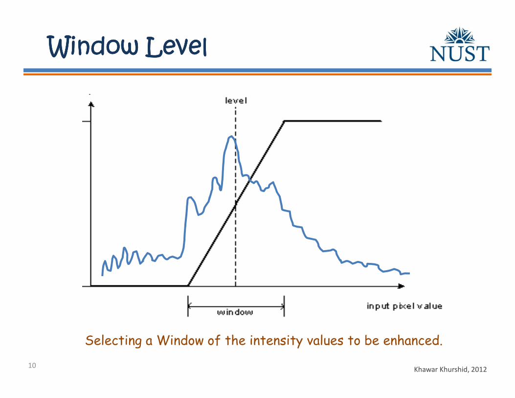
Window LevelWindow LevelWindow LevelWindow Level
Khawar Khurshid, 2012
Selecting a Window of the intensity values to be enhanced.
10

Window LevelWindow LevelWindow LevelWindow Level
Khawar Khurshid, 2012
Window of dark intensity values are enhanced.
11

Window LevelWindow LevelWindow LevelWindow Level
Khawar Khurshid, 2012
Intensity values corresponding to the Lungs is enhanced.
12
HistogramHistogramHistogramHistogramOfOfOfOf
ImagesImagesImagesImages
Khawar Khurshid, 201213

• The histogram of a digital image with gray values is the discrete function
• Nk : Number of pixels with gray value rk
• N : Total number of pixels in the image
• The function p(rk) represents the fraction of the total number of pixels with gray value rk.
n
nrp k
k =)( 1,...,1,0 −= Lk
Image Histogram Image Histogram Image Histogram Image Histogram
Khawar Khurshid, 201214

0 1 1 2 4
2 1 0 0 2
5 2 0 0 4
1 1 2 4 1
The (intensity or brightness) histogram shows how many times a particular grey level (intensity) appears in an image.
For example, 0 - black, 255 – white
0
1
2
3
4
5
6
7
0 1 2 3 4 5 6
Image Histogram
Image Histogram Image Histogram Image Histogram Image Histogram
Khawar Khurshid, 201215

I = imread('rain.jpg');
G = rgb2gray(I);
[x,y] = size(G);
H = zeros(1,256);
for i=1:x
for j=1:y
H(G(i,j)+1) = H(G(i,j)+1) + 1;
end
end
stem(H);
Histogram CalculationHistogram CalculationHistogram CalculationHistogram Calculation
Khawar Khurshid, 201216

( ) the number
of pixels in
with graylevel .
Ih g
I
g
=( ) the number
of pixels in
with graylevel .
Ih g
I
g
=
Histogram Histogram Histogram Histogram –––– Gray Scale ImageGray Scale ImageGray Scale ImageGray Scale Image
Khawar Khurshid, 201217

There is one histo-gram per color bandR, G, & B. Luminosity histogram is from 1 band = (R+G+B)/3
There is one histo-gram per color bandR, G, & B. Luminosity histogram is from 1 band = (R+G+B)/3
Histogram Histogram Histogram Histogram –––– Color ImageColor ImageColor ImageColor Image
Khawar Khurshid, 201218

Histogram Histogram Histogram Histogram –––– Color ImageColor ImageColor ImageColor Image
Khawar Khurshid, 201219

Histogram EqualizationHistogram EqualizationHistogram EqualizationHistogram Equalization
Khawar Khurshid, 201220

The CDF (cumulative distribution) is the LUT for remapping.
The CDF (cumulative distribution) is the LUT for remapping.
CDF
Histogram EqualizationHistogram EqualizationHistogram EqualizationHistogram Equalization
Khawar Khurshid, 201221

The CDF (cumulative distribution) is the LUT for remapping.
The CDF (cumulative distribution) is the LUT for remapping.
LUT
Histogram EqualizationHistogram EqualizationHistogram EqualizationHistogram Equalization
Khawar Khurshid, 201222

Histogram Equalization Histogram Equalization Histogram Equalization Histogram Equalization ---- LocalLocalLocalLocal
Khawar Khurshid, 2012
Original Image Local EqualizationGlobal Equalization
23

Histogram Equalization istogram Equalization istogram Equalization istogram Equalization ---- ProblemProblemProblemProblem
Khawar Khurshid, 2012Problem with Histogram Equalization
24

� Power law transformations have the following form
� Map a narrow range of dark input values into a wider range of output values or vice versa
� Varying γ gives a whole family of curves
s c rγ= ×
Power Law Power Law Power Law Power Law TransformationsTransformationsTransformationsTransformations
Khawar Khurshid, 201225
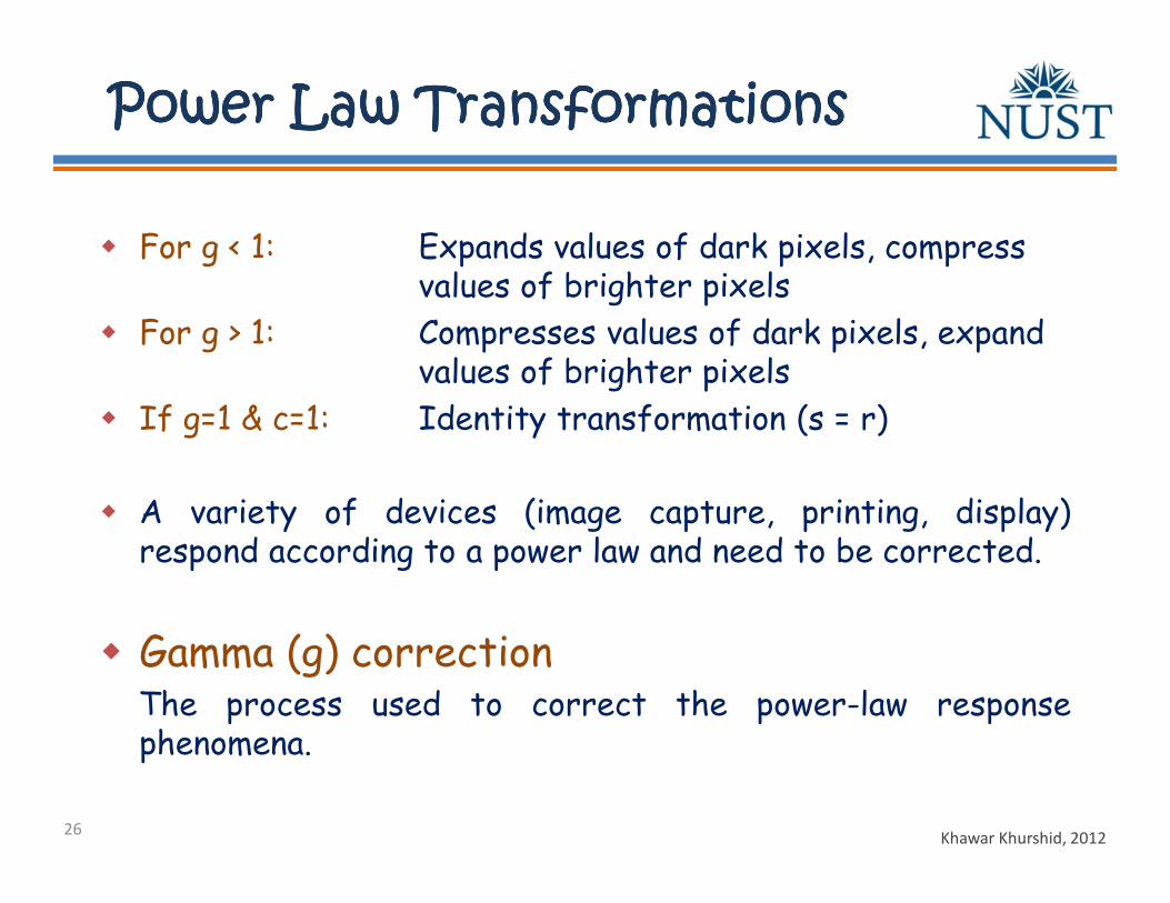
� For g < 1: Expands values of dark pixels, compress values of brighter pixels
� For g > 1: Compresses values of dark pixels, expand values of brighter pixels
� If g=1 & c=1: Identity transformation (s = r)
� A variety of devices (image capture, printing, display)respond according to a power law and need to be corrected.
� Gamma (g) correctionThe process used to correct the power-law responsephenomena.
Power Law Power Law Power Law Power Law TransformationsTransformationsTransformationsTransformations
Khawar Khurshid, 201226

MR image of
human spine
Result after
Power law
transformation
γγγγ = 0.6
Result after
Power law
transformation
γγγγ = 0.4
Result after
Power law
transformation
γγγγ = 0.3
Power Law TransformationsPower Law TransformationsPower Law TransformationsPower Law Transformations
Khawar Khurshid, 201227

Image has a washed-outappearance – needs γ > 1
Power Law Power Law Power Law Power Law TransformationsTransformationsTransformationsTransformations
Khawar Khurshid, 201228

Aerial
Image
Result of
Power law
transformation
γγγγ = 3.0
(suitable)
Result of
Power law
transformation
γγγγ = 4.0
(suitable)
Result of
Power law
transformation
γγγγ = 5.0
(high contrast,
some regions are
too dark)
Power Law Power Law Power Law Power Law TransformationsTransformationsTransformationsTransformations
Khawar Khurshid, 201229

� The general form of the log transformation is
� The log transformation maps a narrow range of low input grey level values into a wider range of output values
� The inverse log transformation performs the opposite transformation
log(1 )s c r= × +
Logarithmic TransformationsLogarithmic TransformationsLogarithmic TransformationsLogarithmic Transformations
Khawar Khurshid, 201230

� Properties
� For lower amplitudes ofinput image the range ofgray levels is expanded.
� For higher amplitudes ofinput image the range ofgray levels is compressed.
Logarithmic TransformationsLogarithmic TransformationsLogarithmic TransformationsLogarithmic Transformations
Khawar Khurshid, 201231

Negative of an image?
Intensity Slicing?
Intensity TransformationsIntensity TransformationsIntensity TransformationsIntensity Transformations
Khawar Khurshid, 201232

Orientation EffectOrientation EffectOrientation EffectOrientation Effect
Khawar Khurshid, 201233

Orientation EffectOrientation EffectOrientation EffectOrientation Effect
Khawar Khurshid, 201234

Khawar Khurshid, 201235
EndIntensity Transformations