Embed Size (px)
Citation preview

Automated Parameterization of Performance Models from Measurements Giuliano Casale Imperial College London, UK Simon Spinner University of Würzburg, Germany Weikun Wang Imperial College London, UK Tutorial @ ICPE 2016, Delft, the Netherlands, March 13, 2016

2
Workload Characterization Common parameters in performance models: Service demand of a request CPU time, bandwidth consumed, …
Arrival rate of requests
Applications Automated performance modelling Resource cost splitting Performance anomaly detection …

3
Example: Queueing Modelling
Demands
Java Modelling Tools: http://jmt.sf.net

4
Example: Cost Splitting Carico Workload 1
Tran
sazi
oni/o
ra
Lun Mar Mer Gio Ven Sab Dom
010
020
030
040
0
Carico Workload 2
Tran
sazi
oni/o
ra
050
150
250
Lun Mar Mer Gio Ven Sab Dom
Ripartizione dei Costi
Util
izzo
CP
U -
%
020
4060
8010
0
Lun Mar Mer Gio Ven Sab DomCarico Workload 3
Tran
sazi
oni/o
ra
050
100
150
200
Lun Mar Mer Gio Ven Sab Dom
Workload 1
Workload 2
Workload 3
# Tr
ansa
ctio
ns
# Tr
ansa
ctio
ns
# Tr
ansa
ctio
ns
Mo Tu We Th Fr Sa Su
Mo Tu We Th Fr Sa Su
Mo Tu We Th Fr Sa Su
Mo Tu We Th Fr Sa Su
How to recover weight of individual contributions to utilization?
Util
izat
ion
[0-1
00%
]
We know from theory that the weight is exactly the service demand!

5
A Typical Challenge
5
HTTP Requests in the WS (Web Server)
Observation period T
1 request in WS
3 requests in WS
0 requests in WS
Time

6
A Typical Challenge OS schedules jobs in round robin If n requests run simultaneously, each will approximately receive 1/n of the CPU time Process Sharing is a round robin where the quantum of time assigned to each request is infinitesimal
6
X X
Service time S of the yellow request
Time
CPU
33% CPU time each
50% each
100% for blue
X
Quantum
Requests Arrive
Simultaneously
3 requests running

7
Tutorial Agenda
Introduction Demand Estimation Utilization-based
– LibReDE tool Response-based Queue Length-based
– FG tool Comparison Study & Case Studies Arrival Rate Estimation
– M3A tool

1
Demand Estimation

2
Overview Estimation Approaches (first part) Simple Utilization Response Time
LibReDE demo Estimation Approaches (second part) Queue Length

3
Response Time Approximation
Trivial approximation: 𝐷𝐷𝑖𝑖,𝑐𝑐 ≈ 𝑅𝑅𝑐𝑐 Assumptions resource dominates system response time waiting time in queue ≪ 𝐷𝐷𝑖𝑖,𝑐𝑐
Only applicable at low resource utilization

4
Service Demand Law Basic operational law:
𝐷𝐷𝑖𝑖,𝑐𝑐 =𝑈𝑈𝑖𝑖,𝑐𝑐𝑋𝑋0,𝑐𝑐
Partial utilization 𝑈𝑈𝑖𝑖,𝑐𝑐 is hard to derive Operating system: per-process statistics Profilers: high-overheads
2 alternative solutions: Controlled experiment Partitioning

5
Controlled Experiment Measurement Interval CPU Utilization Requests executed in separate experiments Resource Demand Problems: Not applicable at runtime Mutual interference
40%
Request1
30%
Request2

6
Partitioning Measurement Interval CPU Utilization Mixed Workload How to partition processing time? Response times Additional performance counters
60%
Request2
Request1 ?

7
Estimation Approaches
Data Collection Data Collection
Demand Estimation
Demand Estimation
Modeling Assumptions (scheduling, service distribution)
Modeling Assumptions (scheduling, service distribution)
Model Solution Model Solution
Utilization Approach Response Time Approach

8
Linear Regression Linear model (based on Utilization Law) 𝑈𝑈𝑖𝑖 = ∑ 𝑋𝑋𝑖𝑖,𝑐𝑐𝑁𝑁
𝑐𝑐 ∙ 𝐷𝐷𝑖𝑖,𝑐𝑐 + 𝑈𝑈0 Example:
At least 𝑚𝑚 > 𝑛𝑛 observations required Alternative solutions: Least-Squares Regression Least Absolute Differences Regression …
0.54 = 3 * 𝐷𝐷𝑖𝑖,1 + … + 8 * 𝐷𝐷𝑖𝑖,𝑛𝑛 0.72 = 9 * 𝐷𝐷𝑖𝑖,1 + … + 4 * 𝐷𝐷𝑖𝑖,𝑛𝑛 0.33 = 2 * 𝐷𝐷𝑖𝑖,1 + … + 9 * 𝐷𝐷𝑖𝑖,𝑛𝑛 … = …

9
Example: Outliers
Outliers can bias the regression
Fit Without Outliers
10
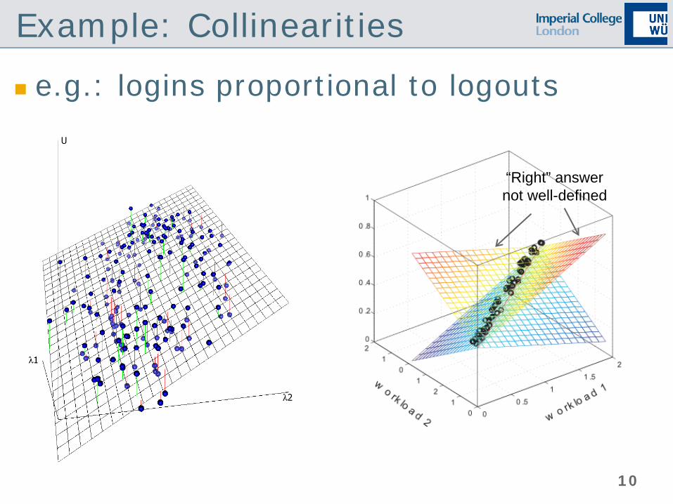
Example: Collinearities
e.g.: logins proportional to logouts
“Right” answer not well-defined

11
Other Approaches Robust regression Least Absolute Differences: Zhang et al. (2007) Least Trimmed Squares: Casale et al. (2008)
Machine-learning Clusterwise linear regression: Cremonesi et al. (2010) Pattern matching: Cremonesi et al. (2014)
12
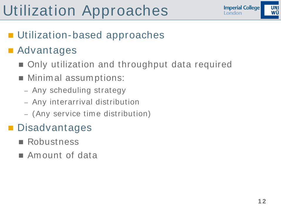
Utilization Approaches Utilization-based approaches Advantages Only utilization and throughput data required Minimal assumptions:
– Any scheduling strategy – Any interarrival distribution – (Any service time distribution)
Disadvantages Robustness Amount of data

13
Response Time Approaches Assumptions Single queue: closed-form solution exists Queueing network: product-form
Response time equations depend on Scheduling strategy Service distribution Interarrival time distribution
If M/G/1 with PS or LCFS or M/M/1 with FCFS and class-independent service
times, then 𝑅𝑅 = 𝐷𝐷1−𝑈𝑈

14
General Optimization Assumptions: Variables 𝑫𝑫 = (𝐷𝐷1,1, … ,𝐷𝐷1,𝑛𝑛, … ,𝐷𝐷𝑖𝑖,1, … ,𝐷𝐷𝑖𝑖,𝑛𝑛) Queueing Network QN 𝒛𝒛 = 𝑓𝑓(𝑫𝑫) Observation data 𝒛𝒛�
Optimization Problem: min
𝑫𝑫𝒛𝒛 − 𝒛𝒛�
𝑫𝑫 may be subject to certain constraints
arbitrary norm

15
Examples Menascé (2008): Liu et al. (2006):
Squared response time error Product-form solution (non-linear!)
Constrained to valid solutions
16
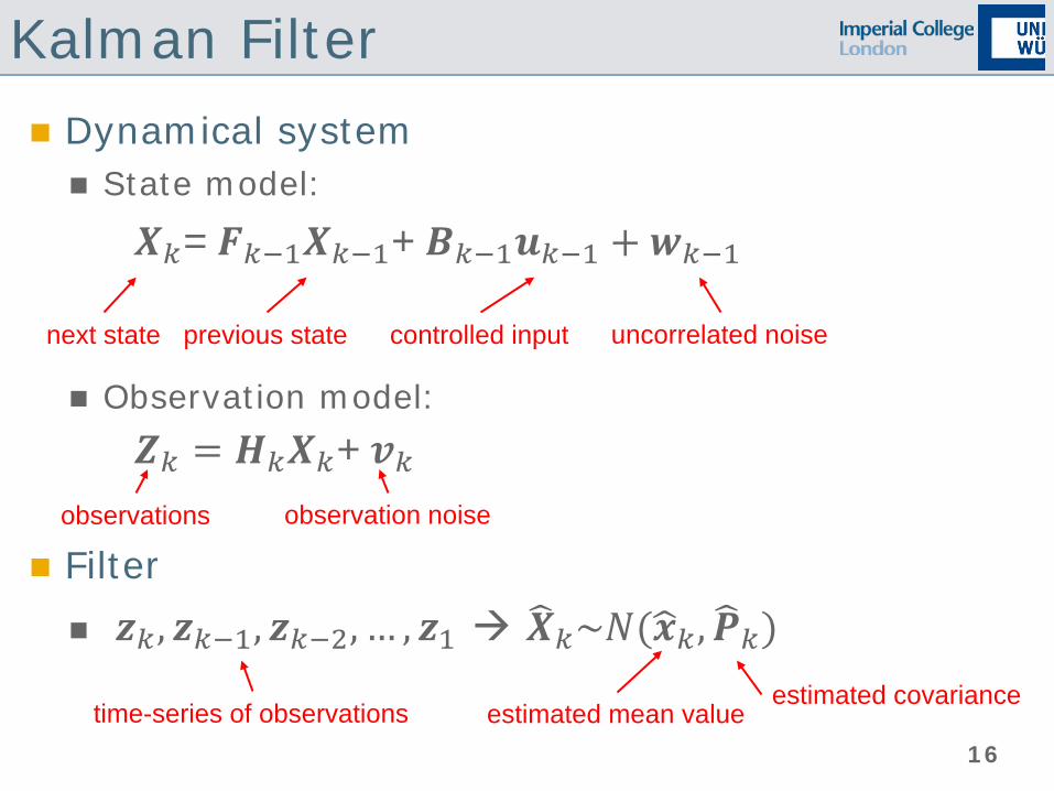
Kalman Filter Dynamical system State model:
𝑿𝑿𝑘𝑘=𝑭𝑭𝑘𝑘−1𝑿𝑿𝑘𝑘−1+𝑩𝑩𝑘𝑘−1𝒖𝒖𝑘𝑘−1 + 𝒘𝒘𝑘𝑘−1 Observation model:
𝒁𝒁𝑘𝑘 = 𝑯𝑯𝑘𝑘𝑿𝑿𝑘𝑘+𝒗𝒗𝑘𝑘 Filter 𝒛𝒛𝑘𝑘 , 𝒛𝒛𝑘𝑘−1, 𝒛𝒛𝑘𝑘−2, … , 𝒛𝒛1 𝑿𝑿�𝑘𝑘~𝑁𝑁(𝒙𝒙�𝑘𝑘,𝑷𝑷�𝑘𝑘)
observations
previous state controlled input uncorrelated noise next state
estimated mean value estimated covariance
time-series of observations
observation noise

17
Applied to Demand Estimation
State vector 𝑿𝑿𝑘𝑘 = 𝑫𝑫 Constant state model 𝑿𝑿𝑘𝑘=𝑿𝑿𝑘𝑘−1 + 𝒘𝒘𝑘𝑘−1 Observation model (e.g., Kumar et al. 2009)
𝑅𝑅1⋮𝑈𝑈
=
𝐷𝐷11 − 𝑈𝑈⋮
𝑋𝑋1 ∙ 𝐷𝐷1 + ⋯+ 𝑋𝑋𝐶𝐶 ∙ 𝐷𝐷𝑐𝑐
Other observation models are possible (e.g., Zheng et al. 2008, Wang et al. 2012)

18
Want to learn more?
Elsevier PEVA, October 2015.
1
Response Time Based Estimation
Joint work with S. Kraft and S. Pacheco-Sanchez (SAP Belfast,
UK) and Juan F. Pérez (U. Melbourne, Australia)

2
Paradigm Shift
Demand Estimation
Modeling Assumptions
(Scheduling, Service Distribution)
Model Generation and Solution
Data Collection
Demand Estimation
Modeling Assumptions
(Scheduling, Service Distribution)
Model Generation and Solution
Data Collection
Utilization Approach Response Time Approach

3
Estimate demand D from response time R
We investigate the likelihood function in First-Come First-Served (FCFS) queues
– e.g., admission control, disk drive buffers, … Processor Sharing (PS) queues
– e.g., CPUs, bandwidth sharing, …
Observation
R D4 D3
D1
D2 D0
1. For each observed R sample 2. Draw D from parameter space 3. Compute likelihood P[R|D] 4. Move in parameter space to
maximize P[R|D]
Parameter Space
Maximum Likelihood Estimator

4
Model response time using absorbing CTMCs Under FCFS, future arrivals do not affect response time distribution of the tagged job
RT Likelihood in FCFS queues
D1 D2 D2 D1 D1
nK, jobs of class k in queue
D1 D1 1 2
3
4 5
1
Abs
orbi
ng tr
ansi
tion
Model State Space of Markov Chain 2
1
D1 D2 D2 D1 D1
3
D1 D2 D2
4
D2 D2
5
D2
1

5
RT Likelihood in FCFS queues
Probability of being absorbed by time t into a give CTMC state Well-understood: PH-type distributed FCFS Example:
Backlog seen upon arrival
Class 1 arrival
ML Problem (K classes)

6
Monitoring dataset Active mix: (1 ,2 ,1 ,1 , 0 ) Admission state (mix) and response times
Assumptions
V CPUs
R Classes + Class switching
W Workers
… Admission
Response time
Multi-core server
7
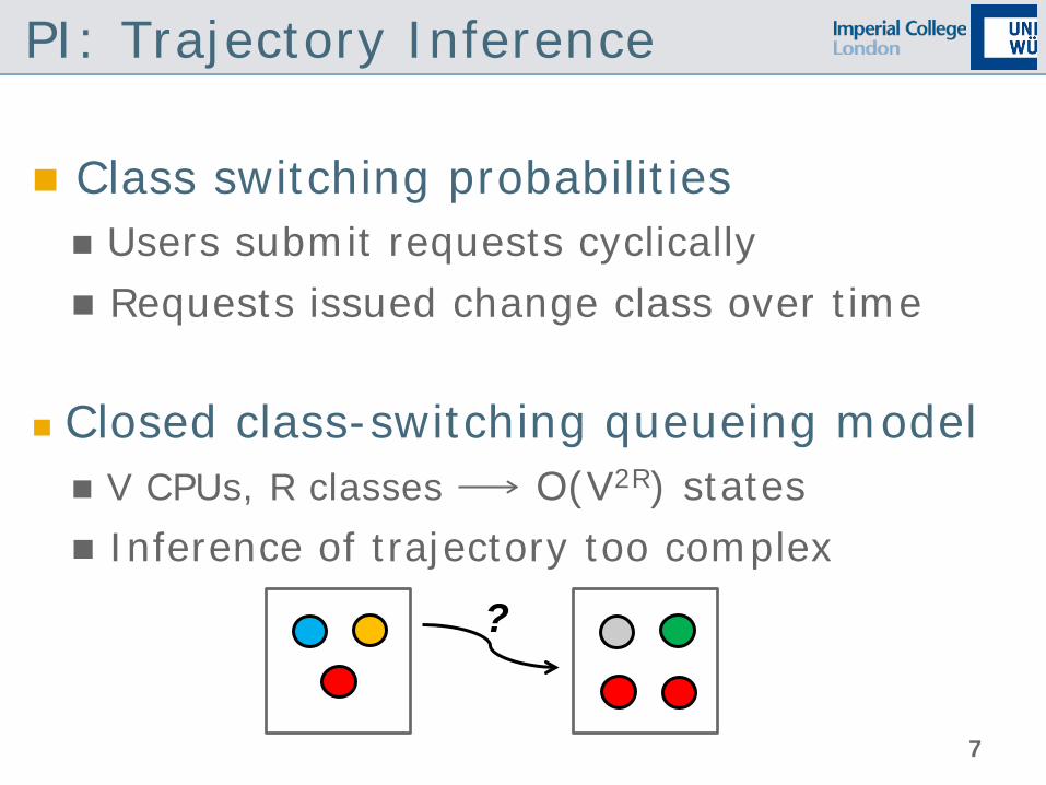
PI: Trajectory Inference
Class switching probabilities Users submit requests cyclically Requests issued change class over time
Closed class-switching queueing model V CPUs, R classes O(V2R) states Inference of trajectory too complex
?
8
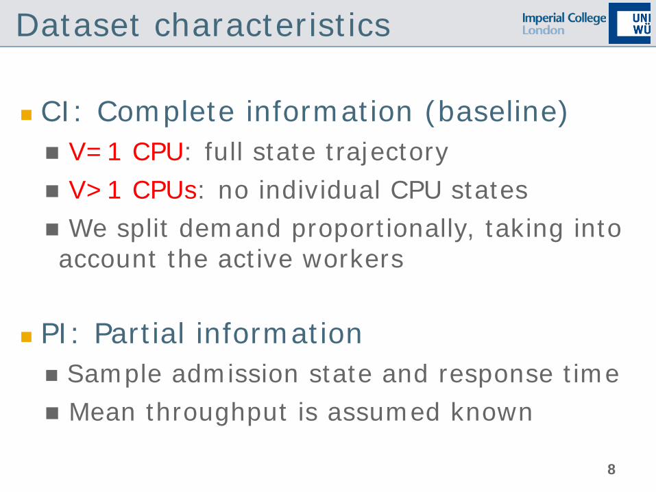
Dataset characteristics
CI: Complete information (baseline) V=1 CPU: full state trajectory V>1 CPUs: no individual CPU states We split demand proportionally, taking into account the active workers
PI: Partial information Sample admission state and response time Mean throughput is assumed known

9
CI: Demand estimation V=1 CPU Full demand distribution
Request Runtime
Active workers
Demand Request j
Class r
Scale by Active CPUs V>1 CPU
10
0
1
2
3
4
5
6
7
8
9
10
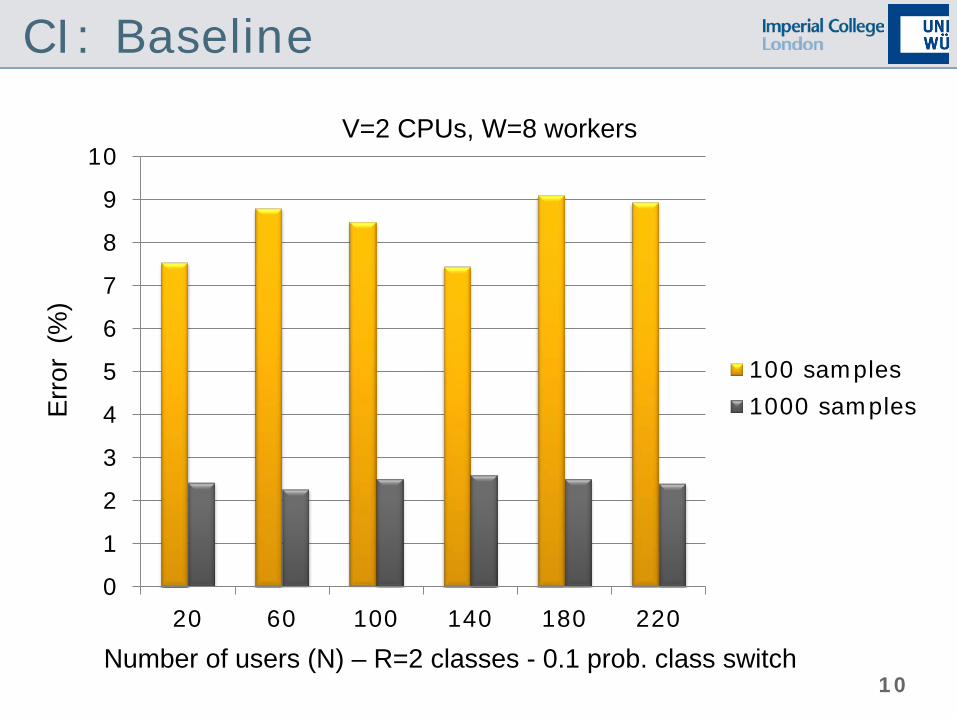
20 60 100 140 180 220
100 samples1000 samples
CI: Baseline
Number of users (N) – R=2 classes - 0.1 prob. class switch
Err
or (
%)
V=2 CPUs, W=8 workers

11
CI requires very detailed measurements Closed queueing network model Assume a fixed mix as seen upon job arrival No class switching ( tractable) Model can estimate response time of arriving job
PI: Approximation
CPU-0
CPU-1
Admission
Inter Admission
Time
CPU 0+1 (PS queue)
12
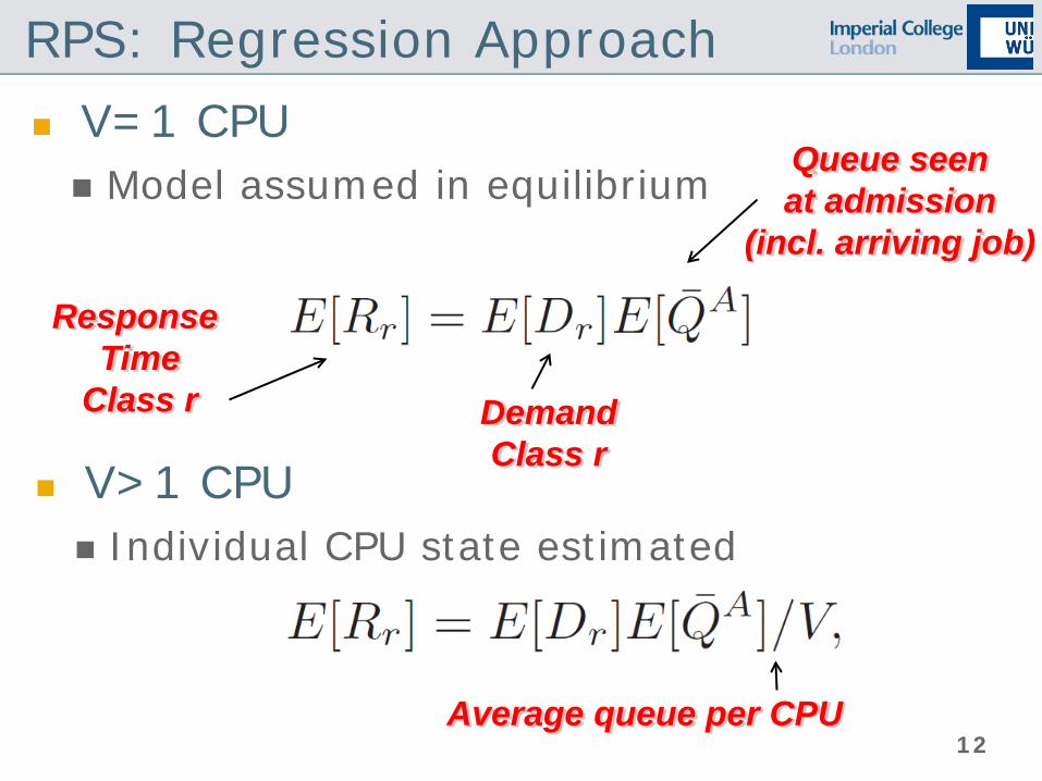
V=1 CPU Model assumed in equilibrium
RPS: Regression Approach
Queue seen at admission
(incl. arriving job)
Response Time
Class r
V>1 CPU Individual CPU state estimated
Demand Class r
Average queue per CPU
13
0.00
20.00
40.00
60.00
80.00
100.00
120.00
140.00
160.00
20 60 100 140 180 220
CIRPS
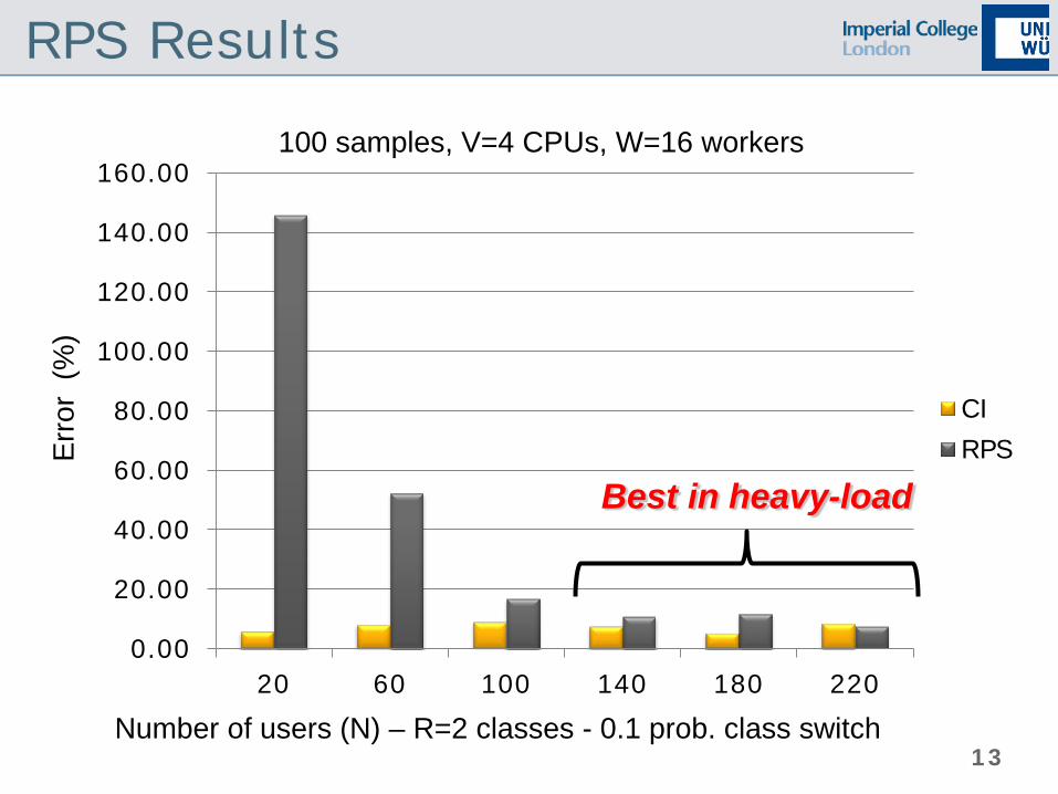
RPS Results
100 samples, V=4 CPUs, W=16 workers
Number of users (N) – R=2 classes - 0.1 prob. class switch
Err
or (
%)
Best in heavy-load

14
MLPS: Maximum Likelihood Maximum Likelihood Estimation (MLPS) Search over mean demand guesses Maximize likelihood of observed dataset
Response time likelihood Tagged customer method (absorbing CTMC) Initialized with state seen upon admission Mean demand guess CTMC rates

15
Job of class 3 arrives at system with V=1 CPU
Mix seen upon arrival: 1 job of class 1, 3 jobs of class 2
We study the transient of this CTMC to obtain the response time distribution of the class-3 job
MLPS: Absorbing CTMC
0,0,1
1,0,1
0,1,1
0,2,1
0,2,1
1,1,1
0,3,1
1,2,1
1,3,1
1/E[D3]
1/(2E[D3])
1/(3E[D3])
1/(4E[D3])
1/(5E[D3])
1/(4E[D3])
1/(3E[D3])
1/(2E[D3])
1/(3E[D3]) Initial state
Transitions depend on E[D1] and E[D2]

16
MLPS: Absorbing CTMC
V=1 CPU Dataset: Likelihood function for each sample:
V>1 CPUs Load-dependent rates
init with state at admission
trajectory in ri sec
completion rates
CTMC generator
1/demand

17
0.00
5.00
10.00
15.00
20.00
25.00
30.00
35.00
20 60 100 140 180 220
CIMLPS
MLPS: Results
Number of users (N) – R=2 classes - 0.1 prob. class switch
Err
or (
%)
100 samples, V=4 CPUs, W=16 workers
Best in light load

18
0.00
2.00
4.00
6.00
8.00
10.00
12.00
20 60 100 140 180 220
CIMINPS
MinPS: min(DRPS, DMLPS)
100 samples, V=4 CPUs, W=16 workers
Number of users (N) – R=2 classes - 0.1 prob. class switch
Err
or (
%)
best in light or heavy load

19
1
10
100
1,000
2 4 8 16 32 64
MLPSFMLPSRPS/ERPS
MinPS: ODE Approximation
100 samples: W=128 workers
V (CPUs)
Run
ning
Tim
e [s
]
exponential growth
scalable ODE approx

20
MinPS: Sensitivity Analysis
Magnitude of class demands 3 orders of difference: CI gap ~insensitive
Class switch probability High / Rare: CI gap ~insensitive
Non-exponential service low CV: CI gap weakly sensitive high CV: CI gap ~insensitive for CV<2
21
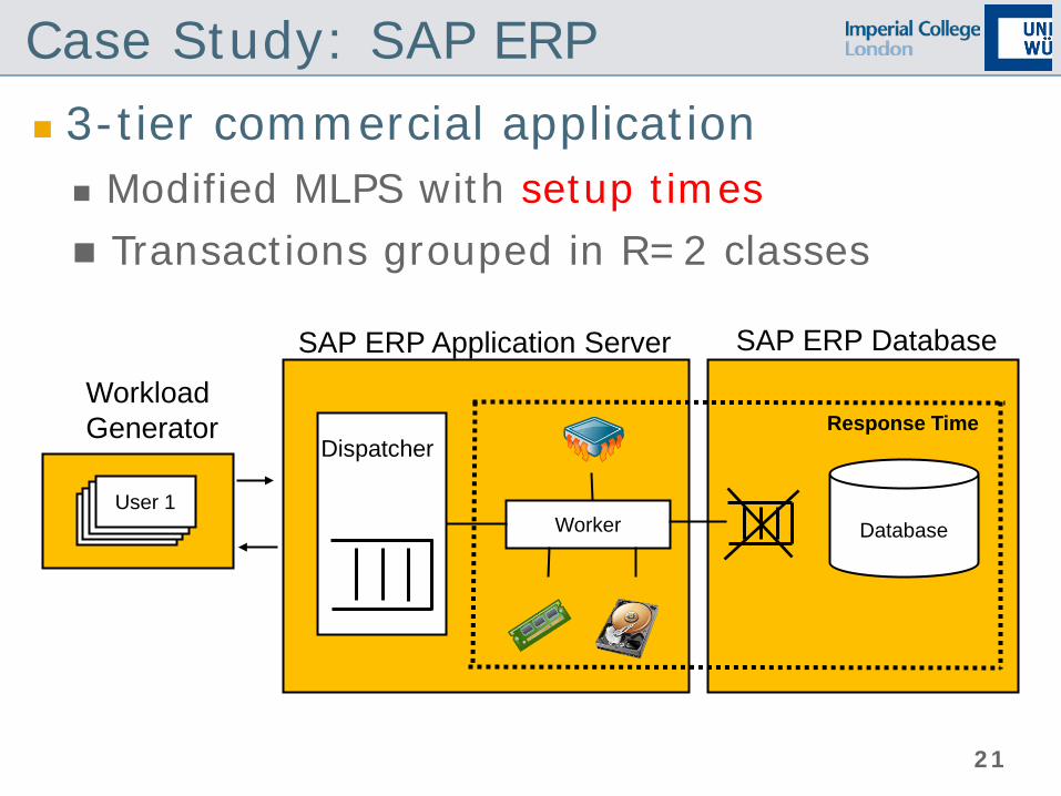
Case Study: SAP ERP 3-tier commercial application Modified MLPS with setup times Transactions grouped in R=2 classes
Response Time
User 1 Worker Database
SAP ERP Application Server
Workload Generator
Dispatcher
SAP ERP Database

22
0
0.05
0.1
0.15
0.2
0.25
N 5N 7N 10N 15N
MEASSIM
SAP ERP Queueing Model
Measured vs Simulation with Estimated Demands
Population - Baseline N = [6 jobs class 1, 4 jobs class 2]
Res
pons
e T
ime
23
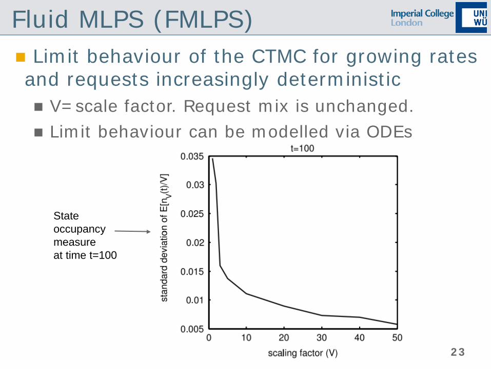
Fluid MLPS (FMLPS) Limit behaviour of the CTMC for growing rates and requests increasingly deterministic V=scale factor. Request mix is unchanged. Limit behaviour can be modelled via ODEs
State occupancy measure at time t=100

24
1
10
100
1,000
2 4 8 16 32 64
MLPSERPSFMLPS
Computational Costs
100 samples: W=128 workers
V (CPUs)
Run
ning
Tim
e [s
]
CTMC: exponential complexity
Fluid: scalable
(RPS, <1s)
25
0
2
4
6
8
10
12
20 60 100 140 180
CIFMLPS
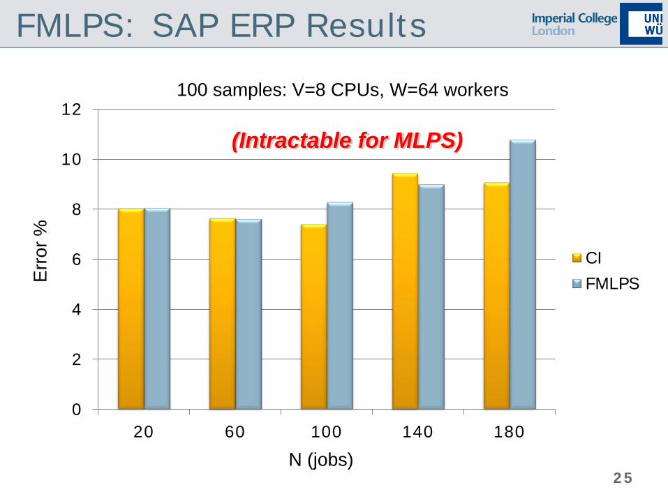
FMLPS: SAP ERP Results
100 samples: V=8 CPUs, W=64 workers
N (jobs)
Err
or %
(Intractable for MLPS)

26
Queue-Length Based Estimation

27
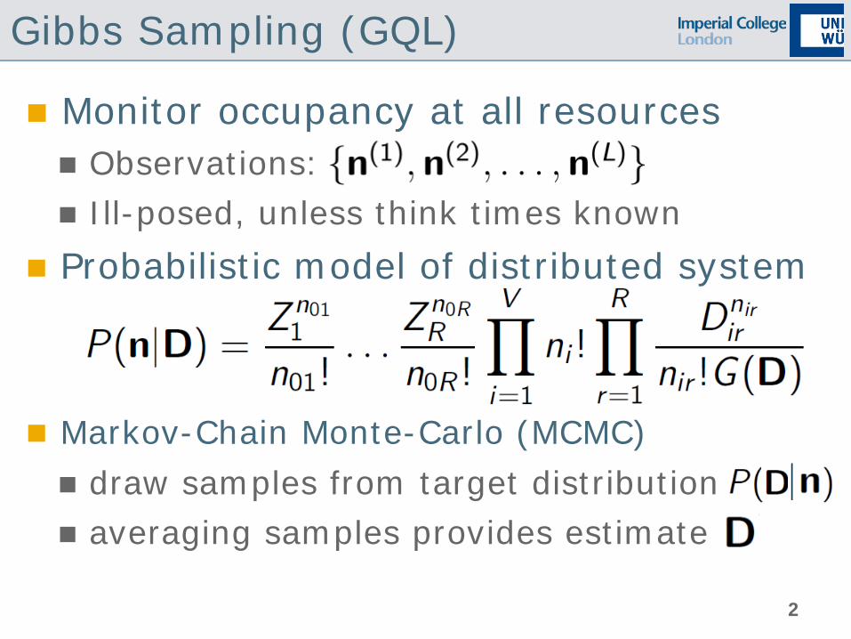
Monitor occupancy at all resources Observations: Ill-posed, unless think times known
Probabilistic model of distributed system
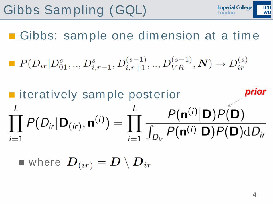
Gibbs: iteratively sample posterior
Gibbs Sampling (GQL)
prior

28
GQL: Results
Accurate estimates, error ~3%-7%

29
GQL: Sensitivity analysis Increasing model sizes
05
101520253035404550
4 6 8 13 20 28 89 127 186
GQL
GQLErr
or (%
)
Log of state space size

30
GQL: Prior distribution
Dirichlet prior all estimates converge unless the exact demand has very low probability prior

31
GQL: Results
Accurate estimates, error ~3%-7%

32
GQL vs Other MCMC Methods
Far better convergence properties than Metropolis-Hastings and Slice sampling About 13-15% error in estimating demands against cloud ERP data (Apache OFBiz)

33
QMLE Approximation
Based on Maximum Likelihood Estimation
Works with mean queue length
A simple approximation of the MLE:
Consider the demand vector where
More details at tomorrow’s talk!

34
FG Tool
35
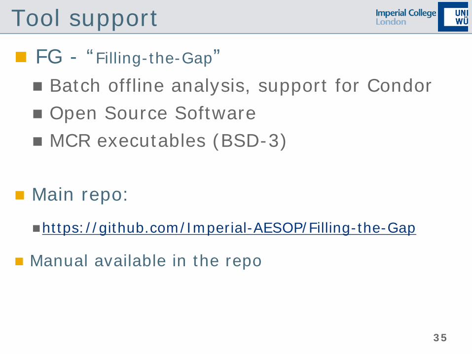
Tool support FG - “Filling-the-Gap” Batch offline analysis, support for Condor Open Source Software MCR executables (BSD-3)
Main repo:
https://github.com/Imperial-AESOP/Filling-the-Gap
Manual available in the repo

36
FG: Initial design Outputs Model parameters Visualization Forecasting
–Requires analysis, but not decision-making User control knobs Analysis frequency Horizon of analysis Monitoring intensity Maximum collection window

37
FG: Parameter Estimation
Parameters for QN/LQN models

38
FG: Architecture

39
FG: Methods Implemented methods Complete Information (CI) Utilization-Based Regression (UBR) Utilization-Based Optimization (UBO) (M/GI/1-PS; cf. Zhang et al., Menasce) ODE-based MLPS (“fluid MLPS”, FMLPS) MINPS Queue-Based Gibbs Sampling (GQL) Extended RPS (ERPS, includes a new correction for number of cores)

40
FG: Comparison Results

1
Queue-Length Based Estimation
2
Monitor occupancy at all resources Observations: Ill-posed, unless think times known
Probabilistic model of distributed system
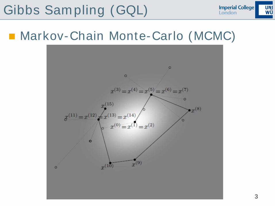
Markov-Chain Monte-Carlo (MCMC) draw samples from target distribution averaging samples provides estimate
Gibbs Sampling (GQL)
3
Markov-Chain Monte-Carlo (MCMC)
Gibbs Sampling (GQL)
4
Gibbs: sample one dimension at a time
iteratively sample posterior
where
Gibbs Sampling (GQL)
prior

5
GQL: Results
Accurate estimates, error ~3%-7%

6
GQL: Sensitivity analysis Increasing model sizes
05
101520253035404550
4 6 8 13 20 28 89 127 186
GQL
GQLErr
or (%
)
Log of state space size

7
GQL: Prior distribution
Dirichlet prior all estimates converge unless the exact demand has very low probability prior

8
GQL: Results
Accurate estimates, error ~3%-7%

9
GQL vs Other MCMC Methods
Far better convergence properties than Metropolis-Hastings and Slice sampling About 13-15% error in estimating demands against cloud ERP data (Apache OFBiz)

10
QMLE Approximation
Based on Maximum Likelihood Estimation
Works with mean queue length
A simple approximation of the MLE:
Consider the demand vector where
Approach generalizes to load-dependent QNs
More details at tomorrow’s talk!

11
FG Tool

12
Tool support FG - “Filling-the-Gap” Batch offline analysis, support for Condor Open Source Software MCR executables (BSD-3)
Main repo:
https://github.com/Imperial-AESOP/Filling-the-Gap
Manual available in the repo
13
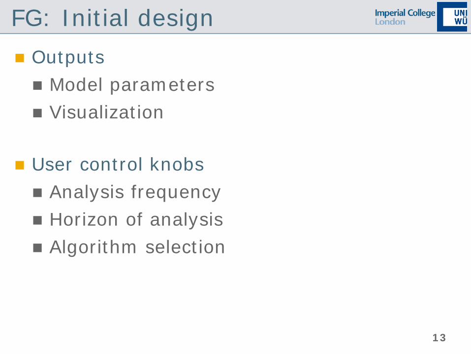
FG: Initial design Outputs Model parameters Visualization
User control knobs Analysis frequency Horizon of analysis Algorithm selection

14
FG: Parameter Estimation
Parameters for QN/LQN models

15
FG: Architecture

16
FG: Methods Implemented methods Complete Information (CI) Utilization-Based Regression (UBR) Utilization-Based Optimization (UBO) (M/GI/1-PS; cf. Zhang et al., Menasce) ODE-based MLPS (“fluid MLPS”, FMLPS) MINPS Queue-Based Gibbs Sampling (GQL) Extended RPS (ERPS, includes a new correction for number of cores)

17
FG: Comparison Results

1
Comparison & Case Studies

2
Comparison
Elsevier PEVA, October 2015.

3
Experiments Dataset D1: Queueing Simulator Simulated M/M/1 queue with FCFS scheduling Workload classes: 1, 2 and 5 Utilization levels: 10%, 50%, 90% In total: 900 traces
Dataset D2: Micro-Benchmarks Workload classes: 1, 2, and 3 Utilization levels: 20%, 50%, 80% In total: 210 traces

4
Compared Approaches Based on Service Demand Law (Brosig et al. 2009) Utilization Regression (Rolia and Vetland 1995) Kalman Filter (Kumar et al. 2009) Opitimization 1 (Menascé 2008) Optimization 2 (Liu et al. 2006) Response time regression (Kraft et al. 2009) Gibbs Sampling (Wang et al. 20133)

5
Sampling Interval
0
20
40
60
80
100
120
Util. Regression Kalman Filter Optim. 1 Optim. 2
Rela
tive
Erro
r (i
n %
)
1 s 5 s 10 s 30 s 60 s 120 s
Number of requests within one interval should be larger than 60.
Dataset D1

6
Number of Samples
0
1
2
3
4
5
6
7
8
SDL Util.Regression
Kalman Filter Optim. 1 Optim. 2 Rt. Regression Gibbs
Rela
tive
Erro
r (i
n %
)
600 samples 3600 samples
Dataset D1
Number of samples has only limited impact.

7
Number of Workload Classes
0
20
40
60
80
100
120
140
160
180
SDL Util.Regression
Kalman Filter Optim. 1 Optim. 2 Rt.Regression
Gibbs
Rela
tive
Erro
r (i
n %
)
1 class 2 classes 5 classes
Dataset D1
Number of classes has strong impact on D1.

8
Number of workload classes
0
5
10
15
20
25
30
SDL Util.Regression
Kalman Filter Optim. 1 Optim. 2 Rt. Regression Gibbs
Rela
tive
Erro
r (i
n %
)
1 class 2 classes 3 classes
Dataset D2
Number of classes has a much smaller impact on D2.

9
Correlation Analysis C
lass
es
SD
L
Uti
l.
Reg
ress
ion
Kal
man
Filt
er
Op
tim
. 1
Op
tim
. 2
Rt.
Reg
ress
ion
Gib
bs
2 0.91 0.35 0.88 0.89 0.88 0.52 0.9 5 0.72 0.37 0.78 0.8 0.8 0.44 0.79
Correlation with std[D]:
Significant influence of scheduling strategy.

10
Load Level
0
10
20
30
40
50
60
70
80
90
100
SDL Util.Regression
Kalman Filter Optim. 1 Optim. 2 Rt.Regression
Gibbs
Rela
tive
Erro
r (i
n %
)
10% 50% 90%
Dataset D1
High utilization observations can impact estimation negatively.

11
Collinearity
0
20
40
60
80
100
120
SDL Util.Regression
Kalman Filter Optim. 1 Optim. 2 Rt.Regression
Gibbs
Rela
tive
Erro
r (i
n %
)
Low High
Collinearity in throughputs impacts Utilization Regression

12
Missing Jobs
0
10
20
30
40
50
60
70
80
90
100
SDL Util.Regression
Kalman Filter Optim. 1 Optim. 2 Rt.Regression
Gibbs
Rela
tive
Erro
r (i
n %
)
5% 10% 20% 30%
Higher influence on utilization approaches than on response time ones.
13
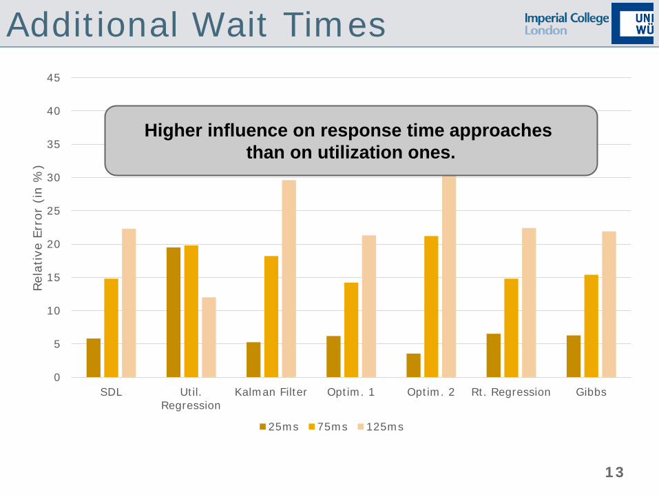
Additional Wait Times
0
5
10
15
20
25
30
35
40
45
SDL Util.Regression
Kalman Filter Optim. 1 Optim. 2 Rt. Regression Gibbs
Rela
tive
Erro
r (i
n %
)
25ms 75ms 125ms
Higher influence on response time approaches than on utilization ones.

14
Execution Time
0.10
1.00
10.00
100.00
1000.00
10000.00
100000.00
1000000.00
SDL Util.Regression
KalmanFilter
Optim. 1 Optim. 2 Rt.Regression
Gibbs
Exec
utio
n Ti
me
(in
ms)
1 class 2 classes 5 classes

15
Case Study: SPECjEnterprise SPECjEnterprise2010 application benchmark Distributed deployment over 7 VMs „Microservice Style“
Strategies for Demand Estimation Observed end-to-end response time Observed residence time per tier Per-resource statistics

16
Experiment Setup

17
Results
0
10
20
30
40
50
60
70
80
90
100
Purchase Manage Browse Mfg EJB Mfg WS
Rela
tive
Erro
r (%
)
Prediction Error Response Time
Optim. 2 (System) Optim. 2 (Tier) SDL
18
Results
0
10
20
30
40
50
60
70
80
90
100
VM 2 VM 3 VM 4 VM 5 VM 6 VM 7 VM 9
Rela
tive
Erro
r (%
)
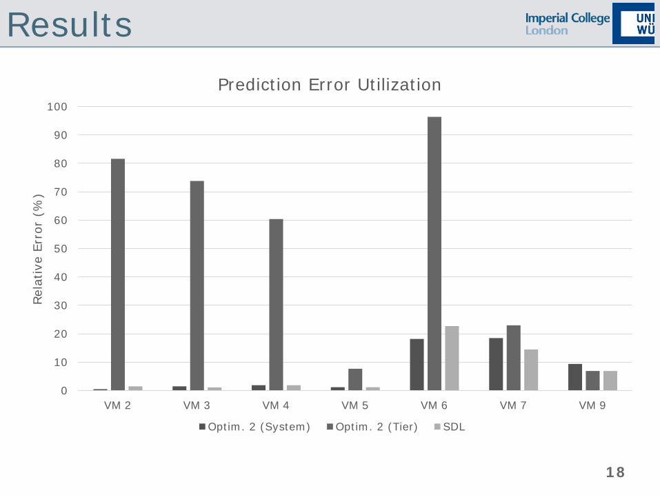
Prediction Error Utilization
Optim. 2 (System) Optim. 2 (Tier) SDL

19
Case Study: SAP HANA Admission control Multi-tenant application (extended TPC-W) SAP HANA cloud platform
Supports Performance isolation between tenants IEEE/ACM CCGrid 2014.

20
General Idea
Application Server
Admission Control
Requests rr,c
Tenants
Accepted Request
Response
Resource Demand Estimation
Demand dt,r,i
Guarantee
Indices:
t = tenant
r = request type
i = resource
Moni-toring
Throughput Xt,r Response Time Rt,r
Utilization Ui

21
Resource Isolation

22
Performance Isolation

23
Case Study: Zimbra Goal: Automatic vertical CPU scaling of VMs Zimbra is a collaboration server Transactional workload SLA: Mails need to be delivered within 2 minutes Mails may be queued
IEEE SASO 2014.

24
Approach Overview
Desired resource allocation (at+1)
VM1
VM2
VMn
... Applicatio
n Controller
Model Builder
Model: p = f(λ,a)
Current resource usage (ut)
App-level SLO (pref)
App Sensor
System Sensor
Observed app performance (pt)
pt
vApp Manager
New VM resource settings (number of vCPUs, configured memory size)
vApp

25
Layered Performance Model
Application layer
Virtual resource layer
Physical resource layer
VM1 VM2 vApp
vCPU vCPU
Physical CPU Service rate depends on physical hardware
+ Hypervisor Scheduling Delays
+ OS scheduling delays + Wait times for other
resources
Hierarchical modeling approach (Method of Layers [1]): Service time at layer 𝑖𝑖 is equal to response time of an underlying closed queueing network at layer 𝑖𝑖 − 1
Load-dependent Service Demands

26
Influence of Layers
Zimbra MTA with linearly increasing workload:
Dem
ands
(in
seco
nds)
Estimated demands reflect contention at hypervisor and application level
27
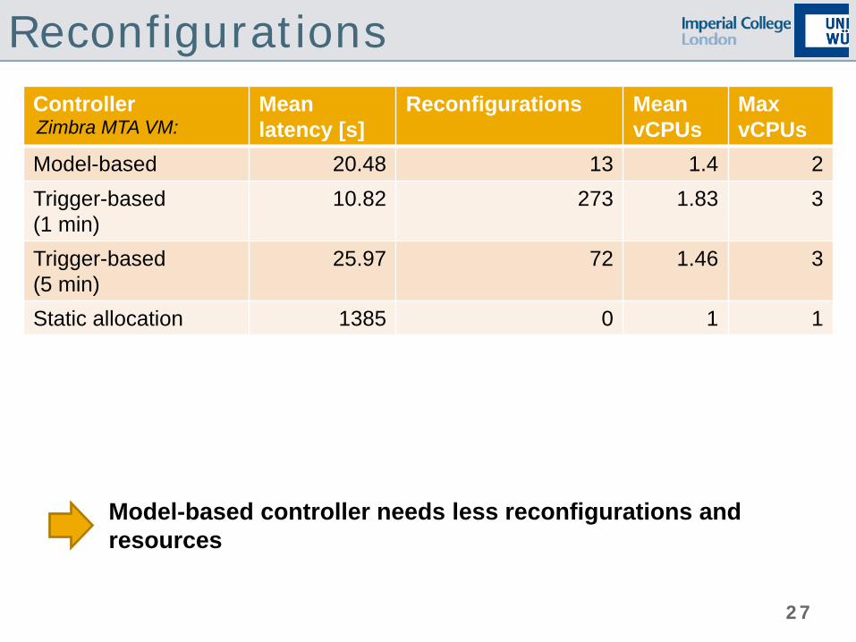
Reconfigurations Controller Mean
latency [s] Reconfigurations Mean
vCPUs Max vCPUs
Model-based 20.48 13 1.4 2 Trigger-based (1 min)
10.82 273 1.83 3
Trigger-based (5 min)
25.97 72 1.46 3
Static allocation 1385 0 1 1
Zimbra MTA VM:
Model-based controller needs less reconfigurations and resources
28
Bibliography Menascé, D. A. (2008). “Computing missing service demand parameters for performance models”. In: CMG Conference Proceedings, pp. 241–248
Liu, Z., L. Wynter, C. H. Xia, and F. Zhang (2006). “Parameter inference of queueing models for IT systems using end-to-end measurements”. In: Perform. Eval. 63.1, pp. 36–60
Kumar, D., A. N. Tantawi, and L. Zhang (2009a). “Real-time performance modeling for adaptive software systems with multi-class workload”. In: Proceedings of the 17th Annual Meeting of the IEEE/ACM International Symposium on Modelling, Analysis and Simulation of Computer and Telecommunication Systems, MASCOTS, pp. 1–4
Zheng, T., C. M. Woodside, and M. Litoiu (2008). “Performance Model Estimation and Tracking Using Optimal Filters”. In: IEEE Trans. Software Eng. 34.3, pp. 391–406

29
Bibliography Wang, W., X. Huang, X. Qin, W. Zhang, J. Wei, and H. Zhong (2012). “Application-Level CPU Consumption Estimation: Towards Performance Isolation of Multi-tenancy Web Applications”. In: Proceedings of the 2012 IEEE Fifth International Conference on Cloud Computing, CLOUD, pp. 439–446
Brosig, F., S. Kounev, and K. Krogmann (2009). “Automated extraction of palladio component models from running enterprise Java applications”. In: Proceedings of the 4th International Conference on Performance Evaluation Methodologies and Tools, VALUETOOLS, p. 10
Rolia, J. and V. Vetland (1995). “Parameter estimation for performance models of distributed application systems”. In: Proceedings of the 1995 Conference of the Centre for Advanced Studies on Collaborative Research, CASCON, p. 54

30
Bibliography Kraft, S., S. Pacheco-Sanchez, G. Casale, and S. Dawson (2009). “Estimating service resource consumption from response time measurements”. In: Proceedings of the 4th International Conference on Performance Evaluation Methodologies and Tools, VALUETOOLS, p. 48 Wang, W. and G. Casale (2013). “Bayesian Service Demand Estimation Using Gibbs Sampling”. In: Proceedings of the 2013 IEEE 21st International Symposium on Modelling, Analysis and Simulation of Computer and Telecommunication Systems, MASCOTS, pp. 567–576 G. Casale, P. Cremonesi, R. Turrin, Robust Workload Estimation in Queueing Network Performance Models, in: 16th Euromicro Conference on Parallel, Distributed and Network-Based Processing (PDP), 2008, pp. 183-187.

31
Bibliography P. Cremonesi, K. Dhyani, A. Sansottera, Service Time Estimation with a Refinement Enhanced Hybrid Clustering Algorithm, in: Analytical and Stochastic Modeling Techniques and Applications, Vol. 6148 of Lecture Notes in Computer Science, Springer Berlin / Heidelberg, 2010, pp. 291--305 P. Cremonesi, A. Sansottera, Indirect estimation of service demands in the presence of structural changes, Performance Evaluation 73 (0) (2014) 18--40, special Issue on the 9th International Conference on Quantitative Evaluation of Systems

1
Arrival Process Fitting
Joint work with A. Sansottera and P. Cremonesi (DEIB, Politecnico di Milano, Italy)

2
Outline Introduction
Moments and probabilities in Marked MAPs
Fitting of second-order acyclic Marked MAPs
Results
Conclusions

3
Requests Traffic
Time-Varying Peaks of User Activity
High Performance
Will the system sustain the load?
Sun Mon Tue Wed Thu
request number
Inter-arrival times
[µs]
FAST RATE
SLOW RATE
SLOW RATE
FAST RATE
SLOW RATE

4
Stochastic models Generate statistically similar request arrival patterns Analytical models accelerate search for optimal decisions
Markovian Traffic Model
request number
Inter-arrival times
[µs]
Arrival Process Modelling
Stochastic analysis
SLOW RATE
FAST RATE
FAST RATE
SLOW RATE
30%
70%
50%
50%
Request number
Inte
rarr
ival
tim
e [m
s]
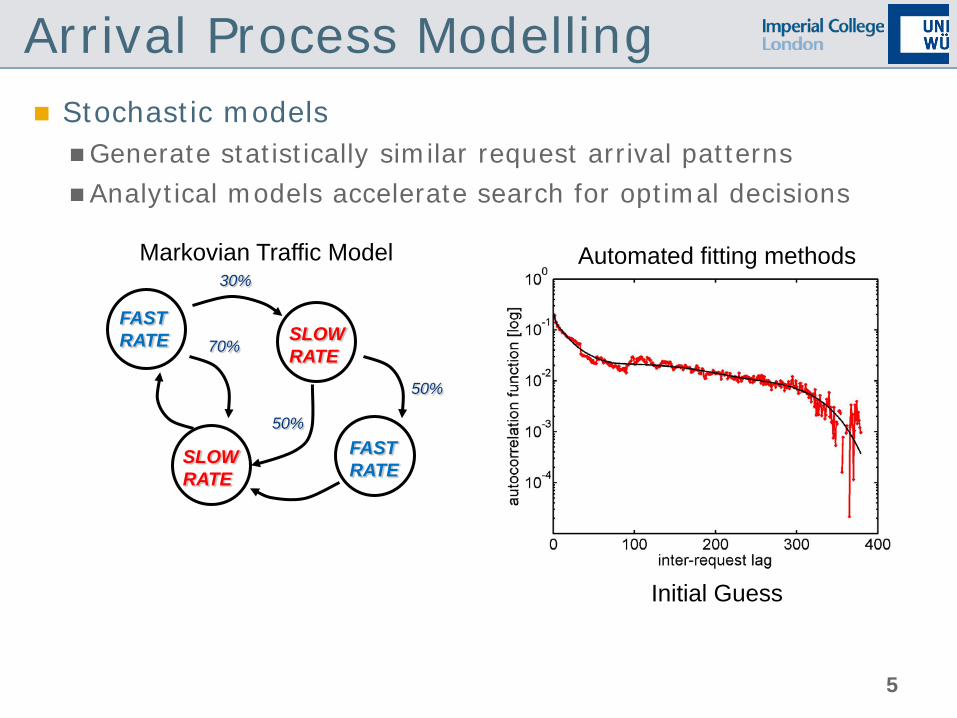
5
Stochastic models Generate statistically similar request arrival patterns Analytical models accelerate search for optimal decisions
Arrival Process Modelling
SLOW RATE
FAST RATE
FAST RATE
SLOW RATE
Markovian Traffic Model Automated fitting methods 30%
70%
50%
50%
Models evaluated: ~350 Initial Guess

6
Network of queues mathematical abstraction for prediction, what-if scenarios, … describes billions of possible states for the resources efficient output analysis techniques [Smirni, QEST’09]
Incoming Requests
Traffic Decomposition for QN
FAST RATE
SLOW RATE
Completed Requests
Web Server
Storage
Database
CPU
Disks
CPUs
Cloud Resources

7
Network of queues mathematical abstraction for prediction, what-if scenarios, … describes billions of possible states for the resources developed efficient analysis techniques
Output Flow
Traffic Decomposition for QN
Completed Requests
Storage
Database
Disks
CPUs
FAST RATE
SLOW RATE
SLOW RATE
Cloud Resources

8
Network of queues mathematical abstraction for prediction, what-if scenarios, … describes billions of possible states for the resources developed efficient analysis techniques
Output Flow
Traffic Decomposition for QN
Completed Requests
Storage
Database
Disks
CPUs
FAST RATE
SLOW RATE
SLOW RATE
Cloud Resources
9
Network of queues mathematical abstraction for prediction, what-if scenarios, … describes billions of possible states for the resources developed efficient analysis techniques
Output Flow
Traffic Decomposition for QN
Completed Requests
SLOW RATE
FAST RATE
SLOW RATE
FAST RATE
Cloud Resources

10
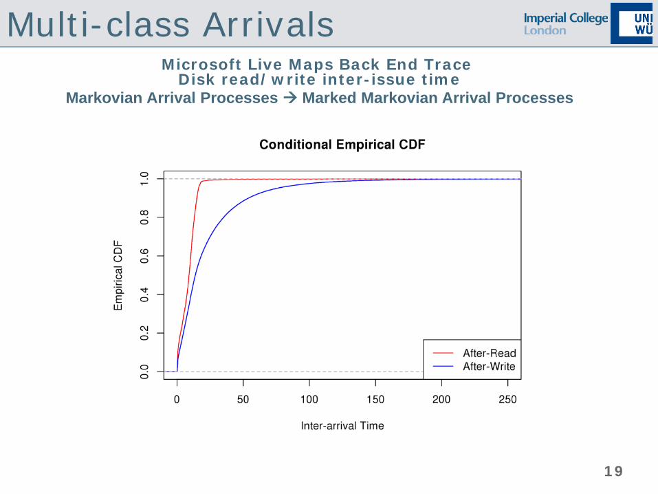
Non-Poisson Arrivals Microsoft Live Maps Back End Trace
Disk read/write inter-issue time Poisson Phase-type Renewal Processes

11
PH-type Distribution N transient states
Exit vector
No-mass at 0 assumption
CTMC
Representation PH(D0, α)
1 absorbing state
Phase-type Distribution: distribution of the time to absorption
12
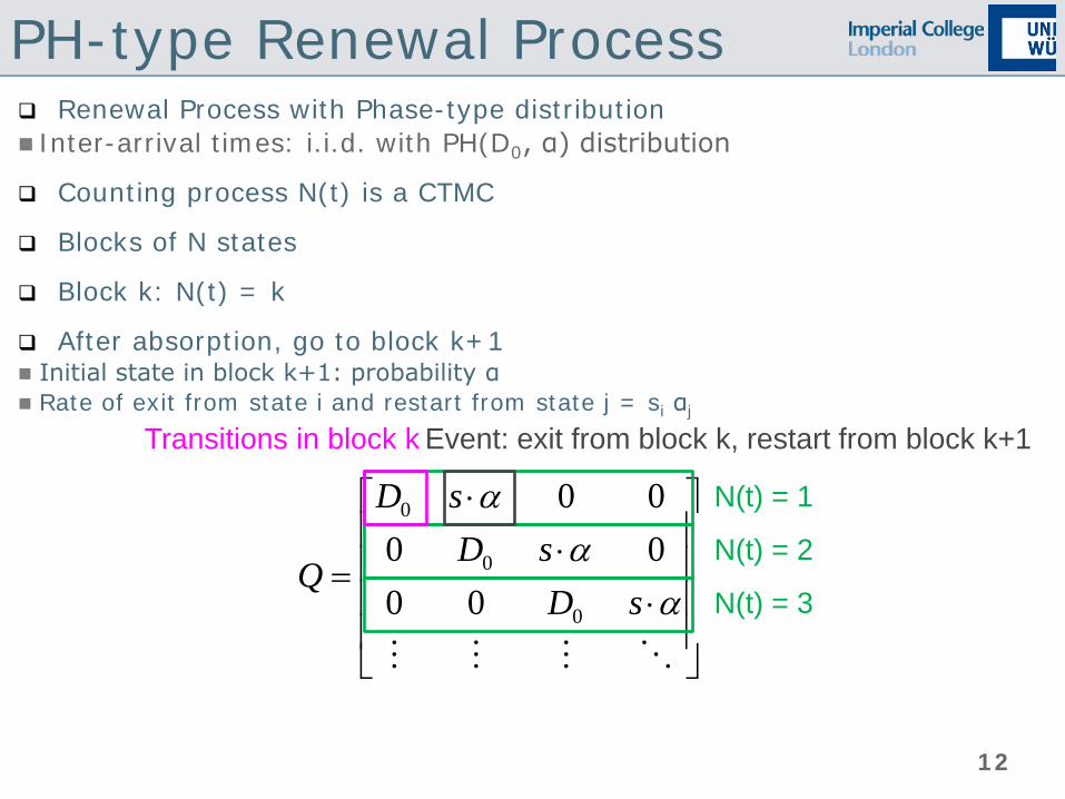
PH-type Renewal Process Renewal Process with Phase-type distribution Inter-arrival times: i.i.d. with PH(D0, α) distribution
Counting process N(t) is a CTMC
Blocks of N states
Block k: N(t) = k
After absorption, go to block k+1 Initial state in block k+1: probability α Rate of exit from state i and restart from state j = si αj
⋅⋅
⋅
=
αα
α
sDsD
sD
Q0
0
0
000000
Transitions in block k
N(t) = 2
N(t) = 3
Event: exit from block k, restart from block k+1
N(t) = 1

13
Some Tools for PH Fitting
EMpht (1996) http://home.imf.au.dk/asmus/pspapers.html EM algorithm for ML fitting, based on Runge-Kutta methods Local optimization technique
jPhase (2006) http://copa.uniandes.edu.co/software/jmarkov/index.html
Java library ML and canonical form fitting algorithms

14
Some Tools for PH Fitting
PhFit (2002) http://webspn.hit.bme.hu/∼telek/tools.htm
Separate fit of distribution body and tail Both continuous and discrete ML distributions
G-FIT (2007) http://ls4-www.cs.uni-dortmund.de/home/thummler/gfit.tgz
Hyper-Erlang PHs used as building block Automatic aggregation of large traces, dramatic speed-up of computational times compared to EMpht

15
Correlated Arrivals Microsoft Live Maps Back End Trace
Disk read/write inter-issue time Phase-type Renewal Processes Markovian Arrival Processes

16
Markovian Arrival Process Phase-type Renewal Process Rate of exit from state i and restart from state j = si αj
Markovian Arrival Process (MAP) Rate of exit from state i and restart from state j = sij Generalization of PH-Renewal: allows to model correlation
=
10
10
10
000000
DDDD
DD
Q
−
−−
=
nnn rr
rrrr
D
λ
λλ
21
23221
13121
0
−
=
nnnn sss
ssssss
D
21
232221
131211
1Representation: MAP(D0,D1)
Interval-stationary initialization

17
Tools for MAP fitting
KPC-Toolbox (2008) http://www.cs.wm.edu/MAPQN/kpctoolbox.html Moment-matching method Composition of large MAPs by two-state MAPs Property of KPC Process (similar relations for higher-order moments, ACF, …)
KPC Process
!/][][][ kXEXEXE kb
ka
k =
18
Motivation and Goals Marked Markovian Arrival Processes (MMAPs) Generalization of MAPs to model multi-class arrivals Allow to model non-Poisson cross-correlated arrivals Allow efficient solution of the models with matrix-
analytic methods
Modeling the arrival process at a queuing system (MMAP[K]/PH[k]/1-FCFS queue) FCFS queues can be analyzed analytically using age process Q-MAM: https://bitbucket.org/qmam/qmam/src BU-Tools: http://webspn.hit.bme.hu/~telek/tools/butools/
19
Multi-class Arrivals Microsoft Live Maps Back End Trace
Disk read/write inter-issue time Markovian Arrival Processes Marked Markovian Arrival Processes

20
Marked MAPs
(D0,D1) is a representation of the MAP underlying the MMAP
(D0,D11,D12) is a representation of a MMAP[2] process (2 classes)

21
Fitting Fitting problem Marked trace from a real system: (Xi, Ci) MMAP Queues with arrivals that follow MMAP can be solved
analytically
Two families of methods Maximum-likelihood Matching moments (or other characteristics)
We focus on moment matching More computationally efficient In real systems, easier to save moments than the whole
trace

22
Issues of moment matching Representation of MMAPs is not minimal Number of parameters >> Degrees of freedom
Hard to obtain analytical fitting formulas for the parameters Easy: Parameters -> Moments Hard: Moments -> Parameters Requires solving a non-linear system of equations in the
general case Non-linear least squares for MMAP fitting [Buchholz, 2010]
23
Issues of moment matching Feasibility: given a number of states n for the
MMAP, which values of the moments can be fitted exactly? Related issue: how to perform approximate fitting?
Which characteristics best capture the queueing behavior? Caveat 1: not all characteristics have known analytical
formulas Caveat 2: inverting the analytical formulas might be harder
for some characteristics

24
Outline Introduction
Moments and probabilities in Marked MAPs
Fitting of second-order acyclic Marked MAPs
Results

25
Definitions Ordinary moment of order j:
Backward moment of order j for class c (green):
Forward moment of order j for class c (green):
Cross moments of order j for class c followed by class k:
Probability of a class c arrival:
“Transition” probability of a class c arrival followed by class k
26
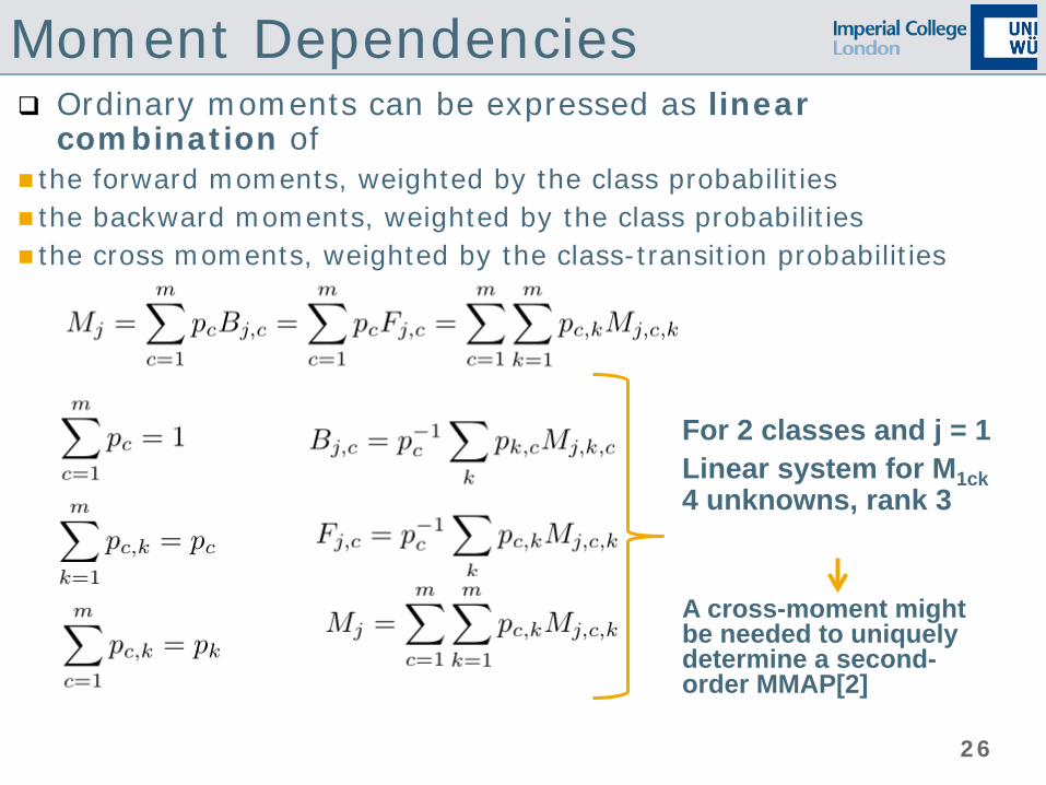
Moment Dependencies Ordinary moments can be expressed as linear
combination of the forward moments, weighted by the class probabilities the backward moments, weighted by the class probabilities the cross moments, weighted by the class-transition probabilities
For 2 classes and j = 1 Linear system for M1ck 4 unknowns, rank 3
A cross-moment might be needed to uniquely determine a second-order MMAP[2]

27
Outline Introduction
Moments and probabilities in Marked MAPs
Fitting of second-order acyclic Marked MAPs
Results

28
AMMAP[2] Fitting
7 degrees of freedom
4 for the underlying
AMAP
3 for the marginal
Phase-type
1 for the auto-
correlation decay
3 for multi-class
characteristics
D0 D1

29
AMMAP[2] Fitting Any MAP(2) has geometric autocorrelation decay with rate γ • Canonical form for the underlying MAP(2) [Bodrog et al., 2010] Acyclic: two forms for γ > 0 and γ < 0 For γ = 0, acyclic phase-type renewal
γ > 0 γ < 0

30
AMMAP[2] Fitting Any MAP(2) has geometric autocorrelation decay with rate γ • Canonical form for the underlying MAP(2) [Bodrog et al., 2010] Acyclic: two forms for γ > 0 and γ < 0 For γ = 0, acyclic phase-type renewal
γ > 0 γ < 0
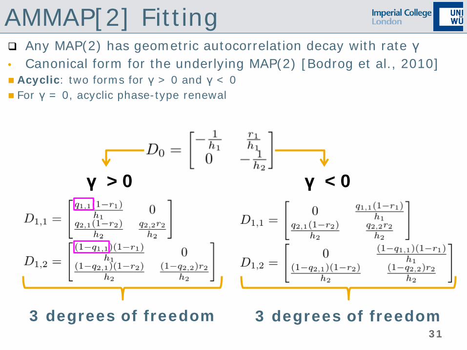
31
AMMAP[2] Fitting Any MAP(2) has geometric autocorrelation decay with rate γ • Canonical form for the underlying MAP(2) [Bodrog et al., 2010] Acyclic: two forms for γ > 0 and γ < 0 For γ = 0, acyclic phase-type renewal
γ > 0 γ < 0
3 degrees of freedom 3 degrees of freedom

32
AMMAP[2] Fitting How to spend the 3 available degrees of
freedom?
We have found closed, analytical formulas for the three parameters q11, q21, q22, for both canonical forms
Three different sets of characteristics considered Class probabilities and… 1) Forward moments and backward moments 2) Forward moments and class transition probabilities 3) Backward moments and class transition probabilities
33
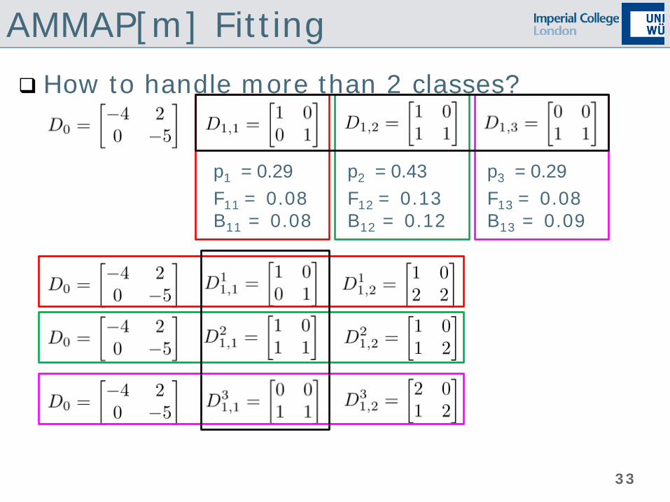
AMMAP[m] Fitting How to handle more than 2 classes?
p1 = 0.29 F11 = 0.08 B11 = 0.08
p2 = 0.43 F12 = 0.13 B12 = 0.12
p3 = 0.29 F13 = 0.08 B13 = 0.09
34
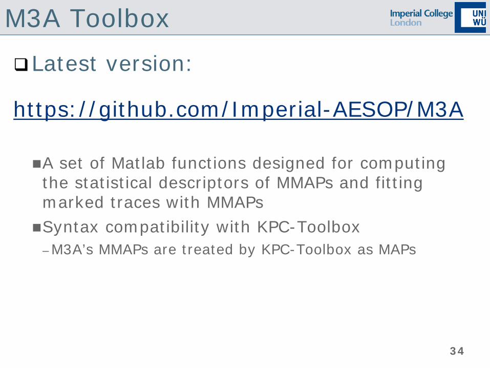
M3A Toolbox
Latest version:
https://github.com/Imperial-AESOP/M3A A set of Matlab functions designed for computing the statistical descriptors of MMAPs and fitting marked traces with MMAPs Syntax compatibility with KPC-Toolbox
– M3A’s MMAPs are treated by KPC-Toolbox as MAPs

35
Outline Introduction
Moments and probabilities in Marked MAPs
Fitting of second-order acyclic Marked MAPs
Results

36
Real-World Traces
Microsoft Live Maps Back End Trace – Disk read/write inter-issue time
Simulation of */M/1 Queue

37
Bibliography Menascé, D. A. (2008). “Computing missing service demand parameters for performance models”. In: CMG Conference Proceedings, pp. 241–248
Liu, Z., L. Wynter, C. H. Xia, and F. Zhang (2006). “Parameter inference of queueing models for IT systems using end-to-end measurements”. In: Perform. Eval. 63.1, pp. 36–60
Kumar, D., A. N. Tantawi, and L. Zhang (2009a). “Real-time performance modeling for adaptive software systems with multi-class workload”. In: Proceedings of the 17th Annual Meeting of the IEEE/ACM International Symposium on Modelling, Analysis and Simulation of Computer and Telecommunication Systems, MASCOTS, pp. 1–4
Zheng, T., C. M. Woodside, and M. Litoiu (2008). “Performance Model Estimation and Tracking Using Optimal Filters”. In: IEEE Trans. Software Eng. 34.3, pp. 391–406

38
Bibliography Wang, W., X. Huang, X. Qin, W. Zhang, J. Wei, and H. Zhong (2012). “Application-Level CPU Consumption Estimation: Towards Performance Isolation of Multi-tenancy Web Applications”. In: Proceedings of the 2012 IEEE Fifth International Conference on Cloud Computing, CLOUD, pp. 439–446
Brosig, F., S. Kounev, and K. Krogmann (2009). “Automated extraction of palladio component models from running enterprise Java applications”. In: Proceedings of the 4th International Conference on Performance Evaluation Methodologies and Tools, VALUETOOLS, p. 10
Rolia, J. and V. Vetland (1995). “Parameter estimation for performance models of distributed application systems”. In: Proceedings of the 1995 Conference of the Centre for Advanced Studies on Collaborative Research, CASCON, p. 54
39
Bibliography Kraft, S., S. Pacheco-Sanchez, G. Casale, and S. Dawson (2009). “Estimating service resource consumption from response time measurements”. In: Proceedings of the 4th International Conference on Performance Evaluation Methodologies and Tools, VALUETOOLS, p. 48 Wang, W. and G. Casale (2013). “Bayesian Service Demand Estimation Using Gibbs Sampling”. In: Proceedings of the 2013 IEEE 21st International Symposium on Modelling, Analysis and Simulation of Computer and Telecommunication Systems, MASCOTS, pp. 567–576 G. Casale, P. Cremonesi, R. Turrin, Robust Workload Estimation in Queueing Network Performance Models, in: 16th Euromicro Conference on Parallel, Distributed and Network-Based Processing (PDP), 2008, pp. 183-187.

40
Bibliography P. Cremonesi, K. Dhyani, A. Sansottera, Service Time Estimation with a Refinement Enhanced Hybrid Clustering Algorithm, in: Analytical and Stochastic Modeling Techniques and Applications, Vol. 6148 of Lecture Notes in Computer Science, Springer Berlin / Heidelberg, 2010, pp. 291--305
P. Cremonesi, A. Sansottera, Indirect estimation of service demands in the presence of structural changes, Performance Evaluation 73 (0) (2014) 18--40, special Issue on the 9th International Conference on Quantitative Evaluation of Systems
Giuliano Casale, Evgenia Smirni: KPC-toolbox: fitting Markovian arrival processes and phase-type distributions with MATLAB. SIGMETRICS Performance Evaluation Review 39(4): 47 (2012)
Andrea Sansottera, Giuliano Casale, Paolo Cremonesi: Fitting second-order acyclic Marked Markovian Arrival Processes. DSN 2013: 1-12 Work supported by the EU projects DICE (644869) and MODAClouds (318484) and the EPSRC project OptiMAM (EP/M009211/1).


![Flexible automated parameterization of hydrologic models ...water.geog.buffalo.edu/ehmg/pdf/2002WR001349.pdf[2] Most hydrological models are conceptual representa-tions of ideal hydrological](https://img.pdfslide.net/doc/110x75/5f07d1487e708231d41ee62e/flexible-automated-parameterization-of-hydrologic-models-watergeog-2-most.jpg)