Embed Size (px)
Citation preview
Efficient Planning and Offline Routing Approachesfor IP Networks
Vom Promotionsausschuss derTechnischen Universität Hamburg-Harburgzur Erlangung des akademischen Grades
Doktor-Ingenieurgenehmigte Dissertation
vonEueung Mulyana
aus Bandung Indonesia
2006

ii
1. Gutachter (referee): Prof. Dr. Ulrich Killat2. Gutachter (referee): Prof. Dr. Friedrich H. Vogt
Tag der mündlichen Prüfung (date of oral examination): 28.02.2006

Acknowledgement
The work presented in this thesis was done during my activity at theCommunicationNetworks’ Department of the Hamburg University of Technology (TUHH).
I would like to thank my supervisor Prof. Dr. Ulrich Killat for giving me the chanceto work in his department on this interesting topic and for giving me free hand with theresearch. Prof. Killat is the person who first got me interested in the problems addressedin this thesis. Many of his suggestions and criticisms have been of invaluable inspirationin the progress of this work.
To all colleagues of the departmentCommunication NetworksI am very grateful for theircooperation, support and for many interesting discussions.
Last, but not least, I would like to thank my family: my parents, my wife Ayi, my brothersand sister and my children. Without their love and support, this thesis would not have beenwritten.
iii

iv
Und auf der Erde sind dicht beieinander Landstriche und Gärten von Weinstöcken, Kornfelderund Dattelpalmen, die auf Doppel- und auf Einzelstämmen aus einer Wurzel wachsen; sie werdenmit dem selben Wasser getränkt, dennoch lassen Wir die einen von ihnen die anderen an Fruchtübertreffen. Hierin liegen wahrlich Zeichen für ein verständiges Volk (13:4).
Und Er hat das für euch dienstbar gemacht, was in den Himmeln und was auf Erden ist; allesist von Ihm. Hierin liegen wahrlich Zeichen für Leute, die nachdenken (45:13).
Untuk orang-orang tercinta:mamah, ayi, ageung, teteng, wawah dan teteh
shafiyya dan ibrahim

Abstract
Historically, planning and optimization of communication networks have always been acentral topic in many research efforts. This also holds for the Internet, which emergesas the most suitable platform for the current and the future multi-service networks andwhich shall be able to handle very complex tasks with regard to service quality, guaranteeand reliability. For this reason, researchers are working in two directions: with or withoutfundamental changes in the classical Internet Protocol (IP) networks. Therefore, differentapproaches for next generation IP networks are proposed.
This dissertation primarily addresses routing issues in diverse IP networks. Routing is oneof the fundamental aspects in communication networks, assuring that the information tobe exchanged between communicating instances always reaches the correct destination.It has also a direct impact on service quality and delivery. Proper control on routing canhelp network operators to balance traffic load, to preventively avoid congestion and, ingeneral, to efficiently provision resources in the networks, meeting some performancerequirements while minimizing network’s cost.
The scientific contributions of this dissertation are in the following aspects: we presentseveral efficient algorithm frameworks for dealing with Traffic Engineering (TE) prob-lems in diverse IP networks, including the classical and MPLS (Multi-Protocol LabelSwitching) enabled IP networks with and without service differentiation. In some cases,specific issues related to over-provisioning and protection are also addressed. Further-more, since the nature of IP traffic is very dynamic, we pursue investigation of the im-pacts of demand changes on routing efficiency. Finally, to incorporate traffic variationsexplicitly, several simple traffic uncertainty models are introduced and the correspondingtraffic engineering approach under such uncertain traffic conditions is proposed.
v

vi

Kurzfassung
Kommunikationsnetzplanung und Optimierung sind immer ein zentrales Thema bei vie-len Forschungsaktivitäten. Dies trifft auch auf das Internet zu, das sich den letzten Jahrenals die anerkannte Plattform für derzeitige und zukünftige Mehrdienstnetze entwickelthat und als ein Mehrdienstnetz in der Lage sein soll, mit komplexen Aufgaben bezüglichder Dienstqualität, Garantie und Zuverlässigkeit umzugehen. Über die Frage, ob hierfürgrundsätzliche Änderungen in IP (Internet Protocol) Netzen notwendig wären, sind dieForscher bisher nicht einig. Daher gibt es unterschiedliche Vorstellungen, wie die nächsteGeneration von IP Netzen aussehen soll.
Diese Dissertation behandelt das Routing in unterschiedlichen IP Netzen. Routing isteine der Grundfunktionen von Kommunikationsnetzen und gewährleistet das sichere undRessourcen-schonende Erreichen des Kommunikationspartners. Ferner hat Routing einendirekten Einfluss auf die erreichbare Dienstgüte. Optimierte Routingsverfahren kön-nen unter anderem dazu beitragen, die Netzlast gleichmäßig zu verteilen, Verkehrsstaupräventiv zu vermeiden und im allgemeinen, die Netzressourcen effizient zu verwalten.Dies sollte einher gehen mit der Etablierung aller gewünschter Verkehrsbeziehungen undeiner Minimierung der entstehenden Netzkosten.
Die wissenschaftliche Beiträge dieser Dissertation liegen in den folgenden Aspekten. Wirpräsentieren effiziente Algorithmen um das sogenannteTraffic Engineering(TE) Problemin unterschiedlichen IP Netzen zu behandeln. Dies beinhaltet sowohl klassische als auchMPLS-fähige (Multi-Protocol Label Switching) Netze mit und ohne Dienstunterschei-dung. In einigen Fällen werden spezielle Themen wie Überdimensionierung und Aus-fallsicherheit ebenfalls behandelt. Da der IP Verkehr naturgemäß äußerst dynamisch ist,werden auch die Auswirkungen von Verkehrsänderungen auf die Ressourcennutzung un-tersucht. Letztlich, um Verkehrschwankungen explizit zu berücksichtigen, werden auchModelle für unsichere Verkehrsvoraussagen eingeführt und ensprechendeTraffic Engi-neeringVerfahren unter solchen Verkehrsbedingungen untersucht.
vii

viii

Contents
Abstract v
Kurzfassung vii
List of Publications xiii
1 Introduction 11.1 Contributions . . . .. . . . . . . . . . . . . . . . . . . . . . . . . . . . 2
1.1.1 Traffic Engineering .. . . . . . . . . . . . . . . . . . . . . . . . 21.1.2 Multi-Class IP/MPLS Networks .. . . . . . . . . . . . . . . . . 31.1.3 Demand Uncertainty. . . . . . . . . . . . . . . . . . . . . . . . 3
1.2 Outline . . . . . . . . . . . . . . . . . . . . . . . . . . . . . . . . . . . 3
2 Network Planning and Optimization 52.1 Terminology . . . . .. . . . . . . . . . . . . . . . . . . . . . . . . . . . 52.2 Network Planning and Management . . .. . . . . . . . . . . . . . . . . 72.3 Optimization Approaches . .. . . . . . . . . . . . . . . . . . . . . . . . 9
2.3.1 Linear Programming. . . . . . . . . . . . . . . . . . . . . . . . 102.3.2 Greedy Heuristics . .. . . . . . . . . . . . . . . . . . . . . . . . 142.3.3 Plain Local Search .. . . . . . . . . . . . . . . . . . . . . . . . 142.3.4 Simulated Annealing. . . . . . . . . . . . . . . . . . . . . . . . 172.3.5 Genetic Algorithms .. . . . . . . . . . . . . . . . . . . . . . . . 192.3.6 Hybridization. . . . . . . . . . . . . . . . . . . . . . . . . . . . 21
3 Overview of IP Routing 253.1 Classical IP Networks. . . . . . . . . . . . . . . . . . . . . . . . . . . . 273.2 IP/MPLS Networks .. . . . . . . . . . . . . . . . . . . . . . . . . . . . 313.3 Differentiated Services . . .. . . . . . . . . . . . . . . . . . . . . . . . 33
4 Traffic Engineering in Classical and Transitional IP Networks 374.1 Metric-Based Traffic Engineering . . . .. . . . . . . . . . . . . . . . . 37
4.1.1 Problem Formulation. . . . . . . . . . . . . . . . . . . . . . . . 394.1.2 Minimizing Weight Changes . . .. . . . . . . . . . . . . . . . . 43
ix

x Contents
4.1.3 A Hybrid Genetic Algorithm Approach . . . .. . . . . . . . . . 444.1.4 Computational Results . . . . . .. . . . . . . . . . . . . . . . . 46
4.2 Traffic Engineering in Hybrid IGP/MPLS Environments . . . . . . . . . 494.2.1 Problem Formulation. . . . . . . . . . . . . . . . . . . . . . . . 504.2.2 Solving with a Genetic Algorithm. . . . . . . . . . . . . . . . . 534.2.3 Results and Discussion . . . . . .. . . . . . . . . . . . . . . . . 55
4.3 Partial Demand Increase . .. . . . . . . . . . . . . . . . . . . . . . . . 584.3.1 Notations . .. . . . . . . . . . . . . . . . . . . . . . . . . . . . 594.3.2 Policy and Reoptimization . . . .. . . . . . . . . . . . . . . . . 594.3.3 Analysis . .. . . . . . . . . . . . . . . . . . . . . . . . . . . . 62
4.4 Some Aspects Looking for a Chapter . . .. . . . . . . . . . . . . . . . . 644.4.1 Better Lower-Bounds. . . . . . . . . . . . . . . . . . . . . . . . 654.4.2 Network Failures . .. . . . . . . . . . . . . . . . . . . . . . . . 674.4.3 Network Dimensioning . . . . . .. . . . . . . . . . . . . . . . . 68
5 Routing and Dimensioning of Multi-Class IP/MPLS Networks 715.1 Joint LSP Design and Weight Setting . . .. . . . . . . . . . . . . . . . . 71
5.1.1 Problem Description. . . . . . . . . . . . . . . . . . . . . . . . 735.1.2 A Solving Strategy .. . . . . . . . . . . . . . . . . . . . . . . . 765.1.3 Results and Analysis. . . . . . . . . . . . . . . . . . . . . . . . 77
5.2 Network Dimensioning . . .. . . . . . . . . . . . . . . . . . . . . . . . 805.2.1 Mathematical Formulation . . . .. . . . . . . . . . . . . . . . . 815.2.2 A Heuristic Approach . . . . . .. . . . . . . . . . . . . . . . . 855.2.3 Computational Results . . . . . .. . . . . . . . . . . . . . . . . 88
5.3 Network Dimensioning with Protection .. . . . . . . . . . . . . . . . . 915.3.1 Mathematical Models. . . . . . . . . . . . . . . . . . . . . . . . 925.3.2 Solving with Heuristics . . . . . .. . . . . . . . . . . . . . . . . 955.3.3 Comparison .. . . . . . . . . . . . . . . . . . . . . . . . . . . . 97
5.4 LSP Design for Multi-Class IP/MPLS Networks . . . .. . . . . . . . . . 97
6 Routing Optimization under Demand Uncertainty 1016.1 Asymmetrical Models. . . . . . . . . . . . . . . . . . . . . . . . . . . . 102
6.1.1 Outbound Demand Models . . . .. . . . . . . . . . . . . . . . . 1036.1.2 Traffic Engineering under Outbound Traffic Constraints . . . . . 1046.1.3 Inbound Demand Models . . . . .. . . . . . . . . . . . . . . . . 1076.1.4 Case Study .. . . . . . . . . . . . . . . . . . . . . . . . . . . . 109
6.2 Symmetrical Models. . . . . . . . . . . . . . . . . . . . . . . . . . . . 1136.3 Partially Uncertain Demands. . . . . . . . . . . . . . . . . . . . . . . . 114
6.3.1 Problem Description. . . . . . . . . . . . . . . . . . . . . . . . 1156.3.2 Results and Analysis. . . . . . . . . . . . . . . . . . . . . . . . 117
7 Summary and Outlook 121
Contents xi
A Hints for LSP Design under Demand Uncertainty 123
B Acronyms 125
List of Figures 127
List of Tables 131
Bibliography 133
Curriculum Vitae 141

xii Contents
List of Publications
1. Eueung Mulyana, Shu Zhang, and Ulrich Killat. Internet Traffic Engineering forPartially Uncertain Demands. In Proceedings of 19th International Teletraffic Cong-ress ITC 19, pages 809 - 818, Beijing China, August/September 2005.
2. Eueung Mulyana, Henning Stahlke, and Ulrich Killat. Dimensioning of Multi-Class Over-Provisioned IP Networks. In Proceedings of 19th International Teletraf-fic Congress ITC 19, pages 2137-2146, Beijing China, August / September 2005.
3. Eueung Mulyana and Ulrich Killat. Routing Optimization in IP/MPLS Networksunder Per-Class Over-Provisioning Constraints. In Proceedings of the 2nd Inter-national Network Optimization Conference INOC 2005, pages 551-556, LisbonPortugal, March 2005.
4. Eueung Mulyana and Ulrich Killat. Optimizing IP Networks for Uncertain De-mands Using Outbound Traffic Constraints. In Proceedings of the 2nd InternationalNetwork Optimization Conference INOC 2005, pages 695-671, Lisbon Portugal,March 2005.
5. Eueung Mulyana and Ulrich Killat. Load Balancing in IP Networks by Optimis-ing LinkWeights. European Transactions on Telecommunications, 16(3):253-261,May/June 2005.
6. Eueung Mulyana and Ulrich Killat. Optimizing IP Networks in a Hybrid IGP/MPLSEnvironment. Annals of Telecommunications, Special Issue on Traffic Engineeringand Routing, 59(11):1373-1388, November/December 2004.
7. Eueung Mulyana and Ulrich Killat. Optimization of IP Networks in Various HybridIGP/MPLS Routing Schemes. In Proceedings of the 3rd Polish-German TeletrafficSymposium PGTS 2004, pages 295-304, Dresden Germany, September 2004.
8. Eueung Mulyana and Ulrich Killat. Impact of Partial Demand Increase on the Per-formance of IP Networks and Re-optimization Approaches. In Proceedings of the3rd Polish-German Teletraffic Symposium PGTS 2004, pages 275-284, DresdenGermany, September 2004.
xiii

xiv Contents
9. Eueung Mulyana and Ulrich Killat. An Offline Hybrid IGP/MPLS Traffic Engi-neering Approach under LSP constraints. In Proceedings of the 1st InternationalNetwork Optimization Conference INOC 2003, pages 416-421, Evry/Paris France,October 2003.
10. Eueung Mulyana and Ulrich Killat. An Alternative Genetic Algorithm to OptimizeOSPF Weights. In Proceedings of 15-th ITC Specialist Seminar on Internet TrafficEngineering and Traffic Management, pages 186-192, Wuerzburg Germany, July2002.
11. Eueung Mulyana and Ulrich Killat. A Hybrid Genetic Algorithm Approach forOSPF Weight Setting Problem. In Proceedings of the 2nd Polish-German Teletraf-fic Symposium PGTS 2002, pages 39-46, Gdansk Poland, September 2002.
Chapter 1
Introduction
In recent years, the Internet has evolved to the most dominant communication networkcarrying diverse applications including those, which are traditionally served by dedicatednetworks, such as voice and video services. Such different applications certainly requiredifferent levels of Quality of Service(QoS), on which the early IP networks1 unfortunatelywere not focused. The Internet was not designed to guarantee a particular degree ofperformance but it was created withbest effortservice in mind where connectivity wasthe most important issue [QPS+03].
For these reasons, the Internet has continuously been a topic of research and has beenenhanced accordingly. Today, to a certain extent, the Internet has proven its importantrole in providing efficient data-centric and multi-service applications, so that it is be-lieved to be the underlying platform for future communication networks, the Next Gen-eration Networks(NGNs) [ALM+01]. Generally, when dealing with performance issues,the corresponding research is termed Traffic Engineering (TE), which is basically com-posed of two aspects: (i) performanceevaluation, which encompasses the application oftechnology and scientific principles to the measurement, characterization and modelingof (Internet) traffic; and (ii) performance enhancement andoptimization, which coversthe issues of controlling traffic according to performance requirements, while utilizingnetwork resources economically and reliably [ACWX02].
The optimization aspects can be achieved thoughcapacity managementandtraffic man-agement. The first includes routing control and network resource dimensioning (e.g.bandwidth, buffer and computational resources). The last includes: nodal traffic controlfunctions such as admission control, traffic conditioning, queue management, scheduling;and other functions that regulate traffic flow through the network or that arbitrate ac-cess to network resources between different packets or between different traffic streams.Furthermore, these optimization aspects can also be viewed from a control perspective:
1IP stands for Internet Protocol, the network layer protocol on which the Internet is based
1
2 Chapter 1: Introduction
preventive(offline) vs. reactive(online). In the first case, the traffic engineering controlsystem takes preventive action to obviate predicted unfavorable future network states. Inthe second case, the control system responds correctively and adaptively to events thathave already transpired in the network [ACWX02].
This dissertation addresses planning and management issues in IP networks. Specificfocus is put onrouting, which is one of the most significant functions that have to beperformed by the Internet to fulfill its basic task: proper information exchange betweencommunicating nodes. Thus, here the term "Traffic Engineering" is always referred to as"routing control". As such a control function can operate at different levels of temporalresolution, ranging from short (e.g. miliseconds) to intermediate (e.g. days or weeks)level, we limit the scope of this dissertation to the latter case i.e. to medium-term, oreven to long-term2, control activities, where the corresponding computation is performedoffline. The challenge of research in this area is to control and to steer traffic through thenetwork in the most effective way while satisfying some requirements (e.g. performance,minimization of cost).
1.1 Contributions
Today’s IP networks arediverse, in the sense that many network operators apply differ-ent instruments in order to meet QoS and other requirements in their networks. Thus,traffic engineering is sometimes unique for each type of network. This dissertation ismainly concerned with offline routing control in diverse IP networks. The notion "diverseIP networks" refers to networks with different routing technologies such as theclassicalInterior Gateway Protocols (IGPs)3, Multi-Protocol Label Switching (MPLS) or hybridIGP/MPLS4. Our contributions are primarily in the aspects outlined in the following Sub-sections 1.1.1 through 1.1.3.
1.1.1 Traffic Engineering
At first, we propose a novel hybrid Genetic Algorithm (GA) to deal with the trafic engi-neering problem in theclassicalIP networks. The algorithm combines a population-basedsearch capability in GA with a simple individual-based search heuristic, that simulates thebehavior of network’s administrators when they try to reroute traffic on/to a certain link.The work in this area has been published in [MK02a], [MK02b] and [MK05a].
Afterwards, a traffic engineering approach for severaltransitional IP networks is pre-
2We will discuss different time-scales for network planning and management in Chapter 2.3In this dissertation, the terms "classicalIP networks" and "IGP networks" are used synonymously.4Hybrid IGP/MPLS networks will also be called astransitionalIP networks.

1.2: Outline 3
sented. The basic idea was to establish a few explicit routing paths by making use ofMPLS, instead of changing link-metric values as in pure IGP networks. Some resultsfor and the comparison between various hybrid IGP/MPLS schemes are also given. Thiswork has been reported in [MK03], [MK04b] and [MK04c].
At last, we investigate the impact of partial (non-linear) demand increase and develop amethodology to decide when and how reoptimization should be performed. Two methodsfor reoptimization based on local search frameworks are suggested. The work is publishedin [MK04a].
1.1.2 Multi-Class IP/MPLS Networks
Routing in multi-class IP/MPLS networks is much more flexible than in a pure IGP net-work: (i) routing can be implemented on a per service-class basis; and (ii) both shortestpath and source routing are possible to be deployed. In this regard, we propose an offlinetraffic engineering approach for the problem of per-class unsplittable routing in IP/MPLSnetworks to specifically address per-classover-provisioningrequirements. Suchper-classover-provisioning is a simple, practical and less expensive means for providing QoS. Fur-thermore, we also consider the problem of dimensioning of such a network under sev-eral different routing schemes. Novel mathematical formulations and the some heuristicframeworks for solving these problems are also given. This work is reported in parts in[MK05c] and [MSK05].
1.1.3 Demand Uncertainty
To obtain accurate demand information between node-pairs in a network is becomingmore and more difficult, particularly as the network size grows. In such a situation, tak-ing traffic variations explicitly into account when making routing decisions, may providea better performance predictability. In this regard, we propose: (i) several simple trafficuncertainty models based on information of outgoing/incoming traffic from/to each nodein a network; (ii) a flexible traffic model, addressing a situation where demands are com-posed of both fixed and uncertain parts. The corresponding approach for routing controlunder such demand conditions is also presented. This work has been published in parts in[MK05b] and [MZK05].
1.2 Outline
This dissertation is structured as follows.
4 Chapter 1: Introduction
Chapter 2 describes some fundamental notions for network planning and reviews the op-timization approaches, focusing on those, which are intensively used for solving the prob-lems in the subsequent chapters. It first addresses the basic terminology of networks andnetwork planning. Then, it discusses several optimization approaches, covering linearprogramming and some heuristic frameworks.
In Chapter 3, we present a compact overview of routing in IP networks. This embraces theclassical hop-by-hop destination based shortest path routing, routing via label switching inMPLS enabled IP networks, and also the more flexible class-based routing in IP networksapplying MPLS and service differentiation.
Chapter 4 reveals our novel approach for solving the problem of traffic engineering in clas-sical and transitional IP Networks. The latter is referred to as combined routing schemein classical IP networks, where some nodes are MPLS enabled. Furthermore, this chapteralso discusses the impact of partial demand increase on network utilization and presentsa simple policy and two reoptimization approaches to deal with the issue.
Chapter 5 deals with the problem of offline routing control and with the joint problem ofrouting and dimensioning for multi-class IP/MPLS networks. In all problems, we partic-ularly emphasize over-provisioning constraints, since they are of paramount importancefor providing a good quality of service in the network. Moreover, the resilience aspectis also considered, by simultaneously planning backup paths for routing under networkfailures.
Chapter 6 is devoted to routing optimization under demand uncertainty. At first, the cor-responding demand models are introduced, the impact on link occupancy is explainedand the corresponding link load calculation is derived. At last, we also introduce the con-cept of partially uncertain demands to address a situation where traffic is composed ofboth fixed and uncertain parts, providing flexibility to deal with common practical cases,where only a subset of the necessary information can precisely be determined.
Chapter 7 gives a summary of this dissertation and points out some directions for futherresearch.
Chapter 2
Network Planning and Optimization
This chapter is devoted to the introduction of some basic issues related to network plan-ning and optimization. We first review some fundamental notions which are intensivelyused throughout this dissertation. Afterwards, a general network planning and manage-ment framework is presented, providing a clear view to the role of the specific problemsaddressed in the following chapters. In the last section, we discuss several optimizationapproaches and especially focus on those being used for solving the problems presentedin this thesis.
2.1 Terminology
A communication network consists of equipment interconnected by transmission media,allowing communication entities (users) to exchange information, which may be voice,graphics, video or data. A public communication network connects a large collection ofusers, that are typically distributed over different geographical locations. The telephonenetwork is probably the most historical example of a such public network, that existssince several decades. In recent years, the global computer network (i.e. the Internet)plays an increasing role and has become a standard platform for the current and futuremulti-media communication. From a functional point of view, networks can be subdi-vided intoaccessandbackbone(core) networks. Access networks are connected directlyto customers, while a backbone network joins all access networks together. As our fo-cus is on backbone networks only, in this dissertation the term "network" always means"backbone network".
A communication network is an object with a certain structure (often called networktopology) and with a set of attributes. The topology can be viewed as agraph whichconsists ofnodesconnected bylinks. The attributes describe the network’s status and its
5
6 Chapter 2: Network Planning and Optimization
PSTNIP ATM
Fibers/Cables/Ducts
IP
Optical Layer (e.g. WDM)
Transport Layer (e.g.SDH)
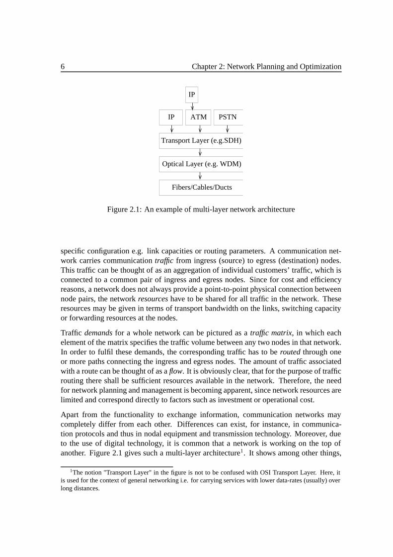
Figure 2.1: An example of multi-layer network architecture
specific configuration e.g. link capacities or routing parameters. A communication net-work carries communicationtraffic from ingress (source) to egress (destination) nodes.This traffic can be thought of as an aggregation of individual customers’ traffic, which isconnected to a common pair of ingress and egress nodes. Since for cost and efficiencyreasons, a network does not always provide a point-to-point physical connection betweennode pairs, the networkresourceshave to be shared for all traffic in the network. Theseresources may be given in terms of transport bandwidth on the links, switching capacityor forwarding resources at the nodes.
Traffic demandsfor a whole network can be pictured as atraffic matrix, in which eachelement of the matrix specifies the traffic volume between any two nodes in that network.In order to fulfil these demands, the corresponding traffic has to berouted through oneor more paths connecting the ingress and egress nodes. The amount of traffic associatedwith a route can be thought of as aflow. It is obviously clear, that for the purpose of trafficrouting there shall be sufficient resources available in the network. Therefore, the needfor network planning and management is becoming apparent, since network resources arelimited and correspond directly to factors such as investment or operational cost.
Apart from the functionality to exchange information, communication networks maycompletely differ from each other. Differences can exist, for instance, in communica-tion protocols and thus in nodal equipment and transmission technology. Moreover, dueto the use of digital technology, it is common that a network is working on the top ofanother. Figure 2.1 gives such a multi-layer architecture1. It shows among other things,
1The notion "Transport Layer" in the figure is not to be confused with OSI Transport Layer. Here, itis used for the context of general networking i.e. for carrying services with lower data-rates (usually) overlong distances.

2.2: Network Planning and Management 7
that IP networks can make use of either ATM (Asynchronous Transfer Mode) or directlySDH (Synchronous Digital Hierarchy) networks. SDH networks in turn can use WDM(Wavelength Division Multiplexing) networks to deliver services2. A similar layering ar-chitecture can also be deployed for the PSTN (Public Switched Telephone Network). Inregard to this multi-layer architecture, it is useful to distinguish two types of networks: (i)traffic networks, where demands are stochastic in nature (e.g. packet, voice or high speedon-demand circuit); they have also the switching/routing capability to handle short-livedrequests on-demand; and (ii)transport networks, which provide high-data rate servicesthat are required to be set up on a semi-permanent or permanent basis. Note that in such amulti-layer architecture, each layer has its own definition of traffic, link capacity and nodefunctionality [PM04]. This dissertation is dealing with planning and management issuesin IP networks, which can be categorized as traffic networks. For dimensioning problems,as those to be addressed in Chapter 5, we also need to consider the underlying transportnetwork, since transport granularities are different from one type of transport network toanother.
2.2 Network Planning and Management
Network Planning and Management (NPM) addresses all activities related to the networkdevelopment and evolution. There are basically three NPM activities, which correspondto different time-scales [PM04]3:
• long-term (months to years) activities to design or extend the network in order tomeet demands and requirements for a long period of time. These include for exam-ple: topology design, node and link dimensioning, capacity expansion, routing andresilience planning.
• medium-term (days to weeks) activities, which cover a list of actions to achieve theconvergence towards the established long-term plans. Routing control (offline) canalso be seen as a medium-term activity, at which routing is reconfigured to meetservice requirements or to obtain a better network usage.
• short-term (real-time to hours) activities, which incorporate real-time operationssuch as packet level operations (marking, scheduling, policing, buffer manage-ment), restoration or online routing control.
Figure 2.2 shows a generic interaction model for the NPM activities both for traffic andtransport networks. Long and medium-term NPM activities consider the current and fore-
2We refer to [Tan03] for a comprehensive overview of these different types of networks.3Different and coarser time granularities can also be used, in particular when planning focuses on trans-
port networks as in [Rob99] and [DDT+00].
8 Chapter 2: Network Planning and Optimization
and Resource Management
Long−Term Activities
Medium−Term Activities Short−Term Activities
Routing Update VariousControls
Topology
Forecast,
Capacity Change
Marketing Input(e.g. new Customers)
TrafficData
(Statistics)
TrafficData
(Statistics)
Network
e.g. Network Design
e.g. (Near)Real Time Traffice.g. Offline ResourceManagement
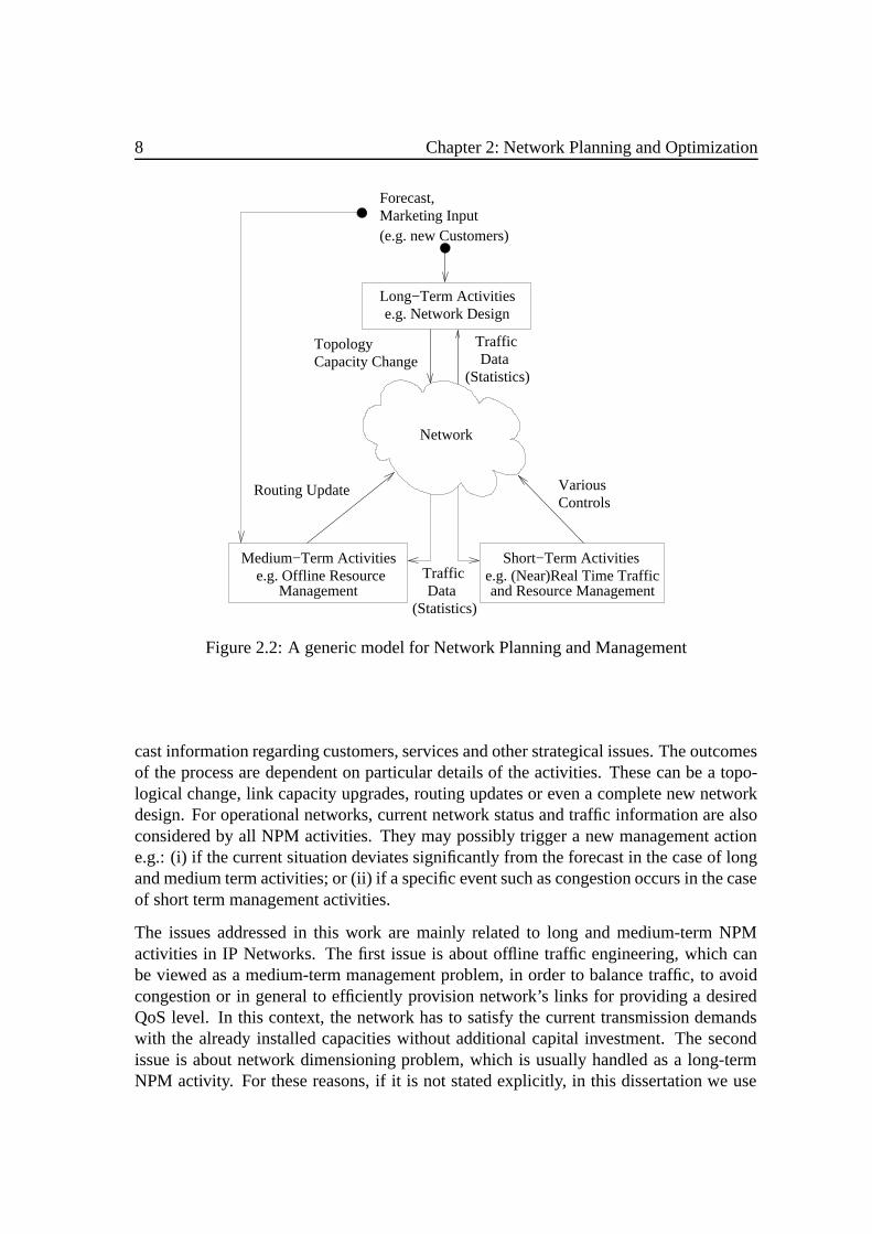
Figure 2.2: A generic model for Network Planning and Management
cast information regarding customers, services and other strategical issues. The outcomesof the process are dependent on particular details of the activities. These can be a topo-logical change, link capacity upgrades, routing updates or even a complete new networkdesign. For operational networks, current network status and traffic information are alsoconsidered by all NPM activities. They may possibly trigger a new management actione.g.: (i) if the current situation deviates significantly from the forecast in the case of longand medium term activities; or (ii) if a specific event such as congestion occurs in the caseof short term management activities.
The issues addressed in this work are mainly related to long and medium-term NPMactivities in IP Networks. The first issue is about offline traffic engineering, which canbe viewed as a medium-term management problem, in order to balance traffic, to avoidcongestion or in general to efficiently provision network’s links for providing a desiredQoS level. In this context, the network has to satisfy the current transmission demandswith the already installed capacities without additional capital investment. The secondissue is about network dimensioning problem, which is usually handled as a long-termNPM activity. For these reasons, if it is not stated explicitly, in this dissertation we use

2.3: Optimization Approaches 9
the term "planning and management" for the context of long and medium-term activities.
Each NPM activity is carried out in order to achieve certainobjectivesand fulfill somerequirements. Generally, these objectives and requirements can be in the form of eitherefficiency/performance measures or network’s cost. For long-term activities, the formeris usually taken as requirements and the latter as objectives. For medium-term activities,where no new capital investment is expected, the former is also used as objective. Inlarge network planning and design, networks have two types of cost: (i) CAPital EXpen-diture (CAPEX); and (ii) OPerational EXpenditure (OPEX). CAPEX refers to cost thatis primarily due to installation of capacity and equipment in the network while OPEXrefers to cost incurred due to operational needs of the network. Many design problemsare considered under either one or the other category. A network designer might devise aslick solution that can decrease CAPEX, but on the other hand, can increase OPEX dueto implementation complexity. In fact, there have been many cases where solutions thatsave CAPEX never made it to implementation in actual networks, simply because theyare too complicated to be deployed [PM04].
2.3 Optimization Approaches
In the area of Operations Research (OR), optimization is defined as a discipline whichis concerned with finding the maxima and minima of (objective) functions of many vari-ables, possibly subject to some constraints. The respresentation of an optimization prob-lem is often called asmathematical program. If the objective is a linear function, and theconstraints are linear equalities or inequalities, the corresponding mathematical programis called Linear Program (LP)4.
Most of planning and management problems in communication networks can be de-scribed bymulti-commodityflow models and mathematically formulated by linear ornon-linear systems. The term multi-commodity comes from the fact that there are multi-ple demands (or commodities) that need to be routed in the network simultaneously andthey compete for available resources (e.g. link capacities). Multi-commodity networkflow problems are frequentlypureLP problems as long as, roughly speaking, the objec-tive function is linear and bifurcated flows are allowed as independent decision variables.Such pure LP problems in most cases can be effectively solved to optimality using thewell knownsimplexalgorithm.
Unfortunately, many NPM problems are not pure LP problems, since (some) binary/ in-tegral variables are necessary to be included in the formulation due to technological orother restrictions. Solving such problems is far from trivial, and usually we can expect
4Sometimes we also use the acronym LP for Linear Programming.

10 Chapter 2: Network Planning and Optimization
with great likehood that the problems areNP-complete5 and intrinsically can not be solvedin an exact way in a reasonable time for large networks. In other words, in these cases,optimal solutions are frequently unreachable and one might use approximations to obtaingood, but not necessarily optimal, solutions. Such solution procedures are called heuris-tic methods or simplyheuristics. General heuristics that can be applied to many differentproblems are calledmeta-heuristics. They are basically high level concepts for exploringsolution spaces by using certain strategies, which are often non-deterministic (random-triggered). Furthermore, a heuristic that always takes the best immediate or local solutionwhile solving a problem is calledgreedyheuristic. Such a heuristic is usually problemspecific.
In this dissertation, heuristics are also used for cases where a problem can not be expressedas a linear program. This would generally mean that: (i) either such a problem is difficultto be expressed as a mathematical program; or (ii) the resulting formulation is non-linear.In the following subsections, we will discuss some of these approaches in more details.Special focus is put on those, which will be intensively used for solving the problemsconsidered in Chapters 4, 5 and 6.
2.3.1 Linear Programming
As stated earlier, a linear program is a mathematical model, in which the aim is to find aset of non-negative values for the unknowns or variables which maximize or minimize alinear equation or objective function, whilst satisfying a system of linear constraints. Alinear program in which some, but not all, of the variables are required to be integers, iscalled a Mixed Integer Linear Program (MILP). If it is required that all the variables areintegers, the corresponding linear program is called Integer Linear Program (ILP). Forminimizationproblems, a linear program6 can be expressed as follows:
minimize z =∑
j cjxj (2.1)
∑j aijxj ≤ bi, ∀i ∈ [1, m] (2.2)
xj ∈ R+, ∀j ∈ [1, n]
wherexj is thej-th decision variable,cj cost coefficient of variablej, aij coefficient forvariablej in constrainti, andbi right hand side of constrainti. An IP or a MIP can be
5In complexity theory, the NP-complete problems are the most difficult problems in the complexityclass NP (Non-deterministic Polynomial), in the sense that they are the ones most likely not to be in thecomplexity class P (Polynomial). A common and reasonably accurate assumption in complexity theory isthat "P" means "easy" and "not in P" means "hard". We refer to [Mar99], [PM04], [BG00] and [WIK05b]for formal definitions and further details of the complexity classes.
6Depending on the context, the notion "LP" is used both to point: (i) to the class oflinear program,which includes MILP and ILP; and also (ii) to thepure linear program i.e. without integrality constraints.
2.3: Optimization Approaches 11
obtained by constraining all or a certain set ofxj to be inZ+. Each set ofxj values forall values ofj that is compliant with the constraints, is called afeasiblesolution. Theoptimal solution is the feasible solution that minimizes the objective function.
Pure LP problems can be solved using the famoussimplexalgorithm. The set of all fea-sible solutions to a given LP problem is a convexpolytope7 formed by the intersection ofhyperplanes8, which are defined by the constraint equations. If a unique solution existsit is at a vertex of the polytope. To avoid labourous investigation of an excessive num-ber of vertices the simplex method provides a systematic computing scheme progressingfrom vertex to vertex in a direction of improving the objective function. Another popularsolving method for LP problems, known asInterior Point Method(IPM), was introducedsince the simplex method suffers from the exponential worst case behavior. However, formost practical applications, the simplex approach is proven to be very efficient.
Infeasible or Integer?
no
Bounding
Initialize;
Mark the node as inactive;
yes
Are there still active nodes?
Choose an active node;Mark the node as inactive;
END
Solve LP on these nodes;Branching(create 2 active nodes);
no
no
yes
yes
Solve LP relaxation of root node;
Infeasible or Integer?
Figure 2.3: The Branch and Bound algo-rithm
INFEA
z = −14(2 ; 2)INT
z = −13.5(1.5 ; 3)FRAC
x <= 31x >= 41
x <= 12 x >= 22
x <= 21x >= 31
x <= 22 x >= 32
A
B C
D E
F G
IH
z = −16.5(3.5 ; 1.5)FRAC
INFEAz = −16
FRAC(3 ; 1.75)
z = −13(3 ; 1)INT
z = −15.5
FRAC(2.5 ; 2)
(2 ; 2.25)FRAC
z = −15
Figure 2.4: An example of BB-tree
The standard algorithm for solving ILP and MILP problems is Branch and Bound (BB),which is basically a technique to speed upenumerationin a search tree. As indicated by
7A polytope can be thought of as the generalization to any dimension of polygon in two dimensions.8A hyperplane is an N-dimensional analogy of (two-dimensional) plane in (three-dimensional) space
and divides the N + 1 dimensional space into two half-spaces.
12 Chapter 2: Network Planning and Optimization
its name, two fundamental operations in BB are: (i) branching i.e. the process and thestrategy of creating two child subproblems from a parent problem; and (ii) bounding i.e.the process to get upper and lower bounds within a feasible subproblem. As an effectof branching, instead of solving the "difficult" parent problem, we try to solve a set of"easier" child subproblems. Futhermore, with the help of the established bounds, some ofthe child subproblems can be discarded. Lower bounds9 can be found e.g. byrelaxationtechniques. The LP relaxation of an ILP or a MILP is the linear program obtained by: (i)considering the same objective function; (ii) considering the same constraints; and (iii)relaxing the integrality property of the variables. The optimal value of the LP relaxationis the lower bound of the optimal value of the original ILP or MILP problem. Thus, if theoptimal solution of the LP relaxation is compliant with the integrality constraints , it isalso the optimal solution of the original ILP or MILP problem.
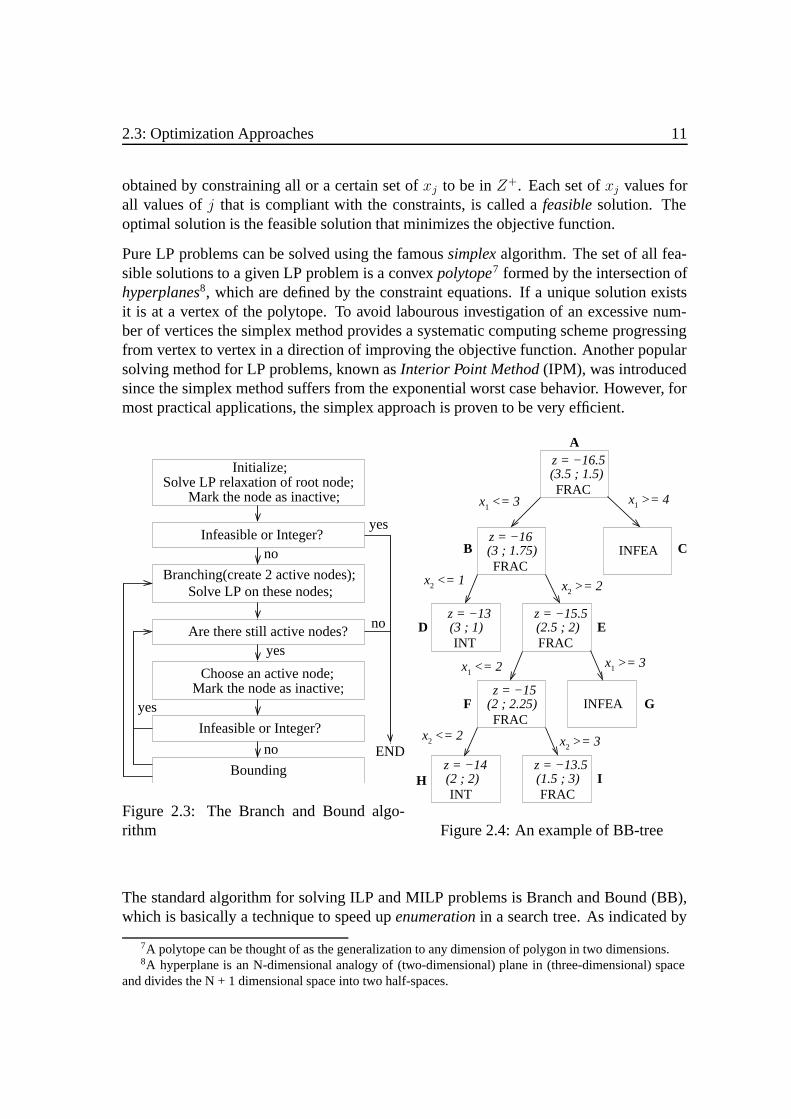
Figure 2.3 depicts the branch and bound algorithm. It will be explained by making use ofa BB-tree (as shown in Figure 2.4) for the following problem:
minimize z = −3x1 − 4x2
subject to 2x1 + 4x2 ≤ 13−2x1 + x2 ≤ 22x1 + 2x2 ≥ 16x1 − 4x2 ≤ 15xj ∈ Z+, ∀j ∈ 1, 2
At the beginning, the root node10 is defined and solved (e.g. by using the simplex al-gorithm). Since, as indicated by node A in Figure 2.4, the solution is fractional, i.e.(x1 = 3.5; x2 = 1.5), the algorithm will continue with branching. Suppose that we dobranching on variablex1 as shown in the figure, forming nodes B and C. Node C is in-feasible, while node B is fractional. Thus, node B is further processed. Since an integersolution is not yet found so far, the bounding procedure is not performed and the processis continued with branching. The results are nodes D and E. Now, node D is integer andused as temporary upper bound (best solution). Node E is fractional and processed bythe bounding procedure. In this case the lower bound at E(z = −15.5) is better thanthe current upper bound(z = −13). So it will again do branching, which yields nodes Fand G. Node G is infeasible and node F is fractional withz = −15 which is still betterthan the upper bound. Branching at F results in nodes H and I. Node H is integer, whichis better than the current upper bound. Thus it is adopted as the temporary upper boundvalue. Node I is fractional withz = −13.5 which is worse than the current upper boundwith z = −14. Hence, it will be discarded. Since there are no more active nodes, thealgorithm terminates and the temporary best solution is becoming the final solution of theproblem.
9As from now, if it is not explicitly stated, it is always assume that we considerminimizationproblems.10Note that anodein terminology of BB represents a subproblem, except the root node which represents
the original LP relaxation problem.
2.3: Optimization Approaches 13
Convex Hull
2
x1
LP Relaxation
x
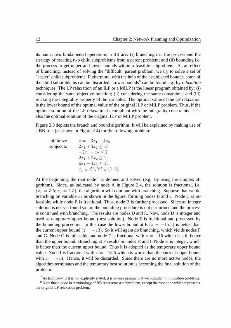
Figure 2.5: An illustration of feasible regions: LP relaxation vs. convex hull
Although the branch and bound approach can considerably reduce the number of sub-problems to be evaluated, the remaining number will often still be so large that it heavilyreduces the size of the problems that can be handled. The efficiency of BB depends onthe quality of the lower bounds obtained by solving node problems of the BB-tree. Ifthese bounds are close to the optimal integer solution then we can expect that the majorityof the nodes will never be visited as most of the BB-tree branches will not be entered.Therefore, it may happen that it is advantageous to spend more time in a node and try tofind a better lower bound than the one resulting from simple LP relaxation [PM04]. Thisis the basic idea behind an enhancement of BB technique calledBranch and Cut(BC).
The basic way to achieve better lower bounds is to constructvalid inequalitiesin theBB-tree nodes. Such inequalities are generated and inserted to problems, on top of thestandard constraints. The idea is to exploit the integrality of variables in order to produceinequalities that are valid for all integral solutions and at the same time remove partsof the polytope which contains non-integral optimal solutions. It is also desirable thatsuch inequalities define the faces (facets)11 of theconvex hull12 of the solution set for theoriginal problem. For clarity, Figure 2.5 shows the depiction of the feasible regions of anLP relaxation and of a convex hull of the non-relaxed problem. If we can find a set ofvalid inequalities defining the convex hull of a problem, the corresponding problem canbe solvedeasilysince the solution of an LP for the transformed problem will always be afeasible solution of the original MILP/ILP problem.
For solving the problems addressed in this dissertation, insofar LP, MILP or ILP are con-cerned, a commercial solver tool called CPLEX [CPL01] is used. For MILP and ILP
11A facet is a part of a hyperplane, forming a boundary for a polytope.12A convex hull is the smallest polytope containing all feasible solutions of the non-relaxed version of a
problem.

14 Chapter 2: Network Planning and Optimization
problems, it exploits a (type of) branch and cut algorithm. Since it is a general solver, thecuts(i.e. valid inequalities) added to the model are also very general (we refer to [CPL01]for the details) i.e. CPLEX does not exploit specific structures of the considered problem.There are currently many publications addressing the issue of performing specific cuts forspecific problems. However, such an approach is beyond the scope of this dissertation.
2.3.2 Greedy Heuristics
Greedy Algorithm for Routing Problemfor all demandsd ∈ D do
determine all possible routesRd;for all possible router ∈ Rd do
calculate incremental cost for assignmentd to r;end forselect router with the lowest cost;establish demandd on the chosen router;
end for
Figure 2.6: A greedy algorithm for routing problem
Greedy heuristics are simple and straightforward. They are called "greedy", in the sensethat in each algorithm step they take decisions on the basis of information at hand withoutregard for future consequences. In other words, in each phase the algorithms decide fora local optimumin the hope that at the end they reach anear if not a global optimalso-lution. The main benefit of such algorithms is, that they can construct a feasible solutionvery fast. Figure 2.6 gives an example of a greedy algorithm for solving network’s routingproblem, in order to minimize a certain cost parameter. It basically tries for each elemen-tary demandd to assign a router, which is optimal at the time the allocation is done (i.e.locally optimal). Surely, with this allocation strategy, an end result is very much depen-dent on thesequence, in which the demand poolD is processed. And by using such amechanism (as a part) in our optimization procedure, we essentially transform our prob-lems tosequential ordering problems(SOPs). The effectiveness of such an approach hasbeen previously investigated for example in [Bec01].
2.3.3 Plain Local Search
Local search is a meta-heuristic search algorithm, which is based on the concept ofneigh-borhood. A neighborhood of a solution vectorx is a set of solutions that are in somesense close tox, for example because they can be easily computed fromx or because they
2.3: Optimization Approaches 15
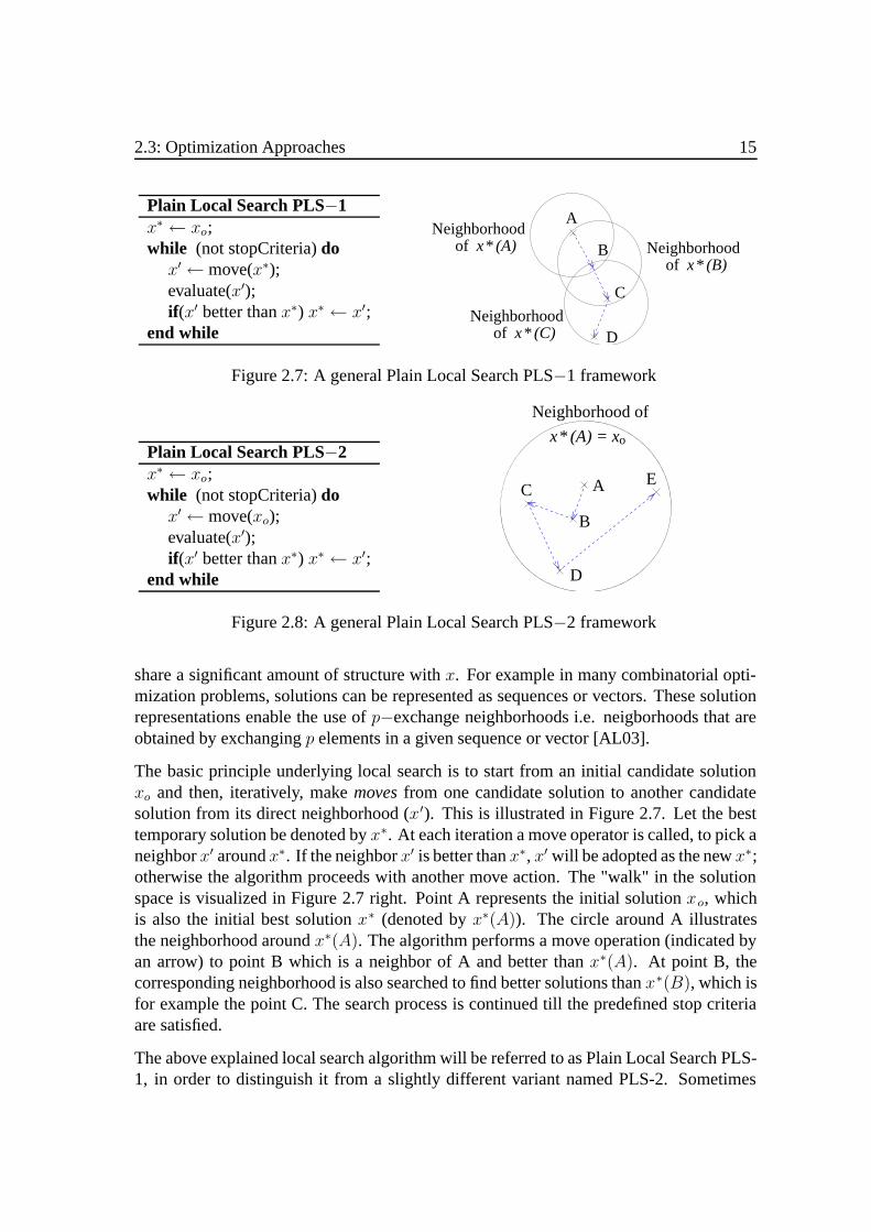
Plain Local Search PLS−1x∗ ← xo;while (not stopCriteria)dox′ ←move(x∗);evaluate(x′);if (x′ better thanx∗) x∗ ← x′;
end while
C
*
D
x (A)
x (C)*
x (B)*B Neighborhood
Neighborhood
Neighborhoodof
of
of
A
Figure 2.7: A general Plain Local Search PLS−1 framework
Plain Local Search PLS−2x∗ ← xo;while (not stopCriteria)dox′ ←move(xo);evaluate(x′);if (x′ better thanx∗) x∗ ← x′;
end while
Neighborhood of
*x (A) = xo
B
C
D
EA
Figure 2.8: A general Plain Local Search PLS−2 framework
share a significant amount of structure withx. For example in many combinatorial opti-mization problems, solutions can be represented as sequences or vectors. These solutionrepresentations enable the use ofp−exchange neighborhoods i.e. neigborhoods that areobtained by exchangingp elements in a given sequence or vector [AL03].
The basic principle underlying local search is to start from an initial candidate solutionxo and then, iteratively, makemovesfrom one candidate solution to another candidatesolution from its direct neighborhood (x′). This is illustrated in Figure 2.7. Let the besttemporary solution be denoted byx∗. At each iteration a move operator is called, to pick aneighborx′ aroundx∗. If the neighborx′ is better thanx∗, x′ will be adopted as the newx∗;otherwise the algorithm proceeds with another move action. The "walk" in the solutionspace is visualized in Figure 2.7 right. Point A represents the initial solutionxo, whichis also the initial best solutionx∗ (denoted byx∗(A)). The circle around A illustratesthe neighborhood aroundx∗(A). The algorithm performs a move operation (indicated byan arrow) to point B which is a neighbor of A and better thanx∗(A). At point B, thecorresponding neighborhood is also searched to find better solutions thanx∗(B), which isfor example the point C. The search process is continued till the predefined stop criteriaare satisfied.
The above explained local search algorithm will be referred to as Plain Local Search PLS-1, in order to distinguish it from a slightly different variant named PLS-2. Sometimes
16 Chapter 2: Network Planning and Optimization
1st Neighborhood
3rd Neighborhood
*x (A) = xo
2nd Neighborhood
B
C A E
D
F
of
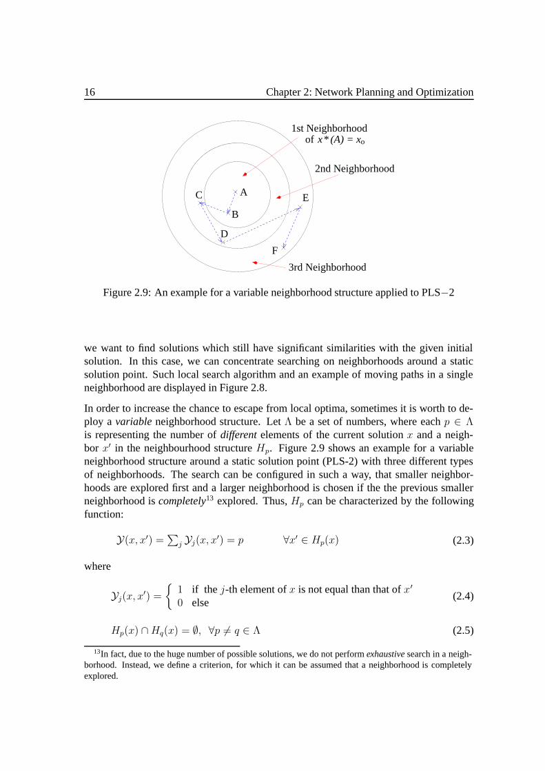
Figure 2.9: An example for a variable neighborhood structure applied to PLS−2
we want to find solutions which still have significant similarities with the given initialsolution. In this case, we can concentrate searching on neighborhoods around a staticsolution point. Such local search algorithm and an example of moving paths in a singleneighborhood are displayed in Figure 2.8.
In order to increase the chance to escape from local optima, sometimes it is worth to de-ploy a variable neighborhood structure. LetΛ be a set of numbers, where eachp ∈ Λis representing the number ofdifferentelements of the current solutionx and a neigh-bor x′ in the neighbourhood structureHp. Figure 2.9 shows an example for a variableneighborhood structure around a static solution point (PLS-2) with three different typesof neighborhoods. The search can be configured in such a way, that smaller neighbor-hoods are explored first and a larger neighborhood is chosen if the the previous smallerneighborhood iscompletely13 explored. Thus,Hp can be characterized by the followingfunction:
Y(x, x′) =∑
j Yj(x, x′) = p ∀x′ ∈ Hp(x) (2.3)
where
Yj(x, x′) =
1 if the j-th element ofx is not equal than that ofx′
0 else(2.4)
Hp(x) ∩Hq(x) = ∅, ∀p = q ∈ Λ (2.5)
13In fact, due to the huge number of possible solutions, we do not performexhaustivesearch in a neigh-borhood. Instead, we define a criterion, for which it can be assumed that a neighborhood is completelyexplored.
2.3: Optimization Approaches 17
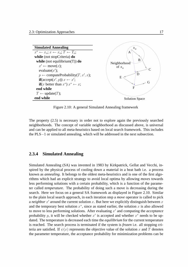
Simulated Annealingx∗ ← xo; x← xo; T ← To;while (not stopCriteria)dowhile (not equilibrium(T))dox′ ←move(x);evaluate(x′);p← computeProbability(T, x′, x);if (accept(x′, p)) x← x′;if (x better thanx∗) x∗ ← x;
end whileT ← update(T );
end while
F
Neighborhood
A
of
xo
xo
Solution Space
B
CD
E
G
Figure 2.10: A general Simulated Annealing framework
The property (2.5) is necessary in order not to explore again the previously searchedneighborhoods. The concept of variable neighborhood as discussed above, is universaland can be applied to all meta-heuristics based on local search framework. This includesthe PLS−1 or simulated annealing, which will be addressed in the next subsection.
2.3.4 Simulated Annealing
Simulated Annealing (SA) was invented in 1983 by Kirkpatrick, Gellat and Vecchi, in-spired by the physical process of cooling down a material in a heat bath i.e. a processknown asannealing. It belongs to the oldest meta-heuristics and is one of the first algo-rithms which had an explicit strategy to avoid local optima by allowingmovestowardsless performing solutions with a certain probability, which is a function of the parame-ter calledtemperature. The probability of doing such a move is decreasing during thesearch. Here we focus on a general SA framework as displayed in Figure 2.10. Similarto the plain local search approach, in each iteration step amoveoperator is called to pickaneighborx′ around the current solutionx. But here we explicitly distinguish betweenxand the temporary best solutionx∗, since as stated earlier, the solutionx is also allowedto move to less performing solutions. After evaluatingx′ and computing theacceptanceprobabilityp, it will be checked whetherx′ is accepted and whetherx∗ needs to be up-dated. The temperature is decreased each time theequilibriumfor the current temperatureis reached. The search process is terminated if the system isfrozeni.e. all stopping cri-teria are satisfied. Ifψ(x) represents the objective value of the solutionx andT denotesthe parameter temperature, the acceptance probability for minimization problems can be

18 Chapter 2: Network Planning and Optimization
expressed as follows:
p =
1 if ψ(x′) < ψ(x)
exp(−ψ(x′)−ψ(x)T
) if ψ(x′) ≥ ψ(x)(2.6)
It simply says that: (i) if the neigborx′ is better than the current solutionx (i.e. ψ(x′) <ψ(x)), thenx will be updated byx′; (ii) if the neighbor is worse than the current solution,x′ can still be accepted asx with the probabilityp; and (iii) the lower the temperature(i.e. the longer the algorithm’s running time) and the worse the quality of the neighbor,the lower the value ofp. An abstract visualization for themovingpath in the solutionspace for simulated annealing is depicted in Figure 2.10 right. Two paths are available inthe figure, indicating the moving path for the temporary current solutionx (i.e. the pathA-B-C-D-E-F-G) and that for the temporary best solutionx∗ (i.e. the path A-D-F). Ascan be seen in the Figure, during the search,x can leave the best temporary solutionx∗
and not find it again.
Temperature
The starting temperatureT shall enable that in the beginning nearly all perturbations areaccepted. In practice,T can be chosen as the objective value of the initial solution i.e.:
To = ψ(xo) (2.7)
A cooling schedule(updating rule) for the temperature could be in the form of:
Tk+1 = γ · Tk (2.8)
whereTk is the current temperature,Tk+1 is the temperature of the next iteration andγ is a decreasing factor less than 1. At the end,T should be so small that only a verysmall number of perturbations is accepted i.e. almost only improving solutions should beaccepted.
Equilibrium and Frozen State
Equilibrium and frozen state can be defined according to some parameters. The easiestway is by using a simple and general criterion such as a predefinednumber of iterations.Note that the equilibrium state is measured only for a constant temperature value, whilethe frozen state for the whole process. Several other parameters can also be used incombination with a maximum number of iterations e.g.: (i) ifψ(x∗) is not improved atleastε% afterK1 iterations; or (ii) if the number ofacceptedmoves is less thanε% ofthe lastK2 iterations (recall that a move will be accepted on a random basis dependingon the probability valuep). Furthermore, for the frozen state we could also look at thetemperature value e.g. when the temperature gets below a predefined constantTmin thesystem is assumed to be frozen.

2.3: Optimization Approaches 19
2.3.5 Genetic Algorithms
no
Regeneration
CrossoverMutation
Parents Selection
Initialize Population
Stop Criteria fulfilled ?
ENDyes
Survivors Selection
Figure 2.11: A general Genetic Algo-rithm framework
(best 50 chromosomes)
50 Chromosomes
Population
Population
Selection(remove 10%)
45 Chromosomes
Selection (parents)
10 Chromosomes
Offsprings10 Chromosomes
SelectionPopulation55 Chromosomes
CrossoverMutation
Figure 2.12: An example of population dy-namics
Genetic Algorithms (GAs) were introduced by Holland in 1975, inspired by nature’s capa-bility to evolve individuals influenced by adaptation to the environment. In the optimiza-tion context, genetic algorithms use the concepts from population genetics and evolutiontheory in order to optimize thefitnessof a populationof individuals throughrecombi-nation (crossover) andmutationof their genes. Figure 2.11 shows a block diagram of acommon GA implementation. At first, a solution in the problem domain has to be ap-propriatelyencodedand transformed to achromosome14 in GA domain. The encodingmechanism is usually problem specific i.e. it depends much on the problem under con-sideration. At the beginning of the algorithm, the population has to be initialized i.e.some individuals or chromosomes have to be generated randomly or according to a cer-tain rule. After this, the evolution phase is taking place. The evolution consists of somemechanisms to performselectionand to form new individuals using genetic operatorscalledcrossoverandmutation. Generally, crossover is intended to exploit the structurepresent in the available (good performing) individuals, while mutation is used to increasethe capability to explore the solution space without getting stuck in local optima. Bothof these genetic operators aim at producing some (hopefully) better individuals for thenext iteration. The least successful individuals (according to their fitness parameter) fromthe previous iteration willnaturallybe removed and then be substituted by the new ones.Applying the described processes in many iterations we continously improve the averagequality of the solutions until the predefined stopping criteria are met. As in PLS and SA
14Throughout this dissertation we use the terms "chromosome" and "individual" interchangeably.

20 Chapter 2: Network Planning and Optimization
frameworks, the stopping criteria can be derived from the standard parameters: the maxi-mum number of iterations, the improvement status ofψ(x∗) or their combination. In whatfollows, some general implementation issues will be discussed.
Population Dynamics
There are no standardized rules to decide how many chromosomes should be in the pop-ulation, since the size of the population is not directly correlated with the quality of thesolutions. Figure 2.12 shows an example of population dynamics in a genetic algorithm.The size of the population is hold constantly at 50 individuals. Some of them, in thiscase 10 individuals, are selected as parents of the new individuals. Survivors of currentgeneration are then selected by removing several individuals. After that, the populationfor the next generation is constructed by applying once again the selection mechanism,holding the population size the same as the previous generation.
Selection
Selection is done based on fitness. There are basically two selection mechanisms: (i)parents selection to get some parent individuals for a new generation; and (ii) survivorsselection, which is intended to keep best individuals within the population and remove acertain number of the least performing individuals in the current generation. For parentsselection we should find a strategy that: (i) ideally gives better individuals a better chanceof being parents than less good individuals; and (ii) also gives less good individuals atleast some chance of being parents, as they may provide some useful genetic material.This task can be fulfilled by a so-calledrank selection: individuals in the population areranked and each of them receives a probability value (to be selected) from this ranking.The probability value is measured relative to the probability value of the last (i.e. worst)individual; this means the last but one will have twice that probability etc. Of course thesevalues have to be normalized such that the sum of these probability values must equalone. Afterwards, the probability values are mapped on the corresponding non overlappingintervals in the range[0, 1] and a randomly chosen number in this interval is used to selectan individual. For survivors selection, we can simply sort the individuals according totheir fitness from best to worst and then remove some of the least performing individuals.
Forming New Individuals
New individuals are generated by two standard GA operators: crossover and mutation.Crossover produces new individuals thatinherit genes from their parents. On the otherhand, mutation enables offsprings to have different genes as those from their parents.

2.3: Optimization Approaches 21
SA / GA PLS
1
10
0
Figure 2.13: A hybridization scheme between SA/GA and PLS
Since both crossover and mutation are dependent on how a chromosome is encoded, de-tails of such mechanisms are also problem specific and can not be discussed until theproblem and the corresponding encoding mechanism are defined.
2.3.6 Hybridization
Each optimization approach mentioned above has its own advantages. Therefore, it issometimes worth to make a hybridization of two or more approaches, combining theiradvantages together. In this subsection, two types of hybridization will be introduced.Firstly, we combine PLS together with SA or GA. PLS is very simple and usually hasa good convergence behavior i.e. for relatively short execution time it can find goodsolutions. Unfortunately, it can also get stuck in local optima, simply because it hasno explicit mechanism to avoid such a situation. On the other hand, SA or GA basedapproaches are theoretically able to explore a larger solution space and thus to avoid localoptima. But they have a relatively slower convergence behavior. The basic idea behindthe hybridization is illustrated in Figure 2.13. It shows the execution process of PLS orSA/GA as a function of a boolean variableσPLS, which indicates whether a condition forperforming PLS is satisfied (σPLS = 1) or not (σPLS = 0).
In the case of SA-PLS approach, this hybridization can easily be performed in anormalSA approach, by modifying the acceptance probability as follows:
p =
1 if ψ(x′) < ψ(x)
exp(−ψ(x′)−ψ(x)T
) if ψ(x′) ≥ ψ(x)andσPLS = 00 otherwise
(2.9)
This means ifσPLS = 1, the probabilityp will have the value of 1 if the neighborx′ isbetter thanx, and the value of 0 ifx′ is worse thanx. This is the behavior of PLS. ForσPLS = 0 equation (2.9) is equivalent to (2.6). Note that for a quite low temperaturevalue, which is roughly equivalent with a long execution time, a normal SA behavesapproximately like PLS. Thus, this modification mainly effects the SA characteristics athigh temperature values.

22 Chapter 2: Network Planning and Optimization
(best 50 Chr.)
Population
45 ChromosomesPopulation
Search result
55 or 56 Chromosomes
(1 or 0 Chr.)
PLSCrossoverMutation
1 Chromosome
Selection (parents)10 Chr.
Selection
Population50 Chromosomes
(remove 10%)
10 Chr.Offsprings
Selection
Figure 2.14: Population dynamics in a hybrid GA-PLS scheme
For the case of GA-PLS approach, it is a bit more complicated, mainly because geneticalgorithm is a population based (multi-agent) approach, while PLS is asingle-agentap-proach. One possibility is to construct a quasi parallel PLS process at a certain GA evo-lution cycle (iteration), where the variableσPLS has the value of 1. This possibility isdisplayed as a part of population dynamics in Figure 2.14 (cf. Figure 2.12). Here, anindividual is selected from a number of best individuals in the population and used asinput for the PLS process. If PLS is able to find a better solution (than the original inputindividual), it will be sent to the population as a new individual.
Note that for such hybrid approaches, the PLS function is active ifσPLS = 1. In bothSA-PLS and GA-PLS approaches, this activation can base on the simple criteria such as:(i) if a certain number of iteration is reached; or (ii) if the best temporary solutionx∗ isjust improved. Furthermore, in simulated annealing it is also possible to activate PLS, ifthe neighborhood aroundx∗ is not yetcompletelyexplored.
Due to the huge number of possible solutions, performance of stochastic search ap-proaches is sometimes still far from expectation e.g. in terms of convergence or solu-tion quality. But often, the existence of simpleproblem-specificheuristics can improveperformance a lot. In this regard, a hybridization between such a simple heuristic anda stochastic search algorithm is of particular importance. Figure 2.15a gives a generaldiagram of a hybrid algorithm, which makes use of simple improving heuristics. Searchalgorithms meant in the diagram are stochastic search algorithms e.g. PLS, SA, GA, SA-

2.3: Optimization Approaches 23
Algorithm
Solution e.g. in terms of aSequence of Demands
(b)
Improving
Improved Solution
Solution
(a)
SearchAlgorithm
Simple
Heuristic
GreedyHeuristic
Search
Objective Value
Figure 2.15: Hybridization of general search algorithms with simple heuristics
PLS, GA-PLS or others. A simple improving heuristic takes a solution from the searchalgorithm and tries to improve that solution (stochastically or deterministically). Thus, inlocal search terminology for instance, it can be adopted as a new type of (in addition toa standardrandom) move operator. In Figure 2.15b another hybrid algorithm is depicted.Here, a greedy heuristic is used in order tointerpret andassessa solution produced bythe stochastic search algorithm. In the case of network routing problems, an examplewould be that the search algorithm optimizes the sequence in which the greedy heuristicprocesses the demands. Thus, the applicability of this kind of hybridization is stronglyrelated to how a solution is represented inside the stochastic search algorithm and howthe information contained in a solution can be used by the greedy heuristic to constructanactualsolution. Such a hybridization, as reported in [Bec01] has several benefits: (i)a greedy heuristic is typically simple and can always produce feasible solutions; (ii) thesolution space to be explored is usually (much) smaller compared to the original solutionspace, where the stochastic search algorithm is performed without greedy heuristics; thismight increase the performance of the search algorithm. The latter is a also direct impactof the problem transformation, as implicitly stated by using greedy heuristics. For ex-ample, consider a network’s routing problem with10 node-pairs, each has10 candidatepaths. The solution space contains1010 possible solutions. If we now use the greedyheuristic as discussed in Subsection 2.3.2 and encode a solution as a specific sequence ofdemands, in which they are processed by the greedy heuristic then the current solutionspace now contains10! possible solutions. Unfortunately, this mechanism sometimes willintroduce problems. As the search process is reduced to a certain area of the (original) so-lution space, several good or optimal solutions might be excluded. However, as has beenshown in [Bec01], due to the largeness of the solution space in most planning problemsin communication networks, such a problem happens rarely.

24 Chapter 2: Network Planning and Optimization

Chapter 3
Overview of IP Routing
The Internet is a large network that connected about 160 million hosts (in June 2002)1,which are organized in about 13,000 distinct domains2, called Autonomous Systems(ASes) [QPS+03]. With the decommissioning of the NSFNet3 Internet backbone net-work in 1995, the Internet now functions with no single central network at all and en-tirely consists of the various commercial Internet Service Providers (ISPs), private net-works and Research and Education Networks (RENs), as connected at their peering points[WIK05a]. Global connectivity is provided by so-called Tier-1 ISPs; these represent thehighest hierarchy level of the network and exchange traffic to each other on a revenue-neutral basis (i.e. a Tier-1 ISP does not pay for transit on other Tier-1 ISP networks).
An AS has its ownroutersand routing policies, and connects (peers) to other ASes toexchange traffic with remote hosts. A peering link could connect to a public InternetExchange Point (IXP), or directly to a private peer or transit/upstream provider. Insidean AS, the network can be viewed as a directed graph, where nodes and arcs representrouters and IP links, respectively. A typical ISP network architecture is depicted in Figure3.1. Since an ISP usually offers services at several places, geographically the networkconsists of several Point-of-Presences (PoPs) where a set of routers is maintained. Froma simplified perspective, a network consists of a combination of Core Routers (CRs) con-nected to other PoPs, Border Routers (BRs) connected to other ASes, Hosting Routers(HRs) connected to media servers, and Access Routers (ARs) connected directly to cus-tomers [XTF+02]. In an operational network, this split in functionality simplifies therequirements for each router. For example: (i) an AR should provide high port density toconnect to a large number of customers with various access speeds and technologies; (ii) aCR should provide high packet forwarding performance; etc. Furthermore, isolating peer
1In January 2005 it increased to more than 310 million hosts [ISC05].2A domain corresponds roughly to one company or one Internet Service Provider.3NSFNet stands for National Science Foundation Network, which was the scientific research and edu-
cation network in the USA.
25

26 Chapter 3: Overview of IP Routing
Access Links
CR: Core RouterHR: Hosting RouterBR: Border RouterAR: Access Router
HR
HR
CR
CRAR
AR
CR
CR
HR
BR CR
CR
AR
CR
CRBRPoP
Peering Links
PoP: Point of Presence
Figure 3.1: A typical ISP architecture
traffic to a small set of BRs simplifies the management of inter-domain routing policies[FGL+00].
Currently, Internet routing is handled by two distinct protocols: Exterior Gateway Pro-tocol (EGP) and Interior Gateway Protocol (IGP). On one hand, EGP is used for routingbetween ASes, distributing reachability information and selecting the best route to eachdestination that is compatible with the routing policies of the transit domains withoutknowing their topology. The Border Gateway Protocol (BGP) is the current de factostandard inter-domain routing protocol. On the other hand, IGP handles routing inside asingle domain, determines the best route to reach each internal subnetwork or host, basedon some metrics (e.g. delay, bandwidth). The most commonly used IGPs todays are OpenShortest Path First (OSPF) and Intermediate System to Intermediate System (IS-IS).
To increase routing flexibility and provide QoS in IP networks, several new enhancementshave recently been proposed. There are two technologies which are of paramount impor-tant and likely to be a common standard for IP networks in providing better services inthe near future. These are Multi-Protocol Label Switching (MPLS) and DifferentitatedServices (DiffServ). MPLS provides a basic means to efficiently steer IP traffic, whileDiffServ gives the possibility to differentiate treatments for IP packets with respect totheir class of service. Both will be addressed later on in this chapter.
In this dissertation we only focus on intra-domain routing, including MPLS. Surely,
3.1: Classical IP Networks 27
MPLS can also be applied for inter-domain routing, but the use of such a mechanismis still problematic. This is because each ISP is administratively independent, and inter-domain coordination is in practice very difficult to realize.
The rest of this chapter is organized as follows. Section 3.1 describes routing inclassicalIP networks. Here, the term "classic" is used to refer to IP networks that route traffic usingan IGP. In Section 3.2 MPLS is briefly reviewed. Finally, Section 3.3 reveals the DiffServarchitecture and the corresponding impacts on routing in the network.
3.1 Classical IP Networks
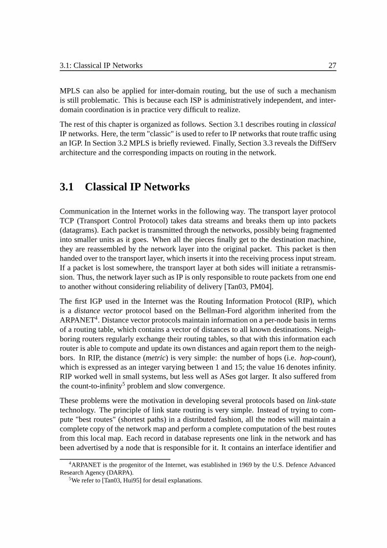
Communication in the Internet works in the following way. The transport layer protocolTCP (Transport Control Protocol) takes data streams and breaks them up into packets(datagrams). Each packet is transmitted through the networks, possibly being fragmentedinto smaller units as it goes. When all the pieces finally get to the destination machine,they are reassembled by the network layer into the original packet. This packet is thenhanded over to the transport layer, which inserts it into the receiving process input stream.If a packet is lost somewhere, the transport layer at both sides will initiate a retransmis-sion. Thus, the network layer such as IP is only responsible to route packets from one endto another without considering reliability of delivery [Tan03, PM04].
The first IGP used in the Internet was the Routing Information Protocol (RIP), whichis a distance vectorprotocol based on the Bellman-Ford algorithm inherited from theARPANET4. Distance vector protocols maintain information on a per-node basis in termsof a routing table, which contains a vector of distances to all known destinations. Neigh-boring routers regularly exchange their routing tables, so that with this information eachrouter is able to compute and update its own distances and again report them to the neigh-bors. In RIP, the distance (metric) is very simple: the number of hops (i.e.hop-count),which is expressed as an integer varying between 1 and 15; the value 16 denotes infinity.RIP worked well in small systems, but less well as ASes got larger. It also suffered fromthe count-to-infinity5 problem and slow convergence.
These problems were the motivation in developing several protocols based onlink-statetechnology. The principle of link state routing is very simple. Instead of trying to com-pute "best routes" (shortest paths) in a distributed fashion, all the nodes will maintain acomplete copy of the network map and perform a complete computation of the best routesfrom this local map. Each record in database represents one link in the network and hasbeen advertised by a node that is responsible for it. It contains an interface identifier and
4ARPANET is the progenitor of the Internet, was established in 1969 by the U.S. Defence AdvancedResearch Agency (DARPA).
5We refer to [Tan03, Hui95] for detail explanations.

28 Chapter 3: Overview of IP Routing
information describing the state of the link: the destination and the distance (also calledaslink cost, metricor weight). With this information, by using Dijkstra’s algorithm, eachnode can easily compute the shortest path from itself to all other nodes. As all nodes havethe same database, the routes are coherent and loops cannot occur [Hui95].
Today, the main IGP protocols are OSPF and IS-IS, which belong to link-state protocols.IS-IS is actually very similar to OSPF, but it has been specified by the International Or-ganization for Standardization (ISO). Compared to RIP, OSPF is in general much morecomplex. OSPF supports a variety of distance metrics e.g. physical distance, delay orcost. However, for path computation only one metric is used at a time. It also allowshierarchical routing and is more stable (faster convergence). Therefore, it is used in largernetworks such as enterprise and ISP internal networks. For the rest of this dissertation,we always use the term "IGP" mainly to refer to "OSPF". Otherwise it will be statedexplicitly. In the following paragraphs, we will review the routing mechanism facilitatedby IGP to provide a basis for our traffic engineering approach, which will be addressed innext chapter. Our interest is mainly on data-plane operations6.
An IP datagram consists of a header and a data part. The header has a 20-byte fixed partand a variable length optional part. The header consists of several pre-defined fields. Inthe context of routing, only thedestination addressfield is of prominent interest, sincepackets are routed based on their destinations. An extended feature to support routingbased on class of service as specified in theType of Service(ToS) field is in practicerarely used. It does not play any substantial role until the introduction of MPLS andDiffServ (see Section 3.3).
The main advantage of shortest path routing is that it can be implemented in a distributedway, in a form known as (connectionless) hop-by-hop destination based routing. Figure3.2 gives an example of such a routing mechanism. Assume that we have a six-routernetwork which is configured as displayed in Figure 3.2a. Router 1 connects to network A,whilst router 5 and router 6 to network B and network C, respectively. Each router main-tains the complete network map and computes shortest paths to all destinations, whichin turn are used for constructing a routing table consisting of next hop and interface7
information. Figures 3.2b and 3.2c show an example of the shortest path tree and thecorresponding routing table seen from router 1. If a packet arrives at a certain router, itwill look at the destination address and forward the packet to the correct outgoing inter-face as specified by its routing table. This illustrates in Figure 3.2d. Two packets withdestinations B4 (representing host number 4 inside network B) and C1 (representing hostnumber 1 inside network C) arrive at router 1, will be forwarded to router 3. Since router 3also has a routing table derived from the same network map, it knows that the packet with
6Routing has two types of operations: data-plane and control-plane operations. The data-plane opera-tions are those that are performed on every packet whereas the control-plane sets up information to facilitatedata-plane operations (e.g. routing table).
7A link may consist of several interfaces.

3.1: Classical IP Networks 29
Destination Next Hop Interface
B4
C1
B4
C1
B4
C1
6
5
3
C
2 A
1 2
43
5 6
1
1 2
4
5 6
network A
network B network C
5
53
2
1 2
2
A
B
C
direct
3
3
1−A
1−3
1−3
3
(a) (b)
(c)
(d)
4
B
C1
C1B4
Figure 3.2: Hop-by-hop destination-based IP routing
destination network B must be forwarded to router 5 and that with destination network Cto router 4. This process continues till those packets reach their destination hosts.
In OSPF networks, it is possible, to some extent, to do load balancing. Using the so-calledEqual-Cost Multi-Path (ECMP) rule, if there are multiple shortest paths to a particulardestination, the corresponding traffic is equally split over the outgoing links belongingto these shortest paths. In practice, the split may not exactly follow ECMP; that is, thesplit decision is not done on a packet-by-packet basis in a round robin manner amongthe multiple outgoing links that coincide with the (multiple) shortest paths [PM04]. Thisis because such a mechanism may introduce packet disordering problems, which can inmany cases lead to performance degradation that is not easy to overcome. Therefore thefollowing load balancing schemes are generally recommended:
• destination based load balancing i.e. in the case of multiple shortest paths, traffic
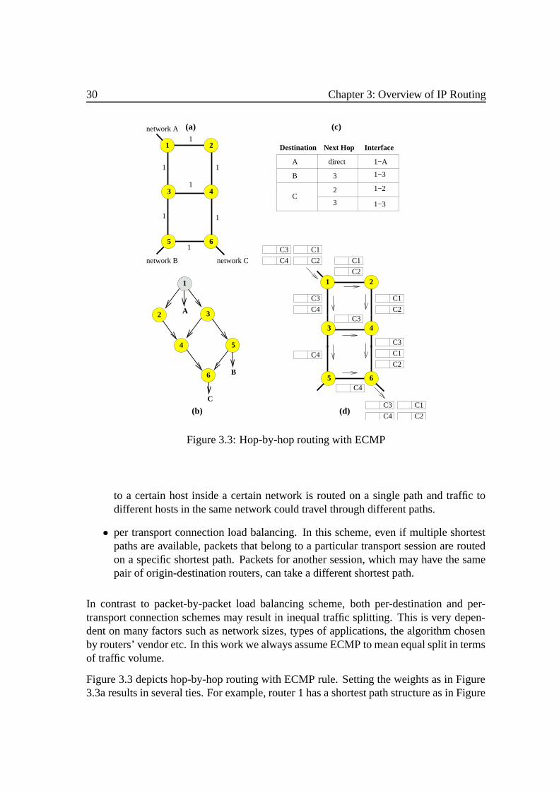
30 Chapter 3: Overview of IP Routing
Destination Next Hop Interface
C2
C3
C4 C2
C1
C3
C4
C4
C3
C3
C4
C1
C2
C1
C2
C1
C2
6
1 2
43
5 6
network A
network B network C
1
11
1
1 1
1
(a)
6
3
(d)
A direct 1−A
3 1−3
2 1−2
B 3 1−3
C
(c)
(b)
1
2 3
4 5
A
C
B
1 2
4
5
C3
C4
C1
Figure 3.3: Hop-by-hop routing with ECMP
to a certain host inside a certain network is routed on a single path and traffic todifferent hosts in the same network could travel through different paths.
• per transport connection load balancing. In this scheme, even if multiple shortestpaths are available, packets that belong to a particular transport session are routedon a specific shortest path. Packets for another session, which may have the samepair of origin-destination routers, can take a different shortest path.
In contrast to packet-by-packet load balancing scheme, both per-destination and per-transport connection schemes may result in inequal traffic splitting. This is very depen-dent on many factors such as network sizes, types of applications, the algorithm chosenby routers’ vendor etc. In this work we always assume ECMP to mean equal split in termsof traffic volume.
Figure 3.3 depicts hop-by-hop routing with ECMP rule. Setting the weights as in Figure3.3a results in several ties. For example, router 1 has a shortest path structure as in Figure
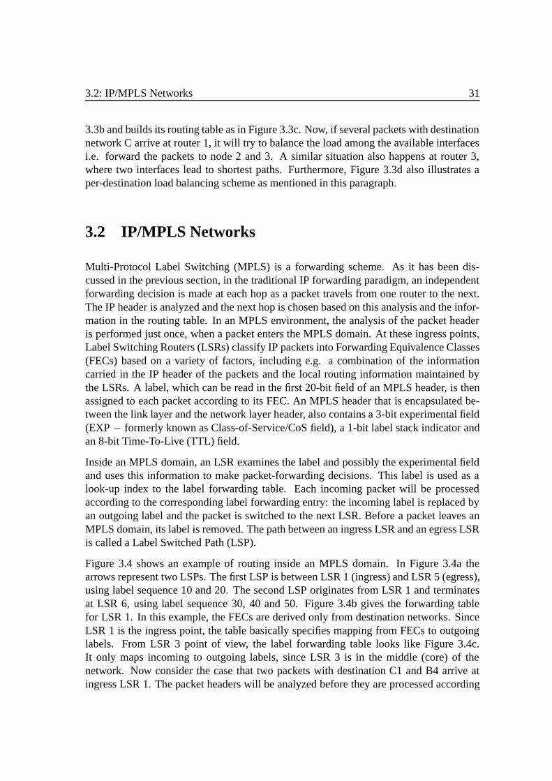
3.2: IP/MPLS Networks 31
3.3b and builds its routing table as in Figure 3.3c. Now, if several packets with destinationnetwork C arrive at router 1, it will try to balance the load among the available interfacesi.e. forward the packets to node 2 and 3. A similar situation also happens at router 3,where two interfaces lead to shortest paths. Furthermore, Figure 3.3d also illustrates aper-destination load balancing scheme as mentioned in this paragraph.
3.2 IP/MPLS Networks
Multi-Protocol Label Switching (MPLS) is a forwarding scheme. As it has been dis-cussed in the previous section, in the traditional IP forwarding paradigm, an independentforwarding decision is made at each hop as a packet travels from one router to the next.The IP header is analyzed and the next hop is chosen based on this analysis and the infor-mation in the routing table. In an MPLS environment, the analysis of the packet headeris performed just once, when a packet enters the MPLS domain. At these ingress points,Label Switching Routers (LSRs) classify IP packets into Forwarding Equivalence Classes(FECs) based on a variety of factors, including e.g. a combination of the informationcarried in the IP header of the packets and the local routing information maintained bythe LSRs. A label, which can be read in the first 20-bit field of an MPLS header, is thenassigned to each packet according to its FEC. An MPLS header that is encapsulated be-tween the link layer and the network layer header, also contains a 3-bit experimental field(EXP− formerly known as Class-of-Service/CoS field), a 1-bit label stack indicator andan 8-bit Time-To-Live (TTL) field.
Inside an MPLS domain, an LSR examines the label and possibly the experimental fieldand uses this information to make packet-forwarding decisions. This label is used as alook-up index to the label forwarding table. Each incoming packet will be processedaccording to the corresponding label forwarding entry: the incoming label is replaced byan outgoing label and the packet is switched to the next LSR. Before a packet leaves anMPLS domain, its label is removed. The path between an ingress LSR and an egress LSRis called a Label Switched Path (LSP).
Figure 3.4 shows an example of routing inside an MPLS domain. In Figure 3.4a thearrows represent two LSPs. The first LSP is between LSR 1 (ingress) and LSR 5 (egress),using label sequence 10 and 20. The second LSP originates from LSR 1 and terminatesat LSR 6, using label sequence 30, 40 and 50. Figure 3.4b gives the forwarding tablefor LSR 1. In this example, the FECs are derived only from destination networks. SinceLSR 1 is the ingress point, the table basically specifies mapping from FECs to outgoinglabels. From LSR 3 point of view, the label forwarding table looks like Figure 3.4c.It only maps incoming to outgoing labels, since LSR 3 is in the middle (core) of thenetwork. Now consider the case that two packets with destination C1 and B4 arrive atingress LSR 1. The packet headers will be analyzed before they are processed according
32 Chapter 3: Overview of IP Routing
Dest. LabelInter−faceLabel
Inter−face
In Out
LabelInter−faceLabel
Inter−face
In Out
1−A −
1−3
1−3
30
1 2
4
5
C
B
1 2
43
5 6
network A
network B network C
(a) (b)
(c)
10
20
30
40
50
6
3
(d)
3−5
3−4
30
10
20
1−3
1−3
20
40
40
50
10
B4
B4
B4C1
C1
C1
C1
B4
C1
30
10
1−A −
Figure 3.4: Routing with MPLS
to the forwarding table: (i) label 10 is inserted to packet B4, which is then forwarded toLSR 3; (ii) label 30 is imposed to packet C1, which is also forwarded to LSR 3. At LSR3, these packets are switched: incoming packet with label 10 is forwarded to LSR 5 withoutgoing label 20, while that with label 30 is forwarded to LSR 4 with outgoing label40. At the egress LSRs 5 and 6, the labels are removed and the packets are sent to thedestination hosts.
As inherently indicated in the previous example, An LSP is uni-directional from senderto receiver. LSPs can be set up either manually or signaled using protocols for labeldistribution. In the first case, one has to manually assign labels on all LSRs (ingress,transit and egress). In the second case, a signaling protocol is used to set up the path anddynamically assign labels. One just needs to configure the ingress routers, since transitand egress routers accept signaling information from the ingress router and they set upand maintain the LSP cooperatively. In both cases, the issue which intermediate LSRsan LSP may traverse is a management concern to be settled during a planning or a path

3.3: Differentiated Services 33
computation phase. The ability to set up Explicit Routes (ERs) for the LSPs is one of themost useful features of MPLS, since it provides a complete control over a routing path.This has not been easy to implement in the classical IP routing technology. For the lattercase, it is also possible to set up LSPs automatically:
• by using (vanilla) Label Distribution Protocol (LDP). The LSPs established by theLDP are identical to the routing paths yielded by hop-by-hop IP routing. LDPbasically maps network layer routing information from IGP directly to MPLS layer.Two LSPs as depicted in Figure 3.4a could be generated by LDP for the weightsystem as shown in Figure 3.2a.
• by using either Constraint-based Routing Label Distribution Protocol (CR-LDP)or Resource reSerVation Protocol with Traffic Engineering extension (RSVP-TE).These protocols perform Constraint-Based Routing (CBR)8 to automatically com-pute the intermediate hops of an LSP. LSP setup can be control driven i.e. triggeredby control traffic such as routing updates. Or, it can be data driven i.e. triggered bythe request of a flow or an aggregation of flows [XN99].
3.3 Differentiated Services
There are two architectures for adding QoS capabilities to today’s IP networks: IntegratedServices (IntServ) and Differentiated Services (DiffServ/DS). IntServ maintains an end-to-end QoS for an individual or a group of flows with the help of a signaling protocolsuch as RSVP. The idea behind IntServ is that routers have to be able to reserve resourcesin order to provide QoS for specific user packet streams or flows. This unfortunatelyrequiresflow-specific9 state to be maintained in the routers, which in turn makes IntServlacking scalability, since the amount of state information increases proportionally withthe number of flows. DiffServ, on the other hand, works on the provisioned-QoS modelwhere network elements are set up to service multiple classes of traffic, with varyingrequirements. Its basic idea is to keep packet forwarding simple by categorizing trafficinto (a small numberof) different classes and thus removing flow-specific informationfrom the network core. Therefore, DiffServ is the preferred technology for large-scale IPQoS deployments [FE02].
Traffic entering a DS-domain is classified, policed and possibly conditioned at the edgesof the network, and assigned to different Behaviour Aggregates (BAs). Each behaviour
8CBR denotes a class of routing algorithms that base path selection decisions on a set of requirementsor constraints, in addition to destination.
9Here, the definition offlow is more general than that as given in Chapter 2. For example, packets withthe same value of (src. address; src. port; dest. address; dest. port) might be considered as a flow.

34 Chapter 3: Overview of IP Routing
LabelInter−faceLabel
Inter−face
In Out
Class
FEC
Dest.
LabelInter−faceLabel
Inter−face
In Out
network A
30 6040
C
C
60
70
(a)
4−6
4−6
80
network C
50
4−3
4−2
80
50
LSP 1
LSP 2
(b)
(c)
40
70
1
1−2
1−3
2
−
−43
1−A
1−A 30
5 6
P
BE
Figure 3.5: Class-based routing in a DS-MPLS network
aggregate is identified by a single Differentiated Services Code Point (DSCP), which is lo-cated at the first six bits in the DS-field10 of the IP header. Within the core of the network,scheduling and queueing control mechanisms are applied to the traffic classes accord-ing to the Per-Hop Behaviour (PHB) associated with the DSCP. By assigning traffic ofdifferent classes to different DSCPs, the DiffServ network provides different forwardingtreatements and thus different levels of QoS. Currently, several PHBs are defined:
• The Expedited Forwarding (EF) PHB. The EF PHB is used to provide premiumservices i.e. for traffic with low loss, low delay, low jitter, assured bandwidth re-quirements, such as Voice over IP (VoIP), video or online trading software.
• The Assured Forwarding (AF) PHB. The AF PHB is used to support data trafficwith assured bandwidth requirements. It is further divided into four subclasses.Within each subclass it is possible to specify 3 drop precedence values. This PHBcan be used to provide olympic services (i.e. three tiers of services: gold, silver andbronze, with decreasing quality).
• The Default (DF) PHB. The DF PHB represents the default forwarding behaviour.Packets, which are not identified as belonging to another class, belong to this ag-gregate. This PHB is typically used for the classical best effort services.
DiffServ can be deployed together with MPLS. In this so-called DS-MPLS architecture,packets marked with DSCP will enter the MPLS network and PHB is enforced by every
10The DS-field replaces the original ToS byte in IPv4 (IP version 4) or theTraffic Classfield in IPv6.
3.3: Differentiated Services 35
LSR along the path. As LSRs do not have any knowledge of the IP header, PHB hasto be achieved by looking at different information. Two general approaches are used tomark MPLS traffic for QoS handling within an MPLS network [DR00, CIS]. In the firstmethod, the DS coloring information is mapped in the EXP field of the MPLS header.LSPs that use this approach are called E-LSPs, where packets are buffered and sched-uled in accordance with the EXP fields. Alternatively, the label associated with eachMPLS packet carries the portion of the DS marking that specifies how a packet should bequeued. The dropping precedence portion of the DS marking is carried in the EXP bits.The ingress LSR examines the DSCP in the IP header and selects an LSP that has beenprovisioned for that QoS level. LSPs using this approach are called L-LSPs where QoSinformation is inferred from the MPLS label.
It is obvious that routing by means of E-LSPs can happen both atclassor coarser granu-larity, while that using L-LSPs can only occur at class granularity. Since in our context,we considerclass-based routing, it does not really matter which type of LSP is used. Thischapter will be closed with an example of a class-based routing mechanism inside a DS-MPLS network as described in Figure 3.5, which is, to a great extent, self explanatory.Consider that we have two classes of traffic to be routed from LSR 1 to LSR 6: premiumtraffic (denoted by P) and best effort traffic (BE). This means that two LSPs (one for eachclass) has to be established. These are, for example, configured as in Figure 3.5a. Assumethat LSP 1 is allocated for premium and LSP 2 for best effort traffic. At ingress LSR 1 thelabel forwarding table has to be set appropriately i.e. class information has to be includedin the FECs. Such a label forwarding table is given in Figure 3.5b. Actually, this is theonly difference between DS and non DS-compliant MPLS networks, since in the core ofthe network, packets are switched in the same manner (cf. Figure 3.4c and Figure 3.5c).Note that for the case of E-LSPs, LSPs 1 and 2 could use the same label at link (4,6), aslabels do not correspond to DSCP. By contrast, in the case of L-LSPs, two LSPs for twodifferent traffic classes can not share labels, even if the paths are identical.

36 Chapter 3: Overview of IP Routing
Chapter 4
Traffic Engineering in Classical andTransitional IP Networks
To cope with the rapid growth of the Internet and due to increasing requirements for ser-vice quality, some efforts have been invested by Internet Service Providers (ISPs), to builda more scalable network architecture and expand network infrastructure and capacity. An-other important issue is traffic engineering, that could give ISPs some degree of controlof the traffic distributed over the network. In routing context, traffic engineering meansmapping traffic flows onto the existing physical network topology in the most effectiveway to accomplish desired operational objectives. This issue is the main focus of thischapter, which is organized as follows. First, in Section 4.1 we deal with traffic engi-neering problem in classical IP networks. After that, in Section 4.2 we consider severaltypes of transitional IP networks and propose the corresponding traffic engineering solu-tion. Further, Section 4.3 addresses the issue of partial demand increase and its impact onresource occupancy. Finally, some general remarks and other traffic engineering relatedactivities are given in Section 4.4.
4.1 Metric-Based Traffic Engineering
The Internet was designed as abest effortnetwork and was not designed to guarantee aparticular level of performance, certainly not end-to-end quality of service [Gou01]. Inthis regard, traffic engineering can be viewed as a part of efforts to improve the capabil-ity of IP networks to provide better services. InclassicalIP networks, there are severalapproaches for deploying traffic engineering: by optimizing the parameters used for rout-ing decisions, so that a better network performance will be obtained [FT00] [SKK00][Gou01] [MK02b] [KP00] [BAGLM00], or by using explicit routing in an overlay modelwith ATM or Frame Relay technology [WWZ01]. Recent developments in MPLS open
37
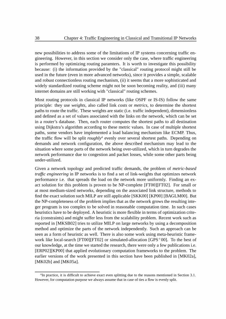
38 Chapter 4: Traffic Engineering in Classical and Transitional IP Networks
new possibilities to address some of the limitations of IP systems concerning traffic en-gineering. However, in this section we consider only the case, where traffic engineeringis performed by optimizing routing paramters. It is worth to investigate this possibilitybecause: (i) the information provided by the "classical" routing protocol might still beused in the future (even in more advanced networks), since it provides a simple, scalableand robust connectionless routing mechanism, (ii) it seems that a more sophisticated andwidely standardized routing scheme might not be soon becoming reality, and (iii) manyinternet domains are still working with "classical" routing schemes.
Most routing protocols in classical IP networks (like OSPF or IS-IS) follow the sameprinciple: they useweights, also called linkcostsor metrics, to determine the shortestpaths to route the traffic. These weights are static (i.e. traffic independent), dimensionlessand defined as a set of values associated with the links on the network, which can be setin a router’s database. Then, each router computes the shortest paths to all destinationusing Dijkstra’s algorithm according to these metric values. In case of multiple shortestpaths, some vendors have implemented a load balancing mechanism like ECMP. Thus,the traffic flow will be splitroughlya evenly over several shortest paths. Depending ondemands and network configuration, the above described mechanism may lead to thesituation where some parts of the network being over-utilized, which in turn degrades thenetwork performance due to congestion and packet losses, while some other parts beingunder-utilized.
Given a network topology and predicted traffic demands, the problem ofmetric-basedtraffic engineeringin IP networks is to find a set of link-weights that optimizes networkperformance i.e. that spreads the load on the network more uniformly. Finding an ex-act solution for this problem is proven to be NP-complete [FT00][FT02]. For small orat most medium-sized networks, depending on the associated link structure, methods tofind the exact solution such MILP are still applicable [SKK00] [KP00] [BAGLM00]. Butthe NP-completeness of the problem implies that as the network grows the resulting inte-ger program is too complex to be solved in reasonable computation time. In such casesheuristics have to be deployed. A heuristic is more flexible in terms of optimization crite-ria (constraints) and might suffer less from the scalability problem. Recent work such asreported in [MKSB02] tries to utilize MILP on large networks by using a decompositionmethod and optimize the parts of the network independently. Such an approach can beseen as a form of heuristic as well. There is also some work using meta-heuristic frame-work like local-search [FT00][FT02] or simulated-allocation [GPS+00]. To the best ofour knowledge, at the time we started the research, there were only a few publications i.e.[ERP02][KP00] that applied evolutionary computation frameworks to the problem. Theearlier versions of the work presented in this section have been published in [MK02a],[MK02b] and [MK05a].
aIn practice, it is difficult to achieve exact even splitting due to the reasons mentioned in Section 3.1.However, for computation purpose we always assume that in case of ties a flow is evenly split.
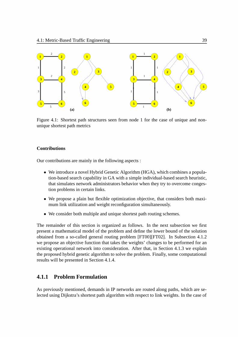
4.1: Metric-Based Traffic Engineering 39
(b)(a)
6
11
1
1
1
1
2
21
2
3
5
5
121
3 4
5 6
2
3 4
5 6
1
2
4
6
5
3
1
2 3
4 5
1
Figure 4.1: Shortest path structures seen from node 1 for the case of unique and non-unique shortest path metrics
Contributions
Our contributions are mainly in the following aspects :
• We introduce a novel Hybrid Genetic Algorithm (HGA), which combines a popula-tion-based search capability in GA with a simple individual-based search heuristic,that simulates network administrators behavior when they try to overcome conges-tion problems in certain links.
• We propose a plain but flexible optimization objective, that considers both maxi-mum link utilization and weight reconfiguration simultaneously.
• We consider both multiple and unique shortest path routing schemes.
The remainder of this section is organized as follows. In the next subsection we firstpresent a mathematical model of the problem and define the lower bound of the solutionobtained from a so-called general routing problem [FT00][FT02]. In Subsection 4.1.2we propose an objective function that takes the weights’ changes to be performed for anexisting operational network into consideration. After that, in Section 4.1.3 we explainthe proposed hybrid genetic algorithm to solve the problem. Finally, some computationalresults will be presented in Section 4.1.4.
4.1.1 Problem Formulation
As previously mentioned, demands in IP networks are routed along paths, which are se-lected using Dijkstra’s shortest path algorithm with respect to link weights. In the case of
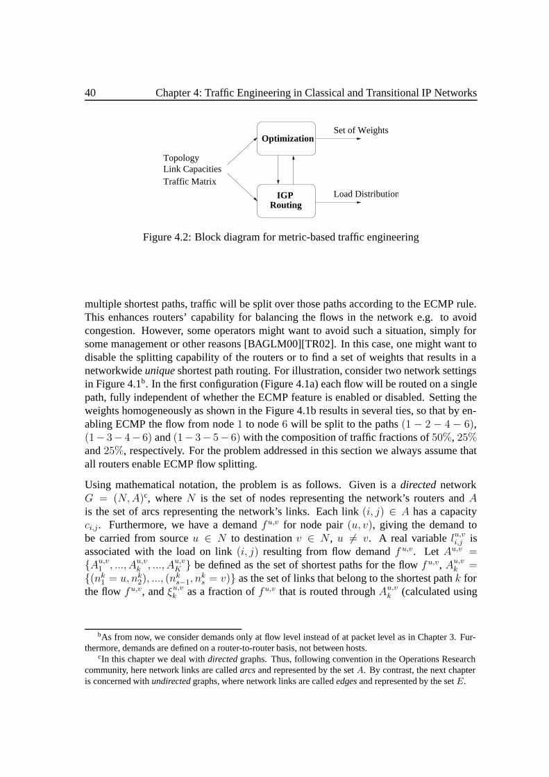
40 Chapter 4: Traffic Engineering in Classical and Transitional IP Networks
IGP
Link CapacitiesTraffic Matrix
Optimization
Routing
Set of Weights
Load Distribution
Topology
Figure 4.2: Block diagram for metric-based traffic engineering
multiple shortest paths, traffic will be split over those paths according to the ECMP rule.This enhances routers’ capability for balancing the flows in the network e.g. to avoidcongestion. However, some operators might want to avoid such a situation, simply forsome management or other reasons [BAGLM00][TR02]. In this case, one might want todisable the splitting capability of the routers or to find a set of weights that results in anetworkwideuniqueshortest path routing. For illustration, consider two network settingsin Figure 4.1b. In the first configuration (Figure 4.1a) each flow will be routed on a singlepath, fully independent of whether the ECMP feature is enabled or disabled. Setting theweights homogeneously as shown in the Figure 4.1b results in several ties, so that by en-abling ECMP the flow from node1 to node6 will be split to the paths(1 − 2 − 4 − 6),(1− 3− 4− 6) and(1− 3− 5− 6) with the composition of traffic fractions of50%, 25%and25%, respectively. For the problem addressed in this section we always assume thatall routers enable ECMP flow splitting.
Using mathematical notation, the problem is as follows. Given is adirectednetworkG = (N,A)c, whereN is the set of nodes representing the network’s routers andAis the set of arcs representing the network’s links. Each link(i, j) ∈ A has a capacityci,j. Furthermore, we have a demandfu,v for node pair(u, v), giving the demand tobe carried from sourceu ∈ N to destinationv ∈ N , u = v. A real variablelu,vi,j isassociated with the load on link(i, j) resulting from flow demandf u,v. Let Au,v =Au,v1 , ..., Au,vk , ..., Au,vK be defined as the set of shortest paths for the flowf u,v, Au,vk =(nk1 = u, nk2), ..., (n
ks−1, n
ks = v) as the set of links that belong to the shortest pathk for
the flowfu,v, andξu,vk as a fraction offu,v that is routed throughAu,vk (calculated using
bAs from now, we consider demands only at flow level instead of at packet level as in Chapter 3. Fur-thermore, demands are defined on a router-to-router basis, not between hosts.
cIn this chapter we deal withdirectedgraphs. Thus, following convention in the Operations Researchcommunity, here network links are calledarcsand represented by the setA. By contrast, the next chapteris concerned withundirectedgraphs, where network links are callededgesand represented by the setE.

4.1: Metric-Based Traffic Engineering 41
the ECMP rule). The total load on the link(i, j) can be computed as follows:
li,j =∑uv
lu,vi,j =∑uv
fu,v · βu,vi,j (4.1)
where
βu,vi,j =∑k
∑l∈Au,v
k
δli,j · ξu,vk (4.2)
δli,j =
1 if l = (i, j)
0 otherwise(4.3)
∑k
ξu,vk = 1 (4.4)
Note that in the case ofuniqueshortest path routing i.e.K = 1, (4.2) becomesβu,vi,j =∑l∈Au,v
1δli,j. The block diagram for metric based traffic engineering is depicted in Figure
4.2. For a given capacitated network and the corresponding traffic matrixF = (f u,v), u =v ∈ N , the problem is to find a set of metrics (a weight system)W = (wi,j), ∀(i, j) ∈ Ato increase the network performance which can be formulated as :
min c1 · ρmax + φ (4.5)
ρi,j ≤ ρmax;∀(i, j) ∈ A (4.6)
whereρi,j =li,jci,j
is the utilization of the link(i, j). With (4.5) we prefer solutions witha low ρmax, which implies that the network is better utilized. The second termφ couldbe used for accomodating different objectives (e.g. weight reconfiguration), whilst theconstantc1 will be used for trading between these two components. Using the simpleobjectiveρmax in some cases may need special treatment. In a network, where there areno possibilities to reroute traffic traversing a subset of links, it would be better to excludethem for computingρmax in (4.6)d.
Since here we do not have any explicit mathematical relationships betweenξu,vk (con-tained inρi,j) and decision variablewi,j, the formulation (4.5)−(4.6) can not be solvedusing mathematical programming approachese. It is intended for the heuristic solving
dAn example of such a network topology will be presented in Section 4.2 and discussed in Subsection4.2.3.
eDifficulty for obtaining such a mathematical relationship is mainly due to the ECMP rule: if it is notconsidered, the problem of metric-based traffic engineering can be formulated as a linear program (cf.[SKK00])

42 Chapter 4: Traffic Engineering in Classical and Transitional IP Networks
method as will be addressed in Subsection 4.1.3. Having the traffic matrix and a weightsystemf, we can compute the load distribution on the network. Every solution has a qualitymeasure according to (4.5). Although a solution is feasible ifρi,j ≤ 1 or correspondinglyρmax ≤ 1, the optimization is performed with no constraints to force this condition, butwe simply minimize the objective function. The desired result then is a set of weightswhich corresponds to the minimized cost function. Of course valuable results are onlythose which would keep the utilization level below1 for all links of the network.
General Routing Problem (GRP)
To valuate routing solutions given by our heuristic approach, we can make a comparisonwith a so-called general routing problem [FT00] [FT02] as a lower bound. In this generalrouting problem, there are no limitations on how flows can be distributed along the pathsfrom source to destination, and the problem can be formulated and solved in polynomialtime as a multi commodity flow problem without integrality constraints. The generalrouting problem optimization can be formulated as follows:
min
c1 · ρmax +
1
|A|∑ij
∑uv
fu,vxu,vi,jci,j
(4.7)
∑uv
fu,vxu,vi,jci,j
≤ ρmax ; ∀(i, j) ∈ A (4.8)
δu,n +∑
∀(m,n)∈Axu,vm,n = δn,v +
∑∀(n,m)∈A
xu,vn,m ; ∀fu,v, ∀n ∈ N (4.9)
0 ≤ xu,vi,j ≤ 1 ; ∀fu,v , ∀(i, j) ∈ A (4.10)
(4.7) is the objective function to minimizeρmax and the average utilizationρ = 1|A|∑
ij ρi,j,
whereρi,j =∑
uv
fu,vxu,vi,j
ci,j, ∀(i, j) ∈ A. The second termρ in (4.7) is necessary to avoid
routing loops (for the optimal solutiong). Since the objective functions in (4.5) could takea form different from (4.7), which will be discussed in the next subsection, the result fromGRP theoretically is not the lower bound for our problem. But by choosing a quite highvalue ofc1 in both equations, we can be quite confident that GRP will provide a lowerbound. The variablexu,vi,j is associated with the fraction off u,v that flows on the link(i, j). (4.9) describes flow conservation constraints that ensure the desired traffic flow tobe routed from source to destination. The Kronecker deltaδi,j is defined as having thevalue one wheni = j and zero wheni = j.
f If it is provided by the heuristic as a temporary solution, for instance.gBecause there are no loop-avoidance constraints, a solution which contains routing loops is also valid.
But the value ofρ of such a solution is definitely worse than that without loops.
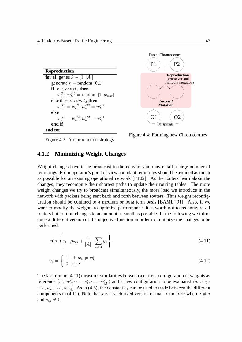
4.1: Metric-Based Traffic Engineering 43
Reproductionfor all genesk ∈ [1, |A|]
generater = random [0,1]if r < const1 thenwO1k , wO2
k = random[1, wmax]else if r < const2 thenwO1k = wP1
k , wO2k = wP2
k
elsewO1k = wP2
k , wO2k = wP1
k
end ifend for
Figure 4.3: A reproduction strategy
Parent Chromosomes
Offsprings
Reproduction(crossover andrandom mutation)
TargetedMutation
O2
P1 P2
O1
Figure 4.4: Forming new Chromosomes
4.1.2 Minimizing Weight Changes
Weight changes have to be broadcast in the network and may entail a large number ofreroutings. From operator’s point of view abundant reroutings should be avoided as muchas possible for an existing operational network [FT02]. As the routers learn about thechanges, they recompute their shortest paths to update their routing tables. The moreweight changes we try to broadcast simultaneously, the more load we introduce in thenetwork with packets being sent back and forth between routers. Thus weight reconfig-uration should be confined to a medium or long term basis [BAML+01]. Also, if wewant to modify the weights to optimize performance, it is worth not to reconfigure allrouters but to limit changes to an amount as small as possible. In the following we intro-duce a different version of the objective function in order to minimize the changes to beperformed.
min
c1 · ρmax +
1
|A| ·∑k∈A
yk
(4.11)
yk =
1 if wk = wrk0 else
(4.12)
The last term in (4.11) measures similarities between a current configuration of weights asreference〈wr1, wr2, · · · , wrk, · · · , wr|A|〉 and a new configuration to be evaluated〈w1, w2,-· · · , wk, · · · , w|A|〉. As in (4.5), the constantc1 can be used to trade between the differentcomponents in (4.11). Note thatk is a vectorized version of matrix indexij wherei = jandci,j = 0.
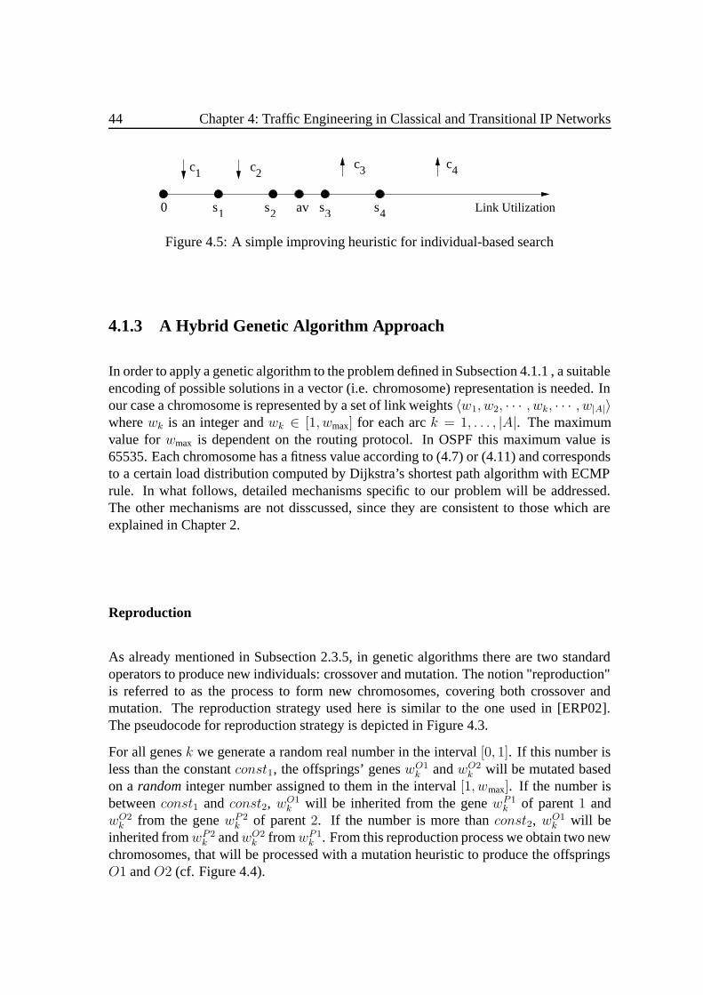
44 Chapter 4: Traffic Engineering in Classical and Transitional IP Networks
Link Utilization
c2c3c1
c4
av0 s1 s2 s3 s4
Figure 4.5: A simple improving heuristic for individual-based search
4.1.3 A Hybrid Genetic Algorithm Approach
In order to apply a genetic algorithm to the problem defined in Subsection 4.1.1 , a suitableencoding of possible solutions in a vector (i.e. chromosome) representation is needed. Inour case a chromosome is represented by a set of link weights〈w1, w2, · · · , wk, · · · , w|A|〉wherewk is an integer andwk ∈ [1, wmax] for each arck = 1, . . . , |A|. The maximumvalue forwmax is dependent on the routing protocol. In OSPF this maximum value is65535. Each chromosome has a fitness value according to (4.7) or (4.11) and correspondsto a certain load distribution computed by Dijkstra’s shortest path algorithm with ECMPrule. In what follows, detailed mechanisms specific to our problem will be addressed.The other mechanisms are not disscussed, since they are consistent to those which areexplained in Chapter 2.
Reproduction
As already mentioned in Subsection 2.3.5, in genetic algorithms there are two standardoperators to produce new individuals: crossover and mutation. The notion "reproduction"is referred to as the process to form new chromosomes, covering both crossover andmutation. The reproduction strategy used here is similar to the one used in [ERP02].The pseudocode for reproduction strategy is depicted in Figure 4.3.
For all genesk we generate a random real number in the interval[0, 1]. If this number isless than the constantconst1, the offsprings’ geneswO1
k andwO2k will be mutated based
on arandominteger number assigned to them in the interval[1, wmax]. If the number isbetweenconst1 and const2, wO1
k will be inherited from the genewP1k of parent1 and
wO2k from the genewP2
k of parent2. If the number is more thanconst2, wO1k will be
inherited fromwP2k andwO2
k fromwP1k . From this reproduction process we obtain two new
chromosomes, that will be processed with a mutation heuristic to produce the offspringsO1 andO2 (cf. Figure 4.4).

4.1: Metric-Based Traffic Engineering 45
fail=fail+1
B betterthan C ?
C=Bfail=0
?(fail<threshold)
yes
no
yes
noChr. C
Chr. B
Apply heuristicto C
C=AChr. A
Figure 4.6: The individual-based search
Targeted Mutation and Individual-based Search
In addition to the reproduction process one type of mutation is additionally implemented.We apply a heuristic to mutate some genes from offsprings resulting from the reproduc-tion process. We simply add (substract) a random number to the weightwk if the linkutilization from an arck is bigger (lower) than a particular treshold because we know thatthe bigger the weight, the lower the chance that traffic will get routed on that link andvice versa. This approach can be seen as a simple improving heuristic as mentioned inSubsection 2.3.6, which simulates network administrators behavior when they try to over-come congestion problems or just, to reroute parts of the traffic on a certain link. Withthis type of mutation we hope, that the offspringsO1 andO2 have a better link utilizationat k, and hopefully also a better fitness value. This can be seen as a "targeted" mutationproposed for other problems in [Bec01]. Figure 4.5 shows an example of this heuristicin more detail. If the current link utilization is larger thans4, we increase the link costfor that arc by a factorc4. If the current link utilization is lower thans1, we decreasethe link cost for that arc by a factorc1 etc. The constantsci are actually implemented asupper bounds for these weight changes i.e. the actual constants are randomly generatedwith theseci as upper bounds. Therefore the influence of the targeted mutation is still ofstochastic nature.
The same heuristic is also used to perform individual-based search inside the genetic al-gorithm, forming a hybrid approach as mentioned in Subsection 2.3.6. The populationdynamics are similar to those in Figure 2.14 by replacing the block PLS with the block"heuristic search" as displayed in Figure 4.6h. It basically works as follows. A chromo-
hFor clarity, the reason why the term "heuristic search" is used instead of "PLS" is, that here we do notdefine systematic neighborhood criteria. In other words, we always accept a better solution given by theheuristic regardless its structure.
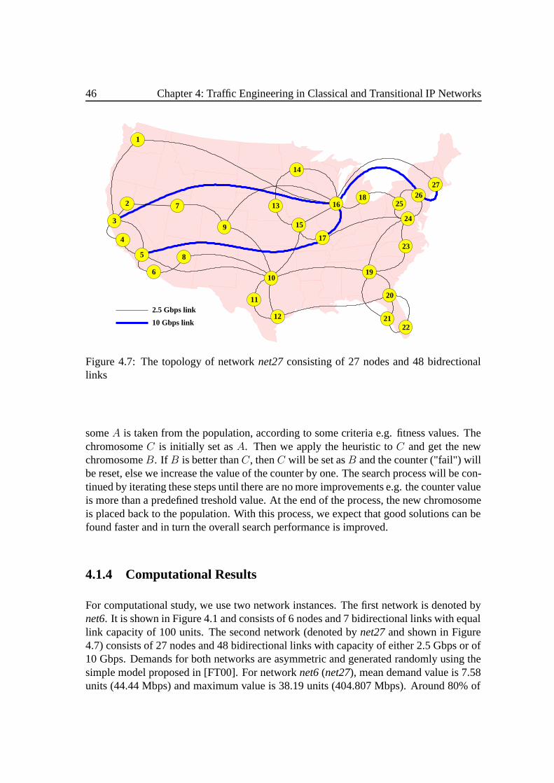
46 Chapter 4: Traffic Engineering in Classical and Transitional IP Networks
10 Gbps link
1
3
4
7
9
5
6
8
10
11
12
13
14
15
17
18
19
20
2122
23
24
2526
27
16
2.5 Gbps link
2
Figure 4.7: The topology of networknet27consisting of 27 nodes and 48 bidrectionallinks
someA is taken from the population, according to some criteria e.g. fitness values. ThechromosomeC is initially set asA. Then we apply the heuristic toC and get the newchromosomeB. If B is better thanC, thenC will be set asB and the counter ("fail") willbe reset, else we increase the value of the counter by one. The search process will be con-tinued by iterating these steps until there are no more improvements e.g. the counter valueis more than a predefined treshold value. At the end of the process, the new chromosomeis placed back to the population. With this process, we expect that good solutions can befound faster and in turn the overall search performance is improved.
4.1.4 Computational Results
For computational study, we use two network instances. The first network is denoted bynet6. It is shown in Figure 4.1 and consists of 6 nodes and 7 bidirectional links with equallink capacity of 100 units. The second network (denoted bynet27and shown in Figure4.7) consists of 27 nodes and 48 bidirectional links with capacity of either 2.5 Gbps or of10 Gbps. Demands for both networks are asymmetric and generated randomly using thesimple model proposed in [FT00]. For networknet6(net27), mean demand value is 7.58units (44.44 Mbps) and maximum value is 38.19 units (404.807 Mbps). Around 80% of

4.1: Metric-Based Traffic Engineering 47
1 2 3 4 5 6 7 8 9 10 11 12 13 140
0.2
0.4
0.6
0.8
1Initial Utilization
Util
izat
ion
Link number (directed)1 2 3 4 5 6 7 8 9 10 11 12 13 14
0
0.2
0.4
0.6
0.8
1Optimized Utilization
Util
izat
ion
Link number (directed)
Figure 4.8: Link utilization of networknet6before and after optimization
the demands are below 12 units (66 Mbps).
Utilization and Weight Changes
Figure 4.8 shows link utilization before and after optimization fornet6. Initially, linkweight was set homogeneously to the value of 10. Thus, with this setting, 12 flows willbe split i.e. the flows between nodes (1,4),(1,6),(2,3),(2,5),(3,6) and (4,5). This resultsin maximum utilization of 0.893 and average utilization of 0.271 (Figure 4.8 left). Afteroptimization we obtain a better distribution as shown in Figure 4.8 right, with maximumutilization of 0.541. This result has been achieved by 42.9% weight changes i.e. changingthe weight for: links (1,2) to the value of 2, link (1,3) to the value of 7 and link (5,6) tothe value of 1. With this setting only two flows between nodes (2,6) will be split. Withrespect to the value of maximum utilization, this result is very close to the theoreticallower bound of 0.537 derived from GRP.
For the following discussion we use networknet27the link weights of which were origi-nally set inversely proportional to the link capacities.
Convergence
Figure 4.9 and Figure 4.10 show the convergence of average fitness in the population. Toexclude the influence of the start population, the values have been calculated as mean val-ues obtained from 10 independent runs. GA denotes a rather standard genetic algorithm,that uses the reproduction strategy from [ERP02] as discussed in Subsection 4.1.3. HGA

48 Chapter 4: Traffic Engineering in Classical and Transitional IP Networks
100
101
102
600
800
1000
1200
1400
1600
1800
Fitness Convergence (Average Population Fitness )
Fitn
ess
Iteration Number
LP lower bound
GA (mean values of 10 runs)
HGA (mean values of 10 runs)
Figure 4.9: The convergence characteristicof the HGA compared to a normal GA andthe LP lower bound foraveragepopulationfitness
100
101
102
600
800
1000
1200
1400
1600
1800
Fitness Convergence (Best Individual)
Fitn
ess
Iteration Number
GA (mean values of 10 runs)
HGA (mean values of 10 runs)
LP lower bound
Figure 4.10: The convergence characteris-tic of the HGA compared to a normal GAand the LP lower bound forbest individualfitness
denotes the result of our hybrid GA, that additionally performs individual-based heuris-tic search. As seen from the figures, HGA tends to converge faster than GA, but for ahigher number of iterations the performance shown by GA and HGA does not differ verymuch. Based on these results, since the additional modules performing individual searchcertainly take more time than the standard one, several tradeoffs could be made e.g. weapply HGA at the beginning and continue with the normal GA after a certain iterationnumber. We did not compare these two approaches with respect to computation time ina systematic way, but our experiments (for networknet27) show the computation timeneeded for HGA is about twice as high as that for the standard GA.
Increasing Traffic
Finally we present the results of our method for the case of increasing traffic demands.In Figures 4.11 and 4.12 we compare the maximum utilization based on some commonlyused metrics to our results and to a lower bound resulting from the linear programmingresult of the general routing problem. In Figure 4.11 we use (4.7) as objective function.In Figure 4.12 we used the second objective function (4.11). For comparison we consid-ered hop count metric (denoted byUnitOSPF) and inverse capacities metric (denoted byInvCapOSPF) which was also used as reference weight setting in Figure 4.12. HGA-X orHGA-X(Y%) denote the results for X iterations and Y% relative changes (to be applied tothe reference weight configuration) i.e. Y refers to the last term of (4.11). For both typesof calculation, the value ofwmax was set to 20. The figures show that in comparison with
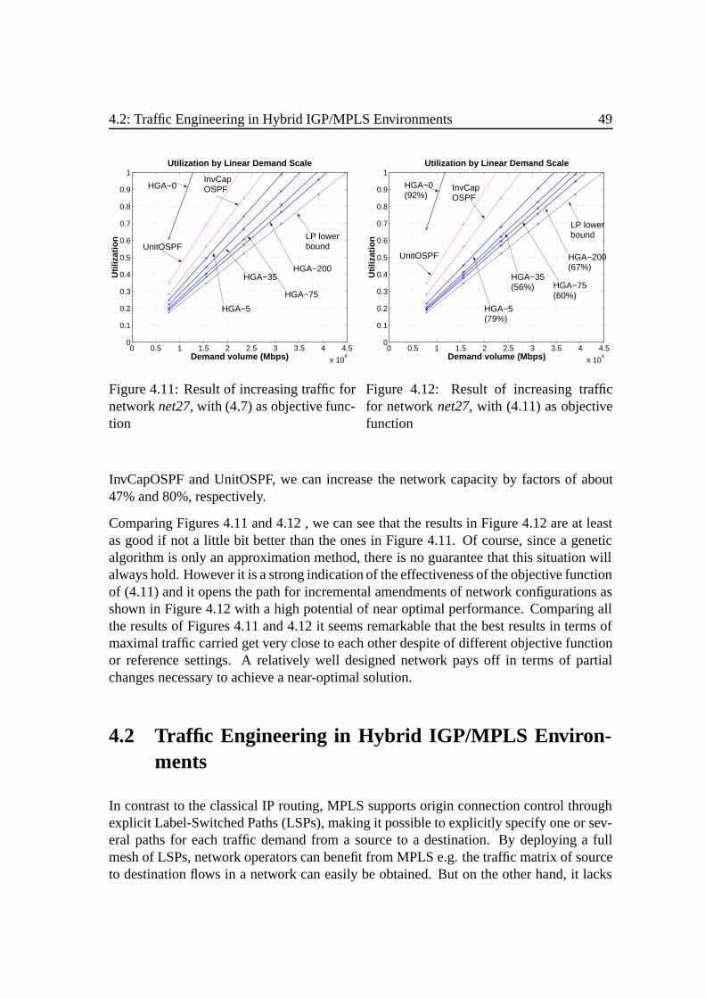
4.2: Traffic Engineering in Hybrid IGP/MPLS Environments 49
0 0.5 1 1.5 2 2.5 3 3.5 4 4.5
x 104
0
0.1
0.2
0.3
0.4
0.5
0.6
0.7
0.8
0.9
1Utilization by Linear Demand Scale
Util
izat
ion
Demand volume (Mbps)
HGA−0
UnitOSPF
InvCapOSPF
LP lowerbound
HGA−5
HGA−35
HGA−75
HGA−200
Figure 4.11: Result of increasing traffic fornetworknet27, with (4.7) as objective func-tion
0 0.5 1 1.5 2 2.5 3 3.5 4 4.5
x 104
0
0.1
0.2
0.3
0.4
0.5
0.6
0.7
0.8
0.9
1Utilization by Linear Demand Scale
Util
izat
ion
Demand volume (Mbps)
HGA−0 (92%)
UnitOSPF
InvCapOSPF
LP lowerbound
HGA−5 (79%)
HGA−35(56%) HGA−75
(60%)
HGA−200(67%)
Figure 4.12: Result of increasing trafficfor networknet27, with (4.11) as objectivefunction
InvCapOSPF and UnitOSPF, we can increase the network capacity by factors of about47% and 80%, respectively.
Comparing Figures 4.11 and 4.12 , we can see that the results in Figure 4.12 are at leastas good if not a little bit better than the ones in Figure 4.11. Of course, since a geneticalgorithm is only an approximation method, there is no guarantee that this situation willalways hold. However it is a strong indication of the effectiveness of the objective functionof (4.11) and it opens the path for incremental amendments of network configurations asshown in Figure 4.12 with a high potential of near optimal performance. Comparing allthe results of Figures 4.11 and 4.12 it seems remarkable that the best results in terms ofmaximal traffic carried get very close to each other despite of different objective functionor reference settings. A relatively well designed network pays off in terms of partialchanges necessary to achieve a near-optimal solution.
4.2 Traffic Engineering in Hybrid IGP/MPLS Environ-ments
In contrast to the classical IP routing, MPLS supports origin connection control throughexplicit Label-Switched Paths (LSPs), making it possible to explicitly specify one or sev-eral paths for each traffic demand from a source to a destination. By deploying a fullmesh of LSPs, network operators can benefit from MPLS e.g. the traffic matrix of sourceto destination flows in a network can easily be obtained. But on the other hand, it lacks
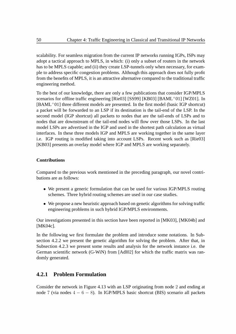
50 Chapter 4: Traffic Engineering in Classical and Transitional IP Networks
scalability. For seamless migration from the current IP networks running IGPs, ISPs mayadopt a tactical approach to MPLS, in which: (i) only a subset of routers in the networkhas to be MPLS capable; and (ii) they create LSP-tunnels only when necessary, for exam-ple to address specific congestion problems. Although this approach does not fully profitfrom the benefits of MPLS, it is an attractive alternative compared to the traditional trafficengineering method.
To the best of our knowledge, there are only a few publications that consider IGP/MPLSscenarios for offline traffic engineering [Rie03] [SS99] [KB03] [BAML+01] [WZ01]. In[BAML +01] three different models are presented. In the first model (basic IGP shortcut)a packet will be forwarded to an LSP if its destination is the tail-end of the LSP. In thesecond model (IGP shortcut) all packets to nodes that are the tail-ends of LSPs and tonodes that are downstream of the tail-end nodes will flow over those LSPs. In the lastmodel LSPs are advertised in the IGP and used in the shortest path calculation as virtualinterfaces. In these three models IGP and MPLS are working together in the same layeri.e. IGP routing is modified taking into account LSPs. Recent work such as [Rie03][KB03] presents an overlay model where IGP and MPLS are working separately.
Contributions
Compared to the previous work mentioned in the preceding paragraph, our novel contri-butions are as follows:
• We present a generic formulation that can be used for various IGP/MPLS routingschemes. Three hybrid routing schemes are used in our case studies.
• We propose a new heuristic approach based on genetic algorithms for solving trafficengineering problems in such hybrid IGP/MPLS environments.
Our investigations presented in this section have been reported in [MK03], [MK04b] and[MK04c].
In the following we first formulate the problem and introduce some notations. In Sub-section 4.2.2 we present the genetic algorithm for solving the problem. After that, inSubsection 4.2.3 we present some results and analysis for the network instance i.e. theGerman scientific network (G-WiN) from [Adl02] for which the traffic matrix was ran-domly generated.
4.2.1 Problem Formulation
Consider the network in Figure 4.13 with an LSP originating from node2 and ending atnode7 (via nodes4 − 6 − 8). In IGP/MPLS basic shortcut (BIS) scenario all packets

4.2: Traffic Engineering in Hybrid IGP/MPLS Environments 51
3
(c)
82
1
7
LSP
31
15 6
42
1 2
21
1
1
1
998
6 7
4 5
2 3
1
LSP
1
2 3
4 5
6 7
LSP
8 9
4
1
2 3
5
6 7
LSP
8 9
(a) (b)
2
Figure 4.13: Shortest path trees for the three different scenarios : Basic IGP shortcut, IGPshortcut and Overlay
arriving in node2 with destination of node7, will be forwarded to the LSP. Figure 4.13ashows the shortest path tree for node1. It is obvious that in the BIS model only the node7 is reachable via the LSP, while the other flows will follow the normal path. In the IGPshortcut (IS) scenario all packets arriving in node2 with destination of node7 as wellas of its downstreams i.e. the nodes8 and9 will be forwarded to the LSP. Figure 4.13bshows the shortest path tree in the IS model. Note that the link(5, 7) will not be usedfor routing of traffic originating from node1 anymore. Figure 4.13c shows the shortestpath tree in overlay (OV) model. In this model an LSP is usedonly to route traffic fromits source to its destination. Thus the LSP in our example is used exclusively for trafficoriginating from node2 and ending at node7. As shown in Figure 4.13c in the OV modelthere are no flows originating from node1 will use the LSP.
Now we will formulate the problem in mathematical notation. A directed networkG =(N,A) is given, whereN is the set of nodes representing the network’s routers andA isthe set of arcs representing the network’s links. Each link(i, j) ∈ A has a capacityci,j.Furthermore, we have a demandfu,v for each pair(u, v) ∈ N ×N , giving the demand tobe carried from sourceu to destinationv. A set of LSPs is denoted byΠ and indexed byk.An LSPk consists of a loop-free node sequence(hk, ..., tk) wherehk , tk denote the headand tail node, respectively. A real variablelu,vi,j is associated with the load on link(i, j)resulting from flow demandf u,v along shortest path routing, andlLSPk
ij resulting from theflow or the flow aggregate in LSPk (fLSPk
). Note that for simplicity, in this paper we do notconsider ECMP in case that several shortest paths exist. It means that the ECMP featureis either disabled or using optimized metrics that result in auniqueshortest path routingpattern [BK02] [TR02] [BAGLM00]. LetAu,v = (α1 = u, α2), ..., (αs−1, αs = v) be
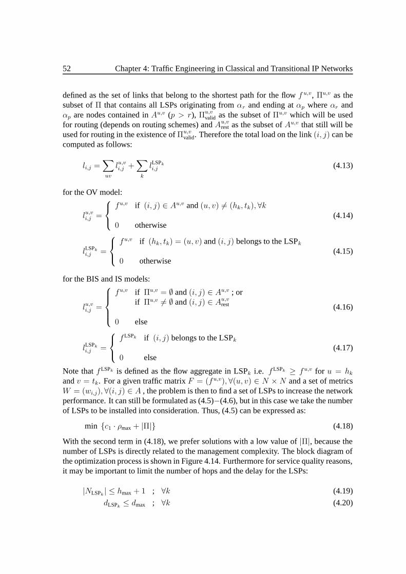
52 Chapter 4: Traffic Engineering in Classical and Transitional IP Networks
defined as the set of links that belong to the shortest path for the flowf u,v, Πu,v as thesubset ofΠ that contains all LSPs originating fromαr and ending atαp whereαr andαp are nodes contained inAu,v (p > r), Πu,v
valid as the subset ofΠu,v which will be usedfor routing (depends on routing schemes) andAu,v
rest as the subset ofAu,v that still will beused for routing in the existence ofΠu,v
valid. Therefore the total load on the link(i, j) can becomputed as follows:
li,j =∑uv
lu,vi,j +∑k
lLSPki,j (4.13)
for the OV model:
lu,vi,j =
fu,v if (i, j) ∈ Au,v and(u, v) = (hk, tk), ∀k
0 otherwise(4.14)
lLSPki,j =
fu,v if (hk, tk) = (u, v) and(i, j) belongs to the LSPk
0 otherwise(4.15)
for the BIS and IS models:
lu,vi,j =
fu,v if Πu,v = ∅ and(i, j) ∈ Au,v ; orif Πu,v = ∅ and(i, j) ∈ Au,vrest
0 else
(4.16)
lLSPki,j =
fLSPk if (i, j) belongs to the LSPk
0 else(4.17)
Note thatf LSPk is defined as the flow aggregate in LSPk i.e. f LSPk ≥ fu,v for u = hkandv = tk. For a given traffic matrixF = (fu,v), ∀(u, v) ∈ N × N and a set of metricsW = (wi,j), ∀(i, j) ∈ A , the problem is then to find a set of LSPs to increase the networkperformance. It can still be formulated as (4.5)−(4.6), but in this case we take the numberof LSPs to be installed into consideration. Thus, (4.5) can be expressed as:
min c1 · ρmax + |Π| (4.18)
With the second term in (4.18), we prefer solutions with a low value of|Π|, because thenumber of LSPs is directly related to the management complexity. The block diagram ofthe optimization process is shown in Figure 4.14. Furthermore for service quality reasons,it may be important to limit the number of hops and the delay for the LSPs:
|NLSPk| ≤ hmax + 1 ; ∀k (4.19)
dLSPk≤ dmax ; ∀k (4.20)
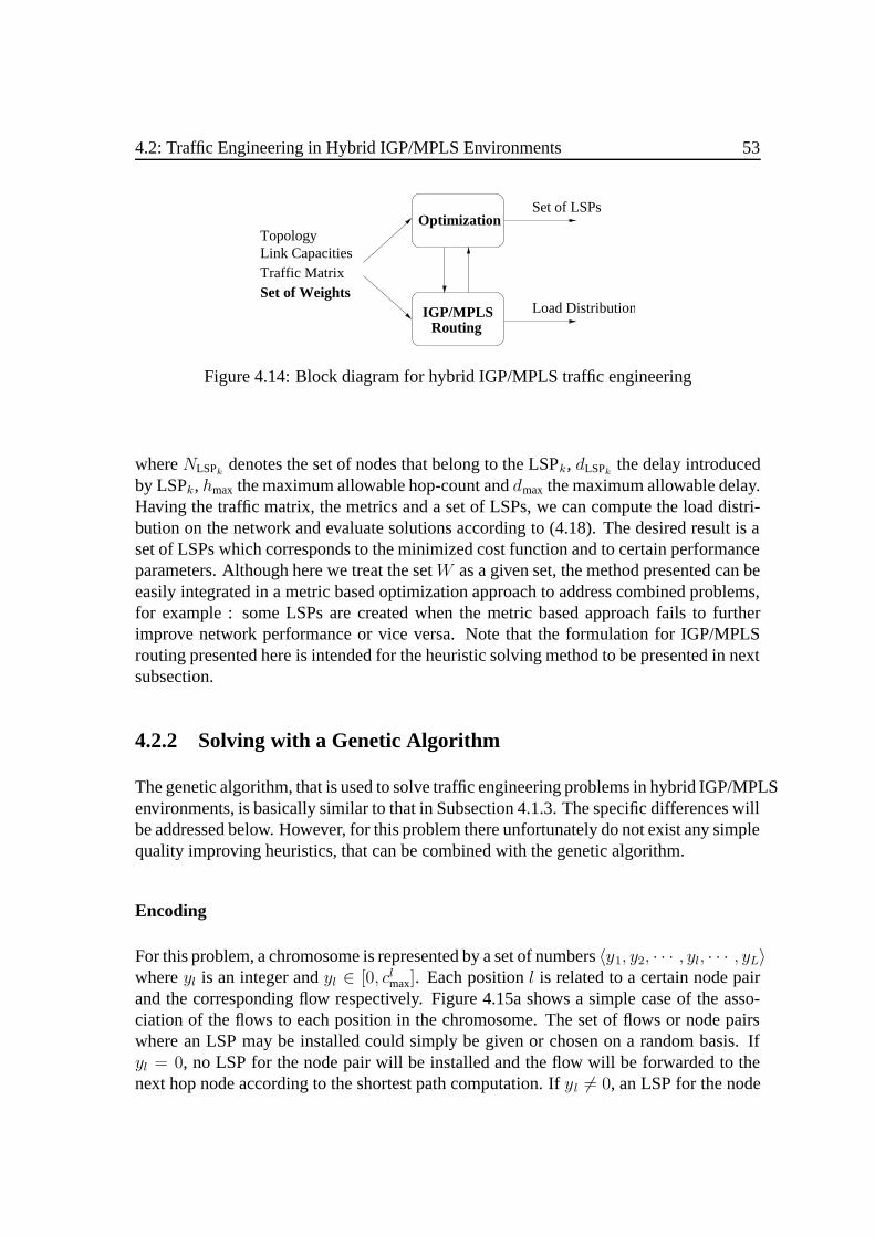
4.2: Traffic Engineering in Hybrid IGP/MPLS Environments 53
Routing
Link CapacitiesTraffic Matrix
OptimizationSet of LSPs
Load DistributionSet of Weights
IGP/MPLS
Topology
Figure 4.14: Block diagram for hybrid IGP/MPLS traffic engineering
whereNLSPkdenotes the set of nodes that belong to the LSPk, dLSPk
the delay introducedby LSPk, hmax the maximum allowable hop-count anddmax the maximum allowable delay.Having the traffic matrix, the metrics and a set of LSPs, we can compute the load distri-bution on the network and evaluate solutions according to (4.18). The desired result is aset of LSPs which corresponds to the minimized cost function and to certain performanceparameters. Although here we treat the setW as a given set, the method presented can beeasily integrated in a metric based optimization approach to address combined problems,for example : some LSPs are created when the metric based approach fails to furtherimprove network performance or vice versa. Note that the formulation for IGP/MPLSrouting presented here is intended for the heuristic solving method to be presented in nextsubsection.
4.2.2 Solving with a Genetic Algorithm
The genetic algorithm, that is used to solve traffic engineering problems in hybrid IGP/MPLSenvironments, is basically similar to that in Subsection 4.1.3. The specific differences willbe addressed below. However, for this problem there unfortunately do not exist any simplequality improving heuristics, that can be combined with the genetic algorithm.
Encoding
For this problem, a chromosome is represented by a set of numbers〈y1, y2, · · · , yl, · · · , yL〉whereyl is an integer andyl ∈ [0, clmax]. Each positionl is related to a certain node pairand the corresponding flow respectively. Figure 4.15a shows a simple case of the asso-ciation of the flows to each position in the chromosome. The set of flows or node pairswhere an LSP may be installed could simply be given or chosen on a random basis. Ifyl = 0, no LSP for the node pair will be installed and the flow will be forwarded to thenext hop node according to the shortest path computation. Ifyl = 0, an LSP for the node
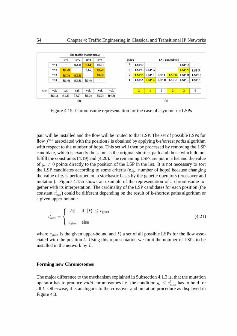
54 Chapter 4: Traffic Engineering in Classical and Transitional IP Networks
f(4,1)
f(4,2)
f(4,3)
f(3,1) f(1,2) f(4,2) f(1,3) f(2,3) f(4,3)
LSP D
LSP C
LSP B
LSP A
LSP G
LSP F
LSP E
2 1 0
LSP H
LSP I LSP K
LSP J
2
LSP O
LSP N
LSP M
LSP L
3 0
LSP R
LSP Q
LSP P
index
4
3
2
1
LSP candidates
(b)
chr. val. val. val. val. val. val.
(a)
The traffic matrix f(u,v)
u=2
−
−
−
−
v=1
v=2
v=3
v=4
f(1,2)
u=1
f(1,3)
f(1,4)
f(2,1)
f(2,3)
f(2,4)
u=3
f(3,1)
f(3,2)
f(3,4)
u=4
Figure 4.15: Chromosome representation for the case of asymmetric LSPs
pair will be installed and the flow will be routed to that LSP. The set of possible LSPs forflow fu,v associated with the positionl is obtained by applyingk-shortest pathsalgorithmwith respect to the number of hops. This set will then be processed by removing the LSPcandidate, which is exactly the same as the original shortest path and those which do notfulfill the constraints (4.19) and (4.20). The remaining LSPs are put in a list and the valueof yl = 0 points directly to the position of the LSP in the list. It is not necessary to sortthe LSP candidates according to some criteria (e.g. number of hops) because changingthe value ofyl is performed on a stochastic basis by the genetic operators (crossover andmutation). Figure 4.15b shows an example of the representation of a chromosome to-gether with its interpretation. The cardinality of the LSP candidates for each position (theconstantclmax) could be different depending on the result of k-shortest paths algorithm ora given upper bound :
clmax =
|Pl| if |Pl| ≤ cgiven
cgiven else(4.21)
wherecgiven is the given upper-bound andPl a set of all possible LSPs for the flow asso-ciated with the positionl. Using this representation we limit the number of LSPs to beinstalled in the network byL.
Forming new Chromosomes
The major difference to the mechanism explained in Subsection 4.1.3 is, that the mutationoperator has to producevalid chromosomes i.e. the conditionyl ≤ clmax has to hold forall l. Otherwise, it is analogous to the crossover and mutation procedure as displayed inFigure 4.3.

4.2: Traffic Engineering in Hybrid IGP/MPLS Environments 55
10
9
22
8
23
7
66
18
5
19
4
20
3
7
2
21
1
3
GWiN Level−2
15
26
14
27
13
9
2
24
12
25
11
4
1
16
10
5
GWiN Level−1
17
8
Figure 4.16: The G-WiN network topology
4.2.3 Results and Discussion
For the following results we used the German research and scientific network G-WiNnetwork shown in Figure 4.16. It consists of 27 nodes (10 level-1 nodes and 17 level-2nodes) and 38 bidirectional links. Each level-1 link has a transmission capacity of either2.5 Gbps or10 Gbps, while each level-2 link has either2 × 622 Mbps or2 × 2.5 Gbps[Adl02]. The traffic matrix is composed of 702 flows and each of them was generatedrandomly in the interval [4,355] Mbps. The mean demand value is 34.6 Mbps and around75% of the demands are below the value of 30 Mbps. From the topology point of view, theoptimization problem for this network could be implemented in a hierarchical way i.e. weconcentrate in optimizing the level-1 network using the aggregated flows from all level-2nodes. In this way the complexity will be drastically reduced. For instance if we considerthe total number of LSPs for a pure MPLS network, with the hierarchical approach wecould reduce the total number of LSP’s by 87%, with the assumption that each flow cannot be split. However in order to keep the generality of the method in our experimentswe used a plain approach and considered both, level-1 and level-2 networks, in the samelayer. The genetic algorithm was set to terminate if it reached a value of100 iterations orafter50 iterations with no more improvements. Delays are modeled statically and consistof three components: the propagation delaydprop, the processing and serialization delaydsp (link-rate dependent) and delay margindc. The parameter settings were : constantc1 = 1000 (Equ. 4.18), maximum hop-counthmax = 4 (Equ. 4.19),dmax = 10 ms (Equ.

56 Chapter 4: Traffic Engineering in Classical and Transitional IP Networks
IGP IGP/MPLSOV BIS IS
ρmax 0.7725 0.570338 0.523714 0.483923ρconsmax 0.7725 0.570338 0.523714 0.426447ρ 0.2345 0.237114 0.240888 0.247998
# LSP - 12 16 22
dpathmax 12.1697 12.1697 13.1659 14.8418
dpath
6.68743 6.73768 6.90382 7.23755dLSPmax - 11.1755 10.7706 10.3724
dLSP
- 8.30118 8.72935 7.56434
hpathmax 4 4 4 5
hpath
2.70085 2.71225 2.75071 2.87749ωlinkmax 58 53 45 51ωlink 24.9474 25.0526 25.4079 26.5789ωLSPmax - 1 4 12ωLSP - 1 2.9375 8.54545
Table 4.1: Some typical computation results (L = 48)
4.20),dsp = 1 ms for 622 Mbps lines anddc = 1 ms per link. In all experiments, theset of possible node pairs to be connected by an LSP is given: an LSP may be installedfor every pair of two level-1 nodes, which are not directly connected. Hence, the numberof LSPs that can be installed in the network is upper-bounded byL = 48i . The ECMPfeature was disabled and the metric value was originally set inversely proportional to thelink’s capacity. Some typical results for each hybrid scheme are displayed in Table 4.1.
Network Utilization
The most utilized link for all schemes is the level-2 link(19, 6). The traffic on level-2 linksis not reroutable, thus for the optimization they were marked asunconsideredandρmax
in (4.18) was substituted withρconsmax i.e. the maximum utilization on the level-1 network.
Using the original IGP routingρconsmax is about88% for the link(5, 6). With optimization we
can reduce the value to53.5% depending on the routing schemes and tradeoff factors (i.e.the number of LSPs to be installed). In general, a better utilization value will be obtainedby using more LSPs. For IS model by using only a few LSPs (around10%) the maximumutilization is relatively close to the best solution found in all experiments. This could bethe effect of the aggregation capability in the IS model. This aggregation capability is
iThe number of level-1 node pairs which are directly connected is 21. If all node pairs were directlyconnected, this would need 45 bidirectional links. This means 24 node pairs are not directly connected.Thus, there shall be at most 48 asymmetrical LSP candidates.

4.2: Traffic Engineering in Hybrid IGP/MPLS Environments 57
0 200 400 6000
5
10
15Source−Destination Delay (IGP)
Del
ay (
ms)
0 200 400 600−4
−2
0
2
4
6
8Source−Destination Delay (OV )
Del
ay−D
iffer
ence
(m
s)
0 200 400 600−4
−2
0
2
4
6
8Source−Destination Delay (BIS)
Del
ay−D
iffer
ence
(m
s)
Source−Destination0 200 400 600
−4
−2
0
2
4
6
8Source−Destination Delay (IS )
Del
ay−D
iffer
ence
(m
s)
Source−Destination
Figure 4.17: Source destination delays for all schemes
indicated by the parameterωLSP which denotes the number of different flows carried byan LSP. The average value ofωLSP tends to increase for the IS model.
Network Delay
Improving network utilization in all cases will increase the average delay in the network,because to avoid hot-spots the flows often must follow longer routes. By adding delayand hop constraints as in (4.19) and (4.20) we try to trade between these performance pa-rameters. Figure 4.17 shows the source-destination delay before and after optimization,for the case ofL = 48 (Table 4.1). Compared to the original IGP routing, the averagedelay at the end of the optimization increases by a value of about0.5 ms (OV),1.0 ms(BIS) and2.4 ms (IS), respectively. These differences could again be seen as a direct con-sequence of each hybrid scheme. The number of demands, which are rerouted on longerpaths for each scheme, increases from26% (OV) to 57% (IS). An almost similar case

58 Chapter 4: Traffic Engineering in Classical and Transitional IP Networks
happens for the routing hop-count: the average hop-count at the end of the optimizationincreases, at most by a value of about0.5 (IS). However, in contrast to Figure 4.17 whichindicates that some of the demands are rerouted through paths with less delay, there areno demands rerouted with less hop-count i.e. they are rerouted either through paths withequal hop-count or through those with longer hop-count.
4.3 Partial Demand Increase
Traffic in IP networks is very dynamic and tends to increase over time. By using a sim-ple linear scaling method we could easily investigate the effect of traffic increase in thenetwork. But this would not reflect reality, if we assume that traffic and its growth arestochastic quantities. In this section we consider partial demand increase and its impactson network utilization. This work has been published in [MK04a].
Contributions
To the best of our knowledge, at the time we started the research there were no publica-tions which are concerned with the issue of partial demand increase and with its impactson network performance. The scientific contributions of our work can be summarized asfollows:
• At first, our interest is to investigate the effect of partial (non-linear) traffic growthon resource occupancy and thus indirectly, on network performance. Without lossof generality, here we focus on the the classical IP networks. However, the proce-dures developed for our investigation can be applied to IP networks with differentrouting schemes.
• The second objective is to develop a policy when reoptimization should take place.Reoptimization does not make sense if partial demand increase does not result insignificant performance degradation or if traffic engineering can not give appropri-ate solutions due to e.g. network saturation, capacity limitation etc.
• Last but not least, the third objective is to develop effective reoptimization ap-proaches. If reoptimization is admitted, it is interesting to know, whether it ispossible to obtain solutions with minimal changes compared to the original con-figuration, so that in this case partial demand increase will result in only partialconfiguration changes.
This section is structured as follows. In Subsection 4.3.1 we introduce some notationsto describe and measure the effect of partial demand increase. A simple policy and two

4.3: Partial Demand Increase 59
approaches for reoptimization are explained in Subsection 4.3.2. Finally, some investiga-tions and computational results are presented in Subsection 4.3.3.
4.3.1 Notations
Let Fo = (fu,vo ), ∀(u, v) ∈ N × N be defined as the original traffic matrix, and∆Fα =(∆fu,vα ), ∀(u, v) ∈ N×N as a traffic-increase matrix whereα denotes the number of non-zero elements of∆Fα i.e. the number of source destination node pairs with increasingdemand.α can also be expressed in percentage by normalizing it with the total numberof elements in∆Fα. Our new traffic matrix, denoted byFα = (fu,vα ), ∀(u, v) ∈ N × N ,can be written as:
Fα = Fo + ∆Fα (4.22)
Note that the linear increaseF = λFo is a special case in (4.22) forα = 100% and∆Fα = (λ− 1)Fo. Increasing partially the traffic matrix could change the original trafficdistribution (see Figure 4.19) and correspondingly the original network utilization. Tomeasure these changes, two parameters can be introduced. Ifρomax denotes the originalmaximum utilization caused by distribution of the demandsFo, andραmax the maximumutilization caused byFα using the same routing pattern i.e. without changing routingconfiguration, we define the first parameter, which gives the increase of the maximumutilization introduced by demand increase∆Fα, as:
∆ραmax = ραmax− ρomax (4.23)
Furthermore, the second parameter measures the difference between maximum and aver-age utilization in the network, resulting from the new demandFα, i.e. :
∆ραdiff = ραmax− ρα (4.24)
These parameter definitions are illustrated in Figure 4.18. The left figure shows utilizationvalues before, while the right figure shows those after demand increase.
4.3.2 Policy and Reoptimization
After recalculating network parameters with the current demands, a decision should bemade whether the network has to be reoptimized. One possibility is to check the valueof the increase of the maximum utilization, that is whether∆ραmax > ε1. For illustrationconsider Figure 4.20, which shows the values of∆ραmax for the 500 samples of traffic-increase matrices∆Fα for α = 2% with ∆fu,vα randomly distributed in the inverval[5, 10]Mbps (Figure 4.20 left) and∆f u,vα ∈ [5, 50] Mbps (Figure 4.20 right) respectively. The
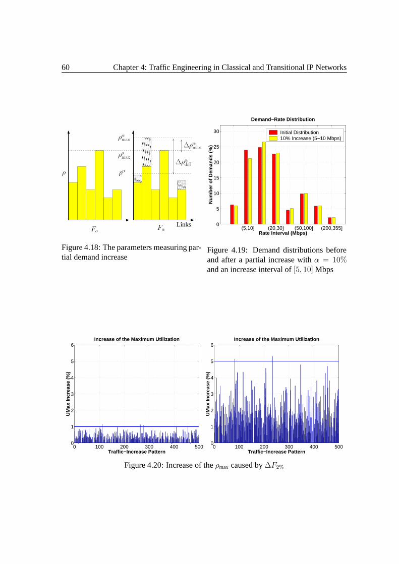
60 Chapter 4: Traffic Engineering in Classical and Transitional IP Networks
Links
∆ραdiff
∆ραmax
Fα
ρα
ραmax
Fo
ρomax
ρ
Figure 4.18: The parameters measuring par-tial demand increase
(5,10] (20,30] (50,100] (200,355]0
5
10
15
20
25
30
Demand−Rate Distribution
Num
ber
of D
eman
ds (
%)
Rate Interval (Mbps)
Initial Distribution 10% Increase (5−10 Mbps)
Figure 4.19: Demand distributions beforeand after a partial increase withα = 10%and an increase interval of[5, 10] Mbps
0 100 200 300 400 5000
1
2
3
4
5
6Increase of the Maximum Utilization
UM
ax In
crea
se (
%)
Traffic−Increase Pattern0 100 200 300 400 500
0
1
2
3
4
5
6Increase of the Maximum Utilization
UM
ax In
crea
se (
%)
Traffic−Increase Pattern
Figure 4.20: Increase of theρmax caused by∆F2%
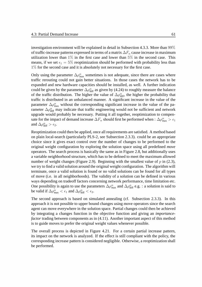
4.3: Partial Demand Increase 61
investigation environment will be explained in detail in Subsection 4.3.3. More than99%of traffic-increase patterns expressed in terms of a matrix∆Fα cause increase in maximumutilization lower than1% in the first case and lower than5% in the second case. Thismeans, if we setε1 = 5% reoptimization should be performed with probability less than1% for the second case and it is absolutely not necessary for the first case.
Only using the parameter∆ραmax sometimes is not adequate, since there are cases wheretraffic rerouting could not gain better situations. In those cases the network has to beexpanded and new hardware capacities should be installed, as well. A further indicationcould be given by the parameter∆ραdiff as given by (4.24) to roughly measure the balanceof the traffic distribution. The higher the value of∆ραdiff , the higher the probability thattraffic is distributed in an unbalanced manner. A significant increase in the value of theparameter∆ραmax without the corresponding significant increase in the value of the pa-rameter∆ραdiff may indicate that traffic engineering would not be sufficient and networkupgrade would probably be necessary. Putting it all together, reoptimization to compen-sate for the impact of demand increase∆Fα should first be performed when :∆ραmax > ε1and∆ραdiff > ε2.
Reoptimization could then be applied, once all requirements are satisfied. A method basedon plain local-search (particularly PLS-2, see Subsection 2.3.3). could be an appropriatechoice since it gives exact control over the number of changes to be performed to theoriginal weight configuration by exploring the solution space using all predefinedmoveoperators. The search process is basically the same as in Figure 2.8, but additionally usesa variable neighborhood structure, which has to be defined to meet the maximum allowednumber of weight changes (Figure 2.9). Beginning with the smallest value ofp in (2.3),we try to find a valid solution around the original weight configuration. The algorithm willterminate, once a valid solution is found or no valid solutions can be found for all typesof move (i.e. in all neighborhoods). The validity of a solution can be defined in variousways depending on tradeoff factors concerning network performance, time limitation etc.One possibility is again to use the parameters∆ραmax and∆ραdiff e.g. : a solution is said tobe valid if∆ραmax < ε1 and∆ραdiff < ε2.
The second approach is based on simulated annealing (cf. Subsection 2.3.3). In thisapproach it is not possible to upper bound changes using move operators since the searchagent can move everywhere in the solution space. Partial changes could then be achievedby integrating a changes function in the objective function and giving animportance-factor trading between components as in (4.11). Another important aspect of this methodis to guide moves to prefer the original weight values whenever possible.
The overall process is depicted in Figure 4.21. For a certain partial increase pattern,its impact on the network is analyzed. If the effect is still compliant with the policy, thecorresponding increase pattern is considered negligible. Otherwise, a reoptimization shallbe performed.

62 Chapter 4: Traffic Engineering in Classical and Transitional IP Networks
Reoptimization
Link CapacitiesTraffic MatrixPartial Increase
Analyze
Policy
success
fail
Weight Changes
Network Upgrade
policy compliant
not compliant
Topology
Figure 4.21: Block diagram for investigation of partial demand increase
4.3.3 Analysis
For the following results we used again the G-WiN network (Figure 4.16). The initialdemand distribution is shown in Figure 4.19. For each traffic-increase investigation,500increase-patterns are generated randomly with the simple rule, that only node pairs whichdo not share a common level-1 node are allowed to contribute to demand increase. This isobvious, because demand increase of node pairs sharing a common level-1 node will notaffect utilization of the links in level-1, which are our concern in this case. The values ofα used in the investigations are2%, 5%, 10%, 25% and50%. The weights were originallyset inversely proportional to links’ capacity. Setting the weights in this way caused156(around22.2%) flows to be split because of two or more ties. The average utilizationρwas23.4% and the most utilized link (ρmax = 76.6%) was the link(5, 6) which carried70 different flows. The value∆ρdiff = ρmax− ρ = 53.2% was a strong indication thatthe network was not configured appropriately and that traffic engineering actions wererequired.
For optimization, as in Subsection 4.2.3, level-2 links were marked asunconsideredandρmax in (4.11) was substituted withρcons
max i.e. the maximum utilization at the level-1 net-work. After optimization we obtain:ρcons
max = 39.4% for the link (7, 9), ρmax = 48.4%for the level-2 link(1, 12) andρ = 24.1%. Looking at these values, it is obvious thatthe optimization significantly saves network resources:∆ρcons
max = 37.2% (about930 Mbpscapacity in a2.5 Gbps link),∆ρcons
diff = 15.3% within an acceptable increase in the aver-age number of hops for routing of0.3 and an increase in average utilization from23.4%to 24.1%. With the optimized weights’ configuration, there are no split flows, since theoptimization was set to prefer unique shortest path routing.
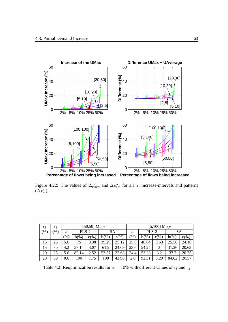
4.3: Partial Demand Increase 63
2% 5% 10% 25% 50%0
20
40
60Increase of the UMax
UM
ax In
crea
se (
%)
2% 5% 10% 25% 50%0
20
40
60Difference UMax − UAverage
Diff
eren
ce (
%)
2% 5% 10% 25% 50%0
20
40
60
UM
ax In
crea
se (
%)
Percentage of flows being increased2% 5% 10% 25% 50%
0
20
40
60
Diff
eren
ce (
%)
Percentage of flows being increase d
[50,50]
[100,100]
[5,100]
[50,50] [5,50]
[2,5]
[5,10]
[10,20]
[20,30] [20,30]
[2,5] [5,10]
[10,20]
[5,100]
[5,50]
[100,100]
Figure 4.22: The values of∆ραmax and∆ραdiff for all α, increase-intervals and patterns(∆Fα)
ε1 ε2 [50,50] Mbps [5,100] Mbps(%) (%) a PLS-2 SA a PLS-2 SA
(%) b(%) c(%) b(%) c(%) (%) b(%) c(%) b(%) c(%)15 25 5.6 75 3.38 39.29 25.12 25.8 48.84 3.63 25.58 24.1615 30 4.2 57.14 3.07 61.9 24.09 23.6 54.24 3 31.36 20.6320 25 5.6 82.14 2.52 53.57 22.63 24.4 53.28 3.2 37.7 20.2520 30 0.6 100 1.75 100 42.98 2.6 92.31 3.29 84.62 20.57
Table 4.2: Reoptimization results forα = 10% with different values ofε1 andε2
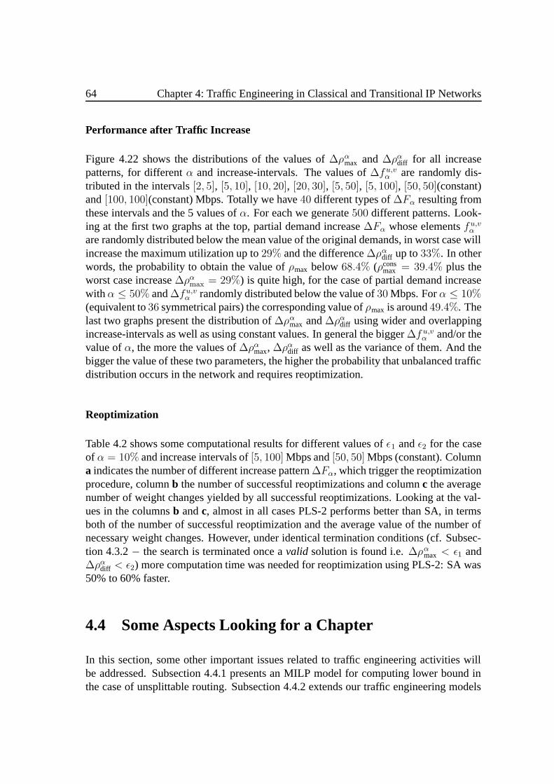
64 Chapter 4: Traffic Engineering in Classical and Transitional IP Networks
Performance after Traffic Increase
Figure 4.22 shows the distributions of the values of∆ραmax and ∆ραdiff for all increasepatterns, for differentα and increase-intervals. The values of∆f u,vα are randomly dis-tributed in the intervals[2, 5], [5, 10], [10, 20], [20, 30], [5, 50], [5, 100], [50, 50](constant)and[100, 100](constant) Mbps. Totally we have40 different types of∆Fα resulting fromthese intervals and the 5 values ofα. For each we generate500 different patterns. Look-ing at the first two graphs at the top, partial demand increase∆Fα whose elementsfu,vα
are randomly distributed below the mean value of the original demands, in worst case willincrease the maximum utilization up to29% and the difference∆ραdiff up to33%. In otherwords, the probability to obtain the value ofρmax below68.4% (ρcons
max = 39.4% plus theworst case increase∆ραmax = 29%) is quite high, for the case of partial demand increasewith α ≤ 50% and∆fu,vα randomly distributed below the value of30 Mbps. Forα ≤ 10%(equivalent to36 symmetrical pairs) the corresponding value ofρmax is around49.4%. Thelast two graphs present the distribution of∆ραmax and∆ραdiff using wider and overlappingincrease-intervals as well as using constant values. In general the bigger∆f u,vα and/or thevalue ofα, the more the values of∆ραmax, ∆ραdiff as well as the variance of them. And thebigger the value of these two parameters, the higher the probability that unbalanced trafficdistribution occurs in the network and requires reoptimization.
Reoptimization
Table 4.2 shows some computational results for different values ofε1 andε2 for the caseof α = 10% and increase intervals of[5, 100] Mbps and[50, 50] Mbps (constant). Columna indicates the number of different increase pattern∆Fα, which trigger the reoptimizationprocedure, columnb the number of successful reoptimizations and columnc the averagenumber of weight changes yielded by all successful reoptimizations. Looking at the val-ues in the columnsb andc, almost in all cases PLS-2 performs better than SA, in termsboth of the number of successful reoptimization and the average value of the number ofnecessary weight changes. However, under identical termination conditions (cf. Subsec-tion 4.3.2− the search is terminated once avalid solution is found i.e.∆ραmax < ε1 and∆ραdiff < ε2) more computation time was needed for reoptimization using PLS-2: SA was50% to 60% faster.
4.4 Some Aspects Looking for a Chapter
In this section, some other important issues related to traffic engineering activities willbe addressed. Subsection 4.4.1 presents an MILP model for computing lower bound inthe case of unsplittable routing. Subsection 4.4.2 extends our traffic engineering models

4.4: Some Aspects Looking for a Chapter 65
for dealing with network failures. Finally, in Subsection 4.4.3 we reformulate the trafficengineering problem in order to cope with network dimensioning problems.
4.4.1 Better Lower-Bounds
Since the GRP formulation presented in Section 4.1 allows bifurcated routing, as indicatedby (4.10), GRP could not give realistic lower bounds when we consider the case of singlepath routing. Thus, as far as unsplittable routing is concernedj, better lower-bounds canbe obtained by transforming GRP to Single Path Routing Problem (SPRP) as follows:
objective: (4.7)constraints: (4.8), (4.9) and
xu,vi,j =
1 if the flow fu,v is routed on link(i, j)
0 otherwise(4.25)
Looking at the objective function (4.7), although it implicitly contains a no-loop conditionfor theoptimalsolution, the following explicit no-loop constraintsk can be added:
∑∀(n,m)∈A
xu,vn,m ≤ 1 ; ∀fu,v, ∀n ∈ N (4.26)
∑∀(m,n)∈A
xu,vm,n ≤ 1 ; ∀fu,v, ∀n ∈ N (4.27)
(4.26) and (4.27) tell that the flowf u,v can arrive at and leave a nodem at most once.Furthermore, for symmetrical routing scheme (i.e. the reverse path follows the same linksin the reverse direction as the forward path), the following symmetry constraint has to befulfilled:
xu,vi,j = xv,uj,i ; ∀fu,v, ∀(i, j) ∈ A (4.28)
Link-Path Formulation
The presented formulations for GRP and SPRP are based onlink-flow variablexu,vi,j . Inthe terminology used in [PM04], such a formulation is calledNode-Linkformulation. It
jFor example, if we consider traffic engineering: (i) with unique shortest path requirements as mentionedin Section 4.1; or (ii) in hybrid IGP/MPLS environments using single path routing scheme (cf. Section 4.2).
kOur experiments with CPLEX 7.5 show that these explicit constraints can speed-up the computation(cf. [MK03], [MK04c]).
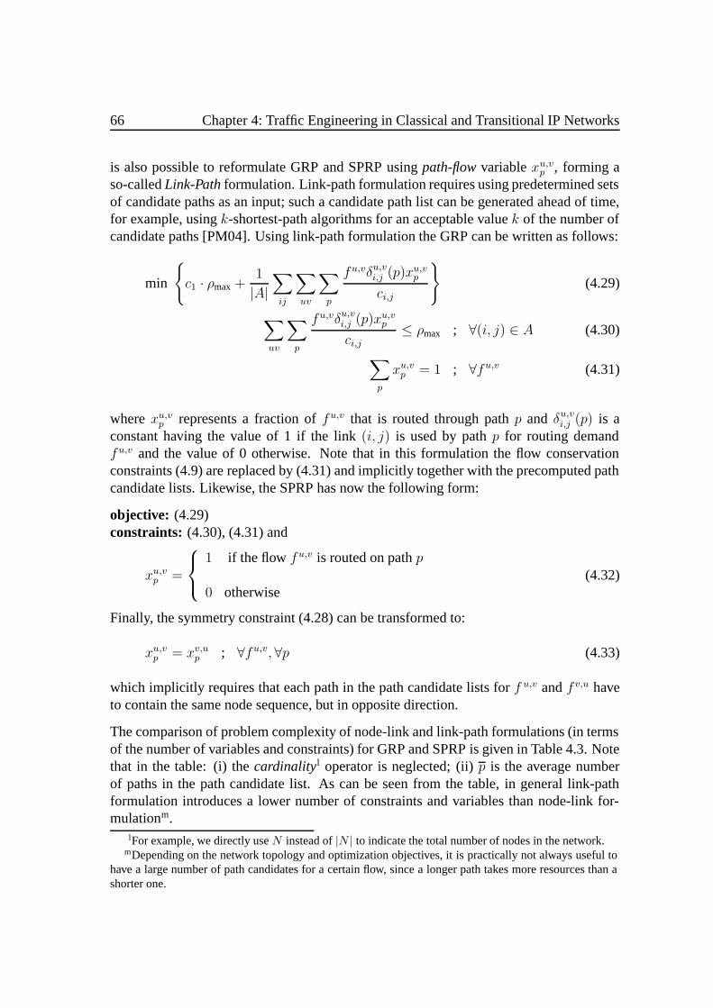
66 Chapter 4: Traffic Engineering in Classical and Transitional IP Networks
is also possible to reformulate GRP and SPRP usingpath-flowvariablexu,vp , forming aso-calledLink-Pathformulation. Link-path formulation requires using predetermined setsof candidate paths as an input; such a candidate path list can be generated ahead of time,for example, usingk-shortest-path algorithms for an acceptable valuek of the number ofcandidate paths [PM04]. Using link-path formulation the GRP can be written as follows:
min
c1 · ρmax +
1
|A|∑ij
∑uv
∑p
fu,vδu,vi,j (p)xu,vpci,j
(4.29)
∑uv
∑p
fu,vδu,vi,j (p)xu,vpci,j
≤ ρmax ; ∀(i, j) ∈ A (4.30)
∑p
xu,vp = 1 ; ∀fu,v (4.31)
wherexu,vp represents a fraction offu,v that is routed through pathp and δu,vi,j (p) is aconstant having the value of 1 if the link(i, j) is used by pathp for routing demandfu,v and the value of 0 otherwise. Note that in this formulation the flow conservationconstraints (4.9) are replaced by (4.31) and implicitly together with the precomputed pathcandidate lists. Likewise, the SPRP has now the following form:
objective: (4.29)constraints: (4.30), (4.31) and
xu,vp =
1 if the flow fu,v is routed on pathp
0 otherwise(4.32)
Finally, the symmetry constraint (4.28) can be transformed to:
xu,vp = xv,up ; ∀fu,v, ∀p (4.33)
which implicitly requires that each path in the path candidate lists forf u,v andf v,u haveto contain the same node sequence, but in opposite direction.
The comparison of problem complexity of node-link and link-path formulations (in termsof the number of variables and constraints) for GRP and SPRP is given in Table 4.3. Notethat in the table: (i) thecardinalityl operator is neglected; (ii)p is the average numberof paths in the path candidate list. As can be seen from the table, in general link-pathformulation introduces a lower number of constraints and variables than node-link for-mulationm.
lFor example, we directly useN instead of|N | to indicate the total number of nodes in the network.mDepending on the network topology and optimization objectives, it is practically not always useful to
have a large number of path candidates for a certain flow, since a longer path takes more resources than ashorter one.

4.4: Some Aspects Looking for a Chapter 67
Node-Link Link-PathGRP SPRP GRP SPRP
# real vars. N(N − 1)A+ 1 1 N(N − 1)p+ 1 1# int. vars. − N(N − 1)A − N(N − 1)p# cons. A+N(N − 1)(N +A)︸ ︷︷ ︸
α
α+ 2N2(N − 1) A+N(N − 1)︸ ︷︷ ︸β
β
Table 4.3: Comparison of the number of constraints and variables in Node-Link and Link-Path formulations for GRP and SPRP
4.4.2 Network Failures
It is unusual for the largest of the IP networks currently in operation to run for a weekwithout the failure of some network elements, be it an interface card going down, or,more rarely but more seriously, a fiber cut [GA04]. Therefore, there must be enoughcapacity in the network together with a good routing plan in order to deal with such asituation. Network failures can be categorized into: (i) link failures, which are by farthe most frequent failures in a network [SCK+03]; and (ii) node failures. For a certaintype of link failures, for examplesingle link failures, the network can be planned andconfigured so that all traffic is entirely recovered, while for the case of node failures,traffic originating and terminating at the corresponding node(s) will be blocked.
In IP networks, several activities are involved for restoration process after a failure event[Pic03]. First, the failing link has to be detected. This happens in the following way.Routers send so-called "Hello" packets. If no "Hello" packet reaches the peer after acertain time interval, then the link is considered dead. Second, new link-state packets willbe advertised. Lastly, each router recalculates the routing paths and updates its routingtable. This can take up a lot of time; in today’s IP networks this falls in the range of tensof seconds.
To address network failures, we need to reformulate our optimization problem. Lets bedefined as a possible operating condition, andS as the set of possible (normal and failure)conditions, the traffic engineering problem can now be expressed as:
min ρmax (4.34)
ρsi,j ≤ ρmax;∀(i, j) ∈ A \ Asfail, ∀s ∈ S (4.35)
whereAsfail denotes the set of links affected by failures. This formulation is genericfor both link and node failures. If a failure causes that a node is disconnected from thenetwork, the corresponding traffic matrix elements for that node are neglected, since theyare blocked. If a node fails by itself, it has to be disconnected from the network byremoving all links connecting that node with all other nodes. The rest of the optimization

68 Chapter 4: Traffic Engineering in Classical and Transitional IP Networks
Dimensioning Algorithm 1for each possible topologyq ∈ Q do
solve (4.36)−(4.37)cost(q)← 0for eache ∈ E do
establish a minimal capacityctsuch thatle
ct≤ ρc
update cost(q)end for
end forselect a possible topologyq with
minimal cost
Figure 4.23: Agreenfielddimensioning ap-proach
Dimensioning Algorithm 2for each possible topologyq ∈ Q do
solve (4.36)−(4.37)cost(q)← 0for eache ∈ E do
if (ce = 0) thenestablish a minimal capacityct
such thatlect≤ ρc
else if ( lece> ρc) then
establish a minimal capacityctsuch that le
ct+ce≤ ρc
end ifupdate cost(q) if necessaryend for
end forselect a possible topologyq with
minimal cost
Figure 4.24: A capacity expansion ap-proach
procedures remains the same as those mentioned in the preceding sections, except that asolution has to be asessed for all possible topologies as given by the failure scenarios.
4.4.3 Network Dimensioning
To address network dimensioning problems, we can also use a slightly different versionof the traffic engineering procedures explained in the previous sections. In this respect,network dimensioning is meant as determining the capacity that has to be available oneach link in the network. Two cases can be distinguished: (i)greenfielddimensioningtasks, if there are no resources available at all; and (ii) capacity expansion tasks (i.e.network upgrade), if there are already network resources available.
So far, for traffic engineering purposes, the network topology and link capacities are al-ways given. For network dimensioning purposes, this is not the case, since the topologycan be extended and the link capacity can be upgraded. For this problem setting we willintroduce heuristic approaches that need a little modification from the usual traffic engi-neering procedures. Fortunately, it is relatively simple: for a known network topology theoptimization can base directly onload instead ofutilization. That is:
min lmax (4.36)
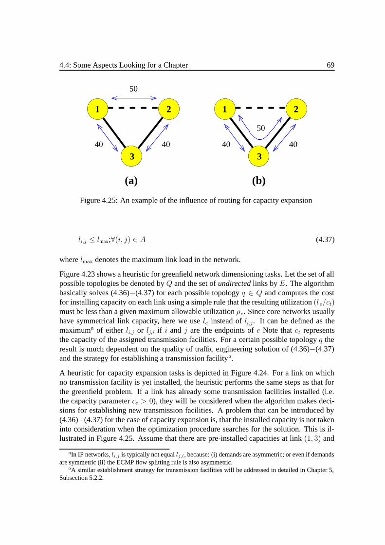
4.4: Some Aspects Looking for a Chapter 69
(a) (b)
50
3
21
40 40
50
40
1
40
2
3
Figure 4.25: An example of the influence of routing for capacity expansion
li,j ≤ lmax;∀(i, j) ∈ A (4.37)
wherelmax denotes the maximum link load in the network.
Figure 4.23 shows a heuristic for greenfield network dimensioning tasks. Let the set of allpossible topologies be denoted byQ and the set ofundirectedlinks byE. The algorithmbasically solves (4.36)−(4.37) for each possible topologyq ∈ Q and computes the costfor installing capacity on each link using a simple rule that the resulting utilization(le/ct)must be less than a given maximum allowable utilizationρc. Since core networks usuallyhave symmetrical link capacity, here we usele instead ofli,j. It can be defined as themaximumn of either li,j or lj,i if i and j are the endpoints ofe Note thatct representsthe capacity of the assigned transmission facilities. For a certain possible topologyq theresult is much dependent on the quality of traffic engineering solution of (4.36)−(4.37)and the strategy for establishing a transmission facilityo.
A heuristic for capacity expansion tasks is depicted in Figure 4.24. For a link on whichno transmission facility is yet installed, the heuristic performs the same steps as that forthe greenfield problem. If a link has already some transmission facilities installed (i.e.the capacity parameterce > 0), they will be considered when the algorithm makes deci-sions for establishing new transmission facilities. A problem that can be introduced by(4.36)−(4.37) for the case of capacity expansion is, that the installed capacity is not takeninto consideration when the optimization procedure searches for the solution. This is il-lustrated in Figure 4.25. Assume that there are pre-installed capacities at link(1, 3) and
nIn IP networks,li,j is typically not equallj,i, because: (i) demands are asymmetric; or even if demandsare symmetric (ii) the ECMP flow splitting rule is also asymmetric.
oA similar establishment strategy for transmission facilities will be addressed in detailed in Chapter 5,Subsection 5.2.2.
70 Chapter 4: Traffic Engineering in Classical and Transitional IP Networks
link (2, 3), each of 100 units. Link(1, 2) does not exist yet, but for capacity expansionpurposes it is allowed to install transmission facilities at this link. Since (4.36)−(4.37)prefer a lowest value oflmax, the routing solution in Figure 4.25a is considered better thanthat in Figure 4.25b. In fact, the first routing solution costs new transmission facilitieswhich have to be installed on link(1, 2). This is not the case for the second routing solu-tion, since the available capacity on links(1, 3) and(2, 3) is still sufficient to accomodatethe demand between node 1 and 2. To overcome such a drawback, we can explicitlyconsider the existing topology as an element inQ.

Chapter 5
Routing and Dimensioning ofMulti-Class IP/MPLS Networks
In this chapter, we focus onmulti-classIP/MPLS networks1. Two main problems will beembraced: traffic engineering and network dimensioning. In both cases, special attentionis paid to so-calledover-provisioningrequirements, since they are directly related to thequality of service. This chapter is structurized as follows. In Section 5.1 we address theoffline traffic engineering problem in such multi-class IP/MPLS networks where routingpaths are explicitly specified or determined according to the IGP metrics. In Section 5.2,we introduce some novel formulations and heuristic approaches to deal with the problemof network dimensioning under different routing schemes. Section 5.3 covers some robustdimensioning approaches, which consider LSP protection. Finally, in Section 5.4 severalremarks on LSP design will close this chapter.
5.1 Joint LSP Design and Weight Setting
Nowadays, several advanced technologies have been developed, coping with limitationsof the classical IP networks. MPLS among other things, provides a basic means to effi-ciently engineer IP traffic, while DiffServ gives the possibility to differentiate treatmentsfor IP packets with respect to their class of service. In this section, we consider the prob-lem of traffic engineering in multi-class IP/MPLS networks. As it has been previouslymentioned in Chapter 3 and Chapter 4, the main benefit of MPLS is the ability to usepaths other than shortest paths selected by the IGP to achieve a more balanced networkutilization. Such a path is called an Explicit-Route Label-Switched Path (ER-LSP). Nev-
1With the term "multi-class IP/MPLS networks" we actually point to "DS-MPLS networks" (see Chapter3).
71
72 Chapter 5: Routing and Dimensioning of Multi-Class IP/MPLS Networks
ertheless, the information provided by the IGP is still used by some label distributionprotocols e.g. to establish so-calledvanilla LSPs. A vanilla LSP is actually part of a tree,which is built by a protocol such as vanilla LDP (Label Distribution Protocol) using ex-isting IP forwarding table [SJ99]. Thus, the route of a vanilla LSP is exactly the same asthe normal IP data path. Deploying such LSPs offers several benefits: (i) no path compu-tation algorithm is necessary; (ii) the information needed for establishing LSPs is alreadyavailable in the current IGPs; this means no extension is required; (iii) a vanilla LSP canbe used as a default routing path, which can be replaced by an ER-LSP only if it doesnot satisfy the service requirements; and (iv) it is commonly argued that the number ofER-LSPs used in the network is proportionally related with the management complexity,since an ER-LSP has to be computed and stored somewhere in the network; this is not thecase for a vanilla LSP because it is set up according to the information from IGPs. Forour discussion in this chapter, we use term "LSP" and "ER-LSP" interchangeably, whilethe term "vanilla LSP" will always be stated explicitly.
In the context of multi-class IP/MPLS networks, traffic engineering could be implementedboth on per-aggregate as well as per-class basis [FL03] [FWD+02]. The termaggregateispointing to to the total demands between two nodes for all traffic classes. Using demands’aggregate, on the one hand traffic engineering may result in globally optimal performance,but on the other hand it may lead to severalper-classspecific constraints (e.g.over-provisioningconstraints) not being satisfied. Currently, Over-Provisioning (OP) is a usualand practical way for ISPs to provide a certain level of QoS in their networks and it seemsthat it will still be an important aspect in providing QoS for IP networks in the future. OPbasically means avoiding overload by ensuring that capacity of all links is greater thandemand both in normal or in failure situations [Rob01]. For some cases, as addressedin [FE02], OP based on traffic aggregate can be more expensive than that based on eachtraffic class, for instance if the portion of important traffic in a backbone is much less thanthat of normal best-effort traffic.
Contributions
As our main contributions, in this section we present an offline traffic engineering ap-proach for the problem of per-class unsplittable routing in multi-class IP/MPLS networksto specifically address per-class over-provisioning traffic constraints. As managementcomplexity may be increased by installing a large number of ER-LSPs, we adapt a hy-brid routing strategy, where packets can be routed using both vanilla LSPs based on IGPlink metrics and ER-LSPs, which are established only to achieve better performance or toobtain a feasible routing solution if one or more constraints are violated. This work haspreviously been reported in [MK05c].
The remainder of this section is organized as follows. The following subsection introducessome notations and mathematically describes the problem of unsplittable per-class traffic

5.1: Joint LSP Design and Weight Setting 73
(c)(a) (b)
3
5 6
VanillaLSP
1 2
5
5
3
2
1 2
2
LSPER−
21
65
43
1
2
4
6
5
3
4
Figure 5.1: Routing in an IP/MPLS network using both vanilla and ER-LSPs
engineering problem using both vanilla and ER-LSPs. In Section 5.1.2 we discuss theheuristic which will be used for solving the problem. Lastly, in Section 5.1.3 we presentsome results for the case of two and three traffic classes.
5.1.1 Problem Description
MPLS introduces routing flexibility, which is very important from an operator’s point ofview, e.g. to implement policy-based or QoS-based routing for certain classes of trafficin the network. Together with DiffServ, it can be used to implement a so-called per-classunsplittable MPLS routing scheme, where: (i) a demand for a certain source, destinationand class of traffic can not be split and has to be carried by one LSP (either vanilla or ER-LSP); and (ii) demands with different traffic classes for the same source and destinationare routed by LSPs, which do not necessarily have to follow the same route. This isillustrated in Figure 5.1. Figures 5.1a and 5.1b show the metric values and the shortestpath tree similar to Figure 4.1a. Figure 5.1c depicts two (vanilla and ER-) LSPs used forrouting from node1 to node6. The vanilla LSP follows the same route as the IP data path(1−3−4−6), while the ER-LSP could be set differently e.g. through the node sequence(1 − 2 − 4 − 6). In the context of per-class unsplittable MPLS routing, each LSP forthe same source and destination node will carry a different class of traffic e.g. in Figure5.1c vanilla LSP could be used forbest-efforttraffic, while ER-LSP forpremiumtraffic orvice versa. Since vanilla LSPs are built using IP forwarding tables, which are determinedby shortest path computation with respect to IGP link metrics, routing optimization canbe performed in the same way as for pure IGP networks i.e. by directly optimizing linkmetrics as addressed in Chapter 4. By ER-LSPs it is more flexible: a path can completelybe specified by the source. In spite of this, it is commonly argued that networks relying
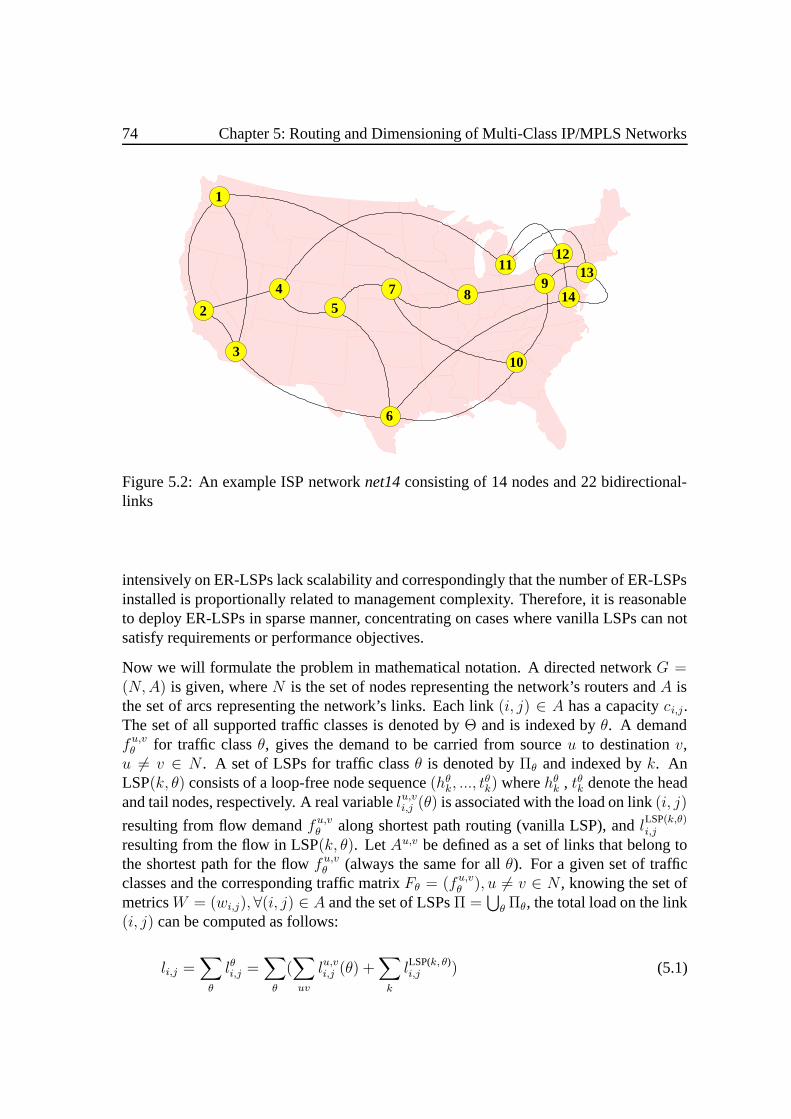
74 Chapter 5: Routing and Dimensioning of Multi-Class IP/MPLS Networks
142
3
45
6
7 8
10
119
1213
1
Figure 5.2: An example ISP networknet14consisting of 14 nodes and 22 bidirectional-links
intensively on ER-LSPs lack scalability and correspondingly that the number of ER-LSPsinstalled is proportionally related to management complexity. Therefore, it is reasonableto deploy ER-LSPs in sparse manner, concentrating on cases where vanilla LSPs can notsatisfy requirements or performance objectives.
Now we will formulate the problem in mathematical notation. A directed networkG =(N,A) is given, whereN is the set of nodes representing the network’s routers andA isthe set of arcs representing the network’s links. Each link(i, j) ∈ A has a capacityci,j.The set of all supported traffic classes is denoted byΘ and is indexed byθ. A demandfu,vθ for traffic classθ, gives the demand to be carried from sourceu to destinationv,u = v ∈ N . A set of LSPs for traffic classθ is denoted byΠθ and indexed byk. AnLSP(k, θ) consists of a loop-free node sequence(hθk, ..., t
θk) wherehθk , tθk denote the head
and tail nodes, respectively. A real variablelu,vi,j (θ) is associated with the load on link(i, j)
resulting from flow demandf u,vθ along shortest path routing (vanilla LSP), andlLSP(k,θ)i,j
resulting from the flow in LSP(k, θ). LetAu,v be defined as a set of links that belong tothe shortest path for the flowf u,vθ (always the same for allθ). For a given set of trafficclasses and the corresponding traffic matrixFθ = (fu,vθ ), u = v ∈ N , knowing the set ofmetricsW = (wi,j), ∀(i, j) ∈ A and the set of LSPsΠ =
⋃θ Πθ, the total load on the link
(i, j) can be computed as follows:
li,j =∑θ
lθi,j =∑θ
(∑uv
lu,vi,j (θ) +∑k
lLSP(k, θ)i,j ) (5.1)

5.1: Joint LSP Design and Weight Setting 75
OptimizationTopology
Per−ClassTraffic Matrices
ER−LSPs(vanilla LSPs)Set of Weights
OP Constraints
Metric−BasedTraffic Engineering
Link Capacities
Figure 5.3: Block diagram for joint LSP design and weight setting
where
lu,vi,j (θ) =
fu,vθ if (i, j) ∈ Au,v and(u, v) = (hθk, tθk), ∀k
0 otherwise(5.2)
lLSP(k, θ)i,j =
fu,vθ if (u, v) = (hθk, tθk) and(i, j) belongs to the LSP(k, θ)
0 otherwise(5.3)
The capacity on a link has to be available for all demands that are routed through that linki.e. the following constraints have to be satisfied.
ρmax = max(i,j)∈A
li,jci,j ≤ 1 (5.4)
λθmin = min(i,j)∈A
c∗θi,j
lθi,j ≥ cOP
θ , ∀θ ∈ Θ (5.5)
(5.4) is the utilization upper-bound constraint for aggregate traffic while (5.5) is the min-imum OP constraint for traffic classθ. Note thatcOP
θ denotes the given minimum OPfactor for traffic classθ andc∗θi,j = ci,j −
∑θ−1s=1 l
si,j the residual link capacityavailable
for traffic classθ, assuming that the setΘ is ordered from high to low priority traffic (i.e.θ = 1 more important thanθ = 2 · · · ). Thus, the problem of per-class unsplittable MPLSrouting using vanilla and ER-LSPs is to find the set of metric valuesW and the set of LSPΠ, such that network resources are used efficiently while satisfying the constraints. Dueto the management complexity reasons by applying ER-LSPs, this problem can thereforebe seen as a multi-objective optimization problem: (i) to optimize network resources e.g.by minimizingρmax; and (ii) to minimize management complexity i.e. in terms of|Π|.

76 Chapter 5: Routing and Dimensioning of Multi-Class IP/MPLS Networks
A Heuristic for Installing LSPsΠ← ∅; fail ← false;optimize network(F )→ RT ;if (λθmin ≥ cOP
θ ;∀θ) then break;for eachi ∈ Θ do
optimize network(Fi)→ RTi;compare(RT,RTi);updateΠ;if (λθmin ≥ cOP
θ ;∀θ) then break;if (λimin < cOP
i ) then fail ← true; break;end for
Figure 5.4: A heuristic for installing LSPs
50 100 150 200 250 300 350 400 450 5000
2000
4000
6000
8000
10000
12000
14000
16000
18000SA Convergence (Aggregate Demands)
Obj
ectiv
e V
alue
s
Iteration Number
Objective values of current−agent
Objective values of best−agent
Temperature
Figure 5.5: The convergence characteristicof the hybrid SA applied to aggregate de-mands
The block diagram for the optimization process is illustrated in Figure 5.3. As can be seenfrom the figure and as it will be addressed in the next subsection, we solve the problemindirectlyusing a metric-based traffic engineering approach, where (5.4) and (5.5) are im-plemented assoftconstraints i.e. during the search process they can be violated. At theend of the optimization, it will then be checked whether the solution is valid and satisfiesboth constraints.
5.1.2 A Solving Strategy
Figure 5.4 shows the heuristic used for solving the problem. It makes use of a trafficengineering procedure based on simulated annealing (cf. Subsections 2.3.4 and 4.3.2),that returns a set of metric values (a weight-system)W and the corresponding routingpatterns for the given demands, each time it is called by the heuristic. The traffic en-gineering procedure will search for a weight-system that results inuniqueshortest pathrouting and optimizes the objective function (4.5). In the first step, the network willbe optimized using the demand aggregateF =
∑θ Fθ . The resulting weight-system
W o = (woi,j), ∀(i, j) ∈ A is used as IGP metrics for establishing vanilla LSPs. After-wards, it will be checked whether the constraints (5.4) and (5.5) are already satisfied.If it is the case, no further steps are necessary. Otherwise several ER-LSPs have to beinstalled and the heuristic calls the metric-based traffic engineering procedure in each it-eration using the traffic matrix for the corresponding traffic class. The resulting routingpattern (RTi) is compared with that resulting fromW o (RT ). Routing entries inRTi,
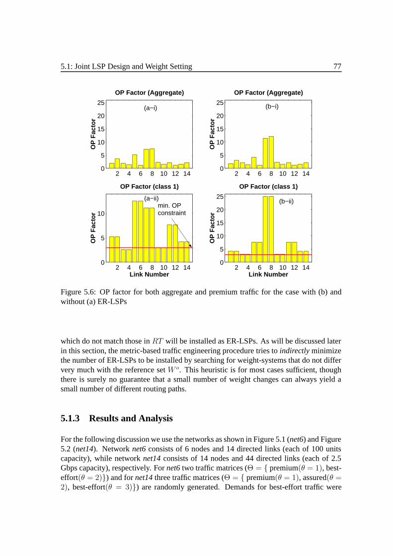
5.1: Joint LSP Design and Weight Setting 77
2 4 6 8 10 12 140
5
10
15
20
25
OP Factor (Aggregate)O
P F
acto
r
2 4 6 8 10 12 140
5
10
15
20
25
OP Factor (Aggregate)
OP
Fac
tor
2 4 6 8 10 12 140
5
10
OP Factor (class 1)
OP
Fac
tor
Link Number2 4 6 8 10 12 14
0
5
10
15
20
25
OP Factor (class 1)
OP
Fac
tor
Link Number
(a−i)
(a−ii)
(b−i)
(b−ii) min. OP constraint
Figure 5.6: OP factor for both aggregate and premium traffic for the case with (b) andwithout (a) ER-LSPs
which do not match those inRT will be installed as ER-LSPs. As will be discussed laterin this section, the metric-based traffic engineering procedure tries toindirectlyminimizethe number of ER-LSPs to be installed by searching for weight-systems that do not differvery much with the reference setW o. This heuristic is for most cases sufficient, thoughthere is surely no guarantee that a small number of weight changes can always yield asmall number of different routing paths.
5.1.3 Results and Analysis
For the following discussion we use the networks as shown in Figure 5.1 (net6) and Figure5.2 (net14). Networknet6consists of 6 nodes and 14 directed links (each of 100 unitscapacity), while networknet14consists of 14 nodes and 44 directed links (each of 2.5Gbps capacity), respectively. Fornet6two traffic matrices (Θ = premium(θ = 1), best-effort(θ = 2)) and fornet14three traffic matrices (Θ = premium(θ = 1), assured(θ =2), best-effort(θ = 3)) are randomly generated. Demands for best-effort traffic were
78 Chapter 5: Routing and Dimensioning of Multi-Class IP/MPLS Networks
produced using the hot-spot model as introduced in [FT00]: the demand between nodesuandv is proportional toOuDvCu,ve−d(u,v)/2∆, whereOu,Dv andCu,v are random numbersin the interval[0, 1], d(u, v) is the distance between each pair of nodes(u, v) and∆ is thelargest Euclidean distance between any pair of nodes. The numbersOu andDv modelthat different nodes can be more or less active senders and receivers, thus modeling hotspots in the network. The factore−d(u,v)/2∆ implies that we have relatively more demandbetween close pair of nodes. Demands for premium and assured traffic were just takenrandomly from several predefined demand values in the intervals:[4, 10] for net6(θ = 1),[10, 150] for net14(θ = 1) and [10, 70] for net14(θ = 2). The resulting mean demandvalues for each traffic class are:(5.067; 7.58) units for net6; and (49.56; 36.98; 68.58)Mbps fornet14, respectively.
Convergence
Figure 5.5 shows the convergence characteristic of the hybrid SA applied tonet14usingtraffic aggregateF . The parameters were set as follows. The search terminates if themaximum number iterations of 500 or the maximum number iterations without improve-ments of 300 is exceeded. The equilibrium for temperature T is reached if the numberof iterations without improvements at that temperature exceeds the value of 30.σPLS (cf.Subsection 2.3.6) is set to have the value of 1 if the current number of iterations withoutimprovements is less than the value of 25. The figure shows that from the start and at asmall number of iterations, the algorithm performs plain local-search since improvementsalways exist at least every 25 iterations. Once the value is exceeded, the algorithm per-forms the normal SA till the next event for PLS is triggered i.e. a new value for best agentis found. Looking at the SA parts in the figure, the impact of temperature values on themoves is very obvious. High temperatures imply high acceptance probabilities for mov-ing towards less performing solutions, while at low temperatures only moderate movesare allowed.
OP Factor and Link Utilization
The common rule-of-thumb for capacity provisioning is to have a minimum OP factorlarger than2.0 or correspondingly a maximum utilization below50.0%. For dealing withnetwork failure situations or unexpected traffic demands, several network providers mightwant to have larger OP factors. For the following experiments, we always set the valueof cOP
θ for θ other than best-effort traffic larger than2.0. Figure 5.6 shows OP factor fornet6after optimization by using: (i) the traffic aggregateF , where all demands regard-less of their classes are routed using vanilla LSPs; and (ii) the traffic matrixFθ=1, whereseveral demands are routed using ER-LSPs. The minimum OP factor for premium traf-fic was set to3.0. This can not be achieved without ER-LSPs, since optimization using

5.1: Joint LSP Design and Weight Setting 79
0 10 20 30 400
20
40
60
80
100U
tiliz
atio
n (%
)Link Utilization
class 1class 2class 3
0 10 20 30 400
20
40
60
80
100
Util
izat
ion
(%)
Link Utilization
class 1class 2class 3
0 10 20 30 400
5
10
15
20
OP Factor (class 1)
OP
Fac
tor
0 10 20 30 400
5
10
15
20
OP Factor (class 1)
OP
Fac
tor
0 10 20 30 400
10
20
30
OP Factor (class 2)
OP
Fac
tor
Link Number0 10 20 30 40
0
10
20
30
OP Factor (class 2)
OP
Fac
tor
Link Number
(a−i)
(a−ii)
(a−iii)
(b−i)
(b−ii)
(b−iii)
min. OP constraint
Figure 5.7: Link utilization and OP factor with (b) and without (a) ER-LSPs for the caseof 3 traffic classes, applied tonet14.
traffic aggregateF results inλθ=1min = 2.63. Thus, further steps as shown in Figure 5.4 are
necessary. Applying optimization usingFθ=1 results inλθ=1min = 3.03 which now satifies
the requirement. This is achieved: (i) by installing a symmetrical LSP for the premiumtraffic; and (ii) at the cost of a small decrease in the minimum OP factor for aggregatetraffic from 1.26 (without the LSP) to1.19 (with the LSP). The corresponding graphsfor net14are shown in Figure 5.7. After the first step we have the maximum utilizationfor aggregate traffic of96.44% and the minimum OP factor values of(3.00; 3.38; 1.07)for the premium, assured and best-effort traffic, respectively (Figure 5.7a). By settingthe minimum OP constraints to(4.0; 4.0; 1.0) we need again to reroute some of the traf-fic using ER-LSPs. After optimization usingFθ=1 andFθ=2, ρmax decreases to93.68%and the minimum OP factor values of(4.05; 4.01; 1.07) can be achieved by installing 13symmetrical LSPs for premium and 4 symmetrical LSPs for assured traffic. Figure 5.7b-

80 Chapter 5: Routing and Dimensioning of Multi-Class IP/MPLS Networks
ii and 5.7b-iii show the resulting OP factor for each link forθ ∈ 1, 2. Although theminimum OP constraints are already satisfied, the optimization can be applied forFθ=3
to investigate whether a better solution is available. In our case, after optimizationλθ=3min
is improved from1.07 to 1.14 while ρmax decreases to92.25%. This happens at the costof additional 9 symmetrical LSPs that have to be installed forθ = 3. The resulting linkutilizations are shown in Figure 5.7b-i.
5.2 Network Dimensioning
Internet Service Providers are confronted with increasing business competition. Oneof the important aspects is how they can provide better and new inovative services andkeep investment and operational costs as low as possible while maximizing revenues andguaranteeing grades of service. From ISPs’ point of view this means that they have toprovision and adapt their networks efficiently subject to services offered to their cus-tomers. In this section we address the problem of IP/MPLS network dimensioning tosupport differentiated services under per-class over-provisioning constraints with severaldifferent routing schemes. Furthermore, as in the preceding section, we also considerOver-Provisioningconstraints as a means to provide a certain level of quality of service.Besides, it is also useful for dealing with large variation in traffic demand or with delaysrequired for link capacity upgrade due to current technology limitations. In the contextof multi-class IP networks, OP requirements can be deployed both based on per-class orper-aggregate traffic. We also focus on per-class OP constraints, since per-class OP is themore general situation and for most cases it is economically cheaper than OP applied tothe total traffic [FE02].
Contributions
The problem of IP network dimensioning using DiffServ architecture is relatively newand therefore, to the best of our knowledge, there are only a few publications in this areae.g. [WR03]. In this regard, our main contributions are in the following aspects:
• We use a simple per-class OP mechanism as a means for providing QoS.
• We present several novel (M)ILP formulations for the problem, with several differ-ent routing schemes.
• We propose a simple and flexible heuristic approach that can be extended by orcombined with metaheuristic-based optimization frameworks.
This work has previously been published in [MSK05].

5.2: Network Dimensioning 81
2,(1,6) 2,(1,6)h
h1,(1,6)
2,(1,6)
4
5 6
1 1 2
1
11
0
1
1
1 2
3 4
5 6
(a) (b) (c)
1
10
0
0
0
1 2
3 4
5 6
2
20
0
0
0
1 2
3
h
h1,(1,6)h1,(1,6)
h
Figure 5.8: Some illustrations showing the number of transport modules to be installedfor different routing strategies and over-provisioning constraints, see text.
The problem and corresponding solving approach considered in section can be appliedto both using the classical technology, where the necessary connections are leased fromand established by carriers, or using the future technology, where the circuits can beestablished and released on demand by the ISPs. The first case is represented e.g. bythe IP over SDH (Synchronous Digital Hierarchy) architecture, where the ISPs have todecide which and how many STM (Synchronous Tranport Module) lines on which linksshould be installed to accomodate all demand and QoS requirements. The latter casecan be represented e.g. by the IP over OTN (Optical Transport Networks) architecture,assuming that carriers offer a non-linear cost structure giving benefits for establishing alarger capacity between two arbitrary nodes in their networks.
The remainder of this section is structured as follows. The following subsection intro-duces some notations and mathematically describes the problems of dimensioning ofmulti-class over-provisioned IP networks. In Section 5.2.2 we discuss the heuristic whichwill be used for solving the problems. Finally, in Section 5.2.3 we present some resultsfor the case of two sample networks.
5.2.1 Mathematical Formulation
As explained in Chapter 3, in multi-class (DiffServ) IP networks, it is possible to per-form class-based routing i.e. different LSPs for the same egress-ingress pair are used fordifferent classes of traffic, so that the physical network is divided into multiple virtual net-works: one for each traffic class [XHBN00]. Here, two routing schemes are considered:(i) per-class routing scheme, where LSPs of different traffic classes for the same node pair
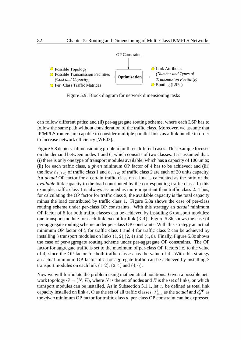
82 Chapter 5: Routing and Dimensioning of Multi-Class IP/MPLS Networks
Possible Topology Link Attributes
Routing (LSPs)
(Number and Types ofTransmission Facitility)
Optimization
OP Constraints
Possible Transmission Facilities(Cost and Capacity)Per−Class Traffic Matrices
Figure 5.9: Block diagram for network dimensioning tasks
can follow different paths; and (ii) per-aggregate routing scheme, where each LSP has tofollow the same path without consideration of the traffic class. Moreover, we assume thatIP/MPLS routers are capable to consider multiple parallel links as a link bundle in orderto increase network efficiency [WE03].
Figure 5.8 depicts a dimensioning problem for three different cases. This example focuseson the demand between nodes1 and6, which consists of two classes. It is assumed that:(i) there is only one type of transport modules available, which has a capacity of 100 units;(ii) for each traffic class, agivenminimum OP factor of4 has to be achieved; and (iii)the flowh1,(1,6) of traffic class1 andh2,(1,6) of traffic class2 are each of 20 units capacity.An actual OP factor for a certain traffic class on a link is calculated as the ratio of theavailablelink capacity to the load contributed by the corresponding traffic class. In thisexample, traffic class1 is always assumed as more important than traffic class2. Thus,for calculating the OP factor for traffic class2, the available capacity is the total capacityminus the load contributed by traffic class1. Figure 5.8a shows the case of per-classrouting scheme under per-class OP constraints. With this strategy anactual minimumOP factor of5 for both traffic classes can be achieved by installing6 transport modules:one transport module for each link except for link(3, 4). Figure 5.8b shows the case ofper-aggregate routing scheme under per-class OP constraints. With this strategy an actualminimum OP factor of5 for traffic class1 and4 for traffic class2 can be achieved byinstalling3 transport modules on links(1, 2),(2, 4) and(4, 6). Finally, Figure 5.8c showsthe case of per-aggregate routing scheme under per-aggregate OP constraints. The OPfactor for aggregate traffic is set to the maximum of per-class OP factors i.e. to the valueof 4, since the OP factor for both traffic classes has the value of4. With this strategyan actual minimum OP factor of5 for aggregate traffic can be achieved by installing2transport modules on each link(1, 2), (2, 4) and(4, 6).
Now we will formulate the problem using mathematical notations. Given a possible net-work topologyG = (N,E), whereN is the set of nodes andE is the set of links, on whichtransport modules can be installed. As in Subsection 5.1.1, letce be defined as total linkcapacity installed on linke, Θ as the set of all traffic classes,λθmin as theactualandcOP
θ asthegivenminimum OP factor for traffic classθ, per-class OP constraint can be expressed

5.2: Network Dimensioning 83
by inequality (5.5). Depending on routing schemes and types of OP requirements, in thefollowing, several problem variants can be defined. Nevertheless, all problems follow thesame principle as depicted in Figure 5.9. Using link-path notations, the first problem i.e.the problem of network dimensioning using per-class routing scheme under per-class OPconstraints (denoted by5.2-P1) can be defined as follows:
5.2-P1 Network dimensioning using per-class routing scheme under per-class OP constraints
objective:
minimize ψ =∑e
∑t
ξt · yet (5.6)
constraints:
∑d
∑p
δedp
(cOPθ · xθdp +
θ−1∑i=1
xidp
)≤∑t
yet · kt, ∀θ, ∀e (5.7)
∑p
uθdp = 1, ∀θ, ∀d (5.8)
xθdp = hθd · uθdp, ∀θ, ∀d, ∀p (5.9)
Table 5.1 lists some notations which are used in the formulation. Inequality (5.7) definesthe capacity constraints under consideration of per-class OP factors. The equations (5.8)and (5.9) assure that demand volumehθd is entirely routed. Using per-aggregate routingscheme the problem of network dimensioning under per-class OP constraints (denoted by5.2-P2) can be expressed by:
5.2-P2 Network dimensioning usingper-aggregate routing scheme underper-class OP constraints
objective:
minimize ψ =∑e
∑t
ξt · yet
constraints: (5.7) and

84 Chapter 5: Routing and Dimensioning of Multi-Class IP/MPLS Networks
sets:indicesΘ : θ traffic classes
T : t, r types of transport modules (transmission facility)D : d demands (node pairs)Pd : p candidate paths for flows realizing demanddE : e links
constantsδedp = 1, if link e belongs to pathp realizing demandd;
= 0, otherwisehθd volume of demandd for classθcOPθ given minimum OP factor for classθ
cOPaggr given minimum OP factor for aggregate traffic
ξt(ξr) cost for a transport module of typet(r)kt(kr) capacity of a transport module of typet(r)
variablesxθdp flow fraction of demandd of classθ allocated to pathpuθdp flow fraction corresponding toxθdp (normalized); binary variable for the
case single path (SP) routing schemexdp flow fraction of demandd (aggregate) allocated to pathpudp flow fraction (normalized) corresponding toxdp for problem5.2-P3; flow
fraction (normalized) corresponding toxθdp, ∀θ for problem5.2-P2; binaryvariable for the case single path (SP) routing scheme
yet(yer) number of transport modules of typet(r) on link e
Table 5.1: Some notations used in the formulation
∑p
udp = 1, ∀d (5.10)
xθdp = hθd · udp, ∀θ, ∀d, ∀p (5.11)
Looking at the formulations above, it is clear that the problem5.2-P2is almost identicalto 5.2-P1except that (5.10)(5.11) uses aggregate routing variableudp instead of per-classvariableuθdp as in (5.8) and (5.9). Finally, the problem of network dimensioning usingper-aggregate routing scheme under per-aggregate OP constraints (denoted by5.2-P3)can be formulated as the following simple network design problem:

5.2: Network Dimensioning 85
5.2-P3 Network dimensioning usingper-aggregate routing scheme underper-aggregate OP constraints
objective:
minimize ψ =∑e
∑t
ξt · yet
constraints: (5.10) and
cOPaggr
∑d
∑p
δedp · xdp ≤∑t
yet · kt, ∀e (5.12)
xdp = udp∑θ
hθd, ∀d, ∀p (5.13)
Note that: (i) the constantcOPaggr in (5.12) is set tomaxθcOP
θ in order to give a clear com-parison of the impact of per-class and per-aggregate OP constraints; and (ii) a single path,denoted by SP, per-class (per-aggregate) routing scheme can be obtained by constraininguθdp (udp) as a binary variable, while for a multi-path, denoted by MP, case the variablecan be an arbitrary real number between 0 and 1.
5.2.2 A Heuristic Approach
As alternative to the (M)ILP approach presented in Subsection 5.2.1 and since networkdesign problems with modular costs belong to NP complete problems [PM04], in this sub-section we present a flexible heuristic approach which can be used for both random as wellas for metaheuristic-based optimization frameworks. The proposed algorithm is shownin Figure 5.10 and belongs togreedyheuristics in the sense that decisions for demand-path allocation are based on the incremental cost triggered by each possible allocation.The benefits of such heuristics for solving various design and optimization problems inthe area of communication networks have been previously investigated e.g. in [BK99][Bec01].
The algorithm starts by setting the costψ to zero. This can be thought of either as agreen-fieldapproach or as a network expansion approach where no cost is charged for using theexisting free resources. Then for each demandd in a certain sequence of the elements inD and for each classθ of the corresponding demandd, the algorithm calculates the incre-mental costs, which are possibly caused by the allocations of demandhθd to all consideredpath candidates. The demandhθd is then allocated to the cheapest pathp, the necessarytransport modules are installed, the overall costψ is updated and the algorithm processesthe nextθ or d. Using this approach we can transform the dimensioning problems to a

86 Chapter 5: Routing and Dimensioning of Multi-Class IP/MPLS Networks
Greedy Algorithm ALG −1ψ← 0;loop (L1) for eachd do
loop (L2) for eachθ doloop (L3) for eachp do
calculate∆ψ(p);end (L3)choose the cheapest pathp;update the nework if necessary;establish demandd on pathp;ψ ← ψ + ∆ψ(p);
end (L2)end (L1)
Figure 5.10: A greedy heuristic for network dimensioning
sequential orderingproblem (cf. Subsection 2.3.2) of the demands inD. The incrementalcost for establishing a demandhθd on a certain pathp is the sum of the incremental costsof all links in that path, that is∆ψ(p) =
∑e∈p ∆ψ(e). Before computing the incremental
cost∆ψ(e), we first define a condition that is required in order to give benefits for usingtransport modules with higher capacities. Assuming the setT is ordered from low to highcapacity i.e.kt=1 < kt=2 < · · · , a transport modulet + 1 will be used if the costξt+1
is lower than the multiplication of the capacity gainkt+1/kt and the costξt, that is if thefollowing condition is fulfilled.
kt+1
kt>ξt+1
ξt, ∀t ∈ 1, · · · , |T | − 1 (5.14)
The incremental cost∆ψ(e) is computed as follows. Letψo(e) =∑
t ξt · yet be definedas the total cost of transport modules currently installed on linke. Now, if by adding theloadhθd on e, all capacity and OP requirements are still satisfied, then∆ψ(e) = 0 andfurther steps are not necessary. Otherwise a minimal number of transport modules of typet = 1 has to be additionally installed one, such that all OP constraints are fulfilled. Thenit has to be checked if it is necessary to replace some transport modules of lower capacitywith one or more transport modules of higher capacity in order to reduce costs. Thus, foreacht ∈ 1, · · · , |T | − 1, the following transport modules’ replacement strategy has torepeatedly be applied for a certaint till the condition
∑tr=1 ξr · yer < ξt+1 is satisfied:
if (t∑
r=1
kr · yer ≤ kt+1)→ yer = 0, ∀r ∈ 1, · · · , t and ye(t+1) = ye(t+1) + 1 (5.15)
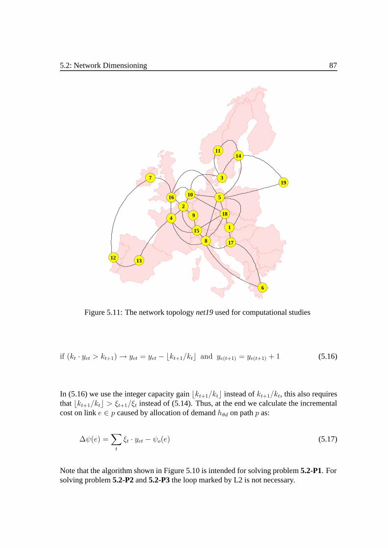
5.2: Network Dimensioning 87
6
12 13
16
4
2
10
9
15
8
1114
3
5
19
18
1
17
7
Figure 5.11: The network topologynet19used for computational studies
if (kt · yet > kt+1)→ yet = yet − kt+1/kt and ye(t+1) = ye(t+1) + 1 (5.16)
In (5.16) we use the integer capacity gainkt+1/kt instead ofkt+1/kt, this also requiresthatkt+1/kt > ξt+1/ξt instead of (5.14). Thus, at the end we calculate the incrementalcost on linke ∈ p caused by allocation of demandhθd on pathp as:
∆ψ(e) =∑t
ξt · yet − ψo(e) (5.17)
Note that the algorithm shown in Figure 5.10 is intended for solving problem5.2-P1. Forsolving problem5.2-P2and5.2-P3the loop marked by L2 is not necessary.
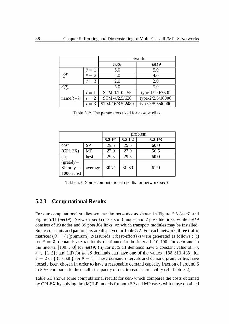
88 Chapter 5: Routing and Dimensioning of Multi-Class IP/MPLS Networks
networknet6 net19
θ = 1 5.0 5.0cOPθ θ = 2 4.0 4.0
θ = 3 2.0 2.0cOPaggr 5.0 5.0
t = 1 STM-1/1.0/155 type-1/1.0/2500name/ξt/kt t = 2 STM-4/2.5/620 type-2/2.5/10000
t = 3 STM-16/8.5/2480 type-3/8.5/40000
Table 5.2: The parameters used for case studies
problem5.2-P1 5.2-P2 5.2-P3
cost SP 29.5 29.5 60.0(CPLEX) MP 27.0 27.0 56.5cost best 29.5 29.5 60.0(greedy−SP only− average 30.71 30.69 61.91000 runs)
Table 5.3: Some computational results for networknet6
5.2.3 Computational Results
For our computational studies we use the networks as shown in Figure 5.8 (net6) andFigure 5.11 (net19). Networknet6consists of 6 nodes and 7 possible links, whilenet19consists of 19 nodes and 35 possible links, on which transport modules may be installed.Some constants and parameters are displayed in Table 5.2. For each network, three trafficmatrices (Θ = 1(premium), 2(assured), 3(best-effort)) were generated as follows : (i)for θ = 3, demands are randomly distributed in the interval[10, 100] for net6 and inthe interval[100, 500] for net19; (ii) for net6all demands have a constant value of50,θ ∈ 1, 2; and (iii) for net19demands can have one of the values155, 310, 465 forθ = 2 or 310, 620 for θ = 1. These demand intervals and demand granularities haveloosely been chosen in order to have a reasonable demand capacity fraction of around 5to 50% compared to the smallest capacity of one transmission facility (cf. Table 5.2).
Table 5.3 shows some computational results fornet6which compares the costs obtainedby CPLEX by solving the (M)ILP models for both SP and MP cases with those obtained

5.2: Network Dimensioning 89
[190.5,193.5) [196.5,199.5) [202.5,209)0
10
20
30
Cost Distribution
Occ
uran
ce (
%)
type−1 type−2 type−30
20
40
60Installed Transport Modules
Tot
al In
stal
led
[188,191) [194,197) [200,205)0
10
20
30
Occ
uran
ce (
%)
type−1 type−2 type−30
20
40
60
Tot
al In
stal
led
[453.5,459.5) [465.5,471.5) [477.5,490)0
10
20
30
40
Occ
uran
ce (
%)
Cost Intervaltype−1 type−2 type−3
0
20
40
60
Tot
al In
stal
led
Link Type
(a−i)
(a−ii)
(a−iii)
(b−i)
(b−ii)
(b−iii)
Figure 5.12: Cost distribution and number of transport modules to be installed in networknet14for the cases (i)5.2-P1, (ii) 5.2-P2and (iii) 5.2-P3
by the proposed heuristic for 1000 iterations. Looking at the table, it is obvious that: (i)the multi-path (MP) routing strategy is cheaper than the single-path (SP) case for all prob-lems; (ii) a routing scheme based on aggregate can offer the same optimal solution withrespect to the network cost as that offered by a per-class routing scheme; (iii) deployingper-aggregate OP constraints as in5.2-P3can be more expensive than deploying per-classOP constraints as in5.2-P1and5.2-P2; and (iv) for networknet6the heuristic performswell in the sense that it can find the optimal solutions and the differences between theaverage to the optimal costs in all cases are below the value of 5%.
Table 5.4 shows the results for networknet19. CPLEX was configured to terminate ifeither thegap2 is less than 1% or the computation time of 15 hours is reached. As in-dicated by the gap values in the CPLEX column, the last termination criterion is always
2A gap is the distance between the current best feasible solution and a possible lower-bound value. Itsvalue can be used by CPLEX as a termination criterion.

90 Chapter 5: Routing and Dimensioning of Multi-Class IP/MPLS Networks
CPLEX greedycost gap(%) (best cost of 100 runs)
problem 5.2-P1 165.5 6.18 190.5(SP only) 5.2-P2 166.5 4.19 188.0
5.2-P3 423.5 3.48 453.5
Table 5.4: Results for networknet19
used for all problems. The greedy heuristic was called 100 times for each problem whichcorresponds to a computation time of less than 2 minutes. The costs of the best solutionresulting from the greedy heuristic are shown in the last column in the table. The bestresult from the greedy heuristic is up to 15% worse than the result from the ILP approach.However, the ILP approach needs significantly longer computing time.
Figures 5.12a show the cost distribution resulting from the heuristic applied tonet19for100 iterations for the case5.2-P1(a-i), 5.2-P2(a-ii) and5.2-P3(a-iii). As can be seen inthe figures, the solutions for5.2-P3in this case are also much more expensive comparedto 5.2-P1and5.2-P2. Furthermore, it seems that the heuristic performs better if we deployper-aggregate routing (5.2-P2) than per-class routing (5.2-P1): the best and mean cost for5.12a-ii of188 and197.29 is better than that of190.5 and197.81 for 5.12a-i. Figures5.12b give the number of transport modules to be installed in the network for the bestsolution found by the heuristic. The number of transport modules to be installed in5.2-P1and5.2-P2differ only in an additionaltype-2module, which is also indirectly expressedby the cost difference of2.5. As the capacity requirements grow, e.g. in order to fulfillthe aggregate OP constraints in5.2-P3case, transport modules of higher capacity aremore beneficial (cf. the cost and capacity parameters in Table 5.2). This can be seen bycomparing 5.12b-iii to 5.12b-ii and 5.12b-i.
Finally, Figure 5.13 displays link utilization and OP factors for all traffic classes for thebest solution in5.2-P2case i.e. the configuration with the number of installed transportmodules as shown in Figure 5.12b-ii. The minimum aggregate OP factor is about1.7which corresponds to maximum utilization of about60%. The values ofλθmin for eachθ are(5.04; 4.00; 2.92) and thus satisfy the requirements of the minimum valuescOP
θ of(5.0; 4.0; 2.0). The minimum utilization forθ = 3 is about4%, which happens on linknumbered by 22. This explains the high value of the OP factor forθ = 3 in Figure 5.13dfor the corresponding link.
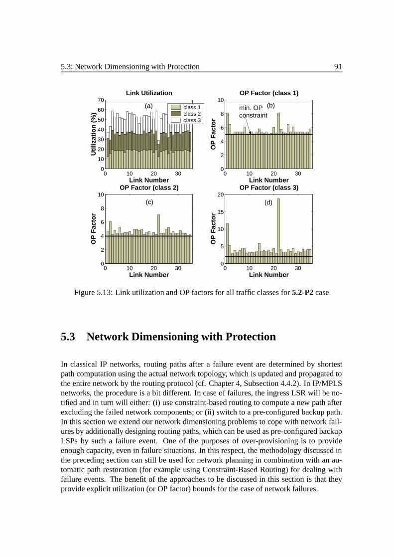
5.3: Network Dimensioning with Protection 91
0 10 20 300
10
20
30
40
50
60
70
Link Number
Util
izat
ion
(%)
Link Utilization
class 1class 2class 3
0 10 20 300
2
4
6
8
10OP Factor (class 1)
OP
Fac
tor
Link Number
0 10 20 300
2
4
6
8
10OP Factor (class 2)
OP
Fac
tor
Link Number0 10 20 30
0
5
10
15
20OP Factor (class 3)
OP
Fac
tor
Link Number
(a) (b)
(c) (d)
min. OP constraint
Figure 5.13: Link utilization and OP factors for all traffic classes for5.2-P2case
5.3 Network Dimensioning with Protection
In classical IP networks, routing paths after a failure event are determined by shortestpath computation using the actual network topology, which is updated and propagated tothe entire network by the routing protocol (cf. Chapter 4, Subsection 4.4.2). In IP/MPLSnetworks, the procedure is a bit different. In case of failures, the ingress LSR will be no-tified and in turn will either: (i) use constraint-based routing to compute a new path afterexcluding the failed network components; or (ii) switch to a pre-configured backup path.In this section we extend our network dimensioning problems to cope with network fail-ures by additionally designing routing paths, which can be used as pre-configured backupLSPs by such a failure event. One of the purposes of over-provisioning is to provideenough capacity, even in failure situations. In this respect, the methodology discussed inthe preceding section can still be used for network planning in combination with an au-tomatic path restoration (for example using Constraint-Based Routing) for dealing withfailure events. The benefit of the approaches to be discussed in this section is that theyprovide explicit utilization (or OP factor) bounds for the case of network failures.

92 Chapter 5: Routing and Dimensioning of Multi-Class IP/MPLS Networks
(c) (d) (e) (f)
(a) (b)
1
3 4
21
3
1 2
3 4
21
3 443
1 2
43
1 2
Normal
Backup
2
4
Figure 5.14: Routing paths in case of single-link failures
Let us look at a small network with a normal and a backup LSP as displayed in Figures5.14a and 5.14b. Note, that here we only consider: (i) two demands, namely those be-tween node pairs(1, 4) and(3, 4); (ii) single-link failures. The normal LSP for node pair(1, 4) will fail if the link (1, 2) or link (2, 4) fails (Figures 5.14c and 5.14e). In these cases,the backup LSP is used for routing. Analogously, the backup LSP for node pair(3, 4) isused if link (3, 4) fails (Figures 5.14f). By contrast, as can be seen from Figures 5.14d,the backup LSPs are not activated if link(1, 3) fails, since it is not used by the normalrouting paths. For all single-link failure scenarios above, the backup LSPs are not activesimultaneously. For example, if we look at link(1, 3), it is only occupied by one backupLSP at a time (Figures 5.14c, 5.14e and 5.14f). This means, that the capacity on link(1, 3)can besharedby both backup LSPs. In the literature, such a way of providing backuppaths is known asshared protectionas opposed todedicated protection3, where capacityfor each backup path can not be shared and must be provided in a dedicated manner.
5.3.1 Mathematical Models
Table 5.5 lists some additional notations needed for extending the formulation in Subsec-tion 5.2.1. For simultaneously planning backup LSPs, the formulation5.2-P1 is trans-formed to the following problem (denoted by5.3-P1).
3It is sometimes also calledhot-stand-byor 1+1 protection.
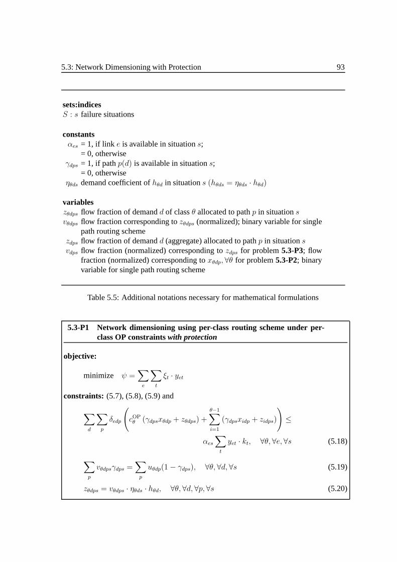
5.3: Network Dimensioning with Protection 93
sets:indicesS : s failure situations
constantsαes = 1, if link e is available in situations;
= 0, otherwiseγdps = 1, if pathp(d) is available in situations;
= 0, otherwiseηθds demand coefficient ofhθd in situations (hθds = ηθds · hθd)
variableszθdps flow fraction of demandd of classθ allocated to pathp in situationsvθdps flow fraction corresponding tozθdps (normalized); binary variable for single
path routing schemezdps flow fraction of demandd (aggregate) allocated to pathp in situationsvdps flow fraction (normalized) corresponding tozdps for problem5.3-P3; flow
fraction (normalized) corresponding toxθdp, ∀θ for problem5.3-P2; binaryvariable for single path routing scheme
Table 5.5: Additional notations necessary for mathematical formulations
5.3-P1 Network dimensioning using per-class routing scheme under per-class OP constraintswith protection
objective:
minimize ψ =∑e
∑t
ξt · yet
constraints: (5.7), (5.8), (5.9) and
∑d
∑p
δedp
(cOPθ (γdpsxθdp + zθdps) +
θ−1∑i=1
(γdpsxidp + zidps)
)≤
αes∑t
yet · kt, ∀θ, ∀e, ∀s (5.18)
∑p
vθdpsγdps =∑p
uθdp(1− γdps), ∀θ, ∀d, ∀s (5.19)
zθdps = vθdps · ηθds · hθd, ∀θ, ∀d, ∀p, ∀s (5.20)

94 Chapter 5: Routing and Dimensioning of Multi-Class IP/MPLS Networks
Inequality (5.18) is obtained by replacingxθdp in (5.7) by(γdpsxθdp + zθdps), which canbe interpreted as the total of the normal flow, which isstill available in case of failures(expressed byγdpsxθdp) and the backup flow, which may be activated in case of failures (expressed byzθdps). Furthermore, the constantαes at the right side, will force theflow variableszθdps to be zero if the corresponding link fails. Equation (5.19) ensuresthat the fraction of recovered traffic is exactly the same as that of the normal traffic,which is affected by the failure. Equation (5.20) gives the definition of the amount ofadditional flowzθdps as the multiplication of fractional variablevθdps and demand volumehθd in situations. Looking at inequalities (5.19) and (5.8), it is obvious that the pathcandidate list for a certain demandd should have at least two paths, which are link-disjoint; otherwise5.3-P1would be infeasible.
Furthermore, using per-aggregate routing scheme, the problem of network dimensioningwith LSP protection under per-class OP constraints (denoted by5.3-P2), can be expressedas follows.
5.3-P2 Network dimensioning usingper-aggregate routing scheme underper-class OP constraintswith protection
objective:
minimize ψ =∑e
∑t
ξt · yet
constraints: (5.7), (5.10), (5.11), (5.18) and∑p
vdpsγdps =∑p
udp(1− γdps), ∀d, ∀s (5.21)
zθdps = vdps · ηθds · hθd, ∀θ, ∀d, ∀p, ∀s (5.22)
Different from5.3-P1, in 5.3-P2we use aggregate routing variableudp andvdps. Lastly,the problem under per-aggregate OP constraints (denoted by5.3-P3) can be written as:
5.3-P3 Network dimensioning usingper-aggregate routing scheme underper-aggregate OP constraintswith protection
objective:
minimize ψ =∑e
∑t
ξt · yet
constraints: (5.10), (5.12), (5.13), (5.21) and

5.3: Network Dimensioning with Protection 95
cOPaggr
∑d
∑p
δedp (γdpsxdp + zdps) ≤ αes∑t
yet · kt, ∀e, ∀s (5.23)
zdps = vdps∑θ
ηθdshθd, ∀d, ∀p, ∀s (5.24)
Note, that the constantscOPθ andcOP
aggr for a failure event in (5.18) and (5.23) can be setdifferently from those for normal operation in (5.7) and (5.12).
5.3.2 Solving with Heuristics
The algorithm ALG-1 presented in Section 5.2.2 can also be extended to simultaneouslyplan backup LSPs. The first possibility is depicted in Figure 5.15. The main differencesfrom ALG-1 can be seen at the loop process marked by L4, while the rest of the algorithmis almost identical. For each normal pathp ∈ P (θ, d), there is a set of backup pathcandidatesQ(θ, d, p). The incremental cost is thus computed as a function of a possibleassignment of demandhθd to normal pathp and backup pathq ∈ Q(θ, d, p). Compared toALG-1, the time needed for computation of∆ψ(p, q, e)4 is multiplied by|S| if e ∈ q. Thisis implicitly indicated in the example in Figure 5.14 : in order to decide how many backupcapacities have to be provided on link(1, 3), we have to consider all failure situations.Thus, the time necessary (i) for computing∆ψ(p, q) is multiplied by a factor|S| · lq ,wherelq is the number of links contained in the backup pathq; and (ii) for the overallprocess is multiplied by|Q|av · |S| · lav, where|Q|av is the average number of backup pathcandidates andlav is the average number of links on a backup path. That is, if for ALG-1we need about 5 seconds using networknet19(see Figure 5.11 and Subsection 5.2.3), withsingle-link failures scenario we need around 25 minutes for ALG-2 in a single algorithmexecution5. Since such a greedy heuristic will be used in combination with a stochasticsearch method, which typically requires more than 100 iterations, ALG-2 is less attractivecompared to the linear programming approach with limited execution time (say 10 to 15hours).
The second possibility is displayed in Figure 5.16 and denoted by ALG-3. In this case,for each normal path candidatep ∈ P1(θ, d) there is only one backup path candidateq ∈ P2(θ, d). The pair of pathp andq is pre-computed and put at the same position inthe listsP1(θ, d) andP2(θ, d). Now, compared to ALG-1, execution time of the overallprocess is multiplied by|S| · lav. In our previous example, this corresponds to around 10
4The incremental cost for an assignment of normal pathp and backup pathq on a certain linke.5It is assumed that the average number of: (i) backup paths in the lists is about 3; and (ii) links on backup
paths is also around 3.
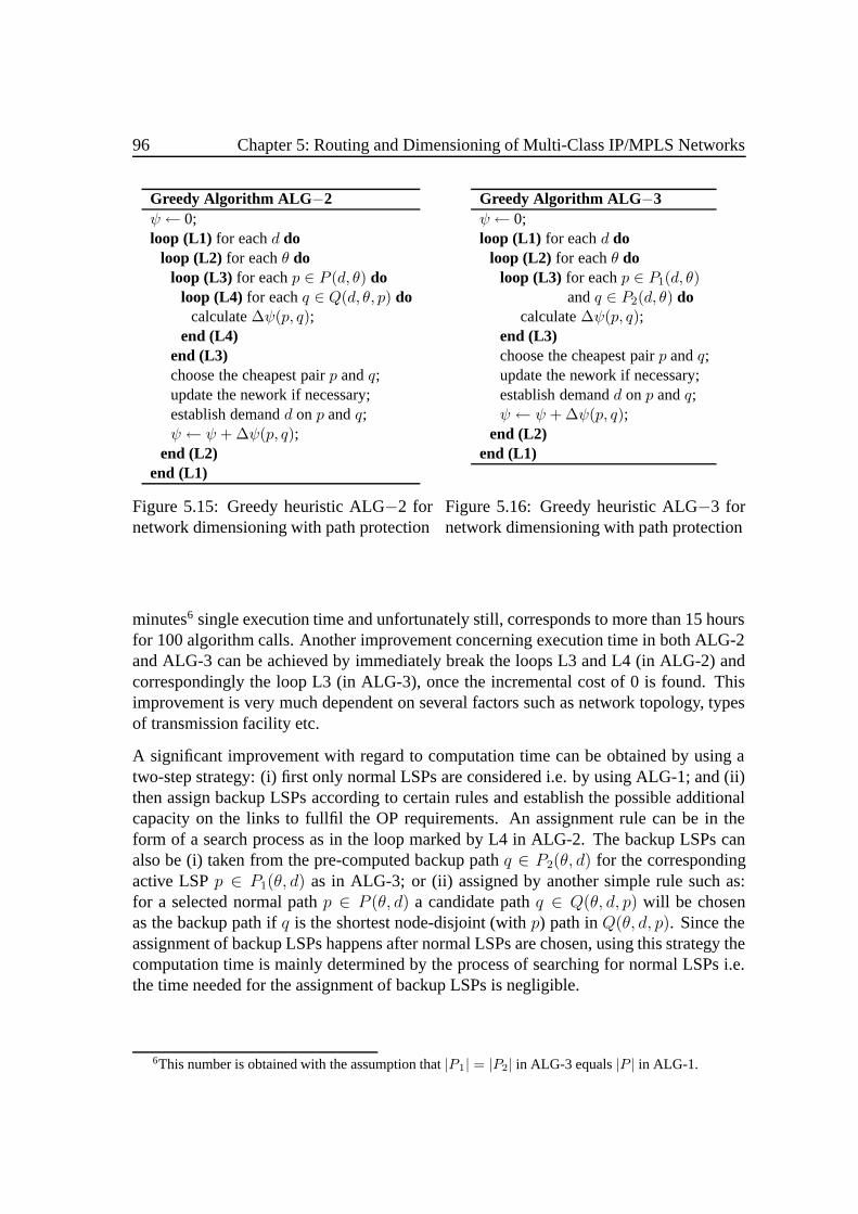
96 Chapter 5: Routing and Dimensioning of Multi-Class IP/MPLS Networks
Greedy Algorithm ALG −2ψ← 0;loop (L1) for eachd do
loop (L2) for eachθ doloop (L3) for eachp ∈ P (d, θ) do
loop (L4) for eachq ∈ Q(d, θ, p) docalculate∆ψ(p, q);
end (L4)end (L3)choose the cheapest pairp andq;update the nework if necessary;establish demandd on p andq;ψ ← ψ + ∆ψ(p, q);
end (L2)end (L1)
Figure 5.15: Greedy heuristic ALG−2 fornetwork dimensioning with path protection
Greedy Algorithm ALG −3ψ← 0;loop (L1) for eachd do
loop (L2) for eachθ doloop (L3) for eachp ∈ P1(d, θ)
andq ∈ P2(d, θ) docalculate∆ψ(p, q);
end (L3)choose the cheapest pairp andq;update the nework if necessary;establish demandd onp andq;ψ ← ψ + ∆ψ(p, q);
end (L2)end (L1)
Figure 5.16: Greedy heuristic ALG−3 fornetwork dimensioning with path protection
minutes6 single execution time and unfortunately still, corresponds to more than 15 hoursfor 100 algorithm calls. Another improvement concerning execution time in both ALG-2and ALG-3 can be achieved by immediately break the loops L3 and L4 (in ALG-2) andcorrespondingly the loop L3 (in ALG-3), once the incremental cost of 0 is found. Thisimprovement is very much dependent on several factors such as network topology, typesof transmission facility etc.
A significant improvement with regard to computation time can be obtained by using atwo-step strategy: (i) first only normal LSPs are considered i.e. by using ALG-1; and (ii)then assign backup LSPs according to certain rules and establish the possible additionalcapacity on the links to fullfil the OP requirements. An assignment rule can be in theform of a search process as in the loop marked by L4 in ALG-2. The backup LSPs canalso be (i) taken from the pre-computed backup pathq ∈ P2(θ, d) for the correspondingactive LSPp ∈ P1(θ, d) as in ALG-3; or (ii) assigned by another simple rule such as:for a selected normal pathp ∈ P (θ, d) a candidate pathq ∈ Q(θ, d, p) will be chosenas the backup path ifq is the shortest node-disjoint (withp) path inQ(θ, d, p). Since theassignment of backup LSPs happens after normal LSPs are chosen, using this strategy thecomputation time is mainly determined by the process of searching for normal LSPs i.e.the time needed for the assignment of backup LSPs is negligible.
6This number is obtained with the assumption that|P1| = |P2| in ALG-3 equals|P | in ALG-1.

5.4: LSP Design for Multi-Class IP/MPLS Networks 97
CPLEX greedycost gap(%) (best cost of 100 runs)
problem 5.3-P1 268.5 9.93 310.5(SP only) 5.3-P2 268.5 9.47 303.5
5.3-P3 688 3.75 755
Table 5.6: Results for networknet19, considering backup LSPs
5.3.3 Comparison
Table 5.6 shows the numerical results for networknet19. As in Subsection 5.2.3 CPLEXwas configured to terminate if either the gap is less than 1% or the computation timeof 15 hours is reached. The heuristic is applied in a two-step strategy as mentioned inthe preceding subsection: first normal LSPs will be determined using ALG-1 and thenbackup LSPs are assigned to the corresponding normal LSPs using a minimum-hop andnode-disjoint criterion. With this strategy, the time needed for computation is less than 5minutes. The costs of the best solutions resulting from the heuristic are shown in the lastcolumn in the table. In this case, the best result from the greedy heuristic is up to 16%worse than the result from the ILP approach. Regarding the cost for a certain problem, thevalues in Table 5.6 are roughly higher by the factor of 1.6 compared to those in Table 5.4,both for CPLEX and heuristic results. These additional costs are necessary for providingenough resources in the networks in order to fulfill the OP requirements in the case ofsingle-link failures.
5.4 LSP Design for Multi-Class IP/MPLS Networks
In the last two sections, we have focused on network dimensioning i.e. on the problemhow many and which type of transmission facility has to be provided for each link. Us-ing the knowledge gathered so far, we will close this chapter by presenting several ideason LSP design for multi-class IP/MPLS networks. But different from the approach inSection 5.1, here it is assumed, that routing is entirely performed by ER-LSPs. In Chap-ter 4, Subsections 4.1.1 and 4.4.1, two mathematical models for the routing problem areintroduced (GRP and SPRP). Though in the preceding chapter they were intended forcomparison purposes with shortest path routing, they can be realized in IP/MPLS net-works. In this section, we will extend these models, supporting per-class traffic matricesand over-provisioning constraints. The problem of LSP design in multi-class IP/MPLSnetworks under over-provisioning constraints (denoted by5.4-P1) can be expressed asfollows:
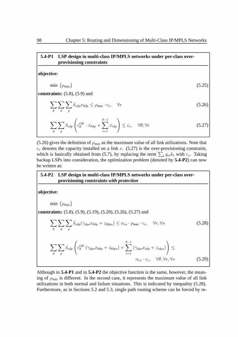
98 Chapter 5: Routing and Dimensioning of Multi-Class IP/MPLS Networks
5.4-P1 LSP design in multi-class IP/MPLS networks under per-class over-provisioning constraints
objective:
min ρmax (5.25)
constraints: (5.8), (5.9) and∑θ
∑d
∑p
δedpxθdp ≤ ρmax · ce, ∀e (5.26)
∑d
∑p
δedp
(cOPθ · xθdp +
θ−1∑i=1
xidp
)≤ ce, ∀θ, ∀e (5.27)
(5.26) gives the definition ofρmax as the maximum value of all link utilizations. Note thatce denotes the capacity installed on a linke. (5.27) is the over-provisioning constraint,which is basically obtained from (5.7), by replacing the term
∑t yetkt with ce. Taking
backup LSPs into consideration, the optimization problem (denoted by5.4-P2) can nowbe written as:
5.4-P2 LSP design in multi-class IP/MPLS networks under per-class over-provisioning constraints with protection
objective:
min ρmaxconstraints: (5.8), (5.9), (5.19), (5.20), (5.26), (5.27) and∑
θ
∑d
∑p
δedp(γdpsxθdp + zθdps) ≤ αes · ρmax · ce, ∀e, ∀s (5.28)
∑d
∑p
δedp
(cOPθ (γdpsxθdp + zθdps) +
θ−1∑i=1
(γdpsxidp + zidps)
)≤
αes · ce, ∀θ, ∀e, ∀s (5.29)
Although in5.4-P1and in5.4-P2the objective function is the same, however, the mean-ing of ρmax is different. In the second case, it represents the maximum value of all linkutilizations in both normal and failure situations. This is indicated by inequality (5.28).Furthermore, as in Sections 5.2 and 5.3, single path routing scheme can be forced by re-
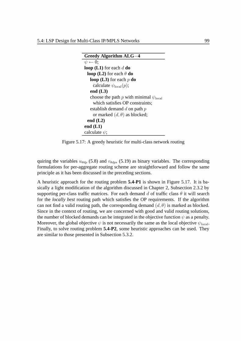
5.4: LSP Design for Multi-Class IP/MPLS Networks 99
Greedy Algorithm ALG −4ψ← 0;loop (L1) for eachd do
loop (L2) for eachθ doloop (L3) for eachp do
calculateψlocal(p);end (L3)choose the pathp with minimalψlocal
which satisfies OP constraints;establish demandd on pathp
or marked(d, θ) as blocked;end (L2)
end (L1)calculateψ;
Figure 5.17: A greedy heuristic for multi-class network routing
quiring the variablesuθdp (5.8) andvθdps (5.19) as binary variables. The correspondingformulations for per-aggregate routing scheme are straightforward and follow the sameprinciple as it has been discussed in the preceding sections.
A heuristic approach for the routing problem5.4-P1 is shown in Figure 5.17. It is ba-sically a light modification of the algorithm discussed in Chapter 2, Subsection 2.3.2 bysupporting per-class traffic matrices. For each demandd of traffic classθ it will searchfor the locally bestrouting path which satisfies the OP requirements. If the algorithmcan not find a valid routing path, the corresponding demand(d, θ) is marked as blocked.Since in the context of routing, we are concerned with good and valid routing solutions,the number of blocked demands can be integrated in the objective functionψ as a penalty.Moreover, the global objectiveψ is not necessarily the same as the local objectiveψlocal.Finally, to solve routing problem5.4-P2, some heuristic approaches can be used. Theyare similar to those presented in Subsection 5.3.2.

100 Chapter 5: Routing and Dimensioning of Multi-Class IP/MPLS Networks
Chapter 6
Routing Optimization under DemandUncertainty
Till now, routing control is done by selecting paths in a way to optimize overall networkcost and performance based on agiventraffic matrix. Thus, quality of the resulting routingpattern is very dependent on the precision of the traffic matrix. Shift in traffic may resultin undesirable network performance and for a long-term time scale it may affect properoperation of the network. In the context of IP networks, trafficuncertaintyis becominga more and more important issue due to considerable growth rates in terms of both sizeand number of different services, which in turn make precise forecast of traffic demandsvery difficult. From network operators’ point of view, it may be desirable having a rout-ing configuration which is sufficiently flexible to capture certain traffic variations, whilekeeping resource utilization as efficient as possible.
This chapter is devoted to routing optimization under demand uncertainty in order to copewith such situations. Some novel aspects and our scientific contributions are as follows:
• We propose several traffic uncertainty models based on simple outbound/inboundtraffic constraints. A more flexible model addressing the case where traffic is par-tially uncertain, is also introduced.
• We present the formulae for computing a worst case load that can happen on a linkfor the corresponding traffic uncertainty models.
• We show that our traffic engineering approaches developed in Chapter 4 can alsobe used to control routing under such demand conditions.
In the next section, we first address routing optimization for the basic asymmetrical de-mand models, while symmetrical models are presented in Section 6.2. A more flexible
101
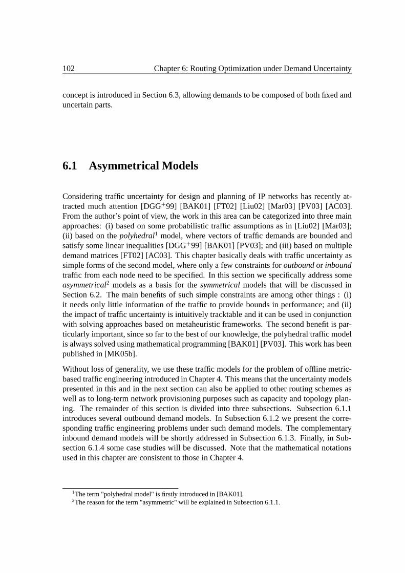
102 Chapter 6: Routing Optimization under Demand Uncertainty
concept is introduced in Section 6.3, allowing demands to be composed of both fixed anduncertain parts.
6.1 Asymmetrical Models
Considering traffic uncertainty for design and planning of IP networks has recently at-tracted much attention [DGG+99] [BAK01] [FT02] [Liu02] [Mar03] [PV03] [AC03].From the author’s point of view, the work in this area can be categorized into three mainapproaches: (i) based on some probabilistic traffic assumptions as in [Liu02] [Mar03];(ii) based on thepolyhedral1 model, where vectors of traffic demands are bounded andsatisfy some linear inequalities [DGG+99] [BAK01] [PV03]; and (iii) based on multipledemand matrices [FT02] [AC03]. This chapter basically deals with traffic uncertainty assimple forms of the second model, where only a few constraints foroutboundor inboundtraffic from each node need to be specified. In this section we specifically address someasymmetrical2 models as a basis for thesymmetricalmodels that will be discussed inSection 6.2. The main benefits of such simple constraints are among other things : (i)it needs only little information of the traffic to provide bounds in performance; and (ii)the impact of traffic uncertainty is intuitively tracktable and it can be used in conjunctionwith solving approaches based on metaheuristic frameworks. The second benefit is par-ticularly important, since so far to the best of our knowledge, the polyhedral traffic modelis always solved using mathematical programming [BAK01] [PV03]. This work has beenpublished in [MK05b].
Without loss of generality, we use these traffic models for the problem of offline metric-based traffic engineering introduced in Chapter 4. This means that the uncertainty modelspresented in this and in the next section can also be applied to other routing schemes aswell as to long-term network provisioning purposes such as capacity and topology plan-ing. The remainder of this section is divided into three subsections. Subsection 6.1.1introduces several outbound demand models. In Subsection 6.1.2 we present the corre-sponding traffic engineering problems under such demand models. The complementaryinbound demand models will be shortly addressed in Subsection 6.1.3. Finally, in Sub-section 6.1.4 some case studies will be discussed. Note that the mathematical notationsused in this chapter are consistent to those in Chapter 4.
1The term "polyhedral model" is firstly introduced in [BAK01].2The reason for the term "asymmetric" will be explained in Subsection 6.1.1.

6.1: Asymmetrical Models 103
6.1.1 Outbound Demand Models
Using explicit modeling for demand uncertainty generally means that the traffic matrixF = (fu,v), u = v ∈ N may vary over time, while still satisfying specific constraints.Here we focus onoutboundtraffic, where the term "outbound" is used to point to trafficoriginating from a certain node. Iff u,v denotes the demand to be carried from sourceuto destinationv, the basic outbound demand model can be expressed as:∑
v∈Nfu,v ≤ fuout (6.1)
wherefuout gives the maximum outbound traffic at nodeu. It is obvious that (6.1) allowsan individual flowf u,v to vary over time as long as the flow aggregate
∑v∈N f
u,v is lessthan the maximum valuef uout. Furthermore, (6.1) also indicates that providing minimalinformation about maximum aggregate trafficf uout will result in a highlyasymmetricsit-uation since the terminating traffic at each nodev is upper-bounded by
∑t∈N f
tout; v = t.
To indirectly limit the terminating traffic at each node, we can additionally provide a sec-ond parameterϕuout ≤ fuout as the maximum capacity that can be occupied by a singleflow, which corresponds to a certain node pair. That is
fu,v ≤ ϕuout ; ∀v (6.2)
Using this constraint we upperbound the terminating traffic at nodev by the value of∑t∈N ϕ
tout; v = t or ϕ · (|N | − 1) for the case ofϕuout = ϕ, ∀u.
The second possibility to indirectly limit the terminating trafffic at each node is togener-alize(6.1). LetΩu
r be defined as a set of destination nodes belonging to groupr for trafficoriginating fromu, where∪rΩu
r = N \u andΩur ∩Ωu
s = ∅, s = r. For each nodeu andΩur , we specify a maximum outbound trafficf ur,out. Thus, (6.1) can now be written as:
∑v∈Ωu
r
fu,v ≤ fur,out (6.3)
In this case, the terminating traffic atv is upperbounded by∑
t∈N∑
r ftr,out·δt,vr , whereδt,vr
having the value of 1 ifΩtr containsv, and 0 otherwise.Generalizationcan also be made
for (6.2) by specifying the maximum flow to different groups of nodesϕur,out ≤ fur,out.In this case (6.2) is replaced by (6.4). The terminating traffic atv is now limited by∑
t∈N∑
r ϕtr,out · δt,vr .
fu,v ≤ ϕur,out ; ∀v ∈ Ωur (6.4)
Table 6.1 summarizes all possible uncertainty models with the traffic constraints that haveto be satisfied, including those that will be addressed in Section 6.2.

104 Chapter 6: Routing Optimization under Demand Uncertainty
Model Model Notation (m) Constraintsoutbound M1 (6.1)inbound M2 (6.13)outbound +max-flow M3 (6.1)(6.2)inbound +max-flow M4 (6.13)(6.14)hose M5 (6.1)(6.13)hose +max-flow M6 (6.1)(6.2)(6.13)(6.14)
outbound +group M7 (6.3)inbound +group M8 (6.15)outbound +max-flow+ group M9 (6.3)(6.4)inbound +max-flow+ group M10 (6.15)(6.16)hose +group M11 (6.3)(6.15)hose +max-flow+ group M12 (6.3)(6.4)(6.15)(6.16)
Table 6.1: Several demand uncertainty models
6.1.2 Traffic Engineering under Outbound Traffic Constraints
For agiventraffic matrix, metric-based traffic engineering approaches, will try to find aset of metric values (a weight-system) that optimizes performance e.g. with respect tonetwork utilization. Here, we consider the problem of metric-based traffic engineeringfor uncertain demands, which satify severaloutboundtraffic constraints, for both multi-path and unique single-path routing strategies (cf. Section 4.1). However, the formulationbelow is generic and remains the same for all models in Table 6.1. One exception isthe calculation of link loads, which is unique for each demand model. Since here weconsider uncertain demands, the terms "load" and "utilization" will always refer to loadand utilization in the worst case i.e. theupper-bound values. Sometimes, for the samereason we also use the term "capacity occupancy" instead of "utilization". Basically,the optimization problem of metric-based traffic engineering for uncertain demands isidentical to (4.5)−(4.6) by interpreting utilizationρi,j as mentioned before. For clarity,we display again the formulation below. This will be referred to as problem6.1-P1.
6.1-P1 Generic formulation for metric-based traffic engineering,minimiz-ing maximum utilization
min ρmax (6.5)
ρi,j ≤ ρmax ; ∀(i, j) ∈ A (6.6)

6.1: Asymmetrical Models 105
Furthermore, for comparison it might be of interest to maximize theuniform outboundtraffic i.e. fuout = f c, ∀u ∈ N . Given the maximum allowable link utilizationρcmax, thisproblem variant (denoted by6.1-P2) can be expressed as follows:
6.1-P2 Generic formulation for metric-based traffic engineering,maximiz-ing uniform outbound traffic
max f c (6.7)
ρi,j ≤ ρcmax ; ∀(i, j) ∈ A (6.8)
Note that both6.1-P1and 6.1-P2 are generic irrespective of any explicit relationshipbetweenρi,j (or link loadli,j) and demands (or demand models).
In the following we will derive the formulae for the outbound models (M1,M3,M7,M9).The corresponding formulae for the inbound models (M2,M4,M8,M10) and for the sym-metrical models (M5,M6,M11,M12) will be addressed in Subsection 6.1.3 and in Sec-tion 6.2, respectively.
Calculating Link Loads
Figure 6.1a shows a small network and the corresponding metric value for each link,Figure 6.1b several routing paths for traffic originating from node1, and Figure 6.1c theresulting maximum load fraction on the links affected by uncertain traffic from node1(to be explained below). Setting the metric values homogeneously causes split of trafficdestined to node4 and6 as shown in Figure 6.1b, while traffic to the rest of the nodes isnot split and follows the paths(1−2), (1−3) and(1−3−5), respectively. Thus the link(1, 3) for instance, is occupied by four different flows i.e. those destined to nodes3, 4, 5and6 with theper-flowtraffic portion of100%, 50%, 100% and50%, respectively. Sincetraffic is considered as uncertain and we are given only the maximum aggregate trafficvalues (as expressed by inequality (6.1)), a single flow in theworstcase can occupy thewhole resources allocated for traffic aggregate. In the above example, it means: (i)100%of the total traffic originated from node1 could occupy the link(1, 3) for for the caseswhere the traffic aggregate is assigned entirely to the flow terminating at nodes3 or 5; (ii)50% of the total traffic originated from node1 could occupy the link(3, 4) for the casewhere the traffic aggregate is assigned entirely to the flow terminating at node4; etc.
Let lui,j(M1) be a real variable associated with the load on link(i, j) resulting from flowaggregatefuout originating from nodeu for uncertainty model M1. From our previousexample, it is clear thatlui,j(M1) shall be the multiplication of the flow aggregatef uout and

106 Chapter 6: Routing Optimization under Demand Uncertainty
1
1
1
1
1
(c)
1
1
link weights per−source fractions(source = node 1)per−flow fractions
(source = node 1)
1
0.51
1 0.75
1 2
3 4
5 60.25
1 2
3 4
5 60.25
0.25 0.5
0.5
0.5 0.5
(a) (b)
65
43
2
1
Figure 6.1: An example of routing demands using the ECMP rule for calculating loadupper-bounds in theoutboundmodel
the maximum traffic fractionβu,vi,j for all individual flows originating fromu. That is:
lui,j(M1) = fuout ·maxv∈N
βu,vi,j (6.9)
Using a similar intuitive method, the following equations for uncertainty models M3, M7and M9 can be easily derived.
lui,j(M3) = min(fuout ·maxv∈N
βu,vi,j , ϕuout ·
∑v∈N
βu,vi,j ) (6.10)
lui,j(M7) =∑r
(fur,out ·maxv∈Ωu
r
βu,vi,j ) (6.11)
lui,j(M9) =∑r
min(fur,out ·maxv∈Ωu
r
βu,vi,j , ϕur,out ·
∑v∈Ωu
r
βu,vi,j ) (6.12)
The total load on a link(i, j) for uncertainty modelm, denoted byli,j(m), is the summa-tion of the loads contributed by all nodes i.e.:
li,j(m) =∑u
lui,j(m) (6.13)
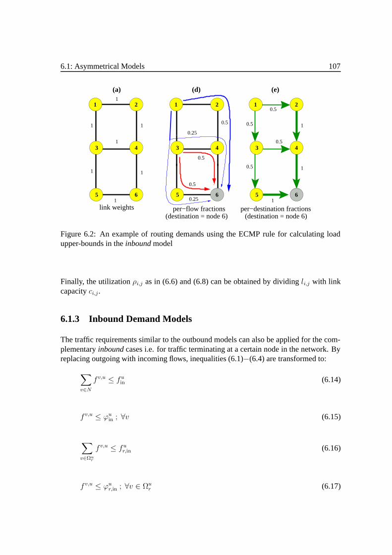
6.1: Asymmetrical Models 107
1
1
1
1
1
1 1
1
0.5
link weights
(a) (d) (e)
1 2
3 4
5 60.25
0.5
0.5
0.25
per−flow fractions(destination = node 6)
1
0.5
1 2
3 4
5 61
10.5
0.5
(destination = node 6)per−destination fractions
65
43
2
0.5
Figure 6.2: An example of routing demands using the ECMP rule for calculating loadupper-bounds in theinboundmodel
Finally, the utilizationρi,j as in (6.6) and (6.8) can be obtained by dividingli,j with linkcapacityci,j.
6.1.3 Inbound Demand Models
The traffic requirements similar to the outbound models can also be applied for the com-plementaryinboundcases i.e. for traffic terminating at a certain node in the network. Byreplacing outgoing with incoming flows, inequalities (6.1)−(6.4) are transformed to:
∑v∈N
f v,u ≤ fuin (6.14)
f v,u ≤ ϕuin ; ∀v (6.15)
∑v∈Ωu
r
f v,u ≤ fur,in (6.16)
f v,u ≤ ϕur,in ; ∀v ∈ Ωur (6.17)
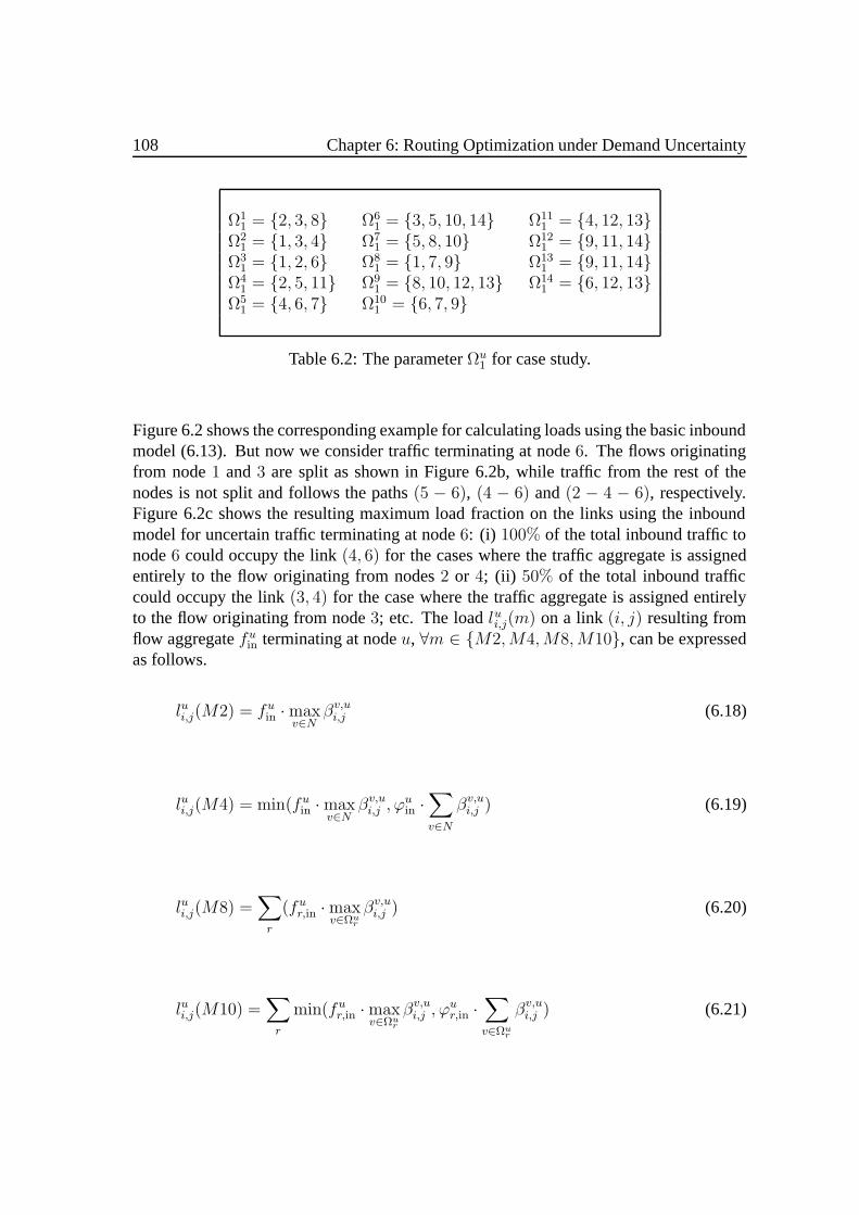
108 Chapter 6: Routing Optimization under Demand Uncertainty
Ω11 = 2, 3, 8 Ω6
1 = 3, 5, 10, 14 Ω111 = 4, 12, 13
Ω21 = 1, 3, 4 Ω7
1 = 5, 8, 10 Ω121 = 9, 11, 14
Ω31 = 1, 2, 6 Ω8
1 = 1, 7, 9 Ω131 = 9, 11, 14
Ω41 = 2, 5, 11 Ω9
1 = 8, 10, 12, 13 Ω141 = 6, 12, 13
Ω51 = 4, 6, 7 Ω10
1 = 6, 7, 9
Table 6.2: The parameterΩu1 for case study.
Figure 6.2 shows the corresponding example for calculating loads using the basic inboundmodel (6.13). But now we consider traffic terminating at node6. The flows originatingfrom node1 and3 are split as shown in Figure 6.2b, while traffic from the rest of thenodes is not split and follows the paths(5 − 6), (4 − 6) and(2 − 4 − 6), respectively.Figure 6.2c shows the resulting maximum load fraction on the links using the inboundmodel for uncertain traffic terminating at node6: (i) 100% of the total inbound traffic tonode6 could occupy the link(4, 6) for the cases where the traffic aggregate is assignedentirely to the flow originating from nodes2 or 4; (ii) 50% of the total inbound trafficcould occupy the link(3, 4) for the case where the traffic aggregate is assigned entirelyto the flow originating from node3; etc. The loadlui,j(m) on a link(i, j) resulting fromflow aggregatefuin terminating at nodeu, ∀m ∈ M2,M4,M8,M10, can be expressedas follows.
lui,j(M2) = fuin ·maxv∈N
βv,ui,j (6.18)
lui,j(M4) = min(fuin ·maxv∈N
βv,ui,j , ϕuin ·∑v∈N
βv,ui,j ) (6.19)
lui,j(M8) =∑r
(fur,in ·maxv∈Ωu
r
βv,ui,j ) (6.20)
lui,j(M10) =∑r
min(fur,in ·maxv∈Ωu
r
βv,ui,j , ϕur,in ·
∑v∈Ωu
r
βv,ui,j ) (6.21)

6.1: Asymmetrical Models 109
0 10 20 30 400
10
20
30
40
Link Number
Util
. Diff
eren
ce (
%)
Util. Difference relative to Util. of M3
M1
0 10 20 30 400
10
20
30
40
Link Number
Util
. Diff
eren
ce (
%)
Util. Difference relative to Util. of M7
M1
0 10 20 30 40
0
10
20
30
40
Link Number
Util
. Diff
eren
ce (
%)
Util. Difference relative to Util. of M3
M7
010
2030
40
0
5
10
Link Number
Util. Difference relative to Util. of M9
Util
. Diff
eren
ce (
%) M3
M7
(a) (b)
(c) (d)
Figure 6.3: Comparison of link utilization for different models using inverse capacitymetrics.
6.1.4 Case Study
Since both outbound and inbound models are asymmetric, here only outbound modelsare considered. For the following discussion we use networknet14as shown in Figure5.2, which consists of 14 nodes and 22 bidirectional links (each of 2.5 Gbps capacity).The maximum outbound demandf uout for uncertainty model M1 and M3 is set as follows:300 Mbps for nodes10, 13; 200 Mbps for nodes2, 6, 7, 9, 11, 14; and100 Mbps forthe rest of the nodes. For M7 and M9, destination nodesN \ u are classified to twodifferent groups (∀u), wherefu1,out = 0.6fuout andfu2,out = 0.4fuout. Table 6.2 shows theparameterΩu
1 for different nodesu andΩu2 is set asN \ (Ωu
1 ∪ u). The maximum flowϕuout for uncertainty model M3 as well asϕu1,out andϕu2,out for M9 is set homogeneouslyto the value of40 Mbps.

110 Chapter 6: Routing Optimization under Demand Uncertainty
Initial Network Utilization
Figure 6.3 shows theinitial network utilizations for the outbound models, resulting frominverse capacity metrics (denoted by InvCap), which in this case matches that resultingfrom unit metrics due to the homogeneity of link capacities. Knowing the link metrics, wecan compute the parameterβu,vi,j and in turn the corresponding link loads using the equa-tions (6.9)−(6.12). Figure 6.3a clearly indicates the benefit of inequality (6.2), by show-ing differences between link utilization calculated for M1 and for M3: the link utilizationfor M1 is much larger than that for M3. Figure 6.3b shows link utilization for uncertaintymodel M1 relative to that for M7 and signifies the benefit of (6.3). The maximum flowconstraint (6.2) and the general outbound traffic constraint (6.3) are not dominating eachother as displayed in Figure 6.3c. These constraints can also be applied simultaneouslyto achieve better network efficiency as illustrated in Figure 6.3d, which compares linkutilization for M3 and M7 relative to that of M9. Thus, concerning network usage, in oursample case uncertainty model M9 is the most efficient model while M1 the least efficientone; the efficiency of M3 and M7 is somewhere in-between. Generally, specifying moredemand information as maximum flow or outbound traffic to groups of nodes instead ofthat to a single group, can significantly save network resources, although this might alsoreduce the number of traffic variations being supported.
Figures 6.4a and 6.4b show link utilizations using InvCap metrics for uncertainty modelM1 (the last histogram in both graphs) compared to randomly generatedtraffic matri-ces, that do not violate the constraints3. Each histogram (except the last one) repre-sents maximum utilization on each link for 10 different traffic matrices. Thus in eachgraph we compare the utilization computed by (6.9) with 100 randomly generated traf-fic matrices. In Figure 6.4a all of the aggregate demandfu is carried by a single flowfu,v, u = v, while in Figure 6.4b each elementf u,v is randomly distributed in the interval[0, fu −∑v−1
t=1 fu,t]; u = t, u = v. Using both demand generation strategies, the value of
ρmax found in all experiments is always below 40% and the number of links that have uti-lizations which exactly match that resulting from M1 is below the value of 25%. This factsupports the asymmetric property of (6.1) that has been addressed in Subsection 6.1.1.
Optimization Results
Table 6.3 displays typical computation results with regard to some performance param-eters. It basically shows the optimization results both for6.1-P1and6.1-P2, comparedto the performance obtained by the original routing pattern. The last three columns indi-cate: the number of different flows carried by a link (ω link), the number of hops for a path(hpath) and the path delay (dpath), which is modeled statically and mainly determined by
3The load value for M1 is computed using Equ. (6.9), which is also used in the Figures 6.3a and 6.3b.By contrast, the load value for arandomlygenerated traffic matrix is calculated as usual using Equ. (4.1).

6.1: Asymmetrical Models 111
010
2030
40
0
20
40
60
Link Number
Comparison with 100 max. TMsU
tiliz
atio
n(%
)
010
2030
40
0
20
40
60
Link Number
Comparison with 100 random TMs
Util
izat
ion(
%)
M9 M7 M3 M1
20
30
40
50
60
Max. Utilization for Each ModelOptimization based on M1
Max
. Util
izat
ion
(%)
Model
InvCapMSP USP
M9 M7 M3 M1
20
30
40
50
60
Max. Utilization for Each ModelOptimization based on M3
Max
. Util
izat
ion
(%)
Model
InvCapMSP USP
(d)
(a) (b)
(c)
the last the last
Figure 6.4: Comparison of link utilization resulting from M1 and comparison of the max-imum utilization before and after optimization
propagation time.
Initially, using inverse capacity metrics, 56 flows are split and the maximum value ofρmax
for uncertainty model M1 is bounded by 57.6%. For the6.1-P1case, after optimizationit can be reduced to the value of 40.2% for multi shortest paths (MSP) case and corre-spondingly 44.2% for the unique shortest path (USP) case. Comparing the rows MSP andUSP, theprobability to obtain a better value ofρmax is something that can be taken forgranted, since the solution space for MSP is much larger than that for USP. In contrastto the general belief that splitting of traffic results in better utilization Table 6.3 indicatesthat low splitting values (rows 3 and 5) can go along with excellent maximum utilizationvalues. The average number of different flows carried by a link for the USP is lowerthan that for the MSP case. This can be seen as a logical impact of each routing strategy.The average values of the parameterhpath anddpath do not differ very much implying thatthe network topology provides flexibility for routing. The maximum utilization beforeand after optimization for each uncertainty model is displayed in Figures 6.4c and 6.4d.The first graph shows the optimization result based on uncertainty model M1, while thesecond graph illustrates that based on M3. With respect to the parameterρmax, a better

112 Chapter 6: Routing Optimization under Demand Uncertainty
fc
ρm
ax
ρ#fl
ows
ωlink
hpath
dpath
(ms)
(Mbp
s)(%
)(%
)(s
plit)
max
ave
max
ave
max
ave
InvC
apM
1−
57.6
128
.50
5617
12.6
83
2.17
943
.542
18.8
868
M3
−21
.17
12.6
9M
7−
27.8
715
.26
M9
−18
.49
10.1
86.
1-P
1M
SP
M1
−40
.19
28.5
02
179.
184
2.19
638
.618
.279
4M
3−
24.9
212
.97
M7
−21
.70
15.4
9M
9−
16.0
810
.34
US
PM
1−
44.2
128
.50
019
9.09
42.
198
48.5
618
.33
M3
−24
.92
12.7
2M
7−
20.9
015
.34
M9
−16
.08
10.3
46.
1-P
2M
SP
M1
180.
940
30.1
817
9.6
42.
2083
43.5
18.2
8U
SP
M1
142.
240
23.6
019
9.1
52.
2088
53.5
19.3
5
Tabl
e6.
3:S
ome
typi
calc
ompu
tatio
nre
sults
for
optim
izat
ion
base
don
M1

6.2: Symmetrical Models 113
routing pattern for a certain model is not necessarily better for the others. This can beseen in Figure 6.4c, where the the value ofρmax: (i) for M3 after optimization is worsethan that before optimization; and (ii) for M7 after optimization in the USP case is betterthan that in the MSP case. A similar situation can also be seen in Figure 6.4d, especiallyby comparing the results in both USP and MSP case for uncertainty model M7 with thosefor the other models.
6.2 Symmetrical Models
In the previous section, we have presented several uncertainty models, in which the out-bound and inbound traffic constraints are used separately. Such models are asymetric,since the maximum amount of incoming and outgoing traffic is not identical. By contrast,a symmetrical model can be formed by applying outbound and inbound constraintssi-multaneously(see Figure 6.5). The basic form of such models is called the "hose" model,which is denoted by M5 in the Table 6.1. It has been introduced in [DGG+99] for thecontext of Virtual Private Networks (VPNs). As can be seen from the table, we referto the corresponding models after generalization4 or giving additional constraints as M6,M11 and M12. Since the outbound and inbound constraints are coupled: (i) the allowedtraffic variation in the symmetrical models is smaller than that in the outbound or inboundmodels; and (ii) the load on a link(i, j) is determined by the mininum value of eitherthe load in the corresponding outbound or inbound model. Mathematically, this can beexpressed as follows.
li,j(M5) = min li,j(M1), li,j(M2) (6.22)
li,j(M6) = min li,j(M3), li,j(M4) (6.23)
li,j(M11) = min li,j(M7), li,j(M8) (6.24)
li,j(M12) = min li,j(M9), li,j(M10) (6.25)
Table 6.4 shows the number of parameters necessary to describe demands in each uncer-tainty model. Note thatRu is the maximum value ofr for nodeu, representing the number
4The term "generalization" has been introduced in Subsection 6.1.1 to refer to the case where outboundtraffic or maximum flow is specified for a certain group of nodes instead of for all nodes.

114 Chapter 6: Routing Optimization under Demand Uncertainty
u
v
Outbound
uf
Inbound
in
Hose
. . . . . .
uu
v. . . . . .
uf
v
. . . . . .
f uout f u
in
out
Figure 6.5: Comparison of the outbound, inbound and hose model
of different group of nodes, where traffic is originating or terminating. The third column,which is denoted byσ1, gives the number of necessary demand parameters for the generalcase, while columnσ2 describes the special case, whereϕuout = ϕuin = ϕconst andRu = c,∀u ∈ N . It is obvious, that for relatively large values of|N | and small values ofRu, thenumber of necessary demand parameters is much smaller than that for the conventionalcase with a fixed demand value for each node-pair.
6.3 Partially Uncertain Demands
In this section, as our main contribution, we introduce a flexible model forpartially uncer-tain demands to address a situation where traffic is composed of both fixed and uncertainparts. This model provides flexibility to deal with common practical cases, since today’sIP networks support different types of services which may require different treatment. Thefixed part could represent demands that have to be guaranteed according to some ServiceLevel Agreements (SLAs), while the uncertain part represents those which can vary overtime. The model can also be applied in situations where only a subset of traffic matrixelements is available or can precisely be determined. It can improve network efficiencysince planning approaches with the assumption that all traffic is uncertain, are generallymore expensive than those based on a given traffic matrix (cf. Section 6.1).

6.3: Partially Uncertain Demands 115
Demand-type Model σ1 σ2
fixed - |N |(|N | − 1) -uncertain M1/M2 |N | -
M3/M4 2|N | |N |+ 1M5 2|N | -M6 4|N | 2|N |+ 1
M7/M8∑
uRu -M9/M10 2
∑uRu c|N |+ 1
M11 2∑
uRu -M12 4
∑uRu 2c|N |+ 1
Table 6.4: Comparison of the number of elements necessary for describing demands
Without loss of generality, in this work traffic uncertainty is modeled as thehosemodel,which is mentioned in the preceding section and denoted by M5 in the Table 6.1. As inSection 6.1, here we also apply the proposed demand model for the offline traffic engineer-ing problems in classical IP networks. This work is previously published in [MZK05].
This section is organized as follows. The next subsection introduces some notations andmathematically describes the problem of metric-based traffic engineering for partiallyuncertain demands. In Subsection 6.3.2 we present some computational results.
6.3.1 Problem Description
The problem considered here and its formulation are almost identical to that described inSection 4.1 and Section 6.1. A significant difference is due to link load calculations, whichare specific for the case ofpartially uncertain demands. The key idea behind this model isto split demands intofixedanduncertainparts and then compute the link loads separately.At the end, the actual link load can be obtained as a summation of load contributed bythose traffic parts. For thefixedpart of demands, the corresponding load on a link is thesummation of loads contributed by demands that are routed via that link. This has beenaddressed in Section 4.1. For theuncertainpart of demands, using the hose model M5,the link load is given by (6.22).
Let F1 = (fu,v1 ) be defined as the fixed andF2 = (fu,v2 ) the uncertain traffic matrix,respectively. A demandfu,v1 (fu,v2 ) gives the fixed (uncertain) demand to be carried fromsourceu to destinationv, u = v ∈ N . The elements ofF2 satisfy the hose model, that is:
∑v∈N
fu,v2 ≤ fu2,out (6.26)

116 Chapter 6: Routing Optimization under Demand Uncertainty
∑v∈N
f v,u2 ≤ fu2,in (6.27)
wherefu2,out andfu2,in denote the given maximum outbound and inbound traffic at nodeu.A real variable(li,j)1 is associated with the load on link(i, j) resulting from flowF1, and(li,j)2 with that resulting from uncertain demandF2 (upper-bound value). The total loadon the link(i, j) can be computed as follows:
li,j = (li,j)1 + (li,j)2 (6.28)
where
(li,j)1 =∑uv
fu,v1 · βu,vi,j (6.29)
(li,j)2 = min
∑u
fu2,out ·maxv∈N
βu,vi,j ,∑u
fu2,in ·maxv∈N
βv,ui,j
(6.30)
For a given fixed traffic matrixF1 and a given vector of maximum outbound/inboundtraffic fu2,out andfu2,in ∀u, the problem of offline metric-based traffic engineering is to finda set of metric valuesW = (wi,j), ∀(i, j) ∈ A to optimize the network performance inaccordance with (6.5)−(6.6). To distinguish this problem from the problem addressed inSection 6.1, here we will refer to the problem as6.3-P1. For comparison it might be ofinterest to maximize theuniform uncertain traffic. Given the maximum allowable linkutilizationρcmax, the problem variant6.3-P2is to maximize the uncertain part of traffic forfu2,out = fu2,in = f c2 , ∀u ∈ N , which can be expressed as follows:
6.3-P2 Generic formulation for metric-based traffic engineering,maximiz-ing uniform "hose" traffic ( partially uncertain)
max f c2 (6.31)
ρi,j ≤ ρcmax ; ∀(i, j) ∈ A
Finally, the problem variant6.3-P3is defined to maximize the equivalent uniform trafficoutbound/inbound at the nodes if all demands are considered as uncertain. The corre-spondingly modified vector of maximum outbound/inbound traffic is obtained as follows:
fuout = fu2,out +∑v∈N
fu,v1 (6.32)

6.3: Partially Uncertain Demands 117
2 4 6 8 10 12 140
200
400
600
800
1000
1200
1400
Outbound/Inbound Demands
Mbp
s
Node
fixed part uncertain part
Figure 6.6: Outbound (inbound) trafficfrom (to) each node
0 10 20 30 400
10
20
30
40
50
60Capacity occupied
Link Number
Occ
upan
cy (
%)
uncertain part fixed part
Figure 6.7: Capacity occupied by the de-mands after optimization6.3-P1 for theUSP case
fuin = fu2,in +∑v∈N
f v,u1 (6.33)
Thus for6.3-P3, fuout = fuin = f c, ∀u ∈ N . It can now be expressed as:
6.3-P3 Generic formulation for metric-based traffic engineering,maximiz-ing uniform "hose" traffic ( fully uncertain)
max f c (6.34)
ρi,j ≤ ρcmax ; ∀(i, j) ∈ A
6.3.2 Results and Analysis
As in Subsection 6.1.4 for computational study we again use networknet14. The fixedpart of the demands for each node pair is taken randomly from several predefined valuesin the interval[10, 150] Mbps, while the maximum uncertain outbound/inbound demandsfor each node are set as in Subsection 6.1.4. Figure 6.6 shows the total traffic from/to eachnode both for the fixed and uncertain parts. Table 6.5 and Table 6.6 display typical com-putation results for some performance parameters. They basically show the optimizationresults for6.3-P1, 6.3-P2and6.3-P3. Table 6.5 also gives the comparison of the per-formance before and after optimization (6.3-P1). The initial parameter values (beforeoptimization) are obtained by the original routing pattern resulting from inverse capacity

118 Chapter 6: Routing Optimization under Demand Uncertainty
0
10
20
30
40
0
50
100
150
200
Link Number
Comparison of Capacity Occupancy
Ocu
panc
y (%
)
Partially UncertainFully Uncertain
Figure 6.8: Comparison of capacity occupancy for the cases partially and fully uncertaindemands
metrics (denoted by InvCap). Initially, using these inverse capacity metrics, 56 flows aresplit and the maximum value ofρmax is bounded by 72.65%. For the6.3-P1case, afteroptimization it can be reduced to the value of 55.97% for MSP case and correspondingly56.87% for the USP case. As in Subsection 6.1.4, here we also see that there are fewerflows that are split for the MSP case in all problems compared to the InvCap case. Notsurprisingly, the average number of different flows carried by a link for the USP case islower than that for the MSP case. The average values of the parametershpath anddpath donot differ very much implying that the network topology provides enough flexibility forrouting.
Figure 6.7 shows link utilizations after optimization for the USP case using the abovementioned partially uncertain demands. Looking at Figure 6.6 and Figure 6.7, it is obvi-ous that though the uncertain part is much smaller than the fixed one, in the worst caseit can occupy quite a lot of network resources. This is the cost that has to be paid forallowing traffic variations. In general, the more knowledge we have about traffic (vari-ations), the more efficient resource usage will be. This fact is supported by Figure 6.7and also by Figure 6.8. The last figure shows a comparison of theoretical link utilizationusing partially (the first histogram) and fully uncertain demands (the last histogram) usingequivalent uncertain traffic vectors as described in Subsection 6.3.1. By considering alltraffic shown in Figure 6.6 as uncertain, the theoritical values of maximum, minimum andaverage utilization are(166.6; 35.8; 121.6) %, which are much larger than the correspond-ing values for partially uncertain demands. Table 6.6 additionally shows the maximumuncertain demands for both6.3-P2(partially uncertain) and6.3-P3(fully uncertain) thatcan be achieved by upperbounding the aggregate maximum utilizationρcmax by the valueof 70%. The valuef c2 of 254 Mbps for the MSP and217 Mbps for the USP case is about
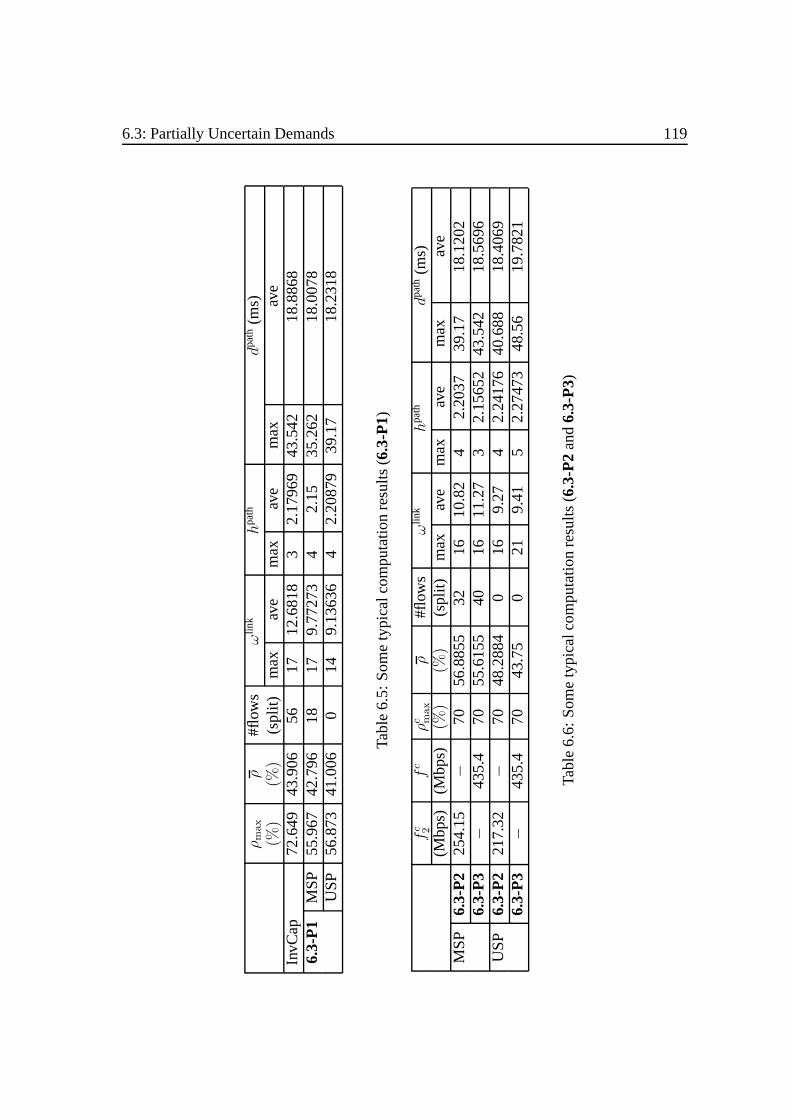
6.3: Partially Uncertain Demands 119
ρm
ax
ρ#fl
ows
ωlin
kh
path
dpa
th(m
s)(%
)(%
)(s
plit)
max
ave
max
ave
max
ave
InvC
ap72
.649
43.9
0656
1712
.681
83
2.17
969
43.5
4218
.886
86.
3-P
1M
SP
55.9
6742
.796
1817
9.77
273
42.
1535
.262
18.0
078
US
P56
.873
41.0
060
149.
1363
64
2.20
879
39.1
718
.231
8
Tabl
e6.
5:S
ome
typi
calc
ompu
tatio
nre
sults
(6.
3-P
1)
fc 2
fc
ρc m
ax
ρ#fl
ows
ωlin
kh
path
dpa
th(m
s)(M
bps)
(Mbp
s)(%
)(%
)(s
plit)
max
ave
max
ave
max
ave
MS
P6.
3-P
225
4.15
−70
56.8
855
3216
10.8
24
2.20
3739
.17
18.1
202
6.3-
P3
−43
5.4
7055
.615
540
1611
.27
32.
1565
243
.542
18.5
696
US
P6.
3-P
221
7.32
−70
48.2
884
016
9.27
42.
2417
640
.688
18.4
069
6.3-
P3
−43
5.4
7043
.75
021
9.41
52.
2747
348
.56
19.7
821
Tabl
e6.
6:S
ome
typi
calc
ompu
tatio
nre
sults
(6.
3-P
2and
6.3-
P3)

120 Chapter 6: Routing Optimization under Demand Uncertainty
the half of the valuef c of 435 Mbps for both cases.
Chapter 7
Summary and Outlook
The need for a robust and flexible routing control and management in IP networks isbecoming an urgent issue, in particular as the network gets complicated in terms of typeand number of applications, communication endpoints and QoS requirements. In thisdissertation, we have presented various efficient approaches for offline routing controland management in diverse IP networks, covering the classical IP networks running anIGP as well as MPLS and DS-MPLS networks.
In classical IP networks traffic is routed following the shortest paths according to the met-ric used by the IGP. Thus, routing control is not very flexible in this respect, since wecan not search for better paths directly, but we have to search for abetterweight system,instead. In the literature, this problem is proven as NP complete. Our contributions in thisresearch area include: (i) proposing several algorithms to deal with metric-based trafficengineering problems in such classical and also transitional IP networks; and (ii) investi-gating the impact of partial demand increase on the network and developing a mechanismto decide when and how reoptimization should be performed. Our computational re-sults have shown that our algorithms can find better routing solutions compared to thosegiven by common routing configurations. This in turn will improve network efficiency.Concerning partial demand increase, it has been shown that depending on the policy pa-rameters and demand increase patterns, it is possible to perform minimal reconfigurationin order to keep network performance within an acceptable range.
Concerning traffic engineering, MPLS technology offers more flexibility than the classicalrouting protocols. Particularly, since it allows explicit routing to be easily implemented.Together with DiffServ, MPLS can be used to deploy flexible routing schemes based ondifferent classes of service. Unlike from most of related work in the literature, here weemphasize over-provisioning requirements as a means for providing QoS. We presentedsome novel mathematical formulations and heuristic frameworks for dimensioning of IPnetworks under such requirements and different routing strategies. The heuristics can
121
122 Chapter 7: Summary and Outlook
find good solutions very fast, although for our sample network, the linear programmingapproach (with limited computation time) can still achieve better solutions: it can saveup to 15% of the network cost compared to the result of the heuristics. Furthermore, fortraffic engineering purposes we also considered a hybrid routing scheme, where some ofthe routing paths can be explicitly specified and the rest is determined according to theIGP metrics. It has been demonstrated by our case study, that starting from an optimizedweight system for traffic aggregate, the over-provisioning factor for each traffic class, andthus the corresponding service quality, can be improved by establishing several explicitrouting paths (ER-LSPs).
Most classical planning and routing management approaches, which are based on agiventraffic matrix, requirepreciseforecast of traffic demands in order to achieve a predictablequality. This means that imprecision in a single element of the traffic matrix could re-sult in inefficient routing decisions and unpredictable performance forecast errors. In thisregard, we have presented several simple demand uncertainty models whose impacts onnetwork performance can intuitively be determined. Moreover, we have also proposedthe corresponding routing control approach and investigated their effects on resource oc-cupancy as well as on other network’s parameters. While all presented models are ableto capture specific traffic variations, resource efficiency for each model is different. Themore constraints are used in a model, the less variation is supported by the correspondingmodel, but the more efficient the usage of network resources will be. We have additionallyproposed the so-called partially uncertain demand model, which is particularly appropri-ate to deal with two different types of demands simultaneously: (i) the fixed part modelsdemands that have to be guaranteed or those that can precisely be determined; and (ii)the uncertain part models demands that vary over time. In our study using the simplehose uncertainty model, the partially uncertain model can achieve much better networkefficiency than that achieved by considering all traffic as uncertain.
The work presented here can be extended in two directions. Firstly, as shortly mentionedin Chapter 1, Internet Protocol is believed as the underlying platform for the Next Genera-tion Networks (NGNs). Hence, the approaches presented in this dissertation, in particularthose given in Chapter 5, can be extended to address planning and management problemsin a such network. Since the NGNs rely on optical networks, this intrinsically meansthat the planning activities shall consider two or more layers simultaneously (cf. themulti-layer architecture discussed in Chapter 2). Secondly, concerning integer linear pro-gramming approaches, custom implementations of the Branch and Cut (BC) or its variantBranch, Cut and Price (BCP), which exploits the specific structure of the problem underconsideration, can be considered as a promising alternative to the heuristic approachesand the standard CPLEX solver.
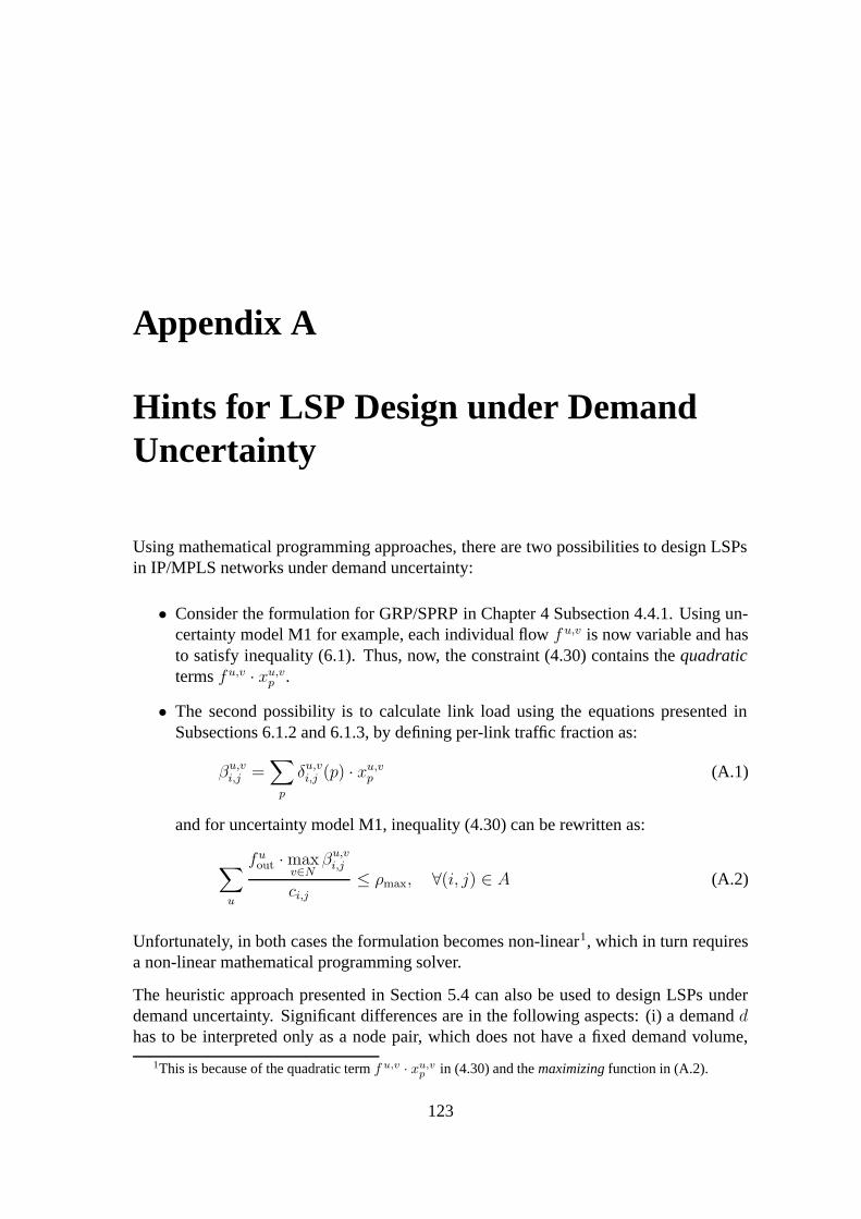
Appendix A
Hints for LSP Design under DemandUncertainty
Using mathematical programming approaches, there are two possibilities to design LSPsin IP/MPLS networks under demand uncertainty:
• Consider the formulation for GRP/SPRP in Chapter 4 Subsection 4.4.1. Using un-certainty model M1 for example, each individual flowf u,v is now variable and hasto satisfy inequality (6.1). Thus, now, the constraint (4.30) contains thequadratictermsfu,v · xu,vp .
• The second possibility is to calculate link load using the equations presented inSubsections 6.1.2 and 6.1.3, by defining per-link traffic fraction as:
βu,vi,j =∑p
δu,vi,j (p) · xu,vp (A.1)
and for uncertainty model M1, inequality (4.30) can be rewritten as:
∑u
fuout ·maxv∈N
βu,vi,j
ci,j≤ ρmax, ∀(i, j) ∈ A (A.2)
Unfortunately, in both cases the formulation becomes non-linear1, which in turn requiresa non-linear mathematical programming solver.
The heuristic approach presented in Section 5.4 can also be used to design LSPs underdemand uncertainty. Significant differences are in the following aspects: (i) a demanddhas to be interpreted only as a node pair, which does not have a fixed demand volume,
1This is because of the quadratic termf u,v · xu,vp in (4.30) and themaximizingfunction in (A.2).
123

124 Appendix A: Hints for LSP Design under Demand Uncertainty
but rather has aggregate demand behaviors as specified by traffic constraints of the corre-sponding uncertainty model; and (ii) the computation of objective functionsψ local andψ,which typically involves link load calculations, follows the equations given in Subsections6.1.2 and 6.1.3.
Finally, note that as in Chapter 4, here we considerdirectedgraphs, due to the reason thatthe ECMP rule can cause asymmetrical load distributions. However, the equations andinequalities discussed in Chapter 6 will still work for symmetrical cases. For example,using notations introduced in Chapter 5, equation (A.1) can be written follows:
βed =∑p
δedp · udp (A.3)
The formulae for computing link loads can also be rewritten analogously.

Appendix B
Acronyms
AF Assured ForwardingAR Access RouterAS Autonomous SystemATM Asynchronous Transfer ModeBA Behavior AggregateBB Branch and BoundBC Branch and CutBCP Branch, Cut and PriceBGP Border Gateway ProtocolBR Border RouterCAPEX CAPital EXpenditureCBR Constraint Based RoutingCoS Class of ServiceCR Core RouterCR-LDP Constraint-based Routing - Label Distribution ProtocolDiffServ Differentiated ServicesDSCP Differentiated Services Code PointDS-MPLS Differentiated Services - Multi-Protocol Label SwitchingECMP Equal-Cost Multi-PathEF Expedited ForwardingEGP Exterior Gateway ProtocolER-LSP Explicit Route - Label Switched PathFEC Forwarding Equivalence ClassGA Genetic AlgorithmGRP General Routing ProblemHR Hosting RouterIGP Interior Gateway Protocol
125

126 Appendix B: Acronyms
ILP Integer Linear ProgrammingIntServ Integrated ServicesIP Internet ProtocolIPM Interior Point MethodIS-IS Intermediate System to Intermediate SystemISP Internet Service ProviderIXP Internet eXchange PointLDP Label Distribution ProtocolLP Linear ProgrammingLSP Label Switched PathLSR Label Switched RouterMILP Mixed Integer Linear ProgrammingMPLS Multi-Protocol Label SwitchingMSP Multiple Shortest-PathNGN Next Generation NetworkNP Non-Polynomial deterministicNPM Network Planning and ManagementOPEX OPerational EXpenditureOP Over-ProvisioningOR Operations ResearchOSPF Open Shortest Path FirstOTN Optical Transport NetworkPHB Per-Hop BehaviorPLS Plain Local SearchPoP Point of PresencePSTN Public Switched Telephone NetworkQoS Quality of ServiceREN Research and Education NetworkRIP Routing Information ProtocolRSVP ReSource reserVation ProtocolSA Simulated AnnealingSDH Synchronous Digital HierarchySLA Service Level AgreementSPRP Single Path Routing ProblemSTM Synchronous Transport ModuleSOP Sequential Ordering ProblemTE Traffic EngineeringTCP Transport Control ProtocolToS Type of ServiceTTL Time-To-LiveUSP Unique Shortest PathWDM Wavelength Division Multiplexing
List of Figures
2.1 An example of multi-layer network architecture . . . .. . . . . . . . . . 62.2 A generic model for Network Planning and Management . . . . . . . . . 82.3 The Branch and Bound algorithm . . . . .. . . . . . . . . . . . . . . . . 112.4 An example of BB-tree . . .. . . . . . . . . . . . . . . . . . . . . . . . 112.5 An illustration of feasible regions: LP relaxation vs. convex hull . . . . . 132.6 A greedy algorithm for routing problem .. . . . . . . . . . . . . . . . . 142.7 A general Plain Local Search PLS−1 framework . . .. . . . . . . . . . 152.8 A general Plain Local Search PLS−2 framework . . .. . . . . . . . . . 152.9 An example for a variable neighborhood structure applied to PLS−2 . . . 162.10 A general Simulated Annealing framework . . . . . .. . . . . . . . . . 172.11 A general Genetic Algorithm framework .. . . . . . . . . . . . . . . . . 192.12 An example of population dynamics . . .. . . . . . . . . . . . . . . . . 192.13 A hybridization scheme between SA/GA and PLS . . .. . . . . . . . . . 212.14 Population dynamics in a hybrid GA-PLS scheme . . .. . . . . . . . . . 222.15 Hybridization of general search algorithms with simple heuristics . . . . . 23
3.1 A typical ISP architecture . .. . . . . . . . . . . . . . . . . . . . . . . . 263.2 Hop-by-hop destination-based IP routing .. . . . . . . . . . . . . . . . . 293.3 Hop-by-hop routing with ECMP . . . . .. . . . . . . . . . . . . . . . . 303.4 Routing with MPLS .. . . . . . . . . . . . . . . . . . . . . . . . . . . . 323.5 Class-based routing in a DS-MPLS network . . . . . .. . . . . . . . . . 34
4.1 Shortest path structures seen from node 1 for the case of unique and non-unique shortest path metrics. . . . . . . . . . . . . . . . . . . . . . . . 39
4.2 Block diagram for metric-based traffic engineering . .. . . . . . . . . . 404.3 A reproduction strategy . . .. . . . . . . . . . . . . . . . . . . . . . . . 434.4 Forming new Chromosomes. . . . . . . . . . . . . . . . . . . . . . . . 434.5 A simple improving heuristic for individual-based search . . . . . . . . . 444.6 The individual-based search. . . . . . . . . . . . . . . . . . . . . . . . 454.7 The topology of networknet27consisting of 27 nodes and 48 bidrectional
links . . . . . . . . . . . . . . . . . . . . . . . . . . . . . . . . . . . . . 464.8 Link utilization of networknet6before and after optimization . . . . . . . 47
127
128 List of Figures
4.9 The convergence characteristic of the HGA compared to a normal GA andthe LP lower bound foraveragepopulation fitness . . .. . . . . . . . . . 48
4.10 The convergence characteristic of the HGA compared to a normal GA andthe LP lower bound forbest individual fitness . . . . .. . . . . . . . . . 48
4.11 Result of increasing traffic for networknet27, with (4.7) as objective func-tion . . . . . . . . . . . . . . . . . . . . . . . . . . . . . . . . . . . . . 49
4.12 Result of increasing traffic for networknet27, with (4.11) as objectivefunction . . . . . . . . . . . . . . . . . . . . . . . . . . . . . . . . . . . 49
4.13 Shortest path trees for the three different scenarios : Basic IGP shortcut,IGP shortcut and Overlay .. . . . . . . . . . . . . . . . . . . . . . . . 51
4.14 Block diagram for hybrid IGP/MPLS traffic engineering . . . . . . . . . 534.15 Chromosome representation for the case of asymmetric LSPs . . . . . . . 544.16 The G-WiN network topology . . . . . .. . . . . . . . . . . . . . . . . 554.17 Source destination delays for all schemes. . . . . . . . . . . . . . . . . 574.18 The parameters measuring partial demand increase . .. . . . . . . . . . 604.19 Demand distributions before and after a partial increase withα = 10%
and an increase interval of[5, 10] Mbps . . . . . . . . . . . . . . . . . . 604.20 Increase of theρmax caused by∆F2% . . . . . . . . . . . . . . . . . . . . 604.21 Block diagram for investigation of partial demand increase . . . . . . . . 624.22 The values of∆ραmax and∆ραdiff for all α, increase-intervals and patterns
(∆Fα) . . . . . . . . . . . . . . . . . . . . . . . . . . . . . . . . . . . . 634.23 Agreenfielddimensioning approach . . .. . . . . . . . . . . . . . . . . 684.24 A capacity expansion approach . . . . .. . . . . . . . . . . . . . . . . 684.25 An example of the influence of routing for capacity expansion . . . . . . 69
5.1 Routing in an IP/MPLS network using both vanilla and ER-LSPs . . . . . 735.2 An example ISP networknet14consisting of 14 nodes and 22 bidirectional-
links . . . . . . . . . . . . . . . . . . . . . . . . . . . . . . . . . . . . . 745.3 Block diagram for joint LSP design and weight setting. . . . . . . . . . 755.4 A heuristic for installing LSPs . . . . . .. . . . . . . . . . . . . . . . . 765.5 The convergence characteristic of the hybrid SA applied to aggregate de-
mands .. . . . . . . . . . . . . . . . . . . . . . . . . . . . . . . . . . . 765.6 OP factor for both aggregate and premium traffic for the case with (b) and
without (a) ER-LSPs . . . . . . . . . . . . . . . . . . . . . . . . . . . . 775.7 Link utilization and OP factor with (b) and without (a) ER-LSPs for the
case of 3 traffic classes, applied tonet14. . . . . . . . . . . . . . . . . . . 795.8 Some illustrations showing the number of transport modules to be in-
stalled for different routing strategies and over-provisioning constraints,see text. . . . . . . . . . . . . . . . . . . . . . . . . . . . . . . . . . . . 81
5.9 Block diagram for network dimensioning tasks . . . .. . . . . . . . . . 825.10 A greedy heuristic for network dimensioning . . . . .. . . . . . . . . . 865.11 The network topologynet19used for computational studies . . . . . . . 87

List of Figures 129
5.12 Cost distribution and number of transport modules to be installed in net-work net14for the cases (i)5.2-P1, (ii) 5.2-P2and (iii) 5.2-P3 . . . . . . 89
5.13 Link utilization and OP factors for all traffic classes for5.2-P2case . . . 915.14 Routing paths in case of single-link failures . . . . . .. . . . . . . . . . 925.15 Greedy heuristic ALG−2 for network dimensioning with path protection . 965.16 Greedy heuristic ALG−3 for network dimensioning with path protection . 965.17 A greedy heuristic for multi-class network routing . . .. . . . . . . . . . 99
6.1 An example of routing demands using the ECMP rule for calculating loadupper-bounds in theoutboundmodel . . . . . . . . . . . . . . . . . . . . 106
6.2 An example of routing demands using the ECMP rule for calculating loadupper-bounds in theinboundmodel . . . . . . . . . . . . . . . . . . . . 107
6.3 Comparison of link utilization for different models using inverse capacitymetrics. . . . . . . . . . . . . . . . . . . . . . . . . . . . . . . . . . . . 109
6.4 Comparison of link utilization resulting from M1 and comparison of themaximum utilization before and after optimization . .. . . . . . . . . . 111
6.5 Comparison of the outbound, inbound and hose model. . . . . . . . . . 1146.6 Outbound (inbound) traffic from (to) each node . . . .. . . . . . . . . . 1176.7 Capacity occupied by the demands after optimization6.3-P1for the USP
case . .. . . . . . . . . . . . . . . . . . . . . . . . . . . . . . . . . . . 1176.8 Comparison of capacity occupancy for the cases partially and fully uncer-
tain demands . . . .. . . . . . . . . . . . . . . . . . . . . . . . . . . . 118

130 List of Figures

List of Tables
4.1 Some typical computation results (L = 48) . . . . . . . . . . . . . . . . 564.2 Reoptimization results forα = 10% with different values ofε1 andε2 . . 634.3 Comparison of the number of constraints and variables in Node-Link and
Link-Path formulations for GRP and SPRP . . . . . .. . . . . . . . . . 67
5.1 Some notations used in the formulation .. . . . . . . . . . . . . . . . . 845.2 The parameters used for case studies . . .. . . . . . . . . . . . . . . . . 885.3 Some computational results for networknet6 . . . . . . . . . . . . . . . 885.4 Results for networknet19 . . . . . . . . . . . . . . . . . . . . . . . . . 905.5 Additional notations necessary for mathematical formulations . . . . . . 935.6 Results for networknet19, considering backup LSPs .. . . . . . . . . . 97
6.1 Several demand uncertainty models . . .. . . . . . . . . . . . . . . . . 1046.2 The parameterΩu
1 for case study. . . . . .. . . . . . . . . . . . . . . . . 1086.3 Some typical computation results for optimization based on M1 . . . . . 1126.4 Comparison of the number of elements necessary for describing demands 1156.5 Some typical computation results (6.3-P1) . . . . . . . . . . . . . . . . . 1196.6 Some typical computation results (6.3-P2and6.3-P3) . . . . . . . . . . . 119
131

132 List of Tables

Bibliography
[AC03] David Applegate and Edith Cohen. Making Intra-Domain Routing Robustto Changing and Uncertain Traffic Demands: Understanding FundamentalTradeoffs . InProceedings of ACM SIGCOMM, pages 313–324, 2003.
[ACWX02] Daniel O. Awduche, Angela Chiu, Indra Widjaja, and Xipeng Xiao.Overview and Principles of Internet Traffic Engineering. RFC 3272, In-ternet Engineering Task Force, May 2002.
[Adl02] Hans Martin Adler. Neues im G-WiN. Presentation slides, 37. DFN Be-triebstagung, November 2002.
[AL03] Emile Aarts and Jan Karel Lenstra, editors.Local Search in CombinatorialOptimization. Princeton University Press (Reprint), New Jersey, March2003.
[ALM +01] Andreetto Alessandra, Carlo Licciardi, Corrado Moiso, David McCartney,Didier Neveux, J. C. Samou, Jorge Pinto, Jose David Mendes, Jose Mi-randa, L. Morand, Lidia Amaral, Michael Walkden, P. Fouquart, PauloChainho, Stephane Tuffin, and Sylvain Corre. Next Generation Networks:The Service Offering Standpoint. Technical Information Project P1109,EDIN 0241-1109, EURESCOM, Heidelberg Germany, November 2001.
[BAGLM00] Walid Ben-Ameur, Eric Gourdin, Bernard Liau, and Nicolas Michel. Deter-mining Administrative Weights for Efficient Operational Single-Path Rout-ing Management. InProceedings of the 1st Polish-German Teletraffic Sym-posium PGTS 2000, pages 169–176, September 2000.
[BAK01] Walid Ben-Ameur and Herve Kerivin. Routing of Uncertain Demands. InINFORMS, 2001.
[BAML +01] Walid Ben-Ameur, Nicolas Michel, Bernard Liau, Jerome Geffard, and EricGourdin. Routing Strategies for IP Networks.Telektronikk Magazine, 2(3):145–158, 2001.
133

134 Bibliography
[Bec01] Dirk Beckmann. Algorithmen zur Planung und Optimierung modernerKommunikationsnetze. PhD thesis, Technische Universität Hamburg-Harburg, Hamburg Germany, 2001.
[BG00] Sara Baase and Allen Van Gelder.Computer Algorithms: Introductionto Design and Analysis. Addison Wesley Longman, 2000. ISBN 0-201-61244-5.
[BK99] Dirk Beckmann and Ulrich Killat. Routing and Wavelength Assignmentin Optical Networks using Genetic Algorithms.European Transactions onTelecommunications, pages 537–544, 1999.
[BK02] Andreas Bley and Thorsten Koch. Integer Programming Approaches toAccess and Backbone IP Network Planning. Technical Report ZR-02-41,ZIB, Berlin Germany, 2002.
[CIS] DiffServ - The Scalable End-to-End QoS Model. White paper, Cisco Sys-tems. Online available:http://www.cisco.com.
[CPL01] ILOG CPLEX 7.1 User’s Manual. ILOG Inc., 2001.
[DDT+00] Bertrand Decocq, Elisabeth Didelet, Francois Tillerot, Roberto Clemente,Guiseppe Ferraris, Raffaele Girardi, Nuria Gomez-Rojo, Jesus F. Lobo, An-tonio Daurell-Fosalba, Teresa Almeida, and Tivadar Jakab. Planning of Op-tical Network. Technical Information Project P709, Deliverable 3 Volume1, EURESCOM, Heidelberg Germany, 2000.
[DGG+99] Nick G. Duffield,Pawan Goyal, Albert Greenberg, Partho Mishra, K. K.Ramakrishnan, and Jacobus E. van der Merive. A Flexible Model for Re-source Management in Virtual Private Networks. InProceedings of ACMSIGCOMM, Computer Communication Review, volume 29, pages 95–108,October 1999.
[DR00] Bruce Davie and Yakov Rekhter.MPLS Technology and Applications. Mor-gan Kaufmann Publishers, San Francisco, 2000. ISBN 1-55860-656-4.
[ERP02] M. Ericsson, Mauricio G. C. Resende, and Panos M. Pardalos. A GeneticAlgorithm for the Weight Setting Problem in OSPF Routing.Journal ofCombinatorial Optimization, 6:299–333, 2002.
[FE02] Clarence Filsfils and John Evans. Engineering a Multiservice IP Backboneto Support Tight SLAs.International Journal of Computer and Telecom-munications Networking, 40(1):131–148, 2002.

Bibliography 135
[FGL+00] Anja Feldmann, Albert Greenberg, Carsten Lund, Nick Reingold, and Jen-nifer Rexford. NetScope: Traffic Engineering for IP Networks.IEEE Net-work Magazine, special issue on Internet Traffic Engineering, pages 11–19,March/April 2000.
[FL03] Francois Le Faucher and Wai Sum Lai. Requirements for Support of Dif-ferentiated Services-aware MPLS Traffic Engineering. RFC 3564, InternetEngineering Task Force, July 2003.
[FT00] Bernard Fortz and Mikkel Thorup. Internet Traffic Engineering by Opti-mizing OSPF Weights. InProceedings of IEEE Infocom, pages 519–528,March 2000.
[FT02] Bernard Fortz and Mikkel Thorup. Optimizing OSPF/IS-IS Weights in aChanging World.IEEE Journal on Selected Areas in Communications, 20(4):756–767, 2002.
[FWD+02] Francois Le Faucher, Liwen Wu, Bruce Davie, Shahram Davari, PasiVaananen, Ram Krishnan, Pierrick Cheval, and Juha Heinanen. Multi-Protocol Label Switching (MPLS) Support of Differentiated Services. RFC3270, Internet Engineering Task Force, May 2002.
[GA04] Alan Gous and Arash Afrakhten. Traffic Engineering Through AutomatedOptimisation of Routing Metrics. InProceedings of 20th TERENA Net-working Conference, Rhodes, Greece, June 2004.
[Gou01] Eric Gourdin. Optimizing Internet Networks.OR/MS Today, 28(2):46–49,2001.
[GPS+00] P. Gajowniczek, Michal Pioro, A. Szentesi, J. Harmatos, and A. Juttner.Solving an OSPF Routing Problem with Simulated Allocation. InProceed-ings of the 1st Polish-German Teletraffic Symposium PGTS 2000, pages177–184, September 2000.
[Hui95] Christian Huitema.Routing in the Internet. Prentice Hall PTR, New Jersey,1995. ISBN 0-13-132192-7.
[ISC05] ISC Internet Domain Survey. Website, Internet Systems Consortium, 2005.Online available:http://www.isc.org.
[KB03] Stefan Köhler and Andreas Binzenhöfer. MPLS Traffic Engineering inOSPF Networks - A Combined Approach. InProceedings of 18th Inter-national Teletraffic Congress ITC 18, pages 21–30, Berlin Germany, Au-gust/September 2003.
136 Bibliography
[KP00] Piotr Karas and Michal Pioro. Optimisation Problems Related to the As-signment of Administrative Weights in the IP Networks’ Routing Proto-cols. InProceedings of the 1st Polish-German Teletraffic Symposium PGTS2000, pages 185–192, September 2000.
[Liu02] Xian Liu. Network Optimization with Stochastic Traffic Flows.Interna-tional Journal of Network Management, 12:225–234, 2002.
[Mar99] Richard Kipp Martin. Large Scale Linear and Integer Optimization: AUnified Approach. Kluwer Academic Publishers, 1999. ISBN 0-7923-8202-1.
[Mar03] Vladimir Marbukh. A Scenario Based Framework for Robust Network Pro-visioning. InProceedings of 18th International Teletraffic Congress ITC18, pages 691–700, Berlin Germany, August/September 2003.
[MK02a] Eueung Mulyana and Ulrich Killat. A Hybrid Genetic Algo-rithm Approach for OSPF Weight Setting Problem. InProceed-ings of the 2nd Polish-German Teletraffic Symposium PGTS 2002,pages 39–46, Gdansk Poland, September 2002. Online avail-able:http://www.tu-harburg.de/et6/papers/documents/Mulyana_Eueueng/PGTS2002-mulyana.pdf.
[MK02b] Eueung Mulyana and Ulrich Killat. An Alternative Genetic Algo-rithm to Optimize OSPF Weights. InProceedings of 15-th ITC Spe-cialist Seminar on Internet Traffic Engineering and Traffic Manage-ment, pages 186–192, Wuerzburg Germany, July 2002. Online avail-able:http://www.tu-harburg.de/et6/papers/documents/Mulyana_Eueueng/ITC-SS15-27-mulyana.pdf.
[MK03] Eueung Mulyana and Ulrich Killat. An Offline Hybrid IGP/MPLSTraffic Engineering Approach under LSP constraints. InProceed-ings of the 1st International Network Optimization Conference INOC2003, pages 416–421, Evry/Paris France, October 2003. Online avail-able:http://www.tu-harburg.de/et6/papers/documents/Mulyana_Eueueng/mulyana_inoc2003.pdf.
[MK04a] Eueung Mulyana and Ulrich Killat. Impact of Partial Demand Increaseon the Performance of IP Networks and Re-optimization Approaches.In Proceedings of the 3rd Polish-German Teletraffic Symposium PGTS2004, pages 275–284, Dresden Germany, September 2004. Online avail-able:http://www.tu-harburg.de/et6/papers/documents/Mulyana_Eueueng/increase_pap.pdf.

Bibliography 137
[MK04b] Eueung Mulyana and Ulrich Killat. Optimization of IP Net-works in Various Hybrid IGP/MPLS Routing Schemes. InPro-ceedings of the 3rd Polish-German Teletraffic Symposium PGTS 2004,pages 295–304, Dresden Germany, September 2004. Online avail-able:http://www.tu-harburg.de/et6/papers/documents/Mulyana_Eueueng/hybrid_pap.pdf.
[MK04c] Eueung Mulyana and Ulrich Killat. Optimizing IP Networks in a HybridIGP/MPLS Environment.Annals of Telecommunications, Special Issue onTraffic Engineering and Routing, 59(11):1373–1388, November/December2004.
[MK05a] Eueung Mulyana and Ulrich Killat. Load Balancing in IP Networks byOptimising Link Weights.European Transactions on Telecommunications,16(3):253–261, May/June 2005.
[MK05b] Eueung Mulyana and Ulrich Killat. Optimizing IP Networks for Un-certain Demands Using Outbound Traffic Constraints. InProceed-ings of the 2nd International Network Optimization Conference INOC2005, pages 695–671, Lisbon Portugal, March 2005. Online avail-able:http://www.tu-harburg.de/et6/papers/documents/Mulyana_Eueueng/eueung_r.pdf.
[MK05c] Eueung Mulyana and Ulrich Killat. Routing Optimization in IP/MPLSNetworks under Per-Class Over-Provisioning Constraints. InProceed-ings of the 2nd International Network Optimization Conference INOC2005, pages 551–556, Lisbon Portugal, March 2005. Online avail-able:http://www.tu-harburg.de/et6/papers/documents/Mulyana_Eueueng/mulyana_r.pdf.
[MKSB02] Jens Milbrant, Stefan Köhler, Dirk Staehle, and Les Berry. Decompositionof Large IP Networks for Routing Optimization. Technical Report 293,University of Würzburg, Würzburg Germany, 2002.
[MSK05] Eueung Mulyana, Henning Stahlke, and Ulrich Killat. Dimen-sioning of Multi-Class Over-Provisioned IP Networks. InPro-ceedings of 19th International Teletraffic Congress ITC 19, pages2137–2146, Beijing China, August/September 2005. Online avail-able:http://www.tu-harburg.de/et6/papers/documents/Mulyana_Eueueng/52-021W.pdf.
[MZK05] Eueung Mulyana, Shu Zhang, and Ulrich Killat. Internet Traf-fic Engineering for Partially Uncertain Demands. InProceedingsof 19th International Teletraffic Congress ITC 19, pages 809–818, Beijing China, August/September 2005. Online available:
138 Bibliography
http://www.tu-harburg.de/et6/papers/documents/Mulyana_Eueueng/46-163A.pdf.
[Pic03] Mario Pickavet. Multi-Layer TE in IP Networks Resilience. Presentationslides, COST 279, September 2003.
[PM04] Michal Pioro and Deepankar Medhi.Routing, Flow and Capacity Designin Communication and Computer Networks. Morgan Kaufmann Publishers(Elsevier), June 2004. ISBN 0-12-557189-5.
[PV03] G. N. Srinivasa Prasanna and Arun Vishwanath. Traffic Constraints Insteadof Traffic Matrices: Capability of a New Approach to Traffic Characteri-zation. InProceedings of 18th International Teletraffic Congress ITC 18,pages 681–690, Berlin Germany, August/September 2003.
[QPS+03] Bruno Quoitin, Cristel Pelsser, Louis Swinnen, Olivier Bonaventure, andSteve Uhlig. Interdomain Traffic Engineering with BGP.IEEE Communi-cations Magazine, pages 122–128, May 2003.
[Rie03] Anton Riedl. Optimized Routing Adaptation in IP Networks UtilizingOSPF and MPLS. InProceedings of IEEE 2003 International Conferenceon Communications (ICC), May 2003.
[Rob99] Thomas G. Robertazzi.Planning Telecommunication Networks. IEEEPress, New York, 1999. ISBN 0-7803-4702-1.
[Rob01] Jim W. Roberts. Traffic Theory and the Internet.IEEE CommunicationsMagazine, pages 94–99, 2001.
[SCK+03] Gero Schollmeier, Joachim Charzinski, Andreas Kirstädter, Christoph Re-ichert, Karl J. Schrodi, Yuri Glickman, and Chris Winkler. Improving theResilience in IP Networks. InProceedings of IEEE HPSR, Torino, Italy,june 2003.
[SJ99] P. A. Smith and B. Jamoussi. MPLS Tutorial and Operational Experiences.Presentation slides, NANOG 17 Meeting, October 1999.
[SKK00] Dirk Staehle, Stefan Köhler, and Ute Kohlhaas. Optimization of IP Routingby Link Cost Specification. Technical Report 256, University of Würzburg,Würzburg Germany, 2000.
[SS99] N. Shen and H. Smit. Calculating IGP Routes over Traffic EngineeringTunnels. Internet draft, Internet Engineering Task Force, December 1999.
[Tan03] Andrew S. Tanenbaum.Computer Networks. Prentice Hall PTR, NewJersey, fourth edition, 2003. ISBN 0-13-066102-3.

Bibliography 139
[TR02] Mikkel Thorup and Matthew Roughan. Avoiding Ties in Shortest Path FirstRouting. Technical report, AT&T Labs-Research, 2002.
[WE03] Indra Widjaja and Anwar I. Elwalid. Exploiting Parallelism to Boost Data-Path Rate in High-Speed IP/MPLS Networking. InProceedings of IEEEInfocom, 2003.
[WIK05a] Category : Internet Architecture. Website, Wikipedia, The Free Encyclo-pedia, 2005. Online available:http://www.wikipedia.org.
[WIK05b] Category : Computational Complexity Theory. Website, Wikipedia,The Free Encyclopedia, 2005. Online available:http://www.wikipedia.org.
[WR03] Kehang Wu and Douglas S. Reeves. Link Dimensioning and LSP Op-timization for MPLS Networks Supporting DiffServ EF and BE TrafficClasses. InProceedings of 18th International Teletraffic Congress ITC 18,pages 441–450, Berlin Germany, August/September 2003.
[WWZ01] Yufei Wang, Zheng Wang, and Leah Zhang. Internet Traffic Engineeringwithout Full Mesh Overlaying. InProceedings of IEEE Infocom, April2001.
[WZ01] Y. Wang and L. Zhang. A Scalable and Hybrid IP Network Traffic Engi-neering Approach. Internet draft, Internet Engineering Task Force, June2001.
[XHBN00] Xipeng Xiao, Alan Hannan, Brook Bailey, and Lionel M. Ni. Traffic Engi-neering with MPLS in the Internet.IEEE Network Magazine, pages 28–33,March 2000.
[XN99] Xipeng Xiao and Lionel M. Ni. Internet QoS: A Big Picture.IEEE Net-work, 13(2):8–18, March/April 1999.
[XTF+02] Xipeng Xiao, Thomas Telkamp, Victoria Fineberg, Cheng Chen, and Li-onel M. Ni. A Practical Approach for Providing QoS in the Internet Back-bone.IEEE Communications Magazine, 40(12):56–62, December 2002.

140 Bibliography

Curriculum Vitae
01/2002− 03/2006 Research assistant and Ph.D. student in the Department ofCommunication Networks at Hamburg University of Technol-ogy (TUHH), Germany
05/2001 Graduated as M.Sc. at University of Karlsruhe, Germany1998− 2001 Master student in Electrical Engineering at University of Karl-
sruhe07/1997− 12/1997 System engineer at PT. Multimedia Nusantara, Jakarta, In-
donesia04/1997 Graduated as Bachelor (S.T.) at Bandung Institute of Technol-
ogy (ITB), Indonesia1992− 1997 Bachelor student in Electrical Engineering at Bandung Insti-
tute of Technology1989− 1992 2nd secondary school at SMAN 3 Bandung, Indonesia1986− 1989 1st secondary school at SMPN 1 Majalaya Bandung1980− 1986 Primary school at SDN 1 Majalaya Bandung18/12/1974 Born in Majalaya Bandung
141


![KONZEPTION EINER INDOOR- ROUTING ANWENDUNG FÜR … · ANFORDERUNGEN: •RAUMGENAUIGKEIT •INDOOR UND OUTDOOR •[ONLINE UND OFFLINE] KONZEPT - Positionsbestimmung 18.02.2016 Hochschule](https://img.pdfslide.net/doc/110x75/5e044d16f5e6f714227ccb77/konzeption-einer-indoor-routing-anwendung-foer-anforderungen-araumgenauigkeit.jpg)


![Routing Protocols for Vehicular Adhoc Networks …cisjournal.org/journalofcomputing/archive/vol5no1/vol5no1_4.pdf · reactive approaches for routing [17]. Proactive approaches maintain](https://img.pdfslide.net/doc/110x75/5ac806c47f8b9a42358bf316/routing-protocols-for-vehicular-adhoc-networks-approaches-for-routing-17.jpg)