Kernel Based Methods

Colin Campbell,

Bristol University

1

In the second lecture we will:

� show that the standard QP SVM is only one

optimisation approach: we can use formulations

which lead to linear programming, nonlinear

programming semi-definite programming (SDP) for

example.

2

� show that there are further tasks beyond

classification/regression which can be handled by

kernel machines and we shall show that there are

different types of learning which can be performed

using kernel mechines.

3

� we shall comment on different learning algorithms

and strategies for model selection (finding kernel

parameters).

� we will consider different kernels including how to

combine kernels into composite kernels (data fusion).

4

2.1 Different types of optimisation: linear programming

and non-linear programming.

2.2 Other types of kernel problems beyond

classification/regression: novelty detection and its

applications

2.3 Different types of learning: passive and active

learning.

5

2.4 Training SVMs and other kernel machines.

2.5 Model Selection.

2.6 Different types of kernels and learning with composite

kernels.

6

2.1. A Linear Programming Approach to

Classification

The idea of kernel substitution isn’t just restricted to the

SVM framework, of course, and a very large range of

methods can be kernelised, including:

7

� can kernelise simple neural network learning

algorithms such as the perceptron, minover and the

adatron (so we can handle non-linearly separable

datasets). You can try the kernel adatron this

afternoon.

� kernel principal component analysis (kernel PCA) or

independent component analysis (kernel ICA).

� can devise new types of kernelised learning machines

(e.g. the Bayes Point Machine).

8

For example, rather than using quadratic programming it

is also possible to derive a kernel classifier using linear

programming (LP) instead:

min

[m∑

i=1

αi + Cm∑

i=1

ξi

]

9

subject to:

yi

m∑

j=1

αiK(xi, xj) + b

≥ 1− ξi

where αi ≥ 0 and ξi ≥ 0.

This classifier is, in my experience, slightly slower to

train than normal QP SVM but it is robust.

10

2.2. Novelty Detection (one-class classifiers).

Other tasks can be handled beyond

classification/regression ...

E.g. for many real-world problems the task is not to

classify but to detect novel or abnormal instances.

Examples: condition monitoring or medical diagnosis.

11

One approach: model the support of a data distribution.

Create a binary-valued function which is positive in those

regions of input space where the normal data

predominantly lies and negative elsewhere.

Various schemes possible: LP (here) or QP.

12

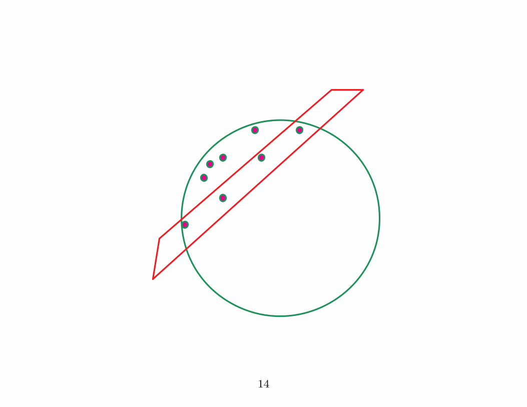
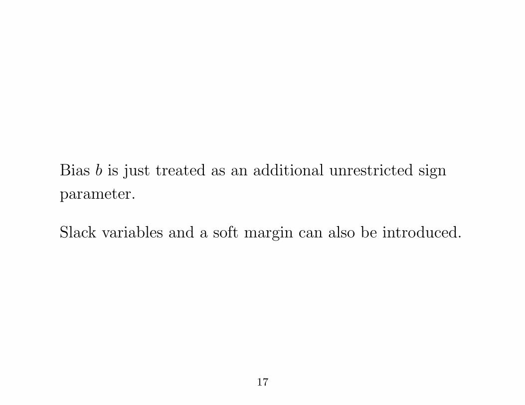
Objective: find a surface in input space which wraps

around the data clusters: anything outside this surface is

viewed as abnormal.

Feature space: corresponds to a hyperplane which is

pulled onto the mapped datapoints.

13

14

This is achieved by minimising:

W (α, b) =m∑

i=1

m∑

j=1

αjK(xi,xj) + b

15

subject to:

m∑

j=1

αjK(xi,xj) + b ≥ 0

m∑

i=1

αi = 1, αi ≥ 0

16

Bias b is just treated as an additional unrestricted sign

parameter.

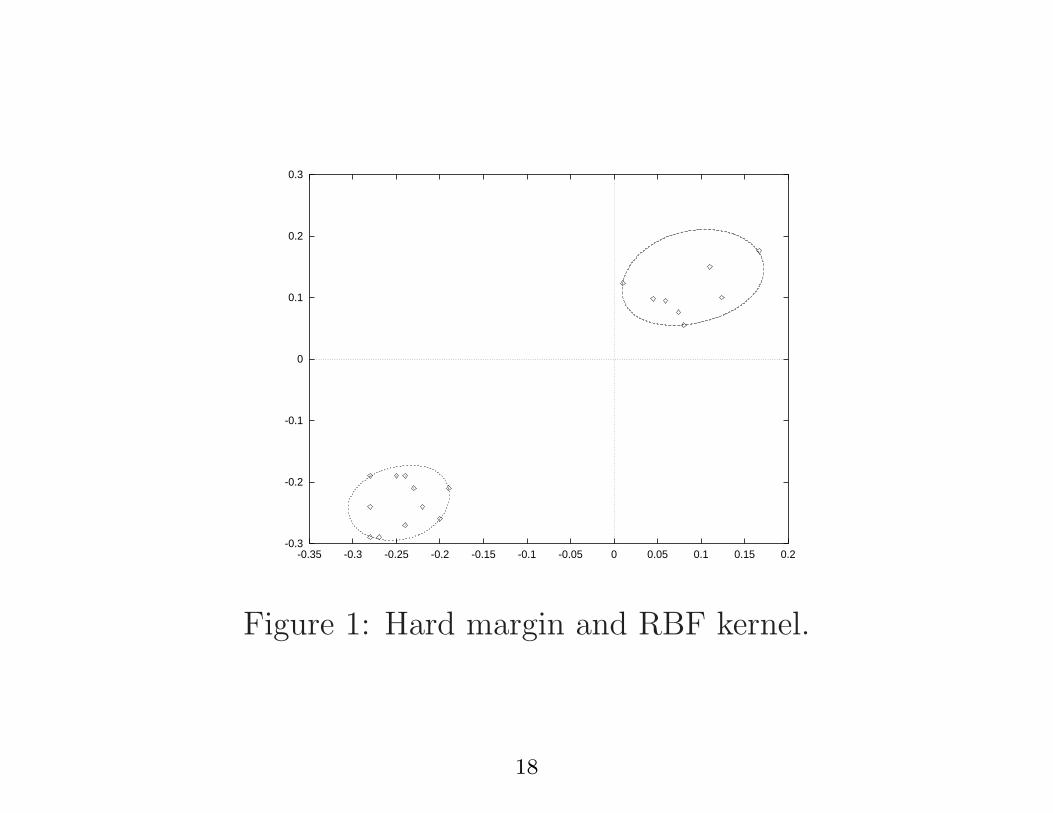
Slack variables and a soft margin can also be introduced.

17

-0.3

-0.2

-0.1

0

0.1

0.2

0.3

-0.35 -0.3 -0.25 -0.2 -0.15 -0.1 -0.05 0 0.05 0.1 0.15 0.2

Figure 1: Hard margin and RBF kernel.

18

-0.8

-0.6

-0.4

-0.2

0

0.2

0.4

0.6

0.8

-0.8 -0.6 -0.4 -0.2 0 0.2 0.4 0.6 0.8

Figure 2: Using a soft margin (with λ = 10.0)

19

-0.3

-0.25

-0.2

-0.15

-0.1

-0.05

0

0.05

0.1

0.15

0.2

-0.3 -0.25 -0.2 -0.15 -0.1 -0.05 0 0.05 0.1 0.15 0.2

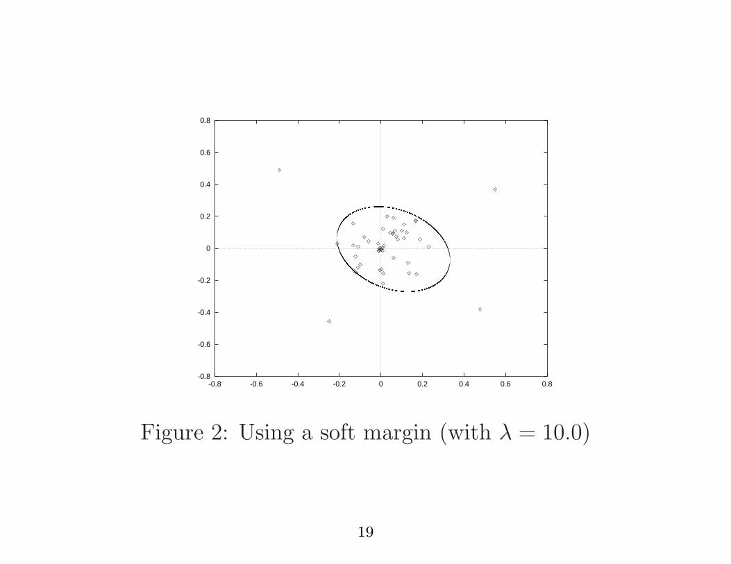
Figure 3: A modified RBF kernel

20

This basic model can be elaborated in various ways and

the choice of kernel parameter (model selection) is

important but it has worked well on real-life datasets e.g.

detecting anomalies in blood samples.

21

2.3. Different types of learning: passive vs active

learning.

Passive Learning: the learning machine receives

examples, learns these and attempts to generalize to new

instances.

Active Learning: the learning machine poses queries or

questions to the oracle or source of information (the

experimenatlist). With an efficient query learning

strategy it can learn the problem efficiently.

22

Comments on active learning:

� Several strategies are possible:

� Membership queries: the algorithm selects

unlabeled examples for the human expert to label

(e.g. handwritten character).

23

� Creating queries: can create queries and ask for

the label or answer. But sometimes the invented

examples can be meaningless and impossible to label

(e.g. I invent an unrecognisable handwritten

character).

24

Worst case: possible to invent artificial examples for

which number of queries equals sample size (hence no

advantage to query learning)

but such adverse instances don’t commonly occur in

practice.

Average case analysis has been analysed using learning

theory and we find:

25

� Active learning is better than passive learning.

� For active learning the best choice for the next query

is a point lying within the current hyperplane or as

close as possible to the current hyperplane.

26

Support Vector Machines: construct hypothesis using the

most informative patterns in the data (the support

vectors) → good candidates for active learning.

27

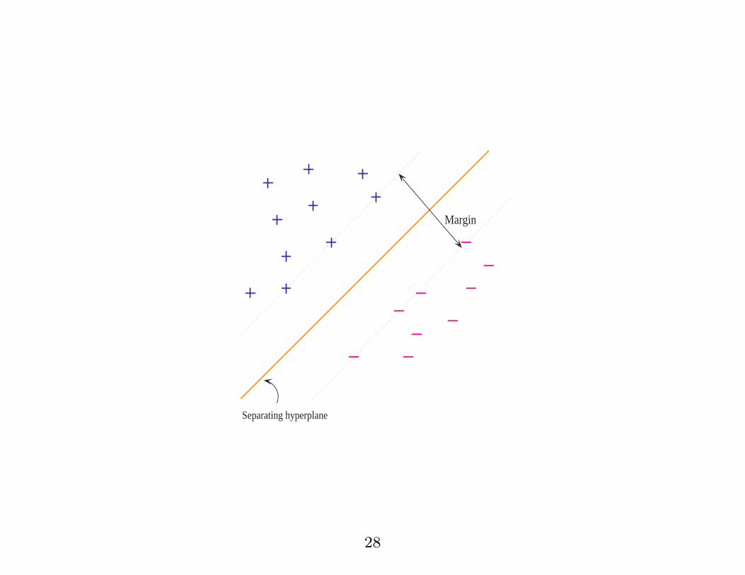
Separating hyperplane

Margin

28

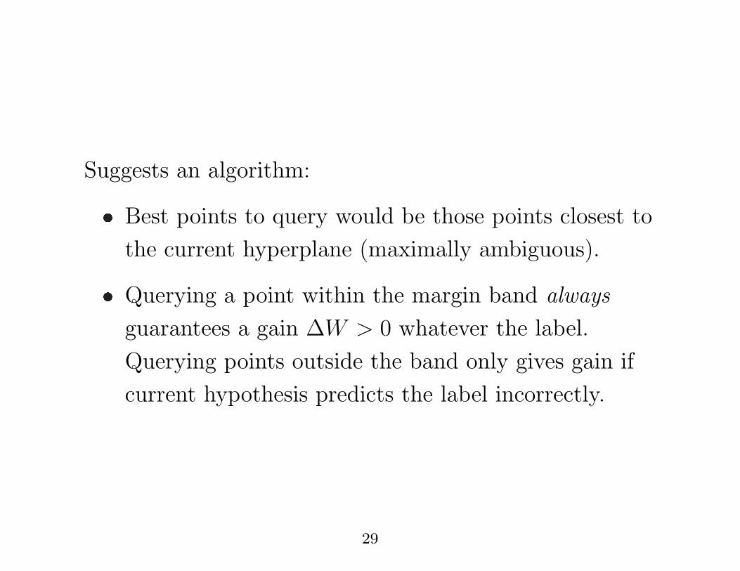
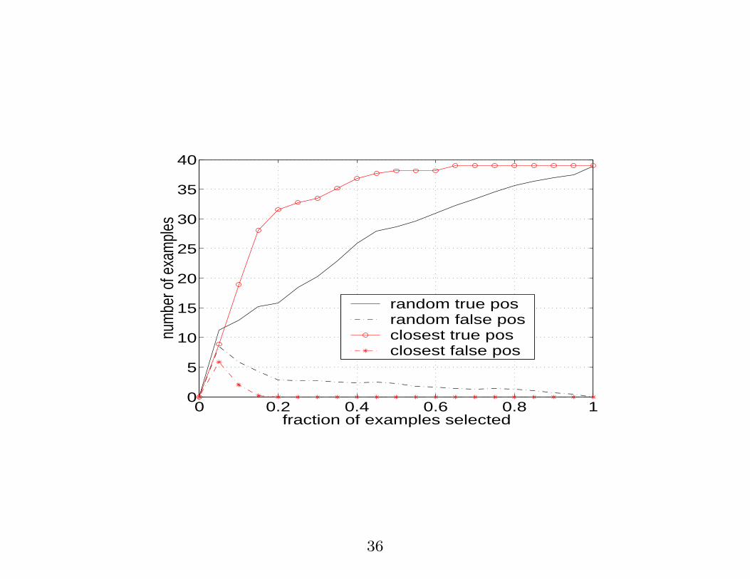
Suggests an algorithm:

� Best points to query would be those points closest to

the current hyperplane (maximally ambiguous).

� Querying a point within the margin band always

guarantees a gain ∆W > 0 whatever the label.

Querying points outside the band only gives gain if

current hypothesis predicts the label incorrectly.

29

29-1

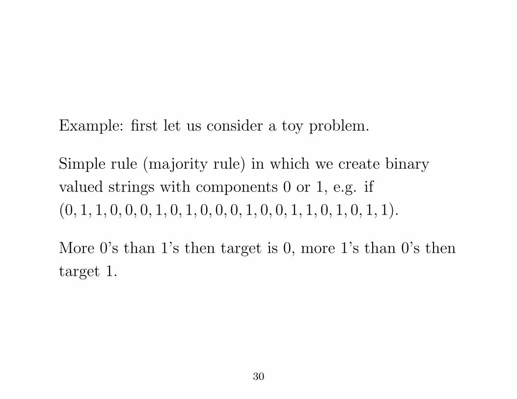
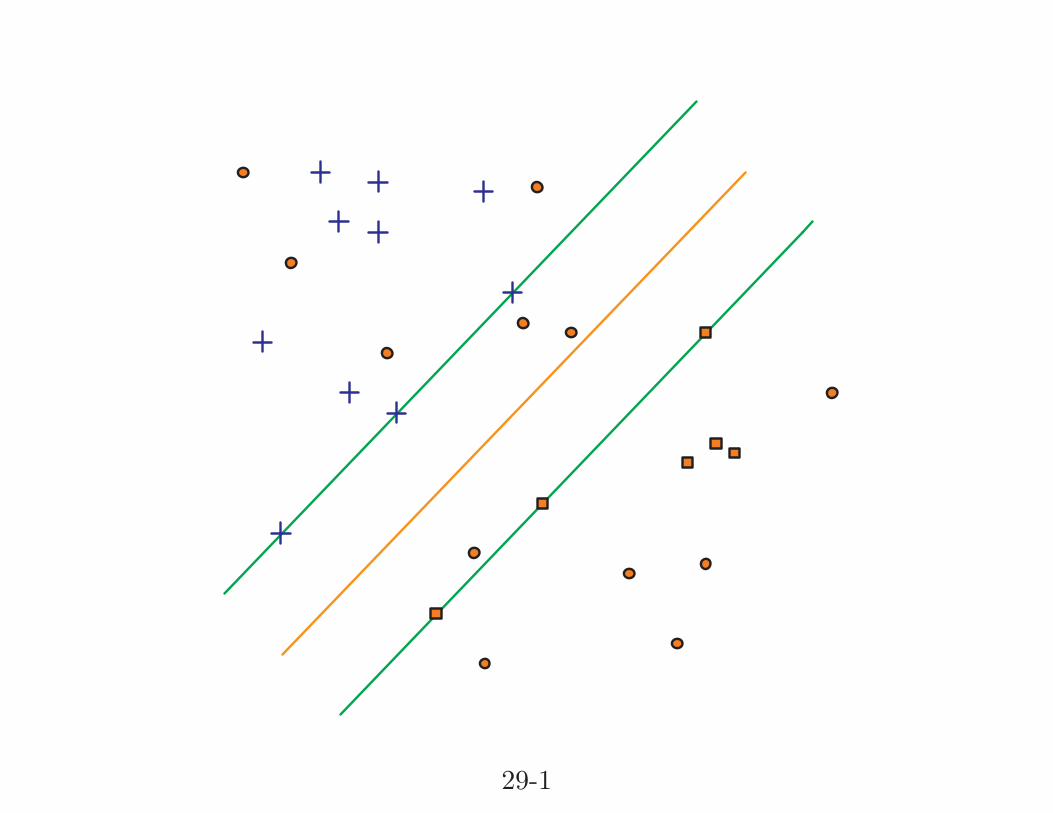
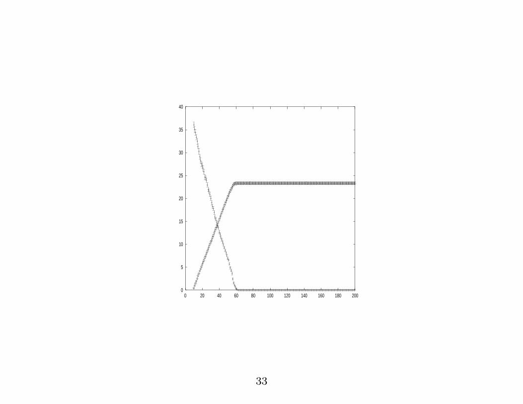
Example: first let us consider a toy problem.

Simple rule (majority rule) in which we create binary

valued strings with components 0 or 1, e.g. if

(0, 1, 1, 0, 0, 0, 1, 0, 1, 0, 0, 0, 1, 0, 0, 1, 1, 0, 1, 0, 1, 1).

More 0’s than 1’s then target is 0, more 1’s than 0’s then

target 1.

30

0

5

10

15

20

25

30

35

40

0 20 40 60 80 100 120 140 160 180 200

31

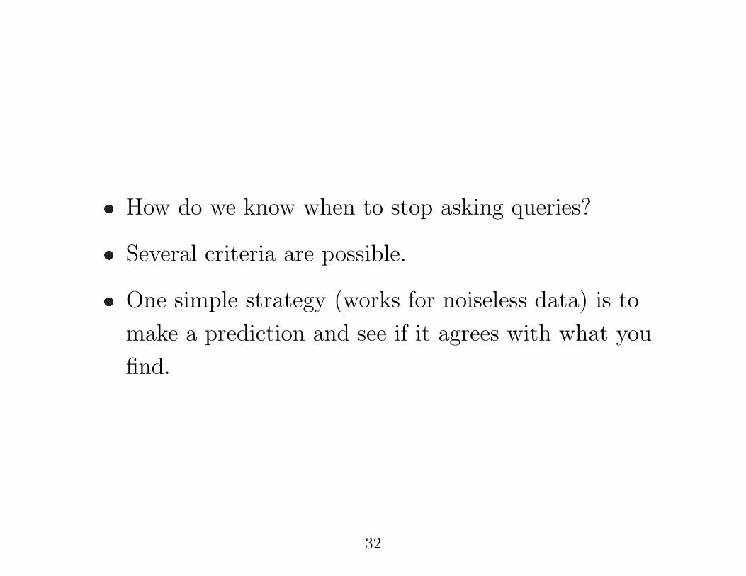
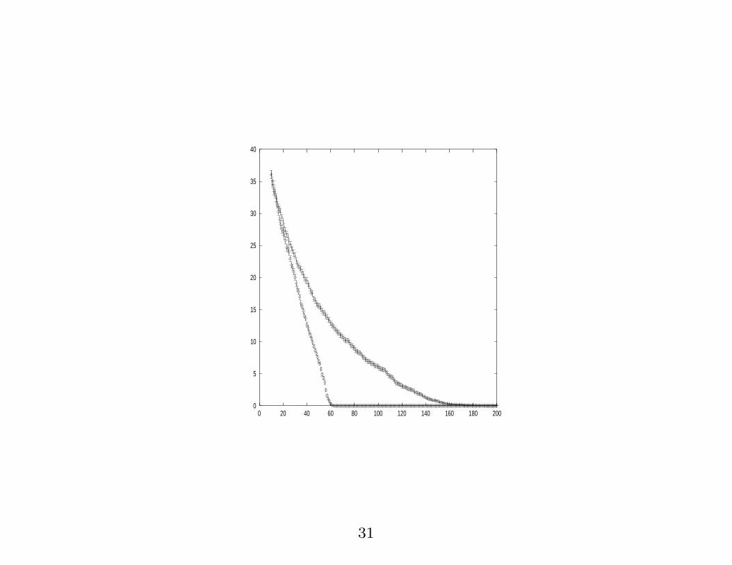
� How do we know when to stop asking queries?

� Several criteria are possible.

� One simple strategy (works for noiseless data) is to

make a prediction and see if it agrees with what you

find.

32

0

5

10

15

20

25

30

35

40

0 20 40 60 80 100 120 140 160 180 200

33

A real-life application: drug discovery

Each compound is described by a vector of 139,351

binary shape features and these vectors are typically

sparse (on average 1378 features per Round0 compound

and 7613 per Round1 compound)

34

Round0: dataset contained 1,316 chemically diverse

examples, only 39 of which are positive.

Evaluation is performed by virtual combinatorial

chemistry.

35

0 0.2 0.4 0.6 0.8 10

5

10

15

20

25

30

35

40

fraction of examples selected

num

ber o

f exa

mpl

es

random true pos random false pos closest true pos closest false pos

36

2.4. Training SVMs and other kernel machines.

So far the methods we have considered have involved

linear or quadratic programming.

Linear programming can be implemented using column

generation techniques (simplex or interior point

methods).

37

For quadratic programming e.g. conjugate gradient.

QP packages: MINOS and LOQO.

Problem: kernel matrix is stored in memory.

38

Alternatives split into three categories:

� kernel components are evaluated and discarded

during learning,

� working set methods in which an evolving subset of

data is used

� algorithms that explicitly exploit the structure of the

problem.

39

2.4.1. Chunking and Decomposition: update the αi

but using only a subset or chunk of data at each stage.

QP routine optimizes the lagrangian on an initial

arbitrary subset of data.

The support vectors found are retained and all other

datapoints (with αi = 0) discarded.

40

New working set derived from these support vectors and

additional datapoints maximally violating storage

constraints.

This chunking process iterated until margin maximized.

41

Of course, this procedure may still fail.

If so decomposition methods provide a better approach:

these algorithms only use a fixed size subset of data with

the αi for the remainder kept fixed.

42

Decomposition and Sequential Minimal

optimization (SMO).

Limiting case of decomposition in which only two αi are

optimized at each iteration.

The smallest set of parameters which can be optimized

with each iteration is plainly two if the constraint∑m

i=1

αiyi = 0 is to hold.

43

Possible to derive an analytical solution which can be

executed using few numerical operations.

Can handle classification, regression and other tasks such

as novelty detection.

44

2.4.2. Further algorithms.

Directly approach training from an optimization

perspective and create new algorithms.

Keerthi et al have proposed a very effective binary

classification algorithm based on the dual geometry of

finding the two closest points in the convex hulls.

45

The Lagrangian SVM (LSVM) method of Mangasarian

and Musicant reformulates the classification problem as

an unconstrained optimization task and then solves

problem using an algorithm requiring the solution of

systems of linear equalities.

LSVM can solve linear classification problems for millions

of points in minutes.

46

The interior-point and Semi-Smooth Support Vector

Methods of Ferris and Munson can be used to solve

linear classification problems with up to 60 million data

points in 34 dimensions.

47

2.5. Model selection and Kernel Messaging

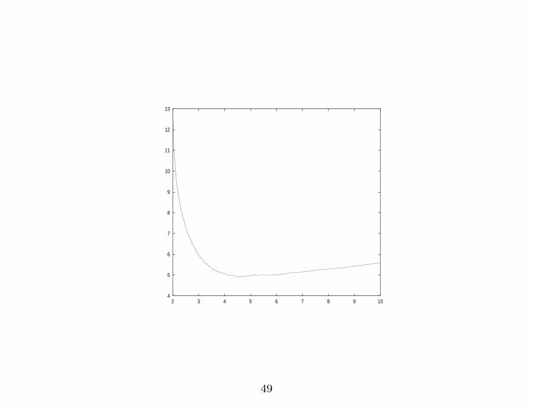
2.5.1. Model Selection. An important issue is the

choice of kernel parameter (the σ in the Gaussian kernel,

degree d of the polynomial kernel, etc).

If this parameter is poorly chosen the hypothesis

modelling the data can be oversimple or too complex

leading to poor generalisation.

48

4

5

6

7

8

9

10

11

12

13

2 3 4 5 6 7 8 9 10

49

The best value for this parameter can be found using

cross-validation of course.

However, cross-validation is wasteful of data and it would

be better to have a theoretical handle on the best choice

for this parameter.

50

A number of schemes have been proposed to indicate a

good choice for the kernel parameter without recourse to

validation data.

We will only illustrate the idea with one of these.

51

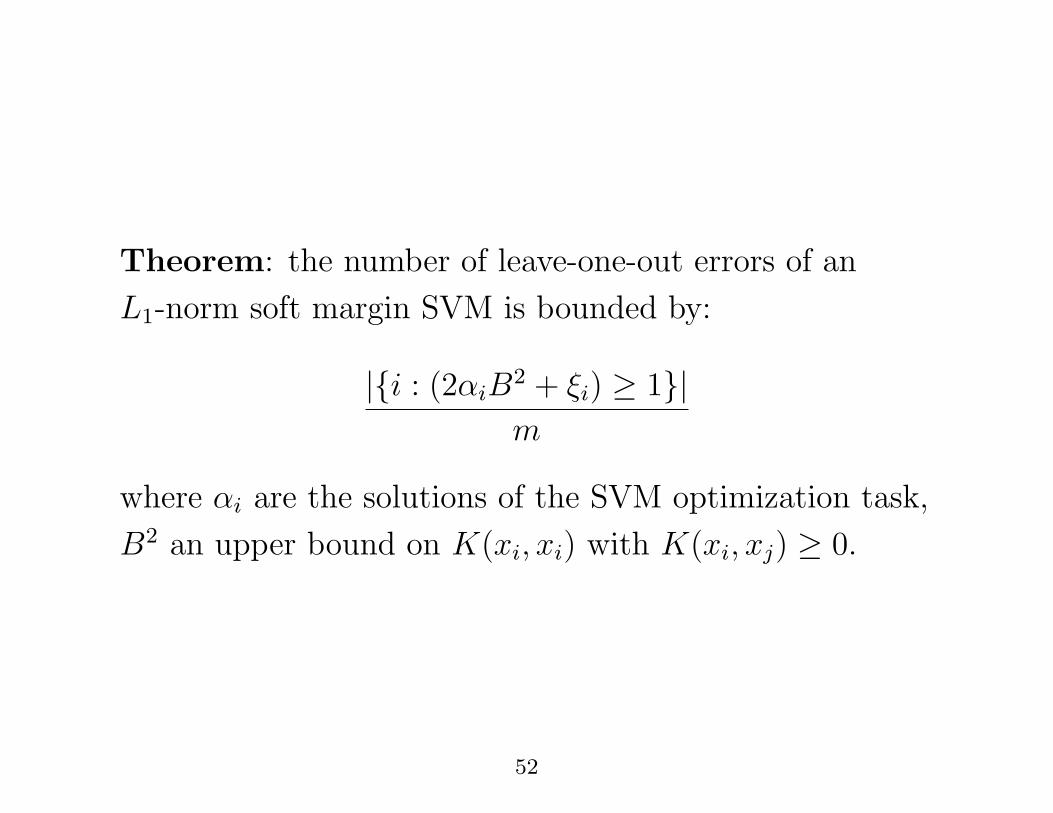
Theorem: the number of leave-one-out errors of an

L1-norm soft margin SVM is bounded by:

|{i : (2αiB2 + ξi) ≥ 1}|m

where αi are the solutions of the SVM optimization task,

B2 an upper bound on K(xi, xi) with K(xi, xj) ≥ 0.

52

Thus, for a given value of the kernel parameter, the

leave-one-out error is estimated from this quantity.

The kernel parameter is then incremented or decremented

in the direction needed to lower the LOO bound.

53

2.5.2. Kernel Massaging and Semi-Definite

Programming

Example: the existence of missing values is a common

problem in many application domains.

54

We complete the kernel matrix (compensating for missing

values) by solving the following semi-definite

programming problem:

55

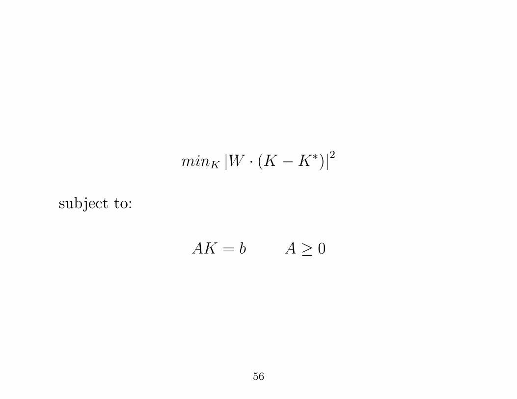
minK |W · (K −K∗)|2

subject to:

AK = b A ≥ 0

56

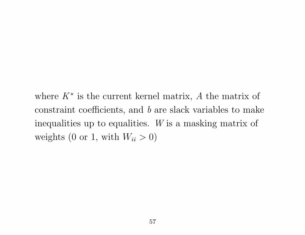
where K ∗ is the current kernel matrix, A the matrix of

constraint coefficients, and b are slack variables to make

inequalities up to equalities. W is a masking matrix of

weights (0 or 1, with Wii > 0)

57

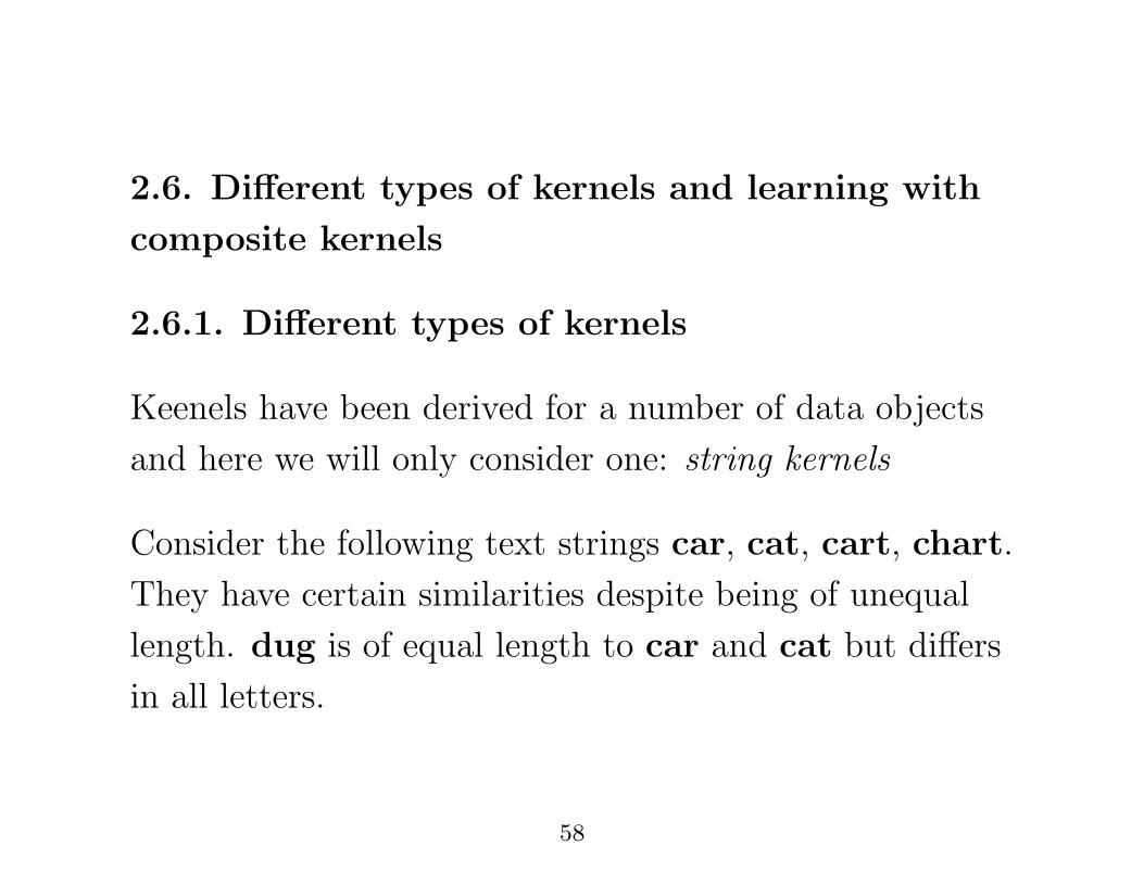
2.6. Different types of kernels and learning with

composite kernels

2.6.1. Different types of kernels

Keenels have been derived for a number of data objects

and here we will only consider one: string kernels

Consider the following text strings car, cat, cart, chart.

They have certain similarities despite being of unequal

length. dug is of equal length to car and cat but differs

in all letters.

58

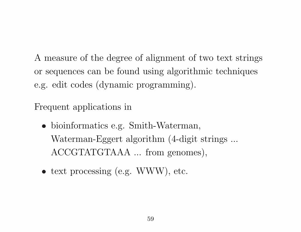
A measure of the degree of alignment of two text strings

or sequences can be found using algorithmic techniques

e.g. edit codes (dynamic programming).

Frequent applications in

� bioinformatics e.g. Smith-Waterman,

Waterman-Eggert algorithm (4-digit strings ...

ACCGTATGTAAA ... from genomes),

� text processing (e.g. WWW), etc.

59

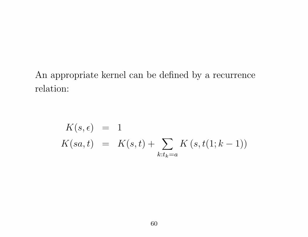
An appropriate kernel can be defined by a recurrence

relation:

K(s, ε) = 1

K(sa, t) = K(s, t) +∑

k:tk=a

K (s, t(1; k − 1))

60

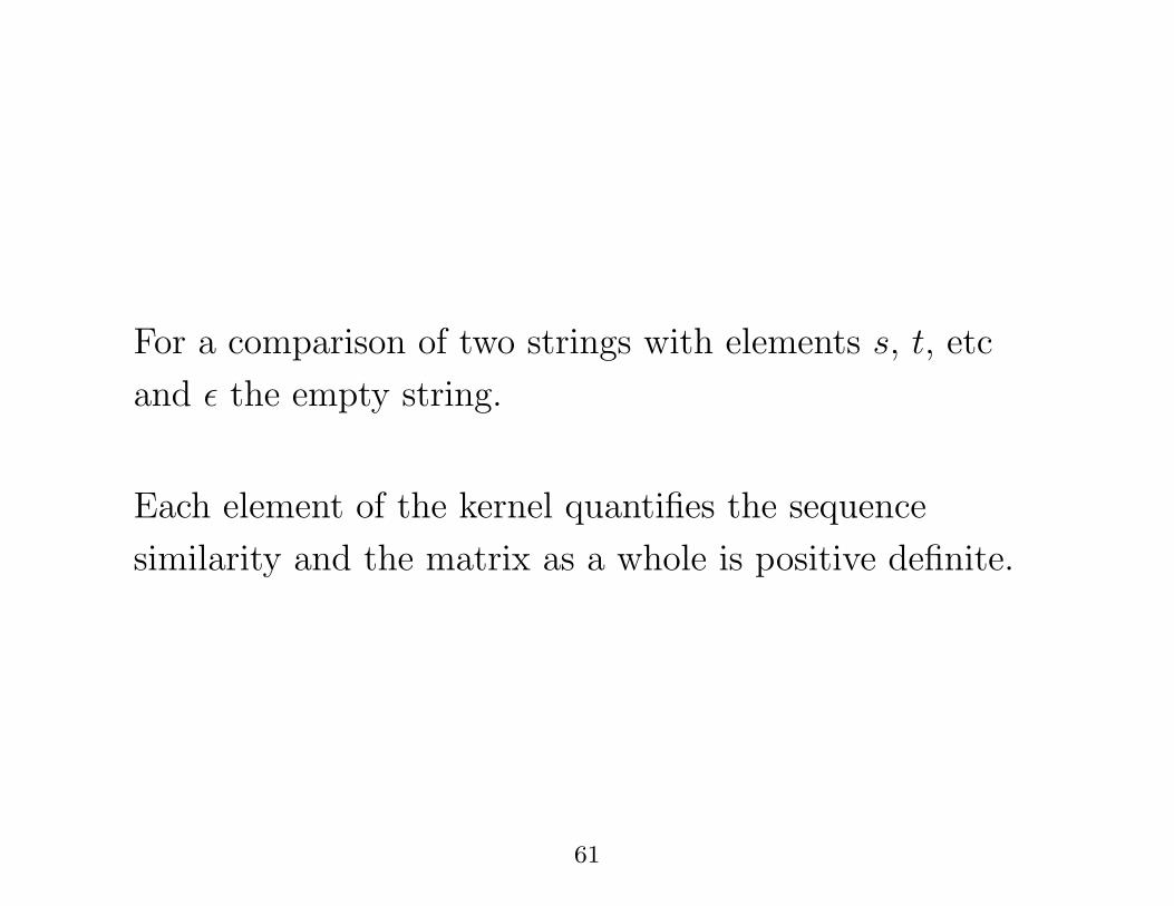
For a comparison of two strings with elements s, t, etc

and ε the empty string.

Each element of the kernel quantifies the sequence

similarity and the matrix as a whole is positive definite.

61

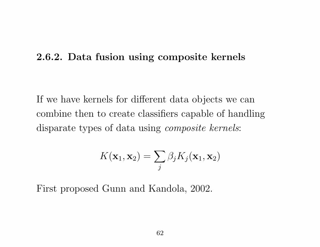
2.6.2. Data fusion using composite kernels

If we have kernels for different data objects we can

combine then to create classifiers capable of handling

disparate types of data using composite kernels:

K(x1,x2) =∑

j

βjKj(x1,x2)

First proposed Gunn and Kandola, 2002.

62

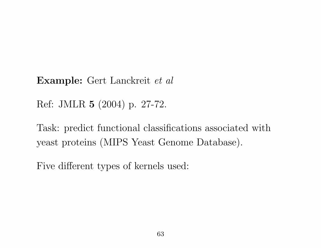
Example: Gert Lanckreit et al

Ref: JMLR 5 (2004) p. 27-72.

Task: predict functional classifications associated with

yeast proteins (MIPS Yeast Genome Database).

Five different types of kernels used:

63

� amino acid sequences (inner product kernels,

Smith-Waterman pairwise sequence comparison

algorithm kernel),

� protein-protein interactions (graph kernel, diffusion

kernel of Kondor-Lafferty),

� genetic interactions (graph kernel),

� protein complex data (weak interactions, graph

kernel),

� expression data (Gaussian kernel)

64

Find that use of all 5 kernels better than using a single

kernel.

Complex story but basically 13 functional classes:

improvement 0.71 to 0.85 for fraction correctly classified

on unseen hold-out data (0.71 is best comparator).

65

. . . but researchers are inclined to present appealing

results in their papers . . .

If one type of data is dominant (e.g. microarray versus

graph information and microarray much more plentiful)

then learning algorithm can collapse onto one kernel

(K = β1K1 + β2K2 and β2 → 0, say).

66

Despite this problem there are various successful

applications (e.g. multimedia web page classification)

and a number of proposed schemes:

� semi-definite programming (Lanckreit et al), leads to

a quadratically constrained quadratic programme

(QCQP).

� boosting schemes (Crammet et al, 2003, Bennett et

al, 2002),

� a kernelised Fisher discriminant approach (Fung et al

2004),

67

� a kernel on kernels (hyperkernels, Ong et al, 2003),

� a Bayesian strategy to find the βj coefficients for

classification and regression (Mark Girolami and

Simon Rogers, 2005, preprint, 2005), etc.

68

2.5. Applications of SVMs

Vast number number of applications: too many to

summarise here ...

Just two applications to show how useful SVMs are ...

69

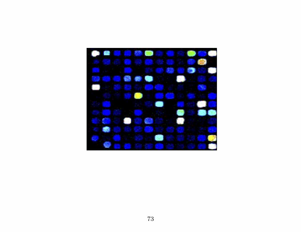
Example 1.

� Prediction of relapse/non relapse for Wilm’s tumour

using microarray technology.

� affects children/young adults

� with Richard Williams et al., ICR, London (Genes,

Chromosomes and Cancer, 2004; 41: 65-79).

70

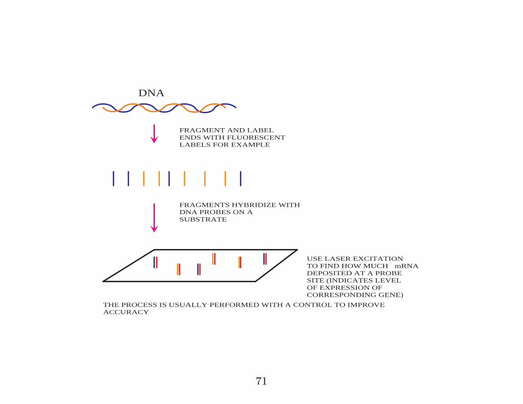
DNA

FRAGMENT AND LABEL ENDS WITH FLUORESCENT LABELS FOR EXAMPLE

FRAGMENTS HYBRIDIZE WITH DNA PROBES ON A SUBSTRATE

USE LASER EXCITATION TO FIND HOW MUCH mRNA DEPOSITED AT A PROBE SITE (INDICATES LEVEL OF EXPRESSION OF CORRESPONDING GENE)

THE PROCESS IS USUALLY PERFORMED WITH A CONTROL TO IMPROVE ACCURACY

71

72

73

� 29 examples balanced dataset with 17836 features

(probes)

� used a Support Vector Machine classifier with linear

kernel and filter method for feature scoring.

74

� impute missing values,

� log data,

� use leave-one-out testing

75

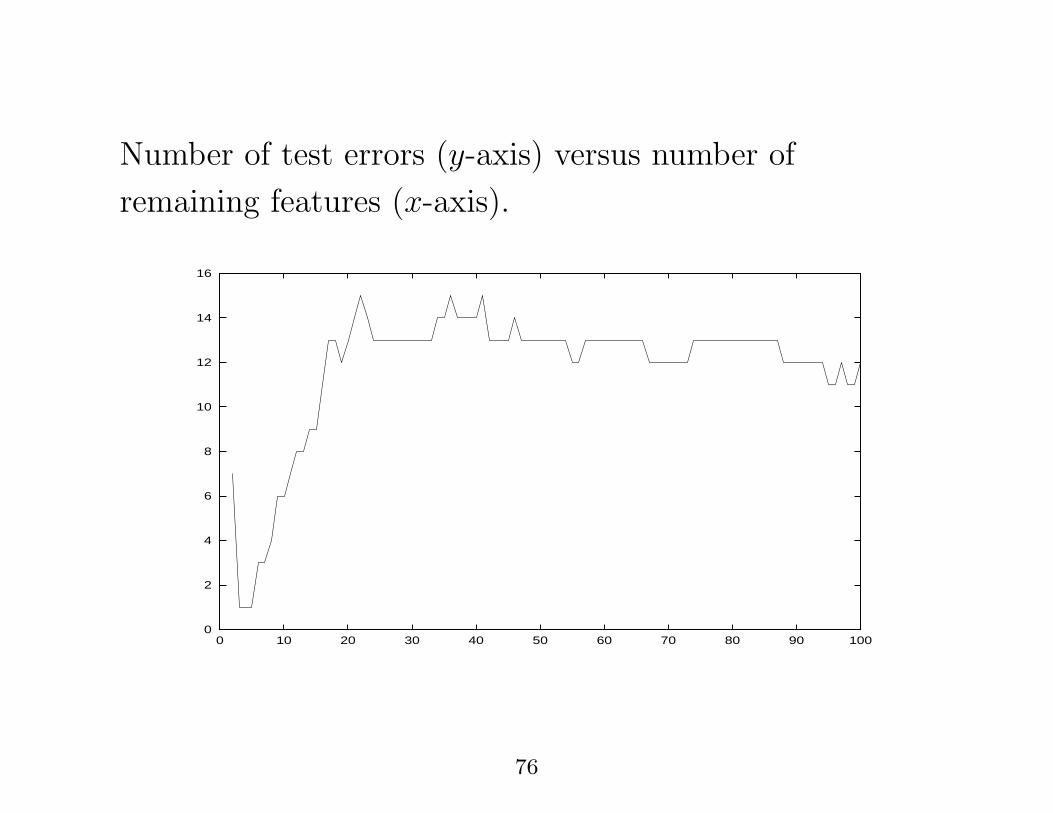
Number of test errors (y-axis) versus number of

remaining features (x-axis).

0

2

4

6

8

10

12

14

16

0 10 20 30 40 50 60 70 80 90 100

76

Example 2

Recognition of ZIP/postal codes: very important real-life

application.

Standard benchmarking dataset is NIST (60,000

handwritten characters).

AT&T (Bell Labs): state-of-the-art was a layered neural

networks (LeNet5, Yann Le Cun, et al).

77

Dennis de Coste/Bernhard Scholkopf (2002): used an

SVM but with virtual training vectors as a means of

ensuring invariant pattern recognition.

Improves on previous best by 0.15% test error reduction.

78

3. Conclusion.

Kernel methods: a powerful and systematic approach to

classification, regression, novelty detection and many

other machine learning problems.

Now widely used in many application domains including

bioinformatics, machine vision, text analysis, finance, ...

79