Embed Size (px)
Citation preview

A Bayesian Adaptive Dose Selection Procedure with
Semi-Parametric Dose-Response Modeling
Luca PozziUniversity of California, Berkeley
January 24, 2012 - 5th Annual Bayesian Biostatistics Conference, Houston, TX
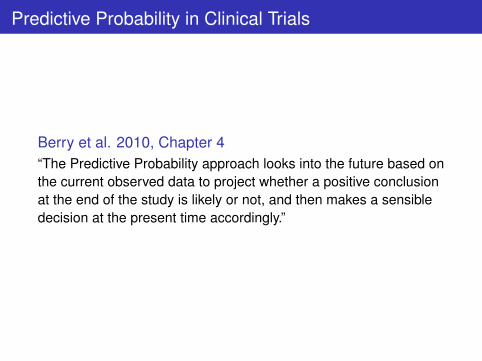
Predictive Probability in Clinical Trials
Berry et al. 2010, Chapter 4“The Predictive Probability approach looks into the future based onthe current observed data to project whether a positive conclusionat the end of the study is likely or not, and then makes a sensibledecision at the present time accordingly.”
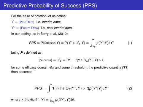
Predictive Probability of Success (PPS)
For the ease of notation let us define:
Y = {Past Data} i.e. interim data;
Y ∗ = {Future Data} i.e. post interim data.
In our setting, as in Berry et al. (2010)
PPS = P{Success|Y } = P{Y ∗ ∈ YS |Y } =
∫YS
p(Y ∗|Y)dY ∗ (1)
being YS defined as
{Success} = YS = {Y ∗ : P{θ ∈ ΘE |Y ∗,Y } > t}
for some efficacy domain ΘE and some threshold t , the predictive quantity (??)then becomes
PPS =
∫1{P{θ ∈ ΘE |Y ∗,Y } > t}p(Y ∗|Y)dY ∗ (2)
where P{θ ∈ ΘE |Y ∗,Y } =∫
ΘEp(θ|Y ∗,Y)dθ.
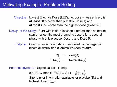
Motivating Example: Problem Setting
Objective: Lowest Effective Dose (LED), i.e. dose whose efficacy isat least 50% better than placebo (Dose 1) andat most 20% worse than the highest dose (Dose 5);
Design of the Study: Start with initial allocation 1:a:b:c:1 then at interimstop or select the most promising dose d for a secondphase with only placebo, Dose d and Dose 5;
Endpoint: Overdispersed count data Y modeled by the negativebinomial distribution (Gamma-Poisson mixture):
Y |λ ∼ Pois(λ)
λ|(α, β) ∼ Gamma(α, β)
Pharmacodynamic: Sigmoidal relationship
e.g. EMAX -model: E(D) = E0
(1 − EMAX ·D
D50%+D
).
Strong prior information available for placebo (E0) andhighest dose (EMAX );

Modeling Dose-Response Relationship
1st challenge: ModelingToo few doses to adopt Parametric Dose-Response model.(Adaptive design will start with only one lower dose)
Strategy: Semiparametric SpecificationThe mode of action of the drug and Ph.III outcomes suggest that amonotonicity constraint holds for the dose-response relationship:
Mm ={µj ≡ E[Yij] : E0 = µ1 ≥ µ2 ≥ µ3 ≥ µ4 ≥ µ5 = EMAX
}

Modeling Approach
Bayesian Model Averaging: Ingredients
1 A set of mutually exclusive modelsM = {M1, ...,MM}.To each model corresponds a probability distributionf(y |θ(m),Mm);
2 One set of priors g(θ(m)|Mm) on θ(m) for eachMm;
3 A vector of prior model probabilities π = (π1, ..., πM), πm = P{Mm},(e.g. πm = 1
M ), ∀m = 1, ...,M.
We have then:
P{success|y} =M∑
m=1
P{success|Mm, y}P{Mm |y}
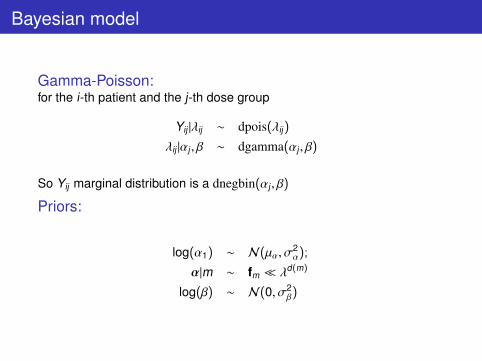
Bayesian model
Gamma-Poisson:for the i-th patient and the j-th dose group
Yij |λij ∼ dpois(λij)
λij |αj , β ∼ dgamma(αj , β)
So Yij marginal distribution is a dnegbin(αj , β)
Priors:
log(α1) ∼ N(µα, σ2α);
α|m ∼ fm � λd(m)
log(β) ∼ N(0, σ2β)
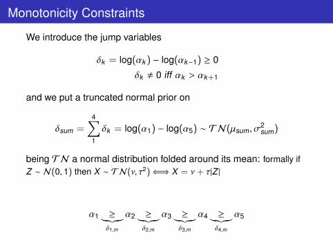
Monotonicity Constraints
We introduce the jump variables
δk = log(αk ) − log(αk−1) ≥ 0
δk , 0 iff αk > αk+1
and we put a truncated normal prior on
δsum =4∑1
δk = log(α1) − log(α5) ∼ TN(µsum, σ2sum)
being TN a normal distribution folded around its mean: formally ifZ ∼ N(0, 1) then X ∼ TN(ν, τ2)⇐⇒ X = ν + τ|Z |
α1 ≥︸︷︷︸δ1,m
α2 ≥︸︷︷︸δ2,m
α3 ≥︸︷︷︸δ3,m
α4 ≥︸︷︷︸δ4,m
α5

Jump×Model Matrix
∆ =
δ1,1 0 δ1,3 δ1,4 0 0 0 0 0 δ1,10
δ2,1 δ2,2 δ2,3 δ2,4 0 δ2,6 0 δ2,8 0 0δ3,1 δ3,2 δ3,3 0 δ3,5 δ3,6 0 0 δ3,9 0δ4,1 δ4,2 0 0 δ4,5 0 δ4,7 0 0 0
e.g. M5: µ1 = µ2 = µ3 > µ4 > µ5
α1 = α2 = α3 >︸︷︷︸δ3,5
α4 >︸︷︷︸δ4,5
α5
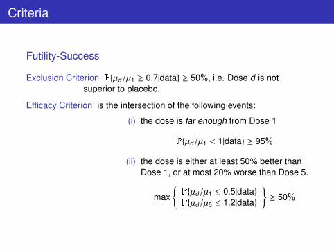
Criteria
Futility-Success
Exclusion Criterion P{µd/µ1 ≥ 0.7|data} ≥ 50%, i.e. Dose d is notsuperior to placebo.
Efficacy Criterion is the intersection of the following events:
(i) the dose is far enough from Dose 1
P{µd/µ1 < 1|data} ≥ 95%
(ii) the dose is either at least 50% better thanDose 1, or at most 20% worse than Dose 5.
max{P{µd/µ1 ≤ 0.5|data}P{µd/µ5 ≤ 1.2|data}
}≥ 50%

Interim Decision
At Interim
• if Dose 4 meets Exclusion Criterion stop for futility: no doselower than Dose 5 is effective;
• if Dose 2 meets Efficacy Criteria stop for success: Dose 2 isthe LED;
• otherwise, for each not futile Dose d calculate the PredictiveProbability of Success (PPS) and allocate to the lowestdose for which
P
{{(i)
∣∣∣Ad ,Y ,Y∗}∩
{(ii)
∣∣∣Ad ,Y ,Y∗}> 50%
∣∣∣∣Y}≥ t (3)
with Ad = {allocate to Dose d}.
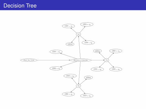
Decision Tree
Decision at Interim A3
A2
�LED = d2
A4
�LED = d4
�LED = d3
�LED = d3�LED = d2
�LED = d2
�LED = d4
�LED = d4
�LED = d3
�LED�
�LED = d5
�LED�
�LED�
Start the Trial
�LED = d2
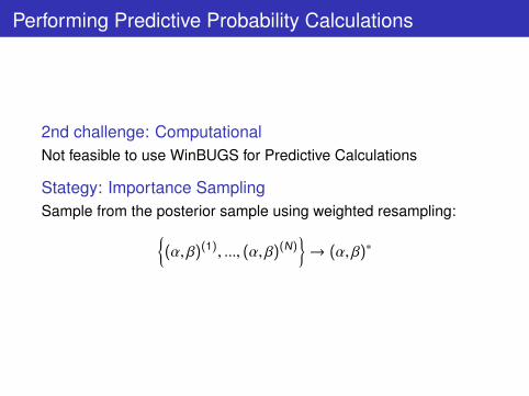
Performing Predictive Probability Calculations
2nd challenge: ComputationalNot feasible to use WinBUGS for Predictive Calculations
Stategy: Importance SamplingSample from the posterior sample using weighted resampling:{
(α, β)(1), ..., (α, β)(N)}→ (α, β)∗
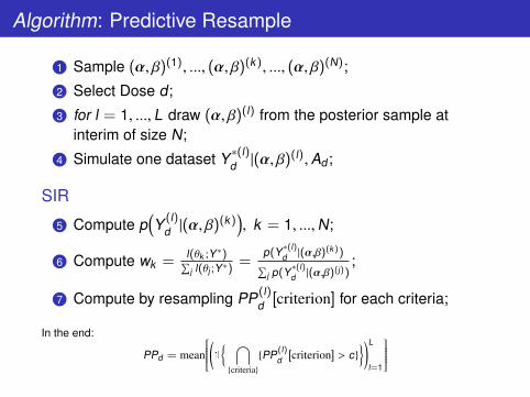
Algorithm: Predictive Resample
1 Sample (α, β)(1), ..., (α, β)(k), ..., (α, β)(N);
2 Select Dose d;
3 for l = 1, ..., L draw (α, β)(l) from the posterior sample atinterim of size N;
4 Simulate one dataset Y∗(l)d |(α, β)(l),Ad ;
SIR
5 Compute p(Y (l)
d |(α, β)(k)), k = 1, ...,N;
6 Compute wk =l(θk ;Y∗)∑j l(θj ;Y∗)
=p(Y∗(l)
d |(α,β)(k))∑j p(Y∗(l)
d |(α,β)(j));
7 Compute by resampling PP(l)d [criterion] for each criteria;
In the end:
PPd = mean
(1{ ⋂{criteria}
{PP(l)d [criterion] > c}
})L
l=1
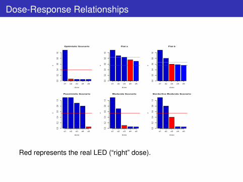
Dose-Response Relationships
Optimistic Scenario
dose
α
0.00.2
0.40.6
0.81.0
d1 d2 d3 d4 d5
Flat a
dose
α
0.00.2
0.40.6
0.81.0
d1 d2 d3 d4 d5
Flat b
dose
α
0.00.2
0.40.6
0.81.0
d1 d2 d3 d4 d5
Pessimistic Scenario
dose
α
0.00.2
0.40.6
0.81.0
d1 d2 d3 d4 d5
Moderate Scenario
dose
α
0.00.2
0.40.6
0.81.0
d1 d2 d3 d4 d5
Borderline Moderate Scenario
dose
α
0.00.2
0.40.6
0.81.0
d1 d2 d3 d4 d5
Red represents the real LED (“right” dose).

Simulation Setup
Initial Allocation: assuming we start with 1 : a : b : c : 1:• a = 0, b = 1, c = 0, i.e. 1:0:1:0:1;• a = 1, b = 1, c = 1, i.e. 1:1:1:1:1;• a = 1, b = 2, c = 1, i.e. 1:1:2:1:1.
Predictive Probability Threshold: t =
0.40.50.6
Number of Patients: split the 250 patients between the first andthe second phase:• 30% at interim and 70% for the next phase;• half at interim and half for the next phase.
Size: 500 simulations with 500 simulated studies forprediction and N = 104 for the resampling.
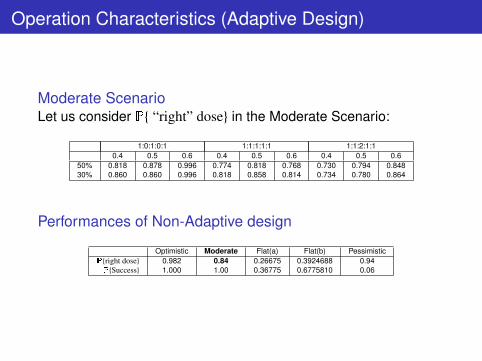
Operation Characteristics (Adaptive Design)
Moderate ScenarioLet us consider P{ “right” dose} in the Moderate Scenario:
1:0:1:0:1 1:1:1:1:1 1:1:2:1:10.4 0.5 0.6 0.4 0.5 0.6 0.4 0.5 0.6
50% 0.818 0.878 0.996 0.774 0.818 0.768 0.730 0.794 0.84830% 0.860 0.860 0.996 0.818 0.858 0.814 0.734 0.780 0.864
Performances of Non-Adaptive design
Optimistic Moderate Flat(a) Flat(b) PessimisticP{right dose} 0.982 0.84 0.26675 0.3924688 0.94P{Success} 1.000 1.00 0.36775 0.6775810 0.06

Operation Characteristics: Cheaper Solution
Expected number of patients (total sample size = 250)
1:0:1:0:1 1:1:1:1:1 1:1:2:1:150%-50% 30%-70% 50%-50% 30%-70% 50%-50% 30%-70%
Optimistic 250 250 137.75 129.67 144.5 149.67Moderate 250 250 232.25 236.67 237.75 238.67
Flat (a) 191.88 178 180.5 151.17 168.12 151.5Flat (b) 231.88 216.17 216.5 191.33 216.5 195.33
Pessimistic 250 250 183 177.33 188.67 188.33
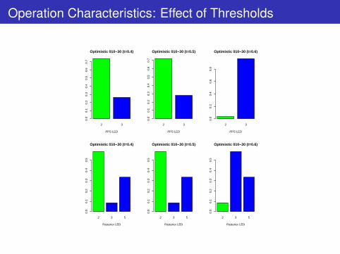
Operation Characteristics: Effect of Thresholds
2 3
Optimistic 010−30 (t=0.4)
PPS LED
0.0
0.1
0.2
0.3
0.4
0.5
0.6
0.7
2 3
Optimistic 010−30 (t=0.5)
PPS LED
0.0
0.1
0.2
0.3
0.4
0.5
0.6
0.7
2 3
Optimistic 010−30 (t=0.6)
PPS LED
0.0
0.2
0.4
0.6
0.8
2 3 5
Optimistic 010−30 (t=0.4)
Posterior LED
0.0
0.1
0.2
0.3
0.4
0.5
2 3 5
Optimistic 010−30 (t=0.5)
Posterior LED
0.0
0.1
0.2
0.3
0.4
0.5
2 3 5
Optimistic 010−30 (t=0.6)
Posterior LED
0.0
0.1
0.2
0.3
0.4
0.5

Summary
1 The procedure succeeds in detecting the properties ofdifferent Scenarios.
2 The Adaptive Design, when using an appropriate threshold, ismore efficient than the Non-Adaptive one in terms of numberof patients and not inferior in terms of sensitivity andspecificity.
3 The BMA allows for correction of suboptimal interimdecisions about the allocation.
4 Increasing the threshold we require the dose to have ahigher margin of superiority (0.6 too strict).
5 The 30%-70% proportion and the 1:0:1:0:1 allocation aredefinitely less efficient than the other configurations.

Some References
1 S. Berry, B. Carlin, J. Lee, and P. Muller, Bayesian AdaptiveMethods for Clinical Trials, CRC Press, (2010);
2 D.Ohlssen, A.Racine, A Flexible Bayesian Approach forModeling Monotonic Dose-Response Relationships in ClinicalTrials with Applications in Drug Development, ComputationalStatistics and Data Analysis,(Under Revision);
3 A.F.M Smith, A.E. Gelfand, Bayesian Statistics without Tears,The American Statistician, (1992);
4 J.A.Hoeting, D.Madigan, A.E.Raftery , C.T.Volinsky, BayesianModel Averaging: a Tutorial (with Discussion). StatisticalScience, (1999);
Acknowledgements
Thank You for Your Attention!!!
Joint work with:Heinz Schmidli, Novartis AG, Statistical MethodologyMauro Gasparini, Politecnico di Torino, Department of MathematicsAmy Racine, Novartis AG, Modeling & Simulations
Special thanks to:David Ohlssen, Novartis Pharma, Statistical Methodology