Classification in

Machine Learning

Coverage• What is Machine Learning?

• Supervised Learning - Classification

• Performance Evaluation

• Nearest Neighbor

• Naïve Bayes

• Decision Tree Learning

• Support Vector Machine

Machine Learning

A computer program is said to learn from

Experience E with respect to some class of

Tasks T and Performance measure P, if the

performance at tasks in T, as measured by P,

improves with experience E.

- Tom M. Mitchell, Machine Learning

Supervised v/s Unsupervised

Every instance in any dataset used by machine

learning algorithms is represented using the

same set of features. The features may be

continuous, categorical or binary. If instances

are given with known labels (the corresponding

correct outputs) then the learning is called

supervised, in contrast to unsupervised

learning, where instances are unlabeled.

Regression v/s Classification• Regression is the supervised learning task

for modeling and predicting continuous,

numeric variables.

For example, predicting stock price,

student’s test score or temperature.• Classification is the supervised learning task

for modeling and predicting categorical

variables.

For example, predicting email spam or not,

credit approval, or student letter grades.

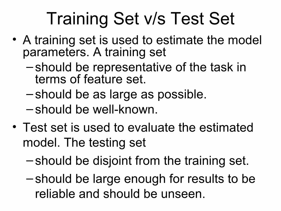
Training Set v/s Test Set• A training set is used to estimate the model

parameters. A training set– should be representative of the task in

terms of feature set.– should be as large as possible.– should be well-known.

• Test set is used to evaluate the estimated model. The testing set

– should be disjoint from the training set.

– should be large enough for results to be reliable and should be unseen.

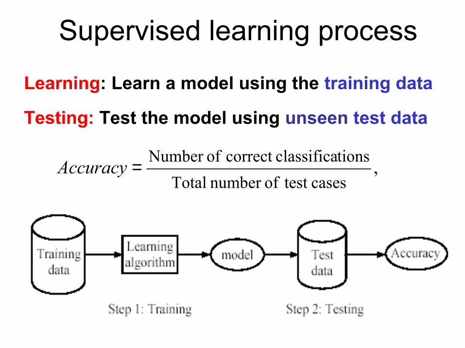
Supervised learning process

Learning: Learn a model using the training data

Testing: Test the model using unseen test data

,cases test ofnumber Total

tionsclassificacorrect ofNumber =Accuracy

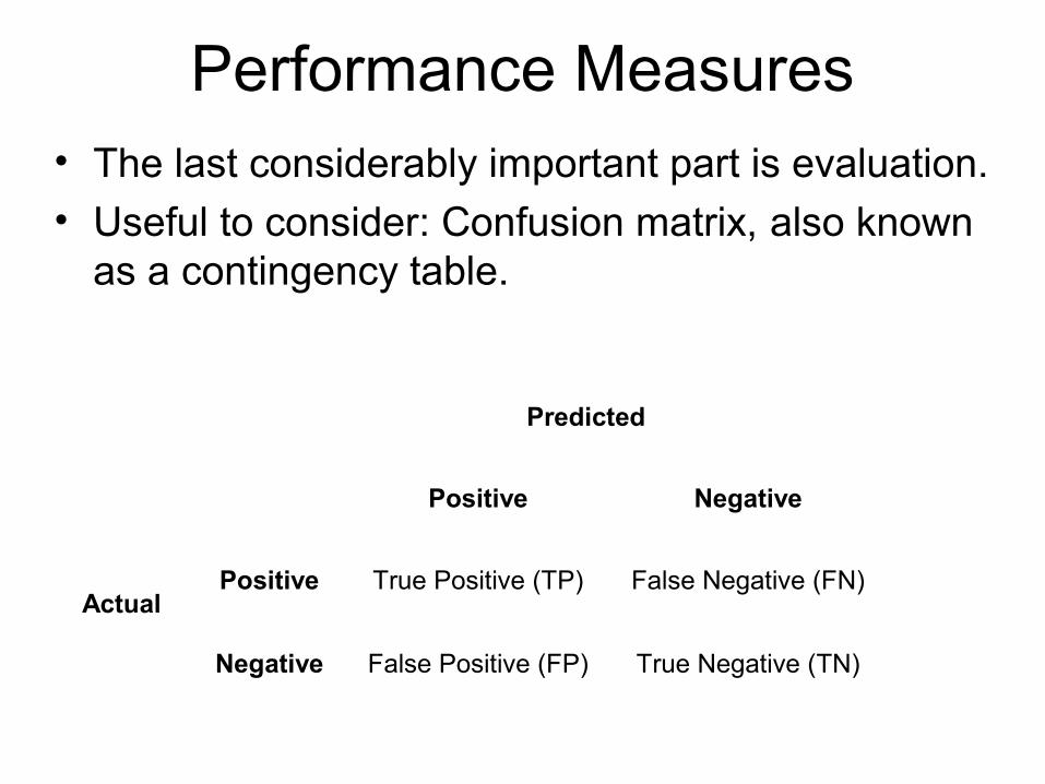
Performance Measures• The last considerably important part is evaluation.• Useful to consider: Confusion matrix, also known

as a contingency table.

Positive Negative

Positive True Positive (TP) False Negative (FN)

Negative False Positive (FP) True Negative (TN)

Predicted

Actual

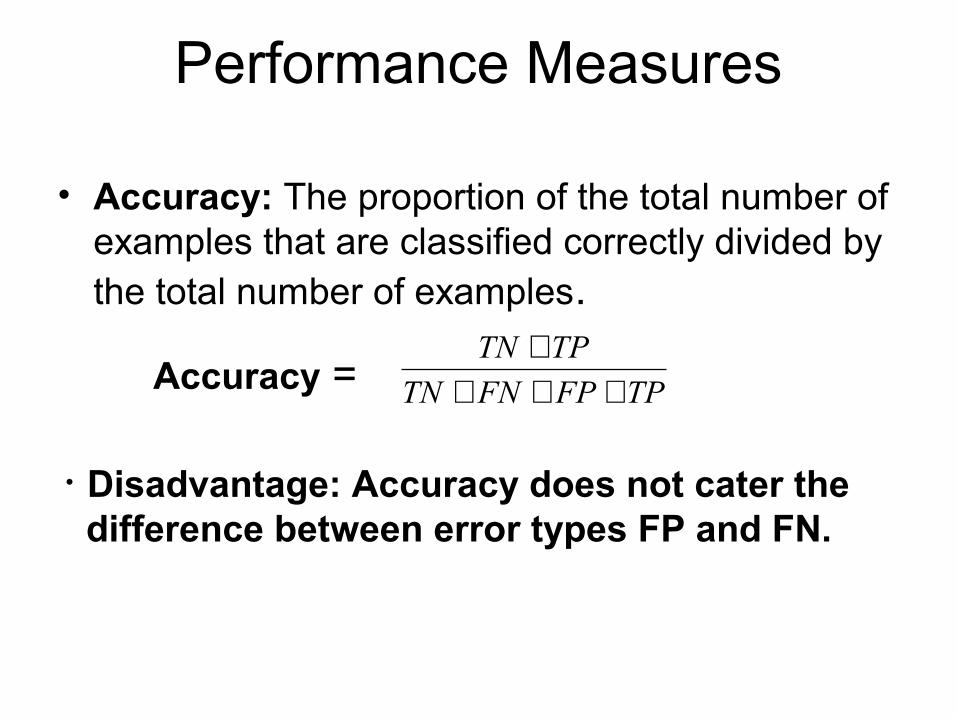
Performance Measures

• Accuracy: The proportion of the total number of examples that are classified correctly divided by the total number of examples.

Accuracy = TPFPFNTN

TPTN

++++

• Disadvantage: Accuracy does not cater the difference between error types FP and FN.

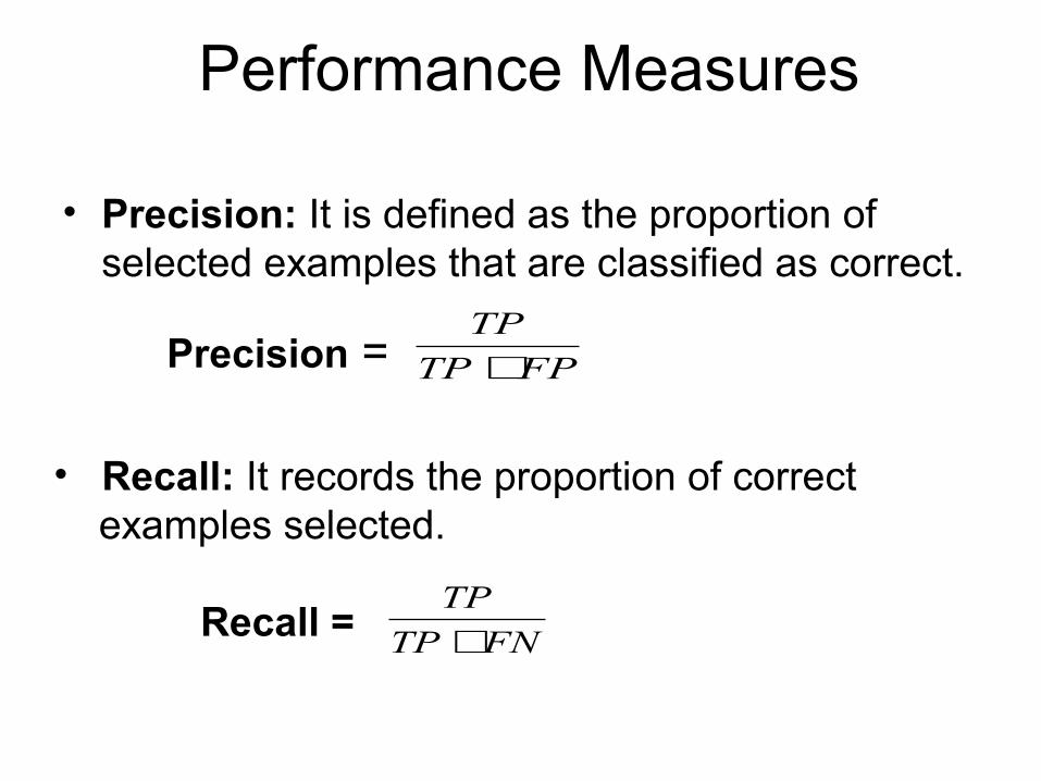
Performance Measures

• Precision: It is defined as the proportion of selected examples that are classified as correct.

Precision = FPTP

TP

+

• Recall: It records the proportion of correct examples selected.

Recall = FNTP

TP

+

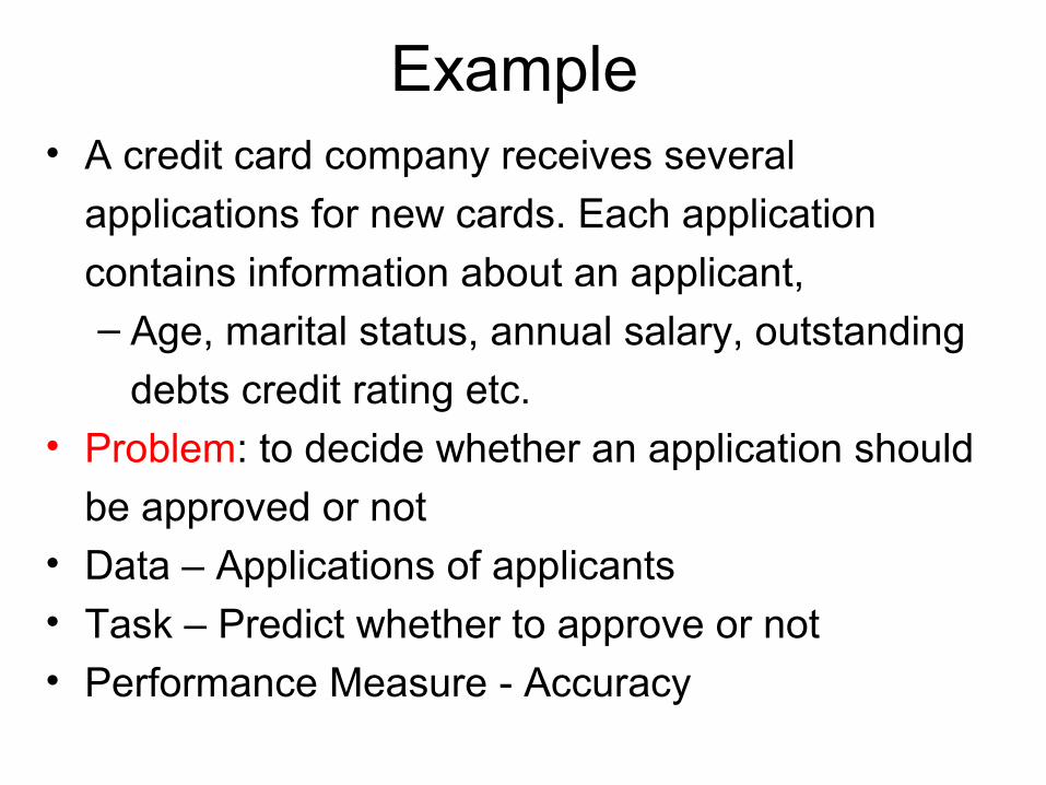
Example • A credit card company receives several

applications for new cards. Each application

contains information about an applicant, – Age, marital status, annual salary, outstanding

debts credit rating etc.• Problem: to decide whether an application should

be approved or not• Data – Applications of applicants• Task – Predict whether to approve or not• Performance Measure - Accuracy

No Free Lunch

• In machine learning, there’s something

called the “No Free Lunch” theorem. In a

nutshell, it states that no one algorithm

works best for every problem.• As a result, one should try many different

algorithms for the problem, while using

a hold-out “test set” of data to evaluate

performance and select the winner.

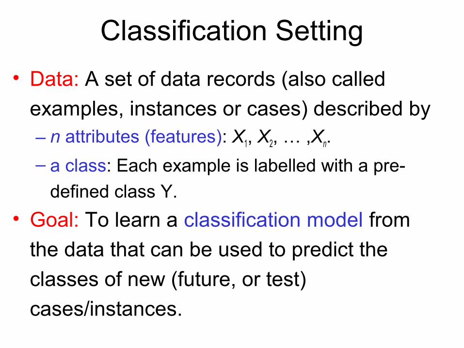
Classification Setting

• Data: A set of data records (also called

examples, instances or cases) described by– n attributes (features): X1, X2, … ,Xn.

– a class: Each example is labelled with a pre-

defined class Y.

• Goal: To learn a classification model from

the data that can be used to predict the

classes of new (future, or test)

cases/instances.

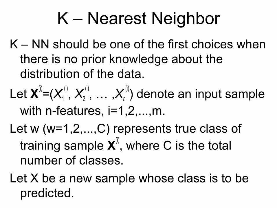
K – Nearest Neighbor

K – NN should be one of the first choices when there is no prior knowledge about the distribution of the data.

Let X(i)=(X1

(i), X2

(i), … ,Xn

(i)) denote an input sample

with n-features, i=1,2,...,m.

Let w (w=1,2,...,C) represents true class of training sample X

(i), where C is the total

number of classes.

Let X be a new sample whose class is to be predicted.

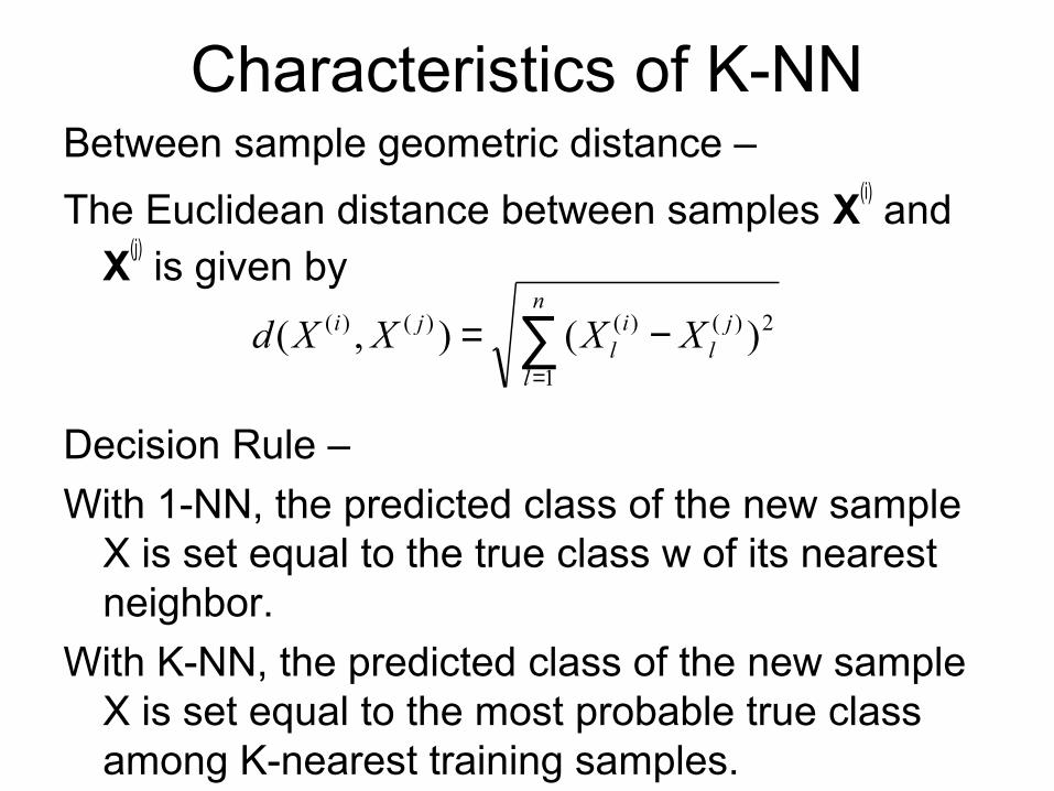
Characteristics of K-NNBetween sample geometric distance –

The Euclidean distance between samples X(i) and

X(j) is given by

Decision Rule –

With 1-NN, the predicted class of the new sample X is set equal to the true class w of its nearest neighbor.

With K-NN, the predicted class of the new sample X is set equal to the most probable true class among K-nearest training samples.

∑=

−=n

l

jl

il

ji XXXXd1

2)()()()( )(),(

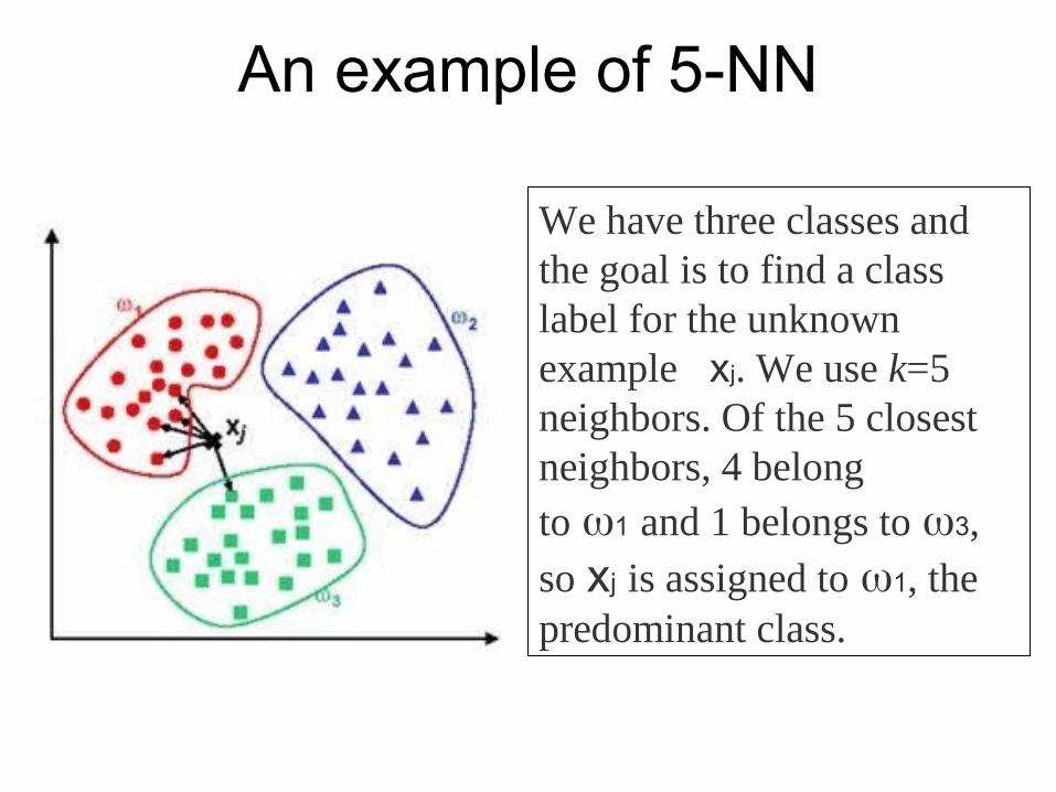
An example of 5-NN

We have three classes and the goal is to find a class label for the unknown example xj. We use k=5 neighbors. Of the 5 closest neighbors, 4 belong to ω1 and 1 belongs to ω3, so xj is assigned to ω1, the predominant class.

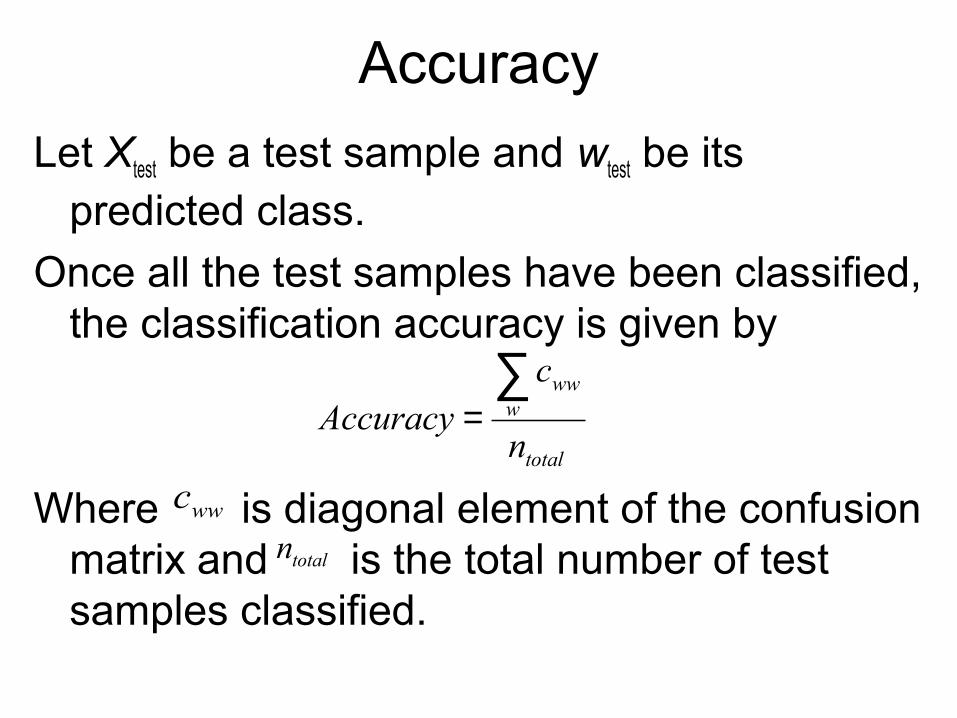
Accuracy

Let Xtest be a test sample and wtest be its predicted class.

Once all the test samples have been classified, the classification accuracy is given by

Where is diagonal element of the confusion matrix and is the total number of test samples classified.

total

www

n

cAccuracy

∑=

wwc

totaln

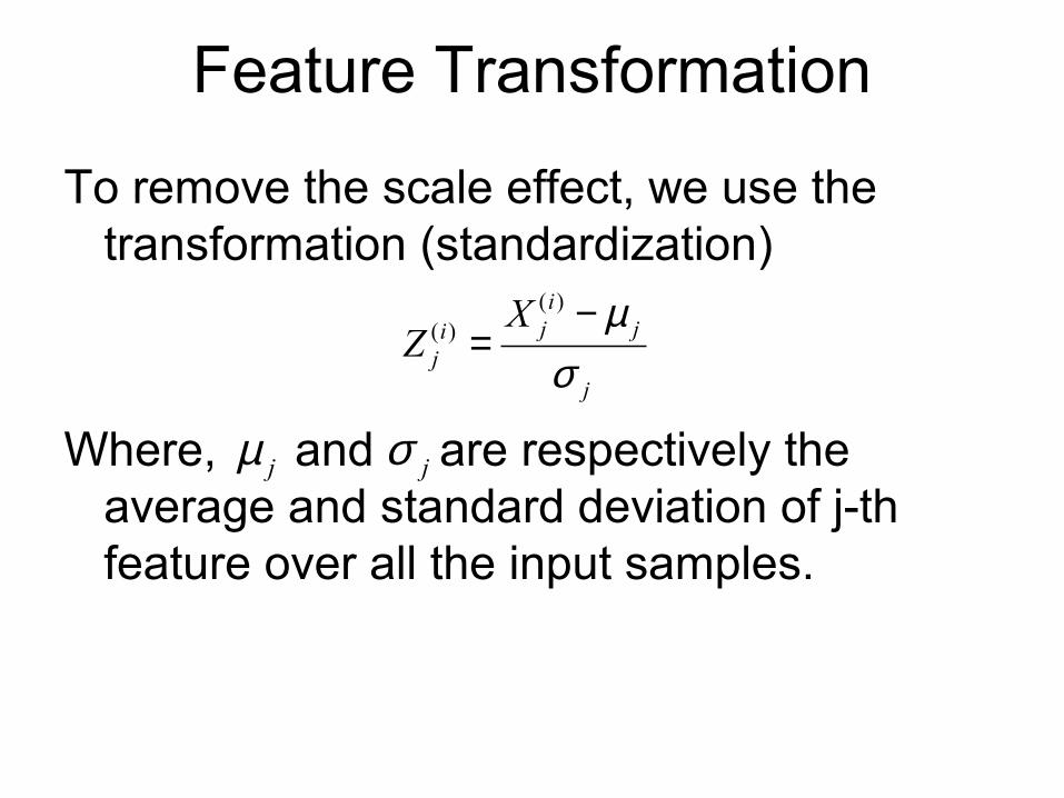
Feature Transformation

To remove the scale effect, we use the transformation (standardization)

Where, and are respectively the average and standard deviation of j-th feature over all the input samples.

j

jiji

j

XZ

σµ−

=)(

)(

jσjµ

Bayesian Learning

Importance –

Naïve Bayes classifier is one among the most practical approaches for classification.

Bayesian methods provide a useful perspective for understanding many learning algorithms.

Difficulties –

Bayesian methods require initial knowledge of many probabilities

Significant computational cost required to determine the Bayes optimal hypothesis in the general case

Bayes Theorem

Given the observed training data D, the

objective is to determine the “best”

hypothesis from some hypothesis space H.

“Best” hypothesis is considered to be the

most probable hypothesis, given the data

and any initial knowledge about the prior

probabilities of various hypotheses in the

hypothesis space H.

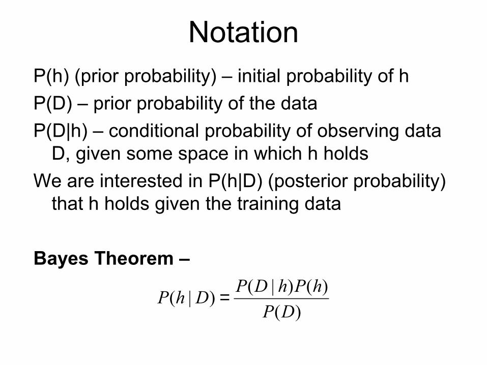
NotationP(h) (prior probability) – initial probability of h

P(D) – prior probability of the data

P(D|h) – conditional probability of observing data D, given some space in which h holds

We are interested in P(h|D) (posterior probability) that h holds given the training data

Bayes Theorem –

)(

)()|()|(

DP

hPhDPDhP =

MAP and ML

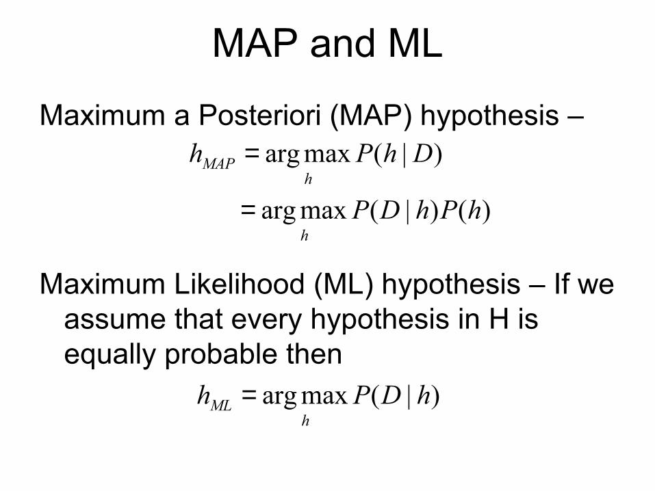
Maximum a Posteriori (MAP) hypothesis –

Maximum Likelihood (ML) hypothesis – If we assume that every hypothesis in H is equally probable then

)()|(maxarg

)|(maxarg

hPhDP

DhPh

h

hMAP

=

=

)|(maxarg hDPhh

ML =

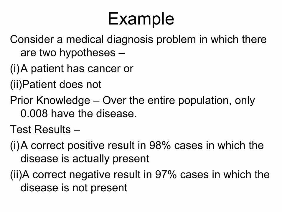
ExampleConsider a medical diagnosis problem in which there

are two hypotheses –

(i)A patient has cancer or

(ii)Patient does not

Prior Knowledge – Over the entire population, only 0.008 have the disease.

Test Results –

(i)A correct positive result in 98% cases in which the disease is actually present

(ii)A correct negative result in 97% cases in which the disease is not present

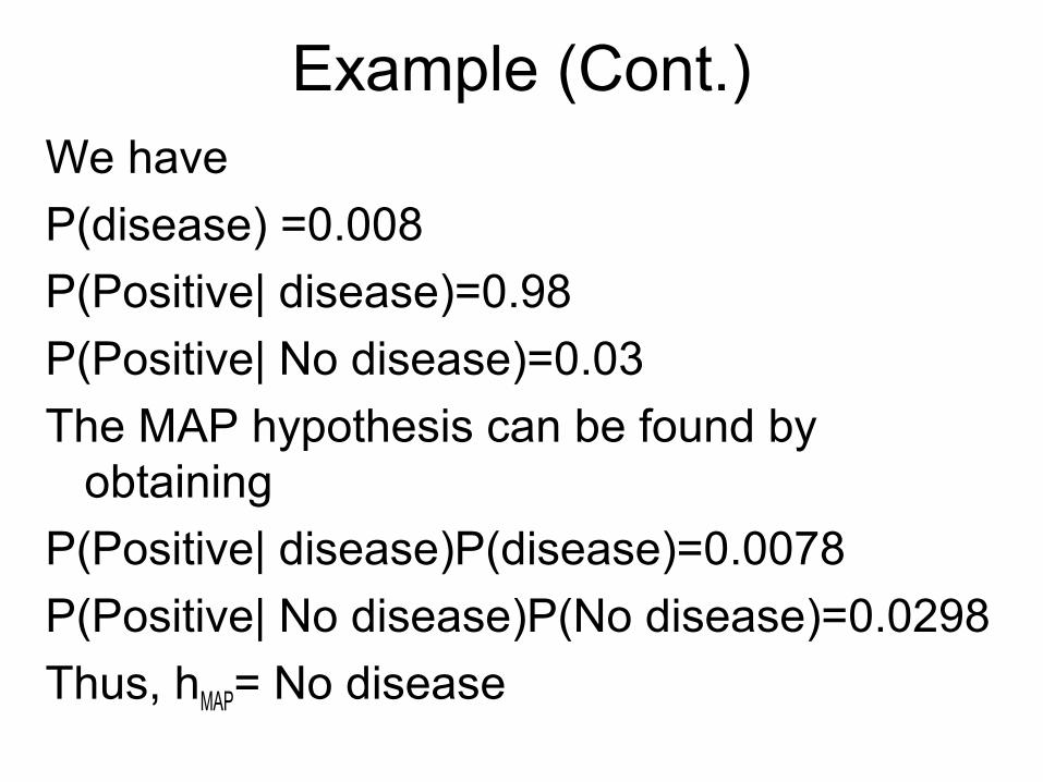
Example (Cont.)We have

P(disease) =0.008

P(Positive| disease)=0.98

P(Positive| No disease)=0.03

The MAP hypothesis can be found by obtaining

P(Positive| disease)P(disease)=0.0078

P(Positive| No disease)P(No disease)=0.0298

Thus, hMAP= No disease

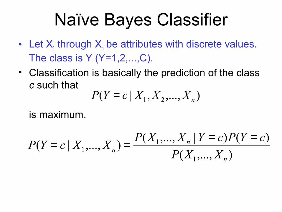
Naïve Bayes Classifier• Let X1 through Xn be attributes with discrete values.

The class is Y (Y=1,2,...,C). • Classification is basically the prediction of the class c such that

is maximum.

),...,,|( 21 nXXXcYP =

),...,(

)()|,...,(),...,|(

1

11

n

nn XXP

cYPcYXXPXXcYP

====

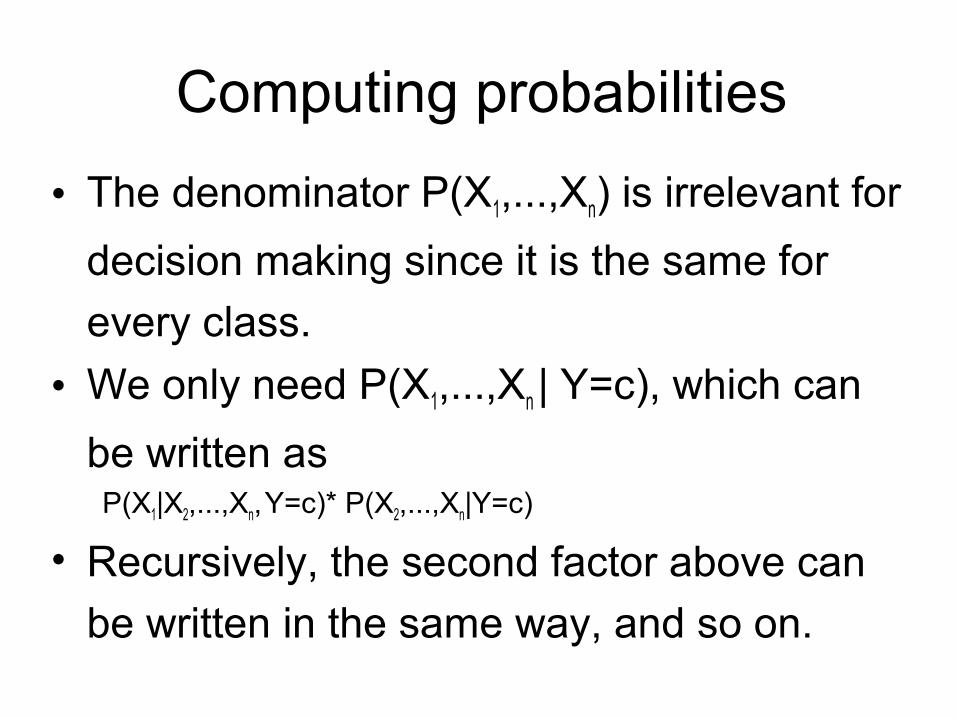
Computing probabilities

• The denominator P(X1,...,Xn) is irrelevant for

decision making since it is the same for

every class.

• We only need P(X1,...,Xn | Y=c), which can

be written as P(X1|X2,...,Xn, Y=c)* P(X2,...,Xn|Y=c)

• Recursively, the second factor above can

be written in the same way, and so on.

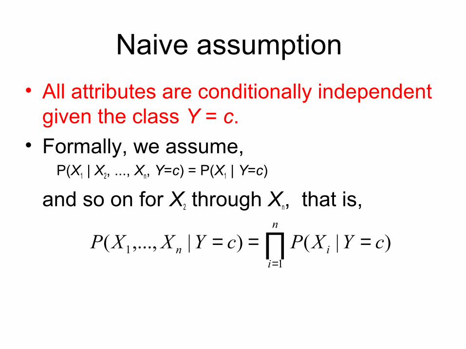
Naive assumption

• All attributes are conditionally independent given the class Y = c.

• Formally, we assume, P(X1 | X2, ..., Xn, Y=c) = P(X1 | Y=c)

and so on for X2 through Xn, that is,

∏=

===n

iin cYXPcYXXP

11 )|()|,...,(

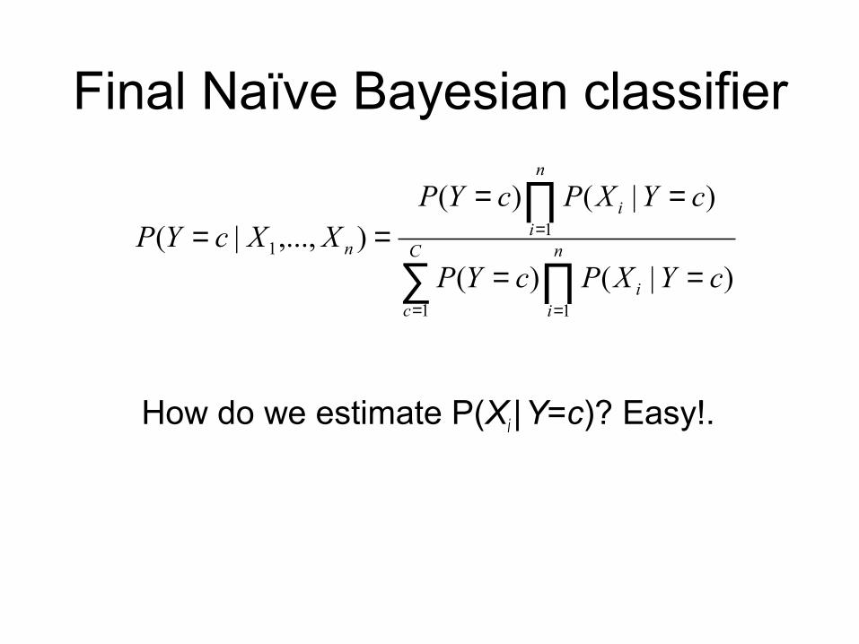
Final Naïve Bayesian classifier

How do we estimate P(Xi | Y=c)? Easy!.

∑ ∏

∏

= =

=

==

====

C

c

n

ii

n

ii

n

cYXPcYP

cYXPcYPXXcYP

1 1

11

)|()(

)|()(),...,|(

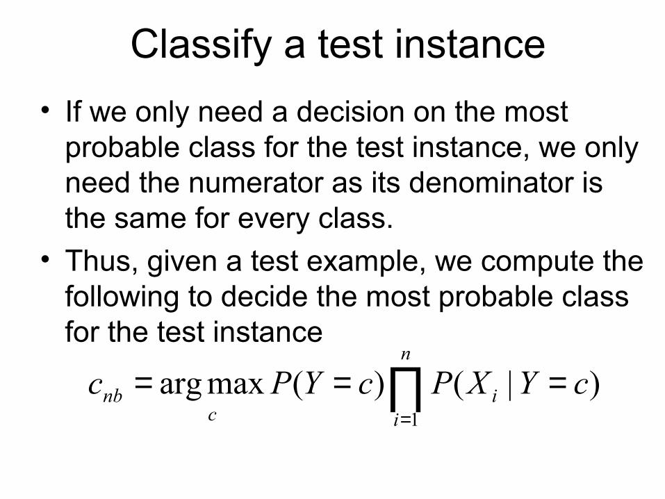
Classify a test instance

• If we only need a decision on the most probable class for the test instance, we only need the numerator as its denominator is the same for every class.

• Thus, given a test example, we compute the following to decide the most probable class for the test instance

∏=

===n

ii

cnb cYXPcYPc

1

)|()(maxarg

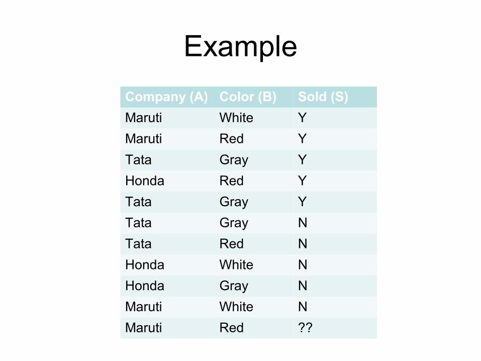
Example

Company (A) Color (B) Sold (S)

Maruti White Y

Maruti Red Y

Tata Gray Y

Honda Red Y

Tata Gray Y

Tata Gray N

Tata Red N

Honda White N

Honda Gray N

Maruti White N

Maruti Red ??

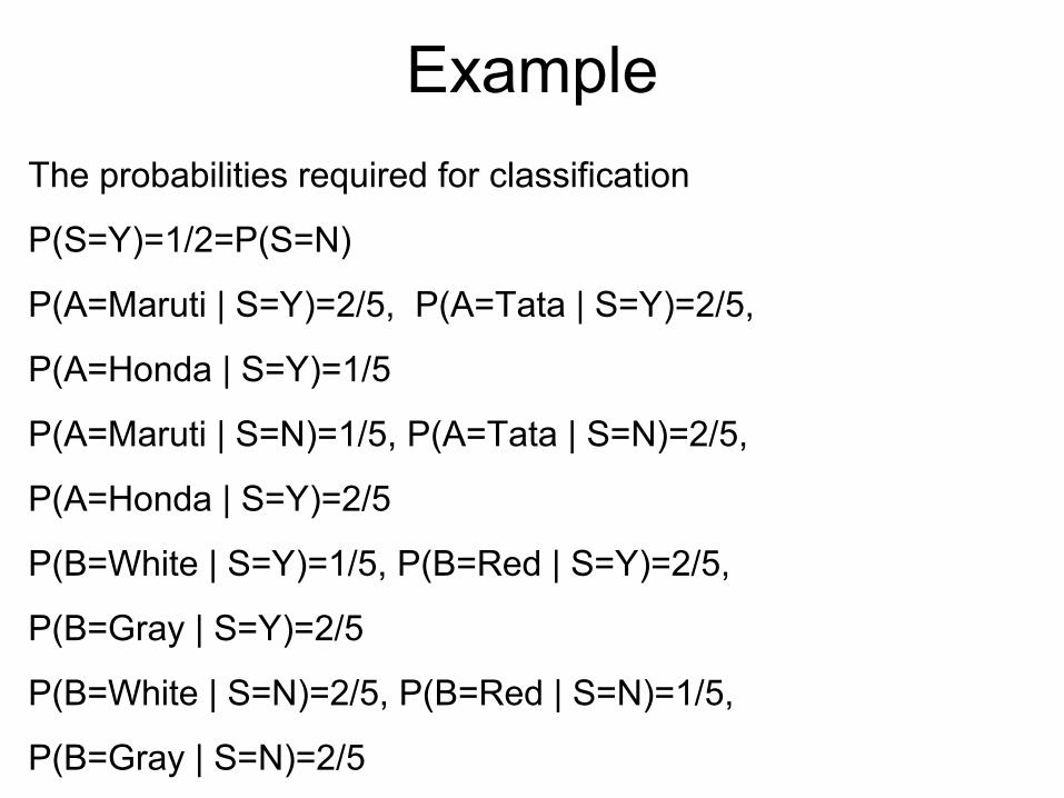
Example

The probabilities required for classification

P(S=Y)=1/2=P(S=N)

P(A=Maruti | S=Y)=2/5, P(A=Tata | S=Y)=2/5,

P(A=Honda | S=Y)=1/5

P(A=Maruti | S=N)=1/5, P(A=Tata | S=N)=2/5,

P(A=Honda | S=Y)=2/5

P(B=White | S=Y)=1/5, P(B=Red | S=Y)=2/5,

P(B=Gray | S=Y)=2/5

P(B=White | S=N)=2/5, P(B=Red | S=N)=1/5,

P(B=Gray | S=N)=2/5

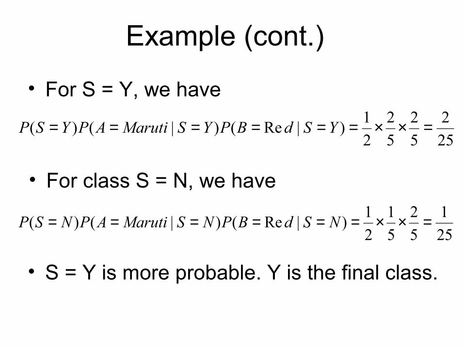
Example (cont.)

• For S = Y, we have

25

2

5

2

5

2

2

1)|Re()|()( =××====== YSdBPYSMarutiAPYSP

25

1

5

2

5

1

2

1)|Re()|()( =××====== NSdBPNSMarutiAPNSP

• S = Y is more probable. Y is the final class.

• For class S = N, we have

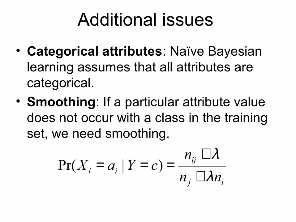
Additional issues

• Categorical attributes: Naïve Bayesian learning assumes that all attributes are categorical.

• Smoothing: If a particular attribute value does not occur with a class in the training set, we need smoothing.

ij

ijii nn

ncYaX

λλ

++

=== )|Pr(

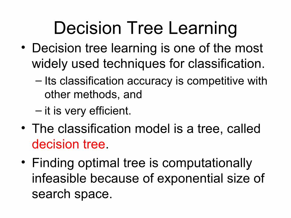
Decision Tree Learning• Decision tree learning is one of the most

widely used techniques for classification. – Its classification accuracy is competitive with

other methods, and – it is very efficient.

• The classification model is a tree, called decision tree.

• Finding optimal tree is computationally infeasible because of exponential size of search space.

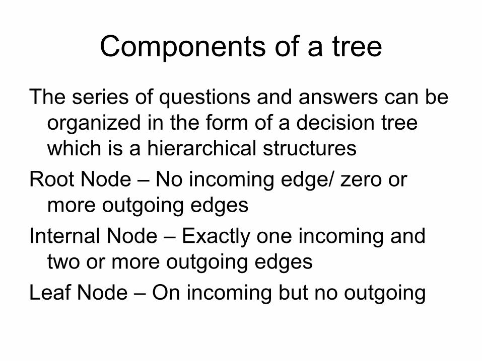
Components of a tree

The series of questions and answers can be organized in the form of a decision tree which is a hierarchical structures

Root Node – No incoming edge/ zero or more outgoing edges

Internal Node – Exactly one incoming and two or more outgoing edges

Leaf Node – On incoming but no outgoing

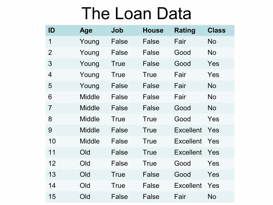
The Loan DataID Age Job House Rating Class

1 Young False False Fair No

2 Young False False Good No

3 Young True False Good Yes

4 Young True True Fair Yes

5 Young False False Fair No

6 Middle False False Fair No

7 Middle False False Good No

8 Middle True True Good Yes

9 Middle False True Excellent Yes

10 Middle False True Excellent Yes

11 Old False True Excellent Yes

12 Old False True Good Yes

13 Old True False Good Yes

14 Old True False Excellent Yes

15 Old False False Fair No

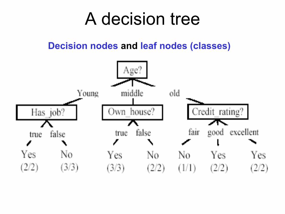
A decision treeDecision nodes and leaf nodes (classes)

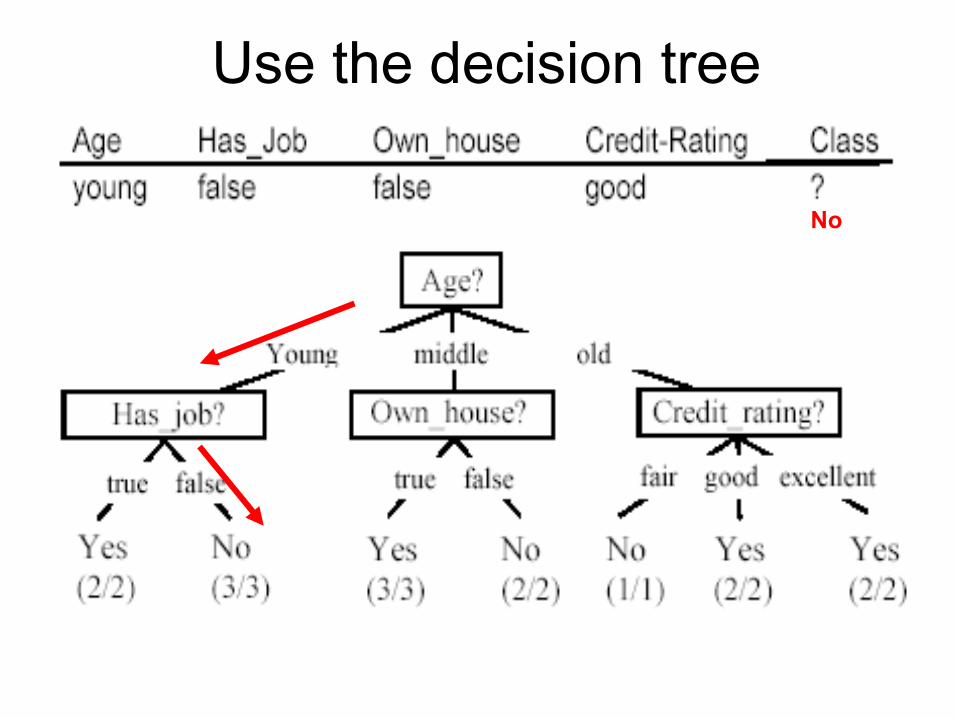
Use the decision tree

No

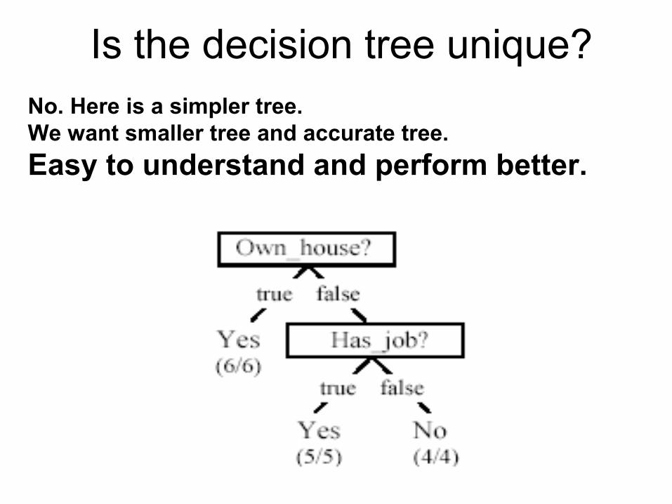
Is the decision tree unique?No. Here is a simpler tree. We want smaller tree and accurate tree.

Easy to understand and perform better.

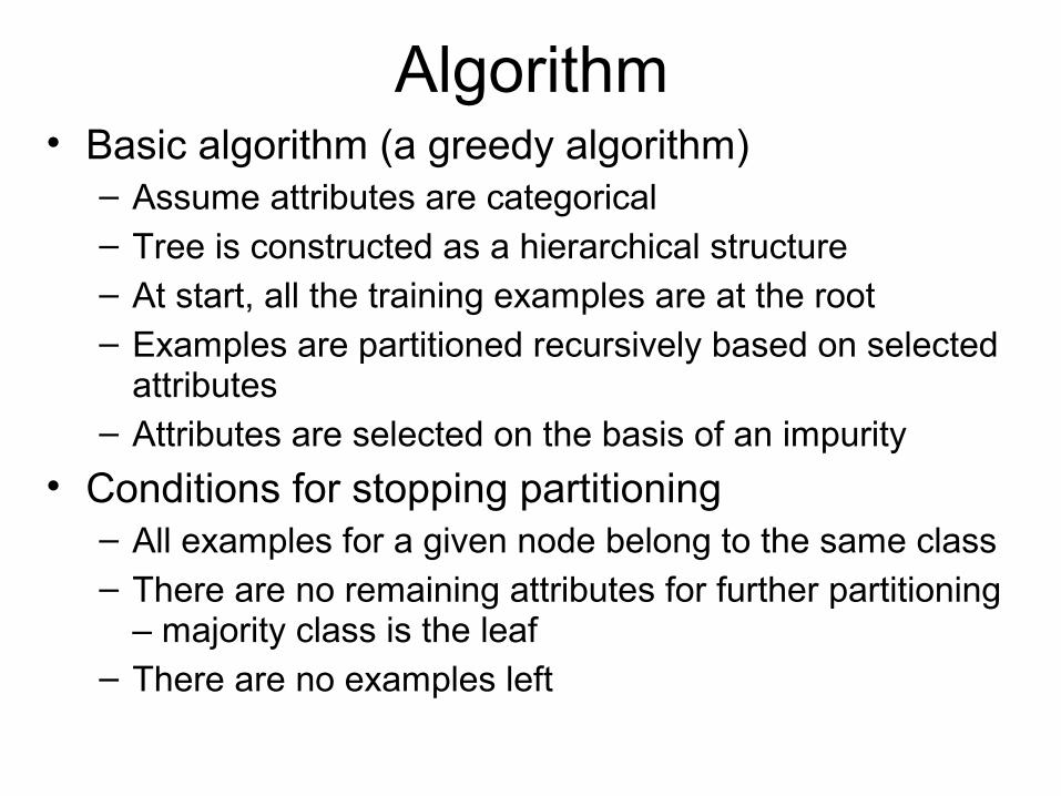
Algorithm• Basic algorithm (a greedy algorithm)

– Assume attributes are categorical– Tree is constructed as a hierarchical structure– At start, all the training examples are at the root– Examples are partitioned recursively based on selected

attributes– Attributes are selected on the basis of an impurity

• Conditions for stopping partitioning– All examples for a given node belong to the same class– There are no remaining attributes for further partitioning

– majority class is the leaf– There are no examples left

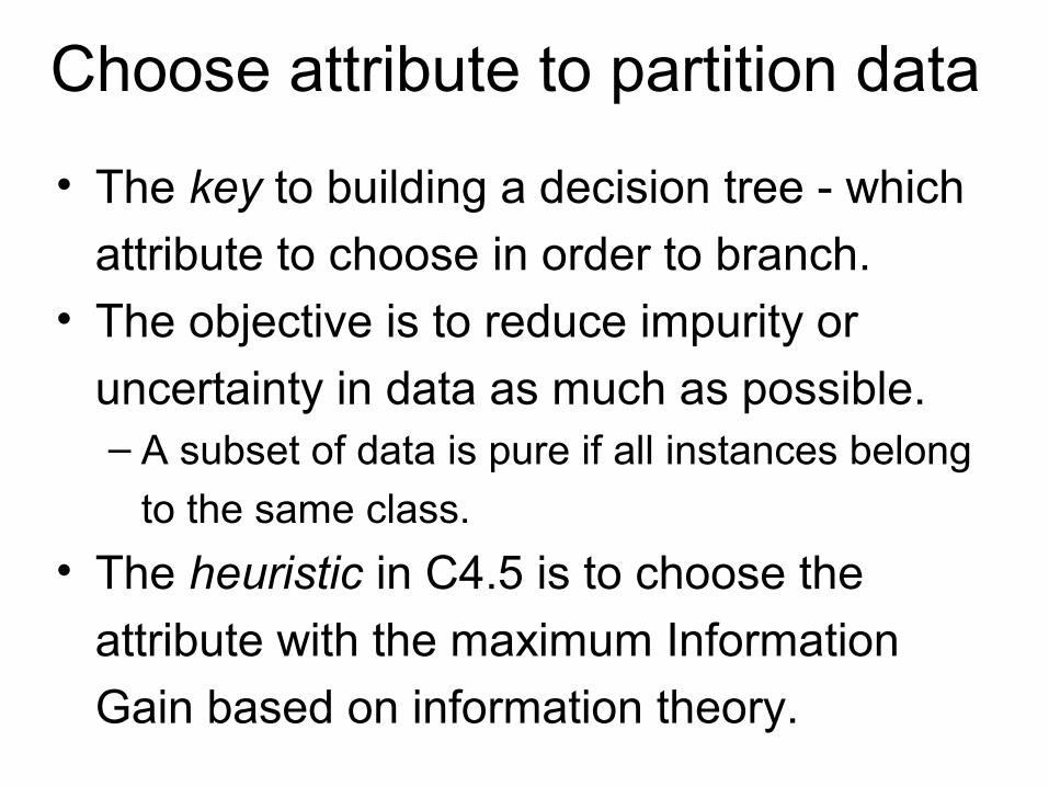
Choose attribute to partition data

• The key to building a decision tree - which

attribute to choose in order to branch. • The objective is to reduce impurity or

uncertainty in data as much as possible.– A subset of data is pure if all instances belong

to the same class.

• The heuristic in C4.5 is to choose the

attribute with the maximum Information

Gain based on information theory.

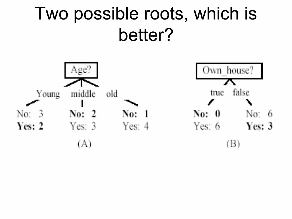
Two possible roots, which is better?

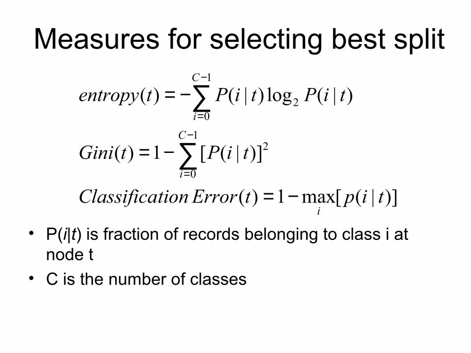
Measures for selecting best split

• P(i|t) is fraction of records belonging to class i at node t

• C is the number of classes

)]|([max1)(

)]|([1)(

)|(log)|()(

1

0

2

1

02

tiptErrortionClassifica

tiPtGini

tiPtiPtentropy

i

C

i

C

i

−=

−=

−=

∑

∑−

=

−

=

CS583, Bing Liu, UIC 44

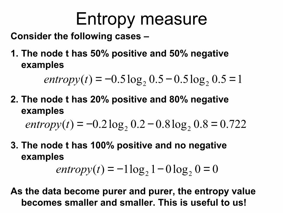
Entropy measureConsider the following cases –

1. The node t has 50% positive and 50% negative examples

2. The node t has 20% positive and 80% negative examples

3. The node t has 100% positive and no negative examples

As the data become purer and purer, the entropy value becomes smaller and smaller. This is useful to us!

15.0log5.05.0log5.0)( 22 =−−=tentropy

722.08.0log8.02.0log2.0)( 22 =−−=tentropy

00log01log1)( 22 =−−=tentropy

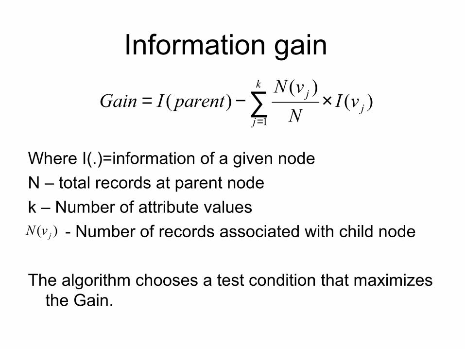
Information gain

Where I(.)=information of a given node

N – total records at parent node

k – Number of attribute values

- Number of records associated with child node

The algorithm chooses a test condition that maximizes the Gain.

∑=

×−=k

jj

j vIN

vNparentIGain

1

)()(

)(

)( jvN

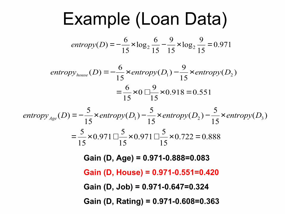
Example (Loan Data)

Gain (D, Age) = 0.971-0.888=0.083

Gain (D, House) = 0.971-0.551=0.420

Gain (D, Job) = 0.971-0.647=0.324

Gain (D, Rating) = 0.971-0.608=0.363

971.015

9log

15

9

15

6log

15

6)( 22 =×−×−=Dentropy

551.0918.015

90

15

6

)(15

9)(

15

6)( 21

=×+×=

×−×−= DentropyDentropyDentropyhouse

888.0722.015

5971.0

15

5971.0

15

5

)(15

5)(

15

5)(

15

5)( 321

=×+×+×=

×−×−×−= DentropyDentropyDentropyDentropyAge

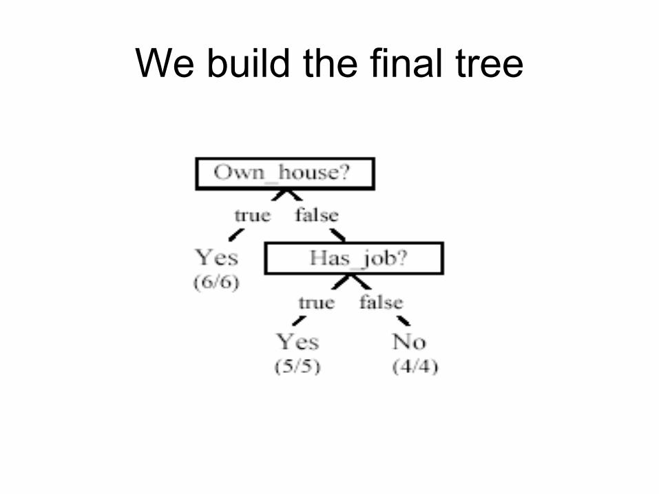
We build the final tree

Handling continuous attributes• Handle continuous attribute by splitting

into two intervals (can be more) at each node.

• How to find the best threshold to divide?– Use information gain again– Sort all the values of a continuous attribute in

increasing order {v1, v2, …, vr},

– One possible threshold between two adjacent values vi and vi+1. Try all possible thresholds and find the one that maximizes the gain.

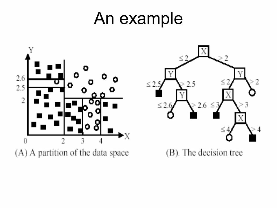
An example

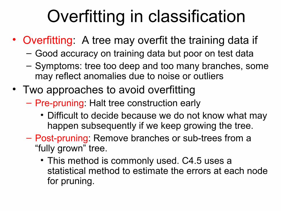
Overfitting in classification• Overfitting: A tree may overfit the training data if

– Good accuracy on training data but poor on test data– Symptoms: tree too deep and too many branches, some

may reflect anomalies due to noise or outliers

• Two approaches to avoid overfitting – Pre-pruning: Halt tree construction early

• Difficult to decide because we do not know what may happen subsequently if we keep growing the tree.

– Post-pruning: Remove branches or sub-trees from a “fully grown” tree.

• This method is commonly used. C4.5 uses a statistical method to estimate the errors at each node for pruning.

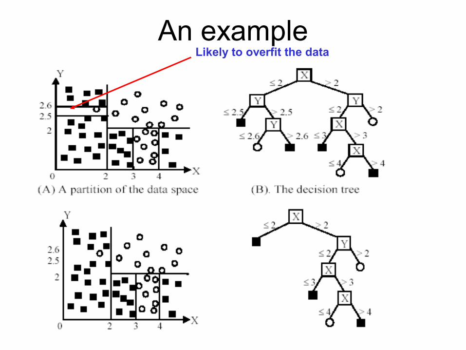
An exampleLikely to overfit the data