Modified clahe an adaptive algorithm for contrast enhancement of aerial medical and underwater images

International Journal of Computer Engineering and Technology (IJCET), ISSN 0976-6367(Print),

ISSN 0976 - 6375(Online), Volume 5, Issue 11, November (2014), pp. 32-47 © IAEME

32

MODIFIED CLAHE: AN ADAPTIVE ALGORITHM FOR

CONTRAST ENHANCEMENT OF AERIAL, MEDICAL

AND UNDERWATER IMAGES

Jharna Majumdar1, Santhosh Kumar K L

2

1Dean R&D, Prof& Head CSE (PG), Nitte Meenakshi Institute of Technology, Bangalore, India,

2Asst Prof, Dept. of CSE (PG), Nitte Meenakshi Institute of Technology, Bangalore, India,

ABSTRACT

Image enhancement has been an area of active research for decades. Most of the studies are

aimed at improving the quality of image for better visualization. Contrast Limited Adaptive

Histogram Equalization (CLAHE) is a technique to enhance the visibility of local details of an image

by increasing the contrast of local regions. The algorithm is extensively used by various researches

for applications in medical imagery. The drawback of CLAHE algorithm is the fact that it is not

automatic and needs two input parameters viz., N size of the sub window and CL the clip limit for

the method to work. Unfortunately none of the researchers have done the automatic selection of N

and CL to make the algorithm suitable for any autonomous system. This paper proposes a novel

extension of the conventional CLAHE algorithm, where N and CL are calculated automatically from

the given image data itself thereby making the algorithm fully adaptive. Our proposed algorithm is

used to study the enhancement of aerial, medical and underwater images. To demonstrate the

effectiveness of our algorithm, a set of quality metric parameters are used. In the conventional

CLAHE algorithm, we vary the value of N and CL and use the quality metric parameters to obtain

the best output for a given combination of N and CL. It is observed that for a given set input images,

the best results obtained using conventional CLAHE algorithm exactly matches with the results

obtained using our algorithm, where N and CL are calculated automatically.

Keywords: Image enhancement, Histogram Equalization, Contrast Limited Adaptive Histogram

Equalization, Adaptively Clipped Contrast Limited Adaptive Histogram Equalization (ACCLAHE),

Fully Automatic Contrast Limited Adaptive Histogram Equalization (Auto-CLAHE), Quality Metric

parameters.

INTERNATIONAL JOURNAL OF COMPUTER ENGINEERING &

TECHNOLOGY (IJCET)

ISSN 0976 – 6367(Print)

ISSN 0976 – 6375(Online)

Volume 5, Issue 11, November (2014), pp. 32-47

© IAEME: www.iaeme.com/IJCET.asp

Journal Impact Factor (2014): 8.5328 (Calculated by GISI)

www.jifactor.com

IJCET

© I A E M E



33

I. INTRODUCTION

Image enhancement, a well-known image preprocessing technique is used to improve the

appearance of an image and make it suitable for human visual perception or subsequent machine

learning. Commonly used image enhancement techniques fall into three different categories: (1)

Global enhancement (2) Local enhancement and (3) Adaptive Enhancement.

The paper consists of the following:

a) Adaptive enhancement techniques such as Adaptive Histogram Equalization [1], Contrast Limited

Adaptive Histogram Equalization (CLAHE) [1, 2] are widely used by researchers [3-6] [13-16]

b) We have proposed some modifications in the existing CLAHE algorithm and made it completely

adaptive and suitable for autonomous application. Proposed two new algorithms Adaptively Clipped

Contrast Limited Adaptive Histogram Equalization (ACCLAHE) and Fully Automatic Contrast

Limited Adaptive Histogram Equalization (AUTO CLAHE) are adaptive and completely suitable for

autonomous application.

c) We have studied the results of enhancement using a number of Quality Metric parameters.

d) We have used aerial, medical and underwater images for our experimental study and analysis of

results.

II. GLOBAL, LOCAL AND ADAPTIVE ENHANCEMENT METHODS

Histogram processing methods are global processing, in the sense that pixels are modified by

a transformation function based on the gray-level content of the entire image. An example of this is

Histogram Equalization. A local enhancement algorithm acts on local regions within an image. The

mapping applied on each pixel in the input image is decided upon by some property of the

neighborhood of that pixel. The methods vary from each other depending on the property chosen and

in the form in which it appears in the mapping. In such methods the size of the neighborhood or the

window size can be varied. Many enhancement algorithms require the user to choose some input

parameter(s) for enhancement. The enhancement is said to be adaptive, if the algorithm chooses the

optimum parameter(s) depending on the properties of the input image.

A. HISTOGRAM EQUALIZATION (HE)

Histogram equalization [5] is one of the well-known method for enhancing the contrast of

given images, making the result image have a uniform distribution of the gray levels. It flattens and

stretches the dynamic range of the image’s histogram and results in overall contrast improvement.

HE has been widely applied when the image needs enhancement however, it may significantly

change the brightness of an input image and cause problem in some applications where brightness

preservation is necessary. Since the HE is based on the whole information of input image to

implement, the local details with smaller probability would not be enhanced.

B. ADAPTIVE HISTOGRAM EQUALIZATION (AHE)

AHE is an extension to traditional Histogram Equalization technique. Unlike HE, it operates

on small data regions (tiles), rather than the entire image. The contrast of each region is enhanced, so

that the histogram of the output region approximately matches the specified histogram. The

neighboring regions are then combined using bilinear interpolation in order to eliminate artificially

induced boundaries [5]. In adaptive histogram equalization, the main idea is to take into account

histogram distribution over local window and combine it with global histogram distribution. The size

of the neighbourhood region is a parameter of the method. It constitutes a characteristic length scale:



34

contrast at smaller scales is enhanced, while contrast at larger scales is reduced. When the image

region containing a pixel's neighbourhood is fairly homogeneous, its histogram will be strongly

peaked, and the transformation function will map a narrow range of pixel values to the whole range

of the result image. This causes AHE to over amplify small amounts of noise in largely

homogeneous regions of the image [1].

C. CONTRAST LIMITED ADAPTIVE HISTOGRAM EQUALIZATION (CLAHE)

CLAHE is an adaptive contrast enhancement method. It is based on AHE, where the

histogram is calculated for the contextual region of a pixel. The pixel's intensity is thus transformed

to a value within the display range proportional to the pixel intensity's rank in the local intensity

histogram [1]. CLAHE, proposed by Zuierveld et al [2] has two key parameters: block size (N) and

clip limit (CL). These parameters are mainly used to control image quality, but have been

heuristically determined by users. CLAHE was originally developed for medical imaging [1].

CLAHE also had been claimed to improve the contrast better in the underwater [4, 12, and 13] and

aerial image enhancement [6].

III. THE PROPOSED METHODS

In this section, we describe two new proposed algorithms Adaptively Clipped Contrast

Limited Adaptive Histogram Equalization (ACCLAHE) and Fully Automatic Contrast Limited

Adaptive Histogram Equalization (Auto-CLAHE) in detail.

A. ADAPTIVELY CLIPPED CONTRAST LIMITED ADAPTIVE HISTOGRAM

EQUALIZATION (ACCLAHE)

We have found that the choice of clip limit is very crucial for optimal enhancement using

CLAHE. The correct choice of the clip level depends very much on the size of the bins in the local

histogram. In our proposed algorithm ACCLAHE, the estimation of the clip limit (CL) value is done

automatically from the given input image. We take the maximum bin height in the local histogram of

the sub-image and redistribute the clipped pixels equally to each gray-level. The ACCLAHE method,

however, is not fully automated as it still needs the value of N as a user input.

Algorithm 1: Adaptively Clipped Contrast Limited Adaptive Histogram Equalization(ACCLAHE) Input: Image file, N;

Output: ACCLAHE Enhanced Image;

STEPS:

1. Divide the input image into an NxN matrix of sub-images

2. For each sub-image do the following:

2.1 Compute the histogram of the sub-image

2.2 Compute the high peak value of the sub-image

2.3 Calculate the nominal clipping level, P from 0 to high peak using the binary search.

2.4 For each gray level bin in the histogram do the following:

(a) If the histogram bin is greater than the nominal clip level P, clip the histogram to the

nominal clip level P

(b) Collect the number of pixels in the sub-image that caused the histogram bin to exceed

the nominal clip level(P).

2.5 Distribute the clipped pixels uniformly in all histogram bins to obtain the renormalized

clipped histogram.



35

2.6 Equalize the above histogram to obtain the clipped HE mapping for the sub-image

3. For each pixel in the input image, do the following

3.1 If the pixel belongs to an internal region (IR), then

(a) Compute four weights, one for each of the four nearest sub-images, based on the

proximity of the pixel to the centers of the four nearest sub-images (nearer the center of

the sub-image, larger the weight ).

(b) Calculate the output mapping for the pixel as the weighted sum of the clipped HE

mappings for the four nearest sub-images using the weights computed above.

3.2 If the pixel belongs to an border region (BR), then

(a) Compute two weights, one for each of the two nearest sub-images, based on the

proximity of the pixel to the centers of the two nearest sub-images


mappings for the two nearest sub-images using the weights computed above.

3.3 If the pixel belongs to a corner region (CR), the output mapping for the pixel is the

clipped HE mapping for the sub-image that contains the pixel.

4. Apply the output mapping obtained to each of the pixels in the input image to obtain the image

enhanced by ACCLAHE.

B. FULLY AUTOMATIC CONTRAST LIMITED ADAPTIVE HISTOGRAM

EQUALIZATION (Auto-CLAHE)

We propose a method to fully automate the method of enhancement by estimating the value

of N from the global and local entropy in the input image. To each value of N, from N=2 (in which

case, the input image is divided into 2 x 2 = 4 sub-images) to N=12 (in which case, the input image

is divided into 12 x12 = 144 sub-images), we associate the maximum entropy over all the sub-

images of the same size. Now we choose that value of N that is associated with maximum entropy.

For the estimation of CL we follow the ACCLAHE method. We call this method of Auto CLAHE,

since both the input parameters N and CL are automatically estimated.

Algorithm 2: AUTO-CLAHE Input: Image file;

Output: AUTO-CLAHE Enhanced Image

STEPS:

1. For n=0 to n=12 store entropy[n] = 0.

2. For n = 2 to n = 12, divide the image into n x n matrix of sub-images and store the maximum

entropy of the 2n sub-images as entropy[n].

3. Set N to that value of n for which entropy[n] is maximum.

4. Divide the input image into an NxN matrix of sub-images

5. For each sub-image do the following:

5.1 Compute the histogram of the sub-image.

5.2 Compute the high peak value of the sub-image.

5.3 Calculate the nominal clipping level, P from 0 to high peak using the binary search

elaborated.

5.4 For each gray level bin in the histogram do the following

(a) If the histogram bin is greater than the nominal clip level P, clip the histogram to the

nominal clip level P

(b) Collect the number of pixels in the sub-image that caused the histogram bin to exceed

the nominal clip level.

5.5 Distribute the clipped pixels uniformly in all histogram bins to obtain the renormalized

clipped histogram.



36

5.6 Equalize the above histogram to obtain the clipped HE mapping for the sub-image

6. For each pixel in the input image, do the following

6.1 If the pixel belongs to an internal region (IR), then

(a) Compute four weights, one for each of the four nearest sub-images, based on the

proximity of the pixel to the centers of the four nearest sub-images (nearer the center of

the sub-image, larger the weight)


mappings for the four nearest sub-images using the weights computed above.

6.2 If the pixel belongs to an border region (BR), then

(a) Compute two weights, one for each of the two nearest sub-images, based on the

proximity of the pixel to the centers of the two nearest sub-images


mappings for the two nearest sub-images using the weights computed above.

6.3 If the pixel belongs to a corner region (CR), the output mapping for the pixel is the HE

mapping for the sub-image that contains the pixel.

7. Apply the output mapping obtained to each of the pixels in the input image to obtain the image

enhanced by Auto-CLAHE.

IV. EXPERIMENTAL STUDY, RESULTS & DISCUSSION

All the algorithms presented in this paper are implemented in the Windows 7 – Microsoft

Visual Studio platform using VC++ language for programming. The aerial, medical and underwater

images are selected for study. A set of quality metric parameters such as Entropy [7], Global

Contrast (GC) [8], Spatial Frequency (SF) [9], Fitness Measure (FM) [10] and Absolute Mean

Brightness Error (AMBE) [11] used to measure the quality of the enhanced image with respect to the

original image. The formulas of quality parameters are given in Appendix (section VIII).

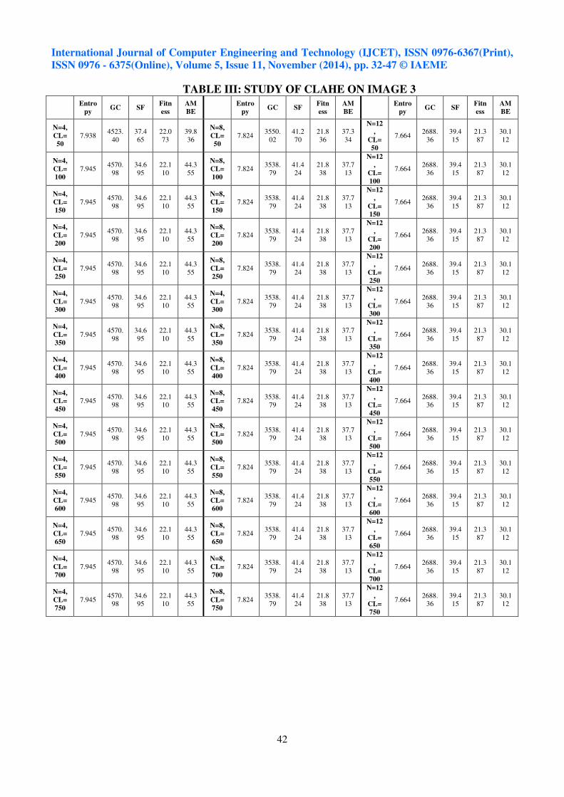
In Contrast Limited Adaptive Histogram Equalization (CLAHE), we have two input

parameters N and CL. The value of N is initially kept constant at N=4 and the value of CL is varied

from 50 to 750 in steps of 50. The experiment is repeated for the value of N=4, 8 and 12. Analysis of

the results show that for a given value of N as we increase the value of CL, after a certain value of

CL, all quality metric parameters reaches to saturation and remains constant throughout the scale as

shown in Table I,II,III and sample graphs shown for Global Contrast in Fig 13. The saturation value

of clip limit for a given image is not the same for all the values of N. It is seen that as we increase the

value of N, the optimum value of clip limit that gives the best enhancement result decreases as

evident from the Table IV. The reason may be attributed as follows: As we increase the value of N,

the size of the sub-image decreases. This implies a decrease in the number of pixels in the sub-image

and thus a lowering of the maximum bin height in the local histogram.

In the proposed “Adaptively Clipped Contrast Limited Adaptive Histogram Equalization”

(ACCLAHE) method, N is given as manual input and CL is estimated automatically. The value of N

is varied from 2 to 12 in steps of 2. It is seen from the Table V that the value of all quality

parameters increases initially and subsequently decreases after a certain value of N as shown for

Entropy and Fitness measure in Figs 14-15. The point where the quality parameters reaches

maximum value matches exactly with the saturation value obtained in CLAHE. This fact is observed

for all images used in our experiment.

In the proposed “Fully Automatic Contrast Limited Adaptive Histogram Equalization”

(Auto-CLAHE) method, the values of N and CL are estimated automatically. The effects of quality

metric parameters on the output image after enhancement are studied. It is seen that the saturation

value of CLAHE and ACCLAHE exactly matches with the results obtained using Auto-CLAHE as

shown in Table VI.



37

TABLE I : STUDY OF CLAHE ON IMAGE 1

Entro

py GC SF

Fitn

ess

AM

BE

Entro

py GC SF

Fitn

ess

AM

BE

Entro

py GC SF

Fitn

ess

AM

BE

N=4,

CL=

50

7.706 3260.

78

34.2

48

21.0

34

12.6

41

N=8,

CL=

50

7.687 3046.

91

38.5

03

21.2

51

16.5

12

N=12

,

CL=

50

7.484 2217.

28

35.9

58

20.7

45

15.1

00

N=4,

CL=

100

7.808 3924.

80 38.761

21.389

16.782

N=8,

CL=

100

7.731 3266.

07 41.128

21.394

18.803

N=12

,

CL=

100

7.514 2345.

89 38.177

20.852

17.115

N=4,

CL=

150

7.851 4203.

86

40.8

56

21.5

63

18.7

62

N=8,

CL=

150

7.740 3332.

79

42.3

32

21.4

35

20.2

22

N=12

,

CL=

150

7.521 2375.

86

38.8

63

20.8

78

17.8

76

N=4,

CL=

200

7.870 4328.

19

41.9

05

21.6

37

20.0

21

N=8,

CL=

200

7.746 3376.

53

43.0

73

21.4

53

21.0

51

N=12

,

CL=

200

7.521 2381.

29

39.0

19

20.8

79

18.0

90

N=4,

CL=

250

7.889 4414.

05

42.6

21

21.7

05

21.1

07

N=8,

CL=

250

7.748 3405.

58

43.5

41

21.4

86

21.4

95

N=12

,

CL=

250

7.522 2380.

94

39.0

55

20.8

81

18.2

03

N=4,

CL=

300

7.882 4403.

97

42.7

62

21.7

00

21.7

90

N=4,

CL=

300

7.749 3416.

85

43.7

66

21.4

99

21.7

42

N=12

,

CL=

300

7.522 2380.

94

39.0

55

20.8

81

18.2

03

N=4,

CL=

350

7.887 4429.

29

43.0

61

21.7

34

22.4

93

N=8,

CL=

350

7.749 3416.

81

43.8

31

21.5

01

21.8

86

N=12

,

CL=

350

7.522 2380.

94

39.0

55

20.8

81

18.2

03

N=4,

CL=

400

7.888 4441.

24

43.3

23

21.7

35

23.0

01

N=8,

CL=

400

7.749 3417.

34

43.8

65

21.5

02

21.9

52

N=12

,

CL=

400

7.522 2380.

94

39.0

55

20.8

81

18.2

03

N=4,

CL=

450

7.886 4456.

22

43.5

79

21.7

30

23.2

93

N=8,

CL=

450

7.749 3417.

34

43.8

65

21.5

02

21.9

52

N=12

,

CL=

450

7.522 2380.

94

39.0

55

20.8

81

18.2

03

N=4,

CL=

500

7.889 4459.

64

43.7

46

21.7

61

23.4

43

N=8,

CL=

500

7.749 3417.

34

43.8

65

21.5

02

21.9

52

N=12

,

CL=

500

7.522 2380.

94

39.0

55

20.8

81

18.2

03

N=4,

CL=

550

7.889 4462.

44

43.8

93

21.7

67

23.5

64

N=8,

CL=

550

7.749 3417.

34

43.8

65

21.5

02

21.9

52

N=12

,

CL=

550

7.522 2380.

94

39.0

55

20.8

81

18.2

03

N=4,

CL=

600

7.892 4474.

63

44.0

98

21.7

74

23.6

40

N=8,

CL=

600

7.749 3417.

34

43.8

65

21.5

02

21.9

52

N=12

,

CL=

600

7.522 2380.

94

39.0

55

20.8

81

18.2

03

N=4,

CL=

650

7.894 4484.

44 44.235

21.782

23.708

N=8,

CL=

650

7.749 3417.

34 43.865

21.502

21.952

N=12

,

CL=

650

7.522 2380.

94 39.055

20.881

18.203

N=4,

CL=

700

7.897 4505.

35

44.7

92

21.7

99

24.4

64

N=8,

CL=

700

7.749 3417.

34

43.8

65

21.5

02

21.9

52

N=12

,

CL=

700

7.522 2380.

94

39.0

55

20.8

81

18.2

03

N=4,

CL=

750

7.897 4505.

35

44.7

92

21.7

99

24.4

64

N=8,

CL=

750

7.749 3417.

34

43.8

65

21.5

02

21.9

52

N=12

,

CL=

750

7.522 2380.

94

39.0

55

20.8

81

18.2

03



38

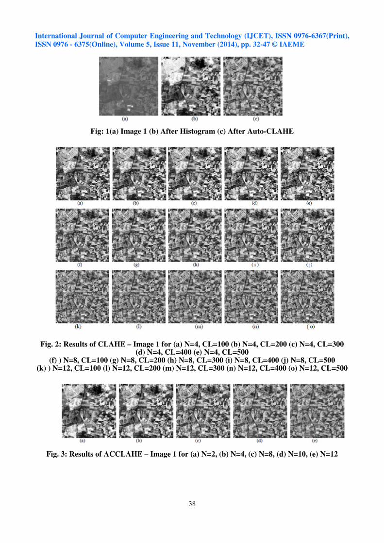
Fig: 1(a) Image 1 (b) After Histogram (c) After Auto-CLAHE

Fig. 2: Results of CLAHE – Image 1 for (a) N=4, CL=100 (b) N=4, CL=200 (c) N=4, CL=300

(d) N=4, CL=400 (e) N=4, CL=500 (f) ) N=8, CL=100 (g) N=8, CL=200 (h) N=8, CL=300 (i) N=8, CL=400 (j) N=8, CL=500

(k) ) N=12, CL=100 (l) N=12, CL=200 (m) N=12, CL=300 (n) N=12, CL=400 (o) N=12, CL=500

Fig. 3: Results of ACCLAHE – Image 1 for (a) N=2, (b) N=4, (c) N=8, (d) N=10, (e) N=12



39

TABLE II: STUDY OF CLAHE ON IMAGE 2

Entro

py GC SF

Fitn

ess

AM

BE

Entro

py GC SF

Fitn

ess

AM

BE

Entro

py GC SF

Fitn

ess

AM

BE

N=4,

CL=

50

7.851 3941.

46

38.8

42

22.0

53

26.8

89

N=8,

CL=

50

7.902 4128.

18

52.9

24

22.3

40

33.3

68

N=12

,

CL=

50

7.827 3684.

38

53.7

75

22.1

45

31.1

89

N=4,

CL=

100

7.855 4310.

29

47.0

78

22.1

39

33.3

82

N=8,

CL=

100

7.915 4337.

64

59.1

61

22.4

30

36.3

69

N=12

,

CL=

100

7.831 3726.

43

55.0

34

22.1

67

31.5

72

N=4,

CL=

150

7.891 4509.

31

52.2

66

22.2

81

36.0

89

N=8,

CL=

150

7.916 4416.

22

61.1

12

22.4

49

36.9

04

N=12

,

CL=

150

7.831 3726.

43

55.0

34

22.1

67

31.5

72

N=4,

CL=

200

7.892 4608.

05

55.1

46

22.3

11

37.7

65

N=8,

CL=

200

7.917 4418.

76

61.1

75

22.4

51

36.9

17

N=12

,

CL=

200

7.831 3726.

43

55.0

34

22.1

67

31.5

72

N=4,

CL=

250

7.873 4652.

37

56.8

80

22.2

73

38.6

89

N=8,

CL=

250

7.917 4418.

76

61.1

75

22.4

51

36.9

17

N=12

,

CL=

250

7.831 3726.

43

55.0

34

22.1

67

31.5

72

N=4,

CL=

300

7.878 4697.

98

58.3

36

22.3

03

39.2

91

N=4,

CL=

300

7.917 4418.

76

61.1

75

22.4

51

36.9

17

N=12

,

CL=

300

7.831 3726.

43

55.0

34

22.1

67

31.5

72

N=4,

CL=

350

7.877 4743.

86 59.636

22.311

39.724

N=8,

CL=

350

7.917 4418.

76 61.175

22.451

36.917

N=12

,

CL=

350

7.831 3726.

43 55.034

22.167

31.572

N=4,

CL=

400

7.889 4784.

01

60.7

20

22.3

55

40.0

52

N=8,

CL=

400

7.917 4418.

76

61.1

75

22.4

51

36.9

17

N=12

,

CL=

400

7.831 3726.

43

55.0

34

22.1

67

31.5

72

N=4,

CL=

450

7.889 4811.

81

61.5

21

22.3

61

40.3

46

N=8,

CL=

450

7.917 4418.

76

61.1

75

22.4

51

36.9

17

N=12

,

CL=

450

7.831 3726.

43

55.0

34

22.1

67

31.5

72

N=4,

CL=

500

7.876 4839.

44 62.227

22.329

40.513

N=8,

CL=

500

7.917 4418.

76 61.175

22.451

36.917

N=12

,

CL=

500

7.831 3726.

43 55.034

22.167

31.572

N=4,

CL=

550

7.887 4843.

79

62.3

15

22.3

62

40.5

12

N=8,

CL=

550

7.917 4418.

76

61.1

75

22.4

51

36.9

17

N=12

,

CL=

550

7.831 3726.

43

55.0

34

22.1

67

31.5

72

N=4,

CL=

600

7.887 4843.

81

62.3

15

22.3

62

40.5

11

N=8,

CL=

600

7.917 4418.

76

61.1

75

22.4

51

36.9

17

N=12

,

CL=

600

7.831 3726.

43

55.0

34

22.1

67

31.5

72

N=4,

CL=

650

7.887 4843.

81

62.3

15

22.3

62

40.5

11

N=8,

CL=

650

7.917 4418.

76

61.1

75

22.4

51

36.9

17

N=12

,

CL=

650

7.831 3726.

43

55.0

34

22.1

67

31.5

72

N=4,

CL=

700

7.887 4843.

81

62.3

15

22.3

62

40.5

11

N=8,

CL=

700

7.917 4418.

76

61.1

75

22.4

51

36.9

17

N=12

,

CL=

700

7.831 3726.

43

55.0

34

22.1

67

31.5

72

N=4,

CL=

750

7.887 4843.

81

62.3

15

22.3

62

40.5

11

N=8,

CL=

750

7.917 4418.

76

61.1

75

22.4

51

36.9

17

N=12

,

CL=

750

7.831 3726.

43

55.0

34

22.1

67

31.5

72



40

Fig: 4 (a) Image 2 (b) After Histogram (c) After Auto-CLAHE

Fig. 5: Results of CLAHE – Image 2 for (a) N=4, CL=100 (b) N=4, CL=200 (c) N=4, CL=300 (d) N=4, CL=400 (e) N=4, CL=500

(f) ) N=8, CL=100 (g) N=8, CL=200 (h) N=8, CL=300 (i) N=8, CL=400 (j) N=8, CL=500 (k) ) N=12, CL=100 (l) N=12, CL=200 (m) N=12, CL=300 (n) N=12, CL=400 (o) N=12, CL=500

Fig. 6: Results of ACCLAHE – Image 2 for (a) N=2, (b) N=4, (c) N=8, (d) N=10, (e) N=12



41

Fig: 7 (a) Image 3 (b) After Histogram (c) After Auto-CLAHE

Fig. 8: Results of CLAHE – Image 3 for (a) N=4, CL=100 (b) N=4, CL=200 (c) N=4, CL=300

(d) N=4, CL=400 (e) N=4, CL=500

(f) ) N=8, CL=100 (g) N=8, CL=200 (h) N=8, CL=300 (i) N=8, CL=400 (j) N=8, CL=500

(k) ) N=12, CL=100 (l) N=12, CL=200 (m) N=12, CL=300 (n) N=12, CL=400 (o) N=12, CL=500

FIG. 9: RESULTS OF ACCLAHE – IMAGE 3 FOR (A) N=2, (B) N=4, (C) N=8, (D) N=10, (E) N=12



42

TABLE III: STUDY OF CLAHE ON IMAGE 3

Entro

py GC SF

Fitn

ess

AM

BE

Entro

py GC SF

Fitn

ess

AM

BE

Entro

py GC SF

Fitn

ess

AM

BE

N=4,

CL=

50

7.938 4523.

40

37.4

65

22.0

73

39.8

36

N=8,

CL=

50

7.824 3550.

02

41.2

70

21.8

36

37.3

34

N=12

,

CL=

50

7.664 2688.

36

39.4

15

21.3

87

30.1

12

N=4,

CL=

100

7.945 4570.

98

34.6

95

22.1

10

44.3

55

N=8,

CL=

100

7.824 3538.

79

41.4

24

21.8

38

37.7

13

N=12

,

CL=

100

7.664 2688.

36

39.4

15

21.3

87

30.1

12

N=4,

CL=

150

7.945 4570.

98

34.6

95

22.1

10

44.3

55

N=8,

CL=

150

7.824 3538.

79

41.4

24

21.8

38

37.7

13

N=12

,

CL=

150

7.664 2688.

36

39.4

15

21.3

87

30.1

12

N=4,

CL=

200

7.945 4570.

98

34.6

95

22.1

10

44.3

55

N=8,

CL=

200

7.824 3538.

79

41.4

24

21.8

38

37.7

13

N=12

,

CL=

200

7.664 2688.

36

39.4

15

21.3

87

30.1

12

N=4,

CL=

250

7.945 4570.

98

34.6

95

22.1

10

44.3

55

N=8,

CL=

250

7.824 3538.

79

41.4

24

21.8

38

37.7

13

N=12

,

CL=

250

7.664 2688.

36

39.4

15

21.3

87

30.1

12

N=4,

CL=

300

7.945 4570.

98

34.6

95

22.1

10

44.3

55

N=4,

CL=

300

7.824 3538.

79

41.4

24

21.8

38

37.7

13

N=12

,

CL=

300

7.664 2688.

36

39.4

15

21.3

87

30.1

12

N=4,

CL=

350

7.945 4570.

98

34.6

95

22.1

10

44.3

55

N=8,

CL=

350

7.824 3538.

79

41.4

24

21.8

38

37.7

13

N=12

,

CL=

350

7.664 2688.

36

39.4

15

21.3

87

30.1

12

N=4,

CL=

400

7.945 4570.

98

34.6

95

22.1

10

44.3

55

N=8,

CL=

400

7.824 3538.

79

41.4

24

21.8

38

37.7

13

N=12

,

CL=

400

7.664 2688.

36

39.4

15

21.3

87

30.1

12

N=4,

CL=

450

7.945 4570.

98 34.695

22.110

44.355

N=8,

CL=

450

7.824 3538.

79 41.424

21.838

37.713

N=12

,

CL=

450

7.664 2688.

36 39.415

21.387

30.112

N=4,

CL=

500

7.945 4570.

98

34.6

95

22.1

10

44.3

55

N=8,

CL=

500

7.824 3538.

79

41.4

24

21.8

38

37.7

13

N=12

,

CL=

500

7.664 2688.

36

39.4

15

21.3

87

30.1

12

N=4,

CL=

550

7.945 4570.

98

34.6

95

22.1

10

44.3

55

N=8,

CL=

550

7.824 3538.

79

41.4

24

21.8

38

37.7

13

N=12

,

CL=

550

7.664 2688.

36

39.4

15

21.3

87

30.1

12

N=4,

CL=

600

7.945 4570.

98

34.6

95

22.1

10

44.3

55

N=8,

CL=

600

7.824 3538.

79

41.4

24

21.8

38

37.7

13

N=12

,

CL=

600

7.664 2688.

36

39.4

15

21.3

87

30.1

12

N=4,

CL=

650

7.945 4570.

98

34.6

95

22.1

10

44.3

55

N=8,

CL=

650

7.824 3538.

79

41.4

24

21.8

38

37.7

13

N=12

,

CL=

650

7.664 2688.

36

39.4

15

21.3

87

30.1

12

N=4,

CL=

700

7.945 4570.

98

34.6

95

22.1

10

44.3

55

N=8,

CL=

700

7.824 3538.

79

41.4

24

21.8

38

37.7

13

N=12

,

CL=

700

7.664 2688.

36

39.4

15

21.3

87

30.1

12

N=4,

CL=

750

7.945 4570.

98

34.6

95

22.1

10

44.3

55

N=8,

CL=

750

7.824 3538.

79

41.4

24

21.8

38

37.7

13

N=12

,

CL=

750

7.664 2688.

36

39.4

15

21.3

87

30.1

12



43

TABLE IV. SATURATION POINTS IN CLAHE METHOD FOR TEST IMAGES

TABLE V. STUDY OF ACCLAHE ON TEST IMAGES

IMAGE 1 IMAGE 2 IMAGE 3

Entropy GC SF Fitness AMBE Entropy GC SF Fitness AMBE Entropy GC SF Fitness AMBE

N=2 7.735 4960.00 43.308 21.001 25.068 7.707 5131.02 49.538 21.696 41.857 7.951 5047.09 38.682 22.042 45.920

N=4 7.897 4505.35 44.792 21.799 24.464 7.887 4843.81 62.315 22.362 40.511 7.945 4570.98 34.695 22.110 44.355

N=6 7.831 4009.16 44.513 21.630 22.799 7.933 4745.58 62.499 22.500 39.758 7.889 4010.07 41.355 22.010 42.161

N=8 7.749 3417.34 43.865 21.502 21.952 7.917 4418.54 61.172 22.451 36.916 7.824 3538.79 41.424 21.838 37.713

N=10 7.636 2861.22 41.431 21.210 19.482 7.879 4104.29 58.612 22.325 34.592 7.745 3083.33 40.419 21.611 33.982

N=12 7.522 2380.94 39.055 20.881 18.203 7.831 3726.32 55.031 22.167 31.572 7.664 2688.36 39.415 21.387 30.112

TABLE VI. STUDY OF ACCLAHE ON TEST IMAGES

IMAGE 1 IMAGE 2 IMAGE 3 (fish image)

Entropy GC SF Fitness AMBE Entropy GC SF Fitness AMBE Entropy GC SF Fitness AMBE

Original

Image 4.898 346.85 9.458 12.554 - 6.450 1752.12 15.719 17.471 - 7.230 1465.29 16.694 19.642 -

Saturation

value of

CLAHE

7.897 4505.35 44.792 21.799 24.464 7.887 4843.81 62.315 22.362 40.511 7.951 5047.09 34.682 22.042 45.920

ACCLAHE

Image 7.897 4505.35 44.792 21.799 24.464 7.887 4843.81 62.315 22.362 40.511 7.951 5047.09 34.682 22.042 45.920

Auto-

CLAHE

Image

7.897 4505.35 44.792 21.799 24.464 7.887 4843.81 62.315 22.362 40.511 7.951 5047.09 34.682 22.042 45.920

Parameters Image 1 Image 3 Image3

N 4 8 12 4 8 12 4 8 12

CL 700 400 250 600 200 100 100 100 50



44

Fig. 13: Effect of Global Contrast on CLAHE for different N values

Fig.14.Effect of Entropy on ACCLAHE Fig.15 Effect of Entropy on ACCLAHE

for three sample images for three sample images

V. CONCLUSION

The aim of our research is to make the algorithm automatic and adaptive with no manual

input. The value of N and CL are estimated automatically from the given image data, thereby making

the algorithm applicable in any autonomous system. In the existing CLAHE, it is observed that for a

given value of N as we increase the value of CL, we get the values of all quality metric parameters

which remain constant for further change in the value of CL. We have termed this as ‘Saturation

Value’.

In the proposed ACCLAHE and Auto-CLAHE, we get a set of quality metric parameters for

a given input image which exactly matches with the ‘saturation values’ obtained in CLAHE. We

have also analyzed the methodology used to evaluate the algorithms’ performance, highlighting the

works where a quantitative quality metric has been used.



45

VI. ACKNOWLEDGMENTS

The authors express their sincere gratitude to Prof. N R Shetty, Director, Nitte Meenakshi

Institute of Technology and Dr. H C Nagaraj, Principal, Nitte Meenakshi Institute of Technology for

providing encouragement, support and the infrastructure to carry out the research.

VII. REFERENCES

[1] Stephen M. Pizer, E. Philip Amburn, John D. Austin, Robert Cromartie, “Adaptive Histogram

Equalization and Its Variations,” Computer Vision, Graphics, And Image Processing 39, 355-

368 (1987)

[2] K. Zuiderveld, “Contrast Limited Adaptive Histogram Equalization”, Academic Press Inc.,

(1994).

[3] Kashif Iqbal, Rosalina Abdul Salam, azam Osman and Abdullah Zawawi Talib, “Underwater

Image Enhancement Using an Integrated Colour Model,” IAENG International Journal of

Computer Science, 34:2, IJCS_34_2_12, 2007

[4] Balvant Singh, Ravi Shankar Mistra, Puran Gour, “Analysis of Contrast Enhancement

Techniques For Underwater Image,” IJCTEE Volume 1, Issue 2, 2009

[5] Rajesh Garg, Bhawna Mittal, sheetal garg, “Histogram Equalization Techniques For Image

Enhancement,” International Journal of Electronics & Communication Technology, Volume 2,

Issue 1, March 2011

[6] Ramyashree N, Pathra P, Shruthi T V, Dr. JharnaMajumdar, “Enhacement of Aerial and

Medical Image using Multi resolution pyramid,” Special Issue of IJCCT Vol. 1 Issue 2,3,4;

International Conferecnce - ACCTA-2010

[7] Zhengmao Ye, Objective Assessment of Nonlinear Segmentation Approaches to Gray Level

Underwater Images, ICGST-GVIP Journal, ISSN 1687-398X, Volume (9), Issue (II), April

2009

[8] Jia-Guu Leu, “Image Contrast Enhancement Based on the Intensities of Edge Pixels,”

CVGIP: Graphical Models And Image Processing Vol. 54, No. 6, November, pp. 497-506,

1992.

[9] Sonja Grgi c Mislav Grgic Marta Mrak, “Reliability of Objective Picture Quality Measures,”

Journal of ELECTRICAL ENGINEERING, VOL. 55, NO. 1-2, 2004, 3-10.

[10] Munteanu C and Rosa A, “Gray-Scale Image Enhancement as an Automatic Process Driven

by Evolution,” IEEE Transactions on Systems, Man, and Cybernetics—Part B: Cybernetics,

Vol. 34, No. 2, April 2004.

[11] Iyad Jafar Hao Ying, “A New Method for Image Contrast Enhancement Based on Automatic

Specification of Local Histograms”, IJCSNS International Journal of Computer Science and

Network Security, VOL.7 No.7, July 2007.

[12] Raimondo Schettini and Silvia Corchs, “Review Article - Underwater Image Processing :

State of the Art of restoration and Image Enhancement Methods,” EURASIP Journal on

Advances in Signal Processing, Volume 2010.

[13] Rajesh Kumar Rai, Puran Gour, Balvant Singh, “Underwater Image Segmentation using

CLAHE Enhancement and Thresholding,” International Journal of Emerging Technology and

Advanced Engineering, ISSN 2250-2459, Volume 2, Issue 1, January 2012

[14] Wan Nural Jawahir Hj Wan Yussof, Muhammad Suzuri Hitam, Ezmahamrul Afreen

Awalludin, and Zainuddin Bachok, “Performing Contrast Limited Adaptive Histogram

Equalization Technique on Combined Color Models for Underwater Image Enhancement,”

International Journal of Interactive Digital Media, Vol. 1(1), ISSN 2289-4098, e-ISSN 2289-

4101- 2013



46

[15] D. P. Sharma “Intensity Transformation using Contrast Limited Adaptive Histogram

Equalization” International Journal of Engineering Research (ISSN: 2319-6890) Volume

No.2, Issue No. 4, pp : 282-285 01 Aug. 2013

[16] Neethu M. Sasi, V. K. Jayasree, “ Contrast Limited Adaptive Histogram Equalization for

Qualitative Enhancement of Myocardial Perfusion Images,” Scientific Research, October

2013

[17] Prathap P and Manjula S, “To Improve Energy-Efficient and Secure Multipath

Communication In Underwater Sensor Network” International journal of Computer

Engineering & Technology (IJCET), Volume 5, Issue 2, 2014, pp. 145 - 152, ISSN Print:

0976 – 6367, ISSN Online: 0976 – 6375.

VIII. APPENDIX : QUALITY METRIC PARAMETERS FOR IMAGE ENHANCEMENT

A. ENTROPY:

The entropy [7] also called discrete entropy is a measure of information content in an image

and is given by,

∑=−=

255

0 2 ))((log)(k

kpkpEntropy (1)

Where p(k) is the probability distribution function. Larger the entropy, larger is the information

contained in the image and hence more details are visible in the image.

B. GLOBAL CONTRAST (GC):

The global contrast [8] value of an image is defined as the second central moment of its

histogram divided by N, the total number of pixels in the image.

N

ihistiGC

L

i∑=−

=0

2 )(*)( µ

(2)

Where, µ is the average intensity of the image, hist(i) is the number of pixels in the image with the

intensity value i and L is the highest intensity value.

C. SPATIAL FREQUENCY(SF): The Spatial Frequency [9] indicates the overall activity level in an image. SF is defined as

follows:

22CRSF += (3)

2

1 2

1,, )(1∑∑

= =

−−=

M

j

N

k

kjkj xxMN

R (4)

2

1 2

,1, )(1∑∑

= =

−−=

M

k

N

j

kjkj xxM

C (5)



47

Where R is row frequency, C is column frequency and xj,k denotes the pixel intensity values of

image; M and N are numbers of pixels in horizontal and vertical directions.

D. FITNESS MEASURE: The Fitness measure [10] depends on the entropy H(I), no. of edges n(I) and the intensity of

edges E(I).

)()*(

)())(ln(ln IH

heightwidth

IneIEsureFitnessMea +=

(6)

Compared to the original image, the enhanced version should have a higher intensity of the edges.

E. ABSOLUTE MEAN BRIGHTNESS ERROR (AMBE): AMBE [11] simply measures the deviation of the processed image mean ‘µp’ from the input

image mean ‘µi’

ipAMBE µµ −= (7)

The AMBE value provides a sense of how the image global appearance has changed, with

preference to lower values.