Embed Size (px)
Citation preview

Lecture Notes in Earth Sciences 103Editors:S. Bhattacharji, BrooklynH. J. Neugebauer, BonnJ. Reitner, GöttingenK. Stüwe, Graz
Founding Editors:G. M. Friedman, Brooklyn and TroyA. Seilacher, Tübingen and Yale

3BerlinHeidelbergNew YorkHong KongLondonMilanParisTokyo
Michael Kühn
123
Reactive Flow Modelingof Hydrothermal Systems
With 68 Colour Illustrations
Author
Dr. Michael KühnCSRIO – ARRC / Exploration and Mining26 Dick Perry Avenue, Technology ParkKensington, Perth, WA 6151Australia
This work is subject to copyright. All rights are reserved, whether the whole or part of the materialis concerned, specifically the rights of translation, reprinting, re-use of illustrations, recitation,broadcasting, reproduction on microfilms or in any other way, and storage in data banks. Duplicationof this publication or parts thereof is permitted only under the provisions of the German CopyrightLaw of September 9, 1965, in its current version, and permission for use must always be obtainedfrom Springer-Verlag. Violations are liable for prosecution under the German Copyright Law.
Springer-Verlag is a part of Springer Science+Business Media
springeronline.com
© Springer-Verlag Berlin Heidelberg 2004Printed in Germany
The use of general descriptive names, registered names, trademarks, etc. in this publication does notimply, even in the absence of a specific statement, that such names are exempt from the relevantprotective laws and regulations and therefore free for general use.
Cover design: Erich Kirchner, HeidelbergTypesetting: Camera ready by authorPrinted on acid-free paper 32/3142/du - 5 4 3 2 1 0
ISSN 0930-0317ISBN 3-540-20338-9 Springer-Verlag Berlin Heidelberg New York
Cataloging-in-Publication Data applied for
Bibliographic information published by Die Deutsche Bibliothek.Die Deutsche Bibliothek lists this publication in the Deutsche Nationalbibliographie; detailedbibliographic data is available in the Internet at <http://dnb.ddb.de>.
”For all Lecture Notes in Earth Sciences published till now please see final pagesof the book“
Preface
This book introduces the topic of geochemical reaction modeling of the fluids in
subsurface and hydrothermal systems. It is designed for readers first entering into
this world as well as for sophisticated researchers who want to improve their
knowledge especially of the interaction between chemical reactions and other
processes like fluid flow and heat transfer in hydrothermal systems. Furthermore,
it will be of interest for characterization, delineation, and exploration of geother-
mal reservoirs as well as for mineral geology, to explain or to reassess existing
deposits and to search for new ones.
The intention behind this manuscript has been to serve as a textbook for gradu-
ate students in aqueous, environmental, and groundwater geochemistry, despite
the fact that its focus is on the special topic of geochemistry in hydrothermal sys-
tems, and to provide new insights for experienced researches with respect to the
topic of reactive transport. The overall purpose of the book is to give the reader an
understanding of the processes that control the chemical composition of waters in
hydrothermal systems and to point out the interfaces between chemistry, geother-
mics, and hydrogeology.
The first chapter displays the significance of geochemical models of hydro-
thermal systems and their use in reservoir exploration and exploitation. It outlines
the objectives of this book and the conducted research work.
The second chapter consists of two parts. The first part explains main concepts
of different types of geothermal systems. Particular attention is given to chemical,
physical, and geometric features. In the second part different types of water exist-
ing in geothermal reservoirs worldwide are reviewed. Their compositions are dis-
cussed and related to the basic processes that dominate their chemistry.
In the third chapter geochemical modeling theories are presented in a sequence
of increasing complexity from geochemical equilibrium models to kinetic, reac-
tion path, and finally coupled transport and reaction models. The state of the art of
hydrothermal reactive transport simulation is delineated. Available numerical
codes are presented, which are capable to simulate the processes fluid flow, heat
transfer, transport, and chemical reactions, necessary for a comprehensive study of
hydrothermal systems. Uncertainty, usefulness, and limitations of hydrogeochemi-
cal models are discussed in general.
In the fourth chapter specific features of coupled fluid flow and chemical reac-
tion are investigated in more detail. Distinct types of reactive environments are
described in combination with permeability-porosity relationships resulting in
specific flow induced reaction patterns. The specific phenomena of reactive infil-
tration instability and free thermal convection are investigated accordingly.
VI Preface
Reactive transport modeling of the history of fossil hydrothermal systems is
presented in the fifth chapter. Firstly, a brief overview is given about numerical
simulations done to investigate genesis of ore deposits as well as progress of
diagenetic processes. Secondly, a detailed examination of formation scenarios is
presented in order to understand the observed anhydrite cementation at the loca-
tion Allermöhe (Germany). This is done under special consideration of the recent
structure of the Allermöhe site and its geological history.
Aim of numerical investigations of recent hydrothermal systems in chapter six
is to set-up or to evaluate conceptual models of geothermal areas. Within the first
part of this chapter some of the currently published numerical studies are summa-
rized. The following second part is a detailed case study of the shallow hydro-
thermal system of Waiwera (New Zealand), investigating the complex interaction
of density driven flow, heat transfer, and chemical reactions.
In chapter seven opportunities are discussed of the application of reactive
transport modeling for reservoir management purposes. The case study of the long
term performance of the geothermal potential Stralsund (Germany) is shown in
detail.
For the interested reader a CD-ROM is available from the author, which in-
cludes the complete database of the geothermal waters compiled from an exten-
sive literature study (Chap. 2, readable with MS Access ) and all numerical mod-
els presented here (Chap. 4 to 7) with a comprehensive selection of the produced
results. The models may be investigated with the help of either Processing
SHEMAT (Clauser 2003, available at Springer Publishers, Berlin-Heidelberg) or
the SHEMAT Viewer (provided with the CD-ROM).
Finally, the reader must note that I take full responsibility for the contents of
this book. If some of the theories and concepts taken from the literature are misin-
terpreted, this was unintentional and does not reflect disregard of the original au-
thor's work.
Acknowledgements
My thanks go to the German Federal Ministry for Education, Science, Research,
and Technology (BMBF) and the German Federal Ministry for Economic Affairs
(BMWi) for the financial support during the past five years. The contents of the
work in hand arose in the context of the projects “Hydraulic, thermal and me-
chanical behavior of geothermally used aquifers” (BMBF, under grant 032 69 95)
and “Scenarios of the Emergence of Anhydrite Cementation in Geothermal Reser-
voirs” (BMWi, under grant 032 70 95).
When a work like this is produced over a long period of time, it is difficult to
limit the acknowledgements as many people have contributed in different ways.
However, I should first like to thank Prof. Dr.-Ing. Wilfried Schneider who en-
gaged me at the TU Hamburg-Harburg and who encouraged me to write this book
and provided moral support and valuable discussions. I am thankful for his confi-
dence in my work and the freedom he allowed me to guide the "Geothermal" pro-
jects in my sole discretion.
Preface VII
I would like to thank Prof. Dr.-Ing. Knut Wichmann who affiliated me in the
Department of Water Management and Water Supply at the Technical University
of Hamburg-Harburg. He provided any support I needed for my research work.
Thanks to all my colleagues and friends from the Department, who gave me a
helping hand when I needed one and who readily shared their computer with me
when I needed more computational power.
I am indebted to a number of people. Special thanks go to Dr. Jörn Bartels who
had great stake in my employment at the TU Hamburg-Harburg and I appreciate
his advice during the learning of computer programming. His endless input and
critical discussions were invaluable for the "fully coupling" of his physical and my
geochemical ideas and experiences.
I would like to express my sincere gratitude to Dipl.-Ing. Heinke Stöfen for her
continuing support as collegiate assistant, diploma student, and colleague and for
the fruitful discussions we had.
I am thankful for adjuvant suggestions and efforts of Prof. Dr. Christoph
Clauser. Furthermore, I am grateful to Dr. Hansgeorg Pape, Dipl.-Geol. Joachim
Iffland, and Dr. Andreas Günther for their geological and petrophysical input and
explanations.
I am much obliged to Prof. Patrick R.L. Browne, Prof. Arnold Watson, and the
whole staff of the Geothermal Institute at the University of Auckland for their
warm welcome, help and advices during my stays in New Zealand in 1999 and
2001. Moreover I am thankful for the all-embracing support of Stephen Crane
from the Auckland Regional Council concerning the Waiwera geothermal field
(New Zealand) and the help of Francisco da Costa Monteiro during my field stud-
ies at Waiwera.
Furthermore I am grateful to Dr. Jörn Bartels, Dr. Martin Kölling, Dr. Paul
Hoskin, Dipl.-Ing. Heinke Stöfen, and Dipl.-Ing. Thomas Nuber for finding time
in busy schedules to help with reviewing the manuscript. Various drafts were im-
proved immensely thanks to their vigilant proofreading.
Thanks also due to ITA Jens-Uwe Stoß, who assisted with several graphics, and
to Ulrike Witt and Ciprian Scurtu for build up of the geothermal water database.
Throughout all this time however, my greatest supporter and source of encour-
agement and love has been Silke Gößling. Finally I would like to thank her, my
children Lisa and Lukas, and my family and friends for moral support and for
allowing me to use my free time to finish this book.
Michael Kühn

Contents
1 General Significance of Geochemical Models of Hydrothermal Systems......1
1.1 Fossil and Recent Hydrothermal Systems.....................................................4
1.2 Hydrogeothermal Energy Use .......................................................................5
1.3 Reservoir Exploration and Management.......................................................7
1.4 Geochemical Models .....................................................................................8
2 Concepts, Classification, and Chemistry of Geothermal Systems ................11
2.1 Conceptual Model and Classification..........................................................11
2.2 Static – Conductive Systems .......................................................................14
2.2.1 Magmatic Systems ...............................................................................14
2.2.2 Sediment Hosted Systems....................................................................14
2.3 Dynamic – Convective Systems ..................................................................15
2.3.1 Magmatic - High-Temperature ............................................................15
2.3.2 Sediment Hosted - Low-Temperature..................................................21
2.4 Geothermal Water Compilation...................................................................23
2.5 Chemical Interpretation of Geothermal Waters ..........................................26
2.5.1 Thermal Water Types...........................................................................27
2.5.2 Graphical Interpretation Methods ........................................................28
2.6 Processes Affecting the Chemical Composition of Hydrothermal Waters 33
2.6.1 Dynamic Magmatic Systems (High-Temperature) .............................33
2.6.2 Static and Dynamic Sediment Hosted Systems (Low Temperature) ..39
2.7 Geothermometer ..........................................................................................40
3 Theory of Chemical Modeling...........................................................................47
3.1 Geochemical Equilibrium............................................................................47
3.1.1 Activity Calculations and Solubility of Minerals................................48
3.1.2 Comparison of Ion Activity Calculation Methods ..............................52
3.1.3 Batch Models........................................................................................53
3.2 Kinetic Models.............................................................................................54
3.3 Reaction Pathways .......................................................................................56
X Contents
3.3.1 Polythermal Reaction Models..............................................................57
3.3.2 Titration Models ...................................................................................57
3.3.3 System Open to External Gas Reservoirs ............................................58
3.3.4 Flow-Through Reaction Path ...............................................................58
3.3.5 Reaction Path Models Applied to Hydrothermal Systems..................59
3.4 Simulation of Transport and Reaction.........................................................61
3.4.1 Groundwater Flow................................................................................61
3.4.2 Solute Transport ...................................................................................71
3.4.3 Heat Transport......................................................................................75
3.4.4 State of the Art of Hydrothermal Reactive Transport Simulation ......77
3.5 Uncertainty, Usefulness, and Limitations of Models..................................79
4 Specific Features of Coupled Fluid Flow and Chemical Reaction................81
4.1 Flow Induced Reaction Patterns ..................................................................82
4.1.1 Flow Across Mineralogical Boundaries ..............................................82
4.1.2 Moving Reaction Fronts.......................................................................83
4.1.3 Reactions Within Thermal Gradients ..................................................84
4.1.4 Mixing Zone Environments .................................................................85
4.1.5 Local Flow Enhancement due to Faults...............................................86
4.2 Porosity and Permeability (Reduction) Models ..........................................86
4.3 Reactive Infiltration Instability....................................................................90
4.3.1 Peclet and Damköhler Number............................................................91
4.3.2 Example of Preferential Flow Path Development ...............................92
4.3.3 Parameter Analysis of Reaction Front Instabilities .............................97
4.4 Thermal Convection...................................................................................111
4.4.1 Rayleigh Number ...............................................................................112
4.4.2 Relevance to Diagenesis ....................................................................113
5 Fossil Hydrothermal Systems..........................................................................117
5.1 Ore Deposits and Diagenesis .....................................................................117
5.1.1 Ore Deposits .......................................................................................117
5.1.2 Diagenesis...........................................................................................118
5.2 Anhydrite Cementation at the Location Allermöhe..................................120
5.2.1 Geological Setting and History of the Salt Structures.......................120
5.2.2 Conceptual Investigation of Reservoirs Near Salt Domes ................126
5.2.3 Geological History of the Recent Structure of Allermöhe................130
5.2.4 Reactive Transport Modeling.............................................................133
5.2.5 Summary and Conclusions of the Allermöhe Case Study ................153
6 Recent Hydrothermal Systems........................................................................157
6.1 Investigating Geothermal Field Development and Structures..................157
6.1.1 Generic Model of the Taupo Volcanic Zone (New Zealand)............157
6.1.2 Mineral Alteration in the Broadlands-Ohaaki Geothermal System
(New Zealand) .............................................................................................159
6.1.3 Deep Circulation System at Kakkonda (Japan).................................160
6.1.4 Alteration Halo of a Diorite Intrusion................................................161
Contents XI
6.2 Waiwera – New Zealand............................................................................162
6.2.1 History ................................................................................................163
6.2.2 Geological Setting ..............................................................................163
6.2.3 Observation Data................................................................................167
6.2.4 Numerical Simulations.......................................................................178
6.2.5 Waiwera Case Study Conclusion.......................................................187
7 Reservoir Management ....................................................................................189
7.1 Brine Rock Interaction, Reactive Tracer, Mineral Recovery,
and Gas Contents .............................................................................................189
7.1.1 Brine Rock Interaction .......................................................................189
7.1.2 Modeling Chemically Reactive Tracers ............................................190
7.1.3 Mineral Recovery...............................................................................190
7.1.4 Gas Contents.......................................................................................191
7.2 Long Term Performance at Stralsund (Germany).....................................192
7.2.1 Geological Setting of the Geothermal Potential ................................193
7.2.2 Conceptual Model of Injection and Production Wells ......................195
7.2.3 Numerical Simulation of 80 Years Heat Production.........................197
7.2.4 Conclusion Drawn from the Stralsund Case Study ...........................207
References .............................................................................................................209
List of Symbols .....................................................................................................227
List of Minerals ....................................................................................................229
List of Numerical Codes......................................................................................231
Appendix ...............................................................................................................233
1 General Significance of Geochemical Models of
Hydrothermal Systems
Hydrothermal systems are highly heterogeneous, consisting of the host rock for-
mation and the inherent water. Their investigation and the development of geo-
chemical models describing these systems arise from and focus on geothermal en-
ergy production and ore deposit exploitation. Both are the two main economical
topics.
Between 1999 and 2020, the world’s energy consumption will rise by about
50 % mainly due to the increase of population (Energy Information Administra-
tion 2001). This will happen especially in rapidly developing parts of the world.
Finding the supply to meet this demand will be a Herculean task, yet that is just
one part of the energy challenge. Global needs must be satisfied in a sustainable
way, hence, the energy must be used with great efficiency. In the face of global
warming it is clear that technological leaps, strong policies, and large investments
will be required. The conventional sources of energy - oil, gas, and coal - used for
energetic transformation developed in a period of many million years. But they are
used up irretrievably within a few one hundred years by human exploitation.
Adequate and reliable supplies of affordable energy, obtained in environmen-
tally sustainable ways, are essential to economic prosperity, environmental qual-
ity, and political stability around the world. Geothermal energy, as discussed here,
is among other technologies, such as wind and solar energy, or biomass, especially
suitable, due to its ubiquitous occurrence. However, no technology should be
viewed in isolation; each is just one element of the entire system. Due to the fact
that the existing energy-related infrastructure is designed for fossil fuels, it seems
certain that the world will continue to rely heavily on hydrocarbon combustion in
the medium-term. However, since we cannot ignore the long-term impacts of con-
tinued hydrocarbon combustion, we must develop alternative energy sources.
At the time of the oil price shocks of the 1970s, it was believed that market de-
velopment for renewables would evolve smoothly from niches to major energy
markets. But as a result of the sharp declines in energy prices in the 1980s and late
1990s, the transition to major markets has proven to be difficult. For example, at
current prices, combined-cycle systems fired by natural gas provide electricity at
lower costs than most alternative systems could. Deregulation and restructuring of
the energy market have, in some respects, increased the difficulties of alternatives
and renewables. The markets may perceive renewable systems as being financially
risky, because their capital costs are high. On the other hand, solar, wind, and geo-
thermal systems are immune to the risk of fuel cost increase. Renewable energy
technologies are often recognized as technically risky, as is any nascent technol-
Michael Kuhn: LNES 103, pp. 1–10, 2004.c© Springer-Verlag Berlin Heidelberg 2004
2 General Significance of Geochemical Models of Hydrothermal Systems
ogy unfamiliar to its potential users. Implementing geothermal energy there is es-
pecially the drilling, which is of a certain risk to fail. In competition with low-cost
fossil fuels, renewable energy technologies face difficulties in achieving market
and production scales large enough to drive costs down (Baldwin 2002).
Yet the strong interest in renewable energies, here in geothermics, comes from
the fact that conventional energy systems are the principal source of air pollution
and green house gases. Furthermore, most countries require the import of fossil
fuels, often from politically volatile regions of the world. Geothermal energy can
similarly provide electricity, heat, and process heat for industry, but with much
less environmental impact. The inherent cleanliness of geothermal technologies
minimizes decommissioning costs and long term health and safety concerns. An
additional advantage of geothermal energy systems is the fact that in the decades
ahead the demand of energy will increase mostly in developing countries where
active geothermal areas are often to be found.
Geothermal energy is usually classified as renewable and sustainable. Renew-
able describes a property of the energy source, whereas sustainable describes how
the resource is utilized. The most critical aspect for the classification of geother-
mal energy as a renewable energy source is the rate of energy recharge. If the re-
charge of energy during exploitation of geothermal systems takes place by advec-
tion of thermal water, on the same time scale as production, the resource can be
classified as renewable.
Nevertheless, climate protection, declining resources, and the commandment of
a sustainable development for all people require clearly structured changes in the
worldwide energy supply within the next decades. Particularly alternative energies
must contribute to these changes (Fischedick et al. 2000). Therefore, geothermal
energy use is of great interest for Germany especially due to the decision to turn
away from using nuclear power.
Based on the global-average temperature gradient of about 25°C km-1
, one can
calculate that the heat stored in the upper few kilometers of the Earth’s crust
would be sufficient to supply the world’s consumption of energy indefinitely. But
in general such calculations have little practical relevance because successful ex-
ploitation of geothermal energy requires that it is concentrated well above “back-
ground” levels. Nevertheless, the energy potential of geothermal water systems is
enormous.
Here, the focus will be on hydrogeothermal reservoir exploitation referring to
the geological situation of Germany and the fact that high temperature reservoirs
are not available there. By the end of 1999 direct thermal use of geothermal en-
ergy in Germany amounted to an installed thermal power of roughly 397 MWthermal
(Schellschmidt et al. 2000). At present no electric power at all is produced from
geothermal resources in Germany.
Most economically significant ore deposits exist because of the advective
transport of solutes and heat by flowing groundwater. Mobilization, transport, and
deposition of chemical species are all linked to fluid flow. Many ore deposits are
associated with magmatic-hydrothermal systems or metamorphic environments
and are therefore an important topic within the chemical investigation of geother-
mal systems. Although commercial extraction of heat from active hydrothermal
Fossil and Recent Hydrothermal Systems 3
systems has been growing steadily over the past few decades, extraction of miner-
als from fossil hydrothermal systems continues to have large economic signifi-
cance and provides a practical impetus for research on these systems.
An overall goal for studying ore deposits in hydrothermal fields is to precisely
describe the triggering processes within the geological environment with the aim
to define the stratigraphic, structural, and petrological constraints that localize the
mineral deposit. Basis for that is the knowledge of the chemistry of the fluids in-
volved in the hydrothermal process. The geochemical signature of geothermal wa-
ters should enable the delineation of the source region and the geochemical envi-
ronments through which the fluid has moved. Thus, chemical, quantitative
modeling can be used as a predictive tool to guide an exploration program and to
provide an understanding of the definite location of mineralization and the specific
pattern of ore deposit (size, mineralogy, grade, zoning, etc.). In particular, quanti-
tative modeling enables a large number of “what if” scenarios to be explored for
old and for undiscovered new types of mineralization. Once an exploration model
has been developed, quantitative modeling allows various scenarios for ore forma-
tion to be explored in an economical manner before drilling commences.
The challenge for the exploration industry is to find cost-effective ways of lo-
cating high quality resources (large tonnage, high grade, and suitable metallurgical
properties). New exploration concepts and tools are required to sustain this en-
hanced exploration effort in the modern era. Models of resource formation are
needed that will promote the effective selection and evaluation of large areas of
the Earth's crust.
The aim of this book is to firstly give a review of typical geothermal reservoirs
and their inherent waters. On that basis various chemical models of increasing
complexity will be applied in order to understand and explain hydrothermal sys-
tems. Finally reactive transport models are shown, assumed to be of utmost impor-
tance as tools to support the investigation of hydrogeothermal reservoirs concern-
ing geothermal energy production and exploitation of ore deposits. The detailed
examination of geothermal systems subdivides into:
(1) Fossil hydrothermal systems (Chap. 5) including
a. Development of ore deposits
b. Diagenetic processes
(2) Recent hydrothermal systems (Chap. 6) and
a. Investigation of their development
b. Determination of their structure
(3) Reservoir management (Chap. 7) with
a. Brine rock interaction and reactive tracer
b. Recovery of minerals from geothermal brines
c. Long-term prediction and productivity control
4 General Significance of Geochemical Models of Hydrothermal Systems
1.1 Fossil and Recent Hydrothermal Systems
The geothermal gradient expresses the increase in temperature with depth in the
Earth's crust. Down to the depths accessible by drilling with modern technology,
the average geothermal gradient is about 2.5-3°C per 100 m. For example, assum-
ing a mean annual temperature of 15°C within the first few meters, which on aver-
age corresponds to the mean annual temperature of the external air, the tempera-
ture will be about 65-75°C at 2000 m depth or 90-105°C at 3000 m. However,
there are vast areas in which the geothermal gradient is far from the average value.
For example, in areas in which the deep rock basement has undergone rapid sink-
ing, and the basin is filled with geologically "very young" sediments, the geother-
mal gradient may be lower than 1°C per 100 m. On the contrary, the geothermal
gradient of some active geothermal areas is even higher than ten times the average
value.
Geothermal systems can be found in regions with a normal or slightly above
normal gradient, but especially in regions around plate margins where the geo-
thermal gradients may be significantly higher than the average value. In the first
case, the system will be characterized by low temperature at economic depth (usu-
ally not higher than 100°C). In the second case, the temperatures could cover a
wide range from low to very high, even up to and above 400°C. In terrestrial geo-
thermal systems the circulation of waters can reach depths of approximately 5 km,
lasting from tens of thousands up to about millions of years (Pirajno 1992).
Modeling the geothermal history of fossil hydrothermal systems is important
for understanding maturation, migration, and accumulation of petroleum, forma-
tion of ore deposits, and diagenetic processes. Many world ore deposits are located
at the sites of ancient geothermal systems, which must have been similar to recent
ones, concerning size, chemistry and behavior. Past groundwater temperatures and
pressures governed ore deposition (White 1981, Henley and Ellis 1983, Heden-
quist and Henley 1985). With the help of mathematical modeling it is possible to
look at the distant past of a geothermal system.
In order to get insight in evolution and structural features of the field, the start-
ing point for any exploration program of recent hydrothermal systems is to do
stocktaking of the geology and hydrogeology. Both are important in subsequent
phases of geothermal research, right up to the positioning of exploratory drillings
and production boreholes. They also provide the background information for con-
structing a realistic model of the geothermal system and for building up a chemi-
cal model. The geochemical survey itself provides useful data for planning explo-
ration and its costs are relatively low compared to geophysical surveys.
In the last years, great effort has been invested in reservoir stimulation, which
can be hydraulic as well as chemical stimulation. Reservoir stimulation is based
on the premise that hot rock formations containing fluids may often have such low
permeabilities that the fluids are unable to circulate and no geothermal system can
develop. This situation could be due to the nature of the rock formation or may be
a consequence from partial sealing of existing fractures or pore space. The most
effective means of stimulating the reservoir is by hydraulic fracturing, but under
Hydrogeothermal Energy Use 5
certain conditions the permeability of the rock can be increased or its original
permeability restored, by injecting acid solutions for example. For this kind of
stimulation, reactive transport models can be used for predictive modeling and to
fix the dimensions of the stimulation test.
1.2 Hydrogeothermal Energy Use
Archeology proves that primeval man used geothermal water from natural pools
and hot springs for cooking and bathing and keeping themselves warm, for more
than 10,000 years (Cataldi 1999). Written history depicts that, among others, Ro-
man (Cataldi and Burgassi 1999), Turk (Özgüler and Kasap 1999), Japanese (Se-
kioka 1999), Russian (Svalova 1999), Icelandic (Fridleifson 1999), French (Gibert
and Jaudin 1999), and Maori people in New Zealand (Severne 1999) have used
geothermal resources. Cataldi et al. (1999) present an extensive overview on the
world's geothermal heritage.
After the Second World War many countries were attracted by geothermal en-
ergy, considering it to be economically competitive with other forms of energy.
Electricity generation is the most important form of utilization of high-temperature
geothermal resources today. Medium to low temperature resources are suitable for
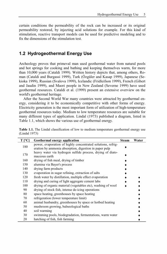
many different types of application. Lindal (1973) published a diagram, listed in
Table 1.1, which shows the various use of geothermal energy.
Table 1.1. The Lindal classification of low to medium temperature geothermal energy use
(Lindal 1973)
T [°C] Geothermal energy application Steam Water
180power, evaporation of highly concentrated solutions, refrig-
eration by ammonia absorption, digestion in paper pulp ♦
170heavy water via hydrogen sulfide process, drying of diato-
maceous earth ♦
160 drying of fish meal, drying of timber ♦150 alumina via Bayer's process ♦140 drying farm products ♦130 evaporation in sugar refining, extraction of salts ♦120 fresh water by distillation, multiple effect evaporation ♦ ♦110 drying and curing of light aggregate cement labs ♦ ♦100 drying of organic material (vegetables etc), washing of wool ♦ ♦90 drying of stock fish, intense de-icing operations ♦80 space heating, greenhouses by space heating ♦70 refrigeration (lower temperature limit) ♦60 animal husbandry, greenhouses by space or hotbed heating ♦50 mushroom growing, balneological baths ♦40 soil warming ♦30 swimming pools, biodegradation, fermentations, warm water ♦20 hatching of fish, fish farming ♦
6 General Significance of Geochemical Models of Hydrothermal Systems
Most geothermal resources can be used for space heating applications (e.g. ur-
ban district heating, fish farming, and greenhouse heating). Only the hotter sys-
tems (>180°C) are used to generate electricity through the production of steam.
Commercial extraction of heat from active hydrothermal systems has been grow-
ing steadily over the past few decades. Nevertheless, extraction of minerals from
fossil hydrothermal systems continues to have a much larger economic signifi-
cance and provides a major practical impetus for research on hydrothermal sys-
tems.
Huttrer (2000) assessed the status of international geothermal power generation
from all nations generating or planning to generate electricity and revealed that:
(1) geothermally fueled electric power is being generated in 21 nations, (2) the in-
stalled capacity has reached 7,974 MWelectric which is a 16.7% increase since 1995,
(3) the total energy generated is at least 49,261 GWh, and (4) during the last five
years, about 1,165 wells more than 100 meters deep were drilled. Huttrer (2000)
concluded that greater increases in the total international installed geothermal gen-
eration capacity were inhibited by the economic crisis that occurred in Southeast
Asia and by the low petroleum prices prevailing within the last decade.
The recent worldwide application of geothermal heat for direct utilization is re-
viewed for 60 countries by Lund and Freeston (2000), of which 55 reported some
form of geothermal direct utilization. An estimate of the installed thermal power at
the end of 1999 (1995 in brackets) from the current reports is 16,209 MWthermal
[8,660 MWthermal] utilizing at least 64,416 kg s-1
[37,050 kg s-1
] of fluid, and the
thermal energy used is 162,009 TJ yr-1
[112,441 TJ yr-1
]. The distribution of the
thermal energy used by category is approximately 37% for space heating, 22% for
bathing and swimming pool heating, 14% for geothermal heat pumps, 12% for
greenhouse heating, 7% for aquaculture pond and raceway heating, 6% for indus-
trial applications, less than 1% each for agricultural drying, snow melting, air con-
ditioning and other uses. The reported data for number of wells drilled was 1,028
over the five years. Research progress manifests by a total of 841 chemical inter-
pretations of geothermal fields (Freeston 1995, Lund and Freeston 2000).
Schellschmidt et al. (2000) pointed out that by the end of 1999 direct thermal
use of geothermal energy in Germany amounted to an installed thermal power of
roughly 397 MWthermal. Of this sum, approximately 55 MWthermal are generated in
27 major centralized installations. Small, decentralized earth-coupled heat pumps
and groundwater heat pumps are estimated to contribute an additional 342
MWthermal. By the year 2002 an increase in total installed power of about 120
MWthermal is expected: 82 MWthermal from major central and 40 MWthermal from
small, decentralized installations. This would boost direct thermal use in Germany
close to an installed thermal power of 517 MWthermal. At present no electric power
is produced from geothermal resources in Germany, whose annual final energy
consumption at present amounts to about 9469 PJ. It is less than the corresponding
primary energy because of losses, mainly due to conversion and distribution. This
is equivalent to a total consumed power of approximately 300,000 MW per year.
Almost 60 % of this energy is required as heat. The total technical potential for the
direct use of geothermal energy in Germany is 2125 PJ a-1
, with a weighting ac-
cording to the local variation in the demand for heat; equivalent to a maximum
Reservoir Exploration and Management 7
thermal power generation of about 67,380 MWthermal. That corresponds to about
22 % of the country’s annual final energy consumption, or roughly 37 % of its
demand for heat. However, at present only about 6 ‰ of the existing maximum
technical potential for direct thermal use of geothermal energy meets the demand
for heat. If the vast potential of geothermal energy for direct thermal use was util-
ized to substitute fossil fuels, roughly 100 million tons less of CO2 would be re-
leased to the atmosphere annually, equivalent to about 10 % of Germany’s CO2
output in 1998.
1.3 Reservoir Exploration and Management
Before drawing up a geothermal exploration program, geophysical surveys are
done. The advantage of geophysical data collection from deep geological forma-
tions is the fact that they are indirectly obtained from the surface or from depth
close to the surface. In the 1920s it was shown for the first time, that for example,
electrical resistivity measurements could be made in a well and that the readings
were different for different geological layers (Hearst et al. 2000). Due to more and
more sophisticated measurements, the discovery and location of reservoirs is done
with the help of these subsurface methods. These measurements use electromag-
netic fields and waves, acoustic waves, neutron scattering, gamma-ray radiation,
nuclear magnetic resonance, infrared spectroscopy, and pressure and temperature
sensors, with the aim to characterize in detail the geological structure within the
vicinity of a bore. However, there is no single technique adequate to define the
structure and properties of a whole reservoir. This is a fact which led to significant
efforts and advances in predictive reservoir simulation within the last two decades.
During the 1960s, when our environment was in a healthier state than it is at
present and we were less aware of the threat to the earth, geothermal energy was
still considered a "clean energy". There is actually no way of producing or trans-
forming energy into a form that can be utilized by humanity without direct or indi-
rect impact on the environment. Similarly, exploitation of geothermal energy also
has an impact on the environment, although it must be said that it is one of the
least polluting. Models should be used to ensure exploitation of geothermal re-
sources to be as harmless as possible, because any modification to our environ-
ment must be evaluated carefully, in deference to the relevant laws and regula-
tions. The danger is that an apparently insignificant modification could trigger a
chain of events whose impact is difficult to fully assess beforehand. In most cases
the degree to which geothermal exploitation affects the environment is propor-
tional to the scale of such exploitation (Lunis and Breckenridge 1991).
The use of computer modeling in the planning and management of the devel-
opment of geothermal fields has become standard practice during the last 10 – 15
years. The computer power available in the 1980s limited the size of the computa-
tional meshes used and many of them were based on geometrically simple models.
In addition to modeling specific geothermal fields, an important application of
numerical reservoir simulation has been in the study of generic issues of geother-
8 General Significance of Geochemical Models of Hydrothermal Systems
mal reservoir dynamics, and fluid and heat processes. It is also possible to predict
the response of recent geothermal systems to various natural and industrial proc-
esses. This is important for reservoir management and sustainable exploitation of
the resources (O'Sullivan 2001).
Geochemical data are necessary for delineating favorable exploration areas, es-
timating the recoverable geothermal resources from a given reservoir, and identi-
fying potential pollution, waste disposal, and corrosion problems. The objectives
are to study the chemistry and controls on the chemistry of water in geothermal
and other subsurface systems to provide basic data needed (Pham et al. 2001).
1.4 Geochemical Models
Economic and sustainable exploitation of geothermal reservoirs requires powerful
reactive transport models. The models must cover two aspects: geochemical and
hydrodynamic processes. Geochemical processes include, among others, aqueous
speciation and redox reactions, interface reactions, precipitation / dissolution of
minerals and colloids. Hydrodynamic transport processes mainly include diffusion
and migration due to advective forces, leading to dispersion of the chemical spe-
cies in space and time. Modern development is to consider geochemical and hy-
drodynamic transport processes interdependently, because geochemistry and
hydrogeology are closely entangled.
Geochemist's goal is to describe the chemical states of natural waters, including
how dissolved mass is distributed among aqueous species, and to understand how
such waters will react with minerals, gases, and fluids of the Earth’s crust and hy-
drosphere. This can be done involving simple chemical systems in which the reac-
tions can be anticipated through experience and evaluated by hand calculation.
Facing more complex problems, one must rely increasingly on quantitative models
of solution chemistry to find answers.
Geochemists now use quantitative models in order to understand sediment
diagenesis and hydrothermal alteration, to explore for ore deposits, to determine
which contaminants will migrate from mine tailings and toxic waste sites, to pre-
dict scaling in geothermal wells and the outcome of steam-flooded oil reservoirs,
to solve kinetic rate equations, to manage injection wells, to evaluate laboratory
experiments, and to study acid rain, among many examples. The advantage is that
geochemical models allow geoscientists to estimate the results of a hydrothermal
experiment or to interpret reservoirs spending less amounts of time and money.
The field of reactive transport within the Earth Sciences has become a highly
multidisciplinary area of research. The field encompasses a number of diverse dis-
ciplines including geochemistry, geology, physics, chemistry, hydrology, and en-
gineering. A wide variety of geochemical processes including such diverse phe-
nomena as the transport of radiogenic and toxic waste products, diagenesis,
hydrothermal ore deposit formation, and metamorphism are the result of reactive
transport in the subsurface. Such systems can be viewed as open reactors where
chemical change is driven by the interaction between migrating fluids and solid
Geochemical Models 9
phases. The evolution of these systems involves diverse processes including fluid
flow, heat transfer, solute transport, and chemical reactions, each with different
characteristic time scales. The ability to quantify reactive transport in natural sys-
tems has advanced dramatically over the past decades. Much of this progress is
due to the exponential increase in computational power. Taking advantage of this
increase, numerous comprehensive reactive transport models have been developed
and applied to natural phenomena. These models can be used either qualitatively
or quantitatively to provide insight into natural processes. Quantitative models
force the investigator to evaluate or falsify ideas by putting real numbers into an
often-vague hypothesis. As a consequence, a thinking process is initiated along a
path that may result in acceptance, rejection, or modification of the original hy-
pothesis. Used qualitatively, models provide insight into general features of a par-
ticular phenomenon, rather than specific details.
One of the major questions facing the use of hydrogeochemical models is
whether or not they can be used with confidence explaining history as well as pre-
dicting future evolution of natural groundwater or geothermal systems. There is
much controversy concerning the validity and uncertainties of non-reactive fluid
flow models (Konikow and Bredehoeft 1992). Adding chemical interaction to
these flow models only confounds the problem. Although such models may accu-
rately integrate the governing physical and chemical equations, many uncertainties
are inbuilt in characterizing the natural system itself. These systems are inherently
heterogeneous on a variety of scales rendering it highly challenging to know pre-
cisely the many details of the flow system and chemical composition of the fluids
and host rocks. Other properties of natural systems such as permeability and min-
eral surface area, to name just two, may have to be approximated with little preci-
sion. Because of these uncertainties, it is important to delineate to what extent a
certain numerical reactive transport model is useful in making accurate quantita-
tive predictions. Nevertheless, reactive transport models should allow for predict-
ing the outcome for the particular representation of the porous medium used in the
model.
Heat in Earth's crust represents the greatest potential contribution to the world's
energy base. Yet this important energy source is at present markedly underuti-
lized. The principal reasons for this situation are the high costs currently associ-
ated with geothermal energy production and exploration and the lack of technol-
ogy to reduce these costs. Many of the significant problems encountered by the
geothermal industry reflect complicated chemical interactions between solids,
gases and liquids. Adverse chemical effects, such as scale formation, corrosion
and noxious gas emission, which can arise from the manipulation of the high tem-
perature natural fluids driving the energy production process, are expensive to
control. Mineral precipitation for example, can not only damage plant equipment
and wells but also significantly decrease the permeability of the formations con-
taining the geothermal fluids, thereby limiting the longevity of the resource itself.
The ability to predict these chemical behaviors and the heat content of a reservoir
as well as to design optimal operating strategies would significantly increase the
cost effectiveness of geothermal energy production. Predicting potential chemical
problems will become even more important as deeper, higher temperature geo-
10 General Significance of Geochemical Models of Hydrothermal Systems
thermal systems with very high development costs, will be utilized to meet future
energy needs (Moeller et al. 2000).
In order to understand the chemical processes in fossil or recent geothermal
systems or to predict the chemistry during geothermal energy production, it is nec-
essary to understand the thermodynamics and kinetics of the waters within the
hosting rock formation or the production processes. Unfortunately, the chemical
behavior of these waters, which are often high temperature brines, is a very com-
plex function of their composition, temperature and pressure. Since these variables
can change significantly during lifetime of the geothermal reservoir or resource,
the past experience of geothermal energy production therefore may not be a reli-
able guide for future performance. Laboratory simulations are costly and limited
to the experimental conditions selected. Reactive transport simulation is a testing
strategy to control unwanted behavior in active operations as well as to forecast
the value of geothermal reservoirs as potential production sites and last but not
least to evaluate geothermal system history.
Finally, it should be mentioned that the numerical solution of the geochemical
model equations often is the only recourse to analyze a hydrothermal system
where investigations must be carried out over geologic time spans. Without such
models it would be impossible to analyze fossil hydrothermal systems, because
performing laboratory experiments would take too much time and recently active
geothermal systems are most often within a different stage of development.
2 Concepts, Classification, and Chemistry of
Geothermal Systems
Main concepts and a classification of different types of geothermal systems are
presented in this chapter. Particular attention is given to chemical, physical, and
geometric features of the geothermal systems inferred from active geothermal ar-
eas or reconstructed from geological observations.
Additionally, different types of water existing in geothermal reservoirs world-
wide are reviewed here. They are discussed and related to the basic processes that
dominate their chemistry. The chemistry of geothermal waters discharged from
wells provides specific information about the deep fluids in geothermal systems
and how they relate to natural discharges from springs at Earth’s surface. This
knowledge can be used to obtain essential information about reservoir behavior
before and during exploitation and to set up conceptual models of reservoirs.
Derivation of the hydrologic and chemical structure of geothermal systems forms
the basis for reactive transport simulation, here and in general.
2.1 Conceptual Model and Classification
Geothermal systems as hosts of resources or potential reservoirs are also called
geothermal fields. They are found throughout the world in regions with normal or
above normal geothermal gradients, and especially in regions around tectonic
plate margins where the geothermal gradient may be significantly higher than the
average value. Geothermal systems are encountered in a range of geological set-
tings, and are increasingly developed as an energy source. They can be described
schematically as the distribution of waters circulating laterally and vertically at
various temperatures and pressures in the upper crust of the Earth. The geothermal
system transfers heat from a heat source to a heat sink, usually the free surface
(Hochstein 1990). A geothermal system is made up of three main elements: a heat
source, a reservoir and a fluid, which is the carrier that transfers the heat. The res-
ervoir is a volume of permeable rocks from which the circulating fluids extract the
heat. The geothermal fluid is water, in the majority of cases meteoric water (rain,
lake, river), in the liquid or vapor phase, depending on its temperature and pres-
sure (Fig. 2.1). Geothermal fluids often discharge at the surface. Hydrothermal
mineral deposits are formed due to circulation of the warm to hot fluids (about 50
to > 500°C) that leach, transport and subsequently precipitate their mineral load
usually to the discharge site of the system (e.g. single conduit, fracture network).
Michael Kuhn: LNES 103, pp. 11–46, 2004.c© Springer-Verlag Berlin Heidelberg 2004
12 Concepts, Classification, and Chemistry of Geothermal Systems
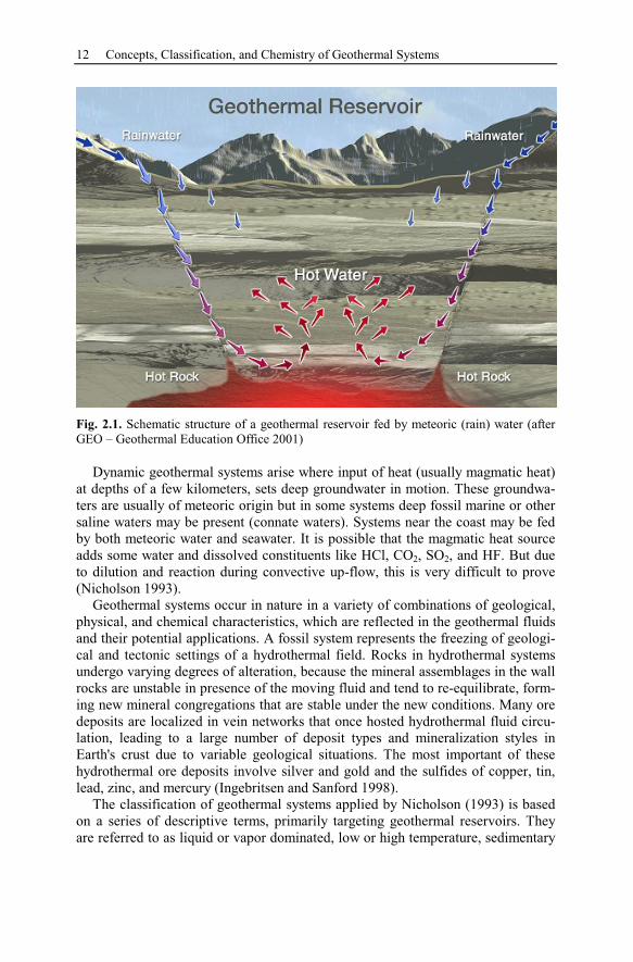
Fig. 2.1. Schematic structure of a geothermal reservoir fed by meteoric (rain) water (after
GEO – Geothermal Education Office 2001)
Dynamic geothermal systems arise where input of heat (usually magmatic heat)
at depths of a few kilometers, sets deep groundwater in motion. These groundwa-
ters are usually of meteoric origin but in some systems deep fossil marine or other
saline waters may be present (connate waters). Systems near the coast may be fed
by both meteoric water and seawater. It is possible that the magmatic heat source
adds some water and dissolved constituents like HCl, CO2, SO2, and HF. But due
to dilution and reaction during convective up-flow, this is very difficult to prove
(Nicholson 1993).
Geothermal systems occur in nature in a variety of combinations of geological,
physical, and chemical characteristics, which are reflected in the geothermal fluids
and their potential applications. A fossil system represents the freezing of geologi-
cal and tectonic settings of a hydrothermal field. Rocks in hydrothermal systems
undergo varying degrees of alteration, because the mineral assemblages in the wall
rocks are unstable in presence of the moving fluid and tend to re-equilibrate, form-
ing new mineral congregations that are stable under the new conditions. Many ore
deposits are localized in vein networks that once hosted hydrothermal fluid circu-
lation, leading to a large number of deposit types and mineralization styles in
Earth's crust due to variable geological situations. The most important of these
hydrothermal ore deposits involve silver and gold and the sulfides of copper, tin,
lead, zinc, and mercury (Ingebritsen and Sanford 1998).
The classification of geothermal systems applied by Nicholson (1993) is based
on a series of descriptive terms, primarily targeting geothermal reservoirs. They
are referred to as liquid or vapor dominated, low or high temperature, sedimentary
Conceptual Model and Classification 13
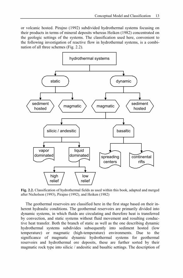
or volcanic hosted. Pirajno (1992) subdivided hydrothermal systems focusing on
their products in terms of mineral deposits whereas Heiken (1982) concentrated on
the geologic settings of the systems. The classification used here, convenient to
the following investigation of reactive flow in hydrothermal systems, is a combi-
nation of all three schemes (Fig. 2.2).
hydrothermal systems
static dynamic
sediment
hostedmagmatic
sediment
hostedmagmatic
silicic / andesitic basaltic
vapor
dominated
liquid
dominated
high
relief
low
relief
spreading
centers
continental
rifts
Fig. 2.2. Classification of hydrothermal fields as used within this book, adapted and merged
after Nicholson (1993), Pirajno (1992), and Heiken (1982)
The geothermal reservoirs are classified here in the first stage based on their in-
herent hydraulic conditions. The geothermal reservoirs are primarily divided into
dynamic systems, in which fluids are circulating and therefore heat is transferred
by convection, and static systems without fluid movement and resulting conduc-
tive heat transfer. Both the branch of static as well as the one describing dynamic
hydrothermal systems subdivides subsequently into sediment hosted (low
temperature) or magmatic (high-temperature) environments. Due to the
significance of magmatic dynamic hydrothermal systems for geothermal
reservoirs and hydrothermal ore deposits, these are further sorted by their
magmatic rock type into silicic / andesitic and basaltic settings. The description of
14 Concepts, Classification, and Chemistry of Geothermal Systems
silicic / andesitic and basaltic settings. The description of the basaltic systems dis-
tributes into mid-ocean ridge spreading centers and continental rift settings. The
silicic / andesitic hydrothermal environments are divided into vapor and liquid
dominated systems and the latter additionally into low or high relief settings.
2.2 Static – Conductive Systems
The mean conductive heat flow measured near Earth’s surface is approximately
70 mW m-2
(e.g. Chapman and Pollack 1975). Correcting for the effects of hydro-
thermal circulation in the oceanic crust brings the mean global heat flux to
87 mW m-2
(Pollack et al. 1993). Integrated over the surface of the globe, this
amounts to a heat loss of more than 4x10¹³
W. The main source of heat in the crust
(shallow heat source) is the continually radioactive decay of long-lived isotopes of
uranium (238
U,235
U), thorium (232
Th), and potassium (40
K). However, Earth's main
deep heat source is the heat of primordial energy of planetary accretion (Lubimova
1968).
2.2.1 Magmatic Systems
Static, magmatic systems are usually related to shallow or deep-seated granitic
plutonism generated by H2O-rich magmas (> 8 wt.%). These magmas crystallize
at depths between a few kilometers to over 10 km but normally do not vent at the
surface (Pirajno 1992).
Hydrothermal fluids of such a system are assumed to be generated entirely
within the cooling magma body and set up a closed system. This situation results
in hydrogen-ion metasomatism (see below) leading to so-called greisen-related
deposits. The term greisen refers to an assemblage of quartz and muscovite ac-
companied by varying amounts of minerals like fluorite, topaz, tourmaline and
other F- or B-rich minerals (Burt 1981). Greisen systems are normally associated
with Sn, W, Mo, Be, Bi and Li mineralization.
2.2.2 Sediment Hosted Systems
Static systems are characteristically found in strata deposited in deep sedimentary
basins. The fluids are derived from the formation waters trapped within the thick
sedimentary sequences. These waters attain reservoir temperatures of around 70-
150°C at depths of 2-4 km, due to conductive heat flow. Geothermal fields in
sediment hosted systems are normally called low-temperature because they are of-
ten only suitable for direct energy use and not for power production. The fluids are
typically very saline chloride waters or brines, which remain trapped, as the verti-
cal permeability is low within the formations, until released tectonically or by
Dynamic – Convective Systems 15
drilling. Examples of such fields are located in North and Eastern Europe, Russia,
and Australia.
The following chapters will deal to a great extent with these static systems and
additionally with low temperature dynamic systems (see below). Both are of
greatest importance for Europe. Especially in Germany, static low temperature
systems are the only ones currently under exploitation.
2.3 Dynamic – Convective Systems
Magmatic intrusions, leading to convective heat transfer by geothermal water cir-
culation, are the source of thermal energy to most of Earth’s high temperature
(> 150°C) hydrothermal systems. However, a few high-temperature systems occur
in areas of little or no apparent volcanic activity. These particular systems appear
to be caused by deep circulation of meteoric water, leading to convective heat
transfer, in areas of above-average conductive heat flow (e.g. Beowawe, Nevada,
published by White 1992).
2.3.1 Magmatic - High-Temperature
In geological settings with magmatic or high-temperature systems the geothermal
gradient is several times above the crustal average and rock temperatures of sev-
eral hundred degrees Celsius exist at depths of only a few kilometers. The loca-
tions of these geothermal fields is invariably tectonically determined, and they are
often found in areas of block faulting, grabens or rifting and in collapsed caldera
structures, with reservoir depths of around 1-3 km. Typical settings are around ac-
tive plate margins (Fig. 2.3) such as subduction zones (e.g. Pacific Rim), spread-
ing ridges (Mid-Atlantic), rift zones (East Africa) and within orogenic belts
(Mediterranean, Himalaya).
High-temperature systems are often volcanogenic, with the heat provided by in-
trusive masses. Geothermal systems also develop on the flanks of young volca-
noes. As mentioned, high-temperature fields with a non-volcanogenic or tectonic
heat source are less common (Nicholson 1993).
Hydrothermal systems related to volcano-plutonic and volcanic settings start as
static-magmatic systems (described above), in the closed system of a plutonic
body. The magmatic body rises closer to the surface or even ruptures it forming a
stratovolcano. Due to the igneous bodies, providing a powerful heat engine, con-
vection cells form with fluids supplied from meteoric waters. This environment is
typical for porphyry or epithermal ore deposits and alteration features known as
potassic, propylitic, phyllic, and argillic (all described below). The active time
span of such systems may range from 105 to 10
6 years (Henley and Ellis 1983).
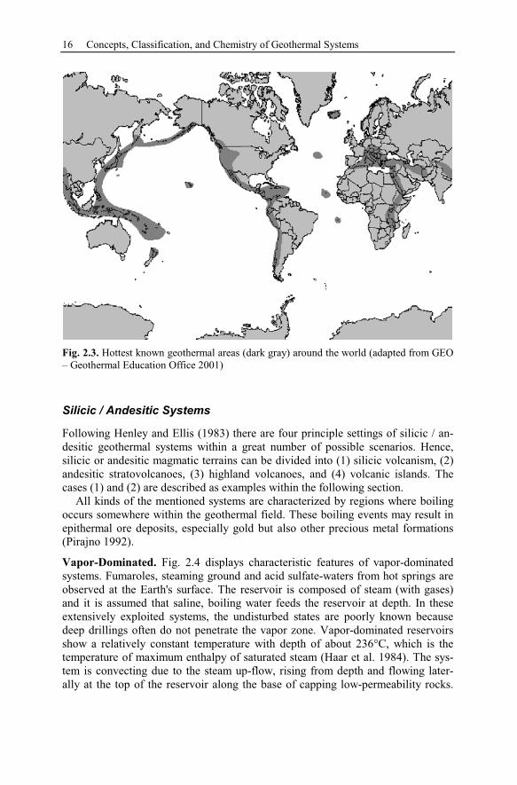
16 Concepts, Classification, and Chemistry of Geothermal Systems
Fig. 2.3. Hottest known geothermal areas (dark gray) around the world (adapted from GEO
– Geothermal Education Office 2001)
Silicic / Andesitic Systems
Following Henley and Ellis (1983) there are four principle settings of silicic / an-
desitic geothermal systems within a great number of possible scenarios. Hence,
silicic or andesitic magmatic terrains can be divided into (1) silicic volcanism, (2)
andesitic stratovolcanoes, (3) highland volcanoes, and (4) volcanic islands. The
cases (1) and (2) are described as examples within the following section.
All kinds of the mentioned systems are characterized by regions where boiling
occurs somewhere within the geothermal field. These boiling events may result in
epithermal ore deposits, especially gold but also other precious metal formations
(Pirajno 1992).
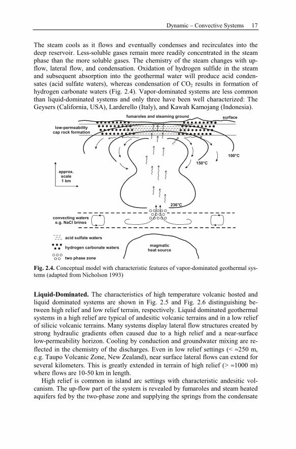
Vapor-Dominated. Fig. 2.4 displays characteristic features of vapor-dominated
systems. Fumaroles, steaming ground and acid sulfate-waters from hot springs are
observed at the Earth's surface. The reservoir is composed of steam (with gases)
and it is assumed that saline, boiling water feeds the reservoir at depth. In these
extensively exploited systems, the undisturbed states are poorly known because
deep drillings often do not penetrate the vapor zone. Vapor-dominated reservoirs
show a relatively constant temperature with depth of about 236°C, which is the
temperature of maximum enthalpy of saturated steam (Haar et al. 1984). The sys-
tem is convecting due to the steam up-flow, rising from depth and flowing later-
ally at the top of the reservoir along the base of capping low-permeability rocks.
Dynamic – Convective Systems 17
The steam cools as it flows and eventually condenses and recirculates into the
deep reservoir. Less-soluble gases remain more readily concentrated in the steam
phase than the more soluble gases. The chemistry of the steam changes with up-
flow, lateral flow, and condensation. Oxidation of hydrogen sulfide in the steam
and subsequent absorption into the geothermal water will produce acid conden-
sates (acid sulfate waters), whereas condensation of CO2 results in formation of
hydrogen carbonate waters (Fig. 2.4). Vapor-dominated systems are less common
than liquid-dominated systems and only three have been well characterized: The
Geysers (California, USA), Larderello (Italy), and Kawah Kamojang (Indonesia).
acid sulfate waters
hydrogen carbonate waters
two phase zone
magmatic
heat source
fumaroles and steaming ground
convecting waters
e.g. NaCl brines
236°C
low-permeability
cap rock formation
150°C
100°C
approx.
scale
1 km
surface
Fig. 2.4. Conceptual model with characteristic features of vapor-dominated geothermal sys-
tems (adapted from Nicholson 1993)
Liquid-Dominated. The characteristics of high temperature volcanic hosted and
liquid dominated systems are shown in Fig. 2.5 and Fig. 2.6 distinguishing be-
tween high relief and low relief terrain, respectively. Liquid dominated geothermal
systems in a high relief are typical of andesitic volcanic terrains and in a low relief
of silicic volcanic terrains. Many systems display lateral flow structures created by
strong hydraulic gradients often caused due to a high relief and a near-surface
low-permeability horizon. Cooling by conduction and groundwater mixing are re-
flected in the chemistry of the discharges. Even in low relief settings (< ≈250 m,
e.g. Taupo Volcanic Zone, New Zealand), near surface lateral flows can extend for
several kilometers. This is greatly extended in terrain of high relief (> ≈1000 m)
where flows are 10-50 km in length.
High relief is common in island arc settings with characteristic andesitic vol-
canism. The up-flow part of the system is revealed by fumaroles and steam heated
aquifers fed by the two-phase zone and supplying the springs from the condensate
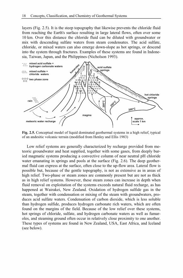
18 Concepts, Classification, and Chemistry of Geothermal Systems
layers (Fig. 2.5). It is the steep topography that likewise prevents the chloride fluid
from reaching the Earth's surface resulting in large lateral flows, often over some
10 km. Over this distance the chloride fluid can be diluted with groundwater or
mix with descending sulfate waters from steam condensates. The acid sulfate,
chloride, or mixed waters can also emerge down-slope as hot springs, or descend
into the system through fractures. Examples of these systems are found in Indone-
sia, Taiwan, Japan, and the Philippines (Nicholson 1993).
mixed acid sulfate +
hydrogen carbonate waters
mixed sulfate +
chloride waters
two phase zone
rain
fum
aro
les
meteoric water recharge
magma
acid sulfate
springs
hot chloride
springs
approx.
scale 1 km
200°C
250°C
30
0°C
Fig. 2.5. Conceptual model of liquid dominated geothermal systems in a high relief, typical
of an andesitic volcanic terrain (modified from Henley and Ellis 1983)
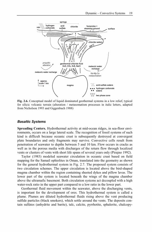
Low relief systems are generally characterized by recharge provided from me-
teoric groundwater and heat supplied, together with some gases, from deeply bur-
ied magmatic systems producing a convective column of near neutral pH chloride
water emanating in springs and pools at the surface (Fig. 2.6). The deep geother-
mal fluid can express at the surface, often close to the up-flow area. Lateral flow is
possible but, because of the gentle topography, is not as extensive as in areas of
high relief. Two-phase or steam zones are commonly present but are not as thick
as in high relief systems. However, these steam zones can increase in depth when
fluid removal on exploitation of the systems exceeds natural fluid recharge, as has
happened at Wairakei, New Zealand. Oxidation of hydrogen sulfide gas in the
steam, together with condensation or mixing of the steam with groundwaters, pro-
duces acid sulfate waters. Condensation of carbon dioxide, which is less soluble
than hydrogen sulfide, produces hydrogen carbonate rich waters, which are often
found on the margins of the field. Because of the low relief over these systems,
hot springs of chloride, sulfate, and hydrogen carbonate waters as well as fumar-
oles, and steaming ground often occur in relatively close proximity to one another.
These types of systems are found in New Zealand, USA, East Africa, and Iceland
(see below).
Dynamic – Convective Systems 19
rain
meteoric water recharge
meteoric water
recharge
acid sulfate waters
hydrogen carbonate
waters
two phase zone
magma
chloride waters
fumaroles +
steaming ground chloride
approx.
scale 1 km
hydrogen
carbonate
acid
sulfate
springs
propylitic
alteration
Na-Mg-Ca
metasomatism
arg
illic
altera
tion
Hm
eta
so
ma
tism
phyl
licalte
ratio
n
H-K
me
tas.
200°C
250°C
30
0°C
400°C
surface
Fig. 2.6. Conceptual model of liquid dominated geothermal systems in a low relief, typical
for silicic volcanic terrain (alteration / metasomatism processes in italic letters, adapted
from Nicholson 1993 and Giggenbach 1988)
Basaltic Systems
Spreading Centers. Hydrothermal activity at mid-ocean ridges, in sea-floor envi-
ronments, occurs on a large lateral scale. The recognition of fossil systems of such
kind is difficult because oceanic crust is subsequently destroyed at convergent
plate boundaries and only fragments may survive. Convective cells result from
penetration of seawater to depths between 5 and 10 km. Flow occurs in cracks as
well as in the porous media with discharges of the return flow through localized
vents or clusters of vents with short life spans of several years only (Pirajno 1992).
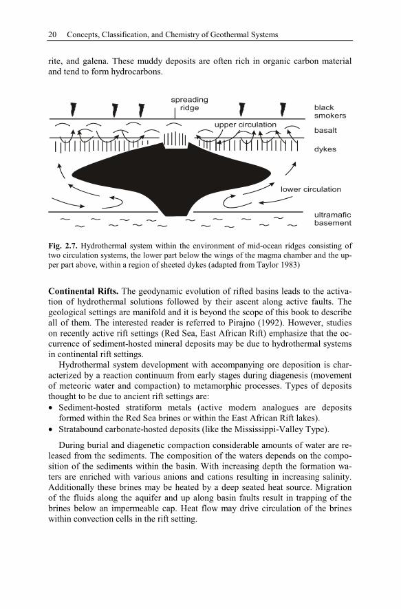
Taylor (1983) modeled seawater circulation in oceanic crust based on field
mapping for the Samail ophiolites in Oman, translated into the geometry as shown
for the general hydrothermal system in Fig. 2.7. The proposed system consists of
two circulation schemes. The upper circulation is located above the bird-shaped
magma chamber within the region containing sheeted dykes and pillow lavas. The
lower part of the system is located beneath the wings of the magma chamber
above the ultramafic basement. Both circulation systems act decoupled with a high
water-rock ratio in the upper part compared to a low ratio in the lower part.
Geothermal fluid movement within the seawater, above the discharging vents,
is important for the development of ores. This hydrothermal system is called a
plume. Plumes are diluted hydrothermal fluids rising above the vent producing
sulfide particles (black smokers), which settle around the vents. The deposits con-
tain sulfates (anhydrite and barite), talc, calcite, pyrrhotite, sphalerite, chalcopy-
20 Concepts, Classification, and Chemistry of Geothermal Systems
rite, and galena. These muddy deposits are often rich in organic carbon material
and tend to form hydrocarbons.
basalt
dykes
ultramafic
basement
black
smokers
lower circulation
upper circulation
Fig. 2.7. Hydrothermal system within the environment of mid-ocean ridges consisting of
two circulation systems, the lower part below the wings of the magma chamber and the up-
per part above, within a region of sheeted dykes (adapted from Taylor 1983)
Continental Rifts. The geodynamic evolution of rifted basins leads to the activa-
tion of hydrothermal solutions followed by their ascent along active faults. The
geological settings are manifold and it is beyond the scope of this book to describe
all of them. The interested reader is referred to Pirajno (1992). However, studies
on recently active rift settings (Red Sea, East African Rift) emphasize that the oc-
currence of sediment-hosted mineral deposits may be due to hydrothermal systems
in continental rift settings.
Hydrothermal system development with accompanying ore deposition is char-
acterized by a reaction continuum from early stages during diagenesis (movement
of meteoric water and compaction) to metamorphic processes. Types of deposits
thought to be due to ancient rift settings are:
• Sediment-hosted stratiform metals (active modern analogues are deposits
formed within the Red Sea brines or within the East African Rift lakes).
• Stratabound carbonate-hosted deposits (like the Mississippi-Valley Type).
During burial and diagenetic compaction considerable amounts of water are re-
leased from the sediments. The composition of the waters depends on the compo-
sition of the sediments within the basin. With increasing depth the formation wa-
ters are enriched with various anions and cations resulting in increasing salinity.
Additionally these brines may be heated by a deep seated heat source. Migration
of the fluids along the aquifer and up along basin faults result in trapping of the
brines below an impermeable cap. Heat flow may drive circulation of the brines
within convection cells in the rift setting.
Dynamic – Convective Systems 21
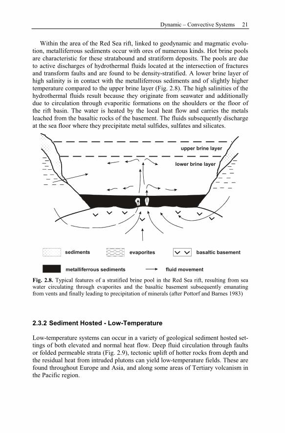
Within the area of the Red Sea rift, linked to geodynamic and magmatic evolu-
tion, metalliferrous sediments occur with ores of numerous kinds. Hot brine pools
are characteristic for these stratabound and stratiform deposits. The pools are due
to active discharges of hydrothermal fluids located at the intersection of fractures
and transform faults and are found to be density-stratified. A lower brine layer of
high salinity is in contact with the metalliferrous sediments and of slightly higher
temperature compared to the upper brine layer (Fig. 2.8). The high salinities of the
hydrothermal fluids result because they originate from seawater and additionally
due to circulation through evaporitic formations on the shoulders or the floor of
the rift basin. The water is heated by the local heat flow and carries the metals
leached from the basaltic rocks of the basement. The fluids subsequently discharge
at the sea floor where they precipitate metal sulfides, sulfates and silicates.
upper brine layer
lower brine layer
sediments basaltic basement
fluid movementmetalliferrous sediments
Fig. 2.8. Typical features of a stratified brine pool in the Red Sea rift, resulting from sea
water circulating through evaporites and the basaltic basement subsequently emanating
from vents and finally leading to precipitation of minerals (after Pottorf and Barnes 1983)
2.3.2 Sediment Hosted - Low-Temperature
Low-temperature systems can occur in a variety of geological sediment hosted set-
tings of both elevated and normal heat flow. Deep fluid circulation through faults
or folded permeable strata (Fig. 2.9), tectonic uplift of hotter rocks from depth and
the residual heat from intruded plutons can yield low-temperature fields. These are
found throughout Europe and Asia, and along some areas of Tertiary volcanism in
the Pacific region.
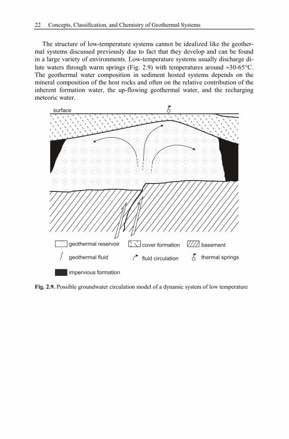
22 Concepts, Classification, and Chemistry of Geothermal Systems
The structure of low-temperature systems cannot be idealized like the geother-
mal systems discussed previously due to fact that they develop and can be found
in a large variety of environments. Low-temperature systems usually discharge di-
lute waters through warm springs (Fig. 2.9) with temperatures around ≈30-65°C.
The geothermal water composition in sediment hosted systems depends on the
mineral composition of the host rocks and often on the relative contribution of the
inherent formation water, the up-flowing geothermal water, and the recharging
meteoric water.
geothermal reservoir cover formation basement
geothermal fluid fluid circulation thermal springs
impervious formation
surface
Fig. 2.9. Possible groundwater circulation model of a dynamic system of low temperature
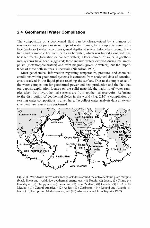
Geothermal Water Compilation 23
2.4 Geothermal Water Compilation
The composition of a geothermal fluid can be characterized by a number of
sources either as a pure or mixed type of water. It may, for example, represent sur-
face (meteoric) water, which has gained depths of several kilometers through frac-
tures and permeable horizons, or it can be water, which was buried along with the
host sediments (formation or connate waters). Other sources of water in geother-
mal systems have been suggested; these include waters evolved during metamor-
phism (metamorphic waters) and from magmas (juvenile waters), but the impor-
tance of these both sources is uncertain (Nicholson 1993).
Most geochemical information regarding temperature, pressure, and chemical
conditions within geothermal systems is extracted from analytical data of constitu-
ents dissolved in the liquid phase reaching the surface. Due to the importance of
the water composition for geothermal power and heat production and the fact that
ore deposit exploration focuses on the solid material, the majority of water sam-
ples taken from hydrothermal systems are from geothermal reservoirs. Referring
to the distribution of geothermal fields in the world (Fig. 2.10) a compilation of
existing water compositions is given here. To collect water analysis data an exten-
sive literature review was performed.
Fig. 2.10. Worldwide active volcanoes (black dots) around the active tectonic plate margins
(black lines) and worldwide geothermal energy use; (1) Russia, (2) Japan, (3) China, (4)
Himalayan, (5) Philippines, (6) Indonesia, (7) New Zealand, (8) Canada, (9) USA, (10)
Mexico, (11) Central America, (12) Andes, (13) Caribbean, (14) Iceland and Atlantic is-
lands, (15) Europe and Mediterranean, and (16) Africa (adapted from Topinka 1997)
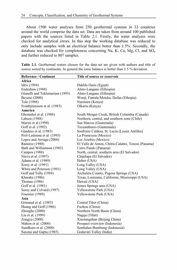
24 Concepts, Classification, and Chemistry of Geothermal Systems
About 1500 water analyses from 250 geothermal systems in 33 countries
around the world comprise the data set. Data are taken from around 100 published
papers with the sources listed in Table 2.1. Firstly, the water analyses were
checked for analytical errors. In this step the working database was reduced to
only include samples with an electrical balance better than ± 5%. Secondly, the
database was checked for completeness concerning Na, K, Ca, Mg, Cl, and SO4
and further reduced to 807 samples.
Table 2.1. Geothermal waters chosen for the data set are given with authors and title of
source sorted by continents. In general the ionic balance is better than ± 5 % deviation
Reference / Continent Title of source or reservoir
Africa
Idris (1994) Dakhla Oasis (Egypt)
Endeshaw (1988) Aluto-Langano (Ethiopia)
Gianelli and Teklemariam (1993) Aluto-Langano (Ethiopia)
Beyene (2000) Wonji, Fantale/Meteka, Dofan (Ethopia)
Tole (1988) Narosura (Kenya)
Svanbjörnsson et al. (1983) Olkaria (Kenya)
America
Ghomshei et al. (1986) South Meager Creek, British Columbia (Canada)
Lahsen (1988) Northern, central, and southern zone (Chile)
Marini et al (1998) San Marcos (Guatemala)
Goff et al. (1992) Tecuamburro (Guatemala)
Gandino et al. (1985) Soufrière Caldera, St. Lucia (Lesser Antilles)
Prol-Ledesma et al. (1995) La Primavera (Mexico)
Lopez and Arriaga (2000) Los Azufres (Mexico)
Ramirez (1988) El Valle de Anton, Chitra-Calabre, Tonosi (Panama)
Bath and Williamson (1983) Cerro Pando (Panama)
Campos (1988) North, central, southern area (El Salvador)
Nieva et al. (1997) Chipilapa (El Salvador)
Adams et al. (1989) Heber (USA)
Sorey et al. (1991) Long Valley (USA)
White and Peterson (1991) Long Valley (USA)
Goff and Tully (1994) Archuleta County, Pagosa Springs (USA)
Kharaka (1986) Texas, Louisiana, California, Mississippi (USA)
Thomas (1986) Hawaii (USA)
Goff et al. (1981) Jemez Springs area (USA)
Sorey and Colvard (1997) Yellowstone Park (USA)
Fournier (1989) Yellowstone Park (USA)
Asia
Grimaud et al. (1985) Central Tibet (China)
Huang and Goff (1986) Fuzhou (China)
Zhonghe (2000) Northern North Basin (China)
Liu et al. (1999) Nagqu (Tibet)
Zongyu (2000) Xiaotangshan (Beijing China)
Mahon et al. (2000) Prospect overview (Indonesia)
Sundhoro et al. (2000) Sembalun Bumbung (Indonesia)
Saxena and Gupta (1985) Godavari Valley (India)
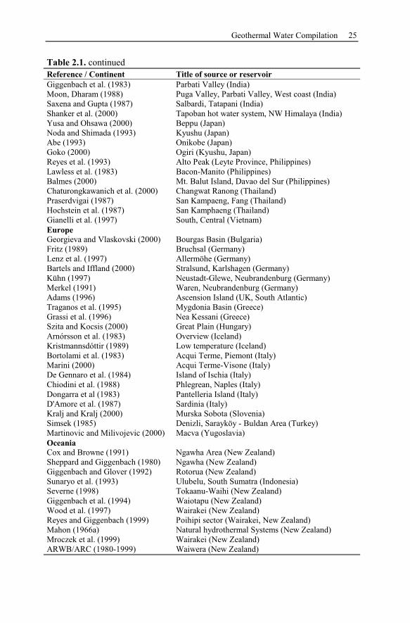
Geothermal Water Compilation 25
Table 2.1. continued
Reference / Continent Title of source or reservoir
Giggenbach et al. (1983) Parbati Valley (India)
Moon, Dharam (1988) Puga Valley, Parbati Valley, West coast (India)
Saxena and Gupta (1987) Salbardi, Tatapani (India)
Shanker et al. (2000) Tapoban hot water system, NW Himalaya (India)
Yusa and Ohsawa (2000) Beppu (Japan)
Noda and Shimada (1993) Kyushu (Japan)
Abe (1993) Onikobe (Japan)
Goko (2000) Ogiri (Kyushu, Japan)
Reyes et al. (1993) Alto Peak (Leyte Province, Philippines)
Lawless et al. (1983) Bacon-Manito (Philippines)
Balmes (2000) Mt. Balut Island, Davao del Sur (Philippines)
Chaturongkawanich et al. (2000) Changwat Ranong (Thailand)
Praserdvigai (1987) San Kampaeng, Fang (Thailand)
Hochstein et al. (1987) San Kamphaeng (Thailand)
Gianelli et al. (1997) South, Central (Vietnam)
Europe
Georgieva and Vlaskovski (2000) Bourgas Basin (Bulgaria)
Fritz (1989) Bruchsal (Germany)
Lenz et al. (1997) Allermöhe (Germany)
Bartels and Iffland (2000) Stralsund, Karlshagen (Germany)
Kühn (1997) Neustadt-Glewe, Neubrandenburg (Germany)
Merkel (1991) Waren, Neubrandenburg (Germany)
Adams (1996) Ascension Island (UK, South Atlantic)
Traganos et al. (1995) Mygdonia Basin (Greece)
Grassi et al. (1996) Nea Kessani (Greece)
Szita and Kocsis (2000) Great Plain (Hungary)
Arnórsson et al. (1983) Overview (Iceland)
Kristmannsdóttir (1989) Low temperature (Iceland)
Bortolami et al. (1983) Acqui Terme, Piemont (Italy)
Marini (2000) Acqui Terme-Visone (Italy)
De Gennaro et al. (1984) Island of Ischia (Italy)
Chiodini et al. (1988) Phlegrean, Naples (Italy)
Dongarra et al (1983) Pantelleria Island (Italy)
D'Amore et al. (1987) Sardinia (Italy)
Kralj and Kralj (2000) Murska Sobota (Slovenia)
Simsek (1985) Denizli, Sarayköy - Buldan Area (Turkey)
Martinovic and Milivojevic (2000) Macva (Yugoslavia)
Oceania
Cox and Browne (1991) Ngawha Area (New Zealand)
Sheppard and Giggenbach (1980) Ngawha (New Zealand)
Giggenbach and Glover (1992) Rotorua (New Zealand)
Sunaryo et al. (1993) Ulubelu, South Sumatra (Indonesia)
Severne (1998) Tokaanu-Waihi (New Zealand)
Giggenbach et al. (1994) Waiotapu (New Zealand)
Wood et al. (1997) Wairakei (New Zealand)
Reyes and Giggenbach (1999) Poihipi sector (Wairakei, New Zealand)
Mahon (1966a) Natural hydrothermal Systems (New Zealand)
Mroczek et al. (1999) Wairakei (New Zealand)
ARWB/ARC (1980-1999) Waiwera (New Zealand)
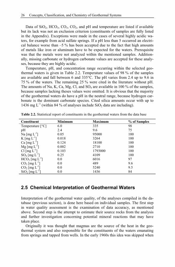
26 Concepts, Classification, and Chemistry of Geothermal Systems
Data of SiO2, HCO3, CO3, CO2, and pH and temperature are listed if available
but its lack was not an exclusion criterion (constituents of samples are fully listed
in the Appendix). Exceptions were made in the cases of several highly acidic wa-
ters, for example from acid sulfate springs. If a pH less than 5 occurred an electri-
cal balance worse than –5 % has been accepted due to the fact that high amounts
of metals like iron or aluminum have to be expected for the waters. Prerequisite
was that the metals were not analyzed within the mentioned samples. Addition-
ally, missing carbonate or hydrogen carbonate values are accepted for these analy-
ses, because they are highly acidic.
Temperature, pH, and concentration range occurring within the selected geo-
thermal waters is given in Table 2.2. Temperature values of 98 % of the samples
are available and fall between 6 and 335°C. The pH varies from 2.4 up to 9.6 in
75 % of the waters. The remaining 25 % were cited in the literature without pH.
The amounts of Na, K, Ca, Mg, Cl, and SO4 are available in 100 % of the samples,
because samples lacking theses values were omitted. It is obvious that the majority
of the geothermal waters do have a pH in the neutral range, because hydrogen car-
bonate is the dominant carbonate species. Cited silica amounts occur with up to
1436 mg L-1
(within 84 % of analyses include SiO2 data are including).
Table 2.2. Statistical report of constituents in the geothermal waters from the data base
Constituent Minimum Maximum % of Samples
Temperature [°C] 6.0 335 98
pH 2.4 9.6 75
Na [mg L-1
] 0.05 95000 100
K [mg L-1
] 0.018 3264 100
Ca [mg L-1
] 0.124 18100 100
Mg [mg L-1
] 0.002 2710 100
Cl [mg L-1
] 0.103 1793000 100
SO4 [mg L-1
] 0.25 4109 100
HCO3 [mg L-1
] 0.0 6016 97
CO3 [mg L-1
] 0.0 489 9.6
CO2 [mg L-1
] 0.0 5240 9.5
SiO2 [mg L-1
] 0.0 1436 84
2.5 Chemical Interpretation of Geothermal Waters
Interpretation of the geothermal water quality, of the analyses compiled in the da-
tabase (previous section), is done here based on individual samples. The first step
in water quality assessment is the examination of data accuracy, as mentioned
above. Second step is the attempt to estimate their source rocks from the analysis
and further investigation concerning potential mineral reactions that may have
taken place.
Originally it was thought that magmas are the source of the heat in the geo-
thermal system and also responsible for the constituents of the waters emanating
from springs and tapped from wells. In the early 1960s this idea was skipped when
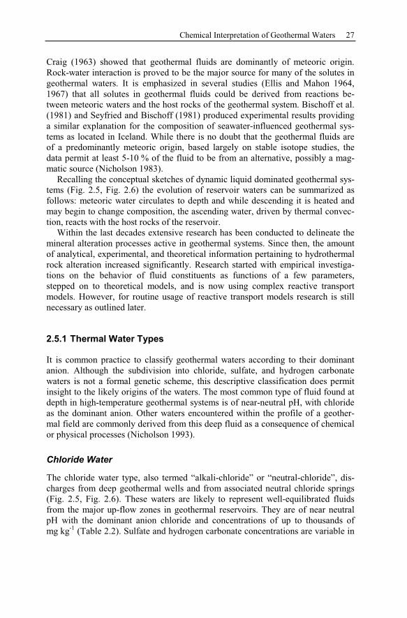
Chemical Interpretation of Geothermal Waters 27
Craig (1963) showed that geothermal fluids are dominantly of meteoric origin.
Rock-water interaction is proved to be the major source for many of the solutes in
geothermal waters. It is emphasized in several studies (Ellis and Mahon 1964,
1967) that all solutes in geothermal fluids could be derived from reactions be-
tween meteoric waters and the host rocks of the geothermal system. Bischoff et al.
(1981) and Seyfried and Bischoff (1981) produced experimental results providing
a similar explanation for the composition of seawater-influenced geothermal sys-
tems as located in Iceland. While there is no doubt that the geothermal fluids are
of a predominantly meteoric origin, based largely on stable isotope studies, the
data permit at least 5-10 % of the fluid to be from an alternative, possibly a mag-
matic source (Nicholson 1983).
Recalling the conceptual sketches of dynamic liquid dominated geothermal sys-
tems (Fig. 2.5, Fig. 2.6) the evolution of reservoir waters can be summarized as
follows: meteoric water circulates to depth and while descending it is heated and
may begin to change composition, the ascending water, driven by thermal convec-
tion, reacts with the host rocks of the reservoir.
Within the last decades extensive research has been conducted to delineate the
mineral alteration processes active in geothermal systems. Since then, the amount
of analytical, experimental, and theoretical information pertaining to hydrothermal
rock alteration increased significantly. Research started with empirical investiga-
tions on the behavior of fluid constituents as functions of a few parameters,
stepped on to theoretical models, and is now using complex reactive transport
models. However, for routine usage of reactive transport models research is still
necessary as outlined later.
2.5.1 Thermal Water Types
It is common practice to classify geothermal waters according to their dominant
anion. Although the subdivision into chloride, sulfate, and hydrogen carbonate
waters is not a formal genetic scheme, this descriptive classification does permit
insight to the likely origins of the waters. The most common type of fluid found at
depth in high-temperature geothermal systems is of near-neutral pH, with chloride
as the dominant anion. Other waters encountered within the profile of a geother-
mal field are commonly derived from this deep fluid as a consequence of chemical
or physical processes (Nicholson 1993).
Chloride Water
The chloride water type, also termed “alkali-chloride” or “neutral-chloride”, dis-
charges from deep geothermal wells and from associated neutral chloride springs
(Fig. 2.5, Fig. 2.6). These waters are likely to represent well-equilibrated fluids
from the major up-flow zones in geothermal reservoirs. They are of near neutral
pH with the dominant anion chloride and concentrations of up to thousands of
mg kg-1
(Table 2.2). Sulfate and hydrogen carbonate concentrations are variable in
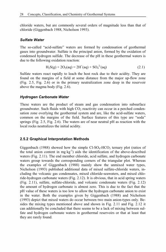
28 Concepts, Classification, and Chemistry of Geothermal Systems
chloride waters, but are commonly several orders of magnitude less than that of
chloride (Giggenbach 1988, Nicholson 1993).
Sulfate Water
The so-called “acid-sulfate” waters are formed by condensation of geothermal
gases into groundwater. Sulfate is the principal anion, formed by the oxidation of
condensed hydrogen sulfide. The decrease of the pH in these geothermal waters is
due to the following oxidation reaction:
H2S(g) + 2O2(aq) = 2H+(aq) + SO4
2-(aq) (2.1)
Sulfate waters react rapidly to leach the host rock due to their acidity. They are
found on the margins of a field at some distance from the major up-flow zone
(Fig. 2.5, Fig. 2.6) or in the primary neutralization zone deep in the reservoir
above the magma body (Fig. 2.6).
Hydrogen Carbonate Water
These waters are the product of steam and gas condensation into subsurface
groundwater. Such fluids with high CO2 reactivity can occur in a perched conden-
sation zone overlying the geothermal system and are, like the acid-sulfate waters,
common on the margins of the field. Surface features of this type are “soda”
springs (Fig. 2.5, Fig. 2.6). The waters are of near neutral pH as reaction with the
local rocks neutralizes the initial acidity.
2.5.2 Graphical Interpretation Methods
Giggenbach (1988) showed how the simple Cl-SO4-HCO3 ternary plot (ratios of
the total anion content in mg kg-1
) aids the identification of the above-described
waters (Fig. 2.11). The end member chloride, acid sulfate, and hydrogen carbonate
waters group towards the corresponding corners of the triangular plot. Whereas
the examples of Giggenbach (1988) mainly show the unmixed water types,
Nicholson (1993) published additional data of mixed sulfate-chloride waters, in-
cluding the volcanic gas condensates, mixed chloride-seawaters, and mixed chlo-
ride-hydrogen carbonate waters (Fig. 2.12). It is obvious, that in acid spring waters
(Fig. 2.11), sulfate, sulfate-chloride, and volcanic condensate waters (Fig. 2.12)
the amount of hydrogen carbonate is almost zero. This is due to the fact that the
pH value of these waters is too low to allow the hydrogen carbonate anion to exist
in the water. Both the examples given by Giggenbach (1988) and Nicholson
(1993) depict that mixed waters do occur between two main anion-types only. Be-
sides the mixing types mentioned above and shown in Fig. 2.11 and Fig. 2.12 it
can additionally be concluded that there seems to be a lack of mixing between sul-
fate and hydrogen carbonate waters in geothermal reservoirs or that at least that
they are rarely found.
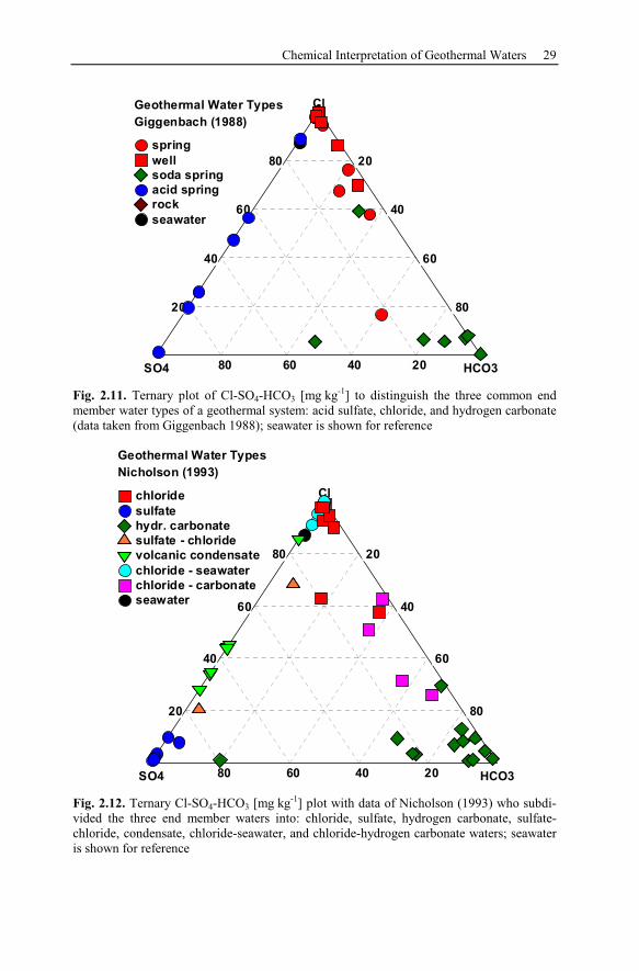
Chemical Interpretation of Geothermal Waters 29
80 60 40 20
20
40
60
80 20
40
60
80
SO4 HCO3
ClGeothermal Water Types
Giggenbach (1988)
spring
well
soda spring
acid spring
rock
seawater
Fig. 2.11. Ternary plot of Cl-SO4-HCO3 [mg kg-1
] to distinguish the three common end
member water types of a geothermal system: acid sulfate, chloride, and hydrogen carbonate
(data taken from Giggenbach 1988); seawater is shown for reference
80 60 40 20
20
40
60
80 20
40
60
80
SO4 HCO3
Cl
Geothermal Water Types
Nicholson (1993)
chloride
sulfate
hydr. carbonate
sulfate - chloride
volcanic condensate
chloride - seawater
chloride - carbonate
seawater
Fig. 2.12. Ternary Cl-SO4-HCO3 [mg kg-1
] plot with data of Nicholson (1993) who subdi-
vided the three end member waters into: chloride, sulfate, hydrogen carbonate, sulfate-
chloride, condensate, chloride-seawater, and chloride-hydrogen carbonate waters; seawater
is shown for reference
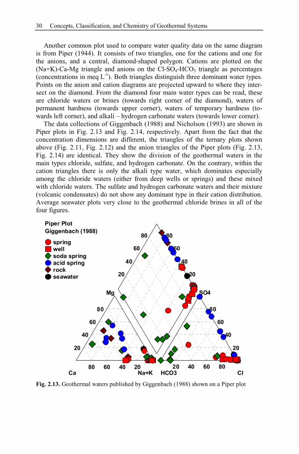
30 Concepts, Classification, and Chemistry of Geothermal Systems
Another common plot used to compare water quality data on the same diagram
is from Piper (1944). It consists of two triangles, one for the cations and one for
the anions, and a central, diamond-shaped polygon. Cations are plotted on the
(Na+K)-Ca-Mg triangle and anions on the Cl-SO4-HCO3 triangle as percentages
(concentrations in meq L-1
). Both triangles distinguish three dominant water types.
Points on the anion and cation diagrams are projected upward to where they inter-
sect on the diamond. From the diamond four main water types can be read, these
are chloride waters or brines (towards right corner of the diamond), waters of
permanent hardness (towards upper corner), waters of temporary hardness (to-
wards left corner), and alkali – hydrogen carbonate waters (towards lower corner).
The data collections of Giggenbach (1988) and Nicholson (1993) are shown in
Piper plots in Fig. 2.13 and Fig. 2.14, respectively. Apart from the fact that the
concentration dimensions are different, the triangles of the ternary plots shown
above (Fig. 2.11, Fig. 2.12) and the anion triangles of the Piper plots (Fig. 2.13,
Fig. 2.14) are identical. They show the division of the geothermal waters in the
main types chloride, sulfate, and hydrogen carbonate. On the contrary, within the
cation triangles there is only the alkali type water, which dominates especially
among the chloride waters (either from deep wells or springs) and these mixed
with chloride waters. The sulfate and hydrogen carbonate waters and their mixture
(volcanic condensates) do not show any dominant type in their cation distribution.
Average seawater plots very close to the geothermal chloride brines in all of the
four figures.
80 60 40 20 20 40 60 80
20
40
60
80 80
60
40
20
20
40
60
80
20
40
60
80
Ca Na+K HCO3 Cl
Mg SO4
Piper Plot
Giggenbach (1988)
spring
well
soda spring
acid spring
rock
seawater
Fig. 2.13. Geothermal waters published by Giggenbach (1988) shown on a Piper plot
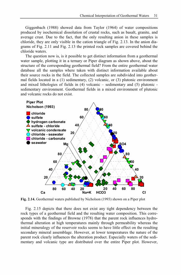
Chemical Interpretation of Geothermal Waters 31
Giggenbach (1988) showed data from Taylor (1964) of water compositions
produced by isochemical dissolution of crustal rocks, such as basalt, granite, and
average crust. Due to the fact, that the only resulting anion in these samples is
chloride, they are only visible in the cation triangle of Fig. 2.13. In the anion dia-
grams of Fig. 2.11 and Fig. 2.13 the printed rock samples are covered behind the
chloride waters.
The question now is, is it possible to get distinct information from a geothermal
water sample, plotting it in a ternary or Piper diagram as shown above, about the
structure of the corresponding geothermal field? From the entire geothermal water
database all the samples where taken with distinct information available about
their source rocks in the field. The collected samples are subdivided into geother-
mal fields located in a (1) sedimentary, (2) volcanic, or (3) plutonic environment
and mixed lithologies of fields in (4) volcanic – sedimentary and (5) plutonic -
sedimentary environment. Geothermal fields in a mixed environment of plutonic
and volcanic rocks do not exist.
80 60 40 20 20 40 60 80
20
40
60
80 80
60
40
20
20
40
60
80
20
40
60
80
Ca Na+K HCO3 Cl
Mg SO4
Piper Plot
Nicholson (1993)
chloride
sulfate
hydrogen carbonate
sulfate - chloride
volcanic condensate
chloride - seawater
chloride - carbonate
seawater
Fig. 2.14. Geothermal waters published by Nicholson (1993) shown on a Piper plot
Fig. 2.15 depicts that there does not exist any tight dependency between the
rock types of a geothermal field and the resulting water composition. This corre-
sponds with the findings of Browne (1978) that the parent rock influences hydro-
thermal alteration at high temperatures mainly through permeability whereas the
initial mineralogy of the reservoir rocks seems to have little effect on the resulting
secondary mineral assemblage. However, at lower temperatures the nature of the
parent rock clearly influences the alteration product. Especially waters of the sedi-
mentary and volcanic type are distributed over the entire Piper plot. However,
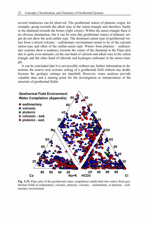
32 Concepts, Classification, and Chemistry of Geothermal Systems
several tendencies can be observed. The geothermal waters of plutonic origin, for
example, group towards the alkali type in the cation triangle and therefore finally
in the diamond towards the brines (right corner). Within the anion triangle there is
no obvious domination, but it can be seen that geothermal waters of plutonic ori-
gin do not show the acid sulfate type. The dominant cation type of geothermal wa-
ters from a mixed volcanic - sedimentary environment seems to be of the calcium
cation-type and often of the sulfate-anion type. Waters from plutonic – sedimen-
tary systems show a tendency towards the center of the diamond in the Piper plot
due to quite even amounts, on the one hand of calcium and alkali ions in the cation
triangle and the other hand of chloride and hydrogen carbonate in the anion trian-
gle.
It can be concluded that it is not possible without any further information to de-
termine the source rock tectonic setting of a geothermal field without any doubt,
because the geologic settings are manifold. However, water analyses provide
valuable data and a starting point for the investigation or interpretation of the
structure of geothermal fields.
80 60 40 20 20 40 60 80
20
40
60
80 80
60
40
20
20
40
60
80
20
40
60
80
Ca Na+K HCO3 Cl
Mg SO4
Geothermal Field Environment
Water Compilation (Appendix)
sedimentary
volcanic
plutonic
volcanic - sed.
plutonic - sed.
Fig. 2.15. Piper plot of the geothermal water compilation subdivided into waters from geo-
thermal fields in sedimentary, volcanic, plutonic, volcanic – sedimentary, or plutonic - sedi-
mentary environment
Processes Affecting the Chemical Composition of Hydrothermal Waters 33
2.6 Processes Affecting the Chemical Composition of
Hydrothermal Waters
The contemplation of processes affecting the chemical composition of hydrother-
mal waters is done here distinguishing between reactions playing a dominant role
in dynamic magmatic systems of high temperature and static or dynamic sediment
hosted systems of low temperature (Fig. 2.2). Both groups are important for un-
derstanding the structure of geothermal reservoirs.
2.6.1 Dynamic Magmatic Systems (High-Temperature)
Reactions of thermal waters with rocks are called hydrothermal alteration. Hydro-
thermal alteration involves mineralogical, chemical and textural changes. Due to
the fact that alteration reactions depend on the particular conditions of temperature
and pressure, they are prevailed by the temporal and local development of the
physical conditions in hydrothermal systems.
Chemical and physical processes influence the composition of both the mete-
oric water as it descends into the reservoir and the geothermal water as it ascends
through the up-flow zone to the surface (Fig. 2.1 and Fig. 2.4 - Fig. 2.6). The main
chemical processes are mineral dissolution and precipitation, while the dominant
physical process is boiling, although conductive cooling and mixing are also im-
portant.
Constituents of thermal waters can be divided into the soluble or non-reactive
group (e.g. Cl, B, Br, etc.) and the rock-forming species (e.g. SiO2, Na, K, Ca, Mg,
etc.) providing the basis for water classification (see above) and reservoir interpre-
tation. Solubility of the rock-forming species is controlled by mineral-fluid equi-
libria. The reactions, which take place, are a function of temperature, pressure, sa-
linity, and host rock composition of the geothermal system (Nicholson 1993). The
product of mineral-fluid reactions is an assemblage of secondary alteration miner-
als discussed in detail by Browne (1978) and Giggenbach (1981, 1984, 1988).
The physical and chemical conditions of recent dynamic hydrothermal altera-
tion systems can be applied to the situation of fossil systems. The overall fluid-
rock equilibrium is rarely attained and the fluids are likely to have reached some
complex steady-state composition at particular locations. Compared to a composi-
tion in thermodynamic equilibrium, representing the most stable mineral assem-
blage and water composition, a steady-state is characterized by constant values of
metastable reaction intermediates within a dynamic equilibrium. Any specific
composition reflects the combined effects of initial fluid constituents, kinetics of
primary mineral dissolution and secondary mineral deposition at changing tem-
peratures and pressures, vapor loss, dilution, and mixing with fluids of different
origin. Two end member processes determine the actual state of chemical equilib-
rium or non-equilibrium in the hydrothermal system. The reaction sequence starts
34 Concepts, Classification, and Chemistry of Geothermal Systems
with (1) isochemical dissolution (in proportions of the original rock) of the rock
material in contact with the rising fluid, a more or less hypothetical process and
eventually ends with (2) equilibration of the fluid in respect to the thermodynami-
cally stable alteration assemblage resulting from recrystallization of primary rock
at a given temperature and pressure, a process likely to come to completion only
in stagnant systems of infinite age (Giggenbach 1984, 1988).
Following the concept of dynamic magmatic high temperature systems within a
low relief setting (Fig. 2.6) the hydrothermal alteration processes are distinguished
here in (1) Na-Mg-Ca-metasomatism or propylitic alteration at the periphery of
the system occurring due to descending meteoric waters (metasomatism: the en-
richment or depletion of a system in an element or elements by an externally-
derived fluid). Subsequently the deep circulating geothermal water may experi-
ence (2) H-metasomatism or argillic alteration in the so called primary neutraliza-
tion zone due to the attack of strong acids like HCl, H2SO4, and HF from the de-
gassing magma body. The very slow drop of temperature over deeper, central
parts of the major fluid up-flow zone leads to (3) K-metasomatism or potassic al-
teration characterized by isochemical recrystallization of the rock components. K-
metasomatism is often accompanied by (4) silicification or silication. The fluids
emerging from the neutralization zone still contain magmatic CO2 and H2S, hence
(5) H-metasomatism proceeds by CO2 attack on Ca-aluminum silicates in a secon-
dary neutralization of CO2. K-metasomatism and H-metasomatism are superim-
posed in the region of (6) H-K-metasomatism or phyllic alteration (scheme (1)-(6)
is also applicable for other dynamic magmatic systems).
Propylitic Alteration (Na-Mg-Ca-Metasomatism)
Propylite is an old term used to describe altered volcanic rocks. Propylitic altera-
tion, especially occurring in zones of descending meteoric waters in the hydro-
thermal system (or seawater in geothermal fields like Iceland) as stated by Gig-
genbach (1988), is characterized by the addition of H2O and CO2, and locally S,
but without appreciable H-metasomatism. The meteoric water entering the hydro-
thermal system at the periphery (recharge zone) is heated and undergoes Na-Mg-
Ca-metasomatism. Potassium minerals, like the K-feldspar microcline (KAlSi3O8),
are preferentially destroyed on contact with descending solutions leading to the
formation of assemblages containing albite (NaAlSi3O8), chlorite
((Mg,Fe,Al)6(Al,Si)4O10(OH)8), and epidote (Ca2FeAl2Si3 O12 (OH)). It can be said
that downward flow and increasing temperatures favor assemblages containing
minerals more soluble at low temperatures.
Argillic Alteration (H-Metasomatism)
Argillic alteration is characterized by the formation of clay minerals due to intense
H-metasomatism, also called acid leaching. As stated above, H-metasomatism
may occur within the hydrothermal system in two different cases, either deep in
the reservoir within the primary neutralization zone or adjacent to the main up-
flow region within the secondary neutralization zone (Fig. 2.6).
Processes Affecting the Chemical Composition of Hydrothermal Waters 35
H-metasomatism is a widespread and very important type of reaction in hydro-
thermal alteration processes. It is based on the hydrolysis of H2O into H+ and OH
-,
with the consumption of H+ during reaction with silicate minerals and release of
metal ions into the water. Hydration, the transfer of molecular water from the so-
lution to a mineral, often accompanies hydrolysis. The alteration of olivine
(Mg2SiO4) to serpentine (Mg3Si2O5(OH)4) outlines the consumption of H+, the re-
lease of Mg2+
and the incorporation of molecular water as an example.
2 Mg2SiO4 + H2O + 2 H+ ⇔ Mg3Si2O5(OH)4 + Mg
2+(2.2)
Argillic alteration may be subdivided on the basis of the composition of the geo-
logical formations undergoing H-metasomatism, specifically rocks:
• dominated by feldspars,
• with a prevailing mafic composition, or
• rich in calcium, like carbonates.
Within hydrothermal reservoirs, the circulating geothermal water may absorb
strong acids like HCl, H2SO4, and HF from the deep magmatic to hydrothermal
transition zone. This is a reaction most likely to occur but impossible to observe
directly. The absorption of magmatic vapor into the deeply circulating fluid leads
to initial rock dissolution. The vapor composition can be estimated of high tem-
perature gases released from basaltic (Giggenbach and Le Guern 1976) or ande-
sitic magmas (Giggenbach 1987). Magma gases contain 20-40 wt.% CO2, 5-10 %
b.w. total sulfur, predominantly in the form of SO2 at low pressures, but H2S at
higher pressures, and 1-2 % b.w. HCl (Rose et al. 1986). The passage of the geo-
thermal water through the neutralization zone results firstly in an increase of Na,
K, Mg, and Ca due to almost isochemical rock dissolution. Secondly, still in the
neutralization zone, the amounts of Ca and Mg subsequently decrease by forma-
tion of alteration products like amphiboles [e.g. anhydrite (CaSO4), biotite, chlo-
rite (K(Mg,Fe)3AlSi3O10(OH)2), tremolite (Ca2(Mg,Fe)4AlSi7AlO22(OH)2), or fluo-
rite (CaF2)].
The fluids emerging from the neutralization zone still contain magmatic CO2
and H2S leading to H-metasomatism adjacent to the up-flow region. The CO2 at-
tack on Ca-aluminum silicates, a more gentle reaction [Eq. (2.3)], leads to the
conversion of carbon dioxide to calcite (CaCO3) and “acid” clays
Ca-Al-silicate + CO2 + H2O ⇔ CaCO3 + 2(H-Al-silicate) (2.3)
and subsequently to “neutral” aluminum silicates (z = stoichiometric factor):
z(H-Al-silicate) + Mz+ ⇔ (M-Al-silicate) + zH
+(2.4)
H-Metasomatism of Feldspars. Hemley and Jones (1964) conducted experimen-
tal studies of reactions between feldspars and sodium chloride solutions. Investi-
gating the K2O-Al2O3-SiO2-H2O system, an example is given here of the conver-
sion of the anhydrous silicate K-feldspar microcline (KAlSi3O8) to the hydrous K-
mica sericite (KAl3Si3O10(OH)2) during quartz (SiO2) formation. Sericite is a
varietal name used for fine-grained muscovite, illite or paragonite.
36 Concepts, Classification, and Chemistry of Geothermal Systems
3 KAlSi3O8 + 2 H+ ⇔ KAl3Si3O10(OH)2 + 2 K
+ + 6 SiO2 (2.5)
The reaction of andesine (Na2CaAl4Si8O24) to K-mica due to argillic alteration dis-
plays H-metasomatism intersecting with K-metasomatism (see below).
3 Na2CaAl4Si8O24 + 8 H+ + 4 K
+ ⇔4 KAl3Si3O10(OH)2 + 6 Na
+ + 3 Ca
2+ + 12 SiO2
(2.6)
Successive reactions following the development of K-mica may be, due to further
H-metasomatism, the occurrence of kaolinite (Al2Si2O5(OH)4) or pyrophyllite
(Al2Si4O10(OH)2). Low temperatures and low cation / H+ ratios support the devel-
opment of kaolinite (Meyer and Hemley 1967).
2 KAl3Si3O10(OH)2 + 2 H+ + 3 H2O ⇔ 3 Al2Si2O5(OH)4 + 2 K
+(2.7)
2 KAl3Si3O10(OH)2 + 2 H+ + 6 SiO2 ⇔ 3 Al2Si4O10(OH)2 + 2 K
+(2.8)
The patterns of argillic alteration within the system Na2O-Al2O3-SiO2-H2O are
transferable to the reactions of K-feldspars. Albite (NaAlSi3O8) the counterpart to
microcline for example converts to paragonite (NaAl3Si3O10(OH)2) the sodium
counterpart to K-micas and due to further H-metasomatism within a successive re-
action also to pyrophillite.
Processes within the system K2O-Al2O3-SiO2-H2O-SO3 are prevailed by the
formation of sulfuric acid due to the oxidation of H2S [Eq. (2.1)]. Hemley et al.
(1969) experimentally studied this five component system with special considera-
tion of the stability of K-feldspars, muscovite (KAl3Si3O10(OH)2), kaolinite and
alunite (KAl3(SO4)2(OH)6). Alunite is a key mineral within this system and is of-
ten found in sulfur-rich epithermal gold-silver deposits (Pirajno 1992). The min-
eral assemblage is determined by the following reactions of K-feldspar to alunite
[Eq. (2.9)], K-mica to alunite [Eq. (2.10)] or kaolinite [Eq. (2.11)] and the conver-
sion of muscovite to kaolinite [Eq. (2.12)].
3 KAlSi3O8 + 6 H+ + 2 SO4
2- ⇔ KAl3(SO4)2(OH)6 + 2 K+ + 9 SiO2 (2.9)
KAl3Si3O10(OH)2 + 4 H+ + 2 SO4
2- ⇔ KAl3(SO4)2(OH)6 + 3 SiO2 (2.10)
3 Al2Si2O5(OH)4 + 2 K+ + 6 H
+ + 4 SO4
2- ⇔2 KAl3(SO4)2(OH)6 + 6 SiO2 + 3 H2O
(2.11)
2 KAl3Si3O10(OH)2 + 2 H+ + 3 H2O ⇔ 3 Al2Si2O5(OH)4 + 2 K
+(2.12)
H-Metasomatism of Mafic Rocks. Hydrothermal alteration of mafic rocks is spa-
tially related to the occurrence of basaltic formations, for example at mid ocean
ridge spreading centers or continental rift settings. The group of mafic minerals is,
in general, comprised of Fe-Mg silicates like biotite (K(Mg,Fe)3AlSi3O10(OH,F)2),
amphiboles ((Ca,Na)2(Mg,Fe,Al)5Si8O22(OH)2), pyroxenes (orthopyroxene:
Processes Affecting the Chemical Composition of Hydrothermal Waters 37
(Mg,Fe)2Si2O6), clinopyroxenes (Ca(Mg,Fe)Si2O6 – Na(Al,Fe)Si2O6), or olivine
((Mg,Fe)2SiO4).
Hydrothermal activity in sub-sea floor systems is a typical environment for the
alteration of mafic rocks. The penetration and descent of seawater through frac-
tures in the oceanic crust leads to heating of the solutions which become more and
more reduced due to reactions with the rock forming minerals. A typical reaction
is the H-metasomatism of fayalite (Fe2SiO4) to magnetite (Fe3O4) and pyrite
(FeS2).
11 Fe2SiO4 + 2 SO4
2- + 4 H
+ ⇔ 7 Fe3O4 + FeS2 + 11 SiO2 + 2 H2O (2.13)
Hydrothermal reactions at spreading centers are described in detail by Edmond
and Damm (1983).
H-metasomatism in Ca-Rich Environments. Hydrogen ion metasomatism of
carbonates is mainly described for the dissolution of calcite and the production of
carbon dioxide resulting in the formation of carbonic acid (H2CO3).
CaCO3 + 2 H+ ⇔ Ca
2+ + CO2 + H2O ⇔ Ca
2+ + H2CO3 (2.14)
The carbonic acid dissociation in turn leads to hydrolysis of silicates, forming
clays and liberating silica and metal ions.
Potassic Alteration (K-Metasomatism)
Potassic alteration or K-metasomatism describes exchange reactions in feldspars,
specifically Na for K, or K for Na, which in the latter case is called sodium altera-
tion. Both types of exchange are combined under the name of alkali metasoma-
tism. These exchange reactions, with the first one predominant in hydrothermal
systems, results in changes of the structural state of the feldspars. This is not to be
confused with ion exchange on surfaces where only physical processes occur in
contrary to the chemical reactions of alkali metasomatism.
H-metasomatism is subject to rapid conductive cooling or dilution, adjacent to
the major up-flow zone and culminating in waters high in hydrogen carbonate,
whereas potassium metasomatism occurs in the major up-flow zone (Fig. 2.6). K-
metasomatism is the predominant process occurring with the cooling of ascending
solutions and is accompanied by silification (see below) and characterized by the
formation of K-feldspar, biotite, K-mica or K-rich clays.
Potassic alteration is important in porphyry and epithermal mineralizing sys-
tems. The minerals, which are characteristic for K-metasomatism, are K-feldspar
and biotite in porphyries, and adularia in epithermal systems. Sulfides like chal-
copyrite, pyrite, and molybdenite normally occur due to potassic alteration. In por-
phyry regions, anhydrite is a common accompanying mineral phase (Pirajno
1992).
The very slow drop of temperature within deeper, central parts of the major
fluid up-flow zone leads to recrystallization of rock components over close to
stagnant parts of the system and the attainment of full water-rock equilibrium.
Waters from deep geothermal wells appear to achieve compositions close to full
38 Concepts, Classification, and Chemistry of Geothermal Systems
water-rock equilibrium with respect to the reaction of albite (Na-feldspar,
NaAlSi3O8) and K-feldspar (e.g. microcline).
Na-feldspar + K+ ⇔ K-feldspar + Na
+(2.15)
Phyllic Alteration (H-K Metasomatism)
The regions of K-metasomatism and H-metasomatism are superimposed and com-
bined under the term of phyllic or sericitic alteration. This is one of the most
common types of hydrothermal alteration, present not only in Archean volcano-
genic but also in recent epithermal systems, responsible for massive sulfide and
gold-quartz deposits. A typical mineral assemblage for phyllic alteration zones
consists of quartz, sericite, and pyrite accompanied by minerals like K-feldspar,
kaolinite, calcite, biotite, rutile (TiO2), apatite (Ca5(PO4)3(OH,F,Cl)), and anhy-
drite. Phyllic alteration spreads into the potassic type by increasing amounts of K-
feldspars and into the argillic type by increasing amounts of clay-minerals (Fig.
2.6, Pirajno 1992).
Giggenbach (1984) stated, accepting fluid and mineral compositions resulting
from recrystallization of the parent rock, that a fully equilibrated system corre-
sponds to K-feldspar / K-layer silicate coexistence. For different temperatures,
theoretical CO2 fugacities may be evaluated. For temperatures up to 200°C this is
done taking the reaction between laumontite (CaAl2Si4O12
.4H2O), microcline, car-
bon dioxide, calcite (CaCO3), muscovite (KAl3Si3O10(OH)2), and silica.
laumontite + microcline + CO2 ⇔calcite + muscovite + 4 SiO2
(2.16)
For temperatures from 200 to 280°C the dominant reaction is between clinozoisite
(Ca2Al3Si3O12(OH)), microcline, carbon dioxide, calcite, muscovite and silica.
2 clinozoisite + 3 microcline + CO2 ⇔calcite + 3 muscovite + 6 SiO2
(2.17)
At even higher temperatures, wairakite (CaAl2Si4O12
.H2O)
wairakite + microcline + CO2 ⇔calcite + muscovite + 4 SiO2
(2.18)
or anorthite (CaAl2Si2O8) control the reaction.
anorthite + microcline + CO2 ⇔calcite + muscovite + 2 SiO2
(2.19)
Silicification
The best-known and probably most common type of alteration is silicification.
During hydrothermal processes silica may either be introduced from the circulat-
ing fluids and precipitated due to its prograde solubility or left behind in the form
Processes Affecting the Chemical Composition of Hydrothermal Waters 39
of residual silica as shown for H-metasomatism of feldspars [Eqs. (2.5), (2.6),
(2.9) - (2.11)] or mafic rocks [Eq. (2.13)] and the region of H-K-metasomatism
[Eqs. (2.16)-(2.19)].
Silication
Silication results in skarn rocks, in which the addition of silica leads to the devel-
opment of calc-silica minerals. Skarns develop at the contact between plutons with
carbonate rocks. Skarns are very important because they host a great variety of
ores. Silication is the replacement of carbonate rocks by silicate minerals like the
reaction of calcite or dolomite to wollastonite (CaSiO3) or diopside
((CaMg)Si2O6), respectively.
CaCO3 + SiO2 ⇔ CaSiO3 + CO2 (2.20)
CaMg(CO3)2 + 2 SiO2 ⇔ (CaMg)Si2O6 + 2 CO2 (2.21)
2.6.2 Static and Dynamic Sediment Hosted Systems (Low
Temperature)
The groundwaters in deep sedimentary basins are characterized by long residence
times (static system) and the variable mineralogical composition of host rocks and
matrix. The North German basin is an example of the occurrence of hydrothermal
waters in a static system. Müller and Papendieck (1975) described in detail the
genesis of these deep-seated brines. The majority of geothermal waters in the
North German basin are low (36 – 150 g L-1
total dissolved solids) to high concen-
trated (280 – 360 g L-1
). For the origin and evolution of the brines the following
processes have to be taken into account separately or in various combinations:
• Evaporation under surface conditions leading to highly saline brines as by-
products. These so called "relict" solutions may remain within the sediments
during diagenesis.
• Compaction driven flow of pressurized formation waters and their diagentic al-
teration.
• Meteoric water intrusion in regions containing evaporites resulting in dissolu-
tion of rock salts and the formation of brines.
From intensive evaporation of marine or continental waters salt solutions result
at the Earth's surface from which evaporites evolve. Evaporite deposits are impor-
tant sources of gypsum, halite, and other economically significant minerals. Salts
commonly resulting from evaporite evolution of marine origin, composed of the
major seawater ions, are given in Table 2.3.
The inherent processes of evaporite evolution from seawater are described by
Hardie and Eugster (1970) and Hardie (1996). Spencer et al. (1985a, 1985b) de-
scribed the relationship between hydrology, salinity, and geochemistry of a conti-
nental evaporite system, the Great Salt Lake basin in Utah. Lerman (1979), Berner
40 Concepts, Classification, and Chemistry of Geothermal Systems
(1980), and Boudreau (1997) summarized the role of solute fluxes in and out of
pore fluids in aquatic sediments.
Table 2.3. Minerals found in evaporite deposits of marine origin
Mineral Formula Mineral Formula
anhydrite CaSO4 hexahydrite MgSO4·6H2O
bischofite MgCl2·6H2O kainite KMgClSO4·3H2O
bloedite Na2Mg(SO4)2·4H2O kieserite MgSO4·H2O
calcite CaCO3 mirabilite Na2SO4·10H2O
carnallite KMgCl3·6H2O polyhalite K2MgCa2(SO4)4
dolomite CaMg(CO3)2 sylvite KCl
glauberite Na2Ca(SO4)2 tachyhydrite Mg2CaCl6·12H2O
gypsum CaSO4·2H2O thenardite Na2SO4
halite NaCl trona Na3H(CO3)2·2H2O
Once evaporites are deposited and start to undergo burial, their physical and
hydraulic properties begin to change. Burial compacts the layered evaporites and
reduces their porosity. The interstitial brine is forced upward opposite the down-
ward movement of the sediment, into overlying strata. The brines buried within
their new host sediments start to react towards chemical equilibrium with the host
rocks and cement minerals.
The layered salt bodies tend to bulge upwards through overlying sediments
when they are deeply buried, because the contrast between their density (2200 kg
m-3
) and the density of the surrounding sediments (2500 kg m-3
) leads to unstable
conditions. The upward migration of salt is accompanied by a reciprocal down-
ward sagging of the surrounding sediments. The salt focuses itself into diapirs or
even salt dikes. Salt domes often exist in great numbers in basins that contain
deeply buried evaporites (e.g. North German basin). The existing salt structures
greatly affect the surrounding groundwater composition, minerals are leached, and
conversely the waters influence diagenesis and dissolution of the salt. As shown,
for example, by Kühn et al. (2002a) for the geothermal Buntsandstein reservoir of
Stralsund (Germany), the formation water is in thermodynamic equilibrium with
respect to the matrix minerals calcite and anhydrite. Within the Rhaetian reservoir
of Neustadt-Glewe (Germany) barite is in equilibrium with the highly saline brine
for reservoir conditions (Kühn 1997).
The possible processes listed above leading to highly saline geothermal brines
in deep-seated sedimentary rocks depend chiefly on the regional geology and geo-
logic structure of the system and can not be interpreted like geothermal waters
from the elucidated dynamic systems.
2.7 Geothermometer
Geothermometry is the use of a fluid's chemical composition to estimate the tem-
perature at which it equilibrated in the subsurface. It is an important tool in explor-
ing for and exploiting geothermal fields and for understanding the genesis of ore
Geothermometer 41
deposits. Generally, geothermometers are applied to characterize deep groundwa-
ter flow systems.
Chemical geothermometers are used to reconstruct thermal and chemical condi-
tions within deep structures of hydrothermal systems. They keep characteristics of
the temperature conditions prevailing within geothermal reservoirs in element
amounts or ratios of constituents. Based on water-rock equilibration reactions they
enable estimation of the reservoir temperature or maximum depth of circulation of
fluid on condition that (Nicholson 1993):
• element concentrations or species used for calculation are controlled by a tem-
perature-dependent water-rock equilibrium,
• there is an abundance of the mineral in the geothermal system,
• the considered reaction reaches equilibrium in the reservoir,
• there is no re-equilibration during flow of the reservoir fluid to the surface,
• there is no mixing or dilution of the deep fluid (in the case that the
geothermometer relies on absolute abundances).
The number of components involved in the chemical reactions occurring in
geothermal reservoirs can be used to subdivide the range of geothermometers. The
simplest ones are those based on univariant reactions like the silica geothermome-
ter. Mahon (1966b) recognized the relationship between the silica content in the
water with respect to a particular mineral phase and the reservoir temperature. In
the last decades this geothermometer has been refined resulting in the following
equations [Eqs. (2.22)-(2.26)] for varying silica modifications with the SiO2 con-
centration in mg kg-1
and temperatures below 250°C (Nicholson 1993):
[ ]( )
2
1309T C 273 (quartz, no steam loss)
5.19 log SiO
° = −−
(2.22)
[ ]( )
2
1032T C 273 (chalcedony)
4.69 log SiO
° = −−
(2.23)
[ ]( )
2
1000T C 273 ( cristobalite)
4.78 log SiO
° = − α −−
(2.24)
[ ]( )
2
781T C 273 ( cristobalite)
4.51 log SiO
° = − β −−
(2.25)
[ ]( )
2
731T C 273 (amorphous silica)
4.52 log SiO
° = −−
(2.26)
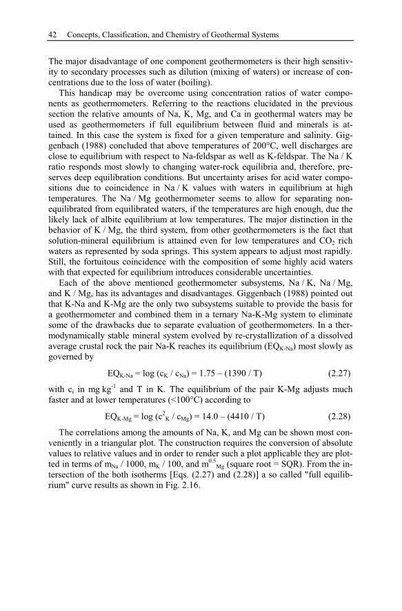
42 Concepts, Classification, and Chemistry of Geothermal Systems
The major disadvantage of one component geothermometers is their high sensitiv-
ity to secondary processes such as dilution (mixing of waters) or increase of con-
centrations due to the loss of water (boiling).
This handicap may be overcome using concentration ratios of water compo-
nents as geothermometers. Referring to the reactions elucidated in the previous
section the relative amounts of Na, K, Mg, and Ca in geothermal waters may be
used as geothermometers if full equilibrium between fluid and minerals is at-
tained. In this case the system is fixed for a given temperature and salinity. Gig-
genbach (1988) concluded that above temperatures of 200°C, well discharges are
close to equilibrium with respect to Na-feldspar as well as K-feldspar. The Na / K
ratio responds most slowly to changing water-rock equilibria and, therefore, pre-
serves deep equilibration conditions. But uncertainty arises for acid water compo-
sitions due to coincidence in Na / K values with waters in equilibrium at high
temperatures. The Na / Mg geothermometer seems to allow for separating non-
equilibrated from equilibrated waters, if the temperatures are high enough, due the
likely lack of albite equilibrium at low temperatures. The major distinction in the
behavior of K / Mg, the third system, from other geothermometers is the fact that
solution-mineral equilibrium is attained even for low temperatures and CO2 rich
waters as represented by soda springs. This system appears to adjust most rapidly.
Still, the fortuitous coincidence with the composition of some highly acid waters
with that expected for equilibrium introduces considerable uncertainties.
Each of the above mentioned geothermometer subsystems, Na / K, Na / Mg,
and K / Mg, has its advantages and disadvantages. Giggenbach (1988) pointed out
that K-Na and K-Mg are the only two subsystems suitable to provide the basis for
a geothermometer and combined them in a ternary Na-K-Mg system to eliminate
some of the drawbacks due to separate evaluation of geothermometers. In a ther-
modynamically stable mineral system evolved by re-crystallization of a dissolved
average crustal rock the pair Na-K reaches its equilibrium (EQK-Na) most slowly as
governed by
EQK-Na = log (cK / cNa) = 1.75 – (1390 / T) (2.27)
with ci in mg kg-1
and T in K. The equilibrium of the pair K-Mg adjusts much
faster and at lower temperatures (<100°C) according to
EQK-Mg = log (c2
K / cMg) = 14.0 – (4410 / T) (2.28)
The correlations among the amounts of Na, K, and Mg can be shown most con-
veniently in a triangular plot. The construction requires the conversion of absolute
values to relative values and in order to render such a plot applicable they are plot-
ted in terms of mNa / 1000, mK / 100, and m0.5
Mg (square root = SQR). From the in-
tersection of the both isotherms [Eqs. (2.27) and (2.28)] a so called "full equilib-
rium" curve results as shown in Fig. 2.16.
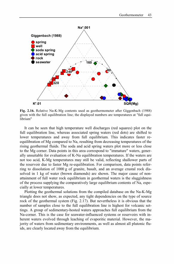
Geothermometer 43
K*.01 SQR(Mg)
Na*.001
80
160
240
320
Giggenbach (1988)
spring
well
soda spring
acid spring
rock
seawater
Fig. 2.16. Relative Na-K-Mg contents used as geothermometer after Giggenbach (1988)
given with the full equilibration line; the displayed numbers are temperatures at "full equi-
librium"
It can be seen that high temperature well discharges (red squares) plot on the
full equilibration line, whereas associated spring waters (red dots) are shifted to
lower temperatures and away from full equilibrium. This indicates faster re-
equilibration of Mg compared to Na, resulting from decreasing temperatures of the
rising geothermal fluids. The soda and acid spring waters plot more or less close
to the Mg corner. Data points in this area correspond to "immature" waters, gener-
ally unsuitable for evaluation of K-Na equilibration temperatures. If the waters are
not too acid, K-Mg temperatures may still be valid, reflecting shallower parts of
the reservoir due to faster Mg re-equilibration. For comparison, data points refer-
ring to dissolution of 1000 g of granite, basalt, and an average crustal rock dis-
solved in 1 kg of water (brown diamonds) are shown. The major cause of non-
attainment of full water rock equilibrium in geothermal waters is the sluggishness
of the process supplying the comparatively large equilibrium contents of Na, espe-
cially at lower temperatures.
Plotting the geothermal solutions from the compiled database on the Na-K-Mg
triangle does not show, as expected, any tight dependencies on the type of source
rock of the geothermal system (Fig. 2.17). But nevertheless it is obvious that the
number of samples close to the full equilibration line is highest for volcanic set-
tings. A group of sedimentary-hosted waters approaches full equilibrium from the
Na-corner. This is the case for seawater-influenced systems or reservoirs with in-
herent waters evolved through leaching of evaporitic material. However, the ma-
jority of waters from sedimentary environments, as well as almost all plutonic flu-
ids, are clearly located away from the equilibrium.
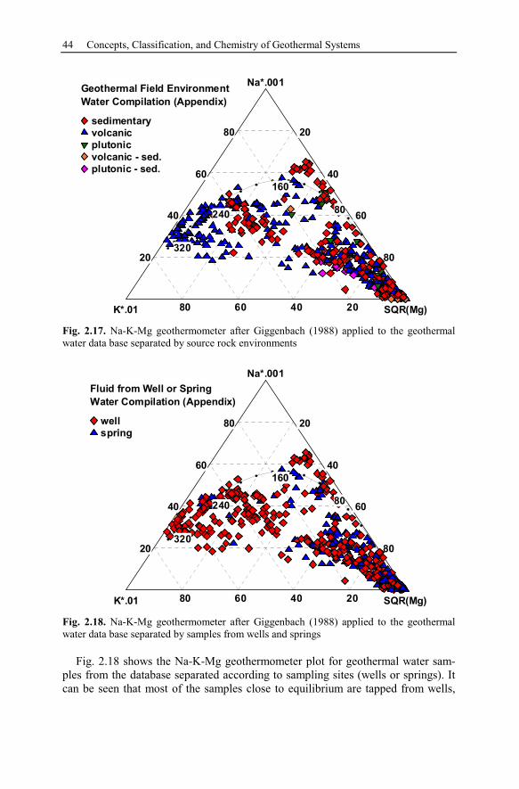
44 Concepts, Classification, and Chemistry of Geothermal Systems
80 60 40 20
20
40
60
80 20
40
60
80
K*.01 SQR(Mg)
Na*.001
80
160
240
320
Geothermal Field Environment
Water Compilation (Appendix)
sedimentary
volcanic
plutonic
volcanic - sed.
plutonic - sed.
Fig. 2.17. Na-K-Mg geothermometer after Giggenbach (1988) applied to the geothermal
water data base separated by source rock environments
80 60 40 20
20
40
60
80 20
40
60
80
K*.01 SQR(Mg)
Na*.001
80
160
240
320
Fluid from Well or Spring
Water Compilation (Appendix)
well
spring
Fig. 2.18. Na-K-Mg geothermometer after Giggenbach (1988) applied to the geothermal
water data base separated by samples from wells and springs
Fig. 2.18 shows the Na-K-Mg geothermometer plot for geothermal water sam-
ples from the database separated according to sampling sites (wells or springs). It
can be seen that most of the samples close to equilibrium are tapped from wells,
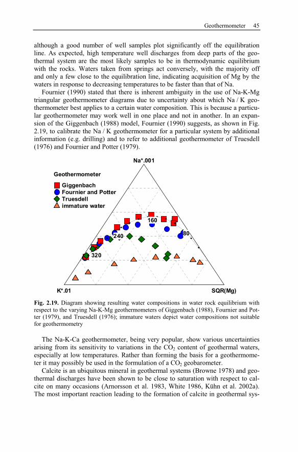
Geothermometer 45
although a good number of well samples plot significantly off the equilibration
line. As expected, high temperature well discharges from deep parts of the geo-
thermal system are the most likely samples to be in thermodynamic equilibrium
with the rocks. Waters taken from springs act conversely, with the majority off
and only a few close to the equilibration line, indicating acquisition of Mg by the
waters in response to decreasing temperatures to be faster than that of Na.
Fournier (1990) stated that there is inherent ambiguity in the use of Na-K-Mg
triangular geothermometer diagrams due to uncertainty about which Na / K geo-
thermometer best applies to a certain water composition. This is because a particu-
lar geothermometer may work well in one place and not in another. In an expan-
sion of the Giggenbach (1988) model, Fournier (1990) suggests, as shown in Fig.
2.19, to calibrate the Na / K geothermometer for a particular system by additional
information (e.g. drilling) and to refer to additional geothermometer of Truesdell
(1976) and Fournier and Potter (1979).
K*.01 SQR(Mg)
Na*.001
80
160
240
320
Geothermometer
Giggenbach
Fournier and Potter
Truesdell
immature water
Fig. 2.19. Diagram showing resulting water compositions in water rock equilibrium with
respect to the varying Na-K-Mg geothermometers of Giggenbach (1988), Fournier and Pot-
ter (1979), and Truesdell (1976); immature waters depict water compositions not suitable
for geothermometry
The Na-K-Ca geothermometer, being very popular, show various uncertainties
arising from its sensitivity to variations in the CO2 content of geothermal waters,
especially at low temperatures. Rather than forming the basis for a geothermome-
ter it may possibly be used in the formulation of a CO2 geobarometer.
Calcite is an ubiquitous mineral in geothermal systems (Browne 1978) and geo-
thermal discharges have been shown to be close to saturation with respect to cal-
cite on many occasions (Arnorsson et al. 1983, White 1986, Kühn et al. 2002a).
The most important reaction leading to the formation of calcite in geothermal sys-
46 Concepts, Classification, and Chemistry of Geothermal Systems
tems is the conversion of Ca-Al-silicates to calcite by CO2 [Eq. (2.3)]. Therefore
the system K-Ca is sensitive to variations of the CO2 fugacity (fCO2) following the
relationship published by Giggenbach (1988).
EQK-Ca = log (c2
K / cCa) = log fCO2 + 3.0 (2.29)
Before applying Eq. (2.29) to the estimation of the carbon dioxide activity in the
deeper parts of a geothermal reservoir the suitability of using the described geo-
barometer for certain geothermal waters should be checked. The maturity index
(MI) of the water, derived from the difference of the K-Mg and K-Na geother-
mometers, should be greater than 2.0.
MI = 0.315 EQK-Mg – EQK-Na (2.30)
3 Theory of Chemical Modeling
In order to deal with the complexity of natural systems simplified models are em-
ployed to illustrate the principal and regulatory factors controlling a chemical sys-
tem. Following the aphorism of Albert Einstein: "Everything should be made as
simple as possible, but not simpler", models need not to be completely realistic to
be useful (Stumm and Morgan 1996), but need to meet a successful balance be-
tween realism and practicality. Properly constructed, a model is neither too simpli-
fied that it is unrealistic nor too detailed that it cannot be readily evaluated and ap-
plied to the problem of interest (Bethke 1996). The results of a model have to be at
least partially observable or experimentally verifiable (Zhu and Anderson 2002).
Geochemical modeling theories are presented here in a sequence of increasing
complexity from geochemical equilibrium models to kinetic, reaction path, and fi-
nally coupled transport and reaction models. The description is far from complete
but provides the needs for the set up of reactive transport models of hydrothermal
systems as done within subsequent chapters. Extensive reviews of geochemical
models in general can be found in the literature (Appelo and Postma 1999, Bethke
1996, Melchior and Bassett 1990, Nordstrom and Ball 1984, Paschke and van der
Heijde 1996).
3.1 Geochemical Equilibrium
At the heart of any geochemical model is the thermodynamic equilibrium system,
which does not contain any spatial or temporal information. Hence, they are called
zero-dimensional models. In closed, open, or isolated systems, chemical reactions
tend to reach thermodynamic equilibrium, where all solute concentrations stabi-
lize. The concentrations at equilibrium are governed by thermodynamic principles.
At equilibrium, the potential energy, the Gibbs free energy, G, of the chemical
system is minimized. The Gibbs free energy is related to enthalpy H, representing
thermal energy, temperature, T, in Kelvin, and entropy, S, representing disorder or
randomness of a system.
G = H - TS (3.1)
The partial derivation of the Gibbs free energy with respect to the number of
moles of a substance, ni, corresponds to its chemical potential, µi.
Michael Kuhn: LNES 103, pp. 47–80, 2004.c© Springer-Verlag Berlin Heidelberg 2004
48 Theory of Chemical Modeling
i
i
G
n
∂= µ
∂(3.2)
Chemical potential is the driving force of chemical reactions and in turn depends
on the dimensionless activity, a, of the dissolved solution species via the following
equation, with the chemical potential at standard conditions (µ°) and the ideal gas
constant, R.
µi = µi° + RT ln a (3.3)
Activity calculation and the corresponding determination of mineral solubilities
are discussed in the following section.
3.1.1 Activity Calculations and Solubility of Minerals
Precipitation reactions might occur during the operation of a geothermal installa-
tion or due to diagenetic processes and are absolutely necessary for development
of ore deposits. They can be estimated using saturation indices calculated on the
basis of data from chemical analyses. The saturation index, SI, reflects the satura-
tion state of a solution with respect to a mineral phase. It is defined as:
eq
IAPSI log
K= (3.4)
In Eq. (3.4) the ion activity product, IAP, is the product of the "effective concen-
trations" of the dissolved species i, the so-called activities, ai (see below). It is
compared to the equilibrium constant, Keq, defined by the solubility product of the
mineral, which is the product of the equilibrium activities. If SI is positive, the
mineral is supersaturated and may precipitate. A mineral phase is in thermody-
namic equilibrium with a solution if the saturation index is equal to zero. How-
ever, fluids with saturation indices -0.2 SI 0.2 are also called saturated solu-
tions by Langmuir and Melchior (1985). Monnin and Ramboz (1996) specify
tighter limits of -0.05 SI 0.05. A negative saturation index indicates undersatu-
ration with respect to a mineral. The main task in calculating saturation indices is
to determine activities.
A concentration, mi, in mol kg-1
H2O is related to its activity (ai) using the di-
mensionless activity coefficient, γi, and the standard state (mi°), 1 mol kg-1
H2O:
ai = γi mi / mi° = γi mi (3.5)
The factor 1 / mi° is unity for all species and cancels for practical purposes (Appe-
lo and Postma 1999). In highly diluted solutions (i.e. for vanishing concentrations
of mi), the ionic interactions, reflected by γi, become negligibly small (γi =1). Then
the system behaves as an ideal solution. In this case, the activity of a species cor-
responds to its concentration in the solution. In non-ideal solutions there is elec-
trostatic interaction between ions and therefore γi ≠ 1. The Debye-Hückel equation
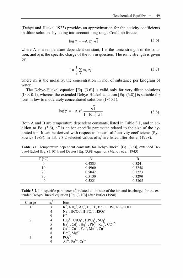
Geochemical Equilibrium 49
(Debye and Hückel 1923) provides an approximation for the activity coefficients
in dilute solutions by taking into account long-range Coulomb forces:
2
i ilog A z Iγ = − (3.6)
where A is a temperature dependent constant, I is the ionic strength of the solu-
tion, and zi is the specific charge of the ion in question. The ionic strength is given
by:
2
i ii
1I m z
2= (3.7)
where mi is the molality, the concentration in mol of substance per kilogram of
water.
The Debye-Hückel equation [Eq. (3.6)] is valid only for very dilute solutions
(I << 0.1), whereas the extended Debye-Hückel equation [Eq. (3.8)] is suitable for
ions in low to moderately concentrated solutions (I < 0.1).
2
i i 0
i
Ilog A z
1 B a I
γ = −+ (3.8)
Both A and B are temperature dependent constants, listed in Table 3.1, and in ad-
dition to Eq. (3.6), ai
0 is an ion-specific parameter related to the size of the hy-
drated ion. It can be derived with respect to "mean-salt" activity coefficients (Pyt-
kowicz 1983). In Table 3.2 selected values of ai
0 are listed after Butler (1998).
Table 3.1. Temperature dependent constants for Debye-Hückel [Eq. (3.6)], extended De-
bye-Hückel [Eq. (3.10)], and Davies [Eq. (3.9)] equation (Manov et al. 1943)
T [°C] A B
0 0.4883 0.3241
10 0.4960 0.3258
20 0.5042 0.3273
30 0.5130 0.3290
40 0.5221 0.3305
Table 3.2. Ion specific parameter ai
0, related to the size of the ion and its charge, for the ex-
tended Debye-Hückel equation [Eq. (3.10)] after Butler (1998)
Charge ai
0 Ions
1 3 K+, NH4
+, Ag
+, F
-, Cl
-, Br
-, I
-, HS
-, NO3
-, OH
-
4 Na+, HCO3
-, H2PO4
-, HSO3
-
9 H+
2 4 Hg2
2+, CrO4
2-, HPO4
2-, SO4
2-
5 Ba2+
, Cd2+
, Hg2+
, Pb2+
, Ra2+
, CO3
2-
6 Ca2+
, Cu2+
, Fe2+
, Mn2+
, Zn2+
8 Be2+
, Mg2+
3 4 PO4
3-
9 Al3+
, Fe3+
, Cr3+
50 Theory of Chemical Modeling
For brackish waters with ionic strength I > 0.1 the Davies equation [Eq. (3.9)]
is a better approximation of ion activity coefficients. It is valid up to I ≈ 0.5
(Stumm and Morgan 1996):
2
i i
Ilog A z 0.3I
1 I
γ = − −+
(3.9)
where A is the same constant from previous equations [Eqs. (3.6) and (3.8)] and
listed in Table 3.1. The Debye-Hückel, extended Debye-Hückel, and Davies equa-
tion are henceforth referred to as the Debye-Hückel theory.
For calculating species activities in solutions of higher ionic strength, an ion in-
teraction model was developed by Kenneth Pitzer and coworkers in the 1970s
(Pitzer 1973, 1975; Pitzer and Mayorga 1973, 1974; Pitzer and Kim 1974). This
semi-empirical approach combines the Debye-Hückel equation with additional
terms and describes the concentration dependence of the Gibbs energy for non-
ideal conditions. The free excess Gibbs energy, Gex
, indicating the difference be-
tween ideal and real Gibbs energy is written in the form of a virial equation (i.e. a
power series expansion):
ex
i j i j k i jki j i j k
w
Gf (I) m m B(I) m m m ...
w R T= + + Ψ + , (3.10)
with water mass wW, ionic strength I, and molality m of species i, j, and k. The
first term comprises the Debye-Hückel law, which accounts for the dependence on
the ionic strength and not on the individual parameters of the solution. It describes
the electrostatic far field interactions. The second virial coefficient, B, represents
the specific binary, near-field interactions between pairs of components i and j in
the solution. The corresponding ternary interactions between components i, j, and
k are described by the third virial coefficient, Ψ. For the limiting case of an ideally
diluted solution, the second and higher terms vanish, and the equation yields the
Debye-Hückel law. The series of virial coefficients can be extended to higher or-
ders but the first three virial coefficients are sufficient to describe solutions of high
salinity (Pitzer 1991). The activity coefficient is the derivative of Eq. (3.10) with
respect to mi and is calculated from
( ) ( )2
M M a M a M a c M c a M c aa c a
a a ' a a M M c a c aa a c a
ln z F m 2 B Z C m 2 m
m m z m m C′′<
γ = + + + Φ + Ψ
+ Ψ +(3.11)
for the cations and for anions from
( ) ( )2
X X c c X c X a X a c X a cc a c
c c c c X X c a c ac c c a
ln z F m 2 B Z C m 2 m
m m z m m C′ ′′<
γ = + + + Φ + Ψ
+ Ψ +(3.12)
Geochemical Equilibrium 51
Here, m is the molality of an ion, with indices M, c and c' for cations and X, a, and
a' for anions. The double sums c < c' and a < a' refer to all pairs of different cations
and anions. The function F contains an adapted form of the Debye-Hückel equa-
tion as well as the derivatives of the second virial coefficient with respect to the
ionic strength:
( ) c a cac a
c c ' cc a a a ac c a a
I 2F A ln 1 b I m m B
b1 b I
m m m m
φ
′ ′ ′′ ′< <
′= − + + ++
′ ′+ Φ + Φ
(3.13)
where ( )3/2
wA = 1400684 (D T)
φ ρ is the Debye-Hückel parameter, ρw water
density, and D the static dielectric constant of pure water. The coefficients B [Eq.
(3.11) and Eq. (3.12)] and B´ [Eq. (3.13)] are defined as:
( ) ( )( ) ( )
(0) (1) (2)
M X M X MX 1 M X 2
1 2(1) (2)
M X M X M X
B g I g I
g I g I
B .I I
= β + β α + β α
′ ′α α′ = β + β
(3.14)
For any salt containing a monovalent ion, values for α1 and α2 are α1 = 2 and
α2 = 0 (Pitzer 1973), while for 2-2 electrolytes and higher valence types the corre-
sponding values are α1 = 1.4 and α2 = 12.0 (Pitzer and Silvester 1976). The func-
tions g and g' are defined as:
( )
x 2
2 x 2
g(x) 2 1 (1 x)e / x
g (x) 2 1 1 x x 2 e / x
−
−
= − +
′ = − − + +(3.15)
where x=α√I. Actually, the coefficient C [Eq. (3.11) and Eq. (3.12)] depends on
the ionic strength, but there is only one experimental proof for this (Phutela and
Pitzer 1986). Therefore, C is defined according to Pitzer (1991) neglecting the in-
fluence of ionic strength:
( )MX MX M XC C 2 z z
φ= (3.16)
The coefficient Z for CMa and CcX in Eq. ((3.11) and Eq. ((3.12) is given by:
i ii
Z m z .= (3.17)
The thermodynamic properties of aqueous solutions containing a single salt
(i.e. binary systems) depend only on the interaction parameters β(0), β(1)
, β(2), and
Cφ which define the variables B and C. The parameters Φ and Ψ [Eq. (3.11) and
Eq. (3.12)] as well as Φ´ [Eq. (3.13)] correspond to aqueous mixtures of two salts
(i.e. ternary systems). The parameters Φ and Φ´ account for cation-cation and an-
52 Theory of Chemical Modeling
ion-anion interactions, the parameter Ψ for cation-cation-anion and anion-anion-
cation interactions.
The parameters Φi j and Φ´i j are defined by:
E E
i j i j i j i j i j(I) and (I)′ ′Φ = Θ + Θ Φ = Θ , (3.18)
where Θi j is the only adjustable parameter and is defined for each pair of cations
and each pair of anions. The terms E Θi j(I) and
E Θ´i j(I) account for electrostatic
mixing effects of asymmetrical (with respect to charge) cation-cation and anion-
anion pairs defined by Pitzer (1975). The values of E Θi j(I) and
E Θ´i j(I) depend
only on the charge of the ions and the ionic strength of the solution. They are
equal to zero if the corresponding cation or anion pairs i and j possess the same
charge. The parameters Ψi j k are introduced for different combinations of two
cations and one anion or two anions and one cation. Ψ is derived from data of so-
lutions containing two salts in the same way as Θi j.
A comprehensive compilation of Pitzer parameters applicable for the system
Na-K-Mg-Ca-Ba-Sr-Si-H-Cl-SO4-OH-HCO3-CO3-CO2-H2O from low to high
temperatures and salinities is given by Kühn et al. (2002b).
3.1.2 Comparison of Ion Activity Calculation Methods
An ideal model for calculating activity coefficients for geochemical or engineering
applications would have the following properties: (1) consistency with the laws of
thermodynamics; (2) compact mathematical form; (3) high accuracy over wide
ranges of temperature, pressure, and concentration; (4) applicability to systems in-
cluding most of the elements of the periodic table. Unfortunately, none of the cur-
rently existing models satisfies all of these requirements.
The Pitzer and the Debye-Hückel models represent different approaches to the
complex problem of calculating ion activities. Debye and Hückel described (1) the
solvent of an ionic solution as an ideal dielectric fluid without structure, and (2)
the solutes as uniform spherical ions with charges located at their centers. The far-
field Coulomb forces, which depend only on the ionic charge, cause each ion to be
surrounded by a fluctuating group of ions, the ionic sphere. Pitzer extends the De-
bye-Hückel theory and develops a semi-empirical model of complex solutions
which incorporates element-specific ion interactions, based on data of simpler bi-
nary and ternary systems containing one salt or two salts, respectively.
Due to its internal consistency and achievable calculation accuracy, the Pitzer
equations currently represent the most promising approach for calculating ion ac-
tivities in brines (Wolery and Jackson 1990).
As a typical example, Fig. 3.1 shows the solubility of gypsum in sodium chlo-
ride solutions at 25 °C, calculated according to both the Debye-Hückel theory
(here using the Davies equation) and the Pitzer model. Open and full circles repre-
sent data of Block and Waters (1968) and Marshall and Slusher (1966), respec-
tively. It is obvious that for concentrations larger than 0.5 mol kg-1
of sodium
chloride in the solution, only the Pitzer equations yield correct results. Therefore,
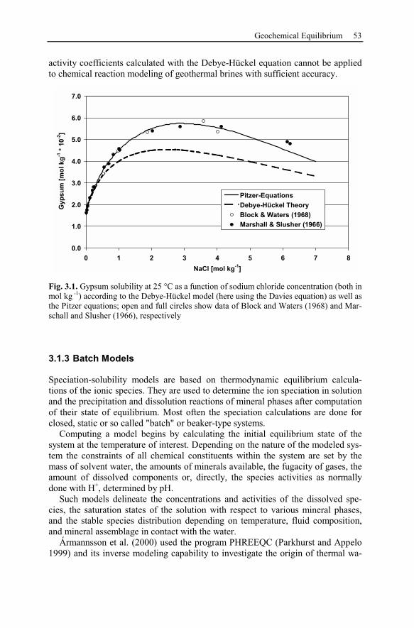
Geochemical Equilibrium 53
activity coefficients calculated with the Debye-Hückel equation cannot be applied
to chemical reaction modeling of geothermal brines with sufficient accuracy.
0.0
1.0
2.0
3.0
4.0
5.0
6.0
7.0
0 1 2 3 4 5 6 7 8
NaCl [mol kg-1
]
Gyp
su
m [
mo
l kg
-1 *
10
-2]
Pitzer-Equations
Debye-Hückel Theory
Block & Waters (1968)
Marshall & Slusher (1966)
Fig. 3.1. Gypsum solubility at 25 °C as a function of sodium chloride concentration (both in
mol kg -1
) according to the Debye-Hückel model (here using the Davies equation) as well as
the Pitzer equations; open and full circles show data of Block and Waters (1968) and Mar-
schall and Slusher (1966), respectively
3.1.3 Batch Models
Speciation-solubility models are based on thermodynamic equilibrium calcula-
tions of the ionic species. They are used to determine the ion speciation in solution
and the precipitation and dissolution reactions of mineral phases after computation
of their state of equilibrium. Most often the speciation calculations are done for
closed, static or so called "batch" or beaker-type systems.
Computing a model begins by calculating the initial equilibrium state of the
system at the temperature of interest. Depending on the nature of the modeled sys-
tem the constraints of all chemical constituents within the system are set by the
mass of solvent water, the amounts of minerals available, the fugacity of gases, the
amount of dissolved components or, directly, the species activities as normally
done with H+, determined by pH.
Such models delineate the concentrations and activities of the dissolved spe-
cies, the saturation states of the solution with respect to various mineral phases,
and the stable species distribution depending on temperature, fluid composition,
and mineral assemblage in contact with the water.
Ármannsson et al. (2000) used the program PHREEQC (Parkhurst and Appelo
1999) and its inverse modeling capability to investigate the origin of thermal wa-
54 Theory of Chemical Modeling
ters in the Lake Mývatn area of North Iceland. They divided the cold groundwater
and geothermal effluent of the area into six distinct groups according to origin and
geothermal influence. This division is based on stable isotope ratios, chemical
composition and geographical positions. Ármannsson et al. (2000) concluded that
the groundwater has apparently two basically separated origins; the local high
ground north of Lake Mývatn and the highlands far to the south. No traces of sea-
water are observed and the concentrations of conservative constituents suggest ex-
tensive water-rock interaction. The waters are variably affected by geothermal ac-
tivity. Simulating the composition of Krafla and Námafjall geothermal water by
titrating local groundwater with rock at 205°C and adding volcanic gas yield re-
sults in agreement with water analyses data.
3.2 Kinetic Models
For practical purposes, mineral reactions fall into three groups: (1) those in which
reaction rates may be so slow relative to the time period of interest that the reac-
tion can be ignored altogether, (2) those in which the rates are fast enough to
maintain equilibrium, and (3) the remaining reactions. Only those in the latter
group require a kinetic description.
Thermodynamic calculations deal only with the equilibrium state of geochemi-
cal systems (see preceding section), but due to the fact that concentrations of reac-
tants and products approach equilibrium depending on time and not instantane-
ously, kinetic processes may sometimes have to be taken into account in chemical
models. Calculations addressing chemical equilibrium are only possible if the
geochemical system remains essentially closed long enough for the reactions of
interest to approach equilibrium. For a more detailed study of the subject covered
in this section, the reader is referred to the comprehensive description of kinetic
theory in Earth sciences by Lasaga (1998).
Reaction rates vary tremendously. Some reactions are so fast that they can re-
sult in explosions, while others are so slow that geologic time scales are required
to measure their progress. General ranges of half life for several common types of
aqueous reactions are shown in Table 3.3.
Table 3.3. Approximate ranges of reaction half times for different types of reaction taken
from Langmuir and Mahoney (1984)
Type of Reaction Typical Half Life
Solute - solute Fraction of a second to minutes
Sorption - desorption Fraction of a second to days
Gas-solute Minutes to days
Crystalline solid - solute Hours to millions of years
Reactions involving more than one phase, for example minerals dissolving into
or precipitating from a solution, are called heterogeneous. The kinetics of hetero-
geneous reactions receive the most attention in reaction modeling, because of the
Kinetic Models 55
slow rates at which many minerals react and the resulting tendency of fluids, espe-
cially at low temperatures, to be in a state of non-equilibrium with the minerals in
contact.
Mineral dissolution reactions are often not in equilibrium because during the
time it takes to approach thermodynamic equilibrium the reservoir fluid has come
into contact with a different assemblage of minerals. When transport or other
agents of change are rapid compared to the reaction rate, disequilibrium prevails
and kinetic becomes an important factor in the estimation of concentrations. How-
ever, even when kinetics are important, equilibrium calculations may still be use-
ful to show where the system is heading in the long run.
Lasaga (1998) makes a useful distinction between "elementary" chemical reac-
tions, which occur as written at the molecular level, and "overall" reactions, which
describe a net change that involves several intermediate steps and takes place
along several competing, parallel pathways. Carbonate precipitation for example,
an important process during diagenesis, can be written as elementary reaction as:
Ca2+
+ CO3
2- ⇔ CaCO3 (3.19)
The rate at which molecules of CaCO3 are produced is directly proportional to the
probability that a Ca2+
ion will collide with a CO3
2- ion in solution. The appropri-
ate rate law in this case therefore is:
2 2
3
CaCO3
reac Ca CO
dmk m m
dt+ −= ⋅ ⋅ (3.20)
in which mi are the concentrations of each species i, and kreac is a linear rate con-
stant. In fact, for any elementary reaction, the rate is simply proportional to the
abundance of reactant species.
In contrast, the rates at which overall reactions occur are commonly non-linear
functions of concentration. Surface processes of particles, production of transient,
metastable species, or transport of dissolved material toward or away from the re-
action interface may influence the rates. As a result, rate laws may be quite com-
plex, reflecting a variety of inhibiting or enhancing processes. Keir (1980), for ex-
ample, has empirically determined that the rate of calcite dissolution (kreac) in
seawater follows the non-linear relationship
2 2
3
4.5
Ca CO
reac
eq
a a
k B 1K
+ −⋅= − (3.21)
in which B is an empirical constant that varies widely depending on the particular
system. It is especially a function of the reactive surface. Different approaches
have been used to model calcite dissolution in seawater by Sjöberg (1978),
Rickard and Sjöberg (1983), and Morse (1983). They can be generalized, as well
as Eq. (3.21), by the following empirical rate expression.
( )d
reac
Ak B 1 SI
V= − (3.22)
56 Theory of Chemical Modeling
where A is the reactive surface area, V is the volume of the solution, SI the satura-
tion index [Eq. (3.4)] reflecting the saturation state, and B and d are coefficients
depending on the composition of the solution and are obtained by curve fitting ob-
served rates.
The rate constant kreac [Eqs. (3.20) - (3.22)] can be related to the temperature by
the phenomenological Arrhenius equation.
AE / RT
reac 0k A e
−= ⋅ (3.23)
Here, A0 is the pre-exponential factor, EA an activation energy, R the gas constant,
and T the absolute temperature. The values of A0 and EA are determined for a
given reaction by measuring k at several temperatures.
Soler and Lasaga (1998) presented results of long-term numerical simulations
(> 1 Ma) of the formation of bauxite from granitic rocks. Within a one-
dimensional reactive transport model they used a kinetic approach to describe the
mineral dissolution and precipitation reactions. In agreement with numerous field
observations Soler and Lasaga (1998) determined the development of a typical
"bauxitic" profile consisting of an upper gibbsite-rich and a lower kaolinite-rich
zone. The simulations showed that the infiltrating solutions are closer to saturation
with respect to microcline than with respect to albite.
3.3 Reaction Pathways
Reaction path models simulate the successive reaction steps of a system in re-
sponse to the mass or energy flux. Within these kind of models, some temporal in-
formation is included in terms of reaction progress, but no spatial information is
contained. Once the initial equilibrium state of the system is known, the model can
trace a reaction path.
Chemical reaction path models have long been of use in the interpretation of
the chemical evolution of subsurface waters, often to determine the effect of
diagenetic reactions in a zone of interest. These models are constructions of hier-
archically arranged reaction pathways of batch reactions. The final solution com-
position or mineral assemblage of the preceding reaction step being the initial so-
lution or mineral assemblage of the proceeding step connects the batch reactions
with each other. This is based on the relative abundances of critical components
that serially dominate the reactions of the water-rock system (Saripalli et al. 2001).
Strictly speaking it is the course followed by the equilibrium system as it responds
to changes in composition or temperature. Reaction path models can be divided
into:
• Polythermal reaction models
• Titration models
• Systems open to external gas reservoirs
• Flow-through reaction path models
Reaction Pathways 57
3.3.1 Polythermal Reaction Models
The reaction path in polythermal models is characterized by the application of
varying temperatures or a temperature gradient to the system. Polythermal reac-
tion models are commonly applied to closed systems, as in studies of groundwater
geothermometry and interpretation of laboratory experiments. But there is no re-
striction for applying them also in open systems. If a fluid is, for example, sam-
pled at 300°C, but analyzed at room temperature, the thermal reaction path model
equilibrates the fluid at 25°C and then carries the closed system to the temperature
of the groundwater system or the experiment. One of these cases is the reconstruc-
tion of the pH under formation conditions. This is of importance with respect to
the investigation of hydrothermal reservoirs.
Reed and Spycher (1984) used chemical analyses and 25°C pH measurements
of geothermal waters from Iceland, Broadlands, and Sulphur Bank, hot spring wa-
ters from Jemez, Yellowstone and Blackfoot Reservoir to show that most of these
waters approach equilibrium with a subsurface mineral assemblage at a tempera-
ture close to measured temperatures. The in-situ pH values were recalculated and
by means of the mineral saturation indices they determined whether the distinct
waters are in equilibrium with their host rocks, the occurrence of probable mineral
assemblages, and the most likely temperature of equilibrium.
In a study of seawater-basalt reactions, Reed (1983) showed that in multicom-
ponent equilibrium calculations of tholeitic basalt with seawater at 300°C and sub-
sequent cooling to 25°C the resultant solutions can lead to ore deposition.
3.3.2 Titration Models
The titration model is the simplest open-system model. It is characterized by a re-
actant, which is gradually added to the solution in equilibrium. A titration can be
used to simulate (1) fluid mixing, where the reactant is a second aqueous solution
or (2) evaporation, in which the titrating substance, solvent water, is removed
from the system rather than added. In most cases the reactant will be (3) a mineral
undersaturated with respect to the initial solution. Adding an aliquot of the mineral
at each step the mineral will dissolve dependent on the fluid composition.
Thereby, the various titration models [(1)-(3)] may cause other minerals to be-
come saturated or even to precipitate or drive minerals that already exist in the
system to dissolve. Within the course of the reaction path of the titration model the
equilibrium system evolves until the fluid reaches saturation with the reactant or
the reactant is exhausted.
Titration models are applied to predict, for example, how rock will react with
its pore fluid. In that case, minerals that make up the rock are titrated into the for-
mation water. The solubility of most minerals in water is rather small, so the fluid
in such reaction path models is likely to become saturated after a small amount of
mineral has reacted.
Lu et al (1992) presented numerical results of skarn formation calculations us-
ing the program SOLVEQ (Reed 1982). An impure limestone (90% calcite and
58 Theory of Chemical Modeling
5% each of quartz and kaolinite) was titrated into a solution of a composition con-
strained by fluid inclusion investigations. The calculations demonstrated that a
complete sequence of skarn assemblages forms during progressive equilibration of
a very small amount of limestone with the infiltrating fluid.
3.3.3 System Open to External Gas Reservoirs
Many geochemical processes occur in which a fluid remains in contact with a
gaseous phase. The calculation of reaction path models open to external gas reser-
voirs assumes that gas species move to or from the solution in order to maintain a
specified fixed-fugacity in the reacting system. The gas, which could be the
Earth's atmosphere or a subsurface gas reservoir, buffers the system's chemistry.
By dissolving gas species from the buffer or exsolving gas into it, the fluid will, if
reaction proceeds slowly enough, maintain equilibrium with the buffer. The proc-
ess of gas exsolution might be triggered if a fluid boils.
Models of this type may be appropriate for describing weathering at Earth's sur-
face, reactions in soils, geochemical interactions in partially saturated rock forma-
tions, boiling in hydrothermal systems, and certain kinds of experimental configu-
rations. The gases most likely to be appropriately treated by this option are O2 and
CO2, with the possible oxidation reactions of pyrite (FeS2) to goethite (FeOOH)
4 FeS2 + 15 O2(aq) + 10 H2O ⇔ 4 FeOOH + 16 H+ + 8 SO4
2-(3.24)
or the exsolution of carbon dioxide accompanied by calcite precipitation.
Ca2+
+ 2 HCO3
- ⇔ CaCO3 + H2O + CO2(g) (3.25)
Saunders and Schoenly (1995) emphasized, using the program CHILLER
(Reed 1982, Spycher and Reed 1992), that a gold enriched fluid has been a princi-
pal factor in the genesis of Au-Ag ores. The numerical simulations showed that
boiling closely reproduces observed minerals and their relative abundances in bo-
nanza ores.
3.3.4 Flow-Through Reaction Path
Reaction between rock and groundwater moving through it is most appropriately
conceptualized by using a model configuration based on the assumption of local
equilibrium. Two major types of flow-through reaction path models can be used.
A fluid-centered flow-through system follows the evolution of a particular
packet of water as it flows through a medium, which could be a fractured or po-
rous material. Reactants are presumed to line the medium in homogeneous fashion
and interact with the fluid packet as it passes by. Alternatively, there may be no
reactants, but only a change in temperature or pressure. Within the course, secon-
dary mineral phases may form. As the packet moves on, it physically separates
from the masses of secondary phases produced. The result is that the transiently
Reaction Pathways 59
formed products do not have the opportunity to re-dissolve in that particular
packet of water.
A solid-centered flow-through system is fundamentally different. This reaction
path model focuses on the evolution of solids interacting with a mass of fluid,
which is either continuously or discretely recharged by a fresh supply of aqueous
solution of fixed composition. This system closely matches the scenario in many
flow-through interaction experiments.
Plumlee (1994) applied the reaction path model CHILLER to calculate changes
in the fluid chemistry and amounts of minerals precipitated from solution at each
of a series of steps along various chemical evolution paths. Around 150 reaction
paths were modeled to determine the sensitivity of probable ore deposition from
hydrothermal fluid compositions and corresponding temperatures as well as over-
lying meteoric groundwater compositions and temperatures, ambient pressure
conditions, the extent of boiling, and fluid reactions dependent on the mineral as-
semblages. The modeling results depict that epithermal ore grades and mineral
patterns are influenced to a great extent by boiling and fluid mixing in shallow
parts of hydrologic systems.
Plumlee et al. (1995a) used reaction path modeling to explain fluorite deposi-
tion mechanisms in the Illinois-Kentucky fluorspar district. They applied
CHILLER with temperatures, major cation and anion initials and amounts of dis-
solved gases based on fluid inclusion data. The investigated reaction path mecha-
nisms were simple cooling, reactions of the fluid with limestones, isothermal boil-
ing, mixing, and varying combinations of the enumerated processes. The results
indicate that quite acidic waters in the hydrothermal system are additionally rich in
fluorine, due to absorption of magmatic gases. The acidity of the geothermal fluids
led to extensive dissolution of the host rock limestone.
3.3.5 Reaction Path Models Applied to Hydrothermal Systems
Since a valid reaction model is a prerequisite for reactive transport simulation, the
first step in any case is to construct a successful reaction path model for the prob-
lem of interest.
Formation of Acidic Fluids in High Temperature Systems
Akaku et al. (2000) set up reaction path models for the high temperature hydro-
thermal reservoirs of Fushime and Kakkonda (Japan). Using the program
CHILLER they were able to explain the observed acidity of the discharged waters
without incorporating any acidic volatiles such as HCl or SO2.
Akaku et al. (2000) assumed a liquid formation fluid fully in equilibrium with
the alteration minerals in the rock. The geothermal water of Fushime originates
from seawater while the water in Kakkonda is believed to originate from meteoric
water. Due to a production-induced pressure decrease in the vicinity of the wells
the water begins to boil. Under consideration of heat transfer and in response to
the change of physical conditions due to the boiling process the reactions of the
60 Theory of Chemical Modeling
fluid versus a new state of equilibrium were investigated. The calculation results
emphasize that the acidity of the Fushime water results from sphalerite (ZnS) pre-
cipitation during boiling [Eq. (3.26)].
Zn2+
+ 2 Cl- + H2S ⇔ ZnS + 2 H
+ + 2 Cl
-(3.26)
The supply of acidity within the Kakkonda field is assumed to be due to the re-
actions of pyrite (FeS2) to magnetite (Fe3O4) [Eq. (3.27)] and the redox reaction of
hydrogen sulfide leading to hydrogen gas [Eq. (3.28)].
6 FeS2 + 12 H2O ⇔ 2 Fe3O4 + SO4
2- + 11 H2S + 2 H
+(3.27)
4 H2O + H2S ⇔ 4 H2 + SO4
2- + 2 H
+(3.28)
The fluid compositions calculated with the help of the reaction path models are in
agreement with the fluids discharged from the wells in Fushime as well as
Kakkonda.
Development of Ore Deposits Due to Vein Mineralization
In the Tongonan hydrothermal system (Philippines) the vein minerals sphalerite,
galena, chalcopyrite, pyrite, anhydrite, quartz, calcite, epidote-clinozoisite, and
chlorite are observed with specks of Au-Ag electrum. Balanque (2000) performed
calculations with CHILLER to investigate if either boiling or mixing is the better
precipitation mechanism to explain the mineral assemblage within the Tongonan
field.
Adiabatic boiling, with temperature changing from 300 to 100°C, lead to an
early precipitation sequence of gold with quartz followed by quartz, acanthite, and
chalcocite and finally late quartz, sphalerite, galena, acanthite, and bornite.
A steam-heated end member solution resulting from the boiling process has
been used for the mixing with a sample of the groundwater. This mixture pro-
duced the ore minerals acanthite, bornite, chalcocite, covellite, galena, pyrite, and
sphalerite accompanied by the gangue minerals anhydrite, Mg-chlorite, alunite,
kaolinite, muscovite, and quartz.
Balanque (2000) concluded that it might be possible, that a combination of the
boiling and mixture process may have led to the observed mineral assemblage.
The shortcomings of the simulations are the absence of some minerals within the
natural environment predicted by the program and the presence of other minerals
in the veins not predicted by the program.
Determination of a Reservoir Fluid's Origin
Gianelli and Grassi (2001) set up a reaction path model for Pantelleria Island (It-
aly) with which they confirmed, that the reservoir fluid is a mix of seawater, me-
teoric water, and volcanic gas. The code EQ3/6 (Wolery and Daveler 1992) has
been applied for the refinement of the conceptual model of the Pantelleria geo-
thermal system.
Simulation of Transport and Reaction 61
The system recharge is mainly of marine origin, which intrudes throughout the
island. The increasing temperature towards the center of the geothermal field leads
to the precipitation of anhydrite, quartz, and clay minerals resulting in decreased
amounts of Ca, Mg, and SO4. The seawater flows through fractures and is heated
to 300°C.
In the area of volcanic gas up flow the mixing results in increased quantities of
C and S. After reaction with trachyte the pH increases and the fluid reaches satura-
tion conditions with respect to albite, quartz, saponite, K-feldspar and muscovite,
in agreement with the natural hydrothermal mineral assemblages.
3.4 Simulation of Transport and Reaction
Reactive mass transport models contain both temporal and spatial information
about chemical reactions, a complexity that is desired for real world applications.
Basic processes that play significant roles in simultaneous and coupled simulation
of transport and reaction are fluid flow, heat transfer, solute transport, and chemi-
cal reactions. There are numerous books dealing with these diverse and complex
fields (e.g. Appelo and Postma 1999, Fitts 2002, Ingebritsen and Sanford 1998).
The essential elements of the theory will be incorporated here, with an emphasis
on the links to the other reaction topics within this book.
In this section, the equations, which are required to incorporate a velocity and
temperature field, or transport of species into the broad framework of chemical re-
actions, will be discussed. The discussion will include not only the equations that
govern flow, temperature, and transport itself, but also the feedback processes that
exist between these equations and the rates of chemical reactions.
In any treatment of fluid dynamics, the fundamental equations always start with
the three conservation equations: (1) the conservation of momentum, (2) conserva-
tion of mass – equation of continuity, and (3) conservation of energy.
3.4.1 Groundwater Flow
The primary coupling between groundwater flow, solute transport, and heat trans-
fer is through Darcy's law. The average linear groundwater flow velocity calcu-
lated by Darcy’s law is used to describe fluid flow in porous media. The Darcy ve-
locity is needed later to determine solute transport by advection, mechanical
dispersion, and heat transport by convection.
Darcy's Law
In 1856, a French hydraulic engineer named Henry Darcy published an equation
for flow through a porous medium that today bears his name. In designing a water
treatment system for the city of Dijon, Darcy found that no formulas existed for
determining the capacity of a sand filtration system. Consequently, Darcy per-
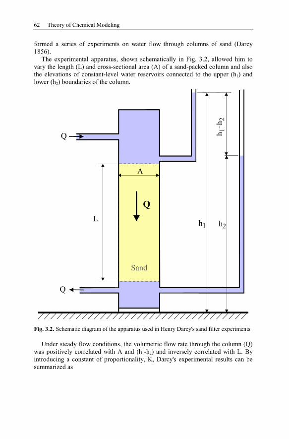
62 Theory of Chemical Modeling
formed a series of experiments on water flow through columns of sand (Darcy
1856).
The experimental apparatus, shown schematically in Fig. 3.2, allowed him to
vary the length (L) and cross-sectional area (A) of a sand-packed column and also
the elevations of constant-level water reservoirs connected to the upper (h1) and
lower (h2) boundaries of the column.
Fig. 3.2. Schematic diagram of the apparatus used in Henry Darcy's sand filter experiments
Under steady flow conditions, the volumetric flow rate through the column (Q)
was positively correlated with A and (h1-h2) and inversely correlated with L. By
introducing a constant of proportionality, K, Darcy's experimental results can be
summarized as
Simulation of Transport and Reaction 63
1 2h h
Q KA
L
−= (3.29)
The constant of proportionality (K) is called the hydraulic conductivity [L s-1
]. Eq.
(3.29) can be rewritten as:
1 2Q h h
K
A L
−= (3.30)
Writing Eq. (3.30) in differential form leads to the equation known as Darcy's law:
Q dhq K
A dl
= = − (3.31)
where q denotes the volumetric flow rate per unit area, called the specific dis-
charge or Darcy velocity. In Eq. (3.31), dh/dl is the dimensionless hydraulic gradi-
ent. The negative sign indicates that positive specific discharge (indicating direc-
tion of flow) corresponds to a negative hydraulic gradient. Thus, Darcy's Law
states that specific discharge in a porous medium is in the direction of decreasing
h and directly proportional to the hydraulic gradient. Although q has dimensions
of velocity [L s-1
], it is not the average groundwater velocity. This would only be
the case if the water could flow through all of the unit area A. However, in a sub-
surface medium only a fraction of the unit area is available for water flow. An aq-
uifer is composed by solid grains and voids in between, thus, the resulting average
velocity is higher than the specific discharge. The actual average linear fluid ve-
locity, v, is directly proportional to the specific discharge (q) and inversely propor-
tional to the effective porosity, ne.
e
qv
n
= (3.32)
The effective porosity is the porosity that is interconnected and available for flow.
The average linear velocity represents the mean flow velocity at which a conserva-
tive (non-reacting) solute would move through Darcy's experimental column as
shown in Fig. 3.2.
Subsequent laboratory-column experiments conducted using a variety of fluids
revealed that K expresses a combination of fluid and solid properties. The flow
rate is actually proportional to the specific weight of the fluid (ρ g) inversely pro-
portional to the dynamic viscosity of the fluid, µ, and proportional to a property of
the solid medium, k, which is called the intrinsic permeability. Thus
k gK
µ
ρ= (3.33)
where k has dimension of L2. Hubbert (1940, 1956) as well as Xu and Eckstein
(1997) revealed by theoretical considerations and experiments with glass beads or
64 Theory of Chemical Modeling
sands of uniform diameter, dm, that for granular porous media, q, K, and k are
proportional to dm
2. Hazen (1911) proposed the following empirical equation:
2
mK C d= ⋅ (3.34)
where K is hydraulic conductivity. If K is measured in cm s-1
and the constant C
with units of cm-1
s-1
, than C varies from about 40 to 150 for most sands.
Investigation of Darcy's Law indicates that it fails at sufficiently high volumet-
ric flow rates because above certain thresholds the kinetic energy of the fluid can-
not be neglected anymore and significant amounts of energy are lost to turbulence.
As a result, Darcy's Law over predicts the flow rate. Such flow rates are rare in the
subsurface but can occur in the direct vicinity of a well or in areas of cavernous
porosity. The upper limit for application of Darcy's Law is usually estimated on
the basis of the dimensionless Reynold's number,
qLRe
µ
ρ= (3.35)
where ρ is the fluid density, q the Darcy velocity, µ is the dynamic viscosity of the
fluid, and L is some characteristic length. In granular porous media, L is com-
monly related to the grain-size distribution. The transition from Darcian (laminar)
to non-Darcian (non-linear) flow appears to take place at Re ~ 5 and the transition
to turbulent flow occurs at Re ~ 100 (Bear 1979, Freeze and Cherry 1979).
The investigation of a possible lower limit for Darcian flow, done for fine-
grained materials, led to the suggestion that a threshold hydraulic gradient exists
below which flow does not take place (Swartzendruber 1962, Bolt and Groenevelt
1969). Although these findings are still under discussion, the phenomenon is of lit-
tle importance because the flow rates will be exceedingly small in any case.
Schildknecht and Schneider (1987) give a comprehensive description of the state
of the art of discussion about the validity of Darcy's Law under low hydraulic gra-
dients in sediments characterized by cohesion.
Driving Forces of Groundwater Flow
In hydrogeologic practice the driving force for groundwater flow is generally ex-
pressed in terms of a parameter called hydraulic head or simply head. This is the
same quantity indicated by h1 and h2 in Henry Darcy's laboratory manometers
(Fig. 3.2).
Intuitively, one might tend to think of groundwater as flowing from areas of
high pressure to areas of low pressure. But, considering the pressure distribution in
a static water column, expressed as:
P g z= ρ⋅ ⋅ (3.36)
where z is the depth below the water surface, this can be seen to not be the case.
Hubbert (1940) demonstrated that groundwater actually flows from areas of high
energy to areas of low energy.
Simulation of Transport and Reaction 65
Two fundamental forms of energy are of interest in this context: kinetic energy
and potential energy. Kinetic energy is associated with motion, but in a typical
groundwater environment the kinetic energy is negligibly small relative to the to-
tal potential energy (assumption for Darcian flow). Potential energy is associated
with the work required to move something from one place to another in a conser-
vative forces field. A conservative forces field is a field in which the work done in
moving from one point to another does not depend on the path taken. In the
groundwater context the most important conservative force fields are gravity and
pressure. The gravitational potential energy of a unit volume of liquid water is
ρf g z, where z is its height above an arbitrary datum and ρf g is its specific weight.
The pressure potential energy per unit volume is simply the pressure P, a force per
unit area. For a fluid with variable density (ρ not constant), flow is proportional to
the gradient in the quantity (P + ρf g z). For an incompressible fluid (ρ constant),
one can divide by the specific weight to obtain the hydraulic head, h:
f
Ph z
g
= +ρ
(3.37)
Both the pressure head (P / ρf g) and the elevation head (z) have units of length,
and the total hydraulic head (h) is equated to the water level observed in a ma-
nometer (Fig. 3.2) or well. In this case the driving force for groundwater flow is
the head gradient.
Intrinsic Permeability
Permeability is unquestionably the crucial hydrologic parameter. Unfortunately, it
is often a parameter very difficult to determine and apply in a meaningful fashion,
especially over the enormous space and time scales that apply in many geologic
problems. Permeability often appears to be a scale dependent property (Brace
1980, 1984; Clauser 1992).
The measured permeability of common geologic media varies by almost 16 or-
ders of magnitude, from values as low as 10-20
m2 in unaltered crystalline rock, in-
tact shales, and halite, to values as high as 10-7
m2 in well-sorted gravels (Table
3.4).
Permeability versus Porosity. The terms porosity (n) and permeability (k) are of-
ten used interchangeably by non-hydrogeologists. Although, this is a mistake,
there is a strong positive correlation between the two quantities in many porous
and fractured geologic media. For well-sorted, unconsolidated porous media, this
correlation is often expressed by the Kozeny-Carman equation (Carman 1956),
( )
3
22
0
nk
5s 1 n
=−
(3.38)
where s0 is the solid surface exposed to the fluid per unit volume of solid material
and the porosity. Solving the Navier-Stokes equations for a system of parallel cap-
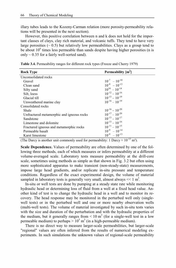
66 Theory of Chemical Modeling
illary tubes leads to the Kozeny-Carman relation (more porosity-permeability rela-
tions will be presented in the next section).
However, this positive correlation between n and k does not hold for the impor-
tant classes of clays, clay rich material, and volcanic tuffs. They tend to have very
large porosities (~ 0.5) but relatively low permeabilities. Clays as a group tend to
be about 106 times less permeable than sands despite having higher porosities (n is
only ~ 0.35 for a fairly well-sorted sand).
Table 3.4. Permeability ranges for different rock types (Freeze and Cherry 1979)
Rock Type Permeability [m2]
Unconsolidated rocks
Gravel 10-7
– 10-10
Clean sand 10-9
– 10-13
Silty sand 1010
– 10-14
Silt, loess 10-12
– 10-16
Glacial till 10-13
– 10-19
Unweathered marine clay 10-16
– 10-19
Consolidated rocks
Shale 10-16
– 10-20
Unfractured metamorphic and igneous rocks 10-17
– 10-20
Sandstone 10-13
– 10-17
Limestone and dolomite 10-13
– 10-16
Fractured igneous and metamorphic rocks 10-11
– 10-15
Permeable basalt 10-9
– 10-14
Karst limestone 10-9
– 10-13
(The Darcy is another unit commonly used for permeability: 1 Darcy 10-12
m²).
Scale Dependence. Values of permeability are often determined by one of the fol-
lowing three methods, each of which measures or infers permeability at a different
volume-averaged scale. Laboratory tests measure permeability at the drill-core
scale, sometimes using methods as simple as that shown in Fig. 3.2 but often using
more sophisticated apparatus to make transient (non-steady-state) measurements,
impose large head gradients, and/or replicate in-situ pressure and temperature
conditions. Regardless of the exact experimental design, the volume of material
sampled in laboratory tests is generally very small, almost always << 1 m3.
In-situ or well tests are done by pumping at a steady state rate while monitoring
hydraulic head or determining loss of fluid from a well at a fixed head value. An-
other kind of test is to change the hydraulic head in a well and to monitor its re-
covery. The head response may be monitored in the perturbed well only (single-
well tests) or in the perturbed well and one or more nearby observation wells
(multi-well tests). The volume of material investigated by such in-situ tests varies
with the size and duration of the perturbation and with the hydraulic properties of
the medium, but it generally ranges from < 10 m3 (for a single-well test in a low
permeable medium) to perhaps > 105 m
3 (in a high-permeable medium).
There is no direct way to measure larger-scale permeabilities, but larger-scale
"regional" values are often inferred from the results of numerical modeling ex-
periments. In such simulations the unknown values of regional-scale permeability
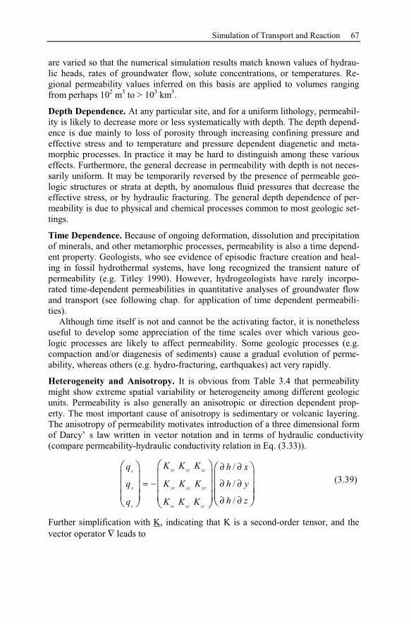
Simulation of Transport and Reaction 67
are varied so that the numerical simulation results match known values of hydrau-
lic heads, rates of groundwater flow, solute concentrations, or temperatures. Re-
gional permeability values inferred on this basis are applied to volumes ranging
from perhaps 102 m
3 to > 10
3 km
3.
Depth Dependence. At any particular site, and for a uniform lithology, permeabil-
ity is likely to decrease more or less systematically with depth. The depth depend-
ence is due mainly to loss of porosity through increasing confining pressure and
effective stress and to temperature and pressure dependent diagenetic and meta-
morphic processes. In practice it may be hard to distinguish among these various
effects. Furthermore, the general decrease in permeability with depth is not neces-
sarily uniform. It may be temporarily reversed by the presence of permeable geo-
logic structures or strata at depth, by anomalous fluid pressures that decrease the
effective stress, or by hydraulic fracturing. The general depth dependence of per-
meability is due to physical and chemical processes common to most geologic set-
tings.
Time Dependence. Because of ongoing deformation, dissolution and precipitation
of minerals, and other metamorphic processes, permeability is also a time depend-
ent property. Geologists, who see evidence of episodic fracture creation and heal-
ing in fossil hydrothermal systems, have long recognized the transient nature of
permeability (e.g. Titley 1990). However, hydrogeologists have rarely incorpo-
rated time-dependent permeabilities in quantitative analyses of groundwater flow
and transport (see following chap. for application of time dependent permeabili-
ties).
Although time itself is not and cannot be the activating factor, it is nonetheless
useful to develop some appreciation of the time scales over which various geo-
logic processes are likely to affect permeability. Some geologic processes (e.g.
compaction and/or diagenesis of sediments) cause a gradual evolution of perme-
ability, whereas others (e.g. hydro-fracturing, earthquakes) act very rapidly.
Heterogeneity and Anisotropy. It is obvious from Table 3.4 that permeability
might show extreme spatial variability or heterogeneity among different geologic
units. Permeability is also generally an anisotropic or direction dependent prop-
erty. The most important cause of anisotropy is sedimentary or volcanic layering.
The anisotropy of permeability motivates introduction of a three dimensional form
of Darcy’s law written in vector notation and in terms of hydraulic conductivity
(compare permeability-hydraulic conductivity relation in Eq. (3.33)).
/
/
/
xx xy xzx
y yx yy yz
z zx zy zz
K K Kq h x
q K K K h y
h zq K K K
∂ ∂
= − ∂ ∂
∂ ∂
(3.39)
Further simplification with K, indicating that K is a second-order tensor, and the
vector operator ∇ leads to
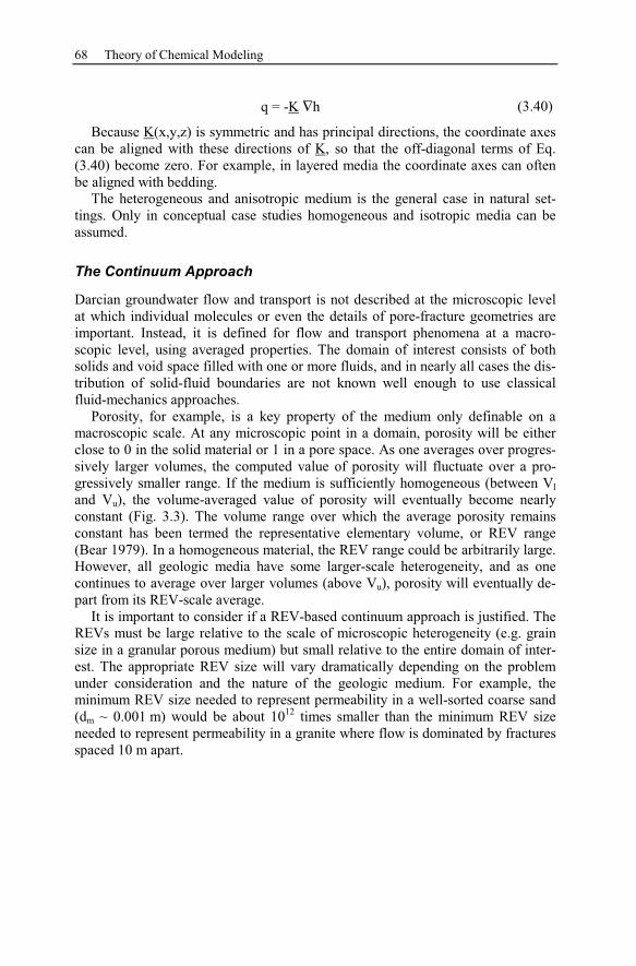
68 Theory of Chemical Modeling
q = -K ∇h (3.40)
Because K(x,y,z) is symmetric and has principal directions, the coordinate axes
can be aligned with these directions of K, so that the off-diagonal terms of Eq.
(3.40) become zero. For example, in layered media the coordinate axes can often
be aligned with bedding.
The heterogeneous and anisotropic medium is the general case in natural set-
tings. Only in conceptual case studies homogeneous and isotropic media can be
assumed.
The Continuum Approach
Darcian groundwater flow and transport is not described at the microscopic level
at which individual molecules or even the details of pore-fracture geometries are
important. Instead, it is defined for flow and transport phenomena at a macro-
scopic level, using averaged properties. The domain of interest consists of both
solids and void space filled with one or more fluids, and in nearly all cases the dis-
tribution of solid-fluid boundaries are not known well enough to use classical
fluid-mechanics approaches.
Porosity, for example, is a key property of the medium only definable on a
macroscopic scale. At any microscopic point in a domain, porosity will be either
close to 0 in the solid material or 1 in a pore space. As one averages over progres-
sively larger volumes, the computed value of porosity will fluctuate over a pro-
gressively smaller range. If the medium is sufficiently homogeneous (between Vl
and Vu), the volume-averaged value of porosity will eventually become nearly
constant (Fig. 3.3). The volume range over which the average porosity remains
constant has been termed the representative elementary volume, or REV range
(Bear 1979). In a homogeneous material, the REV range could be arbitrarily large.
However, all geologic media have some larger-scale heterogeneity, and as one
continues to average over larger volumes (above Vu), porosity will eventually de-
part from its REV-scale average.
It is important to consider if a REV-based continuum approach is justified. The
REVs must be large relative to the scale of microscopic heterogeneity (e.g. grain
size in a granular porous medium) but small relative to the entire domain of inter-
est. The appropriate REV size will vary dramatically depending on the problem
under consideration and the nature of the geologic medium. For example, the
minimum REV size needed to represent permeability in a well-sorted coarse sand
(dm ~ 0.001 m) would be about 1012
times smaller than the minimum REV size
needed to represent permeability in a granite where flow is dominated by fractures
spaced 10 m apart.
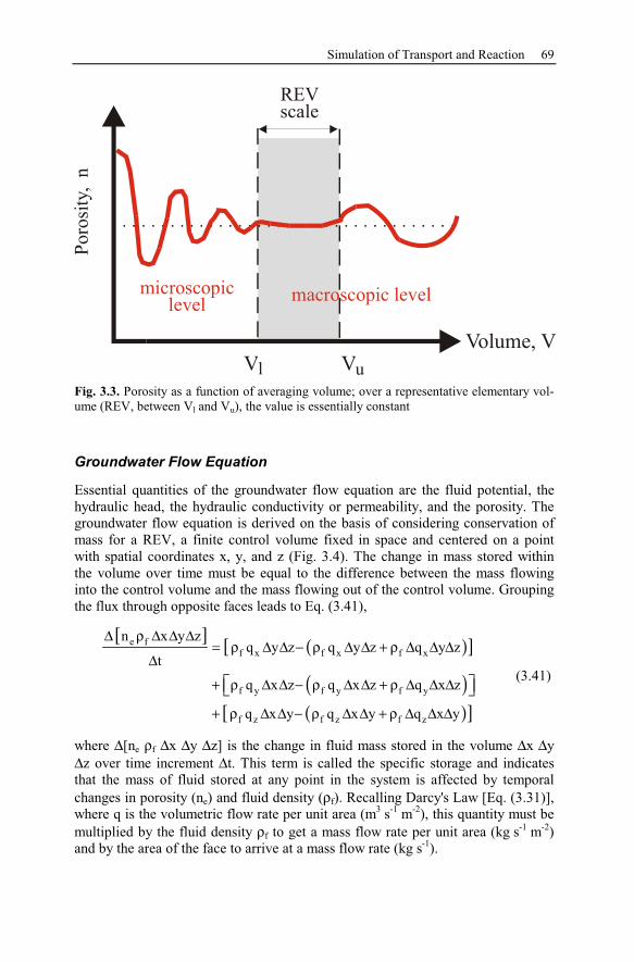
Simulation of Transport and Reaction 69
microscopic
levelmacroscopic level
REV
scale
Po
rosit
y,
n
Volume, V
Vl Vu
Fig. 3.3. Porosity as a function of averaging volume; over a representative elementary vol-
ume (REV, between Vl and Vu), the value is essentially constant
Groundwater Flow Equation
Essential quantities of the groundwater flow equation are the fluid potential, the
hydraulic head, the hydraulic conductivity or permeability, and the porosity. The
groundwater flow equation is derived on the basis of considering conservation of
mass for a REV, a finite control volume fixed in space and centered on a point
with spatial coordinates x, y, and z (Fig. 3.4). The change in mass stored within
the volume over time must be equal to the difference between the mass flowing
into the control volume and the mass flowing out of the control volume. Grouping
the flux through opposite faces leads to Eq. (3.41),
[ ] ( )[ ]
( )( )[ ]
e f
f x f x f x
f y f y f y
f z f z f z
n x y zq y z q y z q y z
t
q x z q x z q x z
q x y q x y q x y
∆ ρ ∆ ∆ ∆= ρ ∆ ∆ − ρ ∆ ∆ + ρ ∆ ∆ ∆
∆
+ ρ ∆ ∆ − ρ ∆ ∆ + ρ ∆ ∆ ∆
+ ρ ∆ ∆ − ρ ∆ ∆ + ρ ∆ ∆ ∆
(3.41)
where ∆[ne ρf ∆x ∆y ∆z] is the change in fluid mass stored in the volume ∆x ∆y
∆z over time increment ∆t. This term is called the specific storage and indicates
that the mass of fluid stored at any point in the system is affected by temporal
changes in porosity (ne) and fluid density (ρf). Recalling Darcy's Law [Eq. (3.31)],
where q is the volumetric flow rate per unit area (m3 s
-1 m
-2), this quantity must be
multiplied by the fluid density ρf to get a mass flow rate per unit area (kg s-1
m-2
)
and by the area of the face to arrive at a mass flow rate (kg s-1
).
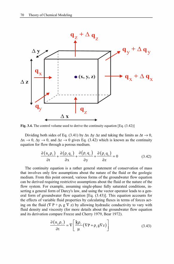
70 Theory of Chemical Modeling
(x, y, z)
∆ z x
y
zz
y
xq
q
qq + ∆
q + ∆
q + ∆
∆ y
∆ x
xq
yq
zq
Fig. 3.4. The control volume used to derive the continuity equation [Eq. (3.42)]
Dividing both sides of Eq. (3.41) by ∆x ∆y ∆z and taking the limits as ∆t → 0,
∆x → 0, ∆y → 0, and ∆z → 0 gives Eq. (3.42) which is known as the continuity
equation for flow through a porous medium.
( ) ( ) ( ) ( )f yf f x f zeqn q q
0
t x y z
∂ ρ∂ ρ ∂ ρ ∂ ρ+ + + =
∂ ∂ ∂ ∂(3.42)
The continuity equation is a rather general statement of conservation of mass
that involves only few assumptions about the nature of the fluid or the geologic
medium. From this point onward, various forms of the groundwater flow equation
can be derived requiring restrictive assumptions about the fluid or the nature of the
flow system. For example, assuming single-phase fully saturated conditions, in-
serting a general form of Darcy's law, and using the vector operator leads to a gen-
eral form of groundwater flow equation [Eq. (3.43)]. This equation accounts for
the effects of variable fluid properties by calculating fluxes in terms of forces act-
ing on the fluid (∇ P + ρf g ∇ z) by allowing hydraulic conductivity to vary with
fluid density and viscosity (for more details about the groundwater flow equation
and its derivation compare Freeze and Cherry 1979, Bear 1972).
( ) ( )f f
f
en
P g z
t
k∂ ρ ρ= ∇ ∇ + ρ ∇
∂ µ(3.43)
Simulation of Transport and Reaction 71
3.4.2 Solute Transport
The transport of solutes in groundwater is of particular importance for many geo-
logic processes like diagenesis, formation of ore deposits, or formation and disso-
lution of mineral phases. As is the case for groundwater flow, solute transport can
be described mathematically by combining principles of mass balance with ex-
pressions that relate the fluxes of solute to fundamental driving forces. Solutes
spread out by molecular diffusion, advection, and hydrodynamic dispersion.
Sources and sinks of solutes (e.g. chemical reactions) may also be incorporated
into solute-transport equations. If the solute-transport equations are coupled with
the groundwater flow equation as well as chemical reactions, they can be used to
quantify reactive-transport processes that occur in the subsurface.
Molecular Diffusion
Darcy's Law describes the flux of a fluid resulting from a gradient in fluid poten-
tial or hydraulic head [Eq. (3.31)]. An analogue situation exists for solute transport
due to diffusive flux as a result of a gradient in the chemical potential, or concen-
tration. This solute flux is directly proportional to the concentration gradient with
the coefficient of molecular diffusion as a proportionality factor. This is known as
Fick's first law and can be expressed for single-phase water as
d W
dCq D
dx
= − (3.44)
where qd is the diffusive flux, DW is the coefficient of molecular diffusion in free
or open water, C is the concentration of the molecule or ion, and x is the distance
along the direction of the concentration gradient. The physical process driving mo-
lecular diffusion is simply the random motion of ions in solution. Ions in a region
of higher concentration will eventually mix with ions in a region of lower concen-
tration (negative sign with always positive coefficient) to create an equal distribu-
tion in space. Table 3.5 lists molecular diffusion coefficients and ion radii for dif-
ferent cations and anions. These values show the general trend of decreasing value
with both increasing charge and decreasing ionic radius.
Eq. (3.44) expresses Fick's law in terms of DW for pure and open water. In the
subsurface, diffusion (Dm) occurs within a porous medium. The presence of a
solid phase restricts the area through which a solute can diffuse, and the tortuosity,
τ, of the flow path increases the distance over which the solute must travel to get
from one point to another. Tortuosity is dimensionless, always less than one, and
is a measure of how tortuous the flow path is. It can be described as the net
straight line length of flow divided by the average actual flow path. De Marsily
(1986) reported that tortuosity typically ranges from 0.7 (sands) to 0.1 (clays).
Bear (1972) stated a range of 0.56 < tortuosity < 0.8 for granular media. The effect
of tortuosity is that typical diffusion coefficients for geologic media range one to
two orders of magnitude lower, between 10-11
to 10-10
m2 s
-1, compared to open
water [Eq. (3.45)].
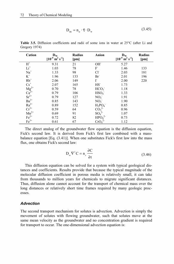
72 Theory of Chemical Modeling
Wm eD n D= ⋅ τ ⋅ (3.45)
Table 3.5. Diffusion coefficients and radii of some ions in water at 25°C (after Li and
Gregory 1974)
Cation DW
[10-9
m2 s
-1]
Radius
[pm]
Anion DW
[10-9
m2 s
-1]
Radius
[pm]
H+ 9.31 21 OH
- 5.27
Li+ 1.03 78 F
- 1.46 133
Na+ 1.33 98 Cl
- 2.03 181
K+ 1.96 133 Br
- 2.01 196
Rb+ 2.06 149 I
- 2.00 220
Cs+ 2.07 165 HS
- 1.73
Mg2+
0.70 78 HCO3
- 1.18
Ca2+
0.79 106 HSO4
- 1.33
Sr2+
0.79 127 NO2
- 1.91
Ba2+
0.85 143 NO3
- 1.90
Ra2+
0.89 152 H2PO4
- 0.85
Cr3+
0.59 64 CO3
2- 0.96
Mn2+
0.69 91 SO4
2- 1.07
Fe2+
0.72 82 HPO4
2- 0.73
Fe3+
0.61 67 CrO4
2- 1.12
The direct analog of the groundwater flow equation is the diffusion equation,
Fick's second law. It is derived from Fick's first law combined with a mass-
balance equation [Eq. (3.41)]. When one substitutes Fick's first law into the mass
flux, one obtains Fick's second law:
2
m e
CD C n
t
∂∇ =
∂(3.46)
This diffusion equation can be solved for a system with typical geological dis-
tances and coefficients. Results provide that because the typical magnitude of the
molecular diffusion coefficient in porous media is relatively small, it can take
from thousands to million years for chemicals to migrate significant distances.
Thus, diffusion alone cannot account for the transport of chemical mass over the
long distances or relatively short time frames required by many geologic proc-
esses.
Advection
The second transport mechanism for solutes is advection. Advection is simply the
movement of solutes with flowing groundwater, such that solutes move at the
same mean velocity as the groundwater and no concentration gradient is required
for transport to occur. The one-dimensional advection equation is:
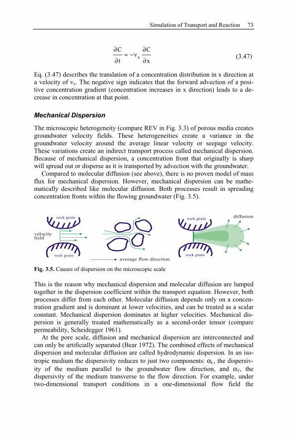
Simulation of Transport and Reaction 73
x
C Cv
t x
∂ ∂= −
∂ ∂(3.47)
Eq. (3.47) describes the translation of a concentration distribution in x direction at
a velocity of vx. The negative sign indicates that the forward advection of a posi-
tive concentration gradient (concentration increases in x direction) leads to a de-
crease in concentration at that point.
Mechanical Dispersion
The microscopic heterogeneity (compare REV in Fig. 3.3) of porous media creates
groundwater velocity fields. These heterogeneities create a variance in the
groundwater velocity around the average linear velocity or seepage velocity.
These variations create an indirect transport process called mechanical dispersion.
Because of mechanical dispersion, a concentration front that originally is sharp
will spread out or disperse as it is transported by advection with the groundwater.
Compared to molecular diffusion (see above), there is no proven model of mass
flux for mechanical dispersion. However, mechanical dispersion can be mathe-
matically described like molecular diffusion. Both processes result in spreading
concentration fronts within the flowing groundwater (Fig. 3.5).
average flow direction
velocity
field
diffusionrock grain
rock grainrock grain
rock grain
Fig. 3.5. Causes of dispersion on the microscopic scale
This is the reason why mechanical dispersion and molecular diffusion are lumped
together in the dispersion coefficient within the transport equation. However, both
processes differ from each other. Molecular diffusion depends only on a concen-
tration gradient and is dominant at lower velocities, and can be treated as a scalar
constant. Mechanical dispersion dominates at higher velocities. Mechanical dis-
persion is generally treated mathematically as a second-order tensor (compare
permeability, Scheidegger 1961).
At the pore scale, diffusion and mechanical dispersion are interconnected and
can only be artificially separated (Bear 1972). The combined effects of mechanical
dispersion and molecular diffusion are called hydrodynamic dispersion. In an iso-
tropic medium the dispersivity reduces to just two components: αL, the dispersiv-
ity of the medium parallel to the groundwater flow direction, and αT, the
dispersivity of the medium transverse to the flow direction. For example, under
two-dimensional transport conditions in a one-dimensional flow field the
74 Theory of Chemical Modeling
dimensional transport conditions in a one-dimensional flow field the dispersion
coefficient reduces to
W
xx L L x
e
DD D v
n
= = α + (3.48)
and
W
yy T T x
e
DD D v
n
= = α + (3.49)
where DL and DT are the longitudinal and transverse dispersion coefficients, re-
spectively. For a more thorough description see Bear (1972).
The dispersion coefficient as described above is normally applied in transport
simulations as macrodispersivity. Macrodispersivity is not a true physical property
of the porous medium, but is used as a fitting parameter to allow for simulation of
solute dispersion. The choice of this value depends of the scale of modeled trans-
port as shown by Gelhar et al. (1992) and the resolution of the specific simulation
model. For example, heterogeneity effects of the calculated area, which cannot be
reproduced in the model, are represented within the macrodispersion coefficient
(REV statement). Conversely, in homogenous media the dispersion coefficient is
dominated by the microdispersivity, which can be related to physical properties of
the porous media. Xu and Eckstein (1997) showed that the porosity and uniform-
ity of grain sizes are the two most important factors affecting the values of micro-
dispersivity. Microdispersivity is directly proportional to the uniformity coeffi-
cient and inversely proportional to porosity. Microdispersivity is also directly
proportional to the median grain size of homogenous clastic materials.
Microdispersivity is often used to describe transport in laboratory experiments,
whereas macrodispersivity is applied to field scale dispersion. Nevertheless, mi-
crodispersivity can be used to calculate macrodispersivity as shown by Gelhar and
Axness (1983). Microdispersivity sums up for a specific area to asymptotically
approach the value of macrodispersion in the limiting case.
Mass-Balance-Equation
The total solute concentration change at any given point is the sum of the fluxes of
advection, molecular diffusion, and mechanical dispersion. This total flux can be
substituted into a mass-balance equation to derive the solute transport equation.
Upon this substitution, a general case of the advective-dispersive equation is de-
rived:
( ) ( ) ( )e e s
n Cn D C n vC Q
t
∂ ρ∇ ρ ∇ − ∇ ρ + =
∂(3.50)
where D is the hydrodynamic dispersion tensor, C is the concentration in terms of
mass fraction, and Qs is a source (+) or sink (-) of solute. The solute source or sink
Simulation of Transport and Reaction 75
could be due to a net loss or gain of a fluid with a finite concentration or mass.
The source or sink term may incorporate any number of chemical reactions.
3.4.3 Heat Transport
General models of hydrothermal circulation in Earth's crust must accommodate a
large temperature range. Taking varying temperatures into account, the groundwa-
ter flow equation must be combined with heat transfer processes. Groundwater
flow and heat transfer can be described by a set of coupled equations expressing
mass and energy conservation.
Two basic types of heat transfer will be considered here. These are conductive
and convective (or advective) heat transfer, whereas radiation and thermal disper-
sion, the third and fourth basic types of heat transfer, respectively, are neglected.
Conductive heat transfer is the motion of heat through a stationary medium by vi-
bration of atoms, whereas convection of heat takes place by advective processes,
the transport of heat by a moving medium.
Conductive Heat Flux
Conductive heat transfer is governed by Fouriers law, which says that heat flux is
proportional to the temperature gradient, and the higher the gradient the greater
the amount of heat flow. Fourier's law of heat conduction is:
h e
dTq
dz
= −λ (3.51)
where qh is the heat flux, λe is the effective thermal conductivity of the medium
and T is temperature. Fourier's law is similar in form to Darcy's Law [Eq. (3.31)]
as well as Fick's law of diffusion [Eq. (3.44)]. Each of these laws describes a lin-
ear relation between a flux and a gradient in potential.
Whereas the hydraulic conductivity of crustal materials varies over approxi-
mately 16 orders of magnitude, the thermal conductivity of the upper crust gener-
ally varies by less than a factor of 5. Rock thermal conductivity can be up to 10
times greater than water thermal conductivity.
Especially at stagnant conditions, when heat transfer is due to conduction, it has
to be taken into account that the thermal conductivity of water is different from
that of rock. Therefore, the effective thermal conductivity, λe, is defined by:
( )e f r
n 1 nλ = λ + − λ (3.52)
where n is porosity, λf fluid conductivity, and λr conductivity of the rock. Al-
though thermal conductivity is treated here, and following, as a scalar, it has to be
kept in mind that it is a value which is generally an anisotropic or direction de-
pendent property like permeability or dispersivity (see above).
76 Theory of Chemical Modeling
Convective Heat Flux
Far more important in groundwater flow systems is convection, the transport of
heat by moving water. Two different kinds of convection exist: (1) forced convec-
tion and (2) free convection. In forced convection, the velocity of convective mo-
tion is independent on the temperatures in the fluid, it is part of the natural
groundwater flow system and therefore dependent on the hydraulic head (see
above). Thus, the groundwater movement forces heat energy transport. In free
convection, when only buoyancy effects in the fluid drive water velocities, these
are related to temperature change through the coefficient of thermal expansion
(see next section). In real and deep groundwater systems, there is a mixture of
both types of convection whereas in shallow aquifers, temperature and heat trans-
fer are negligible.
The simple expression of heat transport in forced convection is given by
e f p ( f )h eq T n C Tv= −λ ∇ + ρ (3.53)
Remembering that qh is heat flux (W m-2
), we see that Cp(w)T is the heat content
per unit mass of water, ρwCp(f)T is the heat content per unit volume of water,
ρwCp(f)Tv is the flux of heat (W m-2
) transported by velocity, v, per unit area.
Across the entire rock face this flux is reduced by the effective porosity, ne.
Conservation of Energy
The starting point for understanding temperature distribution in aquifers is conser-
vation of energy (energy inflow rate – energy outflow rate = change in energy
storage with time).
It should be remembered from earlier that the net flux of a vector across a test
volume is given by the divergence of the vector, so in the case of heat transport
the first two terms of the equation are simple. If no heat is advected, then Fouriers
law defines that the energy inflow rate minus energy outflow rate is given by
( )eh
q T−∇ = ∇ λ ∇ (3.54)
The net change in stored energy with time is simply
p
TC
t
∂ρ
∂(3.55)
so that conservation of energy is then
( )e p ( r )
TT C
t
∂∇ λ ∇ ρ
∂= (3.56)
But when heat is advected [Eq. (3.53)], the conduction-convection equation is
Simulation of Transport and Reaction 77
( )e f p ( f ) p ( r )e
TT n C Tv C
t
∂−∇ −λ ∇ + ρ = ρ
∂(3.57)
where the term C is used for the specific heat of water. Note that when the veloc-
ity is zero or perpendicular to the temperature gradient, this reduces to the simple
diffusion equation.
3.4.4 State of the Art of Hydrothermal Reactive Transport Simulation
The simulation of reactive transport requires that the equations described in the
previous sections be solved. This can be done either analytically or numerically.
Analytical solutions of transport processes of real-world problems do have a lim-
ited applicability, because heterogeneity and multidimensionality are reality and
additionally, the real world models do have complex constraints which cannot be
reflected in analytical solutions. But with the advent of computers, the numerical
solution of complex non-linear partial differential equations became possible.
However, the application of these techniques to model geothermal systems lagged
behind their application in groundwater or oil and gas reservoirs, because espe-
cially the coupling of mass and energy transport adds considerable complexity and
the economic driving force of the geothermal industry has been smaller.
Groundwater flow, heat transfer, and transport are commonly calculated based
on three different numerical solution techniques, finite differences, finite volumes,
or finite elements, each of which has particular advantages and disadvantages
when applied to the problem of interest. A description of these methods is beyond
the scope of this book, but such descriptions have been published in detail else-
where (e.g. Wang and Anderson 1982, Huyarkon and Pinder 1983, Fitts 2002).
Van der Lee and De Windt (2001) reviewed in general the present state of
simulation of geochemistry and hydrogeological systems. Their focus has been on
reactive transport processes in groundwater systems neglecting the effect of tem-
perature, which is of great importance for the investigation of geothermal reser-
voirs. O'Sullivan et al. (2001) presented the state of the art of geothermal reservoir
simulation and concluded that the use of computer modeling in planning and man-
agement has become standard practice during the last 10-15 years. They published
a comprehensive compilation of more than 100 computer modeled geothermal
fields worldwide. The restriction is that recent standard models of geothermal
fields only considers fluid flow and heat transfer. There are only a few cases in-
vestigating geochemical evolution and mineral recovery. Hence, O'Sullivan
(2001) predicts that the aim is still a fully coupled 3D mass and energy transport
model with detailed chemical interactions between aqueous fluids, gases and min-
eral assemblages, considering thermodynamic equilibrium as well as kinetic ef-
fects. Such kinds of models would provide a more realistic description of the cou-
pled physical and chemical processes inherent in geothermal reservoirs and more
generally in hydrothermal systems.
78 Theory of Chemical Modeling
At first it has to be stated that there already exists a variety of programs calcu-
lating fluid flow, heat transfer and mass transport or fluid flow, mass transport and
chemical reactions, but only a small number of codes are able to simulate all the
processes necessary for a comprehensive study of hydrothermal systems, which
are at least fluid flow, heat transfer, transport, and chemical reactions. Addition-
ally it is of importance that all the four processes have to be solved as intensively
coupled as necessary. Following is list and brief description of the capabilities of
available programs. All are specialized in particular fields with resulting inherent
advantages and disadvantages. At present there is no program favored over others:
• TOUGH2-Family (Pruess 1991): IFD (integral finite differences) code for
simulating flow and heat including 3 phases (water, vapor, organics) developed
for geothermal reservoir exploration and exploitation, nuclear waste dumping
sites, and hydrology in saturated and unsaturated media. Various modules for
reactive transport simulation are built up on the program by several authors:
• TOUGH / EWASG (Battistelli et al. 1997): The calculated system includes
water, salt (NaCl), and gas and additionally calculates dissolution and pre-
cipitation and resulting porosity-permeability changes.
• CHEM-TOUGH (White 1995): TOUGH2 extended for transport of reactive
species under consideration of Debye-Hückel activities within the chemical
calculations. The program supports a fixed and limited number of reactive
components (solutes and minerals) and calculates permeability changes due
to chemical reactions.
• TOUGHREACT (Xu and Pruess 2001): Generalized chemical module based
on Debye-Hückel activity coefficient calculations. Porosity-permeability in-
teractions are monitored but do not feed back on the flow.
• 3DHYDROGEOCHEM (Cheng and Yeh 1998): FE (finite elements) program
for saturated and unsaturated zone modeling including species transport and
chemical reactions (Debye-Hückel, equilibrium and kinetics) as well as micro-
biological processes. No porosity-permeability coupling or monitoring.
• RST2D (Raffensberger and Garven 1995a, 1995b): Program for coupled simu-
lation of fluid flow, heat transfer, transport, and chemistry (equilibrium and ki-
netics) with a fixed number of reacting components.
• FRACCHEM (Durst 2002): FE system for modeling coupled flow, heat, trans-
port, and reactions in fractured systems. Chemistry set up under special consid-
eration of and limited to the site Soultz-sous-Forets (France).
• SHEMAT (Bartels et al. 2003, Clauser 2003): FD (finite differences) simula-
tion code for fully coupled investigation of flow, heat, transport, and reactions.
The chemistry (equilibrium and kinetic) is applicable for dilute solutions (De-
bye-Hückel theory) to highly saline brines (Pitzer formalism). The chemical re-
actions are coupled on the flow via porosity-permeability relationships based
on varying methods. The number of reactive components is variable and can be
extended by the user.
Uncertainty, Usefulness, and Limitations of Models 79
3.5 Uncertainty, Usefulness, and Limitations of Models
The purpose of mathematical modeling is to develop a computer model that re-
flects essential features of the phenomenon considered or represents a real system.
Mathematical models are abstractions that replace objects, forces, and events by
expressions that contain variables, parameters, and constants (Krumbein and
Graybill 1965). However, one should remember that models provide only ap-
proximate solutions.
As the final product of the modeling process, a computer model includes all
simplifications and assumptions made at the previous steps, particularly at the
starting step when empirical data are conceptualized. Since there is always uncer-
tainty in empirical data, conceptual models may become a major source of error.
Dimensional analysis has proven to be efficient for testing conceptual models and
for identifying key physical processes. Errors in conceptualizing a problem are
easy to make but may be hard to discover. The modeler should begin work by in-
tegrating experimental results and field observations into the study. Having suc-
cessfully explained the experimental or field data, the modeler can extrapolate to
make predictions with greater confidence.
Zhu and Anderson (2002) stated that, on the one hand, a model generally must
be "verified", what means that it has to be checked if the computer code solves the
set of equations correctly and is free of serious bugs. Commonly, the user does not
have to bother with the "verification" of a program, because the developers nor-
mally "verify" distributed programs. On the other hand, it has to be "validated", if
the assumed conceptual model, which provides the basis for the set of equations
incorporated in the code, actually represents the natural processes of interest.
Here, the modeler has to ensure that the chosen computer code simulates the prob-
lem to be solved in a useful way. On the contrary, Konikow and Bredehoeft
(1992) argued convincingly that geochemical models couldn't be proven or vali-
dated but only tested and invalidated thus following the school of thought es-
poused by Popper (1959). However, Walter et al. (1994) stated that with increas-
ing model complexity either complete "verification" or "validation" may be
impossible, but above all, a model is valuable to get insight into complex proc-
esses. Zhu and Anderson (2002) follow this concurrent opinion and say that geo-
chemical and hydrogeological models are the best way to integrate and understand
data, concepts, and processes, which are coupled, but from different disciplines,
because reactive transport modeling is an interdisciplinary activity involving,
among others, numerical mathematics, geology, hydrology, physics, and chemis-
try. Anyway, the best way to avoid errors is to always critique your own results.
A geothermal system is never at steady state but undergoes various physical
and chemical processes. If a real geothermal process is slow, a quasi-static path
can approximate it. The evolution of a real system can then be modeled as a suc-
cession of equilibrium states (compare Reaction Path Models).
Calculating a geochemical or reactive transport model provides not only results
but also uncertainty about the accuracy of the results. Uncertainty, in fact, is an in-
tegral part of modeling that deserves as much attention as any other aspect of a
80 Theory of Chemical Modeling
study. The modeler, working with computer models, has to be aware of several
nuisance effects (Nitzsche et al. 2000):
• numerical problems of the code itself might occur,
• incomplete understanding of the physical and chemical phenomena,
• lack of precision of the geological and hydrogeological input data,
• missing data for a complete set up of a conceptual model,
• experimental uncertainties in the thermodynamic data.
The importance of a quantitative estimate of uncertainty within the thermody-
namic database is emphasized by (Nitzsche et al. 2000). They performed a Monte
Carlo analysis to show the impact of uncertainty in equilibrium on the elution and
break through of uranium from a sand column, which illustrates remediation prob-
lems of uranium mines. The variation of the thermodynamic input data, displaying
the effect of uncertainty within a database, and resulting transport predictions il-
lustrated that the complexity of a predictive model will be limited to the growing
uncertainty with the number input parameter affected by uncertainty. But unfortu-
nately, the Monte Carlo approach requires a very large number of repetitive calcu-
lations what is not feasible for 3D real world problems. This is one of the reasons
why uncertainties in modeling results are seldom provided. Hence, the modeler
should use his results to provide an impetus to determine more accurate thermo-
dynamic data, derive better chemical and physical models, and improve the under-
standing and the conceptual models of a site (Bethke 1996).
Reactive transport modeling can be extremely useful in understanding the spa-
tial and temporal distributions of solute concentrations and mineral assemblages in
the environment. The main target of reactive flow modeling is the simulation on a
real time scale with real spatial coordinates, but generally this goal is only par-
tially achievable. The limitations of reactive transport simulation are embedded in
the conceptualized set of equations used to best approximate the real situations.
But models provide a tool for critical analysis. They are a means to organize our
thinking, test ideas for their reasonableness, and indicate which are the sensitive
parameters. They point the way to further investigation and help to design new
experiments and to critically test hypotheses. Particularly surprising model outputs
often provide new insights otherwise inaccessible.
4 Specific Features of Coupled Fluid Flow and
Chemical Reaction
In many geologic processes, water-rock interactions are driven by continues sup-
ply of reactants provided by flowing groundwater. When water that carries dis-
solved chemical species moves through a permeable matrix or a network of frac-
tures a variety of chemical reactions can occur. Reactive transport processes are
important when there is a potential for fluid flow coexisting with spatial variations
in the thermodynamic states of the system. The resulting patterns of dissolution,
precipitation, and rock alteration depend on the reaction kinetics and the rate at
which reactants in solution can be delivered to the reaction site by advection and
diffusion.
Five fundamental end-member types of reactive transport environments, setting
up the basis for the discussion of specific features of coupled flow and reaction
within this chapter, are distinguished in the following:
• "Flow across mineralogical boundaries" describes the equilibrium approach of
a water body moving into a geological environment with a different assemblage
of minerals (time independent).
• "Moving reaction fronts" are characterized by a mineralogical boundary propa-
gating in flow direction because of the time dependent depletion of the origi-
nally reacting mineral.
• "Reactions within thermal gradients" are caused by variations in temperature
across a region where the mineral assemblage might otherwise be constant.
• "Mixing zone environments" exhibit reactions due to variation in aqueous com-
position. The mixture of two different waters, both in equilibrium with respect
to the same mineral assemblage, may result in a mixing disequilibrium due to
the nonlinearity of chemical reactions.
• "Local flow enhancement due to faults" depicts fluid transport through other-
wise impermeable layers. This focusing of fluid flow may lead to or accelerate
precipitation or dissolution of minerals.
These five distinct systems lead to flow induced spatial reaction patterns. How-
ever, it is most likely to encounter overlapping end-member types within natural
environments. Specific examples, presented here, are preferential flow path devel-
opment and diagenesis due to thermal convection. Before proceeding to discuss
individual processes, the key for understanding the majority of reactive transport
phenomena, changes of permeability due to reactive porosity increase or decrease,
is investigated. The porosity-permeability relationship represents the basis for the
coupling of flow and transport.
Michael Kuhn: LNES 103, pp. 81–116, 2004.c© Springer-Verlag Berlin Heidelberg 2004
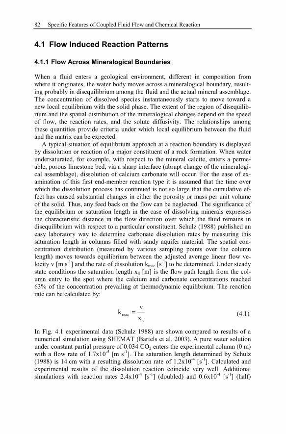
82 Specific Features of Coupled Fluid Flow and Chemical Reaction
4.1 Flow Induced Reaction Patterns
4.1.1 Flow Across Mineralogical Boundaries
When a fluid enters a geological environment, different in composition from
where it originates, the water body moves across a mineralogical boundary, result-
ing probably in disequilibrium among the fluid and the actual mineral assemblage.
The concentration of dissolved species instantaneously starts to move toward a
new local equilibrium with the solid phase. The extent of the region of disequilib-
rium and the spatial distribution of the mineralogical changes depend on the speed
of flow, the reaction rates, and the solute diffusivity. The relationships among
these quantities provide criteria under which local equilibrium between the fluid
and the matrix can be expected.
A typical situation of equilibrium approach at a reaction boundary is displayed
by dissolution or reaction of a major constituent of a rock formation. When water
undersaturated, for example, with respect to the mineral calcite, enters a perme-
able, porous limestone bed, via a sharp interface (abrupt change of the mineralogi-
cal assemblage), dissolution of calcium carbonate will occur. For the ease of ex-
amination of this first end-member reaction type it is assumed that the time over
which the dissolution process has continued is not so large that the cumulative ef-
fect has caused substantial changes in either the porosity or mass per unit volume
of the solid. Thus, any feed back on the flow can be neglected. The significance of
the equilibrium or saturation length in the case of dissolving minerals expresses
the characteristic distance in the flow direction over which the fluid remains in
disequilibrium with respect to a particular constituent. Schulz (1988) published an
easy laboratory way to determine carbonate dissolution rates by measuring this
saturation length in columns filled with sandy aquifer material. The spatial con-
centration distribution (measured by various sampling points over the column
length) moves towards equilibrium between the adjusted average linear flow ve-
locity v [m s-1
] and the rate of dissolution kreac [s-1
] to be determined. Under steady
state conditions the saturation length xS [m] is the flow path length from the col-
umn entry to the spot where the calcium and carbonate concentrations reached
63% of the concentration prevailing at thermodynamic equilibrium. The reaction
rate can be calculated by:
S
reac
vk
x
= (4.1)
In Fig. 4.1 experimental data (Schulz 1988) are shown compared to results of a
numerical simulation using SHEMAT (Bartels et al. 2003). A pure water solution
under constant partial pressure of 0.034 CO2 enters the experimental column (0 m)
with a flow rate of 1.7x10⁻⁵
[m s-1
]. The saturation length determined by Schulz
(1988) is 14 cm with a resulting dissolution rate of 1.2x10⁻⁴
[s-1
]. Calculated and
experimental results of the dissolution reaction coincide very well. Additional
simulations with reaction rates 2.4x10⁻⁴
[s-1
] (doubled) and 0.6x10⁻⁴
[s-1
] (half)
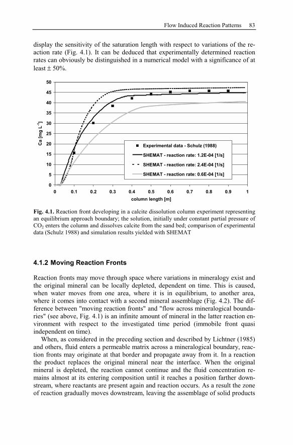
Flow Induced Reaction Patterns 83
display the sensitivity of the saturation length with respect to variations of the re-
action rate (Fig. 4.1). It can be deduced that experimentally determined reaction
rates can obviously be distinguished in a numerical model with a significance of at
least ± 50%.
0
5
10
15
20
25
30
35
40
45
50
0 0.1 0.2 0.3 0.4 0.5 0.6 0.7 0.8 0.9 1
column length [m]
Ca [
mg
L-1
]
Experimental data - Schulz (1988)
SHEMAT - reaction rate: 1.2E-04 [1/s]
SHEMAT - reaction rate: 2.4E-04 [1/s]
SHEMAT - reaction rate: 0.6E-04 [1/s]
Fig. 4.1. Reaction front developing in a calcite dissolution column experiment representing
an equilibrium approach boundary; the solution, initially under constant partial pressure of
CO2 enters the column and dissolves calcite from the sand bed; comparison of experimental
data (Schulz 1988) and simulation results yielded with SHEMAT
4.1.2 Moving Reaction Fronts
Reaction fronts may move through space where variations in mineralogy exist and
the original mineral can be locally depleted, dependent on time. This is caused,
when water moves from one area, where it is in equilibrium, to another area,
where it comes into contact with a second mineral assemblage (Fig. 4.2). The dif-
ference between "moving reaction fronts" and "flow across mineralogical bounda-
ries" (see above, Fig. 4.1) is an infinite amount of mineral in the latter reaction en-
vironment with respect to the investigated time period (immobile front quasi
independent on time).
When, as considered in the preceding section and described by Lichtner (1985)
and others, fluid enters a permeable matrix across a mineralogical boundary, reac-
tion fronts may originate at that border and propagate away from it. In a reaction
the product replaces the original mineral near the interface. When the original
mineral is depleted, the reaction cannot continue and the fluid concentration re-
mains almost at its entering composition until it reaches a position farther down-
stream, where reactants are present again and reaction occurs. As a result the zone
of reaction gradually moves downstream, leaving the assemblage of solid products
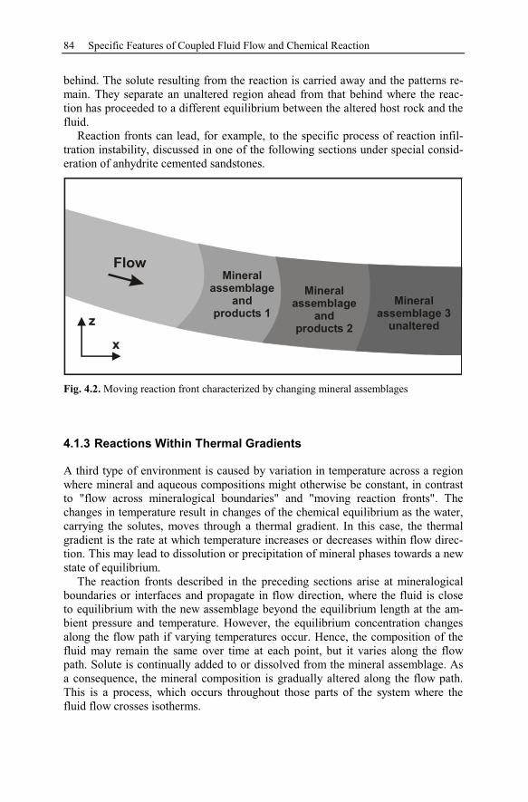
84 Specific Features of Coupled Fluid Flow and Chemical Reaction
behind. The solute resulting from the reaction is carried away and the patterns re-
main. They separate an unaltered region ahead from that behind where the reac-
tion has proceeded to a different equilibrium between the altered host rock and the
fluid.
Reaction fronts can lead, for example, to the specific process of reaction infil-
tration instability, discussed in one of the following sections under special consid-
eration of anhydrite cemented sandstones.
Mineral
assemblage
and
products 1
Mineral
assemblage
and
products 2
Mineral
assemblage 3
unaltered
Fig. 4.2. Moving reaction front characterized by changing mineral assemblages
4.1.3 Reactions Within Thermal Gradients
A third type of environment is caused by variation in temperature across a region
where mineral and aqueous compositions might otherwise be constant, in contrast
to "flow across mineralogical boundaries" and "moving reaction fronts". The
changes in temperature result in changes of the chemical equilibrium as the water,
carrying the solutes, moves through a thermal gradient. In this case, the thermal
gradient is the rate at which temperature increases or decreases within flow direc-
tion. This may lead to dissolution or precipitation of mineral phases towards a new
state of equilibrium.
The reaction fronts described in the preceding sections arise at mineralogical
boundaries or interfaces and propagate in flow direction, where the fluid is close
to equilibrium with the new assemblage beyond the equilibrium length at the am-
bient pressure and temperature. However, the equilibrium concentration changes
along the flow path if varying temperatures occur. Hence, the composition of the
fluid may remain the same over time at each point, but it varies along the flow
path. Solute is continually added to or dissolved from the mineral assemblage. As
a consequence, the mineral composition is gradually altered along the flow path.
This is a process, which occurs throughout those parts of the system where the
fluid flow crosses isotherms.
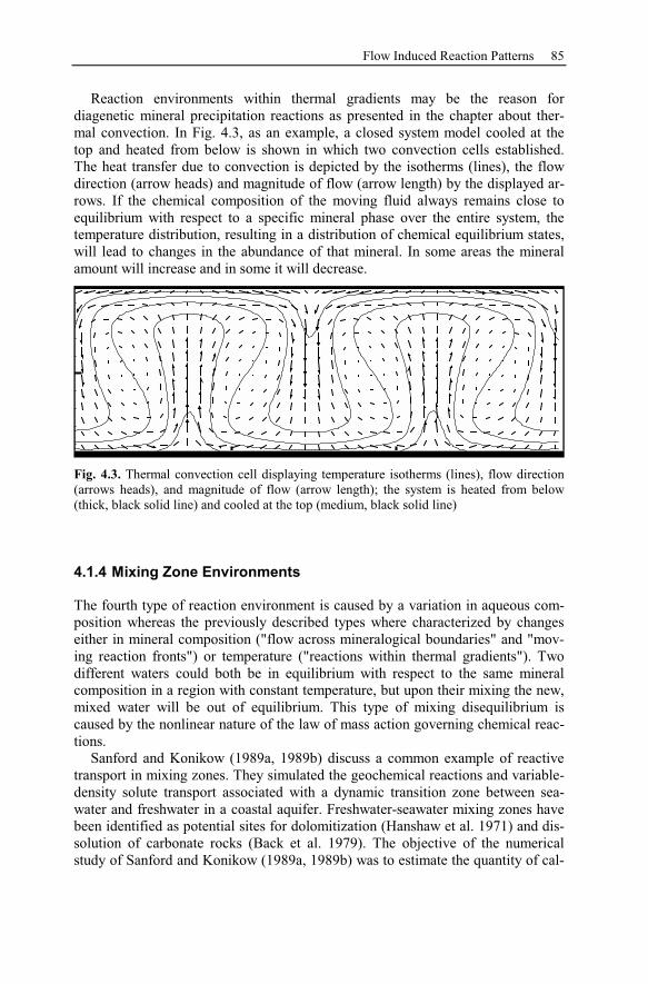
Flow Induced Reaction Patterns 85
Reaction environments within thermal gradients may be the reason for
diagenetic mineral precipitation reactions as presented in the chapter about ther-
mal convection. In Fig. 4.3, as an example, a closed system model cooled at the
top and heated from below is shown in which two convection cells established.
The heat transfer due to convection is depicted by the isotherms (lines), the flow
direction (arrow heads) and magnitude of flow (arrow length) by the displayed ar-
rows. If the chemical composition of the moving fluid always remains close to
equilibrium with respect to a specific mineral phase over the entire system, the
temperature distribution, resulting in a distribution of chemical equilibrium states,
will lead to changes in the abundance of that mineral. In some areas the mineral
amount will increase and in some it will decrease.
Fig. 4.3. Thermal convection cell displaying temperature isotherms (lines), flow direction
(arrows heads), and magnitude of flow (arrow length); the system is heated from below
(thick, black solid line) and cooled at the top (medium, black solid line)
4.1.4 Mixing Zone Environments
The fourth type of reaction environment is caused by a variation in aqueous com-
position whereas the previously described types where characterized by changes
either in mineral composition ("flow across mineralogical boundaries" and "mov-
ing reaction fronts") or temperature ("reactions within thermal gradients"). Two
different waters could both be in equilibrium with respect to the same mineral
composition in a region with constant temperature, but upon their mixing the new,
mixed water will be out of equilibrium. This type of mixing disequilibrium is
caused by the nonlinear nature of the law of mass action governing chemical reac-
tions.
Sanford and Konikow (1989a, 1989b) discuss a common example of reactive
transport in mixing zones. They simulated the geochemical reactions and variable-
density solute transport associated with a dynamic transition zone between sea-
water and freshwater in a coastal aquifer. Freshwater-seawater mixing zones have
been identified as potential sites for dolomitization (Hanshaw et al. 1971) and dis-
solution of carbonate rocks (Back et al. 1979). The objective of the numerical
study of Sanford and Konikow (1989a, 1989b) was to estimate the quantity of cal-
86 Specific Features of Coupled Fluid Flow and Chemical Reaction
cite dissolution under typical hydrodynamic and geochemical conditions to assess
changes of the rock properties porosity and permeability, because resulting per-
meability changes in turn affect the flow system. The results illustrate the use of a
fully coupled reaction-transport model for analyzing diagenetic processes. They
indicate that porosity development within the mixing zone would not be evenly
distributed. Porosity develops on the freshwater side of the transition zone. Poros-
ity also develops faster at the base or toe of the mixing zone and at its top, in the
discharge area at the coastline. Including a permeability-porosity feedback al-
lowed the flow system to respond to dissolution over time. As porosity is en-
hanced on the freshwater side of the mixing zone, the resulting permeability en-
hancement causes the transition zone to migrate landward over time.
4.1.5 Local Flow Enhancement due to Faults
The characteristic feature of the fifth reaction environment is caused by particular
hydrodynamic conditions. Fault and fracture zones provide pathways for fluid
transport through otherwise impermeable layers. In already permeable zones,
planes or surfaces of high permeability attract focusing of fluid flow. This local
flow enhancement in turn may accelerate the process of deposition or dissolution
that becomes part of the geological record. Deposition leads to veins of minerali-
zation and dissolution to enlargement of the interstices and possibly increased
flow rates.
When a fracture traverses a relatively impermeable layer between two more
permeable layers, it opens a fluid pathway that allows for mixing of interstitial flu-
ids from one region to the other and provides the opportunity for chemical reac-
tions between the entering fluid and its new environment. This type of reaction
system is investigated later as one opportunity of mineral deposition within a deep
seated aquifer located in Northern Germany (Chap. 5).
4.2 Porosity and Permeability (Reduction) Models
Permeability is unquestionably the crucial hydrologic parameter. Unfortunately, it
is often a very difficult parameter to determine and apply in a meaningful fashion.
This is especially due to its enormous variation over space and time in natural sys-
tems.
In many geologic problems permeability must be regarded as a time-dependent
parameter (see above), being increased or decreased over time by mineral dissolu-
tion and precipitation, by changes in effective stress that result in consolidation or
hydraulic fracturing, and by thermoelastic effects. Permeability changes due to
mineral reactions will be discussed in detail in the following. Permeability reduc-
tion due to consolidation effects where studied, for example, by Kühn et al.
(2002c) for a geothermal reservoir under exploitation and by Gambolatti et al.
(1996) for utilization of subsurface fluids in general.
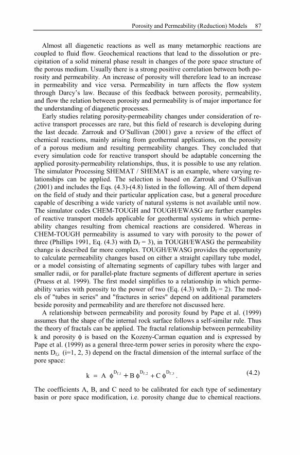
Porosity and Permeability (Reduction) Models 87
Almost all diagenetic reactions as well as many metamorphic reactions are
coupled to fluid flow. Geochemical reactions that lead to the dissolution or pre-
cipitation of a solid mineral phase result in changes of the pore space structure of
the porous medium. Usually there is a strong positive correlation between both po-
rosity and permeability. An increase of porosity will therefore lead to an increase
in permeability and vice versa. Permeability in turn affects the flow system
through Darcy’s law. Because of this feedback between porosity, permeability,
and flow the relation between porosity and permeability is of major importance for
the understanding of diagenetic processes.
Early studies relating porosity-permeability changes under consideration of re-
active transport processes are rare, but this field of research is developing during
the last decade. Zarrouk and O’Sullivan (2001) gave a review of the effect of
chemical reactions, mainly arising from geothermal applications, on the porosity
of a porous medium and resulting permeability changes. They concluded that
every simulation code for reactive transport should be adaptable concerning the
applied porosity-permeability relationships, thus, it is possible to use any relation.
The simulator Processing SHEMAT / SHEMAT is an example, where varying re-
lationships can be applied. The selection is based on Zarrouk and O’Sullivan
(2001) and includes the Eqs. (4.3)-(4.8) listed in the following. All of them depend
on the field of study and their particular application case, but a general procedure
capable of describing a wide variety of natural systems is not available until now.
The simulator codes CHEM-TOUGH and TOUGH/EWASG are further examples
of reactive transport models applicable for geothermal systems in which perme-
ability changes resulting from chemical reactions are considered. Whereas in
CHEM-TOUGH permeability is assumed to vary with porosity to the power of
three (Phillips 1991, Eq. (4.3) with Df = 3), in TOUGH/EWASG the permeability
change is described far more complex. TOUGH/EWASG provides the opportunity
to calculate permeability changes based on either a straight capillary tube model,
or a model consisting of alternating segments of capillary tubes with larger and
smaller radii, or for parallel-plate fracture segments of different aperture in series
(Pruess et al. 1999). The first model simplifies to a relationship in which perme-
ability varies with porosity to the power of two (Eq. (4.3) with Df = 2). The mod-
els of "tubes in series" and "fractures in series" depend on additional parameters
beside porosity and permeability and are therefore not discussed here.
A relationship between permeability and porosity found by Pape et al. (1999)
assumes that the shape of the internal rock surface follows a self-similar rule. Thus
the theory of fractals can be applied. The fractal relationship between permeability
k and porosity φ is based on the Kozeny-Carman equation and is expressed by
Pape et al. (1999) as a general three-term power series in porosity where the expo-
nents Df,i (i=1, 2, 3) depend on the fractal dimension of the internal surface of the
pore space:
f ,1 f ,2 f ,3D D D
k A B C= φ φ + φ+ .(4.2)
The coefficients A, B, and C need to be calibrated for each type of sedimentary
basin or pore space modification, i.e. porosity change due to chemical reactions.
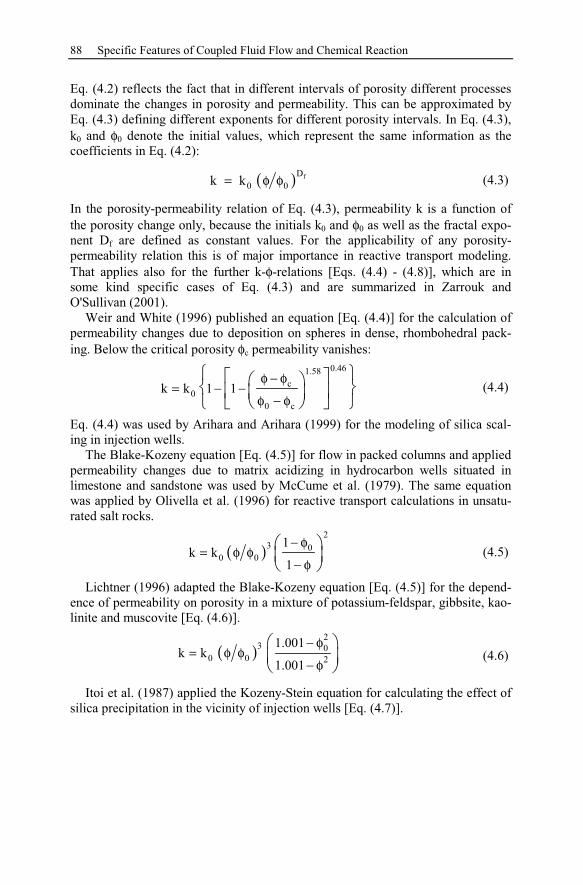
88 Specific Features of Coupled Fluid Flow and Chemical Reaction
Eq. (4.2) reflects the fact that in different intervals of porosity different processes
dominate the changes in porosity and permeability. This can be approximated by
Eq. (4.3) defining different exponents for different porosity intervals. In Eq. (4.3),
k0 and φ0 denote the initial values, which represent the same information as the
coefficients in Eq. (4.2):
( ) fD
0 0k k= φ φ (4.3)
In the porosity-permeability relation of Eq. (4.3), permeability k is a function of
the porosity change only, because the initials k0 and φ0 as well as the fractal expo-
nent Df are defined as constant values. For the applicability of any porosity-
permeability relation this is of major importance in reactive transport modeling.
That applies also for the further k-φ-relations [Eqs. (4.4) - (4.8)], which are in
some kind specific cases of Eq. (4.3) and are summarized in Zarrouk and
O'Sullivan (2001).
Weir and White (1996) published an equation [Eq. (4.4)] for the calculation of
permeability changes due to deposition on spheres in dense, rhombohedral pack-
ing. Below the critical porosity φc permeability vanishes:
0.461.58
c
0
0 c
k k 1 1φ − φ
= − −φ − φ
(4.4)
Eq. (4.4) was used by Arihara and Arihara (1999) for the modeling of silica scal-
ing in injection wells.
The Blake-Kozeny equation [Eq. (4.5)] for flow in packed columns and applied
permeability changes due to matrix acidizing in hydrocarbon wells situated in
limestone and sandstone was used by McCume et al. (1979). The same equation
was applied by Olivella et al. (1996) for reactive transport calculations in unsatu-
rated salt rocks.
( )2
3 0
0 0
1k k
1
− φ= φ φ
− φ(4.5)
Lichtner (1996) adapted the Blake-Kozeny equation [Eq. (4.5)] for the depend-
ence of permeability on porosity in a mixture of potassium-feldspar, gibbsite, kao-
linite and muscovite [Eq. (4.6)].
( )2
3 0
0 0 2
1.001k k
1.001
− φ= φ φ
− φ(4.6)
Itoi et al. (1987) applied the Kozeny-Stein equation for calculating the effect of
silica precipitation in the vicinity of injection wells [Eq. (4.7)].
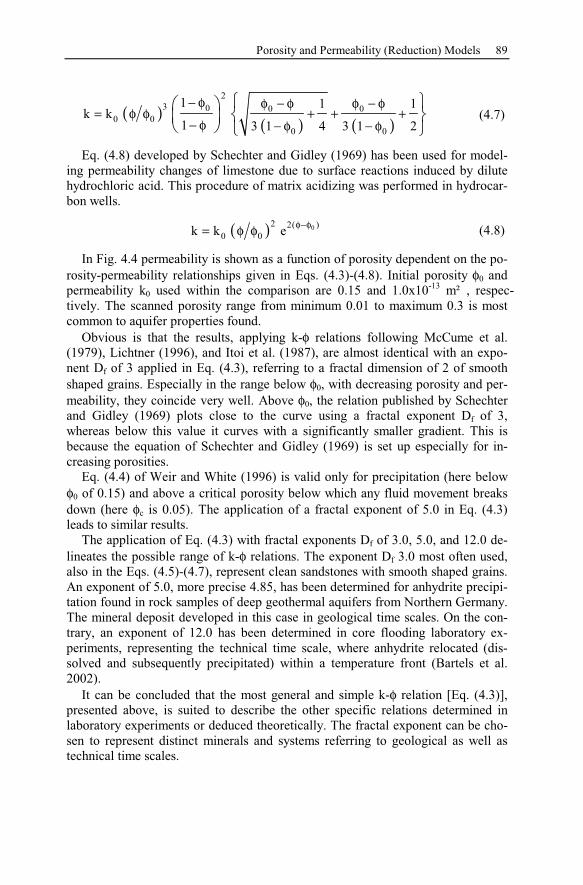
Porosity and Permeability (Reduction) Models 89
( )( ) ( )
2
3 0 0 0
0 0
0 0
1 1 1k k
1 3 1 4 3 1 2
− φ φ − φ φ − φ+ + += φ φ
− φ − φ − φ(4.7)
Eq. (4.8) developed by Schechter and Gidley (1969) has been used for model-
ing permeability changes of limestone due to surface reactions induced by dilute
hydrochloric acid. This procedure of matrix acidizing was performed in hydrocar-
bon wells.
( ) 02 2( )
0 0k k e
φ−φ= φ φ (4.8)
In Fig. 4.4 permeability is shown as a function of porosity dependent on the po-
rosity-permeability relationships given in Eqs. (4.3)-(4.8). Initial porosity φ0 and
permeability k0 used within the comparison are 0.15 and 1.0x10⁻¹³
m², respec-
tively. The scanned porosity range from minimum 0.01 to maximum 0.3 is most
common to aquifer properties found.
Obvious is that the results, applying k-φ relations following McCume et al.
(1979), Lichtner (1996), and Itoi et al. (1987), are almost identical with an expo-
nent Df of 3 applied in Eq. (4.3), referring to a fractal dimension of 2 of smooth
shaped grains. Especially in the range below φ0, with decreasing porosity and per-
meability, they coincide very well. Above φ0, the relation published by Schechter
and Gidley (1969) plots close to the curve using a fractal exponent Df of 3,
whereas below this value it curves with a significantly smaller gradient. This is
because the equation of Schechter and Gidley (1969) is set up especially for in-
creasing porosities.
Eq. (4.4) of Weir and White (1996) is valid only for precipitation (here below
φ0 of 0.15) and above a critical porosity below which any fluid movement breaks
down (here φc is 0.05). The application of a fractal exponent of 5.0 in Eq. (4.3)
leads to similar results.
The application of Eq. (4.3) with fractal exponents Df of 3.0, 5.0, and 12.0 de-
lineates the possible range of k-φ relations. The exponent Df 3.0 most often used,
also in the Eqs. (4.5)-(4.7), represent clean sandstones with smooth shaped grains.
An exponent of 5.0, more precise 4.85, has been determined for anhydrite precipi-
tation found in rock samples of deep geothermal aquifers from Northern Germany.
The mineral deposit developed in this case in geological time scales. On the con-
trary, an exponent of 12.0 has been determined in core flooding laboratory ex-
periments, representing the technical time scale, where anhydrite relocated (dis-
solved and subsequently precipitated) within a temperature front (Bartels et al.
2002).
It can be concluded that the most general and simple k-φ relation [Eq. (4.3)],
presented above, is suited to describe the other specific relations determined in
laboratory experiments or deduced theoretically. The fractal exponent can be cho-
sen to represent distinct minerals and systems referring to geological as well as
technical time scales.
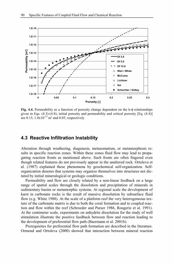
90 Specific Features of Coupled Fluid Flow and Chemical Reaction
1.E-18
1.E-17
1.E-16
1.E-15
1.E-14
1.E-13
1.E-12
1.E-11
1.E-10
0 0.05 0.1 0.15 0.2 0.25 0.3
Porosity [-]
Perm
eab
ilit
y [
m²]
Df 3.0
Df 5.0
Df 12.0
Weir / White
McCume
Lichtner
Itoi
Schechter / Gidley
Fig. 4.4. Permeability as a function of porosity change dependent on the k-φ relationships
given in Eqs. (4.3)-(4.8); initial porosity and permeability and critical porosity [Eq. (4.4)]
are 0.15, 1.0x10⁻¹³
m² and 0.05, respectively
4.3 Reactive Infiltration Instability
Alteration through weathering, diagenesis, metasomatism, or metamorphosis re-
sults in specific reaction zones. Within these zones fluid flow may lead to propa-
gating reaction fronts as mentioned above. Such fronts are often fingered even
though related features do not previously appear in the unaltered rock. Ortoleva et
al. (1987) explained these phenomena by geochemical self-organization. Self-
organization denotes that systems may organize themselves into structures not dic-
tated by initial mineralogical or geologic conditions.
Permeability and flow are closely related by a non-linear feedback on a large
range of spatial scales through the dissolution and precipitation of minerals in
sedimentary basins or metamorphic systems. At regional scale the development of
karst in carbonate rocks is the result of massive dissolution by subsurface fluid
flow (e.g. White 1988). At the scale of a platform reef the very heterogeneous tex-
ture of the carbonate matrix is due to both the coral formation and to coupled reac-
tion and flow within the reef (Schroeder and Purser 1986, Rougerie et al. 1991).
At the centimeter scale, experiments on anhydrite dissolution for the study of well
stimulation illustrate the positive feedback between flow and reaction leading to
the development of preferential flow path (Baermann et al. 2001b).
Prerequisites for preferential flow path formation are described in the literature.
Ormond and Ortoleva (2000) showed that interaction between mineral reaction
Reactive Infiltration Instability 91
and mass transport in rocks can lead to reaction front instability. The development
of channel-like voids occurs if the characteristic Peclet and Damköhler numbers,
describing the reactive flow system, fall in a specific range.
4.3.1 Peclet and Damköhler Number
Flow coupled with transport of solutes generated by mineral dissolution can lead
to self-organized enhancement of the heterogeneity in the rock (Ortoleva 1994). If
the initial rock texture is perfectly uniform, the resulting reaction front will remain
planar while advancing down stream with time. However, if the rock texture is ini-
tially even slightly non-uniform, the resulting enhancement of the permeability
will be uneven and a fingering reaction front may form (Wei and Ortoleva 1990).
Fluid flows preferentially in regions with higher permeability. If the fluid is un-
dersaturated with regard to a specific mineral phase, mineral dissolution occurs.
Locally restricted, dissolution is faster in regions of higher permeability. The in-
crease in porosity leads to an increase in permeability. The permeability increase
in turn causes higher flow rate of undersaturated solution. Due to that positive
feedback loop, preferential flow paths arise.
Compensation of the concentration gradient via dispersion or diffusion counter-
acts the formation, because the undersaturation, which is the driving force of the
process, decreases (Ormond and Ortoleva 2000).
Whether such preferential flow paths may develop, can be determined by
evaluating the dimensionless Peclet (Pe) and Damköhler (Da) number.
L m
v l v lPe
D v D
⋅ ⋅= =
α ⋅ +(4.9)
In Eq. (4.9) v is the mean flow velocity, l the characteristic length (in this case the
thickness of the system or cross section drained), and D the dispersion coefficient
composed of the dispersivity αL and the diffusion coefficient Dm. Additionally in
Eq. (4.10) kreac is the kinetic coefficient of the mineral reaction (compare Chap. 3).
reack l
Da
v
⋅= (4.10)
The relation between dispersion and advection determines the preferential flow
path length. If dispersion evens out the concentration within the flow path, the
growth of the channel stops. The Peclet number [Eq. (4.9)] expresses the relation
between advection and dispersion. With Peclet numbers above 10 preferential
flow paths develop and if Peclet numbers are infinite preferential flow paths grow
infinitely long.
The Damköhler number [Eq. (4.10)] describes the relation between the time a
chemical reaction requires to reach equilibrium and the time the fluid needs to
flow through the characteristic length. Where Da < 1 the reaction rate cannot keep
up with the advection term and local disequilibrium results. Planar reaction fronts
92 Specific Features of Coupled Fluid Flow and Chemical Reaction
result from Da < 10-2
(Steefel and Lasaga 1990). When Da >> 1 the rate of chemi-
cal reaction is much larger than the rate at which the solute is transported by flow
and the solution remains close to equilibrium. If the kinetics of the chemical disso-
lution and precipitation reactions are neglected, which means thermodynamic
equilibrium is assumed, the Damköhler number becomes infinite.
4.3.2 Example of Preferential Flow Path Development
Kühn and Stöfen (2001) and Kühn (2003) demonstrated in numerical experiments
the development of preferential flow paths. The simulations are based on labora-
tory experiments to determine mineral dissolution rates in anhydrite (CaSO4) ce-
mented sandstone samples (Baermann et al. 2000b). Both the numerical and labo-
ratory experiment should serve here as an example of reaction front instability to
introduce the following systematical parameter analysis.
Laboratory Experiments
An old, shut-in oil-field borehole (Allermöhe 1, near Hamburg, Germany) was
deepened to install a geothermal space heating system (Baermann et al. 2000a).
However, the pore space with an original porosity of up to 20 % is filled to a large
extent by anhydrite. The amount of water (3 m3 h
-1), which can be produced from
the aquifer, is insufficient for an economical use of the resource.
The experiments performed by Baermann et al. (2000b) used original anhy-
drite-cemented sandstone samples from the well, 8 cm long and 6.5 cm in diame-
ter. The experiments were performed to assess the feasibility of gentle stimulation
(no use of chemicals except water, no hydraulic stimulation) of the Allermöhe aq-
uifer. They first observed only a slight permeability increase, until a preferential
flow path suddenly breaks through, resulting in a three orders of magnitude in-
crease of permeability. Mineralogical analyses showed that this permeability in-
crease was caused by the dissolution of anhydrite and the associated increase in
porosity. Fig. 4.5 (Baermann et al. 2000b, experiment P6) shows the variation of
permeability, calcium concentration at the outflow, and the amount of dissolved
anhydrite as a function of total water volume flooded through the core. After
flooding about 2,600 mL of pure water sudden permeability increase from 0.05
mD to 50 mD occurred. Simultaneously, a decrease of the calcium concentration
at the outflow is observed, from values representing almost thermodynamic equi-
librium. The calcium decrease depicts that after the breakthrough either the satura-
tion length exceeds the column length due to an increased flow velocity or the
main water volume flows through parts of the core where anhydrite is no longer
available.
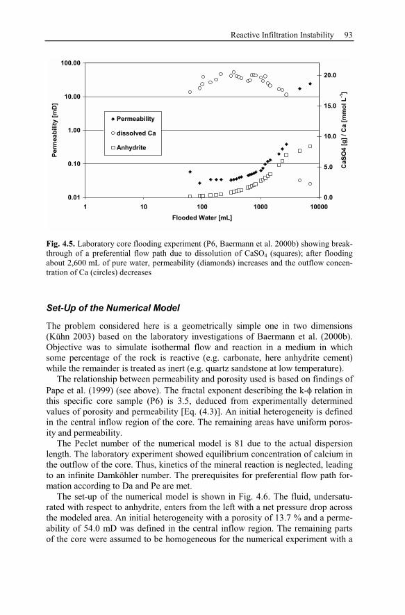
Reactive Infiltration Instability 93
0.01
0.10
1.00
10.00
100.00
1 10 100 1000 10000
Flooded Water [mL]
Perm
eab
ilit
y [
mD
]
0.0
5.0
10.0
15.0
20.0
CaS
O4 [
g]
/ C
a [
mm
ol L
-1]
Permeability
dissolved Ca
Anhydrite
Fig. 4.5. Laboratory core flooding experiment (P6, Baermann et al. 2000b) showing break-
through of a preferential flow path due to dissolution of CaSO4 (squares); after flooding
about 2,600 mL of pure water, permeability (diamonds) increases and the outflow concen-
tration of Ca (circles) decreases
Set-Up of the Numerical Model
The problem considered here is a geometrically simple one in two dimensions
(Kühn 2003) based on the laboratory investigations of Baermann et al. (2000b).
Objective was to simulate isothermal flow and reaction in a medium in which
some percentage of the rock is reactive (e.g. carbonate, here anhydrite cement)
while the remainder is treated as inert (e.g. quartz sandstone at low temperature).
The relationship between permeability and porosity used is based on findings of
Pape et al. (1999) (see above). The fractal exponent describing the k-φ relation in
this specific core sample (P6) is 3.5, deduced from experimentally determined
values of porosity and permeability [Eq. (4.3)]. An initial heterogeneity is defined
in the central inflow region of the core. The remaining areas have uniform poros-
ity and permeability.
The Peclet number of the numerical model is 81 due to the actual dispersion
length. The laboratory experiment showed equilibrium concentration of calcium in
the outflow of the core. Thus, kinetics of the mineral reaction is neglected, leading
to an infinite Damköhler number. The prerequisites for preferential flow path for-
mation according to Da and Pe are met.
The set-up of the numerical model is shown in Fig. 4.6. The fluid, undersatu-
rated with respect to anhydrite, enters from the left with a net pressure drop across
the modeled area. An initial heterogeneity with a porosity of 13.7 % and a perme-
ability of 54.0 mD was defined in the central inflow region. The remaining parts
of the core were assumed to be homogeneous for the numerical experiment with a
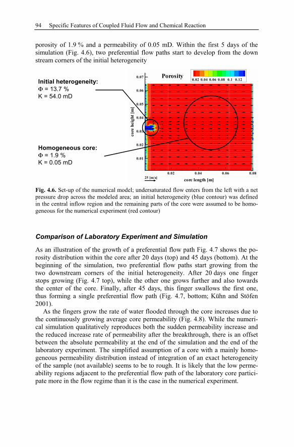
94 Specific Features of Coupled Fluid Flow and Chemical Reaction
porosity of 1.9 % and a permeability of 0.05 mD. Within the first 5 days of the
simulation (Fig. 4.6), two preferential flow paths start to develop from the down
stream corners of the initial heterogeneity
core length [m]
co
re
heig
ht
[m
]
0.02 0.04 0.06 0.08
0.01
0.02
0.03
0.04
0.05
0.06
0.070.02 0.04 0.06 0.08 0.1 0.12
Porosity
25 [m/a]
Initial heterogeneity:
Φ = 13.7 %
K = 54.0 mD
Homogeneous core:
Φ = 1.9 %
K = 0.05 mD
Fig. 4.6. Set-up of the numerical model; undersaturated flow enters from the left with a net
pressure drop across the modeled area; an initial heterogeneity (blue contour) was defined
in the central inflow region and the remaining parts of the core were assumed to be homo-
geneous for the numerical experiment (red contour)
Comparison of Laboratory Experiment and Simulation
As an illustration of the growth of a preferential flow path Fig. 4.7 shows the po-
rosity distribution within the core after 20 days (top) and 45 days (bottom). At the
beginning of the simulation, two preferential flow paths start growing from the
two downstream corners of the initial heterogeneity. After 20 days one finger
stops growing (Fig. 4.7 top), while the other one grows further and also towards
the center of the core. Finally, after 45 days, this finger swallows the first one,
thus forming a single preferential flow path (Fig. 4.7, bottom; Kühn and Stöfen
2001).
As the fingers grow the rate of water flooded through the core increases due to
the continuously growing average core permeability (Fig. 4.8). While the numeri-
cal simulation qualitatively reproduces both the sudden permeability increase and
the reduced increase rate of permeability after the breakthrough, there is an offset
between the absolute permeability at the end of the simulation and the end of the
laboratory experiment. The simplified assumption of a core with a mainly homo-
geneous permeability distribution instead of integration of an exact heterogeneity
of the sample (not available) seems to be to rough. It is likely that the low perme-
ability regions adjacent to the preferential flow path of the laboratory core partici-
pate more in the flow regime than it is the case in the numerical experiment.
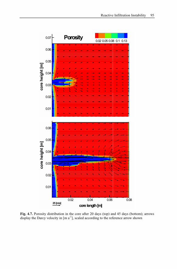
Reactive Infiltration Instability 95
co
reh
eig
ht
[m]
0.01
0.02
0.03
0.04
0.05
0.06
0.07
0.02 0.05 0.08 0.1 0.13Porosity
core length[m]
co
reh
eig
ht
[m]
0.02 0.04 0.06 0.08
0.01
0.02
0.03
0.04
0.05
0.06
25 [m/a]
Fig. 4.7. Porosity distribution in the core after 20 days (top) and 45 days (bottom); arrows
display the Darcy velocity in [m a-1
], scaled according to the reference arrow shown
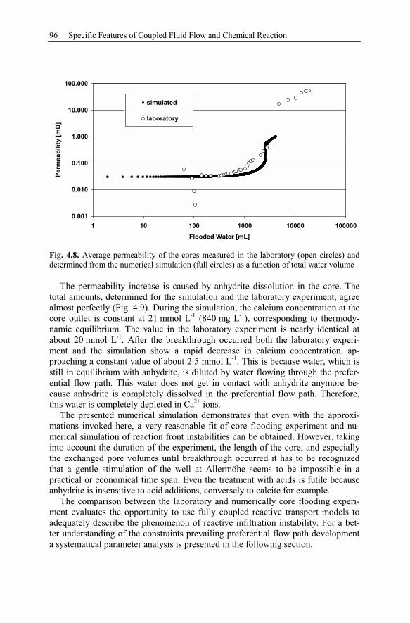
96 Specific Features of Coupled Fluid Flow and Chemical Reaction
0.001
0.010
0.100
1.000
10.000
100.000
1 10 100 1000 10000 100000
Flooded Water [mL]
Pe
rm
eab
ilit
y [
mD
]
simulated
laboratory
Fig. 4.8. Average permeability of the cores measured in the laboratory (open circles) and
determined from the numerical simulation (full circles) as a function of total water volume
The permeability increase is caused by anhydrite dissolution in the core. The
total amounts, determined for the simulation and the laboratory experiment, agree
almost perfectly (Fig. 4.9). During the simulation, the calcium concentration at the
core outlet is constant at 21 mmol L-1
(840 mg L-1
), corresponding to thermody-
namic equilibrium. The value in the laboratory experiment is nearly identical at
about 20 mmol L-1
. After the breakthrough occurred both the laboratory experi-
ment and the simulation show a rapid decrease in calcium concentration, ap-
proaching a constant value of about 2.5 mmol L-1
. This is because water, which is
still in equilibrium with anhydrite, is diluted by water flowing through the prefer-
ential flow path. This water does not get in contact with anhydrite anymore be-
cause anhydrite is completely dissolved in the preferential flow path. Therefore,
this water is completely depleted in Ca2+
ions.
The presented numerical simulation demonstrates that even with the approxi-
mations invoked here, a very reasonable fit of core flooding experiment and nu-
merical simulation of reaction front instabilities can be obtained. However, taking
into account the duration of the experiment, the length of the core, and especially
the exchanged pore volumes until breakthrough occurred it has to be recognized
that a gentle stimulation of the well at Allermöhe seems to be impossible in a
practical or economical time span. Even the treatment with acids is futile because
anhydrite is insensitive to acid additions, conversely to calcite for example.
The comparison between the laboratory and numerically core flooding experi-
ment evaluates the opportunity to use fully coupled reactive transport models to
adequately describe the phenomenon of reactive infiltration instability. For a bet-
ter understanding of the constraints prevailing preferential flow path development
a systematical parameter analysis is presented in the following section.
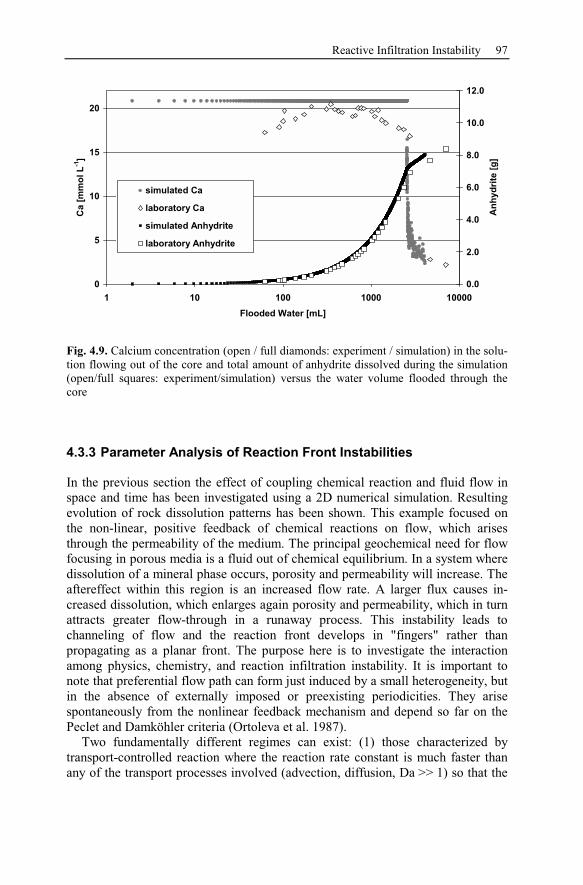
Reactive Infiltration Instability 97
0
5
10
15
20
1 10 100 1000 10000
Flooded Water [mL]
Ca
[m
mo
l L
-1]
0.0
2.0
4.0
6.0
8.0
10.0
12.0
An
hyd
rit
e [
g]
simulated Ca
laboratory Ca
simulated Anhydrite
laboratory Anhydrite
Fig. 4.9. Calcium concentration (open / full diamonds: experiment / simulation) in the solu-
tion flowing out of the core and total amount of anhydrite dissolved during the simulation
(open/full squares: experiment/simulation) versus the water volume flooded through the
core
4.3.3 Parameter Analysis of Reaction Front Instabilities
In the previous section the effect of coupling chemical reaction and fluid flow in
space and time has been investigated using a 2D numerical simulation. Resulting
evolution of rock dissolution patterns has been shown. This example focused on
the non-linear, positive feedback of chemical reactions on flow, which arises
through the permeability of the medium. The principal geochemical need for flow
focusing in porous media is a fluid out of chemical equilibrium. In a system where
dissolution of a mineral phase occurs, porosity and permeability will increase. The
aftereffect within this region is an increased flow rate. A larger flux causes in-
creased dissolution, which enlarges again porosity and permeability, which in turn
attracts greater flow-through in a runaway process. This instability leads to
channeling of flow and the reaction front develops in "fingers" rather than
propagating as a planar front. The purpose here is to investigate the interaction
among physics, chemistry, and reaction infiltration instability. It is important to
note that preferential flow path can form just induced by a small heterogeneity, but
in the absence of externally imposed or preexisting periodicities. They arise
spontaneously from the nonlinear feedback mechanism and depend so far on the
Peclet and Damköhler criteria (Ortoleva et al. 1987).
Two fundamentally different regimes can exist: (1) those characterized by
transport-controlled reaction where the reaction rate constant is much faster than
any of the transport processes involved (advection, diffusion, Da >> 1) so that the
98 Specific Features of Coupled Fluid Flow and Chemical Reaction
length scale over which a moving fluid comes to equilibrium is small. The exis-
tence and amplitude of channels in this reaction regime depend primarily on the
ratio of flow velocity to the dispersion coefficient (Pe number controlled). And (2)
those characterized by kinetic rate-controlled reaction where equilibrium between
the fluid and the reacting mineral occurs over some distance (Da < 1, Hoefner and
Fogler 1988). In this case permeability change is more diffuse. With decreasing
Da the efficiency of individual channel propagation decreases.
Steefel and Lasaga (1990) investigated in their numerical simulations the
propagation of a single finger dependent on the fixed ratio of advection and dis-
persion (Pe = 100) and dependent on the ratio between the reaction rate and advec-
tion both at a given and fixed length scale (10 m). They found that in cases of Da
numbers less than 0.01 any perturbation of a planar reaction front decays away.
The permeability change occurs over such a large distance that a channel cannot
propagate efficiently. However, in the transport-controlled regime, when the Da
number is large enough, the critical parameter is the Pe number, which ultimately
determines whether a channel propagates at all. Steefel and Lasaga (1990) con-
cluded that in cases of small advection to dispersion ratios channeling may de-
velop only on scales recognizable by regional mapping [compare Eq. (4.9)].
Ormond and Ortoleva (2000) performed simulations at the experimental scale
with large Pe and Da numbers, above 100 and 1, respectively. They actually var-
ied the width of the domain as well as the measure and number of the initial het-
erogeneity. They found that size and growth rate of fingers are independent of the
width of the initial heterogeneity. If the initial heterogeneity is wider than around
6.0x10⁻³
m two fingers develop from its downstream corners. But, those two fin-
gers do not grow too close to each other. In that case one finger stops growing and
the remaining finger becomes wider (compare example of Allermöhe core flood-
ing). Their second result is that the final finger width is independent on the meas-
ure or number of initial heterogeneities but ≈ 4 times the thickness of the reaction
front (≡ saturation length). Investigations of a homogeneous matrix perturbed by
an initial white noise at the domain’s inlet revealed that several fingers start to
grow. The elongation of every finger depends in the following on the competition
between them to capture the fluid flow. Finally, width and number of developing
preferential flow paths are determined by the flow and reaction characteristics of
the system (Pe and Da). The progress of any finger itself is directly related to the
magnitude of flow. However, the length of an elongated channel depends on the
balance between advection and dispersion: If dispersion equilibrates concentration
inside the channel before the fluid reaches the channel tip, growth stops.
Based on the systematic studies of Steefel and Lasage (1990) and Ormond and
Ortoleva (2000) the interaction of the Pe and Da numbers on the development of
preferential flow path is investigated here.
Model Components for the Parameter Analysis
Concerning rock properties, the problem formulated here for the parameter analy-
sis is essentially the same as the one considered above (Allermöhe core P6). Thus,
Reactive Infiltration Instability 99
preferential flow path development within the Allermöhe cores and in general is
understood in more detail.
The simulations conducted comprise a range of dimensionless numbers. The
Peclet number varies between 1 and 500 and the Damköhler number from 0.003 to
infinite (thermodynamic equilibrium). The systems investigated measured 2.0 re-
spectively 3.0 cm in height. The model length is 8.0 cm for all studies and they are
discretized in cells measuring 1 by 1 mm. The systems investigated are listed in
Table 4.1.
Table 4.1. Systems used for the parameter analysis, characterized by the total number of
cells, Pe and Da numbers, and the applied heterogeneity; cell dimensions are 1 x 1 mm in
all cases
Number of cells Pe number Da number Heterogeneity
20 x 80 1, 2, 5, 10, 20, 30, 40,
50, 60, 70, 80, 90,
100, 200
0.003, 0.03, 0.06,
0.09, 0.12, 0.15,
0.3, 0.6, 0.9, 1.2,
3.0, ∞
0.002 m x 0.004 m
30 x 80 3, 5, 10, 30, 50, 100,
300, 500
0.15, 0.3, 1.5, 3.0,
∞white noise
The investigated systems are used to conduct simulations for different pur-
poses. Systematic studies are done to get insight in the following topics:
• Development of one channel induced by a single heterogeneity measuring 2 x
4 mm at the center of the inflow within a homogeneous core (20 x 80).
• Onset of reaction front instabilities, development either of a planar front or
preferential flow paths, dependent on the Peclet and Damköhler numbers in-
duced by a heterogeneous distribution of the core inlet or within the entire re-
gion of the core (30 x 80).
Development of One Channel
The first study done with varying Damköhler (Da) and Peclet (Pe) numbers is to
show the development of a single channel from a single rectangular heterogeneity.
The heterogeneity is placed at the core inlet (no anhydrite, 2 x 4 mm) within a
homogeneous system of 20 x 80 cells measuring 1 x 1 mm each. Da numbers in-
vestigated and displayed in Fig. 4.10 and Fig. 4.11 are 0.03, 0.3, 3.0, and infinite
in combination with Pe numbers 1, 5, 10, 20, 30, 50, 70, and 100.
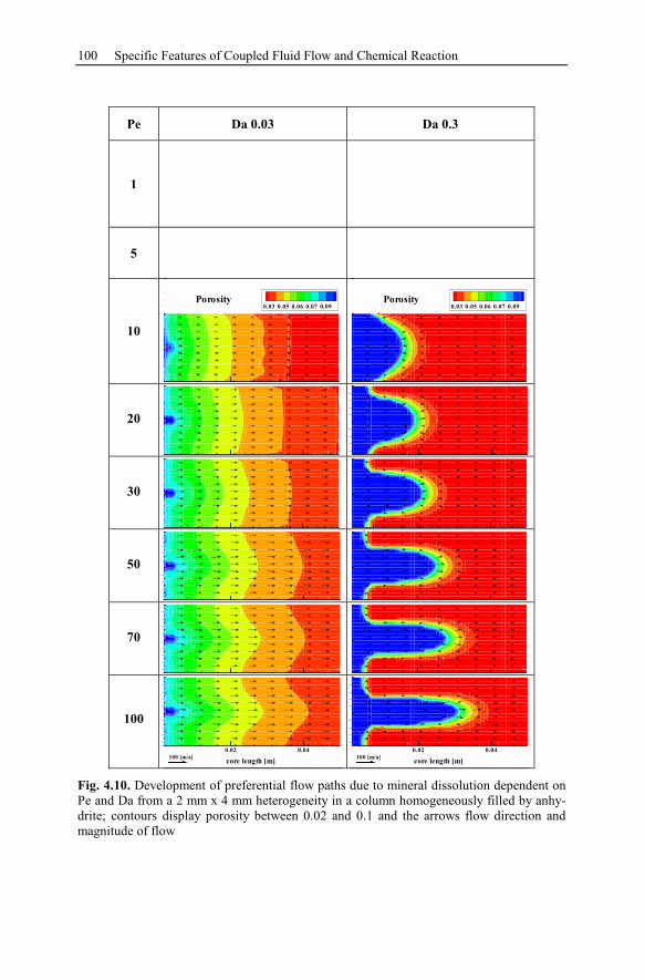
100 Specific Features of Coupled Fluid Flow and Chemical Reaction
Pe Da 0.03 Da 0.3
1
5
10
0.03 0.05 0.06 0.07 0.09
Porosity0.03 0.05 0.06 0.07 0.09
Porosity
20
30
50
70
100
core length [m]
0.02 0.04
100 [m/a]core length [m]
0.02 0.04
100 [m/a]
Fig. 4.10. Development of preferential flow paths due to mineral dissolution dependent on
Pe and Da from a 2 mm x 4 mm heterogeneity in a column homogeneously filled by anhy-
drite; contours display porosity between 0.02 and 0.1 and the arrows flow direction and
magnitude of flow
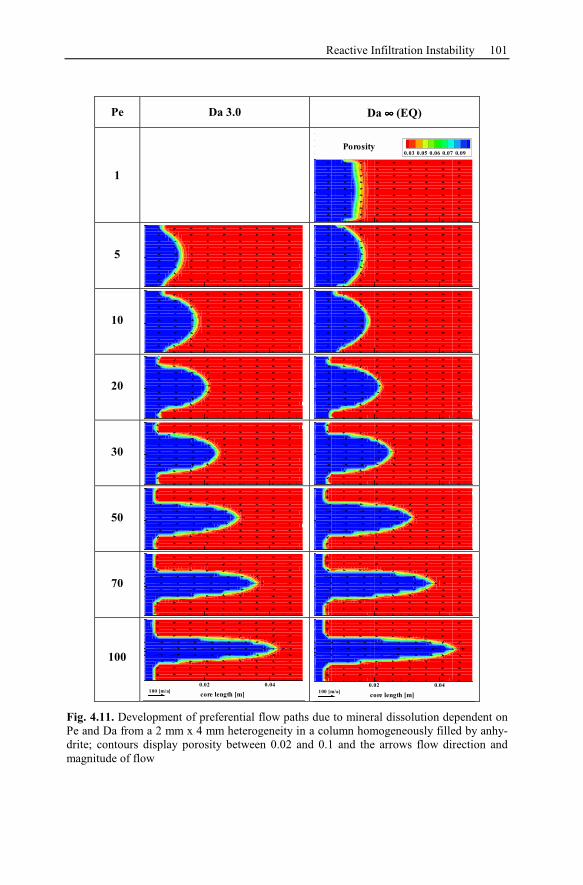
Reactive Infiltration Instability 101
Pe Da 3.0 Da ∞∞∞∞ (EQ)
1
0.03 0.05 0.06 0.07 0.09
Porosity
5
10
20
30
50
70
100
core length [m]
0.02 0.04
100 [m/a]
core length [m]
0.02 0.04
100 [m/a]
Fig. 4.11. Development of preferential flow paths due to mineral dissolution dependent on
Pe and Da from a 2 mm x 4 mm heterogeneity in a column homogeneously filled by anhy-
drite; contours display porosity between 0.02 and 0.1 and the arrows flow direction and
magnitude of flow
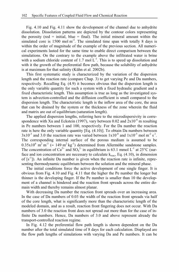
102 Specific Features of Coupled Fluid Flow and Chemical Reaction
Fig. 4.10 and Fig. 4.11 show the development of the channel due to anhydrite
dissolution. Dissolution patterns are depicted by the contour colors representing
the porosity (red = initial, blue = final). The initial mineral amount within the
simulated core is 1500 mol m-3
. The simulated time span with totally 8 days is
within the order of magnitude of the example of the previous section. All numeri-
cal experiments lasted for the same time to enable direct comparison between the
simulations. On the contrary to the example above the infiltrated water is brine
with a sodium chloride content of 1.7 mol L-1
. This is to speed up dissolution and
with it the growth of the preferential flow path, because the solubility of anhydrite
is at maximum for that salinity (Kühn et al. 2002b).
This first systematic study is characterized by the variation of the dispersion
length and the reaction rate (compare Chap. 3) to get varying Pe and Da numbers,
respectively. Recalling Eq. (4.9) it becomes obvious that the dispersion length is
the only variable quantity for such a system with a fixed hydraulic gradient and a
fixed characteristic length. This assumption is true as long as the investigated sys-
tem is advection-controlled and the diffusion coefficient is small compared to the
dispersion length. The characteristic length is the inflow area of the core, the area
that can be drained by the system or the thickness of the zone wherein the fluid
and matrix are out of equilibrium (saturation length).
The applied dispersion lengths, referring here to the microdispersivity in corre-
spondence with Xu and Eckstein (1997), vary between 0.02 and 2x10⁻⁴
m resulting
in Pe numbers between 1 and 100, respectively. For the Da number the reaction
rate is here the only variable quantity [Eq. (4.10)]. To obtain Da numbers between
3x10⁻³
and 3.0 the reaction rate was varied between 1x10⁻⁸
and 1x10⁻⁵
mol m-2
s-1
.
The corresponding internal surface of the porous medium is assumed to be
0.35x10⁶ m
2 m
-3 (≈ 149 m
2 kg
-1) determined from Allermöhe sandstone samples.
The concentration of Ca2+
and SO4
2- in equilibrium is 63.1 mmol L
-1 at 25°C (sur-
face and ion concentration are necessary to calculate kreac, Eq. (4.10), in dimension
of [s-1
]). An infinite Da number is given when the reaction rate is infinite, repre-
senting thermodynamic equilibrium between the solution and the mineral phase.
The initial conditions force the active development of one single finger. It is
obvious from Fig. 4.10 and Fig. 4.11 that the higher the Pe number the longer but
thinner is the developing finger. If the Pe number is smaller than 10 the develop-
ment of a channel is hindered and the reaction front spreads across the entire do-
main width and thereby remains almost planar.
With decreasing Da number the reaction front spreads over an increasing area.
In the case of Da numbers of 0.03 the width of the reaction front spreads via half
of the core length, what is significantly more than the characteristic length of the
modeled domain, and as a result, reaction front fingering does not occur. With Da
numbers of 3.0 the reaction front does not spread out more than for the case of in-
finite Da numbers. Hence, Da numbers of 3.0 and above represent already the
transport-controlled reaction regime.
In Fig. 4.12 the preferential flow path length is shown dependent on the Da
number after the total simulated time of 8 days for each calculation. Displayed are
the flow path lengths of simulations with varying Da and Pe numbers. It can be
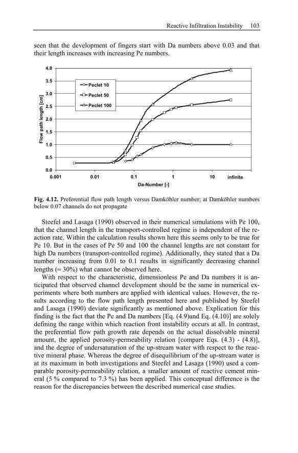
Reactive Infiltration Instability 103
seen that the development of fingers start with Da numbers above 0.03 and that
their length increases with increasing Pe numbers.
0.0
0.5
1.0
1.5
2.0
2.5
3.0
3.5
4.0
0.001 0.01 0.1 1 10 100
Da-Number [-]
Flo
w p
ath
len
gth
[cm
]
Peclet 10
Peclet 50
Peclet 100
infinite
Fig. 4.12. Preferential flow path length versus Damköhler number; at Damköhler numbers
below 0.07 channels do not propagate
Steefel and Lasaga (1990) observed in their numerical simulations with Pe 100,
that the channel length in the transport-controlled regime is independent of the re-
action rate. Within the calculation results shown here this seems only to be true for
Pe 10. But in the cases of Pe 50 and 100 the channel lengths are not constant for
high Da numbers (transport-controlled regime). Additionally, they stated that a Da
number increasing from 0.01 to 0.1 results in significantly decreasing channel
lengths (≈ 30%) what cannot be observed here.
With respect to the characteristic, dimensionless Pe and Da numbers it is an-
ticipated that observed channel development should be the same in numerical ex-
periments where both numbers are applied with identical values. However, the re-
sults according to the flow path length presented here and published by Steefel
and Lasaga (1990) deviate significantly as mentioned above. Explication for this
finding is the fact that the Pe and Da numbers [Eq. (4.9)and Eq. (4.10)] are solely
defining the range within which reaction front instability occurs at all. In contrast,
the preferential flow path growth rate depends on the actual dissolvable mineral
amount, the applied porosity-permeability relation [compare Eqs. (4.3) - (4.8)],
and the degree of undersaturation of the up-stream water with respect to the reac-
tive mineral phase. Whereas the degree of disequilibrium of the up-stream water is
at its maximum in both investigations and Steefel and Lasaga (1990) used a com-
parable porosity-permeability relation, a smaller amount of reactive cement min-
eral (5 % compared to 7.3 %) has been applied. This conceptual difference is the
reason for the discrepancies between the described numerical case studies.
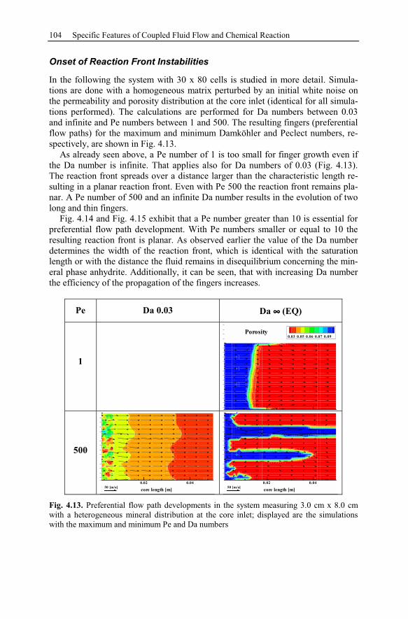
104 Specific Features of Coupled Fluid Flow and Chemical Reaction
Onset of Reaction Front Instabilities
In the following the system with 30 x 80 cells is studied in more detail. Simula-
tions are done with a homogeneous matrix perturbed by an initial white noise on
the permeability and porosity distribution at the core inlet (identical for all simula-
tions performed). The calculations are performed for Da numbers between 0.03
and infinite and Pe numbers between 1 and 500. The resulting fingers (preferential
flow paths) for the maximum and minimum Damköhler and Peclect numbers, re-
spectively, are shown in Fig. 4.13.
As already seen above, a Pe number of 1 is too small for finger growth even if
the Da number is infinite. That applies also for Da numbers of 0.03 (Fig. 4.13).
The reaction front spreads over a distance larger than the characteristic length re-
sulting in a planar reaction front. Even with Pe 500 the reaction front remains pla-
nar. A Pe number of 500 and an infinite Da number results in the evolution of two
long and thin fingers.
Fig. 4.14 and Fig. 4.15 exhibit that a Pe number greater than 10 is essential for
preferential flow path development. With Pe numbers smaller or equal to 10 the
resulting reaction front is planar. As observed earlier the value of the Da number
determines the width of the reaction front, which is identical with the saturation
length or with the distance the fluid remains in disequilibrium concerning the min-
eral phase anhydrite. Additionally, it can be seen, that with increasing Da number
the efficiency of the propagation of the fingers increases.
Pe Da 0.03 Da ∞∞∞∞ (EQ)
1
0.03 0.05 0.06 0.07 0.09
Porosity
500
core length [m]
0.02 0.04
50 [m/a]core length [m]
0.02 0.04
50 [m/a]
Fig. 4.13. Preferential flow path developments in the system measuring 3.0 cm x 8.0 cm
with a heterogeneous mineral distribution at the core inlet; displayed are the simulations
with the maximum and minimum Pe and Da numbers
Reactive Infiltration Instability 105
Generally, it can be observed that the finger length increases with increasing Pe
number. Simultaneously, the finger width is decreasing. The higher the Pe number
the thinner are the developing preferential flow paths.
The first and necessary requirement for preferential flow path development is a
Peclet number above ten. If this is the case a reactive flow system is eligible for
self-organized reaction front instabilities resulting in channel development. The
second but self-sufficient requirement, the Damköhler number, defines the scale
on which fingering reactions are possible. The characteristic length of a system,
identical with the maximum drainable area, must be larger than the width of the
reaction front or the saturation length of the particular reaction. In other words, if
the reaction rate is small, the characteristic length must be sufficiently large (e.g.
in this case the system must be of adequate height) to get a Da number in the sys-
tem under consideration that is at least above 0.03 (Fig. 4.12).
Within the numerical experiments with Pe numbers smaller or equal to ten and
Da numbers of 1.5 and 3.0 (Fig. 4.15) it can be observed that fingering seems to
occur at the upper and lower boundary of the model, although preferential flow
paths should not develop (Pe ≤ 10, see above). To further investigate this phe-
nomenon, additional numerical experiments were conducted. The upper and lower
model boundaries were assumed as impervious so far, according to a laboratory
core flooding experiment. Fig. 4.18 displays the results of two numerical simula-
tions where the overall time has been split into four periods of two days each.
Conversely to the previous calculations one simulation was performed with "en-
abled" dispersive and diffusive transport via the model boundaries. Such an ex-
periment corresponds to a natural system with a permeable layer surrounded by
material of low permeability but not impervious. Both simulations were conducted
with a Pe number of ten and an infinite Da number. In comparison to the previ-
ously performed simulations with totally impervious boundaries there is no finger-
ing at the model edges observable in this case (Fig. 4.18). Hence, it can be inferred
that impervious boundaries, leading to decreased dispersivities and resulting in in-
creased Pe numbers [Eq. (4.9)], might cause fingering processes directly at the
border of the modeled system. This indicates especially for laboratory core flood-
ing experiments that channel development at the margins has to be taken into ac-
count.
Finally, simulations of preferential flow path development were done in a fully
heterogeneous system according to the mineral, porosity, and permeability distri-
bution (Fig. 4.16 and Fig. 4.17). The same number of preferential flow paths de-
velops at identical locality. The only difference to the previous observations and
conclusions is the fact that the increased heterogeneity of the cores leads to a de-
creased efficiency of the channel propagation. The fingering process is slower,
another argument against the feasibility of gentle stimulation of the Allermöhe
well (see core flooding experiment above)
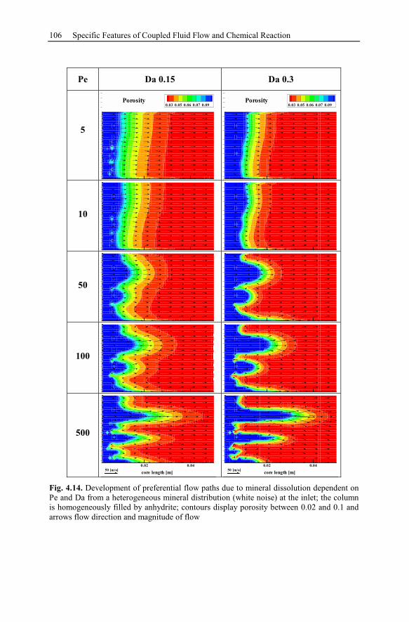
106 Specific Features of Coupled Fluid Flow and Chemical Reaction
Pe Da 0.15 Da 0.3
5
0.03 0.05 0.06 0.07 0.09
Porosity0.03 0.05 0.06 0.07 0.09
Porosity
10
50
100
500
core length [m]
0.02 0.04
50 [m/a]core length [m]
0.02 0.04
50 [m/a]
Fig. 4.14. Development of preferential flow paths due to mineral dissolution dependent on
Pe and Da from a heterogeneous mineral distribution (white noise) at the inlet; the column
is homogeneously filled by anhydrite; contours display porosity between 0.02 and 0.1 and
arrows flow direction and magnitude of flow
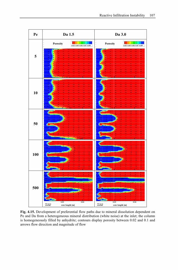
Reactive Infiltration Instability 107
Pe Da 1.5 Da 3.0
5
0.03 0.05 0.06 0.07 0.09
Porosity0.03 0.05 0.06 0.07 0.09
Porosity
10
50
100
500
core length [m]
0.02 0.04
50 [m/a]core length [m]
0.02 0.04
50 [m/a]
Fig. 4.15. Development of preferential flow paths due to mineral dissolution dependent on
Pe and Da from a heterogeneous mineral distribution (white noise) at the inlet; the column
is homogeneously filled by anhydrite; contours display porosity between 0.02 and 0.1 and
arrows flow direction and magnitude of flow
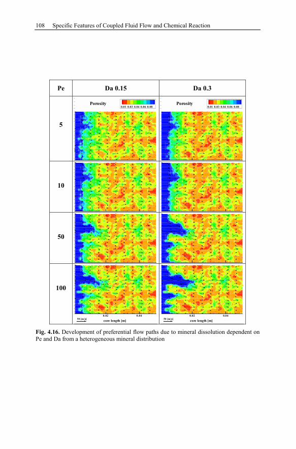
108 Specific Features of Coupled Fluid Flow and Chemical Reaction
Pe Da 0.15 Da 0.3
5
0.01 0.03 0.04 0.06 0.08
Porosity0.01 0.03 0.04 0.06 0.08
Porosity
10
50
100
core length [m]
0.02 0.04
50 [m/a]core length [m]
0.02 0.04
50 [m/a]
Fig. 4.16. Development of preferential flow paths due to mineral dissolution dependent on
Pe and Da from a heterogeneous mineral distribution
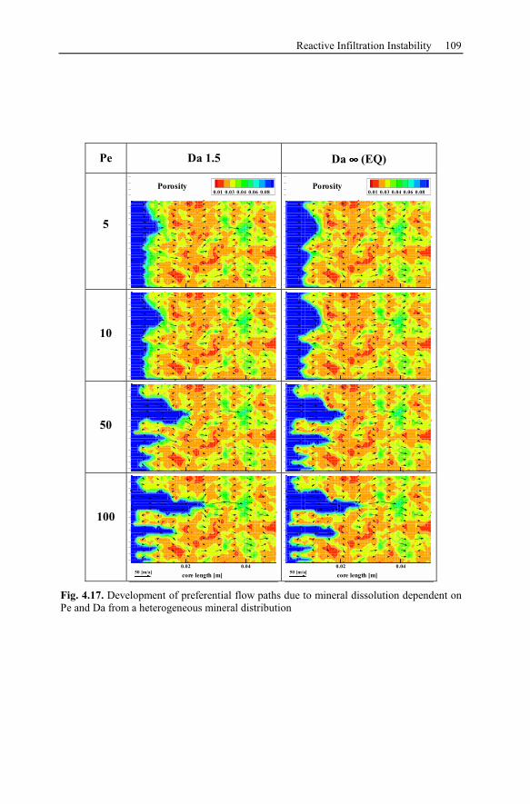
Reactive Infiltration Instability 109
Pe Da 1.5 Da ∞∞∞∞ (EQ)
5
0.01 0.03 0.04 0.06 0.08
Porosity0.01 0.03 0.04 0.06 0.08
Porosity
10
50
100
core length [m]
0.02 0.04
50 [m/a]core length [m]
0.02 0.04
50 [m/a]
Fig. 4.17. Development of preferential flow paths due to mineral dissolution dependent on
Pe and Da from a heterogeneous mineral distribution
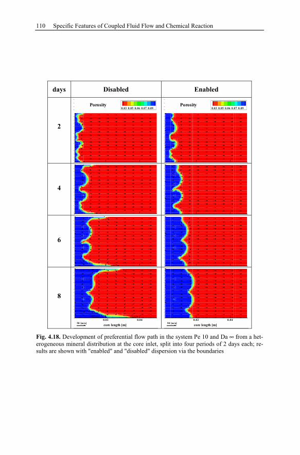
110 Specific Features of Coupled Fluid Flow and Chemical Reaction
days Disabled Enabled
2
0.03 0.05 0.06 0.07 0.09
Porosity0.03 0.05 0.06 0.07 0.09
Porosity
4
6
8
core length [m]
0.02 0.04
50 [m/a]core length [m]
0.02 0.04
50 [m/a]
Fig. 4.18. Development of preferential flow path in the system Pe 10 and Da ∞ from a het-
erogeneous mineral distribution at the core inlet, split into four periods of 2 days each; re-
sults are shown with "enabled" and "disabled" dispersion via the boundaries
Thermal Convection 111
4.4 Thermal Convection
Several driving mechanisms for large-scale fluid flow in sedimentary basins have
been proposed, including: (1) topography- or gravity driven flow (Garven and
Freeze 1984); (2) compaction-driven flow during basin subsidence (Cathles and
Smith 1983, Bethke 1985); (3) seismic pumping and tectonically driven flow (Sib-
son et al. 1975, Oliver 1986); and (4) buoyancy-driven flow, including thermal
driven or free convection (Cathles 1981, Bjorlykke et al. 1988).
Muffler (1985) considered free thermal convection to be a potential mechanism
for mass and heat transport in sedimentary basins. Diagenetic processes in sedi-
mentary basins involve reactions between pore water and mineral phases during
which unstable minerals are dissolved and more stable phases are precipitated.
These reactions are controlled by thermodynamic stability and reaction kinetics.
Spatial variations in temperature and pressure are assumed to be responsible for
much of the cementation and dissolution observed in rocks at depth. Muffler
(1985) presumed that fluid transport by thermal convection might operate under
such gradients to enhance diagenetic cementation processes. Theoretical investiga-
tions of heat transport in sandstone layers indicate that common geometries related
to geologic structure can give rise to internal convection cells. Most geothermal
development to date for example has been carried out in hydrothermal convection
systems. Near-surface temperatures are increased in hydrothermal systems by the
movement of hot water through pores and fractures (Muffler 1985).
Wood and Hewett (1982) showed that eddy currents of large scale (km) spon-
taneously arise and persist in porous, fluid-saturated geologic formations, when
these systems are subjected to normal geothermal temperature gradients (25-
30°C km-1
). They assume that the velocity of these fluid currents is on the order of
1 m per year. Such a mass flux may produce significant porosity changes when it
prolongs over a period of several million years. Hence, post-depositional reservoir
cementation might be due to slowly circulating fluids.
Bjorlykke et al. (1988) studied the onset of free convection in a layered system
and concluded that even small (< 1 m) low-permeability layers could effectively
split a system and inhibit free convection systems. On the contrary to the proposi-
tions of Muffler (1985) and Wood and Hewett (1982) it is currently accepted that
free convection is unlikely to occur in most sedimentary basins except under cer-
tain unique conditions, such as very high basal heat fluxes or unusually thick and
permeable formations (Bjorlykke et al. 1988, Raffensberger and Garven 1995), or
in the vicinity of igneous intrusions (Norton and Knight 1977) or salt domes
(Hanor 1987, Evans and Nunn 1989). However, in the following section (compare
Chap. 5) it will be shown that free convection has to be distinguished into "verti-
cal" and "horizontal" currents. Although "vertical" free convection is most
unlikely to occur, free "horizontal" convection has to be taken into account under
particular geologic circumstances. Nevertheless, the principles of "vertical" con-
112 Specific Features of Coupled Fluid Flow and Chemical Reaction
vection systems will be described here to clarify how diagenetic reactions (e.g.
cementation) can be explained by reactive transport due to buoyancy-driven flow.
4.4.1 Rayleigh Number
The dimensionless Rayleigh number Ra [Eq. (4.11)] indicates the tendency to-
wards free convection, that is, flow driven purely by density differences. Classic
Rayleigh convection theory was developed in the context of an infinite, perme-
able, horizontal layer bounded at top and bottom by isothermal, impermeable for-
mations. The Rayleigh number is based on the ratio of "buoyant" forces that drive
convective fluid flow to the viscous forces inhibiting fluid movement. The value
of Ra is given by:
( )2
W W W L U
W m
c g k L T TRa
α ⋅ ρ ⋅ ⋅ ⋅ ⋅ ⋅ −=
µ ⋅ λ(4.11)
where W is thermal expansivity of water (°C-1
), ρW density of water (kg m-3
), cW
isochoric heat capacity (J kg-1
K-1
), g gravitational acceleration (m s-2
), k intrinsic
permeability (m2), L characteristic length (m, formation thickness), T temperature
(K, L: lower boundary, U: upper boundary), µW dynamic viscosity (kg m-1
s-1
),
and λm thermal conductivity of the medium (J s-1
m-1
K-1
, rock formation). Lap-
wood (1948) showed that the fluid in an infinite horizontal layer would begin to
convect at a critical Ra value of 42. There is no critical Ra number for any non-
isothermal sloping layer, and all such layers should have fluids circulating at some
finite velocity (Ingebritsen and Sanford 1998).
Sorey (1978) noted that if (TL-TU) is large enough, the values of relevant fluid
properties ( W, W, cW, µW) as evaluated at TL and TU will be significantly differ-
ent and the corresponding Ra values at TL and TU will be as large as 60 and low as
2, respectively. In these cases a mean Ra number has to be taken into account.
Raffensberger and Vlassopoulos (1999) performed a series of numerical simu-
lations to investigate the influence of varying thicknesses and temperature gradi-
ents on the Ra number and resulting flow rates due to occurring free convection.
They determined that the correlation between the flow rate qfree (m yr-1
) and the
mean Ra number is best described by a second-order polynomial relationship:
2
c c
free 0.375 0.375
Ra Ra Ra Ra
q 1.2 0.17
L L
− −= + (4.12)
where Rac is the critical mean Rayleigh number for the onset of free convection
(42=39.478). This relationship allows for predicting the maximum flow rate
within an aquifer as a function of layer thickness, intrinsic permeability, viscosity,
and thermal properties of the fluid and the rock formation.
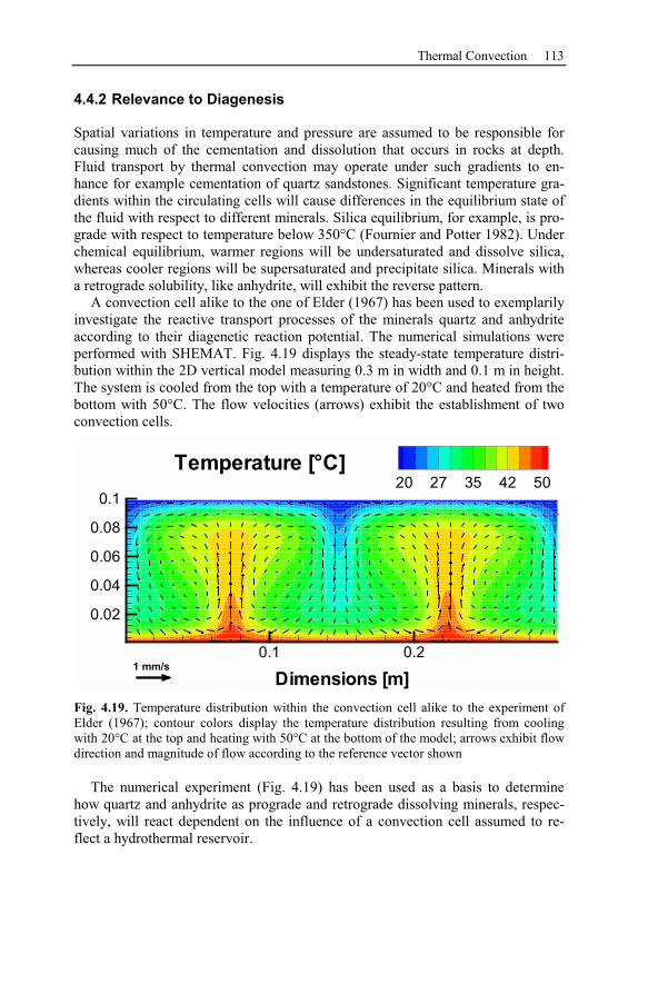
Thermal Convection 113
4.4.2 Relevance to Diagenesis
Spatial variations in temperature and pressure are assumed to be responsible for
causing much of the cementation and dissolution that occurs in rocks at depth.
Fluid transport by thermal convection may operate under such gradients to en-
hance for example cementation of quartz sandstones. Significant temperature gra-
dients within the circulating cells will cause differences in the equilibrium state of
the fluid with respect to different minerals. Silica equilibrium, for example, is pro-
grade with respect to temperature below 350°C (Fournier and Potter 1982). Under
chemical equilibrium, warmer regions will be undersaturated and dissolve silica,
whereas cooler regions will be supersaturated and precipitate silica. Minerals with
a retrograde solubility, like anhydrite, will exhibit the reverse pattern.
A convection cell alike to the one of Elder (1967) has been used to exemplarily
investigate the reactive transport processes of the minerals quartz and anhydrite
according to their diagenetic reaction potential. The numerical simulations were
performed with SHEMAT. Fig. 4.19 displays the steady-state temperature distri-
bution within the 2D vertical model measuring 0.3 m in width and 0.1 m in height.
The system is cooled from the top with a temperature of 20°C and heated from the
bottom with 50°C. The flow velocities (arrows) exhibit the establishment of two
convection cells.
Dimensions [m]
0.1 0.2
0.02
0.04
0.06
0.08
0.1
20 27 35 42 50
Temperature [°C]
1 mm/s
Fig. 4.19. Temperature distribution within the convection cell alike to the experiment of
Elder (1967); contour colors display the temperature distribution resulting from cooling
with 20°C at the top and heating with 50°C at the bottom of the model; arrows exhibit flow
direction and magnitude of flow according to the reference vector shown
The numerical experiment (Fig. 4.19) has been used as a basis to determine
how quartz and anhydrite as prograde and retrograde dissolving minerals, respec-
tively, will react dependent on the influence of a convection cell assumed to re-
flect a hydrothermal reservoir.
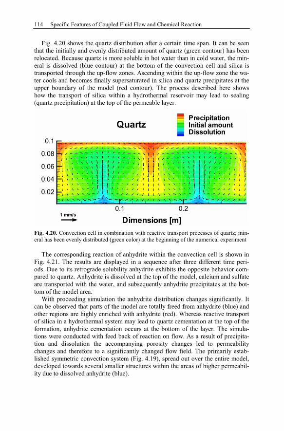
114 Specific Features of Coupled Fluid Flow and Chemical Reaction
Fig. 4.20 shows the quartz distribution after a certain time span. It can be seen
that the initially and evenly distributed amount of quartz (green contour) has been
relocated. Because quartz is more soluble in hot water than in cold water, the min-
eral is dissolved (blue contour) at the bottom of the convection cell and silica is
transported through the up-flow zones. Ascending within the up-flow zone the wa-
ter cools and becomes finally supersaturated in silica and quartz precipitates at the
upper boundary of the model (red contour). The process described here shows
how the transport of silica within a hydrothermal reservoir may lead to sealing
(quartz precipitation) at the top of the permeable layer.
Dimensions [m]
0.1 0.2
0.02
0.04
0.06
0.08
0.1
10010
9995
9979
Quartz
1 mm/s
Precipitation
Initial amount
Dissolution
Fig. 4.20. Convection cell in combination with reactive transport processes of quartz; min-
eral has been evenly distributed (green color) at the beginning of the numerical experiment
The corresponding reaction of anhydrite within the convection cell is shown in
Fig. 4.21. The results are displayed in a sequence after three different time peri-
ods. Due to its retrograde solubility anhydrite exhibits the opposite behavior com-
pared to quartz. Anhydrite is dissolved at the top of the model, calcium and sulfate
are transported with the water, and subsequently anhydrite precipitates at the bot-
tom of the model area.
With proceeding simulation the anhydrite distribution changes significantly. It
can be observed that parts of the model are totally freed from anhydrite (blue) and
other regions are highly enriched with anhydrite (red). Whereas reactive transport
of silica in a hydrothermal system may lead to quartz cementation at the top of the
formation, anhydrite cementation occurs at the bottom of the layer. The simula-
tions were conducted with feed back of reaction on flow. As a result of precipita-
tion and dissolution the accompanying porosity changes led to permeability
changes and therefore to a significantly changed flow field. The primarily estab-
lished symmetric convection system (Fig. 4.19), spread out over the entire model,
developed towards several smaller structures within the areas of higher permeabil-
ity due to dissolved anhydrite (blue).
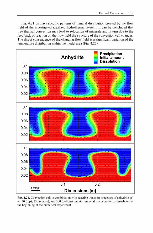
Thermal Convection 115
Fig. 4.21 displays specific patterns of mineral distribution created by the flow
field of the investigated idealized hydrothermal system. It can be concluded that
free thermal convection may lead to relocation of minerals and in turn due to the
feed back of reaction on the flow field the structure of the convection cell changes.
The direct consequence of the changing flow field is a significant variation of the
temperature distribution within the model area (Fig. 4.22).
0.02
0.04
0.06
0.08
0.1
1155
938
721
AnhydritePrecipitation
Initial amount
Dissolution
0.02
0.04
0.06
0.08
0.1
721
Dimensions [m]
0.1 0.2
0.02
0.04
0.06
0.08
0.1
721
1 mm/s
Fig. 4.21. Convection cell in combination with reactive transport processes of anhydrite af-
ter 30 (top), 150 (center), and 300 (bottom) minutes; mineral has been evenly distributed at
the beginning of the numerical experiment
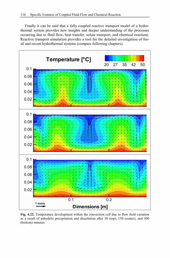
116 Specific Features of Coupled Fluid Flow and Chemical Reaction
Finally it can be said that a fully coupled reactive transport model of a hydro-
thermal system provides new insights and deeper understanding of the processes
occurring due to fluid flow, heat transfer, solute transport, and chemical reactions.
Reactive transport simulation provides a tool for the detailed investigation of fos-
sil and recent hydrothermal systems (compare following chapters).
0.02
0.04
0.06
0.08
0.1
20 27 35 42 50
Temperature [°C]
0.02
0.04
0.06
0.08
0.1
Dimensions [m]
0.1 0.2
0.02
0.04
0.06
0.08
0.1
1 mm/s
Fig. 4.22. Temperature development within the convection cell due to flow field variation
as a result of anhydrite precipitation and dissolution after 30 (top), 150 (center), and 300
(bottom) minutes
5 Fossil Hydrothermal Systems
Reactive transport modeling of the history of fossil hydrothermal systems provides
the basis for understanding genesis of ore deposits as well as progress of
diagenetic processes. The first part of this chapter presents a brief overview about
applications of numerical simulations done by other authors investigating these
topics. This is followed by a detailed examination of possible formation scenarios
for the observed and considerable anhydrite cementation found at the location Al-
lermöhe in Germany. For that purpose the SHEMAT software has been used in
order to numerically determine the thermal-reactive flow-deformational history of
the site. In order to explain the observed anhydrite cementation against the back-
ground of the entire geologic history of the Allermöhe site the fluid flow, heat
transfer, transport, and chemical reaction model has been coupled with a sequence
of geologic structures reflecting the stratigraphic development of the site.
5.1 Ore Deposits and Diagenesis
5.1.1 Ore Deposits
Most economically significant ore deposits exist because of the advective trans-
port of solutes and heat by flowing groundwater. Mobilization, transport, and
deposition of chemical species are all linked to fluid flow and most often to fossil
hydrothermal systems.
Reed (1983) applied a polythermal reaction model (see Chap. 3) to establish a
genetic link between massive sulfide deposits resting on metamorphic volcanic
rocks. Hereby, the reaction of heated seawater with the rocks of a volcanic pile is
assumed to be responsible for regional greenschist grade metamorphism. The so-
lution resulting from rock-water interaction is the source for copper, zinc, and iron
sulfide ore deposition in and on the basaltic rocks.
Lu et al. (1992) used a titration model (see Chap. 3) to interpret zinc-lead skarn
mineralization at Tin Creek, Alaska. The calculations were carried out using the
computer program CHILLER by stepwise titration of reactant rock into the fluid at
300°C. The concept of the model can be regarded as a single reaction front where
early-formed minerals can back-react because the fluid does not move away from
the reaction site. Lu et al. (1992) concluded that the thermal gradient, progressive
fluid reactions, and continuous interaction and dilution of hydrothermal fluids
might be responsible for the development of skarn zonation in the Tin Creek area.
Michael Kuhn: LNES 103, pp. 117–156, 2004.c© Springer-Verlag Berlin Heidelberg 2004
118 Fossil Hydrothermal Systems
Plumlee (1994) used the program CHILLER to study fluid chemistry evolution
and mineral deposition in the main-stage Creede epithermal system. The reaction
path calculations showed observed mineralogical variations are best accounted for
by boiling of the hydrothermal brines, followed by lateral mixing with overlying
dilute, steam-heated groundwaters. Conclusion is that epithermal mineral assem-
blages and zoning patterns can be used to reconstruct the paleohydrology of
hydrothermal systems.
The Ozark region of the North American mid-continent hosts a number of Mis-
sissippi Valley-Type (MVT) ore deposits. Most of these MVT deposits formed
from enormous hydrothermal systems in which fluid flow was driven topographi-
cally and tectonically. Beside a comprehensive discussion of host rocks, mineral-
ogy, and alteration processes of several districts from the Ozark region, Plumlee et
al. (1995b) performed reaction path modeling with CHILLER providing insights
into the ore formation processes applicable to MVT deposits worldwide. They
concluded that diverse hydrothermal mineral assemblages could be produced from
the same migrating basinal brine by different processes such as boiling, cooling,
water-rock interaction, and fluid mixing.
5.1.2 Diagenesis
With the burial of geological layers in sedimentary basins to depths of many kilo-
meters, several diagenetic reactions occur as a result of increasing pressure and
temperature. Firstly, this is the process of cementation (precipitation) by silica,
calcite, or iron and vice versa their dissolution. A second important group of proc-
esses is due to reactions with clay minerals, for example their conversions like
smectite to illite or the albitization of potassium feldspars and plagioclase. Predic-
tion of diagenetic changes is important for hydrocarbon or geothermal reservoir
exploration due to the associated changes in porosity and permeability.
One of the first studies referring to calculated diagenetic reaction paths is by
Harrison and Tempel (1993). They investigated the Gulf Coast Basin with the help
of a "loose" coupling between a reaction path model and a groundwater flow
model using the program BASIN2 (Bethke et al. 1993). In that way, a history of
mineralogical changes can be determined referring to temperature and pressure
and varying flow conditions.
Bitzer (1999) presents 2D simulation of clastic and carbonate sedimentation
during formation of a basin structure with the developed program BASIN. Proc-
esses taken into account in this model are sedimentation, consolidation, subsi-
dence, fluid flow, heat flow, and solute transport. The information gained from
such a basin simulation often includes spatial and temporal distribution of petro-
physical parameters, which in conjunction can be applied to predict the location of
mineral resources.
Lowell and Yao (2002) presented a numerical study, investigating anhydrite
precipitation with respect to the extent of hydrothermal recharge zones at ocean
ridge crests. They applied a single-pass model driven by fluid buoyancy, sche-
matically shown in Fig. 5.1. Within this model cold seawater enters the recharge
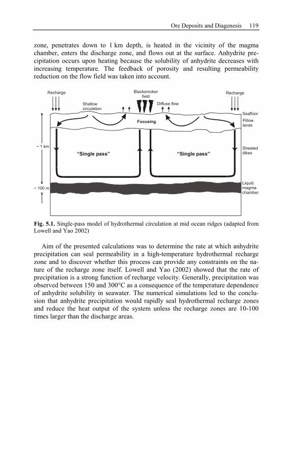
Ore Deposits and Diagenesis 119
zone, penetrates down to 1 km depth, is heated in the vicinity of the magma
chamber, enters the discharge zone, and flows out at the surface. Anhydrite pre-
cipitation occurs upon heating because the solubility of anhydrite decreases with
increasing temperature. The feedback of porosity and resulting permeability
reduction on the flow field was taken into account.
~ 1 km
~ 100 m
Blacksmoker
field
Recharge Recharge
Diffuse flowShallow
circulation
Focusing
“Single pass” “Single pass”
Seafloor
Pillow
lavas
Sheeted
dikes
Liquid
magma
chamber
Fig. 5.1. Single-pass model of hydrothermal circulation at mid ocean ridges (adapted from
Lowell and Yao 2002)
Aim of the presented calculations was to determine the rate at which anhydrite
precipitation can seal permeability in a high-temperature hydrothermal recharge
zone and to discover whether this process can provide any constraints on the na-
ture of the recharge zone itself. Lowell and Yao (2002) showed that the rate of
precipitation is a strong function of recharge velocity. Generally, precipitation was
observed between 150 and 300°C as a consequence of the temperature dependence
of anhydrite solubility in seawater. The numerical simulations led to the conclu-
sion that anhydrite precipitation would rapidly seal hydrothermal recharge zones
and reduce the heat output of the system unless the recharge zones are 10-100
times larger than the discharge areas.
120 Fossil Hydrothermal Systems
5.2 Anhydrite Cementation at the Location Allermöhe
It was planned to install a Geothermal Heating Station (GHS) at the location Al-
lermöhe (South-East of Hamburg, Germany) for district heating supply. The target
aquifer for water recovery has been the Rhaetkeuper, which feeds the GHS Neus-
tadt-Glewe (100 km east of Hamburg) with up to 120 m3 per hour since 1995. For
that reason, the bore Allermöhe 1 was deepened to a depth of 3,300 m in 1997. It
taps a 70 m thick sandstone aquifer with a temperature of 125°C. Although tem-
perature and thickness of the aquifer agree with the conditions needed for geo-
thermal energy use, the pore spaces, originally open with porosities up to 20 %,
are filled to a large extent by anhydrite. Mineralogical investigations showed ce-
mentation of secondary anhydrite with completely filled pore spaces as well as in-
sular, cloudy, or layered structures. The extractable amount of water, 3 m3 h
-1, de-
termined by a pumping test in 1998, is too low for an economical use of the
resource (Baermann et al., 2000a).
The intention of the numerical studies done here with the simulator SHEMAT
is to confirm or disprove the hypotheses for anhydrite cementation due to:
• Transport of solutes from neighboring salt structures into the Rhaetian sand-
stone and subsequent anhydrite precipitation (Lenz et al. 1997) studied here
under special consideration of the recent structure of the Allermöhe site and its
palaeogeological development, or
• up-flow of brines from deeper stratigraphic units via fault zones and resulting
anhydrite precipitation due to changing physical and chemical conditions
(Baermann et al. 2000a).
The findings provided by the numerical investigations are finally compared in dis-
cussion with two further attempts of explanation for the observed anhydrite ce-
mentation:
• Up-flow of brines from the underlying Gipsmergelkeuper formation and pre-
cipitation of anhydrite in the Rhaetian sandstone. Christensen et al. (2002)
stated that deposition is due to significant pressure differences of the neighbor-
ing geologic formations, and
• synsedimentary formation and growth of anhydrite due to capillary evaporation
in a highly saline and high temperature sabkha environment due to the arid cli-
mate of German Triassic times (Wurster 1965).
5.2.1 Geological Setting and History of the Salt Structures
The investigated site is located SE of Hamburg (Germany) between 53°24’-
53°30’N and 10°00’-10°10’E (Fig. 5.2). The study area is concurrent with part no.
2526 of the geological map of Hamburg scale 1:25000 (Sheet Allermöhe, Ehlers
1993). The Allermöhe well has been drilled at the position 53°28'N and 10°06'E in
the center of the NE quadrant of the map sheet (Fig. 5.2).
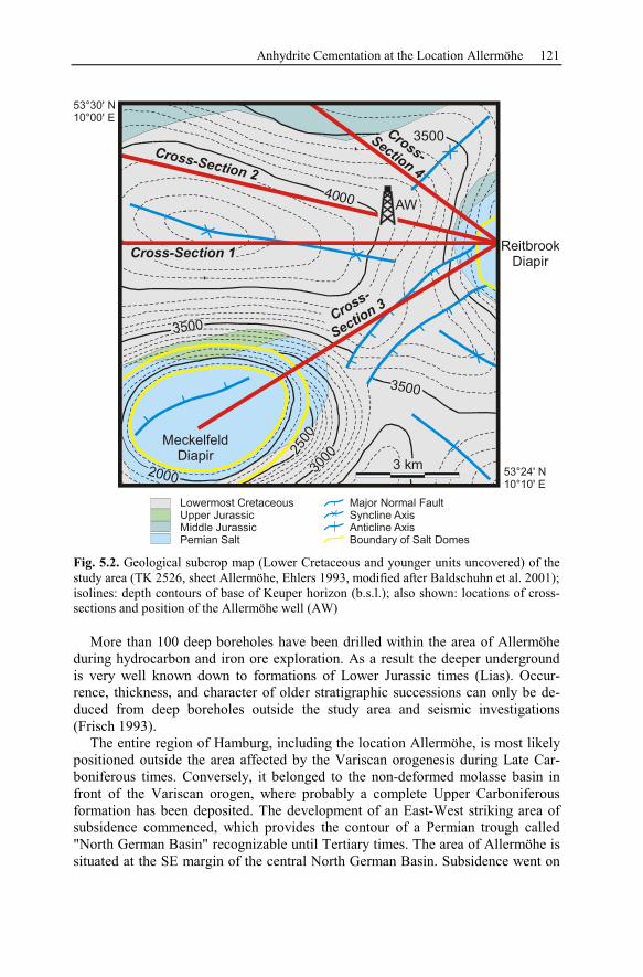
Anhydrite Cementation at the Location Allermöhe 121
4000
3500
3500
30002
500
2000
3500
Meckelfeld
Diapir
AW
Cross-Section 1
Cross-Section 2
Cross-
Section
3
Cross-
Section
4
Reitbrook
Diapir
53°30' N
10°00' E
53°24' N
10°10' E
Lowermost Cretaceous
Upper Jurassic
Middle Jurassic
Pemian Salt
Major Normal Fault
Syncline Axis
Anticline Axis
Boundary of Salt Domes
3 km
Fig. 5.2. Geological subcrop map (Lower Cretaceous and younger units uncovered) of the
study area (TK 2526, sheet Allermöhe, Ehlers 1993, modified after Baldschuhn et al. 2001);
isolines: depth contours of base of Keuper horizon (b.s.l.); also shown: locations of cross-
sections and position of the Allermöhe well (AW)
More than 100 deep boreholes have been drilled within the area of Allermöhe
during hydrocarbon and iron ore exploration. As a result the deeper underground
is very well known down to formations of Lower Jurassic times (Lias). Occur-
rence, thickness, and character of older stratigraphic successions can only be de-
duced from deep boreholes outside the study area and seismic investigations
(Frisch 1993).
The entire region of Hamburg, including the location Allermöhe, is most likely
positioned outside the area affected by the Variscan orogenesis during Late Car-
boniferous times. Conversely, it belonged to the non-deformed molasse basin in
front of the Variscan orogen, where probably a complete Upper Carboniferous
formation has been deposited. The development of an East-West striking area of
subsidence commenced, which provides the contour of a Permian trough called
"North German Basin" recognizable until Tertiary times. The area of Allermöhe is
situated at the SE margin of the central North German Basin. Subsidence went on
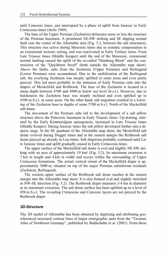
122 Fossil Hydrothermal Systems
until Cenozoic times, just interrupted by a phase of uplift from Jurassic to Early
Cretaceous times (Jaritz 1969).
The base of the Upper Permian (Zechstein) delineates more or less the structure
of the Permian basement. A prominent NE-SW striking and SE dipping normal
fault cuts the center of the Allermöhe area (Fig. 5.2, between the salt structures).
This structure was active during Mesozoic times due to isostatic compensation in
an extensional tectonic setting, and was reactivated in Early Tertiary times. From
Late Triassic times (Middle Keuper) until the end of the Mesozoic, extensional
normal faulting caused the uplift of the so-called "Hamburg Block" and the con-
struction of the "Quickborn Swell" (both outside the Allermöhe map sheet).
Above the faults, salts from the Zechstein (Upper Permian) and Rotliegend
(Lower Permian) were accumulated. Due to the mobilization of the Rotliegend
salt, the overlying Zechstein was steeply uplifted in some areas and even partly
pierced. This led most probably to the intrusion of Early Permian salts into the
diapirs of Meckelfeld and Reitbrook. The base of the Zechstein is located in a
mean depth between 4700 and 4900 m below sea level (b.s.l.). However, due to
halokinesis the Zechstein base was steeply inclined and even uplifted up to
4300 m b.s.l. in some areas. On the other hand, salt migration resulted in a lower-
ing of the Zechstein base to depths of some 5700 m b.s.l. North of the Meckelfeld
salt dome.
The movement of the Permian salts led to the development of a salt pillow
structure above the Paleozoic basement in Early Triassic times. Up-doming, initi-
ated by the Early Kimmeridgian epirogenesis, increased in Late Triassic times
(Middle Keuper). During Jurassic times the salt pillow developed further into a di-
apiric stage. In the SE quadrant of the Allermöhe map sheet, the Meckelfeld salt
dome evolved during Dogger times and at the eastern margin the Reitbrook salt
dome pierced up already in Lias times. Salt diapirism probably continued until La-
te Jurassic times and uplift gradually ceased in Early Cretaceous times.
The upper surface of the Meckelfeld salt dome is oval and slightly NE-SW stri-
king with an area of approximately 19 km² (Fig. 5.2). Its maximum extension is
7 km in length and 4 km in width and occurs within the surrounding of Upper
Cretaceous formations. The actual vertical extent of the Meckelfeld diapir is ap-
proximately 3000 m, situated on top of the major Permian saliniferous residuals
(Zechstein, Rotliegend).
The western upper surface of the Reitbrook salt dome reaches at the eastern
margin into the Allermöhe map sheet. It is also formed oval and slightly stretched
in NW-SE direction (Fig. 5.2). The Reitbrook diapir measures 3-4 km in diameter
at its maximum extension. The salt dome surface has been uplifted up to a level of
850 m b.s.l. The revealing Cretaceous and Cenozoic layers are not pierced by the
Reitbrook diapir.
3D-Structure
The 3D model of Allermöhe has been obtained by digitizing and attributing geo-
referenced structural contour lines of major stratigraphic units from the “Tectonic
Atlas of Northwest Germany“, published by Baldschuhn et al. (2001). From these
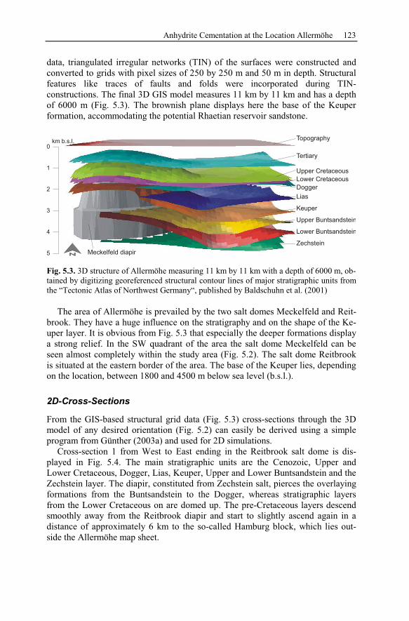
Anhydrite Cementation at the Location Allermöhe 123
data, triangulated irregular networks (TIN) of the surfaces were constructed and
converted to grids with pixel sizes of 250 by 250 m and 50 m in depth. Structural
features like traces of faults and folds were incorporated during TIN-
constructions. The final 3D GIS model measures 11 km by 11 km and has a depth
of 6000 m (Fig. 5.3). The brownish plane displays here the base of the Keuper
formation, accommodating the potential Rhaetian reservoir sandstone.
Topography
Tertiary
Upper Cretaceous
Lower Cretaceous
Dogger
Lias
Keuper
Upper Buntsandstein
Lower Buntsandstein
Zechstein
Meckelfeld diapir
0
1
2
3
4
5
km b.s.l.
Fig. 5.3. 3D structure of Allermöhe measuring 11 km by 11 km with a depth of 6000 m, ob-
tained by digitizing georeferenced structural contour lines of major stratigraphic units from
the “Tectonic Atlas of Northwest Germany“, published by Baldschuhn et al. (2001)
The area of Allermöhe is prevailed by the two salt domes Meckelfeld and Reit-
brook. They have a huge influence on the stratigraphy and on the shape of the Ke-
uper layer. It is obvious from Fig. 5.3 that especially the deeper formations display
a strong relief. In the SW quadrant of the area the salt dome Meckelfeld can be
seen almost completely within the study area (Fig. 5.2). The salt dome Reitbrook
is situated at the eastern border of the area. The base of the Keuper lies, depending
on the location, between 1800 and 4500 m below sea level (b.s.l.).
2D-Cross-Sections
From the GIS-based structural grid data (Fig. 5.3) cross-sections through the 3D
model of any desired orientation (Fig. 5.2) can easily be derived using a simple
program from Günther (2003a) and used for 2D simulations.
Cross-section 1 from West to East ending in the Reitbrook salt dome is dis-
played in Fig. 5.4. The main stratigraphic units are the Cenozoic, Upper and
Lower Cretaceous, Dogger, Lias, Keuper, Upper and Lower Buntsandstein and the
Zechstein layer. The diapir, constituted from Zechstein salt, pierces the overlaying
formations from the Buntsandstein to the Dogger, whereas stratigraphic layers
from the Lower Cretaceous on are domed up. The pre-Cretaceous layers descend
smoothly away from the Reitbrook diapir and start to slightly ascend again in a
distance of approximately 6 km to the so-called Hamburg block, which lies out-
side the Allermöhe map sheet.
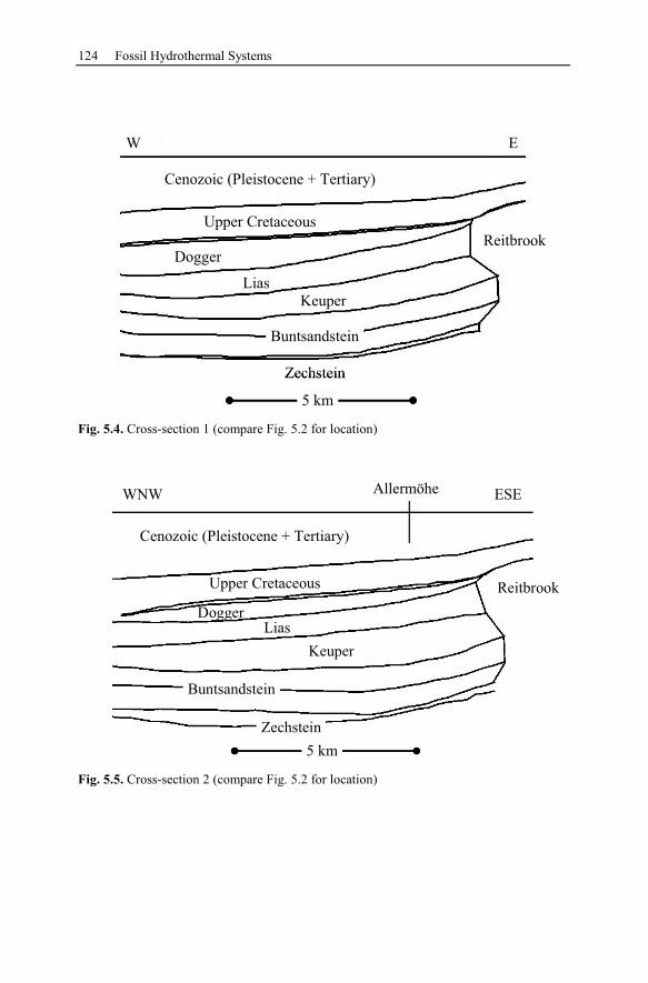
124 Fossil Hydrothermal Systems
Cenozoic (Pleistocene + Tertiary)
Upper Cretaceous
Reitbrook
Zechstein
Dogger
Lias
Keuper
Buntsandstein
5 km
W E
Cenozoic (Pleistocene + Tertiary)
Upper Cretaceous
Reitbrook
Zechstein
Dogger
Lias
Keuper
Buntsandstein
5 km5 km
W E
Fig. 5.4. Cross-section 1 (compare Fig. 5.2 for location)
Cenozoic (Pleistocene + Tertiary)
Upper Cretaceous Reitbrook
Zechstein
Dogger
Lias
Keuper
Buntsandstein
5 km
WNW ESEAllermöhe
Cenozoic (Pleistocene + Tertiary)
Upper Cretaceous Reitbrook
Zechstein
Dogger
Lias
Keuper
Buntsandstein
5 km
WNW ESEAllermöhe
Fig. 5.5. Cross-section 2 (compare Fig. 5.2 for location)
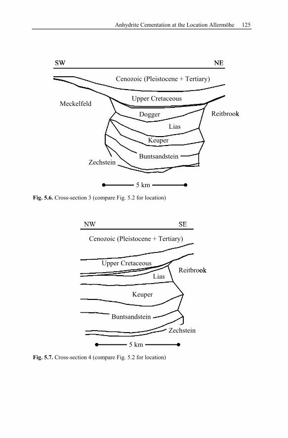
Anhydrite Cementation at the Location Allermöhe 125
Cenozoic (Pleistocene + Tertiary)
Upper Cretaceous
Reitbrook
Zechstein
Dogger
Lias
Keuper
Buntsandstein
Meckelfeld
5 km
SW NE
Cenozoic (Pleistocene + Tertiary)
Upper Cretaceous
Reitbrook
Zechstein
Dogger
Lias
Keuper
Buntsandstein
Meckelfeld
5 km5 km
SW NE
Fig. 5.6. Cross-section 3 (compare Fig. 5.2 for location)
Cenozoic (Pleistocene + Tertiary)
Upper Cretaceous
Reitbrook
Zechstein
Lias
Keuper
Buntsandstein
5 km
NW SE
Cenozoic (Pleistocene + Tertiary)
Upper Cretaceous
Reitbrook
Zechstein
Lias
Keuper
Buntsandstein
5 km5 km
NW SE
Fig. 5.7. Cross-section 4 (compare Fig. 5.2 for location)
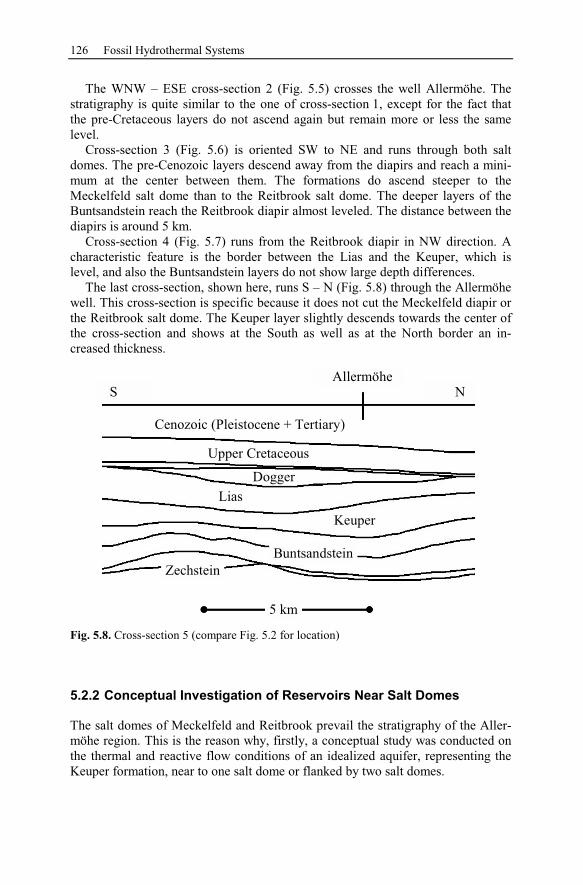
126 Fossil Hydrothermal Systems
The WNW – ESE cross-section 2 (Fig. 5.5) crosses the well Allermöhe. The
stratigraphy is quite similar to the one of cross-section 1, except for the fact that
the pre-Cretaceous layers do not ascend again but remain more or less the same
level.
Cross-section 3 (Fig. 5.6) is oriented SW to NE and runs through both salt
domes. The pre-Cenozoic layers descend away from the diapirs and reach a mini-
mum at the center between them. The formations do ascend steeper to the
Meckelfeld salt dome than to the Reitbrook salt dome. The deeper layers of the
Buntsandstein reach the Reitbrook diapir almost leveled. The distance between the
diapirs is around 5 km.
Cross-section 4 (Fig. 5.7) runs from the Reitbrook diapir in NW direction. A
characteristic feature is the border between the Lias and the Keuper, which is
level, and also the Buntsandstein layers do not show large depth differences.
The last cross-section, shown here, runs S – N (Fig. 5.8) through the Allermöhe
well. This cross-section is specific because it does not cut the Meckelfeld diapir or
the Reitbrook salt dome. The Keuper layer slightly descends towards the center of
the cross-section and shows at the South as well as at the North border an in-
creased thickness.
Cenozoic (Pleistocene + Tertiary)
Upper Cretaceous
Zechstein
Dogger
Lias
Keuper
Buntsandstein
5 km
S N
Allermöhe
Cenozoic (Pleistocene + Tertiary)
Upper Cretaceous
Zechstein
Dogger
Lias
Keuper
Buntsandstein
5 km5 km
S N
Allermöhe
Fig. 5.8. Cross-section 5 (compare Fig. 5.2 for location)
5.2.2 Conceptual Investigation of Reservoirs Near Salt Domes
The salt domes of Meckelfeld and Reitbrook prevail the stratigraphy of the Aller-
möhe region. This is the reason why, firstly, a conceptual study was conducted on
the thermal and reactive flow conditions of an idealized aquifer, representing the
Keuper formation, near to one salt dome or flanked by two salt domes.
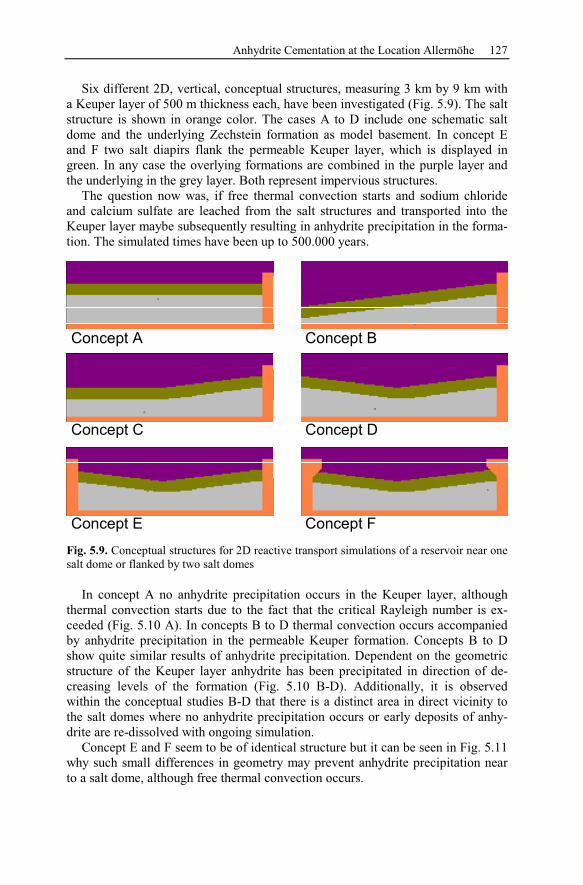
Anhydrite Cementation at the Location Allermöhe 127
Six different 2D, vertical, conceptual structures, measuring 3 km by 9 km with
a Keuper layer of 500 m thickness each, have been investigated (Fig. 5.9). The salt
structure is shown in orange color. The cases A to D include one schematic salt
dome and the underlying Zechstein formation as model basement. In concept E
and F two salt diapirs flank the permeable Keuper layer, which is displayed in
green. In any case the overlying formations are combined in the purple layer and
the underlying in the grey layer. Both represent impervious structures.
The question now was, if free thermal convection starts and sodium chloride
and calcium sulfate are leached from the salt structures and transported into the
Keuper layer maybe subsequently resulting in anhydrite precipitation in the forma-
tion. The simulated times have been up to 500.000 years.
Concept A Concept B
Concept C Concept D
Concept E Concept F
Fig. 5.9. Conceptual structures for 2D reactive transport simulations of a reservoir near one
salt dome or flanked by two salt domes
In concept A no anhydrite precipitation occurs in the Keuper layer, although
thermal convection starts due to the fact that the critical Rayleigh number is ex-
ceeded (Fig. 5.10 A). In concepts B to D thermal convection occurs accompanied
by anhydrite precipitation in the permeable Keuper formation. Concepts B to D
show quite similar results of anhydrite precipitation. Dependent on the geometric
structure of the Keuper layer anhydrite has been precipitated in direction of de-
creasing levels of the formation (Fig. 5.10 B-D). Additionally, it is observed
within the conceptual studies B-D that there is a distinct area in direct vicinity to
the salt domes where no anhydrite precipitation occurs or early deposits of anhy-
drite are re-dissolved with ongoing simulation.
Concept E and F seem to be of identical structure but it can be seen in Fig. 5.11
why such small differences in geometry may prevent anhydrite precipitation near
to a salt dome, although free thermal convection occurs.
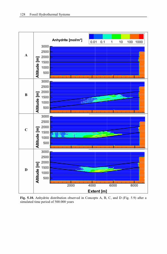
128 Fossil Hydrothermal Systems
A
Alt
itu
de
[m]
500
1000
1500
2000
2500
3000
0.01 0.1 1 10 100 1000Anhydrite [mol/m³]
B
Altitu
de
[m]
500
1000
1500
2000
2500
3000
C
Altitu
de
[m]
500
1000
1500
2000
2500
3000
D
Extent [m]
Altitu
de
[m]
2000 4000 6000 8000
500
1000
1500
2000
2500
3000
Fig. 5.10. Anhydrite distribution observed in Concepts A, B, C, and D (Fig. 5.9) after a
simulated time period of 500.000 years
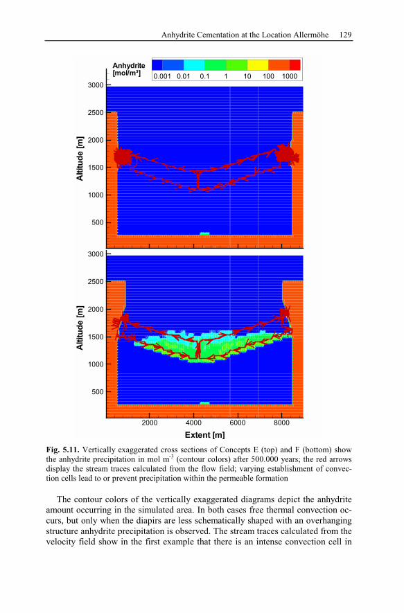
Anhydrite Cementation at the Location Allermöhe 129
Altitu
de
[m]
500
1000
1500
2000
2500
3000
0.001 0.01 0.1 1 10 100 1000
Anhydrite
[mol/m³]
Extent [m]
Altitu
de
[m]
2000 4000 6000 8000
500
1000
1500
2000
2500
3000
Fig. 5.11. Vertically exaggerated cross sections of Concepts E (top) and F (bottom) show
the anhydrite precipitation in mol m-3
(contour colors) after 500.000 years; the red arrows
display the stream traces calculated from the flow field; varying establishment of convec-
tion cells lead to or prevent precipitation within the permeable formation
The contour colors of the vertically exaggerated diagrams depict the anhydrite
amount occurring in the simulated area. In both cases free thermal convection oc-
curs, but only when the diapirs are less schematically shaped with an overhanging
structure anhydrite precipitation is observed. The stream traces calculated from the
velocity field show in the first example that there is an intense convection cell in
130 Fossil Hydrothermal Systems
direct vicinity to each salt dome. Additionally two greater convection cells exist
reaching down to the deepest level of the permeable Keuper layer. Away from the
diapirs flow occurs at the base of the aquifer and towards the salt structures at the
top of the layer. The stream traces of the second example show only the bigger
convection cells leading directly from the diapirs down the formation and up
again. The small convection cells near to the salt domes do not occur in this case.
Detailed investigation revealed higher horizontal flow rates for Concept F com-
pared to Concept E, resulting in mixed convection. Mixed convection takes place
when horizontal flows are superimposed on thermally driven flows. Convection
cells migrating laterally in the direction of horizontal flow characterize mixed
convection (Raffensberger and Vlassopoulus 1999).
It can be concluded that the development of one large flow structure due to lat-
erally migrating convection cells is necessary for the occurrence of solute trans-
port over larger distances into the formation. If a small convection cell exists near
to the salt dome all solutes are instantaneously back-transported to the salt struc-
ture. The difference in both examples solely consists in a small variation of the
diapir’s geometry.
To reach anhydrite cementation to an extent as observed in the Allermöhe well
within the described conceptual models (500 m permeable Keuper reservoir) a
minimum time period of around 150 Mio years would be necessary. This simpli-
fied assumption holds for the case that the feedback of reaction on the flow can be
neglected. Hence, precipitation or dissolution within the pore space structure does
not change the flow field and flow velocities.
5.2.3 Geological History of the Recent Structure of Allermöhe
The importance of the structural geometry, mentioned before, on anhydrite trans-
port processes led to the investigation of historical geological sequences (both in
2D and 3D). Simulations were carried out in order to determine the occurrence of
thermal convection and resulting anhydrite precipitation dependent on the struc-
tural geometry in certain geological time-intervals. The set up of the 2D sequence
is based on data of Schmitz and Flixeder (1993). Source for the 3D sequence is the
structural model of the study area (Fig. 5.3).
2D Restoration Sequence
Schmitz and Flixeder (1993) published a roughly WNW-ESE striking 2D vertical
cross-section through the Reitbrook diapir. The Reitbrook diapir is of special im-
portance for the Allermöhe well due to its proximity. Their cross section was used
to firstly make a sketch of the recent structure (Fig. 5.12). The 2D cross section
shows the stratigraphy from Cenozoic down to Rotliegend units of the area around
the Allermöhe well and the Reitbrook diapir.
The recent structure of the location Allermöhe (Fig. 5.12) is evolved backwards
to Keuper times based on the actual, original, available geologic data. The work
has been done applying a structural modeling algorithm to analyze the subsidence
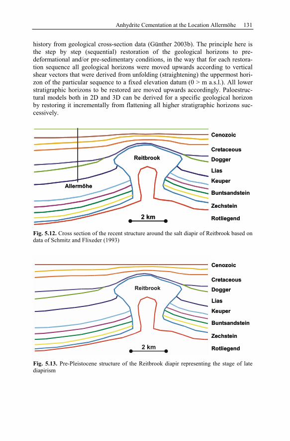
Anhydrite Cementation at the Location Allermöhe 131
history from geological cross-section data (Günther 2003b). The principle here is
the step by step (sequential) restoration of the geological horizons to pre-
deformational and/or pre-sedimentary conditions, in the way that for each restora-
tion sequence all geological horizons were moved upwards according to vertical
shear vectors that were derived from unfolding (straightening) the uppermost hori-
zon of the particular sequence to a fixed elevation datum (0 > m a.s.l.). All lower
stratigraphic horizons to be restored are moved upwards accordingly. Paloestruc-
tural models both in 2D and 3D can be derived for a specific geological horizon
by restoring it incrementally from flattening all higher stratigraphic horizons suc-
cessively.
Allermöhe
2 km
Keuper
Lias
Dogger
Cretaceous
Buntsandstein
Cenozoic
Zechstein
Rotliegend
Reitbrook
Allermöhe
2 km
Keuper
Lias
Dogger
Cretaceous
Buntsandstein
Cenozoic
Zechstein
Rotliegend
Reitbrook
Fig. 5.12. Cross section of the recent structure around the salt diapir of Reitbrook based on
data of Schmitz and Flixeder (1993)
Keuper
Lias
Dogger
Cretaceous
Buntsandstein
Cenozoic
Zechstein
Rotliegend
Reitbrook
2 km
Keuper
Lias
Dogger
Cretaceous
Buntsandstein
Cenozoic
Zechstein
Rotliegend
Reitbrook
2 km
Fig. 5.13. Pre-Pleistocene structure of the Reitbrook diapir representing the stage of late
diapirism
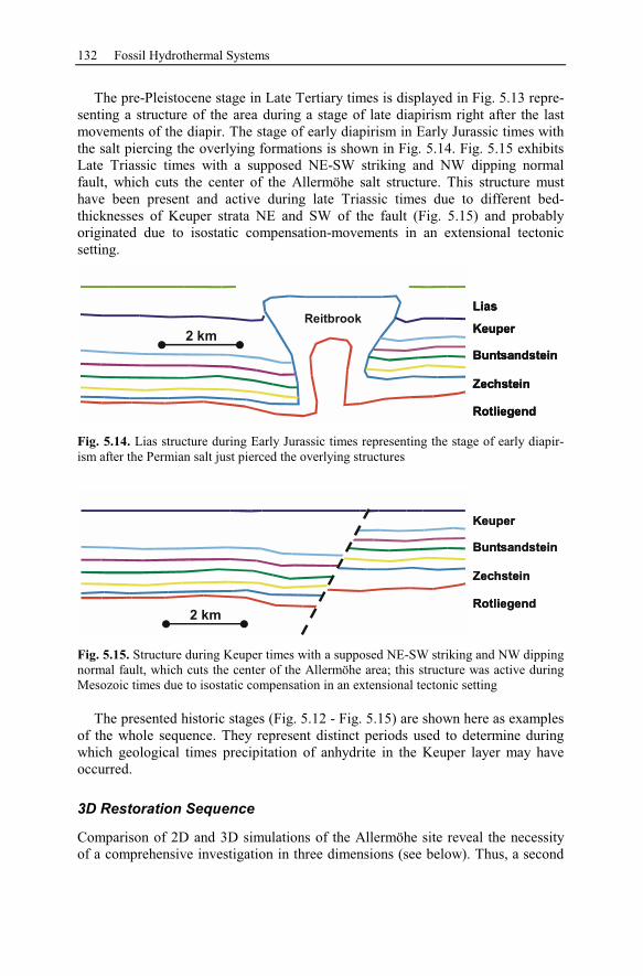
132 Fossil Hydrothermal Systems
The pre-Pleistocene stage in Late Tertiary times is displayed in Fig. 5.13 repre-
senting a structure of the area during a stage of late diapirism right after the last
movements of the diapir. The stage of early diapirism in Early Jurassic times with
the salt piercing the overlying formations is shown in Fig. 5.14. Fig. 5.15 exhibits
Late Triassic times with a supposed NE-SW striking and NW dipping normal
fault, which cuts the center of the Allermöhe salt structure. This structure must
have been present and active during late Triassic times due to different bed-
thicknesses of Keuper strata NE and SW of the fault (Fig. 5.15) and probably
originated due to isostatic compensation-movements in an extensional tectonic
setting.
Keuper
Lias
Buntsandstein
Zechstein
Rotliegend
2 km
ReitbrookKeuper
Lias
Buntsandstein
Zechstein
Rotliegend
Keuper
Lias
Buntsandstein
Zechstein
Rotliegend
2 km
Reitbrook
Fig. 5.14. Lias structure during Early Jurassic times representing the stage of early diapir-
ism after the Permian salt just pierced the overlying structures
Keuper
Buntsandstein
Zechstein
Rotliegend
2 km
Keuper
Buntsandstein
Zechstein
Rotliegend
2 km
Fig. 5.15. Structure during Keuper times with a supposed NE-SW striking and NW dipping
normal fault, which cuts the center of the Allermöhe area; this structure was active during
Mesozoic times due to isostatic compensation in an extensional tectonic setting
The presented historic stages (Fig. 5.12 - Fig. 5.15) are shown here as examples
of the whole sequence. They represent distinct periods used to determine during
which geological times precipitation of anhydrite in the Keuper layer may have
occurred.
3D Restoration Sequence
Comparison of 2D and 3D simulations of the Allermöhe site reveal the necessity
of a comprehensive investigation in three dimensions (see below). Thus, a second
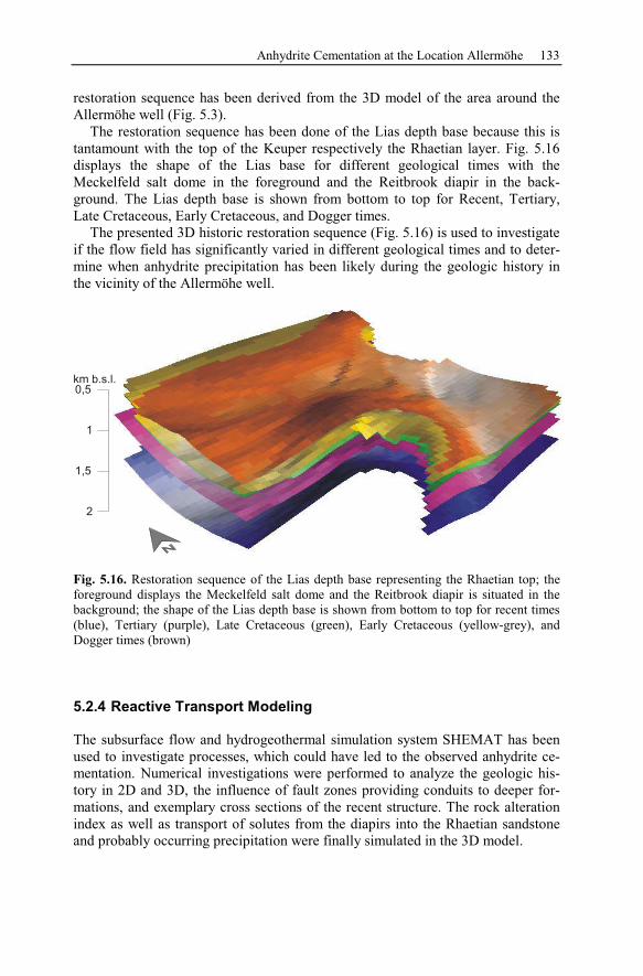
Anhydrite Cementation at the Location Allermöhe 133
restoration sequence has been derived from the 3D model of the area around the
Allermöhe well (Fig. 5.3).
The restoration sequence has been done of the Lias depth base because this is
tantamount with the top of the Keuper respectively the Rhaetian layer. Fig. 5.16
displays the shape of the Lias base for different geological times with the
Meckelfeld salt dome in the foreground and the Reitbrook diapir in the back-
ground. The Lias depth base is shown from bottom to top for Recent, Tertiary,
Late Cretaceous, Early Cretaceous, and Dogger times.
The presented 3D historic restoration sequence (Fig. 5.16) is used to investigate
if the flow field has significantly varied in different geological times and to deter-
mine when anhydrite precipitation has been likely during the geologic history in
the vicinity of the Allermöhe well.
0,5
1
1,5
2
km b.s.l.
Fig. 5.16. Restoration sequence of the Lias depth base representing the Rhaetian top; the
foreground displays the Meckelfeld salt dome and the Reitbrook diapir is situated in the
background; the shape of the Lias depth base is shown from bottom to top for recent times
(blue), Tertiary (purple), Late Cretaceous (green), Early Cretaceous (yellow-grey), and
Dogger times (brown)
5.2.4 Reactive Transport Modeling
The subsurface flow and hydrogeothermal simulation system SHEMAT has been
used to investigate processes, which could have led to the observed anhydrite ce-
mentation. Numerical investigations were performed to analyze the geologic his-
tory in 2D and 3D, the influence of fault zones providing conduits to deeper for-
mations, and exemplary cross sections of the recent structure. The rock alteration
index as well as transport of solutes from the diapirs into the Rhaetian sandstone
and probably occurring precipitation were finally simulated in the 3D model.
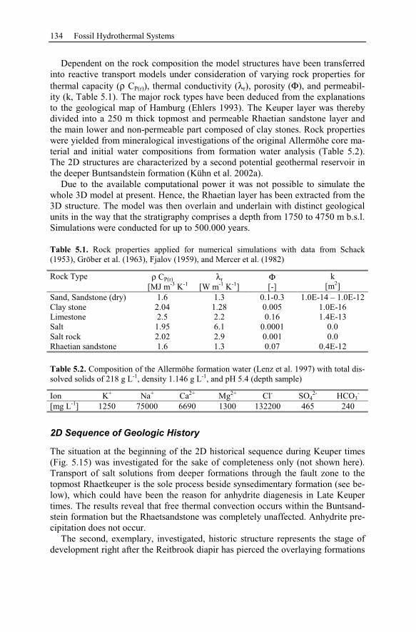
134 Fossil Hydrothermal Systems
Dependent on the rock composition the model structures have been transferred
into reactive transport models under consideration of varying rock properties for
thermal capacity (ρ CP(r)), thermal conductivity (λr), porosity (Φ), and permeabil-
ity (k, Table 5.1). The major rock types have been deduced from the explanations
to the geological map of Hamburg (Ehlers 1993). The Keuper layer was thereby
divided into a 250 m thick topmost and permeable Rhaetian sandstone layer and
the main lower and non-permeable part composed of clay stones. Rock properties
were yielded from mineralogical investigations of the original Allermöhe core ma-
terial and initial water compositions from formation water analysis (Table 5.2).
The 2D structures are characterized by a second potential geothermal reservoir in
the deeper Buntsandstein formation (Kühn et al. 2002a).
Due to the available computational power it was not possible to simulate the
whole 3D model at present. Hence, the Rhaetian layer has been extracted from the
3D structure. The model was then overlain and underlain with distinct geological
units in the way that the stratigraphy comprises a depth from 1750 to 4750 m b.s.l.
Simulations were conducted for up to 500.000 years.
Table 5.1. Rock properties applied for numerical simulations with data from Schack
(1953), Gröber et al. (1963), Fjalov (1959), and Mercer et al. (1982)
Rock Type ρ CP(r)
[MJ m-3
K-1
λr
[W m-1
K-1
]
Φ[-]
k
[m2]
Sand, Sandstone (dry) 1.6 1.3 0.1-0.3 1.0E-14 – 1.0E-12
Clay stone 2.04 1.28 0.005 1.0E-16
Limestone 2.5 2.2 0.16 1.4E-13
Salt 1.95 6.1 0.0001 0.0
Salt rock 2.02 2.9 0.001 0.0
Rhaetian sandstone 1.6 1.3 0.07 0.4E-12
Table 5.2. Composition of the Allermöhe formation water (Lenz et al. 1997) with total dis-
solved solids of 218 g L-1
, density 1.146 g L-1
, and pH 5.4 (depth sample)
Ion K+ Na
+ Ca
2+ Mg
2+ Cl
- SO4
2- HCO3
-
[mg L-1
] 1250 75000 6690 1300 132200 465 240
2D Sequence of Geologic History
The situation at the beginning of the 2D historical sequence during Keuper times
(Fig. 5.15) was investigated for the sake of completeness only (not shown here).
Transport of salt solutions from deeper formations through the fault zone to the
topmost Rhaetkeuper is the sole process beside synsedimentary formation (see be-
low), which could have been the reason for anhydrite diagenesis in Late Keuper
times. The results reveal that free thermal convection occurs within the Buntsand-
stein formation but the Rhaetsandstone was completely unaffected. Anhydrite pre-
cipitation does not occur.
The second, exemplary, investigated, historic structure represents the stage of
development right after the Reitbrook diapir has pierced the overlaying formations
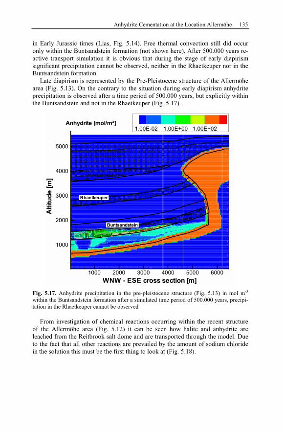
Anhydrite Cementation at the Location Allermöhe 135
in Early Jurassic times (Lias, Fig. 5.14). Free thermal convection still did occur
only within the Buntsandstein formation (not shown here). After 500.000 years re-
active transport simulation it is obvious that during the stage of early diapirism
significant precipitation cannot be observed, neither in the Rhaetkeuper nor in the
Buntsandstein formation.
Late diapirism is represented by the Pre-Pleistocene structure of the Allermöhe
area (Fig. 5.13). On the contrary to the situation during early diapirism anhydrite
precipitation is observed after a time period of 500.000 years, but explicitly within
the Buntsandstein and not in the Rhaetkeuper (Fig. 5.17).
WNW - ESE cross section [m]
Altitu
de
[m]
1000 2000 3000 4000 5000 6000
1000
2000
3000
4000
5000
1.00E-02 1.00E+00 1.00E+02
Anhydrite [mol/m³]
Buntsandstein
Rhaetkeuper
Fig. 5.17. Anhydrite precipitation in the pre-pleistocene structure (Fig. 5.13) in mol m-3
within the Buntsandstein formation after a simulated time period of 500.000 years, precipi-
tation in the Rhaetkeuper cannot be observed
From investigation of chemical reactions occurring within the recent structure
of the Allermöhe area (Fig. 5.12) it can be seen how halite and anhydrite are
leached from the Reitbrook salt dome and are transported through the model. Due
to the fact that all other reactions are prevailed by the amount of sodium chloride
in the solution this must be the first thing to look at (Fig. 5.18).
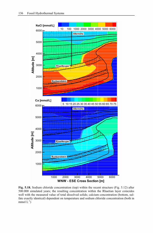
136 Fossil Hydrothermal Systems
Altitu
de
[m]
1000
2000
3000
4000
5000
600010 100 1000 2000 3000 4000 5000 6000
NaCl [mmol/L]
Buntsandstein
Allermöhe
Rhaetkeuper
WNW - ESE Cross Section [m]
Altitu
de
[m]
1000 2000 3000 4000 5000 6000
1000
2000
3000
4000
5000
60005 10 15 20 25 30 35 40 45 50 55 60 65 70 75
Ca [mmol/L]
Allermöhe
Rhaetkeuper
Buntsandstein
Fig. 5.18. Sodium chloride concentration (top) within the recent structure (Fig. 5.12) after
500.000 simulated years; the resulting concentration within the Rhaetian layer coincides
well with the measured value of total dissolved solids; calcium concentration (bottom, sul-
fate exactly identical) dependent on temperature and sodium chloride concentration (both in
mmol L-1
)
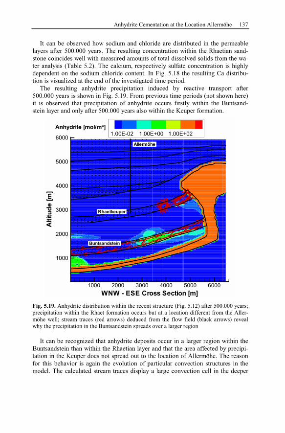
Anhydrite Cementation at the Location Allermöhe 137
It can be observed how sodium and chloride are distributed in the permeable
layers after 500.000 years. The resulting concentration within the Rhaetian sand-
stone coincides well with measured amounts of total dissolved solids from the wa-
ter analysis (Table 5.2). The calcium, respectively sulfate concentration is highly
dependent on the sodium chloride content. In Fig. 5.18 the resulting Ca distribu-
tion is visualized at the end of the investigated time period.
The resulting anhydrite precipitation induced by reactive transport after
500.000 years is shown in Fig. 5.19. From previous time periods (not shown here)
it is observed that precipitation of anhydrite occurs firstly within the Buntsand-
stein layer and only after 500.000 years also within the Keuper formation.
WNW - ESE Cross Section [m]
Alt
itu
de
[m]
1000 2000 3000 4000 5000 6000
1000
2000
3000
4000
5000
60001.00E-02 1.00E+00 1.00E+02
Anhydrite [mol/m³]
Allermöhe
Rhaetkeuper
Buntsandstein
Fig. 5.19. Anhydrite distribution within the recent structure (Fig. 5.12) after 500.000 years;
precipitation within the Rhaet formation occurs but at a location different from the Aller-
möhe well; stream traces (red arrows) deduced from the flow field (black arrows) reveal
why the precipitation in the Buntsandstein spreads over a larger region
It can be recognized that anhydrite deposits occur in a larger region within the
Buntsandstein than within the Rhaetian layer and that the area affected by precipi-
tation in the Keuper does not spread out to the location of Allermöhe. The reason
for this behavior is again the evolution of particular convection structures in the
model. The calculated stream traces display a large convection cell in the deeper
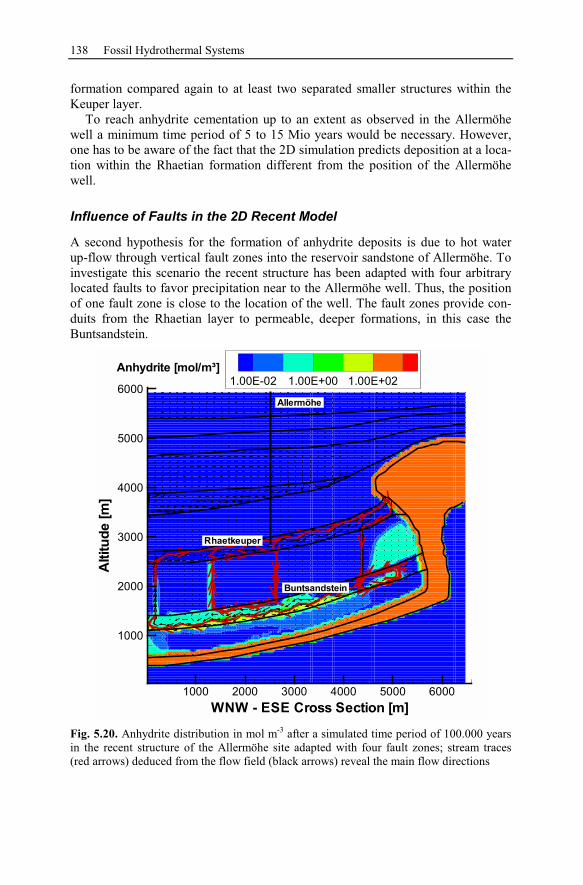
138 Fossil Hydrothermal Systems
formation compared again to at least two separated smaller structures within the
Keuper layer.
To reach anhydrite cementation up to an extent as observed in the Allermöhe
well a minimum time period of 5 to 15 Mio years would be necessary. However,
one has to be aware of the fact that the 2D simulation predicts deposition at a loca-
tion within the Rhaetian formation different from the position of the Allermöhe
well.
Influence of Faults in the 2D Recent Model
A second hypothesis for the formation of anhydrite deposits is due to hot water
up-flow through vertical fault zones into the reservoir sandstone of Allermöhe. To
investigate this scenario the recent structure has been adapted with four arbitrary
located faults to favor precipitation near to the Allermöhe well. Thus, the position
of one fault zone is close to the location of the well. The fault zones provide con-
duits from the Rhaetian layer to permeable, deeper formations, in this case the
Buntsandstein.
WNW - ESE Cross Section [m]
Altitu
de
[m]
1000 2000 3000 4000 5000 6000
1000
2000
3000
4000
5000
60001.00E-02 1.00E+00 1.00E+02
Anhydrite [mol/m³]
Allermöhe
Rhaetkeuper
Buntsandstein
Fig. 5.20. Anhydrite distribution in mol m-3
after a simulated time period of 100.000 years
in the recent structure of the Allermöhe site adapted with four fault zones; stream traces
(red arrows) deduced from the flow field (black arrows) reveal the main flow directions
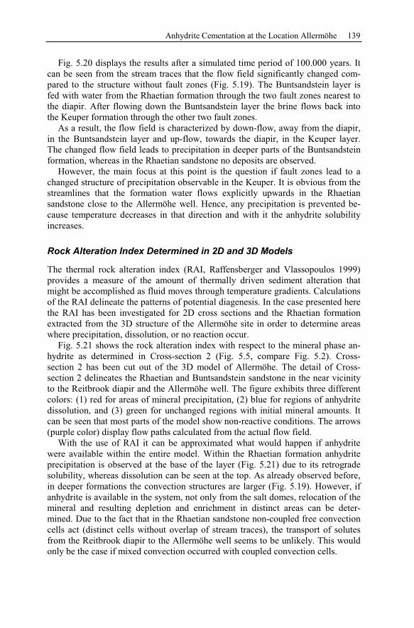
Anhydrite Cementation at the Location Allermöhe 139
Fig. 5.20 displays the results after a simulated time period of 100.000 years. It
can be seen from the stream traces that the flow field significantly changed com-
pared to the structure without fault zones (Fig. 5.19). The Buntsandstein layer is
fed with water from the Rhaetian formation through the two fault zones nearest to
the diapir. After flowing down the Buntsandstein layer the brine flows back into
the Keuper formation through the other two fault zones.
As a result, the flow field is characterized by down-flow, away from the diapir,
in the Buntsandstein layer and up-flow, towards the diapir, in the Keuper layer.
The changed flow field leads to precipitation in deeper parts of the Buntsandstein
formation, whereas in the Rhaetian sandstone no deposits are observed.
However, the main focus at this point is the question if fault zones lead to a
changed structure of precipitation observable in the Keuper. It is obvious from the
streamlines that the formation water flows explicitly upwards in the Rhaetian
sandstone close to the Allermöhe well. Hence, any precipitation is prevented be-
cause temperature decreases in that direction and with it the anhydrite solubility
increases.
Rock Alteration Index Determined in 2D and 3D Models
The thermal rock alteration index (RAI, Raffensberger and Vlassopoulos 1999)
provides a measure of the amount of thermally driven sediment alteration that
might be accomplished as fluid moves through temperature gradients. Calculations
of the RAI delineate the patterns of potential diagenesis. In the case presented here
the RAI has been investigated for 2D cross sections and the Rhaetian formation
extracted from the 3D structure of the Allermöhe site in order to determine areas
where precipitation, dissolution, or no reaction occur.
Fig. 5.21 shows the rock alteration index with respect to the mineral phase an-
hydrite as determined in Cross-section 2 (Fig. 5.5, compare Fig. 5.2). Cross-
section 2 has been cut out of the 3D model of Allermöhe. The detail of Cross-
section 2 delineates the Rhaetian and Buntsandstein sandstone in the near vicinity
to the Reitbrook diapir and the Allermöhe well. The figure exhibits three different
colors: (1) red for areas of mineral precipitation, (2) blue for regions of anhydrite
dissolution, and (3) green for unchanged regions with initial mineral amounts. It
can be seen that most parts of the model show non-reactive conditions. The arrows
(purple color) display flow paths calculated from the actual flow field.
With the use of RAI it can be approximated what would happen if anhydrite
were available within the entire model. Within the Rhaetian formation anhydrite
precipitation is observed at the base of the layer (Fig. 5.21) due to its retrograde
solubility, whereas dissolution can be seen at the top. As already observed before,
in deeper formations the convection structures are larger (Fig. 5.19). However, if
anhydrite is available in the system, not only from the salt domes, relocation of the
mineral and resulting depletion and enrichment in distinct areas can be deter-
mined. Due to the fact that in the Rhaetian sandstone non-coupled free convection
cells act (distinct cells without overlap of stream traces), the transport of solutes
from the Reitbrook diapir to the Allermöhe well seems to be unlikely. This would
only be the case if mixed convection occurred with coupled convection cells.
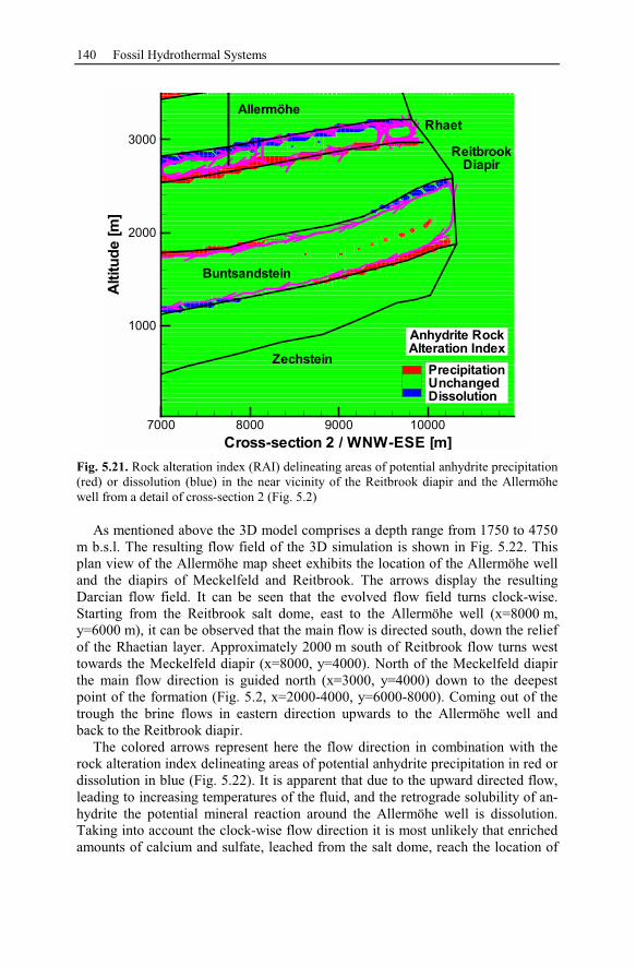
140 Fossil Hydrothermal Systems
Cross-section 2 / WNW-ESE [m]
Altitu
de
[m]
7000 8000 9000 10000
1000
2000
3000
105
95
Anhydrite Rock
Alteration Index
Precipitation
Unchanged
Dissolution
Reitbrook
Diapir
Allermöhe
Rhaet
Buntsandstein
Zechstein
Fig. 5.21. Rock alteration index (RAI) delineating areas of potential anhydrite precipitation
(red) or dissolution (blue) in the near vicinity of the Reitbrook diapir and the Allermöhe
well from a detail of cross-section 2 (Fig. 5.2)
As mentioned above the 3D model comprises a depth range from 1750 to 4750
m b.s.l. The resulting flow field of the 3D simulation is shown in Fig. 5.22. This
plan view of the Allermöhe map sheet exhibits the location of the Allermöhe well
and the diapirs of Meckelfeld and Reitbrook. The arrows display the resulting
Darcian flow field. It can be seen that the evolved flow field turns clock-wise.
Starting from the Reitbrook salt dome, east to the Allermöhe well (x=8000 m,
y=6000 m), it can be observed that the main flow is directed south, down the relief
of the Rhaetian layer. Approximately 2000 m south of Reitbrook flow turns west
towards the Meckelfeld diapir (x=8000, y=4000). North of the Meckelfeld diapir
the main flow direction is guided north (x=3000, y=4000) down to the deepest
point of the formation (Fig. 5.2, x=2000-4000, y=6000-8000). Coming out of the
trough the brine flows in eastern direction upwards to the Allermöhe well and
back to the Reitbrook diapir.
The colored arrows represent here the flow direction in combination with the
rock alteration index delineating areas of potential anhydrite precipitation in red or
dissolution in blue (Fig. 5.22). It is apparent that due to the upward directed flow,
leading to increasing temperatures of the fluid, and the retrograde solubility of an-
hydrite the potential mineral reaction around the Allermöhe well is dissolution.
Taking into account the clock-wise flow direction it is most unlikely that enriched
amounts of calcium and sulfate, leached from the salt dome, reach the location of
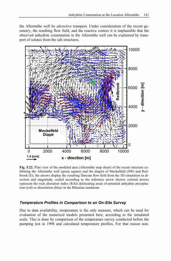
Anhydrite Cementation at the Location Allermöhe 141
the Allermöhe well by advective transport. Under consideration of the recent ge-
ometry, the resulting flow field, and the reactive centers it is implausible that the
observed anhydrite cementation in the Allermöhe well can be explained by trans-
port of solutes from the salt structures.
0
2000
4000
6000
8000
10000
y-
dir
ectio
n[m
]
0 2000 4000 6000 8000 10000
x - direction [m]1.0 [m/a]
Meckelfeld
Diapir
Re
itb
roo
k
Fig. 5.22. Plan view of the modeled area (Allermöhe map sheet) of the recent structure ex-
hibiting the Allermöhe well (green square) and the diapirs of Meckelfeld (SW) and Reit-
brook (E); the arrows display the resulting Darcian flow field from the 3D simulation in di-
rection and magnitude, scaled according to the reference arrow shown; colored arrows
represent the rock alteration index (RAI) delineating areas of potential anhydrite precipita-
tion (red) or dissolution (blue) in the Rhaetian sandstone
Temperature Profiles in Comparison to an On-Site Survey
Due to data availability, temperature is the only measure, which can be used for
evaluation of the numerical models presented here, according to the simulated
scale. This is done by comparison of the temperature survey conducted before the
pumping test in 1998 and calculated temperature profiles. For that reason non-
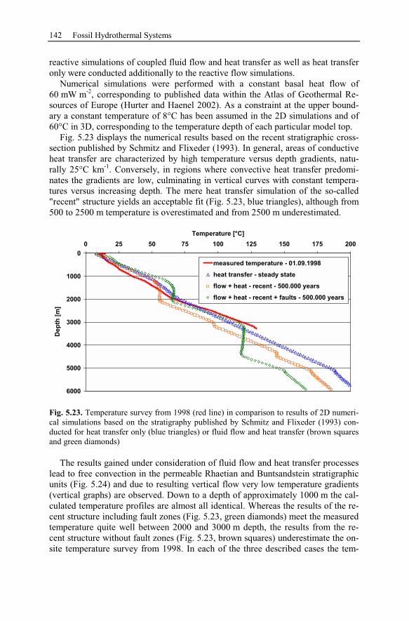
142 Fossil Hydrothermal Systems
reactive simulations of coupled fluid flow and heat transfer as well as heat transfer
only were conducted additionally to the reactive flow simulations.
Numerical simulations were performed with a constant basal heat flow of
60 mW m-2
, corresponding to published data within the Atlas of Geothermal Re-
sources of Europe (Hurter and Haenel 2002). As a constraint at the upper bound-
ary a constant temperature of 8°C has been assumed in the 2D simulations and of
60°C in 3D, corresponding to the temperature depth of each particular model top.
Fig. 5.23 displays the numerical results based on the recent stratigraphic cross-
section published by Schmitz and Flixeder (1993). In general, areas of conductive
heat transfer are characterized by high temperature versus depth gradients, natu-
rally 25°C km-1
. Conversely, in regions where convective heat transfer predomi-
nates the gradients are low, culminating in vertical curves with constant tempera-
tures versus increasing depth. The mere heat transfer simulation of the so-called
"recent" structure yields an acceptable fit (Fig. 5.23, blue triangles), although from
500 to 2500 m temperature is overestimated and from 2500 m underestimated.
0
1000
2000
3000
4000
5000
6000
0 25 50 75 100 125 150 175 200
Temperature [°C]
Dep
th [
m]
measured temperature - 01.09.1998
heat transfer - steady state
flow + heat - recent - 500.000 years
flow + heat - recent + faults - 500.000 years
Fig. 5.23. Temperature survey from 1998 (red line) in comparison to results of 2D numeri-
cal simulations based on the stratigraphy published by Schmitz and Flixeder (1993) con-
ducted for heat transfer only (blue triangles) or fluid flow and heat transfer (brown squares
and green diamonds)
The results gained under consideration of fluid flow and heat transfer processes
lead to free convection in the permeable Rhaetian and Buntsandstein stratigraphic
units (Fig. 5.24) and due to resulting vertical flow very low temperature gradients
(vertical graphs) are observed. Down to a depth of approximately 1000 m the cal-
culated temperature profiles are almost all identical. Whereas the results of the re-
cent structure including fault zones (Fig. 5.23, green diamonds) meet the measured
temperature quite well between 2000 and 3000 m depth, the results from the re-
cent structure without fault zones (Fig. 5.23, brown squares) underestimate the on-
site temperature survey from 1998. In each of the three described cases the tem-
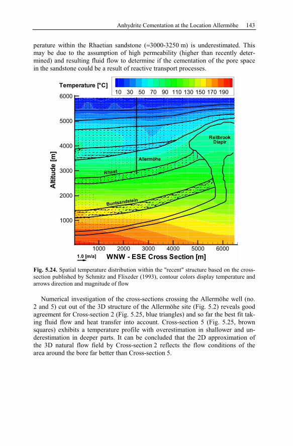
Anhydrite Cementation at the Location Allermöhe 143
perature within the Rhaetian sandstone (≈3000-3250 m) is underestimated. This
may be due to the assumption of high permeability (higher than recently deter-
mined) and resulting fluid flow to determine if the cementation of the pore space
in the sandstone could be a result of reactive transport processes.
WNW - ESE Cross Section [m]
Altitu
de
[m]
1000 2000 3000 4000 5000 6000
1000
2000
3000
4000
5000
600010 30 50 70 90 110 130 150 170 190
Temperature [°C]
1.0 [m/a]
Reitbrook
Diapir
Allermöhe
Rhaet
Buntsandstein
Fig. 5.24. Spatial temperature distribution within the "recent" structure based on the cross-
section published by Schmitz and Flixeder (1993), contour colors display temperature and
arrows direction and magnitude of flow
Numerical investigation of the cross-sections crossing the Allermöhe well (no.
2 and 5) cut out of the 3D structure of the Allermöhe site (Fig. 5.2) reveals good
agreement for Cross-section 2 (Fig. 5.25, blue triangles) and so far the best fit tak-
ing fluid flow and heat transfer into account. Cross-section 5 (Fig. 5.25, brown
squares) exhibits a temperature profile with overestimation in shallower and un-
derestimation in deeper parts. It can be concluded that the 2D approximation of
the 3D natural flow field by Cross-section 2 reflects the flow conditions of the
area around the bore far better than Cross-section 5.
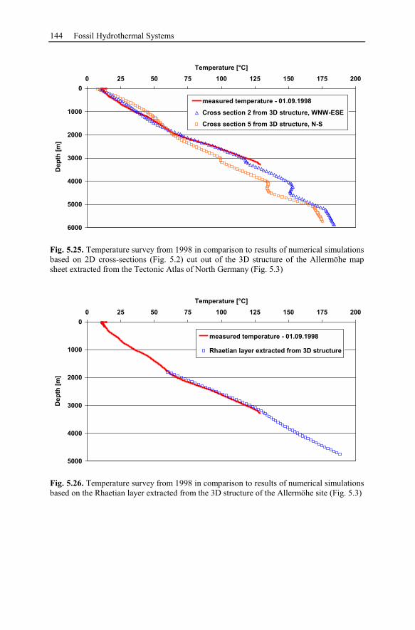
144 Fossil Hydrothermal Systems
0
1000
2000
3000
4000
5000
6000
0 25 50 75 100 125 150 175 200
Temperature [°C]
Dep
th [
m]
measured temperature - 01.09.1998
Cross section 2 from 3D structure, WNW-ESE
Cross section 5 from 3D structure, N-S
Fig. 5.25. Temperature survey from 1998 in comparison to results of numerical simulations
based on 2D cross-sections (Fig. 5.2) cut out of the 3D structure of the Allermöhe map
sheet extracted from the Tectonic Atlas of North Germany (Fig. 5.3)
0
1000
2000
3000
4000
5000
0 25 50 75 100 125 150 175 200
Temperature [°C]
Dep
th [
m]
measured temperature - 01.09.1998
Rhaetian layer extracted from 3D structure
Fig. 5.26. Temperature survey from 1998 in comparison to results of numerical simulations
based on the Rhaetian layer extracted from the 3D structure of the Allermöhe site (Fig. 5.3)
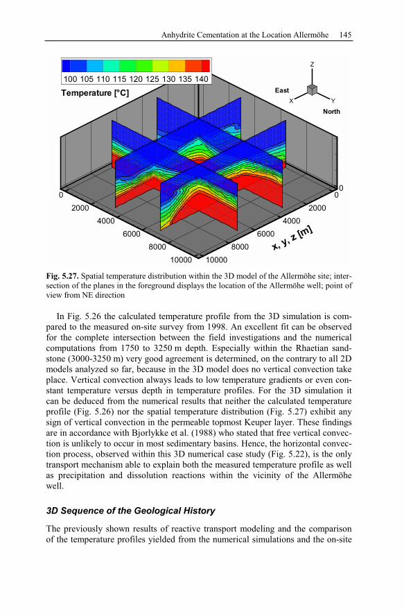
Anhydrite Cementation at the Location Allermöhe 145
00
2000
4000
6000
8000
10000
x, y, z [m]
0
2000
4000
6000
8000
10000
X Y
Z
100 105 110 115 120 125 130 135 140
Temperature [°C]
North
East
Fig. 5.27. Spatial temperature distribution within the 3D model of the Allermöhe site; inter-
section of the planes in the foreground displays the location of the Allermöhe well; point of
view from NE direction
In Fig. 5.26 the calculated temperature profile from the 3D simulation is com-
pared to the measured on-site survey from 1998. An excellent fit can be observed
for the complete intersection between the field investigations and the numerical
computations from 1750 to 3250 m depth. Especially within the Rhaetian sand-
stone (3000-3250 m) very good agreement is determined, on the contrary to all 2D
models analyzed so far, because in the 3D model does no vertical convection take
place. Vertical convection always leads to low temperature gradients or even con-
stant temperature versus depth in temperature profiles. For the 3D simulation it
can be deduced from the numerical results that neither the calculated temperature
profile (Fig. 5.26) nor the spatial temperature distribution (Fig. 5.27) exhibit any
sign of vertical convection in the permeable topmost Keuper layer. These findings
are in accordance with Bjorlykke et al. (1988) who stated that free vertical convec-
tion is unlikely to occur in most sedimentary basins. Hence, the horizontal convec-
tion process, observed within this 3D numerical case study (Fig. 5.22), is the only
transport mechanism able to explain both the measured temperature profile as well
as precipitation and dissolution reactions within the vicinity of the Allermöhe
well.
3D Sequence of the Geological History
The previously shown results of reactive transport modeling and the comparison
of the temperature profiles yielded from the numerical simulations and the on-site
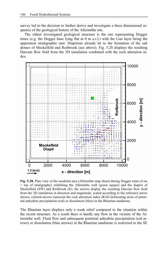
146 Fossil Hydrothermal Systems
survey led to the decision to further derive and investigate a three dimensional se-
quence of the geological history of the Allermöhe site.
The oldest investigated geological structure is the one representing Dogger
times (e.g. the Dogger base lying flat at 0 m a.s.l.) with the Lias layer being the
uppermost stratigraphic unit. Diapirism already let to the formation of the salt
domes of Meckelfeld and Reitbrook (see above). Fig. 5.28 displays the resulting
Darcian flow field from the 3D simulation combined with the rock alteration in-
dex.
0
2000
4000
6000
8000
10000
y-
dir
ectio
n[m
]
0 2000 4000 6000 8000 10000
x - direction [m]1.0 [m/a]
Meckelfeld
Diapir
Re
itb
roo
k
Fig. 5.28. Plan view of the modeled area (Allermöhe map sheet) during Dogger times (Lias
= top of stratigraphy) exhibiting the Allermöhe well (green square) and the diapirs of
Meckelfeld (SW) and Reitbrook (E); the arrows display the resulting Darcian flow field
from the 3D simulation in direction and magnitude, scaled according to the reference arrow
shown; colored arrows represent the rock alteration index (RAI) delineating areas of poten-
tial anhydrite precipitation (red) or dissolution (blue) in the Rhaetian sandstone
The Rhaetian layer displays only a weak relief compared to the situation within
the recent structure. As a result there is hardly any flow in the vicinity of the Al-
lermöhe well. Fluid flow and subsequent potential anhydrite precipitation (red ar-
rows) or dissolution (blue arrows) in the Rhaetian sandstone is restricted to the SE
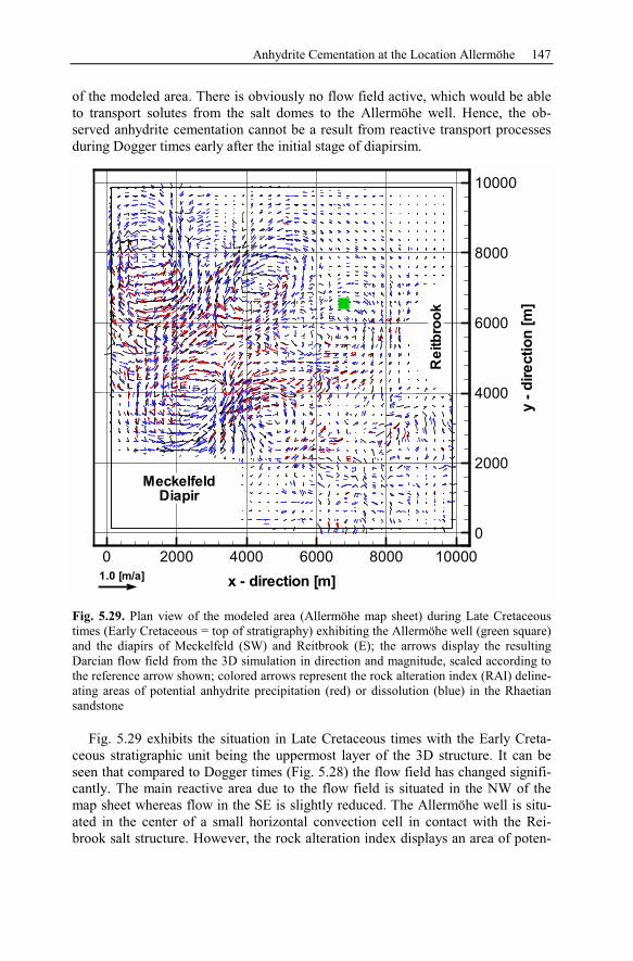
Anhydrite Cementation at the Location Allermöhe 147
of the modeled area. There is obviously no flow field active, which would be able
to transport solutes from the salt domes to the Allermöhe well. Hence, the ob-
served anhydrite cementation cannot be a result from reactive transport processes
during Dogger times early after the initial stage of diapirsim.
0
2000
4000
6000
8000
10000
y-
dir
ectio
n[m
]
0 2000 4000 6000 8000 10000
x - direction [m]1.0 [m/a]
Meckelfeld
Diapir
Re
itb
roo
k
Fig. 5.29. Plan view of the modeled area (Allermöhe map sheet) during Late Cretaceous
times (Early Cretaceous = top of stratigraphy) exhibiting the Allermöhe well (green square)
and the diapirs of Meckelfeld (SW) and Reitbrook (E); the arrows display the resulting
Darcian flow field from the 3D simulation in direction and magnitude, scaled according to
the reference arrow shown; colored arrows represent the rock alteration index (RAI) deline-
ating areas of potential anhydrite precipitation (red) or dissolution (blue) in the Rhaetian
sandstone
Fig. 5.29 exhibits the situation in Late Cretaceous times with the Early Creta-
ceous stratigraphic unit being the uppermost layer of the 3D structure. It can be
seen that compared to Dogger times (Fig. 5.28) the flow field has changed signifi-
cantly. The main reactive area due to the flow field is situated in the NW of the
map sheet whereas flow in the SE is slightly reduced. The Allermöhe well is situ-
ated in the center of a small horizontal convection cell in contact with the Rei-
brook salt structure. However, the rock alteration index displays an area of poten-
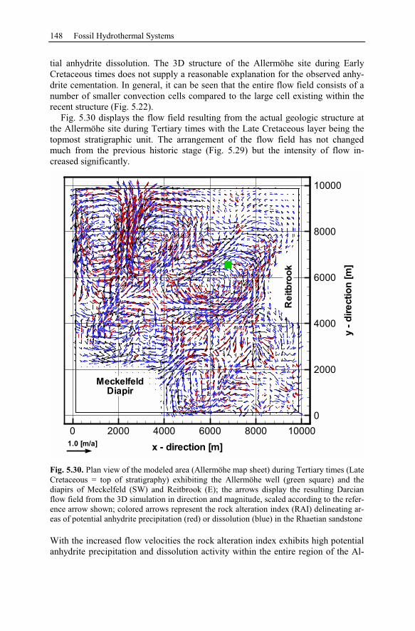
148 Fossil Hydrothermal Systems
tial anhydrite dissolution. The 3D structure of the Allermöhe site during Early
Cretaceous times does not supply a reasonable explanation for the observed anhy-
drite cementation. In general, it can be seen that the entire flow field consists of a
number of smaller convection cells compared to the large cell existing within the
recent structure (Fig. 5.22).
Fig. 5.30 displays the flow field resulting from the actual geologic structure at
the Allermöhe site during Tertiary times with the Late Cretaceous layer being the
topmost stratigraphic unit. The arrangement of the flow field has not changed
much from the previous historic stage (Fig. 5.29) but the intensity of flow in-
creased significantly.
0
2000
4000
6000
8000
10000
y-
dir
ectio
n[m
]
0 2000 4000 6000 8000 10000
x - direction [m]1.0 [m/a]
Meckelfeld
Diapir
Re
itb
roo
k
Fig. 5.30. Plan view of the modeled area (Allermöhe map sheet) during Tertiary times (Late
Cretaceous = top of stratigraphy) exhibiting the Allermöhe well (green square) and the
diapirs of Meckelfeld (SW) and Reitbrook (E); the arrows display the resulting Darcian
flow field from the 3D simulation in direction and magnitude, scaled according to the refer-
ence arrow shown; colored arrows represent the rock alteration index (RAI) delineating ar-
eas of potential anhydrite precipitation (red) or dissolution (blue) in the Rhaetian sandstone
With the increased flow velocities the rock alteration index exhibits high potential
anhydrite precipitation and dissolution activity within the entire region of the Al-
Anhydrite Cementation at the Location Allermöhe 149
lermöhe map sheet. A clockwise convection cell still characterizes the vicinity of
the Allermöhe well. Dissolution of anhydrite is most likely around the well during
Tertiary times. In the NW quadrant a region with high flow rates and both anhy-
drite precipitation and dissolution can be seen. Detailed investigation reveals dis-
solution in shallower parts of the Rhaetian sandstone and precipitation in deeper
parts.
From the rock alteration index simulations of the 3D historical sequence, repre-
senting a measure for the degree of anhydrite relocation in the investigated area
during different geological times, it can be concluded that anhydrite precipitation
near to the Allermöhe well is most unlikely even when anhydrite is supplied by a
source different from the salt structures. The varying flow fields and rock altera-
tion indices (Fig. 5.22 and Fig. 5.28 - Fig. 5.30) emphasize an area of anhydrite
dissolution around the Allermöhe well. However, it is obvious that during all in-
vestigated geologic times, the development of horizontal convection cells leads to
specific anhydrite precipitation and dissolution pattern assuming that sufficient
amounts of anhydrite are available.
Transport of Solutes from the Salt Structures to the Allermöhe Well
Conversely to the investigation of the rock alteration index where anhydrite is
supplied from the entire investigated area (previous section), the reactive transport
simulation shown here starts with the assumption that anhydrite is available from
the salt structures only. The Rhaetian sandstone is initially assumed to be totally
free of anhydrite. The aim is to determine anhydrite precipitation patterns for the
entire area of the Allermöhe map sheet and to further investigate if precipitation of
anhydrite may occur at the Allermöhe well due to anhydrite dissolution from the
diapirs and transport of calcium and sulfate through the 3D structures.
Fig. 5.31 displays the resulting flow field within the recent structure of the Al-
lermöhe site after a simulated time period of 50,000 years. The red arrows display
areas with anhydrite amounts exceeding 10 mol m-3
, due to transport of solutes
from the salt structures and subsequent precipitation of anhydrite. It is obvious
that significant amounts of anhydrite do occur only in the southern parts of the in-
vestigated area but not around the Allermöhe well. This is due to the fact that the
large convection cell turns clockwise and the solutes, leached from the salt struc-
tures, firstly flow down to deeper and hotter parts of the 3D structure, resulting in
anhydrite precipitation. Flow towards the location of the Allermöhe well is di-
rected upwards the Rhaetian sandstone leading to increasing temperatures and
lowering the probability of precipitation.
Comparison of the observed precipitation patterns shown in Fig. 5.31 with the
RAI determined within the recent 3D structure (Fig. 5.22) reveals agreement of
the regions where anhydrite precipitation is simulated. From that point of view it
could be supposed that the RAI already provides complete information about re-
gions where precipitation occur and the areas where anhydrite deposits could be
excluded. For further examination of this hypothesis the other geological struc-
tures of the 3D historical restoration sequence (Fig. 5.28 - Fig. 5.30) were investi-
gated in the same manner. The leaching process from the salt structures followed
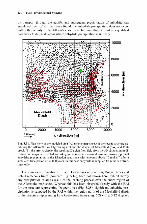
150 Fossil Hydrothermal Systems
by transport through the aquifer and subsequent precipitation of anhydrite was
simulated. First of all it has been found that anhydrite precipitation does not occur
within the vicinity of the Allermöhe well, emphasizing that the RAI is a qualified
parameter to delineate areas where anhydrite precipitation is unlikely.
0
2000
4000
6000
8000
10000
y-
dir
ectio
n[m
]
0 2000 4000 6000 8000 10000
x - direction [m]1.0 [m/a]
Meckelfeld
Diapir
Re
itb
roo
k
Fig. 5.31. Plan view of the modeled area (Allermöhe map sheet) of the recent structure ex-
hibiting the Allermöhe well (green square) and the diapirs of Meckelfeld (SW) and Reit-
brook (E); the arrows display the resulting Darcian flow field from the 3D simulation in di-
rection and magnitude, scaled according to the reference arrow shown; red arrows represent
anhydrite precipitation in the Rhaetian sandstone with amounts above 10 mol m-3
after a
simulated time period of 50,000 years; in this case anhydrite is supplied from the salt struc-
tures only
The numerical simulations of the 3D structures representing Dogger times and
Late Cretaceous times (compare Fig. 5.16), both not shown here, exhibit hardly
any precipitation at all as result of the leaching process over the entire region of
the Allermöhe map sheet. Whereas this has been observed already with the RAI
for the structure representing Dogger times (Fig. 5.28), significant anhydrite pre-
cipitation is supposed by the RAI within the region north of the Meckelfeld diapir
in the structure representing Late Cretaceous times (Fig. 5.29). Fig. 5.32 displays
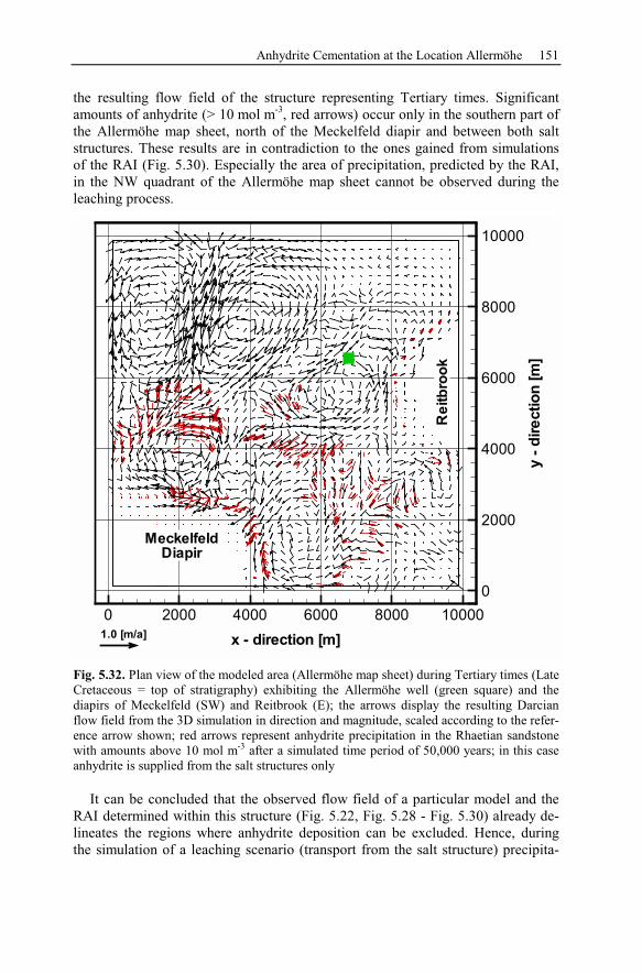
Anhydrite Cementation at the Location Allermöhe 151
the resulting flow field of the structure representing Tertiary times. Significant
amounts of anhydrite (> 10 mol m-3
, red arrows) occur only in the southern part of
the Allermöhe map sheet, north of the Meckelfeld diapir and between both salt
structures. These results are in contradiction to the ones gained from simulations
of the RAI (Fig. 5.30). Especially the area of precipitation, predicted by the RAI,
in the NW quadrant of the Allermöhe map sheet cannot be observed during the
leaching process.
0
2000
4000
6000
8000
10000
y-
dir
ectio
n[m
]
0 2000 4000 6000 8000 10000
x - direction [m]1.0 [m/a]
Meckelfeld
Diapir
Re
itb
roo
k
Fig. 5.32. Plan view of the modeled area (Allermöhe map sheet) during Tertiary times (Late
Cretaceous = top of stratigraphy) exhibiting the Allermöhe well (green square) and the
diapirs of Meckelfeld (SW) and Reitbrook (E); the arrows display the resulting Darcian
flow field from the 3D simulation in direction and magnitude, scaled according to the refer-
ence arrow shown; red arrows represent anhydrite precipitation in the Rhaetian sandstone
with amounts above 10 mol m-3
after a simulated time period of 50,000 years; in this case
anhydrite is supplied from the salt structures only
It can be concluded that the observed flow field of a particular model and the
RAI determined within this structure (Fig. 5.22, Fig. 5.28 - Fig. 5.30) already de-
lineates the regions where anhydrite deposition can be excluded. Hence, during
the simulation of a leaching scenario (transport from the salt structure) precipita-
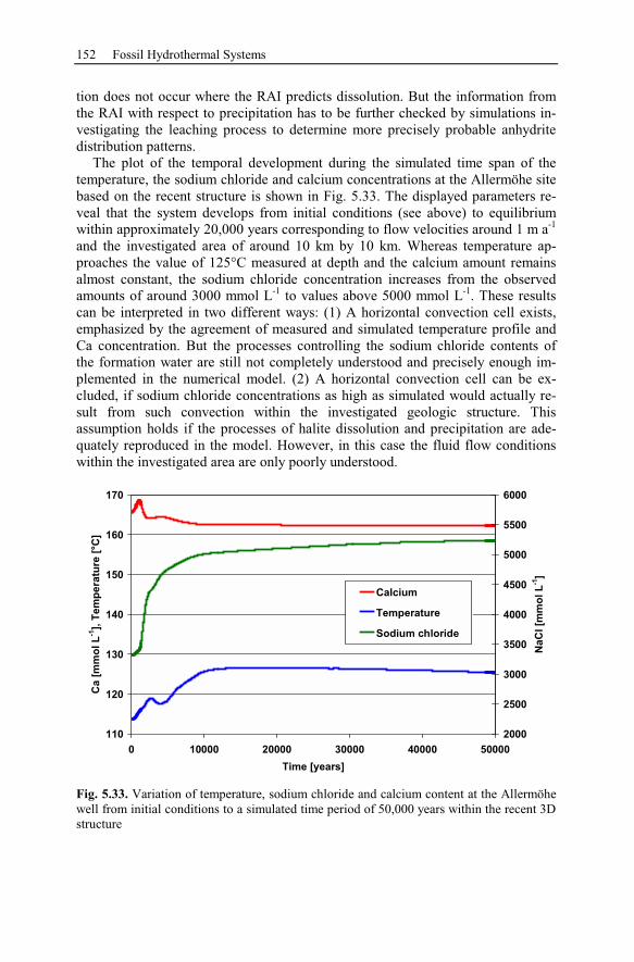
152 Fossil Hydrothermal Systems
tion does not occur where the RAI predicts dissolution. But the information from
the RAI with respect to precipitation has to be further checked by simulations in-
vestigating the leaching process to determine more precisely probable anhydrite
distribution patterns.
The plot of the temporal development during the simulated time span of the
temperature, the sodium chloride and calcium concentrations at the Allermöhe site
based on the recent structure is shown in Fig. 5.33. The displayed parameters re-
veal that the system develops from initial conditions (see above) to equilibrium
within approximately 20,000 years corresponding to flow velocities around 1 m a-1
and the investigated area of around 10 km by 10 km. Whereas temperature ap-
proaches the value of 125°C measured at depth and the calcium amount remains
almost constant, the sodium chloride concentration increases from the observed
amounts of around 3000 mmol L-1
to values above 5000 mmol L-1
. These results
can be interpreted in two different ways: (1) A horizontal convection cell exists,
emphasized by the agreement of measured and simulated temperature profile and
Ca concentration. But the processes controlling the sodium chloride contents of
the formation water are still not completely understood and precisely enough im-
plemented in the numerical model. (2) A horizontal convection cell can be ex-
cluded, if sodium chloride concentrations as high as simulated would actually re-
sult from such convection within the investigated geologic structure. This
assumption holds if the processes of halite dissolution and precipitation are ade-
quately reproduced in the model. However, in this case the fluid flow conditions
within the investigated area are only poorly understood.
110
120
130
140
150
160
170
0 10000 20000 30000 40000 50000
Time [years]
Ca [
mm
ol
L-1
], T
em
pe
ra
ture
[°C
]
2000
2500
3000
3500
4000
4500
5000
5500
6000
NaC
l [m
mo
l L
-1]
Calcium
Temperature
Sodium chloride
Fig. 5.33. Variation of temperature, sodium chloride and calcium content at the Allermöhe
well from initial conditions to a simulated time period of 50,000 years within the recent 3D
structure
Anhydrite Cementation at the Location Allermöhe 153
5.2.5 Summary and Conclusions of the Allermöhe Case Study
In sufficiently thick and permeable formations free thermal convection is a poten-
tial process for mass and heat transport and diagenesis in sedimentary basins
(Bjorlykke et al. 1988, Raffensberger and Garven 1995). A conceptual study was
performed under the assumption of a 500 m thick and permeable reservoir in the
vicinity to salt domes (Fig. 5.9). Free convection led to transport of solutes
leached from the salt diapirs and resulting precipitation of anhydrite in the forma-
tion. The 2D numerical simulations revealed that the occurrence of anhydrite de-
posits strongly depends on the geometry of the stratigraphic units (Fig. 5.11).
The relevance of the structural geometry for the Allermöhe site was investi-
gated by a 2D historical sequence (Fig. 5.12 - Fig. 5.15). However, the simulations
showed that only the geometry of the recent structure might cause anhydrite pre-
cipitation in the Rhaetian sandstone (Fig. 5.19). A minimum time period of 5 to 15
Mio years would be necessary to produce anhydrite cementation to an extent as
observed in the Allermöhe well. Nevertheless, the 2D simulation of the recent
structure predicts anhydrite to precipitate particularly outside the region where the
Allermöhe well is situated (Fig. 5.19). Even fault zones, providing conduits to
deeper formations, are not suitable to explain the reduction of porosity at the Al-
lermöhe site. On the contrary, the anhydrite precipitation observed in the Rhaetian
aquifer in the recent structure is prevented due to the flow field evolving as a re-
sult of the fault zones (Fig. 5.19 and Fig. 5.20).
The temperature survey from 1998 has been used to evaluate the results of the
numerical studies. Simulation of the 3D structure of the Rhaetian formation pro-
vides an excellent fit for the temperature profile with the on-site survey (Fig. 5.26)
conversely to the 2D calculations, which all exhibit especially within the Rhaetian
layer (3000-3250 m) disagreement with the measurements (Fig. 5.23, Fig. 5.25,
and Fig. 5.26). Flow field and temperature distribution emphasize that free hori-
zontal convection occurs, whereas vertical convection, as predicted within the 2D
models is most unlikely. Three-dimensional models are a prerequisite for an ade-
quate reproduction of fluid flow and heat transfer processes at the Allermöhe site.
The thermal rock alteration index (RAI, Raffensberger and Vlassopoulos 1999)
provides a measure of the amount of thermally driven sediment alteration due to
fluid movement. The simulations of the 3D historical restoration sequence of the
Allermöhe site reveal that the area around the Allermöhe well is only affected by
dissolution (Fig. 5.22, Fig. 5.28 - Fig. 5.30). The observed flow field of a particu-
lar model and the RAI determined within this structure already delineate the re-
gions where anhydrite deposition can be excluded. Hence, during the simulation
of a leaching scenario (transport from the salt structure, Fig. 5.31 and Fig. 5.32)
precipitation does not occur where the RAI predicts dissolution. But the informa-
tion from the RAI with respect to precipitation has to be further checked by simu-
lations investigating the leaching process to determine more precisely probable
anhydrite distribution patterns.
The conclusions which can be drawn from the presented numerical simulations,
studied here under special consideration of the geological structure of the Aller-
möhe site and its historical development falsifies the hypothesis of Lenz et al.
154 Fossil Hydrothermal Systems
(1997). Their assumption that the observed anhydrite cementation at the location
of the Allermöhe well may be due to solutes, leached from the salt structures,
transported through the system, and subsequently precipitated, is most unlikely.
Firstly, it has been shown that the geometry of areas in vicinity to salt structures is
highly important. Secondly, this led to the conclusion that 2D simulations of the
Allermöhe site are not able to represent flow field and temperature distribution ac-
curately. Distinct investigation of various palaeo 3D structures emphasized that
the vicinity of the Allermöhe well is a potential area of anhydrite dissolution and
that precipitation occurs predominantly in southern parts of the area. But even the
horizontal convection cells, observed within the 3D simulations, are questionable,
because the simulated temporal development of the sodium chloride concentration
at the Allermöhe well significantly deviates from chemical measurements (Fig.
5.33). Hence, transport of solutes from the diapirs to the Allermöhe well seems to
be implausible.
The hypothesis of Baermann et al. (2000a) that up-flow of brines from deeper
stratigraphic units via fault zones and resulting anhydrite precipitation due to
changing temperature and chemical conditions does not hold either. Although sig-
nificant changes of the flow field has been shown within the 2D simulations inves-
tigating the influence of fault zones, the up-flow always leads to decreasing tem-
peratures and a decreasing potential of anhydrite precipitation.
Christensen et al. (2002) also state that up-flow of brines may be the reason for
the observed anhydrite cementation at the Allermöhe site. They assume that solu-
tions from the Gipsmergelkeuper, underlying the Rhaetian sandstone formation,
led to precipitation of anhydrite due to significant pressure differences of the
neighboring geologic formations. Fact is, that the close neighborhood of Rhaet
and Gipsmergelkeuper excludes significant pressure differences for the case that
fault zones hydraulically connect both formations. Hence, the solubility difference
of anhydrite within the formation waters is small. Additionally, the analyzed sul-
fate isotopic signature of Allermöhe core samples is significantly different from
Keuper samples as published by Baermann et al. (2000b). If dissolution, transport,
and subsequent precipitation are the reason for an observed cementation the sul-
fate isotopic signature of source and target must be identical. Both arguments dis-
prove the theory of Christensen et al. (2002).
Major arguments have been presented that falsifies the hypotheses attributing
the anhydrite cementation observed at the Allermöhe site to the leaching of solutes
from salt diapirs or deeper stratigraphic units, their transport into the Rhaetian
sandstone, and subsequent precipitation of anhydrite. However, a mechanism suit-
able to explain the anhydrite formation within the Rhaetian sandstone at Aller-
möhe must be compatible on the one hand with the "regional scale" of the anhy-
drite cementation (meters to kilometers) and on the other hand with the structures
observed at the "well scale" (decimeter). Another hypothesis, the formation and
growth of anhydrite due to capillary evaporation in a highly saline and high tem-
perature sabkha environment (sabkha is an Arabic word for salt flat), not dis-
cussed so far, may provide a mechanism suitable to combine anhydrite distribution
patterns on all scales.
Anhydrite Cementation at the Location Allermöhe 155
Sabkhas are low-lying salt-encrusted marine or continental mudflats where dis-
placive and replacive evaporite minerals are forming in the capillary zone above a
saline water table (Warren 1989). Evaporites form where a potential exists for
more water to leave the basin by evaporation than to enter the basin by a combina-
tion of rainfall, surface, and subsurface inflow. Thus, evaporite deposits are most
often found in arid and semiarid deserts (ancient or recent). This is in agreement
with the arid climate stated by Wurster (1965) for the German Triassic times.
Characteristic environments thought to be important for the development of
sabkhas exhibit a continuous spectrum from marine coastal to fluviolacustrine and
eolian dominated types (Handford 1981). Sandstones of the Rhaetian in the area of
Hannover (gasfield Thönse, ≈150 km south of Allermöhe) were deposited in a
westward prograding fluvial-dominated delta. Lateral shifts of the delta position
are assumed to be responsible for sudden cessation of sand sedimentation. The ba-
sin wide sea level rise during the Rhaetian is expected to be the major reason for
the landward retrogradation of deltaic facies belts to the east (Gaupp 1991). It has
generally been observed that many ancient sabkhas evolved during a single pro-
gradational or retrogradational episode in the coastal plain from marine coastal to
eolian to fluviolacustrine-dominated systems or vice versa (Warren and Kendall
1985).
Most of the evaporites in a sabkha are deposited in the capillary zone as in-
trastratal nodules and crystals. Sabkhas form shoaling sequences in both continen-
tal and coastal mud flats. Idealized sabkha sequences are cycles with displacive
evaporites in the upper part of the salt flat. Each cycle is capped by an erosion sur-
face, the result of displacive crystal growth raising the surface of the wet mud flat
into the vadose zone. Prograding marine sabkhas exhibit gradation with finer ma-
terial to the top, while continental sabkhas tend to coarsen upward. Sandy reser-
voirs are found in marine sabkhas in the subtidal and intertidal sand bodies sealed
by evaporites. Sandy reservoirs in continental sabkhas reflect infilled stream
channels and dune sand sheets (Warren 1989). Mineralogical investigations of the
Rhaetian sandstone samples performed by Baermann et al. (2000a) showed com-
parable sequences of alternating layers of shale and sandstone, sandstone with in-
terbedded shale fillings, and massive bedded sandstones.
Many ancient evaporites are composed of salts originally formed by the con-
centration of seawater-derived brines. When the brine has about five times the
concentration of seawater (175 g L-1
total dissolved solids compared to 218 g L-1
of the Allermöhe formation water) gypsum precipitates. As the system is concen-
trated to a level slightly before halite saturation (eleven times seawater, 385 g L-1
),
anhydrite replaces gypsum. The calcium sulfate minerals gypsum and anhydrite
are important phases and their occurrences depend on prevailing temperature,
pressure, and salinities. Anhydrite can precipitate and grow by capillary evapora-
tion due to high salinities or temperature, or it can replace gypsum already present
in the sabkha. Hence, when bedded gypsum is buried and the temperature rises
above 60°C it is transformed to nodular anhydrite (Warren and Kendall 1985).
Baermann et al. (2000a) found similar patterns of anhydrite cementation in the Al-
lermöhe core samples: beside sandstone layers with pore spaces totally filled with
anhydrite, insular or cloudy, and layered anhydrite cementation were observed in
156 Fossil Hydrothermal Systems
cyclic sequences. Evaporites are susceptible to diagenesis from the time they are
first laid down, and this often destroys much of the early depositional textures. For
example, subsurface movement of pore waters can leach evaporites in siliclastic
matrices creating secondary porosity.
From the known facts, synsedimentary formation of the observed anhydrite
cementation is the most likely of all discussed hypotheses. Growth of anhydrite
due to capillary evaporation in a highly saline and high temperature sabkha envi-
ronment provides an opportunity to explain a high variety of cementation struc-
tures. Ward et al. (1986) presented characteristics of various settings of evaporite
deposits. They described the coastal mud flats of shoaling cycles of evaporites and
quartz sands and silts sealed with gypsum and/or anhydrite ("well scale"). The ex-
tent of the described sabkhas is around 40 km ("regional scale"). That means areas
with such high anhydrite cementation, as observed at Allermöhe, should be re-
stricted to a limited area. For example, the Rhaetian sandstone of the location
Neustadt-Glewe (≈100 km east of Allermöhe) does not show any anhydrite ce-
mentation. If it is possible, with the help of geological investigations, to precisely
reproduce the shoreline with respect to a particular formation and to delineate sab-
kha environments, the risk of geothermal reservoir exploration might be signifi-
cantly decreased.
6 Recent Hydrothermal Systems
The investigation of recent hydrothermal systems, especially the understanding of
their development and structure, is one of the main fields of application of reactive
transport simulation models. The aim of numerical studies of recent hydrothermal
systems is to set-up or evaluate conceptual models of geothermal areas which are
able to describe the processes of fluid flow and heat transfer as well as to explain
the formation of observed alteration products. This is the preliminary stage to the
application of reactive transport simulation for reservoir management (compare
Chap. 7) where evaluated models are used for parameter estimation in response to
the exploitation of a hydrothermal system.
Within the first part of this chapter typical, currently published numerical stud-
ies of recent hydrothermal systems are summarized. The published case studies
describe sophisticated numerical simulations contributing new insights to the un-
derstanding of the structure and development of hydrothermal systems. The fol-
lowing second part is a detailed case study of the shallow hydrothermal system of
Waiwera (New Zealand). The case study evaluates the proposed conceptual model
of the geothermal field and the derived natural state is used for history matching of
the exploitation since 1863. Under consideration of the current conditions reser-
voir development is estimated until the year 2018.
6.1 Investigating Geothermal Field Development and
Structures
6.1.1 Generic Model of the Taupo Volcanic Zone (New Zealand)
White and Mroczek (1998) performed a conceptual study investigating the Taupo
Volcanic Zone of New Zealand (TVZ) using CHEM-TOUGH, a version of
TOUGH2 modified to include transport of reacting chemicals. This study was per-
formed in order to deepen the understanding of the structure and development of
hydrothermal circulation in regional geothermal systems. These simulations to in-
vestigate silica transport in both subcritical and supercritical flow regimes are
based on results of Kissling (1997) with regard to model dimension, heat source,
and magmatic water composition.
Kissling (1997) has argued that a single magmatic intrusion provides insuffi-
cient heat to drive a geothermal field like the TVZ. It is estimated that a geother-
mal field requires 1000 km3 of magma implying several hundred intrusions of 1-
Michael Kuhn: LNES 103, pp. 157–188, 2004.c© Springer-Verlag Berlin Heidelberg 2004
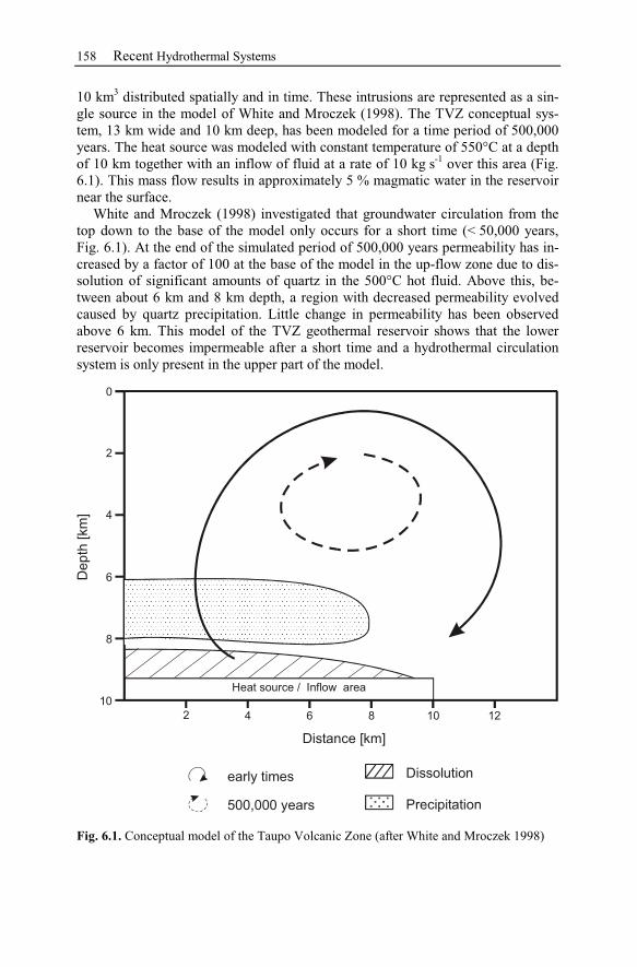
158 Recent Hydrothermal Systems
10 km3 distributed spatially and in time. These intrusions are represented as a sin-
gle source in the model of White and Mroczek (1998). The TVZ conceptual sys-
tem, 13 km wide and 10 km deep, has been modeled for a time period of 500,000
years. The heat source was modeled with constant temperature of 550°C at a depth
of 10 km together with an inflow of fluid at a rate of 10 kg s-1
over this area (Fig.
6.1). This mass flow results in approximately 5 % magmatic water in the reservoir
near the surface.
White and Mroczek (1998) investigated that groundwater circulation from the
top down to the base of the model only occurs for a short time (< 50,000 years,
Fig. 6.1). At the end of the simulated period of 500,000 years permeability has in-
creased by a factor of 100 at the base of the model in the up-flow zone due to dis-
solution of significant amounts of quartz in the 500°C hot fluid. Above this, be-
tween about 6 km and 8 km depth, a region with decreased permeability evolved
caused by quartz precipitation. Little change in permeability has been observed
above 6 km. This model of the TVZ geothermal reservoir shows that the lower
reservoir becomes impermeable after a short time and a hydrothermal circulation
system is only present in the upper part of the model.
2 4 6 8 10 12
10
8
6
4
2
0
Heat source / Inflow area
Distance [km]
De
pth
[km
]
early times
500,000 years Precipitation
Dissolution
Fig. 6.1. Conceptual model of the Taupo Volcanic Zone (after White and Mroczek 1998)
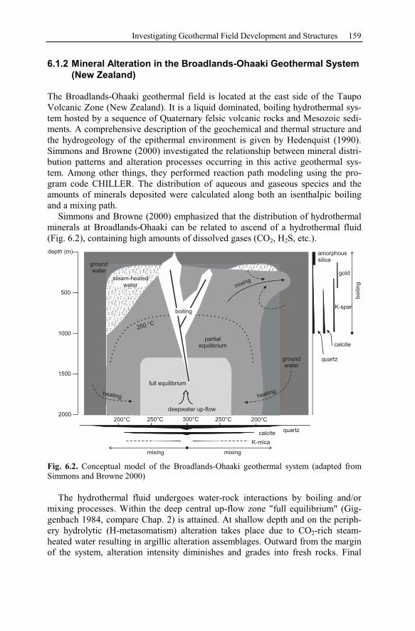
Investigating Geothermal Field Development and Structures 159
6.1.2 Mineral Alteration in the Broadlands-Ohaaki Geothermal System
(New Zealand)
The Broadlands-Ohaaki geothermal field is located at the east side of the Taupo
Volcanic Zone (New Zealand). It is a liquid dominated, boiling hydrothermal sys-
tem hosted by a sequence of Quaternary felsic volcanic rocks and Mesozoic sedi-
ments. A comprehensive description of the geochemical and thermal structure and
the hydrogeology of the epithermal environment is given by Hedenquist (1990).
Simmons and Browne (2000) investigated the relationship between mineral distri-
bution patterns and alteration processes occurring in this active geothermal sys-
tem. Among other things, they performed reaction path modeling using the pro-
gram code CHILLER. The distribution of aqueous and gaseous species and the
amounts of minerals deposited were calculated along both an isenthalpic boiling
and a mixing path.
Simmons and Browne (2000) emphasized that the distribution of hydrothermal
minerals at Broadlands-Ohaaki can be related to ascend of a hydrothermal fluid
(Fig. 6.2), containing high amounts of dissolved gases (CO2, H2S, etc.).
deepwater up-flow
heatingheating
ground
water
ground
water
full equilibrium
partial
equilibrium
250 °C
boiling
steam-heated
water mixing
2000
1500
1000
500
depth (m)
200°C 200°C300°C 250°C250°C
amorphous
silica
quartz
calcite
K-spar
gold
bo
ilin
g
quartzcalcite
K-mica
mixingmixing
Fig. 6.2. Conceptual model of the Broadlands-Ohaaki geothermal system (adapted from
Simmons and Browne 2000)
The hydrothermal fluid undergoes water-rock interactions by boiling and/or
mixing processes. Within the deep central up-flow zone "full equilibrium" (Gig-
genbach 1984, compare Chap. 2) is attained. At shallow depth and on the periph-
ery hydrolytic (H-metasomatism) alteration takes place due to CO2-rich steam-
heated water resulting in argillic alteration assemblages. Outward from the margin
of the system, alteration intensity diminishes and grades into fresh rocks. Final
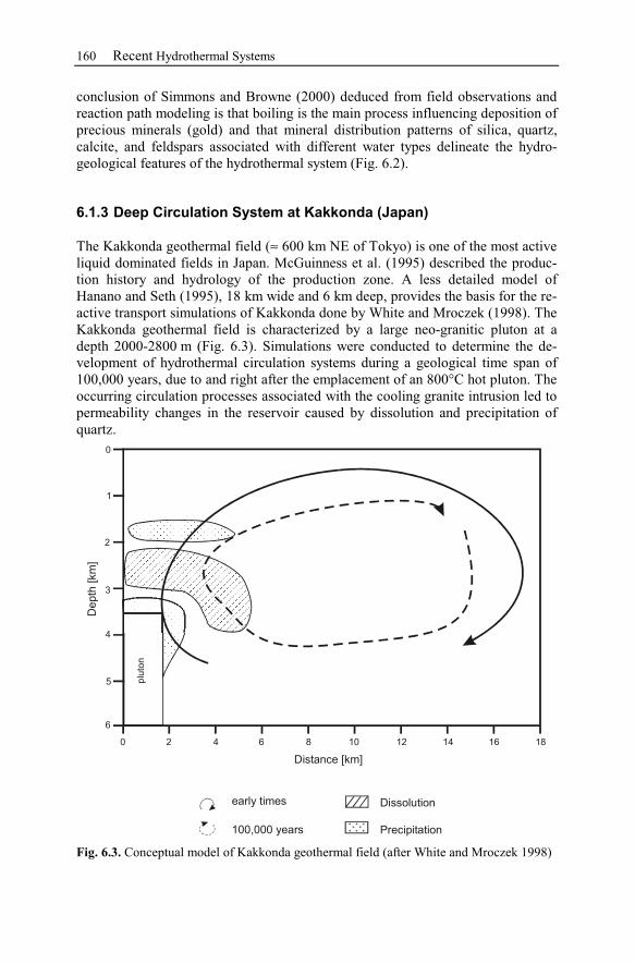
160 Recent Hydrothermal Systems
conclusion of Simmons and Browne (2000) deduced from field observations and
reaction path modeling is that boiling is the main process influencing deposition of
precious minerals (gold) and that mineral distribution patterns of silica, quartz,
calcite, and feldspars associated with different water types delineate the hydro-
geological features of the hydrothermal system (Fig. 6.2).
6.1.3 Deep Circulation System at Kakkonda (Japan)
The Kakkonda geothermal field (≈ 600 km NE of Tokyo) is one of the most active
liquid dominated fields in Japan. McGuinness et al. (1995) described the produc-
tion history and hydrology of the production zone. A less detailed model of
Hanano and Seth (1995), 18 km wide and 6 km deep, provides the basis for the re-
active transport simulations of Kakkonda done by White and Mroczek (1998). The
Kakkonda geothermal field is characterized by a large neo-granitic pluton at a
depth 2000-2800 m (Fig. 6.3). Simulations were conducted to determine the de-
velopment of hydrothermal circulation systems during a geological time span of
100,000 years, due to and right after the emplacement of an 800°C hot pluton. The
occurring circulation processes associated with the cooling granite intrusion led to
permeability changes in the reservoir caused by dissolution and precipitation of
quartz.
Distance [km]
early times
100,000 years Precipitation
Dissolution
0 2 4 6 8 10 12 14 16 18
6
5
4
3
2
1
0
Depth
[km
]
plu
ton
Fig. 6.3. Conceptual model of Kakkonda geothermal field (after White and Mroczek 1998)
Investigating Geothermal Field Development and Structures 161
White and Mroczek (1998) observed permeability reduction above the granitic
intrusion as a result of hydrothermal convection and reactive transport during
early times (Fig. 6.3). Permeability reduction occurred during the whole modeled
time period caused by the reduced silica solubility near the critical point of water.
Above the region with reduced permeability follows a region of enhanced perme-
ability and a second area of reduced permeability (Fig. 6.3). Enhancement of per-
meability is due to cool water being drawn into the up-flow zone and becoming
undersaturated in silica when heated. Ascending within the up-flow zone the water
cools and becomes finally supersaturated in silica and precipitation begins. The fi-
nal convection cell after 100,000 years results from silica precipitation and ac-
companying permeability reduction.
6.1.4 Alteration Halo of a Diorite Intrusion
White and Christenson (2000, 2002) investigated the alteration halo of an ideal-
ized diorite intrusion, because magmatic intrusions are often the heat sources of
geothermal fields (for example Kakkonda, Sasada et al. 1998). The idealized
simulations of an intrusion, here according to the diorite body intersected during
drilling in the Ngatamariki field (New Zealand, Christenson et al. 1997), were per-
formed with CHEM-TOUGH. Extensive hydrothermal alteration within the plu-
tonic rock and in a halo surrounding it suggests that it acted as a heat source for a
convective hydrothermal system. The simulations focused on the influence of
magmatic vapor intruding into the base of a geothermal reservoir and resulting al-
teration around the magmatic intrusion as well as water compositions in shallow
parts of the field, due to fluid flow, heat transfer, transport, and reaction processes.
The model of White and Christenson (2002) takes into consideration thermal
and chemical effects right after emplacement of the diorite intrusion. The hydro-
thermal reservoir contains a reactive fluid dominated by CO2. White and Christen-
son (2000) demonstrated the possibility to simulate the effect of a pulse of mag-
matic vapour (CO2, SO2, H2S, HCl) into the base of a reservoir and to calculate
changing chemical and physical conditions over a time period of 15,000 years.
They observed convective upwelling above the intrusion (comparable to TVZ,
Fig. 6.1) with highly oxidizing fluids near the heat and vapor source. The addition
of the volatiles resulted in hydrolysis reactions and led to dissolution of albite and
anorthite close to the intrusion. Elemental sulfur and alunite form in the low pH
and oxidizing environment. Similarly, Ca2+
released from anorthite is taken up in
anhydrite.
The reactive transport approach of White and Christenson (2002) shows a way
to set up concepts for reactions occurring in the environment of unexplored heat
sources at depth and to associate with it fluid chemistry and alteration products
observed in shallow parts of the reservoirs.
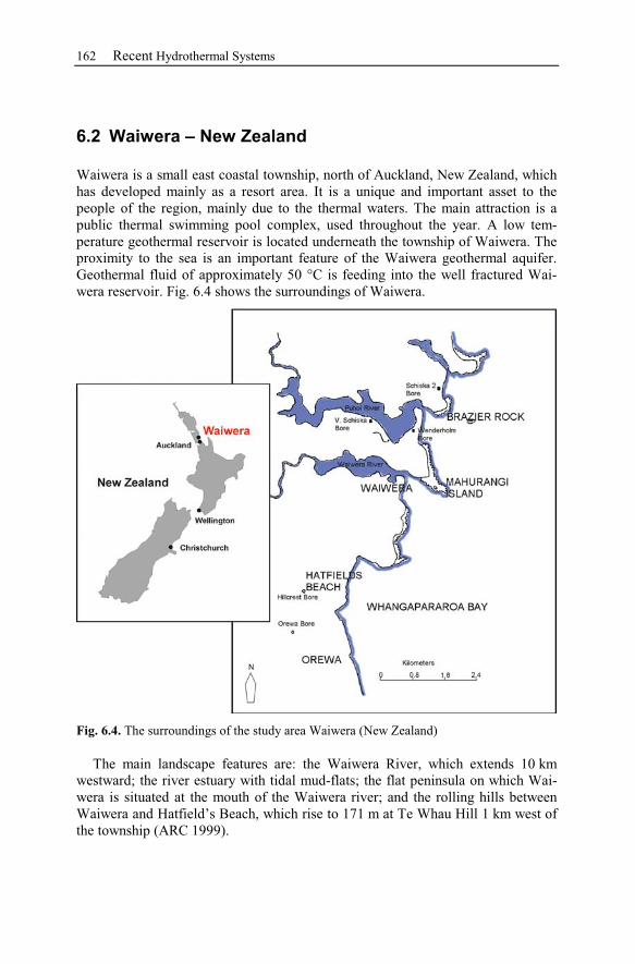
162 Recent Hydrothermal Systems
6.2 Waiwera – New Zealand
Waiwera is a small east coastal township, north of Auckland, New Zealand, which
has developed mainly as a resort area. It is a unique and important asset to the
people of the region, mainly due to the thermal waters. The main attraction is a
public thermal swimming pool complex, used throughout the year. A low tem-
perature geothermal reservoir is located underneath the township of Waiwera. The
proximity to the sea is an important feature of the Waiwera geothermal aquifer.
Geothermal fluid of approximately 50 °C is feeding into the well fractured Wai-
wera reservoir. Fig. 6.4 shows the surroundings of Waiwera.
Fig. 6.4. The surroundings of the study area Waiwera (New Zealand)
The main landscape features are: the Waiwera River, which extends 10 km
westward; the river estuary with tidal mud-flats; the flat peninsula on which Wai-
wera is situated at the mouth of the Waiwera river; and the rolling hills between
Waiwera and Hatfield’s Beach, which rise to 171 m at Te Whau Hill 1 km west of
the township (ARC 1999).
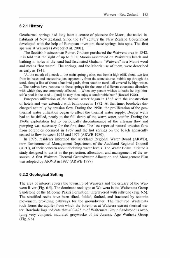
Waiwera – New Zealand 163
6.2.1 History
Geothermal springs had long been a source of pleasure for Maori, the native in-
habitants of New Zealand. Since the 19th
century the New Zealand Government
developed with the help of European investors these springs into spas. The first
spa was at Waiwera (Weeber et al. 2001).
The Scottish businessman Robert Graham purchased the Waiwera area in 1842.
It is told that the sight of up to 3000 Maoris assembled on Waiwera's beach and
bathing in holes in the sand had fascinated Graham. "Waiwera" is a Maori word
and means "hot water". The springs, and the Maoris use of them, were described
as early as 1841:
"At the mouth of a creek ... the main spring gushes out from a high cliff, about two feet
from its base; and successive jets, apparently from the same source, bubble up through the
sand, along a line of about a hundred yards, from south to north, all covered by high water.
... The natives have recourse to these springs for the cure of different cutaneous disorders
with which they are commonly affected. ... When any person wishes to bathe he digs him-
self a pool in the sand ... [and] he may then enjoy a comfortable bath" (Rockel 1986).
European utilization of the thermal water began in 1863 with the construction
of hotels and was extended with bathhouses in 1872. At that time, boreholes dis-
charged naturally by artesian flow. During the 1950s, the proliferation of the geo-
thermal water utilization began to affect the thermal water supply. Deeper wells
had to be drilled, nearly to the full depth of the warm water aquifer. During the
1960s exploitation led to periodically discontinuance of the artesian flow and
pumping was necessary for the first time. The last reported natural artesian flow
from boreholes occurred in 1969 and the hot springs on the beach apparently
ceased to flow between 1975 and 1976 (ARWB 1980).
In 1975, residents informed the Auckland Regional Water Board (ARWB),
now Environmental Management Department of the Auckland Regional Council
(ARC), of their concern about declining water levels. The Water Board initiated a
study designed to assist in the protection, allocation, and management of the re-
source. A first Waiwera Thermal Groundwater Allocation and Management Plan
was adopted by ARWB in 1987 (ARWB 1987)
6.2.2 Geological Setting
The area of interest covers the township of Waiwera and the estuary of the Wai-
wera River (Fig. 6.5). The dominant rock type at Waiwera is the Waitemata Group
Sandstone of the Miocene Pakiri Formation, interlayered with siltstone (Fig. 6.6).
The stratified rocks have been tilted, folded, faulted, and fractured by tectonic
movement, providing pathways for the groundwater. The fractured Waitemata
rock forms the aquifer from which the boreholes at Waiwera extract thermal wa-
ter. Borehole logs indicate that 400-425 m of Waitemata Group Sandstone is over-
lying very compact, indurated greywacke of the Jurassic Age Waiheke Group
(Fig. 6.6).
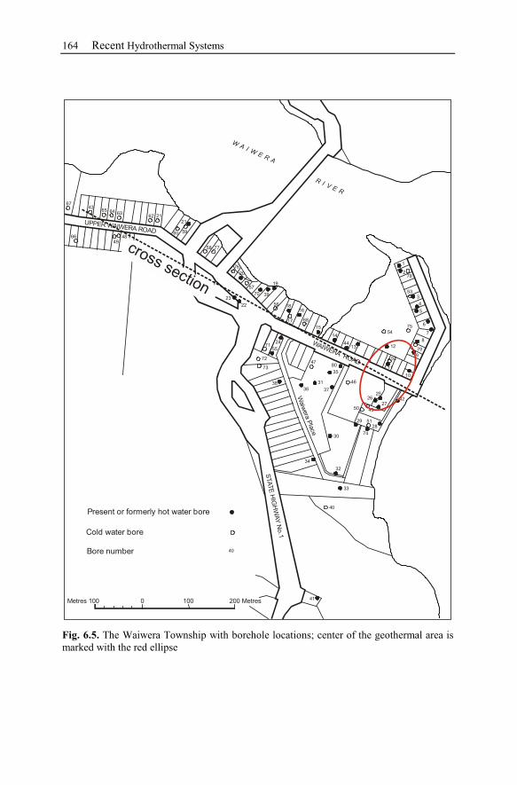
164 Recent Hydrothermal Systems
Metres 100 200 Metres1000
Present or formerly hot water bore
Cold water bore
Bore number 40
41
33
32
34
74
28
5129
50
37
35
46
80
36
38
73
72
55
24
14
44
11
10
9
8
7
6
5
4
3
1
15
17
18
16
68
5622
23
1957
20
76
39
7758
5960
21
2162
6443
65
67
66
49
48
70
2
53
13
54
75
7912
52
71
31
47
2625
45
42
27
40
30
WAI W
ERA
RI V
ER
UPPER WAIWERA ROAD
WAIWERAROAD
Waiw
era
Pla
ce
STA
TE
HIG
HW
AY
No.1
78
crosssection
Fig. 6.5. The Waiwera Township with borehole locations; center of the geothermal area is
marked with the red ellipse
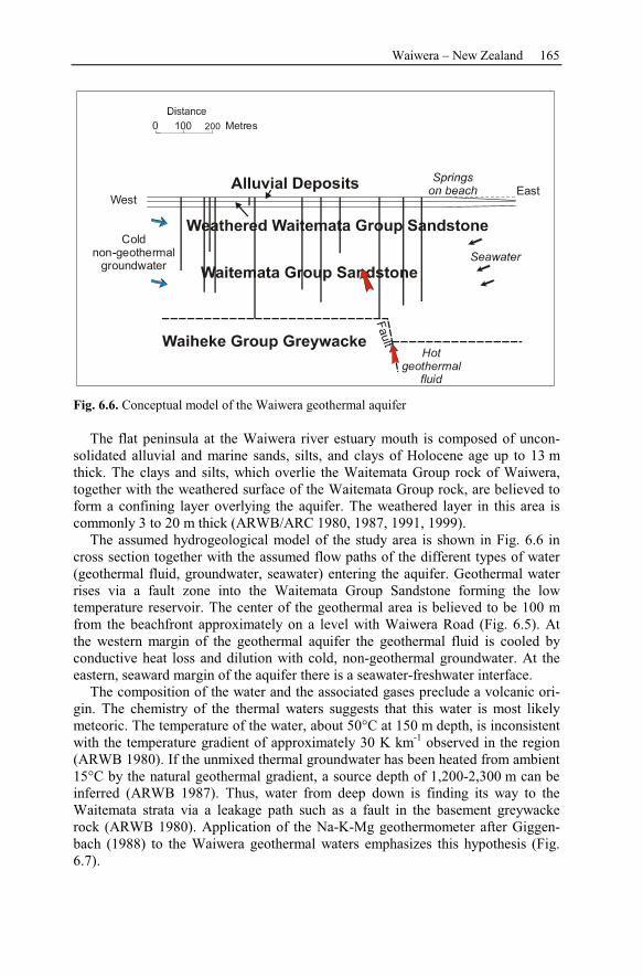
Waiwera – New Zealand 165
West
Cold
non-geothermal
groundwater
Hot
geothermal
fluid
East
0 200 Metres
Fig. 6.6. Conceptual model of the Waiwera geothermal aquifer
The flat peninsula at the Waiwera river estuary mouth is composed of uncon-
solidated alluvial and marine sands, silts, and clays of Holocene age up to 13 m
thick. The clays and silts, which overlie the Waitemata Group rock of Waiwera,
together with the weathered surface of the Waitemata Group rock, are believed to
form a confining layer overlying the aquifer. The weathered layer in this area is
commonly 3 to 20 m thick (ARWB/ARC 1980, 1987, 1991, 1999).
The assumed hydrogeological model of the study area is shown in Fig. 6.6 in
cross section together with the assumed flow paths of the different types of water
(geothermal fluid, groundwater, seawater) entering the aquifer. Geothermal water
rises via a fault zone into the Waitemata Group Sandstone forming the low
temperature reservoir. The center of the geothermal area is believed to be 100 m
from the beachfront approximately on a level with Waiwera Road (Fig. 6.5). At
the western margin of the geothermal aquifer the geothermal fluid is cooled by
conductive heat loss and dilution with cold, non-geothermal groundwater. At the
eastern, seaward margin of the aquifer there is a seawater-freshwater interface.
The composition of the water and the associated gases preclude a volcanic ori-
gin. The chemistry of the thermal waters suggests that this water is most likely
meteoric. The temperature of the water, about 50°C at 150 m depth, is inconsistent
with the temperature gradient of approximately 30 K km-1
observed in the region
(ARWB 1980). If the unmixed thermal groundwater has been heated from ambient
15°C by the natural geothermal gradient, a source depth of 1,200-2,300 m can be
inferred (ARWB 1987). Thus, water from deep down is finding its way to the
Waitemata strata via a leakage path such as a fault in the basement greywacke
rock (ARWB 1980). Application of the Na-K-Mg geothermometer after Giggen-
bach (1988) to the Waiwera geothermal waters emphasizes this hypothesis (Fig.
6.7).
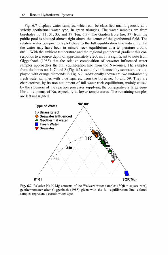
166 Recent Hydrothermal Systems
Fig. 6.7 displays water samples, which can be classified unambiguously as a
strictly geothermal water type, in green triangles. The water samples are from
boreholes no. 11, 31, 35, and 37 (Fig. 6.5). The Garden Bore (no. 37) from the
public pool is situated almost right above the center of the geothermal field. The
relative water compositions plot close to the full equilibration line indicating that
the water may have been in mineral-rock equilibrium at a temperature around
80°C. With the ambient temperature and the regional geothermal gradient this cor-
responds to a source depth of approximately 2,200 m. It is significant to note from
Giggenbach (1988) that the relative composition of seawater influenced water
samples approaches the full equilibration line from the Na-corner. The samples
from the bores no. 1, 7, and 8 (Fig. 6.5), certainly influenced by seawater, are dis-
played with orange diamonds in Fig. 6.7. Additionally shown are two undoubtedly
fresh water samples with blue squares, from the bores no. 40 and 59. They are
characterized by its non-attainment of full water rock equilibrium, mainly caused
by the slowness of the reaction processes supplying the comparatively large equi-
librium contents of Na, especially at lower temperatures. The remaining samples
are left unassigned.
K*.01 SQR(Mg)
Na*.001
80
160
240
320
Type of Water
Unassigned
Seawater influenced
Geothermal water
Fresh Water
Seawater
Fig. 6.7. Relative Na-K-Mg contents of the Waiwera water samples (SQR = square root);
geothermometer after Giggenbach (1988) given with the full equilibration line; colored
samples represent a certain water type
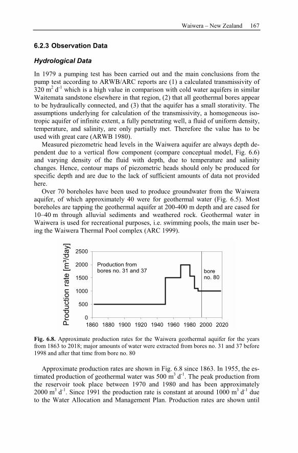
Waiwera – New Zealand 167
6.2.3 Observation Data
Hydrological Data
In 1979 a pumping test has been carried out and the main conclusions from the
pump test according to ARWB/ARC reports are (1) a calculated transmissivity of
320 m2 d
-1 which is a high value in comparison with cold water aquifers in similar
Waitemata sandstone elsewhere in that region, (2) that all geothermal bores appear
to be hydraulically connected, and (3) that the aquifer has a small storativity. The
assumptions underlying for calculation of the transmissivity, a homogeneous iso-
tropic aquifer of infinite extent, a fully penetrating well, a fluid of uniform density,
temperature, and salinity, are only partially met. Therefore the value has to be
used with great care (ARWB 1980).
Measured piezometric head levels in the Waiwera aquifer are always depth de-
pendent due to a vertical flow component (compare conceptual model, Fig. 6.6)
and varying density of the fluid with depth, due to temperature and salinity
changes. Hence, contour maps of piezometric heads should only be produced for
specific depth and are due to the lack of sufficient amounts of data not provided
here.
Over 70 boreholes have been used to produce groundwater from the Waiwera
aquifer, of which approximately 40 were for geothermal water (Fig. 6.5). Most
boreholes are tapping the geothermal aquifer at 200-400 m depth and are cased for
10–40 m through alluvial sediments and weathered rock. Geothermal water in
Waiwera is used for recreational purposes, i.e. swimming pools, the main user be-
ing the Waiwera Thermal Pool complex (ARC 1999).
1860 1880 1900 1920 1940 1960 1980 2000 2020Pro
du
ctio
n r
ate
[m
³/d
ay]
0
500
1000
1500
2000
2500
Production from
bores no. 31 and 37 bore
no. 80
Fig. 6.8. Approximate production rates for the Waiwera geothermal aquifer for the years
from 1863 to 2018; major amounts of water were extracted from bores no. 31 and 37 before
1998 and after that time from bore no. 80
Approximate production rates are shown in Fig. 6.8 since 1863. In 1955, the es-
timated production of geothermal water was 500 m3 d
-1. The peak production from
the reservoir took place between 1970 and 1980 and has been approximately
2000 m3 d
-1. Since 1991 the production rate is constant at around 1000 m
3 d
-1 due
to the Water Allocation and Management Plan. Production rates are shown until
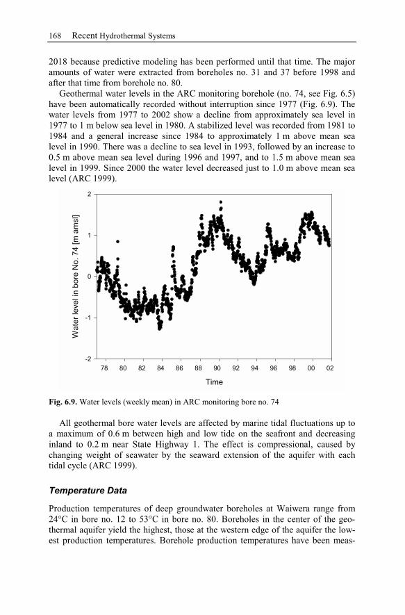
168 Recent Hydrothermal Systems
2018 because predictive modeling has been performed until that time. The major
amounts of water were extracted from boreholes no. 31 and 37 before 1998 and
after that time from borehole no. 80.
Geothermal water levels in the ARC monitoring borehole (no. 74, see Fig. 6.5)
have been automatically recorded without interruption since 1977 (Fig. 6.9). The
water levels from 1977 to 2002 show a decline from approximately sea level in
1977 to 1 m below sea level in 1980. A stabilized level was recorded from 1981 to
1984 and a general increase since 1984 to approximately 1 m above mean sea
level in 1990. There was a decline to sea level in 1993, followed by an increase to
0.5 m above mean sea level during 1996 and 1997, and to 1.5 m above mean sea
level in 1999. Since 2000 the water level decreased just to 1.0 m above mean sea
level (ARC 1999).
Time
78 80 82 84 86 88 90 92 94 96 98 00 02
Wate
r le
ve
l in
bore
No
. 74
[m
am
sl]
-2
-1
0
1
2
Fig. 6.9. Water levels (weekly mean) in ARC monitoring bore no. 74
All geothermal bore water levels are affected by marine tidal fluctuations up to
a maximum of 0.6 m between high and low tide on the seafront and decreasing
inland to 0.2 m near State Highway 1. The effect is compressional, caused by
changing weight of seawater by the seaward extension of the aquifer with each
tidal cycle (ARC 1999).
Temperature Data
Production temperatures of deep groundwater boreholes at Waiwera range from
24°C in bore no. 12 to 53°C in bore no. 80. Boreholes in the center of the geo-
thermal aquifer yield the highest, those at the western edge of the aquifer the low-
est production temperatures. Borehole production temperatures have been meas-
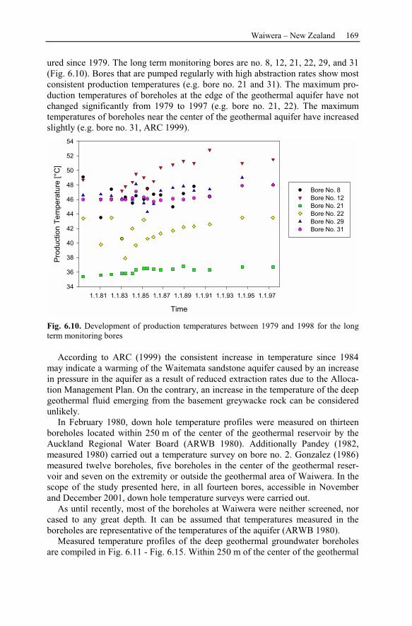
Waiwera – New Zealand 169
ured since 1979. The long term monitoring bores are no. 8, 12, 21, 22, 29, and 31
(Fig. 6.10). Bores that are pumped regularly with high abstraction rates show most
consistent production temperatures (e.g. bore no. 21 and 31). The maximum pro-
duction temperatures of boreholes at the edge of the geothermal aquifer have not
changed significantly from 1979 to 1997 (e.g. bore no. 21, 22). The maximum
temperatures of boreholes near the center of the geothermal aquifer have increased
slightly (e.g. bore no. 31, ARC 1999).
Time
1.1.81 1.1.83 1.1.85 1.1.87 1.1.89 1.1.91 1.1.93 1.1.95 1.1.97
Pro
du
ctio
n T
em
pe
ratu
re [
°C
]
34
36
38
40
42
44
46
48
50
52
54
Bore No. 8
Bore No. 12
Bore No. 21
Bore No. 22
Bore No. 29
Bore No. 31
Fig. 6.10. Development of production temperatures between 1979 and 1998 for the long
term monitoring bores
According to ARC (1999) the consistent increase in temperature since 1984
may indicate a warming of the Waitemata sandstone aquifer caused by an increase
in pressure in the aquifer as a result of reduced extraction rates due to the Alloca-
tion Management Plan. On the contrary, an increase in the temperature of the deep
geothermal fluid emerging from the basement greywacke rock can be considered
unlikely.
In February 1980, down hole temperature profiles were measured on thirteen
boreholes located within 250 m of the center of the geothermal reservoir by the
Auckland Regional Water Board (ARWB 1980). Additionally Pandey (1982,
measured 1980) carried out a temperature survey on bore no. 2. Gonzalez (1986)
measured twelve boreholes, five boreholes in the center of the geothermal reser-
voir and seven on the extremity or outside the geothermal area of Waiwera. In the
scope of the study presented here, in all fourteen bores, accessible in November
and December 2001, down hole temperature surveys were carried out.
As until recently, most of the boreholes at Waiwera were neither screened, nor
cased to any great depth. It can be assumed that temperatures measured in the
boreholes are representative of the temperatures of the aquifer (ARWB 1980).
Measured temperature profiles of the deep geothermal groundwater boreholes
are compiled in Fig. 6.11 - Fig. 6.15. Within 250 m of the center of the geothermal
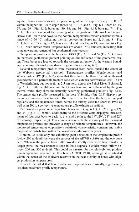
170 Recent Hydrothermal Systems
aquifer, bores show a steady temperature gradient of approximately 0.2 K m-1
within the upper 60–120 m depth (bores no. 2, 3, 7, and 8 - Fig. 6.11; bore no. 19,
27, and 29 - Fig. 6.12; bores no. 30, 34, and 36 - Fig. 6.13; bore no. 74 - Fig.
6.14). This is in excess of the natural geothermal gradient of the Auckland region.
Below 100–140 m and down to the bottom, temperatures remain constant within a
range of 40–50 °C, indicating thermal convection (bores no. 2, 3, and 8 - Fig.
6.11; bore no. 27 - Fig. 6.12; bores no. 34 and 36 - Fig. 6.13; bore no. 74 - Fig.
6.14). Near surface water temperatures are above 15°C ambient, indicating that
some upward movement of hot geothermal water occurs.
Temperature profiles of the bores no. 48/49 (Fig. 6.13) and 66 (Fig. 6.14) show
an increased geothermal gradient pointing out the influence of the geothermal wa-
ter. These bores are located towards the western extremity. At the western bound-
ary the non-geothermal groundwater region is located (Fig. 6.6).
Several temperature profiles were measured from bores outside the center of
the Waiwera geothermal reservoir. Temperature profiles Wenderholme, and
Wenderholme DW (Fig. 6.15) show that there has to be flow of tepid geothermal
groundwater in a permeable fracture zone which extends northward at least 1.5 km
to Wenderholme, but not as far as 2.5 km north across the Puhoi River (Schiska 2,
Fig. 6.14). Both the Hillcrest and the Orewa bore are not influenced by the geo-
thermal water, they show the naturally occurring geothermal gradient (Fig. 6.15).
The temperature profile measured in the bore V Schiska (Fig. 6.14) displays ap-
parently convective heat transfer. But, due to the fact that the bore is pumped
regularly and the unattended times before the survey were too short in 1986 as
well as in 2001, a convective temperature profile exhibits an artifact.
Performed temperature surveys from bores no. 8 (Fig. 6.11), 11, 27 (Fig. 6.12),
and 34 (Fig. 6.13) exhibit, additionally to the different years displayed, measure-
ments of four days back-to-back (a, b, c, and d refer to the 19th
, 20th
, 21st, and 22
nd
of February, respectively). This comparison reflects the accuracy of the measured
temperature profiles and provides a range of reliable temperatures. However, the
monitored temperatures emphasize a relatively characteristic, constant and stable
temperature distribution within the Waiwera aquifer over the years.
Bore no. 36 is the only one exhibiting great deviation in the temperature profile
(below 200 m depth) between the surveys of the ARWB (1980) and the one done
here. Whereas the profile from 1980 provides strictly convective heat transfer in
deeper parts, the measurements done in 2001 suppose a colder water inflow be-
tween 200 and 300 m depth. This could be a reason for the relatively low produc-
tion temperature observed in this bore (ARWB 1980), although it is situated
within the center of the Waiwera reservoir in the near vicinity of bores with high-
est production temperatures.
It has to be noted that bore production temperatures are usually, significantly
less than maximum profile temperature.
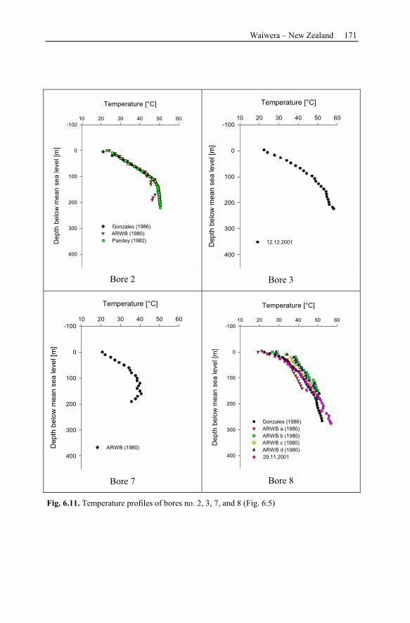
Waiwera – New Zealand 171
Temperature [°C]
10 20 30 40 50 60
De
pth
be
low
me
an
se
a leve
l [m
]
-100
0
100
200
300
400
Gonzales (1986)
ARWB (1980)
Pandey (1982)
Bore 2
Temperature [°C]
10 20 30 40 50 60
Dep
th b
elo
w m
ea
n s
ea le
ve
l [m
]
-100
0
100
200
300
400
12.12.2001
Bore 3
Temperature [°C]
10 20 30 40 50 60
Dep
th b
elo
w m
ea
n s
ea le
ve
l [m
]
-100
0
100
200
300
400
ARWB (1980)
Bore 7
Temperature [°C]
10 20 30 40 50 60
De
pth
be
low
me
an
se
a leve
l [m
]
-100
0
100
200
300
400
Gonzales (1986)
ARWB a (1980)
ARWB b (1980)
ARWB c (1980)
ARWB d (1980)
29.11.2001
Bore 8
Fig. 6.11. Temperature profiles of bores no. 2, 3, 7, and 8 (Fig. 6.5)
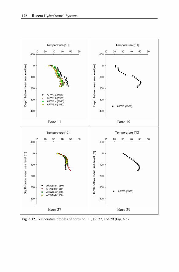
172 Recent Hydrothermal Systems
Temperature [°C]
10 20 30 40 50 60
De
pth
be
low
me
an
se
a leve
l [m
]
-100
0
100
200
300
400
ARWB a (1980)
ARWB b (1980)
ARWB c (1980)
ARWB d (1980)
Bore 11
Temperature [°C]
10 20 30 40 50 60
De
pth
be
low
me
an
se
a leve
l [m
]
-100
0
100
200
300
400
ARWB (1980)
Bore 19
Temperature [°C]
10 20 30 40 50 60
De
pth
be
low
me
an
se
a leve
l [m
]
-100
0
100
200
300
400
ARWB a (1980)
ARWB b (1980)
ARWB c (1980)
ARWB d (1980)
Bore 27
Temperature [°C]
10 20 30 40 50 60
Dep
th b
elo
w m
ean
sea leve
l [m
]
-100
0
100
200
300
400
ARWB (1980)
Bore 29
Fig. 6.12. Temperature profiles of bores no. 11, 19, 27, and 29 (Fig. 6.5)
Waiwera – New Zealand 173
Temperature [°C]
10 20 30 40 50 60
Dep
th b
elo
w m
ean
sea leve
l [m
]
-100
0
100
200
300
400
Gonzales (1986)
ARWB (1980)
Bore 30
Temperature [°C]
10 20 30 40 50 60
De
pth
be
low
me
an
se
a leve
l [m
]
-100
0
100
200
300
400
Gonzales a (1986)
Gonzales b (1986)
ARWB a (1980)
ARWB b (1980)
ARWB c (1980)
30.11.2001
Bore 34
Temperature [°C]
10 20 30 40 50 60
Dep
th b
elo
w m
ean
sea leve
l [m
]
-100
0
100
200
300
400
ARWB (1980)
29.11.2001 (down)
29.11.2001 (up)
12.12.2001
Bore 36
Temperature [°C]
10 20 30 40 50 60
De
pth
be
low
me
an
se
a leve
l [m
]
-100
0
100
200
300
400
Gonzales # 48 (1986)
Gonzales #49 (1986)
12.12.2001
Bore 48/49
Fig. 6.13. Temperature profiles of bores no. 30, 34, 36, and 48/49 (Fig. 6.5)
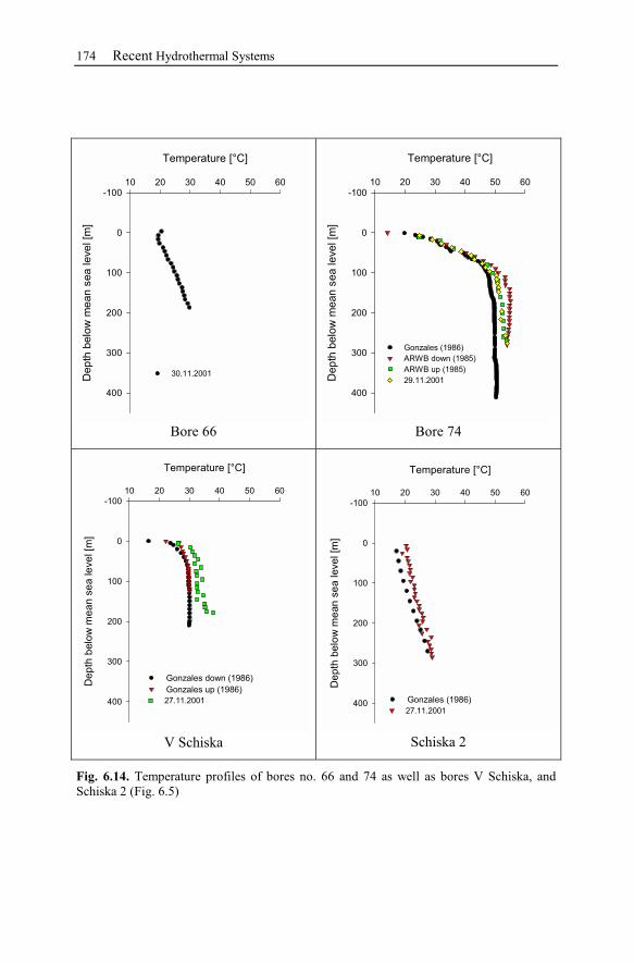
174 Recent Hydrothermal Systems
Temperature [°C]
10 20 30 40 50 60
Dep
th b
elo
w m
ean
sea leve
l [m
]
-100
0
100
200
300
400
30.11.2001
Bore 66
Temperature [°C]
10 20 30 40 50 60
Dep
th b
elo
w m
ean
sea leve
l [m
]
-100
0
100
200
300
400
Gonzales (1986)
ARWB down (1985)
ARWB up (1985)
29.11.2001
Bore 74
Temperature [°C]
10 20 30 40 50 60
De
pth
belo
w m
ea
n s
ea
le
ve
l [m
]
-100
0
100
200
300
400
Gonzales down (1986)
Gonzales up (1986)
27.11.2001
V Schiska
Temperature [°C]
10 20 30 40 50 60
De
pth
be
low
me
an
se
a leve
l [m
]
-100
0
100
200
300
400Gonzales (1986)
27.11.2001
Schiska 2
Fig. 6.14. Temperature profiles of bores no. 66 and 74 as well as bores V Schiska, and
Schiska 2 (Fig. 6.5)
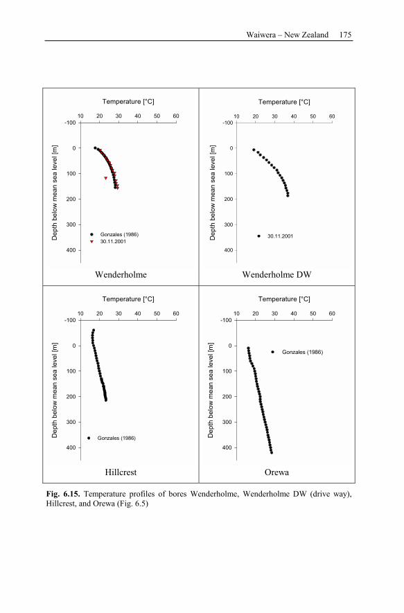
Waiwera – New Zealand 175
Temperature [°C]
10 20 30 40 50 60
De
pth
be
low
me
an
se
a leve
l [m
]
-100
0
100
200
300
400
Gonzales (1986)
30.11.2001
Wenderholme
Temperature [°C]
10 20 30 40 50 60
De
pth
be
low
me
an
se
a leve
l [m
]
-100
0
100
200
300
400
30.11.2001
Wenderholme DW
Temperature [°C]
10 20 30 40 50 60
De
pth
be
low
me
an
se
a leve
l [m
]
-100
0
100
200
300
400
Gonzales (1986)
Hillcrest
Temperature [°C]
10 20 30 40 50 60
De
pth
be
low
me
an
se
a leve
l [m
]
-100
0
100
200
300
400
Gonzales (1986)
Orewa
Fig. 6.15. Temperature profiles of bores Wenderholme, Wenderholme DW (drive way),
Hillcrest, and Orewa (Fig. 6.5)
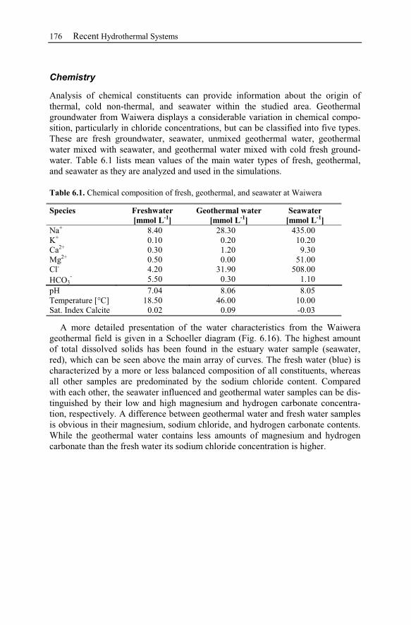
176 Recent Hydrothermal Systems
Chemistry
Analysis of chemical constituents can provide information about the origin of
thermal, cold non-thermal, and seawater within the studied area. Geothermal
groundwater from Waiwera displays a considerable variation in chemical compo-
sition, particularly in chloride concentrations, but can be classified into five types.
These are fresh groundwater, seawater, unmixed geothermal water, geothermal
water mixed with seawater, and geothermal water mixed with cold fresh ground-
water. Table 6.1 lists mean values of the main water types of fresh, geothermal,
and seawater as they are analyzed and used in the simulations.
Table 6.1. Chemical composition of fresh, geothermal, and seawater at Waiwera
Species Freshwater
[mmol L-1
]
Geothermal water
[mmol L-1
]
Seawater
[mmol L-1
]
Na+ 8.40 28.30 435.00
K+ 0.10 0.20 10.20
Ca2+
0.30 1.20 9.30
Mg2+
0.50 0.00 51.00
Cl- 4.20 31.90 508.00
HCO3
-5.50 0.30 1.10
pH 7.04 8.06 8.05
Temperature [°C] 18.50 46.00 10.00
Sat. Index Calcite 0.02 0.09 -0.03
A more detailed presentation of the water characteristics from the Waiwera
geothermal field is given in a Schoeller diagram (Fig. 6.16). The highest amount
of total dissolved solids has been found in the estuary water sample (seawater,
red), which can be seen above the main array of curves. The fresh water (blue) is
characterized by a more or less balanced composition of all constituents, whereas
all other samples are predominated by the sodium chloride content. Compared
with each other, the seawater influenced and geothermal water samples can be dis-
tinguished by their low and high magnesium and hydrogen carbonate concentra-
tion, respectively. A difference between geothermal water and fresh water samples
is obvious in their magnesium, sodium chloride, and hydrogen carbonate contents.
While the geothermal water contains less amounts of magnesium and hydrogen
carbonate than the fresh water its sodium chloride concentration is higher.
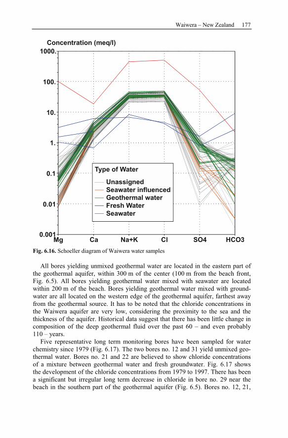
Waiwera – New Zealand 177
Mg Ca Na+K Cl SO4 HCO30.001
0.01
0.1
1.
10.
100.
1000.
Concentration (meq/l)
Type of Water
Unassigned
Seawater influenced
Geothermal water
Fresh Water
Seawater
Fig. 6.16. Schoeller diagram of Waiwera water samples
All bores yielding unmixed geothermal water are located in the eastern part of
the geothermal aquifer, within 300 m of the center (100 m from the beach front,
Fig. 6.5). All bores yielding geothermal water mixed with seawater are located
within 200 m of the beach. Bores yielding geothermal water mixed with ground-
water are all located on the western edge of the geothermal aquifer, farthest away
from the geothermal source. It has to be noted that the chloride concentrations in
the Waiwera aquifer are very low, considering the proximity to the sea and the
thickness of the aquifer. Historical data suggest that there has been little change in
composition of the deep geothermal fluid over the past 60 – and even probably
110 – years.
Five representative long term monitoring bores have been sampled for water
chemistry since 1979 (Fig. 6.17). The two bores no. 12 and 31 yield unmixed geo-
thermal water. Bores no. 21 and 22 are believed to show chloride concentrations
of a mixture between geothermal water and fresh groundwater. Fig. 6.17 shows
the development of the chloride concentrations from 1979 to 1997. There has been
a significant but irregular long term decrease in chloride in bore no. 29 near the
beach in the southern part of the geothermal aquifer (Fig. 6.5). Bores no. 12, 21,

178 Recent Hydrothermal Systems
22, and 31 show no long term consistent change. The chloride concentration in
bore no. 8 increased from 1979 to 1990 followed by a decrease to the initial value
in 1992. No long-term trend in chloride concentrations can be detected for bores at
the western edge of the geothermal aquifer (ARC 1999).
Time
1.1.80 1.1.85 1.1.90 1.1.95
Chlo
ride C
oncen
tra
tion
[g/m
³]
600
800
1000
1200
1400
1600
1800
Bore No. 8
Bore No. 12
Bore No. 21
Bore No. 22
Bore No. 29
Bore No. 31
Fig. 6.17. Long term development of chloride concentrations in monitoring bores
6.2.4 Numerical Simulations
In previous manuscripts the set up of a 3D coupled fluid flow, heat transfer, and
solute transport model of the Waiwera area is described in detail (Stöfen 2000,
Stöfen et al. 2000, Stöfen and Kühn 2003), which is used here to carry out several
numerical investigations using the code SHEMAT. This model defines a natural
state of the Waiwera reservoir and is used to simulate varying scenarios to answer
following questions:
1. Is the conceptual model (Fig. 6.6) of the Waiwera area reasonable?
2. Does seawater intrusion into the aquifer occur?
3. Is the present heat exploitation sustainable?
4. Do chemical reactions alter the reservoir?
Conceptual Model and Boundary Conditions
The following section briefly describes the set up of the numerical model (for de-
tails the reader is referred to Stöfen 2000, Stöfen et al. 2000, Stöfen and Kühn
2003) drawn from the previously discussed concept of the geothermal field of
Waiwera (Fig. 6.6) and the observation data. An equivalent porous medium is as-
sumed to represent the Waiwera aquifer. The applied boundary conditions and
reservoir properties are shown in cross section in Fig. 6.18. Since temperature pro-
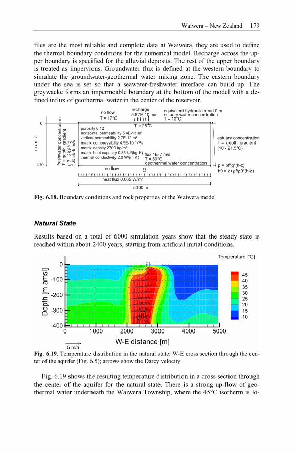
Waiwera – New Zealand 179
files are the most reliable and complete data at Waiwera, they are used to define
the thermal boundary conditions for the numerical model. Recharge across the up-
per boundary is specified for the alluvial deposits. The rest of the upper boundary
is treated as impervious. Groundwater flux is defined at the western boundary to
simulate the groundwater-geothermal water mixing zone. The eastern boundary
under the sea is set so that a seawater-freshwater interface can build up. The
greywacke forms an impermeable boundary at the bottom of the model with a de-
fined influx of geothermal water in the center of the reservoir.
p = ρf*g*(h-z)
h0 = z+ρf/ρ0*(h-z)
no flow
fre
sh
wa
ter
co
ncen
t ra
tio
n
estuary concentration
no flow
geothermal water concentration
heat flux 0.065 W/m²
T = 25°C
T = 17°C
recharge
5.87E-10 m/sequivalent hydraulic head 0 m
estuary water concentration
T = 10°C
T = geoth. gradient
(10 - 21.5°C)
T=
ge
ot h
.g
rad
ien
t
( 17
-2
8. 5
°C
)
flux 1E-7 m/s
T = 50°C
flu
x5
E-9
m/s
0
-410
5000 m
porosity 0.12
horizontal permeability 5.4E-13 m²
vertical permeability 2.7E-12 m²
matrix compressibilty 4.5E-10 1/Pa
matrix density 2700 kg/m³
matrix heat capacity 0.85 kJ/(kg K)
thermal conductivity 2.0 W/(m K)
ma
msl
Fig. 6.18. Boundary conditions and rock properties of the Waiwera model
Natural State
Results based on a total of 6000 simulation years show that the steady state is
reached within about 2400 years, starting from artificial initial conditions.
W-E distance [m]
Dep
th[m
am
sl]
0 1000 2000 3000 4000 5000
-400
-300
-200
-100
0
45
40
35
30
25
20
15
10
Temperature [°C]
5 m/a
Fig. 6.19. Temperature distribution in the natural state; W-E cross section through the cen-
ter of the aquifer (Fig. 6.5); arrows show the Darcy velocity
Fig. 6.19 shows the resulting temperature distribution in a cross section through
the center of the aquifer for the natural state. There is a strong up-flow of geo-
thermal water underneath the Waiwera Township, where the 45°C isotherm is lo-
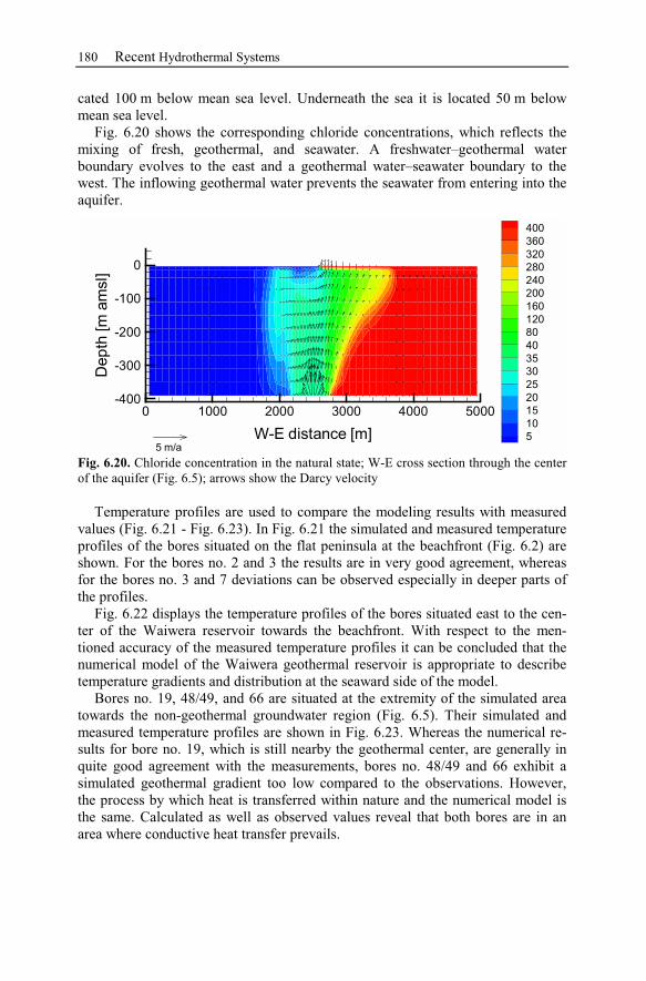
180 Recent Hydrothermal Systems
cated 100 m below mean sea level. Underneath the sea it is located 50 m below
mean sea level.
Fig. 6.20 shows the corresponding chloride concentrations, which reflects the
mixing of fresh, geothermal, and seawater. A freshwater–geothermal water
boundary evolves to the east and a geothermal water–seawater boundary to the
west. The inflowing geothermal water prevents the seawater from entering into the
aquifer.
W-E distance [m]
Dep
th[m
am
sl]
0 1000 2000 3000 4000 5000
-400
-300
-200
-100
0
400
360
320
280
240
200
160
120
80
40
35
30
25
20
15
10
5
5 m/a
Fig. 6.20. Chloride concentration in the natural state; W-E cross section through the center
of the aquifer (Fig. 6.5); arrows show the Darcy velocity
Temperature profiles are used to compare the modeling results with measured
values (Fig. 6.21 - Fig. 6.23). In Fig. 6.21 the simulated and measured temperature
profiles of the bores situated on the flat peninsula at the beachfront (Fig. 6.2) are
shown. For the bores no. 2 and 3 the results are in very good agreement, whereas
for the bores no. 3 and 7 deviations can be observed especially in deeper parts of
the profiles.
Fig. 6.22 displays the temperature profiles of the bores situated east to the cen-
ter of the Waiwera reservoir towards the beachfront. With respect to the men-
tioned accuracy of the measured temperature profiles it can be concluded that the
numerical model of the Waiwera geothermal reservoir is appropriate to describe
temperature gradients and distribution at the seaward side of the model.
Bores no. 19, 48/49, and 66 are situated at the extremity of the simulated area
towards the non-geothermal groundwater region (Fig. 6.5). Their simulated and
measured temperature profiles are shown in Fig. 6.23. Whereas the numerical re-
sults for bore no. 19, which is still nearby the geothermal center, are generally in
quite good agreement with the measurements, bores no. 48/49 and 66 exhibit a
simulated geothermal gradient too low compared to the observations. However,
the process by which heat is transferred within nature and the numerical model is
the same. Calculated as well as observed values reveal that both bores are in an
area where conductive heat transfer prevails.
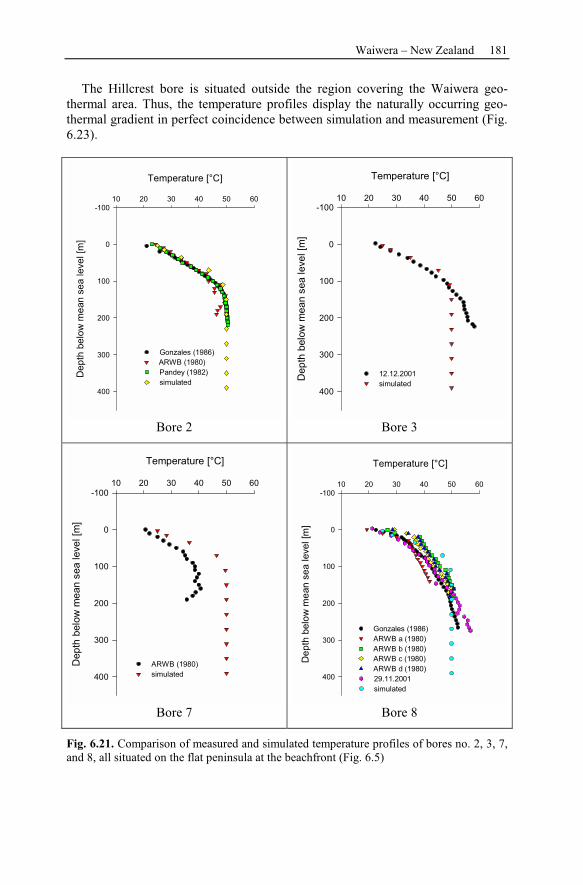
Waiwera – New Zealand 181
The Hillcrest bore is situated outside the region covering the Waiwera geo-
thermal area. Thus, the temperature profiles display the naturally occurring geo-
thermal gradient in perfect coincidence between simulation and measurement (Fig.
6.23).
Temperature [°C]
10 20 30 40 50 60
De
pth
be
low
me
an
se
a leve
l [m
]
-100
0
100
200
300
400
Gonzales (1986)
ARWB (1980)
Pandey (1982)
simulated
Bore 2
Temperature [°C]
10 20 30 40 50 60
Dep
th b
elo
w m
ean
sea leve
l [m
]
-100
0
100
200
300
400
12.12.2001
simulated
Bore 3
Temperature [°C]
10 20 30 40 50 60
Dep
th b
elo
w m
ean
sea leve
l [m
]
-100
0
100
200
300
400
ARWB (1980)
simulated
Bore 7
Temperature [°C]
10 20 30 40 50 60
De
pth
be
low
me
an
se
a leve
l [m
]
-100
0
100
200
300
400
Gonzales (1986)
ARWB a (1980)
ARWB b (1980)
ARWB c (1980)
ARWB d (1980)
29.11.2001
simulated
Bore 8
Fig. 6.21. Comparison of measured and simulated temperature profiles of bores no. 2, 3, 7,
and 8, all situated on the flat peninsula at the beachfront (Fig. 6.5)
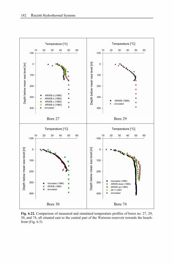
182 Recent Hydrothermal Systems
Temperature [°C]
10 20 30 40 50 60
De
pth
be
low
me
an
se
a leve
l [m
]
-100
0
100
200
300
400
ARWB a (1980)
ARWB b (1980)
ARWB c (1980)
ARWB d (1980)
simulated
Bore 27
Temperature [°C]
10 20 30 40 50 60
Dep
th b
elo
w m
ean
sea leve
l [m
]
-100
0
100
200
300
400
ARWB (1980)
simulated
Bore 29
Temperature [°C]
10 20 30 40 50 60
Dep
th b
elo
w m
ean
sea leve
l [m
]
-100
0
100
200
300
400
Gonzales (1986)
ARWB (1980)
simulated
Bore 30
Temperature [°C]
10 20 30 40 50 60
Dep
th b
elo
w m
ean
sea leve
l [m
]
-100
0
100
200
300
400
Gonzales (1986)
ARWB down (1985)
ARWB up (1985)
29.11.2001
simulated
Bore 74
Fig. 6.22. Comparison of measured and simulated temperature profiles of bores no. 27, 29,
30, and 74, all situated east to the central part of the Waiwera reservoir towards the beach-
front (Fig. 6.5)
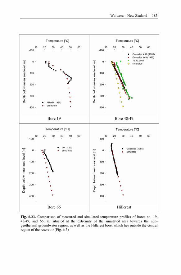
Waiwera – New Zealand 183
Temperature [°C]
10 20 30 40 50 60
De
pth
be
low
me
an
se
a leve
l [m
]
-100
0
100
200
300
400
ARWB (1980)
simulated
Bore 19
Temperature [°C]
10 20 30 40 50 60
De
pth
be
low
me
an
se
a leve
l [m
]
-100
0
100
200
300
400
Gonzales # 48 (1986)
Gonzales #49 (1986)
12.12.2001
simulated
Bore 48/49
Temperature [°C]
10 20 30 40 50 60
Dep
th b
elo
w m
ean
sea leve
l [m
]
-100
0
100
200
300
400
30.11.2001
simulated
Bore 66
Temperature [°C]
10 20 30 40 50 60
De
pth
be
low
me
an
se
a leve
l [m
]
-100
0
100
200
300
400
Gonzales (1986)
simulated
Hillcrest
Fig. 6.23. Comparison of measured and simulated temperature profiles of bores no. 19,
48/49, and 66, all situated at the extremity of the simulated area towards the non-
geothermal groundwater region, as well as the Hillcrest bore, which lies outside the central
region of the reservoir (Fig. 6.5)
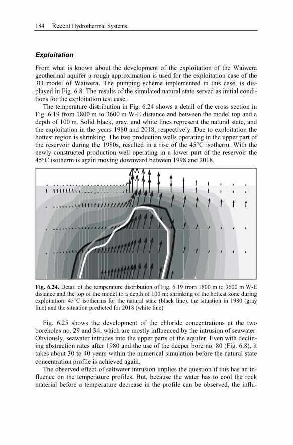
184 Recent Hydrothermal Systems
Exploitation
From what is known about the development of the exploitation of the Waiwera
geothermal aquifer a rough approximation is used for the exploitation case of the
3D model of Waiwera. The pumping scheme implemented in this case, is dis-
played in Fig. 6.8. The results of the simulated natural state served as initial condi-
tions for the exploitation test case.
The temperature distribution in Fig. 6.24 shows a detail of the cross section in
Fig. 6.19 from 1800 m to 3600 m W-E distance and between the model top and a
depth of 100 m. Solid black, gray, and white lines represent the natural state, and
the exploitation in the years 1980 and 2018, respectively. Due to exploitation the
hottest region is shrinking. The two production wells operating in the upper part of
the reservoir during the 1980s, resulted in a rise of the 45°C isotherm. With the
newly constructed production well operating in a lower part of the reservoir the
45°C isotherm is again moving downward between 1998 and 2018.
Fig. 6.24. Detail of the temperature distribution of Fig. 6.19 from 1800 m to 3600 m W-E
distance and the top of the model to a depth of 100 m; shrinking of the hottest zone during
exploitation: 45°C isotherms for the natural state (black line), the situation in 1980 (gray
line) and the situation predicted for 2018 (white line)
Fig. 6.25 shows the development of the chloride concentrations at the two
boreholes no. 29 and 34, which are mostly influenced by the intrusion of seawater.
Obviously, seawater intrudes into the upper parts of the aquifer. Even with declin-
ing abstraction rates after 1980 and the use of the deeper bore no. 80 (Fig. 6.8), it
takes about 30 to 40 years within the numerical simulation before the natural state
concentration profile is achieved again.
The observed effect of saltwater intrusion implies the question if this has an in-
fluence on the temperature profiles. But, because the water has to cool the rock
material before a temperature decrease in the profile can be observed, the influ-
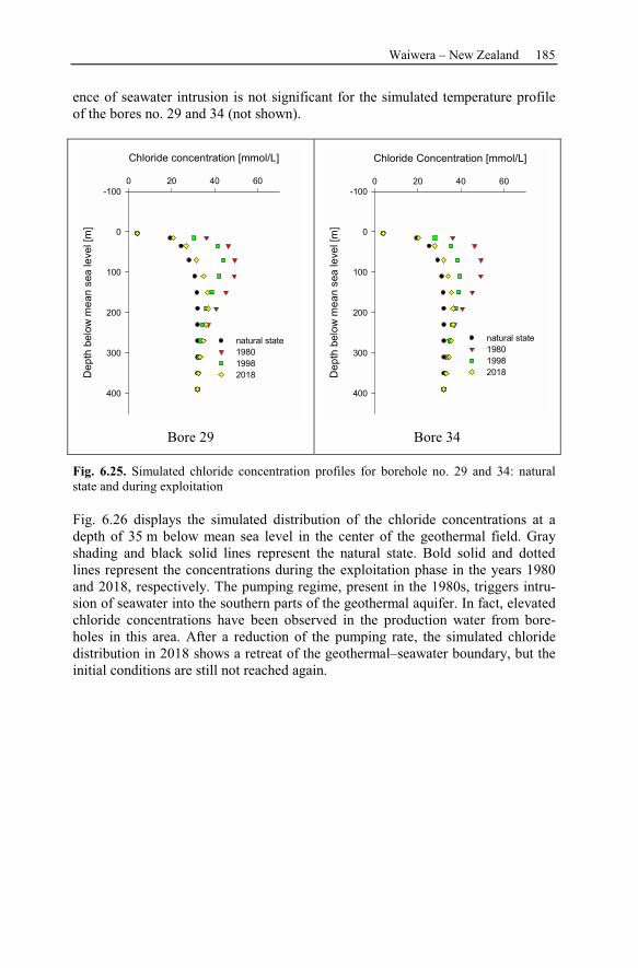
Waiwera – New Zealand 185
ence of seawater intrusion is not significant for the simulated temperature profile
of the bores no. 29 and 34 (not shown).
Chloride concentration [mmol/L]
0 20 40 60
De
pth
be
low
me
an
sea
le
ve
l [m
]
-100
0
100
200
300
400
natural state
1980
1998
2018
Bore 29
Chloride Concentration [mmol/L]
0 20 40 60
De
pth
be
low
me
an
sea
le
ve
l [m
]
-100
0
100
200
300
400
natural state
1980
1998
2018
Bore 34
Fig. 6.25. Simulated chloride concentration profiles for borehole no. 29 and 34: natural
state and during exploitation
Fig. 6.26 displays the simulated distribution of the chloride concentrations at a
depth of 35 m below mean sea level in the center of the geothermal field. Gray
shading and black solid lines represent the natural state. Bold solid and dotted
lines represent the concentrations during the exploitation phase in the years 1980
and 2018, respectively. The pumping regime, present in the 1980s, triggers intru-
sion of seawater into the southern parts of the geothermal aquifer. In fact, elevated
chloride concentrations have been observed in the production water from bore-
holes in this area. After a reduction of the pumping rate, the simulated chloride
distribution in 2018 shows a retreat of the geothermal–seawater boundary, but the
initial conditions are still not reached again.
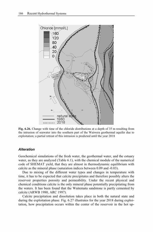
186 Recent Hydrothermal Systems
Fig. 6.26. Change with time of the chloride distributions at a depth of 35 m resulting from
the intrusion of seawater into the southern part of the Waiwera geothermal aquifer due to
exploitation; a partial retreat of this intrusion is predicted until the year 2018
Alteration
Geochemical simulations of the fresh water, the geothermal water, and the estuary
water, as they are analyzed (Table 6.1), with the chemical module of the numerical
code of SHEMAT yield, that they are almost in thermodynamic equilibrium with
calcite as the mineral phase (saturation indices between 0.09 and -0.03).
Due to mixing of the different water types and changes in temperature with
time, it has to be expected that calcite precipitates and therefore possibly alters the
reservoir properties porosity and permeability. Under the recent physical and
chemical conditions calcite is the only mineral phase potentially precipitating from
the waters. It has been found that the Waitemata sandstone is partly cemented by
calcite (ARWB 1980, ARC 1997).
Calcite precipitation and dissolution takes place in both the natural state and
during the exploitation phase. Fig. 6.27 illustrates for the year 2018 during exploi-
tation, how precipitation occurs within the center of the reservoir in the hot up-

Waiwera – New Zealand 187
flow region of the geothermal water and within the mixing zone of freshwater and
geothermal water. A zone of dissolution surrounds the central area of precipita-
tion. Neither precipitation nor dissolution alters significantly the reservoir porosity
and permeability, because the quantities of mineral, which precipitate or dissolve,
are too small (Kühn et al. 2001).
Fig. 6.27. Calcite precipitation and dissolution at a depth of 35 m below mean sea level in
the center of the Waiwera geothermal reservoir; calcite dissolution (white) occurs around
the hot water up-flow zone with calcite precipitation (dark gray) and is limited to the west
by an area of calcite precipitation within the freshwater–geothermal water mixing zone
6.2.5 Waiwera Case Study Conclusion
The conceptual model of the Waiwera geothermal field has been evaluated by the
presented numerical investigation. The simulated temperature profiles agree well
with data measured at Waiwera. A qualitative agreement between observed and
simulated data can be shown for the chloride concentrations.
188 Recent Hydrothermal Systems
The results exhibit that the inflow of geothermal water at the bottom of the aq-
uifer prevents seawater from entering the Waiwera aquifer. If seawater intrusion
does occur, it is due to over-exploitation. While the aquifer is over-exploited, sea-
water intrudes into the upper parts of the geothermal aquifer (between 20 m and
200 m below mean sea level) in contrast to the situation at an undisturbed sea-
water-freshwater interface where seawater intrudes at the bottom of an aquifer.
Comparing the natural state with the predicted distributions of temperature and
chloride concentration, it appears that the former exploitation had not been sus-
tainable. However, after modifications of the production regime the geothermal
system is recovering again.
The study of the chemical regime in the reservoir shows that freshwater, geo-
thermal water, and seawater are in thermodynamic equilibrium with calcite. In
spite of mineral reactions involving calcite, observed precipitation and dissolution
do not alter the hydraulic aquifer properties.
The Waiwera geothermal aquifer is an excellent example of how numerical
simulation serves to deepen the understanding of the complex interaction of den-
sity driven flow, heat transfer, and chemical reactions.
7 Reservoir Management
Geothermal power generation affects chemical processes within reservoirs and in
turn chemical reactions affect geothermal power generation. Reactive transport
modeling is a technique that provides opportunities to help reduce costs and envi-
ronmental impact due to geothermal power generation. Additionally numerical
simulation is a means to investigate and approximate the long term performance of
installed wells of geothermal plants. The following set of practical chemical prob-
lems, which should be and could be studied in detail by reactive transport model-
ing, arise from industrial experience:
• Chemical brine rock interaction due to the injection of undersaturated, super-
saturated or acidic brine in wells.
• Reservoir management aided by modeling chemically reactive tracers.
• Recovery of precious minerals from geothermal brines.
• Minimizing gas production and probable resulting scaling products through op-
timized water injection and or production.
• Effect of exploitation on CO2 flux from geothermal systems.
The first part of this chapter gives a short overview of numerical simulations
performed by other authors investigating the mentioned topics. In the second part
a detailed investigation is presented of the long term performance of the geother-
mal potential Stralsund (Germany).
7.1 Brine Rock Interaction, Reactive Tracer, Mineral
Recovery, and Gas Contents
7.1.1 Brine Rock Interaction
Fluids to be re-injected in geothermal power plants are often silica supersaturated.
The injection of supersaturated brines may lead to precipitation around the well-
bore. This results in a decrease of porosity and in turn in reduction of permeabil-
ity. Predicting the rate of silica scale in geothermal wells and aquifers can extend
their life by optimizing fluid flows and temperature to achieve minimum precipita-
tion compatible with hydrogeological properties of the aquifer. For lifetime pre-
diction Mroczek et al. (2000) developed a combined test of fluidized bed experi-
ments and reaction rate calculations. Results of further simulations (Mroczek et al.
2002) showed that negligible silica is precipitated greater than 40 m from the well.
Michael Kuhn: LNES 103, pp. 189–208, 2004.c© Springer-Verlag Berlin Heidelberg 2004
190 Reservoir Management
Applying the program package SHEMAT, Kühn et al. (2002b) and Kühn and
Schneider (2003) studied numerically the injection of a mineralized fluid into a
reservoir as a function of temperature and chemical reactions of the minerals an-
hydrite and barite. Baermann et al. (2000a) identified anhydrite as the reason for
substantial reduction of permeability in a north German reservoir (see above), and
there is also a potential risk of precipitation of barite during re-injection (Kühn et
al. 1997). The temperature-controlled dissolution of anhydrite around the cool
well increases the permeability, while the precipitation of anhydrite at the warm
temperature front reduces it. The negative effect of the injection temperature on
the injectivity is in part compensated by the relocation of anhydrite, as the perme-
ability increase has a larger effect than the decrease (see below). In contrast to an-
hydrite, barite possesses prograde solubility. The re-injection of cold brine leads to
supersaturation of the solution in respect to barite. Although barite precipitates
around the injection well no significant permeability change or hydraulic effect is
observed during the simulation period.
Brines are sometimes acidified prior to re-injection to prevent silica or iron
scaling or to improve the injectivity of already damaged wells. The trend in con-
centration change with time is highly dependent on the minerals present in the sys-
tem, their amounts, and the brine-rock reactions rates. Pham et al. (2001) pre-
sented simulations using TOUGHREACT where they envisaged calcite
dissolution and simultaneous kaolinite precipitation in the volcanic rock of a gran-
ite reservoir due to low pH fluid injection.
7.1.2 Modeling Chemically Reactive Tracers
Kissling et al. (1996) modeled the CO2 chemistry of the Wairakei geothermal field
in New Zealand using the program CHEM-TOUGH. They investigated chemical
reactions of pH, CO2, and H4SiO4, while Cl was treated as conservative, non-
reactive tracer, to calibrate the hydrogeothermal model of the Wairakei reservoir.
Hereby, some of the most important chemical processes within a geothermal res-
ervoir are incorporated into an established model of a geothermal field.
With their simulations, Kissling et al. (1996) were able to reproduce observed
chemical changes in the reservoir. This kind of calibration process, using reactive
chemicals, provided further confidence in an already successful model, but also
highlighted possible discrepancies between physical processes taking place in the
model and those occurring at Wairakei. For the first time, the advantage of includ-
ing equilibrium reactions in a reservoir model has been shown.
7.1.3 Mineral Recovery
Vast reserves of dissolved minerals can be found in saline geothermal waters
around the world and have been investigated in manifold ways (Brown 1986,
Brown et al. 1996, Dorrington and Brown 2000, Gammons and Barnes 1989,
Kühn et al. 1998, Schenberger and Barnes 1989, Spycher and Reed 1989). Usage
Brine Rock Interaction, Reactive Tracer, Mineral Recovery, and Gas Contents 191
of these reserves is an opportunity to significantly reduce the cost of geothermal
energy production.
The commercial recovery of zinc from the brine at the geothermal fields in Im-
perial Valley of California is already carried out. The production of silica and
manganese will soon follow and extraction of silver and lead is under considera-
tion. Pham et al. (2001) modeled the recovery process using TOUGHREACT. The
calculated zinc concentration distribution is in agreement with the actually found
zinc within the reservoir under similar temperature and pressure conditions.
7.1.4 Gas Contents
The forecast of long term trends of the gas content in geothermal steam and brine
affects the cost and environmental impact of geothermal energy production. For
example, with increasing gas content in steam the efficiency of power generation
in a plant decreases and the discharge of greenhouse gases from the plant in-
creases at the same time. Pham et al. (2001) examined with the numerical program
TOUGHREACT how the gas content can be affected by the injection process.
As a consequence of the concerns about greenhouse gas accumulation in the
atmosphere (Kyoto protocol) the assessment of CO2 flows from geothermal sys-
tems has become important. Reactive transport modeling may help to decide if the
discharged amounts of greenhouse gases are minimal, natural, or significant
(Sheppard and Mroczek 2002). Concerning the CO2 only discharged from the geo-
thermal power plant, minimal or significant in this case means compared to con-
ventional thermal plants. If the amount of CO2 is produced anyway and no new
quantity is added to the environment the flow is called natural. Main question
hereby is if the produced CO2 is a result of the exploitation process.
The solubility of CO2 highly depends on the pressure. Hence, the pressure gra-
dient around the production well may lead to degassing and resulting calcite pre-
cipitation. Satman et al. (1999) investigated the effect of calcite deposition in a
formation concerning the reduction of inflow performance of geothermal wells
producing brine with a significant CO2 content. Through the derivation of analyti-
cal expressions for the rate of calcite precipitation, they identified the key opera-
tional and reservoir parameters influencing the magnitude of impairment by cal-
cite deposition and its effect on the flow rate. Final conclusion has been that
decreasing the pressure gradient near the well may significantly reduce the degree
of calcite precipitation around the well.
192 Reservoir Management
7.2 Long Term Performance at Stralsund (Germany)
Due to the geological situation the exploitation of geothermal energy for space and
district heating in the North German basin is mainly provided from deep sandstone
aquifers. The common arrangement of bore holes is the well doublet, consisting of
one well for hot water production and one well for cooled water re-injection. One
reason for water re-injection is to maintain the reservoir pressure, but the more
important one is to avoid contamination of shallow aquifers and surface streams
by geothermal brines. The prediction of the long-term evolution of the hydraulic
and thermal reservoir parameters is necessary with respect to the economically re-
quired operation period of a geothermal heating plant of at least 30 years.
Re-injection of cooled brine into deep aquifers strongly affects the mass and
energy flows in the reservoir. Temperature and pressure conditions within the aq-
uifer are significantly changed due to a running geothermal plant. This results in a
shift of the chemical equilibrium states between different minerals in the hosted
rock and the formation fluid. Hence, there is strong interaction between flow, heat
transfer, transport, and chemical reactions in the aquifer. Understanding the pore
space changes caused by thermally induced precipitation and dissolution reactions
and their effect on the flow field is the key to predict changes in most of the in-
volved parameters.
In preliminary numerical studies (Kühn et al. 1999, Kühn and Schneider 2003)
permeability changes due to chemical water-rock interaction were investigated re-
ferring to the near vicinity of an idealized injection well penetrating a sandstone
aquifer moderately cemented with anhydrite. Due to retrograde solubility the in-
jection of cold water leads to dissolution of anhydrite in a growing region around
the well. The dissolved species are transported through the aquifer and it turns out
that subsequent precipitation of anhydrite occurs at the thermal front. Neverthe-
less, the associated permeability increase around the well predominates the per-
meability decrease at the thermal front. It is concluded that retrograde dissolving
cement minerals (like anhydrite or calcite) affect such a system in a positive way
as shown, for example, by Bartels et al. (2002). They investigated anyhdrite relo-
cation due to dissolution and subsequent precipitation in more detail in a compar-
ing study where a laboratory experiment has been used to check the corresponding
numerical simulations.
At the Stralsund location a geothermal resource has been investigated and con-
firmed in previous studies (Bartels and Iffland 2000) in Buntsandstein layers at a
depth of about 1520 meters. For this modeling study of the long-term behavior of
the reservoir, additional data were considered and re-examined to have a complete
data set of the rock formation properties and the composition of the highly saline
water.
Numerical simulations of a typical production regime of heat exploitation for
district heating, applying the program SHEMAT, referring to the Stralsund loca-
tion focus on:
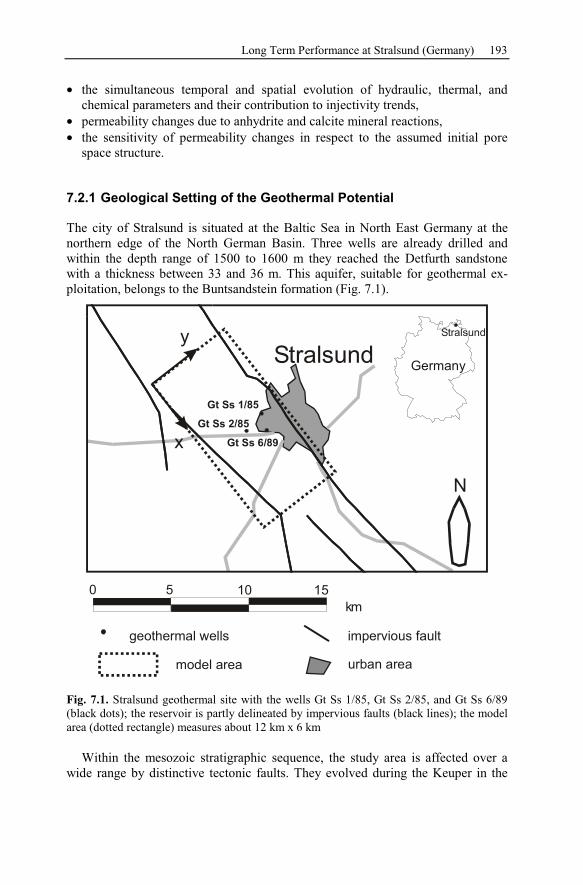
Long Term Performance at Stralsund (Germany) 193
• the simultaneous temporal and spatial evolution of hydraulic, thermal, and
chemical parameters and their contribution to injectivity trends,
• permeability changes due to anhydrite and calcite mineral reactions,
• the sensitivity of permeability changes in respect to the assumed initial pore
space structure.
7.2.1 Geological Setting of the Geothermal Potential
The city of Stralsund is situated at the Baltic Sea in North East Germany at the
northern edge of the North German Basin. Three wells are already drilled and
within the depth range of 1500 to 1600 m they reached the Detfurth sandstone
with a thickness between 33 and 36 m. This aquifer, suitable for geothermal ex-
ploitation, belongs to the Buntsandstein formation (Fig. 7.1).
N
Germany
Stralsund
Stralsund
geothermal wells impervious fault
model area
0 5 10 15
km
urban area
y
x
Gt Ss 1/85
Gt Ss 2/85
Gt Ss 6/89
Fig. 7.1. Stralsund geothermal site with the wells Gt Ss 1/85, Gt Ss 2/85, and Gt Ss 6/89
(black dots); the reservoir is partly delineated by impervious faults (black lines); the model
area (dotted rectangle) measures about 12 km x 6 km
Within the mesozoic stratigraphic sequence, the study area is affected over a
wide range by distinctive tectonic faults. They evolved during the Keuper in the
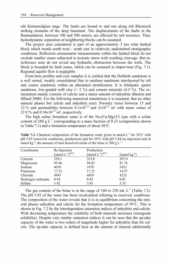
194 Reservoir Management
old Kimmeridgian stage. The faults are bound to and run along old Rheinisch
striking elements of the deep basement. The displacements of the faults in the
Buntsandstein, between 100 and 500 meters, are affected by salt tectonics. Thus,
hydrodynamic separation of neighboring blocks can be assumed.
The project area considered is part of an approximately 5 km wide faulted
block which trends north west - south east in relatively undisturbed stratigraphic
conditions. Reflection seismometer measurements within the faulted block do not
exclude smaller zones subjected to tectonic stress with resulting cleavage. But in-
terference tests do not reveal any hydraulic obstruction between the wells. The
block is bounded by fault zones, which can be assumed as impervious (Fig. 7.1).
Regional aquifer flow is negligible.
From bore profiles and core samples it is yielded that the Detfurth sandstone is
a well sorted, weakly consolidated fine to medium sandstone interlayered by silt
and coarse sandstone within an alternated stratification. It is feldspatic quartz
sandstone, low-graded with clay (< 2 %) and cement minerals (4-5 %). The ce-
mentation mainly consists of calcite and a minor amount of anhydrite (Bartels and
Iffland 2000). For the following numerical simulations it is assumed, that no other
mineral phases but calcite and anhydrite react. Porosity varies between 15 and
32 % and permeability between 0.1x10⁻¹²
and 2x10-12
m² with mean values of
23.9 % and 0.54x10⁻¹²
m², respectively.
The high saline formation water is of the Na-(Ca-Mg)-Cl type with a solute
content of 280 g L-1
corresponding to a mass fraction of 0.23 (composition shown
in Table 7.1) and a formation temperature of about 58°C.
Table 7.1. Chemical composition of the formation water given in mmol L-1
for 58°C with
pH 5.85 (reservoir conditions, production) and for 20°C with pH 5.84 (re-injection) and in
mmol kg-1
; the amount of total dissolved solids of the brine is 280 g L-1
Constituents Re-Injection
[mmol L-1
]20°C
Production
[mmol L-1
]58°C
[mmol kg-1
]
Calcium 359.1 353.0 307.0
Magnesium 95.66 94.02 81.76
Sodium 4039 3970 3452
Potassium 17.52 17.22 14.97
Chloride 4943 4859 4225
Hydrogen carbonate 0.94 0.93 0.81
Sulfate 3.92 3.85 3.35
The gas content of the brine is in the range of 180 to 250 mL L-1
(Table 7.2).
The pH 5.85 of the water has been recalculated referring to reservoir conditions.
The composition of the water reveals that it is in equilibrium concerning the min-
eral phases anhydrite and calcite for the formation temperature of 58°C. This is
shown in Fig. 7.2 by the interdependent saturation indices of anhydrite and calcite.
With decreasing temperature the solubility of both minerals increases (retrograde
solubility). Despite very similar saturation indices it can be seen that the up-take
capacity of the water is two orders of magnitude higher for anhydrite than for cal-
cite. The up-take capacity is defined here as the amount of mineral additionally
Long Term Performance at Stralsund (Germany) 195
soluble in the formation water if temperature decreases from 58°C (initial forma-
tion temperature) to a certain temperature (x-axis).
-0.25
-0.2
-0.15
-0.1
-0.05
0
0.05
20 25 30 35 40 45 50 55 60
Temperature [°C]
Satu
rati
on
in
dex
-7.0
-6.5
-6.0
-5.5
-5.0
-4.5
-4.0
-3.5
-3.0
-2.5
-2.0
Min
eral am
ou
nt
[lo
g m
ola
l]
SI - Calcite
SI - Anhydrite
soluble Calcite
soluble Anhydrite
Fig. 7.2. Interdependent saturation indices of anhydrite and calcite versus temperature and
the mineral up-take capacity of the reservoir water displaying the amounts of anhydrite and
calcite additionally soluble in the formation water due to decreasing temperature from ini-
tial formation temperature (58°C) to a certain temperature on the x-axis
Table 7.2. Total gas content of the brine is 180 – 250 mL L-1
Component Vol %
Methane 0.8
Ethane 0.18
Nitrogen 97.0 – 98.2
Carbon dioxide 0.8 – 2.2
Helium 0.30 – 0.58
7.2.2 Conceptual Model of Injection and Production Wells
The modeled horizontal area of the Stralsund location measures 12 km x 6 km and
is partly delineated by the existing impervious geological faults (Fig. 7.1). The
reservoir properties applied, taken from Bartels and Iffland (2000), are summa-
rized in Table 7.3.
A 2D simulation is carried out with a uniform thickness of the horizontal layer
of 34 m (Kühn et al. 2002a). The two drillings nearest to the town are used for
production and the third one for re-injection to minimize transport distances for
the hot water. Production rate is 50 m3 h
-1 for each production well (in heating
plants controlled by water-meter; reference conditions: 58°C, 1 bar, 280 g L-1
).
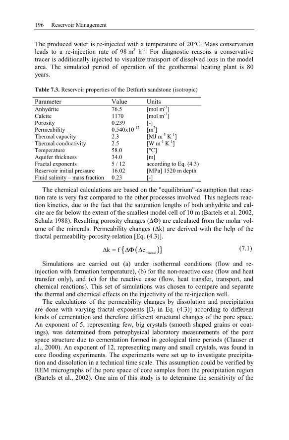
196 Reservoir Management
The produced water is re-injected with a temperature of 20°C. Mass conservation
leads to a re-injection rate of 98 m3 h
-1. For diagnostic reasons a conservative
tracer is additionally injected to visualize transport of dissolved ions in the model
area. The simulated period of operation of the geothermal heating plant is 80
years.
Table 7.3. Reservoir properties of the Detfurth sandstone (isotropic)
Parameter Value Units
Anhydrite 76.5 [mol m-3
]
Calcite 1170 [mol m-3
]
Porosity 0.239 [-]
Permeability 0.540x10⁻¹²
[m2]
Thermal capacity 2.3 [MJ m-3
K-1
]
Thermal conductivity 2.5 [W m-1
K-1
]
Temperature 58.0 [°C]
Aquifer thickness 34.0 [m]
Fractal exponents 5 / 12 according to Eq. (4.3)
Reservoir initial pressure 16.02 [MPa] 1520 m depth
Fluid salinity – mass fraction 0.23 [-]
The chemical calculations are based on the "equilibrium"-assumption that reac-
tion rate is very fast compared to the other processes involved. This neglects reac-
tion kinetics, due to the fact that the saturation lengths of both anhydrite and cal-
cite are far below the extent of the smallest model cell of 10 m (Bartels et al. 2002,
Schulz 1988). Resulting porosity changes (∆Φ) are calculated from the molar vol-
ume of the minerals. Permeability changes (∆k) are derived with the help of the
fractal permeability-porosity-relation [Eq. (4.3)].
( )}{mineral
k f c∆ = ∆Φ ∆ (7.1)
Simulations are carried out (a) under isothermal conditions (flow and re-
injection with formation temperature), (b) for the non-reactive case (flow and heat
transfer only), and (c) for the reactive case (flow, heat transfer, transport, and
chemical reactions). This set of simulations was chosen to compare and separate
the thermal and chemical effects on the injectivity of the re-injection well.
The calculations of the permeability changes by dissolution and precipitation
are done with varying fractal exponents [Df in Eq. (4.3)] according to different
kinds of cementation and therefore different structural changes of the pore space.
An exponent of 5, representing few, big crystals (smooth shaped grains or coat-
ings), was determined from petrophysical laboratory measurements of the pore
space structure due to cementation formed in geological time periods (Clauser et
al., 2000). An exponent of 12, representing many and small crystals, was found in
core flooding experiments. The experiments were set up to investigate precipita-
tion and dissolution in a technical time scale. This assumption could be verified by
REM micrographs of the pore space of core samples from the precipitation region
(Bartels et al., 2002). One aim of this study is to determine the sensitivity of the
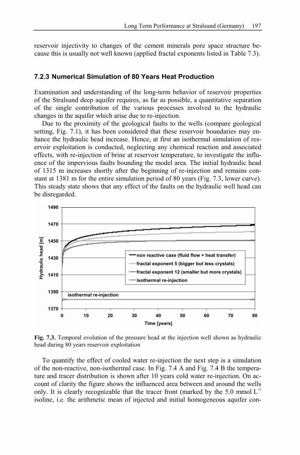
Long Term Performance at Stralsund (Germany) 197
reservoir injectivity to changes of the cement minerals pore space structure be-
cause this is usually not well known (applied fractal exponents listed in Table 7.3).
7.2.3 Numerical Simulation of 80 Years Heat Production
Examination and understanding of the long-term behavior of reservoir properties
of the Stralsund deep aquifer requires, as far as possible, a quantitative separation
of the single contribution of the various processes involved to the hydraulic
changes in the aquifer which arise due to re-injection.
Due to the proximity of the geological faults to the wells (compare geological
setting, Fig. 7.1), it has been considered that these reservoir boundaries may en-
hance the hydraulic head increase. Hence, at first an isothermal simulation of res-
ervoir exploitation is conducted, neglecting any chemical reaction and associated
effects, with re-injection of brine at reservoir temperature, to investigate the influ-
ence of the impervious faults bounding the model area. The initial hydraulic head
of 1315 m increases shortly after the beginning of re-injection and remains con-
stant at 1381 m for the entire simulation period of 80 years (Fig. 7.3, lower curve).
This steady state shows that any effect of the faults on the hydraulic well head can
be disregarded.
1370
1390
1410
1430
1450
1470
1490
0 10 20 30 40 50 60 70 80
Time [years]
Hyd
rau
lic h
ead
[m
]
non reactive case (fluid flow + heat transfer)
fractal exponent 5 (bigger but less crystals)
fractal exponent 12 (smaller but more crystals)
isothermal re-injection
isothermal re-injection
Fig. 7.3. Temporal evolution of the pressure head at the injection well shown as hydraulic
head during 80 years reservoir exploitation
To quantify the effect of cooled water re-injection the next step is a simulation
of the non-reactive, non-isothermal case. In Fig. 7.4 A and Fig. 7.4 B the tempera-
ture and tracer distribution is shown after 10 years cold water re-injection. On ac-
count of clarity the figure shows the influenced area between and around the wells
only. It is clearly recognizable that the tracer front (marked by the 5.0 mmol L-1
isoline, i.e. the arithmetic mean of injected and initial homogeneous aquifer con-
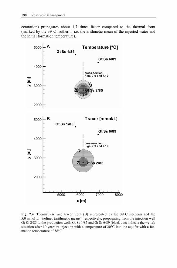
198 Reservoir Management
centration) propagates about 1.7 times faster compared to the thermal front
(marked by the 39°C isotherm, i.e. the arithmetic mean of the injected water and
the initial formation temperature).
20
39
58y
[m]
2000
3000
4000
5000
Gt Ss 2/85
cross-section
Figs. 7.9 and 7.10
Gt Ss 1/85
A Temperature [°C]
Gt Ss 6/89
5
10
x [m]
y[m
]
5000 6000 7000 8000
2000
3000
4000
5000
Gt Ss 2/85
Gt Ss 6/89
Gt Ss 1/85
B Tracer [mmol/L]
cross-section
Figs. 7.9 and 7.10
Fig. 7.4. Thermal (A) and tracer front (B) represented by the 39°C isotherm and the
5.0 mmol L-1
isolines (arithmetic means), respectively, propagating from the injection well
Gt Ss 2/85 to the production wells Gt Ss 1/85 and Gt Ss 6/89 (black dots indicate the wells);
situation after 10 years re-injection with a temperature of 20°C into the aquifer with a for-
mation temperature of 58°C
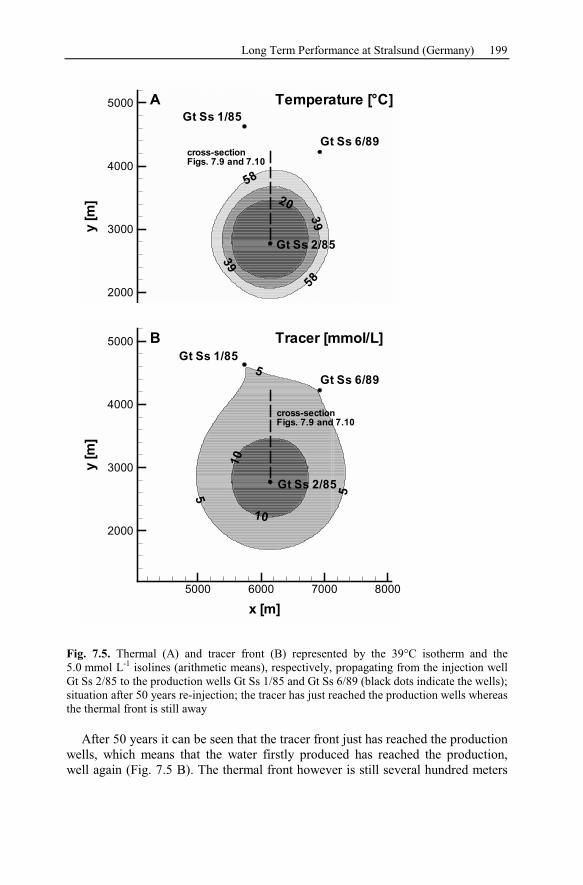
Long Term Performance at Stralsund (Germany) 199
20
39
39
58
58
y[m
]
2000
3000
4000
5000
Gt Ss 2/85
cross-section
Figs. 7.9 and 7.10
Gt Ss 1/85
A Temperature [°C]
Gt Ss 6/89
5
5
5
10
10
x [m]
y[m
]
5000 6000 7000 8000
2000
3000
4000
5000
Gt Ss 2/85
Gt Ss 6/89
Gt Ss 1/85
B Tracer [mmol/L]
cross-section
Figs. 7.9 and 7.10
Fig. 7.5. Thermal (A) and tracer front (B) represented by the 39°C isotherm and the
5.0 mmol L-1
isolines (arithmetic means), respectively, propagating from the injection well
Gt Ss 2/85 to the production wells Gt Ss 1/85 and Gt Ss 6/89 (black dots indicate the wells);
situation after 50 years re-injection; the tracer has just reached the production wells whereas
the thermal front is still away
After 50 years it can be seen that the tracer front just has reached the production
wells, which means that the water firstly produced has reached the production,
well again (Fig. 7.5 B). The thermal front however is still several hundred meters
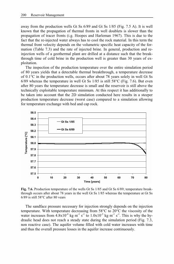
200 Reservoir Management
away from the production wells Gt Ss 6/89 and Gt Ss 1/85 (Fig. 7.5 A). It is well
known that the propagation of thermal fronts in well doublets is slower than the
propagation of tracer fronts (i.g. Hoopes and Harleman 1967). This is due to the
fact that the re-injected water always has to cool the rock material. In this term the
thermal front velocity depends on the volumetric specific heat capacity of the for-
mation (Table 7.3) and the rate of injected brine. In general, production and re-
injection wells of a geothermal plant are drilled at a distance such that the break-
through time of cold brine in the production well is greater than 30 years of ex-
ploitation.
The inspection of the production temperature over the entire simulation period
of 80 years yields that a detectable thermal breakthrough, a temperature decrease
of 0.1°C in the production wells, occurs after about 78 years solely in well Gt Ss
6/89 whereas the temperature in well Gt Ss 1/85 is still 58°C (Fig. 7.6). But even
after 80 years the temperature decrease is small and the reservoir is still above the
technically exploitable temperature minimum. At this respect it has additionally to
be taken into account that the 2D simulation conducted here results in a steeper
production temperature decrease (worst case) compared to a simulation allowing
for temperature exchange with bed and cap rock.
57.5
57.6
57.7
57.8
57.9
58.0
58.1
58.2
58.3
58.4
58.5
0 10 20 30 40 50 60 70 80
Time [years]
Tem
peratu
re [
°C
]
Gt Ss 1/85
Gt Ss 6/89
Fig. 7.6. Production temperature of the wells Gt Ss 1/85 and Gt Ss 6/89; temperature break-
through occurs after about 78 years in the well Gt Ss 1/85 whereas the temperature at Gt Ss
6/89 is still 58°C after 80 vears
The sandface pressure necessary for injection strongly depends on the injection
temperature. With temperature decreasing from 58°C to 20°C the viscosity of the
water increases from 4.8x10⁻⁴
kg m-1
s-1
to 1.0x10⁻³
kg m-1
s-1
. This is why the hy-
draulic head does not reach a steady state during the simulation period (Fig. 7.3,
non reactive case). The aquifer volume filled with cold water increases with time
and thus the overall pressure losses in the aquifer increase continuously.
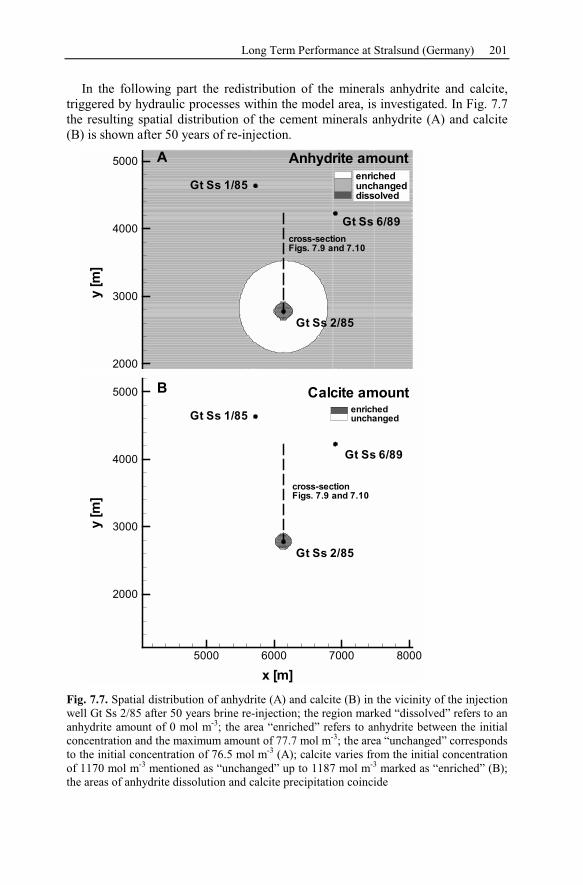
Long Term Performance at Stralsund (Germany) 201
In the following part the redistribution of the minerals anhydrite and calcite,
triggered by hydraulic processes within the model area, is investigated. In Fig. 7.7
the resulting spatial distribution of the cement minerals anhydrite (A) and calcite
(B) is shown after 50 years of re-injection.
y[m
]
2000
3000
4000
5000
77
76
Gt Ss 6/89
A Anhydrite amount
Gt Ss 2/85
Gt Ss 1/85enriched
unchanged
dissolved
cross-section
Figs. 7.9 and 7.10
x [m]
y[m
]
5000 6000 7000 8000
2000
3000
4000
5000
1170
Gt Ss 6/89
B Calcite amount
Gt Ss 2/85
Gt Ss 1/85enriched
unchanged
cross-section
Figs. 7.9 and 7.10
Fig. 7.7. Spatial distribution of anhydrite (A) and calcite (B) in the vicinity of the injection
well Gt Ss 2/85 after 50 years brine re-injection; the region marked “dissolved” refers to an
anhydrite amount of 0 mol m-3
; the area “enriched” refers to anhydrite between the initial
concentration and the maximum amount of 77.7 mol m-3
; the area “unchanged” corresponds
to the initial concentration of 76.5 mol m-3
(A); calcite varies from the initial concentration
of 1170 mol m-3
mentioned as “unchanged” up to 1187 mol m-3
marked as “enriched” (B);
the areas of anhydrite dissolution and calcite precipitation coincide
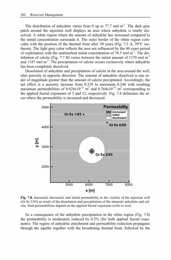
202 Reservoir Management
The distribution of anhydrite varies from 0 up to 77.7 mol m-3
. The dark gray
patch around the injection well displays an area where anhydrite is totally dis-
solved. A white region where the amount of anhydrite has increased compared to
the initial concentration surrounds it. The outer border of the white region coin-
cides with the position of the thermal front after 50 years (Fig. 7.5 A, 39°C iso-
therm). The light gray color reflects the area not influenced by the 80 years period
of exploitation with the undisturbed initial concentration of 76.5 mol m-3
. The dis-
tribution of calcite (Fig. 7.7 B) varies between the initial amount of 1170 mol m-3
and 1187 mol m-3
. The precipitation of calcite occurs exclusively where anhydrite
has been completely dissolved.
Dissolution of anhydrite and precipitation of calcite in the area around the well,
alter porosity in opposite direction. The amount of anhydrite dissolved is one or-
der of magnitude greater than the amount of calcite precipitated. Accordingly, the
net effect is a porosity increase from 0.239 to maximum 0.246 with resulting
maximum permeabilities of 0.624x10⁻¹²
m2 and 0.764x10
-12 m
2 corresponding to
the applied fractal exponents of 5 and 12, respectively. Fig. 7.8 delineates the ar-
eas where the permeability is increased and decreased.
x [m]
y[m
]
5000 6000 7000 8000
2000
3000
4000
5000
0
0
Gt Ss 6/89
Gt Ss 2/85
Gt Ss 1/85
Permeability
increased
initial
decreased
Fig. 7.8. Increased, decreased, and initial permeability in the vicinity of the injection well
(Gt Ss 2/85) as result of the dissolution and precipitation of the minerals anhydrite and cal-
cite; final permeabilities depend on the applied fractal exponents (refer to text)
As a consequence of the anhydrite precipitation in the white region (Fig. 7.8)
the permeability is moderately reduced by 0.2% (for both applied fractal expo-
nents). The region of anhydrite enrichment and permeability reduction propagates
through the aquifer together with the broadening thermal front, followed by the
Long Term Performance at Stralsund (Germany) 203
anhydrite dissolution zone. When the cooling front propagates further and the in-
jection temperature of 20°C is approached the redistributed anhydrite is dissolved
again, accompanied by calcite precipitation.
The propagating reaction fronts are shown in more detail along the cross sec-
tions in Fig. 7.9 and Fig. 7.10 as functions of distance from the injection well
Gt Ss 2/85 (x = 6140 m and y = 2775 m). Fig. 7.9 displays the distribution of pH
and dissolved calcium, sulfate, and carbonate as well as the minerals anhydrite and
calcite compared to the thermal and tracer front after a period of 10 years. The
thermal front (20°C 58°C) extends from 3100 m to 3400 m (y-axis) and the
tracer front (0 mmol kg-1
10 mmol kg-1
) from 3300 m to 3600 m. Obviously the
concentrations of solutes and minerals are closely related to the temperature dis-
tribution and transport processes. Near the injection well calcium has a concentra-
tion of 307.7 mmol kg-1
(injected conc. 306.9 mmol kg-1
), which increases to
309.4 mmol kg-1
at 2880 m. Sulfate reacts comparable to calcium with a concen-
tration of 3.35 mmol kg-1
(≡ injected conc.) increasing to 5.08 mmol kg-1
. Within
the thermal front the concentrations of calcium and sulfate decrease to 305.4 and
3.32 mmol kg-1
, respectively. Within the tracer front, intersecting the thermal
front, calcium re-increases to 306.9 mmol kg-1
whereas sulfate further declines to
3.12 mmol kg-1
. Compared to calcium and sulfate the development of the pH and
the carbonate concentration is different. pH and carbonate increase almost instan-
taneously after re-injection. The pH shifts from 5.92 (injected pH 5.84) to 5.98
and carbonate 0.84 mmol kg-1
(injected conc. 0.81 mmol kg-1
) to 0.86 mmol kg-1
.
At 2880 m the pH decreases from 5.98 to 5.97 accompanied by an increase in
carbonate from 0.86 to 0.87 mmol kg-1
. Within both the thermal and the tracer
front pH decreases to minimum 5.75 and rises again to 5.82. In contrast to pH car-
bonate increases firstly to 1.05 mmol kg-1
and decreases afterwards to 0.81
mmol kg-1
. As already shown (Fig. 7.7 A and B), anhydrite is totally dissolved in
the near vicinity of the injection well whereas calcite increased from the initial
concentration of 1170 mol m-3
to maximum 1187 mol m-3
within this area. Further
downstream from the injection well anhydrite is increased to maximum 77.7
mol m-3
curving down to the initial concentration of 76.5 mol m-3
within the ther-
mal front. Calcite remains constant with the initial concentration of 1170 mol m-3
.
Fig. 7.10 displays the same quantities as Fig. 7.9 but now after the period of 50
years. The thermal front (20°C 58°C) extends from 3500 m to 3900 m. The
tracer front already had passed the observed sector. Shapes of the distributions as
well as the concentrations of solutes and minerals after 50 years re-injection are
similar to the situation after 10 years. In difference, rise in calcium, sulfate, and
carbonate as well as decrease of pH occurs further downstream (y = 2950 m) and
re-increase of calcium behind the thermal front is small from 305.1 to 305.4
mmol kg-1
. The pH decreases from 5.98 to 5.72 within the thermal front and re-
mains constant from there on. Carbonate concentration increases from 0.88 to 1.20
mmol kg-1
and smoothly curves down to 1.17 mmol kg-1
. The region of anhydrite
dissolution, which is identical with the area of calcite increase, is enlarged as well
as the region of anhydrite increase downstream up to the thermal front.
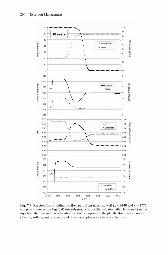
204 Reservoir Management
0
10
20
30
40
50
60
70
Tem
pera
ture
[°C
]
0
1
2
3
4
5
6
7
8
9
10
Tra
cer
[mm
ol/kg]
Temperature
Tracer
10 years
303
304
305
306
307
308
309
310
Ca
lciu
m [
mm
ol/kg
]
2
3
4
5
6
7
8
9
Su
lfa
te [
mm
ol/kg
]
Calcium
Sulfate
5.60
5.65
5.70
5.75
5.80
5.85
5.90
5.95
6.00
pH
0.70
0.75
0.80
0.85
0.90
0.95
1.00
1.05
1.10
Ca
rbo
na
te [
mm
ol/kg
]
pH
Carbonate
1100
1125
1150
1175
1200
1225
1250
2775 2975 3175 3375 3575 3775 3975 4175
y [m]
Ca
lcite
[m
ol/m
³]
72
73
74
75
76
77
78
An
hyd
rite
[m
ol/m
³]
Calcite
Anhydrite
Fig. 7.9. Reaction fronts within the flow path from injection well (x = 6140 and y = 2775,
compare cross-section Fig. 7.4) towards production wells; situation after 10 years brine re-
injection; thermal and tracer fronts are shown compared to the pH, the dissolved amounts of
calcium, sulfate, and carbonate and the mineral phases calcite and anhydrite
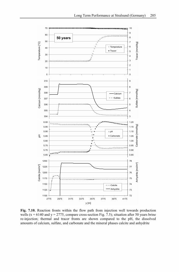
Long Term Performance at Stralsund (Germany) 205
0
10
20
30
40
50
60
70
Te
mp
era
ture
[°C
]
0
1
2
3
4
5
6
7
8
9
10
Tra
ce
r [m
mo
l/kg
]
Temperature
Tracer
50 years
304
305
306
307
308
309
310
Ca
lciu
m [
mm
ol/kg
]
3
4
5
6
7
8
9
Su
lfa
te [
mm
ol/kg
]
Calcium
Sulfate
5.65
5.70
5.75
5.80
5.85
5.90
5.95
6.00
pH
0.85
0.90
0.95
1.00
1.05
1.10
1.15
1.20
Ca
rbo
na
te [
mm
ol/kg
]
pH
Carbonate
1100
1125
1150
1175
1200
1225
1250
2775 2975 3175 3375 3575 3775 3975 4175
y [m]
Ca
lcite
[m
ol/m
³]
72
73
74
75
76
77
78
An
hyd
rite
[m
ol/m
³]
Calcite
Anhydrite
Fig. 7.10. Reaction fronts within the flow path from injection well towards production
wells (x = 6140 and y = 2775, compare cross-section Fig. 7.5); situation after 50 years brine
re-injection; thermal and tracer fronts are shown compared to the pH, the dissolved
amounts of calcium, sulfate, and carbonate and the mineral phases calcite and anhydrite
206 Reservoir Management
The temperature regime during the injection process controls the chemical reac-
tions. As anhydrite and calcite are more soluble in cold than in hot water (retro-
grade solubility, Fig. 7.2) injecting 20°C water into an aquifer with a formation
temperature of 58°C should cause dissolution of anhydrite and calcite around the
injection well. As can be seen in Fig. 7.9 and Fig. 7.10 anhydrite dissolution does
occur, but simultaneously the calcite amount in the vicinity of the well is increased
due to precipitation. Separate geochemical simulations with a box model revealed
that with the beginning of the re-injection anhydrite and calcite start to dissolve.
Due to the fact, that the uptake capacity of the geothermal brine is two orders of
magnitude higher for anhydrite if temperature decreases (Fig. 7.2) and additionally
the initial amount of anhydrite is one order of magnitude lower than the one of
calcite (Table 7.3), the depletion of anhydrite apparently proceeds at a higher rate
if unsaturated cold water passes. When anhydrite is totally dissolved the injected
brine equilibrates solely with the remaining calcite and with a slightly higher
amount than in the additional presence of dissolved anhydrite.
This injected water, now saturated with calcite (in the absence of anhydrite)
further downstream reaches areas with both, anhydrite and calcite, in the pore
space. Re-equilibration leads to dissolution of anhydrite and simultaneous precipi-
tation of calcite. As a result the calcite amount increases slightly above the initial
concentration of 1170 mol m-3
(Fig. 7.7 B, Fig. 7.9, and Fig. 7.10). That reaction
exclusively occurs at the border between the innermost region already freed from
anhydrite and the adjoining one where both minerals are still left.
Compared to the composition of the re-injected water, the mineral reactions of
anhydrite and calcite described above result in transport of increased amounts of
calcium, sulfate, and carbonate through the aquifer. The transport of dissolved
ions is faster than the propagation of the low temperature front through the aquifer
as discussed in the beginning of this section (compare Fig. 7.4, Fig. 7.5, Fig. 7.9,
and Fig. 7.10). Therefore water at 20°C in equilibrium with larger amounts of cal-
cium, sulfate, and carbonate eventually reaches the high temperature region from
upstream. Due to their retrograde solubility less anhydrite and calcite should be
soluble in the brine at the higher temperature. Hence, increased amounts of anhy-
drite are observed in the zone between the inner region where anhydrite is totally
dissolved and the outer high temperature region (Fig. 7.9 and Fig. 7.10), compared
to the initial concentration of 76.5 mol m-3
. But for calcite, contrary to the expec-
tations raised above, dissolution is indicated by decreasing pH and increasing car-
bonate concentration within the thermal front. The reason for these observations is
the interaction between solutes and minerals close to thermodynamic equilibrium.
Within the thermal front thermodynamic equilibrium is reached by precipitation of
anhydrite and simultaneous dissolution of calcite.
The pH, the concentrations of the solutes, and the temperature remain at their
natural formation values downstream of the thermal front (Table 7.1, production;
Fig. 7.9, after 10 years). After tracer breakthrough in the production well the dis-
tribution of the solutes has changed completely compared to their initial distribu-
tion, due to the chemical processes occurring at the injection well and the thermal
front and the transport of the re-equilibrated brine through the model area (Fig.
7.10, after 50 years).
Long Term Performance at Stralsund (Germany) 207
Running a Geothermal Heating Plant the most essential parameter, beside pro-
duction rate and temperature, is the injection pressure. This pressure depends on
permeability, thickness of the aquifer, temperature, and rate of re-injection. The
trend of the equivalent hydraulic head at the injection well is shown in Fig. 7.3,
which is, due to the chosen reference density (brine of 280 g L-1
), equivalent with
the well-block pressure (the computed pressure in the grid block containing the
well). The initial hydraulic head of 1315 m corresponds to the reservoir pressure
of 16.02 MPa assuming a water column of constant temperature and salinity and a
situation of no exploitation. For the non-reactive case (flow and heat transfer only)
it can be seen that the hydraulic head increases almost up to 1470 m. Even after 80
years of heat production it is not at steady state. Taking into account chemical re-
actions the hydraulic head increase rate declines. A fractal exponent of 5 repre-
sents dissolution and precipitation of natural mineral cementation with structures
formed by diagenesis (Clauser et al. 2000). The effect of reduced hydraulic head
increase is smaller with a fractal exponent 5 compared to the fractal exponent 12.
A fractal exponent of 12 represents dissolution and precipitation of many small
crystals formed in a technical time scale at comparatively rapid flow (Bartels et al.
2002). It can be seen that the mineral reactions at application of the fractal expo-
nent 12 provide an almost constant hydraulic head of 1450 meters required for re-
injection at the end of the simulation period. The hydraulic head evolution at the
injection well depends on the rate of permeability changes: the larger the fractal
exponent, the lower the resulting hydraulic head.
The occurring chemical reactions applied with the two limiting values of the
observed fractal exponents 5 and 12, cause a decrease of the hydraulic head by
about 5 % and 13 %, respectively. As a result of the mineral redistribution around
the injection well, the injectivity of the layer increases compared to the non-
reactive case of flow. Considering the injection well head pressure this could bal-
ance moderate aging trends in well injectivity observed in operating plants but not
discussed here.
In the period considered, the injectivity decrease due to the cold water viscosity
is partially or even fully compensated by the dissolution of calcite and anhydrite in
the formation. The absolute hydraulic head change due to the chemical reactions is
smaller compared to changes caused by thermal effects, but however the hydraulic
reservoir properties are improved, due to the dissolution of anhydrite around the
well, whereas the precipitation of anhydrite within the thermal front is of minor
importance concerning the injectivity of the re-injection well. The resulting net in-
crease of well injectivity is sensitive to the actual pore space structure.
7.2.4 Conclusion Drawn from the Stralsund Case Study
The numerical case study of heat exploitation for district heating is carried out for
the Stralsund location with its already confirmed geothermal potential. It is chosen
because a complete data set of the formation parameters of the Detfurth sandstone
and the high saline formation water is available. From this study focusing on in-
208 Reservoir Management
jectivity changes due to exploitation of a hydrothermal reservoir it can be con-
cluded, that:
• the evolution of the well injectivity, one of the most important technical pa-
rameter for reservoir exploitation, is influenced primarily by thermal effects, in
which the re-injection of the cooled water leads to a steady reduction of the hy-
draulic conductivity;
• mineral dissolution and precipitation of anhydrite and calcite has no negative
effect on the reservoir exploitation, but quite the reverse, well injectivity im-
proves moderately. The resulting hydraulic head decreases with up to 13 %,
compared to the non-reactive case of flow, are significant but not dominating
for the process. Nevertheless, this difference can represent a large fraction of
re-injection pressure requirement at the wellhead in cases where sandface pres-
sure has to be higher than the cold water column hydrostatic pressure;
• the chemical mineral redistribution in the aquifer weakens the viscosity induced
trend of increasing hydraulic head at the injection well;
• the pore space structure of both, the natural mineral cementation of the forma-
tion and the newly precipitated mineral, significantly determines the rate of per-
meability change due to the chemical reactions.
It can be summarized that a reservoir moderately cemented with retrograde dis-
solving minerals (here anhydrite and calcite) and with sufficient initial porosity
and permeability will require lower pressure heads for long-term re-injection
compared to a reservoir with the same initial permeability and porosity but with-
out reactive cement minerals. Hence, from the geochemical point of view the
long-term operation of a geothermal heating plant at the location Stralsund is not
restricted.
With this study, adding geochemical and complex modeling aspects, previous
studies have been completed, which have stated that the Stralsund location is suit-
able for long-term operation of a geothermal heating plant from the hydrogeologi-
cal and hydrothermal point of view. Taking into account mineral reactions and re-
sulting changes of the pore space structure and hydraulic parameters further
confirms and ensures the utilizable geothermal potential at Stralsund.
References
Abe M (1993) Long term use of acidic reservoir at Onikobe geothermal power plant. In:
Lee KC, Dunstall MG, Hochstein MP (eds) Proceedings of the 15th
New Zealand Geo-
thermal Workshop 1993 Geothermal Institute, University of Auckland, pp 193-197
Adams MC (1996) Chemistry of fluids from Ascension #1, a deep geothermal well on As-
cension Island, South Atlantic Ocean. Geothermics 25(4/5):561-579
Adams MC, Lemieux M, Moore JN, Johnson SD (1989) Fluid chemistry and hydrogeology
of the Heber geothermal system, California. Proceedings, Fourteenth Workshop on
Geothermal Reservoir Engineering Stanford University, Stanford, California, January
24-26, pp 81-86
Akaku K, Kasai K, Nakatsuka K (2000) Modeling of formation of acid water discharged
from high temperature geothermal reservoir. Proceedings of World Geothermal Con-
gress 2000, Kyushu - Tohuku, Japan, May 28 - June 10, pp 895-900
Appelo CAJ, Postma D (1999) Geochemistry, groundwater and pollution. Balkema Pub-
lishers, Rotterdam
ARC (1991) Waiwera geothermal groundwater resources statement and allocation plan.
Auckland Regional Council, Technical Publication No. 112
ARC (1999) Waiwera geothermal groundwater resource assessment report. Auckland Re-
gional Council, Technical Publication No. 115
Arihara S, Arihara N (1999) Modeling silica deposition in injection wells of the Otake geo-
thermal field, Japan. Proceedings, Twenty-Fourth Workshop on Geothermal Reservoir
Engineering, Stanford University, Stanford, California, January 25-27, 2001, pp 78-85
Ármannsson H, Kristmannsdóttir H, Ólafsson M (2000) Geothermal influence on ground-
water in the Lake Mývatn area, North Iceland. Proceedings of World Geothermal Con-
gress 2000, Kyushu - Tohuku, Japan, May 28 - June 10, pp 515-520
Arnorsson S, Gunnlaugsson E, Svavarsson H (1983) The chemistry of geothermal waters in
Iceland. II. Mineral equilibria and independent variables controlling water composi-
tions. III. Chemical geothermometry in geothermal investigations. Geochimica et
Cosmochimica Acta 42:547-566/567-577
ARWB (1980) Waiwera water resource survey – Preliminary water allocation/management
plan. Auckland Regional Water Board, Technical Publication No. 17
ARWB (1987) Waiwera thermal groundwater allocation and management plan 1986. Auck-
land Regional Water Board, Technical Publication No. 39
Back W, Hanshaw BB, Pyle TE, Plummer LN, Weidie AE (1979) Geochemical signifi-
cance of ground-water discharge and carbonate solution to the formation of Caleta Xel
Ha, Quintana Roo, Mexico. Water Resources Research 15(6):1521-1535
Baermann A, Kröger J, Taugs R, Wüstenhagen K, Zarth M (2000a) Anhydrite Cement in
Rhaetian Sandstones in Southeastern Hamburg: Morphologie and Structure. Zeitschrift
für angewandte Geologie 46(3):138-144 (in German)
Baermann A, Kröger J, Zarth M (2000b) Anhydrite Cement in Rhaetian Sandstones in
Hamburg: X-ray and NMR Tomographie Studies and Leaching Tests. Zeitschrift für
angewandte Geologie 46(3):144-152 (in German)
Michael Kuhn: LNES 103, pp. 209–226, 2004.c© Springer-Verlag Berlin Heidelberg 2004
210 References
Balanque MIRD (2000) Chemical reaction path modelling of vein mineralization in the
Tongonan geothermal field, Leyte. Proceedings of World Geothermal Congress 2000,
Kyushu - Tohuku, Japan, May 28 - June 10, pp 953-958
Baldschuhn R, Binot F, Fleig S, Kockel F(2001) Tectonic Atlas of Northwest Germany and
the German North Sea Sector – Structures, Structural Development, Palaeogeography.
Geologisches Jahrbuch, Reihe A, Heft 153
Baldwin SF (2002) Renewable energy: Progress and prospects. Physics Today 55(4):62-67
Balmes CP (2000) The geochemistry of the Mt. Balut Island geothermal prospect, Davao
del Sur, Philippines. Proceedings of World Geothermal Congress 2000, Kyushu - To-
huku, Japan, May 28 - June 10, pp 959-964
Bartels J, Iffland J (2000) Hydraulic, thermal, and mechanical behavior of geothermal aqui-
fers under exploitation: Analysis and assessment of petrographical / petrophysical and
hydrochemical data and investigations as well as simulations. Project Final Report
BMBF-0326995D, Landesamt für Umwelt, Naturschutz und Geologie Mecklenburg-
Vorpommern 64 (in German)
Bartels J, Kühn M, Clauser C (2003) Numerical simulation of reactive flow using
SHEMAT. In: Clauser C (ed) Numerical simulation of reactive flow in hot aquifers -
SHEMAT and Processing SHEMAT, Springer Publishers, Heidelberg, pp 5-74
Bartels J, Kühn M., Schneider W., Clauser C., Pape H., Meyn V., Lajczak I. (2002) Core
flooding laboratory experiment validates numerical simulation of induced permeability
change in reservoir sandstone. Geophysical Research Letters 29(9):10.1029 /
2002GL014901
Bath AH, Williamson KH (1983) Isotopic and chemical evidence for water sources and
mixing in the Cerro Pando geothermal area, Republic of Panama. Geothermics
12(2/3):177-184
Battistelli A, Calore C, Pruess K (1997) The simulator TOUGH2/EWASG for modelling
geothermal reservoirs with brines and non-condensible gas. Geothermics 26(4):437-
464
Bear J (1972) Dynamics of Fluids in Porous Media, Dover Publications, New York
Bear J (1979) Hydraulics of Groundwater. MacGraw-Hill, New York
Berner R (1980) Early diagenesis: A theoretical approach. Princeton University Press
Bethke CM (1985) A numerical model of compaction-driven groundwater flow and heat
transfer and its application to the paleohydrology of intercratonic sedimentary basins.
Journal of Geophysical Research 90(B8):6817-6828
Bethke CM (1996) Geochemical reaction modeling – Concepts and Applications. Oxford
University Press, New York – Oxford
Bethke CM, Lee MK, Quinodoz HAM, Kreiling WN (1993) Basin modeling with BASIN2.
Urbana: Univeristy of Illinois Hydrology Program
Beyene K (2000) Chemical and isotopic studies of geothermal prospects, in southern Afar
Region, Ethopia. Proceedings of World Geothermal Congress 2000, Kyushu - Tohuku,
Japan, May 28 - June 10, pp 977-983
Bischoff JL, Radtke AS, Rosenbauer RJ (1981) Hydrothermal alteration of greywacke by
brine and seawater: roles of alteration and chlorite complexing on metal solubilities at
200°C and 350°C. Economic Geology 79:659-676
Bitzer K (1999) Two-dimensional simulation of clastic and carbonate sedimentation, con-
solidation, subsidence, fluid flow, heat flow and solute transport during the formation
of sedimentary basins. Computer & Geosciences 25:431-447
Bjorlykke K, Mo A, Palm E (1988) Modelling of thermal convection in sedimentary basins
and its relevance to diagenetic reactions. Marine and Petroleum Geology 5, 338-351
Block J, Waters OB (1968) The CaSO4-Na2SO4-NaCl-H2O System at 25°C to 100°C. Jour-
nal of Chemical Engineering 13(3):336-344
Reactive Flow Modeling of Hydrothermal Systems 211
Bolt GH, Groenevelt PH (1969) Coupling phenomena as a possible cause for non-Darcian
behaviour of water in soil. Bulletin International Association Hydrology 14(2), 17-26
Bortolami GC, Cravero M, Olivero GF, Ricci B, Zuppi GM (1983) Chemical and isotopic
measurements of geothermal discharges in the Acqui Terme district, Piemont, Italy.
Geothermics 12(2/3):185-197
Boudreau BP (1997) Diagenetic models and their implementation – Modelling transport
and reactions in aquatic sediments. Springer, Berlin
Brace WF (1980) Permeability of crystalline and argillaceous rocks. International Journal
of Rock Mechanics and Mining Sciences and Geomechanics Abstracts 17:241-251
Brace WF (1984) Permeability of crystalline rocks: New in situ measurements. Journal of
Geophysical Research 89:4,327-4,330
Brown KL (1986) Gold deposition from geothermal disharges in New Zealand. Economic
Geology 81:979-983
Brown KL, Webster JG, Christenson BW (1996) Precious metal sampling at the Ohaaki
geothermal field. In: Simmons SF, Rahman MM, Watson A (eds) Proceedings of the
18th
New Zealand Geothermal Workshop 1996 Geothermal Institute, University of
Auckland, pp 169-174
Browne PRL (1978) Hydrothermal alteration in active geothermal fields. Ann. Rev. Earth
Planet. Sci. 6:229-250
Burt DM (1981) Acidity-salinity diagrams – Application to greisen and porphyry deposits.
Economic Geology 76:832-843
Butler JN (1998) Ionic Equilibrium: Solubility and pH Calculations. Wiley & Sons, New
York
Campos T (1988) Geothermal resources of El Salvador – Preliminary assessment. Geo-
thermics 17(2/3):319-332
Carman PC (1956) The Flow of Gases through Porous Media. Academic Press, New York
Cataldi R (1999) The year zero of geothermics. In: Cataldi R, Hodgson SF, Lund JW (eds)
Stories from a heated Earth. Geothermal Resources Council, Davis California USA, pp
7-17
Cataldi R, Burgassi PD (1999) Flowering and decline of thermal bathing and other uses of
natural heat in the Mediterranean area, from the birth of Rome to the end of the first
millenium. In: Cataldi R, Hodgson SF, Lund JW (eds) Stories from a heated Earth.
Geothermal Resources Council, Davis California USA, pp 147-163
Cataldi R, Hodgson SF, Lund JW (1999) Stories from a heated Earth. Geothermal Re-
sources Council, Davis California USA
Cathles LM (1981) Fluid flow and genesis of hydrothermal ore deposits. Economic Geol-
ogy 75th
Anniversary Volume:424-457
Cathles LM, Smith AT (1983) Thermal constraints on the formation of Mississippi Valley-
type lead-zinc deposits and their implications for episodic basin dewatering and deposit
genesis. Economic Geology 78:983-1002
Chapman DS, Pollack HN (1975) Global Heat Flow: A new look. Earth and Planetary Sci-
ence Letters 28:23-32
Chaturongkawanich S, Leevongchareon S (2000) The geothermal resources of Changwat
Ranong Southern Thailand. Proceedings of World Geothermal Congress 2000, Kyushu
- Tohuku, Japan, May 28 - June 10, pp 1049-1052
Cheng HP, Yeh GT (1998) Development and demonstrative application of a 3-D numerical
model of subsurface flow, heat transfer, and reactive chemical transport:
3DHYDROGEOCHEM. Journal of Contaminant Hydrology 34:47-83
Chiodini G, Comodi P, Giaquinto S (1988) Ammonia and boric acid in steam and water.
Experimental data from geothermal wells in the Phlegrean fields, Naples, Italy. Geo-
thermics 17(5/6):711-718
212 References
Christensen S, Kirsch R, Liebsch-Dörschner T, Schenck P-F (2002) Hydrogeothermal En-
ergy Use in Schleswig-Holstein (Germany) – Possibilities and Restrictions. In: Geo-
thermische Vereinigung (ed) 20 Years Deep Geothermal Energy in Germany, 7. Geo-
thermische Fachtagung, 06.11.-08.11.2002, Waren, pp 99-107 (in German)
Christenson BW, Mroczek EK, Wood CP, Arehart GB (1997) Magma-ambient production
environments: PTX constraints for paleo-fluids associated with the Ngatamariki diorite
intrusion. In: Simmons SF, Morgan OE, Dunstall MG (eds) Proceedings of the 19th
New Zealand Geothermal Workshop 1997 Geothermal Institute, University of Auck-
land, pp 87-92
Clauser C (1992) Permeability of crystalline rocks. EOS, Transactions American Geo-
physical Union 73:233,237
Clauser C (2003) Numerical Simulation of Reactive Flow in Hot Aquifers. Springer Pub-
lishers, Heidelberg
Clauser C, Pape H, Bartels J, Kühn M (2000) Simulating coupled flow, heat transport,
multi-species transport, chemical water-rock interaction and resulting changes in per-
meability for model geothermal reservoirs. In: Kümpel H-J (ed) Thermo-Hydro-
Mechanical Coupling in Fractured Rock, 3rd
Euroconference on Rock Physics and
Rock, Bad Honnef - Germany, November 14. – 18., pp 53
Cox M, Browne PRL (1991) Geochemistry of ground and thermal waters in the Ngawha
area and elsewhere in Northland, New Zealand. In: Freeston DH, Browne PRL, Scott
GL (eds) Proceedings of the 13th
New Zealand Geothermal Workshop 1991 Geother-
mal Institute, University of Auckland, pp 271-277
Craig H (1963) The isotopic geochemistry of water and carbon in geothermal areas. In:
Tongiorgi E (ed) Nuclear geology in geothermal areas. Consiglio Nazional delle Ri-
cerche, Laboratorio di Geologia Nuclear, Pias, pp 17-53
D'Amore F, Fancelli R, Caboi R (1987) Observations on the application of chemical geo-
thermometers to some hydrothermal systems in Sardinia. Geothermics 16:271-282
Darcy H (1856) Les Fontaines Publiques de la Ville de Dijon. Victor Dalmont, Paris
De Gennaro M, Ferreri M, Ghiara MR, Stanzione D (1984) Geochemistry of thermal waters
on the Island of Ischia (Campania, Italy). Geothermics 13(4):361-374
De Marsily G (1986) Quantitative Hydrogeology. Academic Press, San Diego
Debye P, Hückel E (1923) Theory of electrolyte solutions. Phys. Z. 24:185-206, 305-325.
Cited in: Matthes G (1990) The composition of groundwater – Textbook of Hydro-
geology Vol. 2, Gebrüder Bornträger, Berlin 2. Print
Dongarra G, Hauser S, Alaimo R, Carapezz M, Tonani F (1983) Hot waters on Pantelleria
Island. Geochemical features and preliminary geothermal investigations. Geothermics
12(1):49-63
Dorrington P, Brown KL (2000) Management of stibnite deposition at Ngawha. In: Sim-
mons SF, Morgan OE, Dunstall MG (eds) Proceedings of the 22nd
New Zealand Geo-
thermal Workshop 2000 Geothermal Institute, University of Auckland, pp 163-168
Durst P (2002) Geochemical modelling of Soultz-sous-Forets Hot Dry Rock test site: Cou-
pling fluid-rock interactions to heat and fluid transport. Institute of Geology, Faculty of
Science, University of Neuchatel
Edmond JM, Damm K (1983) Hot springs on the ocean floor. Scientific American 248:70-
85
Ehlers J (1993) Geological Map of Hamburg 1:25.000, Explications concerning sheet no.
2526 Allermöhe. Geologisches Landesamt Hamburg, Freie Hansestadt Hamburg (in
German)
Elder JW (1967) Transient convection in a porous medium. Journal of Fluid Mechanics
27(3):609-623
Reactive Flow Modeling of Hydrothermal Systems 213
Ellis AJ, Mahon WAJ (1964) Natural hydrothermal systems and experimental hot-
water/rock interactions. Geochimica et Cosmochimica Acta 28:1323-1357
Ellis AJ, Mahon WAJ (1967) Natural hydrothermal systems and experimental hot-
water/rock interactions (Part II). Geochimica et Cosmochimica Acta 31:519-538
Endeshaw A (1988) Current status (1987) of geothermal exploration in Ethiopia. Geother-
mics 17(2/3):477-488
Energy Information Administration (2001) Office of Integrated Analysis and Forecasting,
International Energy Outlook 2001, DOE/EIA-0484, US Department of Energy, Wash-
ington DC (http://www.eia.doe.gov/oiaf/ieo/index.html, last access 27.03.2003)
Evans DG, Nunn JA (1989) Free thermohaline convection in sediments surrounding a salt
column. Journal of Geophysical Research 94(B9):413-422
Fischedick M, Langniß O, Nitsch J (2000) After the getting off – future course of renew-
able energies. S. Hirzel Verlag, Stuttgart Leipzig (in German)
Fitts CR (2002) Groundwater Science. Academic Press, Amsterdam
Fjalov AN (1959) Termofizika porod. Gostoptechizdat (in Russian)
Fournier RO (1989) Geochemistry and dynamics of the Yellowstone National Park hydro-
thermal system. Ann. Rev. Earth Planet. Science 17:13-53
Fournier RO (1990) The interpretation of Na-K-Mg relations in geothermal waters. Geo-
thermal Resources Council TRANSACTIONS 14(Part II):1421-1425
Fournier RO, Potter RW (1979) Magnesium correction to the Na-K-Ca chemical geother-
mometer. Geochimica et Cosmochimica Acta 43:1543-1550
Fournier RO, Potter RW (1982) A revised and expanded silica (quartz) geothermometer.
Geothermal Resources Council Bulletin 11(10):3-9
Freeston DH (1995) Direct uses of geothermal energy 1995 – Preliminary review. Proceed-
ings of World Geothermal Congress 1995, Florence, Italy, May 18 - 31; pp 15-25
Freeze RA, Cherry JA (1979) Groundwater. Prentice-Hall, Englewood Cliffs
Fridleifson IB (1999) Historical aspects of geothermal utilization in Iceland. In: Cataldi R,
Hodgson SF, Lund JW (eds) Stories from a heated Earth. Geothermal Resources Coun-
cil, Davis California USA, pp 307-319
Frisch U (1993) Pre-Pleistocene. In: Ehlers J (ed) Geological Map of Hamburg 1:25.000,
Explications concerning sheet no. 2526 Allermöhe. Geologisches Landesamt Ham-
burg, Freie Hansestadt Hamburg, pp 14-27 (in German)
Fritz J (1989) Geothermal Project Bruchsal. Final Report – European Commission, Non
Nuclear Energy (in German)
Gambolatti G, Putti M, Teatini P (1996) Land subsidence. In: Singh VP (ed) Hydrology of
Disasters, Kluwer Academic Publishers, Dordrecht, pp 231-268
Gammons CH, Barnes HL (1989) The solubility of Ag2S in near-neutral aqueous sulfide
solutions at 25 to 300°C. Geochimica et Cosmochimica Acta 53:279-290
Gandino A, Piovesana, Rossi R, Zan L (1985) Preliminary evaluation of Soufrière geo-
thermal field, St. Lucia (Lesser Antilles). Geothermics 14(4):577-590
Garven G, Freeze RA (1984) Theoretical analysis of the role of groundwater flow in the
genesis of stratabound ore deposits 1. Mathematical and numerical model. American
Journal of Science 284:1085-1124
Gaupp (1991) Depositional environment and diagenesis of the Main Sandstone (Middle
Rhaetian), Thönse gasfield, Lower Saxony. Niedersächsische Akademie der Geowis-
senschaften Veröffentlichungen 6:34-48 (in German)
Gelhar LW, Axness CL (1983) Three dimensional analysis of macrodispersion in aquifers.
Water Resources Research 19(1):161-180
Gelhar LW, Welty C, Rehfeldt KR (1992) A critical review of data on field-scale disper-
sion in aquifers. Water Resources Research 28(7):1955-1974
214 References
GEO – Geothermal Education Office (2001) Geothermal Energy Introduction. Microsoft
PowerPoint presentation (http://geothermal.marin.org/index.html, last acc. 27.03.2003)
Georgieva S, Vlaskovski I (2000) Structure and geothermal potential of the Bourgas hydro-
thermal basin, Bulgaria. Proceedings of World Geothermal Congress 2000, Kyushu -
Tohuku, Japan, May 28 - June 10, pp 1151-1156
Ghomshei MM, Croft SAS, Stauder JJ (1986) Geochemical evidence of chemical equilibria
in the South Meager Creek geothermal system, British Columbia, Canada. Geother-
mics 15(1):49-61
Gianelli G, Grassi S (2001) Water-rock interaction in the active geothermal system of
Pantelleria, Italy. Chemical Geology 181:113-130
Gianelli G, Piovesana F, Quy HH (1997) A reconnaissance geochemical study of thermal
waters of south and central Vietnam. Geothermics 26(4):519-533
Gianelli G, Teklemariam M (1993) Water-rock interaction processes in the Aluto-Langano
geothermal field (Ethiopia). Journal of Volcanology and Geothermal Research 56:429-
445
Gibert JP, Jaudin F (1999) Using geothermal waters in France: The district heating system
of Chaudes-Aigues from the Middle Ages. In: Cataldi R, Hodgson SF, Lund JW (eds)
Stories from a heated Earth. Geothermal Resources Council, Davis California USA, pp
287-305
Giggenbach WF (1981) Geothermal mineral equilibria. Geochimica et Cosmochimica Acta
45:393-410
Giggenbach WF (1984) Mass transfer in hydrothermal alteration systems. Geochimica et
Cosmochimica Acta 48:2693-2711
Giggenbach WF (1987) Redox processes governing the chemistry of fumarolic gas dis-
charges from White Island, New Zealand. Applied Geochemistry 2:143-161
Giggenbach WF (1988) Geothermal solute equilibria. Derivation of Na-K-Mg-Ca indica-
tors. Geochimica et Cosmochimica Acta 52:2749-2765
Giggenbach WF, Glover RB (1992) Tectonic regime and major processes governing the
chemistry of water and gas discharges from the Rotorua geothermal field, New Zea-
land. Geothermics 21(1/2):121-140
Giggenbach WF, Gonfiantini R, Jangi BL, Truesdell AH (1983) Isotopic and chemical
compositions of Parbati Valley geothermal discharges, North-West Himalaya, India.
Geothermics 12(2/3):199-222
Giggenbach WF, LeGuern F (1976) The chemistry of magmatic gases from Erta'Ale,
Ethopia. Geochimica et Cosmochimica Acta 40:25-30
Giggenbach WF, Sheppard DS, Robinson BW, Stewart MK, Lyon GL (1995) Geochemical
structure and position of the Waiotapu geothermal field, New Zealand. Geothermics
23(5/6):599-644
Goff F, Grigsby CO, Trujillo PE, Counce D, Kron A (1981) Geology, water geochemistry
and geothermal potential of the Jemez Springs area, Canon de San Diego, New Mex-
ico. Journal of Volcanology and Geothermal Research 10:227-244
Goff F, Tully J (1994) Geothermal assessment of Archuleta county and the Pagosa Springs
aquifer, Colorado. Geothermal Resources Council TRANSACTIONS 18:191-196
Goff SJ, Goff F, Janik CJ (1992) Tecuamburro volcano, Guatemala: Exploration geother-
mal gradient drilling and results. Geothermics 21(4):483-502
Goko K (2000) Structure and hydrology of the Ogiri field, West Kirishima geothermal area,
Kyushu, Japan. Geothermics 29:127-149
Gonzalez CN (1986) Interpretation of downhole temperature survey at Waiwera thermal
area. Geothermal Institute, University of Auckland, Report no. 86.07
Grassi S, Kolios N, Mussi M, Saradeas A (1996) Groundwater circulation in the Nea Kes-
sani low-temperature geothermal field (NE Greece). Geothermics 25(2):231-247
Reactive Flow Modeling of Hydrothermal Systems 215
Grimaud D, Huang S, Michard G, Zheng K (1985) Chemical study of geothermal waters of
central Tibet (China). Geothermics 14(1):35-48
Gröber H, Erk S, Grigull U (1963) Heat transfer. Springer Publishers, Berlin (in German)
Günther A (2003a) SECTION: An AVENUE program for deriving arbitrary oriented verti-
cal cross-sections through grid-based 3-D models.
(http://arcscripts.esri.com/details.asp?dbid=12710, last access 27.03.2003)
Günther A (2003b) RESTORE: An AVENUE program for vertical restoration of geological
horizons with grid based data (http://arcscripts.esri.com/details.asp?dbid=12650, last
access 27.03.2003)
Haar L, Gallagher JS, Kell GS (1984) NBS/NRC Steamtables. Hemisphere Publishing Cor-
poration, Washington, New York, London
Hanano M, Seth MS (1995) Numerical modeling of hydrothermal convection systems in-
cluding super-critical fluid. Proceedings of World Geothermal Congress 1995, Flor-
ence, Italy, May 18 – 31, pp 1681-1668
Handford CR (1981) A process-sedimentary framework for characterizing recent and an-
cient sabkhas. Sedimentary Geology 30:255-265
Hanor JS (1987) Kilometre-scale thermohaline overturn of pore waters in the Louisiana
Gulf Coast. Nature 327:501-503
Hanshaw BB, Back W, Deike RG (1971) A geochemical hypothesis for dolomitization by
ground water. Economic Geology 66(3):710-724
Hardie LA (1996) Secular variation in seawater chemistry: An explanation for the coupled
secular variation in the mineralogies of marine limestones and potash evaporites over
the past 600 m.y. Geology 24:279-283
Hardie LA, Eugster HP (1970) The evolution of closed basin brines. Mineralogical Society
of America Special Paper 3:273-290
Harrison WJ, Tempel RN (1993) Diagenetic pathways in sedimentary basins. In: Horbury
AD, Robinson AG (eds) Diagenesis and Basin Development. American Association of
of Petroleum Geologist's Studies in Geology 36, pp 69-86
Hazen A (1911) Discussion: Dams and sand foundations: Transactions, American Society
of Civil Engineers 73:199
Hearst J, Nelson P, Paillet F (2000) Well logging for physical properties: A handbook for
geophysicists, geologists and engineers, 2nd
ed. Wiley, New York
Hedenquist JW (1990) The thermal and geochemical structure of the Broadlands-Ohaaki
geothermal system. Geothermics 19:151-185
Hedenquist JW, Henley RW (1985) Hydrothermal eruptions in the Waiotapu geothermal
system, New Zealand: Origin, breccia deposits and effect on precious metal minerali-
zation. Economic Geology 80:1640-1668
Heiken G (1982) Geology of geothermal systems. In: Edwards LM, Chilingar GV, Rieke
III HH, Fertl WH (eds) Handbook of Geothermal Energy, Gulf Publishing Company,
Houston, pp 177-217
Hemley JJ, Hostetler PB, Gude AJ, Mountjoy WT (1969) Some stability relations of
alunite. Economic Geology 64:599-612
Hemley JJ, Jones WR (1964) Chemical aspects of hydrothermal alteration with emphasis
on hydrogen metasomatism. Economic Geology 59:538-569
Henley RW, Ellis AJ (1983) Geothermal systems, ancient and modern: A geochemical re-
view. Earth Sci. Rev. 19:1-50
Hochstein MP (1990) Classification and assessment of geothermal resources. In: Dickson
MH, Fanelli M (eds) Small Geothermal Resources: A Guide to Development and
Utilization, UNITAR, New York, pp 31-57
216 References
Hochstein MP, O'Sullivan MJ, Bhadee S (1987) Modelling of San Kamphaeng geothermal
reservoir. In: Geothermal Isntitute (ed) Proceedings of the 9th
New Zealand Geother-
mal Workshop 1987 Geothermal Institute, University of Auckland, pp 159-162
Hoefner ML, Fogler HS (1988) Pore evolution and channel formation during flow and reac-
tion in porous media. AIChE Journal 34(1):45-54
Hoopes JA, Harleman DR (1967) Wastewater recharge and dispersion in porous media.
Journal of the Hydraulics Division ASCE 93 (HY5)
Huang HF, Goff F (1986) Hydrogeochemistry and reservoir model of Fuzhou geothermal
field, China. Journal of Volcanology and Geothermal Research 27:203-227
Hubbert MK (1940) The theory of ground-water motion. Journal of Geology 48:785-944
Hubbert MK (1956) Darcy's law and the field equations of the flow of underground fluids.
Transactions of the American Institute of Mining, Metallurgical, and Petroleum Engi-
neers 207:222-239
Hurter S, Haenel R (2002) Atlas of Geothermal Resources in Europe. European Commis-
sion, No. EUR 17811
Huttrer GW (2000) The status of world geothermal power generation 1995-2000. Proceed-
ings of World Geothermal Congress 2000, Kyushu - Tohuku, Japan, May 28 - June 10,
pp 23-34
Huyarkon PS, Pinder GF (1983) Computational methods in subsurface flow. Academic
Press, New York
Idris H (1994) A contribution to the hydrogeothermics of groundwater systems in Egypt.
Hydrogeothermics 15:85-111
Ingebritsen SE, Sanford WE (1998) Groundwater in Geologic Processes. Cambridge Uni-
versity Press, Cambridge
Itoi R, Fukuda M, Jinno K, Shimizu S, Tomita T (1987) Numerical analysis of the injectiv-
ity of wells in the Otake geothermal field, Japan. In: Proceedings 9th
New Zealand
Geothermal Workshop 1987, November 4–6, Geothermal Institute, University of
Auckland, Auckland, New Zealand, pp 103-108
Jaritz W (1973) Development of the salt structures of NW Germany. Geologisches
Jarhbuch A 10:1-77 (in German)
Keir RS (1980) The dissolution kinetics iof biogenic calcium carbonates in seawater. Geo-
chimica Cosmochimica Acta 44:241-252
Kharaka YK (1986) Origin and evolution of water and solutes in sedimentary basins. In:
Hydrogeology of sedimentary basins: application to exploration and exploitation,
Third Canadian / American Conference on Hydrogeology 1986, pp 173-195
Kissling WM (1997) Large scale hot plate models for the TVZ geothermal fields. In: Sim-
mons SF, Morgan OE, Dunstall MG (eds) Proceedings of the 19th
New Zealand Geo-
thermal Workshop 1997 Geothermal Institute, University of Auckland, pp 51-56
Kissling WM, Brown KL, O'Sullivan MJ, White SP, Bullivant DP (1996) Modeling chlo-
ride and CO2 chemistry in the Wairakei geothermal reservoir. Geothermics 25(3):285-
305
Konikow LF, Bredehoeft JD (1992) Groundwater models can not be validated. Advances in
Water Resources 15:75-83
Kralj P, Kralj P (2000) Overexploitation of geothermal wells in Murska Soboty, Northeast-
ern Slovenia. Proceedings of World Geothermal Congress 2000, Kyushu - Tohuku, Ja-
pan, May 28 - June 10, pp 837-842
Kristmannsdóttir H (1989) Types of scaling occurring by geothermal utilization in Iceland.
Geothermics 32:183-190
Krumbein WC, Graybill FA (1965) An introduction to statistical models in geology.
McGraw-Hill, New York
Reactive Flow Modeling of Hydrothermal Systems 217
Kühn M (1997) Successive geochemical reactions during utilization of hydrogeothermal
energy. Berichte, Fachbereich Geowissenschaften, Universität Bremen, 92 (partly in
German)
Kühn M (2003) Preferential Flow Path Development in an Anhydrite Cemented Sandstone.
In: Clauser C (ed) Numerical simulation of reactive flow in hot aquifers - SHEMAT
and Processing SHEMAT, Springer Publishers, Heidelberg, pp 231-242
Kühn M, Bartels J, Iffland J (2002a) Predicting reservoir property trends under heat
exploitation: Interaction between flow, heat transfer, transport, and chemical reactions
in a deep aquifer at Stralsund, Germany. Geothermics 31(6):725-749
Kühn M, Bartels J, Pape H, Schneider W, Clauser C (2002b) Modeling chemical brine-rock
interaction in geothermal reservoirs. In: Stober I, Bucher K (eds) Water-Rock Interac-
tion, Kluwer Academic Publishers, Dordrecht, pp 147-169
Kühn M, Chiang W-H (2003) Pre- and post processing with "Processing SHEMAT". In:
Clauser C (ed) Numerical simulation of reactive flow in hot aquifers - SHEMAT and
Processing SHEMAT, Springer Publishers, Heidelberg, pp 75-151
Kühn M, Frosch G, Kölling M, Kellner T, Althaus E, Schulz HD (1997) Laboratory ex-
periments for the investigation of barite supersaturation of thermal brines. Grund-
wasser - Zeitschrift der Fachsektion Hydrogeologie 2 (3):111-117 (in German)
Kühn M, Niewöhner C, Isenbeck-Schröter M, Schulz HD (1998) Main and minor constitu-
ents in highly saline thermal waters. Water Research 32(2):265-274
Kühn M, Schneider W (2003) Injection well with reaction kinetics. In: Clauser C (ed) Nu-
merical simulation of reactive flow in hot aquifers - SHEMAT and Processing
SHEMAT, Springer Publishers, Heidelberg, pp 253-262
Kühn M, Schneider W, Bartels J, Pape H, Clauser C (1999) Numerical simulation of
chemically induced permeability changes during heat mining in hot aquifers. In: Sim-
mons SF, Morgan OE, Dunstall MG (eds) Proceedings 21st New Zealand Geothermal
Workshop 1999, November 10–12, 1999, Auckland University, New Zealand, pp 223-
228
Kühn M, Stöfen H (2001) Reaction front fingering in anhydrite cemented sandstone. In:
Simmons S, Dunstall MG, Morgan OE (eds) Proceedings 23rd New Zealand Geother-
mal Workshop 2001, November 7–9, Auckland University, New Zealand, pp 207-212
Kühn M, Stöfen H, Schneider W (2001) Coupled flow, heat transfer, solute transport, and
chemical reactions within the thermal water reservoir Waiwera, New Zealand. In:
Seiler K-P, Wohnlich S (eds) New Approaches Characterizing Groundwater Flow,
Balkema Publishers, pp 1001-1005
Kühn M, Stöfen H, Schneider W (2002c) Estimation of subsidence processes in the vicinity
of geothermal plants, Grundwasser - Zeitschrift der Fachsektion Hydrogeologie 7(1):3-
13 (in German)
Lahsen A (1988) Chilean geothermal resources and their possible utilization. Geothermics
17:401-408
Langmuir D, Mahoney J (1984) Chemical equilibrium and kinetics of geochemical proc-
esses in groundwater studies. In: Hitchon B, Walleck EI (eds) First Canadian-
American Conference on Hydrogeology, National Water Well Association, Dublin,
Ohio, pp 69-75
Langmuir D, Melchior D (1985) The geochemistry of Ca, Sr, Ba and Ra sulfates in some
deep brines from the Palo Duro Basin, Texas. Geochimica et Cosmochimica Acta
49:2423-2432
Lapwood ER (1948) Convection of a fluid in a porous media. Proceedings Cambridge Phi-
losophical Society 44, pp 508-521
Lasaga AC (1998) Kinetic Theory in the Earth Sciences. Princeton Series in Geochemistry,
Princeton Universtiy Press, Princeton, New Jersey
218 References
Lawless JV, Bromley CJ, Leach TM, Licup AC, Cope DM, Recio CM (1983) Bacon-
Manito geothermal field: A geoscientific exploration model. In: Geothermal Isntitute
(ed) Proceedings of the 5th
New Zealand Geothermal Workshop 1983 Geothermal In-
stitute, University of Auckland, pp 97-102
Lenz G, Horn H, Kellner T (1997) Final report on geology and drilling of the bore Ham-
burg Allermöhe 1. Geothermie Neubrandenburg GmbH (in German)
Lerman A (1979) Geochemical processes: Water and sediment environments. Wiley
Li YH, Gregory S (1974) Diffusion of ions in sea water and in deep-sea sediments. Geo-
chimica et Cosmochimica Acta 38:703-714
Lichtner PC (1985) Continuum model for simultaneous chemical reactions and mass trans-
port in hydrothermal systems. Geochimica et Cosmochimica Acta 49:779-800
Lichtner PC (1996) Continuum formulation of multicomponent-multiphase reactive trans-
port. Reviews in Mineralogy and Geochemistry 34(1):83-129
Lindal B (1973) Industrial and other applications of geothermal energy. In: Armstead HCH
(ed) Geothermal Energy, UNESCO, Paris, pp 135-148
Liu Z, Sun B, Liu X (1999) Chemical dosing system at Nagqu geothermal power platn (Ti-
bet). In: Simmons SF, Morgan OE, Dunstall MG (eds) Proceedings of the 21st New
Zealand Geothermal Workshop 1999 Geothermal Institute, University of Auckland, pp
193-197
Lopez MRT, Arriaga MCS (2000) Geochemical evolution of the Los Azufres, Mexico, geo-
thermal reservoir. Part I: Water and salts. Proceedings of World Geothermal Congress
2000, Kyushu - Tohuku, Japan, May 28 - June 10, pp 2257-2260
Lowell RP, Yao Y (2002) Anhydrite precipitation and the extent of hydrothermal recharge
zones at ocean ridge crests. Journal of Geophysical Research 107(B9):2183,
doi:10.1029/2001JB001289
Lu C, Reed MH, Misra KC (1992) Zinc-lead skarn mineralization at Tin Creek, Alaska:
Fluid inclusions and skarn-forming reactions. Geochimica et Cosmochimica Acta
56:109-119
Lubimova EA (1968) Thermal history of the Earth. Geophys. Mon. Ser. 13:63-77
Lund JW, Freeston DH (2000) World-wide direct use of geothermal energy 2000. Proceed-
ings of World Geothermal Congress 2000, Kyushu - Tohuku, Japan, May 28 - June 10,
pp 1-21
Lunis BC, Breckenridge R (1991) Environmental considerations. In: Lienau PJ, Lunis BC
(eds) Geothermal Direct Use, Engineering and Design Guidebook, Geo-Heat Center,
Klamath Falls, Oregon, pp 437-445
Mahon T, Harvey C, Crosby D (2000) The chemistry of geothermal fluids in Indonesia and
their relationship to water and vapour dominated systems. Proceedings of World Geo-
thermal Congress 2000, Kyushu - Tohuku, Japan, May 28 - June 10, pp 1389-1394
Mahon WAJ (1966a) Natural hydrothermal systems and the reaction of hot water with sedi-
mentary rocks. New Zealand Journal of Science 10:206-221
Mahon WAJ (1966b) Silica in hot water discharged from drillholes at Wairakei, New Zea-
land. New Zealand Journal of Science 9:135-144
Manov GG, Bates RG, Hamer WJ, Acree SF (1943) Values of the constants in the Debye-
Hückel equation for activity coefficients. Journal of the American Chemical Society
65:1765-1767
Marini L, Bonaria V, Guidi M, Huziker JC, Ottonello G, Zuccolini MV (2000) Fluid geo-
chemistry of the Acqui Terme-Visone geothermal area (Piemont, Italy). Applied Geo-
chemistry 15:917-935
Marini L, Cioni R, Guidi M (1998) Water chemistry of San Marcos area, Guatemala. Geo-
thermics 27(3):331-360
Reactive Flow Modeling of Hydrothermal Systems 219
Marshall WI, Slusher R (1966) Thermodynamics of Calcium Sulfate Dihydrate in Aqueous
Sodium Chloride Solutions, 0-110°C. Journal of Physical Chemistry 70(12):4015-4027
Martinovic M, Milivojevic M (2000) The hydrothermal model of Macva. Proceedings of
World Geothermal Congress 2000, Kyushu - Tohuku, Japan, May 28 - June 10, pp
2145-2151
McCume CC, Forgler HS, Kline WE (1979) An experiment technique for obtaining perme-
ability-porosity relationship in acidized porous media. Ind Eng Chem. Fundam
18(2):188-192
McGuinness MJ, White SP, Young RM, Ishizaki H, Ikeuchi K, Yoshida Y (1995) A model
of the Kakkonda geothermal reservoir. Geothermics 24:1-48
Melchior DC, Bassett RL (1990) Chemical Modeling of Aqueous Systems II. ACS Sympo-
sium Series 416, American Chemical Society, Washington DC
Mercer JW, Thomas SD, Ross B (1982) Parameters and Variables Appearing in Repository
Siting Models. GeoTrans Inc., NUREG/CR-3066
Merkel (1991) Results of hydrochemical and isotopic investigations of the brines Waren
"GT/Wa 1/81" and Neubrandenburg "N 1 GT 86". WATEC Ingeieurgesellschaft,
Markt Schwaben (in German, unpublished)
Meyer C, Hemley JJ (1967) Wall rock alteration. In: Barnes HL (ed) Geochemistry of
hydrothermal ore deposits, Holt Rinehart & Winston, New York, pp 166-235
Moeller N, Weare JH, Greenberg JP, Duan Z (2000) Modeling technology for increasing
geothermal energy productivity. Proceedings of World Geothermal Congress 2000,
Kyushu - Tohuku, Japan, May 28 - June 10, pp 4059-4064
Monnin C, Ramboz C (1996) The anhydrite saturation index of the ponded brines and
sediment pore waters of the Red Sea deeps. Chemical Geology 153:187-209
Moon BR, Dharam P (1988) Geothermal energy in India: Present Status and future pros-
pects. Geothermics 17(2/3):439-449
Morse JW (1983) The kinetics of calcium carbonate dissolution and precipitation. In:
Reeder RJ (ed) Reviews in Mineralogy, American Minerlogical Society 11:227-264
Mroczek EK, White SP, Graham D (2000) Deposition of silica in porous packed beds - Pre-
dicting the lifetime of reinjection aquifers. Geothermics 29:737-757
Mroczek EK, White SP, Graham D (2002) Estimating the quantity of silica deposited in the
reservoir around an injection well. In: Soengkono S, Browne PRL (eds) Proceedings of
the 24th
New Zealand Geothermal Workshop 2002 Geothermal Institute, University of
Auckland, pp 187-190
Mroczek EK, White SP, Graham DJ (1999) Comparison of amorphous silica deposition
rates measured using packed pipes and a fluidised bed at FP10, Wairakei. In: Simmons
SF, Morgan OE, Dunstall MG (eds) Proceedings 21st New Zealand Geothermal Work-
shop 1999, November 10–12, 1999, Auckland University, New Zealand, pp 67-71
Muffler LJP (1985) Geothermal energy and geothermal resources of hydrothermal convec-
tion systems. In: Englewood CNJ (ed) Energy: For ourselves and our prosperity, Pren-
tice Hall, pp 188-207
Müller EP, Papendieck G (1975) Distribution, genesis and dynamic of deep-seated waters
under special consideration of the Zechstein. Zeitschrift geologischer Wissenschaften
3(2):167-196 (in German)
Nicholson K (1993) Geothermal Fluids – Chemistry and Exploration Techniques. Springer
Verlag, Berlin
Nieva D, Verma MP, Santoyo E, Portugal E, Campos A (1997) Geochemical exploration of
the Chipilapa geothermal field, El Salvador. Geothermics 26(5/6):589-612
Nitzsche O, Meinrath G, Merkel B (2000) Database uncertainty as a limiting factor in reac-
tive transport prognosis. Journal of Contaminant Hydrology 44:223-237
220 References
Noda T, Shimada K (1993) Water mixing model calculation for evaluation of deep geo-
thermal water. Geothermics 22(3):165-180
Nordstrom DK, Ball JW (1984) Chemical models, computer programs and metal complexa-
tion in natural water. In: Kramer CJM, Duniker J (eds) International Symposium on
Trace Metal Complexation in Natural Water. Martinus Nijhoff/Dr J.W. Junk Publish-
ing Co, pp 149-169
Norton D, Knight J (1977) Transport phenomena in hydrothermal systems: Cooling plu-
tons. American Journal of Science 277:937-981
O’Sullivan M, Pruess K, Lippmann MJ (2001) State of the art of geothermal reservoir
simulation. Geothermics 30:395-429
Olivella S, Carrera J, Gens A, Alonso EE (1996) Porosity variations in saline media caused
by temperature gradients coupled to multiphase flow and dissolution/precipitation.
Transport in Porous Media 25:1-25
Oliver J (1986) Fluids expelled tectonically from orogenic belts: Their role in hydrocarbon
migration and other geologic phenomena. Geology 14:99-102
Ormond A, Ortoleva P (2000) Numerical modeling of reaction-induced cavities in a porous
rock. Journal of Geophysical Research 105(B7):16,737-16,747
Ortoleva P, Chadam J, Merino E, Sen A (1987) Geochemical self-organization II: The reac-
tive-infiltration instability. American Journal of Science 287:1008-1040
Ortoleva PJ (1994) Geochemical Self-Organization. Oxford Monographs on Geology and
Geophysics Vol. 23, Oxford University Press, New York
Özgüler ME, Kasap A (1999) The geothermal history of Anatolia, Turkey. In: Cataldi R,
Hodgson SF, Lund JW (eds) Stories from a heated Earth. Geothermal Resources Coun-
cil, Davis California USA, pp 51-67
Pandey OMP (1982) Terrestrial heat flow in New Zealand. Victoria University of Welling-
ton, New Zealand, Ph.D. thesis (unpublished)
Pape H, Clauser C, Iffland J (1999) Permeability prediction for reservoir sandstones based
on fractal pore space geometry. Geophysics 64(5):1447-1460
Parkhurst DL, Appelo CAJ (1999) User's guide to PHREEQC (version 2)--A computer
program for speciation, batch-reaction, one-dimensional transport, and inverse geo-
chemical calculations: U.S. Geological Survey Water-Resources Investigations Report
99-4259
Paschke SS, van der Heijde P (1996) Overview of chemical modeling in groundwater and
listing of available geochemical models. International Groundwater Modeling Center,
Report GWMI-96-01, Golden Co., Colorado School of Mines
Pham M, Klein C, Sanyal S, Xu T, Pruess K (2001) Reducing cost and environmental im-
pact of geothermal power through modeling of chemical processes in the reservoir.
Proceedings, Twenty-Sixth Workshop on Geothermal Reservoir Engineering, Stanford
University, Stanford, California, January 29-31, 2001, SGP-TR-168, pp 216-223
Phillips OM (1991) Flow and reaction in permeable rocks. Cambridge University Press,
New York
Phutela RC, Pitzer KS (1986) Thermodynamics of electrolyte mixtures. Enthalpy and the
effect of temperature on the activity coefficient. Journal of Solution Chemistry 15:649
Piper AM (1944) A graphical procedure in the geochemical interpretation of water-
analyses. American Geophysical Union Transactions 25:914-923
Pirajno F (1992) Hydrothermal mineral deposits – Principles and fundamental concepts for
the exploration geologist. Springer Verlag, Berlin Heidelberg New York
Pitzer KS (1973) Thermodynamics of electrolytes. 1. Theoretical basis and general equa-
tions. J. Physical Chemistry 77:268-277
Pitzer KS (1975) Thermodynamics of electrolytes. V. Effects of higher-order electrostatic
terms. Journal of Solution Chemistry 4(3):249-265
Reactive Flow Modeling of Hydrothermal Systems 221
Pitzer KS (1991) Ion interaction approach: Theory and data correlation. In: Pitzer KS (ed)
Activity Coefficients in Electrolyte Solutions, CRC Press Boca Raton, 2nd Edition, pp
76-153
Pitzer KS, Kim JJ (1974) Thermodynamics of electrolytes. IV. Activity and osmotic coeffi-
cient for mixed electrolytes. Journal of American Chemical Society 96(18):5701-5707
Pitzer KS, Mayorga G (1973) Thermodynamics of electrolytes. II. Activity and osmotic co-
efficient for strong electrolytes with one or both ions univalnet. Journal of Physical
Chemistry 77(19):2300-2308
Pitzer KS, Mayorga G (1974) Thermodynamics of electrolytes. III. Activity and osmotic
coefficients for 2-2 electrolytes. Journal of Solution Chemistry 3(7):539-546
Pitzer KS, Silvester LF (1976) Thermodynamics of electrolytes. VI. Weak electolytes in-
cluding H3PO4. Journal of Solution Chemistry 5(4):269-277
Plumlee GS (1994) Fluid chemistry evolution and mineral deposition in the Main-Stage
Creede epithermal system. Economic Geology 89:1860-1882
Plumlee GS, Goldhaber MB, Rowan EL (1995a) The potential role of magmatic gases in
the genesis of Illinois-Kentucky fluorspar deposits: Implications from chemical reac-
tion path modeling. Economic Geology 90:999-1011
Plumlee GS, Leach DL, Hofstra AH, Landis GP, Rowan EL, Viets JG (1995b) Reaction
path modeling of ore deposition in Mississippi-Valley-Type Pb-Zn deposits of the
Ozark region, U.S. Midcontinent. Economic Geology 89:1361-1383
Pollack HN, Hurter SJ, Johnson JR (1993) Heat flow from the Earth's interior: Analysis of
the global data set. Reviews of Geophysics 31:267-280
Popper K (1959) The logic of scientific discovery. Harper and Row, New York
Pottorf RJ, Barnes HL (1983) Mineralogy, geochemistry and ore genesis of hydrothermal
sediments from Atlantis II Deep, Red Sea. Economic Geology Monographs 5:198-223
Praserdvigai S (1987) Geothermal development in Thailand. Geothermics 16, 565-585
Prol-Ledesma RM, Hernandez-Lombardini SI, Lozano-Santa Cruz R (1995) Chemical
variations in the rocks of La Primavera geothermal field (Mexico) related with hydro-
thermal alteration. In: Hochstein MP (ed) Proceedings of the 17th New Zealand Geo-
thermal Workshop 1995 Geothermal Institute, University of Auckland, pp 47-53
Pruess K (1991) TOUGH2 - A general-purpose numerical simulator for multiphase fluid
and heat flow, Rep. LBL-29400, Lawrence Berkeley Lab., Berkeley, California
Pruess K, Oldenburg C, Moridis G (1999) TOUGH2 – User's guide, Version 2.0. Rep.
LBL-43134, Lawrence Berkeley Lab., Berkeley, California
Pytkowicz RM (1983) Equilibria, nonequilibria and natural waters. John Wiley & Sons,
New York
Raffensberger JP, Garven G (1995a) The formation of unconformity-type uranium ore de-
posits 1. coupled groundwater flow and heat transport modeling. American Journal of
Science 295(5):581-636
Raffensberger JP, Garven G (1995b) The formation of unconformity-type uranium ore de-
posits 2. Coupled hydrochemical modeling. American Journal of Science 295:639-696
Raffensberger JP, Vlassopoulos D (1999) The potential for free and mixed convection in
sedimentary basins. Hydrogeology Journal 7:505-520
Ramirez AH (1988) Present status of geothermal reconnaissance studies in the Republic of
Panama. Geothermics 17(2/3):355-367
Reed MH (1982) Calculation of multicomponent chemical equilibria and reaction processes
in systems involving minerals, gases and aqueous phase. Geochimica et Cosmochimica
Acta 46(4):513-528
Reed MH (1983) Seawater-basalt reaction and the origin of Greenstones and related ore de-
posits. Economic Geology 78:466-485
222 References
Reed MH, Spycher N (1984) Calculation of pH and miineral equilibria in hydrothermal wa-
ters with application to geothermometry and studies of boiling and dilution. Geo-
chimica et Cosmochimica Acta 48:1479-1492
Reyes A, Giggenbach WF, Salera JRM, Salonga ND, Vergara MC (1993) Petrology and
geochemistry of Alto Peak, a vapor-cored hydrothermal system, Leyte Province, Phil-
ippines. Geothermics 22(5/6):479-519
Reyes AG, Giggenbach WF (1999) Condensate-formation and cold water incursion in the
Poihipi sector, Wairakei geothermal system. In: Simmons SF, Morgan OE, Dunstall
MG (eds) Proceedings of the 21st New Zealand Geothermal Workshop 1999 Geother-
mal Institute, University of Auckland, pp 29-36
Rickard D, Sjöberg EL (1983) Mixed kinetic control of calcite dissolution rates. American
Journal of Science 283:815-830
Rockel I (1986) Taking the waters. Early spas in New Zealand. Government Printing Office
Publishing
Rose WI, Chuan RL, Giggenbach WF, Kyle PR, Symonds RB (1986) Rates of sulfur diox-
ide emissions from White Island volcano, New Zealand, and an estimate of the total
flux of major gaseous species. Bulletin of Volcanology 48:181-188
Rougerie F, Andrié C, Jean-Baptiste P (1991) Helium-3 inside atoll barrier reef interstitial
water : A clue for geothermal endoupwelling. Geophys. Res. Letters 18:109-112
Sanford WE, Konikow LF (1989a) Simulation of calcite dissolution and porosity changes
in salt water mixing zones in coastal aquifers. Water Resources Research 25:655-667
Sanford WE, Konikow LF (1989b) Porosity development in coastal carbonate aquifers. Ge-
ology 17:249-252
Saripalli KP, Meyer PD, Bacon DH, Freedman VL (2001) Changes in hydrologic properties
of aquifer media due to chemical reactions: A Review. Critical Reviews in Environ-
mental Science and Technology 31(4):311-349
Sasada M, Doi N, Muffler LJP, Hedenquist JW (1998) Special Issue: Deep geothermal sys-
tems Japanese National project at Kakkonda. Geothermics 27(5/6):505-721
Satman A, Ugur Z, Onur M (1999) The effect of calcite deposition on geothermal well in-
flow performance. Geothermics 28:425-444
Saunders JA, Schoenly PA (1995) Boiling, colloid nucleation and aggregation, and the
genesis of bonanza Au-Ag ores of the Sleeper deposit, Nevada. Mineralium Deposita
30:199-210
Saxena VK, Gupta ML (1985) Aquifer chemistry of thermal waters of the Godavari Valley,
India. Journal of Volcanology and Geothermal Research 25:181-191
Saxena VK, Gupta ML (1987) Geochemistry of the thermal waters of Salbardi and Ta-
tapani, India. Geothermics 16:705-716
Schack A (1953) The industrial heat transfer. Steel and Iron, Düsseldorf (in German)
Schechter RS, Gidley JL (1969) The change in pore size distribution from surface reaction
in porous media. AIChE Journal 15(3):339-350
Scheidegger AE (1961) General theory of dispersion in porous media. Journal of Geophysi-
cal Research 66:3,273-3,278
Schellschmidt R, Clauser C, Sanner B (2000) Geothermal energy use in Germany at the
turn of the millennium. Proceedings of World Geothermal Congress 2000, Kyushu -
Tohuku, Japan, May 28 - June 10, pp 427-432
Schenberger DM, Barnes HL (1989) The solubility of gold in aqueous sulfide solution from
150 to 300°C. Geochimica et Cosmochimica Acta 53:269-278
Schildknecht F, Schneider W (1987) About the validity of Darcy's law under low hydraulic
gradients in sediments characterized by cohesion. Geologisches Jahrbuch, Reihe C,
Heft 48 (in German)
Reactive Flow Modeling of Hydrothermal Systems 223
Schmitz J, Flixeder F (1993) Structure of a classic chalk oil field and production enhance-
ment by horizontal drilling, Reitbrook, NW Germany. In: Spencer AM (ed) Genera-
tion, Accumulation and Production of Europe's Hydrocarbons III, Special Publication
of the European Association of Petroleum Geoscientists No. 3, pp 141-154
Schroeder JA, Purser BA (1986) Reef Diagenesis. Springer Verlag, New York
Schulz (1988) Laboratory measurments of the saturation length as a measure of the solubil-
ity kinetic of carbonates in groundwater. Geochimica et Cosmochimica Acta 52:2651-
2657 (in German)
Sekioka M (1999) Japanese geothermal waters throughout history. In: Cataldi R, Hodgson
SF, Lund JW (eds) Stories from a heated Earth. Geothermal Resources Council, Davis
California USA, pp 393-405
Severne CM (1998) Recent geochemical investigations of the Tokaanu-Waihi geothermal
field. In: Simmons SF, Morgan OE, Dunstall MG (eds) Proceedings of the 20th
New
Zealand Geothermal Workshop 1998 Geothermal Institute, University of Auckland, pp
251-257
Severne CM (1999) Traditional use of geothermal resources by New Zealand Maori. In:
Cataldi R, Hodgson SF, Lund JW (eds) Stories from a heated Earth. Geothermal Re-
sources Council, Davis California USA, pp 435-449
Seyfried WE, Bischoff JL (1981) Experimental seawater-basalt interaction at 300°C, 500
bars; chemical change, secondary mineral formation and implications for the transport
of heavy metals. Geochimica et Cosmochimica Acta 45:135-147
Shanker R, Absar A, Srivasta GC, Bajpai IP (2000) Tapoban hot water system, NW Hima-
laya, India – A unique example of heating under normal gradient conditions. In: Sim-
mons SF, Morgan OE, Dunstall MG (eds) Proceedings of the 22nd
New Zealand Geo-
thermal Workshop 2000 Geothermal Institute, University of Auckland, pp 9-12
Sheppard DS, Giggenbach WF (1980) Chemistry of the well discharges at Ngawha. In:
Geothermal Institute (ed) Proceedings of the 2nd
New Zealand Geothermal Workshop
1980 Geothermal Institute, University of Auckland, pp 91-95
Sheppard DS, Mroczek EK (2002) CO2 fluxes from geothermal systems: Assessing the ef-
fects of exploitation, and the carbon tax implications. In: Soengkono S, Browne PRL
(eds) Proceedings of the 24th
New Zealand Geothermal Workshop 2002 Geothermal
Institute, University of Auckland, pp 17-21
Sibson RH, Moore JM, Rankin AH (1975) Seismic pumping – a hydrothermal fluid trans-
port mechanism. Journal of the Geological Society London 131:653-659
Simmons SF, Browne PRL (2000) Hydrothermal minerals and precious metals in the
Broadlands-Ohaaki geothermal system: Implications for understanding low-sulfidation
epithermal environments. Economic Geology 95:971-999
Simsek S (1985) Geothermal model of Denizli, Sarayköy – Buldan area. Geothermics
14:393-417
Sjöberg EL (1978) Kinetics and mechanism of calcite dissolution in aqueous solutions at
low temperatures. Stockholm Contribution Geology XXXII, 1, pp 1-92
Soler JM, Lasaga AC (1998) An advection-dispersion-reaction model for bauxite forma-
tion. Journal of Hydrology 209:311-330
Sorey ML (1978) Numerical modeling of liquid geothermal systems. U.S. Geological Sur-
vey Professional Paper 1044-D
Sorey ML, Covard EM (1997) Hydrologic investigations in the Mammoth Corridor, Yel-
lowstone National Park and vicinity, U.S.A. Geothermics 26(2):221-249
Sorey ML, Suemnicht GA, Sturchio NC, Nordquist GA (1991) New evidence on the hydro-
thermal system Long Valley caldera, California, from wells, fluid sampling, electrical
geophysics, and age determinations of hot-spring deposits. Journal of Volcanology and
Geothermal Research 48:229-263
224 References
Spencer RJ, Eugster HP, Jones BF (1985b) Geochemistry of Great Salt Lake, Utah, II:
Pleistocene-holocene evolution. Geochimica et Cosmochimica Acta 49:739-747
Spencer RJ, Eugster HP, Jones BF, Rettig SL (1985a) Geochemistry of Great Salt Lake,
Utah, I: Hydrochemistry since 1850. Geochimica et Cosmochimica Acta 49:727-737
Spycher N, Reed MH (1992) Users guide for CHILLER: A program for computing water-
rock interactions, boiling, mixing and other reaction processes in aqueous-mineral-gas
systems. University of Oregon, Eugene, Oregon
Spycher NF, Reed MH (1989) Evolution of a Broadlands-type epithermal ore fluid along
alternative P-T paths: Implications for the transport and deposition of base, precious
and volatile metals. Economic Geology 84:328-359
Steefel CI, Lasaga AC (1990) Evolution of dissolution patterns – Permeability change due
to coupled flow and reaction. In: Melchior DC, Bassett RL (eds) ACS Symposium Se-
ries, Chemical Modeling of Aqueous Systems II, No. 416, Chap. 2, American Chemi-
cal Society, Washington DC, pp 213-225
Stöfen H (2000) Development of a heat transfer and solute transport model as a tool for
sustainable management of the thermal water resource Waiwera, New Zealand. Master
thesis, Technische Universität Hamburg-Harburg (unpublished)
Stöfen H, Kühn M (2003) Waiwera Coastal Geothermal System. In: Clauser C (ed) Nu-
merical simulation of reactive flow in hot aquifers - SHEMAT and Processing
SHEMAT, Springer Publishers, Heidelberg, pp 297-316
Stöfen H, Kühn M, Schneider W (2000) A heat transfer and solute transport model as a tool
for sustainable management of the geothermal reservoir Waiwera, New Zealand. In:
Simmons SF, Morgan OE, Dunstall MG (eds) Proceedings of the 22nd
New Zealand
Geothermal Workshop 2000 Geothermal Institute, University of Auckland, pp 273-278
Stumm W, Morgan JJ (1996) Aquatic Chemistry – Chemical Equilibria and Rates in Natu-
ral Waters. John Wiley & Sons, New York
Sunaryo D, Hantono S, Ganda, Nugroho (1993) Exploration results of the Ulubelu geo-
thermal prospect, South Sumatra, Indonesia. In: Lee KC, Dunstall MG, Hochstein MP
(eds) Proceedings of the 15th
New Zealand Geothermal Workshop 1993 Geothermal
Institute, University of Auckland, pp 103-106
Sundhoro H, Nasution A, Simanjuntak (2000) Sembalun Bumbung geothermal area, Lom-
bok Island, West Nusatenggara, Indonesia: An integrated exploration. Proceedings of
World Geothermal Congress 2000, Kyushu - Tohuku, Japan, May 28 - June 10, pp
1785-1790
Svalova VB (1999) Geothermal legends through history in Russia and the former USSR:
Abridge to the past. In: Cataldi R, Hodgson SF, Lund JW (eds) Stories from a heated
Earth. Geothermal Resources Council, Davis California USA, pp 337-355
Svanbjörnsson A, Matthíasson J, Frímannsson H, Arnórsson S, Björnsson S, Stefánsson V,
Saemundsson K (1983) Overview of geothermal development at Olkaria in Kenya.
Proceedings Ninth Workshop Geothermal Reservoir Engineering Stanford University,
Stanford, California, December 1983, SGP-TR-74, pp 65-71
Swartzendruber D (1962) Non-Darcy flow behaviour in liquid-saturated porous media.
Journal Geophysical Research 67:5205-5213
Szita G, Kocsis E (2000) How to do geothermal projects in Hungary? Dreams and realities.
Proceedings of World Geothermal Congress 2000, Kyushu - Tohuku, Japan, May 28 -
June 10, pp 3573-3578
Taylor HP (1983) Oxygen and hydrogen isotope studies of hydrothermal interactions at
submarine and subaerial spreading centers. In: Rona PA, Bostrom K, Laubier L, Smith
KL (eds) Hydrothermal processes at seafloor spreading centers. Plenum, New York, pp
83-140
Reactive Flow Modeling of Hydrothermal Systems 225
Taylor SR (1964) Abundance of chemical elements in the continental crust, a new table.
Geochimica et Cosmochimica Acta 28:1273-1285
Thomas DM (1986) Geothermal resources assessment in Hawaii. Geothermics 15(4):435-
514
Titley SR (1990) Evolution and style of fracture permeability in intrusion-centered hydro-
thermal systems. In: Bredehoeft JD, Norton DL (eds) The role of Fluids in Crustal
Processes. National Academy Press, Washington DC, pp 50-63
Tole MP (1988) Low enthalpy geothermal system in Kenya. Geothermics 17(5/6):777-783
Topinka (1997) Active Volcanoes and Plate Tectonics, "Hot Spots" and the "Ring of Fire".
USGS/CVO (http://vulcan.wr.usgs.gov/Imgs/Gif/PlateTectonics/Maps/, last access
27.03.2003)
Traganos G, Jux U, Steuber T (1995) Isotopic characteristics of geothermal waters and fos-
sil spring deposits in Mygdonia basin, Northern Greece. Geothermics 24(1):61-80
Truesdell AH (1976) Summary of section III geochemical techniques in exploration. In:
Proceedings Second United Nations Symposium on the Development and Use of Geo-
thermal Resources, San Francisco, 1975, 1, pp 1iii-1xxxix
Van der Lee J, De Windt L (2001) Present state and future directions of modeling of geo-
chemistry in hydrogeological systems. Journal of Contaminant Hydrology 47:265-282
Walter AL, Frind EO, Blower DW, Ptacek CJ, Molson JW (1994) Modeling of multicom-
ponent reactive transport in groundwater. 1. Model development and evaluation. Water
Resources Research 30:3137-3148
Wang HF, Anderson MP (1982) Introduction to groundwater modeling: Finite difference
and finite element methods. W.H. Freeman Company, San Francisco
Ward RF, Kendall CGStC, Harris PM (1986) Late permian (Guadalupian) facies and their
association with hydrocarbons. American Association of Petroleum Geologists Bulle-
tin 70:239-262
Warren JK (1989) Evaporite Sedimentology. Prentice Hall, Englewood Cliffs, New Jersey
Warren JK, Kendall GCStC (1985) Comparison of marine sabkhas (subaerial) and salina
(subaqueous) evaporites: Modern and ancient. American Association of Petroleum
Geologists Bulletin 69:1013-1023
Weeber JH, Brown LJ, White PA, Russell WJ, Thorpe HR (2001) A history of groundwater
development in New Zealand. In: Rosen MR, White PA (eds) Groundwaters of New
Zealand, New Zealand Hydrological Society, The Caxton Press, Christchurch, New
Zealand, pp 5-44
Wei C, Ortoleva P (1990) Reaction front fingering in carbonate-cemented sandstones.
Earth-Science Rev 29:183-198
Weir GJ, White SP (1996) Surface deposition from fluid flow in a porous medium. Trans-
port in Porous Media 25:79-96
White A (1986) Chemical and isotopic characteristics of fluids within the Baca geothermal
reservoir, Valles Caldera, New Mexico. Journal of Geophysical Research 91:1855-
1866
White AF, Peterson ML (1991) Chemical equilibrium and mass balance relationships asso-
ciated with the Long Valley hydrothermal system, California, U.S.A. Journal of Vol-
canology and Geothermal Research 48:283-302
White DE (1981) Active geothermal systems and hydrothermal ore deposits. Economic
Geology 75:392-423
White DE (1992) The Beowawe Geysers, Nevada, before geothermal development. US
Geological Survey Bulletin 1998
White SP (1995) Multiphase non-isothermal transport of systems of reacting chemicals.
Water Resources Research 31(7):1761-1772
226 References
White SP, Christenson BW (2000) Modelling the alteration halo of a diorite intrusion. Pro-
ceedings of World Geothermal Congress 2000, Kyushu - Tohuku, Japan, May 28 -
June 10, pp 3969-3974
White SP, Christenson BW (2002) Modelling two-phase flow above a diorite intrusion. In:
Soengkono S, Browne PRL (eds) Proceedings of the 24th
New Zealand Geothermal
Workshop 2002 Geothermal Institute, University of Auckland, pp 97-102
White SP, Mroczek EK (1998) Permeability changes during the evolution of a geothermal
field due to dissolution and precipitation of quartz. Transport in Porous Media 33:81-
101
White WB (1988) Geomorphology and Hydrology of Karst Terrain. Oxford University
Press, New York
Wolery TJ, Daveler SA (1992) EQ6, a computer program for reaction path modeling of
aqueous geochemical systems: theoretical manual, user's guide, and related documen-
tation. Lawrence Livermore National Laboratory
Wolery TJ, Jackson KJ (1990) Activity coefficients in aqueous salt solutions. In: Melchior
DC, Bassett RL (eds) ACS Symposium Series, Chemical Modeling of Aqueous Sys-
tems II, No. 416, Chap. 2, American Chemical Society, Washington DC, pp 16-29
Wood CP, Mroczek EK, Carey BS (1997) The boundary of Wairakei geothermal field: Ge-
ology and chemistry. In: Simmons SF, Morgan OE, Dunstall MG (eds) Proceedings of
the 19th
New Zealand Geothermal Workshop 1997 Geothermal Institute, University of
Auckland, pp 25-30
Wood JR, Hewett TA (1982) Fluid convection and mass transfer in porous snadstones – a
theoretical model. Geochimica et Cosmochimica Acta 46:1707-1713
Wurster P (1965) Crustal movement, sea level fluctuation, and climatic change in the Ger-
man Triassic times. Geologische Rundschau 54:224-240 (in German)
Xu M, Eckstein Y (1997) Statistical analysis of the relationships between dispersivity and
other physical properties of porous media. Hydrogeology Journal 5(4):4-20
Xu T, Pruess K (2001) On fluid flow and mineral alteration in fractured caprock of mag-
matic hydrothermal systems. Journal Geophysical Research 106 (B2):2121-2138
Yusa Y, Ohsawa S (2000) Age of the Beppu hydrothermal system, Japan. Proceedings of
World Geothermal Congress 2000, Kyushu - Tohuku, Japan, May 28 - June 10, pp
3005-3008
Zarrouk SJ, O’Sullivan MJ (2001) The effect of chemical reactions on the transport proper-
ties of porous media. In: Simmons S., Dunstall M.G., Morgan O.E. (eds) Proceedings
23rd New Zealand Geothermal Workshop 2001, November 7–9, Auckland University,
New Zealand, pp 231-236
Zhonghe P (2000) Isotope geochemistry of geothermal waters in Northern North China ba-
sin: Implications on deep fluid migration. Proceedings of World Geothermal Congress
2000, Kyushu - Tohuku, Japan, May 28 - June 10, pp 1559-1564
Zhu C, Anderson G (2002) Environmental Applications of Geochemical Modeling. Cam-
bridge University Press, Cambridge
Zongyu C (2000) Analyzing the long-term exploitation stability of Beijing geothermal field
from geothermal water chemistry. Proceedings of World Geothermal Congress 2000,
Kyushu - Tohuku, Japan, May 28 - June 10, pp 1053-1058
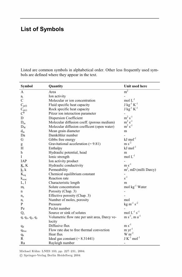
List of Symbols
Listed are common symbols in alphabetical order. Other less frequently used sym-
bols are defined where they appear in the text.
Symbol Quantity Unit used here
A Area m2
ai Ion activity -
C Molecular or ion concentration mol L-1
Cp(f) Fluid specific heat capacity J kg-1
K-1
Cp(r) Rock specific heat capacity J kg-1
K-1
Cφ
Pitzer ion interaction parameter -
D Dispersion Coefficient m2 s
-1
Dm Molecular diffusion coeff. (porous medium) m2 s
-1
DW Molecular diffusion coefficent (open water) m2 s
-1
dm Mean grain diameter m
Da Damköhler number -
G Gibbs free energy kJ mol-1
g Gravitational acceleration (= 9.81) m s-2
H Enthalpy kJ mol-1
h Hydraulic potential, head m
I Ionic strength mol L-1
IAP Ion activity product -
K, K Hydraulic conductivity m s-1
k, k Permeability m2, mD (milli Darcy)
Keq Chemical equilibrium constant -
kreac Reaction rate s-1
L, l Characteristic length m
mi Solute concentration mol kg-1
Water
n Porosity (Chap. 3) -
ne Effective porosity (Chap. 3) -
ni Number of moles, porosity mol
P Pressure kg m-1
s-2
Pe Peclet number -
Qs Source or sink of solutes mol L-1
s-1
q, qx, qy, qz Volumetric flow rate per unit area, Darcy ve-
locity
m s-1
, m a-1
qd Diffusive flux m s-1
qfree Flow rate due to free thermal convection m yr-1
qh Heat flux W m-2
R Ideal gas constant (= 8.31441) J K-1
mol-1
Ra Rayleigh number -
Michael Kuhn: LNES 103, pp. 227–231, 2004.c© Springer-Verlag Berlin Heidelberg 2004
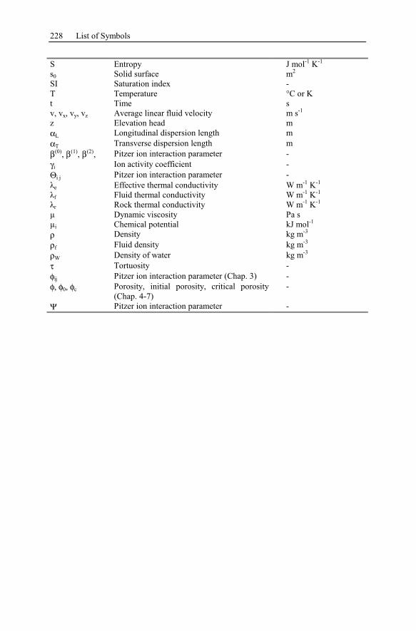
228 List of Symbols
S Entropy J mol-1
K-1
s0 Solid surface m2
SI Saturation index -
T Temperature °C or K
t Time s
v, vx, vy, vz Average linear fluid velocity m s-1
z Elevation head m
αLLongitudinal dispersion length m
αTTransverse dispersion length m
β(0), β(1)
, β(2), Pitzer ion interaction parameter -
γiIon activity coefficient -
Θi jPitzer ion interaction parameter -
e Effective thermal conductivity W m-1
K-1
f Fluid thermal conductivity W m-1
K-1
r Rock thermal conductivity W m-1
K-1
µ Dynamic viscosity Pa s
µi Chemical potential kJ mol-1
ρ Density kg m-3
ρfFluid density kg m
-3
ρWDensity of water kg m
-3
τ Tortuosity -
φijPitzer ion interaction parameter (Chap. 3) -
φ, φ0, φcPorosity, initial porosity, critical porosity
(Chap. 4-7)
-
Ψ Pitzer ion interaction parameter -
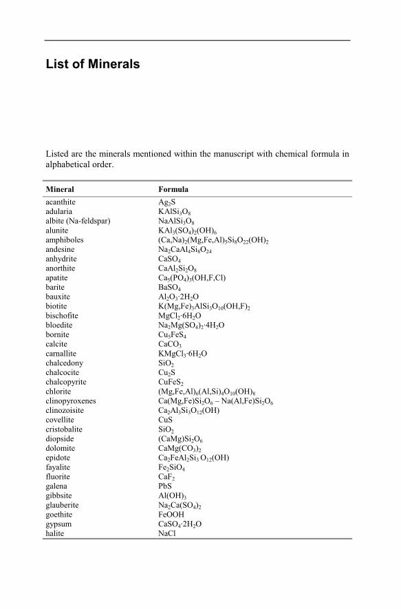
List of Minerals
Listed are the minerals mentioned within the manuscript with chemical formula in
alphabetical order.
Mineral Formula
acanthite Ag2S
adularia KAlSi3O8
albite (Na-feldspar) NaAlSi3O8
alunite KAl3(SO4)2(OH)6
amphiboles (Ca,Na)2(Mg,Fe,Al)5Si8O22(OH)2
andesine Na2CaAl4Si8O24
anhydrite CaSO4
anorthite CaAl2Si2O8
apatite Ca5(PO4)3(OH,F,Cl)
barite BaSO4
bauxite Al2O3·2H2O
biotite K(Mg,Fe)3AlSi3O10(OH,F)2
bischofite MgCl2·6H2O
bloedite Na2Mg(SO4)2·4H2O
bornite Cu5FeS4
calcite CaCO3
carnallite KMgCl3·6H2O
chalcedony SiO2
chalcocite Cu2S
chalcopyrite CuFeS2
chlorite (Mg,Fe,Al)6(Al,Si)4O10(OH)8
clinopyroxenes Ca(Mg,Fe)Si2O6 – Na(Al,Fe)Si2O6
clinozoisite Ca2Al3Si3O12(OH)
covellite CuS
cristobalite SiO2
diopside (CaMg)Si2O6
dolomite CaMg(CO3)2
epidote Ca2FeAl2Si3 O12(OH)
fayalite Fe2SiO4
fluorite CaF2
galena PbS
gibbsite Al(OH)3
glauberite Na2Ca(SO4)2
goethite FeOOH
gypsum CaSO4·2H2O
halite NaCl
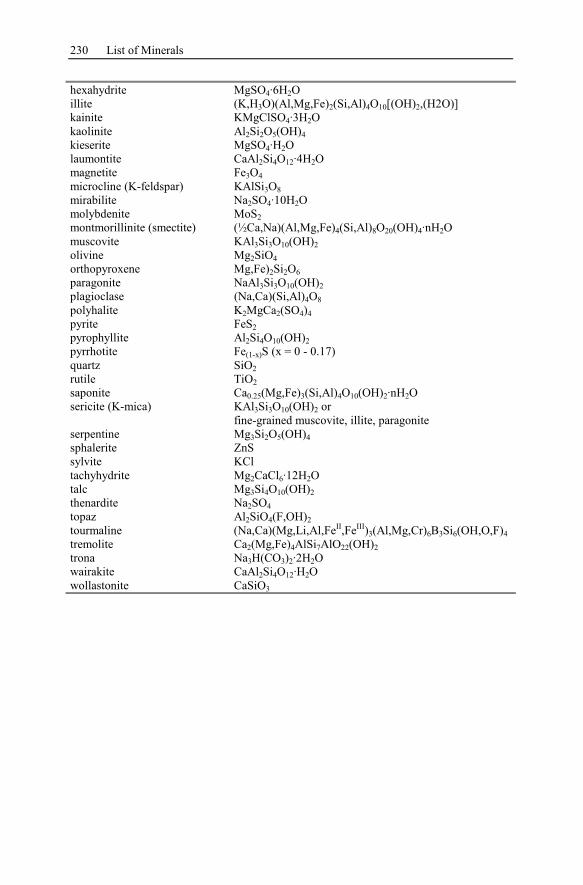
230 List of Minerals
hexahydrite MgSO4·6H2O
illite (K,H3O)(Al,Mg,Fe)2(Si,Al)4O10[(OH)2,(H2O)]
kainite KMgClSO4·3H2O
kaolinite Al2Si2O5(OH)4
kieserite MgSO4·H2O
laumontite CaAl2Si4O12·4H2O
magnetite Fe3O4
microcline (K-feldspar) KAlSi3O8
mirabilite Na2SO4·10H2O
molybdenite MoS2
montmorillinite (smectite) (½Ca,Na)(Al,Mg,Fe)4(Si,Al)8O20(OH)4·nH2O
muscovite KAl3Si3O10(OH)2
olivine Mg2SiO4
orthopyroxene Mg,Fe)2Si2O6
paragonite NaAl3Si3O10(OH)2
plagioclase (Na,Ca)(Si,Al)4O8
polyhalite K2MgCa2(SO4)4
pyrite FeS2
pyrophyllite Al2Si4O10(OH)2
pyrrhotite Fe(1-x)S (x = 0 - 0.17)
quartz SiO2
rutile TiO2
saponite Ca0.25(Mg,Fe)3(Si,Al)4O10(OH)2·nH2O
sericite (K-mica) KAl3Si3O10(OH)2 or
fine-grained muscovite, illite, paragonite
serpentine Mg3Si2O5(OH)4
sphalerite ZnS
sylvite KCl
tachyhydrite Mg2CaCl6·12H2O
talc Mg3Si4O10(OH)2
thenardite Na2SO4
topaz Al2SiO4(F,OH)2
tourmaline (Na,Ca)(Mg,Li,Al,FeII,Fe
III)3(Al,Mg,Cr)6B3Si6(OH,O,F)4
tremolite Ca2(Mg,Fe)4AlSi7AlO22(OH)2
trona Na3H(CO3)2·2H2O
wairakite CaAl2Si4O12·H2O
wollastonite CaSiO3
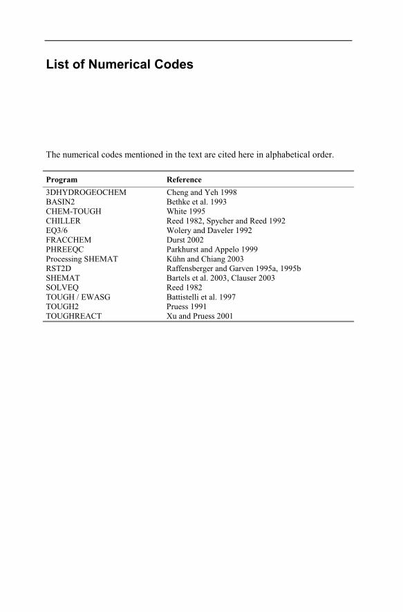
List of Numerical Codes
The numerical codes mentioned in the text are cited here in alphabetical order.
Program Reference
3DHYDROGEOCHEM Cheng and Yeh 1998
BASIN2 Bethke et al. 1993
CHEM-TOUGH White 1995
CHILLER Reed 1982, Spycher and Reed 1992
EQ3/6 Wolery and Daveler 1992
FRACCHEM Durst 2002
PHREEQC Parkhurst and Appelo 1999
Processing SHEMAT Kühn and Chiang 2003
RST2D Raffensberger and Garven 1995a, 1995b
SHEMAT Bartels et al. 2003, Clauser 2003
SOLVEQ Reed 1982
TOUGH / EWASG Battistelli et al. 1997
TOUGH2 Pruess 1991
TOUGHREACT Xu and Pruess 2001
Appendix
In the following section the compilation of geothermal waters from the literature
study (Chap. 2) is listed. These analyses meet the accuracy requirement of an ionic
strength in the range of ± 5 %. The compilation is based on the constituents Na, K,
Ca, Mg, Cl, SO4, and HCO3 / CO3 / CO2. Data for pH, temperature, and SiO2 are
listed if available.
The table is built up in a double paged listing. All samples are shown with their
reference, location, site, temperature, pH, sodium, potassium, calcium, magne-
sium, hydrogencarbonate, carbonate, carbon dioxide, and silica data. The samples
are alphabetically ordered by location.
• Reference: first author and year of the publication to be found in the references,
• Location: geothermal field location abbreviated with "continent / country / dis-
trict" following the ISO 3166 (International Standardisation Organisation,
Table A.1),
• Site: particular naming and kind of the drawing (e.g. well or spring),
• T: temperature of the sample as published,
• pH: measured pH of geothermal water if mentioned in the paper,
• unit: Unit of concentration of the particular water sample
• NA / K / CA / MG / CL / SO4 / HCO3 / CO3 / CO2 / SIO2: concentration of
sodium, potassium, calcium, magnesium, chloride, sulfate, hydrogencarbonate,
carbonate, carbon dioxide, and silica.
Table A.1. Used country codes from ISO 3166 (alphabetical by shorts)
Short Country Short Country Short Country
BG Bulgaria CA Canada CL Chile
CN China CO Colombia EG Egypt
SV El Salvador ET Ethopia DE Germany
GR Greece GT Guatemala HU Hungary
IS Iceland IN India ID Indonesia
IT Italy JP Japan MX Mexico
PA Panama PH Philippines LC Saint Lucia
SI Slovenia TH Thailand TR Turkey
GB United Kingdom US United States VN Vietnam
YU Yugoslavia
Michael Kuhn: LNES 103, pp. 233–261, 2004.c© Springer-Verlag Berlin Heidelberg 2004
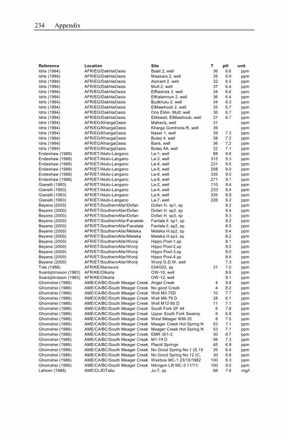
234 Appendix
Reference Location Site T pH unit
Idris (1994) AFR/EG/DakhlaOasis Balat 2, well 36 6.6 ppm
Idris (1994) AFR/EG/DakhlaOasis Maasara 2, well 35 6.9 ppm
Idris (1994) AFR/EG/DakhlaOasis Asmant 2, well 32 6.5 ppm
Idris (1994) AFR/EG/DakhlaOasis Mutt 2, well 37 6.4 ppm
Idris (1994) AFR/EG/DakhlaOasis ElRashda 3, well 34 6.6 ppm
Idris (1994) AFR/EG/DakhlaOasis ElKalamoun 2, well 36 6.4 ppm
Idris (1994) AFR/EG/DakhlaOasis Budkhulu 2, well 34 6.3 ppm
Idris (1994) AFR/EG/DakhlaOasis ElMawhoob 2, well 35 6.7 ppm
Idris (1994) AFR/EG/DakhlaOasis Ons ElAin, Mutt, well 30 6.7 ppm
Idris (1994) AFR/EG/DakhlaOasis ElAbeed, ElMawhoub, well 37 6.7 ppm
Idris (1994) AFR/EG/KhargaOasis Mahariq, well 31 ppm
Idris (1994) AFR/EG/KhargaOasis Kharga Gomhoria R, well 39 ppm
Idris (1994) AFR/EG/KhargaOasis Naser 1, well 39 7.3 ppm
Idris (1994) AFR/EG/KhargaOasis Bulaq 4, well 38 7.2 ppm
Idris (1994) AFR/EG/KhargaOasis Baris, well 36 7.2 ppm
Idris (1994) AFR/EG/KhargaOasis Bulaq 4A, well 32 7.1 ppm
Endeshaw (1988) AFR/ET/Aluto-Langano La-1, well 88 9.6 ppm
Endeshaw (1988) AFR/ET/Aluto-Langano La-3, well 315 9.3 ppm
Endeshaw (1988) AFR/ET/Aluto-Langano La-4, well 231 9.5 ppm
Endeshaw (1988) AFR/ET/Aluto-Langano La-5, well 208 9.0 ppm
Endeshaw (1988) AFR/ET/Aluto-Langano La-6, well 335 9.0 ppm
Endeshaw (1988) AFR/ET/Aluto-Langano La-8, well 271 9.1 ppm
Gianelli (1993) AFR/ET/Aluto-Langano La-2, well 110 9.4 ppm
Gianelli (1993) AFR/ET/Aluto-Langano La-4, well 233 8.4 ppm
Gianelli (1993) AFR/ET/Aluto-Langano La-6, well 335 6.9 ppm
Gianelli (1993) AFR/ET/Aluto-Langano La-7, well 226 8.2 ppm
Beyene (2000) AFR/ET/SouthernAfar/Dofan Dofan H. sp1, sp 8.2 ppm
Beyene (2000) AFR/ET/SouthernAfar/Dofan Dofan H. sp2, sp 8.4 ppm
Beyene (2000) AFR/ET/SouthernAfar/Dofan Dofan H. sp3, sp 8.3 ppm
Beyene (2000) AFR/ET/SouthernAfar/Fanatale Fantale ll. sp1, sp 8.2 ppm
Beyene (2000) AFR/ET/SouthernAfar/Fanatale Fantale ll. sp2, sp 8.5 ppm
Beyene (2000) AFR/ET/SouthernAfar/Meteka Meteka H.sp2, sp 8.4 ppm
Beyene (2000) AFR/ET/SouthernAfar/Meteka Meteka H.sp3, sp 8.2 ppm
Beyene (2000) AFR/ET/SouthernAfar/Wonji Hippo Pool-1,sp 8.1 ppm
Beyene (2000) AFR/ET/SouthernAfar/Wonji Hippo Pool-2,sp 8.0 ppm
Beyene (2000) AFR/ET/SouthernAfar/Wonji Hippo Pool-3,sp 8.0 ppm
Beyene (2000) AFR/ET/SouthernAfar/Wonji Hippo Pool-4,sp 8.4 ppm
Beyene (2000) AFR/ET/SouthernAfar/Wonji Wonji G.D.W, well 7.3 ppm
Tole (1988) AFR/KE/Narosura 034/002, sp 31 7.0 ppm
Svanbjörnsson (1983) AFR/KE/Olkaria OW-10, well 8.6 ppm
Svanbjörnsson (1983) AFR/KE/Olkaria OW-12, well 9.1 ppm
Ghomshei (1986) AME/CA/BC/South Meager Creek Angel Creek 4 9.6 ppm
Ghomshei (1986) AME/CA/BC/South Meager Creek No good Creek 4 8.2 ppm
Ghomshei (1986) AME/CA/BC/South Meager Creek Well M2-75D 10 7.7 ppm
Ghomshei (1986) AME/CA/BC/South Meager Creek Well M6-79 D 28 6.1 ppm
Ghomshei (1986) AME/CA/BC/South Meager Creek Well M12-80 D 11 7.1 ppm
Ghomshei (1986) AME/CA/BC/South Meager Creek South Fork SF 44 6 7.6 ppm
Ghomshei (1986) AME/CA/BC/South Meager Creek Upper South Fork Swamp 6 6.8 ppm
Ghomshei (1986) AME/CA/BC/South Meager Creek West Meager WM-35 8 7.0 ppm
Ghomshei (1986) AME/CA/BC/South Meager Creek Meager Creek Hot Spring N 53 7.1 ppm
Ghomshei (1986) AME/CA/BC/South Meager Creek Meager Creek Hot Spring N 53 7.1 ppm
Ghomshei (1986) AME/CA/BC/South Meager Creek EMR 301-2 30 6.7 ppm
Ghomshei (1986) AME/CA/BC/South Meager Creek M1-74 D 56 7.3 ppm
Ghomshei (1986) AME/CA/BC/South Meager Creek Placid Springs 45 6.9 ppm
Ghomshei (1986) AME/CA/BC/South Meager Creek No Good Spring No.1 (S,19 35 6.4 ppm
Ghomshei (1986) AME/CA/BC/South Meager Creek No Good Spring No.12 (C, 30 6.8 ppm
Ghomshei (1986) AME/CA/BC/South Meager Creek Weirbox MC-1 23/10/1982 100 8.3 ppm
Ghomshei (1986) AME/CA/BC/South Meager Creek Nitrogen Lift MC-3 11/11/ 100 9.0 ppm
Lahsen (1988) AME/CL/ElTatio Ju-7, sp 66 7.6 mg/l
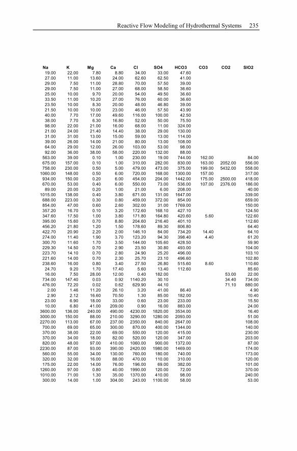
Reactive Flow Modeling of Hydrothermal Systems 235
Na K Mg Ca Cl SO4 HCO3 CO3 CO2 SIO2
19.00 22.00 7.80 8.80 34.00 33.00 47.60
27.00 11.00 13.60 24.00 62.60 62.50 41.00
29.00 7.50 11.00 28.80 70.00 57.50 39.00
29.00 7.50 11.00 27.00 68.00 58.50 36.60
25.00 10.00 9.70 20.00 54.00 49.50 36.60
33.50 11.00 10.20 27.00 76.00 60.00 36.60
23.50 10.00 8.30 20.00 48.00 46.80 39.00
21.50 10.00 10.00 23.00 46.00 57.50 43.90
40.00 7.70 17.00 49.60 116.00 100.00 42.50
38.00 7.70 6.30 16.80 52.00 50.00 75.50
98.00 22.00 21.00 16.00 68.00 11.00 324.00
21.00 24.00 21.40 14.40 38.00 29.00 130.00
31.00 31.00 13.00 15.00 59.00 13.00 114.00
39.00 26.00 14.00 21.00 80.00 13.00 108.00
64.00 29.00 12.00 26.00 103.00 53.00 98.00
92.00 36.00 38.00 58.00 220.00 132.00 88.00
563.00 39.00 0.10 1.00 230.00 19.00 744.00 162.00 84.00
675.00 157.00 0.10 1.00 310.00 282.00 830.00 163.00 2052.00 556.00
758.00 230.00 0.50 5.00 479.00 473.00 375.00 199.00 5432.00 558.00
1060.00 148.00 0.50 6.00 720.00 168.00 1300.00 157.00 317.00
934.00 150.00 0.20 6.00 454.00 204.00 1442.00 175.00 2500.00 418.00
670.00 53.00 0.40 6.00 550.00 73.00 536.00 107.00 2376.00 186.00
89.00 20.00 0.20 1.00 21.00 6.00 208.00 40.00
1015.00 138.00 0.40 3.80 671.00 131.00 1647.00 339.00
688.00 223.00 0.30 0.80 459.00 372.00 854.00 659.00
854.00 47.00 0.60 2.60 302.00 31.00 1769.00 150.00
357.20 16.70 0.10 3.20 172.60 168.10 427.10 124.50
347.60 17.50 1.00 3.80 171.80 164.80 420.60 5.60 122.60
395.00 15.60 0.70 8.80 204.60 216.40 401.10 112.60
456.20 21.80 1.20 1.50 178.60 89.30 806.80 64.40
422.70 20.90 2.20 2.00 146.10 84.00 734.20 14.40 64.10
274.00 11.40 1.90 3.70 123.20 94.30 398.40 4.40 61.20
300.70 11.60 1.70 3.50 144.00 105.60 428.50 59.90
229.30 14.50 0.70 2.90 23.50 30.80 493.00 104.00
223.70 14.10 0.70 2.80 24.90 25.20 496.00 103.10
221.60 14.00 0.70 2.30 25.70 23.10 496.60 102.80
238.60 16.00 0.80 3.40 27.50 26.80 515.60 8.60 110.60
24.70 9.20 1.70 17.40 5.60 13.40 112.60 85.60
16.00 7.50 28.00 12.00 0.40 182.00 53.00 22.00
734.00 147.40 0.03 0.92 1140.20 30.10 34.40 734.00
476.00 72.20 0.02 0.62 629.90 44.10 71.10 880.00
2.00 1.46 11.20 26.10 3.20 41.00 86.40 4.90
2.90 2.12 16.60 70.50 1.30 85.00 182.00 10.40
23.00 6.90 18.00 33.00 0.60 23.00 233.00 15.50
10.00 6.80 41.00 209.00 0.90 16.00 883.00 24.00
3600.00 136.00 240.00 490.00 4230.00 1820.00 3534.00 16.40
3000.00 150.00 88.00 210.00 3290.00 1280.00 2093.00 51.00
2270.00 113.00 67.00 237.00 2350.00 840.00 2647.00 108.00
700.00 69.00 65.00 300.00 870.00 400.00 1344.00 140.00
370.00 38.00 22.00 69.00 550.00 120.00 415.00 230.00
370.00 34.00 18.00 82.00 520.00 120.00 347.00 203.00
820.00 48.00 97.00 410.00 1060.00 900.00 1372.00 87.00
2230.00 87.00 93.00 390.00 2420.00 1980.00 1469.00 174.00
560.00 55.00 34.00 130.00 760.00 180.00 740.00 173.00
320.00 32.00 16.00 88.00 470.00 110.00 310.00 120.00
175.00 22.00 14.00 76.00 196.00 69.00 382.00 101.00
1260.00 97.00 0.80 40.00 1990.00 120.00 72.00 370.00
1010.00 71.00 1.30 35.00 1370.00 410.00 98.00 240.00
300.00 14.00 1.00 304.00 243.00 1100.00 58.00 53.00
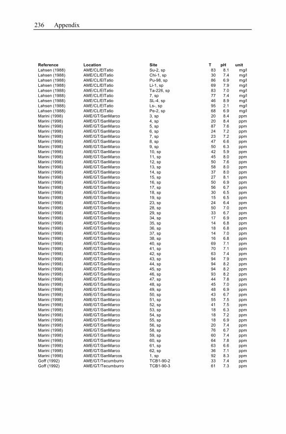
236 Appendix
Reference Location Site T pH unit
Lahsen (1988) AME/CL/ElTatio Su-2, sp 83 8.1 mg/l
Lahsen (1988) AME/CL/ElTatio Chi-1, sp 30 7.4 mg/l
Lahsen (1988) AME/CL/ElTatio Pu-98, sp 86 6.9 mg/l
Lahsen (1988) AME/CL/ElTatio Li-1, sp 69 7.9 mg/l
Lahsen (1988) AME/CL/ElTatio Ta-226, sp 83 7.0 mg/l
Lahsen (1988) AME/CL/ElTatio 7, sp 77 7.4 mg/l
Lahsen (1988) AME/CL/ElTatio SL-4, sp 46 8.9 mg/l
Lahsen (1988) AME/CL/ElTatio Ls-, sp 95 2.1 mg/l
Lahsen (1988) AME/CL/ElTatio Pe-2, sp 68 6.9 mg/l
Marini (1998) AME/GT/SanMarco 3, sp 20 8.4 ppm
Marini (1998) AME/GT/SanMarco 4, sp 20 8.4 ppm
Marini (1998) AME/GT/SanMarco 5, sp 87 7.6 ppm
Marini (1998) AME/GT/SanMarco 6, sp 24 7.2 ppm
Marini (1998) AME/GT/SanMarco 7, sp 23 7.2 ppm
Marini (1998) AME/GT/SanMarco 8, sp 47 6.6 ppm
Marini (1998) AME/GT/SanMarco 9, sp 50 6.3 ppm
Marini (1998) AME/GT/SanMarco 10, sp 42 5.9 ppm
Marini (1998) AME/GT/SanMarco 11, sp 45 8.0 ppm
Marini (1998) AME/GT/SanMarco 12, sp 50 7.6 ppm
Marini (1998) AME/GT/SanMarco 13, sp 58 8.0 ppm
Marini (1998) AME/GT/SanMarco 14, sp 37 8.0 ppm
Marini (1998) AME/GT/SanMarco 15, sp 27 8.1 ppm
Marini (1998) AME/GT/SanMarco 16, sp 50 6.9 ppm
Marini (1998) AME/GT/SanMarco 17, sp 56 6.7 ppm
Marini (1998) AME/GT/SanMarco 18, sp 30 6.5 ppm
Marini (1998) AME/GT/SanMarco 19, sp 15 6.5 ppm
Marini (1998) AME/GT/SanMarco 23, sp 24 6.4 ppm
Marini (1998) AME/GT/SanMarco 28, sp 50 7.0 ppm
Marini (1998) AME/GT/SanMarco 29, sp 33 6.7 ppm
Marini (1998) AME/GT/SanMarco 34, sp 17 6.9 ppm
Marini (1998) AME/GT/SanMarco 35, sp 14 6.8 ppm
Marini (1998) AME/GT/SanMarco 36, sp 18 6.8 ppm
Marini (1998) AME/GT/SanMarco 37, sp 14 7.0 ppm
Marini (1998) AME/GT/SanMarco 38, sp 16 6.8 ppm
Marini (1998) AME/GT/SanMarco 40, sp 69 7.1 ppm
Marini (1998) AME/GT/SanMarco 41, sp 70 7.1 ppm
Marini (1998) AME/GT/SanMarco 42, sp 63 7.4 ppm
Marini (1998) AME/GT/SanMarco 43, sp 94 7.9 ppm
Marini (1998) AME/GT/SanMarco 44, sp 94 8.2 ppm
Marini (1998) AME/GT/SanMarco 45, sp 94 8.2 ppm
Marini (1998) AME/GT/SanMarco 46, sp 93 8.2 ppm
Marini (1998) AME/GT/SanMarco 47, sp 44 7.8 ppm
Marini (1998) AME/GT/SanMarco 48, sp 45 7.0 ppm
Marini (1998) AME/GT/SanMarco 49, sp 48 6.9 ppm
Marini (1998) AME/GT/SanMarco 50, sp 43 6.7 ppm
Marini (1998) AME/GT/SanMarco 51, sp 55 7.5 ppm
Marini (1998) AME/GT/SanMarco 52, sp 41 7.5 ppm
Marini (1998) AME/GT/SanMarco 53, sp 18 6.3 ppm
Marini (1998) AME/GT/SanMarco 54, sp 18 7.2 ppm
Marini (1998) AME/GT/SanMarco 55, sp 18 6.9 ppm
Marini (1998) AME/GT/SanMarco 56, sp 20 7.4 ppm
Marini (1998) AME/GT/SanMarco 58, sp 76 6.7 ppm
Marini (1998) AME/GT/SanMarco 59, sp 60 7.4 ppm
Marini (1998) AME/GT/SanMarco 60, sp 64 7.8 ppm
Marini (1998) AME/GT/SanMarco 61, sp 63 6.6 ppm
Marini (1998) AME/GT/SanMarco 62, sp 36 7.1 ppm
Marini (1998) AME/GT/SanMarcos 1, sp 92 8.3 ppm
Goff (1992) AME/GT/Tecumburro TCB1-90-2 33 7.4 ppm
Goff (1992) AME/GT/Tecumburro TCB1-90-3 61 7.3 ppm
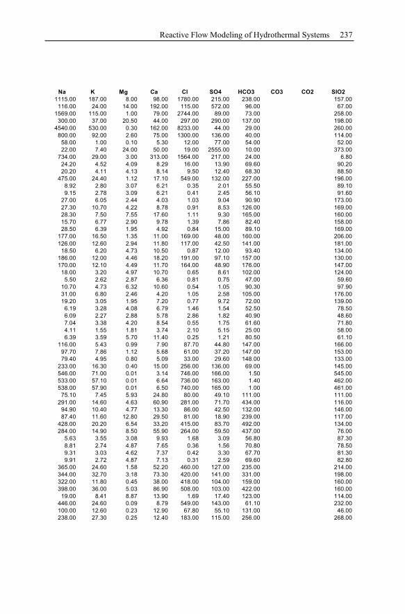
Reactive Flow Modeling of Hydrothermal Systems 237
Na K Mg Ca Cl SO4 HCO3 CO3 CO2 SIO2
1115.00 187.00 8.00 98.00 1780.00 215.00 238.00 157.00
116.00 24.00 14.00 192.00 115.00 572.00 96.00 67.00
1569.00 115.00 1.00 79.00 2744.00 89.00 73.00 258.00
300.00 37.00 20.50 44.00 297.00 290.00 137.00 198.00
4540.00 530.00 0.30 162.00 8233.00 44.00 29.00 260.00
800.00 92.00 2.60 75.00 1300.00 136.00 40.00 114.00
58.00 1.00 0.10 5.30 12.00 77.00 54.00 52.00
22.00 7.40 24.00 50.00 19.00 2555.00 10.00 373.00
734.00 29.00 3.00 313.00 1564.00 217.00 24.00 6.80
24.20 4.52 4.09 8.29 16.00 13.90 69.60 90.20
20.20 4.11 4.13 8.14 9.50 12.40 68.30 88.50
475.00 24.40 1.12 17.10 549.00 132.00 227.00 196.00
8.92 2.80 3.07 6.21 0.35 2.01 55.50 89.10
9.15 2.78 3.09 6.21 0.41 2.45 56.10 91.60
27.00 6.05 2.44 4.03 1.03 9.04 90.90 173.00
27.30 10.70 4.22 8.78 0.91 8.53 126.00 169.00
28.30 7.50 7.55 17.60 1.11 9.30 165.00 160.00
15.70 6.77 2.90 9.78 1.39 7.86 82.40 158.00
28.50 6.39 1.95 4.92 0.84 15.00 89.10 169.00
177.00 16.50 1.35 11.00 169.00 48.00 160.00 206.00
126.00 12.60 2.94 11.80 117.00 42.50 141.00 181.00
18.50 6.20 4.73 10.50 0.87 12.00 93.40 134.00
186.00 12.00 4.46 18.20 191.00 97.10 157.00 130.00
170.00 12.10 4.49 11.70 164.00 48.90 176.00 147.00
18.00 3.20 4.97 10.70 0.65 8.61 102.00 124.00
5.50 2.62 2.87 6.36 0.81 0.75 47.00 59.60
10.70 4.73 6.32 10.60 0.54 1.05 90.30 97.90
31.00 6.80 2.46 4.20 1.05 2.58 105.00 176.00
19.20 3.05 1.95 7.20 0.77 9.72 72.00 139.00
6.19 3.28 4.08 6.79 1.46 1.54 52.50 78.50
6.09 2.27 2.88 5.78 2.86 1.82 40.90 48.60
7.04 3.38 4.20 8.54 0.55 1.75 61.60 71.80
4.11 1.55 1.81 3.74 2.10 5.15 25.00 58.00
6.39 3.59 5.70 11.40 0.25 1.21 80.50 61.10
116.00 5.43 0.99 7.90 87.70 44.80 147.00 166.00
97.70 7.86 1.12 5.68 61.00 37.20 147.00 153.00
79.40 4.95 0.80 5.09 33.00 29.60 148.00 133.00
233.00 16.30 0.40 15.00 256.00 136.00 69.00 145.00
546.00 71.00 0.01 3.14 746.00 166.00 1.50 545.00
533.00 57.10 0.01 6.64 736.00 163.00 1.40 462.00
538.00 57.90 0.01 6.50 740.00 165.00 1.00 461.00
75.10 7.45 5.93 24.80 80.00 49.10 111.00 111.00
291.00 14.60 4.63 60.90 281.00 71.70 434.00 116.00
94.90 10.40 4.77 13.30 86.00 42.50 132.00 146.00
87.40 11.60 12.80 29.50 81.00 18.90 239.00 117.00
428.00 20.20 6.54 33.20 415.00 83.70 492.00 134.00
284.00 14.90 8.50 55.90 264.00 59.50 437.00 76.00
5.63 3.55 3.08 9.93 1.68 3.09 56.80 87.30
8.81 2.74 4.87 7.65 0.36 1.56 70.80 78.50
9.31 3.03 4.62 7.37 0.42 3.30 67.70 81.30
9.91 2.72 4.87 7.13 0.31 2.59 69.60 82.80
365.00 24.60 1.58 52.20 460.00 127.00 235.00 214.00
344.00 32.70 3.18 73.30 420.00 141.00 331.00 198.00
322.00 11.80 0.45 38.00 418.00 104.00 159.00 160.00
398.00 36.00 5.03 86.90 508.00 103.00 422.00 160.00
19.00 8.41 8.87 13.90 1.69 17.40 123.00 114.00
446.00 24.60 0.09 8.79 549.00 143.00 61.10 232.00
100.00 12.60 0.23 12.90 67.80 55.10 131.00 46.00
238.00 27.30 0.25 12.40 183.00 115.00 256.00 268.00
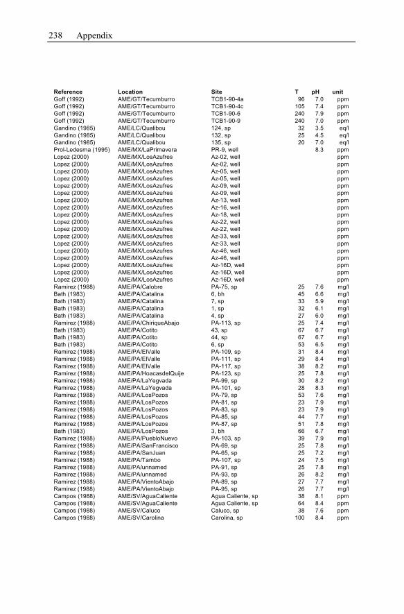
238 Appendix
Reference Location Site T pH unit
Goff (1992) AME/GT/Tecumburro TCB1-90-4a 96 7.0 ppm
Goff (1992) AME/GT/Tecumburro TCB1-90-4c 105 7.4 ppm
Goff (1992) AME/GT/Tecumburro TCB1-90-6 240 7.9 ppm
Goff (1992) AME/GT/Tecumburro TCB1-90-9 240 7.0 ppm
Gandino (1985) AME/LC/Qualibou 124, sp 32 3.5 eq/l
Gandino (1985) AME/LC/Qualibou 132, sp 25 4.5 eq/l
Gandino (1985) AME/LC/Qualibou 135, sp 20 7.0 eq/l
Prol-Ledesma (1995) AME/MX/LaPrimavera PR-9, well 8.3 ppm
Lopez (2000) AME/MX/LosAzufres Az-02, well ppm
Lopez (2000) AME/MX/LosAzufres Az-02, well ppm
Lopez (2000) AME/MX/LosAzufres Az-05, well ppm
Lopez (2000) AME/MX/LosAzufres Az-05, well ppm
Lopez (2000) AME/MX/LosAzufres Az-09, well ppm
Lopez (2000) AME/MX/LosAzufres Az-09, well ppm
Lopez (2000) AME/MX/LosAzufres Az-13, well ppm
Lopez (2000) AME/MX/LosAzufres Az-16, well ppm
Lopez (2000) AME/MX/LosAzufres Az-18, well ppm
Lopez (2000) AME/MX/LosAzufres Az-22, well ppm
Lopez (2000) AME/MX/LosAzufres Az-22, well ppm
Lopez (2000) AME/MX/LosAzufres Az-33, well ppm
Lopez (2000) AME/MX/LosAzufres Az-33, well ppm
Lopez (2000) AME/MX/LosAzufres Az-46, well ppm
Lopez (2000) AME/MX/LosAzufres Az-46, well ppm
Lopez (2000) AME/MX/LosAzufres Az-16D, well ppm
Lopez (2000) AME/MX/LosAzufres Az-16D, well ppm
Lopez (2000) AME/MX/LosAzufres Az-16D, well ppm
Ramirez (1988) AME/PA/Calobre PA-75, sp 25 7.6 mg/l
Bath (1983) AME/PA/Catalina 6, bh 45 6.6 mg/l
Bath (1983) AME/PA/Catalina 7, sp 33 5.9 mg/l
Bath (1983) AME/PA/Catalina 1, sp 32 6.1 mg/l
Bath (1983) AME/PA/Catalina 4, sp 27 6.0 mg/l
Ramirez (1988) AME/PA/ChiriqueAbajo PA-113, sp 25 7.4 mg/l
Bath (1983) AME/PA/Cotito 43, sp 67 6.7 mg/l
Bath (1983) AME/PA/Cotito 44, sp 67 6.7 mg/l
Bath (1983) AME/PA/Cotito 6, sp 53 6.5 mg/l
Ramirez (1988) AME/PA/ElValle PA-109, sp 31 8.4 mg/l
Ramirez (1988) AME/PA/ElValle PA-111, sp 29 8.4 mg/l
Ramirez (1988) AME/PA/ElValle PA-117, sp 38 8.2 mg/l
Ramirez (1988) AME/PA/HoacasdelQuije PA-123, sp 25 7.8 mg/l
Ramirez (1988) AME/PA/LaYegvada PA-99, sp 30 8.2 mg/l
Ramirez (1988) AME/PA/LaYegvada PA-101, sp 28 8.3 mg/l
Ramirez (1988) AME/PA/LosPozos PA-79, sp 53 7.6 mg/l
Ramirez (1988) AME/PA/LosPozos PA-81, sp 23 7.9 mg/l
Ramirez (1988) AME/PA/LosPozos PA-83, sp 23 7.9 mg/l
Ramirez (1988) AME/PA/LosPozos PA-85, sp 44 7.7 mg/l
Ramirez (1988) AME/PA/LosPozos PA-87, sp 51 7.8 mg/l
Bath (1983) AME/PA/LosPozos 3, bh 66 6.7 mg/l
Ramirez (1988) AME/PA/PuebloNuevo PA-103, sp 39 7.9 mg/l
Ramirez (1988) AME/PA/SanFrancisco PA-69, sp 25 7.8 mg/l
Ramirez (1988) AME/PA/SanJuan PA-65, sp 25 7.2 mg/l
Ramirez (1988) AME/PA/Tambo PA-107, sp 24 7.5 mg/l
Ramirez (1988) AME/PA/unnamed PA-91, sp 25 7.8 mg/l
Ramirez (1988) AME/PA/unnamed PA-93, sp 26 8.2 mg/l
Ramirez (1988) AME/PA/VientoAbajo PA-89, sp 27 7.7 mg/l
Ramirez (1988) AME/PA/VientoAbajo PA-95, sp 26 7.7 mg/l
Campos (1988) AME/SV/AguaCaliente Agua Caliente, sp 38 8.1 ppm
Campos (1988) AME/SV/AguaCaliente Agua Caliente, sp 64 8.4 ppm
Campos (1988) AME/SV/Caluco Caluco, sp 38 7.6 ppm
Campos (1988) AME/SV/Carolina Carolina, sp 100 8.4 ppm
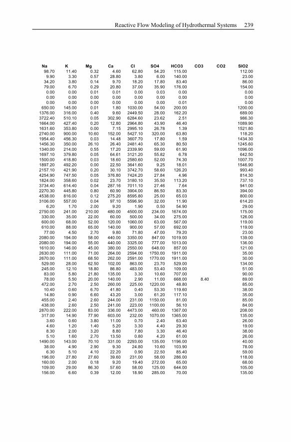
Reactive Flow Modeling of Hydrothermal Systems 239
Na K Mg Ca Cl SO4 HCO3 CO3 CO2 SIO2
98.70 11.40 0.32 4.60 62.80 54.20 115.00 112.00
9.90 3.30 0.57 28.80 3.80 6.00 140.00 23.00
34.20 3.80 0.14 9.70 18.20 17.80 83.40 86.00
79.00 6.70 0.29 20.80 37.00 35.90 176.00 154.00
0.00 0.00 0.01 0.01 0.00 0.03 0.00 0.00
0.00 0.00 0.00 0.00 0.00 0.00 0.00 0.00
0.00 0.00 0.00 0.00 0.00 0.00 0.01 0.00
650.00 145.00 0.01 1.80 1030.00 54.00 200.00 1200.00
1376.00 316.00 0.40 9.60 2449.50 28.00 162.20 689.00
3722.40 510.10 0.05 302.90 6284.60 23.62 2.51 986.30
1664.00 427.40 0.20 12.80 2964.80 43.90 46.40 1089.90
1631.60 353.80 0.00 7.15 2995.10 26.78 1.39 1521.80
2740.00 900.00 10.60 152.00 5427.10 320.00 63.80 118.20
1954.40 456.30 0.03 14.48 3607.70 17.80 1.59 1434.30
1456.30 350.00 26.10 26.40 2481.40 65.30 80.50 1245.60
1340.00 214.00 0.55 17.20 2339.90 59.00 61.90 1096.00
1697.10 379.80 0.05 64.61 3121.20 55.82 6.78 642.50
1500.00 418.80 0.03 18.60 2580.60 52.00 74.30 1007.70
1897.20 492.20 0.00 22.50 3641.60 9.25 18.01 1546.90
2157.10 421.90 0.20 30.10 3742.70 58.60 126.20 993.40
4254.90 747.50 0.05 376.80 7424.20 27.84 4.96 814.30
1824.00 358.60 0.02 23.70 3180.10 35.50 113.20 737.10
3734.40 614.40 0.04 287.16 7011.10 27.46 7.64 941.00
2270.30 445.80 0.80 60.90 3904.00 86.50 83.30 394.00
4538.00 816.00 0.12 275.20 8595.80 25.00 65.03 800.00
3106.00 557.00 0.04 97.10 5596.90 32.00 11.90 614.20
6.20 1.70 2.00 9.20 1.90 0.50 54.90 29.00
2750.00 241.00 210.00 480.00 4500.00 234.00 1674.00 175.00
330.00 35.00 22.00 60.00 500.00 34.00 275.00 126.00
600.00 68.00 52.00 120.00 1060.00 63.00 567.00 119.00
610.00 88.00 65.00 140.00 900.00 57.00 692.00 119.00
77.00 4.50 2.70 9.80 71.80 47.00 79.20 23.00
2080.00 194.00 58.00 440.00 3350.00 847.00 1019.00 139.00
2080.00 194.00 55.00 440.00 3325.00 777.00 1013.00 136.00
1610.00 146.00 45.00 380.00 2550.00 648.00 857.00 121.00
2630.00 111.00 71.00 264.00 2594.00 1750.00 1911.00 35.00
2670.00 111.00 68.50 262.00 2591.00 1770.00 1911.00 30.00
529.00 28.00 62.50 102.00 863.00 23.70 529.00 134.00
245.00 12.10 18.80 86.80 483.00 53.40 109.00 51.00
83.00 5.80 21.80 135.00 3.30 10.60 707.00 90.00
78.00 5.50 20.00 140.00 2.90 11.00 668.00 8.40 89.00
472.00 2.70 2.50 260.00 225.00 1220.00 48.80 85.00
10.40 0.60 6.70 41.80 0.40 53.30 119.60 38.00
14.80 0.90 6.60 43.20 3.00 61.20 117.10 35.00
455.00 2.40 2.60 244.00 231.00 1150.00 81.00 85.00
438.00 2.60 2.50 241.00 223.00 1100.00 56.10 84.00
2870.00 222.00 83.00 336.00 4473.00 460.00 1367.00 208.00
317.00 14.90 77.90 603.00 232.00 1070.00 1365.00 135.00
3.60 0.60 3.80 11.00 0.70 2.40 63.40 26.00
4.60 1.20 1.40 5.20 3.30 4.40 29.30 19.00
8.30 2.00 3.20 8.80 7.80 3.30 46.40 38.00
5.10 1.60 2.70 13.50 0.80 4.20 61.00 26.00
1490.00 143.00 70.10 331.00 2293.00 135.00 1196.00 40.00
38.00 4.90 2.90 9.30 24.80 10.60 103.90 78.00
6.30 5.10 4.10 22.20 0.90 22.50 85.40 59.00
196.00 27.80 27.60 39.60 231.00 58.00 286.00 118.00
160.00 2.00 0.18 9.20 19.40 272.00 65.00 68.00
109.00 29.00 86.30 57.60 58.00 125.00 644.00 105.00
156.00 6.60 0.39 12.00 18.90 285.00 70.00 135.00
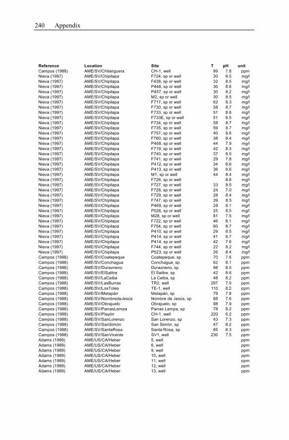
240 Appendix
Reference Location Site T pH unit
Campos (1988) AME/SV/Chilanguera CH-1, well 99 7.8 ppm
Nieva (1997) AME/SV/Chipilapa F724, sp or well 30 8.5 mg/l
Nieva (1997) AME/SV/Chipilapa F438, sp or well 32 8.5 mg/l
Nieva (1997) AME/SV/Chipilapa P448, sp or well 30 8.6 mg/l
Nieva (1997) AME/SV/Chipilapa P457, sp or well 30 8.2 mg/l
Nieva (1997) AME/SV/Chipilapa M2, sp or well 30 8.5 mg/l
Nieva (1997) AME/SV/Chipilapa F717, sp or well 62 8.3 mg/l
Nieva (1997) AME/SV/Chipilapa F730, sp or well 58 8.7 mg/l
Nieva (1997) AME/SV/Chipilapa F733, sp or well 51 8.6 mg/l
Nieva (1997) AME/SV/Chipilapa F733E, sp or well 51 8.5 mg/l
Nieva (1997) AME/SV/Chipilapa F734, sp or well 58 8.7 mg/l
Nieva (1997) AME/SV/Chipilapa F735, sp or well 59 8.7 mg/l
Nieva (1997) AME/SV/Chipilapa F757, sp or well 40 8.6 mg/l
Nieva (1997) AME/SV/Chipilapa F760, sp or well 38 8.4 mg/l
Nieva (1997) AME/SV/Chipilapa P468, sp or well 44 7.9 mg/l
Nieva (1997) AME/SV/Chipilapa F719, sp or well 42 8.3 mg/l
Nieva (1997) AME/SV/Chipilapa F740, sp or well 37 8.0 mg/l
Nieva (1997) AME/SV/Chipilapa F741, sp or well 29 7.8 mg/l
Nieva (1997) AME/SV/Chipilapa P412, sp or well 34 8.6 mg/l
Nieva (1997) AME/SV/Chipilapa P413, sp or well 36 8.6 mg/l
Nieva (1997) AME/SV/Chipilapa M1, sp or well 44 8.4 mg/l
Nieva (1997) AME/SV/Chipilapa F726, sp or well 8.6 mg/l
Nieva (1997) AME/SV/Chipilapa F727, sp or well 33 8.5 mg/l
Nieva (1997) AME/SV/Chipilapa F728, sp or well 24 7.0 mg/l
Nieva (1997) AME/SV/Chipilapa F729, sp or well 28 8.4 mg/l
Nieva (1997) AME/SV/Chipilapa F747, sp or well 39 8.5 mg/l
Nieva (1997) AME/SV/Chipilapa P469, sp or well 28 8.1 mg/l
Nieva (1997) AME/SV/Chipilapa P526, sp or well 25 8.5 mg/l
Nieva (1997) AME/SV/Chipilapa M28, sp or well 81 7.5 mg/l
Nieva (1997) AME/SV/Chipilapa F722, sp or well 46 8.1 mg/l
Nieva (1997) AME/SV/Chipilapa F754, sp or well 60 8.7 mg/l
Nieva (1997) AME/SV/Chipilapa P410, sp or well 29 8.5 mg/l
Nieva (1997) AME/SV/Chipilapa P414, sp or well 41 8.7 mg/l
Nieva (1997) AME/SV/Chipilapa P414, sp or well 42 7.6 mg/l
Nieva (1997) AME/SV/Chipilapa F744, sp or well 22 8.2 mg/l
Nieva (1997) AME/SV/Chipilapa P523, sp or well 26 8.4 mg/l
Campos (1988) AME/SV/Coatepeque Coatepeque, sp 70 7.6 ppm
Campos (1988) AME/SV/Conchagua Conchagua, sp 62 8.1 ppm
Campos (1988) AME/SV/Durazneno Durazneno, sp 98 8.0 ppm
Campos (1988) AME/SV/ElSalitre El Salitre, sp 42 8.6 ppm
Campos (1988) AME/SV/LaCeiba La Ceiba, sp 48 8.2 ppm
Campos (1988) AME/SV/LasBurras TR2, well 297 7.0 ppm
Campos (1988) AME/SV/LosToles TE-1, well 110 8.2 ppm
Campos (1988) AME/SV/Metapán Metapán, sp 79 7.8 ppm
Campos (1988) AME/SV/NombredeJesús Nombre de Jesús, sp 88 7.6 ppm
Campos (1988) AME/SV/Obrajuelo Obrajuelo, sp 98 7.9 ppm
Campos (1988) AME/SV/ParrasLempa Parras Lempa, sp 78 8.2 ppm
Campos (1988) AME/SV/Playón CH-1, well 220 6.2 ppm
Campos (1988) AME/SV/SanLorenzo San Lorenzo, sp 43 7.3 ppm
Campos (1988) AME/SV/SanSimón San Simón, sp 47 8.2 ppm
Campos (1988) AME/SV/SantaRosa Santa Rosa, sp 85 8.3 ppm
Campos (1988) AME/SV/SanVicente SV1, well 230 7.5 ppm
Adams (1989) AME/US/CA/Heber 5, well ppm
Adams (1989) AME/US/CA/Heber 6, well ppm
Adams (1989) AME/US/CA/Heber 9, well ppm
Adams (1989) AME/US/CA/Heber 10, well ppm
Adams (1989) AME/US/CA/Heber 11, well ppm
Adams (1989) AME/US/CA/Heber 12, well ppm
Adams (1989) AME/US/CA/Heber 13, well ppm
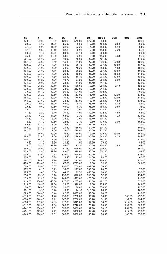
Reactive Flow Modeling of Hydrothermal Systems 241
Na K Mg Ca Cl SO4 HCO3 CO3 CO2 SIO2
470.00 22.00 0.32 130.00 579.00 477.00 40.30 120.00
22.60 5.60 11.70 25.00 6.50 12.50 156.00 2.50 90.00
37.00 6.90 11.00 22.00 23.20 14.00 150.00 5.40 94.00
37.20 9.60 13.10 28.80 26.90 12.00 183.00 7.20 85.00
38.20 7.40 13.60 29.00 27.70 12.00 200.00 89.00
35.40 6.20 10.00 24.60 23.90 13.30 156.00 3.60 96.00
201.00 23.00 3.60 13.90 75.00 29.90 461.00 143.00
187.00 23.60 3.50 15.10 81.80 27.90 394.00 22.80 156.00
128.00 20.80 7.00 34.00 80.70 30.40 337.00 10.80 137.00
132.00 21.00 7.20 34.00 78.20 29.70 358.00 4.80 152.00
164.00 23.00 4.70 23.40 80.20 29.30 387.00 10.80 150.00
175.00 22.80 4.20 20.40 86.90 28.70 376.00 15.60 143.00
109.00 17.50 4.60 22.40 46.70 26.00 265.00 13.80 128.00
100.00 15.20 4.60 18.70 37.20 22.20 256.00 6.00 128.00
174.00 20.00 6.00 23.80 61.80 25.40 447.00 132.00
154.00 25.20 12.10 29.80 185.00 17.80 254.00 2.40 128.00
229.00 39.00 10.30 28.00 342.00 19.90 244.00 133.00
70.00 15.70 12.80 26.80 104.00 10.70 162.00 96.00
139.00 25.20 12.60 36.80 183.00 16.40 220.00 12.00 133.00
154.00 24.40 10.00 30.40 170.00 9.50 232.00 12.00 118.00
148.00 23.60 10.60 28.40 187.00 17.10 265.00 4.80 136.00
29.90 9.50 11.20 53.00 0.40 95.40 158.00 6.10 81.00
29.30 9.60 10.80 49.00 0.30 98.30 153.00 3.60 76.00
12.00 2.70 8.30 36.40 3.50 33.40 133.00 64.00
11.50 2.20 8.40 39.50 4.00 40.60 132.00 1.80 64.00
23.40 6.20 14.20 64.00 2.30 138.00 168.00 1.20 121.00
15.10 4.50 8.20 28.20 2.00 48.40 101.00 87.00
12.50 4.10 10.80 22.60 2.70 2.60 135.00 3.00 102.00
49.80 17.80 5.90 24.60 2.60 126.00 85.00 219.00
165.00 23.40 6.50 21.40 136.00 21.40 301.00 146.00
167.00 22.20 7.00 15.00 118.00 22.00 331.00 146.00
71.50 16.60 16.00 36.40 140.00 12.70 139.00 15.00 101.00
166.00 23.60 7.00 22.40 149.00 20.90 248.00 4.20 144.00
164.00 24.30 7.80 22.80 152.00 20.50 297.00 139.00
10.20 3.30 3.90 21.20 1.90 27.50 76.00 54.00
25.00 24.40 31.50 85.00 83.10 30.90 308.00 1.80 96.00
286.00 38.00 55.50 47.40 476.00 130.00 303.00 107.00
130.00 8.50 27.50 48.00 210.00 52.00 201.00 86.70
875.00 23.40 0.17 218.00 1539.00 186.00 21.40 114.00
106.00 1.00 0.25 2.40 13.40 144.00 63.70 60.00
197.00 28.40 9.90 24.40 242.00 23.50 289.00 153.00
3750.00 835.00 0.43 67.00 6777.00 13.00 22.00 1001.00
560.00 15.80 0.07 116.00 709.00 482.00 38.80
272.00 6.10 0.23 34.00 183.00 396.00 90.70 77.00
175.00 9.40 8.00 44.90 22.70 456.00 88.00 156.00
650.00 19.50 0.10 150.00 1090.00 240.00 52.00 124.00
420.00 12.80 0.10 148.00 572.00 470.00 34.00 110.00
2410.00 186.00 48.00 137.00 4237.00 51.80 122.20 352.00
216.00 40.50 12.60 29.50 320.00 18.00 225.00 141.00
80.00 24.00 36.00 51.00 98.00 61.00 330.00 157.00
161.00 5.30 3.90 13.90 24.10 313.00 95.00 100.00
1620.00 240.00 0.40 82.00 2827.00 59.00 63.20 419.00
4019.00 333.00 1.76 750.00 7758.00 65.90 30.60 186.00 237.00
4034.00 340.00 2.12 747.00 7738.00 63.20 31.60 197.00 224.00
4060.00 332.00 2.05 717.00 7815.00 64.00 30.20 217.00 243.00
4012.00 342.00 1.96 686.00 7746.00 73.70 30.40 207.00 230.00
4242.00 354.00 2.81 655.00 7835.00 62.90 30.10 251.00 221.00
4261.00 349.00 2.42 736.00 7866.00 64.40 30.40 212.00 232.00
4140.00 324.00 2.31 565.00 7625.00 59.70 30.00 189.00 275.00
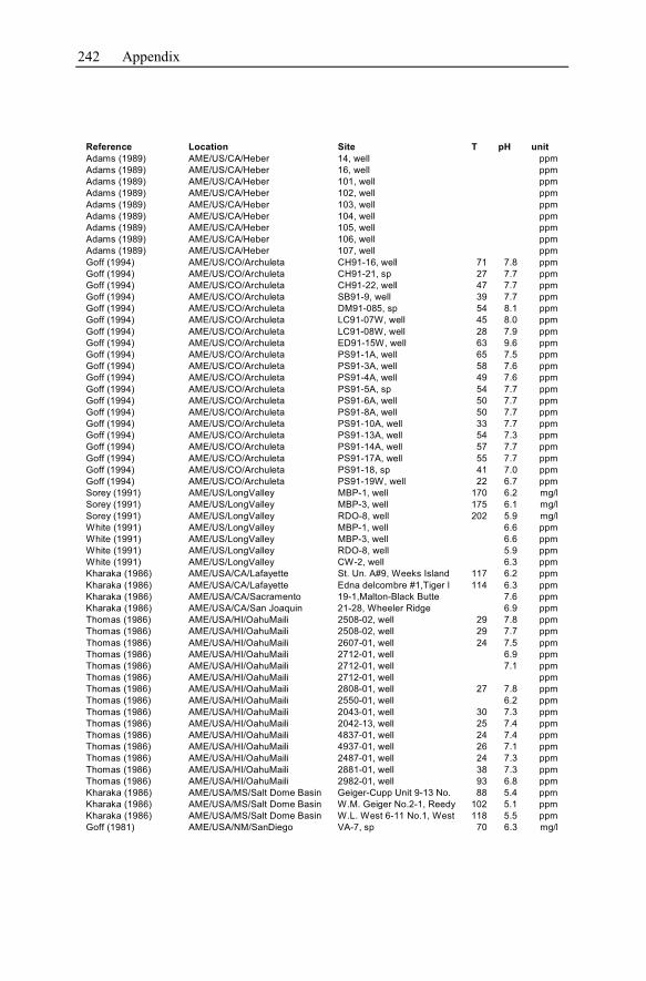
242 Appendix
Reference Location Site T pH unit
Adams (1989) AME/US/CA/Heber 14, well ppm
Adams (1989) AME/US/CA/Heber 16, well ppm
Adams (1989) AME/US/CA/Heber 101, well ppm
Adams (1989) AME/US/CA/Heber 102, well ppm
Adams (1989) AME/US/CA/Heber 103, well ppm
Adams (1989) AME/US/CA/Heber 104, well ppm
Adams (1989) AME/US/CA/Heber 105, well ppm
Adams (1989) AME/US/CA/Heber 106, well ppm
Adams (1989) AME/US/CA/Heber 107, well ppm
Goff (1994) AME/US/CO/Archuleta CH91-16, well 71 7.8 ppm
Goff (1994) AME/US/CO/Archuleta CH91-21, sp 27 7.7 ppm
Goff (1994) AME/US/CO/Archuleta CH91-22, well 47 7.7 ppm
Goff (1994) AME/US/CO/Archuleta SB91-9, well 39 7.7 ppm
Goff (1994) AME/US/CO/Archuleta DM91-085, sp 54 8.1 ppm
Goff (1994) AME/US/CO/Archuleta LC91-07W, well 45 8.0 ppm
Goff (1994) AME/US/CO/Archuleta LC91-08W, well 28 7.9 ppm
Goff (1994) AME/US/CO/Archuleta ED91-15W, well 63 9.6 ppm
Goff (1994) AME/US/CO/Archuleta PS91-1A, well 65 7.5 ppm
Goff (1994) AME/US/CO/Archuleta PS91-3A, well 58 7.6 ppm
Goff (1994) AME/US/CO/Archuleta PS91-4A, well 49 7.6 ppm
Goff (1994) AME/US/CO/Archuleta PS91-5A, sp 54 7.7 ppm
Goff (1994) AME/US/CO/Archuleta PS91-6A, well 50 7.7 ppm
Goff (1994) AME/US/CO/Archuleta PS91-8A, well 50 7.7 ppm
Goff (1994) AME/US/CO/Archuleta PS91-10A, well 33 7.7 ppm
Goff (1994) AME/US/CO/Archuleta PS91-13A, well 54 7.3 ppm
Goff (1994) AME/US/CO/Archuleta PS91-14A, well 57 7.7 ppm
Goff (1994) AME/US/CO/Archuleta PS91-17A, well 55 7.7 ppm
Goff (1994) AME/US/CO/Archuleta PS91-18, sp 41 7.0 ppm
Goff (1994) AME/US/CO/Archuleta PS91-19W, well 22 6.7 ppm
Sorey (1991) AME/US/LongValley MBP-1, well 170 6.2 mg/l
Sorey (1991) AME/US/LongValley MBP-3, well 175 6.1 mg/l
Sorey (1991) AME/US/LongValley RDO-8, well 202 5.9 mg/l
White (1991) AME/US/LongValley MBP-1, well 6.6 ppm
White (1991) AME/US/LongValley MBP-3, well 6.6 ppm
White (1991) AME/US/LongValley RDO-8, well 5.9 ppm
White (1991) AME/US/LongValley CW-2, well 6.3 ppm
Kharaka (1986) AME/USA/CA/Lafayette St. Un. A#9, Weeks Island 117 6.2 ppm
Kharaka (1986) AME/USA/CA/Lafayette Edna delcombre #1,Tiger l 114 6.3 ppm
Kharaka (1986) AME/USA/CA/Sacramento 19-1,Malton-Black Butte 7.6 ppm
Kharaka (1986) AME/USA/CA/San Joaquin 21-28, Wheeler Ridge 6.9 ppm
Thomas (1986) AME/USA/HI/OahuMaili 2508-02, well 29 7.8 ppm
Thomas (1986) AME/USA/HI/OahuMaili 2508-02, well 29 7.7 ppm
Thomas (1986) AME/USA/HI/OahuMaili 2607-01, well 24 7.5 ppm
Thomas (1986) AME/USA/HI/OahuMaili 2712-01, well 6.9 ppm
Thomas (1986) AME/USA/HI/OahuMaili 2712-01, well 7.1 ppm
Thomas (1986) AME/USA/HI/OahuMaili 2712-01, well ppm
Thomas (1986) AME/USA/HI/OahuMaili 2808-01, well 27 7.8 ppm
Thomas (1986) AME/USA/HI/OahuMaili 2550-01, well 6.2 ppm
Thomas (1986) AME/USA/HI/OahuMaili 2043-01, well 30 7.3 ppm
Thomas (1986) AME/USA/HI/OahuMaili 2042-13, well 25 7.4 ppm
Thomas (1986) AME/USA/HI/OahuMaili 4837-01, well 24 7.4 ppm
Thomas (1986) AME/USA/HI/OahuMaili 4937-01, well 26 7.1 ppm
Thomas (1986) AME/USA/HI/OahuMaili 2487-01, well 24 7.3 ppm
Thomas (1986) AME/USA/HI/OahuMaili 2881-01, well 38 7.3 ppm
Thomas (1986) AME/USA/HI/OahuMaili 2982-01, well 93 6.8 ppm
Kharaka (1986) AME/USA/MS/Salt Dome Basin Geiger-Cupp Unit 9-13 No. 88 5.4 ppm
Kharaka (1986) AME/USA/MS/Salt Dome Basin W.M. Geiger No.2-1, Reedy 102 5.1 ppm
Kharaka (1986) AME/USA/MS/Salt Dome Basin W.L. West 6-11 No.1, West 118 5.5 ppm
Goff (1981) AME/USA/NM/SanDiego VA-7, sp 70 6.3 mg/l
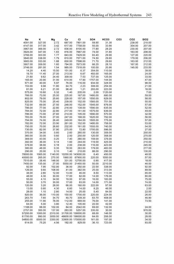
Reactive Flow Modeling of Hydrothermal Systems 243
Na K Mg Ca Cl SO4 HCO3 CO3 CO2 SIO2
4091.00 327.00 2.72 687.00 7801.00 59.90 31.30 238.00 210.00
4147.00 317.00 3.42 617.00 7758.00 55.00 33.90 304.00 207.00
3967.00 366.00 2.72 836.00 8105.00 77.80 28.20 230.00 207.00
3925.00 347.00 1.83 816.00 7667.00 74.00 31.60 163.00 208.00
3766.00 303.00 1.77 843.00 7429.00 83.40 29.90 127.00 220.00
3840.00 338.00 1.79 810.00 7571.00 74.50 29.60 179.00 206.00
3683.00 333.00 1.88 830.00 7598.00 71.70 29.60 163.00 212.00
3907.00 359.00 1.60 794.00 7673.00 66.20 28.10 167.00 212.00
3746.00 281.00 1.54 985.00 7318.00 100.00 20.90 145.00 233.00
14.20 4.40 15.50 151.00 6.37 354.00 110.00 39.00
19.70 11.40 27.00 213.00 6.67 493.00 165.00 24.00
21.60 9.62 24.40 309.00 7.53 737.00 125.00 33.00
165.00 20.90 31.00 614.00 17.90 1757.00 144.00 47.00
571.00 40.00 5.97 76.00 116.00 934.00 328.00 98.00
153.00 9.98 11.80 64.70 2.23 308.00 254.00 21.00
81.00 6.21 21.00 98.40 1.21 293.00 223.00 16.00
575.00 10.60 0.32 1.40 235.00 2.00 1120.00 7.00
766.00 73.00 25.00 225.00 167.00 1480.00 680.00 59.00
802.00 79.00 25.60 228.00 157.00 1550.00 629.00 58.00
825.00 75.00 25.40 239.00 152.00 1560.00 751.00 55.00
732.00 69.00 27.50 248.00 152.00 1545.00 676.00 57.00
786.00 77.00 22.80 216.00 139.00 1590.00 635.00 52.00
784.00 72.00 22.80 217.00 141.00 1575.00 639.00 49.00
786.00 73.00 27.60 214.00 105.00 1690.00 570.00 32.00
783.00 76.00 27.00 247.00 168.00 1620.00 792.00 56.00
794.00 74.00 26.40 249.00 164.00 1505.00 775.00 57.00
782.00 72.00 23.90 261.00 152.00 1495.00 758.00 53.00
750.00 70.00 26.60 232.00 161.00 1555.00 740.00 54.00
730.00 82.00 37.90 275.00 72.80 1700.00 596.00 27.00
370.00 34.00 0.60 2.60 260.00 130.00 359.00 250.00
360.00 33.00 0.60 2.50 250.00 120.00 358.00 270.00
369.00 43.00 0.20 7.40 280.00 159.00 376.00 250.00
392.00 36.00 0.14 1.60 244.00 119.00 425.00 210.00
378.00 38.00 0.18 2.00 238.00 116.00 423.00 245.00
380.00 48.00 0.35 18.00 263.00 179.00 483.00 277.00
290.00 20.00 0.10 1.40 210.00 88.00 290.00 130.00
78000.00 1065.00 1140.00 10250.00 143000.00 6.40 450.00 48.00
40000.00 265.00 270.00 1860.00 67900.00 220.00 1050.00 57.00
7510.00 28.40 148.00 331.00 12700.00 0.90 417.00 18.00
7450.00 135.00 27.00 5550.00 21450.00 50.00 2210.00 46.00
92.00 7.90 102.00 36.00 292.00 22.00 338.00 92.00
126.00 9.60 108.00 41.00 382.00 25.00 313.00 89.00
38.00 2.80 12.00 13.00 46.00 8.50 113.00 65.00
48.00 4.30 30.00 17.00 82.00 14.00 176.00 80.00
55.00 4.10 34.00 19.00 97.00 16.00 183.00 75.00
50.00 3.70 30.00 17.00 83.00 14.00 171.00 74.00
120.00 3.20 28.00 66.00 160.00 222.00 97.00 63.00
13.00 0.60 4.30 6.60 14.00 8.20 46.00 2.00
28.00 1.10 2.80 14.00 25.00 5.40 84.00 22.00
920.00 36.00 110.00 150.00 1700.00 220.00 224.00 26.00
263.70 7.60 34.70 40.70 339.30 63.70 408.00 46.90
255.00 11.90 78.00 112.00 669.00 76.00 141.00 73.50
64.00 5.00 3.80 12.40 105.60 22.00 42.00
1188.00 68.00 102.00 84.00 2042.00 69.00 132.00 24.00
2757.00 300.00 137.00 283.00 5257.00 335.00 30.00 970.00
57200.00 1000.00 2310.00 31700.00 158000.00 68.00 146.00 30.00
61700.00 990.00 3050.00 48600.00 198000.00 64.00 206.00 28.00
54800.00 6500.00 3350.00 33900.00 170000.00 161.00 197.00 34.00
614.00 75.20 4.56 182.00 829.00 36.10 723.00 93.00
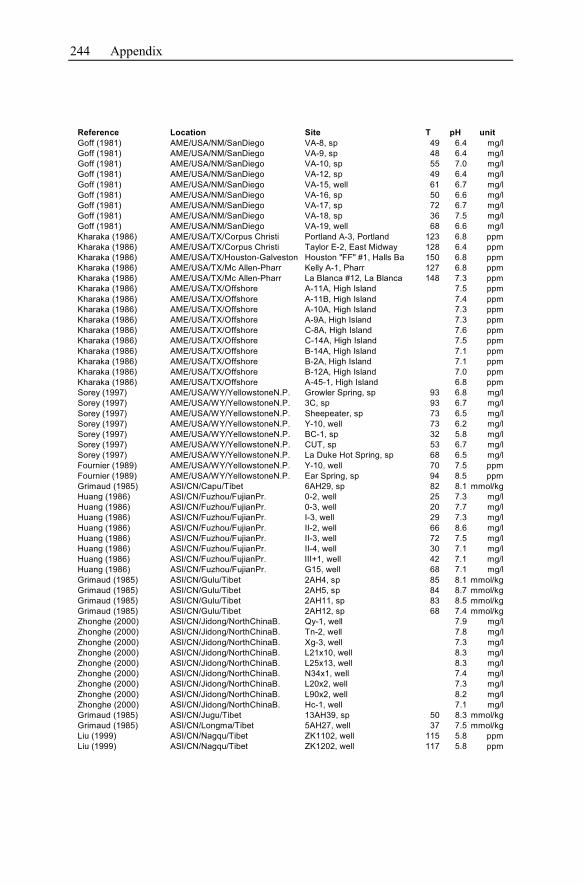
244 Appendix
Reference Location Site T pH unit
Goff (1981) AME/USA/NM/SanDiego VA-8, sp 49 6.4 mg/l
Goff (1981) AME/USA/NM/SanDiego VA-9, sp 48 6.4 mg/l
Goff (1981) AME/USA/NM/SanDiego VA-10, sp 55 7.0 mg/l
Goff (1981) AME/USA/NM/SanDiego VA-12, sp 49 6.4 mg/l
Goff (1981) AME/USA/NM/SanDiego VA-15, well 61 6.7 mg/l
Goff (1981) AME/USA/NM/SanDiego VA-16, sp 50 6.6 mg/l
Goff (1981) AME/USA/NM/SanDiego VA-17, sp 72 6.7 mg/l
Goff (1981) AME/USA/NM/SanDiego VA-18, sp 36 7.5 mg/l
Goff (1981) AME/USA/NM/SanDiego VA-19, well 68 6.6 mg/l
Kharaka (1986) AME/USA/TX/Corpus Christi Portland A-3, Portland 123 6.8 ppm
Kharaka (1986) AME/USA/TX/Corpus Christi Taylor E-2, East Midway 128 6.4 ppm
Kharaka (1986) AME/USA/TX/Houston-Galveston Houston "FF" #1, Halls Ba 150 6.8 ppm
Kharaka (1986) AME/USA/TX/Mc Allen-Pharr Kelly A-1, Pharr 127 6.8 ppm
Kharaka (1986) AME/USA/TX/Mc Allen-Pharr La Blanca #12, La Blanca 148 7.3 ppm
Kharaka (1986) AME/USA/TX/Offshore A-11A, High Island 7.5 ppm
Kharaka (1986) AME/USA/TX/Offshore A-11B, High Island 7.4 ppm
Kharaka (1986) AME/USA/TX/Offshore A-10A, High Island 7.3 ppm
Kharaka (1986) AME/USA/TX/Offshore A-9A, High Island 7.3 ppm
Kharaka (1986) AME/USA/TX/Offshore C-8A, High Island 7.6 ppm
Kharaka (1986) AME/USA/TX/Offshore C-14A, High Island 7.5 ppm
Kharaka (1986) AME/USA/TX/Offshore B-14A, High Island 7.1 ppm
Kharaka (1986) AME/USA/TX/Offshore B-2A, High Island 7.1 ppm
Kharaka (1986) AME/USA/TX/Offshore B-12A, High Island 7.0 ppm
Kharaka (1986) AME/USA/TX/Offshore A-45-1, High Island 6.8 ppm
Sorey (1997) AME/USA/WY/YellowstoneN.P. Growler Spring, sp 93 6.8 mg/l
Sorey (1997) AME/USA/WY/YellowstoneN.P. 3C, sp 93 6.7 mg/l
Sorey (1997) AME/USA/WY/YellowstoneN.P. Sheepeater, sp 73 6.5 mg/l
Sorey (1997) AME/USA/WY/YellowstoneN.P. Y-10, well 73 6.2 mg/l
Sorey (1997) AME/USA/WY/YellowstoneN.P. BC-1, sp 32 5.8 mg/l
Sorey (1997) AME/USA/WY/YellowstoneN.P. CUT, sp 53 6.7 mg/l
Sorey (1997) AME/USA/WY/YellowstoneN.P. La Duke Hot Spring, sp 68 6.5 mg/l
Fournier (1989) AME/USA/WY/YellowstoneN.P. Y-10, well 70 7.5 ppm
Fournier (1989) AME/USA/WY/YellowstoneN.P. Ear Spring, sp 94 8.5 ppm
Grimaud (1985) ASI/CN/Capu/Tibet 6AH29, sp 82 8.1 mmol/kg
Huang (1986) ASI/CN/Fuzhou/FujianPr. 0-2, well 25 7.3 mg/l
Huang (1986) ASI/CN/Fuzhou/FujianPr. 0-3, well 20 7.7 mg/l
Huang (1986) ASI/CN/Fuzhou/FujianPr. I-3, well 29 7.3 mg/l
Huang (1986) ASI/CN/Fuzhou/FujianPr. II-2, well 66 8.6 mg/l
Huang (1986) ASI/CN/Fuzhou/FujianPr. II-3, well 72 7.5 mg/l
Huang (1986) ASI/CN/Fuzhou/FujianPr. II-4, well 30 7.1 mg/l
Huang (1986) ASI/CN/Fuzhou/FujianPr. III+1, well 42 7.1 mg/l
Huang (1986) ASI/CN/Fuzhou/FujianPr. G15, well 68 7.1 mg/l
Grimaud (1985) ASI/CN/Gulu/Tibet 2AH4, sp 85 8.1 mmol/kg
Grimaud (1985) ASI/CN/Gulu/Tibet 2AH5, sp 84 8.7 mmol/kg
Grimaud (1985) ASI/CN/Gulu/Tibet 2AH11, sp 83 8.5 mmol/kg
Grimaud (1985) ASI/CN/Gulu/Tibet 2AH12, sp 68 7.4 mmol/kg
Zhonghe (2000) ASI/CN/Jidong/NorthChinaB. Qy-1, well 7.9 mg/l
Zhonghe (2000) ASI/CN/Jidong/NorthChinaB. Tn-2, well 7.8 mg/l
Zhonghe (2000) ASI/CN/Jidong/NorthChinaB. Xg-3, well 7.3 mg/l
Zhonghe (2000) ASI/CN/Jidong/NorthChinaB. L21x10, well 8.3 mg/l
Zhonghe (2000) ASI/CN/Jidong/NorthChinaB. L25x13, well 8.3 mg/l
Zhonghe (2000) ASI/CN/Jidong/NorthChinaB. N34x1, well 7.4 mg/l
Zhonghe (2000) ASI/CN/Jidong/NorthChinaB. L20x2, well 7.3 mg/l
Zhonghe (2000) ASI/CN/Jidong/NorthChinaB. L90x2, well 8.2 mg/l
Zhonghe (2000) ASI/CN/Jidong/NorthChinaB. Hc-1, well 7.1 mg/l
Grimaud (1985) ASI/CN/Jugu/Tibet 13AH39, sp 50 8.3 mmol/kg
Grimaud (1985) ASI/CN/Longma/Tibet 5AH27, well 37 7.5 mmol/kg
Liu (1999) ASI/CN/Nagqu/Tibet ZK1102, well 115 5.8 ppm
Liu (1999) ASI/CN/Nagqu/Tibet ZK1202, well 117 5.8 ppm
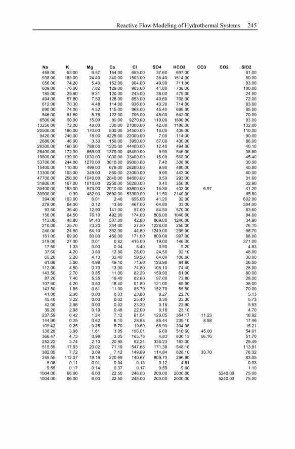
Reactive Flow Modeling of Hydrothermal Systems 245
Na K Mg Ca Cl SO4 HCO3 CO3 CO2 SIO2
458.00 53.00 9.57 154.00 653.00 37.60 697.00 81.00
938.00 183.00 24.40 340.00 1503.00 38.40 1514.00 50.00
656.00 74.20 5.40 152.00 904.00 40.90 711.00 93.00
609.00 70.00 7.82 129.00 903.00 41.80 738.00 100.00
185.00 29.90 9.31 120.00 243.00 38.00 479.00 24.00
494.00 57.80 7.50 128.00 653.00 40.60 708.00 72.00
612.00 70.30 4.48 114.00 936.00 43.20 714.00 83.00
690.00 74.00 4.52 115.00 968.00 45.40 699.00 85.00
546.00 61.60 5.76 122.00 705.00 45.00 642.00 70.00
6500.00 68.00 15.00 89.00 9270.00 110.00 1600.00 93.00
13250.00 72.00 48.00 330.00 21000.00 42.00 1180.00 132.00
20500.00 180.00 170.00 800.00 34500.00 16.00 409.00 110.00
9420.00 240.00 18.00 4225.00 22000.00 7.00 114.00 90.00
2680.00 46.00 3.30 150.00 3950.00 57.00 400.00 86.00
26300.00 160.00 788.00 1320.00 44400.00 12.40 494.00 40.10
28400.00 172.00 869.00 1370.00 48400.00 9.90 546.00 38.80
19800.00 139.00 1030.00 1030.00 33400.00 16.00 568.00 45.40
53700.00 244.00 1270.00 3810.00 99000.00 7.40 308.00 30.00
15400.00 110.00 499.00 679.00 26200.00 9.90 480.00 40.80
13300.00 103.00 349.00 850.00 23000.00 9.90 443.00 60.00
47700.00 250.00 1040.00 2840.00 84600.00 0.50 293.00 31.60
31800.00 167.00 1010.00 2250.00 56200.00 0.40 350.00 32.90
30400.00 183.00 873.00 2010.00 53800.00 15.30 402.00 6.97 41.20
30900.00 0.39 482.00 2690.00 53300.00 11.50 2140.00 65.80
394.00 103.00 0.01 2.40 695.00 41.20 32.00 602.00
278.00 64.00 0.12 13.60 467.00 64.80 33.00 304.00
93.50 36.40 12.90 141.00 97.00 84.50 570.00 83.60
156.00 64.50 76.10 492.00 174.00 808.00 1040.00 94.60
113.00 48.80 91.40 507.00 42.80 869.00 1240.00 34.90
210.00 25.70 73.20 334.00 37.50 1228.00 250.00 76.10
240.00 24.50 64.10 332.00 44.80 1249.00 295.00 56.70
161.00 69.00 80.00 450.00 171.00 800.00 997.00 88.00
319.00 27.00 0.01 0.82 415.00 19.00 146.00 371.00
17.50 1.33 0.00 0.04 8.40 0.90 9.20 4.83
37.60 4.20 3.89 12.80 28.00 24.50 92.10 48.00
65.20 2.20 4.13 32.40 59.50 64.80 100.60 30.00
61.60 5.00 4.98 49.10 71.60 123.90 84.80 26.00
112.00 4.50 0.73 13.00 74.80 105.10 74.40 28.00
143.50 2.70 0.85 11.00 82.20 159.90 61.00 80.00
87.20 7.40 5.35 19.40 82.60 97.00 73.80 28.00
107.60 4.20 3.80 18.40 91.80 121.00 65.90 36.00
143.50 1.85 0.61 11.00 85.70 152.70 55.50 70.00
41.00 2.98 0.00 0.03 23.80 0.27 22.70 5.13
45.40 3.22 0.00 0.02 25.40 0.30 25.30 5.73
42.00 2.98 0.00 0.02 23.30 0.18 22.90 5.83
39.20 2.98 0.19 0.48 22.00 0.18 23.10 4.70
237.59 0.42 1.24 7.12 81.54 120.05 364.17 11.23 16.92
144.90 0.25 0.62 6.10 28.83 85.44 239.10 8.98 17.46
109.42 0.25 0.25 5.70 19.60 66.90 204.96 15.21
338.28 3.98 1.61 3.05 196.01 6.69 510.60 45.00 54.01
366.47 4.73 0.99 3.05 163.73 4.83 630.13 56.16 51.70
252.22 3.74 2.10 20.95 92.24 336.23 183.00 29.49
515.59 17.93 20.02 71.19 547.68 171.38 548.16 113.81
382.05 7.72 3.09 7.12 149.89 114.84 628.10 33.70 78.32
245.55 112.07 19.16 220.69 140.67 809.73 296.90 83.05
5.08 0.11 0.01 0.04 0.13 0.12 4.81 0.93
9.55 0.17 0.14 0.37 0.17 0.59 9.60 1.10
1004.00 66.00 6.00 22.50 248.00 200.00 2000.00 5240.00 75.00
1004.00 66.00 6.00 22.50 248.00 200.00 2000.00 5240.00 75.00
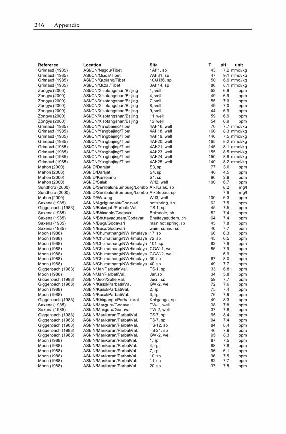
246 Appendix
Reference Location Site T pH unit
Grimaud (1985) ASI/CN/Nagqu/Tibet 1AH1, sp 43 7.2 mmol/kg
Grimaud (1985) ASI/CN/Qiaga/Tibet 7AH31, sp 47 9.1 mmol/kg
Grimaud (1985) ASI/CN/Quxiang/Tibet 10AH36, sp 50 6.9 mmol/kg
Grimaud (1985) ASI/CN/Quzai/Tibet 3AH14, sp 86 8.1 mmol/kg
Zongyu (2000) ASI/CN/Xiaotangshan/Beijing 1, well 52 6.9 ppm
Zongyu (2000) ASI/CN/Xiaotangshan/Beijing 4, well 49 6.9 ppm
Zongyu (2000) ASI/CN/Xiaotangshan/Beijing 7, well 55 7.0 ppm
Zongyu (2000) ASI/CN/Xiaotangshan/Beijing 8, well 49 7.0 ppm
Zongyu (2000) ASI/CN/Xiaotangshan/Beijing 9, well 44 6.9 ppm
Zongyu (2000) ASI/CN/Xiaotangshan/Beijing 11, well 59 6.9 ppm
Zongyu (2000) ASI/CN/Xiaotangshan/Beijing 12, well 54 6.9 ppm
Grimaud (1985) ASI/CN/Yangbajing/Tibet 4AH16, well 70 7.7 mmol/kg
Grimaud (1985) ASI/CN/Yangbajing/Tibet 4AH18, well 160 8.3 mmol/kg
Grimaud (1985) ASI/CN/Yangbajing/Tibet 4AH19, well 140 7.5 mmol/kg
Grimaud (1985) ASI/CN/Yangbajing/Tibet 4AH20, well 165 8.2 mmol/kg
Grimaud (1985) ASI/CN/Yangbajing/Tibet 4AH21, well 145 8.1 mmol/kg
Grimaud (1985) ASI/CN/Yangbajing/Tibet 4AH23, well 155 8.5 mmol/kg
Grimaud (1985) ASI/CN/Yangbajing/Tibet 4AH24, well 150 8.8 mmol/kg
Grimaud (1985) ASI/CN/Yangbajing/Tibet 4AH25, well 140 8.2 mmol/kg
Mahon (2000) ASI/ID/Darajat S3, sp 77 3.0 ppm
Mahon (2000) ASI/ID/Darajat S4, sp 40 4.5 ppm
Mahon (2000) ASI/ID/Kamojang S1, sp 96 2.9 ppm
Mahon (2000) ASI/ID/Salak W12, well 100 6.7 ppm
Sundhoro (2000) ASI/ID/SembalunBumbung/Lombo Aik Kalak, sp 8.2 mg/l
Sundhoro (2000) ASI/ID/SembalunBumbung/Lombo Aik Sebau, sp 7.6 mg/l
Mahon (2000) ASI/ID/Wayang W13, well 100 6.3 ppm
Saxena (1985) ASI/IN/Agnigundala/Godavari hot spring, sp 62 7.5 ppm
Giggenbach (1983) ASI/IN/Balargah/ParbatinVal. TS-1, sp 45 7.5 ppm
Saxena (1985) ASI/IN/Bhimdole/Godavari Bhimdole, bh 52 7.4 ppm
Saxena (1985) ASI/IN/Bhuttayagudem/Godavar Bhuttayagudem, bh 64 7.4 ppm
Saxena (1985) ASI/IN/Buga/Godavari main hot spring, sp 45 7.8 ppm
Saxena (1985) ASI/IN/Buga/Godavari warm spring, sp 40 7.7 ppm
Moon (1988) ASI/IN/Chumathang/NWHimalaya 17, sp 66 6.3 ppm
Moon (1988) ASI/IN/Chumathang/NWHimalaya 72, sp 45 6.5 ppm
Moon (1988) ASI/IN/Chumathang/NWHimalaya 101, sp 83 7.6 ppm
Moon (1988) ASI/IN/Chumathang/NWHimalaya CGW-1, well 85 7.9 ppm
Moon (1988) ASI/IN/Chumathang/NWHimalaya CGW-2, well 6.9 ppm
Moon (1988) ASI/IN/Chumathang/NWHimalaya 39, sp 87 8.0 ppm
Moon (1988) ASI/IN/Chumathang/NWHimalaya 40, sp 49 7.7 ppm
Giggenbach (1983) ASI/IN/Jan/ParbatinVal. TS-1, sp 33 6.8 ppm
Moon (1988) ASI/IN/Jan/ParbatiVal. Jan,sp 34 5.8 ppm
Giggenbach (1983) ASI/IN/Jeori/SutlejVal. Jeori, sp 59 7.7 ppm
Giggenbach (1983) ASI/IN/Kasol/ParbatinVal. GW-2, well 72 7.6 ppm
Moon (1988) ASI/IN/Kasol/ParbatiVal. 2, sp 75 7.4 ppm
Moon (1988) ASI/IN/Kasol/ParbatiVal. 3, sp 76 7.9 ppm
Giggenbach (1983) ASI/IN/Khirganga/ParbatinVal Khirganga, sp 49 8.3 ppm
Saxena (1985) ASI/IN/Manguru/Godavari TW-1, well 38 7.8 ppm
Saxena (1985) ASI/IN/Manguru/Godavari TW-2, well 37 7.8 ppm
Giggenbach (1983) ASI/IN/Manikaran/ParbatiVal. TS-7, sp 95 8.4 ppm
Giggenbach (1983) ASI/IN/Manikaran/ParbatiVal. TS-7, sp 94 7.4 ppm
Giggenbach (1983) ASI/IN/Manikaran/ParbatiVal. TS-12, sp 84 8.4 ppm
Giggenbach (1983) ASI/IN/Manikaran/ParbatiVal. TS-21, sp 46 7.9 ppm
Giggenbach (1983) ASI/IN/Manikaran/ParbatiVal. GW-2, well 95 8.3 ppm
Moon (1988) ASI/IN/Manikaran/ParbatVal. 1, sp 87 7.5 ppm
Moon (1988) ASI/IN/Manikaran/ParbatVal. 4, sp 88 7.6 ppm
Moon (1988) ASI/IN/Manikaran/ParbatVal. 7, sp 96 6.1 ppm
Moon (1988) ASI/IN/Manikaran/ParbatVal. 10, sp 96 7.5 ppm
Moon (1988) ASI/IN/Manikaran/ParbatVal. 11, sp 82 7.7 ppm
Moon (1988) ASI/IN/Manikaran/ParbatVal. 20, sp 37 7.5 ppm
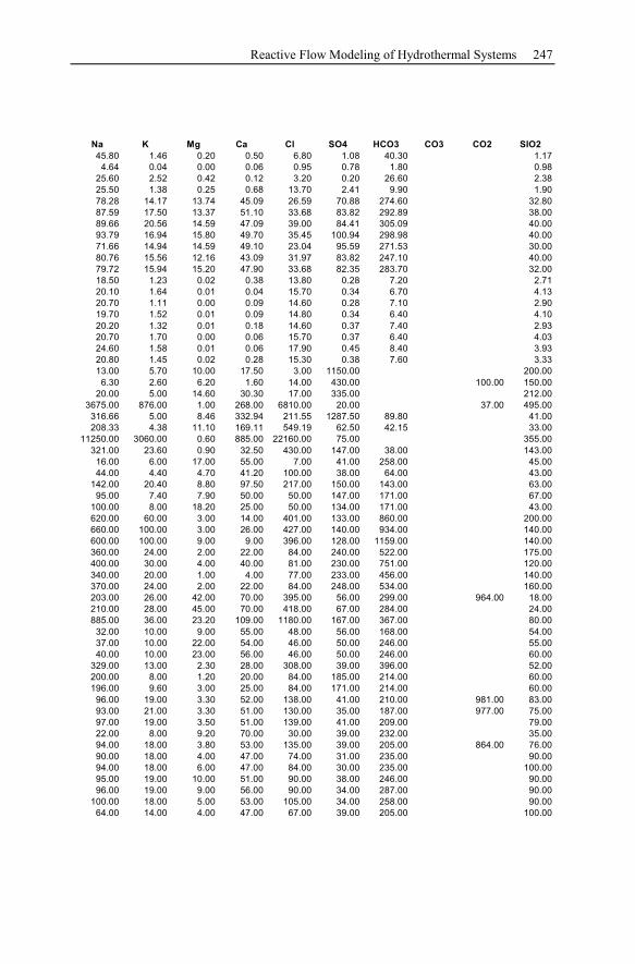
Reactive Flow Modeling of Hydrothermal Systems 247
Na K Mg Ca Cl SO4 HCO3 CO3 CO2 SIO2
45.80 1.46 0.20 0.50 6.80 1.08 40.30 1.17
4.64 0.04 0.00 0.06 0.95 0.78 1.80 0.98
25.60 2.52 0.42 0.12 3.20 0.20 26.60 2.38
25.50 1.38 0.25 0.68 13.70 2.41 9.90 1.90
78.28 14.17 13.74 45.09 26.59 70.88 274.60 32.80
87.59 17.50 13.37 51.10 33.68 83.82 292.89 38.00
89.66 20.56 14.59 47.09 39.00 84.41 305.09 40.00
93.79 16.94 15.80 49.70 35.45 100.94 298.98 40.00
71.66 14.94 14.59 49.10 23.04 95.59 271.53 30.00
80.76 15.56 12.16 43.09 31.97 83.82 247.10 40.00
79.72 15.94 15.20 47.90 33.68 82.35 283.70 32.00
18.50 1.23 0.02 0.38 13.80 0.28 7.20 2.71
20.10 1.64 0.01 0.04 15.70 0.34 6.70 4.13
20.70 1.11 0.00 0.09 14.60 0.28 7.10 2.90
19.70 1.52 0.01 0.09 14.80 0.34 6.40 4.10
20.20 1.32 0.01 0.18 14.60 0.37 7.40 2.93
20.70 1.70 0.00 0.06 15.70 0.37 6.40 4.03
24.60 1.58 0.01 0.06 17.90 0.45 8.40 3.93
20.80 1.45 0.02 0.28 15.30 0.38 7.60 3.33
13.00 5.70 10.00 17.50 3.00 1150.00 200.00
6.30 2.60 6.20 1.60 14.00 430.00 100.00 150.00
20.00 5.00 14.60 30.30 17.00 335.00 212.00
3675.00 876.00 1.00 268.00 6810.00 20.00 37.00 495.00
316.66 5.00 8.46 332.94 211.55 1287.50 89.80 41.00
208.33 4.38 11.10 169.11 549.19 62.50 42.15 33.00
11250.00 3060.00 0.60 885.00 22160.00 75.00 355.00
321.00 23.60 0.90 32.50 430.00 147.00 38.00 143.00
16.00 6.00 17.00 55.00 7.00 41.00 258.00 45.00
44.00 4.40 4.70 41.20 100.00 38.00 64.00 43.00
142.00 20.40 8.80 97.50 217.00 150.00 143.00 63.00
95.00 7.40 7.90 50.00 50.00 147.00 171.00 67.00
100.00 8.00 18.20 25.00 50.00 134.00 171.00 43.00
620.00 60.00 3.00 14.00 401.00 133.00 860.00 200.00
660.00 100.00 3.00 26.00 427.00 140.00 934.00 140.00
600.00 100.00 9.00 9.00 396.00 128.00 1159.00 140.00
360.00 24.00 2.00 22.00 84.00 240.00 522.00 175.00
400.00 30.00 4.00 40.00 81.00 230.00 751.00 120.00
340.00 20.00 1.00 4.00 77.00 233.00 456.00 140.00
370.00 24.00 2.00 22.00 84.00 248.00 534.00 160.00
203.00 26.00 42.00 70.00 395.00 56.00 299.00 964.00 18.00
210.00 28.00 45.00 70.00 418.00 67.00 284.00 24.00
885.00 36.00 23.20 109.00 1180.00 167.00 367.00 80.00
32.00 10.00 9.00 55.00 48.00 56.00 168.00 54.00
37.00 10.00 22.00 54.00 46.00 50.00 246.00 55.00
40.00 10.00 23.00 56.00 46.00 50.00 246.00 60.00
329.00 13.00 2.30 28.00 308.00 39.00 396.00 52.00
200.00 8.00 1.20 20.00 84.00 185.00 214.00 60.00
196.00 9.60 3.00 25.00 84.00 171.00 214.00 60.00
96.00 19.00 3.30 52.00 138.00 41.00 210.00 981.00 83.00
93.00 21.00 3.30 51.00 130.00 35.00 187.00 977.00 75.00
97.00 19.00 3.50 51.00 139.00 41.00 209.00 79.00
22.00 8.00 9.20 70.00 30.00 39.00 232.00 35.00
94.00 18.00 3.80 53.00 135.00 39.00 205.00 864.00 76.00
90.00 18.00 4.00 47.00 74.00 31.00 235.00 90.00
94.00 18.00 6.00 47.00 84.00 30.00 235.00 100.00
95.00 19.00 10.00 51.00 90.00 38.00 246.00 90.00
96.00 19.00 9.00 56.00 90.00 34.00 287.00 90.00
100.00 18.00 5.00 53.00 105.00 34.00 258.00 90.00
64.00 14.00 4.00 47.00 67.00 39.00 205.00 100.00
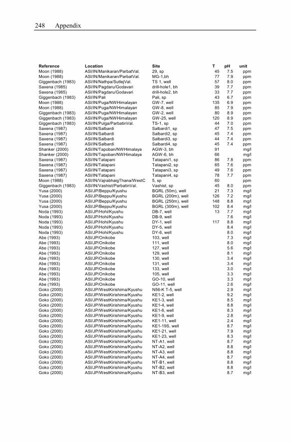
248 Appendix
Reference Location Site T pH unit
Moon (1988) ASI/IN/Manikaran/ParbatVal. 29, sp 45 7.5 ppm
Moon (1988) ASI/IN/Manikaran/ParbatVal. MG-1,bh 77 7.9 ppm
Giggenbach (1983) ASI/IN/Nathpa/SutlejVal. TS 1, well 57 8.0 ppm
Saxena (1985) ASI/IN/Pagdaru/Godavari drill-hole1, bh 39 7.7 ppm
Saxena (1985) ASI/IN/Pagdaru/Godavari drill-hole2, bh 33 7.7 ppm
Giggenbach (1983) ASI/IN/Pali Pali, sp 43 6.7 ppm
Moon (1988) ASI/IN/Puga/NWHimalayan GW-7, well 135 6.9 ppm
Moon (1988) ASI/IN/Puga/NWHimalayan GW-8, well 85 7.9 ppm
Giggenbach (1983) ASI/IN/Puga/NWHimalayan GW-2, well 80 8.9 ppm
Giggenbach (1983) ASI/IN/Puga/NWHimalayan GW-25, well 120 8.9 ppm
Giggenbach (1983) ASI/IN/Pulga/ParbatinVal. TS-1, sp 44 7.0 ppm
Saxena (1987) ASI/IN/Salbardi Salbardi1, sp 47 7.5 ppm
Saxena (1987) ASI/IN/Salbardi Salbardi2, sp 45 7.4 ppm
Saxena (1987) ASI/IN/Salbardi Salbardi3, sp 44 7.4 ppm
Saxena (1987) ASI/IN/Salbardi Salbardi4, sp 45 7.4 ppm
Shanker (2000) ASI/IN/Tapoban/NWHimalaya AGW-3, bh 91 mg/l
Shanker (2000) ASI/IN/Tapoban/NWHimalaya AGW-6, bh 66 mg/l
Saxena (1987) ASI/IN/Tatapani Tatapani1, sp 86 7.8 ppm
Saxena (1987) ASI/IN/Tatapani Tatapani2, sp 65 7.6 ppm
Saxena (1987) ASI/IN/Tatapani Tatapani3, sp 49 7.6 ppm
Saxena (1987) ASI/IN/Tatapani Tatapani4, sp 78 7.7 ppm
Moon (1988) ASI/IN/VajrabhaigThana/WestC 5, sp 60 ppm
Giggenbach (1983) ASI/IN/Vashist/ParbatinVal. Vashist, sp 45 8.0 ppm
Yusa (2000) ASI/JP/Beppu/Kyushu BGRL (50m), well 21 7.3 mg/l
Yusa (2000) ASI/JP/Beppu/Kyushu BGRL (200m), well 126 7.2 mg/l
Yusa (2000) ASI/JP/Beppu/Kyushu BGRL (250m), well 148 8.8 mg/l
Yusa (2000) ASI/JP/Beppu/Kyushu BGRL (300m), well 102 8.4 mg/l
Noda (1993) ASI/JP/Hohi/Kyushu DB-7, well 13 7.7 mg/l
Noda (1993) ASI/JP/Hohi/Kyushu DB-9, well 7.6 mg/l
Noda (1993) ASI/JP/Hohi/Kyushu DY-1, well 117 8.8 mg/l
Noda (1993) ASI/JP/Hohi/Kyushu DY-5, well 8.4 mg/l
Noda (1993) ASI/JP/Hohi/Kyushu DY-6, well 8.0 mg/l
Abe (1993) ASI/JP/Onikobe 103, well 7.3 mg/l
Abe (1993) ASI/JP/Onikobe 111, well 8.0 mg/l
Abe (1993) ASI/JP/Onikobe 127, well 5.6 mg/l
Abe (1993) ASI/JP/Onikobe 129, well 8.1 mg/l
Abe (1993) ASI/JP/Onikobe 130, well 3.4 mg/l
Abe (1993) ASI/JP/Onikobe 131, well 3.4 mg/l
Abe (1993) ASI/JP/Onikobe 133, well 3.0 mg/l
Abe (1993) ASI/JP/Onikobe 105, well 3.3 mg/l
Abe (1993) ASI/JP/Onikobe GO-10, well 3.3 mg/l
Abe (1993) ASI/JP/Onikobe GO-11, well 2.6 mg/l
Goko (2000) ASI/JP/WestKirishima/Kyushu N56-K T-5, well 2.9 mg/l
Goko (2000) ASI/JP/WestKirishima/Kyushu KE1-2, well 9.2 mg/l
Goko (2000) ASI/JP/WestKirishima/Kyushu KE1-3, well 8.5 mg/l
Goko (2000) ASI/JP/WestKirishima/Kyushu KE1-4, well 8.8 mg/l
Goko (2000) ASI/JP/WestKirishima/Kyushu KE1-6, well 8.3 mg/l
Goko (2000) ASI/JP/WestKirishima/Kyushu KE1-9, well 2.8 mg/l
Goko (2000) ASI/JP/WestKirishima/Kyushu KE1-11, well 2.4 mg/l
Goko (2000) ASI/JP/WestKirishima/Kyushu KE1-19S, well 8.7 mg/l
Goko (2000) ASI/JP/WestKirishima/Kyushu KE1-21, well 7.9 mg/l
Goko (2000) ASI/JP/WestKirishima/Kyushu KE1-23, well 8.3 mg/l
Goko (2000) ASI/JP/WestKirishima/Kyushu NT-A1, well 8.7 mg/l
Goko (2000) ASI/JP/WestKirishima/Kyushu NT-A2, well 8.8 mg/l
Goko (2000) ASI/JP/WestKirishima/Kyushu NT-A3, well 8.8 mg/l
Goko (2000) ASI/JP/WestKirishima/Kyushu NT-A4, well 8.7 mg/l
Goko (2000) ASI/JP/WestKirishima/Kyushu NT-B1, well 8.8 mg/l
Goko (2000) ASI/JP/WestKirishima/Kyushu NT-B2, well 8.8 mg/l
Goko (2000) ASI/JP/WestKirishima/Kyushu NT-B3, well 8.7 mg/l
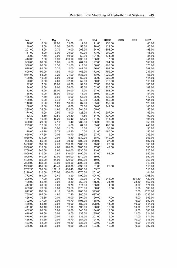
Reactive Flow Modeling of Hydrothermal Systems 249
Na K Mg Ca Cl SO4 HCO3 CO3 CO2 SIO2
16.00 6.00 17.00 55.00 7.00 41.00 258.00 45.00
40.00 12.00 6.00 36.00 53.00 28.00 129.00 60.00
201.00 13.00 0.70 19.00 206.00 24.00 303.00 98.00
111.00 8.90 3.00 25.00 50.00 73.00 200.00 48.00
95.00 7.40 7.90 50.00 50.00 121.00 171.00 35.00
413.00 7.00 0.90 490.00 1490.00 136.00 7.00 41.00
580.00 80.00 1.00 5.00 464.00 127.00 884.00 160.00
580.00 80.00 1.30 11.00 411.00 100.00 903.00 175.00
618.00 81.00 0.20 2.00 447.00 156.00 704.00 207.00
600.00 90.00 1.50 5.00 468.00 172.00 799.00 237.00
1044.00 68.00 7.20 21.00 1135.00 43.00 1020.00 68.00
100.00 10.00 6.00 30.00 60.00 35.00 220.00 114.00
90.00 8.00 7.00 32.00 52.00 30.00 218.00 110.00
92.00 7.00 10.00 40.00 52.00 57.00 232.00 105.00
94.00 8.00 9.00 38.00 58.00 52.00 225.00 102.00
12.00 6.00 26.00 90.00 15.00 27.00 363.00 91.00
15.00 9.00 25.00 95.00 15.00 30.00 380.00 84.00
135.00 7.50 0.60 5.00 67.00 85.00 132.00 142.00
130.00 6.20 0.40 7.50 50.00 105.00 150.00 131.00
140.00 8.00 1.20 10.00 67.00 105.00 150.00 128.00
138.00 8.00 0.80 6.00 71.00 80.00 142.00 140.00
285.00 32.00 1.60 152.00 704.00 155.00 55.00
174.00 9.00 0.50 8.00 123.00 73.00 207.00 69.00
32.30 3.60 10.50 20.50 17.50 34.00 127.00 99.00
154.00 16.80 48.20 65.40 65.70 84.00 714.00 191.00
380.00 23.00 7.10 1.40 282.00 166.00 390.00 353.00
229.00 17.90 6.10 5.80 64.60 85.00 487.00 246.00
5.40 2.20 3.00 11.70 3.00 1.50 56.90 50.20
170.00 48.10 5.73 45.90 0.30 181.00 460.00 150.00
625.00 47.20 0.05 40.70 998.00 67.50 19.00 283.00
1060.00 134.00 0.01 8.80 1630.00 58.60 149.00 663.00
995.00 85.80 0.34 39.30 1600.00 230.00 27.00 597.00
1400.00 250.00 2.70 290.00 2780.00 75.00 25.00 360.00
1300.00 210.00 4.60 320.00 2780.00 77.00 49.00 380.00
1700.00 340.00 2.60 340.00 3630.00 13.00 720.00
1900.00 310.00 0.81 310.00 3490.00 17.00 61.00 650.00
1900.00 440.00 33.00 450.00 4910.00 19.00 690.00
1400.00 360.00 34.00 470.00 4480.00 19.00 660.00
2000.00 430.00 63.00 650.00 4600.00 33.00 610.00
1950.00 439.00 48.40 408.00 5630.00 31.00 28.00 515.00
1787.50 503.50 137.10 408.40 5286.00 55.20 510.00
3120.00 810.00 270.00 1460.00 9570.00 201.00 144.00
772.00 161.00 2.40 3.90 1190.00 404.00 1008.00
200.00 17.00 0.01 0.30 32.00 194.00 244.00 191.40 422.00
420.00 55.60 0.01 8.30 660.00 145.00 31.50 23.30 567.00
417.00 61.00 0.01 9.70 571.00 156.00 4.00 3.00 574.00
653.00 78.30 0.01 19.50 1075.00 80.00 2.50 1.90 508.00
842.00 196.00 2.10 10.80 1205.00 375.00 2.60 1023.00
765.00 167.00 4.80 17.40 980.00 697.00 1.80 1036.00
456.00 76.30 0.01 16.00 594.00 190.00 7.00 5.00 609.00
702.00 77.90 0.01 40.70 1198.00 188.00 7.00 6.00 602.00
439.00 53.40 0.01 19.90 582.00 228.00 14.00 10.00 544.00
441.00 53.40 0.01 11.00 596.00 198.00 16.00 10.00 628.00
452.00 63.00 0.01 10.00 640.00 194.00 12.00 9.00 603.00
478.00 64.60 0.01 9.70 633.00 195.00 16.00 11.00 614.00
478.00 61.30 0.01 11.50 635.00 201.00 9.00 7.00 571.00
466.00 64.80 0.01 9.70 654.00 194.00 13.00 10.00 615.00
483.00 64.90 0.01 10.10 633.00 193.00 12.00 9.00 611.00
475.00 64.30 0.01 9.90 626.00 194.00 12.00 9.00 602.00
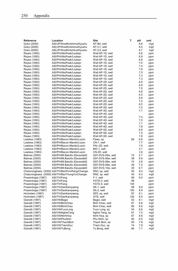
250 Appendix
Reference Location Site T pH unit
Goko (2000) ASI/JP/WestKirishima/Kyushu NT-B4, well 8.6 mg/l
Goko (2000) ASI/JP/WestKirishima/Kyushu NT-C1, well 8.5 mg/l
Goko (2000) ASI/JP/WestKirishima/Kyushu NT-C2, well 8.7 mg/l
Reyes (1993) ASI/PH/AltoPeak/Leytepr. Well AP-1D, well 6.6 ppm
Reyes (1993) ASI/PH/AltoPeak/Leytepr. Well AP-1D, well 6.9 ppm
Reyes (1993) ASI/PH/AltoPeak/Leytepr. Well AP-1D, well 6.8 ppm
Reyes (1993) ASI/PH/AltoPeak/Leytepr. Well AP-1D, well 7.0 ppm
Reyes (1993) ASI/PH/AltoPeak/Leytepr. Well AP-1D, well 7.0 ppm
Reyes (1993) ASI/PH/AltoPeak/Leytepr. Well AP-1D, well 7.6 ppm
Reyes (1993) ASI/PH/AltoPeak/Leytepr. Well AP-1D, well 7.5 ppm
Reyes (1993) ASI/PH/AltoPeak/Leytepr. Well AP-1D, well 7.3 ppm
Reyes (1993) ASI/PH/AltoPeak/Leytepr. Well AP-1D, well 7.3 ppm
Reyes (1993) ASI/PH/AltoPeak/Leytepr. Well AP-2D, well 6.6 ppm
Reyes (1993) ASI/PH/AltoPeak/Leytepr. Well AP-2D, well 6.9 ppm
Reyes (1993) ASI/PH/AltoPeak/Leytepr. Well AP-2D, well 7.0 ppm
Reyes (1993) ASI/PH/AltoPeak/Leytepr. Well AP-2D, well 6.6 ppm
Reyes (1993) ASI/PH/AltoPeak/Leytepr. Well AP-2D, well 6.5 ppm
Reyes (1993) ASI/PH/AltoPeak/Leytepr. Well AP-2D, well 6.6 ppm
Reyes (1993) ASI/PH/AltoPeak/Leytepr. Well AP-2D, well 7.2 ppm
Reyes (1993) ASI/PH/AltoPeak/Leytepr. Well AP-2D, well 6.5 ppm
Reyes (1993) ASI/PH/AltoPeak/Leytepr. Well AP-2D, well 7.0 ppm
Reyes (1993) ASI/PH/AltoPeak/Leytepr. Well AP-4D, well 7.1 ppm
Reyes (1993) ASI/PH/AltoPeak/Leytepr. Well AP-4D, well ppm
Reyes (1993) ASI/PH/AltoPeak/Leytepr. Well AP-4D, well 7.4 ppm
Reyes (1993) ASI/PH/AltoPeak/Leytepr. Well AP-4D, well 7.0 ppm
Reyes (1993) ASI/PH/AltoPeak/Leytepr. Well AP-4D, well 7.1 ppm
Reyes (1993) ASI/PH/AltoPeak/Leytepr. Well AP-4D, well 7.6 ppm
Reyes (1993) ASI/PH/AltoPeak/Leytepr. Well AP-5D, well 6.9 ppm
Reyes (1993) ASI/PH/AltoPeak/Leytepr. Well AP-5D, well 7.0 ppm
Reyes (1993) ASI/PH/AltoPeak/Leytepr. Well AP-5D, well 7.8 ppm
Lawless (1983) ASI/PH/Bacon-Manito/Luzon Pawa, sp 66 6.6 ppm
Lawless (1983) ASI/PH/Bacon-Manito/Luzon CN-1, well 7.7 ppm
Lawless (1983) ASI/PH/Bacon-Manito/Luzon PAL-2D, well 7.0 ppm
Lawless (1983) ASI/PH/Bacon-Manito/Luzon MO-1, well 3.1 ppm
Lawless (1983) ASI/PH/Bacon-Manito/Luzon CN-2D, well 3.6 ppm
Balmes (2000) ASI/PH/Mt.BalutIs./DavaodelS G97-DVS-05w, well 75 2.7 ppm
Balmes (2000) ASI/PH/Mt.BalutIs./DavaodelS G97-DVS-06w, well 38 6.9 ppm
Balmes (2000) ASI/PH/Mt.BalutIs./DavaodelS G97-DVS-08w, well 74 2.8 ppm
Balmes (2000) ASI/PH/Mt.BalutIs./DavaodelS G97-DVS-09w, well 29 7.3 ppm
Balmes (2000) ASI/PH/Mt.BalutIs./DavaodelS G97-DVS-10w, well 39 6.7 ppm
Chaturongkawa. (2000) ASI/TH/BanPornRang/Changw. RN3, sp, well 55 8.4 mg/l
Chaturongkawa. (2000) ASI/TH/BanThungYo/Changw. RN2, sp, well 40 8.3 mg/l
Praserdvigai (1987) ASI/TH/Fang F-1, well 99 9.0 ppm
Praserdvigai (1987) ASI/TH/Fang FGTE-3, well 98 ppm
Praserdvigai (1987) ASI/TH/Fang FGTE-5, well 105 ppm
Praserdvigai (1987) ASI/TH/SanKampaeng SK-1, well 98 8.9 ppm
Praserdvigai (1987) ASI/TH/SanKampaeng SK-2, well 100 8.9 ppm
Hochstein (1987) ASI/TH/SanKampaeng SP5, sp, well 97 8.1 ppm
Hochstein (1987) ASI/TH/SanKampaeng GTE, well 120 8.5 ppm
Gianelli (1997) ASI/VN/Bagoi Bagoi, well 42 8.1 mg/l
Gianelli (1997) ASI/VN/BinhChau Binh Chau, well 81 6.8 mg/l
Gianelli (1997) ASI/VN/BinhChau Binh Chau, well 66 6.6 mg/l
Gianelli (1997) ASI/VN/FuocLong Fuoc Long, sp 54 8.6 mg/l
Gianelli (1997) ASI/VN/NghiaTang Nghia Tang, sp 67 7.5 mg/l
Gianelli (1997) ASI/VN/NinhHoa Ninh Hoa, sp 67 8.9 mg/l
Gianelli (1997) ASI/VN/PhuNinh Phu Ninh, sp 65 6.5 mg/l
Gianelli (1997) ASI/VN/ThachBich Thach Bich, sp 65 7.8 mg/l
Gianelli (1997) ASI/VN/TriemDuc Triem Duc, sp 74 7.9 mg/l
Gianelli (1997) ASI/VN/TuBong Tu Bong, well 66 7.1 mg/l
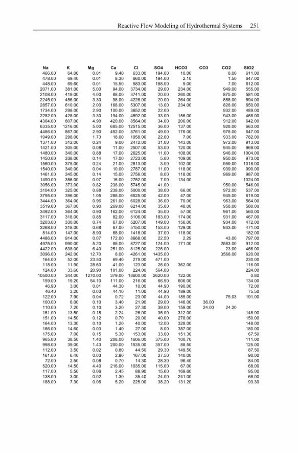
Reactive Flow Modeling of Hydrothermal Systems 251
Na K Mg Ca Cl SO4 HCO3 CO3 CO2 SIO2
466.00 64.00 0.01 9.40 633.00 194.00 10.00 8.00 611.00
478.00 69.40 0.01 8.30 660.00 194.00 2.10 1.50 647.00
448.00 69.60 0.01 15.50 583.00 188.00 9.00 7.00 612.00
2071.00 381.00 5.00 94.00 3734.00 29.00 234.00 949.00 555.00
2108.00 419.00 4.00 88.00 3741.00 20.00 260.00 875.00 581.00
2245.00 456.00 3.30 98.00 4226.00 20.00 264.00 858.00 594.00
2857.00 610.00 2.00 168.00 5307.00 13.00 234.00 828.00 650.00
1734.00 298.00 2.90 100.00 3652.00 22.00 932.00 489.00
2282.00 428.00 3.30 194.00 4592.00 33.00 156.00 943.00 468.00
4304.00 807.00 4.90 420.00 8564.00 34.00 206.00 912.00 642.00
6335.00 1216.00 5.00 685.00 12515.00 36.00 137.00 928.00 663.00
4466.00 867.00 2.90 452.00 8761.00 49.00 176.00 978.00 647.00
1049.00 298.00 1.73 18.00 1958.00 22.00 7.00 933.00 782.00
1371.00 312.00 0.24 9.00 2472.00 31.00 143.00 972.00 913.00
1421.00 305.00 0.08 11.00 2507.00 53.00 120.00 945.00 969.00
1480.00 340.00 0.88 17.00 2625.00 11.00 108.00 946.00 1004.00
1450.00 338.00 0.14 17.00 2723.00 5.00 109.00 950.00 973.00
1560.00 375.00 0.24 21.00 2813.00 3.00 102.00 959.00 1018.00
1540.00 340.00 0.04 10.00 2787.00 11.00 118.00 939.00 990.00
1461.00 345.00 0.14 15.00 2756.00 8.00 118.00 969.00 987.00
1490.00 356.00 0.07 16.00 2752.00 7.00 134.00 1024.00
3056.00 373.00 0.82 238.00 5745.00 41.00 950.00 546.00
3104.00 325.00 0.88 238.00 5000.00 38.00 66.00 972.00 537.00
3795.00 396.00 1.05 288.00 6525.00 42.00 47.00 945.00 619.00
3444.00 364.00 0.96 261.00 6028.00 36.00 70.00 963.00 564.00
3519.00 367.00 0.90 269.00 6214.00 35.00 48.00 958.00 580.00
3492.00 364.00 0.90 162.00 6124.00 35.00 57.00 961.00 560.00
3117.00 318.00 0.85 82.00 5106.00 183.00 174.00 931.00 467.00
3203.00 330.00 0.74 67.00 5207.00 149.00 156.00 934.00 472.00
3268.00 318.00 0.68 67.00 5150.00 153.00 129.00 933.00 471.00
814.00 147.00 8.90 68.00 1418.00 37.00 118.00 182.00
4486.00 914.00 0.07 172.00 8668.00 22.50 2.29 43.00 797.00
4975.00 990.00 5.20 85.00 8727.00 124.00 171.00 2583.00 912.00
4422.00 638.00 6.40 251.00 8125.00 226.00 23.00 466.00
3096.00 242.00 12.70 8.00 4261.00 1435.00 3568.00 620.00
164.00 52.00 23.50 69.40 279.00 471.00 230.00
118.00 11.90 28.60 41.00 123.00 26.00 362.00 116.00
124.00 33.60 20.90 101.00 224.00 564.00 224.00
10500.00 344.00 1270.00 379.00 18600.00 2620.00 122.00 0.80
159.00 19.20 54.10 111.00 216.00 66.90 606.00 134.00
46.90 3.00 0.01 44.30 10.00 44.90 190.00 72.00
46.40 3.20 0.03 44.10 11.00 44.90 189.00 75.50
122.00 7.90 0.04 0.72 23.00 44.00 185.00 75.03 191.00
100.00 6.00 0.10 3.40 21.90 29.00 146.00 36.00
110.00 7.20 0.10 3.20 27.30 39.00 159.00 24.00 24.20
151.00 13.50 0.18 2.24 26.00 35.00 312.00 148.00
151.00 14.50 0.12 0.70 20.00 40.00 278.00 150.00
164.00 13.30 0.10 1.20 40.00 12.00 328.00 148.00
166.00 14.60 0.03 1.40 27.00 8.00 387.00 180.00
175.00 7.00 0.15 5.30 153.00 33.00 151.30 67.50
965.00 38.50 1.40 208.00 1606.00 375.00 100.70 111.00
998.00 39.00 1.43 200.00 1535.00 357.00 88.50 125.00
112.00 3.50 0.02 0.80 44.50 29.30 149.50 87.50
161.00 6.40 0.03 2.90 167.00 27.50 140.00 90.00
72.00 2.50 0.08 0.70 14.30 28.30 96.40 84.00
520.00 14.50 4.40 216.00 1035.00 115.00 67.00 68.00
117.00 5.50 0.06 2.45 88.90 15.60 169.60 95.00
138.00 3.00 0.02 1.30 35.40 24.00 241.00 68.00
188.00 7.30 0.06 5.20 225.00 38.20 131.20 93.30
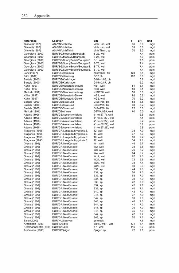
252 Appendix
Reference Location Site T pH unit
Gianelli (1997) ASI/VN/VinhHao Vinh Hao, well 36 6.9 mg/l
Gianelli (1997) ASI/VN/VinhHao Vinh Hao, well 33 6.6 mg/l
Gianelli (1997) ASI/VN/VinhThinh Vinh Thinh, sp 70 8.0 mg/l
Georgieva (2000) EUR/BG/Medovo/BourgasB. B-22, well 7.4 ppm
Georgieva (2000) EUR/BG/Medovo/BourgasB. B-25, well 7.0 ppm
Georgieva (2000) EUR/BG/SunnyBeach/BourgasB. B-1, well 7.5 ppm
Georgieva (2000) EUR/BG/SunnyBeach/BourgasB. B-76, well 7.4 ppm
Georgieva (2000) EUR/BG/SunnyBeach/BourgasB. B-77, well 7.4 ppm
Georgieva (2000) EUR/BG/SunnyBeach/BourgasB. B-79, well 7.4 ppm
Lenz (1997) EUR/DE/Hamburg Allermöhe, bh 123 6.4 mg/l
Fritz (1989) EUR/DE/Hamburg GB2,bh 102 6.0 mg/l
Bartels (2000) EUR/DE/Karlshagen GtKhn1/88, bh 5.2 mg/l
Bartels (2000) EUR/DE/Karlshagen GtKhn2/87, bh 5.2 mg/l
Kühn (1997) EUR/DE/Neubrandenburg NB1, well 51 6.1 mg/l
Kühn (1997) EUR/DE/Neubrandenburg NB3, well 50 6.1 mg/l
Merkel (1991) EUR/DE/Neubrandenburg N1GT86, well 53 6.0 mg/l
Kühn (1997) EUR/DE/Neustadt-Glewe NG1, well 92 5.2 mg/l
Kühn (1997) EUR/DE/Neustadt-Glewe NG2, well 70 5.2 mg/l
Bartels (2000) EUR/DE/Stralsund GtSs1/85, bh 58 5.5 mg/l
Bartels (2000) EUR/DE/Stralsund GtSs2/85, bh 30 5.2 mg/l
Bartels (2000) EUR/DE/Stralsund GtSs6/89, bh 22 6.0 mg/l
Merkel (1991) EUR/DE/Waren GTWA1/89, well 60 6.0 mg/l
Adams (1996) EUR/GB/AscensionIsland #1(ws87-7), well 5.5 ppm
Adams (1996) EUR/GB/AscensionIsland #1(ws87-20), well 7.1 ppm
Adams (1996) EUR/GB/AscensionIsland #1(ws87-22), well 6.2 ppm
Adams (1996) EUR/GB/AscensionIsland #1(ws87-27), well 8.1 ppm
Adams (1996) EUR/GB/AscensionIsland #1(ws87-28), well 6.9 ppm
Traganos (1995) EUR/GR/Langada/MygdoniaB. 12, well 38 7.0 mg/l
Traganos (1995) EUR/GR/Langada/MygdoniaB. 14, well 37 7.0 mg/l
Traganos (1995) EUR/GR/Langada/MygdoniaB. 16, well 33 7.2 mg/l
Traganos (1995) EUR/GR/Langada/MygdoniaB. 17, well 34 7.1 mg/l
Grassi (1996) EUR/GR/NeaKessani W1, well 46 6.7 mg/l
Grassi (1996) EUR/GR/NeaKessani W2, well 38 6.5 mg/l
Grassi (1996) EUR/GR/NeaKessani W3, well 76 7.2 mg/l
Grassi (1996) EUR/GR/NeaKessani W4, well 64 6.7 mg/l
Grassi (1996) EUR/GR/NeaKessani W12, well 67 7.0 mg/l
Grassi (1996) EUR/GR/NeaKessani W21, well 72 6.8 mg/l
Grassi (1996) EUR/GR/NeaKessani W22, well 78 7.4 mg/l
Grassi (1996) EUR/GR/NeaKessani W23, well 39 6.6 mg/l
Grassi (1996) EUR/GR/NeaKessani S31, sp 44 7.0 mg/l
Grassi (1996) EUR/GR/NeaKessani S32, sp 54 7.0 mg/l
Grassi (1996) EUR/GR/NeaKessani S33, sp 53 7.0 mg/l
Grassi (1996) EUR/GR/NeaKessani S34, sp 39 7.0 mg/l
Grassi (1996) EUR/GR/NeaKessani S36, sp 42 7.0 mg/l
Grassi (1996) EUR/GR/NeaKessani S37, sp 42 7.1 mg/l
Grassi (1996) EUR/GR/NeaKessani S38, sp 40 7.1 mg/l
Grassi (1996) EUR/GR/NeaKessani S40, sp 42 7.0 mg/l
Grassi (1996) EUR/GR/NeaKessani S41, sp 37 7.0 mg/l
Grassi (1996) EUR/GR/NeaKessani S42, sp 39 7.0 mg/l
Grassi (1996) EUR/GR/NeaKessani S43, sp 40 7.0 mg/l
Grassi (1996) EUR/GR/NeaKessani S44, sp 41 7.0 mg/l
Grassi (1996) EUR/GR/NeaKessani S45, sp 30 7.0 mg/l
Grassi (1996) EUR/GR/NeaKessani S46, sp 35 7.0 mg/l
Grassi (1996) EUR/GR/NeaKessani S47, sp 42 7.2 mg/l
Grassi (1996) EUR/GR/NeaKessani S48, sp 52 7.1 mg/l
Szita (2000) EUR/HU/Szarvas gemittelt 7.6 mg/l
Arnórsson (1983) EUR/IS/Bakki Bakki, well1, well 134 8.4 ppm
Kristmannsdottir (1989) EUR/IS/Bakki h-1, well 116 8.7 ppm
Arnórsson (1983) EUR/IS/Gjögur Gjögur, sp 72 7.1 ppm
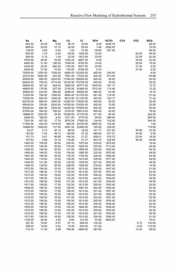
Reactive Flow Modeling of Hydrothermal Systems 253
Na K Mg Ca Cl SO4 HCO3 CO3 CO2 SIO2
922.00 34.00 9.50 28.70 30.00 0.45 2540.70 64.50
868.00 30.00 10.10 30.00 29.50 1.60 2556.00 70.50
128.00 3.60 0.03 1.00 37.80 38.80 207.40 86.00
850.00 1.70 0.60 39.00 1320.00 18.00 53.00 55.00
904.00 5.10 1.00 32.00 1423.00 20.00 22.00 42.00
4760.00 36.00 33.00 1435.00 9847.00 6.00 35.00 22.00
4840.00 31.00 106.00 1090.00 9750.00 14.00 29.00 15.00
2240.00 25.00 660.00 1745.00 8037.00 20.00 37.00 8.50
4460.00 27.00 70.00 755.00 8794.00 4.10 37.00 6.20
75000.00 1250.00 1300.00 6690.00 132200.00 465.00 240.00 6.00
33318.00 3264.00 442.00 7581.00 73323.00 220.00 473.00 63.98
85000.00 660.00 2520.00 17400.00 169000.00 400.00 35.00 20.00
88200.00 750.00 2710.00 18100.00 175700.00 500.00 35.00 20.00
48900.00 181.00 638.00 2080.00 80777.00 1000.00 181.17 12.72
48800.00 179.00 637.00 2150.00 81669.00 1010.00 174.46 12.25
48850.00 243.00 660.00 2080.00 80525.00 960.00 53.00 15.15
72300.00 792.00 1380.00 8840.00 131700.00 481.00 118.34 31.42
73000.00 864.00 1400.00 8612.00 131100.00 463.00 120.17 31.42
92700.00 680.00 2350.00 14350.00 175000.00 400.00 50.00 20.00
95000.00 700.00 2430.00 14700.00 179300.00 400.00 70.00 20.00
93000.00 690.00 2300.00 14450.00 175500.00 400.00 50.00 20.00
57650.00 264.00 780.00 2730.00 95615.00 900.00 40.00 16.92
18886.00 1200.00 24.50 10428.00 47100.00 411.00 60.00 242.00
2368.00 180.00 6.00 1271.00 5770.00 56.00 268.00 265.00
7261.00 497.00 17.70 3676.00 17650.00 134.00 102.00 344.00
11845.00 424.00 1419.00 465.00 20100.00 2865.00 144.00 1.80
10898.00 1089.00 131.00 2497.00 22800.00 145.00 238.00 179.00
62.07 3.13 30.14 88.00 19.50 151.77 331.00 30.80 23.30
152.65 7.04 48.13 128.80 27.30 490.90 331.01 44.00 5.30
151.73 5.47 46.68 144.00 21.27 658.01 278.75 22.00 19.00
167.83 4.69 33.74 116.80 21.27 543.70 326.66 44.00 20.80
1483.00 156.00 30.00 228.00 1675.00 229.00 1870.00 18.40
1472.00 156.00 29.00 176.00 1640.00 233.00 1712.00 26.00
1455.00 146.00 20.00 127.00 1595.00 233.00 1553.00 54.30
1455.00 146.00 16.00 134.00 1595.00 233.00 1553.00 48.60
1481.00 195.00 25.00 135.00 1702.00 226.00 1595.00 44.00
1504.00 116.00 15.00 136.00 1613.00 229.00 1577.00 49.00
1546.00 131.00 35.00 130.00 1764.00 227.00 1555.00 46.00
1380.00 135.00 48.00 228.00 1539.00 216.00 1897.00 15.00
1472.00 156.00 23.00 128.00 1613.00 248.00 1547.00 51.00
1471.00 156.00 17.00 133.00 1613.00 237.00 1551.00 52.50
1472.00 156.00 19.00 132.00 1613.00 248.00 1548.00 52.00
1471.00 156.00 16.00 132.00 1613.00 244.00 1549.00 50.50
1472.00 156.00 19.00 131.00 1613.00 241.00 1548.00 49.00
1471.00 156.00 17.00 132.00 1613.00 250.00 1550.00 50.50
1509.00 156.00 15.00 128.00 1667.00 242.00 1550.00 52.00
1472.00 156.00 17.00 148.00 1613.00 231.00 1597.00 53.00
1472.00 156.00 16.00 138.00 1613.00 231.00 1565.00 55.00
1472.00 156.00 16.00 131.00 1613.00 242.00 1567.00 53.50
1472.00 156.00 15.00 140.00 1613.00 249.00 1554.00 50.50
1472.00 156.00 18.00 128.00 1613.00 236.00 1546.00 53.00
1555.00 156.00 14.00 142.00 1684.00 255.00 1638.00 57.00
1472.00 156.00 15.00 140.00 1613.00 250.00 1554.00 52.50
1472.00 156.00 17.00 127.00 1613.00 247.00 1555.00 56.50
1472.00 156.00 16.00 138.00 1613.00 254.00 1568.00 51.00
1100.00 26.00 3.30 8.00 107.00 53.00 2684.00 70.61
387.50 19.60 0.07 67.10 658.50 122.50 6.70 133.60
386.00 19.00 0.02 74.00 634.00 121.00 8.00 133.00
715.70 17.30 3.68 759.40 2460.00 297.60 13.30 49.00
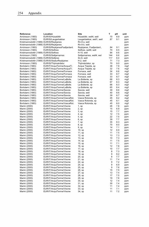
254 Appendix
Reference Location Site T pH unit
Arnórsson (1983) EUR/IS/Húsatóttir Húsatóttir, well4, well 70 8.9 ppm
Arnórsson (1983) EUR/IS/Laugarbakkar Laugarbakkar, well1, well 87 9.1 ppm
Kristmannsdottir (1989) EUR/IS/Reykjanes Rn-9 a, well ppm
Kristmannsdottir (1989) EUR/IS/Reykjanes Rn-9 b, well ppm
Arnórsson (1983) EUR/IS/ReykjanesFsafjardard. Reykjanes, Fsafjardard., 84 9.1 ppm
Arnórsson (1983) EUR/IS/Selfoss Selfoss, well9, well 70 8.5 ppm
Kristmannsdottir (1989) EUR/IS/Selfoss H-10, well 84 8.6 ppm
Arnórsson (1983) EUR/IS/Seltjarnarnes Seltjarnarnes, well4, wel 144 8.6 ppm
Kristmannsdottir (1989) EUR/IS/Seltjnes Sn-6, well 117 8.4 ppm
Kristmannsdottir (1989) EUR/IS/StadurReykjanes H-2, well 71 7.3 ppm
Arnórsson (1983) EUR/IS/Thjórsárdalur Thjórsárdalur, sp 70 9.0 ppm
Bortolami (1983) EUR/IT/AcquiTerme/AcquaTi. Acqua Tiepida, sp 38 7.9 mg/l
Bortolami (1983) EUR/IT/AcquiTerme/AcquaTi. Acqua Tiepida, sp 32 7.6 mg/l
Bortolami (1983) EUR/IT/AcquiTerme/Fornace Fornace, well 34 8.6 mg/l
Bortolami (1983) EUR/IT/AcquiTerme/Fornace Fornace, well 33 8.7 mg/l
Bortolami (1983) EUR/IT/AcquiTerme/Fornace Fornace, well 33 8.7 mg/l
Bortolami (1983) EUR/IT/AcquiTerme/LaBolle. La Bollente, sp 68 8.3 mg/l
Bortolami (1983) EUR/IT/AcquiTerme/LaBolle. La Bollente, sp 67 8.3 mg/l
Bortolami (1983) EUR/IT/AcquiTerme/LaBolle. La Bollente, sp 66 8.3 mg/l
Bortolami (1983) EUR/IT/AcquiTerme/LaBolle. La Bollente, sp 65 8.4 mg/l
Bortolami (1983) EUR/IT/AcquiTerme/Savoia Savoia, well 39 8.6 mg/l
Bortolami (1983) EUR/IT/AcquiTerme/Savoia Savoia, well 40 8.6 mg/l
Bortolami (1983) EUR/IT/AcquiTerme/Savoia Savoia, well 39 8.7 mg/l
Bortolami (1983) EUR/IT/AcquiTerme/VascaRot. Vasca Rotonda, sp 45 8.2 mg/l
Bortolami (1983) EUR/IT/AcquiTerme/VascaRot. Vasca Rotonda, sp 45 8.1 mg/l
Bortolami (1983) EUR/IT/AcquiTerme/VascaRot. Vasca Rotonda, sp 45 8.0 mg/l
Marini (2000) EUR/IT/AcquiTerme/Visone 1, sp 26 7.8 ppm
Marini (2000) EUR/IT/AcquiTerme/Visone 2, sp 15 6.9 ppm
Marini (2000) EUR/IT/AcquiTerme/Visone 3, sp 15 7.7 ppm
Marini (2000) EUR/IT/AcquiTerme/Visone 4, sp 12 7.5 ppm
Marini (2000) EUR/IT/AcquiTerme/Visone 5, sp 22 7.5 ppm
Marini (2000) EUR/IT/AcquiTerme/Visone 6, sp 39 7.7 ppm
Marini (2000) EUR/IT/AcquiTerme/Visone 7, sp 35 8.3 ppm
Marini (2000) EUR/IT/AcquiTerme/Visone 8, sp 70 8.0 ppm
Marini (2000) EUR/IT/AcquiTerme/Visone 9, sp 14 7.1 ppm
Marini (2000) EUR/IT/AcquiTerme/Visone 10, sp 12 6.9 ppm
Marini (2000) EUR/IT/AcquiTerme/Visone 11, sp 11 7.5 ppm
Marini (2000) EUR/IT/AcquiTerme/Visone 12, sp 13 7.3 ppm
Marini (2000) EUR/IT/AcquiTerme/Visone 13, sp 10 7.3 ppm
Marini (2000) EUR/IT/AcquiTerme/Visone 14, sp 11 7.5 ppm
Marini (2000) EUR/IT/AcquiTerme/Visone 15, sp 11 7.1 ppm
Marini (2000) EUR/IT/AcquiTerme/Visone 16, sp 12 7.8 ppm
Marini (2000) EUR/IT/AcquiTerme/Visone 17, sp 10 7.7 ppm
Marini (2000) EUR/IT/AcquiTerme/Visone 18, sp 8 7.3 ppm
Marini (2000) EUR/IT/AcquiTerme/Visone 19, sp 9 8.2 ppm
Marini (2000) EUR/IT/AcquiTerme/Visone 20, sp 8 7.7 ppm
Marini (2000) EUR/IT/AcquiTerme/Visone 21, sp 11 7.4 ppm
Marini (2000) EUR/IT/AcquiTerme/Visone 22, sp 9 7.2 ppm
Marini (2000) EUR/IT/AcquiTerme/Visone 24, sp 9 6.9 ppm
Marini (2000) EUR/IT/AcquiTerme/Visone 25, sp 9 7.6 ppm
Marini (2000) EUR/IT/AcquiTerme/Visone 26, sp 15 7.5 ppm
Marini (2000) EUR/IT/AcquiTerme/Visone 27, sp 13 7.4 ppm
Marini (2000) EUR/IT/AcquiTerme/Visone 28, sp 17 7.5 ppm
Marini (2000) EUR/IT/AcquiTerme/Visone 29, sp 19 7.6 ppm
Marini (2000) EUR/IT/AcquiTerme/Visone 30, sp 12 7.4 ppm
Marini (2000) EUR/IT/AcquiTerme/Visone 31, sp 30 7.4 ppm
Marini (2000) EUR/IT/AcquiTerme/Visone 32, sp 11 7.4 ppm
Marini (2000) EUR/IT/AcquiTerme/Visone 33, sp 11 7.1 ppm
Marini (2000) EUR/IT/AcquiTerme/Visone 34, sp 11 7.2 ppm
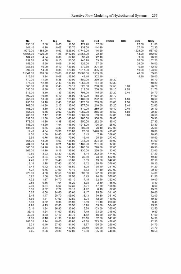
Reactive Flow Modeling of Hydrothermal Systems 255
Na K Mg Ca Cl SO4 HCO3 CO3 CO2 SIO2
136.10 2.88 0.05 11.30 171.70 67.60 22.00 71.80
141.40 4.20 0.07 23.70 139.50 144.90 27.40 102.30
9079.00 1388.00 0.93 1526.00 17749.00 16.20 1523.00 587.00
12564.00 1920.00 1.28 2112.00 24558.00 22.40 14.20 812.00
184.20 4.34 0.09 67.60 390.20 42.10 9.00 70.90
159.60 4.58 0.15 30.30 246.70 53.50 26.00 62.20
158.00 5.60 0.09 24.00 226.00 57.00 24.00 76.00
355.50 10.00 0.10 139.00 670.80 204.80 6.50 112.10
597.00 14.00 0.38 523.00 1617.00 305.00 10.00 123.00
11041.00 399.00 109.00 1915.00 19880.00 1535.00 40.00 69.00
115.60 3.24 0.08 52.90 49.40 302.30 5.90 58.00
770.00 11.90 5.35 130.00 1180.00 270.00 29.30 56.70
675.00 12.40 2.43 137.00 1066.00 184.00 43.30 48.80
565.00 8.80 2.43 76.10 826.00 208.00 27.50 3.60 26.20
555.00 8.80 1.95 78.50 812.00 200.00 28.10 4.20 31.70
513.00 8.10 1.33 80.90 794.00 145.00 23.20 2.40 28.70
700.00 16.30 6.10 136.00 1170.00 188.00 39.70 54.00
765.00 13.20 4.86 128.00 1180.00 292.00 39.70 1.50 48.60
755.00 14.10 2.43 135.00 1175.00 285.00 33.60 1.50 59.30
768.00 14.30 2.13 135.00 1177.00 210.00 23.20 2.40 52.60
755.00 8.60 3.40 120.00 1110.00 289.00 49.40 2.40 25.10
651.00 6.56 2.92 122.00 1060.00 255.00 19.50 1.80 29.30
700.00 7.17 2.31 126.00 1069.00 189.00 34.80 3.60 26.50
832.00 11.80 3.65 140.00 1260.00 306.00 59.80 50.90
778.00 14.30 4.38 143.00 1250.00 262.00 35.40 57.30
785.00 13.50 1.94 146.00 1213.00 196.00 25.60 53.30
435.00 6.75 4.87 35.20 609.00 76.10 257.00 25.60
19.40 4.64 65.30 623.00 26.30 1420.00 425.00 18.80
11.50 1.00 24.40 42.50 5.45 7.99 269.00 28.90
9.55 0.76 19.20 70.90 16.40 25.20 277.00 15.60
561.00 13.00 4.03 135.00 948.00 204.00 89.00 44.00
704.00 14.80 0.21 142.00 1160.00 231.00 17.00 52.30
685.00 14.70 0.54 140.00 1180.00 228.00 27.00 48.90
665.00 14.10 0.16 135.00 1130.00 230.00 23.00 52.60
12.50 3.93 63.30 132.00 8.14 222.00 474.00 37.20
12.70 3.04 27.00 175.00 30.50 73.20 502.00 19.40
4.48 1.82 35.40 59.80 3.89 19.20 342.00 12.10
8.16 1.18 37.40 93.30 8.12 88.70 378.00 18.10
3.41 0.42 33.40 68.60 5.05 35.40 331.00 14.20
4.22 0.56 27.90 77.10 5.63 67.10 297.00 20.40
229.00 4.50 12.50 102.00 390.00 122.00 233.00 24.80
6.22 1.06 68.50 32.50 6.45 74.80 370.00 41.30
4.72 1.17 34.70 63.10 7.15 32.50 322.00 10.00
2.55 0.36 1.04 18.20 3.78 2.19 56.00 8.40
2.90 0.84 5.67 52.30 8.01 17.30 168.00 8.60
6.06 0.82 2.27 26.10 4.92 8.19 87.00 15.20
5.65 0.58 24.60 95.60 4.17 95.50 311.00 26.60
5.45 1.47 20.70 109.00 6.13 70.80 361.00 12.00
4.66 1.31 17.60 12.60 5.04 12.20 119.00 19.30
5.08 0.52 9.36 85.90 5.89 31.40 260.00 9.40
19.90 4.15 42.80 58.50 10.90 65.00 364.00 15.50
5.10 1.84 26.80 110.00 5.28 103.00 365.00 12.50
35.10 4.54 11.60 87.50 7.49 73.00 315.00 9.90
40.30 3.33 37.10 49.70 4.52 46.50 391.00 17.60
11.00 6.16 21.90 119.00 28.10 82.70 341.00 14.30
188.00 5.14 40.00 46.80 47.80 273.00 476.00 22.50
3.31 0.40 27.40 91.00 3.77 135.00 255.00 24.70
27.90 2.34 49.50 143.00 36.40 176.00 469.00 24.70
7.45 2.96 29.30 132.00 12.50 65.00 440.00 16.50
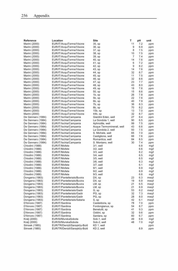
256 Appendix
Reference Location Site T pH unit
Marini (2000) EUR/IT/AcquiTerme/Visone 35, sp 11 7.2 ppm
Marini (2000) EUR/IT/AcquiTerme/Visone 36, sp 9 6.9 ppm
Marini (2000) EUR/IT/AcquiTerme/Visone 37, sp 8 7.5 ppm
Marini (2000) EUR/IT/AcquiTerme/Visone 38, sp 10 7.5 ppm
Marini (2000) EUR/IT/AcquiTerme/Visone 39, sp 7 7.4 ppm
Marini (2000) EUR/IT/AcquiTerme/Visone 40, sp 14 7.6 ppm
Marini (2000) EUR/IT/AcquiTerme/Visone 41, sp 6 7.2 ppm
Marini (2000) EUR/IT/AcquiTerme/Visone 42, sp 9 8.2 ppm
Marini (2000) EUR/IT/AcquiTerme/Visone 43, sp 14 7.6 ppm
Marini (2000) EUR/IT/AcquiTerme/Visone 44, sp 32 8.7 ppm
Marini (2000) EUR/IT/AcquiTerme/Visone 45, sp 11 7.5 ppm
Marini (2000) EUR/IT/AcquiTerme/Visone 46, sp 32 8.6 ppm
Marini (2000) EUR/IT/AcquiTerme/Visone 47, sp 23 7.7 ppm
Marini (2000) EUR/IT/AcquiTerme/Visone 48, sp 43 8.0 ppm
Marini (2000) EUR/IT/AcquiTerme/Visone 49, sp 18 7.6 ppm
Marini (2000) EUR/IT/AcquiTerme/Visone 50, sp 15 8.6 ppm
Marini (2000) EUR/IT/AcquiTerme/Visone 1b, sp 26 7.8 ppm
Marini (2000) EUR/IT/AcquiTerme/Visone 5b, sp 22 7.6 ppm
Marini (2000) EUR/IT/AcquiTerme/Visone 6b, sp 40 7.9 ppm
Marini (2000) EUR/IT/AcquiTerme/Visone 7b, sp 36 8.3 ppm
Marini (2000) EUR/IT/AcquiTerme/Visone 8b, sp 70 8.2 ppm
Marini (2000) EUR/IT/AcquiTerme/Visone 15b, sp 13 7.0 ppm
Marini (2000) EUR/IT/AcquiTerme/Visone 44b, sp 32 8.7 ppm
De Gennaro (1984) EUR/IT/Ischia/Campania Giardini Eden, well 27 6.4 ppm
De Gennaro (1984) EUR/IT/Ischia/Campania La Gondola 1, well 90 6.5 ppm
De Gennaro (1984) EUR/IT/Ischia/Campania Aphrodite, well 99 7.5 ppm
De Gennaro (1984) EUR/IT/Ischia/Campania Acque Termominerali, well 43 6.6 ppm
De Gennaro (1984) EUR/IT/Ischia/Campania La Gondola 2, well 93 7.5 ppm
De Gennaro (1984) EUR/IT/Ischia/Campania S. Michele, well 65 7.0 ppm
De Gennaro (1984) EUR/IT/Ischia/Campania Castiglione, well 66 7.6 ppm
De Gennaro (1984) EUR/IT/Ischia/Campania Romantica, well 84 8.5 ppm
De Gennaro (1984) EUR/IT/Ischia/Campania S. Montano, well 30 7.4 ppm
Chiodini (1988) EUR/IT/Mofete 3/1, well 6.8 mg/l
Chiodini (1988) EUR/IT/Mofete 3/2, well 6.6 mg/l
Chiodini (1988) EUR/IT/Mofete 3/3, well 6.2 mg/l
Chiodini (1988) EUR/IT/Mofete 3/4, well 6.5 mg/l
Chiodini (1988) EUR/IT/Mofete 3/5, well 6.5 mg/l
Chiodini (1988) EUR/IT/Mofete 3/6, well 6.3 mg/l
Chiodini (1988) EUR/IT/Mofete 3/7, well 6.1 mg/l
Chiodini (1988) EUR/IT/Mofete 9/1, well 6.9 mg/l
Chiodini (1988) EUR/IT/Mofete 9/2, well 6.9 mg/l
Chiodini (1988) EUR/IT/Mofete 9/3, well 6.6 mg/l
Dongarra (1983) EUR/IT/PantelleriaIs/Buvira DX, sp 23 6.3 meq/l
Dongarra (1983) EUR/IT/PantelleriaIs/Buvira DX, sp 19 6.9 meq/l
Dongarra (1983) EUR/IT/PantelleriaIs/Buvira LM, sp 21 6.5 meq/l
Dongarra (1983) EUR/IT/PantelleriaIs/Buvira LM, sp 21 6.9 meq/l
Dongarra (1983) EUR/IT/PantelleriaIs/Gadir G, sp 53 6.2 meq/l
Dongarra (1983) EUR/IT/PantelleriaIs/Gadir PG, sp 32 7.3 meq/l
Dongarra (1983) EUR/IT/PantelleriaIs/Gadir PG, sp 28 8.0 meq/l
Dongarra (1983) EUR/IT/PantelleriaIs/Sataria S, sp 42 6.1 meq/l
D'Amore (1987) EUR/IT/Sardinia Casteldoria, sp 78 7.0 ppm
D'Amore (1987) EUR/IT/Sardinia Fordongianus, sp 54 8.7 ppm
D'Amore (1987) EUR/IT/Sardinia Benetutti, sp 41 9.3 ppm
D'Amore (1987) EUR/IT/Sardinia Oddini, sp 32 9.6 ppm
D'Amore (1987) EUR/IT/Sardinia Sardara, sp 60 6.7 ppm
Kralj (2000) EUR/SI/MurskaSobota Sob-1, well 49 6.9 mg/l
Kralj (2000) EUR/SI/MurskaSobota Sob-2, well 48 7.0 mg/l
Simsek (1985) EUR/TR/Denizli/Sarayköy-Buld KD 1, well ppm
Simsek (1985) EUR/TR/Denizli/Sarayköy-Buld KD 2, well 8.9 ppm
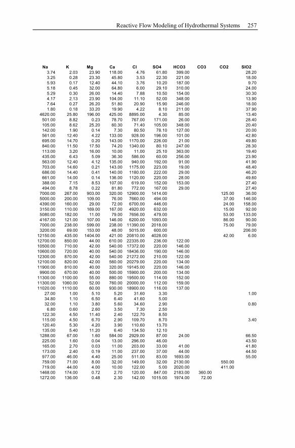
Reactive Flow Modeling of Hydrothermal Systems 257
Na K Mg Ca Cl SO4 HCO3 CO3 CO2 SIO2
3.74 2.03 23.90 118.00 4.76 61.80 399.00 28.20
3.25 0.28 23.30 45.80 3.53 22.30 221.00 18.00
5.93 0.17 12.40 44.10 3.76 10.20 187.00 9.70
5.18 0.45 32.00 64.80 6.00 29.10 310.00 24.00
5.29 0.30 26.00 14.40 7.88 10.50 154.00 30.30
4.17 2.13 23.90 104.00 11.10 52.00 348.00 13.90
7.64 0.27 26.20 51.80 20.90 15.90 246.00 18.00
1.80 0.18 33.20 19.90 4.22 8.10 211.00 37.90
4620.00 25.80 196.00 425.00 8895.00 4.30 85.00 13.40
501.00 8.82 0.23 78.70 767.00 171.00 26.00 28.40
105.00 8.62 25.20 60.30 71.40 105.00 348.00 20.40
142.00 1.90 0.14 7.30 80.50 78.10 127.00 20.00
561.00 12.40 4.22 133.00 928.00 196.00 101.00 42.80
695.00 14.70 0.20 143.00 1170.00 226.00 21.00 49.80
840.00 11.50 17.50 74.20 1340.00 80.10 247.00 28.30
113.00 3.20 16.00 10.00 11.00 25.10 363.00 19.40
435.00 6.43 5.09 36.30 586.00 60.00 256.00 23.90
563.00 12.40 4.12 135.00 940.00 192.00 91.00 41.90
703.00 14.60 0.21 143.00 1175.00 223.00 19.00 48.40
686.00 14.40 0.41 140.00 1180.00 222.00 29.00 46.20
661.00 14.00 0.14 136.00 1120.00 220.00 28.00 49.60
388.00 7.15 8.53 107.00 619.00 152.00 153.00 27.40
494.00 8.78 0.22 81.80 772.00 167.00 29.00 27.40
7000.00 267.00 903.00 320.00 12900.00 1414.00 125.00 36.00
5000.00 200.00 109.00 76.00 7660.00 494.00 37.00 146.00
4390.00 160.00 29.00 72.00 6700.00 446.00 24.00 158.00
3150.00 110.00 169.00 167.00 4920.00 632.00 15.00 92.00
5080.00 182.00 11.00 79.00 7656.00 479.00 53.00 133.00
4167.00 121.00 107.00 146.00 6200.00 1093.00 86.00 90.00
7000.00 238.00 599.00 238.00 11390.00 2018.00 75.00 79.00
3200.00 69.00 153.00 48.00 5015.00 600.00 206.00
12150.00 435.00 1404.00 421.00 20810.00 4028.00 42.00 6.00
12700.00 850.00 44.00 610.00 22335.00 236.00 122.00
10500.00 710.00 42.00 540.00 17372.00 220.00 146.00
10600.00 720.00 40.00 540.00 18436.00 190.00 146.00
12300.00 870.00 42.00 540.00 21272.00 210.00 122.00
12100.00 820.00 42.00 560.00 20279.00 220.00 134.00
11900.00 810.00 40.00 320.00 19145.00 220.00 146.00
9900.00 670.00 40.00 500.00 15900.00 200.00 134.00
11300.00 1100.00 55.00 880.00 19500.00 114.00 152.00
11300.00 1060.00 52.00 760.00 20000.00 112.00 159.00
11020.00 1110.00 60.00 930.00 18900.00 116.00 137.00
27.00 1.00 5.10 5.20 31.60 3.30 1.00
34.80 1.10 6.50 6.40 41.60 5.00
32.00 1.10 3.80 5.60 34.60 2.90 0.80
6.80 0.60 2.60 3.50 7.30 2.50
122.30 4.50 11.40 2.40 122.70 8.50
115.00 4.50 6.70 2.90 109.70 8.70 3.40
120.40 5.30 4.20 3.90 110.60 13.70
135.00 5.40 11.20 6.40 134.50 12.10
1288.00 67.00 1.60 584.00 2929.00 87.00 24.00 66.50
225.00 1.60 0.04 13.00 296.00 46.00 43.50
165.00 2.70 0.03 11.00 203.00 33.00 41.00 41.80
173.00 2.40 0.19 11.00 237.00 37.00 44.00 44.50
977.00 46.00 4.40 25.00 511.00 83.00 1693.00 55.00
759.00 71.00 8.00 32.00 149.00 32.00 2130.00 550.00
719.00 44.00 4.00 10.00 122.00 5.00 2020.00 411.00
1468.00 174.00 0.72 2.70 120.00 847.00 2183.00 360.00
1272.00 136.00 0.48 2.30 142.00 1015.00 1974.00 72.00
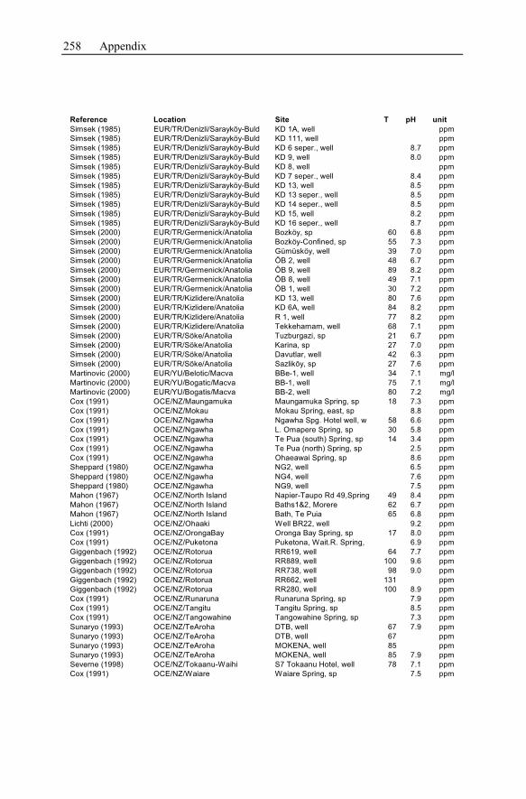
258 Appendix
Reference Location Site T pH unit
Simsek (1985) EUR/TR/Denizli/Sarayköy-Buld KD 1A, well ppm
Simsek (1985) EUR/TR/Denizli/Sarayköy-Buld KD 111, well ppm
Simsek (1985) EUR/TR/Denizli/Sarayköy-Buld KD 6 seper., well 8.7 ppm
Simsek (1985) EUR/TR/Denizli/Sarayköy-Buld KD 9, well 8.0 ppm
Simsek (1985) EUR/TR/Denizli/Sarayköy-Buld KD 8, well ppm
Simsek (1985) EUR/TR/Denizli/Sarayköy-Buld KD 7 seper., well 8.4 ppm
Simsek (1985) EUR/TR/Denizli/Sarayköy-Buld KD 13, well 8.5 ppm
Simsek (1985) EUR/TR/Denizli/Sarayköy-Buld KD 13 seper., well 8.5 ppm
Simsek (1985) EUR/TR/Denizli/Sarayköy-Buld KD 14 seper., well 8.5 ppm
Simsek (1985) EUR/TR/Denizli/Sarayköy-Buld KD 15, well 8.2 ppm
Simsek (1985) EUR/TR/Denizli/Sarayköy-Buld KD 16 seper., well 8.7 ppm
Simsek (2000) EUR/TR/Germenick/Anatolia Bozköy, sp 60 6.8 ppm
Simsek (2000) EUR/TR/Germenick/Anatolia Bozköy-Confined, sp 55 7.3 ppm
Simsek (2000) EUR/TR/Germenick/Anatolia Gümüsköy, well 39 7.0 ppm
Simsek (2000) EUR/TR/Germenick/Anatolia ÖB 2, well 48 6.7 ppm
Simsek (2000) EUR/TR/Germenick/Anatolia ÖB 9, well 89 8.2 ppm
Simsek (2000) EUR/TR/Germenick/Anatolia ÖB 8, well 49 7.1 ppm
Simsek (2000) EUR/TR/Germenick/Anatolia ÖB 1, well 30 7.2 ppm
Simsek (2000) EUR/TR/Kizlidere/Anatolia KD 13, well 80 7.6 ppm
Simsek (2000) EUR/TR/Kizlidere/Anatolia KD 6A, well 84 8.2 ppm
Simsek (2000) EUR/TR/Kizlidere/Anatolia R 1, well 77 8.2 ppm
Simsek (2000) EUR/TR/Kizlidere/Anatolia Tekkehamam, well 68 7.1 ppm
Simsek (2000) EUR/TR/Söke/Anatolia Tuzburgazi, sp 21 6.7 ppm
Simsek (2000) EUR/TR/Söke/Anatolia Karina, sp 27 7.0 ppm
Simsek (2000) EUR/TR/Söke/Anatolia Davutlar, well 42 6.3 ppm
Simsek (2000) EUR/TR/Söke/Anatolia Sazliköy, sp 27 7.6 ppm
Martinovic (2000) EUR/YU/Belotic/Macva BBe-1, well 34 7.1 mg/l
Martinovic (2000) EUR/YU/Bogatic/Macva BB-1, well 75 7.1 mg/l
Martinovic (2000) EUR/YU/Bogatis/Macva BB-2, well 80 7.2 mg/l
Cox (1991) OCE/NZ/Maungamuka Maungamuka Spring, sp 18 7.3 ppm
Cox (1991) OCE/NZ/Mokau Mokau Spring, east, sp 8.8 ppm
Cox (1991) OCE/NZ/Ngawha Ngawha Spg. Hotel well, w 58 6.6 ppm
Cox (1991) OCE/NZ/Ngawha L. Omapere Spring, sp 30 5.8 ppm
Cox (1991) OCE/NZ/Ngawha Te Pua (south) Spring, sp 14 3.4 ppm
Cox (1991) OCE/NZ/Ngawha Te Pua (north) Spring, sp 2.5 ppm
Cox (1991) OCE/NZ/Ngawha Ohaeawai Spring, sp 8.6 ppm
Sheppard (1980) OCE/NZ/Ngawha NG2, well 6.5 ppm
Sheppard (1980) OCE/NZ/Ngawha NG4, well 7.6 ppm
Sheppard (1980) OCE/NZ/Ngawha NG9, well 7.5 ppm
Mahon (1967) OCE/NZ/North Island Napier-Taupo Rd 49,Spring 49 8.4 ppm
Mahon (1967) OCE/NZ/North Island Baths1&2, Morere 62 6.7 ppm
Mahon (1967) OCE/NZ/North Island Bath, Te Puia 65 6.8 ppm
Lichti (2000) OCE/NZ/Ohaaki Well BR22, well 9.2 ppm
Cox (1991) OCE/NZ/OrongaBay Oronga Bay Spring, sp 17 8.0 ppm
Cox (1991) OCE/NZ/Puketona Puketona, Wait.R. Spring, 6.9 ppm
Giggenbach (1992) OCE/NZ/Rotorua RR619, well 64 7.7 ppm
Giggenbach (1992) OCE/NZ/Rotorua RR889, well 100 9.6 ppm
Giggenbach (1992) OCE/NZ/Rotorua RR738, well 98 9.0 ppm
Giggenbach (1992) OCE/NZ/Rotorua RR662, well 131 ppm
Giggenbach (1992) OCE/NZ/Rotorua RR280, well 100 8.9 ppm
Cox (1991) OCE/NZ/Runaruna Runaruna Spring, sp 7.9 ppm
Cox (1991) OCE/NZ/Tangitu Tangitu Spring, sp 8.5 ppm
Cox (1991) OCE/NZ/Tangowahine Tangowahine Spring, sp 7.3 ppm
Sunaryo (1993) OCE/NZ/TeAroha DTB, well 67 7.9 ppm
Sunaryo (1993) OCE/NZ/TeAroha DTB, well 67 ppm
Sunaryo (1993) OCE/NZ/TeAroha MOKENA, well 85 ppm
Sunaryo (1993) OCE/NZ/TeAroha MOKENA, well 85 7.9 ppm
Severne (1998) OCE/NZ/Tokaanu-Waihi S7 Tokaanu Hotel, well 78 7.1 ppm
Cox (1991) OCE/NZ/Waiare Waiare Spring, sp 7.5 ppm
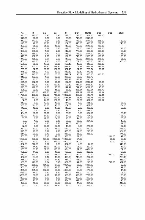
Reactive Flow Modeling of Hydrothermal Systems 259
Na K Mg Ca Cl SO4 HCO3 CO3 CO2 SIO2
1251.00 132.00 0.80 0.80 123.00 742.00 1906.00 361.00
1040.00 90.00 1.70 3.20 81.00 743.00 2043.00
1310.00 140.00 1.24 2.60 117.00 743.00 2147.00 258.00 120.00
1120.00 49.80 10.70 6.90 107.00 813.00 1426.00 261.00 248.00
1492.00 88.00 25.00 18.00 113.00 782.00 2147.00 453.00
1420.00 154.00 1.58 0.80 122.00 758.00 2147.00 318.00 125.00
1300.00 138.00 1.26 2.00 117.00 773.00 1880.00 360.00 120.00
1300.00 136.00 1.10 1.00 116.00 745.00 2144.00 240.00 128.00
1410.00 152.00 2.70 1.70 122.00 749.00 2388.00 180.00 128.00
1340.00 138.00 0.97 2.00 117.00 730.00 2257.00 216.00 125.00
1400.00 146.00 2.70 1.60 123.00 707.00 2385.00 198.00 360.00
1505.00 90.00 17.50 90.00 1152.12 46.30 1818.59 285.99
1320.00 100.00 67.50 167.50 1063.50 3.66 1611.13 489.12
705.00 62.50 30.00 152.50 957.15 37.50 729.74 56.07
1445.00 135.00 1.00 30.00 1559.80 33.30 1419.53
1440.00 140.00 10.00 85.00 1542.07 43.62 860.80 336.50
1410.00 122.50 1.50 62.50 1488.90 96.02 1396.72
1440.00 60.00 1.00 50.00 1595.25 125.85 1140.21
1125.00 132.50 1.00 20.00 102.80 637.03 2214.48 19.56
955.00 132.50 1.50 122.50 102.80 617.91 2055.30 32.60
1595.00 127.50 1.50 25.00 147.12 747.95 3222.20 45.66
905.00 92.50 4.50 45.00 88.62 988.84 820.94 218.70
9230.00 360.00 437.50 640.00 15598.00 1577.87 267.97 39.24
11725.00 480.00 462.50 715.00 19852.00 1858.98 119.74 22.44
1650.00 110.00 80.00 462.50 2747.37 58.73 1185.78 112.14
37.30 7.00 44.00 152.00 49.63 22.59 437.86 112.14
210.00 9.00 12.00 40.00 114.00 6.00 555.00 23.00
155.00 11.00 10.00 40.00 107.00 4.00 409.00 64.00
149.00 10.00 9.00 47.00 113.00 2.00 408.00 66.00
201.00 0.60 94.00 5.90 15.00 9.00 1039.00
434.00 60.90 80.30 8.50 73.00 9.00 1584.00 28.00
131.00 10.00 37.20 94.00 67.00 48.00 704.00 128.00
55.00 8.00 12.80 34.00 26.00 14.00 283.00 130.00
9.00 1.00 2.50 2.80 23.00 36.00 224.00 10.00
6.20 4.00 1.70 3.20 17.00 390.00 37.00
37.80 3.30 27.00 22.80 14.00 3.00 274.00 97.00
861.00 80.00 0.60 16.00 1162.00 42.00 590.00 426.00
1025.00 90.00 0.11 2.90 1475.00 27.00 298.00 464.00
1011.00 90.00 0.10 2.90 1437.00 35.00 486.00 471.00
500.00 9.00 0.10 12.00 660.00 82.00 111.00 42.00
6100.00 100.00 137.00 3900.00 16000.00 21.00 25.00 28.00
4550.00 22.00 8.00 815.00 8300.00 110.00 60.00 52.00
1007.00 217.00 0.01 1.30 1657.00 4.00 44.00 849.00
486.00 14.80 58.00 152.00 903.00 98.00 220.00 37.00
2000.00 80.70 57.00 195.00 1371.00 22.00 4471.00 62.00
185.00 14.00 0.20 10.00 159.00 33.00 228.00 157.00
1190.00 145.00 0.03 19.00 1865.00 11.00 50.00 630.00 448.00
452.00 34.00 0.12 13.00 393.00 219.00 287.00 263.00
318.00 77.00 0.13 11.60 387.00 148.00 121.00 283.00
933.00 126.00 0.04 3.10 1369.00 12.00 210.00 719.00 322.00
8474.00 238.00 181.00 37.90 9961.00 55.00 5937.00 22.00
453.00 40.80 63.00 42.70 19.00 11.00 1534.00 117.00
4365.00 305.00 162.00 99.00 5699.00 69.00 4170.00 14.00
3159.00 74.00 3.50 5.60 631.00 348.00 7700.00 108.00
3200.00 66.00 4.00 11.20 550.00 390.00 7700.00 133.00
3200.00 66.00 3.90 6.90 550.00 390.00 7500.00 135.00
3385.00 70.00 3.60 8.20 574.00 312.00 7500.00 116.00
436.00 48.00 36.60 53.00 685.00 14.00 281.00 216.00
56.00 3.50 55.50 49.80 35.00 7.00 556.00 80.00
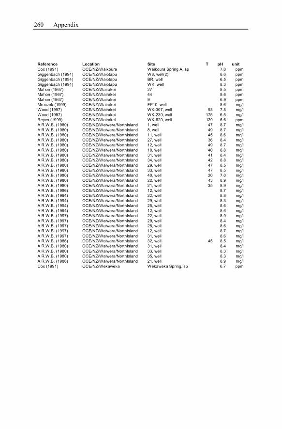
260 Appendix
Reference Location Site T pH unit
Cox (1991) OCE/NZ/Waikoura Waikoura Spring A, sp 7.0 ppm
Giggenbach (1994) OCE/NZ/Waiotapu W8, well(2) 8.6 ppm
Giggenbach (1994) OCE/NZ/Waiotapu BR, well 6.5 ppm
Giggenbach (1994) OCE/NZ/Waiotapu WK, well 8.3 ppm
Mahon (1967) OCE/NZ/Wairakei 27 8.5 ppm
Mahon (1967) OCE/NZ/Wairakei 44 8.6 ppm
Mahon (1967) OCE/NZ/Wairakei 9 6.9 ppm
Mroczek (1999) OCE/NZ/Wairakei FP10, well 8.6 mg/l
Wood (1997) OCE/NZ/Wairakei WK-307, well 93 7.8 mg/l
Wood (1997) OCE/NZ/Wairakei WK-230, well 175 6.5 mg/l
Reyes (1999) OCE/NZ/Wairakei WK-620, well 129 6.6 ppm
A.R.W.B. (1980) OCE/NZ/Waiwera/NorthIsland 1, well 47 8.7 mg/l
A.R.W.B. (1980) OCE/NZ/Waiwera/NorthIsland 8, well 49 8.7 mg/l
A.R.W.B. (1980) OCE/NZ/Waiwera/NorthIsland 11, well 45 8.6 mg/l
A.R.W.B. (1980) OCE/NZ/Waiwera/NorthIsland 27, well 36 8.4 mg/l
A.R.W.B. (1980) OCE/NZ/Waiwera/NorthIsland 12, well 49 8.7 mg/l
A.R.W.B. (1980) OCE/NZ/Waiwera/NorthIsland 18, well 40 8.8 mg/l
A.R.W.B. (1980) OCE/NZ/Waiwera/NorthIsland 31, well 41 8.4 mg/l
A.R.W.B. (1980) OCE/NZ/Waiwera/NorthIsland 34, well 42 8.8 mg/l
A.R.W.B. (1980) OCE/NZ/Waiwera/NorthIsland 29, well 47 8.5 mg/l
A.R.W.B. (1980) OCE/NZ/Waiwera/NorthIsland 33, well 47 8.5 mg/l
A.R.W.B. (1980) OCE/NZ/Waiwera/NorthIsland 40, well 20 7.0 mg/l
A.R.W.B. (1980) OCE/NZ/Waiwera/NorthIsland 22, well 43 8.9 mg/l
A.R.W.B. (1980) OCE/NZ/Waiwera/NorthIsland 21, well 35 8.9 mg/l
A.R.W.B. (1986) OCE/NZ/Waiwera/NorthIsland 12, well 8.7 mg/l
A.R.W.B. (1994) OCE/NZ/Waiwera/NorthIsland 22, well 8.8 mg/l
A.R.W.B. (1994) OCE/NZ/Waiwera/NorthIsland 29, well 8.3 mg/l
A.R.W.B. (1994) OCE/NZ/Waiwera/NorthIsland 25, well 8.6 mg/l
A.R.W.B. (1994) OCE/NZ/Waiwera/NorthIsland 12, well 8.6 mg/l
A.R.W.B. (1997) OCE/NZ/Waiwera/NorthIsland 22, well 8.9 mg/l
A.R.W.B. (1997) OCE/NZ/Waiwera/NorthIsland 29, well 8.4 mg/l
A.R.W.B. (1997) OCE/NZ/Waiwera/NorthIsland 25, well 8.6 mg/l
A.R.W.B. (1997) OCE/NZ/Waiwera/NorthIsland 12, well 8.7 mg/l
A.R.W.B. (1997) OCE/NZ/Waiwera/NorthIsland 31, well 8.6 mg/l
A.R.W.B. (1986) OCE/NZ/Waiwera/NorthIsland 32, well 45 8.5 mg/l
A.R.W.B. (1980) OCE/NZ/Waiwera/NorthIsland 31, well 8.4 mg/l
A.R.W.B. (1980) OCE/NZ/Waiwera/NorthIsland 33, well 8.3 mg/l
A.R.W.B. (1980) OCE/NZ/Waiwera/NorthIsland 35, well 8.3 mg/l
A.R.W.B. (1986) OCE/NZ/Waiwera/NorthIsland 21, well 8.9 mg/l
Cox (1991) OCE/NZ/Wekaweka Wekaweka Spring, sp 6.7 ppm
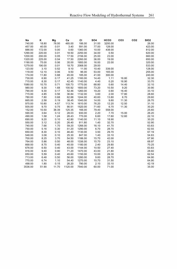
Reactive Flow Modeling of Hydrothermal Systems 261
Na K Mg Ca Cl SO4 HCO3 CO3 CO2 SIO2
740.00 18.80 78.00 465.00 186.00 31.00 3200.00 26.00
457.00 40.00 0.01 3.40 591.00 77.00 128.00 423.00
886.00 172.00 0.00 0.60 1360.00 10.00 438.00 812.00
1290.00 220.00 0.01 18.50 2250.00 34.00 0.50 620.00
1200.00 200.00 0.05 17.50 2156.00 25.00 23.00 660.00
1320.00 225.00 0.04 17.50 2260.00 36.00 19.00 650.00
1190.00 75.00 0.06 35.00 1950.00 16.00 22.00 320.00
1279.00 190.00 0.01 18.70 2068.00 29.00 533.00
123.00 3.10 0.52 9.10 11.00 10.40 339.00 128.00
118.00 12.10 0.06 9.50 96.00 53.00 165.00 255.00
174.00 11.80 0.88 45.00 185.00 41.00 300.00 240.00
730.00 6.90 0.17 41.25 1160.00 14.40 1.11 16.80 32.30
715.00 8.30 0.17 42.45 1140.00 4.40 0.20 16.90 33.70
1080.00 10.70 0.71 105.73 1770.00 68.80 0.60 14.40 32.10
980.00 9.30 1.68 100.92 1600.00 73.20 10.50 9.20 30.90
790.00 9.30 0.17 52.46 1260.00 19.20 0.60 16.40 33.10
715.00 4.85 0.56 36.84 1132.00 3.60 2.00 17.80 28.60
780.00 7.80 0.68 62.88 1244.00 40.60 13.80 6.70 29.60
665.00 2.58 0.19 38.45 1040.00 14.00 9.60 11.30 26.70
975.00 10.80 4.57 113.74 1610.00 76.20 12.20 12.50 31.10
935.00 9.70 0.75 90.51 1520.00 71.60 6.70 11.30 30.20
152.00 10.50 38.39 125.35 166.00 79.40 558.00 25.60
590.00 3.64 0.12 28.03 930.00 2.20 7.70 15.00 26.20
490.00 1.58 1.24 26.43 770.00 6.60 17.60 12.60 22.10
690.00 9.20 0.10 42.80 1140.00 11.10 18.90 30.20
550.00 3.12 0.20 26.40 911.80 1.40 32.70 52.90
740.00 7.66 1.70 59.20 1266.00 16.10 41.70 63.83
750.00 5.16 0.30 51.20 1290.00 6.70 28.70 62.55
650.00 8.30 0.10 46.40 1130.00 3.50 29.70 67.19
548.00 3.08 0.10 25.30 847.00 1.40 33.10 54.83
700.00 8.25 3.70 54.50 1186.00 15.70 42.00 67.90
764.00 5.86 0.50 48.00 1336.00 15.70 23.10 68.97
668.00 8.75 0.40 45.00 1180.00 2.40 29.80 70.25
676.00 6.50 0.40 43.00 1144.00 10.50 27.40 63.83
916.00 9.40 0.90 71.20 1470.00 43.00 21.80 28.60
650.00 5.59 0.40 45.60 1150.00 10.00 29.30 62.54
713.00 6.48 0.50 56.00 1280.00 9.60 28.70 64.90
770.00 6.74 1.10 54.40 1270.00 10.70 31.50 64.90
498.00 1.80 0.15 26.20 790.00 2.10 33.10 42.19
3536.00 51.90 11.70 1120.00 7540.00 60.00 71.00 35.00