Embed Size (px)
DESCRIPTION
Citation preview
Outline Introduction Chapter 2 Chapter 3 Chapter 4 Chapter 5 Chapter 6 Conclusions
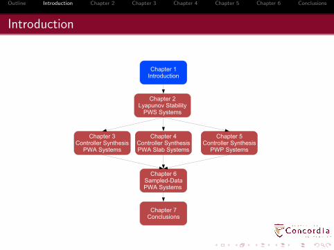
Stability Analysis and Controller Synthesis for a
Class of Piecewise Smooth Systems
The Oral Examinationfor the Degree of Doctor of Philosophy
Behzad Samadi
Department of Mechanical and Industrial EngineeringConcordia University
18 April 2008Montreal, Quebec
Canada
Outline Introduction Chapter 2 Chapter 3 Chapter 4 Chapter 5 Chapter 6 Conclusions
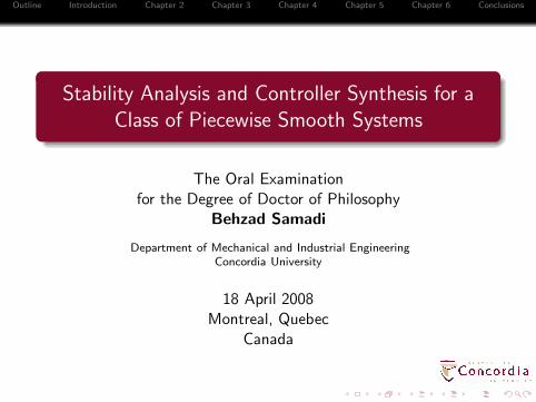
Outline
Outline Introduction Chapter 2 Chapter 3 Chapter 4 Chapter 5 Chapter 6 Conclusions
Introduction

Outline Introduction Chapter 2 Chapter 3 Chapter 4 Chapter 5 Chapter 6 Conclusions
Practical Motivation
c©Quanser
Memoryless Nonlinearities
Saturation Dead Zone Coulomb &Viscous Friction

Outline Introduction Chapter 2 Chapter 3 Chapter 4 Chapter 5 Chapter 6 Conclusions
Theoretical Motivation
Richard Murray, California Institute of Technology: “
Rank Top Ten Research Problems in Nonlinear Control
10 Building representative experiments for evaluating controllers
9 Convincing industry to invest in new nonlinear methodologies
8 Recognizing the difference between regulation and tracking
7 Exploiting special structure to analyze and design controllers
6 Integrating good linear techniques into nonlinear methodologies
5 Recognizing the difference between performance and operability
4 Finding nonlinear normal systems for control
3 Global robust stabilization and local robust performance
2 Magnitude and rate saturation
1 Writing numerical software for implementing nonlinear theory
...This is more or less a way for me to think online, so I wouldn’t take any of this
too seriously.”
Outline Introduction Chapter 2 Chapter 3 Chapter 4 Chapter 5 Chapter 6 Conclusions
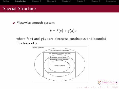
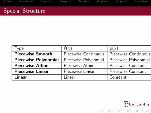
Special Structure
Piecewise smooth system:
x = f (x) + g(x)u
where f (x) and g(x) are piecewise continuous and boundedfunctions of x .
Outline Introduction Chapter 2 Chapter 3 Chapter 4 Chapter 5 Chapter 6 Conclusions
Objective
To develop a computational tool to design controllers forpiecewise smooth systems using convex optimization
techniques.
Outline Introduction Chapter 2 Chapter 3 Chapter 4 Chapter 5 Chapter 6 Conclusions
Objective
To develop a computational tool to design controllers forpiecewise smooth systems using convex optimization
techniques.
Why convex optimization?
There are numerically efficient tools to solve convexoptimization problems.Linear Matrix Inequalities (LMI)Sum of Squares (SOS) programming
Outline Introduction Chapter 2 Chapter 3 Chapter 4 Chapter 5 Chapter 6 Conclusions
Literature
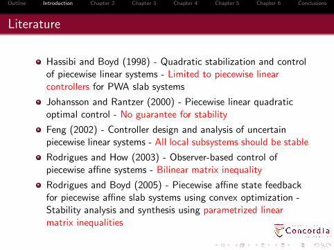
Hassibi and Boyd (1998) - Quadratic stabilization and controlof piecewise linear systems - Limited to piecewise linearcontrollers for PWA slab systems
Johansson and Rantzer (2000) - Piecewise linear quadraticoptimal control - No guarantee for stability
Feng (2002) - Controller design and analysis of uncertainpiecewise linear systems - All local subsystems should be stable
Rodrigues and How (2003) - Observer-based control ofpiecewise affine systems - Bilinear matrix inequality
Rodrigues and Boyd (2005) - Piecewise affine state feedbackfor piecewise affine slab systems using convex optimization -Stability analysis and synthesis using parametrized linearmatrix inequalities
Outline Introduction Chapter 2 Chapter 3 Chapter 4 Chapter 5 Chapter 6 Conclusions
Major Contributions
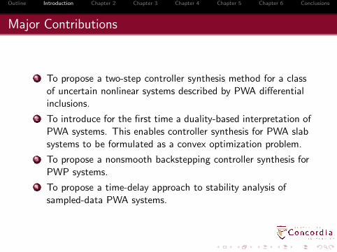
1 To propose a two-step controller synthesis method for a classof uncertain nonlinear systems described by PWA differentialinclusions.
2 To introduce for the first time a duality-based interpretation ofPWA systems. This enables controller synthesis for PWA slabsystems to be formulated as a convex optimization problem.
3 To propose a nonsmooth backstepping controller synthesis forPWP systems.
4 To propose a time-delay approach to stability analysis ofsampled-data PWA systems.
Outline Introduction Chapter 2 Chapter 3 Chapter 4 Chapter 5 Chapter 6 Conclusions
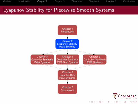
Lyapunov Stability for Piecewise Smooth Systems
Outline Introduction Chapter 2 Chapter 3 Chapter 4 Chapter 5 Chapter 6 Conclusions
Lyapunov Stability for Piecewise Smooth Systems
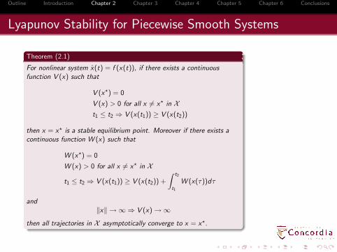
Theorem (2.1)
For nonlinear system x(t) = f (x(t)), if there exists a continuous
function V (x) such that
V (x⋆) = 0
V (x) > 0 for all x 6= x⋆ in X
t1 ≤ t2 ⇒ V (x(t1)) ≥ V (x(t2))
then x = x⋆ is a stable equilibrium point. Moreover if there exists a
continuous function W (x) such that
W (x⋆) = 0
W (x) > 0 for all x 6= x⋆ in X
t1 ≤ t2 ⇒ V (x(t1)) ≥ V (x(t2)) +
∫ t2
t1
W (x(τ))dτ
and
‖x‖ → ∞ ⇒ V (x) → ∞
then all trajectories in X asymptotically converge to x = x⋆.
Outline Introduction Chapter 2 Chapter 3 Chapter 4 Chapter 5 Chapter 6 Conclusions
Lyapunov Stability for Piecewise Smooth Systems
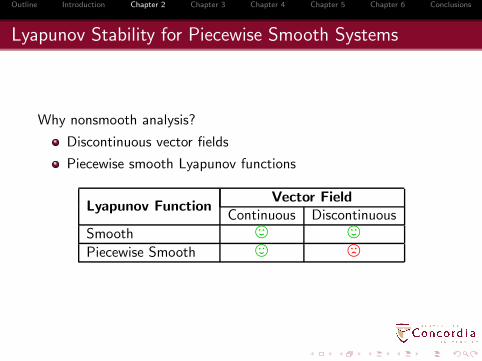
Why nonsmooth analysis?
Discontinuous vector fields
Piecewise smooth Lyapunov functions
Lyapunov FunctionVector Field
Continuous Discontinuous
Smooth , ,
Piecewise Smooth , /
Outline Introduction Chapter 2 Chapter 3 Chapter 4 Chapter 5 Chapter 6 Conclusions
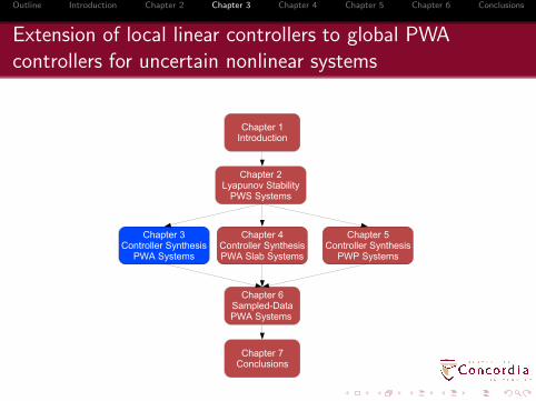
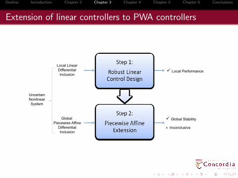
Extension of local linear controllers to global PWA
controllers for uncertain nonlinear systems
Outline Introduction Chapter 2 Chapter 3 Chapter 4 Chapter 5 Chapter 6 Conclusions
Extension of linear controllers to PWA controllers
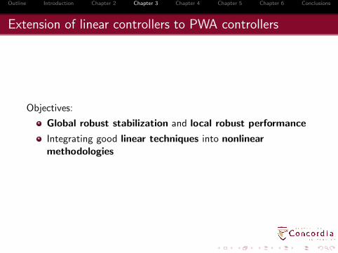
Objectives:
Global robust stabilization and local robust performance
Integrating good linear techniques into nonlinear
methodologies
Outline Introduction Chapter 2 Chapter 3 Chapter 4 Chapter 5 Chapter 6 Conclusions
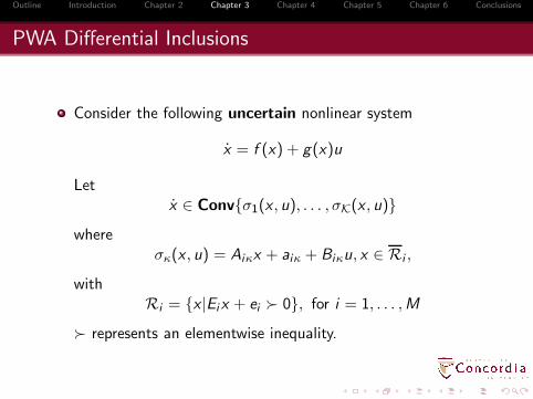
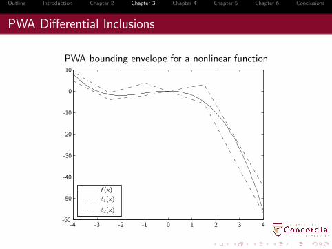
PWA Differential Inclusions
Consider the following uncertain nonlinear system
x = f (x) + g(x)u
Letx ∈ Convσ1(x , u), . . . , σK(x , u)
whereσκ(x , u) = Aiκx + aiκ + Biκu, x ∈ Ri ,
withRi = x |Eix + ei ≻ 0, for i = 1, . . . ,M
≻ represents an elementwise inequality.
Outline Introduction Chapter 2 Chapter 3 Chapter 4 Chapter 5 Chapter 6 Conclusions
PWA Differential Inclusions
PWA bounding envelope for a nonlinear function
f (x)
δ1(x)
δ2(x)
-4 -3 -2 -1 0 1 2 3 4-60
-50
-40
-30
-20
-10
0
10
Outline Introduction Chapter 2 Chapter 3 Chapter 4 Chapter 5 Chapter 6 Conclusions
Extension of linear controllers to PWA controllers

Outline Introduction Chapter 2 Chapter 3 Chapter 4 Chapter 5 Chapter 6 Conclusions
Extension of linear controllers to PWA controllers
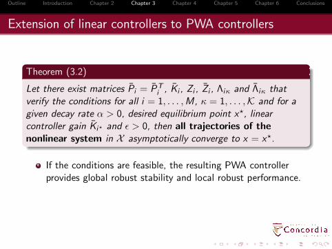
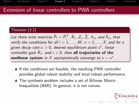
Theorem (3.2)
Let there exist matrices Pi = PTi , Ki , Zi , Zi , Λiκ and Λiκ that
verify the conditions for all i = 1, . . . ,M, κ = 1, . . . ,K and for a
given decay rate α > 0, desired equilibrium point x⋆, linear
controller gain Ki⋆ and ǫ > 0, then all trajectories of the
nonlinear system in X asymptotically converge to x = x⋆.
Outline Introduction Chapter 2 Chapter 3 Chapter 4 Chapter 5 Chapter 6 Conclusions
Extension of linear controllers to PWA controllers
Theorem (3.2)
Let there exist matrices Pi = PTi , Ki , Zi , Zi , Λiκ and Λiκ that
verify the conditions for all i = 1, . . . ,M, κ = 1, . . . ,K and for a
given decay rate α > 0, desired equilibrium point x⋆, linear
controller gain Ki⋆ and ǫ > 0, then all trajectories of the
nonlinear system in X asymptotically converge to x = x⋆.
If the conditions are feasible, the resulting PWA controllerprovides global robust stability and local robust performance.
The synthesis problem includes a set of Bilinear MatrixInequalities (BMI). In general, it is not convex.
Outline Introduction Chapter 2 Chapter 3 Chapter 4 Chapter 5 Chapter 6 Conclusions
Controller synthesis for PWA slab differential inclusions: a
duality-based convex optimization approach
Outline Introduction Chapter 2 Chapter 3 Chapter 4 Chapter 5 Chapter 6 Conclusions
Controller synthesis for PWA slab differential inclusions: a
duality-based convex optimization approach
Objective:
To formulate controller synthesis for stability and L2 gain
performance of piecewise affine slab differential inclusions asa set of LMIs.

Outline Introduction Chapter 2 Chapter 3 Chapter 4 Chapter 5 Chapter 6 Conclusions
L2 Gain Analysis for PWA Slab Differential Inclusions
PWA slab differential inclusion:
x ∈ConvAiκx + aiκ + Bwiκw , κ = 1, 2, (x ,w) ∈ RX×W
i
y ∈ConvCiκx + ciκ + Dwiκw , κ = 1, 2
RX×Wi =(x ,w)| ‖Lix + li + Miw‖ < 1
Parameter set:
Φ =
Aiκ1 aiκ1 Bwiκ1
Li li Mi
Ciκ2 ciκ2 Dwiκ2
∣
∣
∣
∣
∣
∣
i = 1, . . . ,M, κ1 = 1, 2, κ2 = 1, 2
Outline Introduction Chapter 2 Chapter 3 Chapter 4 Chapter 5 Chapter 6 Conclusions
A duality-based convex optimization approach
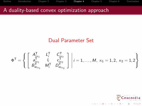
Dual Parameter Set
ΦT =
ATiκ1
LTi CT
iκ2
aTiκ1
li cTiκ2
BTwiκ1
MTi DT
wiκ2
∣
∣
∣
∣
∣
∣
i = 1, . . . ,M, κ1 = 1, 2, κ2 = 1, 2
Outline Introduction Chapter 2 Chapter 3 Chapter 4 Chapter 5 Chapter 6 Conclusions
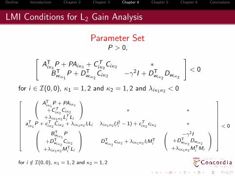
LMI Conditions for L2 Gain Analysis
Parameter SetP > 0,
[
ATiκ1
P + PAiκ1 + CTiκ2
Ciκ2 ∗BT
wiκ1P + DT
wiκ2Ciκ2 −γ2I + DT
wiκ2Dwiκ2
]
< 0
for i ∈ I(0, 0), κ1 = 1, 2 and κ2 = 1, 2 and λiκ1κ2 < 0
ATiκ1
P + PAiκ1
+CTiκ2
Ciκ2
+λiκ1κ2LT
i Li
∗ ∗
aTiκ1
P + cTiκ2
Ciκ2+ λiκ1κ2
liLi λiκ1κ2(l2i − 1) + cT
iκ2ciκ2
∗
BTwiκ1
P
+DTwiκ2
Ciκ2
+λiκ1κ2MT
i Li
DT
wiκ2ciκ2
+ λiκ1κ2liM
Ti
−γ2I+DT
wiκ2Dwiκ2
+λiκ1κ2MT
i Mi
< 0
for i /∈ I(0, 0), κ1 = 1, 2 and κ2 = 1, 2
Outline Introduction Chapter 2 Chapter 3 Chapter 4 Chapter 5 Chapter 6 Conclusions
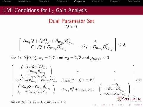
LMI Conditions for L2 Gain Analysis
Dual Parameter SetQ > 0,
[
Aiκ1Q + QATiκ1
+ Bwiκ1BT
wiκ1∗
Ciκ2Q + Dwiκ2BT
wiκ1−γ2I + Dwiκ2
DTwiκ2
]
< 0
for i ∈ I(0, 0), κ1 = 1, 2 and κ2 = 1, 2 and µiκ1κ2 < 0
Aiκ1Q + QAT
iκ1
+Bwiκ1BT
wiκ1
+µiκ1κ2aiκ1
aTiκ1
∗ ∗
LiQ + MiBTwiκ1
+ µiκ1κ2lia
Tiκ1
µiκ1κ2(l2i − 1) + MiM
Ti ∗
(
Ciκ2Q + Dwiκ2
BTwiκ1
+µiκ1κ2ciκ2
aTiκ1
)
Dwiκ2MT
i + µiκ1κ2liciκ2
−γ2I+Dwiκ2
DTwiκ2
+µiκ1κ2ciκ2
cTiκ2
< 0
for i /∈ I(0, 0), κ1 = 1, 2 and κ2 = 1, 2
Outline Introduction Chapter 2 Chapter 3 Chapter 4 Chapter 5 Chapter 6 Conclusions
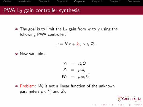
PWA L2 gain controller synthesis
The goal is to limit the L2 gain from w to y using thefollowing PWA controller:
u = Kix + ki , x ∈ Ri
New variables:
Yi = KiQ
Zi = µiki
Wi = µikikTi
Problem: Wi is not a linear function of the unknownparameters µi , Yi and Zi .
Outline Introduction Chapter 2 Chapter 3 Chapter 4 Chapter 5 Chapter 6 Conclusions
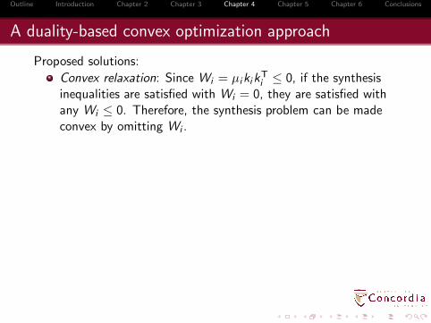
A duality-based convex optimization approach
Proposed solutions:
Convex relaxation: Since Wi = µikikTi ≤ 0, if the synthesis
inequalities are satisfied with Wi = 0, they are satisfied withany Wi ≤ 0. Therefore, the synthesis problem can be madeconvex by omitting Wi .
Outline Introduction Chapter 2 Chapter 3 Chapter 4 Chapter 5 Chapter 6 Conclusions
A duality-based convex optimization approach
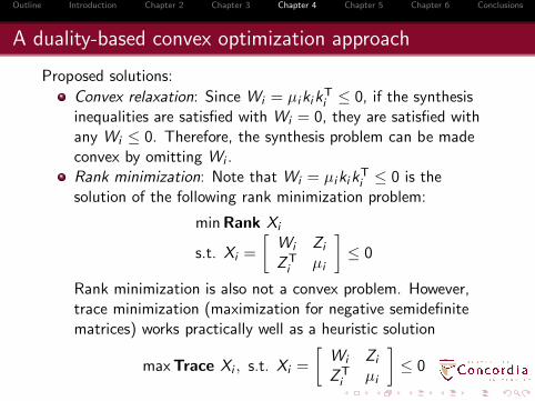
Proposed solutions:
Convex relaxation: Since Wi = µikikTi ≤ 0, if the synthesis
inequalities are satisfied with Wi = 0, they are satisfied withany Wi ≤ 0. Therefore, the synthesis problem can be madeconvex by omitting Wi .Rank minimization: Note that Wi = µikik
Ti ≤ 0 is the
solution of the following rank minimization problem:
min Rank Xi
s.t. Xi =
[
Wi Zi
ZTi µi
]
≤ 0
Rank minimization is also not a convex problem. However,trace minimization (maximization for negative semidefinitematrices) works practically well as a heuristic solution
maxTrace Xi , s.t. Xi =
[
Wi Zi
ZTi µi
]
≤ 0
Outline Introduction Chapter 2 Chapter 3 Chapter 4 Chapter 5 Chapter 6 Conclusions
A duality-based convex optimization approach
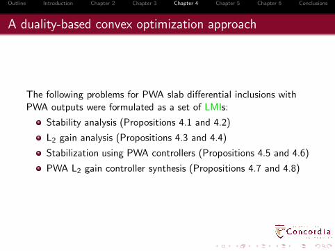
The following problems for PWA slab differential inclusions withPWA outputs were formulated as a set of LMIs:
Stability analysis (Propositions 4.1 and 4.2)
L2 gain analysis (Propositions 4.3 and 4.4)
Stabilization using PWA controllers (Propositions 4.5 and 4.6)
PWA L2 gain controller synthesis (Propositions 4.7 and 4.8)
Outline Introduction Chapter 2 Chapter 3 Chapter 4 Chapter 5 Chapter 6 Conclusions
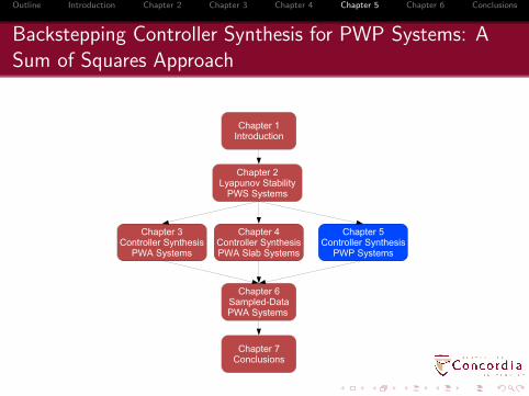
Backstepping Controller Synthesis for PWP Systems: A
Sum of Squares Approach
Outline Introduction Chapter 2 Chapter 3 Chapter 4 Chapter 5 Chapter 6 Conclusions
Backstepping Controller Synthesis for PWP Systems: A
Sum of Squares Approach
Objective:
To formulate controller synthesis for a class of piecewisepolynomial systems as a Sum of Squares (SOS) programming.
Outline Introduction Chapter 2 Chapter 3 Chapter 4 Chapter 5 Chapter 6 Conclusions
Backstepping Controller Synthesis for PWP Systems: A
Sum of Squares Approach
Objective:
To formulate controller synthesis for a class of piecewisepolynomial systems as a Sum of Squares (SOS) programming.
SOSTOOLS, a MATLAB toolbox that handles the generalSOS programming, was developed by S. Prajna, A.Papachristodoulou and P. Parrilo.
p(x) =m∑
i=1
f 2i (x) ≥ 0
Outline Introduction Chapter 2 Chapter 3 Chapter 4 Chapter 5 Chapter 6 Conclusions
Backstepping Controller Synthesis for PWP Systems: A
Sum of Squares Approach
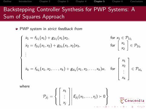
PWP system in strict feedback from
x1 = f1i1(x1) + g1i1(x1)x2, for x1 ∈ P1i1
x2 = f2i2(x1, x2) + g2i2(x1, x2)x3, for
[
x1
x2
]
∈ P2i2
...
xk = fkik (x1, x2, . . . , xk) + gkik (x1, x2, . . . , xk)u, for
x1
x2...xk
∈ Pkik
where
Pjij =
x1...xj
∣
∣
∣
∣
∣
∣
∣
Ejij (x1, . . . , xj) ≻ 0
Outline Introduction Chapter 2 Chapter 3 Chapter 4 Chapter 5 Chapter 6 Conclusions
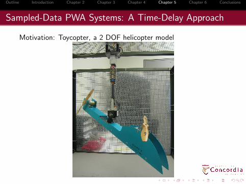
Sampled-Data PWA Systems: A Time-Delay Approach
Motivation: Toycopter, a 2 DOF helicopter model
Outline Introduction Chapter 2 Chapter 3 Chapter 4 Chapter 5 Chapter 6 Conclusions
Sampled-Data PWA Systems: A Time-Delay Approach
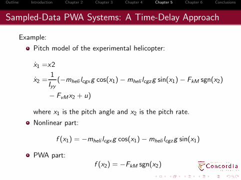
Example:
Pitch model of the experimental helicopter:
x1 =x2
x2 =1
Iyy(−mheli lcgxg cos(x1) − mheli lcgzg sin(x1) − FkM sgn(x2)
− FvMx2 + u)
where x1 is the pitch angle and x2 is the pitch rate.
Nonlinear part:
f (x1) = −mheli lcgxg cos(x1) − mheli lcgzg sin(x1)
PWA part:f (x2) = −FkM sgn(x2)
Outline Introduction Chapter 2 Chapter 3 Chapter 4 Chapter 5 Chapter 6 Conclusions
Sampled-Data PWA Systems: A Time-Delay Approach
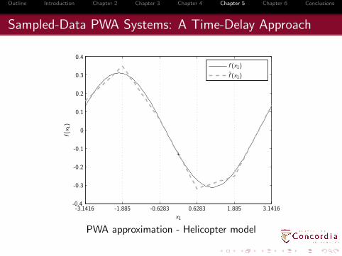
x1
f(x
1)
f (x1)
f (x1)
-3.1416 -1.885 -0.6283 0.6283 1.885 3.1416-0.4
-0.3
-0.2
-0.1
0
0.1
0.2
0.3
0.4
PWA approximation - Helicopter model
Outline Introduction Chapter 2 Chapter 3 Chapter 4 Chapter 5 Chapter 6 Conclusions
Sampled-Data PWA Systems: A Time-Delay Approach
x1
x2
-3 -2 -1 0 1 2 3-2
-1.5
-1
-0.5
0
0.5
1
1.5
2
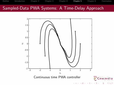
Continuous time PWA controller
Outline Introduction Chapter 2 Chapter 3 Chapter 4 Chapter 5 Chapter 6 Conclusions
Sampled-Data PWA Systems: A Time-Delay Approach
Outline Introduction Chapter 2 Chapter 3 Chapter 4 Chapter 5 Chapter 6 Conclusions
Sampled-Data PWA Systems: A Time-Delay Approach
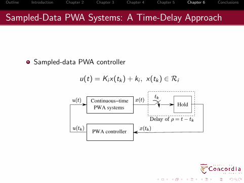
Sampled-data PWA controller
u(t) = Kix(tk) + ki , x(tk) ∈ Ri
Continuous−time
PWA systems
PWA controller
Hold
Outline Introduction Chapter 2 Chapter 3 Chapter 4 Chapter 5 Chapter 6 Conclusions
Sampled-Data PWA Systems: A Time-Delay Approach
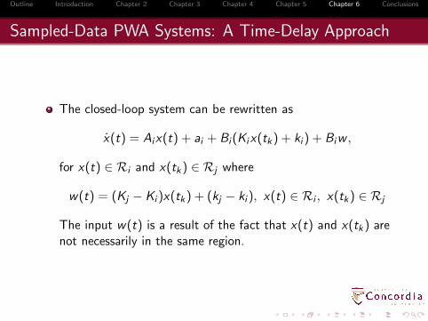
The closed-loop system can be rewritten as
x(t) = Aix(t) + ai + Bi(Kix(tk) + ki ) + Biw ,
for x(t) ∈ Ri and x(tk) ∈ Rj where
w(t) = (Kj − Ki )x(tk) + (kj − ki ), x(t) ∈ Ri , x(tk) ∈ Rj
The input w(t) is a result of the fact that x(t) and x(tk) arenot necessarily in the same region.
Outline Introduction Chapter 2 Chapter 3 Chapter 4 Chapter 5 Chapter 6 Conclusions
Sampled-Data PWA Systems: A Time-Delay Approach
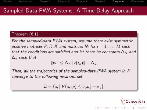
Theorem (6.1)
For the sampled-data PWA system, assume there exist symmetric
positive matrices P ,R ,X and matrices Ni for i = 1, . . . ,M such
that the conditions are satisfied and let there be constants ∆K and
∆k such that
‖w‖ ≤ ∆K‖x(tk)‖ + ∆k
Then, all the trajectories of the sampled-data PWA system in Xconverge to the following invariant set
Ω = xs | V (xs , ρ) ≤ σaµ2θ + σb
Outline Introduction Chapter 2 Chapter 3 Chapter 4 Chapter 5 Chapter 6 Conclusions
Sampled-Data PWA Systems: A Time-Delay Approach
Solving an optimization problem to maximize τM subject to theconstraints of the main theorem and η > γ > 1 leads to
τ⋆M = 0.2193
Outline Introduction Chapter 2 Chapter 3 Chapter 4 Chapter 5 Chapter 6 Conclusions
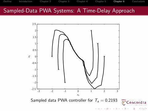
Sampled-Data PWA Systems: A Time-Delay Approach
x1
x2
-3 -2 -1 0 1 2 3-2.5
-2
-1.5
-1
-0.5
0
0.5
1
1.5
2
2.5
Sampled data PWA controller for Ts = 0.2193

Outline Introduction Chapter 2 Chapter 3 Chapter 4 Chapter 5 Chapter 6 Conclusions
Sampled-Data PWA Systems: A Time-Delay Approach
x1
x2
-3 -2 -1 0 1 2 3-2
-1.5
-1
-0.5
0
0.5
1
1.5
2
Continuous time PWA controller
Outline Introduction Chapter 2 Chapter 3 Chapter 4 Chapter 5 Chapter 6 Conclusions
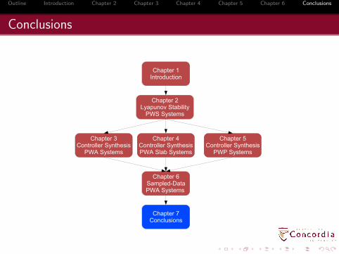
Conclusions
Outline Introduction Chapter 2 Chapter 3 Chapter 4 Chapter 5 Chapter 6 Conclusions
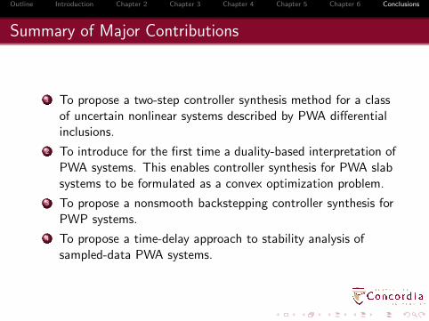
Summary of Major Contributions
1 To propose a two-step controller synthesis method for a classof uncertain nonlinear systems described by PWA differentialinclusions.
2 To introduce for the first time a duality-based interpretation ofPWA systems. This enables controller synthesis for PWA slabsystems to be formulated as a convex optimization problem.
3 To propose a nonsmooth backstepping controller synthesis forPWP systems.
4 To propose a time-delay approach to stability analysis ofsampled-data PWA systems.
Outline Introduction Chapter 2 Chapter 3 Chapter 4 Chapter 5 Chapter 6 Conclusions
Publications
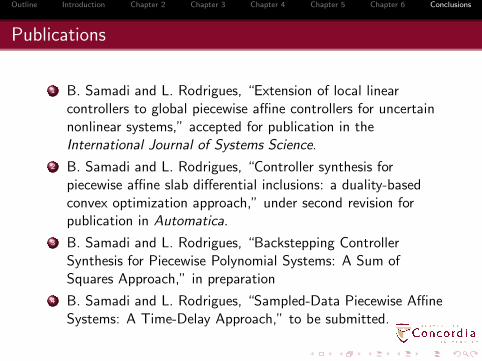
1 B. Samadi and L. Rodrigues, “Extension of local linearcontrollers to global piecewise affine controllers for uncertainnonlinear systems,” accepted for publication in theInternational Journal of Systems Science.
2 B. Samadi and L. Rodrigues, “Controller synthesis forpiecewise affine slab differential inclusions: a duality-basedconvex optimization approach,” under second revision forpublication in Automatica.
3 B. Samadi and L. Rodrigues, “Backstepping ControllerSynthesis for Piecewise Polynomial Systems: A Sum ofSquares Approach,” in preparation
4 B. Samadi and L. Rodrigues, “Sampled-Data Piecewise AffineSystems: A Time-Delay Approach,” to be submitted.
Outline Introduction Chapter 2 Chapter 3 Chapter 4 Chapter 5 Chapter 6 Conclusions
Publications
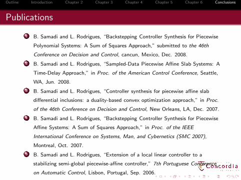
1 B. Samadi and L. Rodrigues, “Backstepping Controller Synthesis for Piecewise
Polynomial Systems: A Sum of Squares Approach,” submitted to the 46th
Conference on Decision and Control, cancun, Mexico, Dec. 2008.
2 B. Samadi and L. Rodrigues, “Sampled-Data Piecewise Affine Slab Systems: A
Time-Delay Approach,” in Proc. of the American Control Conference, Seattle,
WA, Jun. 2008.
3 B. Samadi and L. Rodrigues, “Controller synthesis for piecewise affine slab
differential inclusions: a duality-based convex optimization approach,” in Proc.
of the 46th Conference on Decision and Control, New Orleans, LA, Dec. 2007.
4 B. Samadi and L. Rodrigues, “Backstepping Controller Synthesis for Piecewise
Affine Systems: A Sum of Squares Approach,” in Proc. of the IEEE
International Conference on Systems, Man, and Cybernetics (SMC 2007),
Montreal, Oct. 2007.
5 B. Samadi and L. Rodrigues, “Extension of a local linear controller to a
stabilizing semi-global piecewise-affine controller,” 7th Portuguese Conference
on Automatic Control, Lisbon, Portugal, Sep. 2006.

Outline Introduction Chapter 2 Chapter 3 Chapter 4 Chapter 5 Chapter 6 Conclusions
Questions
Outline Introduction Chapter 2 Chapter 3 Chapter 4 Chapter 5 Chapter 6 Conclusions
Open Problems
Can general PWP/PWA controller synthesis be converted to aconvex problem?
What is the dual of a PWA system?
Outline Introduction Chapter 2 Chapter 3 Chapter 4 Chapter 5 Chapter 6 Conclusions
Special Structure
Type f (x) g(x)
Piecewise Smooth Piecewise Continuous Piecewise Continuous
Piecewise Polynomial Piecewise Polynomial Piecewise Polynomial
Piecewise Affine Piecewise Affine Piecewise Constant
Piecewise Linear Piecewise Linear Piecewise Constant
Linear Linear Constant
Outline Introduction Chapter 2 Chapter 3 Chapter 4 Chapter 5 Chapter 6 Conclusions
Convex Optimization
“In fact the great watershed in optimization is not betweenlinearity and nonlinearity, but convexity andnonconvexity.” (Rockafellar, SIAM review, 1993)
The hard part is to find out if a problem can be formulated asa convex optimization problem.
Outline Introduction Chapter 2 Chapter 3 Chapter 4 Chapter 5 Chapter 6 Conclusions
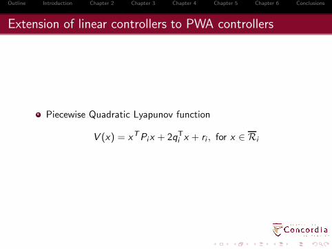
Extension of linear controllers to PWA controllers
Piecewise Quadratic Lyapunov function
V (x) = xTPix + 2qTi x + ri , for x ∈ Ri
Outline Introduction Chapter 2 Chapter 3 Chapter 4 Chapter 5 Chapter 6 Conclusions
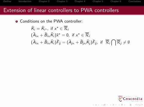
Extension of linear controllers to PWA controllers
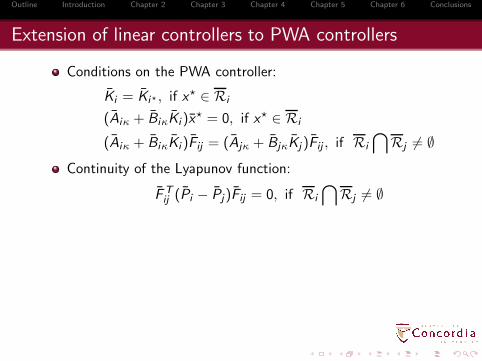
Conditions on the PWA controller:
Ki = Ki⋆ , if x⋆ ∈ Ri
(Aiκ + BiκKi )x⋆ = 0, if x⋆ ∈ Ri
(Aiκ + BiκKi )Fij = (Ajκ + BjκKj )Fij , if Ri
⋂
Rj 6= ∅
Outline Introduction Chapter 2 Chapter 3 Chapter 4 Chapter 5 Chapter 6 Conclusions
Extension of linear controllers to PWA controllers
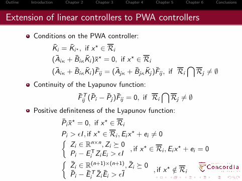
Conditions on the PWA controller:
Ki = Ki⋆ , if x⋆ ∈ Ri
(Aiκ + BiκKi )x⋆ = 0, if x⋆ ∈ Ri
(Aiκ + BiκKi )Fij = (Ajκ + BjκKj )Fij , if Ri
⋂
Rj 6= ∅
Continuity of the Lyapunov function:
FTij (Pi − Pj)Fij = 0, if Ri
⋂
Rj 6= ∅
Outline Introduction Chapter 2 Chapter 3 Chapter 4 Chapter 5 Chapter 6 Conclusions
Extension of linear controllers to PWA controllers
Conditions on the PWA controller:
Ki = Ki⋆ , if x⋆ ∈ Ri
(Aiκ + BiκKi )x⋆ = 0, if x⋆ ∈ Ri
(Aiκ + BiκKi )Fij = (Ajκ + BjκKj )Fij , if Ri
⋂
Rj 6= ∅
Continuity of the Lyapunov function:
FTij (Pi − Pj)Fij = 0, if Ri
⋂
Rj 6= ∅
Positive definiteness of the Lyapunov function:
Pi x⋆ = 0, if x⋆ ∈ Ri
Pi > ǫI , if x⋆ ∈ Ri ,Eix⋆ + ei 6= 0
Zi ∈ Rn×n,Zi 0
Pi − ETi ZiEi > ǫI
, if x⋆ ∈ Ri ,Eix⋆ + ei = 0
Zi ∈ R(n+1)×(n+1), Zi 0
Pi − ETi Zi Ei > ǫI
, if x⋆ /∈ Ri

Outline Introduction Chapter 2 Chapter 3 Chapter 4 Chapter 5 Chapter 6 Conclusions
Extension of linear controllers to PWA controllers
Monotonicity of the Lyapunov function:
for i such that x⋆ ∈ Ri ,Eix⋆ + ei 6= 0,
Pi (Aiκ + BiκKi) + (Aiκ + BiκKi )TPi < −αPi
for i such that x⋆ ∈ Ri ,Eix⋆ + ei = 0,
Λiκ ∈ Rn×n, Λiκ 0
Pi(Aiκ + BiκKi) + (Aiκ + BiκKi)TPi + ET
i ΛiκEi < −αPi
for i such that x⋆ /∈ Ri ,
Λiκ ∈ R(n+1)×(n+1), Λiκ 0
Pi(Aiκ + BiκKi) + (Aiκ + BiκKi)T Pi + ET
i ΛiκEi < −αPi
Outline Introduction Chapter 2 Chapter 3 Chapter 4 Chapter 5 Chapter 6 Conclusions
Extension of linear controllers to PWA controllers
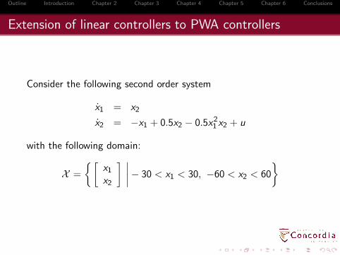
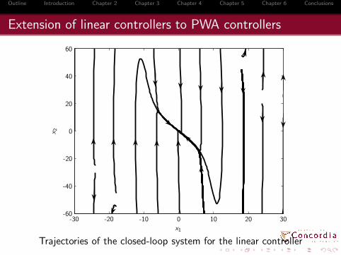
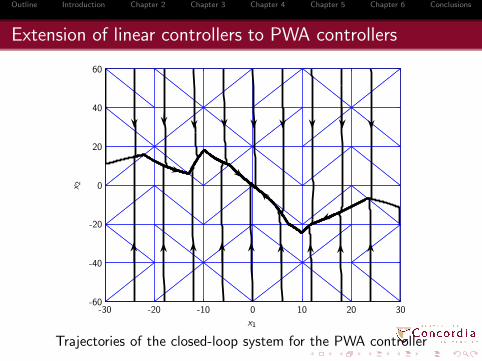
Consider the following second order system
x1 = x2
x2 = −x1 + 0.5x2 − 0.5x21 x2 + u
with the following domain:
X =
[
x1
x2
] ∣
∣
∣
∣
− 30 < x1 < 30, −60 < x2 < 60
Outline Introduction Chapter 2 Chapter 3 Chapter 4 Chapter 5 Chapter 6 Conclusions
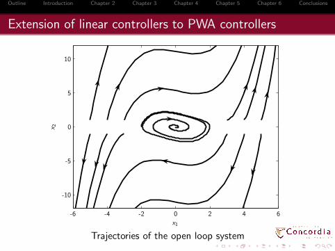
Extension of linear controllers to PWA controllers
x1
x2
-6 -4 -2 0 2 4 6
-10
-5
0
5
10
Trajectories of the open loop system
Outline Introduction Chapter 2 Chapter 3 Chapter 4 Chapter 5 Chapter 6 Conclusions
Extension of linear controllers to PWA controllers
x1
x2
-30 -20 -10 0 10 20 30-60
-40
-20
0
20
40
60
Trajectories of the closed-loop system for the linear controller
Outline Introduction Chapter 2 Chapter 3 Chapter 4 Chapter 5 Chapter 6 Conclusions
Extension of linear controllers to PWA controllers
x1
x2
-30 -20 -10 0 10 20 30-60
-40
-20
0
20
40
60
Trajectories of the closed-loop system for the PWA controller
Outline Introduction Chapter 2 Chapter 3 Chapter 4 Chapter 5 Chapter 6 Conclusions
Extension of linear controllers to PWA controllers
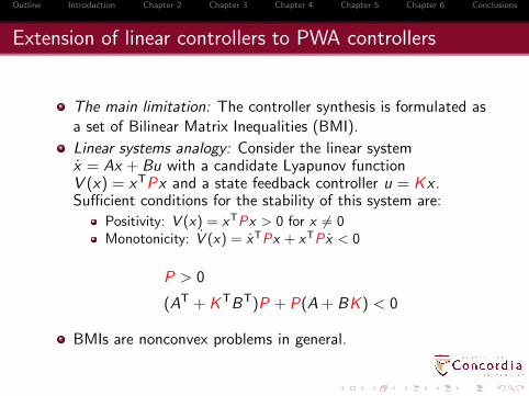
The main limitation: The controller synthesis is formulated asa set of Bilinear Matrix Inequalities (BMI).
Linear systems analogy: Consider the linear systemx = Ax + Bu with a candidate Lyapunov functionV (x) = xTPx and a state feedback controller u = Kx .Sufficient conditions for the stability of this system are:
Positivity: V (x) = xTPx > 0 for x 6= 0Monotonicity: V (x) = xTPx + xTPx < 0
P > 0
(AT + KTBT)P + P(A + BK) < 0
BMIs are nonconvex problems in general.
Outline Introduction Chapter 2 Chapter 3 Chapter 4 Chapter 5 Chapter 6 Conclusions
Extension of linear controllers to PWA controllers
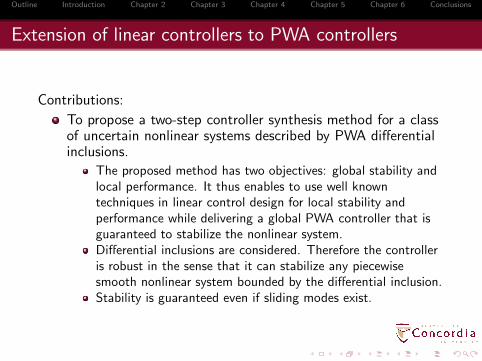
Contributions:
To propose a two-step controller synthesis method for a classof uncertain nonlinear systems described by PWA differentialinclusions.
The proposed method has two objectives: global stability andlocal performance. It thus enables to use well knowntechniques in linear control design for local stability andperformance while delivering a global PWA controller that isguaranteed to stabilize the nonlinear system.Differential inclusions are considered. Therefore the controlleris robust in the sense that it can stabilize any piecewisesmooth nonlinear system bounded by the differential inclusion.Stability is guaranteed even if sliding modes exist.
Outline Introduction Chapter 2 Chapter 3 Chapter 4 Chapter 5 Chapter 6 Conclusions
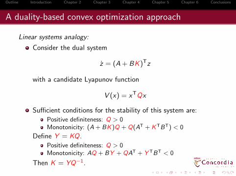
A duality-based convex optimization approach
Linear systems analogy:
Consider the dual system
z = (A + BK)Tz
with a candidate Lyapunov function
V (x) = xTQx
Sufficient conditions for the stability of this system are:
Positive definiteness: Q > 0Monotonicity: (A + BK )Q + Q(AT + KTBT) < 0
Define Y = KQ.
Positive definiteness: Q > 0Monotonicity: AQ + BY + QAT + Y TBT < 0
Then K = YQ−1.

Outline Introduction Chapter 2 Chapter 3 Chapter 4 Chapter 5 Chapter 6 Conclusions
A duality-based convex optimization approach
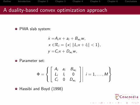
PWA slab system:
x =Aix + ai , x ∈ Ri
Ri =x | ‖Lix + li‖ < 1
Literature
Hassibi and Boyd (1998)Rodrigues and Boyd (2005)
Outline Introduction Chapter 2 Chapter 3 Chapter 4 Chapter 5 Chapter 6 Conclusions
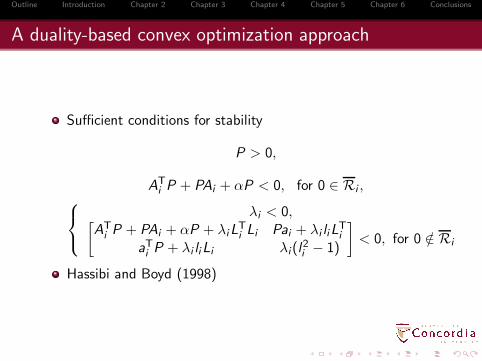
A duality-based convex optimization approach
Sufficient conditions for stability
P > 0,
ATi P + PAi + αP < 0, for 0 ∈ Ri ,
λi < 0,[
ATi P + PAi + αP + λiL
Ti Li Pai + λi liL
Ti
aTi P + λi liLi λi(l
2i − 1)
]
< 0, for 0 /∈ Ri
Hassibi and Boyd (1998)
Outline Introduction Chapter 2 Chapter 3 Chapter 4 Chapter 5 Chapter 6 Conclusions
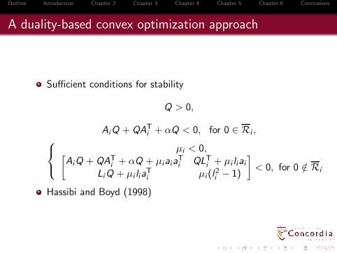
A duality-based convex optimization approach
Sufficient conditions for stability
Q > 0,
AiQ + QATi + αQ < 0, for 0 ∈ Ri ,
µi < 0,[
AiQ + QATi + αQ + µiaia
Ti QLT
i + µi liai
LiQ + µi liaTi µi(l
2i − 1)
]
< 0, for 0 /∈ Ri
Hassibi and Boyd (1998)
Outline Introduction Chapter 2 Chapter 3 Chapter 4 Chapter 5 Chapter 6 Conclusions
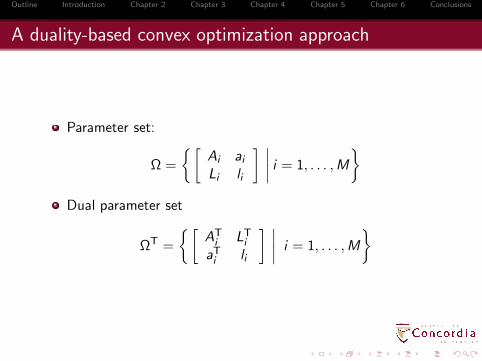
A duality-based convex optimization approach
Parameter set:
Ω =
[
Ai ai
Li li
] ∣
∣
∣
∣
i = 1, . . . ,M
Dual parameter set
ΩT =
[
ATi LT
i
aTi li
] ∣
∣
∣
∣
i = 1, . . . ,M
Outline Introduction Chapter 2 Chapter 3 Chapter 4 Chapter 5 Chapter 6 Conclusions
A duality-based convex optimization approach
PWA slab system:
x =Aix + ai + Bwiw ,
x ∈Ri = x | ‖Lix + li‖ < 1,
y =Cix + Dwiw ,
Parameter set:
Φ =
Ai ai Bwi
Li li 0Ci 0 Dwi
∣
∣
∣
∣
∣
∣
i = 1, . . . ,M
Hassibi and Boyd (1998)
Outline Introduction Chapter 2 Chapter 3 Chapter 4 Chapter 5 Chapter 6 Conclusions
A duality-based convex optimization approach
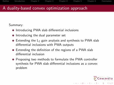
Summary:
Introducing PWA slab differential inclusions
Introducing the dual parameter set
Extending the L2 gain analysis and synthesis to PWA slabdifferential inclusions with PWA outputs
Extending the definition of the regions of a PWA slabdifferential inclusion
Proposing two methods to formulate the PWA controllersynthesis for PWA slab differential inclusions as a convexproblem
Outline Introduction Chapter 2 Chapter 3 Chapter 4 Chapter 5 Chapter 6 Conclusions
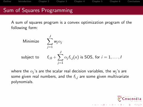
Sum of Squares Programming
A sum of squares program is a convex optimization program of thefollowing form:
Minimize
J∑
j=1
wjαj
subject to fi ,0 +J∑
j=1
αj fi ,j(x) is SOS, for i = 1, . . . , I
where the αj ’s are the scalar real decision variables, the wj ’s aresome given real numbers, and the fi ,j are some given multivariatepolynomials.
Outline Introduction Chapter 2 Chapter 3 Chapter 4 Chapter 5 Chapter 6 Conclusions
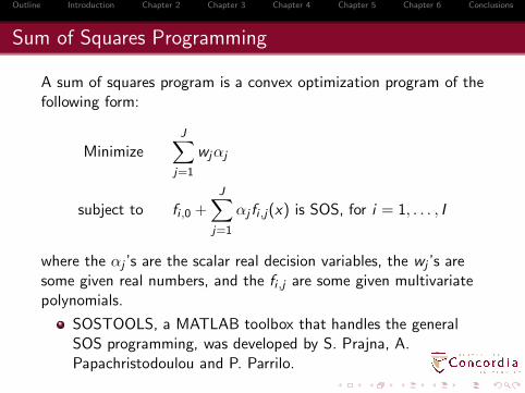
Sum of Squares Programming
A sum of squares program is a convex optimization program of thefollowing form:
Minimize
J∑
j=1
wjαj
subject to fi ,0 +J∑
j=1
αj fi ,j(x) is SOS, for i = 1, . . . , I
where the αj ’s are the scalar real decision variables, the wj ’s aresome given real numbers, and the fi ,j are some given multivariatepolynomials.
SOSTOOLS, a MATLAB toolbox that handles the generalSOS programming, was developed by S. Prajna, A.Papachristodoulou and P. Parrilo.
Outline Introduction Chapter 2 Chapter 3 Chapter 4 Chapter 5 Chapter 6 Conclusions
Backstepping Controller Synthesis for PWP Systems: A
Sum of Squares Approach
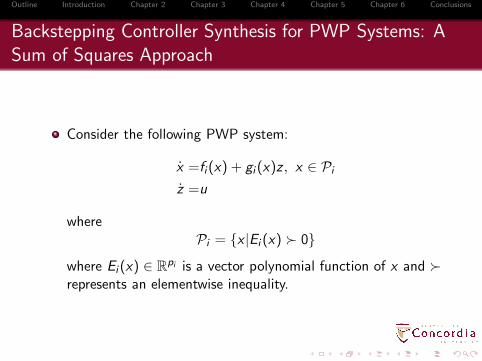
Consider the following PWP system:
x =fi(x) + gi (x)z , x ∈ Pi
z =u
wherePi = x |Ei (x) ≻ 0
where Ei (x) ∈ Rpi is a vector polynomial function of x and ≻
represents an elementwise inequality.
Outline Introduction Chapter 2 Chapter 3 Chapter 4 Chapter 5 Chapter 6 Conclusions
Backstepping Controller Synthesis for PWP Systems: A
Sum of Squares Approach
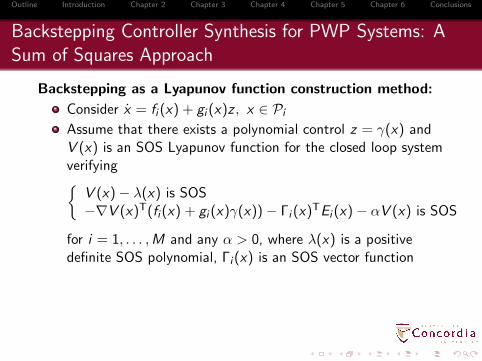
Backstepping as a Lyapunov function construction method:
Consider x = fi (x) + gi (x)z , x ∈ Pi
Outline Introduction Chapter 2 Chapter 3 Chapter 4 Chapter 5 Chapter 6 Conclusions
Backstepping Controller Synthesis for PWP Systems: A
Sum of Squares Approach
Backstepping as a Lyapunov function construction method:
Consider x = fi (x) + gi (x)z , x ∈ Pi
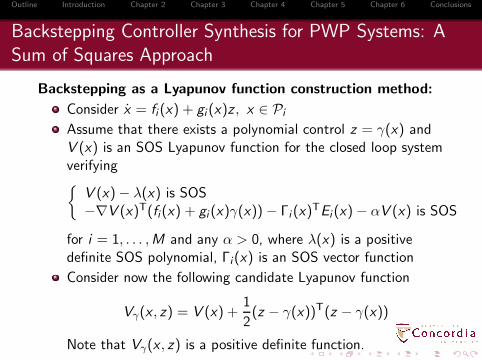
Assume that there exists a polynomial control z = γ(x) andV (x) is an SOS Lyapunov function for the closed loop systemverifying
V (x) − λ(x) is SOS−∇V (x)T(fi(x) + gi (x)γ(x)) − Γi (x)TEi (x) − αV (x) is SOS
for i = 1, . . . ,M and any α > 0, where λ(x) is a positivedefinite SOS polynomial, Γi(x) is an SOS vector function
Outline Introduction Chapter 2 Chapter 3 Chapter 4 Chapter 5 Chapter 6 Conclusions
Backstepping Controller Synthesis for PWP Systems: A
Sum of Squares Approach
Backstepping as a Lyapunov function construction method:
Consider x = fi (x) + gi (x)z , x ∈ Pi
Assume that there exists a polynomial control z = γ(x) andV (x) is an SOS Lyapunov function for the closed loop systemverifying
V (x) − λ(x) is SOS−∇V (x)T(fi(x) + gi (x)γ(x)) − Γi (x)TEi (x) − αV (x) is SOS
for i = 1, . . . ,M and any α > 0, where λ(x) is a positivedefinite SOS polynomial, Γi(x) is an SOS vector function
Consider now the following candidate Lyapunov function
Vγ(x , z) = V (x) +1
2(z − γ(x))T(z − γ(x))
Note that Vγ(x , z) is a positive definite function.
Outline Introduction Chapter 2 Chapter 3 Chapter 4 Chapter 5 Chapter 6 Conclusions
Backstepping Controller Synthesis for PWP Systems: A
Sum of Squares Approach
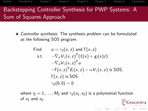
Controller synthesis: The synthesis problem can be formulatedas the following SOS program.
Find u = γ2(x , z) and Γ(x , z)
s.t. −∇xVγ(x , z)T(fi(x) + gi (x)z)
−∇zVγ(x , z)Tu
−Γ(x , z)TEi (x , z) − αVγ(x , z) is SOS,
Γ(x , z) is SOS
γ2(0, 0) = 0
where i2 = 1, . . . ,M2 and γ2(x1, x2) is a polynomial functionof x1 and x2.
Outline Introduction Chapter 2 Chapter 3 Chapter 4 Chapter 5 Chapter 6 Conclusions
Backstepping Controller Synthesis for PWP Systems: A
Sum of Squares Approach
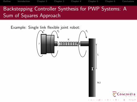
Example: Single link flexible joint robot:
Outline Introduction Chapter 2 Chapter 3 Chapter 4 Chapter 5 Chapter 6 Conclusions
Backstepping Controller Synthesis for PWP Systems: A
Sum of Squares Approach
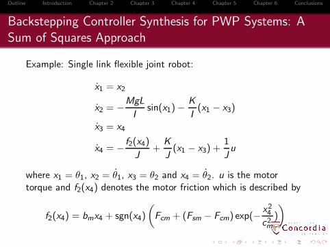
Example: Single link flexible joint robot:
x1 = x2
x2 = −MgL
Isin(x1) −
K
I(x1 − x3)
x3 = x4
x4 = −f2(x4)
J+
K
J(x1 − x3) +
1
Ju
where x1 = θ1, x2 = θ1, x3 = θ2 and x4 = θ2. u is the motortorque and f2(x4) denotes the motor friction which is described by
f2(x4) = bmx4 + sgn(x4)
(
Fcm + (Fsm − Fcm) exp(−x24
c2m
)
)
Outline Introduction Chapter 2 Chapter 3 Chapter 4 Chapter 5 Chapter 6 Conclusions
Backstepping Controller Synthesis for PWP Systems: A
Sum of Squares Approach
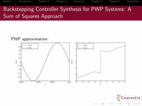
PWP approximation:
x1
f 1(x
1)
f1(x1)
f1(x1)
-3.1416 -0.8976 0.8976 3.1416-1
-0.8
-0.6
-0.4
-0.2
0
0.2
0.4
0.6
0.8
1
x4
f 2(x
4)
f2(x4)
f2(x4)
-8 -6 -4 -2 0 2 4 6 8-3
-2
-1
0
1
2
3
Outline Introduction Chapter 2 Chapter 3 Chapter 4 Chapter 5 Chapter 6 Conclusions
Backstepping Controller Synthesis for PWP Systems: A
Sum of Squares Approach
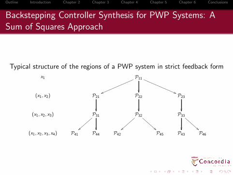
Typical structure of the regions of a PWP system in strict feedback form
x1 P11
vvmmmmmmmmmmmmmmmm
((QQQQQQQQQQQQQQQQ
(x1, x2) P21
P22
P23
(x1, x2, x3) P31
P32
!!CC
CCCC
CCP33
!!CC
CCCC
CC
(x1, x2, x3, x4) P41 P44 P42 P45 P43 P46
Outline Introduction Chapter 2 Chapter 3 Chapter 4 Chapter 5 Chapter 6 Conclusions
Backstepping Controller Synthesis for PWP Systems: A
Sum of Squares Approach
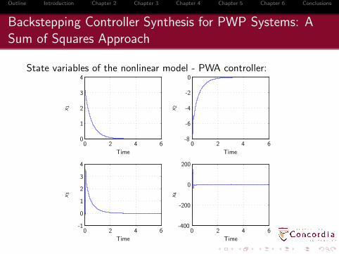
State variables of the nonlinear model - PWA controller:
Time
x1
Time
x2
Time
x3
Time
x4
0 2 4 60 2 4 6
0 2 4 60 2 4 6
-400
-200
0
200
-1
0
1
2
3
4
-8
-6
-4
-2
0
0
1
2
3
4
Outline Introduction Chapter 2 Chapter 3 Chapter 4 Chapter 5 Chapter 6 Conclusions
Backstepping Controller Synthesis for PWP Systems: A
Sum of Squares Approach
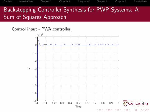
Control input - PWA controller:
Time
u
0 0.1 0.2 0.3 0.4 0.5 0.6 0.7 0.8 0.9 1-7
-6
-5
-4
-3
-2
-1
0
1×10⁴
Outline Introduction Chapter 2 Chapter 3 Chapter 4 Chapter 5 Chapter 6 Conclusions
Backstepping Controller Synthesis for PWP Systems: A
Sum of Squares Approach
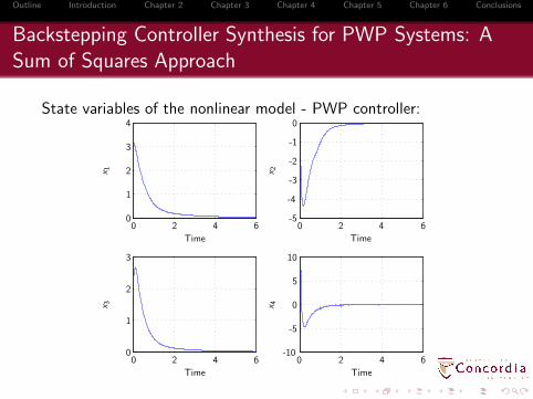
State variables of the nonlinear model - PWP controller:
Time
x1
Time
x2
Time
x3
Time
x4
0 2 4 60 2 4 6
0 2 4 60 2 4 6
-10
-5
0
5
10
0
1
2
3
-5
-4
-3
-2
-1
0
0
1
2
3
4
Outline Introduction Chapter 2 Chapter 3 Chapter 4 Chapter 5 Chapter 6 Conclusions
Backstepping Controller Synthesis for PWP Systems: A
Sum of Squares Approach
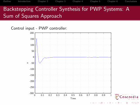
Control input - PWP controller:
Time
u
0 0.1 0.2 0.3 0.4 0.5 0.6 0.7 0.8 0.9 1-300
-250
-200
-150
-100
-50
0
50
100
150
200
Outline Introduction Chapter 2 Chapter 3 Chapter 4 Chapter 5 Chapter 6 Conclusions
Backstepping Controller Synthesis for PWP Systems: A
Sum of Squares Approach
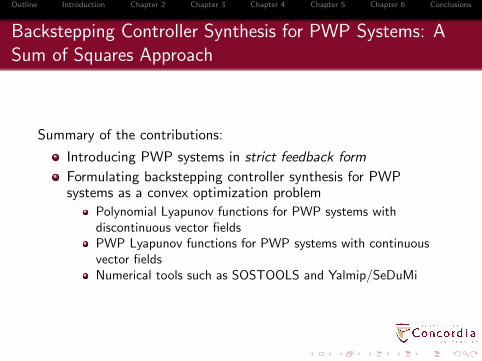
Summary of the contributions:
Introducing PWP systems in strict feedback form
Formulating backstepping controller synthesis for PWPsystems as a convex optimization problem
Polynomial Lyapunov functions for PWP systems withdiscontinuous vector fieldsPWP Lyapunov functions for PWP systems with continuousvector fieldsNumerical tools such as SOSTOOLS and Yalmip/SeDuMi
Outline Introduction Chapter 2 Chapter 3 Chapter 4 Chapter 5 Chapter 6 Conclusions
Sampled-Data PWA Systems: A Time-Delay Approach
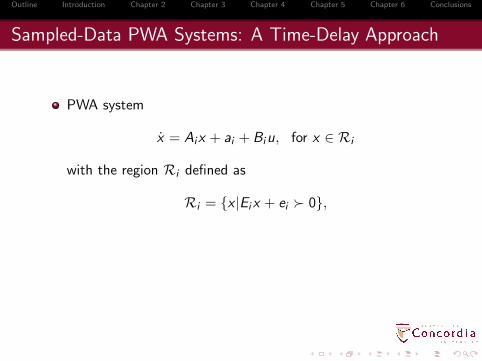
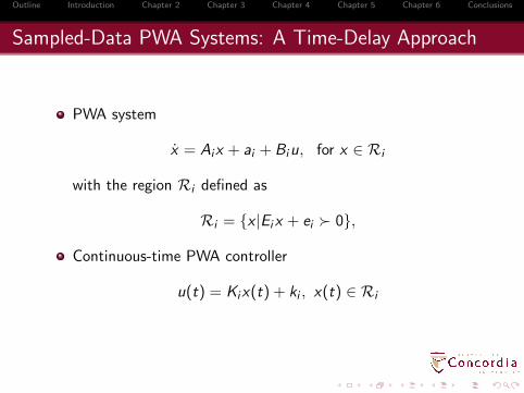
PWA system
x = Aix + ai + Biu, for x ∈ Ri
with the region Ri defined as
Ri = x |Eix + ei ≻ 0,
Outline Introduction Chapter 2 Chapter 3 Chapter 4 Chapter 5 Chapter 6 Conclusions
Sampled-Data PWA Systems: A Time-Delay Approach
PWA system
x = Aix + ai + Biu, for x ∈ Ri
with the region Ri defined as
Ri = x |Eix + ei ≻ 0,
Continuous-time PWA controller
u(t) = Kix(t) + ki , x(t) ∈ Ri
Outline Introduction Chapter 2 Chapter 3 Chapter 4 Chapter 5 Chapter 6 Conclusions
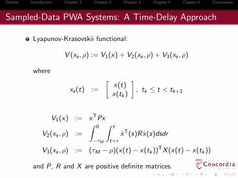
Sampled-Data PWA Systems: A Time-Delay Approach
Lyapunov-Krasovskii functional:
V (xs , ρ) := V1(x) + V2(xs , ρ) + V3(xs , ρ)
where
xs(t) :=
[
x(t)x(tk)
]
, tk ≤ t < tk+1
V1(x) := xTPx
V2(xs , ρ) :=
∫ 0
−τM
∫ t
t+rxT(s)Rx(s)dsdr
V3(xs , ρ) := (τM − ρ)(x(t) − x(tk))TX (x(t) − x(tk))
and P , R and X are positive definite matrices.
Outline Introduction Chapter 2 Chapter 3 Chapter 4 Chapter 5 Chapter 6 Conclusions
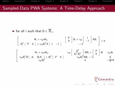
Sampled-Data PWA Systems: A Time-Delay Approach
for all i such that 0 ∈ Ri ,
Ψi + τMM1i
[
P0
]
Bi + τM
[
I−I
]
XBi
BTi
[
P 0]
+ τMBTi X
[
I −I]
−γI
< 0
Ψi + τMM2i τM
[
ATi
KTi BT
i
]
RBi +
[
P0
]
Bi τMNi
τMBTi R
[
Ai BiKi
]
+ BTi
[
P 0]
τMBTi RBi − γI 0
τMNTi 0 −
τM2
R
Outline Introduction Chapter 2 Chapter 3 Chapter 4 Chapter 5 Chapter 6 Conclusions
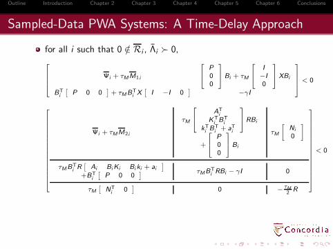
Sampled-Data PWA Systems: A Time-Delay Approach
for all i such that 0 /∈ Ri , Λi ≻ 0,
Ψi + τMM1 i
P00
Bi + τM
I−I0
XBi
BTi
[
P 0 0]
+ τMBTi X
[
I −I 0]
−γI
< 0
Ψi + τMM2i
τM
ATi
KTi BT
ikTi BT
i + aTi
RBi
+
P00
Bi
τM
[
Ni
0
]
τMBTi R
[
Ai BiKi Biki + ai
]
+BTi
[
P 0 0] τMBT
i RBi − γI 0
τM
[
NTi 0
]
0 −τM2
R
< 0
Outline Introduction Chapter 2 Chapter 3 Chapter 4 Chapter 5 Chapter 6 Conclusions
Sampled-Data PWA Systems: A Time-Delay Approach
Summary of the contributions
Formulating stability analysis of sampled-data PWA systemsas a convex optimization problem
Outline Introduction Chapter 2 Chapter 3 Chapter 4 Chapter 5 Chapter 6 Conclusions
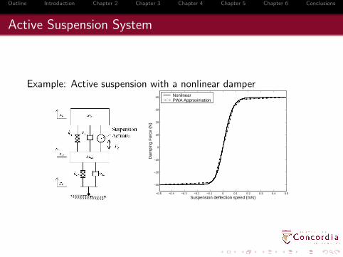
Active Suspension System
Example: Active suspension with a nonlinear damper
−0.5 −0.4 −0.3 −0.2 −0.1 0 0.1 0.2 0.3 0.4 0.5
−30
−20
−10
0
10
20
30
40
Suspension deflection speed (m/s)
Dam
ping
For
ce (
N)
NonlinearPWA Approximation
![Lipschitzian Piecewise Smooth Minimization [0.5ex] via ... EuroAd Workshop - Sabrina Fieg… · Lipschitzian Piecewise Smooth Minimization via Algorithmic Differentiation Sabrina](https://img.pdfslide.net/doc/110x75/5fc48388ca73b406955dcfd3/lipschitzian-piecewise-smooth-minimization-05ex-via-euroad-workshop-sabrina.jpg)

![Fourier reconstruction of univariate piecewise …platte/pub/Driver_ACHArevised.pdf · Fourier reconstruction of univariate piecewise-smooth functions from ... FFT [9 {12], the](https://img.pdfslide.net/doc/110x75/5b982e4609d3f2b16c8b6ab2/fourier-reconstruction-of-univariate-piecewise-plattepubdriver-fourier-reconstruction.jpg)