Computers & Fluids 39 (2010) 1146–1155

Contents lists available at ScienceDirect

Computers & Fluids

journal homepage: www.elsevier .com/locate /compfluid

On the effect of wind direction and urban surroundings on natural ventilationof a large semi-enclosed stadium

T. van Hooff a,b,*,1, B. Blocken a

a Building Physics and Systems, Eindhoven University of Technology, P.O. Box 513, 5600 MB Eindhoven, The Netherlandsb Laboratory of Building Physics, Katholieke Universiteit Leuven, Kasteelpark Arenberg 40, 3001 Leuven, Belgium

a r t i c l e i n f o

Article history:Received 23 November 2009Received in revised form 11 February 2010Accepted 17 February 2010Available online 21 February 2010

Keywords:Natural ventilationWind directionComputational Fluid Dynamics (CFD)Numerical simulationModel validationCross-ventilation

0045-7930/$ - see front matter � 2010 Elsevier Ltd. Adoi:10.1016/j.compfluid.2010.02.004

* Corresponding author. Address: Building PhysiUniversity of Technology, P.O. Box 513, 5600 MB ETel.: +31 (0) 40 247 5877; fax: +31 (0) 40 243 8595.

E-mail address: t.a.j.v.hooff@tue.nl (T. van Hooff).1 Twan van Hooff is a PhD student at both Eindhoven

the Katholieke Universiteit Leuven.

a b s t r a c t

Natural ventilation of buildings refers to the replacement of indoor air with outdoor air due to pressuredifferences caused by wind and/or buoyancy. It is often expressed in terms of the air change rate per hour(ACH). The pressure differences created by the wind depend – among others – on the wind speed, thewind direction, the configuration of surrounding buildings and the surrounding topography. Computa-tional Fluid Dynamics (CFD) has been used extensively in natural ventilation research. However, mostCFD studies were performed for only a limited number of wind directions and/or without consideringthe urban surroundings. This paper presents isothermal CFD simulations of coupled urban wind flowand indoor natural ventilation to assess the influence of wind direction and urban surroundings on theACH of a large semi-enclosed stadium. Simulations are performed for eight wind directions and for acomputational model with and without the surrounding buildings. CFD solution verification is conductedby performing a grid-sensitivity analysis. CFD validation is performed with on-site wind velocity mea-surements. The simulated differences in ACH between wind directions can go up to 75% (without sur-rounding buildings) and 152% (with surrounding buildings). Furthermore, comparing the simulationswith and without surrounding buildings showed that neglecting the surroundings can lead to overesti-mations of the ACH with up to 96%.

� 2010 Elsevier Ltd. All rights reserved.

1. Introduction

Environmental awareness and the decreasing availability of fos-sil fuels have led to an increased interest in more sustainable waysto ensure a healthy and comfortable indoor environment in build-ings. Natural ventilation can be an important approach in this re-spect. It refers to ventilation induced by either wind flow orbuoyancy (stack), or a combination of these two driving forces.Whereas natural ventilation is based on natural driving forces,mechanical ventilation uses energy consuming fans to supply airinto the building. The feasibility of natural ventilation of buildingsdepends on several parameters such as the geometry of the build-ing itself, the geometry of the surrounding buildings, the surround-ing topography and the wind statistics including prevailing winddirection. Although natural ventilation of buildings has been ap-plied since centuries, it is still an intensive area of research due

ll rights reserved.

cs and Systems, Eindhovenindhoven, The Netherlands.

University of Technology and

to both its complexity and its potential for sustainable building de-sign and operation.

A large body of research exists on natural ventilation, based ontheory [1–3], analytical work [4–6], experiments [7–10] andnumerical simulation with Computational Fluid Dynamics (CFD)[6,7,9,11–19]. CFD has some clear advantages compared to otherapproaches. Theoretical and analytical approaches are very valu-able to provide general insights but are less suitable when complexgeometrical configurations are involved. With full-scale (on-site)measurements, many of the influencing parameters (e.g. meteoro-logical conditions) cannot be controlled, and the measurements areusually only performed at a few sampling positions. Furthermore,on-site measurements are not an option in the design stage, whenthe buildings under study have not yet been constructed. Reduced-scale wind tunnel measurements allow controlling the influencingparameters, but the measurements are often only point measure-ments at a few selected positions. In addition, reduced-scale windtunnel testing can be hampered by similarity requirements. This isparticularly the case for large city models or for buildings withsmall ventilation openings (due to Reynolds number effects), aswell as with non-isothermal wind tunnel experiments. The mainadvantages of CFD are that it allows full control over the influenc-ing parameters and that it provides detailed information on all rel-

T. van Hooff, B. Blocken / Computers & Fluids 39 (2010) 1146–1155 1147

evant parameters simultaneously in all points of the computationaldomain (whole flow-field data). Because the simulations can beperformed at full scale, CFD simulations do not suffer from similar-ity requirements. However, CFD accuracy and reliability are mainconcerns, and therefore CFD verification and validation studiesare imperative.

In spite of the large amount of natural ventilation studies per-formed in the past, detailed studies on the effect of both winddirection and surrounding buildings on natural ventilation arelacking. This effect is especially important to assess the feasibilityof natural ventilation in suburban and urban environments. In suchenvironments, surrounding buildings can provide significant shel-ter from wind, but could also increase the wind exposure due tochanneling effects [20–22]. The influence of the surrounding build-ings can be very different depending on the wind direction. Giventhe disadvantages of experimental approaches, CFD seems themost suitable tool for such investigations. Past computational re-search efforts in this area could be divided into two categories:(1) studies for isolated buildings, in which the effect of wind direc-tion is due to building geometry and the position of the ventilationopenings; and (2) studies for non-isolated buildings, in which theeffect of wind direction on natural ventilation is due to the com-bined effect of surrounding buildings, building geometry and theposition of the ventilation openings. Several studies of the first cat-egory exist, which have confirmed the large influence of winddirection. Studies of the second category however are ratherscarce. A brief overview of studies in each category is given below.

Horan and Finn [15] examined the ACH of a free-standing two-storey naturally ventilated building for four wind directions usingCFD and found large variations in ACH between the wind direc-tions, from an ACH value of 3.5 to 15 h�1. More recently, Teitelet al. [16] and Norton et al. [17] performed CFD simulations of nat-ural ventilation in agricultural buildings situated in open terrain.Teitel et al. [16] studied the air flow in one of four clustered green-houses for four wind directions with an interval of 30� and foundsignificant differences in air flow patterns and ACH (up to 56%).Norton et al. [17] studied the ventilation effectiveness in livestockbuildings for wind directions ranging from 0� to 90� with an inter-val of 10� and found differences in ACH up to 100% depending onthe wind direction. Note that all of the aforementioned CFD studiesdid not consider urban surroundings. Differences in ACH weretherefore the result of asymmetry of the building geometry and/or the position of the ventilation openings.

Only a few studies concerning the influence of the building sur-roundings on natural ventilation and natural ventilation potentialare reported in the literature, however most of them are not CFDstudies. One example of a CFD study in which a part of the sur-roundings was included was conducted by Jiang and Chen [18].They performed Large Eddy Simulations (LES) of fluctuating winddirections to assess the natural ventilation of an apartment in afive-storey high building. The computational domain included ninesurrounding buildings in the vicinity of the studied building; otherparts of the urban surroundings were not included. This studyshowed the important influence of short term fluctuations of winddirection within a range of 80� during a short time period of15 min. As opposed to the present study however, it did not con-sider different steady wind directions. Wirén [23] studied theinfluence of surrounding buildings on wind pressure distributionsand ventilative heat losses in a wind tunnel and found that intro-ducing surrounding buildings changed the measured pressure dis-tributions considerably. The influence of surrounding buildings hasalso been studied by van Moeseke et al. [24]. However, this studywas performed using a software package for the thermal analysisof buildings that includes a 2D CFD module. The package calculatedthe ACH of the building using pressure coefficients obtained from aparametrical model. It indicated the strong influence of both wind

direction and building surroundings. Van Moeseke et al. [24]stressed the unsuitability of parametrical models to accurately as-sess the wind flow in urban environments, but stated that themethod used in their paper might be useful for architects to obtainsome first view on the feasibility of natural ventilation. The reviewpaper by Costola et al. [25] on pressure coefficient databases fornatural ventilation studies also indicates that very few data existon the effect of urban surroundings and the related sheltering ef-fects. To the knowledge of the authors, detailed CFD studies onthe effect of wind direction and surrounding buildings on indoornatural ventilation in urban environments have not yet beenperformed.

This paper presents a study on the effect of wind direction andurban surroundings on the natural ventilation of the semi-enclosedAmsterdam ArenA stadium in the Netherlands. It is situated in anurban environment with medium to high-rise buildings. Since noHVAC systems are incorporated, natural ventilation is the onlymeans to maintain a healthy and comfortable indoor environment.In a previous study for this stadium, van Hooff and Blocken [19]indicated that the ACH can be insufficient when spectators arepresent and the stadium roof is closed during summer. Since thisprevious study focused on the fully coupled outdoor–indoor simu-lation approach and on the proposed body-fitted grid generationtechnique, only a few wind directions were studied at that time.In the present paper, the effects of wind direction and urban sur-roundings on natural ventilation are analyzed in detail. Simula-tions are performed for eight wind directions using the fullycoupled simulation approach, in which outdoor wind flow and in-door air flow are computed simultaneously in the same computa-tional domain. Furthermore, simulations are performed with andwithout the surrounding buildings to assess the influence of thesurroundings on the ACH. The turbulent wind flow is obtained bysolving the 3D steady Reynolds-Averaged Navier–Stokes (RANS)equations in combination with the realizable k–e turbulence modelby Shih et al. [26] and the standard wall functions by Launder andSpalding [27] with roughness modifications by Cebeci and Brad-shaw [28]. A grid-sensitivity analysis is performed for CFD solutionverification. The CFD model is validated using full-scale windvelocity measurements.

In Section 2, the geometry of stadium and surroundings isbriefly described. The computational model is outlined in Section 3.Section 4 contains the model validation. The simulation results aregiven in Section 5. Sections 6 (discussion) and 7 (conclusions) con-clude the paper.

2. Description of stadium and surroundings

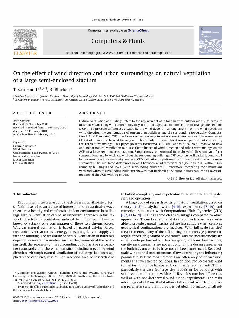
The Amsterdam ArenA is a multifunctional dome-shaped sta-dium with a movable and semi-transparent roof. Fig. 1a showsan aerial view of the stadium with the roof in closed positionand Fig. 1b shows a view from street level. Fig. 2a–c provide a de-tailed plan view and the two cross-sections aa0 and bb0. The exte-rior stadium dimensions are 226 � 190 � 72 m3 (L �W � H). Thestadium has a capacity of 51,628 seated spectators and an interiorvolume of about 1.2 � 106 m3. The roof can be closed by movingtwo large panels with a projected horizontal area of 110 � 40 m2

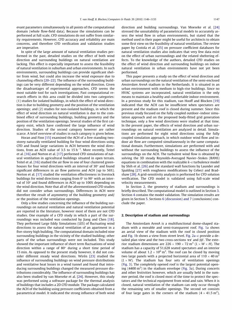
(L �W). The stadium has four sets of ventilation openings(Fig. 3). The completely opened roof is the largest potential open-ing (4400 m2) in the stadium envelope (Fig. 3a). During concertsand other festivities however, which are usually held in the sum-mer period, the roof is closed most of the time to protect the spec-tators and the technical equipment from wind and rain. When it isclosed, natural ventilation of the stadium can only occur throughthe remaining sets of smaller openings. The second set consistsof four large gates in the corners of the stadium (4 � 41.5 m2),

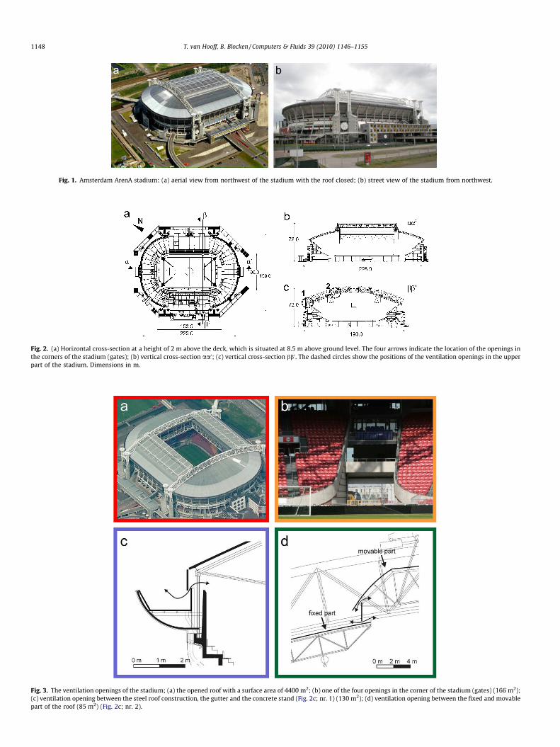
Fig. 1. Amsterdam ArenA stadium: (a) aerial view from northwest of the stadium with the roof closed; (b) street view of the stadium from northwest.

Fig. 2. (a) Horizontal cross-section at a height of 2 m above the deck, which is situated at 8.5 m above ground level. The four arrows indicate the location of the openings inthe corners of the stadium (gates); (b) vertical cross-section aa0; (c) vertical cross-section bb0 . The dashed circles show the positions of the ventilation openings in the upperpart of the stadium. Dimensions in m.

Fig. 3. The ventilation openings of the stadium; (a) the opened roof with a surface area of 4400 m2; (b) one of the four openings in the corner of the stadium (gates) (166 m2);(c) ventilation opening between the steel roof construction, the gutter and the concrete stand (Fig. 2c; nr. 1) (130 m2); (d) ventilation opening between the fixed and movablepart of the roof (85 m2) (Fig. 2c; nr. 2).

1148 T. van Hooff, B. Blocken / Computers & Fluids 39 (2010) 1146–1155

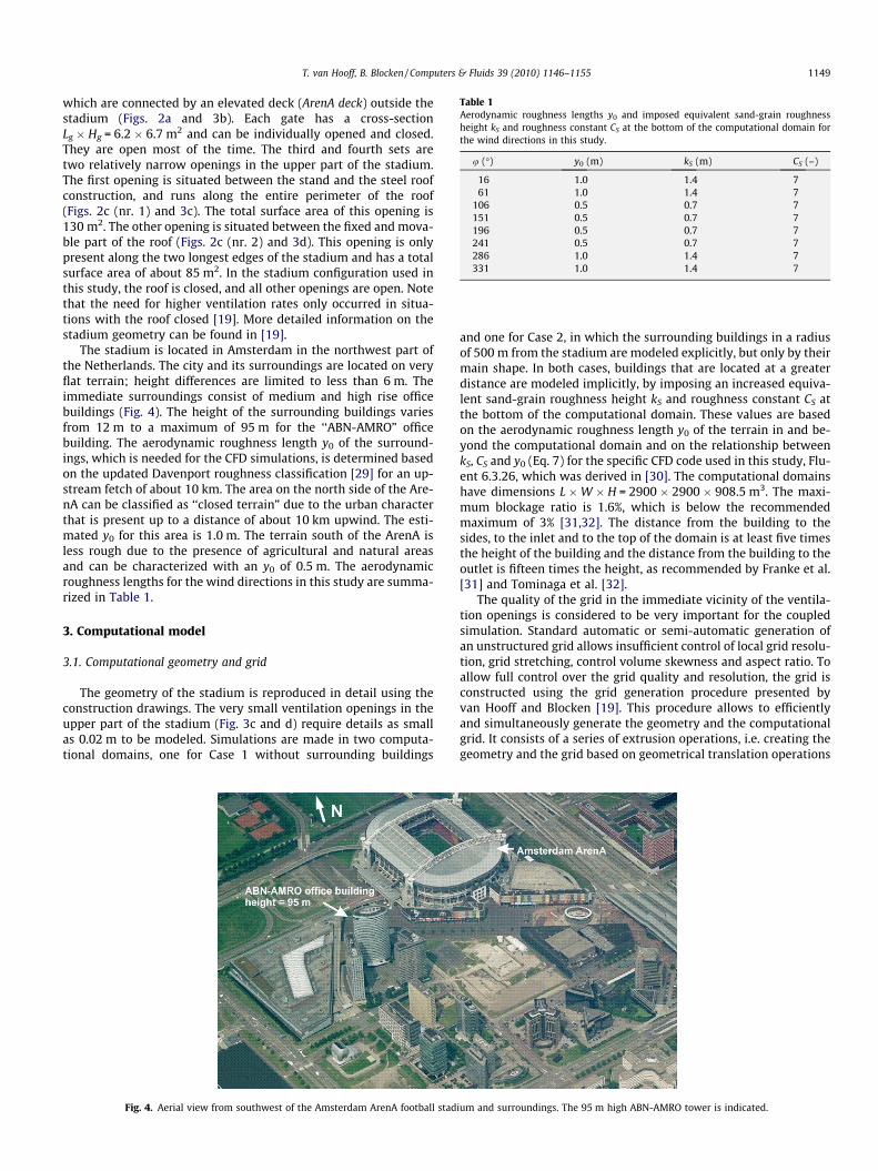
Table 1Aerodynamic roughness lengths y0 and imposed equivalent sand-grain roughnessheight kS and roughness constant CS at the bottom of the computational domain forthe wind directions in this study.

u (�) y0 (m) kS (m) CS (–)

16 1.0 1.4 761 1.0 1.4 7

106 0.5 0.7 7151 0.5 0.7 7196 0.5 0.7 7241 0.5 0.7 7286 1.0 1.4 7331 1.0 1.4 7

T. van Hooff, B. Blocken / Computers & Fluids 39 (2010) 1146–1155 1149

which are connected by an elevated deck (ArenA deck) outside thestadium (Figs. 2a and 3b). Each gate has a cross-sectionLg � Hg = 6.2 � 6.7 m2 and can be individually opened and closed.They are open most of the time. The third and fourth sets aretwo relatively narrow openings in the upper part of the stadium.The first opening is situated between the stand and the steel roofconstruction, and runs along the entire perimeter of the roof(Figs. 2c (nr. 1) and 3c). The total surface area of this opening is130 m2. The other opening is situated between the fixed and mova-ble part of the roof (Figs. 2c (nr. 2) and 3d). This opening is onlypresent along the two longest edges of the stadium and has a totalsurface area of about 85 m2. In the stadium configuration used inthis study, the roof is closed, and all other openings are open. Notethat the need for higher ventilation rates only occurred in situa-tions with the roof closed [19]. More detailed information on thestadium geometry can be found in [19].

The stadium is located in Amsterdam in the northwest part ofthe Netherlands. The city and its surroundings are located on veryflat terrain; height differences are limited to less than 6 m. Theimmediate surroundings consist of medium and high rise officebuildings (Fig. 4). The height of the surrounding buildings variesfrom 12 m to a maximum of 95 m for the ‘‘ABN-AMRO” officebuilding. The aerodynamic roughness length y0 of the surround-ings, which is needed for the CFD simulations, is determined basedon the updated Davenport roughness classification [29] for an up-stream fetch of about 10 km. The area on the north side of the Are-nA can be classified as ‘‘closed terrain” due to the urban characterthat is present up to a distance of about 10 km upwind. The esti-mated y0 for this area is 1.0 m. The terrain south of the ArenA isless rough due to the presence of agricultural and natural areasand can be characterized with an y0 of 0.5 m. The aerodynamicroughness lengths for the wind directions in this study are summa-rized in Table 1.

3. Computational model

3.1. Computational geometry and grid

The geometry of the stadium is reproduced in detail using theconstruction drawings. The very small ventilation openings in theupper part of the stadium (Fig. 3c and d) require details as smallas 0.02 m to be modeled. Simulations are made in two computa-tional domains, one for Case 1 without surrounding buildings

Fig. 4. Aerial view from southwest of the Amsterdam ArenA football stad

and one for Case 2, in which the surrounding buildings in a radiusof 500 m from the stadium are modeled explicitly, but only by theirmain shape. In both cases, buildings that are located at a greaterdistance are modeled implicitly, by imposing an increased equiva-lent sand-grain roughness height kS and roughness constant CS atthe bottom of the computational domain. These values are basedon the aerodynamic roughness length y0 of the terrain in and be-yond the computational domain and on the relationship betweenkS, CS and y0 (Eq. 7) for the specific CFD code used in this study, Flu-ent 6.3.26, which was derived in [30]. The computational domainshave dimensions L �W � H = 2900 � 2900 � 908.5 m3. The maxi-mum blockage ratio is 1.6%, which is below the recommendedmaximum of 3% [31,32]. The distance from the building to thesides, to the inlet and to the top of the domain is at least five timesthe height of the building and the distance from the building to theoutlet is fifteen times the height, as recommended by Franke et al.[31] and Tominaga et al. [32].

The quality of the grid in the immediate vicinity of the ventila-tion openings is considered to be very important for the coupledsimulation. Standard automatic or semi-automatic generation ofan unstructured grid allows insufficient control of local grid resolu-tion, grid stretching, control volume skewness and aspect ratio. Toallow full control over the grid quality and resolution, the grid isconstructed using the grid generation procedure presented byvan Hooff and Blocken [19]. This procedure allows to efficientlyand simultaneously generate the geometry and the computationalgrid. It consists of a series of extrusion operations, i.e. creating thegeometry and the grid based on geometrical translation operations

ium and surroundings. The 95 m high ABN-AMRO tower is indicated.

1150 T. van Hooff, B. Blocken / Computers & Fluids 39 (2010) 1146–1155

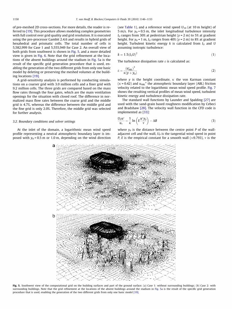
of pre-meshed 2D cross-sections. For more details, the reader is re-ferred to [19]. This procedure allows modeling complex geometrieswith full control over grid quality and grid resolution. It is executedusing the pre-processor Gambit 2.4.6 and results in hybrid grids ofhexahedral and prismatic cells. The total number of cells is5,582,999 for Case 1 and 5,555,949 for Case 2. An overall view ofboth grids from southwest is shown in Fig. 5, and a more detailedview is given in Fig. 6. Note that the grid refinement at the loca-tions of the absent buildings around the stadium in Fig. 5a is theresult of the specific grid generation procedure that is used, en-abling the generation of the two different grids from only one basicmodel by deleting or preserving the meshed volumes at the build-ing locations [19].

A grid-sensitivity analysis is performed by conducting simula-tions on a coarser grid with 3.0 million cells and a finer grid with9.2 million cells. The three grids are compared based on the massflow rates through the four gates, which are the main ventilationopenings for the situation with closed roof. The difference in nor-malized mass flow rates between the coarse grid and the middlegrid is 4.7%, whereas the difference between the middle grid andthe fine grid is only 2.0%. Therefore, the middle grid was selectedfor further analysis.

3.2. Boundary conditions and solver settings

At the inlet of the domain, a logarithmic mean wind speedprofile representing a neutral atmospheric boundary layer is im-posed with y0 = 0.5 m or 1.0 m, depending on the wind direction

Fig. 5. Southwest view of the computational grid on the building surfaces and part osurrounding buildings. Note that the grid refinement at the locations of the absent buprocedure that is used, enabling the generation of the two different grids from only one

(see Table 1), and a reference wind speed U10 (at 10 m height) of5 m/s. For y0 = 0.5 m, the inlet longitudinal turbulence intensityIU ranges from 30% at pedestrian height (y = 2 m) to 5% at gradientheight. For y0 = 1 m, IU ranges from 40% (y = 2 m) to 8% at gradientheight. Turbulent kinetic energy k is calculated from IU and Uassuming isotropic turbulence:

k ¼ 1:5ðIUUÞ2 ð1Þ

The turbulence dissipation rate e is calculated as:

e ¼ ðu�ABLÞ3

jðyþ y0Þð2Þ

where y is the height coordinate, j the von Karman constant(j = 0.42) and uABL* the atmospheric boundary layer (ABL) frictionvelocity related to the logarithmic mean wind speed profile. Fig. 7shows the resulting vertical profiles of mean wind speed, turbulentkinetic energy and turbulence dissipation rate.

The standard wall functions by Launder and Spalding [27] areused with the sand-grain based roughness modification by Cebeciand Bradshaw [28]. The velocity wall function in the CFD code isimplemented as [33]:

UPu�

us¼ 1

jln E

u�yP

m

� �� DB ð3Þ

where yP is the distance between the centre point P of the wall-adjacent cell and the wall, UP is the tangential wind speed in pointP, E is the empirical constant for a smooth wall (�9.793), m is the

f the ground surface. (a) Case 1: without surrounding buildings; (b) Case 2: withildings around the stadium in Fig. 5a is the result of the specific grid generationbasic model [19].

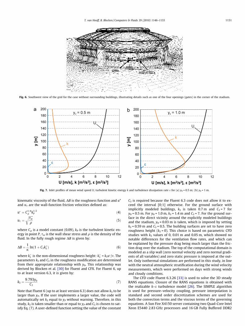
Fig. 6. Southwest view of the grid for the case without surrounding buildings, illustrating details such as one of the four openings (gates) in the corner of the stadium.

Fig. 7. Inlet profiles of mean wind speed U, turbulent kinetic energy k and turbulence dissipation rate e for (a) y0 = 0.5 m; (b) y0 = 1 m.

T. van Hooff, B. Blocken / Computers & Fluids 39 (2010) 1146–1155 1151

kinematic viscosity of the fluid, DB is the roughness function and u*and us are the wall-function friction velocities defined as:

u� ¼ C1=4l k1=2

P ð4Þ

us ¼ffiffiffiffiffiffisw

q

rð5Þ

where Cl is a model constant (0.09), kP is the turbulent kinetic en-ergy in point P, sw is the wall shear stress and q is the density of thefluid. In the fully rough regime DB is given by:

DB ¼ 1j

lnð1þ CSkþS Þ ð6Þ

where kþS is the non-dimensional roughness height: kþS = kSu�/m. Theparameters kS and CS in the roughness modification are determinedfrom their appropriate relationship with y0. This relationship wasderived by Blocken et al. [30] for Fluent and CFX. For Fluent 6, upto at least version 6.3, it is given by:

kS ¼9:793y0

CSð7Þ

Note that Fluent 6 (up to at least version 6.3) does not allow kS to belarger than yP. If the user implements a larger value, the code willautomatically set kS equal to yP without warning. Therefore, in thisstudy, kS is taken smaller than or equal to yP and CS is chosen to sat-isfy Eq. (7). A user-defined function setting the value of the constant

CS is required because the Fluent 6.3 code does not allow it to ex-ceed the interval [0;1] otherwise. For the ground surface withimplicitly modeled buildings, kS is taken 0.7 m and CS = 7 fory0 = 0.5 m. For y0 = 1.0 m, kS = 1.4 m and CS = 7. For the ground sur-face in the direct vicinity around the explicitly modeled buildingsand the stadium, y0 = 0.03 m is taken, which is imposed by settingkS = 0.59 m and CS = 0.5. The building surfaces are set to have zeroroughness height (kS = 0). This choice is based on parametric CFDstudies with kS values of 0, 0.01 m and 0.05 m, which showed nonotable differences for the ventilation flow rates, and which canbe explained by the pressure drag being much larger than the fric-tion drag over the stadium. The top of the computational domain ismodeled as a slip wall (zero normal velocity and zero normal gradi-ents of all variables) and zero static pressure is imposed at the out-let. Only isothermal simulations are performed in this study, in linewith the neutral atmospheric stratification during the wind velocitymeasurements, which were performed on days with strong windsand cloudy conditions.

The CFD code Fluent 6.3.26 [33] is used to solve the 3D steadyRANS equations. Closure of the RANS equations is obtained withthe realizable k–e turbulence model [26]. The SIMPLE algorithmis used for pressure–velocity coupling, pressure interpolation isstandard and second order discretization schemes are used forboth the convection terms and the viscous terms of the governingequations. A Sun Fire X4150 server containing two Quad-Core IntelXeon E5440 2.83 GHz processors and 16 GB Fully Buffered DDR2

1152 T. van Hooff, B. Blocken / Computers & Fluids 39 (2010) 1146–1155

memory was used to perform the simulations. Every simulationreached convergence after about 20 h of wall clock time in which6000 iterations were performed. The scaled residuals [33] reachedthe following minimum values: 10�7 for x, y and z velocity, 10�6 fork and e, and 10�5 for continuity.

4. Validation with full-scale wind velocity measurements

4.1. Measurements

For CFD validation purposes, the 3D wind velocity in andaround the stadium was measured on days with neutral atmo-spheric stratification (strong winds (reference wind speed Uref

above 8 m/s) and cloudy conditions) in the period September–November 2007. The measurements were performed with ultra-sonic anemometers, positioned on mobile posts, at 2 m heightabove the ArenA deck (Fig. 6) in the four gates which are the mainventilation openings when the roof is closed. The reference windspeed (Uref) was measured on top of a 10 m mast on the roof ofthe 95 m high ABN-AMRO office building, which is the highestbuilding in the proximity of the stadium (Fig. 3). The measurementdata were sampled at 5 Hz, averaged into 10-min values and ana-lyzed. Only data with at least 12 different 10-min values per winddirection sector of 10� were retained in order to obtain adequateaveraged wind velocities and standard deviations. The measuredwind speed U in the four gates was divided by the reference windspeed Uref measured on top of the ABN-AMRO office building. Notethat the term ‘‘wind speed” here refers to the magnitude of the 3Dmean wind velocity vector.

4.2. Comparison of measurements and CFD

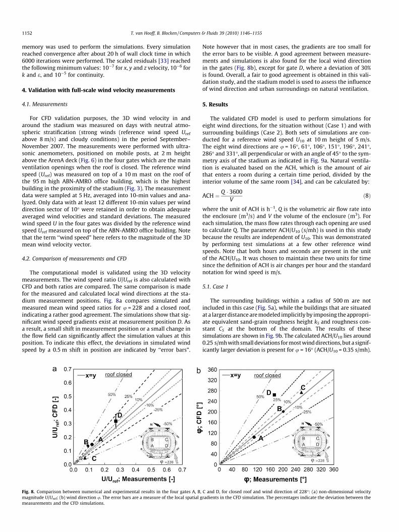
The computational model is validated using the 3D velocitymeasurements. The wind speed ratio U/Uref is also calculated withCFD and both ratios are compared. The same comparison is madefor the measured and calculated local wind directions at the sta-dium measurement positions. Fig. 8a compares simulated andmeasured mean wind speed ratios for u = 228�and a closed roof,indicating a rather good agreement. The simulations show that sig-nificant wind speed gradients exist at measurement position D. Asa result, a small shift in measurement position or a small change inthe flow field can significantly affect the simulation values at thisposition. To indicate this effect, the deviations in simulated windspeed by a 0.5 m shift in position are indicated by ‘‘error bars”.

Fig. 8. Comparison between numerical and experimental results in the four gates A, B,magnitude U/Uref; (b) wind direction u. The error bars are a measure of the local spatial gmeasurements and the CFD simulations.

Note however that in most cases, the gradients are too small forthe error bars to be visible. A good agreement between measure-ments and simulations is also found for the local wind directionin the gates (Fig. 8b), except for gate D, where a deviation of 30%is found. Overall, a fair to good agreement is obtained in this vali-dation study, and the stadium model is used to assess the influenceof wind direction and urban surroundings on natural ventilation.

5. Results

The validated CFD model is used to perform simulations foreight wind directions, for the situation without (Case 1) and withsurrounding buildings (Case 2). Both sets of simulations are con-ducted for a reference wind speed U10 at 10 m height of 5 m/s.The eight wind directions are u = 16�, 61�, 106�, 151�, 196�, 241�,286� and 331�, all perpendicular or with an angle of 45� to the sym-metry axis of the stadium as indicated in Fig. 9a. Natural ventila-tion is evaluated based on the ACH, which is the amount of airthat enters a room during a certain time period, divided by theinterior volume of the same room [34], and can be calculated by:

ACH ¼ Q � 3600V

ð8Þ

where the unit of ACH is h�1, Q is the volumetric air flow rate intothe enclosure (m3/s) and V the volume of the enclosure (m3). Foreach simulation, the mass flow rates through each opening are usedto calculate Q. The parameter ACH/U10 (s/mh) is used in this studybecause the results are independent of U10. This was demonstratedby performing test simulations at a few other reference windspeeds. Note that both hours and seconds are present in the unitof the ACH/U10. It was chosen to maintain these two units for timesince the definition of ACH is air changes per hour and the standardnotation for wind speed is m/s.

5.1. Case 1

The surrounding buildings within a radius of 500 m are notincluded in this case (Fig. 5a), while the buildings that are situatedat a larger distance are modeled implicitly by imposing the appropri-ate equivalent sand-grain roughness height kS and roughness con-stant CS at the bottom of the domain. The results of thesesimulations are shown in Fig. 9b. The calculated ACH/U10 lies around0.25 s/mh with small deviations for most wind directions, but a signif-icantly larger deviation is present for u = 16� (ACH/U10 = 0.35 s/mh).

C and D, for closed roof and wind direction of 228�: (a) non-dimensional velocityradients in the CFD simulation. The percentages indicate the deviation between the

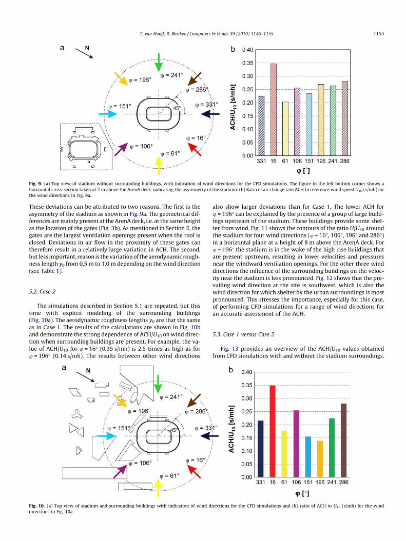
Fig. 9. (a) Top view of stadium without surrounding buildings, with indication of wind directions for the CFD simulations. The figure in the left bottom corner shows ahorizontal cross-section taken at 2 m above the ArenA deck, indicating the asymmetry of the stadium. (b) Ratio of air change rate ACH to reference wind speed U10 (s/mh) forthe wind directions in Fig. 9a.

T. van Hooff, B. Blocken / Computers & Fluids 39 (2010) 1146–1155 1153

These deviations can be attributed to two reasons. The first is theasymmetry of the stadium as shown in Fig. 9a. The geometrical dif-ferences are mainly present at the ArenA deck, i.e. at the same heightas the location of the gates (Fig. 3b). As mentioned in Section 2, thegates are the largest ventilation openings present when the roof isclosed. Deviations in air flow in the proximity of these gates cantherefore result in a relatively large variation in ACH. The second,but less important, reason is the variation of the aerodynamic rough-ness length y0 from 0.5 m to 1.0 m depending on the wind direction(see Table 1).

5.2. Case 2

The simulations described in Section 5.1 are repeated, but thistime with explicit modeling of the surrounding buildings(Fig. 10a). The aerodynamic roughness lengths y0 are that the sameas in Case 1. The results of the calculations are shown in Fig. 10band demonstrate the strong dependence of ACH/U10 on wind direc-tion when surrounding buildings are present. For example, the va-lue of ACH/U10 for u = 16� (0.35 s/mh) is 2.5 times as high as foru = 196� (0.14 s/mh). The results between other wind directions

Fig. 10. (a) Top view of stadium and surrounding buildings with indication of wind ddirections in Fig. 10a.

also show larger deviations than for Case 1. The lower ACH foru = 196� can be explained by the presence of a group of large build-ings upstream of the stadium. These buildings provide some shel-ter from wind. Fig. 11 shows the contours of the ratio U/U10 aroundthe stadium for four wind directions (u = 16�, 106�, 196� and 286�)in a horizontal plane at a height of 8 m above the ArenA deck. Foru = 196� the stadium is in the wake of the high-rise buildings thatare present upstream, resulting in lower velocities and pressuresnear the windward ventilation openings. For the other three winddirections the influence of the surrounding buildings on the veloc-ity near the stadium is less pronounced. Fig. 12 shows that the pre-vailing wind direction at the site is southwest, which is also thewind direction for which shelter by the urban surroundings is mostpronounced. This stresses the importance, especially for this case,of performing CFD simulations for a range of wind directions foran accurate assessment of the ACH.

5.3. Case 1 versus Case 2

Fig. 13 provides an overview of the ACH/U10 values obtainedfrom CFD simulations with and without the stadium surroundings.

irections for the CFD simulations and (b) ratio of ACH to U10 (s/mh) for the wind

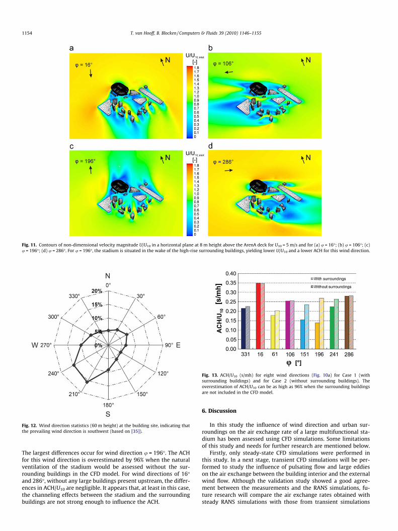
Fig. 11. Contours of non-dimensional velocity magnitude U/U10 in a horizontal plane at 8 m height above the ArenA deck for U10 = 5 m/s and for (a) u = 16�; (b) u = 106�; (c)u = 196�; (d) u = 286�. For u = 196�, the stadium is situated in the wake of the high-rise surrounding buildings, yielding lower U/U10 and a lower ACH for this wind direction.

Fig. 12. Wind direction statistics (60 m height) at the building site, indicating thatthe prevailing wind direction is southwest (based on [35]).

Fig. 13. ACH/U10 (s/mh) for eight wind directions (Fig. 10a) for Case 1 (withsurrounding buildings) and for Case 2 (without surrounding buildings). Theoverestimation of ACH/U10 can be as high as 96% when the surrounding buildingsare not included in the CFD model.

1154 T. van Hooff, B. Blocken / Computers & Fluids 39 (2010) 1146–1155

The largest differences occur for wind direction u = 196�. The ACHfor this wind direction is overestimated by 96% when the naturalventilation of the stadium would be assessed without the sur-rounding buildings in the CFD model. For wind directions of 16�and 286�, without any large buildings present upstream, the differ-ences in ACH/U10 are negligible. It appears that, at least in this case,the channeling effects between the stadium and the surroundingbuildings are not strong enough to influence the ACH.

6. Discussion

In this study the influence of wind direction and urban sur-roundings on the air exchange rate of a large multifunctional sta-dium has been assessed using CFD simulations. Some limitationsof this study and needs for further research are mentioned below.

Firstly, only steady-state CFD simulations were performed inthis study. In a next stage, transient CFD simulations will be per-formed to study the influence of pulsating flow and large eddieson the air exchange between the building interior and the externalwind flow. Although the validation study showed a good agree-ment between the measurements and the RANS simulations, fu-ture research will compare the air exchange rates obtained withsteady RANS simulations with those from transient simulations

T. van Hooff, B. Blocken / Computers & Fluids 39 (2010) 1146–1155 1155

with Large Eddy Simulation (LES) and/or Detached Eddy Simula-tion (DES). Secondly, only isothermal simulations were performedin this study, although a previous study [19] indicated the stronginfluence that local buoyancy, as a result of higher temperaturesinside the stadium compared to the ambient air temperature, canhave on the ACH. Note that both in the previous and in the currentstudy, a neutral atmospheric boundary layer was assumed. Thedecision to focus on only isothermal simulations in the presentstudy was made to limit the number of influencing parameters inorder to provide some first insights in the influence of wind direc-tion and urban surroundings on the ACH. Thermal simulationswould increase the complexity of the flow field considerably. Fur-thermore, thermal simulations would require conducting simula-tions at different reference wind speeds U10, because the ACHcannot be scaled linearly with U10 anymore. Future studies will fo-cus on the influence of wind direction and urban surroundings inthermal simulations. In general, the interaction between windand buoyancy as driving forces for natural ventilation is an impor-tant topic of future research.

7. Conclusions

A study on the influence of wind direction and urban surround-ings on natural ventilation of a large semi-enclosed stadium hasbeen presented in this paper. The 3D steady RANS CFD simulationsare performed isothermally (no buoyancy) and in a coupled way,i.e. the outdoor and the indoor air flow are solved simultaneouslyand within the same computational domain. The high-resolutionbody-fitted grid was based on a grid-sensitivity analysis, indicatingthe 5.6 million cell hybrid grid to be adequate for this study. TheCFD model was validated using on-site full-scale 3D wind velocitymeasurements in the four gates of the stadium. An overall to goodagreement was obtained between CFD simulations andmeasurements.

The natural ventilation (air change rate per hour – ACH) was as-sessed for eight wind directions and for two cases: with and with-out surrounding buildings. The results of both cases havedemonstrated the importance of performing simulations with arange of wind directions. For the isolated stadium (without sur-rounding buildings), the differences between two wind directionscan be as large as 75%. For the stadium in its urban environment,the differences between two wind directions can go up to 152%.Furthermore, this study has shown the need to model the sur-rounding urban environment for natural ventilation analysis.Excluding the urban environment in the computational domaincan lead to an overestimation of the ACH with 96%. While disre-garding surrounding buildings and focusing on only a limited num-ber of wind directions can be sufficient for isolated buildings and/or buildings in a rural environment, this can give very large errorsfor buildings in suburban and urban areas.

Acknowledgements

The measurements reported in this paper were supported bythe Laboratory of the Unit Building Physics and Systems (BPS) ofEindhoven University of Technology. Special thanks go to Ing. JanDiepens, head of LBPS, and Ing. Harrie Smulders, Wout van Bommeland GeertJan Maas, members of the LBPS, for their important con-tribution. We also thank Martin Wielaart, manager at the Amster-dam ArenA for his help during the measurements.

References

[1] Awbi HB. Ventilation of buildings. London: Spon Press; 1991.[2] Awbi HB. Design considerations for naturally ventilated buildings. Renew

Energy 1994;5:1081–90.

[3] Etheridge D, Sandberg M. Building ventilation: theory andmeasurement. Chichester, England: Wiley; 1996.

[4] Linden PF. The fluid mechanics of natural ventilation. Annu Rev Fluid Mech1999;31:201–38.

[5] Coffey CJ, Hunt GR. Ventilation effectiveness measures based on heat removal:part. 2. Application to natural ventilation flows. Build Environ2007;42(6):2249–62.

[6] Ji Y, Cook MJ, Hanby V. CFD modelling of natural displacement ventilation in anenclosure connected to an atrium. Build Environ 2007;42(3):1158–72.

[7] Straw MP, Baker CJ, Robertson AP. Experimental measurements andcomputations of the wind-induced ventilation of a cubic structure. J WindEng Ind Aerod 2000;88(2-3):213–30.

[8] Ohba M, Irie K, Kurabuchi T. Study on airflow characteristics inside and outsidea cross-ventilation model, and ventilation flow rates using wind tunnelexperiments. J Wind Eng Ind Aerod 2001;89(14-15):1513–24.

[9] Jiang Y, Alexander D, Jenkins H, Arthur R, Chen Q. Natural ventilation inbuildings: measurement in a wind tunnel and numerical simulation withlarge-eddy simulation. J Wind Eng Ind Aerod 2003;91(3):331–53.

[10] Karava P, Stathopoulos T, Athienitis AK. Wind-induced natural ventilationanalysis. Sol Energy 2007;81(1):20–30.

[11] Cook MJ, Ji Y, Hunt GR. CFD modeling of natural ventilation: combined windand buoyancy forces. Int J Vent 2003;1(3):169–80.

[12] Wright NG, Hargreaves DM. Unsteady CFD simulations for natural ventilation.Int J Vent 2006;5(1):13–20.

[13] Yang T, Wright NG, Etheridge DW, Quinn AD. A comparison of CFD and full-scale measurements for analysis of natural ventilation. Int J Vent2006;4(4):337–48.

[14] Hu C-H, Ohba M, Yoshie R. CFD modelling of unsteady cross ventilation flowsusing LES. J Wind Eng Ind Aerod 2008;96(10–11):1692–706.

[15] Horan JM, Finn DP. Sensitivity of air change rates in a naturally ventilatedatrium space subject to variations in external wind speed and direction.Energy Build 2008;40(8):1577–85.

[16] Teitel M, Ziskind G, Liran O, Dubovsky V, Letan R. Effect of wind direction ongreenhouse ventilation rate, airflow patterns and temperature distributions.Biosystems Eng 2008;101(3):351–69.

[17] Norton T, Grant J, Fallon R, Sun D-W. Assessing the ventilation effectiveness ofnaturally ventilated livestock buildings under wind dominated conditionsusing computational fluid dynamics. Biosystems Eng 2009;103(1):78–99.

[18] Jiang Y, Chen Q. Effect of fluctuating wind direction on cross naturalventilation in buildings from large eddy simulation. Build Environ2002;37(4):379–86.

[19] Van Hooff T, Blocken B. Coupled urban wind flow and indoor naturalventilation modelling on a high-resolution grid: a case study for theAmsterdam ArenA stadium. Environ Modell Softw 2010;25(1):51–65.

[20] Blocken B, Carmeliet J, Stathopoulos T. CFD evaluation of the wind speedconditions in passages between buildings – effect of wall-function roughnessmodifications on the atmospheric boundary layer flow. J Wind Eng Ind Aerod2007;95(9–11):941–62.

[21] Blocken B, Stathopoulos T, Carmeliet J. Wind environmental conditions inpassages between two long narrow perpendicular buildings. J Aerosp Eng –ASCE 2008;21(4):280–7.

[22] Blocken B, Moonen P, Stathopoulos T, Carmeliet J. A numerical study on theexistence of the Venturi-effect in passages between perpendicular buildings. JEng Mech – ASCE 2008;134(12):1021–8.

[23] Wirén BG. Effects of surrounding buildings on wind pressure distributions andventilative heat losses for a single-family house. J Wind Eng Ind Aerod1983;15(1-3):15–26.

[24] Van Moeseke G, Gratia E, Reiter S, De Herde A. Wind pressure distributioninfluence on natural ventilation for different incidences and environmentdensities. Energy Build 2005;37(8):878–89.

[25] Costola D, Blocken B, Hensen JLM. Overview of pressure coefficient data inbuilding energy simulation and airflow network programs. Build Environ2009;44(10):2027–36.

[26] Shih T-H, Liou WW, Shabbir A, Zhu J. A new k–e eddy-viscosity model for highReynolds number turbulent flows—model development and validation.Comput Fluids 1995;24(3):227–38.

[27] Launder BE, Spalding DB. The numerical computation of turbulent flows.Comput Methods Appl Mech Eng 1974;3:269–89.

[28] Cebeci T, Bradshaw P. Momentum transfer in boundary layers. HemispherePublishing Corporation; 1977.

[29] Wieringa J. Updating the Davenport roughness classification. J Wind Eng IndAerod 1992;41(1):357–68.

[30] Blocken B, Stathopoulos T, Carmeliet J. CFD simulation of the atmosphericboundary layer: wall function problems. Atmos Environ 2007;41(2):238–52.

[31] Franke J, Hellsten A, Schlünzen H, Carissimo B, editors. Best practice guidelinefor the CFD simulation of flows in the urban environment. COST OfficeBrussels; 2007.

[32] Tominaga Y, Mochida A, Yoshie R, Kataoka H, Nozu T, Yoshikawa M, et al. AIJguidelines for practical applications of CFD to pedestrian wind environmentaround buildings. J Wind Eng Ind Aerod 2008;96(10–11):1749–61.

[33] Fluent Inc.. Fluent 6.3 User’s Guide. Lebanon: Fluent Inc.; 2006.[34] ASHRAE. Handbook of Fundamentals. American Society of Heating.

Refrigerating and Air-Conditioning Engineers, Inc.: Atlanta, USA; 2005.[35] NEN. Application of mean hourly wind speed statistics for the Netherlands,

NPR 6097:2006. Dutch Practice Guideline; 2006 [in Dutch].