1-s2 0-S0266892011001032-main

Probabilistic Engineering Mechanics 29 (2012) 16–31

Contents lists available at SciVerse ScienceDirect

Probabilistic Engineering Mechanics

journal homepage: www.elsevier.com/locate/probengmech

Dimensionality reduction and visualization of structural reliability problemsusing polar featuresJorge E. Hurtado ∗

Universidad Nacional de Colombia, Apartado 127, Manizales, Colombia

a r t i c l e i n f o

Article history:Received 16 April 2011Received in revised form5 December 2011Accepted 22 December 2011Available online 30 December 2011

Keywords:Structural reliabilityReliability plotWorst case scenarioCritical realizationMonte Carlo simulation

a b s t r a c t

A method for reducing the dimensionality of a structural reliability problem of many dimensions toonly two independent dimensions is presented. Such a drastic reduction is achieved by means of apolar representation of a set of unclassified random numbers in the standard normal space. The mostimportant feature of the proposed approach is that, due to the probabilistic properties of the nonlineartransformation applied, the safe and failure classes of samples are clearly distinguishable and occupya standard position in a plot. On this basis it is possible to solve the reliability problem by means of asimple visually-aided selection of the relevant samples and discarding the rest. Also, the method permitsto identify the samples in the safe domain that are on the verge of the failure domain, which constitutethe so-called critical realizations or worst-case scenarios. Several benchmark examples demonstrate thesimplicity and versatility of the proposed approach. Finally, some classical reliabilitymethods are criticallyexamined from the point of view of the proposed reliability plot.

© 2011 Elsevier Ltd. All rights reserved.

1. Introduction

A well established definition of the reliability R of a structuralsystem is

R = 1 − Pf (1)

where Pf is the probability mass in a failure domain F of the spaceof the basic random variables x of d dimensions, determined by alimit state function g(x). This probability is defined as

Pf =

F

px(x)dx (2)

where px(x) is the joint density function of the basic variables.Evidently, the reliability corresponds to the integral evaluated inthe complementary safe domain S:

R =

S

px(x)dx. (3)

The discrimination between the two domains is done bymeansof a function of the variables g(x), which is defined in relation to alimit of the tolerable structural behavior. In solving this problem,it is common to convert it to a space u of independent Gaussian

∗ Tel.: +57 68879300; fax: +57 68879334.E-mail address: [email protected].

0266-8920/$ – see front matter© 2011 Elsevier Ltd. All rights reserved.doi:10.1016/j.probengmech.2011.12.004

variables bymeans of suitable transformations x = t(u) [1]. In thisnew space the problems reads

Pf =

F

φd(u)du (4)

where φd(u) is the standard Gaussian density function in ddimensions. The discrimination between failure and safe domainsis now determined by the transformed limit state functiong(t(u)) ≡ g(x), whichwill be denoted simply as g(u) in the sequel.

Several methods have been proposed to solve this problem.They can be grouped into two classes, namely (a) Monte Carlosimulation methods, among which are Importance Sampling[2, e.g.], Directional Simulation [e.g.] [3], Line Sampling [4],Subset Simulation [5], Radial-based Importance Sampling [6,7]and others; and (b) methods based on a functional surrogateof the limit state function either for estimating the probabilityon approximations allowed by the function as such (FORM andSORM, first- and second order reliability methods, respectively[8–10]) or for reducing the computational cost of the Monte Carlosimulation. Among the latter are Response Surfaces [11, e.g.],Neural Networks [12,13, e.g.], Support Vector Machines [14] andother techniques [15].

A source of difficulties for solving the structural reliabilityproblembymeans of anymethod is its dimensionality, determinedby the number of random variables d. In essence this is due tothe fact that the estimation of the normally very small probabilityfailure requires the detection of a few samples in high dimensionalspaces, either for building a surrogate of the limit state functionor for the Monte Carlo solution. This also makes impossible the

http://dx.doi.org/10.1016/j.probengmech.2011.12.004

http://www.elsevier.com/locate/probengmech

http://www.elsevier.com/locate/probengmech

mailto:[email protected]

http://dx.doi.org/10.1016/j.probengmech.2011.12.004

J.E. Hurtado / Probabilistic Engineering Mechanics 29 (2012) 16–31 17

visualization of the reliability problem, which is a desirable goalfor the design practice, because this would permit the selectionof relevant samples for reliability computation or for determiningthe critical realizations that constitute the so-called worst-casescenarios [16–19].

In this paper a method is proposed for reducing the dimen-sionality of the problem to only two dimensions by means of apolar representation the random samples used in a Monte Carlosimulation. In essence, the space of d dimensions is nonlinearlytransformed into a space of only two dimensions by means oftwo variables, whose probabilistic properties allow a visible dis-crimination among the safe and failure classes of samples. Such atransformation enormously facilitates the understanding and thesolution of the reliability problem, as demonstrated herein bymeans of several examples.

The paper is organized as follows. First, the significance ofthe two variables for sample clustering is exposed. Then, theirmarginal and joint probability density functions are derived. Therelationship of the reliability plot they constitute with FORMand SORM is then exposed, together with some illustrativeexamples. After this, a numerical method for computing the failureprobability from the plot is exposed. Its application is illustratedwith two structural engineering examples in which the relevanceof the plot for determining the critical realizations is highlighted.Finally, the implications of the proposed plot for the applicationof some well known structural reliability algorithms are discussedand a comparison with them in terms of computational simplicityis made. The paper ends with some conclusions.

2. The proposed approach

2.1. Dimensionality reduction

Dimensionality reduction is a common task in statisticalanalysis, especially for regression and classification purposes [20,21]. It can also be viewed either as the extraction of the mostrelevant features out of a population of a large dimensionality, or asthe compression of information, i.e. the reduction of a populationto a representative set of smaller size for transmission or storagepurposes.

A well known unsupervised learning method for achieving thisgoal is the Principal Component Analysis (PCA), which reducesthe number of random variables of interest to a few by usingthe most important eigenvalues of the covariance matrix. Moresophisticated alternatives aimed at overcoming the linearity ofstandard PCA are theKernel Principal Component Analysis [22] andthemethodof Principal Curves [23]. Other nonlinear techniques fordimensionality reduction are special kinds of Neural Networks [20]and Self-Organizing Maps [24].

A common goal of these techniques is the conversion ofthe given problem expressed in terms of the set of variablesu1, u2, . . . , ud, in which a subset of the variables possibly exhibit ahigh degree of correlation, into a problemof uncorrelated variablesv1, v2, . . . , vm, i.e.

E[vjvk] = 0, j = k, (5)

such that m < d. The absence of correlation between thenew variables is desirable because the change in one of themdoes not affect the rest. However, this is valid only in the linearsense, because statistical correlation is only a measure of lineardependence between each pair of features vj, vk and may be zerofor variables with a strong dependence, such as e.g. vj = v2

k .Only probabilistic independence assures that the variables areabsolutely uncoupled.

In addition, if the reduction can be performed down to m = 2or m = 3 without significant loss of probabilistic information,

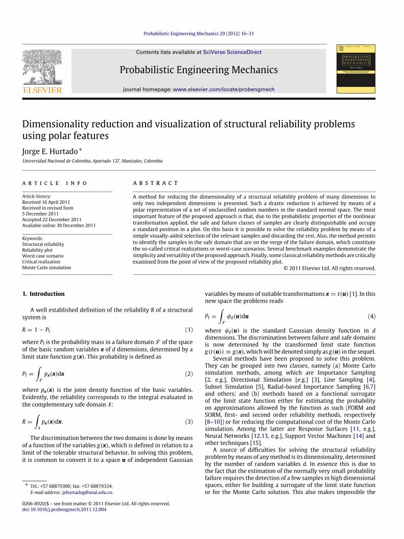
Fig. 1. The cosine as a measure of similarity between a vector ui and two vectorsof equal length and different direction. The wider the angle with ui , the larger thedifference with it.

the new problem can be rendered in a meaningful plot, which isa desirable feature indeed, as it permits the visualization of thesamples and its selection for several computations of interest.

In the context of structural reliability analysis, it is important totake into account that, if the problem has been transformed intothe standard normal space, the variables u1, u2, . . . , ud are alreadyuncorrelated and even independent, so that the application ofdimensionality reduction techniques such as the PCA is senseless.For this reason it is necessary to develop a completely differentapproach.

In this section a simple method operating a nonlineartransformation of the d-dimensional reliability problem to anew one with only m = 2 dimensions is introduced. Thetwo features are not only uncorrelated but also meet the moststringent criterion of probabilistic independence. For these andother reasons that will be clarified in the sequel, their plot makesapparent the clustering of the samples in two classes, safe andfailure. Therefore, the transformation not only makes easier thenumerical estimation of the reliability, as it permits selecting therelevant samples, but also assists the analyst for understanding theproblem in the design process in providing the critical realizations(also called worst-case scenarios [16–19]), i.e. the samples on thesafe domain that are the closest to the failure domain and in somesense determine the amplitude of the former.

2.2. Polar transformation

Let us assume that the structural reliability problem is definedin the space u of independent standard Gaussian variables and thatit is intended to solve it by means of the Monte Carlo method. Thegoal is to transform it to a problem of only two dimensions.

Consider two samples ui and uj that belong to the failuredomain. The cosine of the angle αj that separates them

cosαj = cos (ui, uj) =(ui · uj)

∥ui∥ ∥uj∥(6)

is a measure of similarity between the two vectors, as illustratedby Fig. 1. Therefore, it can be used as an indicator of the clusteringof the samples in the same class. But the length of a vector is also anindicator, because the difference between two vectors reduces as

18 J.E. Hurtado / Probabilistic Engineering Mechanics 29 (2012) 16–31

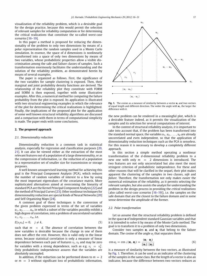
Fig. 2. The vector norm as a measure of similarity between a failure sample uiand two vectors of different lengths and equal direction. The larger the length, thesmaller the difference with ui .

their length becomes similar (see Fig. 2). This means that, takentogether, the two nonlinear features (v1, v2) = (r, cosα) mayrepresent the clustering of the samples in the two zones definedby the partitions implied by function g(u).

The nonlinear transformation for capturing the clustering of thesamples in two classes is, therefore, defined as u ∈ Rd

→ v ∈ R2

where

v1 = r =

di=1

u2i

v2 = cosα = cos (u,w) (7)

where w is the vector of the center of mass of the failure domain.It is given as

w =

F

φd(u)du−1

F

uφd(u)du

= P−1f

F

uφd(u)du. (8)

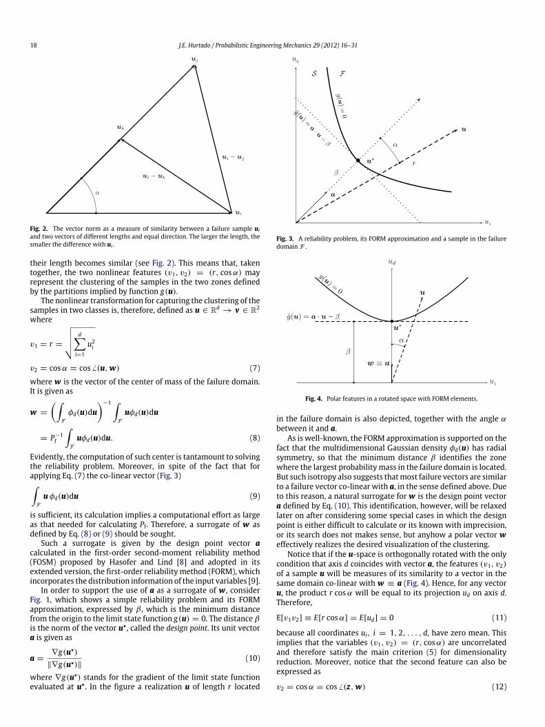
Evidently, the computation of such center is tantamount to solvingthe reliability problem. Moreover, in spite of the fact that forapplying Eq. (7) the co-linear vector (Fig. 3)

F

uφd(u)du (9)

is sufficient, its calculation implies a computational effort as largeas that needed for calculating Pf. Therefore, a surrogate of w asdefined by Eq. (8) or (9) should be sought.

Such a surrogate is given by the design point vector acalculated in the first-order second-moment reliability method(FOSM) proposed by Hasofer and Lind [8] and adopted in itsextended version, the first-order reliabilitymethod (FORM), whichincorporates the distribution information of the input variables [9].

In order to support the use of a as a surrogate of w, considerFig. 1, which shows a simple reliability problem and its FORMapproximation, expressed by β , which is the minimum distancefrom the origin to the limit state function g(u) = 0. The distance βis the norm of the vector u⋆, called the design point. Its unit vectora is given as

a =∇g(u⋆)

∥∇g(u⋆)∥(10)

where ∇g(u⋆) stands for the gradient of the limit state functionevaluated at u⋆. In the figure a realization u of length r located

Fig. 3. A reliability problem, its FORM approximation and a sample in the failuredomain F .

Fig. 4. Polar features in a rotated space with FORM elements.

in the failure domain is also depicted, together with the angle αbetween it and a.

As is well-known, the FORM approximation is supported on thefact that the multidimensional Gaussian density φd(u) has radialsymmetry, so that the minimum distance β identifies the zonewhere the largest probability mass in the failure domain is located.But such isotropy also suggests thatmost failure vectors are similarto a failure vector co-linear with a, in the sense defined above. Dueto this reason, a natural surrogate for w is the design point vectora defined by Eq. (10). This identification, however, will be relaxedlater on after considering some special cases in which the designpoint is either difficult to calculate or its known with imprecision,or its search does not makes sense, but anyhow a polar vector weffectively realizes the desired visualization of the clustering.

Notice that if the u-space is orthogonally rotated with the onlycondition that axis d coincides with vector a, the features (v1, v2)of a sample u will be measures of its similarity to a vector in thesame domain co-linear with w ≡ a (Fig. 4). Hence, for any vectoru, the product r cosα will be equal to its projection ud on axis d.Therefore,

E[v1v2] ≡ E[r cosα] = E[ud] = 0 (11)

because all coordinates ui, i = 1, 2, . . . , d, have zero mean. Thisimplies that the variables (v1, v2) = (r, cosα) are uncorrelatedand therefore satisfy the main criterion (5) for dimensionalityreduction. Moreover, notice that the second feature can also beexpressed as

v2 = cosα = cos (z,w) (12)


Fig. 5. Probability density function of the norma standardGaussian randomvector.(Dotted line: d = 2; solid line: d = 30).

where z is the unit vector in the direction of u. Since neither znor w depend on v1 = r , v2 does not either. Therefore, the twofeatures (v1, v2) are not only uncorrelated but, more importantly,independent. This is expressed as

pv1,v2(v1, v2; d) = pv1(v1; d) pv2(v2; d) (13)

where pv1(v1; d), pv2(v2; d) are the marginal probability densityfunctions of v1, v2, respectively, and pv1,v2(v1, v2; d) their jointdensity function. The number of dimensions d appears as anargument in order to emphasize the strong dependence of thesefunctions on it, as shown next.

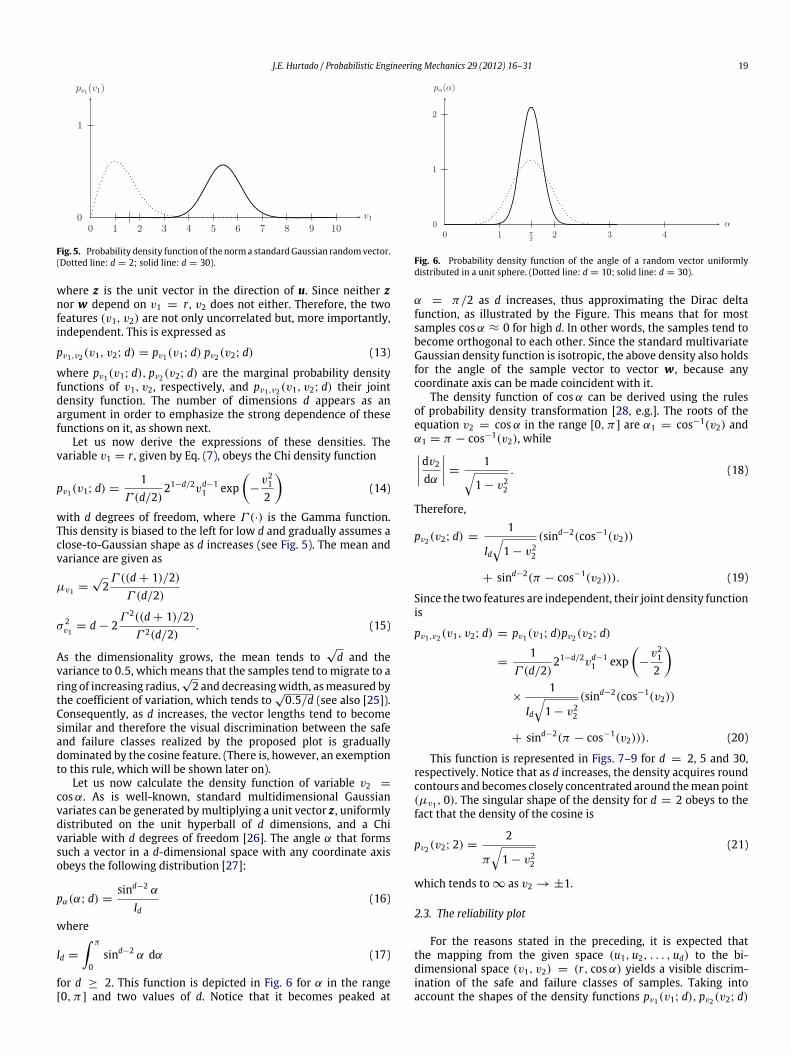
Let us now derive the expressions of these densities. Thevariable v1 = r , given by Eq. (7), obeys the Chi density function

pv1(v1; d) =1

Γ (d/2)21−d/2vd−1

1 exp

−v21

2

(14)

with d degrees of freedom, where Γ (·) is the Gamma function.This density is biased to the left for low d and gradually assumes aclose-to-Gaussian shape as d increases (see Fig. 5). The mean andvariance are given as

µv1 =√2Γ ((d + 1)/2)

Γ (d/2)

σ 2v1

= d − 2Γ 2((d + 1)/2)

Γ 2(d/2). (15)

As the dimensionality grows, the mean tends to√d and the

variance to 0.5, which means that the samples tend to migrate to aring of increasing radius,

√2 and decreasingwidth, asmeasured by

the coefficient of variation, which tends to√0.5/d (see also [25]).

Consequently, as d increases, the vector lengths tend to becomesimilar and therefore the visual discrimination between the safeand failure classes realized by the proposed plot is graduallydominated by the cosine feature. (There is, however, an exemptionto this rule, which will be shown later on).

Let us now calculate the density function of variable v2 =

cosα. As is well-known, standard multidimensional Gaussianvariates can be generated bymultiplying a unit vector z , uniformlydistributed on the unit hyperball of d dimensions, and a Chivariable with d degrees of freedom [26]. The angle α that formssuch a vector in a d-dimensional space with any coordinate axisobeys the following distribution [27]:

pα(α; d) =sind−2 α

Id(16)

where

Id =

π

0sind−2 α dα (17)

for d ≥ 2. This function is depicted in Fig. 6 for α in the range[0, π] and two values of d. Notice that it becomes peaked at

Fig. 6. Probability density function of the angle of a random vector uniformlydistributed in a unit sphere. (Dotted line: d = 10; solid line: d = 30).

α = π/2 as d increases, thus approximating the Dirac deltafunction, as illustrated by the Figure. This means that for mostsamples cosα ≈ 0 for high d. In other words, the samples tend tobecome orthogonal to each other. Since the standard multivariateGaussian density function is isotropic, the above density also holdsfor the angle of the sample vector to vector w, because anycoordinate axis can be made coincident with it.

The density function of cosα can be derived using the rulesof probability density transformation [28, e.g.]. The roots of theequation v2 = cosα in the range [0, π] are α1 = cos−1(v2) andα1 = π − cos−1(v2), whiledv2

dα

=1

1 − v22

. (18)

Therefore,

pv2(v2; d) =1

Id1 − v2

2

(sind−2(cos−1(v2))

+ sind−2(π − cos−1(v2))). (19)

Since the two features are independent, their joint density functionis

pv1,v2(v1, v2; d) = pv1(v1; d)pv2(v2; d)

=1

Γ (d/2)21−d/2vd−1

1 exp

−v21

2

×

1

Id1 − v2

2

(sind−2(cos−1(v2))

+ sind−2(π − cos−1(v2))). (20)

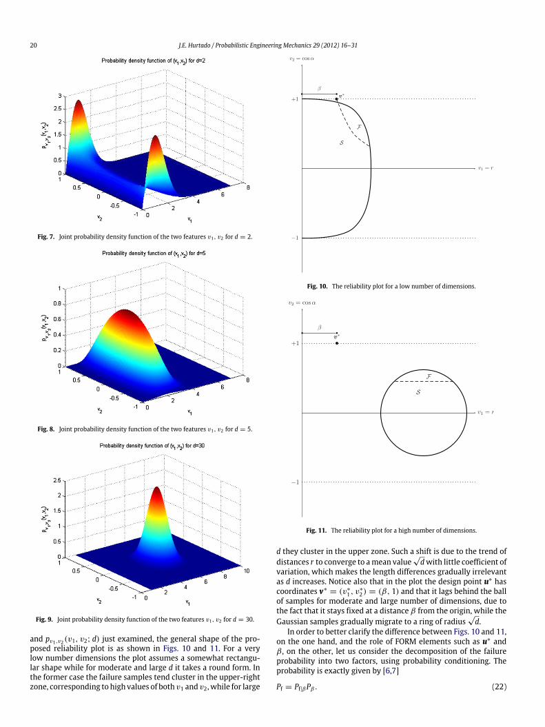
This function is represented in Figs. 7–9 for d = 2, 5 and 30,respectively. Notice that as d increases, the density acquires roundcontours and becomes closely concentrated around themean point(µv1 , 0). The singular shape of the density for d = 2 obeys to thefact that the density of the cosine is

pv2(v2; 2) =2

π

1 − v2

2

(21)

which tends to ∞ as v2 → ±1.

2.3. The reliability plot

For the reasons stated in the preceding, it is expected thatthe mapping from the given space (u1, u2, . . . , ud) to the bi-dimensional space (v1, v2) = (r, cosα) yields a visible discrim-ination of the safe and failure classes of samples. Taking intoaccount the shapes of the density functions pv1(v1; d), pv2(v2; d)


Fig. 7. Joint probability density function of the two features v1, v2 for d = 2.



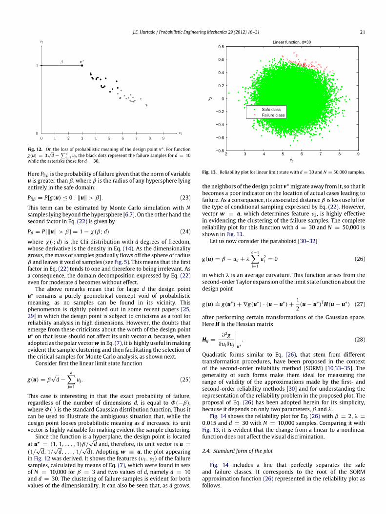
and pv1,v2(v1, v2; d) just examined, the general shape of the pro-posed reliability plot is as shown in Figs. 10 and 11. For a verylow number dimensions the plot assumes a somewhat rectangu-lar shape while for moderate and large d it takes a round form. Inthe former case the failure samples tend cluster in the upper-rightzone, corresponding to high values of both v1 and v2, while for large

Fig. 10. The reliability plot for a low number of dimensions.

Fig. 11. The reliability plot for a high number of dimensions.

d they cluster in the upper zone. Such a shift is due to the trend ofdistances r to converge to amean value

√dwith little coefficient of

variation, which makes the length differences gradually irrelevantas d increases. Notice also that in the plot the design point u∗ hascoordinates v∗

= (v∗

1 , v∗

2) = (β, 1) and that it lags behind the ballof samples for moderate and large number of dimensions, due tothe fact that it stays fixed at a distance β from the origin, while theGaussian samples gradually migrate to a ring of radius

√d.

In order to better clarify the difference between Figs. 10 and 11,on the one hand, and the role of FORM elements such as u∗ andβ , on the other, let us consider the decomposition of the failureprobability into two factors, using probability conditioning. Theprobability is exactly given by [6,7]

Pf = Pf|βPβ . (22)


Fig. 12. On the loss of probabilistic meaning of the design point v∗ . For functiong(u) = 3

√d −

dj=1 uj , the black dots represent the failure samples for d = 10

while the asterisks those for d = 30.

Here Pf|β is the probability of failure given that the normof variableu is greater than β , where β is the radius of any hypersphere lyingentirely in the safe domain:

Pf|β = P[g(u) ≤ 0 : ∥u∥ > β]. (23)

This term can be estimated by Monte Carlo simulation with Nsamples lying beyond the hypersphere [6,7]. On the other hand thesecond factor in Eq. (22) is given by

Pβ = P[∥u∥ > β] = 1 − χ(β; d) (24)

where χ(·; d) is the Chi distribution with d degrees of freedom,whose derivative is the density in Eq. (14). As the dimensionalitygrows, themass of samples gradually flows off the sphere of radiusβ and leaves it void of samples (see Fig. 5). Thismeans that the firstfactor in Eq. (22) tends to one and therefore to being irrelevant. Asa consequence, the domain decomposition expressed by Eq. (22)even for moderate d becomes without effect.

The above remarks mean that for large d the design pointu⋆ remains a purely geometrical concept void of probabilisticmeaning, as no samples can be found in its vicinity. Thisphenomenon is rightly pointed out in some recent papers [25,29] in which the design point is subject to criticisms as a tool forreliability analysis in high dimensions. However, the doubts thatemerge from these criticisms about the worth of the design pointu⋆ on that issue should not affect its unit vector a, because, whenadopted as the polar vectorw in Eq. (7), it is highly useful inmakingevident the sample clustering and then facilitating the selection ofthe critical samples for Monte Carlo analysis, as shown next.

Consider first the linear limit state function

g(u) = β√d −

dj=1

uj. (25)

This case is interesting in that the exact probability of failure,regardless of the number of dimensions d, is equal to Φ(−β),where Φ(·) is the standard Gaussian distribution function. Thus itcan be used to illustrate the ambiguous situation that, while thedesign point looses probabilistic meaning as d increases, its unitvector is highly valuable for making evident the sample clustering.

Since the function is a hyperplane, the design point is locatedat u⋆

= (1, 1, . . . , 1)β/√d and, therefore, its unit vector is a =

(1/√d, 1/

√d, . . . , 1/

√d). Adopting w ≡ a, the plot appearing

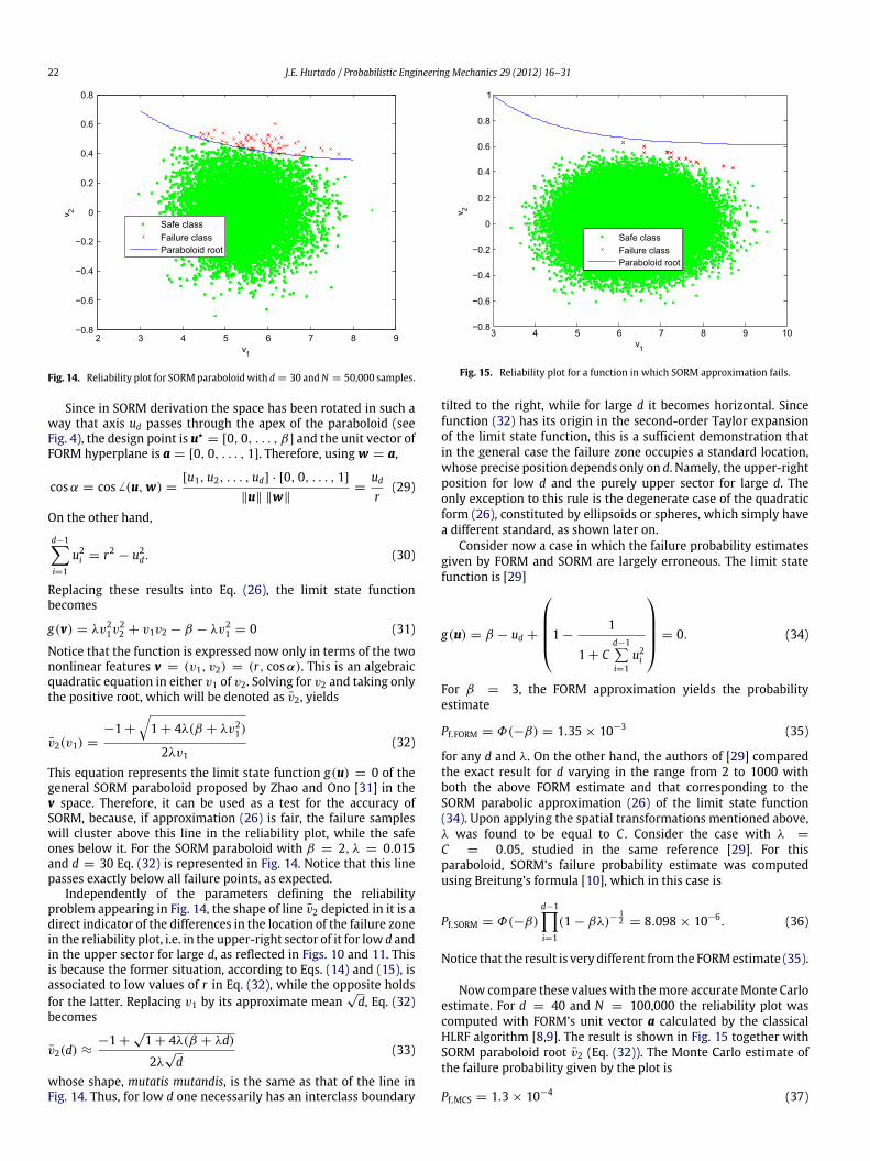
in Fig. 12 was derived. It shows the features (v1, v2) of the failuresamples, calculated by means of Eq. (7), which were found in setsof N = 10,000 for β = 3 and two values of d, namely d = 10and d = 30. The clustering of failure samples is evident for bothvalues of the dimensionality. It can also be seen that, as d grows,

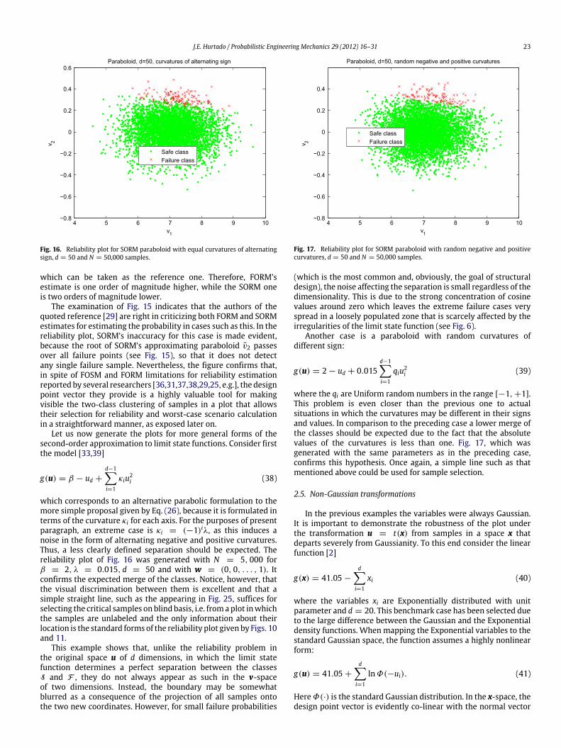
Fig. 13. Reliability plot for linear limit state with d = 30 and N = 50,000 samples.

the neighbors of the design point v∗ migrate away from it, so that itbecomes a poor indicator on the location of actual cases leading tofailure. As a consequence, its associated distance β is less useful forthe type of conditional sampling expressed by Eq. (22). However,vector w ≡ a, which determines feature v2, is highly effectivein evidencing the clustering of the failure samples. The completereliability plot for this function with d = 30 and N = 50,000 isshown in Fig. 13.

Let us now consider the paraboloid [30–32]

g(u) = β − ud + λ

d−1i=1

u2i = 0 (26)

in which λ is an average curvature. This function arises from thesecond-order Taylor expansion of the limit state function about thedesign point

g(u).= g(u∗) + ∇g(u∗) · (u − u∗) +

12(u − u∗)TH(u − u∗) (27)

after performing certain transformations of the Gaussian space.Here H is the Hessian matrix

Hij =∂2g

∂ui∂uj

u∗

. (28)

Quadratic forms similar to Eq. (26), that stem from differenttransformation procedures, have been proposed in the contextof the second-order reliability method (SORM) [10,33–35]. Thegenerality of such forms make them ideal for measuring therange of validity of the approximations made by the first- andsecond-order reliability methods [30] and for understanding therepresentation of the reliability problem in the proposed plot. Theproposal of Eq. (26) has been adopted herein for its simplicity,because it depends on only two parameters, β and λ.

Fig. 14 shows the reliability plot for Eq. (26) with β = 2, λ =

0.015 and d = 30 with N = 10,000 samples. Comparing it withFig. 13, it is evident that the change from a linear to a nonlinearfunction does not affect the visual discrimination.

2.4. Standard form of the plot

Fig. 14 includes a line that perfectly separates the safeand failure classes. It corresponds to the root of the SORMapproximation function (26) represented in the reliability plot asfollows.


Fig. 14. Reliability plot for SORMparaboloidwith d = 30 andN = 50,000 samples.

Since in SORM derivation the space has been rotated in such away that axis ud passes through the apex of the paraboloid (seeFig. 4), the design point is u⋆

= [0, 0, . . . , β] and the unit vector ofFORM hyperplane is a = [0, 0, . . . , 1]. Therefore, usingw = a,

cosα = cos (u,w) =[u1, u2, . . . , ud] · [0, 0, . . . , 1]

∥u∥ ∥w∥=

ud

r(29)

On the other hand,

d−1i=1

u2i = r2 − u2

d. (30)

Replacing these results into Eq. (26), the limit state functionbecomes

g(v) = λv21v

22 + v1v2 − β − λv2

1 = 0 (31)

Notice that the function is expressed now only in terms of the twononlinear features v = (v1, v2) = (r, cosα). This is an algebraicquadratic equation in either v1 of v2. Solving for v2 and taking onlythe positive root, which will be denoted as v2, yields

v2(v1) =

−1 +

1 + 4λ(β + λv2

1)

2λv1(32)

This equation represents the limit state function g(u) = 0 of thegeneral SORM paraboloid proposed by Zhao and Ono [31] in thev space. Therefore, it can be used as a test for the accuracy ofSORM, because, if approximation (26) is fair, the failure sampleswill cluster above this line in the reliability plot, while the safeones below it. For the SORM paraboloid with β = 2, λ = 0.015and d = 30 Eq. (32) is represented in Fig. 14. Notice that this linepasses exactly below all failure points, as expected.

Independently of the parameters defining the reliabilityproblem appearing in Fig. 14, the shape of line v2 depicted in it is adirect indicator of the differences in the location of the failure zonein the reliability plot, i.e. in the upper-right sector of it for low d andin the upper sector for large d, as reflected in Figs. 10 and 11. Thisis because the former situation, according to Eqs. (14) and (15), isassociated to low values of r in Eq. (32), while the opposite holdsfor the latter. Replacing v1 by its approximate mean

√d, Eq. (32)

becomes

v2(d) ≈−1 +

√1 + 4λ(β + λd)

2λ√d

(33)

whose shape, mutatis mutandis, is the same as that of the line inFig. 14. Thus, for low d one necessarily has an interclass boundary

Fig. 15. Reliability plot for a function in which SORM approximation fails.

tilted to the right, while for large d it becomes horizontal. Sincefunction (32) has its origin in the second-order Taylor expansionof the limit state function, this is a sufficient demonstration thatin the general case the failure zone occupies a standard location,whose precise position depends only on d. Namely, the upper-rightposition for low d and the purely upper sector for large d. Theonly exception to this rule is the degenerate case of the quadraticform (26), constituted by ellipsoids or spheres, which simply havea different standard, as shown later on.

Consider now a case in which the failure probability estimatesgiven by FORM and SORM are largely erroneous. The limit statefunction is [29]

g(u) = β − ud +

1 −1

1 + Cd−1i=1

u2i

= 0. (34)

For β = 3, the FORM approximation yields the probabilityestimate

Pf,FORM = Φ(−β) = 1.35 × 10−3 (35)

for any d and λ. On the other hand, the authors of [29] comparedthe exact result for d varying in the range from 2 to 1000 withboth the above FORM estimate and that corresponding to theSORM parabolic approximation (26) of the limit state function(34). Upon applying the spatial transformations mentioned above,λ was found to be equal to C . Consider the case with λ =

C = 0.05, studied in the same reference [29]. For thisparaboloid, SORM’s failure probability estimate was computedusing Breitung’s formula [10], which in this case is

Pf,SORM = Φ(−β)

d−1i=1

(1 − βλ)−12 = 8.098 × 10−6. (36)

Notice that the result is very different from the FORMestimate (35).

Now compare these values with themore accurateMonte Carloestimate. For d = 40 and N = 100,000 the reliability plot wascomputed with FORM’s unit vector a calculated by the classicalHLRF algorithm [8,9]. The result is shown in Fig. 15 together withSORM paraboloid root v2 (Eq. (32)). The Monte Carlo estimate ofthe failure probability given by the plot is

Pf,MCS = 1.3 × 10−4 (37)


Fig. 16. Reliability plot for SORM paraboloid with equal curvatures of alternatingsign, d = 50 and N = 50,000 samples.

which can be taken as the reference one. Therefore, FORM’sestimate is one order of magnitude higher, while the SORM oneis two orders of magnitude lower.

The examination of Fig. 15 indicates that the authors of thequoted reference [29] are right in criticizing both FORM and SORMestimates for estimating the probability in cases such as this. In thereliability plot, SORM’s inaccuracy for this case is made evident,because the root of SORM’s approximating paraboloid v2 passesover all failure points (see Fig. 15), so that it does not detectany single failure sample. Nevertheless, the figure confirms that,in spite of FOSM and FORM limitations for reliability estimationreported by several researchers [36,31,37,38,29,25, e.g.], the designpoint vector they provide is a highly valuable tool for makingvisible the two-class clustering of samples in a plot that allowstheir selection for reliability and worst-case scenario calculationin a straightforward manner, as exposed later on.

Let us now generate the plots for more general forms of thesecond-order approximation to limit state functions. Consider firstthe model [33,39]

g(u) = β − ud +

d−1i=1

κiu2i (38)

which corresponds to an alternative parabolic formulation to themore simple proposal given by Eq. (26), because it is formulated interms of the curvature κi for each axis. For the purposes of presentparagraph, an extreme case is κi = (−1)iλ, as this induces anoise in the form of alternating negative and positive curvatures.Thus, a less clearly defined separation should be expected. Thereliability plot of Fig. 16 was generated with N = 5, 000 forβ = 2, λ = 0.015, d = 50 and with w = (0, 0, . . . , 1). Itconfirms the expected merge of the classes. Notice, however, thatthe visual discrimination between them is excellent and that asimple straight line, such as the appearing in Fig. 25, suffices forselecting the critical samples onblind basis, i.e. fromaplot inwhichthe samples are unlabeled and the only information about theirlocation is the standard forms of the reliability plot given by Figs. 10and 11.

This example shows that, unlike the reliability problem inthe original space u of d dimensions, in which the limit statefunction determines a perfect separation between the classesS and F , they do not always appear as such in the v-spaceof two dimensions. Instead, the boundary may be somewhatblurred as a consequence of the projection of all samples ontothe two new coordinates. However, for small failure probabilities

Fig. 17. Reliability plot for SORM paraboloid with random negative and positivecurvatures, d = 50 and N = 50,000 samples.

(which is the most common and, obviously, the goal of structuraldesign), the noise affecting the separation is small regardless of thedimensionality. This is due to the strong concentration of cosinevalues around zero which leaves the extreme failure cases veryspread in a loosely populated zone that is scarcely affected by theirregularities of the limit state function (see Fig. 6).

Another case is a paraboloid with random curvatures ofdifferent sign:

g(u) = 2 − ud + 0.015d−1i=1

qiu2i (39)

where the qi are Uniform random numbers in the range [−1, +1].This problem is even closer than the previous one to actualsituations in which the curvatures may be different in their signsand values. In comparison to the preceding case a lower merge ofthe classes should be expected due to the fact that the absolutevalues of the curvatures is less than one. Fig. 17, which wasgenerated with the same parameters as in the preceding case,confirms this hypothesis. Once again, a simple line such as thatmentioned above could be used for sample selection.

2.5. Non-Gaussian transformations

In the previous examples the variables were always Gaussian.It is important to demonstrate the robustness of the plot underthe transformation u = t(x) from samples in a space x thatdeparts severely from Gaussianity. To this end consider the linearfunction [2]

g(x) = 41.05 −

di=1

xi (40)

where the variables xi are Exponentially distributed with unitparameter and d = 20. This benchmark case has been selected dueto the large difference between the Gaussian and the Exponentialdensity functions. When mapping the Exponential variables to thestandard Gaussian space, the function assumes a highly nonlinearform:

g(u) = 41.05 +

di=1

lnΦ(−ui). (41)

HereΦ(·) is the standard Gaussian distribution. In the x-space, thedesign point vector is evidently co-linear with the normal vector


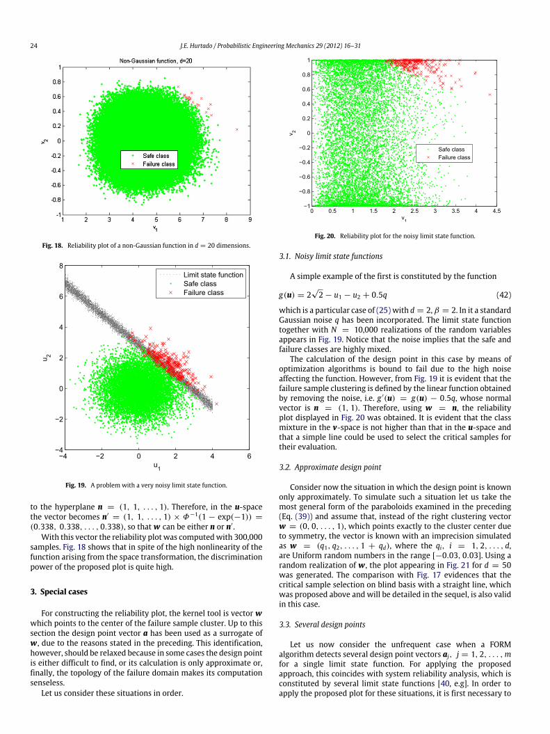
Fig. 18. Reliability plot of a non-Gaussian function in d = 20 dimensions.

Fig. 19. A problem with a very noisy limit state function.

to the hyperplane n = (1, 1, . . . , 1). Therefore, in the u-spacethe vector becomes n′

= (1, 1, . . . , 1) × Φ−1(1 − exp(−1)) =

(0.338, 0.338, . . . , 0.338), so thatw can be either n or n′.With this vector the reliability plot was computedwith 300,000

samples. Fig. 18 shows that in spite of the high nonlinearity of thefunction arising from the space transformation, the discriminationpower of the proposed plot is quite high.

3. Special cases

For constructing the reliability plot, the kernel tool is vector wwhich points to the center of the failure sample cluster. Up to thissection the design point vector a has been used as a surrogate ofw, due to the reasons stated in the preceding. This identification,however, should be relaxed because in some cases the design pointis either difficult to find, or its calculation is only approximate or,finally, the topology of the failure domain makes its computationsenseless.

Let us consider these situations in order.

Fig. 20. Reliability plot for the noisy limit state function.

3.1. Noisy limit state functions

A simple example of the first is constituted by the function

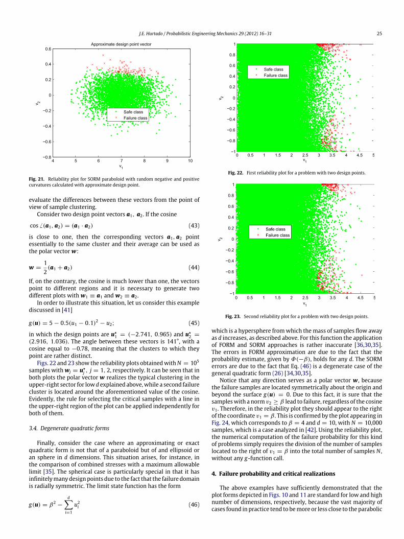
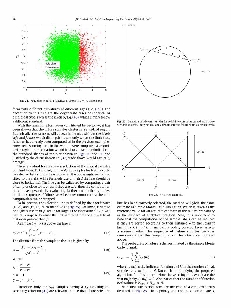
g(u) = 2√2 − u1 − u2 + 0.5q (42)

which is a particular case of (25) with d = 2, β = 2. In it a standardGaussian noise q has been incorporated. The limit state functiontogether with N = 10,000 realizations of the random variablesappears in Fig. 19. Notice that the noise implies that the safe andfailure classes are highly mixed.

The calculation of the design point in this case by means ofoptimization algorithms is bound to fail due to the high noiseaffecting the function. However, from Fig. 19 it is evident that thefailure sample clustering is defined by the linear function obtainedby removing the noise, i.e. g ′(u) = g(u) − 0.5q, whose normalvector is n = (1, 1). Therefore, using w = n, the reliabilityplot displayed in Fig. 20 was obtained. It is evident that the classmixture in the v-space is not higher than that in the u-space andthat a simple line could be used to select the critical samples fortheir evaluation.

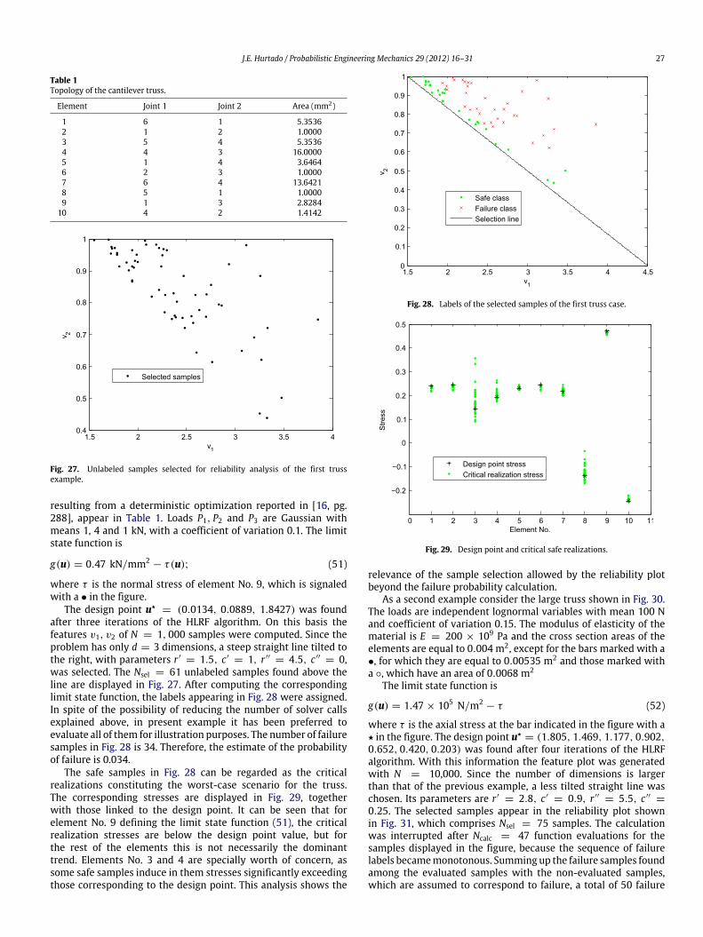
3.2. Approximate design point

Consider now the situation in which the design point is knownonly approximately. To simulate such a situation let us take themost general form of the paraboloids examined in the preceding(Eq. (39)) and assume that, instead of the right clustering vectorw = (0, 0, . . . , 1), which points exactly to the cluster center dueto symmetry, the vector is known with an imprecision simulatedas w = (q1, q2, . . . , 1 + qd), where the qi, i = 1, 2, . . . , d,are Uniform random numbers in the range [−0.03, 0.03]. Using arandom realization of w, the plot appearing in Fig. 21 for d = 50was generated. The comparison with Fig. 17 evidences that thecritical sample selection on blind basis with a straight line, whichwas proposed above and will be detailed in the sequel, is also validin this case.

3.3. Several design points

Let us now consider the unfrequent case when a FORMalgorithm detects several design point vectors aj, j = 1, 2, . . . ,mfor a single limit state function. For applying the proposedapproach, this coincides with system reliability analysis, which isconstituted by several limit state functions [40, e.g]. In order toapply the proposed plot for these situations, it is first necessary to


Fig. 21. Reliability plot for SORM paraboloid with random negative and positivecurvatures calculated with approximate design point.

evaluate the differences between these vectors from the point ofview of sample clustering.

Consider two design point vectors a1, a2. If the cosine

cos (a1, a2) = (a1 · a2) (43)

is close to one, then the corresponding vectors a1, a2 pointessentially to the same cluster and their average can be used asthe polar vectorw:

w =12(a1 + a2) (44)

If, on the contrary, the cosine is much lower than one, the vectorspoint to different regions and it is necessary to generate twodifferent plots withw1 ≡ a1 andw2 ≡ a2.

In order to illustrate this situation, let us consider this examplediscussed in [41]

g(u) = 5 − 0.5(u1 − 0.1)2 − u2; (45)

in which the design points are u⋆1 = (−2.741, 0.965) and u⋆

2 =

(2.916, 1.036). The angle between these vectors is 141°, with acosine equal to −0.78, meaning that the clusters to which theypoint are rather distinct.

Figs. 22 and 23 show the reliability plots obtainedwithN = 105

samples withwj = u⋆j , j = 1, 2, respectively. It can be seen that in

both plots the polar vector w realizes the typical clustering in theupper-right sector for low d explained above,while a second failurecluster is located around the aforementioned value of the cosine.Evidently, the rule for selecting the critical samples with a line inthe upper-right region of the plot can be applied independently forboth of them.

3.4. Degenerate quadratic forms

Finally, consider the case where an approximating or exactquadratic form is not that of a paraboloid but of and ellipsoid oran sphere in d dimensions. This situation arises, for instance, inthe comparison of combined stresses with a maximum allowablelimit [35]. The spherical case is particularly special in that it hasinfinitelymanydesignpoints due to the fact that the failure domainis radially symmetric. The limit state function has the form

g(u) = β2−

di=1

u2i (46)

Fig. 22. First reliability plot for a problem with two design points.

Fig. 23. Second reliability plot for a problem with two design points.

which is a hypersphere fromwhich themass of samples flow awayas d increases, as described above. For this function the applicationof FORM and SORM approaches is rather inaccurate [36,30,35].The errors in FORM approximation are due to the fact that theprobability estimate, given by Φ(−β), holds for any d. The SORMerrors are due to the fact that Eq. (46) is a degenerate case of thegeneral quadratic form (26) [34,30,35].

Notice that any direction serves as a polar vector w, becausethe failure samples are located symmetrically about the origin andbeyond the surface g(u) = 0. Due to this fact, it is sure that thesampleswith a norm v2 ≥ β lead to failure, regardless of the cosinev1. Therefore, in the reliability plot they should appear to the rightof the coordinate v1 = β . This is confirmed by the plot appearing inFig. 24, which corresponds to β = 4 and d = 10, with N = 10,000samples, which is a case analyzed in [42]. Using the reliability plot,the numerical computation of the failure probability for this kindof problems simply requires the division of the number of sampleslocated to the right of v1 = β into the total number of samples N ,without any g-function call.

4. Failure probability and critical realizations

The above examples have sufficiently demonstrated that theplot forms depicted in Figs. 10 and 11 are standard for low and highnumber of dimensions, respectively, because the vast majority ofcases found in practice tend to bemore or less close to the parabolic


Fig. 24. Reliability plot for a spherical problem in d = 10 dimensions.

form with different curvatures of different signs (Eq. (39)). Theexception to this rule are the degenerate cases of spherical orellipsoidal type, such as the given by Eq. (46), which simply followa different standard.

With the minimal information constituted by vector w, it hasbeen shown that the failure samples cluster in a standard region.But, initially, the samples will appear in the plot without the labelssafe and failure which distinguish them only when the limit statefunction has already been computed, as in the previous examples.However, assuming that, in the event it were computed, a second-order Taylor approximation would lead to a quasi-parabolic form,the standard shapes of the plot shown in Figs. 10 and 11, andjustified by the discussion on Eq. (32)made above, would naturallyemerge.

These standard forms allow a selection of the critical sampleson blind basis. To this end, for low d, the samples for testing couldbe selected by a straight line located in the upper-right sector andtilted to the right, while for moderate or high d the line should beclose to horizontal. The line can be validated by computing a pairof samples close to its ends; if they are safe, then the computationmay move upwards by evaluating farther and farther samples,until the sequence of failure cases becomes monotonous; then thecomputation can be stopped.

To be precise, the selection line is defined by the coordinates(r ′, c ′) and (r ′′, c ′′), such that r ′ < r ′′ (Fig. 25). For low d, r ′ shouldbe slightly less than β , while for large d the inequality r ′ > β willnaturally impose, because the first samples from the left will be atdistances greater than β .

A sample (v1, v2) is above the line if

v2 ≥ c ′′+

c ′− c ′′

r ′ − r ′′(v1 − r ′′). (47)

The distance from the sample to the line is given by

ρ =|Av1 + Bv2 + C |

√A2 + B2

; (48)

where

A =c ′

− c ′′

r ′ − r ′′

B = −1

C = c ′′− Ar ′′.

(49)

Therefore, only the Nsel samples having a v2 matching thescreening criterion (47) are relevant. Notice that, if the selection

Fig. 25. Selection of relevant samples for reliability computation and worst-casescenario analysis. The symbols and • denote safe and failure samples, respectively.

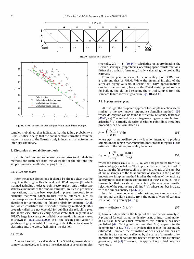
Fig. 26. First truss example.

line has been correctly selected, the method will yield the sameestimate as simple Monte Carlo simulation, which is taken as thereference value for an accurate estimate of the failure probabilityin the absence of analytical solution. Also, it is important tonote that the computation of the sample labels can be reducedif they are sorted according to their distance ρ to the straightline (r ′, c ′), (r ′′, c ′′), in increasing order, because there arrivesa moment when the sequence of failure samples becomesmonotonous and the computation can be interrupted, as saidabove.

The probability of failure is then estimated by the simpleMonteCarlo formula

Pf,MCS =1N

Ni=1

IF (ui) (50)

where IF (ui) is the indicator function and N is the number of i.i.d.samples ui, i = 1, . . . ,N . Notice that, in applying the proposedalgorithm, for all samples below the selecting line, which are thevast majority, IF (ui) = 0. Also notice that the number of functionevaluations is Ncalc < Nsel ≪ N .

As a first illustration, consider the case of a cantilever trussdepicted in Fig. 26. The topology and the cross section areas,


Table 1Topology of the cantilever truss.

Element Joint 1 Joint 2 Area (mm2)

1 6 1 5.35362 1 2 1.00003 5 4 5.35364 4 3 16.00005 1 4 3.64646 2 3 1.00007 6 4 13.64218 5 1 1.00009 1 3 2.8284

10 4 2 1.4142

Fig. 27. Unlabeled samples selected for reliability analysis of the first trussexample.

resulting from a deterministic optimization reported in [16, pg.288], appear in Table 1. Loads P1, P2 and P3 are Gaussian withmeans 1, 4 and 1 kN, with a coefficient of variation 0.1. The limitstate function is

g(u) = 0.47 kN/mm2− τ(u); (51)

where τ is the normal stress of element No. 9, which is signaledwith a • in the figure.

The design point u⋆= (0.0134, 0.0889, 1.8427) was found

after three iterations of the HLRF algorithm. On this basis thefeatures v1, v2 of N = 1, 000 samples were computed. Since theproblem has only d = 3 dimensions, a steep straight line tilted tothe right, with parameters r ′

= 1.5, c ′= 1, r ′′

= 4.5, c ′′= 0,

was selected. The Nsel = 61 unlabeled samples found above theline are displayed in Fig. 27. After computing the correspondinglimit state function, the labels appearing in Fig. 28 were assigned.In spite of the possibility of reducing the number of solver callsexplained above, in present example it has been preferred toevaluate all of them for illustration purposes. The number of failuresamples in Fig. 28 is 34. Therefore, the estimate of the probabilityof failure is 0.034.

The safe samples in Fig. 28 can be regarded as the criticalrealizations constituting the worst-case scenario for the truss.The corresponding stresses are displayed in Fig. 29, togetherwith those linked to the design point. It can be seen that forelement No. 9 defining the limit state function (51), the criticalrealization stresses are below the design point value, but forthe rest of the elements this is not necessarily the dominanttrend. Elements No. 3 and 4 are specially worth of concern, assome safe samples induce in them stresses significantly exceedingthose corresponding to the design point. This analysis shows the

Fig. 28. Labels of the selected samples of the first truss case.

Fig. 29. Design point and critical safe realizations.

relevance of the sample selection allowed by the reliability plotbeyond the failure probability calculation.

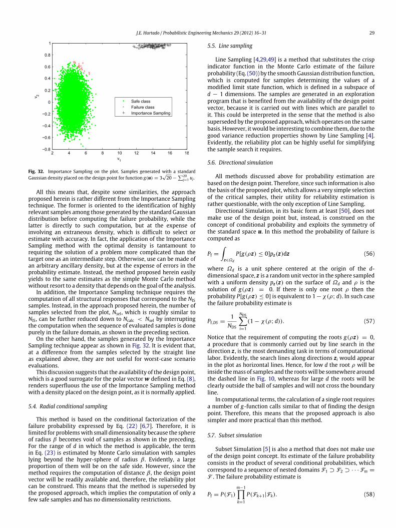
As a second example consider the large truss shown in Fig. 30.The loads are independent lognormal variables with mean 100 Nand coefficient of variation 0.15. The modulus of elasticity of thematerial is E = 200 × 109 Pa and the cross section areas of theelements are equal to 0.004 m2, except for the bars marked with a•, for which they are equal to 0.00535 m2 and those marked witha , which have an area of 0.0068 m2

The limit state function is

g(u) = 1.47 × 105 N/m2− τ (52)

where τ is the axial stress at the bar indicated in the figure with a⋆ in the figure. The design point u⋆

= (1.805, 1.469, 1.177, 0.902,0.652, 0.420, 0.203) was found after four iterations of the HLRFalgorithm. With this information the feature plot was generatedwith N = 10,000. Since the number of dimensions is largerthan that of the previous example, a less tilted straight line waschosen. Its parameters are r ′

= 2.8, c ′= 0.9, r ′′

= 5.5, c ′′=

0.25. The selected samples appear in the reliability plot shownin Fig. 31, which comprises Nsel = 75 samples. The calculationwas interrupted after Ncalc = 47 function evaluations for thesamples displayed in the figure, because the sequence of failurelabels becamemonotonous. Summing up the failure samples foundamong the evaluated samples with the non-evaluated samples,which are assumed to correspond to failure, a total of 50 failure


Fig. 30. Second truss example.

Fig. 31. Labels of the calculated samples for the second truss example.

samples is obtained, thus indicating that the failure probability is0.0050. Notice, finally, that the nonlinear transformation from thelognormal space to the Gaussian only induces a small noise in theinter-class boundary.

5. Discussion on reliability methods

In this final section some well known structural reliabilitymethods are examined from the viewpoint of the plot and thesimple numerical method emerging from it.

5.1. FOSM and FORM

After the above discussions, it should be already clear that theinsights in the original Hasofer and Lind FOSM proposal [8], whichis aimed at finding the design point vector a given only the first twostatistical moments of the random variables, are rich in geometricimplications, that have been exploited in present proposal. Someelements that were added to that original approach, such asthe incorporation of non-Gaussian probability information in thealgorithm for computing the failure probability estimate [9,43],and which constitute the first-order reliability method (FORM)properly called, are not essential for building the reliability plot.The above case studies clearly demonstrate that, regardless ofFORM’s large inaccuracy for reliability estimation in many cases,as shown in [36,31,37,38,29,25, e.g.], the design point vector ityields are highly valuable for making evident the critical sampleclustering and, therefore, facilitating its selection.

5.2. SORM

As is well known, the calculation of the SORM approximation issomewhat involved, as it needs the calculation of several samples

(typically, 2(d − 1) [30,44]), calculating or approximating theHessian, solving eigenproblems, operating space transformations,fitting the quadratic form and, finally, calculating the probabilityestimate.

From the point of view of the reliability plot, SORM caseis different that of FORM. While the essential insights of thelatter are highly valuable, it seems that SORM approximationscan be dispensed with, because the FORM design point sufficesfor building the plot and selecting the critical samples from thestandard failure sectors signaled in Figs. 10 and 11.

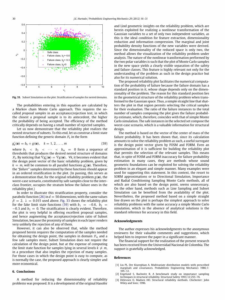
5.3. Importance sampling

At first sight the proposed approach for sample selection seemssimilar to the well-known Importance Sampling method [45],whose description can be found in structural reliability textbooks[46,40, e.g]. The method consists in generating some samples fromadensityh(u)normally placedon thedesignpoint. Since the failureprobability can be formulated as

Pf =

F

φd(u)

h(u)h(u)du (53)

where h(x) is an auxiliary density function intended to producesamples in the region that contributes most to the integral (4), theestimate of the failure probability becomes:

Pf,IS =1NIS

NISi=1

IF (ui)φd(ui)

h(ui)(54)

where the samples ui, i = 1, . . . ,NIS are now generated from h(u)instead of φd(u) as before. The important issue is that, instead ofevaluating the failure probability simply as the ratio of the numberof failure samples to the total number of samples in the plot, theImportance Sampling method implies the values of the ancillarydensity function h(u) in the computation of the Pf estimate. This inturn implies that the estimate is affected by the arbitrariness in theselection of the parameters defining h(u), whose number increasewith the dimensionality d [2,47,38].

In order to overcome such arbitrariness, use can be made ofthe optimal ancillary density from the point of view of variancereduction. It is given by [46, e.g]

h(u) =1PfI[g(u) ≤ 0]φd(u). (55)

It, however, depends on the target of the calculation, namely Pf.A proposal for estimating the density using a linear combinationof Gaussian functions that overcomes this difficulty has beenpublished [42]. Taking into account that h(u) appears in thedenominator of Eq. (54), it is evident that it must be accuratelyestimated. However, the estimation of densities on the basis ofsamples is a task seriously affected by the curse of dimensionality,because the number of samples needed for its accurate estimationgrows very fast [48]. Therefore, this approach is justified only for avery low d.


Fig. 32. Importance Sampling on the plot. Samples generated with a standardGaussian density placed on the design point for function g(u) = 3

√20 −

20j=1 uj .

All this means that, despite some similarities, the approachproposed herein is rather different from the Importance Samplingtechnique. The former is oriented to the identification of highlyrelevant samples among those generated by the standard Gaussiandistribution before computing the failure probability, while thelatter is directly to such computation, but at the expense ofinvolving an extraneous density, which is difficult to select orestimate with accuracy. In fact, the application of the ImportanceSampling method with the optimal density is tantamount torequiring the solution of a problem more complicated than thetarget one as an intermediate step. Otherwise, use can be made ofan arbitrary ancillary density, but at the expense of errors in theprobability estimate. Instead, the method proposed herein easilyyields to the same estimates as the simple Monte Carlo methodwithout resort to a density that depends on the goal of the analysis.

In addition, the Importance Sampling technique requires thecomputation of all structural responses that correspond to the NISsamples. Instead, in the approach proposed herein, the number ofsamples selected from the plot, Nsel, which is roughly similar toNIS, can be further reduced down to Ncalc < Nsel by interruptingthe computation when the sequence of evaluated samples is donepurely in the failure domain, as shown in the preceding section.

On the other hand, the samples generated by the ImportanceSampling technique appear as shown in Fig. 32. It is evident that,at a difference from the samples selected by the straight lineas explained above, they are not useful for worst-case scenarioevaluations.

This discussion suggests that the availability of the design point,which is a good surrogate for the polar vectorw defined in Eq. (8),renders superfluous the use of the Importance Sampling methodwith a density placed on the design point, as it is normally applied.

5.4. Radial conditional sampling

This method is based on the conditional factorization of thefailure probability expressed by Eq. (22) [6,7]. Therefore, it islimited for problemswith small dimensionality because the sphereof radius β becomes void of samples as shown in the preceding.For the range of d in which the method is applicable, the termin Eq. (23) is estimated by Monte Carlo simulation with sampleslying beyond the hyper-sphere of radius β . Evidently, a largeproportion of them will be on the safe side. However, since themethod requires the computation of distance β , the design pointvector will be readily available and, therefore, the reliability plotcan be construed. This means that the method is superseded bythe proposed approach, which implies the computation of only afew safe samples and has no dimensionality restrictions.

5.5. Line sampling

Line Sampling [4,29,49] is a method that substitutes the crispindicator function in the Monte Carlo estimate of the failureprobability (Eq. (50)) by the smoothGaussian distribution function,which is computed for samples determining the values of amodified limit state function, which is defined in a subspace ofd − 1 dimensions. The samples are generated in an explorationprogram that is benefited from the availability of the design pointvector, because it is carried out with lines which are parallel toit. This could be interpreted in the sense that the method is alsosuperseded by the proposed approach,which operates on the samebasis. However, itwould be interesting to combine them, due to thegood variance reduction properties shown by Line Sampling [4].Evidently, the reliability plot can be highly useful for simplifyingthe sample search it requires.

5.6. Directional simulation

All methods discussed above for probability estimation arebased on the design point. Therefore, since such information is alsothe basis of the proposed plot, which allows a very simple selectionof the critical samples, their utility for reliability estimation israther questionable, with the only exception of Line Sampling.

Directional Simulation, in its basic form at least [50], does notmake use of the design point but, instead, is construed on theconcept of conditional probability and exploits the symmetry ofthe standard space u. In this method the probability of failure iscomputed as

Pf =

z∈Ωd

P[g(ρz) ≤ 0]pz(z)dz (56)

where Ωd is a unit sphere centered at the origin of the d-dimensional space, z is a randomunit vector in the sphere sampledwith a uniform density pz(z) on the surface of Ωd and ρ is thesolution of g(ρz) = 0. If there is only one root ρ then theprobability P[g(ρz) ≤ 0] is equivalent to 1−χ(ρ; d). In such casethe failure probability estimate is

Pf,DS =1

NDS

NDSi=1

(1 − χ(ρ; d)). (57)

Notice that the requirement of computing the roots g(ρz) = 0,a procedure that is commonly carried out by line search in thedirection z , is the most demanding task in terms of computationallabor. Evidently, the search lines along directions zi would appearin the plot as horizontal lines. Hence, for low d the root ρ will beinside themass of samples and the rootswill be somewhere aroundthe dashed line in Fig. 10, whereas for large d the roots will beclearly outside the ball of samples and will not cross the boundaryline.

In computational terms, the calculation of a single root requiresa number of g-function calls similar to that of finding the designpoint. Therefore, this means that the proposed approach is alsosimpler and more practical than this method.

5.7. Subset simulation

Subset Simulation [5] is also a method that does not make useof the design point concept. Its estimate of the failure probabilityconsists in the product of several conditional probabilities, whichcorrespond to a sequence of nested domains F1 ⊃ F2 ⊃ · · · Fm =

F . The failure probability estimate is

Pf = P(F1)

m−1k=1

P(Fk+1|Fk). (58)


Fig. 33. Subset Simulation on the plot. Stratification of samples for nested domains.

The probabilities entering in this equation are calculated bya Markov chain Monte Carlo approach. This requires the so-called proposal samples in an acceptance/rejection test, in whichthe closest a proposal sample is to its antecedent, the higherthe probability of being accepted. The efficiency of the methodcritically depends on having a small number of rejected samples.

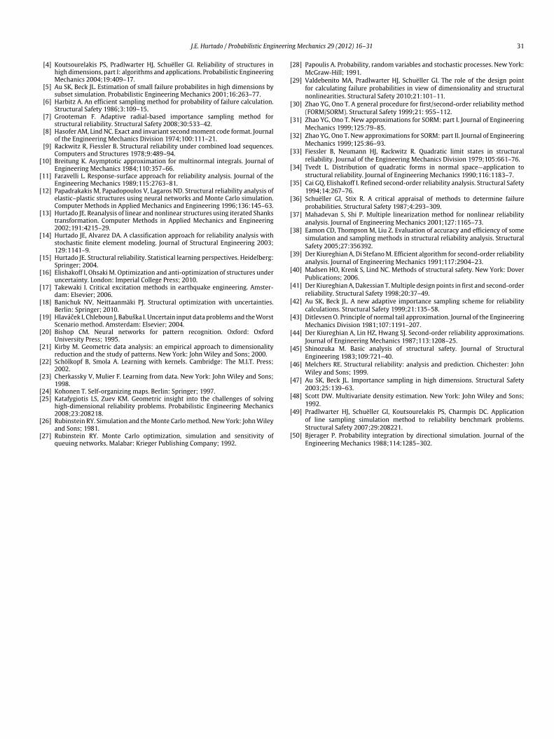
Let us now demonstrate that the reliability plot realizes thenested structure of subsets. To this end, let us construe a limit statefunction defining the generic domain Fk in the form

g ′

k(u) = bk + g(u), k = 1, 2, . . . ,m (59)

where b1 < b2 < · · · < bm = 0 form a sequence ofthresholds that produces the desired nested structure of domainsFk. By noticing that ∇g ′

k(u) = ∇g(u), ∀k, it becomes evident thatthe design point vector of the basic reliability problem, given byk = m, will be common to all parallel functions g ′

k(u). Therefore,the ‘‘failure’’ samples determined by these functions should appearin an ordered stratification in the plot. (In passing, this serves asa demonstration that, for the original reliability problem g(u), theworst-case scenario, constituted by safe samples close to the inter-class frontier, occupies the stratum below the failure ones in thereliability plot.)

In order to illustrate this stratification property, consider theparabolic function (26) in d = 50dimensions,with the samevaluesβ = 2, λ = 0.015 used above. Fig. 33 shows the reliability plotfor the fake limit state functions (59) with b1 = −0.6, b2 =

−0.3 and b3 = 0. The stratification is clearly evident. Therefore,the plot is very helpful in offering excellent proposal samples,and hence augmenting the acceptance/rejection ratio of SubsetSimulation, because the proximity of samples in each layer rendersvery unlikely the rejection of any of them.

However, it can also be observed that, while the methodproposed herein requires the computation of the samples neededfor obtaining the design point, the samples in domain Fm and afew safe samples more, Subset Simulation does not require thecalculation of the design point, but at the expense of computingthe limit state function for samples lying in several levels k = m,in a procedure that also implies the rejection of many samples.For those cases in which the design point is easy to compute, asis normally the case, the proposed approach is clearly simpler andmore economical.

6. Conclusions

A method for reducing the dimensionality of reliabilityproblemswas proposed. It is a development of the original Hasofer

and Lind geometric insights on the reliability problem, which areherein exploited for realizing a nonlinear transformation of theGaussian variables to a set of only two independent variables, asthis is the ideal condition for feature extraction, dimensionalityreduction and information compression. The marginal and jointprobability density functions of the new variables were derived.Since the dimensionality of the reduced space is only two, themethod allows the visualization of the reliability problem underanalysis. The nature of the nonlinear transformation performed bythe two polar variables is such that the plot ofMonte Carlo samplesin the new space yields a clearly visible separation of the safetyand failure classes. This feature is highly relevant not only for theunderstanding of the problem as such in the design practice butalso for its numerical solution.

The proposed reliability plot facilitates the numerical computa-tion of the probability of failure because the failure domain has astandard position in it, whose shape depends only on the dimen-sionality of the problem. The reason for this standard position liesin the geometrical structure of the reliability problemwhen trans-formed to theGaussian space. Thus, a simple straight line that shat-ters the plot in that region permits selecting the critical samplesfor their evaluation. The ratio of the failure instances to the totalnumber of samples composing the plot gives the failure probabil-ity estimate, which, therefore, coincides with that of simple MonteCarlo simulation. The safe instances in the selected set compose theworst-case scenario, which is a valuable information for structuraldesign.

The method is based on the vector of the center of mass of thefailure probability. It has been shown that, since its calculationamounts to solve the reliability problem as such, a useful surrogateis the design point vector given by FOSM and FORM. Even anapproximation of it is sufficient for building the reliability plotthat permits the selection of the relevant samples. This meansthat, in spite of FOSM and FORM inaccuracy for failure probabilityestimation in many cases, they are methods whose soundgeometric foundations can be exploited for solving the reliabilityproblem in an elegant and simple manner. Many examples wereused for supporting this statement. In this context, the resort toSORM approximations or to Directional Simulation, Importanceand Radial Conditioning Sampling Monte Carlo methods, all ofwhich are also based on the design point, seems unnecessary.On the other hand, methods such as Line Sampling and SubsetSimulation can be benefited from the availability of the plot.Nevertheless, the proposed method based on a simple straightline drawn on the plot is perhaps the simplest approach to solvereliability problems with the same accuracy a simple Monte Carlosimulation, which in the absence of analytical solutions is thestandard reference for accuracy in this field.

Acknowledgments

The author expresses his acknowledgments to the anonymousreviewers for their valuable comments and suggestions, whichhelped him to improve the paper in a significant manner.

The financial support for the realization of the present researchhas been received from the Universidad Nacional de Colombia. Thesupport is gratefully acknowledged.

References

[1] Liu PL, Der Kiureghian A. Multivariate distribution models with prescribedmarginals and covariances. Probabilistic Engineering Mechanics 1986;1:105–12.

[2] Engelund S, Rackwitz R. A benchmark study on importance samplingtechniques in structural reliability. Structural Safety 1993;12:255–76.

[3] Ditlevsen O, Madsen HO. Structural reliability methods. Chichester: JohnWiley and Sons; 1996.


[4] Koutsourelakis PS, Pradlwarter HJ, Schuëller GI. Reliability of structures inhigh dimensions, part I: algorithms and applications. Probabilistic EngineeringMechanics 2004;19:409–17.

[5] Au SK, Beck JL. Estimation of small failure probabilites in high dimensions bysubset simulation. Probabilistic Engineering Mechanics 2001;16:263–77.

[6] Harbitz A. An efficient sampling method for probability of failure calculation.Structural Safety 1986;3:109–15.

[7] Grooteman F. Adaptive radial-based importance sampling method forstructural reliability. Structural Safety 2008;30:533–42.

[8] Hasofer AM, Lind NC. Exact and invariant secondmoment code format. Journalof the Engineering Mechanics Division 1974;100:111–21.

[9] Rackwitz R, Fiessler B. Structural reliability under combined load sequences.Computers and Structures 1978;9:489–94.

[10] Breitung K. Asymptotic approximation for multinormal integrals. Journal ofEngineering Mechanics 1984;110:357–66.

[11] Faravelli L. Response-surface approach for reliability analysis. Journal of theEngineering Mechanics 1989;115:2763–81.

[12] Papadrakakis M, Papadopoulos V, Lagaros ND. Structural reliability analysis ofelastic–plastic structures using neural networks and Monte Carlo simulation.Computer Methods in Applied Mechanics and Engineering 1996;136:145–63.

[13] Hurtado JE. Reanalysis of linear and nonlinear structures using iterated Shankstransformation. Computer Methods in Applied Mechanics and Engineering2002;191:4215–29.

[14] Hurtado JE, Alvarez DA. A classification approach for reliability analysis withstochastic finite element modeling. Journal of Structural Engineering 2003;129:1141–9.

[15] Hurtado JE. Structural reliability. Statistical learning perspectives. Heidelberg:Springer; 2004.

[16] Elishakoff I, Ohsaki M. Optimization and anti-optimization of structures underuncertainty. London: Imperial College Press; 2010.

[17] Takewaki I. Critical excitation methods in earthquake engineering. Amster-dam: Elsevier; 2006.

[18] Banichuk NV, Neittaanmäki PJ. Structural optimization with uncertainties.Berlin: Springer; 2010.

[19] Hlaváček I, Chleboun J, Babuška I. Uncertain input data problems and theWorstScenario method. Amsterdam: Elsevier; 2004.

[20] Bishop CM. Neural networks for pattern recognition. Oxford: OxfordUniversity Press; 1995.

[21] Kirby M. Geometric data analysis: an empirical approach to dimensionalityreduction and the study of patterns. New York: John Wiley and Sons; 2000.

[22] Schölkopf B, Smola A. Learning with kernels. Cambridge: The M.I.T. Press;2002.

[23] Cherkassky V, Mulier F. Learning from data. New York: John Wiley and Sons;1998.

[24] Kohonen T. Self-organizing maps. Berlin: Springer; 1997.[25] Katafygiotis LS, Zuev KM. Geometric insight into the challenges of solving

high-dimensional reliability problems. Probabilistic Engineering Mechanics2008;23:208218.

[26] Rubinstein RY. Simulation and theMonte Carlomethod. NewYork: JohnWileyand Sons; 1981.

[27] Rubinstein RY. Monte Carlo optimization, simulation and sensitivity ofqueuing networks. Malabar: Krieger Publishing Company; 1992.

[28] Papoulis A. Probability, random variables and stochastic processes. New York:McGraw-Hill; 1991.

[29] Valdebenito MA, Pradlwarter HJ, Schuëller GI. The role of the design pointfor calculating failure probabilities in view of dimensionality and structuralnonlinearities. Structural Safety 2010;21:101–11.

[30] Zhao YG, Ono T. A general procedure for first/second-order reliability method(FORM/SORM). Structural Safety 1999;21: 955–112.

[31] Zhao YG, Ono T. New approximations for SORM: part I. Journal of EngineeringMechanics 1999;125:79–85.

[32] Zhao YG, Ono T. New approximations for SORM: part II. Journal of EngineeringMechanics 1999;125:86–93.

[33] Fiessler B, Neumann HJ, Rackwitz R. Quadratic limit states in structuralreliability. Journal of the Engineering Mechanics Division 1979;105:661–76.

[34] Tvedt L. Distribution of quadratic forms in normal space—application tostructural reliability. Journal of Engineering Mechanics 1990;116:1183–7.

[35] Cai GQ, Elishakoff I. Refined second-order reliability analysis. Structural Safety1994;14:267–76.

[36] Schuëller GI, Stix R. A critical appraisal of methods to determine failureprobabilities. Structural Safety 1987;4:293–309.

[37] Mahadevan S, Shi P. Multiple linearization method for nonlinear reliabilityanalysis. Journal of Engineering Mechanics 2001;127:1165–73.

[38] Eamon CD, Thompson M, Liu Z. Evaluation of accuracy and efficiency of somesimulation and sampling methods in structural reliability analysis. StructuralSafety 2005;27:356392.

[39] Der Kiureghian A, Di StefanoM. Efficient algorithm for second-order reliabilityanalysis. Journal of Engineering Mechanics 1991;117:2904–23.

[40] Madsen HO, Krenk S, Lind NC. Methods of structural safety. New York: DoverPublications; 2006.

[41] Der KiureghianA, Dakessian T.Multiple design points in first and second-orderreliability. Structural Safety 1998;20:37–49.

[42] Au SK, Beck JL. A new adaptive importance sampling scheme for reliabilitycalculations. Structural Safety 1999;21:135–58.

[43] Ditlevsen O. Principle of normal tail approximation. Journal of the EngineeringMechanics Division 1981;107:1191–207.

[44] Der Kiureghian A, Lin HZ, Hwang SJ. Second-order reliability approximations.Journal of Engineering Mechanics 1987;113:1208–25.

[45] Shinozuka M. Basic analysis of structural safety. Journal of StructuralEngineering 1983;109:721–40.

[46] Melchers RE. Structural reliability: analysis and prediction. Chichester: JohnWiley and Sons; 1999.

[47] Au SK, Beck JL. Importance sampling in high dimensions. Structural Safety2003;25:139–63.

[48] Scott DW. Multivariate density estimation. New York: John Wiley and Sons;1992.

[49] Pradlwarter HJ, Schuëller GI, Koutsourelakis PS, Charmpis DC. Applicationof line sampling simulation method to reliability benchmark problems.Structural Safety 2007;29:208221.

[50] Bjerager P. Probability integration by directional simulation. Journal of theEngineering Mechanics 1988;114:1285–302.

Documents

1-s2 0-S0266892011001032-main