11th International Biennial Conference on Physics of

11th International Biennial Conference onPhysics of Estuaries and Coastal Seas

Extended Abstracts

Edited byHans Burchard, Beate Gardeike, Iris Grabemann, Jens Kappenberg

CONTENTS

I

1. SESSION EESSTTUUAARRIINNEE HHYYDDRROODDYYNNAAMMIICCSSOral presentations:

Revising the paradigm of tidal Analysis � the uses of non-stationary dataD. A. Jay & T. Kukulka ............. �� 1

Observations of the spring-neap modulation of the estuarine circulation in a partiallymixed estuaryC. H. A. Ribeiro, J. J. Waniek & J. Sharples ............................................................................................ 5

The role of the tide on the salt wedge displacement and mixing in the Itajaí estuary,southern BrazilC. A. F. Schettini, K. Ricklefs, R. Zaleski & S. Brandt ............................................................................. 9

Spatial structure of secondary flow in a curving channelS. A. Elston, J. O. Blanton & H. E. Seim.................................................................................................. 13

Oceanographic characteristics of Baia de Todos os Santos, Brazil: circulation,seasonal variations and interactions with the coastal zoneM. Cirano & G. C. Lessa ........................................................................................................................... 16

Sill dynamics and energy propagation in a jet-type fjordM. Inall, F. Cottier, C. Griffiths & T. Rippeth ........................................................................................... 21

The long side-heated cavity as a model for density-driven flows in estuariesB. Boehrer.................................................................................................................................................. 25

Estimation of the vertical eddy diffusivity: observation in Swan River estuaryA. Etemad-Shahidi.................................................................................................................................... 29

Trapped internal waves over undular topography and mixing in a partially mixedestuaryJ. Pietrzak & R. J. Labeur ........................................................................................................................ 33

Quantifying turbulent mixing in a mediterranean-type, microtidal estuaryJ. Sharples, M. Coates & J. Sherwood.................................................................................................. 37

A finite difference method for non-hydrostatic free-surface flows that is more accuratethan Boussinesq approximations but equally efficientG.S. Stelling & M. Zijlema......................................................................................................................... 41

Modelling of estuaries using finite element methodsO. S. Petersen, L. S. Sørensen & O. R. Sørensen............................................................................... 45

1. SESSION EESSTTUUAARRIINNEE HHYYDDRROODDYYNNAAMMIICCSSPoster presentations:

A methodology to estimate the residence time of estuariesF. Braunschweig, P. Chambel, F. Martins & R. Neves.......................................................................... 49

CONTENTS

II

Flow regimes in estuaries and channels with standing tidal waves and significantcross channel depth variationsC. Li ............................................................................................................................................................ 53

The influence of different parameterisations of meteorological forcing and turbulenceschemes on modelling of eutrophication processes in a 3D model of estuaryV. Maderich, O. Nesterov & S. Zilitinkevich............................................................................................. 57

Characteristics of an unsteady wake in the Firth of ForthS. Neill & A. Elliott...................................................................................................................................... 61

The influence of low-frequency sea level changes on the hydrodynamics and salinitydistribution in a micro-tidal estuaryJ. O�Callaghan, C. Pattiaratchi & D. Hamilton.......................................................................................... 65

Salinity Effects of Riverine Diversions to Barataria Basin, a Bar-Built estuaryD. Park, M. Inoue & W. J. Wiseman ......................................................................................................... 69

Observations of bathymetric and curvature effects on the transverse variability of theflow in a coastal plain estuaryR. Sanay & A. Valle-Levinson................................................................................................................... 71

Unsteady horizontal mixing in estuaries and channelsL. Soldini, A. Piattella, A. Mancinelli, R. Bernetti & M. Brocchini............................................................. 75

Modelling the salt wedge dynamics of the Itajaí estuaryH. J. Vested, C. Schettini & O. Petersen.................................................................................................. 79

Observations of Reynolds stress profiles in a partially mixed estuaryJ. Waniek, C. Ribeiro & J. Sharples ........................................................................................................ 83

2. SESSION CCOOAASSTTAALL HHYYDDRROODDYYNNAAMMIICCSSOral presentations:

Stress calculations from PIV measurements in the bottom boundary layerT. Osborn, W.A.M. Nimmo Smith, W. Zhu, L. Luznik, & J. Katz ............................................................ 87

Turbulent production and dissipation in a region of tidal strainingEirwen Williams, John Simpson, Tom Rippeth & Neil Fisher .................................................................. 91

An estimate of water exchanges between the East Frisian Wadden Sea and thesouthern North SeaE. Stanev, G. Flöser & J. -O. Wolff .......................................................................................................... 94

Waves in inletsP. Salles, R. S. & J. C. Espina............................................................................................................... 98

Seasonal variability in the near-surface salinity field of the northern and eastern Gulfof MexicoW. W. Schroeder, S. L. Morey & J. O�Brien ......................................................................................... 103

CONTENTS

III

Subtidal variability of flow around a capeA. Valle-Levinson & C. Brown................................................................................................................... 107

Mapping the mixing hot spots in a stagnant fjord basinL. Arneborg, C. Janzen, B. Liljebladh, T. P. Rippeth & J. H. Simpson ................................................... 111

Three-dimensional flow structure in the vicinity of headlandsA. Berthot & C. Pattiaratchi ....................................................................................................................... 115

Inner shelf dynamics in coastal VirginiaH. H. Sepulveda & A. Valle-Levinson ..................................................................................................... 119

2. SESSION CCOOAASSTTAALL HHYYDDRROODDYYNNAAMMIICCSSPoster presentations:

Large scour holes induced by coastal currentsM. J. Alaee, C. Pattiaratchi & A. Dastgheib............................................................................................. 123

Seasonal changes in the vertical structure of a Scottish sea lochF. Cottier, M. Inall & C. Griffiths ............................................................................................................... 127

Wind Fields Retrieved from nautical Radar-Image SequencesH. Dankert, J. Horstmann, W. Koch & W. Rosenthal .............................................................................. 130

Tidal and subtidal attenuation in the Patos Lagoon access channelElisa Helena L. Fernandes, Ismael Mariño-Tapia, Keith Richard Dyer & Osmar Olinto Möller�.�... 135

The effect of variable depths and currents on wave developmentH. Günther, G. Gayer & W. Rosenthal ................................................................................................... 139

Sort-period fluctuations of surface circulations in Sagami Bay induced by theKuroshio warm water intrusionH. Hinata, T. Yanagi, M. Miyano, T. Ishimaru & H. Kawamura.............................................................. 143

A non-hydrostatic numerical model for calculating of free-surface stratified flows inthe coastal seaY. Kanarska & V. Maderich ....................................................................................................................... 147

Fortnight shifts of circulation in Ise Bay and its effect on the hypoxiaA. Kasai, S. Akamine, T. Fujiwara, T. Kimura & H. Yamada................................................................... 151

Numerical Simulation of wave transmission at submerged breakwaters compared tophysical modellingS. Mai, N. Ohle, K.-F. Daemrich & C. Zimmermann ............................................................................... 155

Coastal cell circulation driven by tidal and longshore wave-generated currentsdetected by Landsat-7M. A. Noernberg & E. Marone................................................................................................................... 159

CONTENTS

IV

Hydrodynamics of coleroon inlet and its influence on Pichavaram mangroveecosystem, east coast of IndiaP. Kasinatha Pandian, M. V. Ramanamurthy, S. Ramesh & S. Ramachandran................................... 163

Month-long ADCP-ased turbulence measurements in a tidal inletH. Seim, J. Hench & R. Luettich ............................................................................................................... 167

Calibration of coupled flow-wave models and generation of boundary conditions forthe central Dithmarschen Bight, GermanyJ. Wilkens & R. Mayerle ............................................................................................................................ 171

3. SESSION EESSTTUUAARRIINNEE TTRRAANNSSPPOORRTTOral presentations:

Siltation by sediment-induced density currentsH. Winterwerp & T. van Kessel ................................................................................................................. 176

Formation of estuarine turbidity maxima in partially mixed estuariesH. M. Schuttelaars, C. T. Friedrichs & H. E. de Swart ............................................................................. 180

Transport of particulate matter in the Elbe estuary by means of numerical simulationsS. Rolinski .................................................................................................................................................. 184

Bottom fine sediment boundary layer and transport processes within the turbiditymaximum of the Changjiang Estuary, ChinaZ. Shi .......................................................................................................................................................... 188

Numerical simulation of estuarine turbidity maxima in the Elbe estuaryM. Ruiz Villarreal & H. Burchard ............................................................................................................... 191

Sediment flux and budget on tidal to decadal time scales in a sandy, macrotidalestuaryC. Jago, S. Jones, G. Reid & K. Ishak..................................................................................................... 195

Sediment flux at the mouth of the Humber estuaryJ. Hardisty .................................................................................................................................................. 199

Factors affecting longitudinal dispersion in estuaries of different scaleR. E. Lewis & R. J. Uncles ........................................................................................................................ 201

Salt intrusions in siberian river estuaries - observations and model experiments in Oband YeniseiI. H. Harms, U. Hübner, J. O. Backhaus, M. Kulakov, V. Stanovoy, O. Stepanets, L. Kodina &R. Schlitzer................................................................................................................................................. 205

Lateral variability in a shallow, wind-driven estuaryJ. V. Reynolds-Fleming & R. A. Luettich, Jr. .......................................................................................... 208

Sediment dynamics in a submarine canyon: a case of river-sea InteractionJ. T. Liu, J. C. Huang, R. T. Hsu, H.-C. Chang, & H.-L. Lin ................................................................... 212

CONTENTS

V

The influence of asymmetries in stratification on sediment transport in a partiallymixed estuaryM. Scully & C. Friedrichs ........................................................................................................................... 216

Comparing lateral tidal dispersion with density-driven exchange in a highly unsteady,partially mixed estuaryN. Banas & B. Hickey ................................................................................................................................ 220

Fluxes of salt and suspended sediments in a curving estuaryJ. Blanton & H. Seim ................................................................................................................................ 224

3. SESSION EESSTTUUAARRIINNEE TTRRAANNSSPPOORRTTPoster presentations:

Some aspects of the water quality modelling in the Ria de Aveiro lagoon, PortugalA. C. Cardoso, J. F. Lopes, J. Matzen Silva & J. M. Dias ................................................................... 228

Seasonal variation of flocculation on tidal flats, the Scheldt estuaryM. S. Chen & S. Wartel ............................................................................................................................. 232

Hydrodynamic and particles transport in Ria de Aveiro lagoon, PortugalJ. M. Dias, J. F. Lopes & I. Dekeyser ....................................................................................................... 235

Sediment dynamics in tidal flats and salt marshes of the Tagus estuary, PortugalP. Freire & C. Andrade .............................................................................................................................. 239

Modelling of the seasonal dynamics of the water masses, ice and radionuclidetransport in the large Siberian river estuariesV. Maderich, N. Dziuba, V. Koshebutsky, M. Zheleznyak & V. Volkov .................................................. 243

Spring-neap variations in residual currents and bedload transport rates, associatedwith rectilinear and rotatory tidal current systemsA. P. Teles, M. Collins & D. Pugh ............................................................................................................. 247

Estuary process research project linking hydrodynamics, sediments and biology(EstProc)R. Whitehouse ........................................................................................................................................... 251

4. SESSION MMOORRPPHHOODDYYNNAAMMIICCSSOral presentations:

Evolution of estuariesD. Prandle .................................................................................................................................................. 253

Physical controls on the dynamics of inlet sandbar systemsE. Siegle, D. A. Huntley & M. A. Davidson ............................................................................................... 255

Initial formation of rhythmic coastline featuresM. van der Vegt, H.M. Schuttelaars & H.E. de Swart .............................................................................. 259

CONTENTS

VI

Migrating sand wavesG. Besio, P. Blondeaux, M. Brocchini & G. Vittori.................................................................................... 263

Sandwave generation: analytical and numerical approachesD. Idier, A. A. Németh, D. Astruc, S. J.M.H. Hulscher & R. M.J. van Damme ....................................... 268

Tidal and seasonal dependence of intertidal mudflat properties and currents in apartially mixed estuaryR. Uncles & R. Lewis................................................................................................................................. 272

Morphodynamics of muddy intertidal flats: a cross-shore modellingP. le Hir, B. Waeles & R. Silva Jacinto ..................................................................................................... 276

Comparsion of longitudinal equilibrium profiles of estuaries in idealised and process-based modelsA. Hibma, H. Schuttelaars & Z.-B. Wang.................................................................................................. 280

Effect of grain size sorting on the formation of tidal sand ridgesM. Walgreen & H. de Swart....................................................................................................................... 284

Sand-mud morphodynamics in a short tidal basinM. van Ledden, Z.-B. Wang, H. Winterwerp & H. de Vriend .................................................................. 288

4. SESSION MMOORRPPHHOODDYYNNAAMMIICCSSPoster presentations:

Nonlinear reponse of shoreface-connected sand ridges to interferencesH.E. de Swart & D. Calvete....................................................................................................................... 292

Towards a Modeling System for Long-Term MorphodynamicsA. B. Fortunato & A. Oliveira ..................................................................................................................... 296

Hydrodynamics and sediment transport along south west coast of IndiaF. Jose, N. P. Kurian & T. N. Prakash ...................................................................................................... 301

Some aspects of hydrodynamic and morphodynamic modelling in tidal flat areasI. Junge, H. Hoyme & W. Zielke............................................................................................................... 305

Data analysis of sand wavesM. Knappen, R. van Damme & S. J. M. H. Hulscher.............................................................................. 310

Sand extraction and finite amplitude tidal sandbanksP. C. Roos & S. J. M. H. Hulscher ............................................................................................................ 314

Morphodynamic behaviour of the Meghna Estuary in the northern Bay of BengalM. A. Samad, M. Mahboob-ul-Kabir, M. H. Azam & H. Tanaka .............................................................. 318

Evolution of sand waves in the Messina Strait, ItalyV. C. Santoro, E. Amore, L. Cavallaro & M. De Lauro............................................................................. 323

CONTENTS

VII

Nonlinear channel-shoal dynamics in tidal basinsG.P. Schramkowski, H.M. Schuttelaars & H.E. de Swart ....................................................................... 328

Preliminary hydrodynamic results of a field experiment on a barred beach, Truc Vertbeach on October 2001N. Sénéchal, P. Bonneton & H. Dupuis .................................................................................................... 332

Effect of velocity veering on sand transport in a shallow seaG. I. Shapiro, J. van der Molen & H. E. de Swart.................................................................................... 336

Theoretical investigation of bed form shapesR. Styles & S. M. Glenn........................................................................................................................... 340

Spatial variation of diurnal tidal asymmetry around a protruding delta frontB. van Maren & P. Hoekstra..................................................................................................................... 343

Hydrodynamics across a channel-shoal slope in the ebb tidal delta of Texel, theNetherlandsS. Vermeer & A. Kroon ............................................................................................................................. 347

Effect of wind wave breaking on the eddy viscosity profile to understand large-scalemorphology in tidal seasH.P.V. Vithana & S. J. M. H. Hulscher...................................................................................................... 352

5. SESSION SSHHEELLFF SSEEAASSOral presentations:

Forced oscillations near the critical latitude for diurnal-inertial resonanceJ. H. Simpson, P. Hyder & T. P. Rippeth.................................................................................................. 357

First results of a study on the turbulent mixed layer in the Baltic SeaH. U. Lass, H. Prandke & H. Burchard ..................................................................................................... 361

Wind- and tidally-driven fluctuations of the thermocline in the North SeaP. Luyten .................................................................................................................................................... 365

Basin-scale interaction between tides and bathymetry in a shelf sea:morphodynamics of Taylor's problemJ. van der Molen, T. Mulder, J Gerrits & H. de Swart .............................................................................. 370

Modelling the influence of artificial degassing on the stratification and the safety ofLake NyosM. Schmid, A. Lorke and A. Wüest........................................................................................................... 374

3D numerical modelling of sediment disposalA. Garapon, C. Villaret & R. Boutin........................................................................................................... 378

CONTENTS

VIII

5. SESSION SSHHEELLFF SSEEAASSPoster presentations:

The use of δ18O as a tracer for river water in Arctic Shelf seasD. Bauch, I. Harms, H. Erlenkeuser & U. Hübner................................................................................ 382

North Sea/Baltic Sea 3D-model comparison using either Cartesian or curvi-linearcoordinatesK. Bolding, H. Burchard, J. Matisson, C. Hansen & P. G. Jørgensen .............................................. 387

Sensitivity studies of sea ice formation in the Kara SeaU. Hübner, I. H. Harms & J. O. Backhaus ............................................................................................. 391

Frontal zones in the Kara Sea: observation and modellingM. Kulakov & V. Stanovoy....................................................................................................................... 393

A consistent derivation of the wave energy equation from basic hydrodynamicprinciplesA. Malcherek ............................................................................................................................................. 397

Modelling the oceanic response to episodic wind forcing over the West Florida ShelfS. L. Morey, M. A. Bourassa, X. Jia, J. J. O�Brien, W. W. Schroeder & J. Zavala-Hidalgo ............ 401

Transport over a narrow shelf: Exuma Cays, BahamasN. P. Smith................................................................................................................................................ 405

Modelling flow, water column structure and seasonality in the Rockall SlopeA. J. Souza, S. Walkelin, J. T. Holt, R. Proctor & M. Ashworth.......................................................... 409

Simulating the North Sea using different models and methodsA. Stips, K. Bolding, T. Pohlmann & H. Burchard ................................................................................ 413

6. SESSION CCOOAASSTTAALL TTRRAANNSSPPOORRTTOral presentations:

Sediment flocculation and flow in a tidal marsh environment.G. Voulgaris & S. T. Meyers. .................................................................................................................. 417

GIS-based sediment transport study in Kyunggi Bay, KoreaC. S. Kim, H. S. Lim, S. H. Lee, S. J. Kim & J.-C. Lee ...................................................................... 421

Recovery of Yanbu (Red Sea) Coral Reefs -Hydrodynamic features at Thermal outfallsJ. S. Paimpillil & M. Dahalawi ............................................................................................................... 425

Modelling the tracer flux from the Mururoa lagoon toward the PacificE. Deleersnijder. ....................................................................................................................................... 428

Trace metal dispersion and uptake in the Gulf of CadizE. Achterberg, C. Braungardt, J.-M. Beckers & A. Barth..................................................................... 432

CONTENTS

IX

Measurements of sediment diffusivity under regular and irregular wavesP. D. Thorne, A. G. Davies & J. J. Williams .......................................................................................... 435

Investigations of sediment transport in the Jade BayS. Podewski. & T. Wever ........................................................................................................................ 439

Effect of advective and diffusive sediment transport on the formation of bottompatterns in tidal basinsS. van Leeuwen & H. de Swart............................................................................................................... 440

Sediment transport and coastline development along the Caspian Sea �BandarNowshahr Area�M. F. Niyyati, A. Maraghei & S. M. Niyati ............................................................................................. 444

Water exchange between Tokyo Bay and the Pacific Ocean during winterT. Yanagi & H. Hinata.............................................................................................................................. 449

6. SESSION CCOOAASSTTAALL TTRRAANNSSPPOORRTTPoster presentations:

Sand transport around a Coastal Headland: Portland Bill, Southern UK.A. Bastos & M. Collins............................................................................................................................. 453

Modelling sediment dynamics at the outer delta of the Texel tidal inletH. Bonekamp & S. Vermeer.................................................................................................................... 457

Buoyancy driven current during cooling periods in Ise Bay, JapanT. Fujiwara ................................................................................................................................................. 461

Role of straits in transport processes in the Seto Inland Seas, JapanX. Guo, A. Futamura & H. Takeoka ....................................................................................................... 465

Effects of steep topography on the flow and stratification near Palmyra AtollI. M. Hamann, G. W. Boehlert & C. D. Wilson. ..................................................................................... 469

Resuspension process of muddy sediments in Tokyo Bay, JapanY. Nakagawa............................................................................................................................................. 472

Numerical modelling of suspended matter transportA. Pleskatchevski, G. Gayer & W. Rosenthal ......................................................................................... 476

Deep and shallow estuarine circulation controlling the development of hypoxic watermass in Ise BayT. Takahashi & T. Fujiwara. ...................................................................................................................... 480

Inflow of nutrient rich shelf water into a coastal embayment: Kii channel, JapanT. Takashi, T. Fujiwara, T. Sumitomo, Y. Kaneda , Y. Ueta & J. Takeuchi........................................ 484

1

Revising the Paradigm of Tidal Analysis – the Uses of Non-Stationary DataDAVID A. JAY

(Department of Environmental Science and Engineering, OGI School of Science andEngineering, Oregon Health & Science University, Portland, OR 97006-8921,[email protected])

TOBIAS KUKULKA

(Department of Environmental Science and Engineering, OGI School of Science andEngineering, Oregon Health & Science University, Portland, OR 97006-8921,[email protected])

1. IntroductionTidal analyses have focused on the stationary component of time-series of scalar or vectorobservations. There are probably two reasons for this emphasis. First, only the stationary variancelends itself to easy prediction from astronomical forcing. Second, conventional analysis methodsprovide little information about the non-stationary variance. These methodological factors have tendedto solidify an opinion that tidal time-series (particularly those of surface elevation) are basicallystationary, with non-stationary components being regarded as meaningless “noise”. Even the mostregular surface elevation time-series are mildly chaotic, and tidal currents are often very non-stationary. A number of factors contribute to this non-stationary behavior: internal tides, atmosphericforcing at tidal frequencies, river flow, sea-ice and atmospheric modulation of tidal processes, andtime-variable stratification. Not only is such variability present in many tidal records, this alleged“noise” contains useful information regarding both tidal and non-tidal processes. Moreover, tidalanalysis of “non-tidal” processes (e.g., biological and sediment transport) is also often a worthwhileexercise. Several examples of the utility of the non-stationary component of tidal time-series arediscussed; the results have in each case been derived using continuous wavelet transform tidal analysismethods.

2. River Tides and ClimateClimate studies frequently use river-flow time-series to represent the terrestrial manifestations ofclimate change and climate cycles. River flow time-series are unfortunately often short, limiting theclimate information that can be derived from their analysis. River flow exerts, however, subtle effectson tides, particularly on the overtide structure. Thus, for stations where the tidal data record is longerthan the river-flow record, it may be possible to lengthen the historic flow record using hourly surfaceelevation observations. The tidal record for Astoria (near the mouth of the Columbia River) extendsback to 1853. We hope to reconstruct river flow from 1853 to 1929 (the beginning of river flowestimates for the whole Columbia River basin) to make Columbia River flow the longest instrumentalclimate record for the West Coast of North America. This approach also provides an estimate of riverflow closer to the sea than is available from conventional river gauges, which are often locatedlandward of tidal influence. In high precipitation coastal areas, the flow affecting the estuary may besubstantially larger than that recorded by the most seaward gauge. In the Columbia, the flow at themouth can (during winter storms) be 25% greater than the flow at the most seaward river-flow gauge(~85 km from the mouth). Figure 1 shows that useful river flow hindcasts can be achieved fromwavelet tidal analyses, with averaging over 7 to 30 d, depending on the desired accuracy. In this case,the quarterdiurnal (D4) to semidiurnal (D2) amplitude ratio was employed. Predictions are adequate forflow levels from somewhat below average to maximum (6,000 to 29,000 m3s-1). Other data analysisschemes may allow predictions for lower flows. In this case, analyses of non-stationary tides providevaluable information regarding the process modulating the tides.

2

Figure 1: Comparison of routed river flow vs. river flow hindcast from tidal analyses for 1948; left: 7 d average

flow; right; 30 d average flow. 1948 had the highest spring flows in the last century.

Figure 2: Human alteration of river stage s and tidal range R in 1974 for a station 85 km from the ocean; mindicates modern (observed) conditions, h is historic conditions that would have occurred without humanalteration of the flow. Modern freshet stage is 1-1.5, m lower and tides are twice historic values.

3. River Tides and HabitatThe interaction of tides and flow in a tidal river has important biological impacts, and humanintervention in the flow cycle may have unexpected effects. Flow regulation, irrigation withdrawal andclimate change have reduced peak spring flow in the Columbia River to about 55% of its 19th Centuryvalue. Winter flows have increased. The spring freshet season was historically an important period ofthe seaward migration of juvenile salmonids. High spring flows allowed migrating juveniles to accessa broad flood plain along the tidal river, as well as providing organic matter, nutrients andmicronutrients that enhanced estuarine and coastal productivity during or after the freshet. Highturbidity levels may also have reduced predation on juvenile salmonids by visual feeders like seabirds,and encouraged production of alternative prey in the coastal ocean through increased regionalproduction. We have analyzed historic changes in river stage and river tides, and their habitat impacts.A compact method of hindcasting river tides was developed in the process. Prediction is possible tothe degree that future river flow is known. Inputs for hindcast or prediction of tides at a fluvial stationare coastal tides and river flow.

The method is, because of its compact form, particularly useful for understanding impacts of humanmanagement of the system over seasonal to decadal scales. During high-flow years, reduced flowshave decreased river stage by 1-3 m in the tidal river. Because of the strong damping of tides by riverflow, reducing river flow also increases tidal range. The result is that shallow-water habitats are now ata different elevation and have different tidal properties than was historically the case (Figures 2 to 4).Efforts to restore salmon habitat must take these changes into account. Unless the historic flow cyclewere restored, removing dikes would result in winter (not-spring) inundation of former flood-plainhabitats. Conversely, restoring historic flow patterns without removing dikes would greatly decreasethe area of shallow-water habitat during spring in high flow years like 1880 and 1974, because thelimited amount of habitat outside of dikes would be deeply submerged.

3

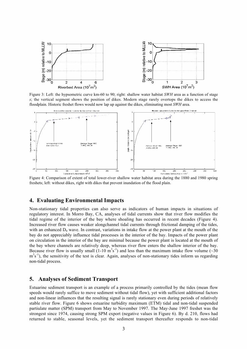
Figure 3: Left: the hypsometric curve km-60 to 90; right: shallow water habitat SWH area as a function of stages; the vertical segment shows the position of dikes. Modern stage rarely overtops the dikes to access thefloodplain. Historic freshet flows would now lap up against the dikes, eliminating most SWH area.

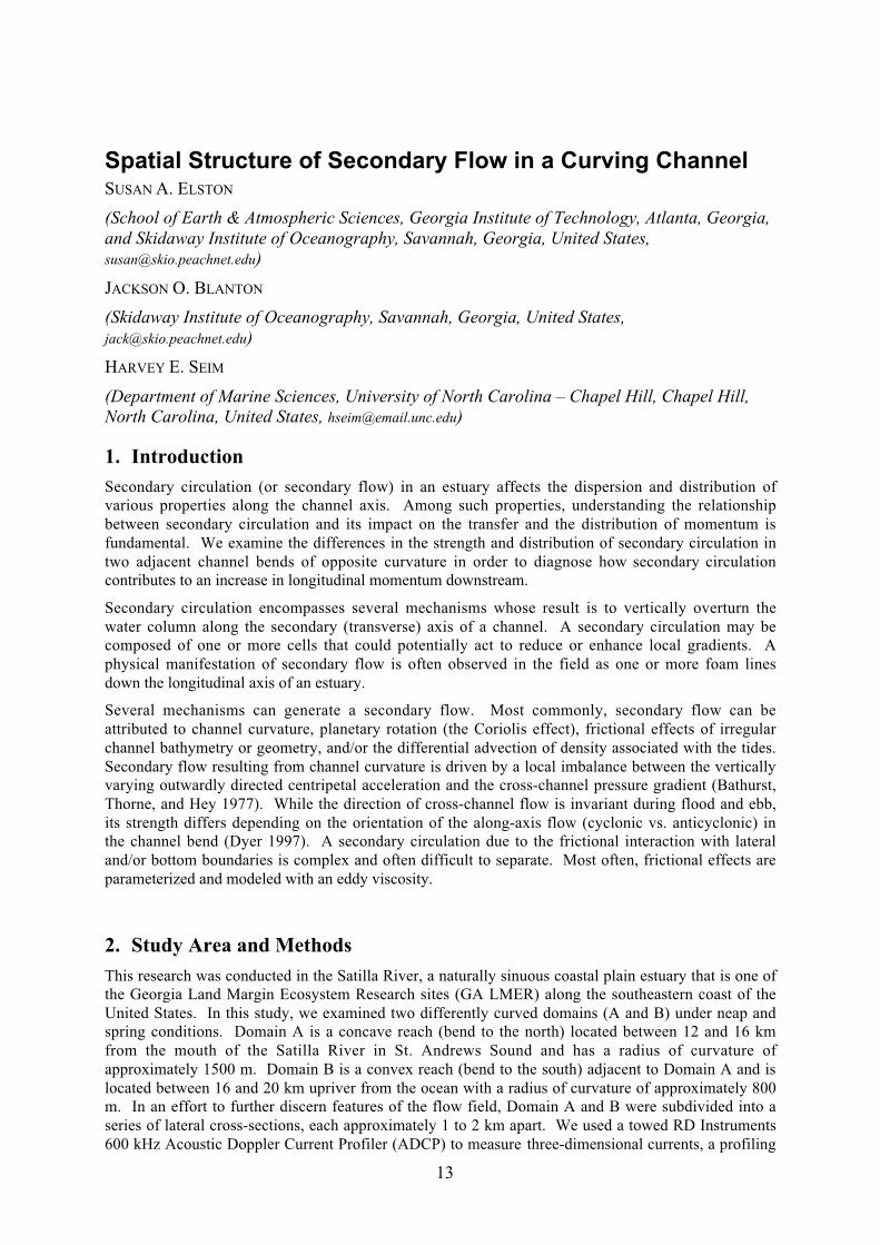
Figure 4: Comparison of extent of total lower-river shallow water habitat area during the 1880 and 1980 springfreshets; left: without dikes, right with dikes that prevent inundation of the flood plain.

4. Evaluating Environmental ImpactsNon-stationary tidal properties can also serve as indicators of human impacts in situations ofregulatory interest. In Morro Bay, CA, analyses of tidal currents show that river flow modifies thetidal regime of the interior of the bay where shoaling has occurred in recent decades (Figure 4).Increased river flow causes weaker alongchannel tidal currents through frictional damping of the tides,with an enhanced D4 wave. In contrast, variations in intake flow at the power plant at the mouth of thebay do not appreciably influence tidal processes in the interior of the bay. Impacts of the power planton circulation in the interior of the bay are minimal because the power plant is located at the mouth ofthe bay where channels are relatively deep, whereas river flow enters the shallow interior of the bay.Because river flow is usually small (1-10 m3s-1) and less than the maximum intake flow volume (~30m3s-1), the sensitivity of the test is clear. Again, analyses of non-stationary tides inform us regardingnon-tidal process.

5. Analyses of Sediment TransportEstuarine sediment transport is an example of a process primarily controlled by the tides (mean flowspeeds would rarely suffice to move sediment without tidal flow), yet with sufficient additional factorsand non-linear influences that the resulting signal is rarely stationary even during periods of relativelystable river flow. Figure 6 shows estuarine turbidity maximum (ETM) tidal and non-tidal suspendedpartiulate matter (SPM) transport from May to November 1997. The May-June 1997 freshet was thestrongest since 1974, causing strong SPM export (negative values in Figure 6). By d. 210, flows hadreturned to stable, seasonal levels, yet the sediment transport thereafter responds to non-tidal

4

influences (e.g., wind waves re-suspension in peripheral areas) such that the resulting mean and tidaltransports are episodic. They could not be predicted or accurately described using conventional tidalanalysis tools.

Figure 5: D4 alongchannel current impedance amplitude vs. (left) the square root of river flow to tidal prism ratioand (right) the square root of power plant intake flow to tidal prism ratio. Anomalous high values at rightcorrespond to high-flow periods.

Figure 6: Subtidal (left) and tidal (right) SPM transport in the Columbia ETM at surface ( � ) and bed ( � )

6. Perspective on the Uses of Non-Stationary TidesConsideration of these examples of non-stationary tidal processes suggests two lessons. The first isthat the non-stationary part of tidal signals contains valuable information regarding the tidal responseto non-tidal influences and the non-tidal processes as well. The second point is that the assumption ofstationarity is actually a handicap when the signal is manifestly non-stationary. It was, for example,possible to achieve a compact and accurate method to predict river tides because the assumption ofstationarity was abandoned, and the apparatus of tidal constituents with it. When one recognizes asignal as non-stationary on times scales of days to weeks, then tidal constituents become useless. Tidalconstituents are useful as a means to represent the variability of tidal species only when tides arestationary over a long enough period (15 –30 d) to allow separation of the major constituents withinthe diurnal (D1) and D2 species. The species themselves are more robust. They remain useful up to thepoint where the modulation of tidal processes by external forcing is so rapid that D1 and D2 can nolonger be separated. This occurs when the spectrum of the non-tidal forcing extends from the subtidalup into the tidal band. Prediction of stationary tides is much the most successful form of geophysicalprediction ever devised. Precisely because tidal prediction has been so successful it is useful, possible,and necessary to move on to non-stationary tidal processes for new insights.

Acknowledgments: Development of wavelet tidal analysis tools and sediment transport analyses were supportedby the National Science Foundation. Applications were supported by the National Marine Fisheries Service, theUS Army Engineers, and Duke Energy North America.

��

��

��

� ��

�� !!"#�$�� %�� !&'#�

�� ( �� !&!# ��

�� !&&# � �� ) �� *"" #� +��

+�� ' �� ,-./�� 0� �� 1� �� $�� %�� 2��

� � � � ��

1� �� $�� 3�� 0� �� (�� 4� �� ( �� " ( �� ( �� 4$�13 �� 5 �� 5�6 �� 6 �� " ��

� �� "�* �� ( �� , �� ' ��

�� & � �� *"" (+7 ,-./ �� 8��(�� 9��* " �� " �� :�� ; �� "�6 �� :�� ,-./ ��;� �� ,-./ �� *6�� 5 �� .�� " �� $��

6

�� * �� < �� 5 ( � ��

��< �� :�= �� ; �� *�6�� < �� :��; ��

�� = �� >�

��

�� :��> ��; ��# : ;

�� < ��

� ��

�� ' �� :?�� ;� , �� ( �� :�� ''� !* �� "@;� 4� �� :�� @A �� * ;� �� "�5 ��

, ��( �� 6�� :�� '@ �� '&;� � � �� :*6 � �� A �� ;� �� 4� ��

B� �� *5 �� :�� !5;� - �� "�5 �� (�� (�� A" ��

�� *5 �� 1��

/�� :�� "5 �� "; � �� :�� "�5 ��; �� ,� �� %��

@

60 70 80 90 100 110 120 130−1

0

1

m s−

1

60 70 80 90 100 110 120 130

−0.1

0

0.1

m s−

1

60 70 80 90 100 110 120 1300

5

10

kg m−

3

60 70 80 90 100 110 120 1300

5

10

m s−

1

60 70 80 90 100 110 120 130−0.2

0

0.2

m

yeardays 2001

d

c

b

a

?�� C �� :;� �� :�� ;�� :�� ; �� :�;� �� '*�� %�� :�; �� '*�� :�� ; �� %�� :�� ;:�;� 1�� /��

� ��

�� :�� "5 �� ;� �� %�� %�� 1�� !&&#�� B � �� 1� �� $�� (�� :�� "�A ��; � �� +�� 2��

'

��

��

�� ! ��"

��

D�� -� ��E $� .� 8�� E /� +�� -� $� /�� $�� .��(� 8�� **A*�**5"� !&'�

�� /�� )� 3� 1�� D�� 5& �5!'� !&@�

4 �� F7� G� ,�� D� $� �� )� G� �� 1�� 1�� ! "�� #� A@ �A''� !&!�

1�� )� �� )� +� 1�� 1�� 8� �� "�� $� *!6�A A� !!6�

1�� )� +�E )� 8��E )� �� D� ,�� %� *6� A*� !!"�

1�� E )� 8 � �� 1� D� �� .�� &'� '" A� '"A'� *"" �

&

9

The role of the tide on the salt wedge displacement andmixing in the Itajaí estuary, southern BrazilCARLOS A.F. SCHETTINI

(Center of Earth and Marine Sciences, University of Vale do Itajaí, C.P.360, 88302.202,Itajaí, SC, Brazil, [email protected])

KLAUS RICKLEFS

(Research and Technology Centre Westcoast, University of Kiel, Hafentoern, 25761, Buesum,Germany, [email protected])

RODRIGO ZALESKI

(Center of Earth and Marine Sciences, University of Vale do Itajaí, C.P.360, 88302.202,Itajaí, SC, Brazil, [email protected])

STEFAN BRANDT

(Research and Technology Centre Westcoast, University of Kiel, Hafentoern, 25761, Buesum,Germany)

1. IntroductionThe Itajaí estuary is a microtidal salt-wedge type, river dominated where the main transportmechanism is the fluvial advection. The regime of the fluvial discharge is irregular along the time,with random distribution of flood peaks as response of the sub-tropical weather instabilities. Ongeneral basis, the estuarine hydrodynamics can be distinguished in two main modes. There is aintermediate to high discharge periods mode, which usually lasts for hours to few days and are highlydominated by the river freshet, and the low discharge mode observed between the flood peaks, whichcan lasts for several months (Schettini, 2002).

The river discharge is the main driven determinant of estuarine hydrodynamics in general terms. Thesalt intrusion follows an inverse and non-linear relationship with the river discharge. During prolongedlow discharge periods the salt intrusion can reach more than 30 km upstream. During mean dischargeperiods the salt intrusion is about 15-20 km upstream. When the discharge exceed 1000-1200 m3.s-1 allsalt water is flushed out of estuarine basin (Schettini & Truccolo, 1999). The position of salt intrusionis not a simple function of the river discharge, but also is a function of the time elapsed since the lastflash flood.

During periods of low river discharge the tide gain weight on hydrodynamics control. The role of thetide was previously assessed through some 25-hour experiments, given a site-specific interpretation.The objective of this paper is to assess the influence of the tide through the observation the salinitydistribution along the all estuary in high and low tidal phases and along a complete spring-neap cycle.

2. Field data & data reductionTo evaluate the role of the tide it was performed daily during 15 days surveys twice a day, at low andhigh tide. Salinity vertical profiles were acquired every 1-1.5 km from the mouth to upstream of thesalt intrusion using a real-time CTD probe ME-Grisard (www.me-grisard.de). Every survey wascarried out in less than 1.5 hour, giving us a quasi-synoptic view of estuarine structure at a given tidalphase.

Daily river discharge data were obtained with the National Electric Energy Agency (ANEEL) for theIndaial lymnimetric station, situated at 90 km upstream of estuarine mouth.

10

The raw data acquired with the CTD probe were reduced for 0.25-m vertical resolution using Matlabroutines (Mathworks, Inc.). The longitudinal salinity distributions were made using Surfer software(Golden Softwares, Inc.). The maximum salt intrusion of 2 and 30 ‰ isolines were extract then fromthese maps.

The mixing was evaluated by the total content of mixed water along the estuary. The mixed water wasdefined as the water with salt concentration between 2 and 30 ‰. Fresh and salt waters were thosewith salinity lesser than 2 and higher than 30 ‰, respectively. The proportion of water masses wasachieved by measuring the area distribution of each other on the salinity distribution maps. Thenarrowness of the estuary, as well as the no existence of intertidal areas justifies this procedure.

3. ResultsThe Figure 1 presents a synthesis of the results. During the 15-day experiment the tidal height betweenconsecutive surveys varied from 0.7 at the beginning and at the end of the period, to 0.2 at the middle,clearly indicating the spring-neap cycle (Figure 1A). The river discharge was low during the first 7days, with a flash flood discharge peak at 8th day, disturbing the experiments. Even thus, we continuethe experiment as we saw the opportunity to evaluate the estuarine response to the flash flood and thesalt intrusion after that (Figure 1B).

During the first eight days of experiment, before the flash flood, the salt intrusion ranged from 17 to21 km, considering the 2 ‰ isoline, and 4 to 12 km, considering the 30 ‰ isoline. Along this periodthe isolines of low and high water converges as the tidal height decrease, reaching the smallestdifference about of 2 km at January 14th. After the flash flood peak, the isolines were pusheddownstream up to 4 km from the inlet. The low water isolines stayed nearly stationary, mainly the 30‰, meanwhile the high water isolines just start move upstream after the flash flood cease and decreaseto about 500 m3.s-1 (Figure 1C).

The content of mixed water in the estuary varied according the variation of the tidal height and theriver discharge as well (Figure 1D). During the period before the flash flood, the content of mixedwater increased from high water to low water. A steady behavior was observed during the first five-day period, with about 50 % of mixed water at high water, and about 80 % at low water. During thesedays the tidal height were higher than 0.5 m. At the 6th day, the tidal height decreased bellow 0.4, andsince then the content of mixed water was practically the same for both high and low water, andslightly lesser than in previous days. After the flash flood peak the content of mixed water during thelow water became smaller than the high water, staying like this until the end of the experiment whenthey reverse again although staying close each other.

The relationship between tidal height of consecutive surveys and the displacement of the salt intrusionis presented in the Figure 2, regarding to both limits of 2 and 30 ‰. There is a significant differencebetween them, where the 30 ‰ reference appears to be more efficiently controlled by tide than the 2‰. The explanation coefficient for the former was r2 = 0,76, meanwhile for the latter it was r2 = 0,14.The curve slopes also demonstrate the higher tide dependence of the 30 ‰ horizontal displacementthan the 2 ‰.

The results support partially the hypothesis that tide do not play a role in the estuarine hydrodynamics.This is thru when the tidal height is less than 0.4 m, when the salt intrusion can be close of a saltwedge at a rest. On the other hand, when the tidal heigh is higher than 0.5 m, it appears that theestuary experiment periods of intense mixing during the ebb phase (e.g., Dyer, 1997), when thecontent of mixed water increase.

11

0

5

10

15

20

25

Days (January, 2000)

7 9 11 13 15 17 19 21

0

20

40

60

80

100

0.2

0.3

0.4

0.5

0.6

0.7

0

200

400

600

800

1000

high water

low water

2 ‰ low water

30 ‰ low water

2 ‰ high water

30 ‰ high water

A

B

C

D

Figure 1:(A) daily tidal heigh, (B) river discharge, (C) 2 and 30 ‰ haloclines horizontal position and (D) mixedwater content in the estuary along the fortnight monitored period.

12

δH (m)0.1 0.2 0.3 0.4 0.5 0.6 0.7 0.8

-2

0

2

4

6

8

789 10

11

12

13

15

16

17

18

19

21

20

78

9

10

11

12

13

16

17

18

19

21

20

Figure 2: Relationship between the tidal height and 2 (circles) and 30 ‰ (triangles) isolines horizontaldisplacement. The numbers mean the month days.

Acknowledgments: The results presented here are part of the joint cooperation project “transport andtransformation processes in the Itajaí estuary - Transit”, between University of Kiel and University of Vale doItajaí, funded by DLR/Germany and ProPPEx/Univali./Brazil.

References:

Dyer, K.R., Estuaries, a physical introduction, New York, John Wiley & Sons, 195p, 1997.

Schettini, C.A.F., Caracterização física do estuário do Rio Itajaí, Revista Brasileira de RecursosHídricos, 7, 123-142, 2002.

Schettini, C.A.F. & Truccolo, E.C. Dinâmica da intrusão salina no estuário do Rio Itajaí-açu. In:Congresso Latino Americano de Ciências do Mar, 8, Trujillo, Perú, Resumenes ampliados…Tomo II,UNT/ALICMAR, p639-640, 1999.

13

Spatial Structure of Secondary Flow in a Curving ChannelSUSAN A. ELSTON

(School of Earth & Atmospheric Sciences, Georgia Institute of Technology, Atlanta, Georgia,and Skidaway Institute of Oceanography, Savannah, Georgia, United States,[email protected])

JACKSON O. BLANTON

(Skidaway Institute of Oceanography, Savannah, Georgia, United States,[email protected])

HARVEY E. SEIM

(Department of Marine Sciences, University of North Carolina – Chapel Hill, Chapel Hill,North Carolina, United States, [email protected])

1. IntroductionSecondary circulation (or secondary flow) in an estuary affects the dispersion and distribution ofvarious properties along the channel axis. Among such properties, understanding the relationshipbetween secondary circulation and its impact on the transfer and the distribution of momentum isfundamental. We examine the differences in the strength and distribution of secondary circulation intwo adjacent channel bends of opposite curvature in order to diagnose how secondary circulationcontributes to an increase in longitudinal momentum downstream.

Secondary circulation encompasses several mechanisms whose result is to vertically overturn thewater column along the secondary (transverse) axis of a channel. A secondary circulation may becomposed of one or more cells that could potentially act to reduce or enhance local gradients. Aphysical manifestation of secondary flow is often observed in the field as one or more foam linesdown the longitudinal axis of an estuary.

Several mechanisms can generate a secondary flow. Most commonly, secondary flow can beattributed to channel curvature, planetary rotation (the Coriolis effect), frictional effects of irregularchannel bathymetry or geometry, and/or the differential advection of density associated with the tides.Secondary flow resulting from channel curvature is driven by a local imbalance between the verticallyvarying outwardly directed centripetal acceleration and the cross-channel pressure gradient (Bathurst,Thorne, and Hey 1977). While the direction of cross-channel flow is invariant during flood and ebb,its strength differs depending on the orientation of the along-axis flow (cyclonic vs. anticyclonic) inthe channel bend (Dyer 1997). A secondary circulation due to the frictional interaction with lateraland/or bottom boundaries is complex and often difficult to separate. Most often, frictional effects areparameterized and modeled with an eddy viscosity.

2. Study Area and MethodsThis research was conducted in the Satilla River, a naturally sinuous coastal plain estuary that is one ofthe Georgia Land Margin Ecosystem Research sites (GA LMER) along the southeastern coast of theUnited States. In this study, we examined two differently curved domains (A and B) under neap andspring conditions. Domain A is a concave reach (bend to the north) located between 12 and 16 kmfrom the mouth of the Satilla River in St. Andrews Sound and has a radius of curvature ofapproximately 1500 m. Domain B is a convex reach (bend to the south) adjacent to Domain A and islocated between 16 and 20 km upriver from the ocean with a radius of curvature of approximately 800m. In an effort to further discern features of the flow field, Domain A and B were subdivided into aseries of lateral cross-sections, each approximately 1 to 2 km apart. We used a towed RD Instruments600 kHz Acoustic Doppler Current Profiler (ADCP) to measure three-dimensional currents, a profiling

14

Falmouth Scientific Instrument Conductivity-Temperature-Depth (CTD) sensor, and a flow-thruThermosalinograph (TS) system to capture synoptic variations in temperature, salinity, andbathymetry.

In order to describe the how the longitudinal momentum is transported laterally by secondarycirculation, we systematically defined the along and cross-channel components of the flow field byrotating the towed ADCP data in each domain along the principal axis as defined by the mean cross-sectional depth averaged transport. The advantage to forming the principal axis in this manner is toproperly weight the flow field for changes in bathymetry. The rotated component velocities were thenmultiplied by a constant density to form the quantities of axial (ρu) and transverse momentum (ρu) perunit volume. The lateral flux of along channel momentum per unit volume was formed by the productof the constant density and the along channel and cross-channel velocities (ρuv). This quantity isreferred to as the flux of total momentum through a cross-section.

3. Results and DiscussionSecondary flow observed during this experiment varied between 25 cm s-1 and 75 cm s-1 on thefortnightly time scale. The highest transverse velocities were observed during spring tide in cross-sections where the ratio of the effective channel width to radius of curvature was near unity. Forsimplification, we consider four adjacent cross-sections (two in Domain A and two in Domain B)during maximum ebb at spring tide when the signal of secondary circulation in the Satilla ismaximized.

In each cross-section, we found a persistent transverse circulation pattern that was consistent withsecondary flow driven by channel curvature. In concave Domain A, near surface transverse velocitieswere directed toward the north while flow at depth was directed toward the south. Similarly, inconvex Domain B, near surface transverse velocities were directed toward the south while flow atdepth was directed toward the north.

Cores of maximum axial and transverse momentum were observed in each cross-section and increasedin strength downstream. The core of maximum axial momentum was most often located in or near theshallows while the core of maximum transverse momentum was found shifted to the side of the axialmomentum core, toward the outside of the channel bend. The observed cross-channel flux of totalmomentum is consistent with flow directed along the thalweg (i.e., the lateral flux of axial momentumis directed toward the deep channel) and when plotted as a vector diagram, this data resemble thetransverse velocity flow pattern.

Observations of axial and transverse velocities are used to determine the reasonableness of the spatialand temporal characteristics of the secondary flow in the cross-sections. In a similar manner, thespatial and temporal attributes of changes in the location of core momentum between cross-sectionsare used to determine if a change in its location is consistent with flow due to secondary circulation.The continuity equation is used to calculate the vertical velocity and to provide a time estimatefor the vertical transport of momentum by the transverse circulation. Assuming typical axialand transverse velocities for the Satilla River during this experiment (U =1 m s-1, V = 0.4 m s-1), we determine that the vertical velocity (W) is 0.6 cm s-1. Given this verticalvelocity, the time for a water parcel in the secondary circulation to reach the bottom of the watercolumn is 2500 s (~ 42 minutes), and it must travel an axial distance of 2.5 km to reach a positionsimilar to its starting point in the transverse circuit. These results suggest that a secondary circulationcan be best described as a three-dimensional helix in the axial direction, in contrast to a closedcirculation cell at one location in space.

Next, using the observed axial velocity, the measured distance between adjacent cross-sections, andthe measured lateral distance that the momentum core shifted at each cross-section, we calculated thelateral velocity. The calculated lateral velocities were consistent with the observed lateral velocities ineach cross-section, including those significantly different due to changes in channel width and radius

15

of curvature. Based on our observations, we found that the time for a water parcel located in the coreof momentum to reach the bottom of the water column was around 2100 s (35 minutes) and it traveleda distance of 2.2 km downstream before returning to a similar position in the transverse circulation.These results are consistent with the observed changes in the location of the core momentum betweenadjacent cross-sections. This suggests that secondary circulation is responsible for the observed lateralshifts in core momentum between the cross-sections in two opposing bends in a predictable, helicalpattern. We illustrate the nature of the helical flow pattern in Figure 1, which is based on a realizationof the observed momentum field at spring tide in Domain A during maximum ebb. Note that thelengths of the arrows in Figure 1 are different. They schematically represent the three-dimensionalhelical structure of the secondary circulation and demonstrate that there is an imbalance in the lateralflux of along channel momentum in the downstream direction (i.e., momentum increases downstreambecause of secondary flow).

Figure 1: Schematic of momentum transfer in a lateral cross-section of the Satilla River by secondary circulation.The contours are of transverse velocity in m s-1. The different length arrows are used to represent the three-dimensional helical nature of the secondary circulation and show that there is an imbalance in the lateral flux ofalong channel momentum in the downstream direction.

These results are consistent with our previous studies, which show that the primary mechanism fordriving secondary flow in the Satilla is channel curvature. The observed secondary circulation patternwas as expected and as predicted by theory, in which transverse flow is to the outside of the channelbend at the surface and toward the inside of the channel bend at depth. Observed secondary flow inthis estuary is considerably higher than simple scaling arguments would suggest and often varies onaverage between 30 cm s-1 and 50 cm s-1 on the fortnightly time scale. Observed secondary flow alsovaries within and between cross-sections due to varying effective channel width and local radius ofcurvature.

Our calculations for the transit time and the distance to complete a secondary circulation are smallerthan but on the same order as those of Seim et al. (in press). They estimate that a water parcel startingnear the centerline of the channel will take approximately 100 minutes to complete a circulation andwill travel approximately 3 km downstream before it returns to its starting location in the transversecirculation. The differences between our results and those of Seim et al. (in press) are due primarily todifferences in the timing, location, and nature of the two experiments. Observations by Seim et al. (inpress) were based on a moored ADCP that sampled the flow field once every 15 minutes. Theirobservations were made in the deep channel for a 10-day period that ended shortly before themaximum spring tide. The design of their experiment focused on processes in the along channeldirection and consequently did not capture any lateral information. The disparity in the observed axialvelocities and resultant calculations between these two studies is due directly to the availability of thislateral data. Despite these differences, our results support the conclusions of Seim et al. (in press) that

16

the shape of the secondary circulation is helical and that when secondary flow is super-imposed on theaxial flow field it leads to an increase in the flux of momentum in the downstream direction.

4. Conclusions and ImplicationsOur research supports previous studies and extends the understanding and description of the lateralvariability in the ‘spatial structure’ of secondary flow. We demonstrate that secondary flow(secondary circulation) is best described as a helix down the axis of the estuary and that it has a non-negligible contribution to the momentum flux in the downstream direction. The implication is that thestrength and presence of a secondary circulation significantly modifies the momentum balance andcannot be neglected. Knowledge of the role secondary circulation plays in changing the distribution ofmomentum will better enable us to predict important parameters such as the length of the salt intrusionand to determine the dispersion and distribution of various waterborne properties (e.g., larvae,sediment, and pollutants) in the estuarine environment.

Acknowledgements: The authors acknowledge the financial support of the Land Margin Ecosystem ResearchProgram of the National Science Foundation (Grant No. DEB 9412089) to the University of Georgia and theState of Georgia through its Coastal Zone Management Program, and a Presidential Fellowship to the leadauthor from the Georgia Institute of Technology.

References:

Bathurst, J. C., C. R. Thorne, and R. D. Hey, Direct measurements of secondary currents in riverbends, Nature, 269, 504-506, 1977.

Dyer, K. R., Estuaries: A Physical Introduction, Second Edition. Chichester, England: John Wiley &Sons, Ltd, 1997.

Seim, H. E., J. O. Blanton, and T. F. Gross, Direct stress measurements in a shallow, sinuous estuary,Continental Shelf Research, in press.

��

��

��

��

��

� ��

�� Æ�� Æ�� !�� " � � � �� #�$�� %�� &�� !�!�� " � #�� !�� #�� #!��' �� #�! ��( � � �� " ��)� *#� �� !!��'�#�� #�'�#�# +�� +��,�� '�� ,�� '�� " �� *#� ��!��&��( � � ��,�� #�� !��!�� &�� )� ##� �� --. �" � � �#�� "�� +�� /�� 0��( 1&�� &�� #� ��(

2�!�� ,��#�� &�� !�!�� 3�4��5� ��

3�4445 �� 3��5�� &� �� !�� ! � �" � � ��( � ��!�!�� +�� " !�� !�� #�� #�� #�� " � � �� ( 6�&�� * �" �� 7�� #!�� &� �&��&��+ �" � � ��! �� " � � �� +�� %�� !�� 8� ��(

9� � � �� " �44� � � �� 6�&��#�� ,�� +�� 7�� !��$�� #�� #�� :�� #!�� &��8�� #!�� !�� "�� #�� ##�� +�� +�� ; �� !��"��#�� !�� ! �� &�� " !��!�� +�� #� �� #!�� !�� ! �� #�� ( � �&�� 8�� +� #�� +�� < 1�� =>/,) �� =>/,� �� #�� 9��?�� - �� #�� =29 12>@ !��8�� " �� *A%( � � !��8�� &�� &�� +� �#!�� +�� B,�< �� ,�� !�� (- �#� �� #� �" � � 9��?�� - �� #��(:�� ! �� +�� !��!�� +�� #!�� +�� - �� B,�4 >�2(

� � #�� " � � �� !�� " � ��#!�� &� �� "� � �� + �� +�� ! � �� #�� &�� "�� +�� $�� (

� � ��

��

2�� ##�� #�'�#�# ��C�� #�� #!�� ! �� Æ> ��+�� +��#�� "�� +�� D �4(4Æ>� �� &�� "��

+�� 4,��( 9� � � +�� #�� &�� C�� #��#!�� " � � �� " �(�,�(-Æ>� �� C�� " #�� Æ> �� &�� ( B'��!� "�� @��E�� > �� -�� !�� ! �� #�� &�� #�� +�� +�� &�� <(-( 1� � � ��" �� &�� +�� &� �)( �� #�� &�,�&�� #!�� + �� &�!�� +�� !��!�� !�� #� �� " � � ��(

�� !��!�� +�� +�� 7�� "��# � �� ##�� + �� !��!��( A��%�� #�� C�� "�� +�� ! �� -(� ��+�� #�� $�� ( � �&�� C�� #�� #�� !�� +�� C�� "#�� &�� ( >�#!�� ##�� #!�� +�� #�� #�� (

:�� F /�! �"�� ,�� +�� ,�� " � � ��#�� #�� 12>@� � � #��,�� "��##�� ( � �#��#�� +��#� +�� !��,"��#�� #�� ,�� "�� +��,�� +� ��(

39oW 54’ 48’ 42’ 36’ 30’ 24’ 18’ 12’ 18’

12’

6’

13oS

54’

48’

42’

36’

30’

•S1/S20

•S2 •S3

•S4 •S5 •S6

•S7

⊗S8

⊗S9

•S10 •

S11

•S12

•S13

•S14

•S15

•S16

•S17

⊕S18

⊕S19

⊕

•W21

♦

♦

♦

ITAPARICA IS

.SALVADOR

PA

RA

GU

AC

U R

IVE

R

ARATUBAY

←

MADRE DEDEUS CHANNEL→

SA

LVA

DO

R C

HA

NN

EL

ITA

PAR

ICA

CH

AN

NEL

• − Current meters

♦ − Meteorological Stations

⊗ − ADCP

⊕ − tide gauges

��

�� ##�� #�'�#�# !�� " ��(� # �� "��+�� +�� !�� " �� %� �� #�� %� �� ( �� "�� +�� #�'�#�# !�� -F�� &� "��# �� Æ( /�� +�� !�� +� �(� #G� +�� #�� (� # ��( H� +�� 8�� !�� &�� +��

+ �� &�� +�� !�� +� �� - # �� +�� #�� (�� (� # ��( � � �� +�� &� "��# �<�Æ� �� +�� #�� +�� Æ �� Æ�(

��

� � �� #�,�� +�� #!�� "�� ). �� . �"� � �� #!�� +�� &�� ##��( � � �#!�� " � �� &�� +�� (<< # �� (<� # �� 8��! � � �� + �� (�< # �� ( 1�� +�� ##�� #� #�� #!�� +�� G��

�� "��# �(�� (�4 �� (� � �� ! �� "��# 4�Æ �� 4Æ ��

�� #!�� #� �� " -� #�� +�� #�� ( 9� �� #�� ,�� #� �� +�� &��+�� -� #�� (� �� +�� ##�� !�� + �� ##�� +�� #�� !��(

� � ��#�� '!�� +�� 4�. �� 44. �" � � ��&�� &�� +� #�� !�� #�� " $�� (�4 # +�� (� �� #�� +�� ! �� +�� ! �� Æ ��" ! �� ##��(

��

� � �� ,� �� ,�� &��( � �� Æ�� !�� " &�� '!�� +�� !�� &�� #� �� + &�� &� �(4� �� . ��!��&��( ?�� Æ�� &�� " &�� '!�� +�� "��# � � �� #�� #!�� -(

� � #�'�#�# &�� +� �� " � � �� &�� > �� 9��!�� > �� )�� + �� #!�� #��" <� �# �� # �� !��&��( � � �� #!�� " �" � � ��

�� ( ?� �� " ��&�� #�� I�+ �� !�� " � � �� +�� # �� "�� /�� 2�� > �� + �� "�� I�+ "�� -� �# ��( 9� � � ��#�� #!�� "� � I�+ �� "��# �< �� # ��( ?�� #!�� 4 �� ( 9� � � �� #!�� ,�� #!�� &�� " #�� <� �# ��(

�� !� �� #�� " � � �� ,�� #��( :�� + �� +�� #� +�� #!�� +� ��!� � ��+� �� &�� " � � ��!� �� &�� #�� "�+ �� +�� #�(

��

� � �� +� �� "�� #� ��( 9��

� � �� "��# �##�� +�� &�� #�� +�� &�� '�� #�� 7�� <� *# �" ��&�� (

1� � � �� !�� " � � �� "�� I�+ �� + �� # �� I�+ �� +��( >�� #� !�� &�� " � � �� " � �# �� !��#�� "�� #�� &�� ( 1� � � ��+��+�� !�� " � � �� ) �� ) �� !��"�� +�� I�+ � �� !�� " � � ��I�+ �" � � �� 9��!�� > ��(

1!�� "��# �� , ��" �� ,�� ( 2�� ##�� !��#�� !!�� &�� ,+��+�� " �! �� # �� "�� 8,�� &�� +�� #�( 2�� +�� !��#�� +�� "��#�� I�+ �� +�� #�� #!�� ##��(

� ��

1�� ! �� 8�� +� ��","�� # �" +�� !��!�� ( 9�� !��#�� &�� !�� '!�� C�� "��#�##�� +��( ?�� I�� " �� #�� " ��#�� !�� &�� +�� #�� !�� #!��( 9" +�� #� �� +�� !��!�� + �� + �� " �� +�� +�� #!�� +�� (

�� !��

"#$%&'(##)* �� +,&+++(',)* -� �� .�� /�0�� 1�� 2��

!�0�� 0��

��

� � � � ��

J�� 6( >� 0( /( J( 2�#�� 1( >( ( @( �� 1( �� >�� " �� H�� %��F � �� %�,�� -�,�<�� (

/�� 1( /(� >( 1( :�� B( 0( 2( >�#!�� 9#!��E�K�� #�� L�� M��&�� @�� !�� E�K�� !��K�� #�� ,�� 444(

��#�� N( /(� �( >( �� @ J /�� ?��! � �� !�� #�� !�� ""�#�� )�,�)�� 4��(

21

Sill dynamics and energy propagation in a jet-type fjordMARK INALL, FINLO COTTIER, COLIN GRIFFITHS

(Scottish Association for Marine Science, Dunstaffnage Marine Laboratory, Oban. PA344AD, Scotland. Email: [email protected])

TOM RIPPETH

(School of Ocean Science, University of Wales Bangor, Menai Bridge, Anglesey LL59 5EY,Wales.)

1. IntroductionFjords may be classified into two broad categories: wave-type and jet-type. The division is dependenton the properties of the barotropic tide as it passes over the sill and the degree of stratification in thefjord basin. If flow is greater than the speed of the mode 1 internal wave (internal Froude number, Fr1,greater than 1), a tidal jet forms on the lee side of the sill. Physical pathways whereby the barotropicenergy is transformed at the sill and propagated through the fjord have implications for the efficacy ofvertical mixing in such jet-type systems. Furthermore, climatic and strategic considerations havemotivated much research in recent years of stratified flow over sill and through straits (e.g. Farmer andArmi, 2001). The upper basin of Loch Etive on the west coast of Scotland is a fine example of a jet-type fjord (Figure 1).

2. ObservationsA basin-wide survey of Loch Etive wasundertaken in June 2001 in an attempt to followthe pathways by which the barotropic energydisperses into, and dissipates within the loch.Moorings were deployed along the axis of thebasin, and instrumented with acoustic dopplercurrent meters (ADCPs), and temperature andsalinity sensors. Bottom pressure recorders werelevelled-in either side of the sill. Simultaneoustidal cycle surveys were undertaken over the sillusing a vessel mounted ADCP and a hand-heldCTD, and along the axis of the basin using atowed undulating CTD. Standard CTD profileswhere made at the reference stations RE1 to RE7(Figure 2).

Bottom pressure recorders have revealed both africtional mean sea level set-up of 0.11 m in theupper basin, and marked asymmetry in thebarotropic forcing of the upper basin, bothpresumably a result of tidal constrictions seawardof the sill. A simple hydrodynamic tidal modelhas been used to investigate the frictional valuesnecessary reproduce the free surface elevationmeasurements. The asymmetry is reflected in thetidal flows over the sill, with a fast flood tide anda slower, prolonged ebb (Figure 4).

Figure 1 Location map of Loch Etive (upper panel),coastal outline of Loch Etive system with standardCTD stations RE4 and RE5 shown (lower panel).

22

Figure 2 Bathymetric cross-section along the axis of the upper basin of Loch Etive: CTD stations RE1 to RE7(circles), current meter and T/S moorings (triangles), and experimental yo-yo CTD mooring (HOMER)

3. Jet forcing at the SillA detailed ADCP survey across the sill has allowed us to examine some of the sill processes,particularly those occurring on the lee side as the jet separates from the bed creating high vorticity andstrong vertical recirculation at that point (Figure 3).

Figure 3 Cross-sill flow at maximum flood tide from the sill (left), towards RE5 (right) from the vessel mountedADCP. The horizontal scale for the figure is 1500m.

Throughout the spring/neap cycle the inflow always becomes supercritical (Fr1>1) at some pointduring the flood tide (Figure 4b). Flow separation occurs throughout the spring flood tide of June 19,and is identified as a ‘post-wave’ regime, where separation occurs in the lee of the sill (Baines, 1995).Flow over the sill is intense enough to promote aspiration from twice the sill depth, and at high valuesof the non-dimensional parameter NH/U, where N is the buoyancy frequency, H is sill height, and Uthe flow over the sill (Figure 4c), separation is due to upstream blocking of denser fluid below theaspiration depth (approximatelty 35m). However at lower values of NH/U flow against the adversepressure gradient below the internal lee wave crest may also contribute to flow separation.

23

Figure 4 Depth avarage cross-sill flow from the sill-moored ADCP (a), bold line indicates supercritical flow.Baroclinic mode 1 Froude number (b). Non-dimensional parameter NH/U, values greater than 4 not shown (c).

4. Basin ResponseDespite the periodically high Froude numbers,moored instruments along the axis of the lochbasin have revealed large oscillations of thepycnocline (10 m amplitude) below sill depth,and pulse-like depressions in the pyconclineabove the aspiration depth (Figure 5) .

CTD data reveal gently sloping isopycnals alongthe basin axis, and linear theory predicts adecrease in the phase speed of the M2 baroclinicmode 1 internal oscillation (C1) from 0.71ms-1 atRE5, to 0.31 ms-1 at RE1. However, it appearsfrom moored thermistor, and towed, undulatingCTD records that the oscillations do notrepresent a linear internal wave train, and thepulse-like depression propagates from RE5 toRE1 with a constant speed of 0.2ms-1. There is apropagation of baroclinic energy away from thesill into the basin interior and we can estimatethe energy transfer and investigate the generationand dissipation.mechanisms.

The development of the pulse can be seen in theundulating CTD records (Figure 6). As the flood tide weakens, and the flow becomes sub-critical, adepression of the 21.6 sigma-theta surface develops (Figure 6a to 6c). As the flow then ceases, thepulse propagates away from the sill at 0.2 ms-1 (Figure 6c).

06:00 12:00 18:00 00:00 06:00 12:00-140

-120

-100

-80

-60

-40

-20

0

9.75

9.5

9.75

10.5

Figure 5 Temperature contours at RE5. No data areavailable below 100 m and above 20 m)

24

Figure 6 Contours of σθ from the towed undulating CTD on June 19. The center time for each section is shown,the horizontal scale for each panel is 3800m, running from RE5 to RE3 (from left to right in each panel).

5. EnergeticsFrom this detailed observational study of the forcing and response of a jet-type fjordic system, weshall go on to quantify the pathways of tidal energy, from the loss of barotropic tidal energy to theforcing and energy loss of a tidal jet, through to the transfer to the baroclinic field and ultimately tomixing. An attempt to do this in a wave-type fjord was partially thwarted by the sparsity ofobservations and complexity of the chosen fjord (Inall and Rippeth, 2002), however we anticipateproducing a more tightly constrained energy budget from this study.

References:

Baines, P.G., Topographic Effects in Stratified Flows, Cambridge University Press, Cambridge, 1995.

Farmer, D.M and L. Armi, Stratified flow over topography models versus observations, Proceedingsof the Royal Society of London A, 457, 2827-2830, 2001

Inall, M.E. and T.P. Rippeth, Dissipation of Tidal Energy and Associated Mixing in a Wide Fjord,Environmental Fluid Mechanic, in press, 2002.

��

�� !�� "�!#$$% &��'�� (� ��

� ��

�� ! �� "�� ! ��

J H

longitudinal velocityho

t wal

l

CONVECTIVE REGIMETRANSITION REGIME

longitudinal velocity

hot w

all

CONDUCTIVE REGIME

longitudinal velocity

hot w

all

isotherms, side view

hot w

all


hot w

all


hot w

all

# �� $% &'�� ' �� (� �� ! �� ! �� )�� $**+ �

�� & �� ,�� $*+- � � '�� .�� &��'��#�� /�� # �� $! �� 0 �� ! �� '�� %

�� 1�2��

��$

�� 1�

��-

� 1�

�3

-4

�� ! � �� ! � �� ! �� 2 �� 5��

(� �� ! �� # �� $ � #�� '�� # �� ! ��

� � ��

�� '�� ,�� (�� ! �� '��

Æ � �� 6

(� �� ! �� / �� ' ��

� � �� 4

#�� $ �� 5�� ! �� %

7 1 �$

��

��

��

�� 8

7 1 �$

��

�� +

� �� 9�� ! � � �� ! � � �� )� �� 5�� !�� :� �� Æ �� ! �� ! 2 �� ! �� !��

� ��2Æ�

� � �;

<�� /�� 6! 4 �� ;! )�� $**+ ��%

Æ�� *

�� '�� '��! �� (� �� ! �� "�� (��$*;7 ! �� /�� * � �� %

�� 1� �� $7

-8

−2 0 2 4 6 8

0

0.1

0.2

0.3

0.4

0.5

Imberger (1974)

Cormack et al (1974)

Kumar and Ostrach (1977)

Bejan et al (1981)

Loka (1979)

Simpkins and Dudderar (1981)

Simpkins and Chen (1986)

log( Ra A )2

intr

usio

n th

ickn

ess

# �� -% (�� '�� Æ�� $� $7� ��'�� Æ�� 1 3�- � �� )�� $**+ �

� ��

�� '�� # �� - � �� ! �� %

� +7 � �� $�4* � $7�

� + � �� $3;7 ��

� 7�7$ � � � 7�-4�

0�� <��' �� $*+6 ! �� =�� ! �� ! �� Æ�� 1 3�-�� $7� � �� '�� /�� )�� 1 $7�! �� '�� 7�4! �� 0� � ��/��! ��

-+

� ��

)� �� ! � � �� ,�� -77$> ?��'�@� ��)�� -77- � A�� ' �� <�� 5��)�� -77$ �

�� )�B�� 0�! 0��,�� 0� �� (�� C�! D�� 9�� 5�� ! �� !-;3�-**! $*;$�)�� )! <�� 5�� ! ��

�� ! 67! $+! 6$74�6$$6! $**+�)�� )! &�� ! � ��

��! *4! $74�$-8! -77$�<��' =�D! ��E� �� C�,� &� ��! .�� <�� 5�� ! "�� - .�� ! �� !"! -37�-68! $*+6�,�� C�D�! &�� ,�� ! �� #�� ! 8;+�8*+!$*+-�,�� 0�F�! (�� E�.� �� ?�)�! ,�� $�� ! %�! *4*�*+-! -77$�(�� C�! .�� <�� 5�� "�� 3� D�� ! �� !"! -6+G-87! $*+6�?��'�@� E� �� )� )��! D�� 5�� 5� � �� &�'� �� (� � �)��

��! :� �� F�� ! F�� ! &�� ! -77-�?�� 0� �� &� A��! <�� :� ��! =�� F�� 0�� D�� #�0&H��++�$3- �� )�B�� $*;$ $*++�� '�! F�&�� ! =�� F�� 0�� D��! <�� :� �� A�� $*;7 $*+*�&� A��! �� '�! �� 0� ?��! .�� ! �� *�� % ��! A��! #�� $*;7�C�<� "��! �� C� (��! :�� ! ��

�� +�! 84�;8 $*;7�"�E� & ��' �� =� =��! <�� 5�� ! �� ! 633�648 $*;$�"�E� & ��' �� ?�&� <��! <�� 9�� ! �� !!!-$�3*! $*;8�

-;

29

Estimation of the Vertical Eddy Diffusivity: Observation inSwan River EstuaryAMIR ETEMAD-SHAHIDI

(Department of Civil Engineering, Iran University of Science & Technology, Tehran, Iran,P.O. Box 16675-163, [email protected])

1. IntroductionA clear understanding of the vertical mass transport is of importance in both geophysical andenvironmental studies of stratified natural water bodies. The rate of vertical transport is commonlyparameterized by using the concept of vertical eddy diffusivity, kρ, which relates the vertical transportof the mass to the gradient of density profile. The magnitude of kρ is not constant may vary by severalorders of magnitude depending on the turbulence properties and background stratification. Therefore,it is necessary to quantify kρ for different situations. The common method for estimationg kρ ismicrostructure measurements in the field. Since direct mesurement of kρ is not an easy task in thefield [Etemad-Shahidi and Imberger 2001], indirect methods have been developed and invoked in thefield studies. These indirect methods have been used both in the lakes and ocean [e.g. Wuest et. al1996, Toole et. al 1994]. However, the statistics of the obtained values of kρ have been rarelycalculated. The purpose of this study is to address this issue in the pycnocline of an estuary.

2. Method

2.1 Osborn method

for a steady and laterally homogenous shear flow, using energy partitioning arguments, Osborn [1980]estimated the vertical eddy diffusivity as:

222.0

NN

bkOS

ε== (1)

where, b is the buoyancy flux, ε is the rate of dissipation and N is the buoyancy frequency. The maindisadvantage of this method is the uncertainty in the magnitude of b. This method, however, is stillused commonly in field experiments.

2.2 Osborn- Cox method

The method of Osborn-Cox [1972] is based on the balance between the production of temperaturevariance and destruction of it by molecular diffusion. For a steady and laterally homogeneousturbulent flow, the vertical eddy diffusivity is estimated as:

233 NKCkOC = (2)

where,C T x T x3 32

32= ( '/ ) / ( / )∂ ∂ ∂ ∂ is the vertical Cox number, and K is the molecular diffusivity

of heat and T′ is the temperature fluctuation.

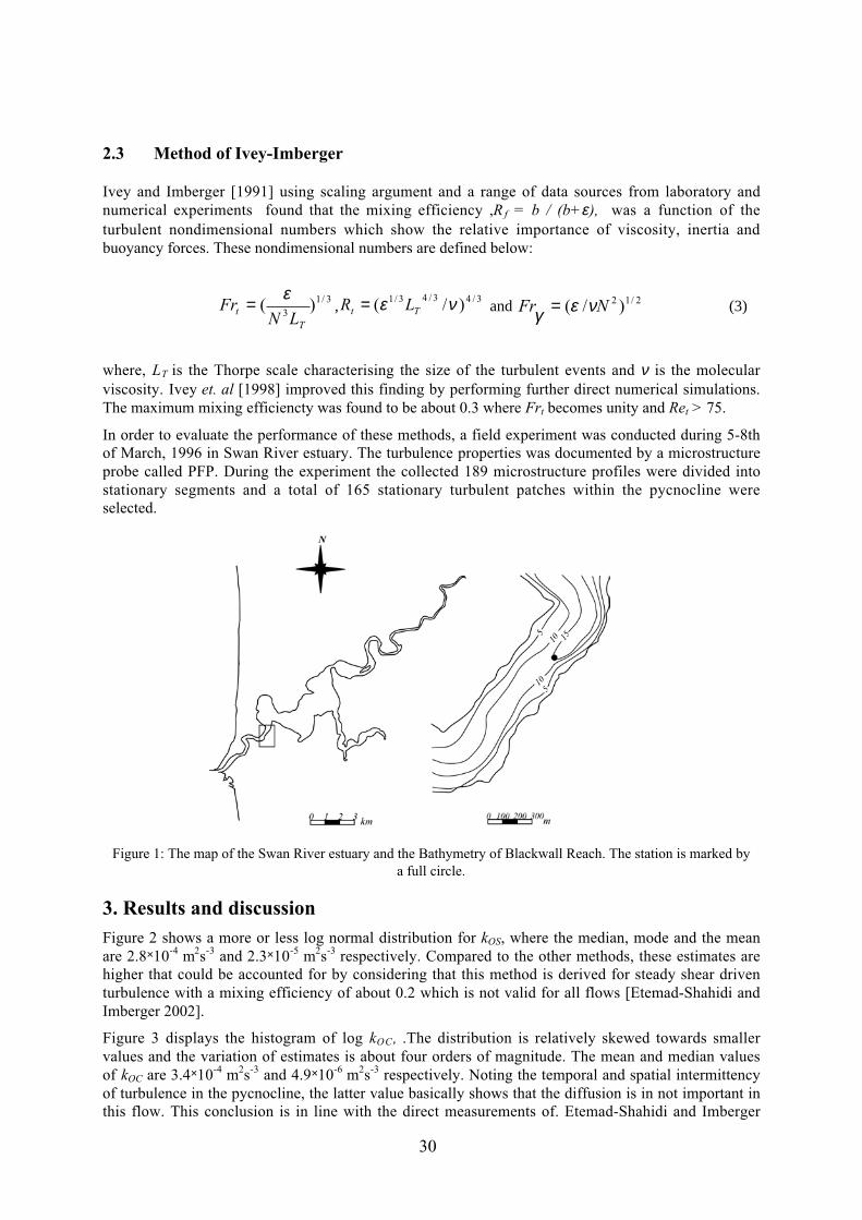
30

2.3 Method of Ivey-Imberger

Ivey and Imberger [1991] using scaling argument and a range of data sources from laboratory andnumerical experiments found that the mixing efficiency ,R f = b / (b+ε), was a function of theturbulent nondimensional numbers which show the relative importance of viscosity, inertia andbuoyancy forces. These nondimensional numbers are defined below:

3/13

)(T

t LNFr

ε= ,3/43/43/1 )/( νε Tt LR = and 2/12 )/( NFr νεγ = (3)

where, LT is the Thorpe scale characterising the size of the turbulent events and ν is the molecularviscosity. Ivey et. al [1998] improved this finding by performing further direct numerical simulations.The maximum mixing efficiencty was found to be about 0.3 where Frt becomes unity and Ret > 75.

In order to evaluate the performance of these methods, a field experiment was conducted during 5-8thof March, 1996 in Swan River estuary. The turbulence properties was documented by a microstructureprobe called PFP. During the experiment the collected 189 microstructure profiles were divided intostationary segments and a total of 165 stationary turbulent patches within the pycnocline wereselected.

Figure 1: The map of the Swan River estuary and the Bathymetry of Blackwall Reach. The station is marked bya full circle.

3. Results and discussionFigure 2 shows a more or less log normal distribution for kOS, where the median, mode and the meanare 2.8×10-4 m2s-3 and 2.3×10-5 m2s-3 respectively. Compared to the other methods, these estimates arehigher that could be accounted for by considering that this method is derived for steady shear driventurbulence with a mixing efficiency of about 0.2 which is not valid for all flows [Etemad-Shahidi andImberger 2002].

Figure 3 displays the histogram of log kOC, .The distribution is relatively skewed towards smallervalues and the variation of estimates is about four orders of magnitude. The mean and median valuesof kOC are 3.4×10-4 m2s-3 and 4.9×10-6 m2s-3 respectively. Noting the temporal and spatial intermittencyof turbulence in the pycnocline, the latter value basically shows that the diffusion is in not important inthis flow. This conclusion is in line with the direct measurements of. Etemad-Shahidi and Imberger

31

[2002] which showed that the down gradient flux in the turbulent patches is compensated with theconsequent up gradient flux within the turbulent events.

Finally figure 4 displays the histogram of log kII. The distribution is similar to the previous one. Themean and median values of kII are 9×10-5 m2s-3 and 6.6×10-6 m2s-3, respectively which are both close tothose of kOC. This could be explained by considering that both of these methods are obtained for steadyand laterally homogenous flows. In Brief it could be conferred that the method of Osborn is notappropriate for this flow and other indirect methods of Osborn-Cox or Ivey-Imberger gives a betterestimate of the rate of vertical eddy diffusivity.

Figure 2: Histogram of log kOS. The mean and median values of kOS are 2.8×10-4 m2s-3 and 2.3×10-5 m2s-3

respectively.

Figure 3: Histogram of log kOC. The mean and median values of kOC are 3.4×10-4 m2s-3 and 4.9×10-6 m2s-3

respectively. Note that a minimum value of 10-6 m2s-3 is assumed.

32

Figure 4: Histogram of log kII. The mean and median values of kII are 9.0×10-5 m2s-3 and 6.6×10-6 m2s-3

respectively. Note that a minimum value of 10-6 m2s-3 is assumed.

Acknowledgments: The author is grateful to Pecs2002 organizing committee for the awarded travel grant.

References:

Etemad-Shahidi A. and J. Imberger, Anatomy of turbulence in a narrow and strongly stratified estuary,J. of Geophysical Research-Oceans, under press, 2002.

Ivey, G. N. and J. Imberger, On the nature of turbulence in a stratified fluid. part 1 the energetics ofmixing, J. Physical Oceanography, 21:650-658, 1991.

Ivey, G. N., J. Imberger, and J. R. Koseff. Buoyancy fluxes in a stratified fluid, in Physical processesin lakes and oceans, Coastal and estuarine studies, 54, edited by J. Imberger, pp. 311-318. AGU, 1998.Osborn, T. R., Estimation of the local rate of the vertical diffusion from dissipation measurements, J.Physical. Oceanography, 10(1), pp. 83-89, 1980.

Osborn, T. R. and C.S. Cox, Oceanic fine structure. Goephysical Fluid Dynamics, 3 , pp.321-345,1972.

Toole, J.M., K. Polzin and R. Schmidt, Estimates of diapycnal mixing in the abyssal ocean, Science,264, pp. 1120-1123,1994

Wuest, A., D.C. Van Senden and J. Imberger, Comparison of diapycnal diffusivity measured by tracerand microstructute techniques, Dynamic of Atmosphere and Ocean 24, pp. 27-39, 1996

33

Trapped internal waves over undular topography andmixing in a partially mixed estuaryJULIE PIETRZAK

(Fluid Mechanics Section, CiTG, Delft University of Technology, Stevinweg 1, 2628 CN Delft,The Netherlands, [email protected])

ROBERT JAN LABEUR

(Fluid Mechanics Section, CiTG, Delft University of Technology, Stevinweg 1, 2628 CN Delft,The Netherlands, [email protected])

1. AbstractThe flow of a stratified fluid over small scale topographic features in an estuary may generatesignificant internal wave activity. Lee waves and upstream influence generated at isolated topographicfeatures, have received considerable attention during the last few decades. Field surveys of a partiallymixed estuary, the Rotterdam Waterway, in 1987 also showed a plethora of internal wave activitygenerated by isolated topography, banks and groynes. Additionally it revealed a spectacular series ofresonant internal waves trapped above low amplitude bed waves. The internal waves reachedamplitudes of 3 - 4 m in an estuary with a mean depth of 16 m. The waves were observed during thedecreasing flood tide and are thought to make a significant contribution to turbulence production andmixing. However, while stationary linear and finite amplitude theories can be used to explain thepresence of these waves it is important to further investigate the time dependent and non-linearbehaviour of these waves. With the development of advanced non-hydrostatic models it now becomespossible to further investigate these waves through numerical experimentation. This is the focus of thework presented here.

The non-hydrostatic finite element numerical model of Labeur was used in the experiments presentedhere. The model has been shown to work well in a number of stratified flow investigations. Here wefirst show that the model reproduces the field data and for idealised stationary flow scenarios that theresults are in agreement with the resonant response predicted by linear theory. Then we explore theeffects of non-linearity and time dependence and consider the importance of resonant internal wavesfor turbulence production in stratified coastal environments.

2. IntroductionUnderstanding the mechanisms for mass and momentum transfer in estuaries is a topic of widespreadinterest. Internal waves are known to play an important role in the transfer of mass and momentum.Observations in estuaries, laboratory studies and theoretical studies all suggest that internal waves mayplay an important role in the production of turbulent kinetic energy and mixing in estuaries. Internalwaves may be generated by various mechanisms, notably by sub-critical tidal flow over topography.Indeed since small scale topography is an ubiquitous feature of most estuaries and coastal seas, so tooare internal waves. The literature on stratified flow over topography is extensive, the study of thesubject began with the pioneering work of Long (1953) and more recently has been summarised in thereview by Baines (1995). Kranenburg and Pietrzak (1989) demonstrated through laboratory andanalytical studies that internal waves could increase the local production of turbulence by 40 % andsuggested that this could have significant effects for turbulence modelling in estuaries. Internal wavescan lead to mixing upon breaking. Pietrzak et. al. (1991) summarised the results from five fieldsurveys which were carried out in the Rotterdam. The surveys showed internal wave generation bysmall scale topography, freely propagating waves over a flat section of the estuary and internal wavegeneration and rotor formation by large scale features at the banks. Their study concluded that internal

34

waves contributed significantly to mixing and turbulence production in a partially mixed estuary. Herewe further investigate internal wave activity with the aid of a numerical model.

3. ObservationsThe Rotterdam Waterway is a man made tidal channel, with a predominantly semi-diurnal tide. Thefreshwater discharge at the head of the estuary is regulated so that the discharge tends to have aconstant value of about 2000 m3s-1. Dredging maintains the estuary at a constant depth, except for thebanks, so that generally only small scale topography persists. Two measuring boats were used in eachsurvey, one vessel was anchored and took profiles of velocity and density at 2 m depth intervals, whilethe other vessel recorded acoustic echo-sounding transects using a 210 khz transducer. The surveysrevealed the plethora of internal wave activity in the Rotterdam Waterway. The first two surveys dealtwith topographic wave generation over a pronounced series of bottom topographic features, withtypical bed wavelengths of 30-50 m and amplitudes of 0.5 - 1.0 m. It is the second survey that formsthe focus of the numerical simulations presented here.

Fig. 1 shows an example of resonant trapped internal waves over undular bed topography. Notably thewave height of the largest internal wave was approximately equal to half the water depth and theamplitude of the internal waves was 4-8 times the height of the topography.

Figure. 1 A 1 km echo-sounding showing internal wave activity along the axis of the Rotterdam waterway.Track 4 was taken between 15.46-15.52 h, 21 Oct. 1987. The tick marks are at 100 m intervals, Pietrzak et. al.(1990) and Kranenburg et. al. (1991).

During the ebbing tide a series of resonant trapped waves were observed. Initially the long wavecomponents in the topography were excited. The shorter wavelength components became apparent asthe tidal flow decelerated. For example, the wavelength seen in the images decreased from 80 m to 50m to 40 m to 30 m during Tracks 1 to 4, with amplitudes of 1 m, 2 m, 4 m and 4 m respectively.Finally Track 5 had a 3 m amplitude response with a wavelength of about 30 m. During the time of theobservations the Froude number decreased from 0.9 to 0.6. Tidal variations in the flow influence theinternal wave response. If the time variation is slow enough in comparison to the time scale of the tide,then quasi-steady theory can be used to interpret the data. In the previous analysis of the data Pietrzaket. al. (1990) and Kranenburg et. al. (1991) linear and finite amplitude analyses were carried out.These analyses help to identify the physical mechanisms causing the large amplitude response seen inthe acoustic images.

The conditions for resonance are satisfied if the free internal wavelength that coincides with theunforced internal wave equation has the same wavelength as the topographic forcing. If thetopography had been monochromatic only one wavelength would have been resonant and theamplitude of the response over the topography would be expected to diminish. However, since thetopography has contributions from other wavelengths it was possible for contributions from other

35

wavenumbers to become resonant as the tidal flow decelerated. In order to investigate this further anon-hydrostatic numerical model is employed.

4. ModelFINEL 3D, is the numerical model employed in these simulations. It has been developed by R.J.Labeur, while working at Svasek hydraulics, Royal Haskoning. It is based on the full Navier Stokesequations, with equations for temperature and salinity and an equation of state is used to calculatedensity. FINEL 3D is a fully 3-dimensional flow model. As no assumptions have been made withrespect to the vertical pressure distribution the model is suitable for non-hydrostatic flow simulations.The Navier-Stokes equations are discretised horizontally in space using a finite element grid, usingtriangular elements. An arbitrary number of vertical grid points can be used. The resulting coupled setof algebraic equations are solved with a fully implicit algorithm using BiCGSTAB as an iterativesolver. The transport equations for temperature and salinity are solved parallel to the flow equations.Subsequently, in each time step, the body forces resulting from the computed density distribution arecalculated and added to the equations of motion.

Fig. 2 Vertical velocities calculated from the analytical solution (above) and from the numerical model.

In this study the numerical model has been validated against linear small amplitude wave theory. Thebasic numerical set up consists of stationary flow over a series of sinusoidal bed waves. The horizontalextent of the model domain extends from –50 ≤ x ≤ 50 m. The vertical extent is 15 m. The bed waveshave a wavelength of 50 m and an amplitude of 0.25 m. This configuration compares with the flowsituation observed in the estuary. Fig. 2 shows the vertical velocities calculated from the analyticalsolution and from the numerical model. Good agreement is seen between the two. The phase errors arethought to be due to reflections from the open boundaries. A sponge layer was implemented at theopen boundaries in order to minimise boundary reflections, the simple sponge layer was found to bequite effective in reducing boundary reflections and minimising phase errors. A large amplitudeinternal wave response is also observed in the numerical experiments. The results from the numerical

36

simulations are in good agreement with those from linear wave theory, supporting the theory that thewaves are resonant trapped internal waves.

Further test cases are being carried out to explore the effects of internal waves on stratification in apartially mixed estuary. The estuary of particular interest to us is the Rotterdam Waterway, a partiallymixed estuary. Here data collected in 1987 have been reanalysed with the help of the non-hydrostaticfinite element numerical model FINEL3D. The model has been validated against linear wave theory.The model can reproduce the field data and for idealised stationary flow scenarios the results are inagreement with the resonant response predicted by linear theory. The non-linear model is an importanttool for scenario testing and furthering our understanding the effects of non-linearity and timedependence. Neither effect could be studied in detail with the simple analytical models employed sofar.

References:

Baines, P.G. Topographic effects in stratified flows. Cambridge University Press, pp 482, 1995.

Kranenburg, C. and Pietrzak, J.D. Internal lee waves in turbulent two-layer flow. J.Hydr. Engrg,ASCE, Vol.115 No. 10, 1352-1370, 1989.

Kranenburg, C., Pietrzak, J.D. and Abraham,G. Internal waves over undular bottom topography. J.Fluid Mech. 226, 205-217, 1991.

Long, R. R. Some aspects of the flow of stratified fluids. I. A theoretical investigation. Tellus, 5, 42,1953.

Pietrzak, J.D., Kranenburg,C. and Abraham,G. Resonant internal waves in fluid flow. Nature, 344,844, 1990.

Pietrzak, J.D., Kranenburg, C., Abraham, G., Kranenburg, B. and van der Wekken, A. Internal waveactivity in the Rotterdam Waterway. J.Hydr. Engrg, ASCE, Vol.117 No. 6, 738-757, 1991.

37

Quantifying turbulent mixing in a Mediterranean-type,microtidal estuary.JONATHAN SHARPLES

(Southampton Oceanography Centre, Southampton University, School of Ocean and EarthScience, Empress Dock, Southampton, SO14 3ZH, UK, [email protected])

MICHAEL COATES

(School of Ecology and Environment, Deakin University, PO Box 423, Warrnambool,Victoria, 3280, Australia, [email protected])

JOHN SHERWOOD

(School of Ecology and Environment, Deakin University, PO Box 423, Warrnambool,Victoria, 3280, Australia, [email protected])

1. IntroductionThe highly-stratified salt-wedge estuaries of southern Australia combine very small tidal influenceswith a Mediterranean climate in which river flows have a strong seasonal cycle. As a result ofnegligible freshwater inputs in summer and autumn, a sandbar usually builds up across the mouth,isolating the estuary from the open ocean. As rainfall increases in late autumn and winter, water levelsin the estuary gradually build up, until the mouth is forced open. River input can then flush the entireestuary with freshwater. Periods of lower river input result in upstream propagation of a salt wedge.River flow stops in early summer, and so the coastal alongshore transport of sand builds up at themouth to again block the estuary. During the blocked phase high salinity water becomes isolated in thebottom of deep basins along the estuary, with the strong halocline leading to the development ofanoxia and high sulphide concentrations.

The chemical, biological, and ecological environments are closely coupled to the timing of blockingand opening events, and thus to the patterns of seasonal rainfall. Throughout the year, but particularlyduring the blocked phase, the estuarine environment is controlled strongly by weak vertical mixingacross what is often a very strong halocline. As a first attempt to quantify the seasonal characteristicsof one of these estuaries, two experiments were carried out on the Hopkins River Estuary, Victoria,Australia, in April and in October 2000. The main objective was to observe the vertical turbulentmixing during the low current blocked phase (April), and during the high surface flow open phase(October). At the same time samples were also collected for nutrient and dissolved oxygen analysis,with the aim and quantifying the significance of the deep anoxic basins in the estuary for theproductivity of the surface waters that has been observed. The results illustrate the remarkably sharppartitioning between the surface and bottom waters, with very weak turbulent transfer between them.Nevertheless, despite the observed weak mixing, the presence of sharp nutriclines and oxyclinessuggested that the transfer rates of nutrients (ammonia and dissolved reactive phosphorus) from thebottom water into the surface layer, and of dissolved oxygen from the surface to the bottom waterwere quite high and capable of supporting significant surface productivity. This sharp transition inenvironments between the layers was associated with sharply defined regions of primaryphytoplankton and bacterial production. A thin, concentrated particulate layer, possibly of bacteria,just below the halocline during the blocked phase appeared to have a marked effect on the verticaltemperature structure of the estuary, apparently generating a localised region of convectiveoverturning.

38

2. MethodAt the start of each experiment an along-estuary survey of salinity, temperature, and dissolved oxygenwas conducted, using a YSI 600XL multi-parameter probe. Following the initial along-estuarysurveys, a number of fixed stations were sampled for turbulence and current characteristics, andnutrient and oxygen profiles. Vertical profiles of salinity, temperature, and turbulent dissipation (ε, m2

s-3) were measured using a Self Contained Autonomous Microstructure Probe (Ivey & Imberger,1990). SCAMP free-falls through the water at a nominal speed of 10 cm s-1, sampling at a rate of 100Hz. Salinity and temperature profiles were constructed with a 1 cm resolution from an accurateconductivity-temperature sensor. Turbulent dissipation was calculated by fitting the temperaturegradient wavenumber spectrum, as sampled by a differentiation circuit connected to each of two FP07thermistors, to the Batchelor spectrum (Ruddick et al., 2000). Vertical profiles of the verticaldiffusivity of density (Kρ (m s-2)) was estimated as a function of turbulent dissipation rate and the localbuoyancy frequency (e.g. Osborn, 1980).

Currents were measured with a 1200 kHz RD Instruments ADCP, with a 25 cm vertical bin size andan averaging period of 30 seconds (current s.d.=1.1 cm s-1). Water samples were collected using aonboard peristaltic pump connected to a nylon pipe and a close-interval sampling intake (Jorgensen etal., 1979). Samples for nutrient (ammonia, DRP, nitrate), dissolved oxygen, and sulphides werecollected with a vertical resolution of 50 cm (April) and 20 cm (October).

3. ResultsThe along-estuary survey of salinity in April 2000 showed the blocked phase of the estuary having atypical surface layer salinity of 10 to 12 ppt, with isolated deep pools in the upper estuary containinghigh salinity (25 � 30 ppt) bottom water (Fig. 1a). In contrast in October,

Figure 1. (a) Salinity section along the estuary, April 2000; (b) salinity survey, October 2000. The distances aremeasured from the Hopkins Bridge, about 700 metres upstream from the estuary mouth. Data could not beobtained below the bridge due to the lack of boat access.

much of the upper estuary, including some of the deep water, had a salinity of < 1.0 ppt, and a narrowsurface layer of approximately 1 metre thickness throughout the middle and lower reaches. There was

39

clear evidence of a well-defined wedge of saline water intruding up estuary a distance of 6 km (Fig.1b). Surface water in April had very high dissolved oxygen concentrations, typically 8 mg L�1

corresponding to 120% saturation, presumably reflecting high near-surface primary production rates.High salinity water in the deep pools, left over from the previous seasonal intrusion of the salt wedge,contained no dissolved oxygen and had very high concentrations of sulphide, reaching concentrationsof 500 mg L�1. The survey in October appears to have taken place after a freshwater input event hadpreviously flushed much of the estuary. The first deep pool (8.1 km) contained water predominantly ofsalinity < 1 ppt, with only the bottom sample having a higher salinity (5 ppt). The second deep pool(6.7 km) contained a deep layer of high salinity water and zero dissolved oxygen. Water of the samesalinity at the nose of the salt wedge had a dissolved oxygen concentration of 1 � 2 mg L�1, implyingthat the deep water at 6.7 km was old seawater left over from the previous blocked period.

Current measurements in April 2000 rarely exceeded 5 cm s-1 at the surface, 1 � 3 cm s�1 in the interiorof the deep basins, though sometimes showing near-bed increases to 3 � 5 cm s�1 at the bottom of thebasins. In October, surface flows ranged from 10 � 20 cm s�1 out of the estuary, usually over a bottomlayer weakly flowing upstream (1 � 2 cm s�1).

Figure 2. Vertical profiles of salinity, temperature, dissolved oxygen, NH4-N, and vertical turbulent diffusivity in(a) April 2000 and (b) October 2000. Error bars on the diffusivity profiles represent 95% confidence intervals,estimated using a bootstrap technique.

Examples of vertical profiles in the deep basin at 6.7 km from the bridge (Fig. 2) illustrate markedlydifferent environments during the 2 surveys. In April 2000 (Fig. 2a) the water was strongly stratifiedin two layers, with a low salinity (8 � 10 ppt) surface layer separated from a higher salinity (25 � 30ppt) bottom layer by a very sharp halocline (thickness ≈30 cm). A localised increase in temperaturewas also evident just below the halocline, associated with a layer of photosynthetic, sulphur bacteria.Turbulent diffusion was very low at the halocline (10-6 m2 s�1), with higher values at the surface andbottom boundaries (10�5 m2 s�1 and 10�4 m2 s-1 respectively). Nutrients were very low in the surfacelayer, increasing linearly below the halocline to the bed. The peak in NH4-N just below the halocline isfor the filterable (i.e. dissolved) form of this nutrient. (A 0.45 µm filter was used.) Dissolved oxygen

40

decreased exponentially away from the surface, dropping to 0 mg L-1 almost 1 metre above thehalocline. In October 2000 (Fig. 2b) the new seawater had apparently made further progress upstreamsince the time of the salinity survey in Fig. 1b, with a 3 layer structure showing old seawater below adepth of 7 metres, an intermediate layer of relatively new seawater input by the salt wedge, and anarrow surface layer of salinity < 1 ppt. Mixing across both haloclines was very low (10�6 m2 s�1),increasing at the surface (5 × 10�4 m2 s�1) and bottom (5 × 10�5 m2 s�1) boundaries. The recently-supplied moderate salinity water in the middle layer was already almost devoid of dissolved oxygen,and significant NH4-N was only available in the bottom layer.

4. ConclusionsThe two survey periods have illustrated two possible states of this intermittently closed estuary. Whenthe estuary mouth is blocked the deep pools in the estuary become anoxic and highly sulphurous,supporting a dense and layered community of phytoplankton and bacteria associated with a verystrong halocline. The oxygen demand by processes at and below the halocline can be estimated fromthe dissolved oxygen gradient and turbulent diffusivity to be approximately 8 g m�2 day�1. A majorsource of nutrients to the water column appears to be in the estuary sediments, with the flux of NH4-Nup through the bottom layer estimated to be about 50 mmol m�2 day�1. However, the observed nutrientspike at about 7 metres depth in April is believed to be sustained by re-mineralization of the organicmatter falling from the surface zones by bacterial communities just below the pycnocline. The largegradient that results is estimated to produce a flux of bacterially-produced NH4-N up through thehalocline of about 120 mmol m�2 day�1. This value shows the potental of bacterially-mediatedremineralization to supply nutrients into the overlying surface waters. In October 2000 a salt wedgeappeared to be returning seawater into the bottom of the estuary following earlier flushing byfreshwater. However, by a distance of 7 km into the estuary much of the dissolved oxygen in thiswater had been removed. Assuming a mean inflow speed of 2 cm s�1, and a typical wedge thickness ofabout 3 metres, it is estimated that the oxygen demand by the sediments amounted to a removal rate of5 g m�2 day�1. Diffusive flux of oxygen from the surface layer into the salt wedge was estimated to beonly 1 g m�2 day�1, insufficient to maintain oxic conditions in this highly productive estuary.

Our results show that there are two quite different estuarine environments under the two flow regimes.In April, the estuary has become, effectively, a meromictic lake containing a highly productive layerjust below the pycnocline. That layer is believed to supply, though diffusion, all the nutrients requiredby the overlying surface waters. In October, however, that layer is absent and the nutrients aresupplied by a combination of sources, such as by diffusion from the sediments, from river runoff andfrom the incoming salt wedge.

Acknowledgments: This research was supported by an Australian Research Council Small Grant. The authorswish to thank Colin Magilton and Alan Mainwaring for their assistance during the field programme.

References:

Ivey, G. N., and J. Imberger, On the nature of turbulence in a stratified fluid. Part I: the energetics ofmixing. J. Phys. Oceanogr., 21, 650-658, 1990.

Jorgensen, B.B., J. G. Kuenen and Y. Cohen, Microbial transformations of sulphur compounds in astratified lake (Solar Lake, Sinai). Limnol. Oceanogr. 24, 799-822, 1979.

Osborn, T. R., Estimates of the local rate of vertical diffusion from dissipation measurements. J. Phys.Oceanogr., 10, 83-89, 1980.

Ruddick, B. R., A. Anis, and K. Thompson, Maximum likelihood spectral fitting: the Batchelorspectrum. J. Atmos. Ocean. Tech., 17, 1541-1555, 2000.

41

A finite difference method for non-hydrostatic free-surfaceflows that is more accurate than Boussinesqapproximations but equally efficient.G.S. STELLINGA,∗ ,1 AND M. ZIJLEMAA,B

aFluid Mechanics Section, Faculty of Civil Engineering and Geosciences, Delft University ofTechnology, Stevinweg 1, 2628 CN Delft, The NetherlandsbNational Institute for Coastal and Marine Management/RIKZ, P.O. Box 20907, 2500 EX TheHague, The Netherlands

AbstractA numerical technique is presented for the approximation of vertical gradient of the non-hydrostaticpressure arising in the Reynolds-averaged Navier-Stokes equations for simulating non-hydrostaticfree-surface flows. It is based on the Keller-box method that take into account the effect of non-hydrostatic pressure with a very small number of vertical grid points. As a result, the proposedtechnique is capable of simulating relatively short wave propagation, where both frequency dispersionand nonlinear effects play an important role, in an accurate and efficient manner. Numerical examplesare provided to illustrate this; accurate wave characteristics are already achieved with only two layers.

KEY WORDS: free-surface flow; non-hydrostatic pressure; Keller-box scheme; wave propagation

1. IntroductionThe design of efficient and accurate numerical algorithms is an essential prerequisite for thesimulation of wave propagation from deep water through the surf zone, particularly for coastalengineering-type applications. Boussinesq-type wave equations with improved dispersioncharacteristics formulated by, e.g., Madsen and Sørensen [1] and Nwogu [2] are well suited to modeldifferent wave phenomena, especially in shallow water regions, such as nonlinearity, dispersion andshoaling. Also, these models include implicitly refraction and diffraction. Since, the Boussinesq-typewave models are based on an efficient depth-integrated formulation, they also have become verypopular for real-life applications involving wave dynamics in coastal regions and harbours. However,a well-known drawback of the Boussinesq-type modelling is the assumption of an irrotational andinviscid flow. As a consequence, neither the interaction of waves with rotational currents nor theeffects of viscosity on the wave motion can be simulated.

An alternative route is a numerical solution for incompressible turbulent fluid flows involving gravitywaves based on the time-dependent three-dimensional Reynolds-averaged Navier-Stokes equations.This approach is not only suitable to model wave-dominated flows over the entire range of waterdepths but also for simulating wave disturbance in real fluid with rotation and shear. A number ofstudies have been reported in which the features of this approach in the context of wave dynamicshave been investigated.

In the papers of Casulli and Stelling [3], Casulli [4] and Stelling and Busnelli [5], a fractional stepmethod is proposed that describes the inclusion of non-hydrostatic pressure by solving a Poissonequation in the hydrostatic free-surface flow model of Casulli and Cheng [6]. This hydrostatic modelsolves the 3D shallow water equations in Cartesian co-ordinates whereby the vertical accelerations areneglected and the vertical velocity is obtained from the (local) continuity equation. Such a model issufficiently accurate for large-scale flow phenomena like tidal and wind-driven flows in coastal seas,

∗ Correspondence to: Guus Stelling. Tel.: +31 15 2785426; fax: +31 15 27848421 E-mail: [email protected]

42

lakes, estuaries and rivers, but prohibits a correct calculation of short surface waves. The underlyingmotivation for the proposed fractional step approach is that the existing shallow water solver need notto be adapted, since the correction to the hydrostatic pressure is done after the shallow water equationshave been solved. As a consequence, this reduced the effort of software maintenance to a minimum.Moreover, Mahadevan et al. [7] have shown that this technique also leads to a more stable andefficient non-hydrostatic calculations than in a case without splitting the pressure into hydrostatic andnon-hydrostatic parts. An example of the latter procedure can be found in Mayer et al. [8], where 2DEuler equations including total pressure is solved and the surface elevation is determined by means ofa kinematic boundary condition along the free surface.

The method of decomposing the pressure into hydrostatic and non-hydrostatic components has alsobeen employed by Stansby and Zhou [9] and Zhou and Stansby [10]. However, their method isformulated in the sigma co-ordinate system, except for the horizontal non-hydrostatic pressuregradient which is retained in Cartesian co-ordinates since, sigma transformation of the horizontalgradients may introduce large truncation errors near a steep bed resulting from the summation of largeterms of opposite sign [11]. These truncation errors can cause spurious flows. Like Casulli andStelling [3], a conjugate gradient method is employed for the solution of Poisson pressure equation. Inthe former paper, they also demonstrated the use of their model for simulating waves and currents overtrenches and hills. Another procedure of similar purport is discussed by Li and Fleming [12].However, they discretized the momentum equations with the MacCormack’s explicit scheme and thussuffering from the CFL stability restriction related to the gravity wave speed. Furthermore, the Poissonequation for the non-hydrostatic pressure is solved by means of a multigrid technique.

It is recognized that sufficiently large number of vertical grid points is required in a 3D free-surfaceNavier-Stokes computation for describing wave dispersion characteristics up to an acceptable level ofaccuracy. In practice, this number is about 10 to 20; see, for instance, [4], [10], [12] and [13].Combined with the solution of the elliptic equation for the non-hydrostatic pressure, this greatlyincreases the computational effort that may hamper three-dimensional applications with a sufficientlyfine grid.

In this paper, we present an accurate approximation of vertical gradient of the non-hydrostatic pressurebased on the Keller-box or Preissmann scheme; see, e.g., [14]. This scheme belongs to the class ofimplicit finite difference schemes which are of a higher order of accuracy compared to the explicitschemes involving the same number of grid points. The scheme is also referred to as the Hermitianspline method, see, e.g., [15]. In fact, it is a discrete analogue of the Boussinesq-type of wave models;the vertical dependency of the non-hydrostatic pressure can be considered to be resolved by a finiteseries of spline functions. The splines are described by the pressure itself and its vertical derivative. Inthis manner, the implicit scheme calculates the vertical gradients of the non-hydrostatic pressure atdifferent vertical grid points simultaneously. The results presented in this paper show that thisprocedure allows a very small number of layers (in the order of 1 to 3) for the accurate simulation ofrelatively short waves. Even in the case of one layer, i.e. the depth-averaged mode, it predicts thefrequency dispersion for fairly short waves in shallow water with an accuracy similar to that of theBoussinesq-type wave model of Peregrine [16].

References

1. Madsen PA, Sørensen OR. A new form of the Boussinesq equations with improved lineardispersion characteristics. Part 2. A slowly-varying bathymetry. Coastal Engng. 1992; 18: 183-204.

2. Nwogu O. Alternative form of Boussinesq equations for nearshore wave propagation. J. ofWaterway, Port, Coastal and Ocean Engng. 1993; 119: 618-638.

43

3. Casulli V, Stelling GS. Numerical simulation of 3D quasi-hydrostatic, free-surface flows. J. Hydr.Engng. ASCE 1998; 124: 678-686.

4. Casulli, V. A semi-implicit finite difference method for non-hydrostatic, free-surface flows. Int. J.Numer. Meth. Fluids 1999; 30: 425-440.

5. Stelling GS, Busnelli MM. Numerical simulation of the vertical structure of discontinuous flows.Int. J. Numer. Meth. Fluids 2001; 37: 23-43.

6. Casulli V, Cheng RT. Semi-implicit finite difference methods for three-dimensional shallow waterflow. Int. J. Numer. Meth. Fluids 1992; 15: 629-648.

7. Mahadevan A, Oliger J, Street R. A nonhydrostatic mesoscale ocean model. Part II: numericalimplementation. J. Phys. Oceanogr. 1996; 26: 1881-1900.

8. Mayer S, Garapon A, Sørensen LS. A fractional step method for unsteady free-surface flow withapplications to non-linear wave dynamics. Int. J. Numer. Meth. Fluids 1998; 28: 293-315.

9. Stansby PK, Zhou JG. Shallow-water flow solver with non-hydrostatic pressure: 2D vertical planeproblems. Int. J. Numer. Meth. Fluids 1998; 28: 541-563.

10. Zhou JG, Stansby PK. An arbitrary Lagrangian-Eulerian σ (ALES) model with non-hydrostaticpressure for shallow water flows. Comput. Meth. Appl. Mech. Engng. 1999; 178: 199-214.

11. Stelling GS., Van Kester JAThM. On the approximation of horizontal gradients in sigma co-ordinates for bathymetry with steep slopes. Int. J. Numer. Meth. Fluids 1994; 18: 915-935.

12. Li B, Fleming CA. Three-dimensional model of Navier-Stokes equations for water waves. J. ofWaterway, Port, Coastal and Ocean Engng. 2001; 127: 16-25.

13. Lin P, Li CW. A σ-coordinate three-dimensional numerical model for surface wave propagation.Int. J. Numer. Meth. Fluids 2002; 38: 1045-1068.

14. Lam DCL, Simpson RB. Centered differencing and the box scheme for diffusion convectionproblems. J. Comput. Phys. 1976; 22: 486-500.

15. Rubin SG, Khosla PK. Polynomial interpolation methods for viscous flow calculations. J.Comput. Phys. 1977; 24: 217-244.

16. Peregrine DH. Long waves on a beach. J. Fluid Mech. 1967; 27: 815-827.

17. Dingemans MW. Water wave propagation over uneven bottoms. World Scientific: Singapore,1997.

18. Van der Vorst HA. Bi-CGSTAB: a fast and smoothly converging variant of Bi-CG for the solutionof nonsymmetric linear systems. SIAM J. Sci. Stat. Comput. 1992; 13: 631-644.

44

19. Van der Vorst HA. Iterative solution methods for certain sparse linear systems with a non-symmetric matrix arising from pde-problems. J. Comput. Phys. 1981; 44: 1-19.

20. Chen, X. Three-dimensional hydrostatic and non-hydrostatic modeling of seiching in arectangular basin. In Proc. of 6th International Conference Estuarine and Coastal Modelling,2000; 148-161.

21. Weilbeer H, Jankowski JA. A three-dimensional non-hydrostatic model for free surface flows -development, verification and limitations. In Proc. of 6th International Conference Estuarine andCoastal Modelling, 2000; 162-177.

22. Namin MM, Lin B, Falconer RA. An implicit numerical algorithm for solving non-hydrostaticfree-surface flow problems. Int. J. Numer. Meth. Fluids 2001; 35: 341-356.

23. Beji S, Battjes JA. Experimental investigation of wave propagation over a bar. Coastal Engng.1993; 19: 151-162.

24. Luth HR, Klopman G, Kitou N. Project 13G: Kinematics of waves breaking partially on anoffshore bar; LDV measurements for waves with and without a net onshore current. DelftHydraulics, Technical report H1573, 1994.

25. Dingemans MW. Comparison of computations with Boussinesq-like models and laboratorymeasurements. Delft Hydraulics, Technical report H1684.12, 1994.

26. Berkhoff JCW, Booy N, Radder AC. Verification of numerical wave propagation models forsimple harmonic linear water waves. Coastal Engng. 1982; 6: 255-279.

27. Wei G, Kirby JT, Sinha A. Generation of waves in Boussinesq models using a source functionmethod. Coastal Engng. 1999; 36: 271-299.

45

Modelling of estuaries using Finite Element MethodsOLE SVENSTRUP PETERSEN

(DHI Water & Environment – Agern Alle 11, DK-2970 Hørsholm, Denmark , [email protected])

LARS STEEN SØRENSEN

(DHI Water & Environment)

OLE RENE SØRENSEN

(DHI Water & Environment)

1. IntroductionThe environment in tidal estuaries is generally the result of a dynamic balance between tides andsurges, riverine runoff and the sea salinity, local meteorological conditions, the topography andsediment fluxes and deposits. It is further characteristic, that salt and freshwater meets within theestuary, commonly creating a relatively complex stratified situation. On longer timescale, thetopography itself may adjust to the prevailing regime of waves, currents and sediment fluxes, thuscontributing to the delicate balance that establishes the estuary. Quantitative understanding andmodeling of such a dynamic environment can therefore be a challenging but often necessary task. Wehave therefore initiated development of a modelsystem, aimed at describing these processesThe modelis applied to Mariager Fjord, a Danish tidal estuary with a 20 km long narrow inlet, where an extensiveset of observations for 1998 exists.

2. Mariager FjordMariager Fjord, shown in Figure 1, is located on the East Coast of Jutland and may be considered as arepresentative of a micro tidal estuary. However, due to its origin in a drowned glacial tunnel valley, ithas some special characteristics. The fjord is 40 km long with a 20 km long shallow inlet with up to 5km wide tidal flats and a narrow (50-100 m) tidal channel approximately 7 m deep. The inner part isrelatively deep, up to 30 m. There is a small freshwater inflow to the inner part, 3 m3/s on yearlyaverage, thus the inner part is permanently stratified, with salinities up to 25 PSU in the bottom waters,corresponding to the salinity in Kattegat.

Figure 1: Mariager Fjord before the reclamation with observation stations indicated.

The exchange of water with Kattegat is due partly to the daily tidally induced flows, partly due to“events”, taking place 1-3 times per year, where the water levels in Kattegat raises during longerperiods, causing relatively large inflows of saline water. Due to the differences in salinity, the

46

inflowing water enters the inner parts of the fjord in the deepest layers, from where it gradually ismixed vertically, mainly by the action of the winds.

After a massive oxygen depletion during August 1998, discussion was raised whether a reclamationcovering parts of the mouth of the inlet could have reduced the exchange of water to the estuary andthereby accelerated the deoxygenation. The effect of the reclamation is mainly to reduce the crosssectional area of the inlet, mostly during high water levels, as the reclamation rests only on the shallowparts of the inlet, thereby affecting the larger inflow events. Further, the smaller width of the mouthmay reduce the mixing efficiency between outflowing brackish water and the Kattegat water, therebychanging the properties of the inflowing waters.

An important issue is the separation in timescale: the effects of a reduced inlet cross section is tochange the actual flow through the tidal inlet, while the effects on the stratification and renewal ofwater in the inner parts of the estuary only can be seen on timescales comparable with the residencetime.

3. The studyTo quantify the effects of the reduced inlet cross section a study was designed comprising i) a detailed2D depth averaged model, resolution of the order 20 m, describing the tidal flow during selectedweekly periods and ii) a coarse 3D model with a 0.5 m vertical resolution, describing the stratificationand vertical mixing in the inner parts during a 1 year period. A designated measurement programmefor model calibration, including 1 year continuous observations of water levels and properties,bathymetric surveys of shallow parts of the inlet and longitudinal CTD transects was also part of theprogramme.

The 2D depth averaged model is based on an unstructured mesh, capable of resolving the very narrowinlet and the tidal channel through the outer parts of the estuary, while at the same time economicallyprovide a fair resolution of the Kattegat and inner parts of the estuary, as shown in Figure 2. Briefly,the model is part of the MIKE 21 FM system and here we solve the shallow water equations using aPetrov-Galerkin method and an explicite time marching. The flooding and drying of tidal flats isdescribed using a so-called slot-method. The model is forced by observed wind, river runoff and waterlevels in Kattegat.

Figure 2: Computational mesh for the Mariager Fjord model. The mesh actually covers a larger part of theKattegat

47

The 3D model is based on a standard 3D Cartesian finite difference model, with z-level verticaldiscretization. The background for this choice is that focus is on the vertical stratification, thus toaccomplish 1 y simulation a very coarse horizontal mesh is necessary, making it necessary to do someidealization of the narrow channel. In the present setup the outer part has been replaced by a straightchannel, designed to retain the hypsometric characteristics of the outer part, i.e. same width of flats,depth of channel and cross-section area. The model is forced using wind, runoff, meterology and waterlevels in the Kattegat. The model is calibrated using time series of discharges from the 2D model.

In Figure 3 are shown examples of modeled water levels using the 2D model. The simulationsgenerally indicated a minor effect of the reclamation on the tidal discharges. Figure 4 displays verticaltransects of the salinity in situations with and without a distinct saline wedge. As an integral result isshown the effective residence times for salt in three parts of the estuary, estimated from simulatefluxes.

In conclusion the study has indicated the feasibility of using 2D and 3D models to describe transportsto a tidal estuary.

Figure 3: Observed and modelled water levelsin stations 1 (upper) ,2 and 3 in Mariager Fjord

Figure 4: Examples of modelled distribution of salinity in Mariager Fjord

48

Figure 5: Computed and observed salinity in stations 1 and 2

Figure 6: Calculated residence times for salt in different parts of Mariager Fjord

49

A methodology to estimate the residence time of estuariesFRANK BRAUNSCHWEIG

(Instituto Superior Técnico, Sala 363, Nucleo Central, Taguspark, P-2780-920, Oeiras,Portugal, [email protected])

PAULO CHAMBEL


FLÁVIO MARTINS

(Escola Superior de Tecnologia - University of Algarve, Campus da Penha, P-8000-117Faro,Portugal, [email protected])

RAMIRO NEVES


1. IntroductionThe residence time has long been used as a classification parameter for estuaries and other semi-enclosed water bodies. It aims to quantify the time water remains inside the estuary, being used as anindicator both for pollution assessment and for ecological processes. Estuaries with a short residencetime will export nutrients from upstream sources more rapidly then estuaries with longer residencetime. On the other hand, the residence time determines if micro-algae can stay long enough to generatea bloom. As a consequence, estuaries with very short residence times are expected to have much lessalgae blooms then estuaries with longer residence time. In addition, estuaries with residence timesshorter than the doubling time of algae cells will inhibit the formation of algae blooms (EPA, 2001).The residence time is also an important issue for processes taking place in the sediment. The fluxes ofparticulate matter and associated adsorbed species from the water column to the sediment depend onthe particle’s vertical velocity, water depth and residence time. This is particularly important for thefine fractions with lower sinking velocities. The question is how to compute the residence time andhow does it depend on the computation method adopted.

A large number of different methods have been proposed, ranging from simple integral estuary-wideformulas to more complex methodologies (Dyer, 1973), (Zimmerman, 1976), (Geyer, 1997), (Hagy etal., 2000). All of those approaches attempt to account for advection and mixing inside the estuary, but,because they are based on integral methods, they lack to describe accurately the dynamics of the watermasses. Using high-resolution hydrodynamic models it is possible to overcome that problemsimulating explicitly the transport processes. In this paper, a methodology to quantify residence timein estuaries is proposed. The methodology is based upon the MOHID primitive equationhydrodynamic model, coupled to its lagrangian transport module. Besides the estimation of overallestuary residence time, the subdivision of the estuary into monitoring boxes enables the quantificationof residence times inside each box and the water exchange among the boxes.

2. MethodologyA way to estimate the residence of water inside estuaries and, at the same time, the dynamics of thewater masses was implemented in the MOHID model. The MOHID model is a modular 3D watermodelling system (Miranda, et al. 2000). The currents are calculated in the hydrodynamic module,which is a full 3D hydrodynamic model, assuming the hydrostatic and Bousinesq approaches. Thehydrodynamic model uses the turbulence formulation of the general ocean turbulence model – GOTM

50

(Buchard et al., 1999). Two transport models are coupled to this hydrodynamic module using eulerianand lagrangian formulations respectively. In this paper only the lagrangian transport model was used.

The estuaries were divided into boxes. These boxes have two functions: on one hand, they are used torelease lagrangian tracers at the beginning of the simulation and, on the other hand, they are used tomonitor the tracers passing through them during the simulation. With this approach two basicquestions, related to the physical dynamics of the estuaries can be answered:

• In which boxes are located the water masses initially released in box i? The answer to thisquestion can show how a specific area can influence other areas of the estuary. In this way, theuser looks from the origin of the water masses (one box) to their destination (all boxes).

• From which boxes came the water masses that occupy box i at a certain instant? The answer tothis question can show the influence over a given area from other areas in the estuary. In thisway, the user looks to the destination of water masses (one box), from given origins (all boxes).

The conventional residence time indexes quantify the estuary as a whole. With the method describedhere, it is possible to quantify the “residence time” of each region of the estuary. This is useful, forexample, to identify vulnerable zones regarding eutrophication. This is especially important inestuaries with low overall residence times but exhibiting vulnerable regions with high residence times.This methodology is applied in three Portuguese estuaries: the Tagus estuary, the Mondego estuaryand the Sado estuary. In each estuary the MOHID modelling system has been used to calculate theestuary residence time and the water exchange between the monitoring boxes.

3. ResultsThe model uses a 3D structured grid with generic vertical geometry (Martins et al., 2001). In this setof simulations only one layer was used in the vertical direction. 2D depth integrated results are thusobtained. The method is illustrated here using the results for the Tagus Estuary. The Tagus Estuarydomain covers an area of 90km by 76km (195 by 166 grid points). The grid cells have a space stepbetween 300m and 3500m. The boxes where placed in a way to include the whole estuary, limited atthe estuary mouth by the limits established in a previous work.

The hydrodynamic model was forced imposing the tide elevation at the open boundary and using themean river discharges of the most important rivers. The influence of wind over the residence time wasalso studied. Initially the estuaries where filled with lagrangian tracers, in a way that the total volumeassociated to the tracers match the total volume of the estuary. The simulations were carried out atleast until 80% of the tracers had moved to the shelf.

The evolution of the tracer’s fraction inside each box (volume of all tracers inside the box divided bythe total volume of water in the box) was calculated.

Volume Tracers / Estuary Volume

0.0

0.5

1.0

0.0 5.0 10.0 15.0 20.0 25.0 30.0 35.0

Simulation Time (days)

Figure 1: Evolution of the ratio between the volume of lagrangian tracers inside the estuary and the total estuaryvolume as a function of time (Tagus estuary).

Figure 1 shows the fraction of tracers inside Tagus Estuary over a 30 day simulation period. One cansee that after 25 days only 20% of the initial water mass remains in the estuary.

51

This definition of residence time only accounts for the time required to expel a fraction of estuarinewater, but does not account for the history of the renewal process. A way to account for that history ofthe water renewal process is to integrate, in time, for each box i, the volume of particles from origin jpresent inside the box.

∫=T

i

jiji dt

tV

tVT

0

,, )(

)()(τ

If the water inside the estuary were not renewed at all, a graphical representation of this function (τ vs.t) would be a straight line with unitary slope.

As the water is renewed in the estuary, the contribution of the initial water for the actual water insidethe estuary tends to zero and the integral tends to a constant value. The function τ(Τ) gives the relativecontribution of the initial water mass over the total volume that passed inside the estuary.

This method can be applied for the estuary as a whole or for each region inside of it. Figure 2represents the evolution of the relative contribution of the initial water mass for the whole estuary as afunction of the simulated time. For each instant, Figure 2 represents the relative contribution of theinitial water mass (expressed as time). As the initial tracers leave the estuary, the integral tends to aconstant value. In case of the Tagus estuary 12 days is reached after 32 days of simulation. This valuemeans that the initial water inside the estuary has influenced it as a whole on a fraction of 12/32(which represents _(T) / T), while the new water has influenced it on a fraction of 20/32.

Relative Contribution of the Initial Water Mass

0.03.06.09.0

12.015.0

0.0 5.0 10.0 15.0 20.0 25.0 30.0 35.0

Simulation Time (days)

(d

ays)

Figure 2: Relative contribution of the initial water mass as function of the simulated time.

The boxes approach used in this study allows defining, for each box, a graph like the one shown inFigure 2. These graphs would not only have into account the influence of the water initially located inthe box, but also the water that initially belonged to different boxes. Using this approach, the relativecontribution, as fraction of _(T) / T, of each box over all boxes can be defined. For the Tagus Estuarythis result is shown Figure 3.

Figure 3: Relative contribution in each boxafter 30 days of simulation. The white partrepresents the new water (either river orseawater).

52

This kind of information helps to understand the residence time, the mixing and the water patterns ofeach estuary region.

4. ConclusionsThe two parameters described in this paper (tracer’s fraction and relative contribution) are extensionsof the traditional methods to determine the residence time in estuaries. They have the disadvantage ofrequiring detailed simulations of the system but have the advantage of giving more information aboutthe physical dynamic of the estuary.

Acknowledgments: This work was carried within the FESTA II research project funded by the FCT (Fundaçãopara a Ciência e Tecnologia) by the contract nº POCTI-MGS/34457/99.

References:

Buchard, H., K. Bolding and M. R. Villarreal, GOTM, a General Ocean Turbulence Model, Theory,implmentation and test cases. Report EUR18745 EN, European Comission, 103 pp., 1999.

Dyer, K., Estuaries: A physical introduction, Wiley-Interscience, New York, 1973.

EPA, Nutrient Criteria Estuarine and Coastal Water, Environment Protection Agency, Appendix C,2001.

Geyer, W. R., Influence of wind on dynamics and flushing of shallow estuaries. Estuarine CoastalShelf Sci 44: pp 713-722, 1997

Hagy, J. D., L. P. Sanford and W. R. Boynton, Estimation of net physical transport and hydraulicresidence times for a coastal plain estuary using box models, Estuaries 23(3) pp 328-340, 2000.

Martins, F., R. Neves, P. Leitão and A. Silva, 3D modelling in the Sado estuary using a new genericcoordinate approach, Oceanologica Acta, 24:S51-S62, 2001.

Miranda, R., F. Braunschweig, P. Leitão, R. Neves, F. Martins and A. Santos, Mohid 2000 A costalintegrated object oriented model, Hydraulic Engineering Software VIII, pp 391-401, WIT Press, 2000.

Zimmerman, J.T.F., Mixing and flushing of tidal embayments in the western Dutch Wadden Sea, PartI: Distribution of salinity and calculation of mixing time scales, Netherlands J Sea Res 10(2) pp 149-191, 1976.

53

Flow regimes in estuaries and channels with standing tidalwaves and significant cross channel depth variationsCHUNYAN LI

(Skidaway Institute of Oceanography, 10 Ocean Science Circle, Savannah, Georgia,31411,USA, [email protected])

1. IntroductionCoastal estuaries and waterways are usually shallow, or the tidal amplitude ( a ) is on the order of 10%or more of the mean water depth (h), implying strong nonlinear effects. The nonlinear effects cangenerate non-zero mean circulations in both vertical water column [e.g. Johns, 1970; Jay and Smith,1990a,b] and horizontal dimensions [Zimmerman, 1981] particularly at where there is a significantcross-channel depth variation. In a modeling study, Li and O'Donnell [1997] (LO) have calculated thetidally driven residual circulation in shallow estuaries and tidal channels with lateral depth variation. Atwo-dimensional, depth-averaged model is used. The solution is presented for v-shaped channels.Exchange flow is found to be correlated with the topography. Generally, a net landward flow occursover the shoals and is balanced by a return flow in the channel. This flow pattern is the opposite of thedensity driven flow [Hamrick, 1979].

The LO work is however only applicable to progressive or partially progressive waves in long tidalchannels. For a standing wave, the net inward/outward transport of water approaches to zero in the LOtheory, contrasting some observations in short channels. This is apparently caused by anapproximation made in the LO model - the lateral (cross-channel) variation of the first order tide isneglected. The effect of this approximation needs to be evaluated especially for short estuaries inwhich the usually small advection (as in long tidal channels) becomes more important because of thevanishing nonlinear continuity effects in a standing wave condition. Since short channels are quitecommon along the east coast of the U.S. between barrier islands, it is of great interest to examine thetidally driven flows in standing wave conditions and in channels with significant lateral depthvariations. Our question here is then, for short channels (estuaries) with standing wave conditions, willthe dynamic balance stay the same as in the LO theory? To properly address this question, we use amore accurate analytic model and a numerical model to focus on the nonlinearly induced subtidalflows in short channels.

2. Models and SolutionsThe LO model solution for tidally induced residual circulation in an estuary with lateral depthvariation is obtained by assuming that the first order tide is the same as that in a flat bottom channel,i.e. lateral variations in the first order tide are neglected. This approximation has significantlysimplified the solution. However, the possibility that lateral variations in the first order tide can impactthe residual flow can not be assessed. To include the effect of the lateral variation of the first order tidedue to lateral depth variation, we use the solution of Li and Valle [1999] (LV) as the first order tidewhich is applicable to narrow tidal channels with arbitrary lateral depth variations. The second ordertidally-induced flow can be readily obtained using the LO method. For brevity, the first orderequations are

0)(, 111

11 =⋅∇+

∂

∂−∇−=

∂

∂u

uuh

thg

t

ζβζ (1)

in which u1=(u1, v1), _1, h(y), t, g, and _=8CDU/3!, are the first order velocity, the first order elevation,mean depth, time, gravitational acceleration, and the friction coefficient, respectively. Theoperator )/,/( yx ∂∂∂∂=∇ , where x and y are the coordinates. The depth function is arbitrary subject

54

to some conditions described in LV. The friction coefficient is calculated based on the drag coefficientCD and the velocity scale U. The second order equations are

0)(,)( 112112

211 =⋅∇+−∇−=∇⋅ uuu

uu ζζ

ββζhh

g (2)

in which u2 and ζ2 are the second order velocity and elevation, respectively. The overbar represents atemporal average over one tidal cycle. As in LO, we define the transport velocity to be the mass fluxdivided by the mean water depth, or

h11

2T

uuu

ζ+= (3)

The solution based on LO and LV is

∂

∂−=

∂

∂+

∂

∂+

∂

∂−= ∫ dyhu

xhv

xg

y

uv

x

uu

h

h

uu

D

0

TT21

11

111

T

1),(2

ζβ

ζ (4)

where

∫∫

∂

∂+

∂

∂−=

∂

∂ D

Ddy

y

uv

x

uu

hu

dyhgx 0

11

11

2

11

0

2

2 2β

ζβζ

(5)

and D is the width of the tidal channel/estuary.

Figure 1. Residual Circulation in half of the analytic model.

In addition to the analytic model, anumerical model is also used to calculatethe tidally induced residual flows in shortchannels with standing waves. TheAlternative Directional Implicit (ADI)finite difference method is applied to the 2-D depth �averaged nonlinear shallow waterequations with quadratic bottom friction. Afinite difference numerical scheme for theequations is adopted. The time interval _t isconsidered over two successive operations.The first operation calculates the elevationand longitudinal velocity implicitly. Thelateral velocity is then calculated explicitly.The second operation calculates theelevation and lateral velocity implicitlyfrom known values of both the velocity andthe elevation of the first operation. The

longitudinal velocity of the second step is then calculated explicitly. This scheme combines theadvantages of implicit methods which are unconditionally stable for linear equations and thecomputational advantages of explicit methods.

3. ResultsThe solutions are calculated for depth functions identical to those of LO, i.e., an exponential functionof water depth with a minimum on the either side and a maximum in the middle of the model, forminga symmetric v-shaped profile of bottom in a cross-section. The verifications of the models are made by

55

checking the momentum and mass balances. The relative error of these balances is on the order of 10-4

to 10-2 for all conceivable parameters. The results of the analytic and numerical models are consistentwith each other. Note that the present models are valid for both long and short channels. For long tidalchannels, in which the tidal waves are progressive or partially progressive, the results are similar to theLO model. The only difference between the present models and the ad hoc LO model for longchannels is that the latter has slightly larger residual velocities. The flow patterns, that the net inwardflow occurs over the shoal and the net outward flow occurs in the channel, are the same. The presentmodels for short tidal channels however, show that the pattern of the tidally induced mass flux is justthe opposite of the LO model (which is only applicable to long channels). In other words, the netinward flow is through the deep water balanced by a return (outward) flow over the shoals (Figure 1).Here �short channels� are those shorter than 1/8 of the dynamic wave length. And here the �dynamic

wave length�, defined by 2 σπ /gh (σ is the angular frequency of the tide), is usually different

from the geometric length (LO). For these short channels, the phase difference between elevation andvelocity is around 90 degree, indicating a standing wave condition. Figure 2 shows the resultsobtained by calculating the analytic solution with channels of different lengths. Obviously, there is ashift in flow pattern as the channel length (normalized by a quarter of the dynamic wave length)increases. Since the exchange flow is a shear flow, the vorticity is an appropriate quantity for theanalysis of the mechanisms that drive the residual flows. A similar experiment is done using thenumerical model which shows the same pattern (omitted here). An analysis of the analytic solutionshows that similar to the LO results, there are three major contributions to the total transport vorticitydefined by Tu×∇ : those of continuity, advection, and pressure gradient origins, respectively. Figure3 shows the relative importance of each of these contributions. Note that the first term, the�continuity� component (same as the �Stokes� component in LO) is the smallest of the three and theadvection is the main component. This is in direct contrast to the LO model for long channels in whichthe advective effect is the smallest while the continuity effect is the largest. Apparently, for standingwaves, the velocity and elevation have a close to 90 degree phase difference which makes thecontinuity effect close to zero. As a result, the advective transport of vorticity becomes the leadingcontributor in the vorticity equation. Therefore, the shift of flow regimes between short and longchannels is caused by the change of role the advection plays in the vorticity balance. Conceptually,during flood, the velocity in the channel is larger than that in the shoal, a result of bottom friction(LV), generating vorticity. During ebb, the vorticity has an opposite sense. But because of friction, theebb should possess less kinetic energy as during flood which results in a decrease in channel velocity,and a decrease in shoal velocity with a less extend, which results in a less intensive shear (compared toflood) between channel and shoal. Thus the ebb generated vorticity does not fully balance the floodgenerated vorticity. And the net vorticity will have the same pattern as the flood condition � the netflow is thus inward in the channel and outward over the shoal.

Figure 2. Shift of flow regimes from short to long channels.Us and Ud are the depth averaged residual velocities in

shallow shoal and deep channels, respectively.

4. SummaryNumerical and analytic models are used toinvestigate the change of subtidal flowregimes, when the tidal characteristicschange, in channels of variable water depth.Particularly, our focus here is the subtidalflows in channels much shorter than thedynamic tidal wave length, determined bythe depth distribution of the channel, andthe major tidal frequency. These �short�channels, which are characteristicallydifferent from major estuaries and tidalrivers by their short lengths, are quitecommon along the east coast of the U.S.

56

between barrier islands. The model results show a switch of flow regimes between �long� and �short�channels. In the �long� channels with progressive tidal waves, the nonlinear effect of the continuitydue to the surface fluctuation and the mean seaward pressure gradient are the major contributors to themean flows. In the �short� channels with standing tidal waves (phase difference between elevation andvelocity is around 90 degree), the nonlinear effect of the continuity due to the surface fluctuation isminimized such that the main contribution of the mean flow is from the advection and nonlinearbottom friction. As a result, the vorticity balance requires an inward mean flow through the deepchannel and an outward flow through the shallower waters in the same cross section of the channel.

Figure 3. Residual transport vorticity anddifferent contributions.

References:

Hamrick, J.M., Salinity intrusion and gravitational circulation in partially stratified estuaries, PhDDissertation, U. of California, Berkeley, pp451, 1979.

Jay, D.A. and J.D. Smith, Residual circulation in shallow estuaries, 1. Highly stratified, narrowestuaries, J. Geophys. Res., 95, 711-731, 1990a.

Jay, D.A. and J.D. Smith, Residual circulation in shallow estuaries, 2. Weakly stratified and partiallymixed, narrow estuaries, J. Geophys. Res., 95, 733-748, 1990b.

Johns, B., On the determination of the tidal structure and residual current system in a narrow channel,Geophys. J. Roy. Astron. Soc, 20, 159-175, 1970.

Li, C., and O'Donnell, Tidally driven residual circulation in shallow estuaries with lateral depthvariation, J. Geophys. Res., 102, 27,915-27,929, 1997.

Li, C., and A. Valle-Levinson, A two-dimensional analytic tidal model for a narrow estuary ofarbitrary lateral depth variation: the intratidal motion, J. Geophys. Res., 104, 23,525-23,543, 1999.

Zimmerman, J.T.F., Dynamics, diffusion and geomorphological significance of tidal residual eddies,Nature, 290, 549-555, 1981.

57

The influence of different parameterisations ofmeteorological forcing and turbulence schemes onmodelling of eutrophication processes in a 3D model ofestuaryVLADIMIR MADERICH

(INSTITUTE OF MATHEMATICAL MACHINE AND SYSTEM PROBLEMS, KIEV, UKRAINE,[email protected])

OLEKSANDR NESTEROV

(TARAS SCHEVCHENKO UNIVERSITY OF KIEV, UKRAINE, [email protected])

SERGEY ZILITINKEVICH

(DEPARTMENT OF EARTH SCIENCES, METEOROLOGY, UPPSALA UNIVERSITY, SWEDEN,[email protected])

1. IntroductionIn numerical modelling of water ecosystems, the role of the weather is accounted for through theatmospheric fluxes of energy and gases at the water surface. They provide the upper boundaryconditions for the hydrodynamic module in a water ecosystem model. This obviously requires thehighest possible accuracy in specification of the air-water turbulent fluxes turbulence description inthe water body. In this paper a three-dimensional coupled hydrodynamic-water quality model has beenapplied to the Dnieper-Boog estuary in the Black Sea. The influence of different parameterisations ofmeteorological forcing and turbulence closures on the hydrodynamics and water quality characteristicshas been studied

2. ModelThe hydrodynamics is simulated using the time-dependent, free surface, primitive equation model(Margvelashvili et al. [1997]). The based on WASP5 eutrophication kinetics (Ambrose et al. [1994])the submodel of water quality simulates the transport and transformation reactions of four interactingsystems: phytoplankton kinetics, the phosphorus cycle, the nitrogen cycle, and the dissolved oxygenbalance.

Following Stanev and Beckers [1999] the studied domain has been divided into upper and bottomlayers, each was with own sigma-coordinate system to describe effect of deep and narrow ship channelin the Dnieper-Boog Estuary (see Figure 1). Both parts were coupled on assumption of continuity ofall parameters and fluxes through interface. .

The model was run with two different parameterisations of vertical turbulent mixing of momentum,heat, suspended and diluted matter. The algebraic closure of Blumberg and Mellor [1987] and two-equation κ ε− model with stability functions from Burchard and Petersen [1999] were compared.

Surface boundary conditions for hydrodynamic model are flux conditions for the momentum,temperature, and dissipation rate (for κ ε− closure), which depend on surface flux parameterisationschemes. The atmospheric fluxes were calculated from standard data on the wind speed and the airtemperature/humidity/cloudiness using flux-calculation schemes of Blackadar [1979]. The refinedformulations of the near surface flux parameterisation also was given according to Zilitinkevich et al.[2001]. The proposed technique accounts for generally essential difference between the roughnesslengths for momentum and scalars and includes a newly discovered effect of the static stability in thefree atmosphere on the surface layer scaling. Recommended by Zilitinkevich et al. [2001] correction

58

functions depend, besides bulk Richardson number, on one more stability parameter, involving theBrunt-Väisälä frequency in the free atmosphere, and on the roughness lengths .

Figure 1: Dnieper-Boog Estuary.

3. Results and discussionThe model was applied to predict circulation and eutrophycation processes in period March-August1998 for which data in the Dnieper-Boog Estuary were collected in frame of US-Ukraine jointprogramme. The Dnieper-Boog Estuary (see Figure 1) is the largest of all the Black Sea estuaries. Itslimits are defined by the Dnieper delta on the East, the Kinburn strait in the West, the confluence ofrivers Ingul and Southern Boog on the North. The average depth is of order 4-5m, but the estuary hasnarrow 12 m depth ship channel tha connects two ports of Nikolaev and Kherson with the Black Sea.

A set of runs were carried to study the influence of different parameterisations of meteorologicalforcing and turbulence closure schemes on modelling of eutrophication processes in the estuary. Firstrun was carried out with κ ε− model and flux-calculation scheme of Blackadar [1979] (Scheme B).In Figure 2 the model results of computations of salinity and dissolved oxygen are compared with thesurvey data. As seen from figure the model reproduces observed distributions quite well. The figureshow important role of man-made channel in the salt and other scalar fields transport. Second run wascarried out with κ ε− model and flux-calculation scheme of Blackadar [1979] with refinedformulations of Zilitinkevich et al. [2001] (Scheme ZB). The correlation for the April-August periodbetween results of use of two fluxes schemes (ZB and B) for bottom salinity and NO3 in the point A(see Figure 1) is given in Figure 4. This figure shows sensitivity of salinity and water qualityparameters to the flux of energy parameterization, especially for periods of weak wind and staticstability in atmosphere surface layer. It can be explained by 3D nature of density and wind circulationand mixing processes in the estuaries. Third run was carried out with algebraic scheme used byBlumberg and Mellor [1987] and flux-calculation scheme of Blackadar [1979]. The comparison oftemperature and salinity profiles calculated by these turbulence schemes in point B (see Figure 1) isgiven in Figure 5. Again the salinity and other variables in the coupled model demonstrateddependence on the turbulence closure (see also Chen and Annan [2000]).

The sensitivity of the eutrophication model to the details of physical environment arising fromdifferent parameterisations of atmosphere-water body interaction and turbulence models shows thatprecision of eutrophication modelling of depends on the quality of such parameterization.

59

Figure 2: Comparison of measured 12-15 August 1998 and computed surface and bottom salinity, ppt.

Figure 3: Comparison of measured 12-15 August 1998 and computed surface and bottom DO, mg/l.

Figure 4: Bottom salinity and NO3 correlation for the two surface fluxes schemes: (ZB) and (B) in the point A

(see Figure1) for the time period April-August.

60

Figure 6: Temperature and salinity profiles for κ ε− turbulence closure (solid) and algebraic closure at the pointB (see Figure 1) 13 August 1998. The Blackadar surface fluxes scheme is used.

Acknowledgments: This work was partially supported by the grant of the Royal Swedish Academy of Sciences�Weather effects on water ecosystems�.

References:Ambrose, R. B., Wool T. A. , and Martin J. L., The water quality analysis simulation program,WASP5. U. S. Environmental Protection Agency, Environmental Research Laboratory, Athens, GA,1994. 210 pp, 1993.

Blackadar, A., High resolution models of the planetary boundary layer. Advances in EnvironmentalScience and Engineering, 1, No 1. Pfafflin and Ziegler, Eds. Gordon and Briech, NY, 50-85, 1979.

Blumberg, A.F. and Mellor, G.L. A description of a three-dimensional coastal ocean circulationmodel, Three-Dimensional Coastal Ocean Models, N. Heaps (ed), Am. Geoph. Union, 208p, 1987.

Burchard,H., Petersen, O., Models of turbulence in the marine environment � a comparative study oftwo-equation turbulence models, Journal of Marine Systems 21, 29-53, 1999.

Chen, F., Annan, J.D., The influence of different turbulence schemes on modelling primary productionin a 1D coupled physical-biological model. Journal of Marine Systems, 26, 259-288, 2000.

Margvelashvili, N., Maderich, V., Zheleznyak M., THREETOX - computer code to simulate three-dimensional dispersion of radionuclides in homogeneous and stratified water bodies. RadiationProtection Dosimetry, 73, 177-180, 1997.

Stanev, E. V., Beckers, J.-M., Numerical simulations of seasonal and interannual variability of theBlack Sea thermohaline circulation, Journal of Marine Systems, 22, 241-267, 1999.

Zilitinkevich, S. S., Perov, V. L., and King, J. C., Near-surface turbulent fluxes in stable stratification:calculation techniques for use in general circulation models. Submitted to Quart, J. Roy. Met. Soc.,2001.

61

Characteristics of an Unsteady Wake in the Firth of ForthSIMON NEILL

(Centre for Applied Oceanography, Marine Science Laboratories, Menai Bridge, Wales, UK,[email protected])

ALAN ELLIOTT

(Centre for Applied Oceanography, Marine Science Laboratories, Menai Bridge, Wales, UK,[email protected])

1. IntroductionThe Firth of Forth flows 100 km from its tidal limit at Stirling to the North Sea (Figure 1).Approximately 57 % of the region is intertidal (Buck, 1993), the narrow meandering channel in theupper part of the estuary opening into a sheltered area of bays and extensive tidal flats, especially tothe seaward side of the road and rail bridge. Tides in the Firth of Forth are semi-diurnal with a springrange of 5 m and neap range of 2.5 m (Webb and Metcalfe, 1987). The flood tide typically lasts 7-9hours with a maximum current speed of 0.8 m s-1. In contrast, the ebb is correspondingly shorter andhas a peak current of about 1.1 m s-1 on a mean tide. Shallow water tidal constituents in the Firth ofForth are responsible for periods of relatively steady currents, known locally as the lackie tide, whichcan be most pronounced around the times of slack water. The unusual tidal flow, combined with therelatively high tidal range and deep channels (maximum depth of 76 m), make the Firth of Forth achallenging estuary to model.

Figure 1: The Firth of Forth.

Numerous islands in the Firth of Forth lead to the formation of complex systems of wakes and eddies.The length scales of the islands vary from 50-1,000 m, and the approach velocity is typically 0.5-1.0 ms-1 at mid-flood/ebb. By using the island wake parameter P (Wolanski et al., 1984) where

LUDP Tν/2=

U = free stream velocity, D = water depth, L = cross-stream island length and νT = vertical eddyviscosity, it is possible to predict the occurrence of either a steady (P << 1) or unsteady (P >> 1) wake.P has been applied with varying success to a wide range of islands of length scales 100-7,400 m byPattiaratchi et al. (1986) and Ingram and Chu (1987). The main difficulty with the Island Wake

Stirling (tidallimit) North

Queensferry

Road and RailBridges

EDINBURGH

North Berwick

Burntisland

Inchkeith

Beamer Rock

Grangemouth

62

Parameter is obtaining an accurate value for the eddy viscosity. In the present work, a value of νT =0.3 m2 s-1 was used as this was consistent with the values produced by a depth-averaged numericalmodel of the region.

Beamer Rock, a 50 m wide island (at mean sea level) is located close to the Forth Bridge and producesa very distinct wake which is generally stronger on the ebb due to both tidal asymmetry and the deeperwater (and hence less bottom frictional influence) in the ebbing lee side of the island (~ 30 m)compared to the flooding lee (~ 15 m depth). Through video footage and ADCP data, the unsteadynature of the wake has been recorded. This paper explores the Island Wake Parameter and otherdimensionless numbers that can be used to describe island wake phenomena. ADCP data andnumerical modelling are central to the discussion.

2. In-Situ DataADCP data was collected through the wake during a full neap tidal cycle. Typical near-surfacevectors averaged between depths of 3.3-8.3 m are shown in Figure 2. The approaching velocity was ~0.8 m s-1 which led to a recirculation in the lee of the island, with strong evidence of an unsteady flowdue to the alternating direction of the near-surface vectors in sequential transects through the wake.Also shown in Figure 2 is the surface temperature, collected concurrently with the ADCP data.Generally, the surface temperature was 12.4°C outside the wake influence zone, and 11.8° within thewake. Examination of the vertical velocities suggested the presence of increased vertical mixing in thewake. Approaching the island, vertical velocities were ± 0.05 m s-1, while in the lee of the islandvertical velocities increased to ± 0.15 m s-1 in the first transect through the wake (100 m from theisland), then reduced to ± 0.08 m s-1 in the second transect (200 m downstream of the island). Atypical temperature profile taken away from the island wake (Figure 3) indicates how increasedvertical mixing in the wake could lead to a decrease in the surface temperature.

Figure 2: ADCP data through island wake (surface temperature in °C, depth contours in m)

1.0 m s-1

63

0

5

10

15

20

25

30

35

40

10 10.5 11 11.5 12 12.5

Temperature ( oC)

Dep

th (

m)

Figure 3: Typical temperature profile away from island wake

3. Numerical ModellingAn explicit 2D depth-averaged model has been applied to cases of simplified bathymetryrepresentative of Beamer Rock and the surrounding water at a resolution of 12.5 m. Using an approachvelocity characteristic of that observed (0.8 m s-1) the model produced a von Kármán vortex street,shown in Figure 4 by the continuous injection of two particle tracks. Von Kármán's theory states thatthe pattern of vortices in a vortex street follows the relationship

h l l/ ( / )sinh ( ) .= =−1 0 2811π

where h = distance between rows of vortices and l = distance between vortices shed from one side ofthe island. Taking values from Figure 4 of h = 98 m and l = 345 m, h/l = 0.285 which is in goodagreement with the theory.

4. DiscussionThe Island Wake Parameter for Beamer Rock during a neap ebb has been estimated using in-situ andmodelled values. From the ADCP data, U = 0.8 m s-1 and from the numerical model, νT = 0.3 m2 s-1.Using characteristic length scales for the island width L = 50 m and water depth D = 40 m, P can becalculated as 85 >> 1. Wolanski et al. (1984) state that for these flow conditions friction is negligible,hence eddy shedding will occur.

For length scales of order 50 m and velocities of order 1 m s-1, the spin-up time for the development ofrecirculation in an island wake is very short (of order L/U = 1 minute). Therefore, since bottomfriction is not a limiting factor to the near-field wake development (P >> 1), wake oscillation and eddyshedding can occur at time scales much less than a tidal cycle. This is important in the case of BeamerRock in the Firth of Forth for two reasons. Firstly, the influence of the lackie tide is pronounced in theBeamer Rock area, creating a prolonged period of steady flow around the time of slack water, hencereducing the time period over which wake instabilities could potentially occur. Secondly, BeamerRock has a steep bathymetry and stands only 0.5 m above mean sea level. Combined with themoderate tidal range (5 m at springs), this further minimises the time window over which conditionsare ideal for the formation of an unsteady wake that would be visible as a surface feature. Applyingthe experimental and numerical modelling work of Lloyd and Stansby (1997), in water depth of 40 m(and given a suitable approach velocity) an unsteady wake is likely to occur from the time when theisland pierces the water surface until the island is submerged by approximately 5 m. Therefore,

64

despite having little surface expression when the island is submerged, the unsteady nature of the wakeshould still be visible in ADCP and density data.

Figure 4: Model output of flow past Beamer Rock, visualised by continuous particle injection.

The numerical modelling and in-situ data analysis of this work is on-going and will be reported on atthe conference.

Acknowledgments: This work is supported by the Engineering and Physical Sciences Research Council(EPSRC) in the UK as part of project GR/M88020. Thanks to Gwynne Parry Jones and Ben Powell whoassisted with the collection of the in-situ data. Thanks also to Scott Couch at Oregon State University forproviding the depth-averaged numerical model.

References:

Buck, A.L., An Inventory of UK Estuaries: Volume 4. North and East Scotland, Joint NatureConservation Committee, Peterborough 1993.

Ingram, R.G. and Chu, V.H., Flow around islands in Rupert Bay: an investigation of the bottomfriction effect. Journal of Geophysical Research, 92 (C13), 14521-14533, 1987.

Lloyd, P.M. & Stansby, P.K., Shallow-water flow around model conical islands of small side slope. 2:submerged. Journal of Hydraulic Engineering, 123 (12), 1068-1077, 1997.

Pattriaratchi, C., James, A. and Collins, M., Island Wakes and headland eddies: a comparison betweenremotely sensed data and laboratory experiments. Journal of Geophysical Research, 92 (C1), 783-794,1986.

Webb, A.J. and Metcalfe, A.P. Physical aspects, water movements and modelling studies of the Forthestuary, Scotland. Proceedings of the Royal Society of Edinburgh, 93B, 259-272, 1987.

Wolanski, E., Imberger, J. and Heron, M.L., Island wakes in shallow coastal waters. Journal ofGeophysical Research, 89 (C6), 10553-10569, 1984.

The influence of low-frequency sea level changes on thehydrodynamics and salinity distribution in a micro-tidal estuary

Joanne O’Callaghan, Charitha Pattiaratchi and David Hamilton

Centre for Water Research, University of Western Australia, Nedlands, WA, 6009, Perth,Australia. email: [email protected]

Introduction

The main driving forces of circulation, which in turn determine the distribution of water propertiessuch as salinity, temperature and nutrients within positive estuaries, are river flow from the landwardend and changes in water level at the seaward end of the estuary. In macro-tidal estuaries, sea levelchanges are dominated by astronomical tides whilst in micro-tidal estuaries, non-tidal low-frequencychanges in water level have a significant effect on sea-level, with resultant impacts on current velocities,salinity and water temperature. This investigation was undertaken to determine the influence of lowfrequency changes in water level on the distribution of currents and salinity in the Swan River Estuary,Western Australia (Fig. 1), using field measurements from December 2001.

�

��0� 5km

Helena Brook

Ellen Brook

Study Area

Swan River

Canning River

2

3

1

WesternAustralia

Figure 1: Location Map of Swan River Estuary, Western Australia showing the study site. Waterelevation data are from Fremantle (1), Longitudinal CTD transects were completed, starting at RonCourtney Island (2) and current profiles were collected from Success Hill (3).

Study Area

The Swan River Estuary is in south-west Western Australia and is surrounded by the city of Perth. Itis a partially mixed diurnal estuary, with a maximum tidal range < 0.8 m. Tidal oscillations vary overthe spring-neap cycle, with a single high- and low-water observed during spring tides and a doublehigh-water observed during neap tides. Low frequency oscillations of water level along this coastlineare characterised by periods of 5-10 days with amplitudes up to 0.5m. These may be associatedwith coastally trapped waves, such as continental shelf waves, or may be directly forced by weathersystems. Hence, the estuary circulation responds at a range of frequencies, with tides providing semi-diurnal/diurnal changes and the spring-neap cycle which is superimposed on low frequency forcingwith periods of 5-10 days.

The estuary can be divided into two zones; the lower estuary, which is a deep basin with averagedepth 12m, and width 3km and the shallow upper estuary, with average depth < 5m and width250m. Previous investigations of the estuary (e.g. Stephens and Imberger, 1996) have focused on thelower estuary, and have identified two major physical forcing mechanisms: (1) freshwater surface flowdownstream and (2) baroclinic propagation of the salt wedge upstream. There are few field studiesof the upper estuary circulation, despite the fact this is a region where algal blooms appear to beinitiated (Chan and Hamilton, 2001). A study by Hamilton et. al.(2001) was done concurrentlywith a river remediation strategy involving de-stratification. This study indicated spatial changes ofphysical parameters, including turbidity, over the diurnal tidal cycle.

Methods

Field data were collected in the upper estuary during Dec-Jan 2001/2, approximately 45 km from themouth of the estuary. A NORTEK Aquadopp current profiler was deployed at Success Hill (Fig. 1from Dec. 5, 2001 (day 339) to Jan. 3, 2002 (day 003). One-minute velocity averages were collectedevery five minutes. Vertical CTD and turbidity profiles were completed from day 346 to 353 over alongitudinal transect with a length of 6km. Vertical profiles were collected using an F-Probe from theCentre for Water Research with a distance between each profile of approximately 600m. Water eleva-tion data for Fremantle Port were obtained from the Coastal Data Centre, Department of Transport,Western Australia (Fig. 1).

Results

Current and pressure data from the Aquadopp current profiler covered two neap and one spring tide(Fig. 2). Trends of the spring-neap cycle were captured, with a double high water occurring for theneap (342 to 344) and the diurnal cycle throughout the spring tide (348-353). A 72-hour low pass filterwas performed on the pressure data and overlies the daily fluctuations (Fig. 2). An increase in waterelevation of 30cm, independent of tidal forcing, was also observed from day 344 to 347. This is anexample of low frequency sea-level changes, which in turn effects physical parameters in the estuary(Fig. 3).

342 344 346 348 350 352 354 356 358 360 3623.8

4

4.2

4.4

4.6

4.8

5

Am

plitu

de (

m)

Days (in 2001)

Figure 2: Pressure data from Aquadopp from day 342-362 at 5 minute intervals (oscillating line) andusing a 72-hour low pass filter on the 5 minute data (smoothed line).

Salinity transects from the upper estuary for days 348 and 353 are shown in Fig. 3. Profiles are repre-sented by vertical lines, with the first profile 39 km from the mouth of the estuary and the last profileat 45 km (Success Hill: refer Fig. 1). The daily movement due to tides may be up to 2-3 km (Hamiltonet. al, 2001), but the net distance of upward propagation is less than 200m. Longitudinal transects ofday 346, 347 and 348 showed only small changes in the location of the 12 isohaline. However, therewere differences in the position of this isohaline from day 348 to 352. On day 348, (Fig. 3a) the 12isohaline crossed the bed 3000m upstream of the origin. By day 352 (Fig. 3b) the 12 isohaline crossedthe bed around 6000m upstream. The net distance covered by the bottom waters was approximately3 km. Thus, the change in water level that occurs from day 344 to 348 (Fig. 2), was reflected in largechanges in the location of the salt wedge, taken as the 12 isohaline, with a lag of 1-2 days.

(a) (b)

Accumulated Distance (m)0 1000 2000 3000 4000 5000 6000

Accumulated Distance (m)0 1000 2000 3000 4000 5000 6000

Depth (m)

0

1

2

3

4

5

6

Figure 3: Salinity Transects for (a) day 348 (b) and 352. Accumulated distance refers to the distanceupstream of the start of the longitudinal transects (Ron Courtney Island: see Fig. 1). The highlightedisohaline (12) shows that the distance covered by the salt wedge due to low frequency forcing wasapproximately 3 km.

Power spectral density plots for water elevation data for 2001 (Fig. 4a) shows two peaks; the diurnaltide and the low frequency sea level changes. These occur at periods between 6 and 14 days, corre-sponding to variations in weather system patterns for winter and summer, respectively. Power spectraldensity plots of alongshore currents for surface (3.6 m from bed) and bottom (0.6 m from bed) data(Fig. 4b) show peaks at 24 hours and 11 days. Spectral peaks in surface and bottom currents showthat the surface currents tend to have more energy, with the 24 h period having the largest peak.However, for near-bed currents the low frequency period has a larger spectral peak than at the 24hfrequency. Thus, the salt wedge propagation in the lower layer was driven by the energy from lowfrequency sea-level changes.

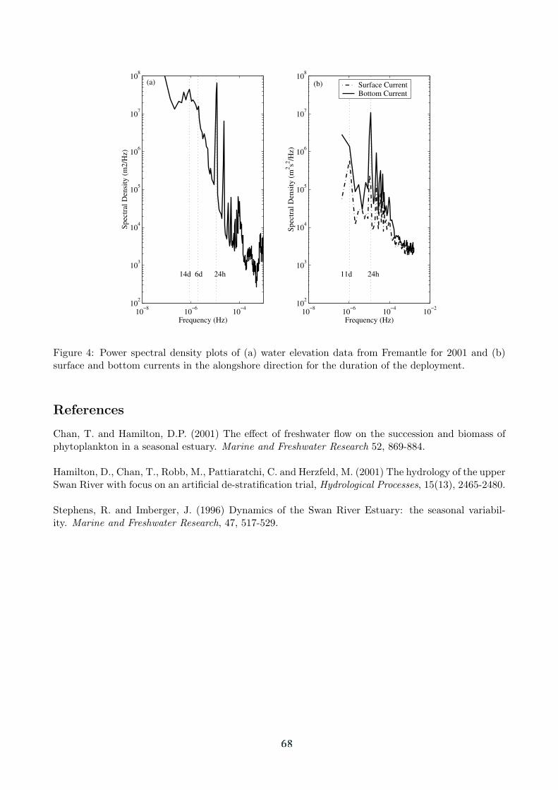
10−8

10−6

10−4

102

103

104

105

106

107

108

Spec

tral

Den

sity

(m

2/H

z)

Frequency (Hz)10

−810

−610

−410

−210

2

103

104

105

106

107

108

Spec

tral

Den

sity

(m

2 s2 /Hz)

Frequency (Hz)

Surface CurrentBottom Current

14d 6d 24h 11d 24h

(a) (b)

Figure 4: Power spectral density plots of (a) water elevation data from Fremantle for 2001 and (b)surface and bottom currents in the alongshore direction for the duration of the deployment.

References

Chan, T. and Hamilton, D.P. (2001) The effect of freshwater flow on the succession and biomass ofphytoplankton in a seasonal estuary. Marine and Freshwater Research 52, 869-884.

Hamilton, D., Chan, T., Robb, M., Pattiaratchi, C. and Herzfeld, M. (2001) The hydrology of the upperSwan River with focus on an artificial de-stratification trial, Hydrological Processes, 15(13), 2465-2480.

Stephens, R. and Imberger, J. (1996) Dynamics of the Swan River Estuary: the seasonal variabil-ity. Marine and Freshwater Research, 47, 517-529.

69

Salinity Effects of Riverine Diversions to Barataria Basin, aBar-Built EstuaryDONGHO PARK, MASAMICHI INOUE, AND WM. J. WISEMAN, JR.

Coastal Studies Institute and Department of Oceanography and Coastal Sciences, School ofthe Coast and Environment, Louisiana State University, Baton Rouge, LA, 70803, USA

Barataria Basin is located immediately west of the birdfoot delta of the Mississippi River. It includesa large bar-built estuary, marshes, and upland swamps. Land loss due to subsidence and exacerbatedby human activity is a chronic and important problem in coastal Louisiana. One potential solution tothis problem is diversion of river water and its associated nutrients and sediments from the MississippiRiver into the adjacent marshes. This promotes the maintenance of the marsh. The added freshwater,though, alters the region in which commercially important living marine resources, e.g. oysters, canprosper. In order to assess the affect of river diversions, a circulation model was developed.

The waters of Barataria Basin range from 1 to 3 meters in depth. The dominant diurnal tides at themouth of the estuary have a range of approximately 60 cm during tropic tidal conditions. The shearassociated with the tidal currents effectively mixes the shallow water column. Additional mixing isdue to wave-bottom interactions and Langmuir circulations. Thus, a vertically integrated model wasassumed, as a first approximation to the estuarine dynamics. The model included baroclinic pressuregradients. It was forced at the sea surface with observed wind and precipitation and with computedevaporation. Precipitation over the marsh was converted to runoff using a hydrologic modeldeveloped for this study. Open boundary conditions in the coastal ocean, water level and salinity,were derived from observed conditions at the mouth of the estuary. The model grid size was 100 m.A high-resolution advection scheme was coded to replace the traditional centered difference scheme.When compared to results from a previous version of the model, with a larger grid size of 463 m, thepresent model performs significantly better in terms of its ability to model the observed tidalpropagation up the complicated channels of the estuary (Figure 1).

The model was run once without diversion structures and once with the inclusion of two existingdiversion structures that were forced to run at their maximum design discharge rates as well asfreshwater inflow from the Gulf Intracoastal Waterway, a navigation canal that traverses the upperreaches of the Basin. Differencing the solutions from the two runs permitted the effect of thefreshwater diversions to be assessed in terms of water levels, salinity distributions, and transports. Theecologically important variable, salinity, was measurably altered by the active diversions. Within theconvoluted tidal creeks and marshes near the diversion outfalls, salinities decreased by as much as 5.In the middle reaches of the estuary, salinities decreased by 2. The lower reaches of the estuary wererelatively unaffected due to both dilution and effective flushing driven by the wind and tides(Figure 2). Salinities could not, of course, be significantly lowered in the nearly fresh regions of theupper estuary.

Issues remain to be resolved with the open boundary conditions and regarding possible three-dimensional effects in the deeper regions of the estuary. When compared to observed salinities, themodel output did not adequately track strong salinity intrusions. The salinities at the open boundarywere inferred from salinities observed at the mouth of the Basin and, thus, known to be in error.Furthermore, while the waters of the Basin are generally shallow, the deep passes connecting theestuary to the coastal ocean and the coastal ocean proper are known to be strongly stratified. Themodel does not allow saline intrusions along the bottom near the mouth of the estuary. The estuaryincludes a boat channel that extends from the deepest pass northwards to the Intracoastal Waterway.This channel is also capable of supporting stratified shear flows. Nevertheless, over most of the Basin,where the assumptions of the model are believed to be valid, the dispersion of salinity is thought to bequalitatively reproduced.

70

Figure 1. Model grid. Each dot represents a model grid point. The sources of controllable freshwater input areindicated by black squares. The stations indicated by black circles run along the Barataria Waterway, a dredgedship channel, and are sampled to produce figure 2.

Figure 2. Time-distance plot of the salinity difference between model runs with and without controllablefreshwater discharges. Contour interval is 0.5.

71

Observations of Bathymetric and Curvature Effects on theTransverse Variability of the Flow in a Coastal Plain EstuaryROSARIO SANAY AND ARNOLDO VALLE-LEVINSON

(Center for Coastal Physical Oceanography, Old Dominion University, Norfolk, VA 23508,USA )

1. IntroductionHydrographic and horizontal velocity measurements were used to describe the tidal and subtidal flowaround a headland over laterally varying bathymetry in the lower James River, Virginia. Threeshipboard surveys were conducted throughout semidiurnal cycles along two parallel cross-estuarytransects in the vicinity of the headland. In general, the tidal forcing, the river discharge and the windconditions were different for each cruise. Both tidal and subtidal signals of the along-channel velocitycomponent showed lateral variability related to the bathymetry and curvature. The subtidal flow wasup-estuary over the shoals and closest to the headland two-layer estuarine circulation developed in thechannel. In every cruise, the subtidal velocity data depicted an anticyclonic gyre over the transectclosest to the headland, likely in response to friction and curvature effects. The lateral flow showedpatterns that differed from the secondary circulation expected from curvature effects only in one of thethree cruises. This might be explained by the counteracting effects of the lateral density gradients andwind forcing observed.

Fig 1. Map of the study area and the cruise track (white lines) of the ship borne ADCP surveys. The bathymetryis denoted by tones of gray (dark means deeper). The CTD-stations are indicated by asteriks

2. Study areaThe James River Estuary is the southern most tributary to the Chesapeake Bay. The transition areabetween these two systems is characterized by abrupt lateral bathymetry changes associated withnavigational channels and shoals and by a strong coastline bend associated with a prominent headland,

72

Newport News, located in the north. The across-channel depth ranges from 3 m (Hampton Flats) to17m (navigation channel). The radius of curvature of the bathymetry in the area is 10 km. This system isa typical example of a partially stratified coastal plain estuary forced mainly by river discharge andtidal forcing. Mean annual river discharge recorded at Richmond, Virginia ranges from 500 m3 s-1 inMarch to 80 m3 s-1 in August (Wood and Hargis, 1971). Both, tidal elevation and tidal current aremostly semidiurnal, where M2, N2 and S2 are the more energetic (M2 represents 80 % of the total tidalenergy). The interaction among them generates fortnightly and monthly variability in the tidal current(Valle-Levinson et al., 2001). Wind forcing and remote forces (e. g. wind-driven mean sea levelfluctuations in the Chesapeake Bay) may also play an important role in the dynamics. The windforcing is primarily from the northeast, northwest and southwest.

3. Data collectionThree shipboard surveys were conducted along a rectangular track seaward of the Newport Newsheadland (Fig. 1). The surveys took place throughout two secondary spring (Feb 2001, May 1998) andone secondary neap (March 2001) semidiurnal cycles. Each survey sampling consisted of continuousvelocity measurements and density profiles.

The current velocity profiles were obtained with an acoustic Doppler current profiler (ADCP) inconjunction with a Trimble differential global positioning system (DGPS). The ADCP was mountedpointing downward on a catamaran and towed from the starboard side of the ship along the track. Theship steamed at 2.5 m s-1, allowing the track (8 km) to be repeated 11 times through out the totalperiod of sampling on each cruise. Density profiles were sampled with a SEA-BIRD CTD at stationsindicated in Figure 1.

The tidal and subtidal signals were separated from the current velocity observations by usingsinusoidal least squares fitting techniques to semi-diurnal and quarti-diurnal harmonics. The velocityfields were rotated such that the along-channel component was aligned to the maximuminflow/outflow. The subtidal signal of the data includes the effects of tidal rectification, wind,baroclinic gradients and curvature effects. The density data were subject to the same fit analysis as thecurrent velocity profiles.

Hourly wind velocity data were obtained from NOAA at stations CBBT , Kiptopeke and SewellsPoint. Daily streamflow data were obtained from USGC at station Richmond.

4. Results

Along Channel Flow

Despite the fact that the three cruises took place under different wind, river discharge and tidal forcingconditions, the general structure of the along channel mean flow was quite similar for all the cruises.It exhibited a transverse variability related to the bathymetry (Fig. 2). It featured two-layer circulationover the channels (main and secondary channels) in both transects. This feature was consistent withKasai et al. (2000), in the sense that 2-layer estuarine circulation was developed at the deepest part ofthe estuary. Over the shoal, the mean-flow was up-estuary for the transect closer to the headland andweak down-estuary mean flow at the eastern transect. These results might be attributed to the non-linearities of the dynamics of tidal flow as indicated by the theoretical results of Li and O’Donnell(1997). They found that the vertically integrated exchange flow was correlated with topography, as anet inflow occurred over the shoals and net outflow in the channels.

The strongest mean outflow in all the cruises was found at the upper layer of the main channel asexpected from reduced friction effects there.

73

a) b) c)

The semidiurnal tidal amplitude of the along-estuary velocity exhibited transverse variability related tothe bathymetry. Maximum velocity amplitudes were located on the upper layer of the main channel,decreased over the shoals, and then increased slightly on the upper layer of the secondary channel.Bottom friction effects were evident in decreasing the amplitudes of the currents near the bottom andover the shallow areas. The semidiurnal phase of the along-channel velocity also showed a lateral andvertical variability, with the shoals and bottom part of the channels leading the rest of the cross-sectionarea by about 20 degrees or 40 minutes. The phase lag may be due by the combined effects of frictionand inertia. The tidal features at the shoals (amplitudes and phase) generated lateral gradients of thealong-channel flow that induced convergence processes. These features were consistent with otherstudies (Valle-Levinson et al., 2000, Li and Valle-Levinson, 1999).

Nonlinear effects also were explored by the M4/M2 tidal amplitude ratio. This ratio features maximumvalues at the shallowest part of each transects, which was more evident on the western transect.

Lateral Channel Flow

The lateral mean flow for all the cruises featured convergence and divergence areas associated withthe shoals and shoulders of the main channel.

In general, the lateral flow at the eastern transect showed mean flow outward the bend on the upperlayer and mean flow inward the bend on the lower layer. At the western transect the lateral circulationwas mostly outward the bend at southern part. One of the cruises showed some differences with thisgeneral lateral flow. This might be due to counteracting effects of the lateral density gradients andwind forcing observed.

The theoretical strength of the secondary circulation due to the channel curvature and Coriolis effectswere obtained by using scaling analysis provided in Geyer (1993) and Seim and Greeg (1997). Thisanalysis suggested that curvature effects (0.03 m s-1) dominated over Coriolis effects (0.002 m s-1).This result was consistent with the evaluation of the Rossby number, which was bigger than one in thecomplete domain. The across-channel baroclinic force also was at least one order of magnitude lessthen the centrifugal force during the periods of sampling.

The radius of curvature during ebb was smaller than during flood, consequently the centrifugal forceduring ebb drove stronger lateral flow than during flood. This feature explains some of the diferencesof the mean lateral circulation between eastern and western transect.

Fig 2. Subtidal current for the three surveys at three different water levels, surface (black arrows), below thesurface (dark gray arrows) and near bottom (light gray arrows). a) May 98 survey, b) February 2001 surveyand c) March 2001 survey. Maximum mean flow was ~ 20 cm s -1.

74

5. SummaryThe along channel tidal and subtidal flow exhibited transverse variability related to the bathymetry.The the flow over the shoals featured minimum tidal amplitudes, and net mean inflow. The flow overthe channels showed maximum amplitudes of the tidal amplitudes and the mean flow showedestuarine circulation. The tidal phase difference between the shoals and channels and transverse shearsof the along channel flow caused convergence and divergence processes. These results were consistentwith observational studies reported in the literature.

The lateral circulation was dominated by curvature effects. Coriolis effects and baroclinic pressuregradients were one order of magnitude less than the curvature term. The centrifugal force during ebbdrove stronger lateral flow than during flood. In every cruise, the subtidal velocity data depicted ananticyclonic gyre over the transect closest to the headland, likely in response to friction and curvatureeffects.

References

Geyer , W. R., Three-dimensional tidal flow around headlands. J. Geophys. Res., 98: C1, 955-966, 1993.

Kasai A., A. E. Hill, T. Fujiwara, and John H. Simpson, Effects of the earth’s rotation on the circulation inregions of frshwater influence, J. Geophys. Res., 105: C7, 16961-16969, 2000.

Li and O’Donnell, Tidally driven residual circulation in shallow estuaries with lateral depth variation. J.Geophys. Res., 102: C13, 27915-27929, 1997.

Li, C. and A. Valle-Levinson, A two dimensional analytical model for a narrow estuary of arbitrary lateral depthvariation: The intratidat motion. J. Geophys. Res., 104: C10, 23525-23543, 1999.

Seim, H. E., and M. C. Greeg,The importance of aspiration and channel curvature in producing strong verticalmixing over a sill, J. Geophys. Res., 102: C2, 3451-72, 1997.

Valle-Levinson, A., C. Li, T.C. Royer and L. P. Atkinson, Flow patterns at the Chesapeake Bay entrance, Coast.Shelf Res., 18, 1157-1177, 2001.

Valle-Levinson et, A., C. Y. Li, K. C. Wong, and K. M. M. Lwisa, Convergence of lateral flow along a coastalplain estuary, J. Geophys. Res., 105: C7, 17045-17061, 2000.

��

� ��

��

� ��

�� !""#$% &�� '( �� %�% ��

!"""$�) �� *��) �� +�� % &�� % ,� �� -�� +�� .�� +�� -�� #�%

x

y

114mm

45mm

U

yU

Um

1

Ux,

h =20mm1

(�� #/ 0��/ �� -��% 1��/ �� - � �� %

&�� "� ��

�� 2 �� 2 �� 3 "

�� 2 �� 2 �� 2 �� 3 ��

�2 ��

��

�� 2 �� 2 �� 2 �� 3 ��

2 ��

�#�

�� 3 �2 � �� ) � 3 �� 4��.� �� Æ��%

� � � ��

&�� .�� +�� %�% �� #567$� �� 8��

�� %�% �� #55#$�% &�� .��% &�� )�� +� �) � �� %

9�8�� .� �� %

��

9�� -�� ) �� ) �� % ,� �� 3 " �� 3 "� �� #56:$�% &�� *�� /

�

�

��

3

�!

�� 2 �� $�� 3

� �� $�

;�� 3 �� !�

��

<�� .�� - � �� -�� #�% &�� ) ��)�� %�%�� #55#$�%

�� !%#% ' �� *�� *�� $�� % <�� % =��)�� $�� !�%

� ��

�� 3 " �� +�� .� �� 3 "�"">�% =��) �� 8�� % ,� �� '( ��) �� ) �� -�� % ,� �� ) �� ) �� % &��

�� /

�� 3

#

!�#� ��? �:�

�� 8�� ) �� #�� % @�� % &�� .� �� 8�� .� ? ) �� 4�� %

(�� !/ &� ��/ �� 3 #� �� ? �� 3 #�"" � ��) ? �� 3 "�A"�� ? �� 3 "�!A ��% B�� / �� 3 #""� �� ? ��% 4�� !�A�� !�A��%

,� �� 8�� ) �� ? ) �� .�� -�� % �� ) ��) ��8�� .�� %

&� �� +�� -�� -�� # �� .� �� ? 3 ?��% �� -�� !% ,� �� A�� A�� !%# �� !%! ��%�% �� % &�� 8�� .� �� + �� % @��) ��-�� % =��) ��-�� .� �� %

(�� :/ C�� *�� ? �� 3 "�A �� ;"� �� 3 #� � �� 3 6"� ��% 9�� 3 " �� 3 "�>A �� %

,� �� .� �� +� �� 0�� *�� % ,� -�� : � �+� � �� *�� ) �%�% �� 3 �) �� !%# �� !%!% (�� -�� % 0��) �� ) �� -�� :% &�� 8�� ) ��) ��) ��8��) ��%�%

� � � � ��

B��) @%) B��) 1%) @�� ) '% �� ' ��) D%) '� �Æ�� '( ��) �� ) ��) #"A�#!5) !""#%

4��) E% =%) ��) F% =% �� G��) 1% �%) �� ) �� ) ��) #:>"�#:6#) #55#%

C��) 0% F%) <� �� % C�� #% �� *�� ) �� !��) ��) #5A�!#6) #56:%

&��) �%) '��) &% �� ,��) =%) �� ) "�� #�� #��) $$) ##!5�##:6) #567%

&��) �% (%) ��%��&�� '�� '��'�� ( )�(�) F% �� )�� H��) 4��) B��) !"""%

79

Modeling the salt wedge dynamics of the Itajaí EstuaryH. JACOB VESTED

(DHI Water & Environment – Agern Alle 11, DK-2970 Hørsholm, Denmark , [email protected])

CARLOS SCHETTINI

((Center of Earth and Marine Sciences - CTTMar, University of Vale do Itajái - UNIVALI, R.Urugai 458, C. P. 360, Itajai - SC - Brasil 88302 -202, [email protected])

OLE SVENSTRUP PETERSEN

(DHI Water & Environment,, [email protected])

1. IntroductionThe Itajaí Estuary is located in Southern Brazil in the state of St. Catarina. It can be characterised as amicro-tidal estuary, where the average tide at the mouth is about 0.8 m. The average river discharge isabout 250 m3.s-1 and more than 1000 m3.s-1 during high flow. The estuary is highly stratified and asalt-water wedge is observed most of time. During average river discharge conditions the salt intrusionreaches about 18-20 km upstream, and the maximum observed salt wedge intrusion ever was 32 km.At a flow rate of 500-800 m3.s-1 a freshwater plume is well developed off the river mouth and at 1000-1200 m3.s-1 all salt is washed out of the estuary. The river plume extends several kilometres offshoreduring high flow, inducing complex patterns in the near shore coastal circulation.

Modelling the salt-water wedge and fresh water plume dynamics of Itajaí estuary poses severaldifficulties. It requires a high accuracy three-dimensional hydrodynamic model coupled with a salinitytransport model. Further the model must be able resolve in details the river part, the estuary itself aswell as the open sea where strong gradients occur both horizontally as well as vertical. This isdemanding both from a numerical accuracy point of view as well as from limiting the computationaltime of simulations. The application of a hydrodynamic model with a variable and unstructured grid isapplied in order to reproduce the extensive observation of the salt-water wedge under different flowconditions while at the same time analyse the applicability of the model for this type of estuary.

2. The numerical modelThe model solves the three-dimensional shallow water equations, using a hydrostatic approximation,coupled to transports of salinity and heat through an equation of state. The free surface is describedusing vertical sigma co-ordinates and solution of a generalised wave equation (Lynch and Werner,1991). The model further includes a full 3D k-epsilon model. The numerical solution is based onstandard Galerkin linear finite elements using an unstructured mesh with linear triangles horizontallyand a surface and bottom adaptive layered discretisation vertically (Burchard and Petersen, 1997).Time stepping is made using a semi-implicit method, where the gravity wave terms in the waveequation and the vertical terms in the momentum and transport equation are solve implicitly.

3. Model resultsThe model set-up is shown in Figure 1, and covers the coastal area in the vicinity of the estuary mouth,the estuary and the river up to 35 km from the mouth. The resolution varies from 500 m in t coastalarea to 100 m in the river section. The vertical resolution follows the bathymetry and is discretisedusing 10 layers, with finest resolution near the surface. Boundary conditions are observed water levelsat the ocean and the river discharge at the inland boundary. The simulations cover a 2 week period.The coastal area is included in order to accomodate the partial mixing of estauarine water in thevicinity of the mouth, and thereby establish a more accurate inflow salinity.

80

Figure 1: Bathymetry and unstructured mesh of the Itajai Estuary

The simulated results are compared with water level gauges in 3 stations and salinity transects of thesalt-water wedge for different levels of the river run-off.

In Figure 2 is shown time series of computed and observed elevations at an upstream station for atypical spring and a neap period. The tides in the estuary have a significant quarterjournal component.Further, it is characteristic that the tidal wave proceeds nearly undistorted up through the estuary.

Figure 2: Modelled and observed water levels 35 km from the estuary mouth.

In Figure 3 and 4 are shown transects of the salinity up through the estuary at low and high tide. Theuppermost tip of the intrusion is relatively stationary at 20 km, while the 30 PSU contour travelsbetween 5 and 10 km during the tide. It is further evident that the height of the wedge increases duringraising tide. The length of the saline wedge represents a relatively delicate balance between thebaroclinic pressuregradients and the friction and vertical mixing along the interface.

81

Figure 3: Observed an modelled salinity distribution at low tide

Figure 4: Observed and modelled salinity distribution at high tide

4. SummaryThe study has shown the usefulness of the model to in applications to estuarine flows. As a first step ishere discussed the effects of tides, river runoff and salinity intrusions. It is however planned, toinclude sediment and water quality related parameters at a later stage.

82

References

Lynch, D. R. and Werner , F. E. Three-dimensional hydrodynamics on finite elements. Part II: Non-linear timestepping model. International Journal for Numerical Methods in Fluids,12,507-533(1991).

Burchard, H. and Petersen, O. Hybridization between σ- and z-coordinates for improving the internalpressure gradient calculation in marine models with steep slopes. International Journal for NumericalMethods in Fluids, 25, 1003-1023, (1997).

��

�� !��

� ��

�� !�� "#$%%&' �� !�� "#$$(&� )�� "� ��&*� �� +�� "#$$#& �� *� ,�� -�� "#$$.&�� !�� "#$$$&� ��

/�� 0�� )�� 1�� 2� � �� 345- ��

� � ��

�� !�� 6�� -�� "#$%.&*� �� 3 7�� 7 �� 5�� !�� 6�� # �� $� �� 8� � ��

�� 2� �� 9: � �� 3 �� #9;; �<1 3�� 4�� 5�� -�� 345-* �� 345- �� # �� 9: �� 4�� !�� 5�� 3�� =�� -�� !53=-* �� 5�� /�� > �� !53=- �� ?�� * �� 0�� 8 ��

%@

�� #� �� ?�� 3�� +��

�� 345- �� #; �� )�� 0�� 0�� "#$$;&� �� A�� !�� "#$$$& � ��

�� B��

( � � �� #*

�� *� �� * ��

�� )�� A�� 1�� )�� -4�* �� C

��* B ��*��D *� �9*

�� )��* � �� B; �� )��;* �� )��* �� 6�� "#$$$&*�

� � ��

E�� % �� #(�;%�;# �� % �� #:�;%�;# �� 998�@�99.�@* �� !��6�� #: �� 9; �� :; �� 2� �� #�*�

4�� A�� #�8 �� 998�@:�998�(:� �� 0�� A�� 998�8�998�.:* �� 998�% �� A�� ;�: �� #�*�

�� )��? �� *� ,�� ?�� 998�% �� 99.�@:�

%(

−50−40−30−20−1001020304050

226.3 226.4 226.5 226.6 226.7 226.8 226.9 227 227.1 227.2 227.3

2

4

6

8

Time / decimal day

Hei

ght a

.b. /

m

0

0

0

0

−10

−20

10

20

10

20 10

−10 −20

−40

0

−10

−20 10

1010 20

10

cms−1 a

226.3 226.4 226.5 226.6 226.7 226.8 226.9 227 227.1 227.2 227.37

8

9

10

11

226.3 226.4 226.5 226.6 226.7 226.8 226.9 227 227.1 227.2 227.3−2

−1.5

−1

−0.5

0

Time / decimal day

∆ ρ

/ kg

m−

3

Wat

er le

vel /

m b

−20

−10

0

10

20

226.3 226.4 226.5 226.6 226.7 226.8 226.9 227 227.1 227.2 227.3

2

4

6

8

Time/ decimal day

Hei

ght /

m

c cm2s−2

�� #C -�� 9: � �� 5�� /�� #(�#:�3�� 9;;#C �� * �� *� �� A�� *�� * �� * �� )�� ,�� #;�� 345- ��

�� )�� ?�� ;�9:� <�� 998�:�998�% �� 99.�99.�@* �� /�� Æ�� A � �� A��

�� )�� #�*� �� !�� "#$$$&*� F� �� )�� 9; ��

%:

�� 2� �� )�� :?#; ��

�� )�� ( � �� 998�:�998�.*� 5�� )�� B; �� -4� �� * �� A�� 1�� 4�� 998�% �� 99.�� )��

,�� )�� #9�9; �� * �� %�#; �� *� �� C �� ?��

��

�� !�� " �� #��$

�� %& �� #�� '��

� � � � ��

+�� =� 5�� C � �� @$�(:� #$$#�

�� -� �� G� ,� !�� =�� ##;.�##9.� #$%%�

�� 3�� /� <�� 4� )�� <��?�� #$�@.� #$$;�

�� )� +� �� 6�� 3� �Æ�� ?�� ..@�..:� #$$$

-�� <�� F� �� C H��?�? �� ?�� !� 8$�%%� #$$.�

-�� 4� �� " �� #��$ � �� %��& �� G�� 6�� !�� 5�� #$%.�

!�� G�� G� <� !�� G� =� /�� F� �� ?�� E�� " ��

�� '�� @;#�@#9� #$$(�

!�� =� �� !� =�� G� )� /�� F� �� -��!�� , �� (�� )*� #$:;�.;� #$$$�

%8

87

"Stress calculations from PIV measurements in the bottomboundary layer"THOMAS OSBORN

(The Johns Hopkins University, 3400 N Charles Street, Baltimore, MD 21218, USA,[email protected])

W.A.M. NIMMO SMITH, W. ZHU, L. LUZNIK, AND J. KATZ

(The Johns Hopkins University, 3400 N Charles Street, Baltimore, MD 21218, USA)

1. IntroductionTurbulence measurements with a Particle Image Velocimetry (PIV) system were made in the bottomboundary layer of the coastal ocean. The submersible PIV system was deployed in water 12m deepabout 5km off the New Jersey coast. The system consisted of two 12-bits-per-pixel, 2K x 2K digitalcameras, operated simultaneously. Each camera imaged a 40cm x 40cm vertical plane aligned with thecurrent which was illuminated by a light sheet. A pair of flash-lamp pumped, dye lasers at the surfacegenerated double pulses, which were transmitted through optical fibers to submerged probes thatproduced the light sheets. Computers recorded the double exposure images from each frame, but ahardware-based 'image shifter' displaced the exposures relative to each other. Naturally occurringparticles - sediment, plankton or other material - were used as tracers.

Calculations of the turbulent stress, in the presence of waves, are possible by using second orderstructure functions. This approach is an extension of the approach of John Trowbridge(Trowbridge,1998; Shaw and Trowbridge, 2001).

2. MeasurementsDetails of the measurement system are outlined in Bertuccioli et. al. (1998), Doron et. al. (2001) andNimmo Smith et. al. (2002). Further information about the system along with some animations of thedata are available on our web site http://cloudbase.me.jhu.edu/.

Figure 1. Two PIV images taken with the same camera 0.9 secs apart. The in plane velocities are shown asvectors while the vorticity is color coded with the scale along the side. Note especially the two vortices whichare propagating to the right with the mean flow.

88

3. Stress CalculationThe Reynolds’ stresses arise from the decomposition of the velocity field into mean and fluctuatingparts. It is convenient to separate the fluctuations into two types, turbulence which causes mixing anddissipation and waves which generally cause neither. Writing the horizontal velocity component, u ,asa sum of the mean, u , the wave motion, u , and the turbulent fluctuations, ′u .

u u u u= + + ′˜ .

The same notation for the vertical component yields:

w w w w= + + ′˜ .

The Reynolds stress is the product of the fluctuations:

( )( ) ( ˜ ) ( ˜ )u u w w u u w w− − = + ′ ⋅ + + ′ .

( ˜ ) ( ˜ ) ˜ ˜ ˜ ˜u u w w uw u w uw u w+ ′ ⋅ + ′ = + ′ ′ + ′ + ′

( )( ) ˜ ˜ ˜ ˜u u w w uw u w uw u w− − = + ′ ′ + ′ + ′

The wave turbulence cross terms uw′and ′u w are usually assumed to average to naught but aspointed out by Alex Hay (per. com.), the presence of a solid boundary can convert horizontal wavemotion into vertical motion with spatial scales associated with the topographic features. We willreturn to this point later but for now will adopt the usual approach and assume these terms do notcontribute to the correlation giving the desired result;

< − − >=< ′ ′ >( )( )u u w w u w

Now, if the measurement axes are inclined (as they almost certainly will be) then the measuredvelocity components are a combination of both the horizontal and vertical components.

U u w= ⋅ + ⋅cos sinθ θ

W u w= − ⋅ + ⋅sin cosθ θ

( ) ( ) ( ˜ ) ( ˜ )(cos sin )

( ˜ ) ( ˜ ) cos sin

U U W W u u w w

w w u u

− ⋅ − = + ′ ⋅ + ′ − +

+ ′ − + ′( ) ⋅

2 2

2 2

θ θ

θ θ

for small θ , cosθ → 1 and sinθ θ→ and thus:

( ) ( ) ( ˜ ) ( ˜ ) ( ˜ ) ( ˜ )U U W W u u w w w w u u− ⋅ − ≅ + ′ ⋅ + ′ + + ′ − + ′( )2 2 θ

near the ocean floor, the horizontal orbital velocity component is larger than the vertical and muchlarger than the turbulent fluctuations

( ) ( ) ˜U U W W u w u− ⋅ − ≅ ′ ′ + 2θ

and the latter term overrides the desired measurement.

Trowbridge (1998) introduces, and Shaw and Trowbridge (2001) further develop, a technique forovercoming the wave contamination problem by using measurements from two sensors spaced apartby an amount that is large compared to the stress containing eddies but small compared to thewavelength of the surface waves. The application of this technique is slightly different for PIV databecause of some of the innate characteristics of the data i.e., the strong alignment of the velocitycomponents measured at different locations.

The second order structure function is the covariance of the velocity differences.

D x r t u x t u x r t u x t u x r tmn m m n n( , , ) ( ( , ) ( , ))( ( , ) ( , ))r r r r r r r r

=< − + − + >

where the brackets <> denote some appropriate average.

89

D x r t u x t u x t u x r t u x r t

u x t u x r t u x r t u x tmn m n m n

m n m n

( , , ) ( ( , ) ( , ) ( , ) ( , )

( , ) ( , ) ( , ) ( , ))

r r r r r r r r

r r r r r r=< ⋅ − + ⋅ +

+ ⋅ + + + ⋅ >

If the velocity field is steady, homogeneous and reflexive symmetric

D x r u x u x u x u x rmn m n m n( , ) ( ) ( ) ( ( ) ( )r r r r r r r

= < ⋅ > − < ⋅ + >2 2

D x r u x u x R x rmn m n mn( , ) ( ) ( ) ( ( , ))r r r r r r

= < ⋅ > ⋅ −2 1

Thus, the value of D x rmn( , )r r

increases from 0 at rr = 0 , to 2 < ⋅ >u x u xm n( ) ( )

r r when

rr exceeds the

scale of the stress containing eddies.

As long as rr is less than the scale of the surface waves, the wave contamination problem is avoided.

The best way to see this point is to expand the second order structure function for U and W to seehow the wave orbital motion and the inclination of the measurement frame enter into the result. Forconvenience we modify the notation as follows:

rx is denoted by xi since we are considering locations

along a horizontal axis. For our data we are interested in values of rr that are parallel to the horizontal

(x axis) so rr is denoted by rj . U and the various u ’s denote horizontal velocity components while

W and the w ’s denote vertical components, subscript i denotes the location xi and subscript j denotes

the location x ri j+

d t D x r t U x t U x r t W x t W x r tij i j i i j i i j( ) ( , , ) ( ( , ) ( , ))( ( , ) ( , ))= =< − + − + >13

r r

d U U W Wij i j i j=< − − >( , )( )

( , )( , )( ˜ ) cos ( ˜ ) sin

( ˜ ) cos ( ˜ ) sin

( ˜ ) sin ( ˜ ) cos

( ˜ )U U W W

u u w w

u u w w

u u w w

u ui j i j

i i i i i i

j j j j j j

i i i i i i

j j

− − =+ ′ ⋅ + + ′ ⋅

− + ′ ⋅ − + ′ ⋅

•

− + ′ ⋅ + + ′ ⋅

+ + ′

θ θ

θ θ

θ θ

⋅⋅ − + ′ ⋅

sin ( ˜ ) cosθ θj j j jw w

The turbulent terms give similar results to what we found before:

( ) (cos sin ) ( ) (cos sin )

cos sin cos sin cos cos

cos sin sin sin

′ ⋅ ′ ⋅ − + ′ ⋅ ′ ⋅ −

− ′ ⋅ ⋅ + ′ ⋅ ′ ⋅ ⋅ − ′ ⋅ ′ ⋅ ⋅

+ ′ ⋅ ⋅ + ′ ⋅ ′ ⋅ ⋅

u w u w

u u u u w

w u w

i i i i j j j j

i i i i j i j i j i j

i i i j i i j

2 2 2 2

2

2

θ θ θ θ

θ θ θ θ θ θ

θ θ θ θ −− ′ ⋅ ′ ⋅ ⋅

+ ′ ⋅ ′ ⋅ ⋅ − ′ ⋅ ′ ⋅ ⋅ − ′ ⋅ ⋅

+ ′ ⋅ ′ ⋅ ⋅ − ′ ⋅ ′ ⋅ ⋅ + ′ ⋅ ⋅

w w

u u u w u

u w w w w

i j j i

j i j i j i i j j j j

i j i j i j i j j j j

) cos sin

cos sin cos cos cos sin

sin sin cos sin cos sin

θ θ

θ θ θ θ θ θ

θ θ θ θ θ θ

2

2

With the PIV system θ has the same value at both locations. The digital cameras are leveled andaligned, relative to each other across both sheets, to within 1 pixel (1 pixel is 1/2048 of the verticalwindow dimension, nominally 0.5 m) in the nominal 1.5 m maximum separation. Hence, thedifference in angle between two points (on separate light sheets) is 1/6144 radians or 0.01 degrees.Combining that with the small angle expansion of the trigonometric functions the turbulent terms (toorder θ and written as correlations) are:

( ) ( ( , )) ( ) ( ( , ))

( ( , )) ( ( , ))

( ( , ))

′ ⋅ ′ ⋅ − + ′ ⋅ ′ − + −

− ′ ⋅ ⋅ − − ′ ⋅ ⋅ − + −

+ ′ ⋅ ⋅ − + ′

u w R x r u w R x r r

u R x r u R x r r

w R x r w

i i i j j j i j j

i i j j i j j

i i j j

1 1

1 1

1

13 13

211

211

233

2

θ θ

θ ⋅⋅ ⋅ − + −θ ( ( , ))1 33R x r ri j j

The wave terms are:

˜ cos ˜ cos ˜ sin ˜ sin ˜ sin ˜ cos ˜ sin ˜ cosu u w w u w u wi i j j i i j j i i i i j j j j⋅ − ⋅ + ⋅ − ⋅{ }• − ⋅ + ⋅ + ⋅ − ⋅{ }θ θ θ θ θ θ θ θ

Since the alignment of the two cameras means the orientation of the velocity measurements is thesame at all measurement points, terms like ˜ cos ˜ cosw wi i j jθ θ− have values on the order of

90

( ˜ ˜ )cos˜

˜w ww

xr kwri j j j− =

∂∂

=θ (where k is the wave number of the surface wave in the x direction)

rather than ˜ (cos cos ) ˜ ( )w wθ θθ θ

1 222

12

2− =

−. (The latter value is appropriately used in

Trowbridges’s analysis because his two sensors are not necessarily collinear.) Similarly,

( ˜ sin ˜ sin )˜

˜u uu

xr kuri i j j j j⋅ − ⋅ =

∂∂

⋅ =θ θ θ θ . For such terms we will use the shorthand notation of the

form ∆ ˜ ˜ ˜u u uij i j= − .

The wave terms can now be rewritten:

( ˜ ˜ ) ( ˜ ˜ ) ( ˜ ˜ ) ( ˜ ˜ ) ( ˜ ) ( ˜ ) ˜ ˜u u w w u u w w u w u w Oi j i j i j i j ij ij ij ij− + − ⋅{ }• − − ⋅ + −{ } = ⋅ + ⋅ + ⋅ + [ ]θ θ θ θ θ∆ ∆ ∆ ∆2 2 2

Thus, the wave contamination of the stress estimate, which used to be a term on the order of u2 ⋅θ , isnow of the order ( ˜ )∆uij

2 ⋅θ . The effect is smaller by a factor of ( )kr 2 , which is on the order of 10-3 for

a wave of 6 seconds period and a separation of 1.5 m.

Now following the normal assumption that the wave and turbulent fluctuations don’t correlate, we canwrite

d U U W W

u w R x r u w R x r r

u R x r u R x r r

wij i j i j

i i i j j j i j j

i i j j i j j

i

=< − − >=

′ ⋅ ′ ⋅ − + ′ ⋅ ′ − + −

− ′ ⋅ ⋅ − − ′ ⋅ ⋅ − + −

+ ′ ⋅( , )( )

( ) ( ( , )) ( ) ( ( , ))

( ( , )) ( ( , ))

1 1

1 1

13 13

211

211

2

θ θ

θθ θ

θ θ θ

⋅ − + ′ ⋅ ⋅ − + − +

⋅ + ⋅ + ⋅ +

+( ( , )) ( ( , ))

( ˜ ) ( ˜ ) ˜ ˜ ( )

1 1332

33

2 2 2

R x r w R x r r

u w u w O

i j j i j j

ij ij ij ij∆ ∆ ∆ ∆

The structure function begins at zero with no separation and rises to (minus) twice the stress as theseparation exceeds the scale of the stress containing eddies, as long as the waves are of much largerscale than the turbulent eddies. Otherwise, if the spatial scale becomes too large,

then∆u u uu

xr kurij i j j j= − =

∂∂

=( ˜ ˜ )˜

˜ is no longer small compared to ′u and the whole wave

contamination problem resurfaces.

Acknowledgments: This work has been supported by the Office of Naval Research and the National ScienceFoundation.

References:

Bertuccioli, L., G.I. Roth, T.R. Osborn and J. Katz, Turbulence measurements in the bottom boundarylayer using particle image velocimetry. Journal of Atmospheric and Oceanic Technology 16, 1635-1646, 1998.

Doron, P., L. Bertuccioli, J. Katz, T.R. Osborn, Turbulence characteristic and dissipation estimates inthe coastal ocean bottom boundary layer from PIV data. J. Phys. Oceanogr. 31 2108-2134, 2001.

Nimmo Smith, W.A.M., Atsavapranee, P., Katz, J. and Osborn, T.R., PIV measurements in the bottomboundary layer of the coastal ocean. in press in Experiments in Fluids, (2002).

Shaw, W. J. and J. H. Trowbridge The direct estimation of near-bottom turbulent fluxes in thepresence of energetic wave motions Journal of Atmospheric and Oceanic Technology, Vol. 18, No. 9,pp. 1540–1557, 2001.

Trowbridge, J. H., On a technique for measurement of turbulent shear stress in the presence of surfacewaves. Journal of Atmospheric and Oceanic Technology. 15, 290-298, 1998.

91

Turbulent production and dissipation in a region of tidalstrainingEIRWEN WILLIAMS, JOHN SIMPSON, TOM RIPPETH AND NEIL FISHER

University of Wales, School of Ocean Sciences, Menai Bridge, Anglesey, LL59 5EY

[email protected]

1. IntroductionIn regions of strong horizontal gradients of density, water column mixing interacts with tidal strainingto induce periodic stratification at the M2 frequency (Simpson et al. [1990], Rippeth et al. [2001]). Inthe Liverpool Bay region of freshwater influence (ROFI), maximum stratification occurs around lowwater after the ebb, when fresher water in the upper layers has moved seawards over the denser layersnear the bed. During the flood the tidal straining mechanism acts to reduce the stability of the watercolumn, with complete vertical mixing occuring near high water.

We will report on the first measurements of the rate of turbulent kinetic energy (TKE) production andTKE intensity in the Liverpool Bay ROFI using the variance method applied to along-beam velocitymeasurements from a high frequency acoustic Doppler current profiler (ADCP) moored on the seabed. Simultaneous measurements were made of the rate of dissipation of TKE using a free-fallingmicrostructure profiler. The two sets of measurements exhibit similar patterns, with the highproduction (P) and dissipation (ε) levels extending throughout the water column on the flood, butconfined to the lower part of the water column on the ebb. Towards the end of the flood, the action ofthe tidal straining mechanism on an already mixed water column creates instabilities in the watercolumn which provide energy for convective mixing. The vertical velocity measurements from theADCP will be examined for further evidence of convective motions during the flood.

The relative magnitude of the stirring and straining terms governs the periodic stratification of thewater column; stratification only occurs on the ebb if the straining mechanism out-competes the tidalstirring. The power available for stirring will be compared with the input from straining to obtain anestimate for the efficiency of mixing.

We will also present the results of recent observations in the York River estuary, Virginia, in whichthe ADCP variance method was used to obtain a 14-day time series of Reynolds stresses and rate ofproduction of TKE. This is a more strongly stratified regime than the Liverpool Bay ROFI;comparisons will be made of the observations of turbulent parameters in the two regimes.

The York River ADCP observations were made using RDI’s mode 12, which allows a much fastersampling rate than can be used with mode 1 which was used in Liverpool Bay. The uncertainty in theestimation of the Reynolds stresses and the rate of production of TKE from the ADCP data is analysedand the noise level resulting from the use of mode 1 will be compared with that resulting from the useof mode 12. The information obtained from this analysis will enable us to devise an optimumsampling strategy for future observations in terms of depth cell size, sampling rate and averagingstrategies.

2. Observational Methods and AnalysisObservations were made in September 2001 in the Liverpool Bay ROFI which experiences periodicstratification. A 600kHz ADCP was moored on the sea bed for 5 days and measured along-beamvelocities in 1m bins at a frequency of 2Hz using profiling mode 1; ensemble averages were recordedby the instrument every 2 seconds.

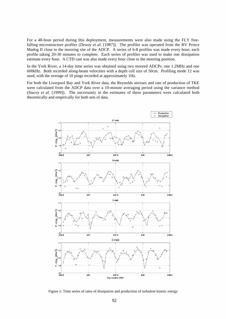
92

For a 48-hour period during this deployment, measurements were also made using the FLY free-falling microstructure profiler (Dewey et al. [1987]). The profiler was operated from the RV PrinceMadog II close to the mooring site of the ADCP. A series of 6-8 profiles was made every hour; eachprofile taking 20-30 minutes to complete. Each series of profiles was used to make one dissipationestimate every hour. A CTD cast was also made every hour close to the mooring position.

In the York River, a 14-day time series was obtained using two moored ADCPs: one 1.2MHz and one600kHz. Both recorded along-beam velocities with a depth cell size of 50cm. Profiling mode 12 wasused, with the average of 10 pings recorded at approximately 1Hz.

For both the Liverpool Bay and York River data, the Reynolds stresses and rate of production of TKEwere calculated from the ADCP data over a 10-minute averaging period using the variance method(Stacey et al. [1999]). The uncertainty in the estimates of these parameters were calculated boththeoretically and empirically for both sets of data.

Figure 1: Time series of rates of dissipation and production of turbulent kinetic energy

93

3. ResultsSome results from the Liverpool Bay observations are shown in figure 1. The results show closetracking of dissipation and production estimates, particularly near the bed. For both P and ε, the datawere averaged temporally over 1 hour and spatially over 1m. Both P and ε show high values (O 10-2

W/m3) extending throughout the water column at times of peak flow on the flood phase of the tidalcycle (day numbers 246.9, 247.4, 247.9). On the ebb the peak values of P and ε are lower; in theupper part of the water column the noise in the production estimates is much more evident.

Further results on the cycle of production from the York River will be used to compare strong andmarginally stratified conditions and to demonstrate the lower noise level resulting from the increasedping rate.

4. Initial ConclusionsProduction and dissipation are closely consistent at 1 hour averages. With the lower noise levelsobtained using mode 12, there arises the possibility of an improved comparison of P and ε which mayreveal the differences between them due to the other terms in the TKE equation.

References:

Dewey, R.K., W.R. Crawford, A.E. Gargett and N.S. Oakey (1987) A microstructure instrument forprofiling oceanic turbulence in coastal bottom boundary layers. J. Atmos. Oceanic. Technol., 4, 288-297

Rippeth, T.P., N. Fisher and J.H. Simpson (2001) The cycle of turbulent dissipation in the presence oftidal straining. J. Phys. Oceanogr., 31, 2458-2471

Simpson, J.H., J. Brown, J. P. Matthews and G. Allen (1990) Tidal straining, density currents andstirring in the control of estuarine stratification. Estuaries, 13(2), 125-132

Stacey, M.T., S.G. Monismith and J.R. Burau (1999) Measurements of Reynolds stress profiles inunstratified tidal flow. J. Geophys. Res., 104, 10933-10949

��

��

�� !��"### �� $� ��

�� %�� $&�� %�� '�(��)�

�� #�� $�� $� ��

��

�� !��"### �� $� ��

� ��

�� !��"�� ! �� #�� #� �� #� � �� $�� %&'(�� #� �� )� �� )� �� *�� #�� +�� !�� ! �� #�!�� ! �#� � ��

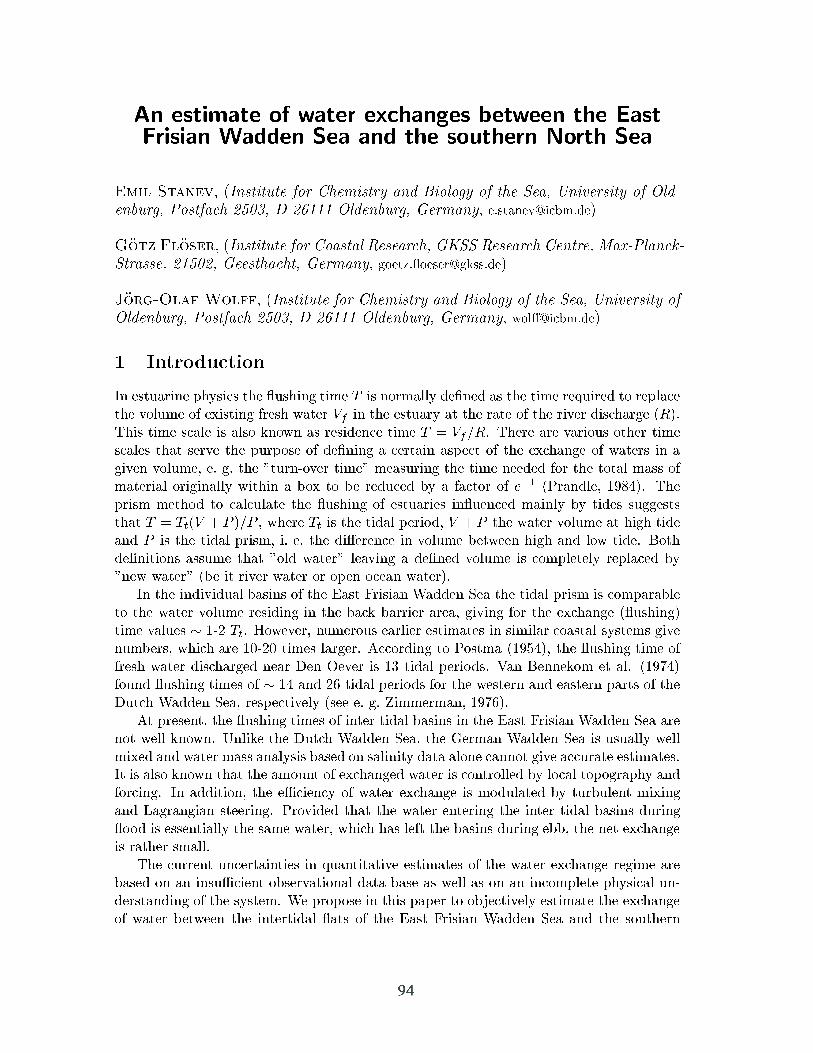
�� #�� ,�� -�� .�� /�� #�� #� � #�� %"0 �� 1�� #�� %2"02 �� 3 �� $�� %&4(� �� 5�� 6�� %7 �� 8�� +�� %&9(�� %( �� 0: �� 5�� .�� /�� ;�� %&9:��

3� �� #�� ,�� -�� .�� /�� <�� 5�� .�� /�� =�� .�� /�� #�� #� �� Æ �� #� ��#�� >�� $�� #�� #�� ## ��

�� #�� Æ �� #�� #�� "�� .� �� #?� �� #�� ,�� -�� .�� /��

@�� /�� *�� #�� "�� " ��

� � ��

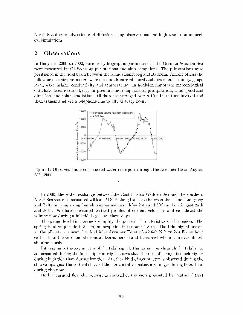
�� 0222 �� 0220 �� =�� .�� /�� #� =A// �� #�� #�� >�� +�� 3�� B �� #�� #�� 3�� %2 �� =A// ��

-�� %B 6#�� 3 �� ,� �� 3��04�� 0222

�

�� 0222 �� #�� ,�� -�� .�� /�� @�� /�� 35C$ �� #�� >�� +�� D�� 0:�� 72�� 3�� 04�� 72�� .� ��

�� B �� 7�( � �� #�� %�' �� 3 �� ,� �� 47 (0�:49 @ 9 0'�097 , �� 5�� +��

�� B �� 3�� #�� B �� E�� ## ��

+�� #� $�� %&'0�

�� F �� #�� "#�� 6�� *�� #� $�� #�� .�� /��

� ��

�� #�� =�� ,�� D�� =,�D� �� 7"5 �� +�� +�� 0220�� #�� #� /�� 0220��

-�� 0B >�� ?� ��

.� �� E�� 022 � �� #�� =�� 1�� 6Æ � �� =�� +�� /�#"�� E�� "� ��#�� #�� "�� #��

�� #�� /�� 0220�� #�� ?� �� >�� :("��

+� �� -�� #�� .�� /�� >�� +�� (�' 7�9 (�' �� %�4 � ��

� ��

�� #�� ,�� -�� @�� /�� *�� "�� +�" ��

�� 35C$ �� B �� #� �#�� *� �� E�� #�� -�� 7� �� #�� /�� >�� -�� 7# �� #�� #�� /�� 0220�� -�� 7 �� *�� #��

-�� 7B �� #�� #� �� #��

�� .� �� 1�� +�� A�� +�� "�� =,�D �� G�� G��H��

��

�� !"��#�� $ %"�& ��

�� '()*'+,� -)+,�

�"�&�� .� �� /� �� !�0� � �� "�� 1�� # �"��*

�� &� 2�1� !32 454(' !6� !"��1�� -(+ 11�� 4554�

7�� .�� .8 ��1&8 �$ �&� %"�& �� 9 ,*''� -)(,�

7�� %�� " 8 �$ �&� �:�� $ -'+�� &� �� $ �&� !"��1��

�&��$� �� ;�� 9 ,5+*,'<� -)=,�

�� !� >� ��*?� �� .� �"�&�� /� �� @�A�� ?� �&� ��"�� &� !��

@�� 9 6"�� 8�� "�� 4554�

B�� @� 0:�� "�&�� $ � �� 8�� &� �� %"�& ��

7�� C9 %��"�� $ ��8 �� "�� $ �:�� -,)*-)-�

-)+<�

98

Waves in inletsPAULO SALLES

(Engineering Institute, National Autonomous University of Mexico, Apdo. Postal 70-472,Coyoacán 04510, México D.F., México, [email protected])

RODOLFO SILVA

(Engineering Institute, National Autonomous University of México, Apdo. Postal 70-472,Coyoacán 04510, México D.F., México, [email protected])

JUAN CARLOS ESPINAL

(Engineering Institute, National Autonomous University of México, Apdo. Postal 70-472,Coyoacán 04510, México D.F., México, [email protected])

1. IntroductionInlet hydrodynamics are complex. They result from the interaction between the fluid motion and thebottom floor, which often has a complicated spatial distribution (channels, bars, deltas, platforms…).The fluid motion is in turn generated both by currents (tidal-induced, wind-driven, wave-generated,river flow...) and by waves, which propagated at frequencies ranging from a few seconds to severalhours or more.

In spite of that, inlet hydrodynamics, and in general inlet stability, are commonly studied withemphasis on the currents (e.g., Bruun, 1978; Salles, 2000). This is reasonable when the inlet is tidedominated, which is the case when the tidal amplitude is large compared with the wave energy at theinlet gorge. In addition, even if considerable wave energy exists in the vicinity of the inlet, many inletshave a well-developed ebb-delta that causes the waves to break before reaching it. However, in caseswere no ebb-delta is present and the tidal amplitude is small, waves can play a major role in sedimenttransport, and in general in inlet morphodynamics.

In order to analyze the effects of waves on inlet dynamics, a series of projects have started, includingfield measurements, mathematical and numerical modeling. This study is the first effort in that sense,and consists of numerical simulations of the hydrodynamics in Laguna de Términos, Mexico, a largecoastal lagoon system, and in particular in Puerto Real, a flood-dominated inlet, to compare thesediment transport capacity with and without waves.

2. Study areaThe Laguna de Términos coastal system is located in the coastal plains of the State of Campeche. Itcommunicates with the Gulf of Mexico through two natural inlets, Carmen and Puerto Real inlets, eastand west of the Carmen barrier island, respectively, and Sabancuy Inlet, a small artificial inlet, 43 kmnortheast from Puerto Real Inlet. The system is composed by a main water body with 3.5 m averagedepth and a surface area of approximately 1,700 km2, and a series of adjacent lagoons, some of whichare the deltas of rivers entering the main lagoon (see

Figure 1), with a total surface area of 800 km2. The flood area, up to the +1.0 m relative to the meansea level, is of 4,000 km2.

The climate is tropical humid and is characterized by three stations, regulated by the rain intensity:little precipitation (March to May), heavy rains (June to October), and intermediate precipitations withstrong northerly winds or Nortes (November to February). The average yearly precipitation is 1,805mm (David et al., 1998), and the yearly evaporation has been estimated to be 1,512 mm, which givean average effective input, considered uniformly distributed over the entire system, of 23 m3.s-1. Theaquatic vegetation is represented by sea grass (Thalassia testudinum, Halodelue wrightii y

99

Syringodium filiforme), and the lagoons are surrounded by mangrove (Rhizophora mangle, Avicenniagerminans, Laguncularia racemosa, y Conocarpus erectus). The predominant winds are moderatewith north-northeast and east-southeast wind speeds lower than 5 m.s-1, except during the Nortesseason, in which frontal passages can have average sustained north-northwest wind speed in excess of12.5 m.s-1 (Mancilla et al., 1980).

010

2030

4050

105

kilo

met

ers

0.0

0.0

0.0

0.0

0.0

0.0

0.0

0.0

0.0

0.0

0.0

0.0

0.0

0.0

1.0

1.0

1.0

1.0

1.0

1.0

1.0

1.0

2.0

2.0

2.0

2.0

2.0

2.0

2.0

2.0

0.0

Dig

ital

Ter

rain

Mo

del

fro

m E

PO

ME

X

X=120,000

X=160,000

X=200,000

Y=

10,0

00

Y=

50,0

00

Y=

90,0

00

Isla

del

Car

men

Est

ero

de S

aban

cuy

Boc

a de

l

Pue

rto

Rea

l

Bo

ca d

el

Car

men

Lag

un

a P

uer

to R

ico

Lag

un

a P

om

Lag

un

a A

tast

a

Bo

ca d

e A

tast

a

Bo

ca C

hic

a

Lag

un

a S

itio

Vie

jo

Lag

un

a d

e P

anla

u Río Candelaria

Río

Mam

ante

l

Lag

un

a d

e T

érm

ino

s

Lag

un

a d

el E

ste

Río Palizada

Río

Ch

um

pán

Gu

lf o

f M

exic

o

Sta

tio

n 1

2

Figure 1. Map of Laguna de Términos, with lines corresponding to +0.0, +1.0 and +2.0 m.

Most of the fresh-water input to the system comes from three rivers (see Figure 1): Palizada river withmonthly-averaged discharges ranging from 115 to 510 m3.s-1 (288 m3.s-1 yearly average), Candelariaand Mamantel rivers, whose discharges occur in the Panlau lagoon, and range monthly from 23 to 197m3.s-1 (72 m3.s-1 yearly average), and Chumpán river with discharges ranging from 0.3 to 50 m3.s-1 (18m3.s-1 yearly average).

100

The tide in the area is mixed-diurnal (Marina, 2001), with the diurnal components being the largest, asshown in Table 1. The average amplitude is 0.424 m, the high high water is 0.923 m and the low lowwater is –0.662 m, with respect to the mean water level (0.000 m). According to measurements of thewater level fluctuations at the inlets and an intermediate point between the inlets (St. 12 in Figure 1),the phase lag of the tide as it propagates inside the lagoon is important, as shown in Table 2. Forinstance, the high O1 tide occurs 1.7 hours later at Carmen Inlet and 5.01 hours later at Station 12. Itcan be seen that the propagation of the tide is from northeast to southwest in that zone of the Gulf ofMexico. Furthermore, the propagation experiences selective dampening inside the lagoon, as a resultof higher friction and energy transfer from one component to another.

Table 1. Main harmonic components

Component M2 S2 N2 K1 O1 P1

H (m) 0.076 0.019 0.021 0.111 0.120 0.036

Phase (º) 78.58 73.63 67.35 315.17 318.93 321.44

Table 2. Phases of the main harmonic components (in degrees and hours:minutes), relative to Puerto Real.

Component M2 S2 N2 K1 O1 P1

Puerto Real 0 0 0 0 0 0

Carmen -33 / 1:08 -8 / 0:16 -39 / 1:22 -36 / 2:24 -24 / 1:43 -27 / 2:01

St. 12 -134 / 4:38 -254 / 8:28 --- -67 / 4:27 -70 / 5:01 -41 / 3:04

The density stratification due to vertical gradients of salinity and/or temperature has been found to beimportant only locally in some areas of the system and during the rainy season, in particular in theriver mouths (Herrera-Silveira et al., 2002), and never at the ocean inlets. Therefore, this stratificationas not been taken into account in this study, which focuses on the inlet hydrodynamics.

3. Numerical modelNumerical simulations of the tidal dynamics in the system, using RMA-2V (Donnell et al., 1997), avertically integrated finite-element model that solves the non-linear momentum and continuityequations, complemented with COPLA-2DH (COPLA-RD, 1998), a wave parabolic model for thewave propagation under the presence of currents, were performed in order to estimate the flowcharacteristics at the inlet. Finally, the bedload and suspended load sediment transport at differentlocations was computed by means of a combined wave-current bottom boundary layer flow model(e.g., USACE, 2001). The environmental parameter considered for this studies were: waves, wind,tides, river discharge, Coriolis effects, bathymetry, and grain size (d50= 0.2 mm), for two differentscenarios: (1) spring tide and 1 m waves, and (2) storm surge and 3 m waves.

4. Preliminary Results and DiscussionPreliminary results of sediment transport (considering maximum river discharges, and no direct windeffects) with and without waves have been computed as an example for six points distributed acrossthe Puerto Real Inlet gorge (Figure 2), as show in Figure 3.. It can be seen that the ratio of the wave-current total sediment transport to the pure current value is significantly large: 77 (on average) for thestorm surge case (with 3 m waves) and 29 for the spring tide case (with 1 m waves).

101

Figure 2. Points for sediment transport computations

Although a similar analysis of the effects ofwaves on sediment transport can be doneanalytically, this example shows theimportance of considering waves whenstudying the morphological evolution ofcoastal features as inlets. In Laguna deTérminos, especially in the flood dominantPuerto Real Inlet, the wave effects onsediment transport are considerable. Thelarge sediment transport capacity obtainedwhen considering waves in this inlet isconsistent with the observed morphologicevolution.

Figure 3. Cross-sectional averaged ratio of total sediment transport with and without waves (crosses) withforcing: (a) 1 m storm surge superimposed to spring tide and 3 m waves, and (b) spring tide with 1 m waves

Acknowledgments: This work was partially supported by the UNAM-PAPIIT project number IN106101.

References:

Bruun, P. (1978). Stability of Tidal Inlets, Theory and Engineering, Elsevier.

COPLA-RD (1998). Modelo integral de propagación de oleaje y corrientes en playa., Manual deUsuario, versión 1.0. Universidad de Cantabria.

David, L. T. and B. Kjerfve (1998). “Tides and Currents in a Two-Inlet Coastal Lagoon: Laguna deTérminos, México.” Continental Shelf Research 18(10): 1057-1079.

Donnell, B. P., J. I. Finnie, J. V. Letter, W. H. McAnally, L. C. Roig and W. A. Thomas (1997). User'sGuide to RMA2 WES Version 4.3. US Army Corps of Engineers - Waterways Experiment StationHydraulics Laboratory. pp.

Herrera-Silveira, J. A., R. Silva Casarín, P. Salles Afonso de Almeida, G. J. Villalobos Zapata, I.Medina Gómez, J. C. Espinal González, A. Zaldivar Jiménez, J. Trejo Peña, M. González Jáuregui, A.Cú Escamilla and J. Ramírez Ramírez (2002). Análisis de la Calidad Ambiental Usando ndicadoresHidrobiológicos y Modelo Hidrodinámico Actualizado de Laguna de Términos. CINVESTAV-IPN,Mérida, EPOMEX, Instituto de Ingeniería-UNAM. 187 pp.

102

Mancilla, M. and M. Vargas (1980). “Los primeros estudios sobre la circulación y el flujo neto deagua a través de la laguna de Términos, Campeche, México.” An. Instituto de Ciencias del Mar yLimología, UNAM 7(2): 1-12.

Marina, S. d. (2001). Tablas de Mareas, Golfo de México y Mar Caribe. Dirección general deOceanografía Naval.

Salles, P. (2000). Hydrodynamic Controls on Multiple Tidal Inlet Persistence. MIT/WHOI JointProgram in Applied Ocean Sciences and Engineering, Massachusetts Institute of Technology / WoodsHole Oceanographic Institution: 272 pp.

USACE (2001). Coastal Engineering Manual. Washington D.C.

103

Seasonal variability in the near-surface salinity field of thenorthern and eastern Gulf of MexicoWILLIAM W. SCHROEDER

(Marine Science Program, The University of Alabama, Dauphin Island Sea Lab, 101Bienville Blvd., Dauphin Is., AL, USA, 36528, [email protected])

STEVEN L. MOREY

(Center for Ocean – Atmospheric Prediction Studies, The Florida State University,Tallahassee, FL, USA, 32306-2840, [email protected])

JAMES J. O’BRIEN


1. IntroductionHistoric hydrographic data show a seasonal pattern in the near-surface salinity field of the northernand eastern Gulf of Mexico (GoM). Numerical simulations of the GoM using the Navy Coastal OceanModel (NCOM) predict a similar signal. In this study, the roles of mesoscale eddy activity and theannual cycle of both river discharge and wind forcing are examined in connection with the seasonalpattern of the salinity field. It is demonstrated that the annual cycle of the wind-driven transport ofbuoyant, low salinity water near the Mississippi River Delta greatly influences the interseasonal spatialpattern of the near-surface salinity field in the northern and eastern GoM. Model results show that lowsalinity waters produced by the Mississippi River plume are directed westward onto the broadLouisiana -Texas shelf in the fall and winter and remain insulated from deeper Gulf waters as they aretrapped along the coast. On the other hand, the river plume spreads over deeper slope waters east ofthe delta in the spring and summer forming a low salinity surface layer that can then interact with theoffshore circulation. Mesoscale eddies associated with the Loop Current often entrain these lowersalinity waters and transport them great distances. This mechanism for redistributing the freshwaterdischarged by large rivers in the northern GoM is described from the model results and compared withobservational data sets.

2. The Gulf of Mexico EnvironmentThe circulation in the GoM is dominated by the energetic Loop Current and its associated eddies. TheLoop Current (LC) enters the basin through the Yucatan Channel and exits through the Florida Straitsto the east, forming an anticyclonically flowing current. The LC penetrates northward andintermittently pinches off large anticyclones with irregular periods from 3 and 17 months (see Sturgesand Leben [2000]). These anticyclones drift westward where they decay against the westerncontinental margin. Associated with the LC and the large anticyclones are a wealth of smallercyclonic and anticyclonic eddies interacting in a seemingly chaotic manner. All of these features havevertical scales from several hundred to 1000 m and thus remain offshore of the continental shelf break.

Wind patterns over the northern GoM are typified by light southeasterly winds during the summer,with frequent cold fronts shifting the mean winds to northeasterly and northerly during the fall andwinter. The influence of the seasonality of the winds on the GoM circulation is small compared to theenergetic LC-induced circulation, but can be important near the coast.

Coastal regions of the GoM exhibit large variability in salinity, which in turn has a large influence onthe coastal ocean stratification. Filaments and lenses of low salinity water have been observedthroughout the Gulf. The source of this low salinity water is freshwater discharged by large rivers tothe Gulf, primarily the Mississippi River. The Mississippi River has an annual mean discharge of over

104

13,000 m3/s (as measured by the U. S. Geological Survey gauging station 7374000) with theneighboring Atchafalaya River discharging at about one-half the rate. The monthly climatology of theMississippi River discharge has a maximum in April of over 22,000 m3/s and a minimum inSeptember of just over 6,300 m3/s. A unique feature of the Mississippi River is that the dischargelocations are located at the end of a delta extending to very near the edge of the continental shelf.Thus, if the river plume is directed toward the east, it will extend over deep water, whereas it will flowover the wide Louisiana-Texas (LATEX) shelf should it be directed westward.

Occasional plumes of low salinity water have been observed along the eastern edge of the meanposition of the LC, just offshore of the West Florida Shelf (see Gilbes, et al. [1996]), and have beenshown to be likely linked to discharge from the Mississippi River. Monthly climatology of nearsurface (10 m) salinity from the 1998 World Ocean Atlas (WOA98) (see Conkright, et al. [1998])shows a seasonal signal along this path, which would be consistent with more frequent occurrences ofthese plumes during the summer months. The purpose of this work is to investigate, using a numericalmodel of the GoM together with observational data, this seasonal variability of upper ocean salinity inthe northern and eastern GoM in connection with these low salinity plumes. The roles of seasonalvariability of river discharge and seasonally varying wind stress over the northern GoM on the fate ofthe freshwater discharged by the Mississippi River are examined in connection with the LC-inducedoffshore circulation.

3. The ModelThe NCOM is a three-dimensional primitive equation hydrostatic ocean model developed at the NavyResearch Laboratory (see Martin [2000]). The model’s hybrid sigma (terrain following) and z(geopotential) level vertical coordinate is useful for simulating upper ocean processes in domainsencompassing both deep ocean basins and very shallow shelves. The NCOM is set up to simulate theentire GoM and Caribbean north of Honduras (15° 30' N) to 80° 36' W with 1/20° between likevariables on the C-grid, 20 sigma levels above 100 m and 20 z-levels below 100 m to a maximumdepth of 4000 m. The model is forced by discharge from 30 rivers, transport through the openboundary (with monthly climatology temperature and salinity) yielding a mean transport through theYucatan Strait of approximately 30 Sv, and monthly climatology surface heat and momentum flux. Asurface salinity flux has the effect of uniformly evaporating an amount of water at a rate equal to thesum of the annual average discharge rates of the 30 rivers.

4. Results and DiscussionMonthly climatology salinity averaged over 1°x1° boxes at 10 m from both the WOA98 and NCOMsimulations with steady river discharge and monthly varying river discharge show similar seasonalsignals along the eastern edge of the mean position of the LC (Figure 1). The salinity minimumoccurs in the summer during which the model salinity field has a tongue-like spatial pattern with lowervalues to the north near the Mississippi River. The amplitude of the seasonal signal decreases withdistance from the freshwater source. The similar results from the two model experiments suggest thatseasonal variability of river discharge does not play an important role in determining the variability ofthe surface layer salinity far from the river mouth.

105

Figure 1: Left: NCOM mean August surface salinity shown with the mean position of the LC. Right: Monthlyclimatology surface salinity from 1°x1° boxes (shown north to south) from WOA98 (10 m) (gray), NCOM withsteady river discharge (dashed), and NCOM with monthly river discharge (black).

Continuous underway observations of surface salinity made during the Northeastern Gulf of MexicoPhysical Oceanography Program: Chemical Oceanography and Hydrography Study (NEGOM) cruises(Minerals Management Service sponsored Texas A & M University Study) are consistent with thesalinity fields predicted by the NCOM simulations. Spreading of low salinity water from theMississippi River eastward is evident over the deep DeSoto Canyon during the summer, with no sucheastward spreading evident during the winter (Figure 2).

Ekman transport of the buoyant low salinity water near the mouth of the Mississippi River isresponsible for the seasonal eastward and westward spreading of the plume. During the winter, whenthe wind is from the north, the plume turns westward and is coastally trapped, insulated from the deepocean by the wide LATEX shelf. In the summer months, the light southerly winds direct the plumeeastward over the deep DeSoto Canyon. Jets formed by interacting eddy pairs found throughout theGoM can entrain buoyant low salinity water which has spread offshore over the deep water in whichthese eddies exist. That is, water discharged by the Mississippi River can interact with the eddies nearthe DeSoto Canyon when the plume spreads in this direction primarily in the summer. These jetsoften form a pathway to the LC, which transports this low salinity water far from its origin in thenorthern GoM (See Schroeder, et al. [1987]).

The mechanism responsible for the seasonal signal of upper ocean salinity found along the easternedge of the LC has two ingredients. The first is the spreading of the Mississippi river plume over thedeep DeSoto Canyon to the east in the summer and the wide LATEX shelf to the west in the winter,directed by the seasonally varying wind stress. Entrainment of water by jets between interacting deepwater eddies forms the second ingredient, to which there is no seasonal component.

Acknowledgments: The authors thank Drs. Paul Martin, Alan Wallcraft, and others at the Navy ResearchLaboratory for their development of and assistance with the Navy Coastal Ocean Model. The Texas A&MOceanography Department provided the plots for Figure 2. Simulations were performed on the IBM SPs atFlorida State University and the Naval Oceanographic Office. Computer time was provided by the DoD HighPerformance Computing Modernization Office. This project was sponsored by funding provided by the DoDDistributed Marine Environment Forecast System, by the Office of Naval Research Secretary of the Navy grantawarded to Dr. James J. O'Brien, and by a NASA Office of Earth Science grant to the COAPS authors.

106

Figure 2: Surface salinity from continuous underway measurements from the NEGOM cruises Nov. 13-24, 1998(top), and July 25 – Aug. 6, 1998 (right). (Provided by the Department of Oceanography, Texas A & MUniversity)

References:

Conkright, M., S. Levitus, T. O'Brien, T. Boyer, J. Antonov, and C. Stephens, World Ocean Atlas1998 CD-ROM Data Set Documentation.. Tech. Rep. 15, NODC Internal Report, Silver Spring, MD,16 pp., 1998.

Gilbes, F., C. Tomas, J. J. Walsh, and F. E. Muller-Karger, An episodic chlorophyll plume on theWest Florida Shelf, Continental Shelf Research, 16, 1201-1224, 1996.

Martin, P., A description of the Navy Coastal Ocean Model Version 1.0. NRL Report NRL/FR/7322-009962, Naval Research Laboratory, Stennis Space Center, MS, 39 pp., 2000.

Schroeder, W. W., S. P. Dinnel, W. J. Wiseman., Jr., and W. J. Merrell, Jr., Circulation patternsinferred from the movement of detached buoys in the eastern Gulf of Mexico, Continental ShelfResearch, 7, 883-894, 1987.

Sturges, W., and R. Leben, Frequency of ring separations from the Loop Current in the Gulf ofMexico: A revised estimate, Journal of Physical Oceanography, 30, 1814-1819, 2000.

107

S

K E E

K

Subtidal variability of flow around a capeARNOLDO VALLE-LEVINSON AND CATHY BROWN

(Center for Coastal Physical Oceanography, OEAS Department, Old Dominion University,Norfolk, Virginia, USA, [email protected], [email protected])

1. IntroductionStudies of flows around capes have documented the generation of secondary circulations resultingfrom curvature effects [e.g. Geyer, 1993]. These circulations develop at intratidal time scales andconsist of surface flow away from the cape and bottom flow toward the cape. On average, tidal flowsinteracting with capes or headlands tend to produce a pair of counter-rotating eddies that have beenportrayed in the horizontal plane [e.g. Signell and Harris, 2000]. Little is known about the verticalstructure of the mean flow around a cape and on its subtidal variability. Our objective is then toillustrate the subtidal variability of the vertical structure of the flow at a site off a cape and todocument the dynamics associated with the flow. This objective is addressed with current velocityprofiles obtained for almost five months. The velocity profiles were combined with time series ofnear-surface and near bottom salinity, near surface and near-bottom temperature, sea level, and windvelocity .

2. ObservationsData were collected off Cape Henry (36° 55.768’N, 75° 59.955’W), the southern cape at the entranceto Chesapeake Bay(Fig.1), from January 20to June 9, 2000 over adepth of 6 m. Thevelocity profiles weremeasured with a 614.4kHz RD InstrumentsAcoustic Doppler CurrentProfiler (ADCP) equippedwith pressure sensor. Atotal of 45 pings wereaveraged over 15 minutesat vertical bins of 0.5 mand with the first bin at~0.8 m from the bottom.Salinity and temperaturevalues were measuredwith SeaBird’s SBE-37recorders. Hourly windvelocity and sea level datawere obtained fromNOAA s ta t ions a tChesapeake Bay BridgeTunne l (#8638863) ,Kiptopeke (#8632200) andS o l o m o n s I s l a n d(#8577330)(E, K, Srespectively on Fig. 1).

Figure 1. Map of the study area showing the lower Chesapeake Bay in thecontext of the eastern United States. The mooring location is indicated bythe arrow pointing at a small white circle at the entrance to the bay. Thedark dotted line indicates the Chesapeake Bay Bridge Tunnel (CBBT). Thesymbol E denotes the location of the wind station at CBBT.

108

ESK

S - EK - E

3. Data ProcessingFlow measurements were purged from values for which the “error velocity” exceeded 5 cm/s or the“percent good” fell below 80%. The purged velocity values were rotated 37° counterclockwise tomaximize the inflow/outflow direction. Positive values represented flows out of the estuary for theprincipal-axis component, and toward Fishermans Island for the transverse component. All time serieswere filtered with a Lanczos low-passed filter of 34-hr half-power. Therefore, this study concentrateson the subtidal variability of flow profiles. The ADCP record was also decomposed into EmpiricalOrthogonal Functions (EOFs) to explore the different modes of variability and to support the findingson the site dynamics.

4. Results

Three predominant directionscharacter ized wind forc ing:northwesterly, northeasterly andsouthwesterly (Fig. 2a). The strongestwind pulses had a northerlycomponent and produced increases innon-tidal sea-level (Fig. 2b) and set-upin the lower bay as indicated bynegative slopes (Fig. 2c). Also,southwesterly winds caused decreasesin non-tidal sea level (Fig. 2b) and sealevel set-downs (positive slopes, Fig.2c). Salinity records (not shown)illustrated weakly stratified conditionsthat suggested limited influence ofbaroclinic pressure gradients to thedynamics of the study area.Figure 2. Wind forcing and sea level response during observation

period.

Figure 3. Low-passed variabilityof a) wind andamplitude of tidalcurrent; b) prin-cipal axis of flow(positive is out-flow); c) verticalshear of the flowprincipal axis (Η100 s-1; dark con-tour delineates re-gions of negativeshears); and d)anomalies fromthe mean for thesubtidal flow.

109

Along-channel mean flow

Across-channel mean flow

Non-tidal currents flowed out of the estuary practically during the entire period of observation (Fig.3b). Most of the subtidal variability of the flow was produced by the wind. Net outflow was strongestwhen winds were from the northwest and southwest because of the orientation of the estuary. Therewere only a few instances when the subtidal flow was directed into the estuary associated withnortheasterly winds. However, not every northeasterly wind caused net inflow. The vertical shearsassociated with the non-tidal flows were mostly positive (Fig. 3c). Strongest positive shearsdeveloped with southwesterly and northwesterly winds. Negative shears (subsurface outflow strongerthan surface outflow) appeared preferentially with northeasterly winds. Anomalies of the non-tidalflow, relative to the overall mean at each depth, were strongly positive with northwesterly winds andstrongly negative with northeasterly winds (Fig. 3d). This response indicated that the non-tidal flowsat the study site were most sensitive to northerly winds.

A fortnightly modulation of tidal forcing, as depicted in Figure 3a, appeared associated with strongersubtidal flows during spring tides than during neaptides (Fig. 4a). These subtidal flows, again, were inthe same direction throughout the water column. Theunidirectional flows contrast with the typical density-induced exchange flows that strengthen during neaptides in several estuaries and that have beenextensively documented. In the transverse direction,the non-tidal flows were very weak and wereindependent of tidal forcing (Fig. 4b). Centrifugalaccelerations should have been stronger at springtides and would have produced surface flow awayfrom the cape and bottom flow toward the cape. Thiswas not the case in our observations (Fig. 4b), whichindicated that non-linear advection was relativelyweak. On the other hand, the enhancement ofunidirectional principal-axis outflows during springtides at our study site (Fig. 4a) is consistent with tidalrectification mechanisms that most likely arise frombottom friction. Therefore, bottom friction shouldplay a role in the dynamics of the subtidal variability,in contrast to advective accelerations andbaroclinicity, as explored next.

The relationship among wind forcing, sea levelslopes and bottom friction that is implied by theobservations in Figures 3 and 4 is investigated

through the principal-axis component of the subtidal, depth-averaged momentum balance in whichadvective acelerations are neglected:

Hxgvftu bxsxρρρρ

ττττττττηηηη −−−−++++∂∂∂∂∂∂∂∂−−−−====−−−−∂∂∂∂

∂∂∂∂ (1)

where the x axis is positive seaward; <v> and <u> are the transverse and principal axis components ofthe subtidal flow, respectively; f is the Coriolis parameter (8.8_10-5 s-1 for 37° N); and g, H, _, _, _sx,and _bx are the acceleration due to gravity (9.8 m/s2), water column depth (6 m), density of the water(1020 kg/m3), sea surface elevation, surface stress and bottom stress, respectively. The surfacestresses are calculated as in Large and Pond (1981) with a rotated wind velocity (37°counterclockwise). Bottom stresses are estimated as _bx = _Cb ub |ub | using a non-dimensional bottomdrag coefficient Cb of 0.0025 and the near-bottom (bin closest to the bottom) flow ub.

Every term in the momentum balance (1) is calculated and presented in Figure 5. The shaded regionof Figure 5 represents the barotropic pressure gradient associated with the sea level slope betweenmiddle and lower bay. Negative (onshore) winds cause negative sea level slopes, i.e., water piling up

Figure 4. Mean flow as a function of tidal range.

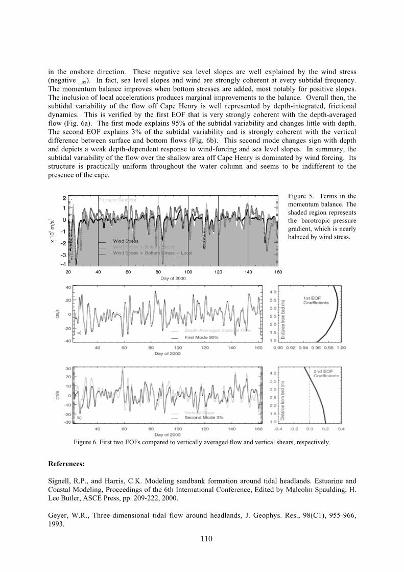
110

in the onshore direction. These negative sea level slopes are well explained by the wind stress(negative _sx). In fact, sea level slopes and wind are strongly coherent at every subtidal frequency.The momentum balance improves when bottom stresses are added, most notably for positive slopes.The inclusion of local accelerations produces marginal improvements to the balance. Overall then, thesubtidal variability of the flow off Cape Henry is well represented by depth-integrated, frictionaldynamics. This is verified by the first EOF that is very strongly coherent with the depth-averagedflow (Fig. 6a). The first mode explains 95% of the subtidal variability and changes little with depth.The second EOF explains 3% of the subtidal variability and is strongly coherent with the verticaldifference between surface and bottom flows (Fig. 6b). This second mode changes sign with depthand depicts a weak depth-dependent response to wind-forcing and sea level slopes. In summary, thesubtidal variability of the flow over the shallow area off Cape Henry is dominated by wind forcing. Itsstructure is practically uniform throughout the water column and seems to be indifferent to thepresence of the cape.

Figure 5. Terms in themomentum balance. Theshaded region representsthe barotropic pressuregradient, which is nearlybalnced by wind stress.

Figure 6. First two EOFs compared to vertically averaged flow and vertical shears, respectively.

References:

Signell, R.P., and Harris, C.K. Modeling sandbank formation around tidal headlands. Estuarine andCoastal Modeling, Proceedings of the 6th International Conference, Edited by Malcolm Spaulding, H.Lee Butler, ASCE Press, pp. 209-222, 2000.

Geyer, W.R., Three-dimensional tidal flow around headlands, J. Geophys. Res., 98(C1), 955-966,1993.

111

Mapping the mixing hot spots in a stagnant fjord basinLARS ARNEBORG

(Department of Oceanography, Göteborg University, Box 460, SE-405 30 Göteborg, Sweden,[email protected])

CAROL JANZEN

(Scool of Ocean Sciences, University of Wales, Bangor, Menai Brige, Anglesey, LL59 5EY,UK, [email protected])

BENGT LILJEBLADH

(Department of Oceanography, Göteborg University, Box 460, SE-405 30 Göteborg, Sweden,[email protected])

TOM P. RIPPETH


JOHN H. SIMPSON


1. IntroductionThe aims with the present study are to i) map the spatial distribution of vertical diffusion in the deepbasin of Gullmar Fjord, and to ii) compare the basin average vertical diffusion obtained frommicrostructure shear probes with that obtained from moored conductivity/temperature (CT) loggers.

Vertical diffusion of heat and salt in the stagnant waters of deep fjord basins is important for oxygenconditions in the basins. The main effect of the vertical diffusion is that it reduces the density, whichenables dense and oxygen rich waters outside the fjord to penetrate to the bottom of the fjord, andreplace the old and oxygen depleted waters (e.g. Aure and Stigebrandt [1990]). Much is known aboutthe bulk effects of tides on the vertical diffusion in fjord basins (e.g. Stigebrandt [2002]), but verylittle is still known about the processes that lead to the turbulence and diffusion. There are turbulencemodels, e.g. the k-ε model, that can describe the diffusion in wind-driven surface- and tidal bottom-boundary layers. These fail, however, in deep basins, where the wind-driven shear is absent, andwhere the tidal velocities are so small that the tidal boundary layer mixing becomes insignificant.Recent experiments in the Brazil basin (Ledwell et al. [2000]) show that i) vertical diffusion is muchenhanced above rough topography relative to above smooth topography, and that ii) the enhanceddiffusion is probably caused by breaking internal waves that are generated by tidal currents flowingover the rough topography. Experiments in lakes (Goudsmit et al. [1997]) indicate that the verticaldiffusion is mainly related to internal seiches, and is concentrated to thin boundary layers at thesloping bottoms. Experiments in fjords with tracers (Stigebrandt [1979]) and microstructure shearprobes (Inall and Rippeth [2002]) show that the vertical diffusion in the interior of fjord basins isgenerally not large enough to explain the basin averaged vertical diffusion. No experiments have,however, shown exactly where the dissipation takes place. Is it concentrated to the waters above roughtopography, as in the abyssal ocean, or is it restricted to thin bottom boundary layers, as in lakes?These questions motivated an intensive study in Gullmar Fjord, some results of which are presentedhere.

Gullmar Fjord located on the Swedish west coast (Fig. 1) is a 28 km long, and 1-2 km wide sill fjord,with sill depth about 43 m and maximum depth about 120 m. Gullmar Fjord is characterised by weaktides (<0.2 m amplitude), weak fresh-water runoff (≈25 m3s-1), short residence times above sill level (1- 2 weeks), and yearly renewals of the otherwise stagnant basin water below 50�60 m depth. Arneborg

112

Figure 1: Sketch of Gullmar fjord, showing the location of the 5 stations D1, G1, G2, G3, and D2, wheredissipation measurements were performed. Moorings with ADCPs (and CTs) were deployed at stations (G1),G2, and (G3).

and Liljebladh [2001] investigated the basin average vertical diffusion and related it to the dynamicsin the fjord based on time series from moored ADCPs and CT loggers. They found that the magnitudeand time-variation of the work against buoyancy forces by vertical diffusion in the deep basin can beexplained by three equally important energy sources. These are i) internal waves of tidal frequency,generated by interaction of the barotropic tides with the sill, ii) internal waves generated by an externalseiche, and iii) the internal seiches in the fjord. They did, however, not perform turbulencemeasurements in the fjord, and could therefore only speculate about the spatial distribution of thediffusion, and the detailed processes leading from the barotropic tides, the barotropic seiche, andinternal seiches down to turbulence and mixing.

2. The ExperimentDuring three days in the beginning of August 2001, two microstructure profilers onboard two researchvessels were used in an intensive effort to map the spatial and temporal variations of vertical mixing inthe deep stagnant basin of Gullmar Fjord. One profiler, the MSS profiler (Prandke et al. [2000]) was

113

used to obtain a continuous time series of turbulent kinetic energy dissipation at station G2 (see Fig. 1)near the deepest part of the fjord. The measurements were performed as bursts of 4 profiles. Theinterval between bursts was 1-2 hours. During the same period the FLY profiler (Dewey et al. [1987])was used to obtain 6 sections through the fjord, with stations at D1, G1, G2, G3, and D2, see Fig. 1.Bursts of 6 profiles were performed at each station visit. The profiles were taken while steaming withapproximately 1 knot, and one burst took approximately 20 min, which means that one burst wasdistributed over the distance of 0.5 to 1 km. During one month, including the 3-day period, mooringswith ADCPs and CT loggers were deployed at station G1, G2, and G3. In addition one ADCP mooringwas deployed in the main entrance and one CT mooring was deployed outside the fjord.

3. ResultsThe intensive 3-day period was characterised by very variable wind conditions, which forced seichingmotions in the deep basin with period close to 1 day. The superposition of the internal seiche andinternal semi-diurnal tides caused vertical oscillations at station G3 with amplitudes larger than 10 m,and horizontal current speeds with amplitudes of about 0.1 ms-1 in the deep waters. Based on thedensity decrease rates obtained from the mooring data the horizontally averaged vertical diffusioncoefficient is found to be in the order of 10-4 m2s-1 in the deepest parts of the fjord, decreasing to 10-5

at 50 m depth. Assuming a constant flux Richardson number, one can determine the dissipation,corresponding to these diffusion coefficients. With a flux Richardson number in the range 0.1-0.2, onegets horizontal average dissipation rates in the order 1-2⋅10-8 W/kg below 60 m depth. Figure 2 shows

Figure 2: Left panel: Bin averages of dissipation rates in 5 m bins, based on all FLY microstructure profiles ateach station. The darkest shaded boxes show the 95% confidence intervals for the average values, estimatedwith a bootstrapping method. Also shown is the depth of the fjord as function of distance from the entrance.Right panel: Buoyancy frequency squared based on an average of all density profiles obtained with the MSSprobe at station G2.

114

the distribution of dissipation in the fjord, as obtained from averages of all FLY profiles at eachstation. At the inner stations the dissipation levels below 60 m range from 2⋅10-9 Wkg-1 at station G1 to4⋅10-9 Wkg-1 at station D1, with some enhancement closest to the bottom caused by boundary layerturbulence. This shows that the dissipation levels in the inner parts of the fjord are up to a factor of 10too small to explain the basin average vertical diffusion. At the outer stations, G3 and D2, however,the dissipation levels below 60 m increase to 3-5⋅10-8 Wkg-1 at station G3, and 10-7 Wkg-1 at D2. Aweighted average of the dissipation levels gives a horizontally averaged dissipation in the order of 1-2⋅10-8 Wkg-1, i.e. enough to explain the horizontally averaged vertical diffusion obtained from themooring data. About 90 % of the vertical diffusion through the 60 m level takes place in the1/3 of thebasin area closest to the sill. The enhanced dissipation rates at station G3 are not limited to a boundarylayer closest to the bottom, but are distributed relatively uniformly over the water column below 50 m.What then causes the enhanced dissipation levels close to the sill? The ADCP at station G3 showsclearly enhanced shear below 60 m relative to the stations G2 and G1. The shears at G3 that arecalculated from 4-hour averaged velocities, low-pass filtered in the vertical direction, passing verticalwave lengths larger than 10 m, are not large enough to cause Richardson numbers below 1. It is,however, clear that a superposition of the high-frequency and high-wavenumber internal wave fieldupon the filtered field, will result in a higher probability for critical Richardson numbers andturbulence at G3 than at the inner stations with less background shear.

Acknowledgments: The present work was supported by EU through the OAERRE project EVK3-CT99-00002.

References:

Arneborg, L, and B. Liljebladh. The internal seiches in Gullmar Fjord. Part II: Contribution to basinwater mixing. J. Phys. Oceanogr., 31, 2567 - 2574. 2001

Aure, J. and A. Stigebrandt. Quantitative estimates of eutrophication effects on fjords of fish farming.Aquaculture, 90, 135-156. 1990.

Dewey, R.K., W.E. Crawford, A.E. Gargett, and N.S. Oakey. A microstructure instrument forprofiling oceanic turbulence in coastal bottom boundary layers. J. Atmosph. Ocean. Tech., 4, 288-297.1987.

Goudsmit, G.H., F. Peeters, M. Gloor, and A. Wüest. Boundary versus internal diapycnal mixing instratified waters. J. Geophys. Res. 102, 27903-27914.

Inall, M.E., and T.P. Rippeth. Dissipation of tidal energy and associated mixing in a wide fjord.Submitted to J. Env. Fluid Mech. 2002.

Ledwell, J.R., E.T. Montgomery, K.L. Polzin, L.C. St. Laurent, R.W. Schmitt & J.M. Toole. Evidencefor enhanced mixing over rough topography in the abyssal ocean. Nature, 403, 179-182. 2000.

Prandke, H., K. Holtsch, and A. Stips, MITEC technology development: Themicrostructure/turbulence measuring system MSS, Tech. Rep. EUR 19733 EN, European Commission,Joint Research Centre, Ispra, Italy, 2000.

Stigebrandt, A. Observational evidence for vertical diffusion driven by internal waves of tidal origin inthe Oslofjord. J. Phys. Oceanogr. 9, 435-441.

Stigebrandt, A. Vertical mixing and circulation in fjord basins. Submitted to Surveys in Geophysics.2002.

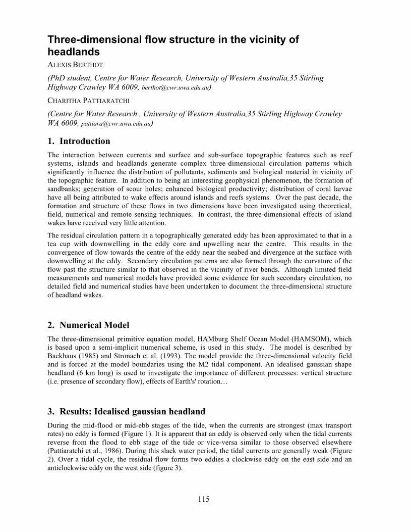
115

Three-dimensional flow structure in the vicinity ofheadlandsALEXIS BERTHOT

(PhD student, Centre for Water Research, University of Western Australia,35 StirlingHighway Crawley WA 6009, [email protected])

CHARITHA PATTIARATCHI

(Centre for Water Research , University of Western Australia,35 Stirling Highway CrawleyWA 6009, [email protected])

1. IntroductionThe interaction between currents and surface and sub-surface topographic features such as reefsystems, islands and headlands generate complex three-dimensional circulation patterns whichsignificantly influence the distribution of pollutants, sediments and biological material in vicinity ofthe topographic feature. In addition to being an interesting geophysical phenomenon, the formation ofsandbanks; generation of scour holes; enhanced biological productivity; distribution of coral larvaehave all being attributed to wake effects around islands and reefs systems. Over the past decade, theformation and structure of these flows in two dimensions have been investigated using theoretical,field, numerical and remote sensing techniques. In contrast, the three-dimensional effects of islandwakes have received very little attention.

The residual circulation pattern in a topographically generated eddy has been approximated to that in atea cup with downwelling in the eddy core and upwelling near the centre. This results in theconvergence of flow towards the centre of the eddy near the seabed and divergence at the surface withdownwelling at the eddy. Secondary circulation patterns are also formed through the curvature of theflow past the structure similar to that observed in the vicinity of river bends. Although limited fieldmeasurements and numerical models have provided some evidence for such secondary circulation, nodetailed field and numerical studies have been undertaken to document the three-dimensional structureof headland wakes.

2. Numerical ModelThe three-dimensional primitive equation model, HAMburg Shelf Ocean Model (HAMSOM), whichis based upon a semi-implicit numerical scheme, is used in this study. The model is described byBackhaus (1985) and Stronach et al. (1993). The model provide the three-dimensional velocity fieldand is forced at the model boundaries using the M2 tidal component. An idealised gaussian shapeheadland (6 km long) is used to investigate the importance of different processes: vertical structure(i.e. presence of secondary flow), effects of Earth's' rotation�

3. Results: Idealised gaussian headlandDuring the mid-flood or mid-ebb stages of the tide, when the currents are strongest (max transportrates) no eddy is formed (Figure 1). It is apparent that an eddy is observed only when the tidal currentsreverse from the flood to ebb stage of the tide or vice-versa similar to those observed elsewhere(Pattiaratchi et al., 1986). During this slack water period, the tidal currents are generally weak (Figure2). Over a tidal cycle, the residual flow forms two eddies a clockwise eddy on the east side and ananticlockwise eddy on the west side (figure 3).

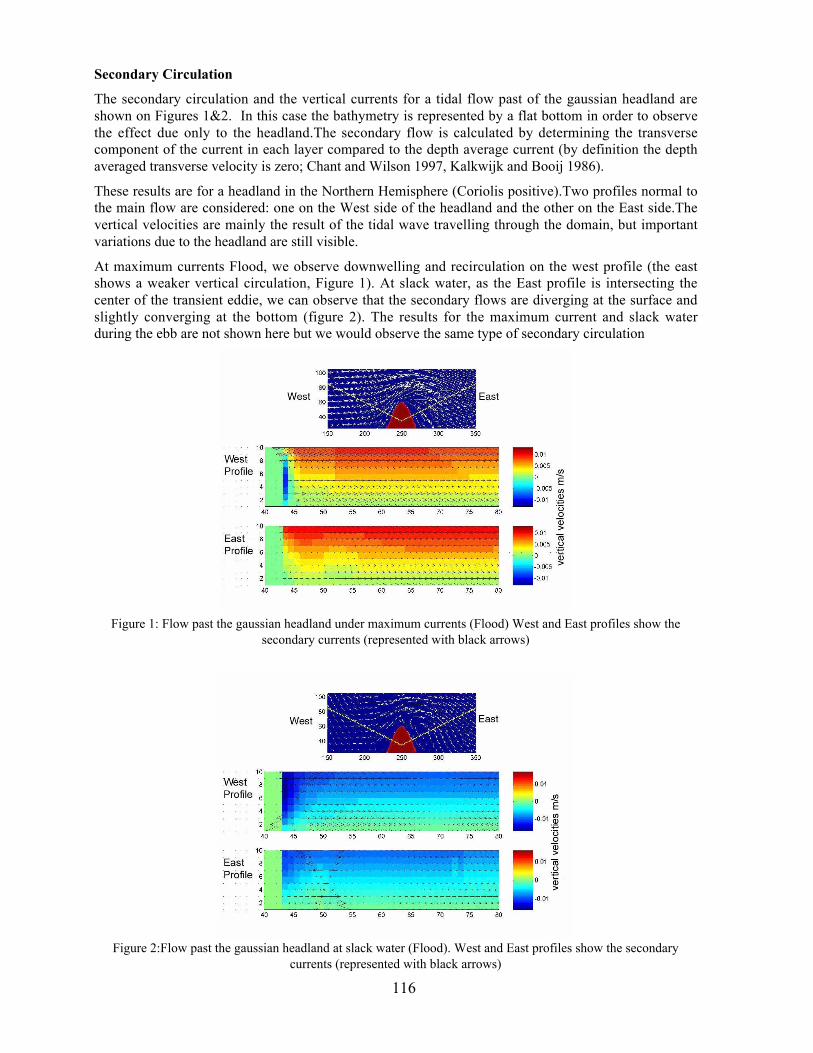
116

Secondary Circulation

The secondary circulation and the vertical currents for a tidal flow past of the gaussian headland areshown on Figures 1&2. In this case the bathymetry is represented by a flat bottom in order to observethe effect due only to the headland.The secondary flow is calculated by determining the transversecomponent of the current in each layer compared to the depth average current (by definition the depthaveraged transverse velocity is zero; Chant and Wilson 1997, Kalkwijk and Booij 1986).

These results are for a headland in the Northern Hemisphere (Coriolis positive).Two profiles normal tothe main flow are considered: one on the West side of the headland and the other on the East side.Thevertical velocities are mainly the result of the tidal wave travelling through the domain, but importantvariations due to the headland are still visible.

At maximum currents Flood, we observe downwelling and recirculation on the west profile (the eastshows a weaker vertical circulation, Figure 1). At slack water, as the East profile is intersecting thecenter of the transient eddie, we can observe that the secondary flows are diverging at the surface andslightly converging at the bottom (figure 2). The results for the maximum current and slack waterduring the ebb are not shown here but we would observe the same type of secondary circulation

Figure 1: Flow past the gaussian headland under maximum currents (Flood) West and East profiles show thesecondary currents (represented with black arrows)

Figure 2:Flow past the gaussian headland at slack water (Flood). West and East profiles show the secondarycurrents (represented with black arrows)

117

Figure 3. Residual currents in the vicinity of the gaussian headland.(Figure showing two eddies on either side ofthe headland) .

Effect of the Earth's rotation

Considering the residual currents over one tidal cycle, we observe the formation of two eddies (Figure3): one clockwise on the east side and one anticlockwise on the east side. To investigate the role of theCoriolis force we run the hydrodynamic model for a headland situated in the Northern Hemisphere(Coriolis positive) and for a headland situated in the Southern Hemisphere (Coriolis negative).

The residual secondary flows in the bottom layer are converging toward the center of the eddy on bothclockwise and anticlockwise eddies (Figures 4 & 5). Nevertheless by observing the strengh of thesecondary flow, it appears that the secondary currents are stronger on the anticlockwise eddy for theNorthern hemisphere and in the clockwise eddy for the Southern Hemisphere.

Figure 4. NORTHERN HEMISPHERE Residualbottom currents in the vicinity of the gaussianheadland.[ residual currents are represented with blackarrows and the secondary circulation with yellowarrows ]

Figure showing the convergence of the secondarycirculation toward the tip of the headland and towardthe center of the eddies. The secondary currents arestronger on the west eddy.

Figure 5. SOUTHERN HEMISPHERE Residualbottom currents in the vicinity of the gaussianheadland.[ residual currents are represented with blackarrows and the secondary circulation with yellowarrows ]

Figure showing the convergence of the secondarycirculation toward the tip of the headland and towardthe center of the eddies. The secondary currents arestronger on the east eddy.

118

4. DiscussionResults of the present model enable us to gain further understanding and detailed structure of the 3dimensional hydrodynamic flow around headland.The secondary flows calculations (for theinstantaneous currents and for the residual over a tidal cycle) also enabled us to identify the validity ofthe different theories proposed for the formation of the headland associated linear sandbanks (Pingree1978, Heathershaw and Hammond 1980). Those results will be later compared with the results ofnumerical study and field measurement (using an ADCP and moored instruments) at Cape Levillain,aheadland with an attached sandbar.

Acknowledgements: US Office of Naval Research

References:

Backhaus J. O. 1985. A three dimensional model for the simulation of shelf sea dynamics. DeutscheHydrographische Zeitschrift, 38: 165-187.

Chant, R. J. and R. E. Wilson. 1997 Secondary circulation in a highly stratified estuary. Journal ofGeophysical Research, vol 102, No. C10, p 23,207-23,215

Heathershaw A.D. and Hammond F.D.C. 1980. Secondary circulation near sand banks in coastalembayments. Dt Hydrogr. Z., 33, 135-151.

Kalkwijk, J. P. T. and R. Booij 1986. Adaptation of secondary flow in nearly horizontal flow. Journalof Hydraulic Research 24., (1): 19-37.

Pattiaratchi C. B., Hammond T. M. and Collins M. B. 1986. Mapping of tidal currents in the vicinityof an offshore sandbank from remotely-sensed data. Int. J. of Remote Sensing, 7: 1015-1029.

Pingree R. D. 1978. The formation of the Shambles and other banks by tidal stirring of the seas.Journal of the Marine Biological Association, UK, 58, 211-226.

Stronach J. A., Backhaus J. O. and Murty T. S. 1993. An Update on the Numerical Simulation ofOceanographic Processes in the Waters between Vancouver Island and the Mainland: The GF8 Model.Ocean. Mar. Biol. Annual Review, 31: 1-86.

��

��

� ��

�� !"##$%&� �� ' � �� (��)�� '�� * �� +��'��

, '�� -�� .�� '�� /�� 0�' ��

�� 1� �� ' �� 1� ��

�� !$223%&�� 4�� )

�� 1� �* �� )��

� � ��

�� +��'�� ' 5�� *�� (��)+��'�� 6�'�� $& ��' (�� 3)$"�"### ��$&� �� $7)$3� "### �8$2##&� /�� 2)$$� "### �8"9##&�6��"#)":� "##$ ��:& �� 6�� $;� "##" ��;&� �� $� �8$2#� ��:& �� $" �� "; �� $� �8"9##��;&� 8��'�� ,��& �� & �� ' �� ' �8$2## ��&� +��)�� <� ,�� 5�� &�

� ��

�� '�� 5�� $ � �� ; � ��' �� =�� ' �� =�� $# ��>� ?��'�

$$2

6�'�� $@ (��

'��A '�� 3;B �� '�� " � �� 5��

�� '�� '�� 5�� ' � � ��*�� 6�� $� �8"9##� ��;&� � ��)=�� 5� ��

�� !$22$% � �� )�� $� �8$2##� ��:& �� '� � �� !$22"% �� C�� '�5�� *�� <(� �� C�� ' �� 5�� 0�� 5��<(� �� '�� '� �� !$223%&�

� ��

��' ��$� �8$2## �� ; �� 5�� 6�'�� "&� �� D)-& �� + /)�& �� '�� & �� 6�'�� " �� 5�� 5��'�� $"�9"& �'�� ' �� !$22"%� �� '�<(� �� 0�� $# ��> �� : �� 8$2## � �� + ��&� ��$; ��> �� + ��' ��$� �� 5� �� $ �� : ��

$"#

−76.2−76−75.8−75.6−75.4−75.236.5

37

37.5

38

129 130 131

−50

0

50

100

DEL1

129 130 131

−100

0

100

−76.2 −76 −75.8−75.6−75.436.5

37

37.5

38

Latit

ude

260.5 261 261.5−50

0

50

CH1900

Vel

ocity

[cm

/s]

260.5 261 261.5

−50

0

50

Vel

ocity

[cm

/s]

−76.2−76−75.8−75.6−75.4−75.236.5

37

37.5

38

Longitude50.5 51 51.5 52

−100

−50

0

50

100

DEL3

Yearday50.5 51 51.5 52

−100

−50

0

50

100

Yearday

ChesapeakeBay

Track

U measured (dot) U reconstructed ( − )

V measured (dot)V reconstructed ( − )

6�'�� "@ +�� '�� & �� )�� &� �� '�

�� 6�� 8$2## �� 5� �� :�# ��> �� <(� �� -� �� $�� : �� *�� '� � �� 0�� 0�� ' � �� '�� '�� '�� /�� &� ��' ��$� � $; �� ' �� '"; �� !$22$%� � �� 5� � �� '�� ' �� $# ��> �� D)- �� $7 ��> �� /)�� ' �� 1� � �� )- �� ' �� 0�� 3#B �� D)- �� /)� �� $; ��> �� +� �� <(� �� 7 ��>� �� '�� 2 ��> �� $; ��> �� + �� ''�� ' �� $: �� ' �� 8"9## �� + �� 9 ��>� (�� "; ��> �� D)- �� ; ��> �� /)� �� '�� 2;B �� D)- �� 9#B � �� /)��6�� $: ��> �� ; ��> �� D)- �� /)� ��

$"$

�'�� 77B � �� D)- �� 9#B � �� /)� �� ' �� "9 �� ' �� 8$2##

�� '� �� '�� '�� 5�� 5�� ''�� '�

�� ' �� '�� ' �� 5�� ' �� =�� !$22"%� 8� �� <(� �� 4�� 5�� Æ�� '�5�� )�� 5�� E�� ' � �� 5�� '�� ) �� =�� ' �� =�� $22F& � �� .� �� ' � �� 5�� 0�� (G�� "###&��

�� H�� <�� <� I�� )�� 5��

�� 7F2)733� $22"�

�� (�� J�<� �� D0�� )�� )�� 5�� ' � ��)��

�� !��" � 329:)32;F� $22F�

I��.� �� (� �� 8�� 8�� /�� #�� $�� %�� &�� $39")$3;2� "##$�

I �.�� J�(�(�� C� �� H�8� �� <�� 1� �� 0�' �� /�� '�� $$ $$&� $:72)$:2;� $22$�

(�� ' ��)�� ( )*

+$'( $�,)-( *,�.(� �� 7:F)793� "###�

+��)I�� J�(�(� I �.�� E �� 1�� ' �� 1� � � #�� ,�� '�� *�� &� �� <�� "97)";F� $223�

$""

123

Large scour holes induced by coastal currentsMAJID JANDAGHII ALAEE

(Ports and Shipping Organization,751 Enghelab Ave. Tehran 15994, IRAN. jandaghi@ir-

pso.com)

CHARITHA PATTIARATCHI

(Centre for Water Research, University of Western Australia, Nedlands 6009, [email protected])

ALI DASTGHEIB

(Ports and Shipping Organization,751 Enghelab Ave. Tehran 15994, IRAN. a_dastgheib@ir-

pso.com)

1. IntroductionInvestigations on generation of scour holes around breakwaters, causing minor or sever damages tothese expensive marine structures, such as the review by Oumeraci (1994 a and b) have shown thatmore basic knowledge on scouring around breakwaters is required. In a 2-dimensional case, scour infront of an upright breakwater is mainly due to the action of standing waves which causes a steadystreaming pattern in a vertical plane resulting in a alternating scour and deposition patterns in front ofbreakwaters.

In a three-dimensional case, laboratory tests by Sumer and Fredsoe (1997) proposed that the majormechanism behind the scour around the heads of rubble mound breakwaters is the formation of lee-wakes vortices in each half period of waves. According to this mechanism, sediment swept into thesevortices is carried out by these flow structures and eventually deposited away from the head ofbreakwater. Therefore a net scour over a period of waves results in a scour hole in front of abreakwater and adjacent to it.

In addition to the aforementioned mechanism, Fredsoe and Sumer (1997) suggested that the plungingbreakers occurring at the breakwater head may cause scouring. The resulting scour hole is located atthe lee side of the break water head with a size in a similar order of size of the jet induced by plunging.

Bathymetric surveys around breakwaters of Rajaee Port, Bandar Abbas-Iran, reveal that a large hole ispresent in the vicinity of the breakwaters heads. The surveys show that the diameter of the hole is ofseveral hundred meters and its depth varies up to –20 m, while the natural depth in the neighbouringareas is about –12 m. The size and location of the hole changes slightly due to the changes in thedominant hydrodynamic conditions in the region.

Figure 1: Khuran (Clarence) Strait and the location of Rajaee Port

124

Rajaee Port, the second biggest port in Iran, is located in the Khuran (Clarence) Strait possessingberths of 5000 m long and two arms of breakwaters of about 5100m. The port is well protectedagainst the waves with Hs=0.8m while a tidal range of 4.2 m causes a strong tidal current of 1.2 m/saround the breakwaters. Previous studies by the authors reveal that a noticeable secondary circulationinduced by the tidal flow curvature is generated in the vicinity of the breakwaters heads (Alaee andDastgheib 2001; Alaee and Pattiaratchi, 1999). The influence of this secondary circulation on themain flow results in a flow pattern which is capable to generate a scouring mechanism.

Figure 2: Location of the scour hole betweenthe breakwater heads

In present study, the flow pattern in the Clarence Strait and particularly, in the vicinity of Rajaee Porthas been successfully simulated. A set of runs using a 3-D numerical model (HAMSOM) confirmsthe presence of a strong secondary circulation induced by the flow curvature. These results are in verygood agreement with the results of predicting method suggested by Alaee et al (1998). Moreover,according to the most interesting part of results, the model predicts the location and size of the scourhole which are in very good agreement with the field surveys. On this basis, it is recommended thatthe interaction between strong coastal currents and large obstacles, such as breakwaters must beconsidered as a likely cause of scouring.

2. Numerical simulationsIn order to investigate the mechanisms responsible for the generation of the scour hole in front ofRajaee breakwaters, a three-dimensional numerical model (HAMSOM) was employed.

Figure 3: Numerical model domains

125

Due to the relatively high tides in the strait (maximum tidal range of 4.2m) the numerical model wasset up for simulating the velocity structure induced by the tidal flow. For this purpose two modeldomains were selected, as shown in Figure 3.

The numerical results reveals the presence of relatively powerful secondary circulation in front ofRajaee port breakwaters. This secondary circulation which is mainly due to the curvature of thestreamlines is shown in Figure 4: velocity vectors on the surface and the contours of main flowvelocity for a typical hour.

Figure 4: Secondary circulation induced by the tidalflow curvature around Rajaee Breakwaters

The results show that the maximum predicted secondary circulation is about 0.16 m/sec while themaximum main flow is about 1.0 m/sec. These results indicate that the strength of the secondarycirculation is about 15% of the main flow which is in good agreement with the Alaee’s formula forestimate of the strength of secondary circulation induced by the flow curvatures (Alaee et al. 1998).For prediction of the position of scour hole near Rajaee Port a critical mean velocity was chosen due tomedian size of bed grains (d50). Using time averaged mean velocity, contours of main flow and thelocation of maximum secondary circulation the position of scour hole can be estimated as Figure 5.

Figure 5: Observed and numerically predicted scour hole in Rajaee Port

3. ConclusionsRecent studies by the authors indicate that curving coastal currents result in a flow curvature-inducedsecondary circulation. The combination of the main and secondary flow may result in scouring. Inthe case of Rajaee Port, this study reveals that the existing scour hole in front of the rubble mound

126

breakwaters is most likely a product of the new flow structure due the generation of secondarycirculation.

References:

Alaee, M.J. and C. Pattiaratchi (1999). A case study of scouring due to the 3-D structure of flowaround breakwaters. Proc. of the fifth international conference on coastal and port engineering indeveloping countries,Vol 1,pp266-276.

Alaee, M.J., C. Pattiaratchi, and G.Ivey (1998) Dynamincs of Isalnd Wakes, PhD Thesis,Centre forWater Research, University of Western Australia.

Fredsoe, J. and B. M. Sumer (1997). Scour at the round head of a rubble-mound breakwater. CoastalEngineering, 29: 231—262.

Oumeraci, H. (1994a). Review and analysis of vertical breakwater failures — lessons learned. CoastalEngineering, Special Issue on Vertical Breakwaters, 22: 3—29.

Oumeraci, H. (1994b). Scour in front of vertical breakwaters — Review of problems. Proc. Int.Workshop on Wave Bamers in Deep Water, Port and Harbour Research Institute, Yokosuka, Japan,Jan. 10—14 1994: 281—307.

Sumer, B. M. and J. Fredsoe (1997b). Scour at the head of a vertical-wall breakwater. CoastalEngineering. Vol. 29, 201—230.

127

Seasonal changes in the vertical structure of a Scottish sealochFINLO COTTIER, MARK INALL, COLIN GRIFFITHS

(Scottish Association for Marine Science, Dunstaffnage Marine Laboratory, Oban, Argyll,PA34 4AD, Scotland, [email protected])

1. IntroductionFjordic and estuarine sites typically undergo seasonal changes in the vertical structure of the watercolumn. In essence, these changes influence the stability of the water column through the variation inhorizontal fluxes, thermal exchange at the surface and the efficacy of mixing processes. At the surface,buoyancy is added in the form of freshwater run-off and solar heating on scales ranging from diurnalto seasonal. In contrast, the properties of the deep water vary slowly by diffusional processes that maybe modified by enhanced vertical mixing. In some instances a rapid change in the deep water mayoccur under suitable conditions causing dense water inflow or complete convective overturn.

The basic system describing the changes in water column stability in a fjordic environment is welldocumented. In this study we look specifically at aspects of enhanced vertical mixing and theseasonal variation in the strength of an internal wave field. Again, internal waves in fjordic systemsare well described (Stigebrant and Aure, 1989) so we have revisited this phenomenon by analysingsalinity, temperature and current data from a near-continuous 13-month mooring deployment.

NorthChannel

GreatPlateau

50m

50m

50m100m

100m

100m

Figure 1: Location map showing the position of the 15-month ADCP deployment, C1, and the stations occupiedby Inall and Rippeth (2002), C2 and C3.

128

2. Location and Data CollectionOur area of study is the topographically complex Clyde Sea on the Scottish west coast. The mainbasin reaches depths of around 200 m and is separated from the strongly tidal and well-mixed NorthChannel by a broad, shallow sill having a maximum water depth of 40 m. The main basin links toInchmarnock Water, which in turn is fed by Lower Loch Fyne. Further, there is an extensive systemof estuaries connected to the Clyde Sea basin accounting for a substantial annual discharge offreshwater (Edwards et al, 1986).

There is semi-diurnal advection of the dense North Channel water across the sill though itsentrainment into the deep waters of the Clyde Sea is periodic. The combination of a strong densitygradient in the basin and strong barotropic tidal forcing presents suitable conditions for the generationof internal waves at the sill that propagate in the basin.

It has been hypothesised, and to some extent demonstrated, that these internal waves are present andcontribute to the enhancement of vertical mixing in an otherwise stable environment (Inall andRippeth, 2002). However, it is clear that the presence and magnitude of this baroclinic signal isclosely linked to the presence and magnitude of the density gradient. Our hypothesis is thatcontribution to vertical mixing by an internal wave varies seasonally because of the seasonal changesin stratification. Our source of primary data from which to test this hypothesis is a 300kHz RDIADCP moored at a depth of 110m in 150m of water. Additional data obtained from the mooringinclude the temperature field as recorded by an array of 10 miniloggers. Salinity and temperatureprofiles of the water column were recorded approximately every three months during a period of 13months.

3. AnalysisInteraction of a barotropic oscillation with changes in topography will tend to generate linear internaloscillations in the density field when the relevant internal Froude number is not small, but less thanunity. The Clyde Sea is a good example of this, experiencing the interaction of a semi-diurnalbarotropic tide with a broad, relatively shallow sill, and a maximum mode-one internal Froude numberof 0.4. We use both the temperature record and the current data to present observational evidence forthe existence and of the internal wave field in the Clyde Sea and to describe its properties.

Jul Aug Sep Oct Nov Dec Jan Feb Mar Apr May Jun0

0.005

0.01

0.015

0.02

0.025

Figure 2: In addition to spring/neap variations in the daily baroclinic power signal at M2 frequencies (fine line),the signal in a depth bin between 12 to 20 m from the surface passed through a 90 day low-pass filter shows aqualitative decrease through the autumn and winter (bold line). Power at this frequency is restored through thespring and summer.

129

Spectral techniques are then used on the ADCP data to analyse the baroclinic part of the signal. Byfocusing on the principal M2 component we show that the energy contained in the baroclinic tidevaries with depth and varies seasonally.

From the changes in the density field we can link the variation in the baroclinic signal to changes inthe degree of vertical stratification. Using this result an estimate of the seasonal contribution tovertical mixing may be made. Further, by comparing the spectral response of the barotropic and thebaroclinic parts of the spectrum we show explicitly that the point of generation for the baroclinic tideis the sill.

06/24 06/29 07/04 07/09 07/14 07/19 07/24 07/29 08/03 08/08 08/130

0.005

0.01

0.015

0.02

0.025

barotropic

baroclinic

1

1

2

2

3

3 4

4

Figure 3: Power of the M2 frequency in the barotropic (solid line) and baroclinic (broken line) components ofthe current velocity measure at C1. The baroclinic response lags the barotropic by approximately 3 days,corresponding to the difference in propagation speeds between the sill and the mooring site.

As a coda to this study, additional ADCP analysis is directed towards looking at the instrumentresponse to a complete convective overturn event, which occurred in late November. We analyse theADCP record for characteristic signatures of the convective event.

References

Edwards, A., M.S. Baxter, D.J. Ellett, J.H.A. Martin, D.T. Meldrum and C.R. Griffths, Clyde SeaHydrography. Proceedings of the Royal Society of Edinburgh, 90B, 67-83, 1986.

Inall, M.E. and T.P. Rippeth, Dissipation of Tidal Energy and Associated Mixing in a Wide Fjord,Environmental Fluid Mechanic, in press, 2002.

Stigebrandt, A and J. Aure, Vertical mixing in basin waters of fjords. Journal of PhysicalOceanography, 19, 917-926, 1989.

Wind Fields Retrieved from Nautical Radar-ImageSequences

Heiko Dankert, Jochen Horstmann, Wolfgang Koch

and Wolfgang Rosenthal

GKSS Research Center, Institute for Coastal Research, Department of CoupledModelling Systems, D-21502 Geesthacht, Germany, [email protected]

1 Introduction

An algorithm is presented for retrieving wind vectors from nautical radar-image sequencesand its application. Thereby data sets from different locations in the North Sea and BalticSea have been analyzed. The image sequences were recorded by the wave monitoringsystem (WaMoS), which has been developed at GKSS Research Center [1], [2].

The frictional force of the local wind field generates the small-scale roughness of the seasurface. This small-scale roughness raises the radar backscatter and therewith the varianceof the mean radar cross section (RCS). The small scattering elements are oriented in thewind direction. Therefore, the RCS of the sea surface first of all depends on the windspeed and on the azimuthal angle between the antenna viewing direction and the winddirection. Due to this dependency the wind vector can be deduced from radar images ofthe sea surface.

The algorithm consists of two parts, one for wind direction and another for windspeed retrieval. Wind directions are locally extracted from wind induced streaks, whichare approximately in line with the mean wind direction. The algorithm assumes winddirection as normal to the gradient of the amplitude image, which is approximated by finitedifferences over an appropriate length. The resulting wind direction is taken as normal tothe retrieved local gradients. Wind speeds are derived from the RCS, by parameterizationof its dependency on the wind vector using a Neural Network. The algorithm was testedand validated using data from a radar mounted in the North Sea. The applicability ofnautical radars for wind retrieval is shown for both tower based and ship borne (moving)instruments.

2 Investigated data

All analyzed data sets discussed here were taken by WaMoS, a system that allows todigitize time series of sea clutter images. It utilizes a nautical radar operating at 9.5 GHz(X-band) with horizontal polarization near grazing incidence. An area within a radius ofabout 2 km is covered with a resolution of ≈10 m in range and ≈12 m in azimuth at adistance of about 750 m from the antenna. The instrument is operated on several towersin the North Sea, e.g. on the Norwegian Oil Platform ”Ekofisk” and in the shallow waterarea at the island of Helgoland. Further experimental sites were located in the NorwegianSea in fall 1995, the Odra Lagoon in summer 1997 and the German Bight in spring 1998.

-20

0

-40

-60

RC

S [

dB

]

-80

-180 -90 0 90 180

Antenna Look Direction vs. Wind Direction [deg]

Figure 1: Radar look direction versus range-integrated RCS for different wind speeds cw. For the blackcurve cw ≈ 5.5 ms−1 and the red curve cw ≈ 3.8 ms−1.

3 Wind direction retrieval

There are two methods for wind-direction retrieval from radar image sequences. One isbased on the well known dependency of RCS on radar look direction [3] and the secondon the direction of wind induced streaks visible in radar images [4] (this issue). In Fig. 1the radar-look direction versus RCS is plotted for different wind speeds. In contrast toVV polarized radars and radars operating at moderate incidence angles there is only onepeak at up wind [3]. Therefore the wind direction dependency of the RCS can be used tofind the wind direction. However, it is not always possible to retrieve the entire azimuth,which is the case for radars based at the coast.

The second method is based on wind-induced streaks, which are visible in radar images(see Fig. 2) and are aligned in wind direction. These streaks have a typical spacing of 200to 500 m and may be caused by features such as local turbulences, streaks from foamor surfractants that are aligned with the surface wind. Wind induced streaks were alsovisible in synthetic aperture radar imagery at similar and larger scales and are used toretrieve the wind direction [4], [5] (this issue). In this paper the wind-induced streaks areassumed to be approximately in line with the mean wind direction

The wind-induced streaks have periods much longer then surface waves. By integrat-ing a radar-image sequence over time (typically 32 images representing 1 min of data),signatures with higher variability in time (like surface waves) are averaged out. Onlystatic patterns like the breakwaters and quasi-static signatures, with frequencies muchlower then the integration time, remain visible. The wind-induced streaks are definedto be oriented normal to the local gradients derived from smoothed amplitude images.The average image is therefore further iteratively smoothed and subsampled to obtain aso-called Gaussian pyramid. From level to level the resolution decreases by a factor oftwo; the image size decreases correspondingly to a pixel size of 100 m, 200 m and 400m, representing scales between 200 and 800 m. From these pixels the local directions are

900

1120

680

460

240

(b)(a)

Figure 2: Mean RCS of a radar-image sequence of 64 images taken on the island of Helgoland onNovember, 26th 1999. The wind speed was 18 ms−1 and the measured wind direction 188◦. The retrievedlocal wind direction at the ocean surface are given in (a) by the superimposed blue arrows and the orangedashed lines give the global in situ wind direction at a height of about 90m. For wind-speed retrieval theblue mark covers areas in (b) are not considered for wind-speed retrieval. The polar image is divided intosubareas in range and azimuth. The numbers give the distance from the radar antenna [m].

computed with a 180◦ ambiguity. The 180◦ ambiguity can be removed using the results ofthe first method. In Fig. 2a the resulting mean directions are plotted for one sample scale.It can be seen that they agree well to the wind direction measured at the radar platform.

4 Wind speed retrieval

It is well known that the backscatter of the ocean surface is primarily caused by thesmall-scale surface roughness, which is strongly influenced by the local wind field andtherefore allows the backscatter to be empirically related to wind. Investigation of 2months of radar-image sequences, representing 444 acquisition times show a strong windspeed dependency of the RCS for wind speeds between 5 and 15 ms−1. For wind speedsabove 15 ms−1 there is a large scatter, which cannot be explained so far.

To retrieve the wind speed a NN is used as a multiple nonlinear regression techniqueto parameterize the relationship between the ocean surface wind speed and RCS [6] (thisissue). As a first step, an NN was trained to retrieve the wind speed from the radar-imagesequences. Therefore each sequence is integrated over time to get the mean intensity, whichis correlated with the wind. The mean image as seen in Fig. 2 is divided into subareasof three 200 m-range intervals starting at 680 m and azimuth intervals of 5◦. The meanintensity of each range-azimuth cell together with corresponding antenna-look directionand the in-situ data (wind speed and direction) are the input parameters to the NN. Areaswith shadows due to buildings or static patterns (blue area) were not considered for thetraining of the NN.

0 90 180 270 360Measured wind directions [o]

0

90

180

270

360

Est

imate

d w

ind

dir

ecti

on

s [o

]

corr = 0.93bias = -27.76rms = 35.41

corr = 0.78bias = -12.26rms = 42.31

0 5 10 15in situ wind speed [ms-1]

0

5

10

15

rad

ar

win

d s

peed

[m

s-1]

corr

bias

rms = 1.5

= 0.79

= 0.02

7

(a) (b)

Figure 3: Scatterplots of in-situ wind directions versus radar-derived wind directions (a) and in-situwind speeds versus wind speeds retrieved using the NN (b). For the wind directions, the purple points giveexceptional image sequences, recorded during low-tide. The statistical values in grey are for all considereddata sets and in black only for image sequences without the exceptions.

5 Comparison to in-situ data

The wind vector has exemplary been determined for a data set of 444 image sequences,which were acquired at the island of Helgoland. In Fig. 3a in-situ measurements of winddirections are plotted versus radar retrieved directions. There is a clear dependency be-tween them. The correlation coefficient is 0.78 considering all image sequences. Someexceptions are visible (purple), where the estimated wind direction is about the same andseems to been independent from the measured direction. All of these outliers were re-trieved at low tide and do not represent the directions causes by the wind. They resultfrom the bathymetry, which is imaged by the radar due to the strong tidal currents andthe breaking waves. Omitting these low-tide images the correlation becomes 0.93. Theeffects due to bathymetry can be solved by eliminating the static bathymetry pattern, byaveraging of series of low-tide images and subtracting the mean image from each low-tideimage. This high-pass filter lets only the variable wind signatures pass. Fig 3(b) gives ascatterplot of the in-situ wind speeds versus radar retrieved wind speeds. The radar-windspeeds were retrieved using a NN with input of RCS and wind directions. A correlationof 0.79 and a rms error of 1.57 ms−1 could be achieved.

6 Conclusions and outlook

An algorithm for ocean-wind field retrieval utilizing nautical radar-image sequences hasbeen developed and tested on data sets from different locations. The wind directions areextracted from wind induced streaks. In most cases the wind direction could be retrievedexcept for a few sequences except recorded during low-tide, where bathymetry becomesthe significant imaged pattern in the radar images. Comparison resulted in a correlation

of 0.93. In this paper the wind direction was estimated for local areas to get a field ofwind directions. The wind speed is retrieved from the RCS and wind direction informationusing a NN. Comparison of RCS derived wind speeds to in-situ measurements resulted ina correlation of 0.79 and a rms error of ≈ 1.57 ms−1. As can be seen in Fig. 2 morethen 50 % of the area covered by the radar couldn’t be considered, because of the harborconstructions of the island, shadows due to buildings and the island itself. Further imagesequences recorded during low tide couldn’t be considered as well for wind retrieval. Andfurthermore the coarse-sampled in-situ wind speed data could not give better results here.Overall the results show that it is possible to use the nautical-radar data for the retrievalof wind fields.

Acknowledgments

The authors were supported by the European Commission in the framework of the Euro-pean project MaxWave (project no.: evk: 3-2000-00544). All radar image sequences werekindly made available by the company Oceanwaves.

References

[1] F. Ziemer, “An instrument for the survey of the directionality of the ocean wavefield,” in Proc. of the WMO/IOC Workshop on Oper. Ocean Mon. Using SurfaceBased Radars, Geneva, 1995, vol. 32, pp. 81–87.

[2] K. Hessner J.C. Nieto Borge and K. Reichert, “Estimation of the significant wave heightwith x-band nautical radars,” in Proceedings of the 18th International Conferenceon Offshore Mechanics and Arctic Engineering (OMAE), St. John’s, Newfoundland,Canada, 1999, number OMAE99/OSU-3063.

[3] H. Hatten, J. Seemann, J. Horstmann, and F. Ziemer, “Azimuthal dependence of theradar cross section and the spectral background noise of a nautical radar at grazingincidence,” in Proc. Int. Geosci. Remote Sens. Symp. 1998,, Seattle, USA, 1998.

[4] J. Horstmann, W. Koch, and S. Lehner, “High resolution wind fields retrieved fromSAR in comparison to numerical models,” in Proc. Int. Geosci. Remote Sens. Symp.,Toronto, Canada, 2002.

[5] J. Horstmann, W. Koch, S. Lehner, and R. Tonboe, “Ocean winds from RADARSAT-1ScanSAR,” Can. J. Remote Sens., in press.

[6] J. Horstmann and S. Lehner, “Global ocean wind fields from SAR data using scat-terometer models and Neural Networks,” in Proc. Int. Geosci. Remote Sens. Symp.,Toronto, Canada, 2002.

135

Tidal and subtidal attenuation in the Patos Lagoon accesschannelELISA HELENA L. FERNANDES

(Fundação Universidade Federal do Rio Grande (FURG), Depto. de Física, CP 474, RioGrande-RS, CEP 96201-900, Brazil. [email protected])

ISMAEL MARIÑO-TAPIA

(University of Plymouth, Institute of Marine Studies, Drake Circus, Plymouth, PL4 8AA,United Kingdom, [email protected])

KEITH RICHARD DYER

(University of Plymouth, Institute of Marine Studies, Drake Circus, Plymouth, PL4 8AA,United Kingdom, [email protected])

OSMAR OLINTO MÖLLER

(Fundação Universidade Federal do Rio Grande (FURG), Depto. de Física, CP 474, RioGrande-RS, CEP 96201-900, Brazil, [email protected])

1. INTRODUCTIONProcesses affecting the hydrodynamics of coastal lagoons, including exchanges between the lagoonand the adjacent inner continental shelf, are controlled by tidal and subtidal oscillations. Tidalexchanges are continuous and are predictable as they are periodic. Subtidal processes arise in responseto meteorological forcing over time scales on the order of days. The subtidal forcing can be separatedinto 1) non-local forcing, which includes coastal sea-level changes due to changes in barometricpressure and non-local wind (driven by the Ekman transport acting 90o to the left of the wind); and 2)local forcing, which includes local wind stress (acting on the surface of the water) and freshwaterinflows. Modelling experiments were carried out to assess the attenuation of the tidal and subtidaloscillations in the Patos Lagoon access channel (Figure 1).

2. METHODOLOGYThe energy spectrum of a month long time series of water elevation from January 1992 was calculatedin order to identify the frequency separating the tidal and subtidal oscillations (Figure 2). The diurnal(D), semi-diurnal (SD) and quarter-diurnal (QD) energy peaks can be observed in the spectrum,characterizing the Patos Lagoon mixed tide with diurnal predominance. The diurnal tidal oscillationsare approximately one order of magnitude greater than the semi- and quarter-diurnal peaks, andalthough the energy spectrum suggests subtidal oscillations, spectral peaks cannot be identified.

A high-pass/low-pass filter (Fast Fourier Transformation technique – FFT) was then applied to thetime series of water elevation in order to separate the high frequency time series, representing the tidaloscillations, and the low frequency time series, representing the long period (subtidal) oscillations. Thehigh and low frequency water elevation time series were then used as the ocean boundary condition toforce the TELEMAC model in two independent simulations in order to individually study the behaviorof the tidal and subtidal oscillations in the access channel. The surface boundary condition was a stresscalculated from the components of the wind velocity (prescribed as 7 ms-1 from the NE), and a flowrate of 3000 m3 s-1 was prescribed at the top of the lagoon. Simulations were carried out based on finiteelement mesh of 2631 triangles. Fernandes et al. (2001) and Fernandes et al. (in press) present thecalibration and validation of the TELEMAC model for the Patos Lagoon

136

10-6

10-5

10-4

10-3

10-4

10-3

10-2

10-1

100

D

SD QD

Figure 1 – The Patos Lagoon estuary. Figure 2 – Energy spectrum of the time series of waterelevation – January 1992.

3. RESULTSKjerfve & Knoppers (1991) comment that the single, long and narrow channel that usually connectschoked coastal lagoons to the ocean naturally serves as a hydraulic low-pass filter in reducing oreliminating tidal effects inside the lagoon. Modelling results indicate that the Patos Lagoon is noexception. The entrance channel not only filters the astronomical tides but also attenuates the longperiod oscillations generated offshore, and the tidal and subtidal influence is rapidly reduced as itprogresses landwards. Some oscillations can still be observed 20 km inland, but they disappear at thetop of the estuary (60 km from the mouth). Moller et al. (1996) also point out the attenuation of theseoscillations throughout the channel, although a coefficient describing the tidal and subtidal attenuationwas not calculated.

Ippen & Harleman (1961) developed a method that relates the relative times of high water along theestuary, the tidal amplitudes, and the phase change to a damping coefficient that specifies the changein amplitude with distance along the estuary caused by friction. Such a method would be appropriatefor estimating the tidal attenuation in the Patos Lagoon estuary if a more comprehensive data set wasavailable. We propose another method to estimate the tidal and subtidal attenuation by shifting fromthe time domain into the frequency domain, and applying a cross-spectral analysis (8 Hanningwindows to a time series of 745 points) carried out in pairs between the original time series prescribedat the ocean boundary and the predicted time series of water elevation calculated at selected pointsthroughout the estuary. The cross-spectral analyses result in a co-spectrum (spectral density function),a coherence spectrum and a phase spectrum. The resulting spectral density function provides theattenuation coefficient of the tidal and subtidal signals at different frequencies.

A cross-power spectrum defines the relationship between two variables. If these variables arecompletely independent the co-spectrum is zero, and if they are identical it becomes the ordinarypower spectrum. The derived coherence between the two times series is a measure of how wellcorrelated the two sequences are as a function of frequency, being equal to 1 if one signal is a constanttimes the other (Butt, 1999). The coherence spectrum has a confidence limit, which is the limit belowwhat the coherence values can occur by chance. Therefore, for frequencies at which the coherence isbelow this limit, any co-spectral estimate would be unreliable.

Figure 3 shows the co-spectrum, coherence and phase spectra at different locations along the estuary(Figure 1) when the model is forced with the tidal signal. The prescribed time series and thepredictions at Praticagem (Figure 3A) match very well and reach a coherence level of almost 1, whichis well above the 95% significance level of 0.22, keeping in phase all the time. The co-spectrum atCanal (Figure 3B) indicates a strong reduction of the tidal energy, and although the time series are stillin phase in the frequencies of interest (0.000011 – 0.000045 Hz), the average coherence between them

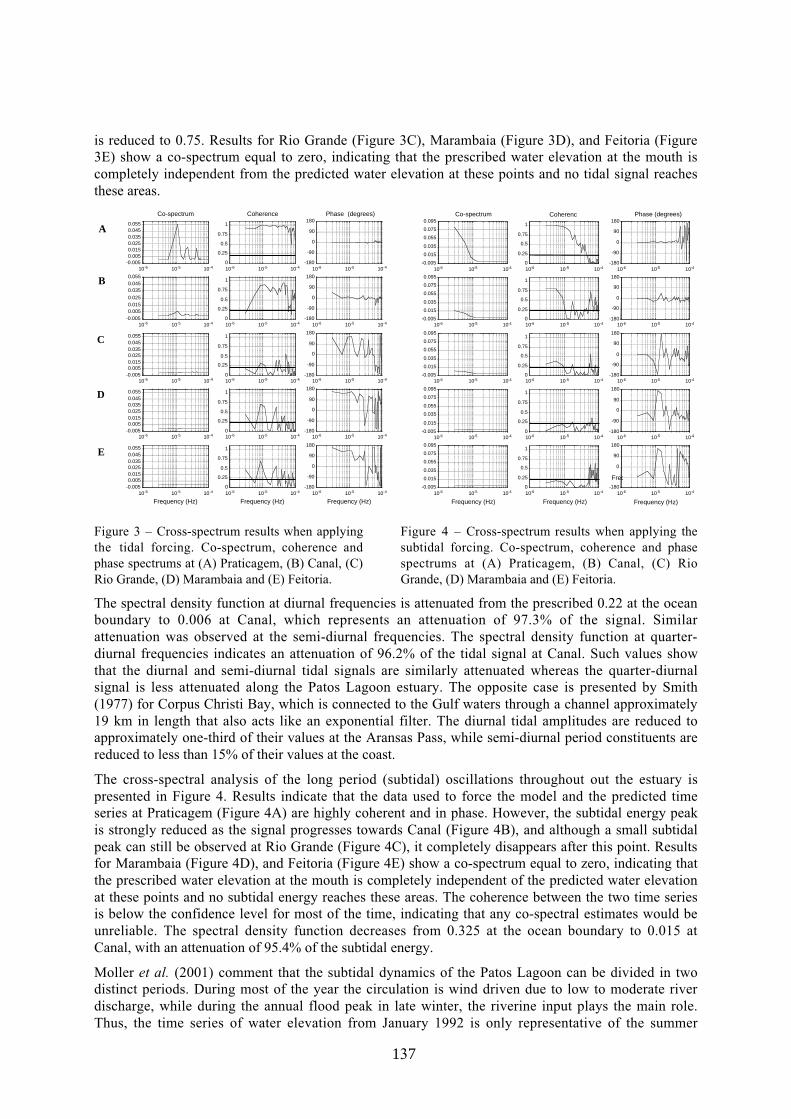
137

is reduced to 0.75. Results for Rio Grande (Figure 3C), Marambaia (Figure 3D), and Feitoria (Figure3E) show a co-spectrum equal to zero, indicating that the prescribed water elevation at the mouth iscompletely independent from the predicted water elevation at these points and no tidal signal reachesthese areas.

Figure 3 – Cross-spectrum results when applyingthe tidal forcing. Co-spectrum, coherence andphase spectrums at (A) Praticagem, (B) Canal, (C)Rio Grande, (D) Marambaia and (E) Feitoria.

Figure 4 – Cross-spectrum results when applying thesubtidal forcing. Co-spectrum, coherence and phasespectrums at (A) Praticagem, (B) Canal, (C) RioGrande, (D) Marambaia and (E) Feitoria.

The spectral density function at diurnal frequencies is attenuated from the prescribed 0.22 at the oceanboundary to 0.006 at Canal, which represents an attenuation of 97.3% of the signal. Similarattenuation was observed at the semi-diurnal frequencies. The spectral density function at quarter-diurnal frequencies indicates an attenuation of 96.2% of the tidal signal at Canal. Such values showthat the diurnal and semi-diurnal tidal signals are similarly attenuated whereas the quarter-diurnalsignal is less attenuated along the Patos Lagoon estuary. The opposite case is presented by Smith(1977) for Corpus Christi Bay, which is connected to the Gulf waters through a channel approximately19 km in length that also acts like an exponential filter. The diurnal tidal amplitudes are reduced toapproximately one-third of their values at the Aransas Pass, while semi-diurnal period constituents arereduced to less than 15% of their values at the coast.

The cross-spectral analysis of the long period (subtidal) oscillations throughout out the estuary ispresented in Figure 4. Results indicate that the data used to force the model and the predicted timeseries at Praticagem (Figure 4A) are highly coherent and in phase. However, the subtidal energy peakis strongly reduced as the signal progresses towards Canal (Figure 4B), and although a small subtidalpeak can still be observed at Rio Grande (Figure 4C), it completely disappears after this point. Resultsfor Marambaia (Figure 4D), and Feitoria (Figure 4E) show a co-spectrum equal to zero, indicating thatthe prescribed water elevation at the mouth is completely independent of the predicted water elevationat these points and no subtidal energy reaches these areas. The coherence between the two time seriesis below the confidence level for most of the time, indicating that any co-spectral estimates would beunreliable. The spectral density function decreases from 0.325 at the ocean boundary to 0.015 atCanal, with an attenuation of 95.4% of the subtidal energy.

Moller et al. (2001) comment that the subtidal dynamics of the Patos Lagoon can be divided in twodistinct periods. During most of the year the circulation is wind driven due to low to moderate riverdischarge, while during the annual flood peak in late winter, the riverine input plays the main role.Thus, the time series of water elevation from January 1992 is only representative of the summer

A

B

C

D

E

10-6 10-5 10-4-0.0050.0050.0150.0250.0350.0450.055

Co-spectrum

10-6 10-5 10-40

0.25

0.5

0.75

1

Coherence

10-6 10-5 10-4-180

-90

0

90

180Phase (degrees)

10-6 10-5 10-4-0.0050.0050.0150.0250.0350.0450.055

10-6 10-5 10-40

0.25

0.5

0.75

1

10-6 10-5 10-4-180

-90

0

90

180

10-6 10-5 10-4-0.0050.0050.0150.0250.0350.0450.055

10-6 10-5 10-40

0.25

0.5

0.75

1

10-6 10-5 10-4-180

-90

0

90

180

10-6 10-5 10-4-0.0050.0050.0150.0250.0350.0450.055

10-6 10-5 10-40

0.25

0.5

0.75

1

10-6 10-5 10-4-180

-90

0

90

180

10-6 10-5 10-4-0.0050.0050.0150.0250.0350.0450.055

Frequency (Hz)10-6 10-5 10-40

0.25

0.5

0.75

1

Frequency (Hz)10-6 10-5 10-4

-180

-90

0

90

180

Frequency (Hz)

10-6 10-5 10-4-0.005

0.015

0.035

0.055

0.075

0.095Co-spectrum

10-6 10-5 10-40

0.25

0.5

0.75

1

Coherenc

10-6 10-5 10-4-180

-90

0

90

180Phase (degrees)

10-6 10-5 10-4-0.005

0.015

0.035

0.055

0.075

0.095

10-6 10-5 10-40

0.25

0.5

0.75

1

10-6 10-5 10-4-180

-90

0

90

180

10-6 10-5 10-4-0.005

0.015

0.035

0.055

0.075

0.095

10-6 10-5 10-40

0.25

0.5

0.75

1

10-6 10-5 10-4-180

-90

0

90

180

10-6 10-5 10-4-0.005

0.015

0.035

0.055

0.075

0.095

10-6 10-5 10-40

0.25

0.5

0.75

1

10-6 10-5 10-4-180

-90

0

90

180

10-6 10-5 10-4-0.005

0.015

0.035

0.055

0.075

0.095

Frequency (Hz)10-6 10-5 10-40

0.25

0.5

0.75

1

Frequency (Hz)10-6 10-5 10-4

-180

Freq

0

90

180

Frequency (Hz)

138

months, when the freshwater discharge is low to moderate and the weather fronts over the region arenot so intense. For such conditions, results presented here indicate that although the subtidal energypropagates further, the tidal and subtidal oscillation have similar magnitudes during the studied period.This picture is expected to change during the winter months, when the area is marked by the passageof much stronger weather fronts and the subtidal oscillations combined with the riverine input fromthe north of the lagoon are expected to overcome the tidal effect.

On the other hand, these experiments are based on simplified conditions and consider a constant windand freshwater discharge at the top of the lagoon. Thus, the long-period oscillations considered hereare limited to the non-local effect, represented by the water elevation at the ocean boundary. Theobserved predominance of subtidal energy will possibly be enhanced when time series of windvelocity and freshwater discharge are available to be included in the calculations.

Further simulations based on improved initial and boundary conditions are currently being carried outin order to investigate the tidal and subtidal attenuation throughout out the seasons in 1992. For now,the presented numerical predictions of the water elevation at different points throughout the estuaryproved to be an alternative method to estimate the attenuation of the tidal and subtidal oscillations inthe channel. Moreover, the calculated attenuation coefficients indicate that the tidal and subtidalamplitude is quite reduced as soon as it leaves the entrance channel. These results agree with theconclusions of Kjerfve and Magill (1989) e Moller et al. (1996).

Acknowledgments: This research was sponsored by the Conselho Nacional deDesenvolvimento Científico e Tecnológico (CNPq), Brazil, contracts 200012/97-5 and540467/01-4. The authors wish to gratefully acknowledge Mr. John Baugh (HR Wallingford)for giving support to the use of TELEMAC-2D.

References

Butt, T. 1999. Sediment transport in the swash-zone of natural beaches. PhD Thesis, Institute ofMarine Studies, University of Plymouth, UK.

Fernandes, E.H.L., Dyer, K.R., and Niencheski, L.F.H. (2001). TELEMAC-2D calibration andapplication to the hydrodynamics of the Patos Lagoon (Brazil), Journal of Coastal Research 34,470:488.

Fernandes, E.H.L., Dyer, K.R., Moller, O. O., and Niencheski, L.F.H. (2001). The Patos Lagoonhydrodynamics during an El Niño event (1998), Continental Shelf Research, in press.

Ippen, A. T. & Harleman, D. R. F. 1961. One-dimensional analysis of salinity intrusion in estuaries.Technical Bulletin No. 5, pp 1-52. Committee on Tidal Hydraulics, CORPS of Engineers, US Army.Kjerfve, B. & Knoppers, B. A. 1991. Tidal chocking in a coastal lagoon. In: Tidal Hydrodynamics. Ed.B. B. Parker. pp. 169-181.

Kjerfve, B. and Magill, K.E. (1989). Geographic and hydrodynamic characteristics of shallow coastallagoons. Marine Geology 88, 187-199.

Moller, O. O., Lorenzzetti, J. A., Stech, J. L. & Mata, M. M. 1996. The Patos Lagoon summertimecirculation and dynamics. Continental Shelf Research 16, 335-351.

Moller, O. O., Castaing, P., Salomon, J. C. & Lazure, P. 2001. The influence of local and non-localforcing effects on the subtidal circulation of Patos Lagoon. Estuaries 24 , 275-289.

Smith, N. P. 1977. Meteorological and tidal exchanges between Corpus Christi Bay and thenorthwestern Gulf of Mexico. Estuarine and Coastal Marine Science 5, 511-520.

139

The effect of variable depths and currents on wavedevelopmentHEINZ GÜNTHER, GERHARD GAYER AND WOLFGANG ROSENTHAL

(Institute for Coastal Research, GKSS Research Center Geesthacht, Max-Planck-Str., D-21502 Geesthacht, Germany, [email protected], [email protected], [email protected])

1. IntroductionIn coastal areas detailed knowledge of the surface wave field is very important for the understandingof hydrodynamic and transport processes. The interaction of waves with the bottom and current is oneof the keys to understand and predict developments in coastal seas.

Substantial progress has been made in the recent years in predicting ocean surface gravity waves. Thethird generation WAM model (Komen et al. [1994]) has demonstrated its excellent performance onglobal and regional scales, which are the deep-water ocean and the shallow shelf sea areas. However,difficulties have been found in the coastal zone. The space and time scales in these areas are normallytoo small to allow the non-linear interactions to control the energy balance. The growth and decay ofwaves is dominated by the input energy from the atmosphere and by enhanced dissipation of waveenergy in the water column and at the sea floor. In particular the dissipation in the water column byturbulent diffusion (Rosenthal [1989]), which is not included in most coastal wave models, has beenidentified as a key process to explain the self-similar spectral shape (Günther and Rosenthal [1995]).

In this paper a brief description of the K-model is presented followed by examples of modelapplications in the tidal area of the Waddensea and around Helgoland to demonstrate the impact ofchanging currents and water depth on the wave development. In these situations the propagationeffects (shoaling and refraction) are balanced by the source functions and especially by the wavedissipation of wave energy.

2. Wave ModelThe K-model is a discreet spectral wave model solving the action density balance equation in wavenumber space (see Schneggenburger, Ch., H. Günther, W. Rosenthal [2000] and Schneggenburger,Ch., H. Günther, W. Rosenthal [1998]). It was developed for small-scale (typical grid resolution from50 m up to a few 100 m) applications with non-stationary currents and water depths. Restricted to theessential physical processes in such environments, the model includes in the source functions theenergy input (modified Snyder source term and Phillips source term), energy dissipation (turbulentdiffusion) and energy dissipation by bottom friction. The source and sink terms are balanced by thepropagation terms, which include refraction and shoaling.

The model is forced by wind fields (at 10 m height, typically every hour) and current and water levelfields (typically every 20 minutes). At land boundaries of the model area free outflow of energy isassumed. At the open sea boundaries wave spectra have to be used. For the following examples thesespectra are taken out of a North Sea model runs with a coarse resolution of 30 km with an inputfrequency of 1 hour.

3. ApplicationsIn the following two applications of the model are discussed. In 3.1 the impact of sea floor changes onwaves and currents in a Waddensea area to the southwest of the Elbe river estuary is investigated. In3.2 a study of the Helgoland area to quantify the impact of variable water depth and/or currents on thewave development and propagation is presented.

140

3.1 Waddensea

To estimate the impact of topographical changes on the wave and current climate in a Waddensea areain the southern North Sea, we examined the results of the spectral wave model and a hydro-dynamicalmodel for different storms and for a 20 days period of moderate weather conditions. Two bathymetrieswere used, one representing the actual condition and a worst case scenario of dredging sand in an areaof approximately 6 km2 increasing the water depth by 2 m from 10 m to 12 m at once.

The model results are compared to find the area of changes and the places where major changes occur.During a north-westerly storm in January 1994 the biggest differences (after dredging – beforedredging) are found to be approximately 20 cm in significant wave height (see figure 1, white areasare land or dry flats. White lines show the 0 and 10 m water depth contours giving an indication of thebathymetry with tidal channels and adjacent flats). The waves at the boundary of the model area had aheight of about 6 m during the peak of the storm.

Figure 1: Differences of significant wave height (after dredging – before dredging) 1994 01 28 18:00.

Only in a spatially limited area at and in the vicinity of the dredging site the wave climate is changednoticeably due to differences in shoaling and energy dissipation. Currents are altered only slightlyafter dredging.

3.2 Helgoland

We investigated the influence of variable current and water level fields on the results of the spectralwave model near the North Sea island Helgoland. This area is characterized by strong water depthgradients (from 50 m – 0 m over a distance of 5 km) especially to the southwest from the island. Twomodel runs were performed, one with unchanged initial bathymetry, another one taking spatial andtemporal water level and current variations into account.

During a storm in October 1998 with wind speeds up to 24 m/s – the wave model calculated asignificant wave height of 5.5 m on a coarse North Sea grid at the nearest grid point to the fine gridarea of interest (50 m resolution) – the waves approached the island from a direction of 290 degrees.

141

Above the slope the wave heights increased to a maximum of 6.5 m due to refraction and shoalingeffects.

Performing the second model run with time series of current and water level variations the shoalingand refraction of waves changed significantly. At high tide shortly after the storm peak a differenceplot of significant wave heights shows especially off the western coast 2 stripes of high differences(see figure 2). In front of the coast positive differences of up to 1.5 m can be observed which can beexplained with greater water depths and reduced energy dissipation. Further to the west negativedifferences of up to 1.5 m show that due to greater water depths the shoaling of waves locally isreduced. The shoaling now takes place in front of the coast, adding there to the high positivedifferences.

Figure 2: Differences of significant wave height (variable depth/currents – constant fields).

4. Conclusions

In small-scale coastal applications the influence of water level and current variations cannot beneglected. The example of the coastal area of the island of Helgoland showed that locally the balanceeffects with shoaling in case of sloping bottom and in the presence of in-stationary water depth andcurrent fields led to high differences in significant wave height fields compared to the scenario withconstant bathymetry. In case of the Waddensea area example changing the bathymetry locally led tomuch smaller differences due to a reduced bottom slope compared to the Helgoland area.

Acknowledgements: Those studies were done in close co-operation with the BAW (Bundesanstalt fürWasserbau), Hamburg.

142

References:

Komen, G. J., L. Cavaleri, M. Donelan, K. Hasselmann, S. Hasselmann, P. A. E. M. Janssen,Dynamics and Modelling of Ocean Waves, Cambridge University Press, Cambridge, UK, ISBN 0 52143291, 560 pages, 1994

Rosenthal, W., Deviation of Phillips a-Parameter from Turbulent Diffusion as a Damping Mechanism,In: Radar Scattering from Modulated Wind Waves, Komen, G. J. and W. A. Oast (eds.), KluwerAcademic Publishers, 1989

Günther, H. and W. Rosenthal, A Wave Model with a Non-linear Dissipation Source Function, inProceedings of the 4th International Workshop on Wave Hindcasting and Forecasting, October 16-20,1995, Banff, Alberta, Canada, pp. 138-148; und GKSS 96/E/62 ISBN 0344-9629.

Schneggenburger, Ch., H. Günther, W. Rosenthal, Spectral wave modelling with non-lineardissipation: validation and applications in a coastal tidal environment, Elsevier Coastal Engineering,41, pp 201 – 235, 2000.

Schneggenburger, Ch., H. Günther, W. Rosenthal, Shallow water wave modeling with nonlineardissipation: application to small scale tidal systems, GKSS 98/E/7, 1998.

143

Sort-period fluctuations of surface circulationsin Sagami Bay induced by the Kuroshio warm waterintrusionHIROFUMI HINATA

(National Institute for Land and Infrastructure Management, 3-1-1 Nagase, Yokosuka2390826,Japan, [email protected])

TETSUO YANAGI

(Research Institute of Applied Mechanics, Kyusyu University, 6-1 Kasuga-Koen, Kasuga8168580, Japan, [email protected])

MASASHI MIYANO

(Ecoh Company Limited, 2-6-4 Kitaueno, Taito-ku, Tokyo 1100014, Japan, [email protected])

TAKASHI ISHIMARU

(Tokyo University of Fisheries, 4-5-7 Konan, Minatoku, Tokyo 1100014, Japan, [email protected])

HIROSHI KAWAMURA

(Center for Atmospheric and Oceanic Studies, Tohoku University, Aramaki, Aobaku, Sendai9808578, Japan, [email protected])

1. IntroductionSagami Bay is located at the southeastern part of Honsyu, Japan and is connected to the Pacific Oceanthrough Oshima West Channel and Oshima East Channel (Fig.1). The Kuroshio flows eastward off

Fig. 1. (a) Schematic diagram of three typical paths of the Kuroshio. (b) Observational region.

Sagami Bay with three quasi-steady paths – the nearshore non-large-meander path (nNLM), theoffshore non-large-meander path (oNLM) and the typical large-meander path (tLM) (Kawabe, 1985).It is well known that when the Kuroshio takes the path of tLM, the Kuroshio Warm Water (KWW)

Honsyu

(°C)

Shikoku

North Pacific

Oshima Is.

nNLM

oNLM

tLM

Sagami Bay

35ºN

33ºN

31ºN

133ºE 135ºE 137ºE 139ºE 141ºE

(a)

(km)

0 10 20 30 40 50 60 70 800

10

20

30

40

50

60

70

80

(km)

OshimaIs.

Tokyo Bay

IzuPen.

MiuraPen.

OshimaWest Channel

OshimaEast Channel

Chigasaki

Tateyama

(b)

144

intrudes into the bay through Oshima west cahnnel and cyclonic and anticyclonic circulations areveloped in the central part of the bay and the lee of Oshima Island, respectively (Taira and Teramoto,1986, Kawabe and Yoneno, 1987, Iwata and Matsuyama, 1989). However, characteristics of short-period fluctuations with a period of several days and precise structures of the circulations remainunknown. In this study, the characteristics of short-period fluctuations and precise flow structures ofsurface circulations in Sagami Bay have been investigated by field observation based on HighFrequency Oceanic Surface Radars (HFOSRs).

2. ObservationThe observation site is shown in Fig.1. Two HFOSRs of Frequency Modulated Interrupted ContinuousWave type (FMICW) were set up at Tateyama and Chigasaki during the period from December 7,2001 to March 6, 2002. Radio waves of the radars have a center frequency of 24.515 MHz with asweep bandwidth of 100 KHz, which results in a range resolution of 1.5 km. Regression analysisshows that the HFOSRs radial current velocity is about 0.93 times that from bottom mounted upwardlooking Acoustic Doppler Current Profiler (ADCP). And the standard deviation of residual is6.5 cms-1. Details are described in Yanagi et al. (2002). 25 hr running averaged HFOSRs currentvelocities were analyzed by Empirical Orthogonal Function (EOF) analysis.

3. Results

KWW had been intruded into the bay through Oshima West Channel during the period fromDecember 15, 2000 to January 16, 2001 (Period 1). And during the Period 1, cyclonic and anti-cyclonic circulations were generated in the central part of the bay and lee of Oshima Island,respectively (Fig.2 (a)).

EOF analysis shows that the first two EOF modes (Fig.3) are dominant and together account for 55%of the variance in the dataset. Time dependent amplitude of the first mode fluctuates with a period ofabout 8-10 days and is highly correlated with variations of sea level in and around Sagami Bay.Increase of sea level drives a positive mode1 response and decrease of sea level a negative response.Fig.2 (b)-(d) shows temporal variations of surface current field reconstructed by EOF mode 1-2 plusthe temporal mean field. Velocities and sizes of the circulations change corresponding to the sea levelvariations with a period of about 8-10 days. The sea level changes in Period 1 in and around SagamiBay are mainly due to the short period fluctuations of the Kuroshio Front (Hinata et al., 2002).

Based on mooring observations and satellite infrared images, Kimura and Sugimoto (1993) pointedout that periodic fluctuations of 5-8 days and 10-12 days in the Kuroshio region are caused by thesmall-scale meander of the Kuroshio front with wavelength of about 100km and 200 km, respectively.Sea surface temperature in the Kuroshio region off Sagami Bay on December 15, 2000 is shown inFig.4. Warm water filaments can be seen in the Kuroshio frontal region and they have about 100-150km wavelength. These results suggest that the fluctuations of two circulations in Sagami Bay arecaused by the small-scale meander (warm water filament) of the Kuroshio front with wavelength of100-150 km.

145

(a) (b)

(c) (d)

100 (cms-1)

20km

_ EOF2 __ EOF1 _

20km

Fig. 2. Surface current maps. (a) Temporal mean flow field , (b) 12:00, Dec. 31, 2000, (c) 12:00,Jan. 03, 2001 and (d) 00:00, Jan. 07, 2001. (b) ,(c) and (d) use EOF mode 1-2 plus the mean field.

Fig. 3. Eigenvector plots of EOF1 and EOF2.

(a)

146

Fig. 4. AVHRR sea surface temperature image in the Kuroshio region off Sagami Bay at 19:52on December 15, 2000 (JST). Arrows indicate warm water filament in the Kuroshio frontal

References:

Kawabe, M. : Sea level variations at the Izu Islands and typical stable paths of the Kuroshio. J.Oceanogr. Soc. Japan, 41, 283-294, 1985.

Kawabe, M. and M. Yoneno : Water and flow variations in Sagami Bay under the influence of theKuroshio Path. J. Oceanogr. Soc. Japan, 43, 283-294, 1987.

Kimura, S. and T. Sugimoto: Short-Period fluctuations in meander of the Kuroshio’s path off capeShiono Misaki. J. Geophys. Res., 98, 2407-2418, 1993.

Hinata, H., H. Miyano, T. Yanagi, T. Ishimaru, T. Kasuya, and H. Kawamura: Short-periodfluctuations of surface circulation in Sagami Bay induced by the Kuroshio warm water intrusionthrough Oshima west channel - Relation to small-scale meander of the Kuroshio front -.Oceanography in Japan (in press).

Iwata, S. and M. Matsuyama : Surface circulation in Sagami Bay: the response to variations of theKuroshio axis. J. Oceanogr. Soc. Japan, 45, 310-320, 1989.

Taira, K. and T. Teramoto: Path and volume transport of the Kuroshio current in Sagami Bay and theirrelationship to cold water masses near Izu Peninsula : J. Oceanogr. Soc. Japan, 42, 212-223, 1986.

Yanagi, T., M. Shimizu, M. Nomura, and K. Furukawa : Spring-Neap tidal variations of residual flowin Tokyo Bay, Japan. Proceedings of 10th Physics of Estuaries and Coastal Seas, edited by A.Levinson, 2001.

0 100 200 300 400 500 600

Sagami Bay36°N

34°N

32°N

30°N

134°E 136°E 138°E 140°E

22 2618141062 (°C)

147

A non-hydrostatic numerical model for calculating of free-surface stratified flows in the coastal seaYULIYA KANARSKA, VLADIMIR MADERICH

(Institute of Mathematical Machine and System Problems, Glushkova av. 42, 03187 Kiev,Ukraine, [email protected])

1. IntroductionThe non-hydrostatic effects are important in a wide spectrum of stratified flows in the coastal seas.The examples are the buoyant plumes from submerged outfalls, internal waves of large amplitudegenerated by the tidally driven flows over a steep topography and exchange flows over the sills in thesea straits. In this paper a three-dimensional numerical model for simulation of the free-surfacestratified flows in the coastal sea is presented. The model is a non-hydrostatic extension of free-surfaceprimitive equation POM model with vertical sigma-coordinate (Blumberg and Mellor [1987]). Thepressure field was decomposed on hydrostatic and non-hydrostatic components. The model equationswere integrated with mode splitting technique and four-stage procedure, where the level wasdetermined at first. The hydrostatic, non-hydrostatic components of pressure, velocity and scalar fieldswere calculated at subsequent stages. Unlike the most of non-hydrostatic models 2D depth-integratedmomentum and continuity equations were integrated explicitly at first stage, whereas 3D equationswere solved implicitly at rest stages. This approach is particularly advantageous for the shallowstratified flows and is fully compatible with the POM model.

The model was tested against laboratory experiments check its ability to reproduce local scale non-hydrostatic phenomena in coastal sea. The surface solitary wave interaction with the vertical wall, theformations of solitary «bulges» in thin pycnocline as the result of the collapse of mixed region andwater exchange through strait are considered.

2. Model DescriptionsThe model is based on the 3D Reynolds-averaged Navies-Stokes equations for Boussinesq fluid. Theconcept of eddy viscosity and diffusivity is used with two-equation model of turbulence model todefine turbulent stresses and scalar fluxes. The sigma-coordinate system for the vertical direction isused. The pressure and velocity fields are decomposed on hydrostatic and non-hydrostaticcomponents. The mode splitting technique (Blumberg and Mellor [1987]) for external and internalmodes was applied. The finite-difference solutions of governing equations were derived using four-stage procedure:

1 stage: Free surface level.

The calculation of free surface elevation is performed by explicit method from depth-integratedshallow water equations like the POM model. The initial 2D velocity fields on each external stage isdetermined by direct integrating of general non-hydrostatic 3D velocity fields from previous internalstep.

2 stage: Hydrostatic components of velocity and pressure.

The 3D hydrodynamic equations without non-hydrostatic pressure are solved with internal time stepsemi-implicitly (Casulli and Stelling [1998]) to determine provisional values of velocity. Theadvection, horizontal viscosity and diffusion were discretized explicitly. The obtained three-diagonalsystem is solved by a direct method.

3 stage: Non-hydrostatic components of velocity and pressure.

The non-hydrostatic components of velocity are computed by correcting the provisional velocity fieldwith the gradient of non-hydrostatic pressure to satisfy continuity equation for sum of hydrostatic and

148

non-hydrostatic velocity. The obtained discretized Poisson equation for the non-hydrostatic pressurereduced to the non-symmetric 15 diagonal linear system, part of which arise from the sigma-transformation components. The preconditioned biconjugate gradient method is used for solving thissystem. Once the non-hydrostatic pressure is determined the corresponding components of velocityfields are calculated.

4 stage: Scalar fields.

The scalar fields (temperature and salinity, turbulent quantities) are computed by using semi-implicitnumerical scheme in vertical direction. The obtained three-diagonal system is solved by a directmethod.

3. Numerical Application and discussionImpact of solitary surface wave on vertical wall. Here, results of a computation are compared with thelaboratory experiments on solitary surface wave interaction with a vertical wall in the wave flume withdepth H. As seen in Fig. 1, the model predicted well maximum of elevation η at the wall. The timedependence of wave pressure on undisturbed surface p is shown in Fig. 2. Non-hydrostatic modelreproduced quite well observed in experiments characteristic two-peak profile of pressure withdepression near to the moment of maximum runup that was caused by the vertical acceleration of fluidat the wall.

Propagation of intrusive �bulge� in the pycnocline. The second example concerned with theformation and evolution of large amplitude intrusive �bulge� that was generated by collapse of mixedregion in the thin pycnocline. The results of simulation are compared in Fig. 4 with experiment 302 ofMaderich et al. [2001] that was conducted in the tank 6.7x0.4x0.19 m. The tank was filled with twohomogeneous layer of different salinity. The circular mixed region with diameter 0.19 m collapsed inthe centre of tank. The resulted solitary bulges (compare Fig. 4 and 5) moved with almost constantspeed that exceeded values, predicted by theory of weakly nonlinear long internal waves.

Exchange flows through long straits with sill. Here, the exchange flow through shallow and narrowstrait connected two deep and wide basins filled by water of different density is considered. Thelaboratory experiment 701 (Maderich [2000]) was simulated. The strait is rectangular with lengthL=60.5 cm, maximal depth H=8 cm and constant width A=0.9 cm. The sill with h/H =0,5 is placed inthe centre. The buoyancy difference is g∆ρ/ρ=1.48 cm/c2. This difference was maintained by heatingof left basin and cooling of right one. The exchange in the strait is maximal. The sill together withright end of strait hydraulically control the exchange, whereas only flow in the lower layer is critical atleft end of the strait. The flow is laminar, however, measurements showed broadening of thermoclineat the left side of sill (see. Fig.6). The computations by non-hydrostatic model were carried out withlaminar viscosity and conductivity and resolution 250x8x100. The internal and external time step were0.015 s and 0.001 s. The simulated density distribution also showed difference between thickness ofinterface on both sides of sill (see Fig.7). The detailed investigation of velocity field in Fig.8 showspresences of complicated flow structure at left side of the sill. The supercritical flow slows down in thepoint of internal hydraulic jump that causes countercurrent. It lifts dense water along the left side ofsill and turns finally to left, forming broad interface layer. The broadening of pycnocline downstreamof sill or contraction was frequently observed in the sea straits, however, it was attributed to theturbulent mixing only. The comparison of non-hydrostatic and hydrostatic calculations was carried outwith the same resolution. Fig.9 indicates essential contribution of nonhydrostatic components at theslope and foot of the sill with the difference in velocities about 20%. Non-hydrostatic calculations isstable for high resolution, whereas hydrostatic calculations was unstable for the same internal step andrequires to reduce internal step by one half.

149

/Hη

0.0 0.2 0.4 0.6 0.8a/H

0.4

0.8

1.2

1.6

2.0123

0.2

0.4

0.6

0.8

1.0

ρ

-4 -2 0 2 4t/T

1

2

p/ g

H

Figure 1: Runup on the vertical wall as a functionof soliton height as measured by Maxworthy[1979] (1), Zagriadskaya and Ivanova [1978] (2)and calculated (3).

Figure 2: Time dependence of wave pressure fordimensionless soliton height a/H =0,5 (1) and0.7 (2). Solid line is simulation and dash line isexperiment (Zagriadskaya and Ivanova [1978]).

Figure 4: Computed intrusion visualized with markers.

0 20 40 60 80t(s)

0.0

0.4

0.8

1.2

1.6

L(m

)

12

Figure 3: Intrusion length as a function of timein experiment 302 (Maderich et al. [2001]) (1)and calculated (2).

Figure 5: Dye-visualized intrusion in experiment 302.

Figure 6: Photo of experiment 701 (Maderich [2000])

Figure 7: Computed density distribution for experiment 701.

150

Figure 8: Interface position in experiment 701 (1) and non-hydrostatic velocity field (2).

Figure 9: Module of difference between hydrostatic and non-hydrostatic velocity fields

4. ConclusionsThe non-hydrostatic model for simulating of free-surface stratified flows in the coastal sea has beendeveloped. The numerical algorithm is a non-hydrostatic extension of POM model and fullycompatible with it. Several oceanographically motivated examples of non-hydrostatic currents wereconsidered. They demonstrate the effectiveness of this tool for wide spectrum of coastal sea problems.

Acknowledgments: This study was partially supported by CRDF project �Improved methodology for assessingthe impacts of the Aegean-Black Sea exchange�.

References:

Blumberg, A.F. and Mellor, G.L. A description of a three-dimensional coastal ocean circulationmodel, in N.S. Heaps (ed.), Three-Dimensional Coastal Ocean Circulation Models, Coastal andEstuarine Sciences, vol. 4, AGU, Washington, DC, 1987, pp. 1�16.

Casulli V., Stelling G. S., Numerical simulation of 3D quasi-hydrostatic, free-surface flows.J. Hydr. Eng., 124, 678-686, 1998.

Maderich V. S., Two-layer exchange flows through long straits with sill. Oceanic Fronts and RelatedPhenomena. Konstantin Fedorov Int. Memorial Symp., IOC Workshop Rep. Series, N 159,UNESCO�2000, 326-331, 2000.

Maderich, V., van Heijst, G.J., Brandt, A. Laboratory experiments on intrusive flows and internalwaves in a pycnocline. J. Fluid Mech., 432, 285-311, 2001.

Maxworthy T., Experiments on collisions between solitary waves. J. Fluid. Mech., 76, 177�185,1976.

Zagriadskaya N. N., Ivanova S. V. Action of long waves on the vertical obstacle. Izv. VNIIG, 138, 94-101, 1988.

151

Fortnight shifts of circulation in Ise Bay and its effect onthe hypoxiaAKIHIDE KASAI, SATOMI AKAMINE, TATEKI FUJIWARA

(Graduate school of Agriculture, Kyoto University. Kyoto, 606-8502, Japan,[email protected], [email protected], [email protected])

TAKUMA KIMURA

(4th Regional Coast Guard Headquarters. 2-3-12 Irifune, Minato, Nagoya, 455-8528, Japan)

HIROKATSU YAMADA

(Fisheries Research Division, Mie Prefectural Science and Technology Promotion Centre. 1-6227-4 Shiroko, Suzuka, 510-0243, Japan)

1. IntroductionIse Bay is one of the major ROFIs (regions offreshwater influence) on the Pacific coast ofJapan (Fig. 1). Three large rivers flow into thebay head in the north and the water inside thebay is stratified through the year. In the souththe bay opens to the Pacific Ocean via narrowIrago Strait, in which strong tidal currents mixthe water. Water exchange between Ise Bayand the Pacific Ocean takes place throughIrago Strait.

Recent surveys on Ise Bay have shown that theflow pattern is different from the classicalestuarine circulation; the strait water does notintrude into the lower layer, but intrudes intothe middle layer along the eastern coast of thebay in summer, because the density of thestrait water is equivalent to that in theintermediate layer inside the bay (Takahashi etal., [2000]; Kasai et al., [2002]). This middlelayer intrusion leads the hypoxia of the bottombay water, which is excluded from theexchange circulation (Fujiwara et al., [2002]).However, there are some observations thatshow the bottom layer intrusion of the straitwater, following the classical estuarine circulation theory. These studies indicate the intrusion depthcould change temporally, but its transition process and the mechanism are still unknown. In this study,therefore, we try to clarify 1) time change in the mixing condition at Irago Strait, 2) time change in theintrusion depth of the strait water, and 3) effects of the intrusion depth on the distribution of thehypoxia.

2. ObservationsObservations of temperature, salinity, and dissolved oxygen (DO) concentration were conducted alongthe longitudinal section of Ise Bay. Observational stations are shown in Fig. 1. To elucidate thetransition process of the intrusion depth and succeeding change in the circulation pattern and the DO

Figure 1: Map of study area. Triangles andcircles indicate observation points by KyotoUniversity and Mie Prefectural Science andTechnology Promotion Centre, respectively.

K4

K7

Ise Bay

Irago Strait

35 No

34 30'No

136 30'Eo

137 Eo

0 20 km

152

distribution, the observations were carried out repeatedly three times a month from June 2000 toAugust 2001.

3. Results and discussionFigure 2 shows examples of the vertical profile of density at Irago Strait (Stn. K7). In the spring tide(thick lines), the water below 20 m was mixed well and nearly homogeneous. On the other hand, itwas weakly stratified in the neap tide (thin lines). It is obvious that mixing condition at Irago Straitwas strongly affected by the tidal strength. There is a negative correlation (r2 = 0.61) between the tidalrange and the density difference between 10 m and 55 m depth at the strait (Fig. 3). The stronger thetidal currents are, the more water is mixed.

Figure 2: Vertical profiles of density at IragoStrait in the spring tide (15 June and 14 July) andthe neap tide (11 August and 6 September).

Figure 3: Relationship between tidal range and densitydifference (55m-10m depth) at Irago Strait (St. 7). Thedata shown by a trianlge is the exception because of theunsusual heavy rain.

Vertical distributions of density along the longitudinal section are shown in Fig. 4. In the spring tides,the density deeper than 15 m at Irago Strait was equivalent to that of the middle layer inside the bay. Aprominent bottom front was created at the bay mouth (25-30 km from the bay head). This bottom frontseparated the Irago water from the dense bottom water inside the bay. On the contrary, at the neaptide, the densities deeper than 15 m at Irago Strait and inside the bay were similar to each other. Itappears that the Irago water intruded through the bottom layer during the neap tide. The weaker tidalcurrent insufficiently mixes the strait water as shown in Fig.2, and thus the bottom water inside thebay becomes lighter than that at the bay mouth where the water tends to stratify. This difference indensity at the bay mouth leads the shift of the intrusion depth. The hydrographic condition changed ina short time period, according to the tidal strength.

In order to know the time change in the intrusion depth, we define the intrusion depth, assuming thestrait water intrudes through the layer that has the same density as that of the strait water. First, thedensities at three depths were selected in Irago Strait (Stn. K7): beneath the pycnocline, at the bottom,and their average as the representative densities of the intrusion water. Secondly the top, bottom, and

153

the centre of the intrusion depth inside the bay (Stn. K4) were defined as the depth that was the samedensity as those beneath the pycnocline, at the bottom and their average in Irago

0 10 20 30

Distance (km)

0 10 20 30 0 10 20 30

0 10 20 300 10 20 30

2 4 6

0 10 20 30

Density (sigma-t)

2 Aug. (Spring) 11 Aug. (Neap) 22 Aug. (Spring)

0

10

20

30

0

10

20

30

D.O. (mg/l)

4 6

24

2

6

24

23

2423

2222

23

Distance (km)

0

10

20

30

0

10

20

302 Aug. (Spring) 11 Aug. (Neap) 22 Aug. (Spring)

Figure 4: Vertical distributions of density and dissolved oxygen along the longitudinal section. Darker areasindicate dense water (> 23) in the upper pannels and hypoxic water (< 4 mg l-1) in the lower pannels.

Figure 5: Time change in (a) the intrusion depth and (b) the tidal range. Open and closed circles indicate middlelayer and bottom intrusion, respectively. Error bars in the upper pannel indicate the top and bottom depth of theintrusion layer.

0

10

20

30

40

1-Apr 1-Jun 1-Aug 1-Oct 1-DecDay

Dep

th (

m)

Bottom

(a)

50

100

150

200

250

300

1-Apr 1-Jun 1-Aug 1-Oct 1-DecDay

Tid

a R

ange

(cm

) (b)

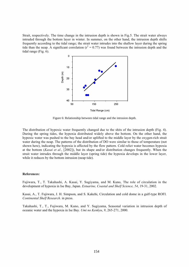
154

Strait, respectively. The time change in the intrusion depth is shown in Fig.5. The strait water alwaysintruded through the bottom layer in winter. In summer, on the other hand, the intrusion depth shiftsfrequently according to the tidal range; the strait water intrudes into the shallow layer during the springtide than the neap. A significant correlation (r2 = 0.77) was found between the intrusion depth and thetidal range (Fig. 6).

Figure 6: Relationship between tidal range and the intrusion depth.

The distribution of hypoxic water frequently changed due to the shits of the intrusion depth (Fig. 4).During the spring tides, the hypoxia distributed widely above the bottom. On the other hand, thehypoxic water was pushed to the bay head and/or uplifted to the middle layer by the oxygen-rich straitwater during the neap. The patterns of the distribution of DO were similar to those of temperature (notshown here), indicating the hypoxia is affected by the flow pattern. Cold relict water becomes hypoxiaat the bottom (Kasai et al., [2002]), but its shape and/or distribution changes frequently. When thestrait water intrudes through the middle layer (spring tide) the hypoxia develops in the lower layer,while it reduces by the bottom intrusion (neap tide).

References:

Fujiwara, T., T. Takahashi, A. Kasai, Y. Sugiyama, and M. Kuno, The role of circulation in thedevelopment of hypoxia in Ise Bay, Japan. Estuarine, Coastal and Shelf Science, 54, 19-31, 2002.

Kasai, A., T. Fujiwara, J. H. Simpson, and S. Kakehi, Circulation and cold dome in a gulf-type ROFI.Continental Shelf Research. in press.

Takahashi, T., T., Fujiwara, M. Kuno, and Y. Sugiyama, Seasonal variation in intrusion depth ofoceanic water and the hypoxia in Ise Bay. Umi no Kenkyu, 9, 265-271, 2000.

155

Numerical Simulation of Wave Transmission at SubmergedBreakwaters compared to Physical ModelingSTEPHAN MAI

(Franzius-Institut for Hydraulic, Waterways and Coastal Engineering, Nienburger Str. 4, D-30167 Hannover, Germany, [email protected])

NINO OHLE


KARL-FRIEDRICH DAEMRICH


CLAUS ZIMMERMANN


1. IntroductionThe design of sea dikes requires knowledge about the wave parameter right in front. Especially thewave propagation along the foreland with structures like summer dikes or submerged breakwaters,determines the wave characteristics at the toe of the dike. Shoaling, refraction, wave breaking, bottomfriction and wave transmission are the predominant processes within this area.

Standard numerical models, like SWAN (see Ris. et al. [1994]), are good tools for the simulation ofthese processes. Nevertheless physical model tests are still needed to calibrate the parameter andvalidate the numerical models.

This paper deals with the wave transmission at summer dikes respectively submerged breakwatersusing the numerical model SWAN as well as laboratory tests in the Large Wave Channel (GWK) ofthe Coastal Research Center (FZK) and in the Wave Basin Marienwerder (WBM) of the Franzius-Institute, both located in Hannover, Germany. The focus is put on the analysis of wave spectrainfluenced by wave transmission.

2. Physical and Numerical Model TestThe model tests in the wave flume GWK with dimensions of 324 m x 5 m x 7 m were carried out atprototype scale. Figure 1 (left) shows the experimental set-up with a summer dike build on a foreland(top) and the wave breaking induced by the summer dike (bottom). The height of the foreland is 1.4 m.The summer dike had a crest height of 1.6 m above the foreland, a crest width of 3 m and a slope of1:7. The parameters of the incoming wave field were varied from 0.6 m to 1.2 m for the significantwave height and from 3.5 s to 8.0 s for the peak wave period at water levels from 3 m to 4.5 m. Thewave propagation was measured at 26 locations along the flume. A detailed description of theexperiments in the GWK is given by Mai et al. (1999a).

The model tests in the wave basin WBM with dimensions of 40 m x 24 m x 1.1 m were carried out ina side channel with a width of 1.7 m. Figure 1 (right) shows the experimental set-up with a submergedrubble mound breakwater with a height of 0.5 m, a crest width of 0.2 m and a slope of 1:2 (top) andthe wave breaking at the breakwater (bottom). The parameters of the incoming wave field were variedfrom 2.5 cm to 17.5 cm for the significant wave height and from 1 to 1.75 s for the peak wave period

156

at water levels of 0.45 m to 0.7 m. Further information on the experiments in the WBM is given byDaemrich et al. (2002).

The data, i.e. time series of water level elevation, collected in both experiments was analyzed in timedomain and also in frequency domain. An example of this analysis is given in figure 2 and figure 3.

In addition to the physical model tests numerical model tests were carried out using the phase–averaged model SWAN (see Ris, 1997) applying the same boundary conditions (bathymetry, waterlevel and wave spectrum). A description of the calibrated model parameter is given by Mai (1999b).An example of the results of the numerical analysis is given in figure 2 and 3.

Figure 1: Experimental set-up in scale in the Large Wave Channel and the Wave Basin Marienwerder at theUniversity of Hannover

3. ResultsAs shown in previous studies (see Mai et al. [1999b]) the characteristic wave parameters (significantwave height and peak wave period) were reproduced correctly by the numerical model. Figure 2exemplifies this for the significant wave height measured in the GWK at a water level of 4 m andincoming waves with a significant wave height of 1 m and a peak period of 8 s. Besides that, theanalysis of the wave spectra at two positions (see figure 2) in the flume also reveals a quite goodagreement for the spectral properties as shown in figure 3. On the left hand side of figure 3 the noninfluenced wave spectrum in front of the submerged breakwater is shown. The right hand side offigure 3 gives a comparable chart for the influenced wave spectrum behind the breakwater.

Due to the transmission at the breakwater the wave spectrum is changed not only with respect to thetotal energy but also with respect to the spectral shape. The loss of total energy results in the decreaseof significant wave height (see figure 2) while the change in the spectral shape results in lower mean

157

wave periods. The change in the wave spectrum is caused by non-linear wave transformation over thesubmerged breakwater resulting in a transfer of energy from the spectral peak to the higher harmonics(see Isobe et al. [1996]). However the spectral peak remains nearly constant (see van der Meer et al.[2000]).

A measure for the energy transfer is the change in the ratio of the energy of the second harmonic (2H)and the energy of the spectral peak (1H). Figure 4 (left) shows the increase of this ratio E2H/E1H

directly at the summer dike for a water level of 4 m and incoming waves with a significant height of 1m and a peak period of 8 s. The energy of the spectral peak with a frequency fp was calculated byintegration of the power spectral density from 0.5 fp to 1.5 fp. The energy of the second harmonic wasset to the integral of the spectral density from 1.5 fp to 2.5 fp.

water level

wavedirection

0 20 40 60 80 100 120 140 160 180 200X [m]

0.60

0.80

1.00

1.20

1.40

sig

. wav

e h

eigh

t H s

[m]

measurementSWAN

0

1

2

3

4

water level z [m

]

poldersummer

dikeforeland

water depth df = 4,0 msig. wave height Hs = 1,0 m peak period Tp = 8,0 s

Position 2Position 1

Figure 2: Change of the significant height of waves propagating over a foreland with summer dike - comparisonof physical modelling (GWK) and numerical modelling (SWAN) (see Mai et al. [1999b]).

0 0.1 0.2 0.3 0.4 0.5frequency [Hz]

0

0.4

0.8

1.2

1.6

pow

er s

pect

ral d

ensi

ty [

m?/H

z]

wave spectrum in front ofa submerged breakwater

numerical model (SWAN)physical model (GWK)

0 0.1 0.2 0.3 0.4 0.5

frequency [Hz]

0

0.4

0.8

1.2

1.6

pow

er s

pect

ral d

ensi

ty [

m?/H

z]

wave spectrum behinda submerged breakwater

numerical model (SWAN)physical model (GWK)

Figure 3: Spectrum of the incoming (left) and the transmitted (right) wave spectrum - comparison of physicalmodelling (GWK) and numerical modelling (SWAN).

158

Figure 4: Ratio of the energy content of the first and second spectral peak (left) and normalised relative ratio ofthe energy content as a function of relative freeboard (right)

The change in the ratio E2H/E1H due to wave transmission is given in figure 4 (right) as a function ofthe relative freeboard, i.e. the ratio of negative water depth over the crest of the breakwater and thesignificant wave height. Except for small relative freeboards, i.e. very small transmission coefficients,the ratio E2H/E1H always exceeds unity. Similar results were also given by van der Meer et al. [2000].The influence of wave transmission on the spectral shape diminishes for high relative freeboards.

References:

Daemrich, K.-F., Mai, S. and N. Ohle, Wave Transmission at Rubble Mound Structures, Proceedingsof the 1st German-Chinese Joint Symposium on Coastal Engineering, Rostock, Germany, 2002 (inprint)

Isobe, M., Watanabe, A. and S. Yamamoto, Nonlinear Wave Transformation due to a submergedBreakwater, Proceedings of the 24th ICCE, Orlando, Florida, pp. 767-780, 1996

Mai, S., Ohle, N. and K.-F. Daemrich, Numerical Simulations of Wave Propagation compared toPhysical Modeling, Proceedings of HYDRALAB-Workshop, Hannover, Germany, pp. 217 - 226, 1999a

Mai, S., Ohle, N. and C. Zimmermann, Applicability of Wave Models in Shallow Coastal Waters,Proceedings of the 5th International Conference on Coastal and Port Engineering in DevelopingCountries (COPEDEC), Cape Town, South Africa, pp. 170-179, 1999b

Ris, R.C., Holthuijsen, L.H. and N. Booij, A Spectral Model for Waves in the Near Shore Zone,Proceedings of the 24th ICCE, Kobe, Japan, pp. 60-70, 1994

Ris, R.C., Spectral Modelling of Wind Waves in Coastal Areas, Communications on Hydraulic andGeotechnical Engineering, Report No. 97-4, TU Delft, 1997.

Van der Meer, J.W., Regeling, E. and J.P. de Waal, Wave Transmission: Spectral Changes and itseffects on run-up and overtopping, Proceedings of the 27th ICCE, Sydney, Australia, pp. 2156-2168,2000

159

Coastal cell circulation driven by tidal and longshore wave-generated currents detected by Landsat-7MAURICIO ALMEIDA NOERNBERG

(Center for Marine Studies - UFPR, P.O. Box 50.002, 83255-000, Pontal do Paraná, Brazil,[email protected])

EDUARDO MARONE

(Center for Marine Studies - UFPR, P.O. Box 50.002, 83255-000, Pontal do Paraná, Brazil,[email protected])

1. IntroductionMid size circulation cells, as mega rip currents, are not a common features in sandy exposed beacheswith a rectilinear shape. In a very fortunate occasion, it was possible to identify this kind of feature, ofaround 9 km size, using a single Lansat-7 image. It occurred in the South Brazilian Bight area, at theParaná coastal region, in the southern part of the Paranaguá bay mouth, where a post-frontal high waveenergy situation, in combination with the particular configuration of the beach and bathymetry, as wellas spring tide conditions, allowed the formation of the coastal cell. Apart of showing a potentialexplanation for the fate of the observed mega rip formation, this work shows that the use of Landsatimagery is a powerful tool to study these phenomena.

2. Area CharacteristicsThe studied sandy beach area is located on the central region of Paraná State, South Brazil (25o 40' S;48o 25' W) and has an extension of 32 km. The Northern part belongs to the mouth area of theParanaguá Bay, where alternate coastline accretion and erosion processes, of around hundreds ofmeters in few years, has occurred (Noernberg, 2001). The tide on the inlet is semidiurnal with a meanrange of 1.7 m, and maximum ebb currents reach 130 cm/s. Waves studies has shown maximum waveheights in the range between 2.3 and 3.9 meters, coming from SE and ESSE and periods in the range11.9 to 16.8 sec. The beaches’ characteristics vary from dissipative on North to intermediate on South.The sediment is composed mainly by well-selected very fine sand to fine sand in central area (Borzoneet al., 1996). In the Southern part, intense erosive processes have occurred, which are located in urban-resort areas. The dominant processes that act in the region are linked with the atmospheric inputs,mainly related with frontal passages, as wind waves, and the tidal dynamic imposed by the Paranaguábay outlet.

3. Environmental Conditions and the Landsat ImageAfter the action of a frontal system, with winds from SW acting for 7 days and force up to 13.7 m/s in09/23/99, a Landsat-7 ETM+ image taken in 09/26/99 was acquired, corresponding to a spring tideperiod at the beginning of the flood. The image analysis showed that the incident waves had a periodof 9.1 s and a wavelength of 130 m, reaching the isobath of 20 m from 115 degrees.

The use of a mask to improve the variance response of the water, eliminating the land signal, wasapplied over the image. The band 3 (660 nm) of Landsat was used because it shows better correlationwith suspended sediment, particularly when high values occur (between 10 and 50 mgl-1) (Choubeyand Subramanian, 1990). The use of the observed changes in the suspended sediment concentrationallowed for the identification of return/rip currents, which may vary in dimension, spacing andintensity along the beach area. The increase on size, intensity and spacing of these currents is causedby the increase of the incident waves energy.

160

Figure 1 Environmental conditions during the image acquisition: a) wind direction and intensity, b) tidevariation.

4. The Cell CirculationConsidering the whole beach extension, the Paranaguá Bay delta influence and the waves and tidesaction, it is possible to better understand the circulation cell of larger scale observed at the central partof the studied area. This feature is formed at the convergence of both coastal currents moving onesouthward and other northward. Near the mouth of the bay, the surf zone is larger, not showing ripcurrents. Southward, on the other hand, the extension of the surf zone diminishes. Ten kilometressouth of the outlet, rip currents appears, 150 away one of the next and with a extension of about 170 mseaward. The spacing and length of the return currents increases progressively to South, up to 18 kmfrom the bay mouth, reaching values of around 350 m and 550 m, respectively, indicating higher waveenergy and that they arrive more parallel to the coast. Accordingly to this size, they can be classifiedas erosive mega rip currents (Short, 1985). South of the central part of the beach, the size and spacingdiminishes, but they remain all along the southern part of the beach.

In the central part a strong convergence zone was identified as the main reason for the appearance ofthe mega rip. The southern coastal current is related with the ebb current coming from the Paranaguábay inlet, moving to South due to bathymetric constrictions (islands and bars). The wave refraction atthe delta as well as the not perpendicular propagation with respect to the beach also contributes for thesouthward flow. On the other hand, the longshore currents moving to North are mainly generated bythe oblique incidence of the surface waves. Both currents converge on the middle part and, then, flows

161

seawards. This convergence happens in the same area where the stronger return currents wereobserved. The flow seaward surpasses the 10 m isobath, reaching up to 9 km off the coast as a mega-rip current.

However, this is a process with intense time-space variability and depends of the energy supply of thefrontal system, acting with a week time scale, at the moment of the image acquisition, which must beconsidered. Sets of several as clear images for different conditions and periods need to be studied toallow more general conclusions.

This circulation cell is caused by the combination of the large energy waves interacting with thecoastline and bathymetry, as well as the spring tidal currents and represents an important process thatcontributes in the exchange of material and energy between the surf zone and the shallow platform. Abetter understanding of this type of processes could allow for a better explanation of sedimenttransport related problems.

Figure 2 Mega-rip current detected by Landsat-7 ETM+ (lighter areas mean greater suspended sedimentsconcentration)

162

Figure 3 Zoon showing erosive rip currents.

Acknowledgments: The authors are grateful to the cooperation APPA-CEM (Administração dos Portos deParanaguá e Antonina – Centro de Estudos do Mar) for the concession of a grant and support.

References:

Borzone, C.A, Souza, J.R.B., Soares, A.C., Morphodynamic influence on the structure of inter andsubtidal macrofaunal communities of subtropical sandy beaches, Revista Chilena de História Natural,69, 565-577, 1996.

Choubey, V.K. and Subramanian, D.W., Nature of suspended solids and IRSIA-LISSI data: a casestudy of Tawa Reservoir (Narmada Basin), Remote Sensing of Environment, 34, 207-215, 1990.

Noernberg, M.A., Processos morfodinâmicos no complexo estuarino de Paranaguá – Paraná –Brasil: um estudo a partir de dados in situ e Landsat-TM, Ph.D. Thesis, Universidade Federal doParaná, Curitiba, Brazil, 2001.

Short A.D., Rip-currents type, spacing and persistence, Narrabeen beach, Australia, Marine Geology,65, 47-71, 1985.

163

HYDRODYNAMICS OF COLEROON INLET AND ITSINFLUENCE ON PICHAVARAM MANGROVE ECOSYSTEM,EAST COAST OF INDIA

P.KASINATHA PANDIAN1, M.V.RAMANAMURTHY

2, S.RAMESH1 AND S.RAMACHANDRAN

1

1 Institute for Ocean Management, Anna University, Chennai-600 025, INDIA

E-mail : [email protected]

2 Integrated Coastal and Marine Area Management � Project Directorate (ICMAM-PD),

Department of Ocean Development, NIOT Campus, Pallikaranai, Chennai-601 302,

INDIA. E-mail: [email protected]

ABSTRACTTidal inlets serve as an extremely important conduits for the exchange of water and sediments betweenbays, lagoons or estuaries and the continental shelf. Ecosystem that depends on these inlets, ofteninfluenced by morphological changes at inlets due to natural and man-made activities. Pichavarammangrove swamp lies between Coleroon and Uppanar estuaries, located in the east coast of India.These mangrove swamps receives seawater through Coleroon located at a distance of 15 km. Recentstudies conducted at the Pichavaram swamps revealed that the degradation of mangroves is takingplace, which has been attributed to lack of tidal prism and siltation in mangrove system.

In this study, an attempt has been made to study the hydrodynamic characteristics of the inlet andinterconnection of creek system of Coleroon inlet. Physical measurements have been carried out tostudy the dynamic and sediment characters. The influx of creek system vary with the season and highinflux rates are observed immediately after the monsoon period. The flushing of sediments at the inletis due to freshwater runoff during monsoon period.

Numerical modelling study has been undertaken using one dimensional flow model (DYNLET1) toestimate the flow pattern in the creek system. It is observed from the study that making artificialchannels at locations identified through modelling could improve the flushing characteristics ofmangrove ecosystem. This will save the mangroves from degradation and it will enhances the flushingrate.

Key Words: Tidal inlet, Coleroon, Pichavaram, magroves, numerical modelling

1. IntroductionIn the Cauvery delta, the mangrove vegetation is spread irregularly and grows close to Pichavaram.The mangrove of Pichavaram is located on the Coromandal coast, 250 kms south of Chennai city, atthe northern extremity of the Cauvery delta in Tamil Nadu state of south India. Geographically it islocated at 11º 25� N and 79º 47� E. It is a highly populated region, but the mangrove is relatively wellpreserved because it enjoys the status of Reserved Forest since 1880 (Meher Homji, 1991). As theforest covers an area of 1400 ha, this represents a human pressure of atleast 18 persons per ha of forest(Kerrest, 1981).

The mangrove is located between the Vellar river in the north, the Coleroon river in the south and theUppanar river in the west. It communicates with the sea by a shallow opening, which is the onlymouth in the sandy littoral strand. The Coleroon river, an important branch of Cauvery river, receivesmost of its contribution (about 75%) from the so called northeast monsoon, during October toDecember due to depressions and cyclones formed in the Bay of Bengal. The Pichavaram mangrove is

164

linked to a system of irrigation, receives enough water from January to March but experiencingextreme phase of dryness during summer from April to June. This situation improves towards themiddle of July, based on southwest monsoon. Avicennia marina and Rhizophora are the two majorspecies of mangroves seen on the Pichavaram(Meher Homji, 1991).

2. Materials and MethodsThe Pichavaram mangrove is linked with the sea by number of channels and the rivers Coleroon,Vellar and Uppanar. The channels are shallow in depth, approximately 1 m, and width varies from 5 to200 m. In the southern part channels becomes narrow with mud flats emerging at the lowest tides.Therefore, in order to study the hydrodynamics of the southern part, that is on the Coleroon inletsystem, physical measurements have been carried out during 1999 and 2000 in four different phasessuch as southwest monsoon, northeast monsoon, fair weather period and presouthwest monsoon. Thephysical measurements were made on tides, currents, channel cross-section and sedimentcharacteristics to analyze the influence of flow conditions on sedimentation at mangrove swamp. Selfrecording RCM 7 currentmeters have been used for current measurements and self recording tiderecorder WTR 9 of Aanderaa Instruments, Norway, have been utilized for the tide measurements at 6locations (Stations C1 to C6) starting from Pichavaram inlet mouth (C1) in the north to Coleroonestuary (C6) in the south. Sediment samples have also been collected and analysed for their meansizes. All these data has been utilized for the modeling study using DYNLET1 (Amein and Cialone,1993) one dimensional flow model.

3. Results and Discussion

Tides

Tides were measured at 6 locations at 30 minute interval. Tide is semi-diurnal in nature with slightinequality. The spring tidal range at off Pichavaram mangrove swamp is 0.9 m and neap tidal range of0.3 m. The time lag of occurrence of high and low tides at difference stations with reference to opensea tides off Pichavaram during four phases of observations and the ratio of tidal range at the locationto open sea have been measured. As the tide propagates from the Coleroon river (stn C5) toPichavaram mangrove swamp, which is located between C4 and C1. The tidal range dampens by 30 %when it reaches to inlet point of mangrove swamp and about 40 % at the extreme end of the mangroveswamp. Since most of the time in a year, the circulation is governed by tides, the understanding of tideinduced currents will help in planning management solutions for regeneration of mangroves.

Currents

Current speed and direction were measured at 6 locations where tides were measured. These currentsare mainly tide induced and the direction is parallel to longitudinal axis of the channels. Themagnitude of the currents and direction at different locations have been recorded. The Pichavarammangrove swamp has two inlets viz 1) Coleroon (stn C5) and 2) Chinnavaikkal (stn C1). The currentobservations indicate that the flow is governed by the Coleroon inlet though it is located at distance of11 km from the mangrove swamp. The reason for the same can be attributed to existence ofequilibrium at tidal inlet between tidal prism and long shore sediment transport. The bed slopevariation between inlet mouth and extreme point in the mangrove swamp is 50 cm, which is mild slopethat favours the tidal flux entry.

Longshore Sediment Transport

Longshore sediment transport on this Pichavaram coast is high in August for about 72 x 103 m3/monthand it was low from January to March at a rate of < 7 x 103 m3/month. The transport was towardsnorth from March to October amounting to 326 x 103 m3/year and towards south from November to

165

February about 88 x 103 m3/year. The annual gross transport was 414 x 103 m3/year and net transportwas 238 x 103 m3/year towards north. The sediment transport rate along the shorefront of Pichavaramis relatively low as compared to the rest of the east coast indicating that the movement of littoral driftis relatively less in this part (INDOMER, 2000).

Modeling Study

Pichavaram mangrove wetlands receive freshwater from Uppanar river during northeast monsoon andtidal water (seawater) from Coleroon river inlet and Chinnavaikkal for all seasons. Due to sparserainfall, the freshwater supply is reduced resulting in closing of inlets. The Chinnavaikkal inlet isalmost closed due to sedimentation at inlet which is a usual phenomenon due to wave induced littoraldrift. Normally the inlets that are closed due to littoral drift are opened in monsoon by high river flow.If sufficient inflow from river is not there, they remain closed for all the seasons. The Coleroon inlet isopen because of sufficient volume of tidal water exchange and river water flow. Therefore, the onlysource of water, available for mangrove areas is Coleroon inlet for all seasons.

The Pichavaram mangrove system receives the seawater from Coleroon through creek system fornutrient cycling. In order to sustain or regenerate the mangrove areas, understanding of flow field inthe creek system is necessary. Hence, the application of one dimensional flow model DYNLET1(Amein and Cialone, 1993) has become essential to study the flow field and to arrive suitablemeasures to increase the flow in mangrove system. Data collected during physical measurements havebeen used as input for the model. The other relevant data have been suitably assumed for setting up themodel.

From the application of model, it has been observed that creation of artificial channels will improvethe flushing characteristics. Therefore, several locations have been identified for the artificial channelsby running one dimensional model DYNLET1 based on the slope characteristics of the locations.

4. ConclusionsBased on the data collected from field measurements, a numerical study was conducted using onedimensional flow model DYNLET1 for the computation flow field in the creek system. The waterlevels observed at C6 and C1 are considered as open boundary condition and constant water level isimproved at C2. Then the model was run for 6 tidal cycles and the predicted results are in agreementwith the observed tides and currents. In order to improve the flow in the mangrove swamp, artificialchannels were suggested at several locations considering that it will produce fruitful results in savingthe mangroves.

References

Amein, M. and Cialone, M.A. (1993) �DYNLET1 : Dynamic Implicit Numerical Model of OneDimensional Tidal Flow Through Inlets�, Instruction Report CERC-93-3, U.S.Army EngineerWaterways Experiment Station, Coastal Engineering

INDOMER (2000) �Abstract Report on Hydrodynamics Study at Pichavaram Tidal Inlet�, IndomerCoastal Hydraulics (P) Ltd., Goa, Report submitted to M.S.Swaminathan Research Foundation,chennai, 45 p.

Meher Homji, V.M. (1991) �Mangroves of the Kaveri Delta�, In: Coastal Zone Management, (ed)R.Natarajan, S.N.Dwivedi and S.Ramachandran, Ocean Data Centre, Anna University, pp 236 � 248.

Kerrest, R. (1981) �Contribution to the Ecological Study of the Pichavaram Mangrove�, (in French),Doctoral Thesis, University of Toulouse, France.

166

MARITEC (1997) �Bathymetric Survey of Pichavaram Mangrove Swamp�, Maritec Corporation(India) Ltd., Chennai, Report submitted to M.S.Swaminathan Research Foundation, chennai, 88 p.

Tissot, C. (1987) �Recent Evolution of Mangrove Vegetation in the Cauvery Delta : A PalynologicalStudy�, J. Mar. Biol. Assn. India, 29 : 16 � 22.

��

��

� ��

��

� ��

�� Æ�� !� � �� "�� #$$%& "�� #$$$& '�� #$$$( �� )�* � �� +�� #$$$(� �� !� �� ,�� -).'( �� - ��/��

�� -).' � �� ,�� 0� �� 0�� #$$$& 1�� #$$$�& 1�� #$$$�(� 0� ��0�� #$$$( � �� 2��3�� 1�� ,��

�� ,�� -).' �� 1��4�� 5 �� 4�� *�� 6.�� -�� 1�� 788#� *� �� 9 �� #9 7: � � �� -).'�� .�) � �� #8 �� -).' ��

-� �� % �� #788 �;� ,)* � �� ,�� -).' �� <�� #�7 �� 78 �� =88 �� #8 �� > �� # ,)*� #$$?( �� 98 �� #8�$��@ �� ,)* �� A�� #5�� >��

#=5

� �� ,�� 1�� #$$$�( �� #8��

� � ��

4�� *�� 4 �� 1 �� -�� A�� #8 �( �� -�� 8�: � �� Æ�� .�� ,�� .�� # �� 8�: �� '�� 7 �� # �� 7�: �� ( � � � �� .�� # �� 8�: �@�

,�� :8 �� 78 ��

� � � �� #8 �� ,�� 7�% � �� -).'�

�� /�� B�� 9�: �� & �� 8�#�8�7 �@� 6��

- �� 1�� #$$$�( �� % �� '�� #$$$(� �� ,��

C�� 8�87 �� : �� -� �� : �� 1 �� D�� #( ��

�� E � � �� (& �� D�� #� '�� #8�� %�= � � ��

-�� (� A��

#=?

2 4 6 8 10 12

4

6

8

10

12

14

16

hab

(m)

Spring tide

-0.08

-0.02 -0.0

1 0

0 -0.

01

0.01

0.02

0

0.030.04

0

0.06

0

0

0

2 4 6 8 10 12

4

6

8

10

12

14

16

tidal time (lunar hr)

hab

(m)

-4

-5

-5

6-

-6

-7

-6

-7

-7

-7

-8

--8

2 4 6 8 10 12

4

6

8

10

12

14

16Neap tide

-0.02

-0.02

-0

.01

-0.01

00.020. 03

-0.01

-0.01

0.05

2 4 6 8 10 12

4

6

8

10

12

14

16

tidal time (lunar hr)

-4

-5

-5

-6

-6

-6

-7

-7

-7 -7

-7

-7 -7

-0.04-0.04-0.06

D�� #F . �� ( �� ( �� ( �� (� ��

�� 6�� #8��#8�� - ��

�� E �� E �� (��

� �� - �� (� # � ��(� �� G�� 8�% �� A�� & �� /��

�� ,�� H �� B�� Æ�� E � � �� #8 �� 8�887# � �� 8�88#9 ��

� ��

�� ,�� . �� !�� ,�� -).' � � ��

*� �� 4�� *�� #: � �� : � � � �� '��

#=$

� �� - �� /�� I��

�� ,�� ,�� #$$5(� �� -).' �� *� � �� A��

��

�� Æ��

�� !��"�� #��

� � � � ��

)� * � � )� �� ;� +�� #$$$� A�� >�� 4�� 1�� #8%� 98$#�9#8?�

"�� >� .�� B� A� � �� >� -� 0�� #$$$� I�� 4 �� 7=� ?9�?=�

0�� + �� ,� "� 0�� #$$$� J�� -).' �� '�� **F�� #=� #:=?�#:5$�

'�� ;�� #$$$� 1�� :5� ?8:�?%:�

,) *�� #$$?� ! �� ,) *�� 1�� )�� .-�

1�� >� �� 1 "� > �� K� ,� 4�� #$$$� A�� 7$� #$:8�#$58�

1�� >� �� 1 "� > �� K� ,� 4�� #$$$� >�� #8%� #8�$99�#8�$%$8�

� �� K� ;�� #$$5� A� � �� #:� 7$8�7$?�

!� �� K� �� >� .� "�� #$$%� >�� .�� 1�� 1�� "�� $$� $?%5�$?5?�

#58

171

Calibration of coupled flow-wave models and generation ofboundary conditions for the central Dithmarschen Bight,GermanyJORT WILKENS AND ROBERTO MAYERLE

(Coastal Research Laboratory, Institute of Geosciences, University of Kiel, Otto-Hahn-Platz3, D-24118 Kiel, Germany, [email protected])

1. IntroductionTo increase the knowledge of the distribution of wave energy over the tidal flat area of theDithmarschen Bight (see Figure 1), a process-based, coupled flow-wave model has been set up. Thewave model incorporates either the HISWA model (HIndcast Shalow WAter waves, see HolthuijsenET AL [1989]) or the SWAN model (Simulating WAves Nearshore, see Booij ET AL [1999]). Bothhave been applied within the Delft3D modelling system (see Roelvink ET AL [1994]), coupled to theFLOW module to take current effects on the waves into account.

Short-term (five periods of one day) calibration of the coupled model has been carried on the basis of aone-month measurement campaign(September 1996) with five Wave Riderbuoys (data from Niemeyer [1995] – for theirlocation, see Figure 2). The two outer(western) buoys have been used for definingthe (swell) boundary conditions, while theinner buoys were used for evaluation of themodel results. A comparison has been madebetween the results of the applied wavemodels.

To generate (swell) boundary conditions formedium-scale modelling, a larger coupledflow-wave model that covers the entireGerman Bight has been developed andapplied. This model has been forced by windonly (data available from Luthardt [1987])and has been calibrated with themeasurements of the two outer (western)wave buoys of the previously mentionedcampaign.

2. The Dithmarschen Bight – domain and processesThe Dithmarschen Bight, on the North Sea coast of Germany, is a tidal flat area in the north-easternpart of the German Wadden Sea. The hydrodynamics in the area are mainly controlled by the tide witha tidal range of about 3.5m. Waves up to 3.5m have been observed in the western part of the domain.Figure 2 shows the model bathymetry and location of the Wave Rider measurements.

A large portion of the domain falls dry during low tide and wave breaking takes place at the edge ofthe tidal flats. Depending on the hydrodynamic conditions, swell energy is able to penetrate furtherinto the area through the main tidal channels. Due to the complex bathymetry, with tidal flats andchannel depths of about 10-15m, the resulting current and wave fields are rather complex.

Figure 1: Location of the Dithmarschen Bight –south-eastern North Sea

172

The local wave energy originates from swell wavesentering from the western model domain boundaryand the locally generated wind waves.

3. Model set-upThe model domain measures approximately 35kmfrom West to East and 50km from South to North.The bathymetry is mainly based on 1996measurements, where some gaps have been filledwith data from 1995 and 1997. The open seaboundaries are located in relatively deep water (10to 15m).

The flow model is based on a finite difference,curvilinear grid with grid spacing between 80 and200m in the centre and up to 800m in the outerareas. The boundary conditions for this model havebeen generated by a nesting sequence (see Figure3), which includes the Continental Shelf Model(see Verboom ET AL [1992]), wherein theboundary conditions are astronomical, and theGerman Bight Model (see Hartsuiker [1997]).Wind forcing using Luthardt [1987] data isconsidered. A previous study, concerning thecalibration of the nesting sequence and flow model(see Palacio ET AL [2001]), ensured proper opensea boundary conditions.

Dithmarschen Bight ModelGerman Bight ModelContinental Shelf Model

Figure 3: Nesting sequence for the flow model

The wave model (either HISWA or SWAN) has been coupled to the flow model. This leads to theinclusion of computed water levels and flow velocities in the wave model. For HISWA, two separategrids (an overall, coarse grid and a detailed, high-resolution grid) have been created, since this wavemodel accepts only rectangular grids. The SWAN model is based on the curvilinear flow grid,therefore avoiding interpolations between the grids.

4. Wave Model forcing – wind and boundary conditionsThe applied models (the flow models in the nesting sequence as well as the wave models) includeforcing by wind based on the Luthardt [1987] interpolation model. This model interpolates

Figure 2: Bathymetry of the domain andlocation of the wave measurements

Pos3

173

measurements from stations along the coast andon oil platforms in a ‘smart’ way, to producereliable wind data.

The boundary conditions have been determinedwith two different approaches. In the first, theconditions have been based on the measurementsat the two western buoys, which are locatedrelatively close to the up-wave boundaries.

The second approach is based on nesting theDithmarschen Bight Model into the largerGerman Bight Model (see Figure 4). The lattermodel is forced only by wind (again fromLuthardt [1987]). The results of the simulatedwave parameters at the two western buoys havebeen compared to the measurements. This methodenables the generation of boundary conditions forlonger periods without measurements and yieldsgood results.

5. Model resultsThe wave heights near the coastline are relatively low, due to the sheltering effect of the tidal flats.This, combined with the complex current patterns and bathymetry, complicates the accurate predictionof the wave characteristics. However, after a detailed calibration both wave models are able to capturemain trends and yield acceptable results in a quantitative comparison. As an example, the measuredand predicted (with SWAN) significant wave heights are shown for Pos3 (see Figure 2 for its location)in Figure 4. The HISWA model produces similar results. Evaluation of the wave directions andperiods lead to equivalent conclusions. The largest discrepancies can be found for the very low waves(up to 0.15m). Furthermore, the SWAN model seems to over-predict the higher waves (more than0.5m)

The application of the SWAN model in the German Bight, with wind forcing only, resulted in rather

Figure 4: Bathymetry of the German Bight Modelwith the location of the Dithmarschen Bight Model

Figure 4: Hsig measured and modelled (with SWAN) at Pos3

174

good results in terms of significant wave heights and wave directions. However, for some periods, themodel was not able to produce results in good agreement to the measured data.

6. DiscussionThe prediction of swell waves and locally generated waves with either of the applied wave models forthe Dithmarschen Bight produced good results, especially when the complex conditions areconsidered. The occurring discrepancies are mainly under very calm conditions, where the significantwave heights did not exceed 0.2m. This may be outside the range of successful application. Theoverall results showed that the predicted wave breaking took place in the areas where wave breaking isobserved. Unfortunately, the extent of available measurement data to evaluate this is rather limited.The HISWA model sometimes underestimated peaks in the wave heights, where SWANoverestimated these. It could not be concluded that one model is better than the other.

The generation of boundary conditions, based on the two western wave buoys proved to be acceptable.However, since most wave energy entering the domain dissipates on the western edges of the tidalflats, this could not be evaluated extensively with the available measurements.

The generation of boundary conditions with the larger German Bight Model, where only wind forcingwas applied, showed good results for 80% of the measurement period (discrepancies below 15-20% ofthe measured wave height and 5-10° in the wave direction). During the other 20%, the directionaldiscrepancy was about 30° and the wave height discrepancy up to 40% of the measured value. Furthercalibration with recent measurements is expected to improve these results.

Acknowledgments: The results presented here are part of the investigations carried out within the researchproject “Predictions of Medium Scale Morphodynamics – Promorph”, which is funded by the German Ministryof Education and Research from 2000 to 2002. The authors would like to thank the Coastal Research Station ofthe Lower Saxon Central State Board for Ecology (Norderney, Germany) for providing the wave data used in themodel calibration.

References:

Booij, N., R.C. Ris and L.H. Holthuijsen. A third-generation wave model for coastal regions, Part I,Model description and validation. Journal of Geophysical Research, Vol. 104, No. C4, pp. 7649-7666,1999.

Hartsuiker, G. Deutsche Bucht and Dithmarschen Bucht, Set-up and calibration of tidal flow models.Delft Hydraulics, report no. H1821, 1997.

Holthuijsen, L.H., N. Booij and T.H.C. Herbers. A prediction model for stationary, short-crestedwaves in shallow water with ambient currents. Coastal Engineering, No. 13, pp. 23-54, 1989.

Luthardt, H. Analyse der wassernahen Druck- und Windfelder über der Nordsee aus Routine-Beobachtungen. Hamburger Geophysikalische Enzelschriften, Reihe A83. FachbereichGeowissenschaften, University of Hamburg, Germany, 109 pp. In German. 1987.

Niemeyer, H.D., R. Goldenbogen, E. Schroeder and H. Kunz. Untersuchungen zur Morphodynamikdes Wattenmeeres im Forschungsvorhaben WADE. Die Kueste, H.57, Heide. In German. 1995.

Palacio, C., C. Winter and R. Mayerle. Set-up of a hydrodynamic model for the Meldorf Bight.EWRI/ASCE World Water and Environmental Resources Congress Proceedings, 2001.

175

Roelvink, J.A. and G.K.F.M. van Banning. Design and development of Delft3D and application tocoastal morphodynamics. Hydroinformatics , Verwey, Minns, Babovic & Maksimovic (eds.),Balkema, Rotterdam, pp. 451-455, 1994.

Verboom, G.K., J.G. de Ronde and R.P. van Dijk. A fine grid tidal flow and storm surge model of theNorth Sea. Continental Shelf Research, Vol. 12, No. 2/3, pp. 213-233, 1992.

�� HAN WINTERWERP (�� !�� "�� #��$"�%�� "��&��han.winterwerp @wldelft.nl)

THIJS VAN KESSEL (�� !�� "��[email protected])

��Many ports throughout the world are located in turbid environments. As a result, siltation ratesin channels and harbour basins are large, and frequent maintenance dredging is required tosafeguard navigation. The costs of maintenance are often high, and may increase further as aresult of more strict legislation and regulations. Today, tools to predict these siltation rates areavailable in the form of three-dimensional (3D) numerical models. The present paper discussesfurther developments of such 3D-models. The dynamics of concentrated benthic mud suspensions (CBS) are governed by sediment-fluidinteractions. An extreme example of these interactions is shown in Fig. 1, showing the collapseof the concentration profile when the flow becomes supersaturated Winterwerp, 2001). Theupper panel shows the evolution towards a Rousean profile for a hypothetical open-channelflow of 16 m depth, a flow velocity of 0.2 m/s and an initial mean concentration of 23 mg/l.When the initial concentration is increased to 24 mg/l, shown in the lower panel, the suspensionbecomes supersaturated and the concentration profile (and turbulence field) collapses.

Fig. 1: Collapse of vertical concentration profile, computed with 1DV model.

The effect of these sediment-fluid interactions on the siltation in harbour basins is studied withthe DELFT3D model suite for an idealised coastal area, and for a real-world situation, viz.Rotterdam harbour area. In particular, the following effects were studied:• the modelling of CBS though the coupling of the turbulent water movement and suspended

sediment;• the development and behaviour of CBS induced by a trench in the seabed and in the mouth

of a harbour basin c.q. estuary, and;

• the effect of CBS on sediment fluxes and siltation rates in harbour basins

��

The present study was carried out with a research version of the DELFT3D model suite. In thisversion, the feedback between suspended sediment and the turbulent flow field is implementedas described in the next sections. This interaction is referred to as the “coupled” mode in theremainder of this abstract. For detailed information, the reader is referred to Lesser et al., 2003. The sediment-fluid interaction is modelled though the inclusion of the following processes:• hindered settling, which augments vertical concentration gradients,• buoyancy destruction in the '-ε turbulence model to account for the damping of mixing,• sediment-induced barocline pressure gradients in momentum equations to model the

sediment-induced density current.

��

To assess the behaviour of the coupled model, and of the impact of sediment-induced densitycurrents on the sediment dynamics, a schematised model was set up. This model represents acoastal area with a navigational channel, a river and a harbour basin. The length of the model isabout 77 km, its width about 30 km, excluding the river and harbour. The water depth is 16 meverywhere, except for the harbour and access channel, which have a depth of 24 m. At thesouthern model boundary, a sinusoidal velocity with 0.7 m/s amplitude is prescribed, whereas atthe northern model boundary a sinusiodal water level is prescribed with 1.5 m amplitude.Computations were performed with 0.1 and 0.5 g/l suspended sediment concentration at themodel boundaries. The settling velocity was set at 0.5 mm/s, and water-bed exchange processeswere not modelled, i.e. all sediment remains in the “water column”. The following impact of the fluid-sediment coupling was observed:• the near-bed concentration increases by about 50 to 100 %,• the sediment flux into the harbour basins increases slightly,• the sediment flux out of the harbour basin decreases with 50 %,• the net sediment import into the harbour increases with a factor 2 to 3.

��

Next, the model is applied to a real-world case, i.e. the so-called RIJMAMO-model whichincludes the Rotterdam harbour area. This model includes a Rhine discharge through theRotterdam Waterway of 1,260 m3/s and a discharge of 750 m3/s through the Haringvliet Sluices.Contrary to the idealised case, sedimentation and erosion are modelled with the descriptions byKrone and Partheniades with τcrit, sed = τcrit, ero = 0.11 Pa and � = 0.005 kg/m2/s. The settlingvelocity is 0.6 mm/s, and the sediment concentration at the model boundaries 0.1 g/l. Four different simulations were carried out; in this abstract only the results with a modelboundary concentration of 0.1 g/l are presented in Table 1 and Fig. 2 and 3. Table 1 shows that sediment-induced density currents cause the calculated sediment fluxesinto the channels and basins of Rotterdam Port to increase by a factor of about 3 for a 0.1 g/lboundary condition. The gross sediment import is more than doubled, whereas the grosssediment export increases with less than 50%.

Fig. 2: Computed tide-averaged suspended sediment concentration in the lower layer. Left panel:simulation g14 (uncoupled); right panel: simulation g13 (coupled).

Fig. 3: Vertical tide-averaged suspended sediment concentration in kg/m3 (left) and sediment flux inkg/m2/s (right) in Maasmond transect for the simulations g13 (top panel) and g14 (bottom panel).

sediment flux [kg/s] water flux [m3/s]run ID coupl cross section mean gross

importgrossexport

mean max.ebb

max.flood

sim g13 yes 1.Maasmond 884 1503 -620 -1,264 -12,929 10,575sim g13 yes 2. R’dam Waterway 76 466 -390 -1,304 -9,067 5,490sim g14 no 1. Maasmond 325 719 -395 -1,263 -12,886 10,298sim g14 no 2. R’dam Waterway 50 365 -315 -1,292 -8,959 5,476

Table 1: Water and sediment fluxes for idealised schematisation.

!��"��

The present study describes the results of numerical experiments to establish the role ofsediment-induced density currents on the sediment transport fluxes and subsequent siltationrates in navigational channels and harbour basins. The study is carried out with a three-dimensional numerical model in which water movement and suspended sediment transport arecoupled through the equation of state. It is concluded that sediment-induced density currentsaugment the sediment transport fluxes by a factor of 3 to 5. This large effect is the result of:1. an increase in vertical concentration gradients by the effects of hindered settling and

damping of vertical mixing through sediment-induced buoyancy, and2. density currents induced by horizontal gradients in suspended sediment concentration.

�#�� This work was financed through corporate research funds of Delft Hydraulics. Welike to thank Mr. Rinze Bruinsma for his help with the computations and post-processing and dr. Johan deKok and Mr. Teus Blokland for their valuable comments.

��

Lesser, G. R., Kester, J.A.T.M., Roelvink, J.A. and Stelling, G.S., Development and validationof a three-dimensional morphological model, submitted to (� �� )"&�"��"&, special issueon morphodynamics, 2003.

Kessel, T. van, 3D fine sediment calculations with RIJMAMO model, Delft Hydraulics Reportno. Z3282, The Netherlands, 2002.

Winterwerp, J.C., Stratification effects by cohesive and non-cohesive sediment, *��" � ��+��,�� -�� , Vol. 106, No. C10, pp. 22559−22575, 2001.

Formation of Estuarine Turbidity Maxima in PartiallyMixed Estuaries

H.M. Schuttelaars1,2, C.T. Friedrichs3 and H.E. de Swart1

1. Institute for Marine and Atmospheric Research, Utrecht University, Princeton-plein. 5, 3584 CC Utrecht, The Netherlands.

2. Delft University of Technology, P.O.Box 5048, 2600 GA Delft, The Nether-lands.

3. Viginia Institute of Marine Science, College of William and Mary, Va., USA.

1 Introduction

Estuaries are the connections between the marine and riverine environments where freshriver water and salty seawater meet. Vertical mixing processes, induced by e.g. tides andwaves, cause the formation of a salt wedge. This results in an along–channel baroclinicpressure gradient which sets up a density–driven (also called gravitational) circulation,see e.g. Hansen and Rattray [1965]; Nichols and Poor [1967]. These models put emphasison the convergence near the bed of the landward-directed gravitational circulation andseaward–directed river flow.

Another mechanism resulting in particle trapping is the occurrence of tidal velocityasymmetry and its interaction with the time–varying concentration field (see Jay andMusiak [1994]). The relative importance of these mechanisms has been studied numericallyby Burchard and Baumert [1998]. They concluded that in the setting they choose themechanism associated with tidal asymmetry was more important than the one resultingfrom the residual gravitational circulation.

The York river (VA.) seems to fit the conditions underlying the conceptual modelof Nichols and Poor [1967] in some regards: the system is micro-tidal and partially mixed;the regions of highest turbidity are found above muddy deposits, near the transition frombrackish to salt water. However, a second ETM is often located more seaward in theestuary, near the along–channel transition from stratified to mixed conditions (see Linand Kuo [1999]).

In section 2 an idealized model is developed and analysed to gain more understandingabout ETM dynamics. Approximate analytical solutions of the equations are constructedby making an expansion of the physical variables in a small parameter Z/H, the ratio of theamplitude of the vertical tide and the undisturbed water depth. Using these expressions,the leading order contributions to the convergence of net sediment fluxes can be separatedin two distinct contributions, one related to the convergence of sediment associated withgravitational circulation and the other one associated with tidal velocity asymmetry. Thisis shown in section 3 where the results are discussed and the conclusions are given.

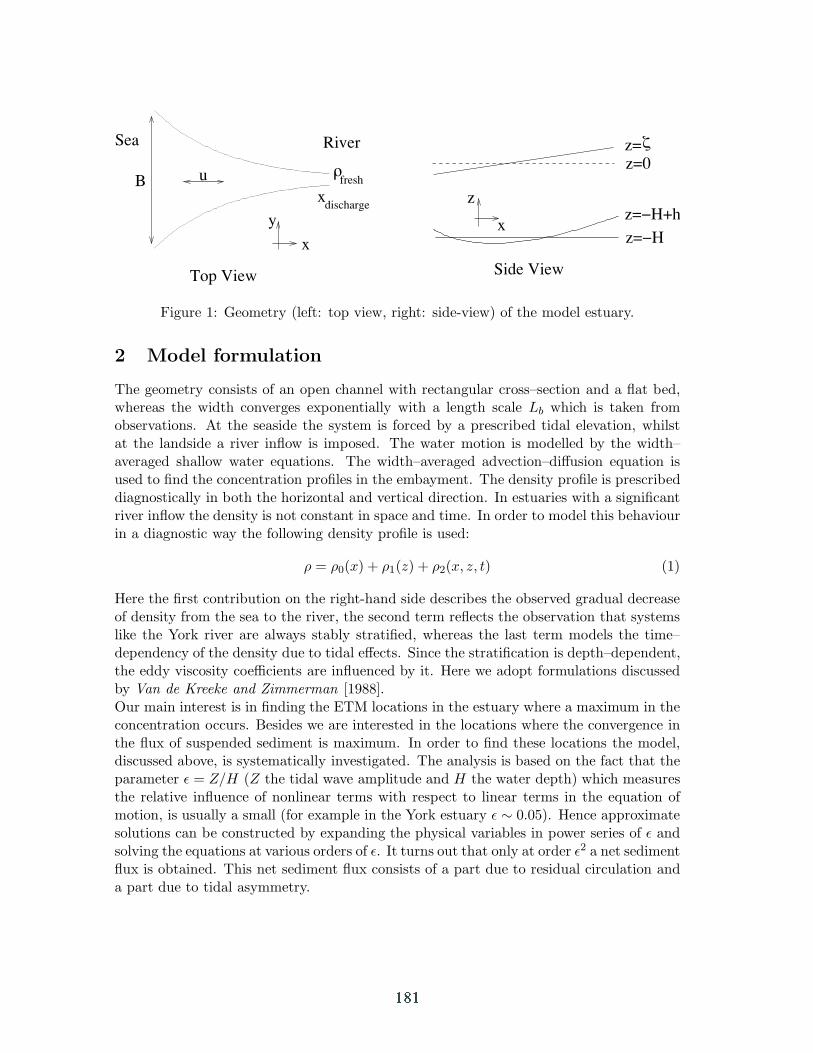
B

Sea River

x

y z=−H+h

Top View Side View

xdischarge

freshρ z=0

z=ζ

z

x

u

z=−H

Figure 1: Geometry (left: top view, right: side-view) of the model estuary.

2 Model formulation

The geometry consists of an open channel with rectangular cross–section and a flat bed,whereas the width converges exponentially with a length scale Lb which is taken fromobservations. At the seaside the system is forced by a prescribed tidal elevation, whilstat the landside a river inflow is imposed. The water motion is modelled by the width–averaged shallow water equations. The width–averaged advection–diffusion equation isused to find the concentration profiles in the embayment. The density profile is prescribeddiagnostically in both the horizontal and vertical direction. In estuaries with a significantriver inflow the density is not constant in space and time. In order to model this behaviourin a diagnostic way the following density profile is used:

ρ = ρ0(x) + ρ1(z) + ρ2(x, z, t) (1)

Here the first contribution on the right-hand side describes the observed gradual decreaseof density from the sea to the river, the second term reflects the observation that systemslike the York river are always stably stratified, whereas the last term models the time–dependency of the density due to tidal effects. Since the stratification is depth–dependent,the eddy viscosity coefficients are influenced by it. Here we adopt formulations discussedby Van de Kreeke and Zimmerman [1988].Our main interest is in finding the ETM locations in the estuary where a maximum in theconcentration occurs. Besides we are interested in the locations where the convergence inthe flux of suspended sediment is maximum. In order to find these locations the model,discussed above, is systematically investigated. The analysis is based on the fact that theparameter ε = Z/H (Z the tidal wave amplitude and H the water depth) which measuresthe relative influence of nonlinear terms with respect to linear terms in the equation ofmotion, is usually a small (for example in the York estuary ε ∼ 0.05). Hence approximatesolutions can be constructed by expanding the physical variables in power series of ε andsolving the equations at various orders of ε. It turns out that only at order ε2 a net sedimentflux is obtained. This net sediment flux consists of a part due to residual circulation anda part due to tidal asymmetry.

(a) (b)

(c) (d)

Figure 2: Time mean concentration for (a) and (c) a depth– and time–independent densityfield and (b) and (d) a depth– and time–dependent density field. Here the depth is scaledwith H = 10 m and the length with convergence length L = 70 km. In figures (a) and(b) no river outflow is present, whereas in (c) and (d) a river outflow of 0.54B0 m2 isprescribed with B0 the width at the entrance of the embayment. In figures (a) and (b)the arrows indicate the direction of the net sediment fluxes. These sediment fluxes areomitted in figures (c) and (d) since no convergence–divergence patterns can be discerned(large outward sediment flux due to river outflow).

3 Results and Discussion

In figure 2 the time averaged concentration fields are plotted for two different diagnosticallyprescribed density fields. In figures 2(a)–2(b) no river outflow is prescribed, whereas infigures 2(c)–2(d) a river outflow is present. It turns out that to get an estuarine turbitymaximum, it is essential for the density profile to have an inflection point, i.e. the along–estuary derivative of the density profile should have a maximum. This situation is shownin figure 2(a) where a density profile without any depth dependency and an inflectionpoint around L = 60 km is prescribed. Here the mechanism is due to an along–channel

baroclinic pressure gradient which sets up a density–driven circulation. If a depth– andtime dependency is added to the diagnostically prescribed density profile (so both ρ1 andρ2 are unequal to zero in (1)), it is possible to find situations in which more than one ETMis observed. Hence another mechanism resulting in particle trapping is the occurrence oftidal velocity asymmetry and its interaction with the time–varying concentration field.Usually a strong ETM is found around L = 60 km and a weaker one near the entrance ofthe estuary.

From these and other numerical experiments it can be concluded that during generallystratified conditions, one near–bed ETM is found. If the density stratification is assumedto be time–dependent as well (influence of tide), situations occur where two distinct ETMsoccur. Hence due to the phase lag between stratification and velocity another mechanismresulting in net convergence of suspended sediment is at work. The physical interpretationof this mechanism is presently under investigation. This seems to be consistent with fieldmeasurements where during more mixed conditions two instead of one ETMs are observed.However, the positions of the ETMs found in the model do not correspond very well withthe observations. Therefore, the dependence of the stratification on time and place willbe studied in more detail.

Furthermore, the strength of the ETMs is usually under–estimated. Therefore, analong–channel variable erosion will be studied in the near future as well.

References

Burchard, H., and H. Baumert, The formation of estuarine turbidity maxima due todensity effects in the salt wedge. a hydrodynamic process study, J. Phys. Oceanogr., 28 ,309–321, 1998.

Hansen, D., and M. Rattray, Gravitational circulation in straits and estuaries, J. MarineRes., 23 , 104–122, 1965.

Jay, D., and J. Musiak, Particle trapping in estuarine tidal flows, J. Geophys. Res., 99 ,445–461, 1994.

Lin, J., and A. Kuo, Downstream turbidity maximum in the york river, virginia, in 15thBiennial International Conference of the Estuarine Research Federation, 1999.

Nichols, M., and G. Poor, Sediment transport in a coastal plain estuary, J. Waterw.Harbors Div., ASCE , 93 , 83–95, 1967.

Van de Kreeke, J., and J. Zimmerman, Gravitational circulation in well- and partiallymixed estuaries, in Physical processes in estuaries, edited by J. Dronkers, and W. vanLeussen, pp. 495–521, Springer–Verlag, N.Y., 1988.

��

�� ! " �� #��$� ��

� ��

�� ! �� "�� #�� $�� %&'''()� "� �� *�� ! �� ! � ��

� �� %&'''( �� '+, � �� $� +�-�� ) � �� .+ � -+, � �� $� &�' �� )� �� #� �� / �� 0�� 1�� 2�� 0�� *� � ��

� ��

�� "�� 3�� $0�45') � �� $0� 674)� �� $8�� &) �� -+ � �� 9�� 9�� "�� #��0� �� "�� $� �� %&'':() � �� 8�� . �� $�� %&''+()�

�� Æ��

� � � !" �� #$�� %��&%�� %��

0 6 12 18 24

740 730

720 710

700

690

680

670

660

650

640630

H am burg

R h inp la tte

P agensand

S tade

S chw arz tonnen-sand

Stör

Bruns-bütte l

Oste

C uxhaven

m Depth

N orth S ea

G reatB rita in G erm any

D en-m ark

N

Elbe

0 1 2 3 4 5 1 0 km

9° 10°10 ' 20' 30' 40' 50'30 ' 40' 50 '

9° 10°10' 20' 30' 40' 50'30' 40' 50 '

54°

54°

30 '

40 '

50 '

54°

54°

30'

40'

50'

8�� &; �� "��< �� 0��

��

��

�

��

�

��

�

��

��

��

��

8�� .; ��

� ��

9�� "�� "�� $�� %&''+()� �� .4+ � ��*�� - � �� : �� ! �� =�� #�� $�� %&'''()� �� 0�� 0�� $� ��

�� %&''+() �� +�- $�� )� +�+5 $�� ) � +�++7 �� $��)$�� %&'''()� >�� # � �� 1�� 4++ ��

� �� 6�5 � �� ?�� 0�� #�� 0�� $+�++7 �� ) � �� 8 � �� 0�� $+�+5 �� )< �� #�� @� �� 0�� 8 �� <

�� 0 �� $?) � 0��:'+ � �� $>) � 0�� 6+4 � �� $� �� %&'':()� �� 0 $") � �� 0 $8) � ��

� ��75

8085

9095

100

Simulation

[ % ]

DF DE UF UE

FVS

8�� -; �� 7 ��

8�� - �� 7 �� 8� �� 0�� $@) �� 0�� $8)�

05

1015

Simulation

[ sq

km ]

DF DE UF UE

FVS

−2

01

23

4

Simulation

[ km

]

DF DE UF UE

FVS

8�� 7; "�� 4+ , � �� 7 �� $��) � �� < �� $��)�

>�� 0�� 4+ , �� $8�� 7� �� )� @�� ? $+�: � .�5 0��) �� >

$-�4 � &4 0��)� /� �� $&�- � &4 �� +�: � &+�5 0��)� 9��0�� 8 $�� .�- �� )� "�� @ $+�64 � +�' � �� 8)�9�� $8�� 7� �� )�� < �� 8 � �� "� "�� >�� @ �� +�4 0� � �� +�44 0�� 8 �� .�4 �-�' 0� �� < �� &�.: � &�4 0� ��A�� -�: 0� � �� +�44 0�� B�� &�7 0�� 8�� @ �� .�. � .�4 0� �� &�4 0� �� ?"�� 0�� 0�� 0�� 0�� C� �� #�� C��

��

D�� E�� 3� �� 2� D�� 2�#?� 8�� #�� #�� "�� #�� !�"�� #$� -.-#--.� &'':�

D�� E�� D� >�� !�� "�� %�� &�� '��"�� !�� F�� -4#7+� ��@�� G�� &''+�

�� F�� !� =�� /� !H�� !� ��H�� 2� DH�� #�� %��

&�� '��"�� !�� F�� &:4#&6&� �� @�� G�� &''+�

��0�� B� �� >�� !�� "��;>�� =�� ! �� E� 3�� ()#� 9&&� .:�+7-#.:�+46� &'''�

F�� D� � D�� =�� 9�� "��; �� *�� +(� 7�74-I7:-� &'''�

188

Bottom fine sediment boundary layer and transportprocesses within the turbidity maximum of the ChangjiangEstuary, ChinaZHONG SHI

(Department of Harbour and Coastal Engineering, School of Naval Architecture and OceanEngineering, Shanghai Jiao Tong University, 1954 Hua Shan Road, Shanghai 200030,People’s Republic of China, [email protected])

1. Introduction

A turbidity maximum zone has been found in many turbid estuarine environments (e.g., the GirondeEstuary, France, Glangeaud [1938]; the Chesapeake Bay, USA, Schubel [1968]; the Weser Estuary,Germany, Wellershaus [1981], Grabemann et al. [1995]; the upper Saint Lawrence Estuary, Canada,Lang et al. [1989]; the Tamar estuary, UK, Uncles and Stephens [1993]; the Hawkesburry Riverestuary, Australia, Hughes et al. [1998]; the Seine Estuary, France, Brenon and Le Hir [1999]).Several mechanisms govern the fine suspended sediment transport in the turbidity maximum: 1)flocculation, 2) estuarine circulation, 3) tidal pumping, 4) flood/ebb tidal asymmetry, 5) wind, and 6)turbulence suppressions of fine suspended sediment/salinity stratifications.

The Changjiang (Yangtze) is the fourth largest river in terms of both water and sediment discharge inthe world. The Changjiang Estuary is a mesotidal estuary with mean tidal range of 2.8 m. More than90% consists of fine sediments (<32 mµ ) in the Changjiang Estuary. It provides a good example of awell developed turbidity maximum (Li and Zhang [1998]; Shi [2002]). A number of questions need tobe addressed regarding the generation and maintaining of the turbidity maximum in the ChangjiangEstuary.

Aims of this paper are 1) to examine the spring/neap tidal, intratidal (flood/ebb), and burst-typestructures of bottom fine sediment bounary layer; 2) to correlate those structures (average andinstataneous) to dynamic processes such as tides, waves, and fine sediment density currents; and 3) toelucidate the dominant physical processes generating and maintaining the turbidity maximum at themouth of the Changjiang Estuary, China.

Figure 1: The Changjiang Estuary and monitoring station 9410.

189

2. Field Observations and MethodsMeasurements (acoustic profiling) were also made at station 9410 (122o27'30"E, 310o5'36"N, Figure1) during spring tide (0600 hr 07 October 1994_0700 hr 08 October 1994), moderate tide (1100 hr 13October 1994_1500 hr 14 October 1994) and neap tide (1400 hr 15 October 1994_1700 hr 16 October1994). Vertical profiles of fine suspension concentration were measured by an acoustic suspendedsediment monitor (Shi et al. [1999]). Tidal current speed and direction were measured hourly at 0.1 D,0.2 D, 0.4 D, 0.6 D, 0.8 D and 1.0 D (D: water depth above the bottom) using an electromagneticcurrent meter. Time series data of current velocity, salinity and suspended sediment concentrationwere measured at spring and neap tides in the Changjiang Estuary.

3. Results and DiscussionA turbidity maximum was consistently observed at the mouth of the Changjiang Estuary during springtide (Figure 2). Those data were analyzed for (1) spring/neap tidal, (2) intratidal (flood/ebb), and (3)burst-type dynamic nature of fine suspended sediment transport processes within the turbiditymaximum there.

Figure 2: Acoustic images of burst-averaged concentration over a 12-min period for each hour during spring tide(0600 hr 07 October 1994_0500 hr 08 October 1994). Bottom bar: burst-averaged concentration.

Calibrated acoustic images (Figure 2) revealed that: (1) bottom fine sediment boundary layer; (2) theevolution of the fine suspension concentration profiles to tide-, wave- and fine sediment density-induced forcing; (3) turbulence suppression by salinity/concentration stratification is one of theimportant mechanisms for the formation of turbidity maximum; (4) impulsive fine sedimentresuspension by bottom fine sediment boundary-induced currents; and (5) Kelvin-Helmholtzinstability is one of the dominant processes responsible for the re-entrainment of the near-bed highconcentration suspension. Furthermore, coherent structures were present in the fine sediment boundarylayer (2400 hr, 08 October 1994). The structure of a bottom sediment boundary layer was studied incentral Long Island Sound by Bedford et al. (1988). Fine sediment-induced density currents areresponsible for fine suspended sediment transport processes (Figure 2). The coupling between finesediment bed and fine suspension in the bottom boundary layer is important, as discussed by Boudreau[1997].

190

4. ConclusionField observations have been made to examine the spring/neap tidal, intratidal (flood/ebb), and burst-type dynamic natures of bottom fine boundary layer and suspended sediment transport processes at themouth of the Changjiang Estuary. Fine sediment-induced density currents and others are responsiblefor fine suspended sediment transport processes in the turbidity maximum at the mouth of theChangjiang Estuary.

Acknowledgments: This research was funded by the National Natural Science Foundation of China (Estuarineand Coastal Program, No. 49806005).

References:

Bedford, K.W., Libicki, C., Wai, O., Abdelrhman, M. and Van Evra, R., The structure of a bottomsediment boundary layer in central Long Island Sound. In: J. Dronkers and W. van Leussen (Eds.),Physical Processes in Estuaries. Springer-Verlag Berlin Heidelberg, Germany, 1988, 446-462.

Boudreau, B.P., A one-dimensional model for bed-boundary layer particle exchange. Journal ofMarine Systems, 11, 279-303, 1997.

Brenon, I. and Le Hir, P., Modelling the turbidity maximum in the Seine Estuary (France):identification of formation processes. Estuarine, Coastal and Shelf Science, 49, 525-544, 1999.

Glangeaud, L., Transport et sedimentation clans l’estuairc et a l’embouchure de La Gironde. Bulletinof Geological Society of France, 8, 599-630, 1938.

Grabemann, I., Kappenberg, J. and Krause, G., Aperiodic variations of the turbidity maximum of twoGerman coastal plain estuaries. Netherlands Journal of Aquatic Ecology, 29 (3-4), 217-227, 1995.

Hamblin, P.F., Observations and model of sediment transport near the turbidity maximum of the upperSaint Lawrence estuary. Journal of Geophysical Research, 94 (C10), 14,419-14,428, 1989.

Hughes, M.G., Harris, D.T. and Hubble, T.C.T., Dynamics of the turbidity maximum zone in a micro-tidal estuary: Hawkesburry River, Australia. Sedimentology, 45, 397-410, 1998.

Li, J.F. and Zhang, C., Sediment resuspension and implications for turbidity maximum in theChangjiang Estuary. Marine Geology, 148: 117-124, 1998.

Schubel, J.R., Turbidity maximum of the Northern Chesapeake Bay. Science, 161, 1013- 1015, 1968.

Shi, Z., Dynamics of the turbidity maximum in the Changjiang Estuary, China, in J.C. Winterwerp andC. Kranenburg (Eds.), Proceedings of the 6th International Conference on Nearshore and EstuarineCohesive Sediment Transport Processes, September 4-8, 2000, WL/Delft Hydraulics, Elsevier MarineSciences, The Netherlands, 2002: in press.

Uncles, R.J. and Stephens, J.A., Nature of the turbidity maximum in the Tamar estuary, U.K.Estuarine, Coastal and Shelf Science, 36, 413-431, 1993.

Wellershaus, S., Turbidity maximum and mud shoaling in the Weser estuary. Archiva Hydrobiologica,92, 161-198, 1981.

��

�� ! " � �� #��

�� $ �� %� &�� ' ��(��)�� %�� *!� ��

*+**" &��,� #��

� ��

�� !�� !�� !�� "� �� " �� !�� "� �� #��

�� !�� $ �� !�� %��" �� ""�� !�� &'' $� �� Æ� � �� "�� $�� "�� (� �� )�� "�� )�� #�� !�� *� �� ( )�� +��,�� (�� !�� -' $� �� "� �� )��

�� !�� "�� #�� " � � !�� +�� "� �� "� � � ��

� � � ��

�� .!�� .�� !��

�� /-''-0� � � 12 �� *�� " �� "�� " #�� " ��"�� 3�� !�� 1� �� /&4540 � ��6�� /&4440 � �� 6�� . ��

�� /&4440 � �� (��"� �� !�� ""�� /&4450�7�� "�� "�� 8 � � �� " �� " �� 9�� 1� �� "�� *� �� #�� $�

� � Æ�� -�� /&4450 �� " � � !�� ""�� $�� /&44:0�� 9�� "�� 9�� !�� !�� ;�� "�� *�� .<�� .�� <�� 7==��"�� .!�� (�� "�*�� *�� " ��

� �� "�� #�� #� �� 7

�� >�� ? �� &�

� �� ; �� $ �" �� !�� *�� #�� " �� /&4@-0 �� 9 �� ( �� + � �� $� �� #� � ��

� ��

6� �� "�� "�� "�� *� �� " � � !�� !�� *� � �� /&4450 �� -� �� *�� !�� *� �� ( -2 �� "�� A?&'' $� �� &B � � �� !�� " �� - � �� &�1 � �� *�� C'' �� 9�� !�� 1' �� )�� ?��?-'' � �� 1' �9 � �� )?'�B �� " � � �� !�� "�� 6� �� "��&�� 6� � ��

�� *� � �� 1� �� &'' $� ��" ��

3 "�� &7 �� - �� 1'� �� B' $� � �� -� �� ( $*� ��

�� "�� & $� �� 5 $� �� &B � �� (��" �� )�� "�� !�� *� � �� -��*�� )�� #�� (�� !�� "� �� -� �� <�� " �� " � �� *�� *�� " #�� #�� !��

3 �� !�� (� �� " �� !��

��

�� !""""#"$%� &��'

��

�� (�� )��

��

+�� A�% � �� " �� 3��7�� ! B-B*B:: &444�

+�� %� �� %� +�� 3�� !�� 2�� !�� 6��"�� ( %�� "�� #�� $% 1'4*1-& &445�

+�� %� �� D� +�� " .!�� "�� E�� !FE -'-B1 !G !�� ;�� &BC �� -''-�

;�� A� �� E� G�� %�� " � ��*�� 7 (�� 6�� . ��

�� $$ &&C*&1& &444�

H�� 2� �� H� 2� �� $ �� " � �� #�� &�'�� (�� !! ::B*:@& &44:�

D�� E� +� 3�� " ��3 �� E�� %�� !�"� A�� F� (�� ;�� !�"� &&' �� &4@-

A��" .� E� �� $��$� %*F� 3��"�� .�� %�A�D�� A�H�E�G�� E� E ��,�� 2�� " � �� &45B �� &�'�� (�� ! &:15&*&:141 &454

195

Sediment flux and budget on tidal to decadal time scales ina sandy, macrotidal estuaryCOLIN JAGO, SARAH JONES, GARRY REID, KADIR ISHAK

(School of Ocean Sciences, University of Wales Bangor, Marine Science Laboratories, MenaiBridge, Gwynedd, LL59 5EY, UK, [email protected])

1. IntroductionEstuaries on macrotidal coastlines are characterised by large sediment fluxes due to tidal currents andby net sedimentation resulting from differences in flood and ebb transports. Quantification of sedimentbudgets on time scales of years to decades is important for effective management with respect to, forexample, ecosystem sustainability, water quality, and navigation. Appropriate datasets on such timescales are rare. However, the advent of technologies for high frequency measurement of currents andsuspended sediment concentrations provides the potential for high resolution estimation of netsediment flux on short time scales and, hence, for extrapolation of sediment budgets on longer timescales. But, as emphasised by McCave [1979], the validity of net sediment fluxes determined frommeasurements is questionable since flood and ebb fluxes are very large numbers with largemeasurement error bars and the net flux is a relatively small number. Attempts to measure netsediment fluxes have been constrained by such uncertainties: see Terwindt [1967](Rhine), Fleming[1970] (Clyde), Allen and Castaing [1973] (Gironde), Harris and Collins [1988] (Bristol Channel),Hardisty and Rouse [1996] (Humber). Uncertainties become limiting where the net flux is a very smallproportion of the gross flux � for example, 1% in the Humber estuary. Here we describe an attempt toquantify annual sediment budgets, independently measured on a decadal time scale, by short termmeasurement of sediment fluxes in an estuary where the net flux is about 10% of the gross flux.

2. Field siteThe macrotidal Taf estuary in SW Wales, UK is 1.5 km wide at its mouth narrowing down to lessthan 10 m at the farthest intrusion of salt water, 15 km from the mouth. The estuary is dominated bytidal forcing (see Jago [1980]). The tidal range is large, reaching 10 m on a big spring tide. Tides showtime-velocity asymmetry particularly on springs when the flood is < 3 hours and fast currents pulsingto 2.5 m s-1 are generated. On springs the ebb is about 4.5 hours long, after which the estuary iseffectively void of salt water. The river Taf is small with a daily average discharge of 7 m3 s-1. Theestuary is protected from swell waves due to a sand spit across its mouth.

The extended period (4.5 hours) when salt water is excluded from the estuary is characterised by ameandering channel (usually < 1 m deep) which cuts through extensive areas of intertidal sand flatsbordered in places by narrow mud flats and saltmarsh. The sand flats are the most extensivephysiographic unit and are characterised by well sorted, fine sand (mean grain size 130 µm) whichshows little spatial variation. Mineralogical analysis proves that the estuarine sands are derived fromoffshore and not from the River Taf (see Jago [1980]). These sands are readily entrained by the tidalcurrents which generate shear velocities exceeding 0.15 m s-1 on big spring tides. The fine sands areentrained directly into suspension with little bed load transport.

3. Methods

Sediment budget

Ten transects were set up across the estuary in 1968 between temporary bench marks fixed in the

196

saltmarsh at both ends of each transect. Transects were spaced between the estuary mouth and thelandward limit of the intertidal sand flats. Profiles along transects were determined by conventionallevelling, at low tide when the estuary is traversable on foot, intermittently between 1968 and 1980,annually between 1981 and the present (35 surveys of each transect in total). Profile changes werespatially integrated to quantify gross changes between surveys and hence to determine thesedimentation rate on the sand flats (sand volume change/sand flat area).

Sediment flux

Short term flux measurements were made along two of the levelling transects across the estuary.Simultaneous measurements of velocity and suspended sediment concentration (SSC) were made atfixed stations, about 150 m apart, on the transects over several (up to 6) tidal cycles. Currentvelocities were measured using velocity gradient units (each with 10 impellors) at 2 sites on eachtransect; data were logged as 1 minute averages every 10 minutes. Velocities at other stations weremeasured with EM and impeller current meters deployed every 15 minutes in profiling mode fromanchored boats.

SSC was measured using a 0.1 m path length SeaTech transmissometer linked to an AppliedMicrosystems STD-12, and was deployed in profiling mode from a fast inflatable boat whichtraversed a transect and visited each site every 10 minutes. Data were logged at 0.1 m depthincrements. The transmissometer was calibrated in situ by comparison with 500 ml water samplesfiltered through washed, preweighed Whatman GF/C glass microfibre filters. Blank filters wereused to determine the accuracy of the gravimetric procedures: the error was less than 0.3%.

4. Results

Sediment budget

While individual transects experienced variable sedimentation and erosion, integration of changes onall transects showed a progressive increase of sand in the estuary. During the period 1968-97, therewas a gain of 2.94x106 m 3 of sand due to an annual influx of c. 0.10x106 m 3. This gain gave rise to anannual mean sedimentation rate of 0.02 m. Given the mineralogical evidence, this represents a netinput of marine sand from offshore and is the budget that has to be matched by the budget estimatedfrom the flux measurements.

Sediment flux

There was a large variation in SSC at the sampling stations. High values, up to 1000 mg l -1, occurredduring peak flows but reduced to 10 mg l -1around slack high water. Two orders of magnitudevariation in SSC posed some problems with transmissometer calibration as there was a variation inparticle size over a tidal cycle. Deployment of a LISST 100 laser sizer showed that suspendedsediment was more than 80% fine sand during most of the flood and ebb, but at high water the sandfraction dropped out of suspension leaving finer particles (mode < 20 µm). Although the values ofSSC around slack high water, after sand had been deposited, did not significantly impact on sedimentflux estimates, separate calibration curves for sand and fine fractions were generated. Calibrationcoefficients (R2) ranged 0.58-0.89 with lower R2 values for sand because of the difficulties ofobtaining simultaneous transmissometer readings and water samples in the rapidly changingconditions of the early flood and late ebb tides.

Much of the sediment flux during a tidal cycle occurred at the start of the flood tide (as the rapidlyrising tide poured into the estuary) and towards the end of the ebb (as flow became confined to themain channel). Typical values of gross sediment flux per tide were 0.79x105 kg and 22.40x105 kg for

197

neaps and springs, respectively. While at some stations along transects, ebb sediment flux exceededflood sediment flux (because flood and ebb channels did not coincide), overall flood sediment fluxexceeded ebb sediment flux on all tides. Typical values of net sediment flux per tide were 0.19x105 kgand 1.88x105 kg for neaps and springs, respectively. Hence net flux, always landward, was an order ofmagnitude greater on springs than on neaps.

There were exponential relationships between sediment flux per unit width of transect and tidal rangewith R2 values of 0.88 and 0.90 (95% confidence) for flood and ebb tides, respectively (Figure 1).These gave the following when data from both transects were combined:

Fflood = 19.20 x 2.17t

Febb = 9.67 x 2.17t

where F = sediment flux (kg m-1) and t = tidal height above O.D. (m)

Figure 1: Relationships between sediment flux per metre width and tidal height

Errors were in part due to measurement errors: e.g. transmissometer calibration; water fluxmeasurement (typically 0-5%). There was inherent variability during early flood and late ebb tideswhen measurement was most difficult due to problems of small boat handling in shallow, turbulentwaters. Nevertheless, these errors were small. Further contributions to errors are the absence of anyother processes (especially river discharge) in the algorithms. River discharge contributes to sedimenttransport during the period of sand flat exposure when river flow generates a seaward sediment flux.

The algorithms were used to compute total sediment fluxes over a year. And these fluxes were used tocompute net sedimentation rate over the sand flats landward of each transect. With 40% porosity forthe deposited sand, this gave sedimentation rates of 0.016 ± 0.046 m yr-1 and 0.012 ± 0.026 m yr-1 ineach case. The error bars are 95% confidence limits around the defining algorithms. These estimatescompare very favourably with the `true´ value (0.020 m yr-1) given by the long-term levelling surveys.

5. Conclusions

The long-term levelling dataset provided an unusual opportunity for testing the validity of netsediment flux estimated from in situ measurements over short periods. While the experiment started

Ebb tides

0

200

400

600

800

1000

1200

1400

2.5 3.5 4.5 5.5

Tidal height above OD m

Sed

imen

t fl

ux

kg/m

wid

th

Flood tides

0

200

400

600

800

1000

1200

1400

2.5 3.5 4.5 5.5

Tidal height above OD m

Se

dim

en

t fl

ux

kg

/m w

idth

198

with the premise that short term measurements cannot be used to determine sediment budgets, for thereasons given by McCave [1979], in fact the annual sediment budget extrapolated from the fluxmeasurements was remarkably close to the budget determined from the 30 yr levelling dataset. Theconclusion must be that, for this estuary, the mean annual sedimentation rate can be realisticallydetermined from flux measurements over a few tidal cycles. However, there are specific reasons whyMcCave�s strictures have proved to be unfounded in this particular case. Bedload transport isnegligible in the Taf estuary so that SSC is a valid parameterisation of sediment transport ; sosediment flux can be measured relatively easily. Furthermore, the uniformity of sand texture meansthat transmissometer calibrations are spatially and temporally robust. Finally, the time-velocityasymmetry of the tide gives rise to a large net sediment flux which is c.10% of the gross sedimentflux. The net flux therefore lies outside the error bars of in situ measurement.

References

Allen, G.P., Castaing, P., 1973. Suspended sediment transport from the Gironde estuary (France) ontothe adjacent continental shelf. Mar.Geol., 14, M47-M53.

Flemming, G.,1970. Sediment balance of the Clyde estuary.J.Hydraul.Div.Proc.Amer.Soc.civil Eng.,96, 2219-2230.

Hardisty, J.G., Rouse, H.L., 1996. The Humber Observatory: Monitoring, modelling and managementfor the coastal environment. J.Coastal Res.,12, 683-690.

Harris, P.T., Collins, M., 1988. Estimation of annual bed load flux in a macrotidal estuary: BristolChannel, U.K. Mar.Geol., 83, 237-252.

Jago, C.F., 1980. Contemporary accumulation of marine sand in a macrotidal estuary, SouthwestWales. Sediment.Geol., 26, 21-49.

McCave, I.N., 1979. Suspended sediment. In: Dyer, K.R. (Ed.), Estuarine Hydrography andSedimentation. Cambridge Univ. Press, pp. 131-185.

Terwindt , J.H.J., 1967. Mud transport in the Dutch Delta area and long the adjacent coastline.Neth.J.Sea Res., 3, 505-531.

199

Sediment Flux at the Mouth of the Humber EstuaryJACK HARDISTY

(Department of Geography, The University of Hull, HU6 7RX UK and NorthSea SoftwareSystems Ltd. Barkers Mill, Beverley, HU17 0UJ, UK [email protected])

1. IntroductionThe Humber Estuary on the east coast of northern England drains some 24,000 km2 and has a tidalprism in excess of 1.5km3. Although recent work shows that the estuary has been accreting at a rate ofabout 1 MT a-1 throughout the last 5,000 years since sea level attained its current elevations, sedimenttransport processes at the estuary mouth are essentially symmetrical with some 100 kT of suspendedsolids carried inwards and outwards on each flood-ebb cycle (Hardisty, et al., 1998, Dyer, et al.,2000). Results from the Humber Flux Curtain experiment are reported which describe the seasonal,inter- and intra-tidal variations in sediment flux and also quantify the effects of changing riverdischarge and demonstrate that net fluxes due to these processes are negligible.

-2.00

-1.00

0.00

1.00

2.00

3.00

4.00

5.00

6.00

7.00

8.00

0 1 0 2 0 3 0 4 0 5 0 6 0 7 0 8 0 9 0 100 110

0

200

400

600

800

1000

1200

1400

1600

1800

2000

0 1 0 2 0 3 0 4 0 5 0 6 0 7 0 8 0 9 0 100 110

Figure 1: Water depth (upper diagram) and suspended particulate matter (lower diagram) at the mouth of theHumber Eastuary for the first five days of 1996.

2. Flux Curtain ExperimentData were collected throughout 1995-1997 from radio linked instrument systems moored across themouth of the Humber Estuary measuring water temperature, salinity, depth, suspended particulatematter (SPM) and flow velocities. The relationship between the SPM and tidal range and freshwaterforcing is examined as shown in Figure 1.

3

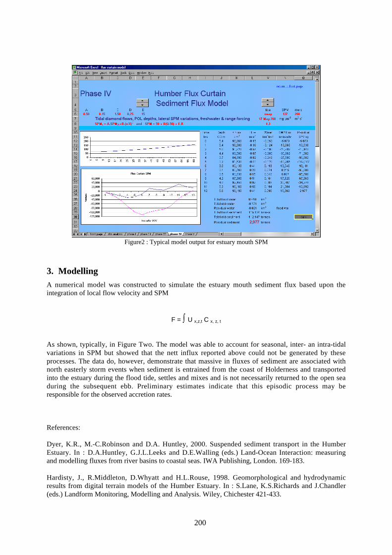
200

Figure2 : Typical model output for estuary mouth SPM

3. ModellingA numerical model was constructed to simulate the estuary mouth sediment flux based upon theintegration of local flow velocity and SPM

F = ∫ U x,z,t C x, z, t

As shown, typically, in Figure Two. The model was able to account for seasonal, inter- an intra-tidalvariations in SPM but showed that the nett influx reported above could not be generated by theseprocesses. The data do, however, demonstrate that massive in fluxes of sediment are associated withnorth easterly storm events when sediment is entrained from the coast of Holderness and transportedinto the estuary during the flood tide, settles and mixes and is not necessarily returned to the open seaduring the subsequent ebb. Preliminary estimates indicate that this episodic process may beresponsible for the observed accretion rates.

References:

Dyer, K.R., M.-C.Robinson and D.A. Huntley, 2000. Suspended sediment transport in the HumberEstuary. In : D.A.Huntley, G.J.L.Leeks and D.E.Walling (eds.) Land-Ocean Interaction: measuringand modelling fluxes from river basins to coastal seas. IWA Publishing, London. 169-183.

Hardisty, J., R.Middleton, D.Whyatt and H.L.Rouse, 1998. Geomorphological and hydrodynamicresults from digital terrain models of the Humber Estuary. In : S.Lane, K.S.Richards and J.Chandler(eds.) Landform Monitoring, Modelling and Analysis. Wiley, Chichester 421-433.

201

Factors affecting longitudinal dispersion in estuaries ofdifferent scaleROY LEWIS

(Brixham Environmental Laboratory, AstraZeneca UK Limited, Freshwater Quarry, Brixham,Devon, TQ5 8BA, U.K., [email protected])

REG UNCLES

(Plymouth Marine Laboratory, Prospect Place, West Hoe, Plymouth, Devon, PL1 3DH, U.K.,[email protected])

1. IntroductionTo assess the biological health of a given estuary, it is usual to compare the biological conditions withthose in similar systems. This leads to the problem of deciding what aspects of the physical, chemicaland biological characteristics make any two systems ‘similar’. A key factor that indicates whether twoestuaries are physically similar is the degree of dilution obtained by dissolved substances; this is notsimply a measure of the overall capacity of the estuary but rather its ability to dilute and flush to seaany soluble substances entering the system.

The distribution of salinity of estuarine waters has long been used as an indicator of the dilutingcapability of the system. It is generally relatively easy to obtain salinity data for an estuary, especiallyif the salinity distribution can be measured without the need for anchored stations. Furthermore, thesalinity distribution in an estuary is a useful overall indicator of the physical condition of the systembecause it represents the resultant effect of numerous complex processes - freshwater inflow, tidalrange, velocity variations (spatial and temporal) and the degree of turbulence.

The approach adopted in this study is to develop a solution for the mass balance equation for saltunder the assumption that estuaries tend to an equilibrium situation in which the loss of salt from thesystem by freshwater transport is matched by an upstream ‘diffusive’ flux due to non-advectiveprocesses. The model assumes that each estuary cross-section expands exponentially towards the seaand that, averaged over an appropriate period of time, the longitudinal dispersion coefficient isessentially constant in each system. In most instances, it is further assumed that this coefficientremains constant along the estuary length.

2. Data SetsThe data used in the analysis came from observations in five UK estuaries. These estuaries range insize and in cross-sectional form; for example, the reclamation and canalisation of the Tees estuary hasgreatly reduced the area of the intertidal mudflats, while the Tamar estuary retains extensivemudbanks at low water. Although the five estuaries were principally selected because of the quality ofthe data, it was seen as desirable that the systems should span a range of scales, so that any effects ofscale differences could be noted.

The approach adopted for the analysis is really for well mixed systems in which the depth meansalinity deviates little from the surface and bed distributions. However, some of the data sets forpartially- mixed estuaries, such as the Tees or the Tamar, were sufficiently sound and comprehensiveas to merit their inclusion.

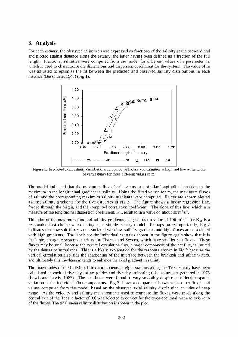
202

3. AnalysisFor each estuary, the observed salinities were expressed as fractions of the salinity at the seaward endand plotted against distance along the estuary, the latter having been defined as a fraction of the fulllength. Fractional salinities were computed from the model for different values of a parameter m,which is used to characterise the dimensions and dispersion coefficient for the system. The value of mwas adjusted to optimise the fit between the predicted and observed salinity distributions in eachinstance (Bassindale, 1943) (Fig 1).

Figure 1: Predicted axial salinity distributions compared with observed salinities at high and low water in theSevern estuary for three different values of m.

The model indicated that the maximum flux of salt occurs at a similar longitudinal position to themaximum in the longitudinal gradient in salinity. Using the fitted values for m, the maximum fluxesof salt and the corresponding maximum salinity gradients were computed. Fluxes are shown plottedagainst salinity gradients for the five estuaries in Fig 2. The figure shows a linear regression line,forced through the origin, and the computed correlation coefficient. The slope of this line, which is ameasure of the longitudinal dispersion coefficient, Kxe, resulted in a value of about 90 m2 s-1.

This plot of the maximum flux and salinity gradients suggests that a value of 100 m2 s-1 for Kxe is areasonable first choice when setting up a simple estuary model. Perhaps more importantly, Fig 2indicates that low salt fluxes are associated with low salinity gradients and high fluxes are associatedwith high gradients. The labels for the individual estuaries shown in the figure again show that it isthe large, energetic systems, such as the Thames and Severn, which have smaller salt fluxes. Thesefluxes may be small because the vertical circulation flux, a major component of the net flux, is limitedby the degree of turbulence. This is a likely explanation for the response shown in Fig 2 because thevertical circulation also aids the sharpening of the interface between the brackish and saline waters,and ultimately this mechanism tends to enhance the axial gradient in salinity.

The magnitudes of the individual flux components at eight stations along the Tees estuary have beencalculated on each of five days of neap tides and five days of spring tides using data gathered in 1975(Lewis and Lewis, 1983). The net fluxes were found to vary smoothly despite considerable spatialvariation in the individual flux components. Fig 3 shows a comparison between these net fluxes andvalues computed from the model, based on the observed axial salinity distribution on tides of neaprange. As the velocity and salinity measurements used to compute the fluxes were made along thecentral axis of the Tees, a factor of 0.6 was selected to correct for the cross-sectional mean to axis ratioof the fluxes. The tidal mean salinity distribution is shown in the plot.

203

Figure 2: Plot of maximum net flux of salt against maximum salinity gradient.

In Fig 3 it can be seen that the predicted net flux from the model is of similar magnitude to theobserved flux at the six most seaward stations in the diverging estuary; these span a distance of about11 km. Only at the two landward stations does the difference between the observed and predictedfluxes become significant. This deviation is at least partially due to errors in the fluxes computed fromthe measurements because, at that part of the estuary, they represent relatively small differencesbetween large terms.

The model was used to demonstrate that, allowing for a small increase in the freshwater flow, therewas still a seaward shift in the depth mean salinity distributions between periods of neap and springtides. This neap to spring change is associated with a reduction in the maximum landward flux of salt.As the model assumes an equilibrium between non-advective flux and freshwater advection, anyreduction in the landward salt flux is balanced by a seaward shift in the overall salinity distribution.The displacement in the salinity distribution means that, for a given salinity, the cross-sectional areaincreases so that the seaward advective transport of salt per unit area decreases. The new location ofthe salinity distribution represents the location at which this transport again balances the non-advectivetransport of salt.

Figure 3: Comparison of the predicted net flux of salt with the observed fluxes along the Tees estuary. Thecorresponding observed tidal and depth mean salinities, expressed as fractions of the salinity at the estuary

mouth are also shown.

204

4. ConclusionsA steady state model, that assumes an exponential increase in estuary area with distance towards thesea and a constant value for the longitudinal dispersion coefficient, indicates that the maximumlandward flux of salt occurs in the vicinity of the maximum axial gradient in salinity.

Data sets selected for their quality were used to compute matching pairs of values for the maxima insalt fluxes and salinity gradients. A plot of these variables indicated that lower fluxes and salinitygradients were associated with the larger, more energetic, estuaries. A linear fit through the datasuggested that a value of 100 m2 s-1 for the longitudinal dispersion coefficient, Kxe, is reasonable firstestimate for estuary mixing problems.

Studies of the net fluxes associated with the salinity distributions for the Tees estuary indicated that, ifthe landward flux becomes too small to counter the seaward advection of salt by river flow, thesalinity distribution shifts to a region of greater cross-section, so that the upstream ‘diffusive’ flux ofsalt again balances the freshwater advection per unit area.

References:

Bassindale, R., A comparison of the varying salinity conditions of the Tees and Severn estuaries.Journal of Ecology, 12 (1), 1-10, 1943.

Lewis, R.E. and Lewis, J.O. The principal factors contributing to the flux of salt in a narrow, partiallystratified estuary. Estuarine, Coastal and Shelf Science, 16, 599-626, 1983.

205

Salt intrusions in Siberian River Estuaries -Observationsand model experiments in Ob and YeniseiINGO H. HARMS, UDO HÜBNER, JAN O. BACKHAUS

(Institute for Oceanography, University Hamburg, Troplowitzstrasse 7, 22529Hamburg,Germany, harms @ifm.uni-hamburg.de)

MIKHAIL KULAKOV, VLADIMIR STANOVOY

(Arctic and Antarctic Research Institute, Bering Strait 38, 199397 St. Petersburg, Russia,[email protected])

OLEG STEPANETS, LUDMILLA KODINA

(Vernadsky Institute of Geochemistry, Kosygin Strait 19, 117975 Moscow, Russia,[email protected])

REINER SCHLITZER

(Alfred-Wegener-Institute for Polar and Marine Research, Columbusstrasse, 27568Bremerhaven, Germany, [email protected])

1. ObservationsCompared to other Arctic Shelf Seas, the Kara Sea receives large amounts of freshwater through theSiberian rivers Ob and Yenisei. Both rivers drain a catchment area in Siberia and Russia of more than5 mill. km2. The total annual amount of freshwater input into the Kara Sea equals roughly 1200 km3/yof which 80% is discharged in spring (May - June) [Pavlov and Pfirman, 1995]. Peak discharge ratesof more than 100.000 m_/s lead to a pronounced vertical stratification which is additionally enhancedby atmospheric warming and ice melting.

Historical data showed a permanently existing pycnocline in the estuary of Ob and Yenisei but recentCTD-profiles revealed that vertical salinity and temperature gradients in the Yenisei Estuary may beextremely strong and reach values of up to 5-10 psu per 10 cm and 1.5 � 2.0 °C per 10 cm (Fig. 1).These extreme situations can be observed when due to strong wind induced off-shore surface flow,high saline bottom water penetrates into the estuary, leading to so called �salt intrusions�. The datashow that salt intrusions occur most probably during summer, in August or September, when north-easterly winds prevail and the difference between upstream surface salinity and downstream bottomwater salinity is most pronounced.

50 100 150 200 250 300

Distance, km

-30

-20

-10

0

Dep

th, m

78 80 82 8470

71

72

73

Fig. 1: Salinity section in the Yenisei estuary, summer 1995

206

2. Model applicationAt the Institute for Oceanography, University Hamburg, the shelf sea modelling group applies a highresolution baroclinic 3-d circulation and sea ice model to the Kara Sea. The horizontal grid resolutionis 9.4 km. The model is based on the coding of the Hamburg Shelf Ocean Model HAMSOM,introduced by Backhaus [1985], and previously applied to the Barents and Kara Sea by Harms [1997a,b]; Harms and Karcher [1999] and Harms et al. [2000]. The circulation model is coupled to athermodynamic and dynamic sea ice model, which calculates space and time dependent variations ofice thickness and ice concentration [Hibler, 1979].

Our present studies are forced with with realistic atmospheric winds, heat fluxes, river runoff andtides. In order to handle complex bathymetries and to reproduce more realistically topographic effectson circulation and hydrography, the coding was vectorised and supplied with a vertical adaptivegridding technique. The new coding is called Vector Ocean Model and got the acronym VOM[Backhaus, 2002]. The applied grid provides a high resolution in critical areas such as shallowestuaries, slopes and topographic obstacles. Surface and bottom following boundary layers areresolved uniformly in 4 m intervals. This allows for a better reproduction of estuary and shelfprocesses such as vertical stratification, stratified flows or current shear due to surface and bottomfriction.

3. ResultsModel results from summer reveal a general northward flow of river water at the surface out of theestuaries. Near the bottom however, a south-eastward transport of saline water from the Taymyr coasttowards the estuaries prevails (fig. 2). A salt intrusion occurs during strong runoff when the directionof the wind induced offshore transport is aligned with the axis of the estuary. In this case, theenhanced surface flow has to be compensated by an onshore near bottom flow that may penetrate intothe estuary.

Fig. 2: Simulated bottom flow near Ob and Yenisei estuaries for 12th of Julyclimatological year

Since the simulated south-westward bottom current at the Taymyr coast is very persistent duringsummer, we assume that this flow brings saline water from the north-eastern Kara Sea towards theestuaries thus enhancing the vertical stratification and forming a pool of saline bottom water in front ofthe river mouths. This pool feeds the bottom flow that finally penetrates into the estuary leading toobserved salt intrusions (fig. 3).

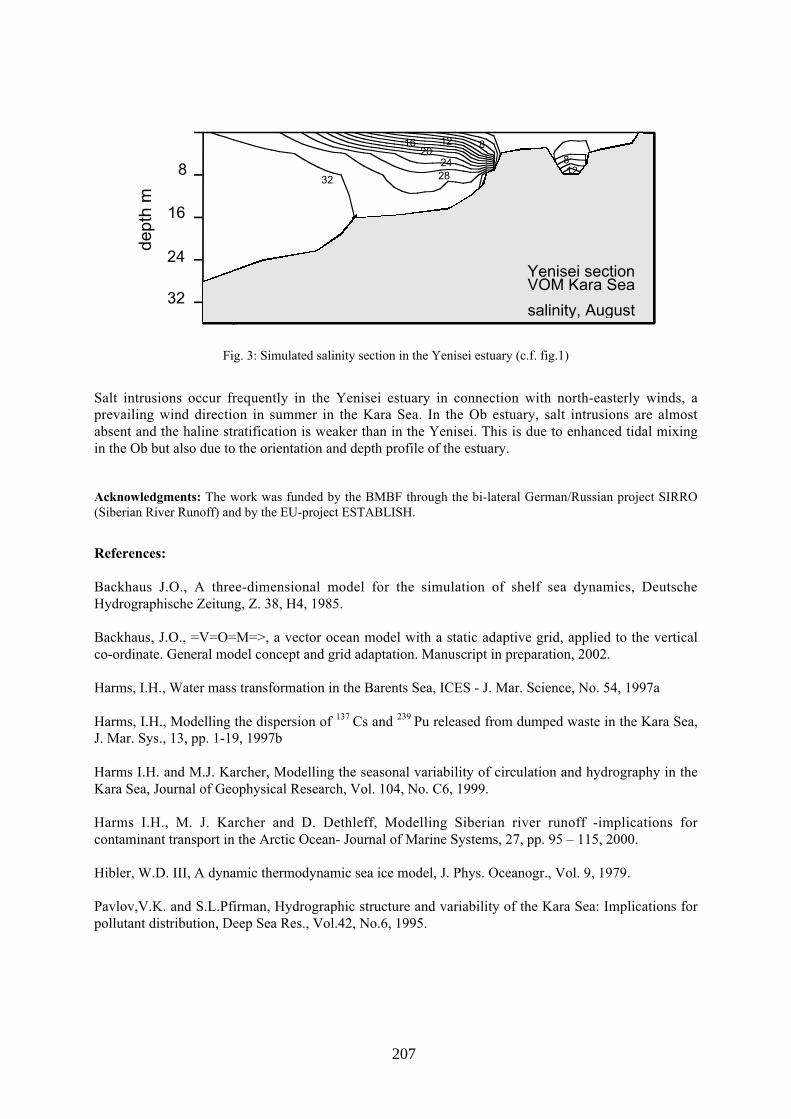
207

Fig. 3: Simulated salinity section in the Yenisei estuary (c.f. fig.1)

Salt intrusions occur frequently in the Yenisei estuary in connection with north-easterly winds, aprevailing wind direction in summer in the Kara Sea. In the Ob estuary, salt intrusions are almostabsent and the haline stratification is weaker than in the Yenisei. This is due to enhanced tidal mixingin the Ob but also due to the orientation and depth profile of the estuary.

Acknowledgments: The work was funded by the BMBF through the bi-lateral German/Russian project SIRRO(Siberian River Runoff) and by the EU-project ESTABLISH.

References:

Backhaus J.O., A three-dimensional model for the simulation of shelf sea dynamics, DeutscheHydrographische Zeitung, Z. 38, H4, 1985.

Backhaus, J.O., =V=O=M=>, a vector ocean model with a static adaptive grid, applied to the verticalco-ordinate. General model concept and grid adaptation. Manuscript in preparation, 2002.

Harms, I.H., Water mass transformation in the Barents Sea, ICES - J. Mar. Science, No. 54, 1997a

Harms, I.H., Modelling the dispersion of 137 Cs and 239 Pu released from dumped waste in the Kara Sea,J. Mar. Sys., 13, pp. 1-19, 1997b

Harms I.H. and M.J. Karcher, Modelling the seasonal variability of circulation and hydrography in theKara Sea, Journal of Geophysical Research, Vol. 104, No. C6, 1999.

Harms I.H., M. J. Karcher and D. Dethleff, Modelling Siberian river runoff -implications forcontaminant transport in the Arctic Ocean- Journal of Marine Systems, 27, pp. 95 � 115, 2000.

Hibler, W.D. III, A dynamic thermodynamic sea ice model, J. Phys. Oceanogr., Vol. 9, 1979.

Pavlov,V.K. and S.L.Pfirman, Hydrographic structure and variability of the Kara Sea: Implications forpollutant distribution, Deep Sea Res., Vol.42, No.6, 1995.

dept

h m

8

16

24

32

Yenisei sectionVOM Kara Sea

salinity, August

32 2824

2016 12 8

812

208

Lateral variability in a shallow, wind-driven estuaryJANELLE V. REYNOLDS-FLEMING

(Institute of Marine Sciences, 3431 Arendell St., Morehead City, NC 28557,[email protected])

RICHARD A. LUETTICH, JR.

(Institute of Marine Sciences, 3431 Arendell St., Morehead City, NC 28557,[email protected])

1. IntroductionThe study of lateral variability in estuarine waters is receiving greater attention since the initial studiesof typial estuarine circulation which assumed lateral uniformity (Pritchard, 1956). The interactionsbetween freshwater discharge, tidal and wind forcing and estuarine bathymetry can have profoundeffects on the lateral distribution of salinity, sediments and nutrients. Schroeder (1978) noted lateralvariability in bottom salinity in Mobile Bay and related it to freshwater discharge rates. He also notedthat winds played a role in the recorded variability. Wong and Moses-Hall (1998) completed acomprehensive study of the transverse salinity distribution at tidal and subtidal time scales in theDelaware Bay. Tidal variability was due to the interaction between tidal flows and variations in thebathymetry whereas subtidal variability was controlled primarily by local atmospheric forcing andsecondarily by discharge.

Lateral variation can have significant effects on the distribution of nutrients, oxygen, and biomass.Malone et al. (1986) recorded tilts in the pycnocline along the main axis of the Chesapeake Bay thatexplained lateral variations in phytoplankton biomass, production and dissolved oxygen. Sanford et al.(1990) also recorded these tilts in the pycnocline in the upper Chesapeake Bay and attributed them tothe local wind regime advecting saline, hypoxic water from below the pycnocline onto the flanks ofthe Bay and into the lower reaches of adjoining estuaries.

The Neuse River Estuary (NRE), located in North Carolina, USA, is a shallow, partially stratified,eutrophic, freshwater and wind-driven estuary whose density is mainly determined by salinity(Luettich et al. 2000). We document the lateral variability in salinity, circulation, and dissolvedoxygen for a range of frequencies and show how freshwater discharge and local atmospheric forcingcontrol this variability.

2. Methods

Field data

Two bottom-mounted, upward facing ADCPs were installed near the north and south shores of theNRE, approximately 32km downstream from the head of the estuary (figure 1). These ADCPsrecorded flow data in 20cm depth bins every 3min semi-continuously from June 13, 1999 toSeptember 27, 2000. Attached to each ADCP stand was a SeaBird Microcat 37-SM, which recordedconductivity, temperature and depth at a fixed point near the bottom. Approximately 25m shorewardof the ADCPs were deployed two vertically profiling platforms (profilers). The profilers lowered andraised a Hydrolab datasonde 4a with attached DO sensor through the water column every 15min(Reynolds-Fleming et al, 2002). The profilers were deployed for 30 consecutive days beginning June24, 2000. Quarter hour near surface and near bottom salinity and DO was measured by the USGS atstations upstream of the ADCP (figure 1).

209

Hourly wind direction and speedand air temperature were collectedfrom the Cherry Point MarineCorps Air Stations (CPMCAS) anddistributed by the State ClimateOffice of North Carolina. Thealong and across channel winddirections are defined oncoherence studies between wind,salinity and water level (Reynolds-Fleming and Luettich, submitted).

Figure 1. The Neuse River Estuary study site.

Model data

The hydrodynamics of the NRE were simulated using the mechanistic, three-dimensional, finite-difference model, Environmental Fluid Dynamics Code (EFDC). The EFDC model solves the three-dimensional, hydrostatic, free surface, turbulent averaged equations of motion for a variable densityfluid. The model uses a stretched or sigma vertical coordinate system and Cartesian or curvilinear,orthogonal horizontal coordinate system. Dynamically coupled transport equations for turbulentkinetic energy, turbulent length scale, salinity and temperature are also solved (Hamrick, 1992).

Figure 2. Bottom salinity along the shores from modeland field data from summer 2000

Figure 3. Across channel wind speed and the LateralSalinity Index ILSI) of both field and model data.

210

The model was calibrated with 1998 water qualitydata collected as part of the MODMON(MODeling and MONitoring of the Neuse RiverEstuaryhttp://www.marine.unc.edu/neuse/modmon.html)program (Luettich et al, 2000). Boundaryconditions included freshwater discharge,atmospheric inputs like wind and solar radiation,and water level and salinity information at theopen boundary located at the mouth of the estuary.We independently validated the model with thedata collected during our field deployments andused the model to determine the physicssurrounding fish kills that occurred duringSeptember, 2000.

3. ResultsThe validated EFDC model was able to captureapproximately 80% of the natural variability ofnear bottom salinity in the NRE. During a twentyday period of the summer of 2000, the modelreplicated diurnal and lower frequency variability.At periods of 2-4 days, the wind regime controlledlateral variability in bottom salinity evident in30hr low-pass filtered bottom salinity from both

Figure 4. Simulated upwelling conditions duringSeptember 2000 (LSI> 0 implies upwelling along the

N shore and LSI<0 implies upwelling along the Sshore).

the field and model data (figure 2 d and e). Specifically, winds blowing towards the NE caused lesssalty water to be downwelled along the north shore reducing bottom salinity. Concurrently, bottomsalinity along the south shore increased. As winds blew towards the SW, the situation reversed andsaltier water was upwelled along the north shore and fresher water was downwelled along the southshore. The unfiltered bottom salinity data showed higher frequency variability due to variations inwind speed. Here, winds often reduced in speed during the evening allowing the water column toequilibrate as bottom salinities adjusted to pre-upwelling values (figure 2 b and c).

Upwelling along the shores was quantified by defining a Lateral Salinity Index (LSI) and comparingthat to the across channel wind speed. The LSI is the difference between demeaned salinities along thenorth and south shores. If the LSI was positive, upwelling occurred along the north shore. If the LSIwas negative, upwelling occurred along the south shore. Profiler data increased the vertical resolutionof salinity data and we focused our analysis on the near surface middle, and near bottom depths. Themodel replicated upwelling conditions (figure 3). Wind blowing towards the NE, positive acrosschannel wind, led to upwelling conditions along the south shore that extended vertically to the nearsurface (figure 3). Negative across channel winds led to upwelling conditions along the north shore.Upwelling patterns were sensitive to decreases in wind speed as the nightly decrease led to a reversalin the LSI.

The EFDC model simulated salinity conditions during September 24-27, 2000 when two fish killswere reported. Wind-driven upwelling events were evident during the report and investigation of thesefish kills (figure 4). We suggest that these upwelling events, which extended through the watercolumn, were the cause of the fish kills.

References

Hamrick, J.M. 1992. A three-dimensional Environmental Fluid Dynamics Computer Code:Theoretical and Computational Aspects. Technical report, The College of William and Mary, VirginiaInstitute of Marine Sciences. Special Report 317.

211

Luettich, R.A., Jr., J.E. McNinch, H.W. Paerl, C.H. Peterson, J.T.Wells, M. Alperin, C.S. Martens,and J.L. Pinckney. 2000. Neuse River Estuary modeling and monitoring project stage 1: hydrographyand circulation, water column nutrients and productivity, sedimentary processes and benthic-pelagiccoupling, and benthic ecology. Report UNC-WRRI-2000-325B, Water Resources Research Instituteof the University of North Carolina, Raleigh, NC, 172p.

Malone, T.C., W.M. Kemp, H.W. Ducklow, W.R. Boynton, J.H. Tuttle, and R.B. Jonas. 1986. Lateralvariation in the production and fate of phytoplankton in a partially stratified estuary, MEPS, 32, 149-160.

Pritchard, D.W. 1956. The dynamic structure of a coastal plain estuary. J. Mar. Res., 15, 33-42.

Reynolds-Fleming, J.V., J.G. Fleming, and R.A. Luettich, Jr. 2002. A portable autonomous verticalprofiler for Estuarine applications. Estuaries, 24(1):142-147.

Reynolds-Fleming, J.V. and R. A. Luettich, Jr. Wind-driven lateral variability in a partially mixedestuary and its influence on fish kills. Sumbitted to Continental Shelf Research.

Sanford, L.P., K.G. Sellner, and D.L. Breitburg. 1990. Covariability of dissolved oxygen with physicalprocesses in the summertime Chesapeake Bay. J. Mar. Res., 48, 567-590.

Schroeder, W.W. 1978. Riverine influence on estuaries: A case study, in Estuarine Interactions, M.L.Wiley, Ed., Academic, San Diego, California, 347-364.

Wong, K-C and J.E. Moses-Hall. 1998. The tidal and subtidal variations in the transverse salinity andcurrent distributions across a coastal plain estuary. J. Mar. Res., 56, 489-517.

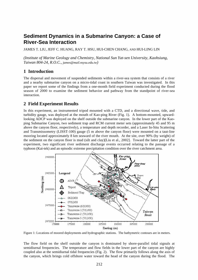
212

Sediment Dynamics in a Submarine Canyon: a Case ofRiver-Sea InteractionJAMES T. LIU, JEFF C. HUANG, RAY T. HSU, HUI-CHEN CHANG, AND HUI-LING LIN

(Institute of Marine Geology and Chemistry, National Sun Yat-sen University, Kaohsiung,Taiwan 804-24, R.O.C., [email protected])

1 IntroductionThe dispersal and movement of suspended sediments within a river-sea system that consists of a riverand a nearby submarine canyon on a micro-tidal coast in southern Taiwan was investigated. In thispaper we report some of the findings from a one-month field experiment conducted during the floodseason of 2000 to examine the sediment behavior and pathway from the standpoint of river-seainteraction.

2 Field Experiment ResultsIn this experiment, an instrumented tripod mounted with a CTD, and a directional wave, tide, andturbidity gauge, was deployed at the mouth of Kao-ping River (Fig. 1). A bottom-mounted, upward-looking ADCP was deployed on the shelf outside the submarine canyon. In the lower part of the Kao-ping Submarine Canyon, two sediment trap and RCM current meter sets (approximately 45 and 95 mabove the canyon floor, respectively), a temperature and depth recorder, and a Laser In-Situ Scatteringand Transmissometry (LISST-100) gauge (5 m above the canyon floor) were mounted on a taut-linemooring located approximately 8 km seaward of the river mouth. At the site, over 90% (by weight) ofthe sediment on the canyon floor is mud (silt and clay)[Liu et al., 2002]. Toward the latter part of theexperiment, two significant river sediment discharge events occurred relating to the passage of atyphoon (Kai-tek) and an episodic extreme precipitation condition over the river catchment area.

Figure 1: Locations of moored deployments and hydrographic stations. The bathymetric contours are in meters.

The flow field on the shelf outside the canyon is dominated by shore-parallel tidal signals atsemidiurnal frequencies. The temperature and flow fields in the lower part of the canyon are highlycoupled also at the semidiurnal tidal frequencies (Fig. 2). The flow primarily follows along the axis ofthe canyon, which brings cold offshore water toward the head of the canyon during the flood. The

213

largest size fraction captured by the two sediment traps is very fine to medium silt whereas near thecanyon floor, the suspended sediment concentration (SSC) is dominated by sand. During the passageof Typhoon Kai-tek, the increase of the wave height observed at the river mouth correlates well withthe amount of sand captured by the traps and the amount in the upper trap exceeds that in the lowertrap (Fig. 3).

Figure 2: Observed N-S component of the flow and temperature located at (a) 95 m and (b) 45 m above thecanyon floor.

Figure 3: Significant wave height observed on the tripod and the grain-size frequency distribution (GSFD) of thesand fraction of the trap sediment samples measured by a Laser Particle Analyzer (Coulter LS100).

The 'behavior' of the 32 different grain sizes in the SSC near the canyon floor observed by LISST-100can be differentiated into a coarse group (sand) and a fine group (mud) by using the empiricalorthogonal (eigen) function (EOF) analysis technique. Each group has distinct spectral characteristicsthat show major energies at subtidal (about 10 days), diurnal, and semidiurnal frequency bands. Thetheoretical ‘in-situ’ settling velocity for quartz spheres of clay, very fine silt, coarse silt, and sand sizeswere estimated based on a empirical equation [Gibbs et al., 1971], using the observed ‘in-situ’ densityfield from two cruises on June 20 and July 12, 2000. Due to the strong stratification in the canyon, thesettling of suspended sediments becomes progressively slower as they fall deeper into the canyon.Subsequently, the time needed for the four grain sizes to fall from the sea surface to the canyon floorwas estimated by dividing the water depth by the vertically averaged settling velocity. The resultsshow that the time difference for sediment grains to settle through the canyon between the sand andthe clay is on the order of hours and months (Fig. 4).

214

Figure 4: Depth-averaged settling time for the four grain sizes along the axis of the submarine canyon for thehydrographic condition surveyed on (a) June 20, and (b) July 12, 2000. The horizontal distance is relative to themost landward profiling station (zero distance).

Instantaneous suspended sediment fluxes for the above mentioned four grain-size groups at 5 m abovethe canyon floor were estimated by multiplying the total SSC measured by the LISST-100 and the N-Scomponent of the flow measured by the RCM current meter at 45 m above the canyon floor assumingthe flow field in the lower part of the canyon was spectrally coherent. Since the resulting flux showedstrong tidal signals, each of the flux time series was then decomposed into the tidal and nontidal(residual). To estimate the accumulated (net) suspended sediment transport, the instantaneous total,tidal, and residual fluxes were multiplied by the observation time interval (1 hour), and incrementedfor the entire sampling period. The results show that tidal currents were the most importantmechanism to transport suspended sediment in the lower part of the canyon whose net transportdirection was landward (Fig. 5). However, the tidal transport was modulated by the spring/neap tide(Fig. 5b). The spring tide tends to transport sediment landward and the neap tide tends to transportsediment seaward. The net nontidal sediment transport in the lower part of the canyon was zero forthe obsrevation period (Fig. 5c). Cross-spectral analyses among the SSC of 4 grain-size fractionsmeasured near the canyon floor and the SSC measured at the river mouth indicate that the sandfraction near the canyon floor has the highest correlation with the SSC at the river mouth at subtidalfrequencies, having zero time lag. Additionally, the patterns of the accumulated sediment dischargeby the river and the total SSC near the canyon floor follow each other closely during the one-monthlong deployment.

3 Concluding RemarkThese preliminary results indicate that the bottom nepheloid layer near the canyon floor consists ofclay-to-medium-silt-sized 'standing' population, which are subject to subtidal and tide-related motions.Coarser sediments such as sand and coarse to medium silt are 'drop-ins'. They are either resuspendedoff the shelf floor by the wave field or exported by the river and subsequently fall into the canyon in amatter of hours. The drop-ins are more subject to the higher frequency semidiurnal motions of thecurrents inside the canyon. They contribute to the high value of measured downward mass fluxes(exceeding 700 g m-2 day-1) in the lower part of the canyon.

References:

Gibbs, R.J., M.D. Mathews, and D.A. Link, The relationship between sphere size and settling velocity.Journal of Sedimentary Petrology, 41, 7-18, 1971.

215

Liu, J. T., K.-j. Liu, and J. C. Huan, The influence of a submarine canyon on river sediment dispersaland inner shelf sediment movements: a perspective from grain-size distributions. Marine Geology,181 (4), 357-386, 2002.

Figure 5: Cumulative hourly sediment transport of the four grain-size fractions near the canyon floor: (a) totaltransport, (b) tidal part of the transport, and (c) nontidal (residual) part of the transport.

216

The Influence of Asymmetries in Stratification on SedimentTransport in a Partially Mixed EstuaryMALCOLM SCULLY

(Virginia Institute of Marine Science, College of William & Mary, P.O. Box 1346, GloucesterPoint, VA 23062, USA, [email protected])

CARL FRIEDRICHS

(Virginia Institute of Marine Science, College of William & Mary, P.O. Box 1346, GloucesterPoint, VA 23062, USA, [email protected])

1. IntroductionIn partially mixed estuaries, the presence of an estuarine turbidity maximum (ETM) is often attributedto the convergence of near-bed estuarine circulation with seaward-directed river flow. Fine sedimentsare thought to accumulate in a relatively low energy region near the limit of saltwater intrusion. Inmany estuaries, vertically sheared tidal currents interact with the along-channel salinity gradientleading to greater salinity stratification on the ebb phase of the tide. It has been suggested that thismechanism of tidal straining will lead to increased near-bed turbulence during the flood tide andcontribute to the landward flux of salt (Simpson et al., 1990). Numerical modeling results demonstratethat asymmetries in bed stress caused by semi-diurnal changes in stratification may play an importantrole in the formation and maintenance of an ETM (Geyer, 1993; Lin and Kuo, 2001). Several datasets collected in the York River over the past six years were examined to evaluate the importance ofasymmetries in stratification to sediment transport and provide direct observational evidence for theinfluence of stratification on near-bed Reynolds stress.

2. ResultsDuring the springs of 1998 and 1999, observations were collected during 24-hour anchor stations inthe main channel of the York River estuary. During the periods of observation, tidal straining of thealong-channel salinity gradient resulted in greater density stratification during the ebb phase of thetide. Higher suspended sediment concentrations were observed during the flood tide, despite the factthat the near-bed current velocities and velocity shear were approximately equal. Net up-estuarysediment transport near the bed was observed despite the fact that tidally averaged residual near-bedcurrents were zero or slightly seaward directed (figure 1). We infer that greater salinity stratificationon the ebb reduced the intensity of near-bed turbulent mixing, limiting fine sediment resuspension.While several indirect measurements suggest higher near-bed turbulence on the flood tide, no directmeasurements were taken during the anchor stations.

In order to more conclusively link changes in stratification to near-bed turbulence and sedimenttransport, data collected during several additional experiments in the York River were examined. Ineach experiment, benthic boundary layer tripods were deployed equipped with acoustic Dopplervelocimeters (ADVs) at several heights above the bed, so that direct measurements of turbulentReynolds stress could be made. The most extensive of these experiments occurred in 2002, when S4moorings were deployed to characterize top to bottom salinity differences. The results of theseexperiments highlight the conditions under which asymmetries in stratification are important tosediment transport.

Figure 2 plots the observed current magnitude against the measured Reynolds stress for more stratifiedand less stratified conditions observed in 2002. A least squares quadratic fit of the data suggests thatfor a given velocity, the Reynolds stress for stratified conditions was approximately 25% lower thanthe less stratified conditions, despite the fact that a relatively small difference in stratification wasobserved. Consistent with previous findings, the more stratified conditions corresponded to lower

217

energy neap tidal velocities, whereas the less stratified conditions were generally found during themore energetic spring tides. Preliminary evaluation of the data suggests that historically low riverdischarge resulted in incoherent patterns of tidal straining and low suspended sediment concentrations,which appeared to be the result of advection and not local resuspension of fine sediment. As a result,significant asymmetries in sediment resuspension were not observed.

Figure 1. net landwart sediment flux due asymmetric sediment resuspension during April 1999.

In contrast, high suspended sediment concentrations were observed at a tripod deployed in thesecondary channel of the York River for 10 days during April 1996. Although no concurrentmeasurements of salinity stratification were made, observations taken shortly after the end of thetripod deployment revealed significant tidal straining, with greater stratification developing during theebb. As shown in figure 3, estimates of stratification based on the non-dimensional eddy viscosity,provide strong evidence for greater salinity stratification during the ebb. As a result, under lowconcentration conditions, estimates of Reynolds stress were significantly larger during the floodingtide, resulting in greater sediment resuspension and net up-estuary sediment flux. However, duringhigh concentration conditions, sediment induced stratification appeared to significantly damp near-bedturbulence during the flood phase of the tide and play a more dominant role than salinity stratificationin controlling near-bed Reynolds stress. For most of the deployment, the gradient Richardson numberdue to suspended sediment (Ris) during the flood tide was above the critical value of 0.25 with amedian value of 0.53. However, significantly higher velocity shear during the ebb preventedsignificant sediment induced stratification from occurring, and the Ris approached, but seldomexceeded the critical value (median = 0.10). Thus, under high concentration conditions, the impact ofsediment-induced stratification during the flood appeared to have a more dominant effect than salinitystratification, preventing preferential up-estuary sediment flux.

218

3. ConclusionsThe data presented reveal how asymmetries in stratification can influence sediment transport. It isclear from these data sets that even slight changes in salinity stratification can have an importantinfluence on the near-bed turbulent Reynolds stress. Thus, the changes in stratification due to tidalstraining can lead to asymmetric sediment resuspension and increase the landward transport ofsediment. This mechanism can effectively transport sediment up-estuary in the absence of a netresidual current. However, when an abundant supply of fine sediment is available, sediment inducedstratification can also play an important role in reducing near-bed turbulence. In the shallowersecondary channel where the near-bed velocity shear was greater during ebb, sediment inducedstratification damped turbulence on the flood and effectively reduced landward sediment flux.

Figure 2. Impact of stratification on reynolds stress from ADV 105 cmab-spring 2002

u w' '

du

dzz κ

Figure 3. Influence of salinity and sediment-induced stratification on near-bed turbulence (Spring 1996)

219

References

Geyer, W.R. 1993. The importance of suppression of turbulence by stratification on the estuarineturbidity maximum. Estuaries, 16, 113-125.

Lin, J., and Kuo, A.Y. 2001. Secondary turbidity maximum in a partially mixed microtidal estuary.Estuaries, 24, 707-720.

Simpson, J.H., Brown, J., Matthews, J.P., and Allen, G. 1990. Tidal straining, density currentsand stirring in the control of estuarine stratification. Estuaries, 13, 135-132.

220

Comparing lateral tidal dispersion with density-drivenexchange in a highly unsteady, partially mixed estuaryNEIL BANAS AND BARBARA HICKEY

(School of Oceanography, University of Washington, Box 355351, Seattle WA 98195, U.S.A.,[email protected])

1. IntroductionWillapa Bay, Washington, USA (Fig. 1) is among the largest in a system of coastal-plain estuaries inthe Pacific Northwest United States, which (with the exception of the Columbia River) have receivedscant oceanographic attention. These estuaries border an Eastern Boundary ocean, and are forced bystrong tides and strong wind-driven upwelling-downwelling fluctuations on event timescales (2-10 d).Here we uses three years of hydrographic time series and transects to examine the dominant saltbalance in Willapa Bay on subtidal and longer timescales. We find that the dynamics of flushing andoceanic exchange fluctuate between control by gravitational circulation and control by lateral tidalstirring, on both the seasonal and the event scale. We find furthermore that the salt balance isfrequently unsteady to lowest order, and that the steady-state assumption so common in analyticaltreatments of estuarine dynamics (e.g., Hansen and Rattray [1965]) seriously misrepresents the role oflateral stirring processes. We develop parameterizations which allow generalization to othermacrotidal, highly unsteady systems.

124°10' 124°00' 123°50'46°20'

46°30'

46°40'lower-water-col.moorings (8 m)

surface moorings(1 m)

main channel/transect routeColumbia

River

PugetSound

N

Str. ofJuan de Fuca

Willapa Bay

50 km

Figure 1: Willapa Bay, Washington, with a portion of the Pacific Northwest coast and North America shown forcontext. The locations of moored hydrographic and velocity observations are indicated.

The Pacific Northwest coast estuaries (again, with the exception of the Columbia River) receive weak-to-moderate river input, which peaks during winter storms and is negligible during late summer.Riverflow typically varies by a hundred-fold between these seasonal extremes (in Willapa, from 10 to1000 m3 s-1). At the same time, tides on this coast are large (the mean diurnal range at the mouth ofWillapa Bay is 2.7 m) and the estuaries tend to have extensive open intertidal areas (~50% surfacearea), so tidal prisms are in general 30-50% of total estuary volume (Hickey and Banas [2002]).Flushing and adjustment times are therefore relatively short: changes in ocean salinity take ~5 d toreach the head of Willapa Bay, 40 km from the mouth. Oceanic water properties show strongvariability on the same timescale, driven by changes in the direction of the prevailing winds.Northerly, fair-weather winds produce upwelling of salty, nutrient-rich water, while southerly, foul-weather winds produce downwelling, lower salinities, and a depletion of nutrients in surface waters.Significantly, upwelling and not river input is the dominant source of nutrients for these estuaries(Roegner et al. [2002]). Thus the dynamics of bulk ocean-estuary exchange considered here (rather

221

than the dynamics of stratification and vertical mixing) form the prime physical control on estuarineecology.

2. Riverflow and gravitational circulationIn winter and spring, when riverflow in Willapa is intermittent but high, evidence of an unsteadygravitational circulation can be seen in salinity and velocity time series. Residual, upstream velocitiesin the lower layer of the main channel show a linearly correlation with along-channel density gradient,and their magnitude is consistent with a simple balance between the baroclinic pressure gradient andvertical mixing, as in the canonical Hansen and Rattray theory [1965]. This density-driven flow,however, is superimposed upon spatially varying tidal residuals of similar or greater magnitude, whichfrequently oppose it (Hickey et al. [2002]).

Stratification appears to oscillate between two dynamical limits (Fig. 2). In the upper limit,stratification follows the 2/3-power-law relationship with riverflow which indicates an gravitationalcirculation in balance with flushing of salt by net river outflow (Monismith et al. [2002], others). InFig. 2 a solid line marks this theoretical curve, and dashed lines mark 95% confidence limits on theconstant of proportionality. This constant is determined empirically by regessing riverflow andbaroclinic velocity to the along-channel salinity gradient.

In the lower stratification limit, intrusions of a strong, buoyant plume from the Columbia River, 50 kmsouth, eliminate stratification and flatten the along-channel gradient for days or weeks at a time. Theseeffects, which occur under downwelling conditions that bring the Columbia plume north and onshore,undermine density-driven exchange even when local riverflow is substantial. Thus the unsteadiness ofthe gravitational circulation is a result not just of unsteady river input, but more important, large andrapid fluctuations in ocean salinity. During a transition between plume-intrusion and upwellingconditions, salinity at the mouth can change several psu over one or two tidal cycles.

Riverflow (m3 s-1)

8

6

4

2

010 100 1000

Bay Center

∂s/∂x large( > 0.2 psu/km)

intermediate

∂s/∂x < 0(fresher seaward:Columbia R. intrusion)

no mooring data

min

mea

nm

ax

riverflow overpast 5 d

Ver

tical

sal

inity

diff

eren

ce (

psu)

grav

itatio

nal c

irc.

bala

nces

river

flus

hing

Figure 2: Relationship between stratification and riverflow at Bay Center, 18 km from the mouth. Stratificationdata is from 39 hydrographic transects over three years; these are instantaneous observations and thus tidallyaliased. For each transect, symbol shading indicates the strength of the tidally averaged along-channel salinitygradient (∂s/∂x), from mooring data.

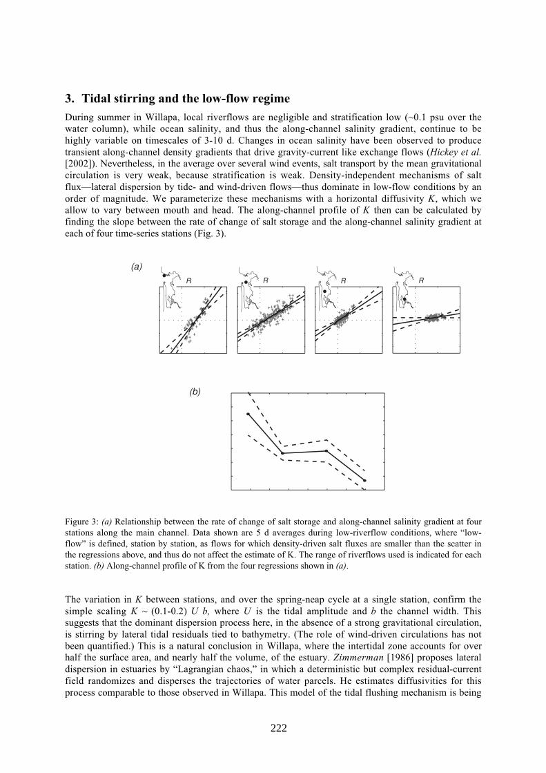
222

3. Tidal stirring and the low-flow regimeDuring summer in Willapa, local riverflows are negligible and stratification low (~0.1 psu over thewater column), while ocean salinity, and thus the along-channel salinity gradient, continue to behighly variable on timescales of 3-10 d. Changes in ocean salinity have been observed to producetransient along-channel density gradients that drive gravity-current like exchange flows (Hickey et al.[2002]). Nevertheless, in the average over several wind events, salt transport by the mean gravitationalcirculation is very weak, because stratification is weak. Density-independent mechanisms of saltflux—lateral dispersion by tide- and wind-driven flows—thus dominate in low-flow conditions by anorder of magnitude. We parameterize these mechanisms with a horizontal diffusivity K, which weallow to vary between mouth and head. The along-channel profile of K then can be calculated byfinding the slope between the rate of change of salt storage and the along-channel salinity gradient ateach of four time-series stations (Fig. 3).

Along-channel salinity gradient (psu km-1)

Rate of changeof upstreamsalt storage(psu cm s-1)

-0.2 0 0.2 0.4

-20

0

20

-0.2 0 0.2 0.4 -0.2 0 0.2 0.4-0.2 0 0.2 0.4

(a)Riverflow

R < 80 m3 s-1 R < 40 m3 s-1 R < 20 m3 s-1 R < 10 m3 s-1

0

400

800

1200

0 10 20 30 40Distance from mouth (km)

Diffusivity K(m2 s-1)

(b)

Figure 3: (a) Relationship between the rate of change of salt storage and along-channel salinity gradient at fourstations along the main channel. Data shown are 5 d averages during low-riverflow conditions, where “low-flow” is defined, station by station, as flows for which density-driven salt fluxes are smaller than the scatter inthe regressions above, and thus do not affect the estimate of K. The range of riverflows used is indicated for eachstation. (b) Along-channel profile of K from the four regressions shown in (a).

The variation in K between stations, and over the spring-neap cycle at a single station, confirm thesimple scaling K ~ (0.1-0.2) U b, where U is the tidal amplitude and b the channel width. Thissuggests that the dominant dispersion process here, in the absence of a strong gravitational circulation,is stirring by lateral tidal residuals tied to bathymetry. (The role of wind-driven circulations has notbeen quantified.) This is a natural conclusion in Willapa, where the intertidal zone accounts for overhalf the surface area, and nearly half the volume, of the estuary. Zimmerman [1986] proposes lateraldispersion in estuaries by “Lagrangian chaos,” in which a deterministic but complex residual-currentfield randomizes and disperses the trajectories of water parcels. He estimates diffusivities for thisprocess comparable to those observed in Willapa. This model of the tidal flushing mechanism is being

223

tested against results from a spatially explicit numerical model of Willapa, a version of ECOM-si, inwhich wetting and drying of the intertidal zone is resolved.

Flushing by tidal dispersion yields an inherently unsteady salt balance: that is, upstream diffusion ofsalt is balanced by a net change in salt storage rather than a downstream salt flux. Indeed, thedownstream advection of salt by the mean riverflow ("river-flushing") is negligible in Willapa duringlow-flow, summer conditions. Significantly, however, even in very low-flow conditions the upperlimit on stratification described above, the balance between gravitational circulation and river-flushing, continues to hold. A baroclinic feedback mechanism between riverflow and stratification(such as that described by MacCready [1999]) appears to be in effect, even when the overall saltbalance of the estuary is controlled by other mechanisms.

4. Tide-controlled and density-controlled regimesOn the basis of 1) the along-channel profile of tidal diffusivity K and 2) the observed slope betweenthe along-channel salinity gradient and baroclinic velocity, at each point along-channel we can definea critical stratification, above which salt transport by gravitational circulation exceeds that by tidaldiffusion, and below which tidal diffusion dominates. In the seaward reach of the estuary this criticallevel is very high—a vertical salinity variation of 3-7 psu—so that tidal diffusion dominates during allbut the largest storm events. At the head of the estuary, the critical stratification is much lower (~0.6psu), and gravitational circulation dominates during all but the lowest flows of the year. The limitingrelationship between stratification and riverflow described above allows us to rewrite this criticalstratification as a critical riverflow. Thus this method provides a set of parameters that let us predictthe dynamical balance in Willapa from its forcing alone, rather than from its hydrographic response,and without imposing the unrealistic assumption of a steady state. The method is general andpresumably applicable to any estuary in which tidal and freshwater forcing compete closely.

Acknowledgments: This work was supported by the Pacific Northwest Coastal Ecosystems Regional Study(PNCERS) and Washington Sea Grant. Many thanks to Dr. Jan Newton and the Washington State Dept. ofEcology, who generously provided much of the data used in this analysis.

References:

Hickey, B.M. and N.S. Banas. 2002. Oceanography of the Pacific Northwest coastal ocean andestuaries with application to coastal ecosystems. Estuaries. Submitted.

Hickey, B.M., M. Zhang, and N. Banas. 2002. Coupling between the California Current System and acoastal plain estuary in low riverflow conditions. J Geophys. Res. In press.

MacCready, P. 1999. Estuarine adjustment to changes in river flow and tidal mixing. J. Phys.Oceanogr. 29: 708-726.

Monismith, S.G., W. Kimmerer, J.R. Burau, and M.T. Stacey. 2002. Structure and flow-inducedvariability of the subtidal salinity field in northern San Francisco Bay. J. Phys Oceanogr. In press.

Roegner, G.C., B.M. Hickey, J.A. Newton, A.L. Shanks, and D.A. Armstrong. 2002. Estuarine-nearshore links during a coastal upwelling-downwelling cycle: plume and bloom intrusions intoWillapa Bay, Washington. Limnol. and Oceanogr. In press.

Zimmerman, J.T.F. 1986. The tidal whirlpool: A review of horizontal dispersion by tidal and residualcurrents. Neth. J. Sea Res. 20: 133-154.

Fluxes of salt and suspended sediments in a curving estuary

Jack Blanton�and Harvey Seim

�

�� Skidaway Institute of Oceanography� �� Ocean Science Circle� Savannah� GA�� USA� email� jackskio�peachnet�edu

�� Department of Marine Science� University of North Carolina at Chapel Hill�CB �� Venable Hall� Chapel Hill� NC � �� USA�email� harvey seimunc�edu

� Introduction

This study focuses on the transport of salinity and suspended sediments in a curvingchannel of the Satilla River estuary� a mesotidal estuary located in the southeastern U�S�

We examine a month�long data set to describe the circulation and �ux of salt and sediment

over a limited reach that includes a sharp channel bend� We describe the low frequency

changes in salinity� currents and optical backscatterance in the study area� Observations

were obtained during a period of steadily decreasing river discharge that represents a

period when transport of sediments to the ocean was negligible�

� Observations

Spatial changes in secondary circulation has an e�ect on the along�channel �ow ��Seim

et al�� at the landward and seaward ends of the curving channel� During spring�

�ood currents were consistently stronger at the landward end while ebb currents were

consistently stronger at the seaward end� This is attributed to the addition of momentum

to bottom currents by the cross�axis secondary circulation acting throughout the channel

bend �Seim and Gregg� �� Therefore� strong �ood currents at spring tide would cause

bottom stress to increase in the landward direction along the channel bend� and thereby

account for signi cantly higher optical backscatterance observed at the landward station

during spring tide�

Average current pro les measured half�way between the ends of the curving channelshow export below mean low water �MLW and import in the intertidal zone above MLW�

The change to landward �ow in the intertidal zone is consistent with tidally driven residual

�ow �Ianniello� �� There were pronounced di�erences in bottom current direction at

the landward and seaward end of the curving channel� Bottom currents at the seaward

end varied greatly between neap and spring tide� showing import during neap and export

�

during spring� The di�erences at the landward end were more of a degree � strong import

at neap and weaker import at spring�

Curves representing cumulative salt �uxes at the bottom were calculated for both

ends of the channel� Fluxes were landward and approximately equal throughout neap andapproaching spring tide� This suggests that the channel was neither accumulating nor

exporting a signi cant amount of salt along the bottom� At the approach of spring tide�

cumulative �ux at the landward end decreased slightly� but cumulative �ux at the seaward

end increased steadily until it became seaward� suggesting that bottom salt content in the

channel decreased� From spring to the next neap tide� the curves become parallel only to

diverge once again as the next spring tide approached�

Cumulative sediment �uxes at the landward and seaward sites indicated a net landward

�ux of suspended sediment� Throughout the period� there was more bottom �ux during

�ood than during ebb� particularly at the landward site� substantiating the higher bottom

stress during �ood as described above� At the approach of spring tide� sediment �ux at the

landward site increased suddenly during �ood tide� Since a similar increase was absent

at the seaward end� suspended sediments were apparently evacuated along the thalwegsomewhere between the landward and seaward ends of the channel�

� Discussion

Weaker mixing at neap tide allows a clear gravitational mode to occur� with seaward �ow

above the middle of the water column and landward �ow below� As spring tide approaches�

an increase in strength of tidal pumping drives mass landward on the shallow �anks which

requires seaward �ow in the deep channel to balance the mass �Li et al�� It wouldappear that the increased tidal �ux at spring tide was su�cient to completely shut down

the gravitational mode at the bottom at the seaward end of the study domain�

In order to maintain a salt balance in the presence of divergence along the bottom�

tidal pumping must transfer salt vertically and laterally into the intertidal zone in order

to maintain the landward �ux of salt� Subtidal variations in bottom salt �ux suggest a

similar role for tidal pumping� However� tidal pumping cannot be as e�ective for sediments

as for salt since sediments are not mixed as e�ectively upward into the water column�

We use a cartoon to visualize the observed fortnightly variations of the residual cir�

culation in a channel bend �Fig� �� We invoke conservation of volume transport in any

given cross�section to complete the picture� Secondary circulation in a channel bend in�

teracts with gravitational circulation and tidal pumping� Secondary circulation actingthroughout channel bends overturn the water column as it travels around the bend �Seim

and Gregg� �� During �ood� secondary circulation adds momentum to the bottom

current in the landward direction� while that of the ebb current adds momentum to the

bottom current in the seaward direction� Secondary circulation at neap tide is too weak

to interfere with the gravitational circulation mode� A well�developed gravitational mode

at neap is illustrated by relatively strong bottom landward �ow going through the deep

�

part of the channel �Fig� �� This �ow decreases in strength with distance from bottom

and changes to seaward at the top of the intertidal zone� Within the intertidal zone� the

�ow is weakly landward due to tidal pumping� In order to achieve a neap�tide balance in a

given cross�section� we infer a relatively strong seaward �ow in shallow areas below meanlow water to compensate for the predominantly landward �ow over the deep channel�

Tidally-averaged flow on bend

b. Spring

upstream

downstream

Intertidal Region(bigger at spring)

.

Intertidal Region

a. Neap

upstream

downstream

measured near bottom flowhypothetical bottom flow

Figure �� Tidally averaged �ow on a channel bend� Neap Tide �top� Spring Tide �bottom

At spring tide when tidal pumping is maximized� there is strong landward �ow in

the intertidal zone which is compensated by a seaward bottom �ow that extends to mid�

water levels in the deeper parts of the channel� However� as distance landward increases�

the seaward bottom �ow observed at the downstream end becomes weaker� eventually

�

stalls out� and nally reverses the seaward �ow due to tidal pumping to landward �ow�

As a result� bottom stress from spring tide �ood currents increases from downstream to

upstream and accounts for signi cantly higher values of optical backscatterance observed

during spring tide at the landward end of the channel bend�Assuming our inferences are qualitatively correct� the neap near�bottom landward �ow

in the thalweg is more or less continuous throughout the axial extent of the channel and

implies the presence of a seaward �ow below MLW in the shallow areas� The spring�tide

residual �ow� however� has a gyre�like pattern �Fig� �� The seaward �ow in the straight

part of the thalweg is replaced by landward �ow in the bending thalweg� We speculate that

the switch�over occurs somewhere in the zone of maximum curvature of the bend� To close

this �ow pattern� the bottom �ow along the thalweg is compensated by seaward �ow in

the shallow areas thereby producing a counterclockwise gyre landward of the �switch�over

point� and an clockwise gyre seaward of the point�

Our observations suggest the presence of a complex re�circulation of suspended sedi�

ments� driven by secondary circulation� that exists in curving channels and that compli�

cates the traditional picture of a net landward transport of sediments� Large expanses ofintertidal zones �marshes and mud �ats common to many estuaries play an important role

in the transport of salt and sediments observed over the spring�neap cycle� The di�culty

in obtaining measurements in estuarine intertidal zones makes the quanti cation of this

role di�cult�

References

Ianniello� J� P� �� Tidally induced residual currents in estauries of constant breadthand depth� Journal of Marine Research� ��

Li� C�� Valle�Levinson� A�� Wong� K� C�� and Lwiza� K� M� �� Separating baroclinic

�ow from tidally induced �ow in estuaries� Journal of Geophysical Research� ��

��

Seim� H�� Blanton� J�� and Gross� T� �� Direct stress measurements in a shallow

sinuous estuary� Continental Shelf Research� in press�

Seim� H� and Gregg� M� �� The importance of aspiration and channel curvature in

producing strong vertical mixing over a sill� Journal of Geophysical Research� ��

��

�

228

Some aspects of the water quality modelling in the Ria deAveiro lagoon, PortugalANA CRISTINA CARDOSO

(Universidade de Aveiro, 3810 Aveiro Portugal, [email protected])

JOSÉ FORTES LOPES

(CESAM, Departamento de Física, Universidade de Aveiro, 3810 Aveiro Portugal,[email protected])

JOANA MATZEN SILVA

(Departamento de Física, Universidade de Aveiro, 3810 Aveiro Portugal)

JOAO MIGUEL DIAS

(CESAM, Departamento de Física, Universidade de Aveiro, 3810 Aveiro Portugal,[email protected])

1. IntroductionRia de Aveiro is a well mixed shallow water lagoon, situated in the Northwest coast of Portugal (40º38� N, 8º 44�W), connected to the Atlantic ocean by an artificial bar, known as Barra de Aveiro, with asurface area of about 83 km2, in high tide and 66 km2, in low tide. Two major rivers, Antuã andVouga, situated at the eastern side of the lagoon, with mean flows of 5m3/s and 50m3/s, respectivelyconstitute the main freshwater input to the lagoon. In very rainy situations the freshwater input, fromVouga�s river, may reach 820m3/s (Dias et al., [1999]).

A long network of channels composes the lagoon, with four main branches radiating from theentrance: Mira, S. Jacinto, Espinheiro and Ilhavo channels (Dias, [2001]).

The tides at the mouth of the lagoon are predominantly semidiurnal, with a mean tidal range of about2,0 m. Minimum and maximum tidal range are respectively 0,6 and 3,2m. The current speed hasmaximum values close to the lagoon mouth (1-2m/s) and decrease toward the end of the channels dueto the bottom stress at the shallow areas.

The average depth of the lagoon is around 1 m, reaching 8m in the navigation channels that arefrequently dredged.

The water quality of Ria de Aveiro results from a complex balance between pollutant emissions fromnatural and anthropogenic origin and its water auto-depuration capacity. The main anthropogenicsources of pollution are domestic and industrial discharges flows, as well as, contaminated waterinfiltration of agricultural and cattle raising activities. The seaweed catches abandon andmicrobiological pollution from domestic wastewater discharges (nutrient excess) also contribute to theorganic and chemical contamination.

2. The Numerical ModelThis work has the purpose to study the water quality in Ria de Aveiro lagoon, with the help of a two-dimensional numeric system model (Mike21, [1998]).

2.1 The water quality model

The water quality model solves the system of differential equations describing the chemical andbiological evolution of coastal waters. The state variables of the model are the following: dissolved

229

BOD (BODd), suspended BOD (BODs), sedimentated BOD (BODb), ammonia (NH3), nitrite (NO2),nitrate (NO3), Phosphorus (PO4), dissolved oxygen (DO), chlorophyll-a (CHL), faecal coliforms (CF)and total coliforms (CT). The spacial and temporal evolutions of those variables are influenced byexternal factors, such as incident solar radiation (coliform bacteria decay), discharges, bottom andsurface stresses, etc.

� Oxygen processes (O2)

A number of chemical and biologic processes affect the oxygen concentration. The main processesrelated to the dissolved oxygen are described by the follow differential equation:

dDO

dtk C DOs= + −( )2 20

33 .. −− Tddd BODk θ 20

33 .. −− Tsss BODk θ

2033 .. −− T

bbb BODk θ 204341 ... −− TNHkY θ

reaeration (1) dissolvedBOD(2) suspendedBOD(3) sedimentedBOD (4) nitrification (5)

20

5252... −− TNOkY θ ),(.. 20

11 PNFR T−− θ 2022 . −− TR θ ),(. PNFP+

DOSODHS

DOSOD

−−

_.

nitrification (6) respiration (7) and (8) photosynthesis (9) sedimented oxygen

demand (10)

Where k2 is a parameter dependent on the wind speed and flow velocities, C s is a function oftemperature and salinity, kd3, ks3, kb3 are degradation constants for BODd, BODs and BODb respectively,at 20ºC (1/day), k4 is the nitrification rate at 20ºC, k5 is the specific rate for conversion of nitrite tonitrate at 20ºC (1/day), Y 1 and Y 2 are yield factors describing the amount of oxygen used atnitrification, R1 and R2 are respectively the autotrophic and heterotrophic respiration (mg O2/l/day), θis the Arrenius temperature, T is the temperature, P is the actual production (mgO2/l/day) and F(N,P)is a limitation function by the potential nutrient limitation on photosynthesis.

A first order differential time equation for each one of the following state variables are also applied:

� Biological oxygen demand process (BOD)

The decay of different fractions of organic matter is derived from the descriptions of oxygen balance.The total BOD budgets include organic matter processes: dissolved organic matter process, suspendedorganic matter process and sedimentated organic matter process. Each one of these singular processes,which correspond to a first order differential equation, includes: BOD decay, resuspension andsedimentation.

� Ammonia (NH3), Nitrite (NO2) and Nitrate (NO3) processes

The ammonium/ammonia process includes the balance of: BODd decay, nitrification and uptake byplants, as well as, by bacteria and heterotrophic respiration.

Nitrite process and nitrate process includes nitrification and denitrification.

� Chlorophyll-a process (CHL)

The production of chlorophyll-a includes carbon and oxygen production, as well as death and settlingof chlorophyll-a.

� Temperature processes (T)

The temperature mode includes an exchange rate to account for the net surface heat transfer onair/water interface.

230

� Bacterial processes (CT , CF)

The spreading and fate of total coliforms (CT) and faecal coliforms (CF) includes the die-off of bacteriadependent of the light conditions in the water column.

2.2 The hydrodynamic and transport model

The water quality model is coupled to a hydrodynamic depth integrated model for mass andmomentum, for shallow domains, and simulates unsteady two-dimensional flows (water levels and thecurrent velocities).

The water quality model is integrated in the advection-dispersion module, which describes thephysical transport processes at each grid point covering the area of interest. The integration of thissystem requires initial and boundary conditions for all the state variables.

The system solves the process equation using a rational extrapolation method in an integrated two-stepprocedure with the advection-dispersion module:

( ) ( ) ( ) SFhCy

CyhD

yx

CxhD

xvhC

yuhC

xhC

t+−

∂

∂

∂

∂+

∂

∂

∂

∂=

∂

∂+

∂

∂+

∂

∂

Here C is the component concentration, u, v are the horizontal velocities components in x and ydirections respectively, h is the water deep, Dx, and Dy are the dispersion coefficients in x and ydirections, F is de decay coefficient, S=Qs*(Cs-C) and Qs is the discharge of fonts/sinks and Cs is thecomponent concentration of discharge of fonts/sinks.

3. RESULTSFigure 1 shows temporal series for dissolved oxygen, nutrients, chlorophyll-a and bacteria, whichevolution follows the tidal cycle with a diurnal and a forth-night periodicities. In particular, concerningnutrients it is observed that the nitrite (NO2) is strongly reduced in nitrates (NO3). Nitrateconcentration increases in time towards a mean value around 0,06 mg/l. The ammonia (NH3)concentration seems to be more sensitive to the tidal cycle fluctuating, with high amplitude around amean value of 0,04 mg/l. The dissolved oxygen concentration tends to a stationary value around 9,5mg/l in agreement with observed data (Alcantara et al., [1990] and Projecto-QP0401/90 [1991]).

Figure 2 shows concentration maps of dissolved oxygen, nutrients, chlorophyll-a and bacteria.Dissolved oxygen and chlorophyll-a increase from the ocean towards the interior of the lagoon inaccordance with the observations. Nutrients, in general, have a horizontal distributioncorresponding to high concentration values close to the river's mouth and low concentrationvalues close to the ocean boundaries.

Acknowledgements: This work was support by FCT through ModelRia and Proteu projects.

References:

ALCANT ARA, F., ALMEIDA,M. and PEREIRA, M., Qualidade Microbiológica daÀgua da Ria de Aveiro, Relat6rio POLA VEIRO, Universidade de Aveiro, Portugal,1989-1990

231

DIAS, JOAO MIGUEL, Contribution to the Study of the Ria de Aveiro Hydrodinarnics,Universidade de Aveiro Portugal, pp 228,2001

DIAS, JOAO MIGUEL, LOPES, JOSE FORTES and DEKEYSER, IV AN, Hidrologicalcharacterisation of Ria de Aveiro, Portugal, in early summer, Oceanologica acta, 22 473-485, 1999

MlKE21, Water Quality Module, release 2.7, User Guide and Reference Manual, DHIsoftware, 1998

Projecto-QP0401/90, Vigilância da Qualidade da Àgua da ria de Aveiro, rel. TF-QP02/9l,1990

Fig. 1 Temporal series for simulated DO, Nutrients, Chorophyll-a and Coiform bacteria

Fig. 2 Concentration maps for simulated DO, Nutrients, Chlorophyll-a and Coliform bacteria at 17/0 1/90 at8hOOm.

232

Seasonal Variation of Flocculation on Tidal Flats,the Scheldt EstuaryMARGARET S. CHEN

(Department of Analytical and Environmental Chemistry, Free University of Brussels,Pleinlaan 2, B-1050 Brussels; Management of the Marine Ecosystem, Royal Belgian Instituteof Natural Sciences, Rue Vautier 29, B-1000 Brussels, Belgium,[email protected])

STANISLAS WARTEL

(Management of the Marine Ecosystem, Royal Belgian Institute of Natural Sciences, RueVautier 29, B-1000 Brussels; Free University of Brussels, Pleinlaan 2, B-1050, Brussels,Belgium [email protected])

1. IntroductionFlocculated fine-grained sediment transport in estuarine intertidal areas is a highly dynamic processstrongly depending on the physical properties of suspended matter. As flocculation modifies thetexture of suspended matter (SM), it thus affects its deposition. The hydrodynamic properties ofcohesive sediment flocs in tidal waters and the resulting sediment transport depend on the strength ofthe flocs (see Kranenbrug [1999]). However, little is known about the true texture of SM, since thesize of particles in suspension has been conventionally determined by granulometric analysis afterdestruction of inter-particle bindings. This study reviews a one-year biweekly measurement of SM onboth freshwater and brackish water tidal flats in the Scheldt estuary. It evaluates the seasonal variationof sediment properties, organic matter (OM) content, and flocculation status of SM in the tidal water.The flocculation status includes floc’s shape, sphericity and microfabric, which properties are believedto be significant in the sedimentary processes on the tidal flats.

2. MethodsSM was collected biweekly in siphon samplers for a one-year period (September 2000 – September2001) from two tidal flats in the Scheldt, a freshwater tidal flat (FTF) and a brackish water tidal flat(BTF, with a yearly salinity range from 5 to 27). Short-term sedimentation rate was measured using asediment trap which is a disc-shaped plastic dish (diameter of 23.3 cm and 4 mm in height) attached tothe surface of the tidal flat. Every 14 days after a spring-neap cycle, the sediment trap was collected atneap tide and replaced. The dry weight of the deposited SM was determined in the laboratory.Sediment properties of SM were determined using a method described in Wartel et al. [1995], and thegrain size distribution of the fine fraction (< 75 µm) was obtained using the Sedigraph 5100. Analysesof OM content were made using standard loss on ignition at 430°C for 24hrs method. Duplicate ortriplicate samples were taken for the floc study, and the maximum particle size that can be sampled is5000 µm due to the device’s limitation. Natural floc material was retained on 0.2 µm pore-size filterusing an experimentally tested optimal preparation procedure to acquire natural flocs that reflect the insitu state of the flocculation as closely as possible. Flocculation status was examined usingEnvironmental Scanning Electron Microscope (ESEM) under the wet mode. The ESEM wet modetechnique insures the examination of fresh wet natural sample and avoids accustomed arbitrarymodification of the sample during procedures of critical point drying and coating. For each sample aminimum of 20 images was taken and at least 400 and up to 1000 flocs were measured.

233

3. ResultsSediments in the SM are fine-grained with a clay fraction (less than 4 µm) of more than 50 % of thetotal grain-size distribution on both tidal flats. Percentage sand on the FTF is relatively higher, around10 % and up to 17 %, than on the BTF where it is about 2-3 % around the year. The mean diameter ofthe suspended sediments is below 3 µm on both tidal flats. Over this one-year period, high waterdischarge appears from November to April (winter and spring) with a maximum of 450 m3/s in March,and low water discharge is from June to August (summer) with a minimum of 40 m3/s in August.Short-term sedimentation rate is positively correlated to water discharge with average values of950 and 1650 g/m2/spring-neap cycle on the FTF and BTF respectively.

OM content is high on the BTF with an average value of 14 ± 5 %, compared to 9 ± 1 % on the FTF.OM varies generally in parallel with the change of clay content, however, a different trend is observedon the BTF in summer time, when a remarkable increase of OM appears together with a notabledecrease of the clay fraction.

The average length of the flocs varies from 30 µm to 90 µm in different seasons over the year on bothtidal flats. The average floc size is 50-70 % smaller and flocs are relatively denser during the winterand spring periods, than the considerably larger and looser flocs appear in summer. In winter andspring, sand-sized flocs (larger than 63 µm) are more abundant on the FTF (about 20 %) than on theBTF (about 4 %). It is also important to note that at least 5 % of the flocs are larger than 100 µm andreach up to 300 µm on the FTF. During the summer time, however, a remarkable phenomenon isobserved on the BTF, where sand-sized flocs increase strongly to about 50 % of the total floc-sizedistribution, and over 5 % of the flocs are larger than 350 µm reaching up to 500 µm. Besides theseasonal variations in floc’s size and microfabric, differences in floc’s shape are also presented. ESEMexaminations reveal more elongated flocs in winter and spring (November – April), while sphericalflocs are dominant during the summer period (June – August). Furthermore, it appears that, withincreasing floc size, flocs are not necessarily more elongated, but rather expand in three dimensions.

4. DiscussionKnowledge of the natural texture of SM is of primary importance to understand the sedimentaryprocesses, and is essential to assess the sedimentation rate on tidal flats. ESEM wet mode techniquehas provided unique insight in SM texture. This one-year survey reveals some noteworthyrelationships among physical aspects of the sediments, the amount of OM, the flocculation status andtheir effects on the sedimentary processes on the tidal flats.

High sand content observed on the FTF in the winter-spring period seems to indicate that high waterdischarge in the river basin brings an important sand supply to the FTF. It is also noted that therelatively high sand content on the FTF may influence floc’s size and shape because of an abrasiveeffect of the sand grains in suspension. Collisions between the heavier sand grains and the fragilelarger flocs may break up the latter ones into denser and smaller flocs. Indeed, ESEM observationspresent more relatively dense and small flocs in winter-spring time. Floc-size distribution at thisperiod also shows that flocs rather tend to be elongated. Nevertheless, sand-sized flocs still representabout 20 % and, together with the high sand supply, contribute to the high sedimentation on the FTF inthis period.

The abundance of larger than sand-sized flocs shows a parallel trend with the measured short-termsedimentation rate over this one-year period on both tidal flats. It suggests that fine-grained sedimentstransported as sand-sized flocs affect the sedimentation rate.

The changes in floc size and sphericity reveal a positive correlation with the change of OM from thewinter and spring periods to the summer time. Larger and more spherical flocs are generated duringsummer time due to the existence of high OM, which at this time of the year is more degradable thanin winter and spring. However, the increased amount of larger and more spherical flocs does not lead

234

to a high sedimentation rate in summer compared to the winter and spring periods. This implies that,although in summer OM is high favouring large floc formation on the one hand, OM decompositioncatalyses floc’s breaking up on the other. Deposition of these degradable-OM-flocs, which appear tobe very loose, probably results in a more easily erodible sedimentation layer in summer.

5. ConclusionThe ESEM study has provided important textural observations of the flocculation status of SM. Floctexture and size exhibit clear seasonal variations and positively correlated with the measured short-term sedimentation rates on the tidal flats over this one-year survey. The changes in floc size andsphericity reveal a positive correlation with the change of OM. High OM increases floc size in a three-dimensional expanded way. Fine-grained sediments transported as sand-sized flocs have an importanteffect on the short-term sedimentation rate. It is deducted here that highly concentrated and relativelydense flocs contribute to fast sedimentation during winter and spring periods resulting in a compactsediment layer, while loosely formed flocs likely lead to an easier erodible layer in summer time. Thisdeduction not only is in agreement with sedimentation measured on the tidal flats, but also matches theresults of the suspended sediment concentration measurements in the flooding water on the twoadjacent marshes for the same one-year period.

Acknowledgments: The authors sincerely thank J. Cillis for his great technical support in the ESEM work andS. Temmerman for providing the data of sediment traps. Thanks also go to F. Francken for his assistance in thefieldwork.

References:

Kranenburg, C., Effects of floc strength on viscosity and deposition of cohesive sediment suspensions,Continental Shelf Research, 19: 1665 – 1680, 1999.

Wartel, S., J. P. Barusseau and L. Cornand, Improvement of grain-size analyses using the automatedSEDIGRAPH 5100. Documents de Travail de L'I. R. Sc. N. B., 80. Institut royal des Sciencesnaturelles de Belgique. Bruxelles, Belgique. 28 pp., 1995.

��

��

��

�� !� �� !�� "��#$!�� %%&� ��'��!�� # ��

� ��

�� Æ�� Æ� �!"� �� # �� $#�� $�� % &� � �� '�� #�� (�#�� (��% &� �� # �� (��' ��$��#� ��)�� # �� # �� '�� *�� # �� +�� %

&� � �� # �� (��' �� %,�� '�� -�� #��#�� (� ��%

,�� (�� #$��#�� (�� (�� % ,�� #��#�� #��# �� .�� /�� (�� $�� )� �� #�� -�� (�� (�� %

,�� # �� .�� (�� 01 �� ( � � �� #��#�� (�� $�� (�� 21 �� (�� (�� 3��# � � ��(��' #�� %

� /�� (�� '(�� (�� ((�� (�� %

� ��

4�� 5�� ( � �� +� �� (�� % � �� 678889� �� # � �� # �� # �� (�� # ��(��' ��#% :� �� ;<= �� #��#�� %

��

&� �� ((�� $�� # �� #��#�� 678>79 ��0

��

��? �

��

��? �

��

��@ ��

��

��? ��

?�� 7"

��

��? �

��

��? �

��

��@ ��

��

��? ��

?�� ;"

�� (�� (�� (�� "�� " �� (��#� � �� A�� (�� #� � � �� #� �� )�� #� � �� (��#� �� # �� +� � �� % ,�� )�� -�� #��(�� (� ��# �� % &� �� ;� �� (�� ( � 7�� (��%

��

,�� (�� (�� (�� 6788�9"0

�� "

��?�� "

��?�� "

��

��

��

��

@ � � � ��"

�� (�� (�� (�� (�� Æ�� )� ��(��# �� (�� (�� # �� 678B;9�� # �� 678�B9� ��(��#%

��

&� �� /�� .�� (��(� �� /�� (�� 5��

� � �� .�� # *�� "�

�� ;<C �#��#�� % , � �� 3�� 0

� ��

��@ ��

�� " ��"

�� (�� *�� @ 7� ;� � � � � �� ;<

(�� (�� %,�� $�� 5�� (�� (��

�� /�� ((�� 3��0

�� "�� @ �� "

� ?

� ��

�� "�� "

�� (% �� "�� (�� ?7 � �� (��

�� (�� "�%

,�� (�� 5�� 3�� (�� % &� �� # �� (�� $��$D�� 678879"0

�� @ E��

�� "

��

�B"

�� @ E��

�� "

� ?��

;� �?

E�

;

��>"

�� @ E��

�� "

� ?��

;� �?

E�

;

��"

�� @ E��

�� "

� ? �� ?E��

�8"

�� "�� @ �� "

� ?��

B?

��

�?

��

�?

��

B�7�"

�� "�� (�� (��

(�� (�� "� # �� # �� @ �� " �� E��

��(�� $D�� Æ��% &� �� # �� ( � �� (�� ( �� #��#�� "%

� ��

�� -�� # �� ((�� #�� #��#�� (�� (�� %

,�� *�� (�� (�� (�� % ,�� (�� )� �� % ,�� (�� *�� # �� #� � �� # �� %

,�� #�� (��# �� # �� $�� (�� +�� (�� 3�� (��% ,�� $�� (�� (�� # �� # �� % &� �� % ,�� '�� -�� # � ��$�� (�� #��%

�� !�� "� �

��

:�� 70 F�� GF (�� "��" �� (�� *�� "��"�� (�� " ��#"%

��

A�� F%� .�� % H%� G�� (�� :�� :�� (( ;� $; �� 788�%

<�� H% G%� /(�� H% :%� <��#�� &%� =#�� )�� # �� (( �>�1�� 7888%

=�#�� .% H%� G�� % H%� G�� (�� $�� (( ;8�1�� 78�B%

=�� .% .%� =��I�� D% F%� G�� H% �%� =�� <% J% �� G�� <% /%� K�� (�� (�� )��% � �� !�� A�� (( 7 ��717 � ;�7887%

D�� % J%� "� �� :�� $(�� =%.%/%F%.%�%/%�K��% � A�� J��#� A�� 78B;%

/�� H% H%� L�� .% A%� � #��$% �� #��$��&�

�� ' ( � �� ))* � �� +� �� ,�� A�(��G�� 1>��1�MA� F�� G�� ((� 78>7%

239

Sediment Dynamics in Tidal Flats and Salt Marshes of theTagus Estuary, PortugalPAULA FREIRE

(Laboratório Nacional de Engenharia Civil, Av. Do Brasil, 101, 1700-066 Lisboa, Portugal,[email protected])

CÉSAR ANDRADE

(Centro e Departamento de Geologia da Faculdade de Ciências de Lisboa, Bloco C2, 5º Piso,Campo Grande, 1749-016 Lisboa, Portugal, [email protected])

1. IntroductionThe Seixal bay is located in the southern bank of the inner Tagus estuary and consists of a shallowsemi-enclosed system with extensive tidal mudflats and salt marshes (Figure 1), which formed andaccreted during the last 500 years following the formation of the Alfeite sand spit (Freire and Andrade[1999]; Freitas et al. [1999]). The local mean tidal range in spring and neap tides is 3.2 m and 1.5 m,respectively, and the maximum tidal level above chart datum (MSL=2.2 m) is 4.3 m. The sedimentforming the tidal flats and marshes in the Seixal bay is to a large extent cohesive (silty clay) withparticulate organic matter content up to 9%. Sandy sediments are concentrated preferably in the deeperchannels. The sediment dynamics inside the Seixal Bay is almost exclusively driven by tidal currents,in contrast with the exposed beach of the sand spit, which is essentially reworked by local generatedwaves.

Figure 1: Location map of the field study area and surveyed stations.

Andrade et al. [1998], Freire [1999] and Freitas et al. [1999] studied the short to medium-termevolutionary trends of the Seixal intertidal areas using map comparison and field measurement oferosion/accretion. The results of theses studies pointed out a contrasting morphological behaviourbetween the subtidal and low-intertidal areas (net erosion) and the high-intertidal and supratidal regionof flats and marshes (net vertical accretion and no appreciable surface change).

The results of two field surveys conducted to measure and describe the patterns of suspended sedimentmovement at the time scale of a tidal cycle are presented in this paper and the results discussed withinthe context of the evolutionary trends previous reported.

240

2. MethodsTwo 13 hour-long field surveys were performed in February (neap waters) and March (spring waters)1998 in two stations of the Seixal Bay (Fig. 1): station 1, positioned in the main thalweg of the Seixalchannel (CD depth of 2 m) was equipped with one acoustic current meter RCM-9 with sensors oftemperature, conductivity and turbidity; water samples were collected at regular intervals for latercalibration of the conductivity sensor; station 2 lies 2 500 meters upstream, in the southern tidal flat(CD depth of 0.4m) and the equipment deployed consisted of a Braystoke current meter; watersamples for conductivity and turbidity measurement were collected with a horizontal van Dorn-typebottle. During the surveys the local tidal level variation was monitored using a tide gauge (see Figure 1for location). The meteorological conditions were similar during both surveys and are described inFreire [1999]. Bottom sediment mapping and hydrographical surveys of the intertidal and subtidalfeatures were also performed.

The concentration of suspended sediment was determined in the laboratory following the gravimetricmethod and using Millipore 0.45µm mesh standard filters. Particle size analysis of the residualsediment in the filters was performed by laser diffraction.

3. Results and DiscussionThe results obtained in the field surveys show that the estuary is the main source for the Seixal baysediment bed load. The sand is transported mainly during the spring tide flood and is trapped into thebay, remaining in the deeper channel near the entrance. The results also reveal that there is nosignificant input of fine material in suspension from the estuary into the bay, being the local fluvialnetwork the main source of silt-clay sediment.

Inside of the bay the resuspension of bottom sediments is particularly efficient during the spring tideebb when maximum velocities (97 cms-1) are observed (Figure 2). The finer sediment fraction (meandiameter of 10 µm), which includes most of the particulate organic matter (Figure 3), remains insuspension during the low water slack period. This promotes a flood-dominated net transport towardsthe higher intertidal flats and marsh banks. On the other hand, the coarser silt particles (mean diameterof 40 µm) are preferentially exported from the tidal flats during the ebb towards the lower flats andchannels. In this way, the tidal currents promote a textural sorting of the suspended particles by sizeand the associated deposition of the finer inorganic silt fraction with the organic fraction, which hasexpression in the bottom sediment distribution.

The amount of suspended sediment transported during the tidal cycles was evaluated. The results showthat in station 2 a residual amount of 5x103 m3 of material is transported during the ebb. Consideringthe total area influenced by the tide upstream the station 2, an average erosion rate of 0.3 cmyear-1 wasfound.

These results suggest a contrasted morphological evolutionary short-term model for Seixal bay inwhich the accretion is dominant in the high-intertidal and supratidal flats while the subtidal and low-intertidal areas show an erosional tendency. The short-term evolutionary trends and rates deducedfrom the surveys are in agreement with the medium and long-term results for the Seixal bay achievedin other studies. Freitas et al. [1999], using radiometric dating, obtained a sedimentation rate for thesalt marshes of the Seixal bay of 0.7 cmyear-1. The results presented by Freire [1999], through chartcomparison methods, show that the subtidal and low intertidal flats present an erosion tendency, withan average rate of -1 to -2 cmyear-1.

241

Spring tide

0

50

100

150

200

250

300

350

08:0

010

:00

12:0

014

:00

16:0

018

:00

20:0

0

Time

Wat

er le

vel (

cm)

0

20

40

60

80

100

Vel

oci

ty (

cms-1

)

Water level Velocity (station 1) Velocity (station 2)

Spring tide

0

50

100

150

200

250

300

350

08:0

010

:00

12:0

014

:00

16:0

018

:00

20:0

0

Time

Wat

er le

vel (

cm)

0

25

50

75

100

125

150

Co

nce

ntr

atio

n o

f S

S

(mg

/l)

Water level Concentration (station 1) Concentration (station 2)

Neap tide

0

50

100

150

200

250

300

350

08:4

509

:45

10:4

511

:45

12:4

513

:45

14:4

515

:45

16:4

517

:45

18:4

519

:45

20:4

521

:45

Time

Wat

er le

vel (

cm)

0

20

40

60

80

100

Vel

oci

ty (

cms-1

)

Water level Velocity (station 1) Velocity (station 2)

Neap tide

0

50

100

150

200

250

300

350

08:4

509

:2510

:0510

:4511

:2512

:0512

:4513

:2514

:0514

:4515

:2516

:0516

:4517

:2518

:0518

:4519

:2520

:0520

:4521

:25

Time

Wat

er le

vel (

cm)

0

25

50

75

100

125

150

Co

nce

ntr

atio

n o

f S

S

(mg

/l)

Water level Concentration (station 1) Concentration (station 2)

Figure 2: Measured time series of tidal currents velocity and suspended sediment concentration at Seixal bay.

0

20

40

60

80

100

0 20 40 60 80 100 120 140

Concentration of SS (mg/l)

PO

M (

%)

0

10

20

30

40

Mea

n d

iam

eter

(µµµµ m

)

POM vs CSS MD vs CSS

Figure 3: Suspended sediment concentration (CSS) plotted against sediment mean diameter and particulateorganic matter content (POM).

The implications of the presented model for a long-term evolution of the Seixal bay are that thispattern of evolution must be interrupted by high-intensity and low frequency episodes of activity ofthe local fluvial network, that will bring important amounts of fine sediment into the system.

4. ConclusionsIn order to characterize the composition and the short-term dynamics of the sediments in Seixal Bay,two field surveys were performed. The results show a contrasted morphological evolutionary trend ofthe subtidal and low-intertidal areas versus the high-intertidal and supratidal flats: the erosionalbehaviour is dominant in the former while the salt marshes show an accretionary tendency. Theevolutionary trends and rates obtained in this study are in agreement with the medium to long-termresults achieved by Freire [1999] and Freitas et al. [1999].

242

Acknowledgments: The first author was sponsored by Fundação para a Ciência e a Tecnologia under grantBD/2767/93-RN.

References:

Andrade, C., Freitas, M.C., Bastos, A., Abrantes, A. and A. Antunes, Micro-scale morphodynamics insalt marshes of Tagus estuary. An experimental approach. Actas V Congresso Nacional de Geologia.Comum. IGM, 84 (I), C67-C70, 1998 (in Portuguese).

Freire, P., Morphogical and sedimentary evolution of estuarine banks (Tagus Estuary, Portugal), PhDDissertation, University of Lisbon, 320p., 1999 (in Portuguese).

Freire, P., and C. Andrade, Wind-induced sand transport in Tagus estuarine beaches. First results.Aquatic Ecology, 33, 225-233, 1999.

Freitas, M.C., Andrade, C., Moreno, J.C., Munhá, J.M. and M. Cachão, The sedimentary record ofrecent (last 500 years) environmental changes in the Tagus marshes, Portugal, Geologie en Mijnbouw,77: 283-293, 1999.

243

Modelling of the seasonal dynamics of the water masses,ice and radionuclide transport in the large Siberian riverestuariesVLADIMIR MADERICH, NATALYA DZIUBA, VLADIMIR KOSHEBUTSKY, MARK ZHELEZNYAK

(Institute of Mathematical Machine and System Problems, Glushkov av. 42, 03187, Kiev,Ukraine, [email protected] )

VLADIMIR VOLKOV

(Nansen International Environmental and Remote Sensing Center, 26/28, BolshayaMonetnaya Str.197101 S.-Petersburg,Russia, [email protected]

1. IntroductionThe activities of several nuclear reprocessing plants (Siberian Chemical Combine (SCC), Mining,Chemical Combine (MCC) and Mayak Production Association (Mayak)) that are placed on thewatersheds of large Siberian rivers Ob� and Yenisey may potentially cause contamination of the ArcticOcean. Therefore, use of the models is necessary to assess the influence on potential radioactivityspreading location of these sources and impact of global warming on dispersion processes in thesystem river-estuary.

In frame of EU INCO-COPERNICUS project RADARC (Johannesen et al. [2002]) a linked chain of1D river model RIVTOX and 3D model THREETOX was used to simulate impact of the previous andpotential releases from the nuclear installations in the basins of Ob� and Yenisey rivers on theradioactive contamination of the Kara Sea and Arctic Ocean.

2. Model ChainThe model chain includes 1D river net model RIVTOX and 3D estuary model THREETOX. TheTHREETOX code (Margvelashvili et al. [1997] is intended for simulation of the transport and fate ofthe radionuclides and other contaminants in the stratified waterbodies. THREETOX includes a set ofsubmodels: a hydrodynamics submodel, ice dynamics-thermodynamics submodel, suspended sedimenttransport and radionuclide transport submodels. The hydrodynamics is simulated on the basis of thethree-dimensional, time-dependent, free surface, primitive equation model. The modified κ ε−model (Burchard and Pettersen [1999]) is used. The dynamic-thermodynamic ice and snow model isbased on the Hamburg Sea-Ice Model (Stössel and Owens [1992] that was modified byimplementation of elastic-viscous-plastic rheology. Suspended sediment transport is described by theadvection-diffusion equations, taking into account fall velocities of the sediment grains. The bottomboundary condition describes sediment resuspension or settling down depending on the ratio betweenthe equilibrium and actual near bottom suspended sediment concentration. The thickness of the upperlayer of the bottom deposition is governed by the equation of the bottom deformation. The equationsof the radionuclide transport describe the concentration of the radionuclide in solute, the concentrationin the suspended sediments and the concentration in the bottom deposition. The exchanges betweenthese forms have been described as adsorption-desorption and sedimentation-resuspension processes.Adsorption and desorption of radionuclide between liquid and solid phases are described by theradionuclide exchange rates, and by the distribution coefficients.

The one-dimensional river model RIVTOX was developed at the IPMMS (Zheleznyak et al. 1992). Itsimulates the radionuclide and chemical pollution transport in networks of river channels. Sources canbe a direct release into the river or the runoff from the catchment.The hydraulics part of the RIVTOXis based on the of Saint-Venant equations. The governing equations of the sub-model of suspendedsediment and radionuclide transport model are derived from the 3-d model equations. They describe

244

advection-diffusion transport of the cross-sectional averaged concentrations of suspended sediments,toxins in solution, toxins in suspended sediments and in bottom depositions. The adsorption-desorption and diffusion contamination transfer in the systems "solution - suspended sediments" and"solution - bottom deposition" are treated also via the distribution coefficient approach.

3. Study areaThe 1D model RIVTOX of river dynamics and radionuclide transport was adapted to the Ob� riverpath from Mayak and SCC and to the Yenisey River from MCC (see Figure 1). The river network wassubdivided into a set of branches in compliance with the location of observation points and the maintributaries. The parameters of water cross-sections for observation points were used. The monthlytributary discharges values for 1949-1995 were used to simulate river hydraulics. The data on releasefrom the radionuclide sources were collected in frame of RADARC project (Johannessen et al.[2002]). The THREETOX was customised for the Ob� and Yenisey estuaries using digitisednavigational maps of estuaries. The horizontal grid resolution is 8x6 km in the Ob� and 3 km in theYenisey. The 6hr fields of wind, air temperature, precipitation, humidity and cloudiness were usedfrom NCEP reanalysis for the period 1949-1995. Daily mean discharges of rivers, suspended sedimentand radionuclide concentrations were calculated by the RIVTOX model. In the estuary mouth, thetemperature, salinity and velocity distributions and sea level computed by the Kara Sea model(Johannessen et al. [2002]) were used in the estuary model as outer boundary conditions. Thesimulations of the period 1949-1994 were carried out for the Ob� and period 1974-1994 for theYenisey.

Figure 1: Ob� and Yenisey river system. The boxes correspond to the Mayak Production Association (Mayak),Siberian Chemical Combine (SCC) and Mining, Chemical Combine (MCC).

245

Figure 2: The computed and observed concentration of 90Sr in the Musliumovo (Techa River) (a) and measuredyearly mean release of 90Sr from Mayak vs. computed flux from Ob� estuary to the Kara Sea.

Figure 3: The computed surface fields of temperature, salinity and ice thickness in the Ob� Estuary in April 1994and surface fields of temperature, salinity and near bottom distribution of suspended sediments in September1994. The temperature and salinity are compared with KAREX-94 data.

a

1950 1960 1970 1980 1990Year

1E+0

1E+1

1E+2

1E+3

1E+4

1E+5

1E+6

SR

-90

kB

q/m

3 Computations

Measurements

b

1950 1960 1970 1980 1990Year

1E+11

1E+12

1E+13

1E+14

1E+15

1E+16

Sr-

90 fl

ux B

q/ye

ar Mayak

Ob' Estuary

0 100 200

km

0

100

200

300

400

500

600

700

km

-0.5

0.5

1.5

2.5

3.5

4.5

5.5

6.5

7.5

8.5

9.5

10.5

11.5

12.5

April, 1

T, C

0 100 200

km

0

100

200

300

400

500

600

700

km

0

2

4

6

8

10

12

14

16

18

20

22April, 1

S, ppt

0 100 200

km

0

100

200

300

400

500

600

700

km

0

0.1

0.2

0.3

0.4

0.5

0.6

0.7

0.8

0.9

1

1.1

1.2

1.3

April, 1

H, m

0 100 200

km

0

100

200

300

400

500

600

700

km

-0.5

0.5

1.5

2.5

3.5

4.5

5.5

6.5

7.5

8.5

9.5

10.5

11.5

12.5

T, C

September, 6

4.8 4.5 4.8

6.76.56.

8.79.47.8

10.510.810.4

10.310.

10.210.6

3.63.6

4.04.2

5.8

4.7

0 100 200

km

0

100

200

300

400

500

600

700

km

0

2

4

6

8

10

12

14

16

18

20

22

S, ppt

September, 6

7.5 9.5 5.9

0.10.20.

0.10.10.1

0.10.10.1

0.0.1

0.10.

8.17.3

5.54.7

1.1

6.5

0 100 200

km

0

100

200

300

400

500

600

700

km

0

0.001

0.002

0.003

0.004

0.005

0.006

0.007

0.008

0.009

0.01

0.011

0.012

0.013

0.014

September, 6

Sed, kg/m3

246

4. Results and conclusionsThe model chain was validated against the available data on river discharge, suspended sediment andradionuclide concentration, temperature, salinity and ice distribution in the estuaries. In Figure 2 thecontribution of Mayak in 90Sr contamination of the Ob� river system and the Kara Sea is presented. InFigure 2a the calculations are compared with 90Sr measurements in Musliumovo (Techa River). Asseen from figure the RIVTOX model reproduces transport of radionuclide quite well. In Figure 2b thefluxes of 90Sr from Mayak and Ob� estuary mouth to the Kara Sea are given. This figure shows thatafter strong initial contamination in early 50th the sediments in the Ob� were sources for secondarycontamination of river and estuary. Around 70% released in 1949-1994 90Sr reached the estuarymouth. The Yenisey River was contaminated the same way in 70th in result of washing up ofcontaminated sediments from the islands and flood plains. The numerical results agree quite well withthe observations of the oceanographic fields. In Figure 3 the surface fields of temperature, salinity andice thickness in the Ob� Estuary in April 1994 and surface fields of temperature, salinity and nearbottom distribution of suspended sediments in September 1994 are presented. The computedtemperature and salinity agree with the survey data from KAREX-94. The computed in other run thesalt wedge in the relatively deep Yenisey Estuary is clearly visible.

The results of multi-year simulation of the water dynamics and radionuclide transport in the Ob� andYenisey rivers and estuaries showed ability of the developed model chain to reproduce a seasonaldynamics of water mass. An important role of ice cover in the seasonal dynamics of the Ob� andYenisey estuaries also was demonstrated. The developed model chain is used for assessment of theradionuclide spreading from inland sources.

Acknowledgments: This work was funded by EU INCO-COPERNICUS project RADARC (Contract ICA-CT-2000-10037) and project INTAS � 1997-31278.

References:

Burchard, H., Petersen O. Models of turbulence in the marine environment � a comparative study oftwo-equation turbulence models. J. Marine Systems, 21, 29-53, 1999.

Johannesen, O. M., Pettersson, L. H., Gao Y., Nielsen, S.P., Borghuis, S., Strand, P., Reiersen, L. O.,Bobylev, L. P.,Volkov, V., Neelov, I., Stepanov, A., Bobylev, K., Zheleznyak, M., Maderich, V.Simulation for potential radioactive spreading in the 21 century from rivers and external sources in theRussian arctic coastal zone-RADARC, in The 5th Int. Conf. on Environmental Radioactivity in theArctic & Antarctic, edited by P. Strand, T. Jølle and Å. Sand, Norway Radiation Protection Authority,Norway, 2002.

Margvelashvili, N., Maderich, V., Zheleznyak M., THREETOX - computer code to simulate three-dimensional dispersion of radionuclides in homogeneous and stratified water bodies. RadiationProtection Dosimetry, 73, 177-180, 1997.

Stössel, A., and W. B. Owens, The Hamburg Sea-Ice Model. Report No. 3, DKRZ, 65 pp., 1992.

Zheleznyak, M., Demchenko R., Khursin S., Kuzmenko Yu., Tkalich P., Vitjuk N. Mathematicalmodelling of radionuclide dispersion in the Pripyat-Dnieper aquatic system after the Chernobylaccident. The Science of the Total Environment, 112, 89-114, 1992.

247

Spring-neap variations in residual currents and bedloadtransport rates, associated with rectilinear and rotatorytidal current systemsANA PAULA TELES

(Southampton Oceanography Centre, European Way, SO14 3ZH Southampton, U.K.,[email protected])

MICHAEL COLLINS


DAVID PUGH


1. IntroductionThe Solent Estuarine System is an important estuarine system located along the south coast of theUnited Kingdom separating the Isle of Wight from the mainland (see Collins and Ansell [2000]). Thesystem comprises the well-mixed Solent channel, the partially-mixed Southampton Water estuary, andthe harbours of Portsmouth, Langstone and Chichester, together with other smaller estuaries. TheSolent channel can be divided into two sections: the East Solent, 20 km long and 5.5 km wide; and theWest Solent, 20 km long and 4 km wide, on average. Both sections contain a deep channel, withdepths (related to Chart Datum) ranging mostly from 10 to 20 m; likewise, an extensive shallow areawith depths less than 10 m, transitionally grading into the tidal flats. The East Solent entrance is wider(8 km) with depths in excess of 30 m in the narrow deep channel (1.5 km), whilst the West Solententrance is very narrow (1.5 km) and deep (up to 60 m). The two entrances are connected to theEnglish Channel; hence, they are affected by its tidal, wave and sediment dynamics regimes. These areexamined in this contribution, in relation to potential sand transport.

2. Data AnalysisData from (5) self-recording current meter locations in the West and East Solent are analysed here, interms of residual currents and sediment transport rates. Residual currents have been measured around5 m above the bed in the East Solent and 10 m above the bed in the West Solent (in water depthsranging from 11 to 20 m). Near-bed residual currents have been calculated at 1 m above the bed, basedupon the assumption of a ‘power law’ on the vertical distribution of the currents (see Dyer [1970a]).Directionally-related (resolved into north, east, south and west components) mean and net bedloadtransport rates have been computed over neap and spring tidal cycles. Bedload transport has beencalculated on the basis of the modified Hardisty equation (see Hardisty [1983]; Wang and Gao[2001]), for ‘potential’ sand (D50= 0.14 mm (median diameter)) transport. Effectively, currents in theWest Solent are rectilinear in character; those in the East Solent are rotatory, and under certainconditions influenced by wave activity. Under the influence of waves over the same region (see Gaoand Collins [1997]), the magnitude of the directionally-related (qN, qE, qS and qW) transport ratesvaries, whilst the net transport remains relatively constant. This concept is examined here, in terms ofspring-neap tidal cycles (approx. 7.5 days each) variability and in relation to rectilinear-rotatorycurrent systems.

248

0 1.5 3 km

N

1º40’W 1º20’W

50º3

0’N

50º5

0’N

50

30

30

30

20

30

30

30

30

30

30

30

50

30

2 0

30 30

2

0

20

20

2 0 20

20

30 30

2 0

3 030

2020

30

2 0

20

30

50

50

30

10

102 0

5

50

20

10

5

5

5

5

10

10

5

20

20

5

20 105

5

20

2

5

5

10

0

0

5

5

0

0

105

5

10

10

5

10

5

10

10

0

5

10

0

30

20

20

10

30 30

5

0

11

10

UK

English Channel

10ºW 5º 0º

55º

50ºN

PortsmouthHarbour

LangstoneHarbour

ChichesterHarbour

HaylingIsland

Isle of Wight

Southampton Water

West Solent

East Solent

English Channel

0

5

10

Figure 1: The Solent Estuarine System and the 5 current meter locations ( �).

3. Summary and Conclusions

Mid-depth and near-bed residual currents

In terms of the mid-depth residual currents, those associated with rectilinear tidal current systems(West Solent) are larger in magnitude, on neaps (0.095 and 0.126 ms-1) and springs (0.125 and 0.184ms-1) compared to rotatory locations (0.006 to 0.030,and 0.031 to 0.064ms-1, respectively). Directionalvariability of the residual currents between springs and neaps ranged up to 8o for the rectilinearstations and up to 74o for the rotatory stations. In converting to near-bed residual currents, thedirectional values are slightly modified (generally, around 2 to 3o) in response to resolution of thevectors (a high difference can be associated with a low residual current).

For all the stations, the rates ranged between 0.002 and 0.093 kgm-1s-1 on neaps and 0.001 and 0.135kgm-1s-1 on springs. For the rectilinear current systems, the differences between near-bed residualcurrent and net bedload transport directions ranged from 11 to 23o, on neaps and springs; for rotatory,they ranged from 21 to 145o. Hence, the direction of the net bedload transport is relatively consistentwith the direction of the near-bed residual currents for the rectilinear current systems; it is notconsistent for the rotatory currents.

Directional mean and net bedload transport rates

In all cases, the magnitude of the directionally-related mean bedload transport rates increased fromneap to spring tidal conditions. In the case of the rotatory system, the rates show high variability, withan overall 78% to 783% increase on springs (in relation to neaps); for rectilinear, from 18% to 62%but at considerably higher transport rates. In comparison, the net rates showed similar increases (45%

249

to 61%) for the rectilinear currents; for the rotatory, they ranged from 198% to 812% (in a single case,a decrease).

Comparisons undertaken between the various directional components (qN, qE, qS, and qW), with thenet rates demonstrate: (a) consistent contributions in the case of the various mean transport ratecomponents at a particular station, on both neaps and springs, for the rectilinear currents (WestSolent); and (b) highly variable contributions for each component, on neaps and springs and at thevarious stations, for the rotatory currents (East Solent).

Thus, particularly in relation to the rotatory tidal current systems, there is strong evidence ofintensification of lateral transport under spring tidal conditions cf simulated ‘stormy’ conditions (seeGao and Collins [1997]). Similarly, there are variable contributions from the directional meantransport rates, to the net transport rates, at the same stations on both neap and spring tides.

Water circulation

In terms of mid-depth and near-bed Eulerian residual currents on neaps and springs, there is evidenceof flow out of the West Solent, towards the East Solent. This is consistent with the eastward residualcalculated previously from sea level differences (see Blain [1980]), and from current metermeasurements on neap tides with high barometric pressure and northeasterly winds (see Dyer andKing [1975]). On the other hand, it is not consistent with the westward residual occurred on springtides with low barometric pressure and southwesterly winds. The southwestly residuals observed at thewestern end of the West Solent may be related locally to a topographically-induced eddy or even tosystems of meanders-recirculating eddies identified {see Dyer [1970b]).

At the eastern end of the East Solent, there is a net water movement towards the southeast, with someevidence of divergence to both the north and south. Such patterns may be related to local bathymetriccontrols (large shoal area to the north and south of the stations). These residuals are similar toresiduals computed for 1-month OSCR data sampled in 1995 during low wind activity.

Sediment fluxes

Within the rectilinear tidal system of the West Solent, the directional net (bedload) transport rates aresimilar to those of the residual currents. In the case of the rotatory systems, there are both similaritiesand dissimilarities between the two data sets.

Overall, the predicted mean transport vectors are indicative of sand movement out of the West Solent(see Dyer [1970a, b]; Langhorne et al. [1986]).

Overall, the predicted mean transport vectors are indicative of sand movement out of the East Solentand, possibly, towards the south. Such patterns are similar to those presented elsewhere on the basis ofgrain size trends and bedform asymmetries (see Hydraulics Research [1993]; Paphitis et al. [2000]).The mean directional component transport rates on neaps and springs appear, once again, to indicatepredominant bedload movements out of the East Solent. Eventually, therefore, tidally-induced bedloadtransport is out of the system at the eastern limit; this is consistent with the direction predicted forprolonged storm activity, on the basis of time-asymmetry and wave activity (see Gao and Collins[1997]).

Acknowledgements: The authors of this extended abstract are grateful to the Brazilian Council of Scientific andTechnological Development (CNPq) for a PhD scholarship to the first author, process no. 201052/97-0.

250

References:

Blain, W.R. Tidal Hydraulics of the West Solent. Ph.D. Thesis, University of Southampton. 3 volumes,1980.

Collins, M. and Ansell, K. Preface, in Solent Science- A Review, edited by M. Collins and K. Ansell,pp. v-vi, Elsevier Science B.V., Amsterdam, 2000.

Dyer, K.R. Current profiles in a tidal channel. Geophys. J.R. astr. Soc. 22, 153-161. 1970a.

Dyer, K.R. The distribution and movement of sediment in the Solent, Southern England. MarineGeol., 11, 175-187, 1970b.

Dyer, K. R. and King, H.L.The residual water flow through the Solent, South England. Geophys. J.R.astr. Soc. 42, 97-106, 1975.

Gao, S, and Collins, M.B. Changes in sediment transport rates caused by wave action and tidal flow-asymmetry, Journal of Coastal Research, 13, 198-201, 1997.

Hardisty, J. An assessment and calibration of formulations for Bagnold’s bedload equation, Journal ofSedimentary Petrology, 53, 1007-1010, 1983.

Hydraulics Research, South coast seabed mobility study. Technical Report EX 2827, Summary ReportEX 2795, HR Wallingford Ltd., 55pp, 1993.

Langhorne, D.N., Heathershaw, S.D. and Read, A.A. Gravel bedforms in the West Solent, SouthernEngland. Geo-Marine Letters, 5, 225-230, 1986.

Paphitis, D. Residual circulation and associated sediment dynamics in the eastern approaches to theSolent, in Solent Science- A Review, edited by M. Collins and K. Ansell, pp. 107-109, Elsevier ScienceB.V., Amsterdam, 2000.

Wang Y.P. and Gao, S. Modification to the Hardisty equation, regarding the relationship betweensediment transport rate and particle size. Journal of Sedimentary Research, 71, 118-121, 2001.

251

Estuary process research project linking hydrodynamics,sediments and biology (EstProc)RICHARD WHITEHOUSE

(HR Wallingford, Howbery Park, Wallingford, Oxon OX10 8BA, UK, [email protected])AND THE ESTUARY PROCESS CONSORTIUM

1. IntroductionA major research project into estuarine processes is underway within the UK�s R&D framework ofFluvial, Estuarine and Coastal Processes. The EstProc project brings together a multi-disciplinaryteam to research estuarine hydrodynamics, sediments and biology and their interactions. The 3 yearresearch project is being undertaken by a project team comprising 11 partners drawn from the UK andNetherlands:

HR Wallingford

Proudman Oceanographic Laboratory

Professor Keith Dyer / University of Plymouth

St Andrews University, Gatty Marine Laboratory (Sediment Ecology Research Group)

ABP Marine Environmental Research

WL | Delft Hydraulics

Plymouth Marine Laboratory, Centre for Coastal and Marine Sciences

University of Cambridge, Cambridge Coastal Research Unit

University of Southampton, School of Ocean and Earth Sciences

Digital Hydraulics Holland B.V.

Centre for Environment, Fisheries and Aquaculture Science

2. Project OverviewThe project started in December 2001 and has the following stated objectives:

Innovative and fundamental research in estuarine hydrodynamics, sediments and biologicalinteractions

Improved underpinning knowledge and sound scientific results for the estuary research communityand end users

The research is being undertaken in an integrated fashion within three main themes of hydrodynamics,sediment processes and biology. Each one of the themes has a designated Theme Leader to overseethe conduct and delivery of the research, which tackles key issues related to the delivery of:

Improved understanding and modelling of hydrobiosedimentary processes

Improved understanding and modelling of sediment erosion and deposition and the resulting changesin estuary morphology

As part of this, the key question as to what time and space scales the assessment of the variousestuarine processes and their linkages should be made is being addressed.

252

The individual scientific work is linked through a number of key integrating objectives to which allmembers of the team contribute:

Data task � interrogation of existing datasets for an improved understanding of hydrodynamic,sediment and biological processes and their interactions

Tidal flat sedimentation � a key environment in which the research results must be demonstrated tooperate in a harmonious fashion

Mudflat-saltmarsh interactions � a key area of the estuary fringe for fluxes of water and sediment, anda role as high water storage

Integrated morphological modelling � a key tool for implementing the new research findings andassessing their suitability in the subtidal and intertidal reaches of estuaries. Morphological modellersare essentially one of the main �end users� of the research.

The objectives and approach to the research are described in more detail in HR Wallingford (2002).The first research results will start to be disseminated towards the end of the first year of the project.The project web site has been created and will be updated throughout the life of the project(http://www.estproc.net/ ).

Acknowledgement: EstProc is funded in the UK within the joint DEFRA/EA Flood and Coastal Defence R&DProgramme of Fluvial, Estuarine and Coastal Processes (Project FD1905).

3 Reference

HR Wallingford (2002). Estuary Process Research Project (EstProc): Inception Report. ReportTR129 produced for DEFRA by the EstProc Consortium.

253

Evolution of EstuariesDAVID PRANDLE

(Proudman Oceanographic Laboratory, Bidston Observatory, Merseyside, CH43 7RA, UK,[email protected])

1. ObjectivesDespite significant advances in the understanding of basic processes, observational technologies andsimulation models, our ability to predict future estuarine functioning under various natural andanthropogenic scenarios is severely limited. In the era of 'total system science', end-users expectresults from 'bottom-up', 'primitive equation' deterministic models of sediment transport to beexplicable in terms of geological morphological theories.

Bridging all such gaps between physics-biology-chemistry-geology across the associated wide spectraof spatial and temporal scales can never be realised. However, further exploration of first-ordercoupling mechanisms seems timely-exploiting recent advances in both monitoring and modelling.

2. Illustration - Saline IntrusionSaline intrusion is fundamental to the functioning of almost all estuaries. The concentration of manywater quality indices are directly related to salinity (flushing times), the rate of vertical exchange isdirectly linked to salinity stratification and associated axial distributions are likewise often determinedby the intrusion characteristics.

Prandle (1985) suggested the length of saline instructions, L can be expressed as:

uuk

DAL

o

2

=

where D is water depth, k bed stress coefficient, uo residual current and û tidal current. Hence wemight anticipate that L, and hence extent of saline intrusion, would increase for: increase in sea level,or decreases in k, Q (river flow) or ζ tidal elevation. Such results in laboratory flume tests providedthe bases of the formula. However simple applications to (common place) funnel shaped estuariessuggest exactly opposite results! These applications suggest that whilst the formula may remain valid,the parameter perturbations result in axial migrations of the intrusion. Reproduction of suchmigrations in primitive equation models requires careful specification and 'relaxation' of both riverineand open-sea boundaries.

Assessing the likely spring-neap variation in L is likewise problematic. Tidal pumping complicatesthe specification of uo and, in some cases, D. However, an initially surprising result from the simpleapplications was the heightened sensitivity to the bed stress coefficient k. In most (shallow) estuariesk determines the ratio u :ζ as well as directly influencing turbulent intensity levels and hence L.

3. Challenge - satisfying stabilityOne of the most surprising aspects of many estuaries is their relative long-term morphologicalstability. Whilst 'hard-geology' is often significant, the long-term adjustments to changing climate,land-use, flora and fauna are generally less than specific perturbation analyses (as evidenced above)might suggest. An exciting challenge is to find stable feedback mechanisms linking specific processesand modulating and broadening their isolated spectral responses. These couplings might be

254

anticipated across the spring-neap and seasonal cycle and in relation to both extreme events and longterm trends. Whilst the latter are likely to be complicated by their incorporation of biological andchemical phenomena, spring-neap modulations might involve more tractable dynamical-sedimentarylinkages. In particular, we recall the sensitivity of saline intrusion to the bed stress coefficient, k, thevalue of which depends on surficial mud content. Then recognising the pronounced 15-day cycle ofsuspended concentration of fine sediments in many estuaries we might anticipate some self-stabilisingrelationship between k and û modulating the spring-neap variation in L. Derivation of such stabilityhypotheses and assessment of these against observational data appears a useful step-forward inbridging the gap between bottom-up and top-down models. Effective collaboration in collection anddissemination of the necessary wider-range of requisite observational data is an obviously corollary.

255

Physical controls on the dynamics of inlet sandbarsystemsEDUARDO SIEGLE

(Institute of Marine Studies, University of Plymouth – Plymouth, PL4 8AA, United Kingdom,[email protected]) Sponsored by CNPq – Brazil.

DAVID A. HUNTLEY

(Institute of Marine Studies, University of Plymouth – Plymouth, PL4 8AA, United Kingdom,[email protected])

MARK A. DAVIDSON

(Institute of Marine Studies, University of Plymouth – Plymouth, PL4 8AA, United Kingdom,[email protected])

1. IntroductionSedimentary processes at inlet systems are closely related to the combined action of a variety ofdriving forces that create unique hydrodynamic conditions. Understanding these physical processesand their interaction with sediments and sediment bodies provides important knowledge on theevolution of such coastal regions. In this study, the controlling processes of the complex sandbardynamics at the Teign inlet (Teignmouth, UK) are identified and their relative importance is assessedthrough the combined application of a numerical model, field data and Argus video images.

The dynamic estuarine inlet of the river Teign is located in the southern portion of Teignmouth’sbeach (Figure1). This coastal region presents a three-dimensional nature, with a rocky headland (TheNess), an estuary mouth and nearshore sandbars all adjacent to the 2 km long beach, backed by aseawall. It has been suggested that complex interaction between waves and currents lead to a cyclicmovement of sandbars systems in the mouth of the estuary (Robinson [1975]).

Tides are semi-diurnal with tidal range varying between 1.7 to 4.5 m. River discharge varies betweenless than 20 m3 s-1 in summer to 50-100 m3 s-1 in autumn and winter. The channel width varies from upto 300 m at high tide to just 80 m at low tide, funnelling the flow and generating significantdifferences in pressure gradients between the estuary and adjacent coastal region (Siegle et al. [2002]).

-200 0 200 400 600 800 1000

Argus coordinates (m)

0

200

400

600

800

1000

Arg

us c

oord

inat

es (m

)

United Kingdom

Teignmouth

English C

hannel

Figure 1: Study area. The nearshore bathymetry is plotted over a rectified Argus image.

256

2. Model setup and calibrationThe numerical model applied in this study consists of the hydrodynamic (HD), nearshore spectralwaves (NSW) and non-cohesive sediment transport (ST) modules of the well-known MIKE21 model(DHI [2001a, b, c]). Since these three modules work separately, it is necessary to run themindependently and then apply each result as input for the next module. The rectangular model grid isthe same for all modules and covers the whole estuary and approximately 3 km offshore and 4 kmalongshore (Figure 2). The grid resolution is 10 m in x and y directions, resulting in approximately180,000 water points.

The bathymetry used for the coastal region is the result of surveys carried out during the COAST3Dproject in October 1999. Bathymetry for the estuary was obtained from a 1979 digitised chart.

Boundary conditions applied to the HD module include river discharge, water level (offshoreboundary) and flux (north and south boundaries). Water level and flux boundaries were obtained froma larger well-validated model (Delft3D – Continental Shelf Model – Walstra et al. [2001]). The wavemodule offshore boundary is the offshore measured wave data and water level. Results ofhydrodynamics and waves simulations are used as input in the non-cohesive sediment transportmodule. The sediment data used as input in the sediment transport computations is specified asspatially varying, defined according to the data from sediment samples collected during theCOAST3D project. MIKE21 ST uses a deterministic intra-wave sediment transport model STP tocalculate the total transport rates of non-cohesive sediment. STP model accounts for the effects ofwaves propagating at an arbitrary angle to the current, breaking/unbroken waves, uniform/graded bedsediment, plane/ripple covered bed when calculating the local rates of total load transport (Zysermanand Johnson [2002]).

The model was calibrated and validated against field data obtained during the COAST3D project. TheCOAST3D datasets provide an excellent database for the calibration and validation of coastal areamodels (Sutherland [2001]; Walstra et al. [2001]). These data include accurate bathymetric surveysand a spatially dense array of instruments measuring neap/spring tides and calm/storm conditions. Themodel was calibrated through comparisons (measured against calculated) of water level and velocitytime series at several locations at the region of interest. A more objective analysis of the quality of themodel was also carried out through the determination of the Relative Mean Absolute Error (RMAE –Sutherland [2001]) values for the compared time series. Water levels and velocities are well predictedby the model, reproducing most of the rapid variations in the measured data. A detailed discussion ofthe model calibration and validation can be found in Siegle et al. (in prep.).

Figure 2: Model grid and bathymetry.

Using the calibrated and validated model, a series of experiments was conducted in order to quantifythe relative importance of the physical processes in the sandbar dynamics. The design of the

257

experiments followed a sensitivity analysis on the response of sediment transport to the mainprocesses acting at the inlet. So, experiments with different tidal range, wave conditions and riverdischarge were carried out to define the general transport paths and their physical controls.

3. Results and DiscussionResults of the modelling experiments show that the interaction between tidal motion and wavesgenerate complex circulation patterns that drive the local sediment transport and sandbar dynamics.Both tidal currents and waves are shown to have large influence on sediment transport processes atthis site, with tide dominated sediment transport in the inlet channel and wave dominated transport atthe adjacent nearshore region. Tide only simulations show that tidal range drives sediment transportthrough the flow constriction in the main channel, with maximum transport during spring tideconditions associated with high flood and ebb currents (Figure 3a). Without the effect of waves,sediment transport is negligible outside the main channel and initial erosion/deposition rates show thatsediment deposition takes place in the offshore end of the channel when tidal current velocitydecreases. Assessment of wave effects in the simulations shows their key importance in the localsediment transport. Sediment transported as a result of wave generated currents adds sediment to theinlet system, through longshore transport from either sides of the channel (Figure 3b). Dependent onthe angle of wave incidence, the onshore mean flow generated by wave radiation stresses combinedwith the tidal motion generates cells of sediment transport in the nearshore area, resulting in areas ofsediment erosion and deposition. At low or no wave conditions sediment is transported directlyoffshore, while at periods at periods of intense wave action it is diverted into cell transport patternsthat keep the sediment in the system.

a b

Figure 3: Calculated sediment transport rates for tide only (a) and tide and waves simulations (b) over two tidalcycles (25 hours).

The inlet channel presents flood dominance close to the estuary mouth and ebb dominance in thechannel seaward to the inlet entrance. This is reflected in the sediment transport rates, which aredivided into a main seaward transport and a secondary landward transport at the inlet mouth (Figure3a, b). The flood dominance at the inlet mouth allows part of the sediment that reaches the channel tobe transported into the estuary, providing sediment to the flood tidal delta. However, due to thepredominant ebb dominance in the channel, the majority of sediment transported to the channel isredirected offshore and deposited on its offshore end. Transport rates and initial erosion/deposition

258

rates show that waves approaching the region from the predominant angle of incidence (120o from truenorth) cause a northwards sediment transport and the deposition of sediment in the outer part andnorthwards of the main channel, adding sediment to the sandbar system. Through the analysis of videoimages and wave data over a period of two years (2000 – 2002), it is possible to verify that the mostdrastic changes in the sandbar system morphology occur during the winter period (December – March)coinciding with higher average wave energy periods.

Analysis of this complex sandbar system through the numerical model results and in situ data (videoimages and wave data) shows that the main physical process controlling the morphodynamics of thesandbars is the interaction between tidal currents and waves. Strong tidal currents in the inlet channeltransport sediment to the estuary and offshore according to the flood/ebb dominance in the channel.Main sediment deposition is verified in the outer part of the main channel, where the action of wavesredistributes sediment adding it to the sandbar system. Higher wave energy during winter period isresponsible for the growth and onshore migration of the sandbars, causing drastic morphologicalchanges.

Acknowledgements: The authors thank the partners of the EC COAST3D (MAS3-CT97-0086) project whocollected the data used in this paper. Offshore boundary conditions for the modelled period was kindly providedby Dr Dirk-Jan Walstra (WL|DELFT). The authors are also thankful to the Danish Hydraulic Institute (Dr PierreRegnier and Dr Hans J. Vested) for the opportunity to use the MIKE21 modelling system in this study throughthe collaboration in the EC SWAMIEE (FMRX-CT97-0111) project. The Argus video monitoring programmewas established by Prof. Rob Holman (Oregon State University).

References:

Danish Hydraulic Institute, MIKE21 Hydrodynamic Module, User Guide and Reference Manual,2001a.

Danish Hydraulic Institute, MIKE21 Nearshore Spectral Wind-Wave Module, User Guide andReference Manual, 2001b.

Danish Hydraulic Institute, MIKE21 Sand Transport Module, User Guide and Reference Manual,2001c.

Robinson, A.H.W., Cyclical changes in shoreline development at the entrance to Teignmouth Harbour,Devon, England, in Nearshore Sediment Dynamics and Sedimentation, edited by J. Hails and A. Carr,pp. 181-198, John Wiley, London, 1975.

Siegle, E., Huntley, D.A. and M.A. Davidson, Modelling water surface topography at a complex inletsystem – Teignmouth, UK, Journal of Coastal Research, SI36, in press.

Sutherland, J., Synthesis of Teignmouth coastal area modelling. COAST3D Final volume of summarypapers. HR Wallingford Report TR 121, 2001.

Walstra, D.J.R., Sutherland, J., Hall, L., Blogg, H. and M. van Ormondt, Verification and comparisonof two hydrodynamic area models for an inlet system, Proceedings of the Coastal Dynamics’01Conference (Lund, Sweden, ASCE), pp. 433-442, 2001.

Zyserman, J.A. and H.K. Johnson, Modelling morphological processes in the vicinity of shore-parallelbreakwaters, Coastal Engineering, 45, 261-284, 2002.

��

��

�� !��

� ��

�� !� �� " "�� #�$$%&� '�� " � �� " �� (�� )�� *�� #��$�� #�$+$&�" ��

�� ,�� " �� " � �� -�� .�� % #/��&�� !� �� 0��

� ��

�� 1 �� 2�� "�� 2��" �� 2�� !� �� 2�� 0 �� 2�� 0�� 3� ��0�� 4�. � �� &�� #�$++&�� 5 �� /*6 �� 7�� 0 ��

�� " �� 4� �� 0�� " ��0�� 8 �� % #/��&� ��

/%$

Nearshore zone

Inner shelf

Transition line

Tide

y

x

z

q

q

B

Cross−shore distance (km)

A

Bot

tom

(m

)

Concave

Convex

3 �� 1 8� 9�� 4�. � �� 2�� 3� �� .�� . �� )��

�� ,�� "�� " �� 5 /��" � �� 2�� " �� 4�.� 8�� 4�. �� !� � � �� )��

� � ��

:.�� 0�� )�� .� �� .�� )�� )�� 3 �� / �� )�� ;�� *�� 6�� 0�� '��" �� '5�� 8 �� 0�� 0�� % �� )�� / �� )�� " �� )�� 5 /��<" �� 5 = �� 3� �� . ��)�� 5 =�<" �� 5 �>�% �� ?�� )�� " �� . ��)�� /= �(�� )�� =% �(�� . ��)�� " �� 7� � �� !� �� 7� � ��"�� " �� 4� �� )�� =�

!� �� 4� � �� 8 �� 4� � % � �� >% �(�� . ��)�� <+ �(�� )��

/<�

A B

3 �� /1 9�� ,�� 81 7�� )�� 1 7��.�� )��

�� 4� � ��

�� .� �� " �� 4�� )�� . �� 4� � �� " �� )�� =� �� " �� " �.�� 0� �� 8 �� ,�� ,�� )�� ,�� 0�� 4� �� ,��

� ��

�� " �� 0� �� " � � �� 4�� !� �� *�� )��" �� @ �� 4� � �� " �� )�� .�

A�� .�� )�� 8 �� )�� 0�� 4� � �� 4�1 � �� 8�� )�� !� �� 0��

/<�

Cro

ss−

shor

e di

stan

ce (

km)

Residual flow (no Coriolis force) Residual flow (with Coriolis force)

Longshore distance (km) Longshore distance (km)

Cro

ss−

shor

e di

stan

ce (

km)

3 �� =1 '��1 �� 4� �� 7� � �� 0�� )�� " �� - ��1 �� 4� �� 7� � �� ?�� 7� � �� !� �� . ��

� � � � ��

8��" 8�" ��" 8� � �� A� 8��" 3�� 0�� 0�� " !��" �'�" /$<0=��" /��

7��" *�" @��" ��" *� ��" 6�:� �� 8� 3��B�" 8 �� 1 �,�� " (�� )�� *�� '+,"$=��0$==+" /��

C��" ;�*�" -�� " ;�� 6��" D�� - ��" ?��E��" �$$+�

A�" 8�;�" *�� *�� @�� " � �� 3� �� !��" ;�*0�� " )��$�� " '.," �$$%�

F��" 6�E�" �� @�� *�� " �� /�$��$" '�" �/$0�G>"�$+$�

/</

��

��

��

� ��

�� !"#$"%& �� !"#$$%& �� !"##'%(� �� ) �� *� � � �� + � �� *� � � �� *��

�� *�� ,�� *�� !"#-#%(�

�� *�� !"##.%& �� !"##'%& �� !"##/%(�

�� 0�� !"##1�%� �� 0�� 2 ��0 �� ,�� 0�� ( ��

�� 3�� !�� "'�(%�4 � �� !5'''% � �� !"##1% �� )�� !5'''% � �� " �� 6�� 0�� 7�� ) �� 8��9� ��

51.

:� �� !"##1��%� �� )�� !5'''% �� :� �� !5''5% �� 22, ��( �� 5�� "5 � �� 22, ��

�� 22, � �� '( �� 1 � �� ;( �� ; �� : �� '( �� !�� 5''5� ) �� !�� !5''5% � �� 3�� <�� (�

�� ( �� =�� + � �� 0�� 5� �5 �� ; � �� ( �� '�

�> �

��

�"

5

��

� �� ? ��

��

"

5

��

� �� ? ��

�� "(

�� +�� =�� @ ��

Æ > �� A� > A�� (� � > �� > B�� 5(

�� Æ �� A� �� 3�� >�� A��> �� 5 �� >� �� >��0�� >�� (� ,��

� >C�

5 ��

� ��

��

��

� ��

��

�? �� .(

�� C� �� 3 0�� D > D��D�( ��

51;

�� ' �� 5 �� + � �� )�� " �((� ��

� > D�

� A��

�� ;(

�� !�� !5''5%� �� 0�� *� � � �� !�� !5''5% �� E� �� + � �� 5 �� ; ��

� > � ��

��

�

�

�� /(

: �� *�� D� �� 5 �((� �� .'Æ �� "-'Æ �� + � �� 5� �;�� '� �� *�� ; �� ,�� F�� G =��( �� . ��

�� ' � �� ; � �� *�� D� �� *�� " �( �� 5 �((�

��

2�� 8�� 2 ��3 G�� ,�� G� : � �� "��#

�� $� %�"�� &�'� 5''5�

2 �� )�H� 8 � �� 7�2� I J�� J�:�� , � �� K �� '�� "-/�"##� "#$$�

�� )�L� I )�� H�4�)�� M�� (�� )�� *�+�� :� M �� :� �� )��(� �� ."/N.."� K �� "##/

51/

�� O�� )�H�� 4 �� ,�� -�� .��#�� %�� 7� �� @��(� �� 5$1N.'"� �� "##'�

,�� 4�� ,�� M�4�� 2 �� E�,�� K�� 7�� I 2�� @�� K �� P��:�� '�� 5'$�55/� "##'�

8�� : �� &� �� '� �� .'.N.55� 5'''�

)�� H�4�)�� )�L� �� I O�� )�H� �� 8�� *�� -�� $ ,�� ""-.N"5';� "##.�

)�� H�4�)�� &� ��%�(�� ,�� (� 5'$5$N5'$;;� "##1��

)�� H�4�)�� 6� �� )� � /0��1�� -�$� -�� *�� :�@L� �� 5�1� 6�� O � .� ./$;N./-$� "##1��

)�� H�4�)� I �� 2�� 8�4�� @ �� &� ��%�(�� ,�� (� #.5$N#..-�5''"�

�Q�� :�:�� )�� H�4�)� I O�� )�H� �� 4 �� "�� $� %�"�� 5''5�

�� H�)�H�� 2�� '��

�� /"�1$� "#$"�

O�� )�H�� M�� @ �� -�� *�� "5#�";$� "#-#�

511

0

0.002

0.004

0.006

0.008

0.01

0.012

0.014

0.016

0 0.2 0.4 0.6 0.8 1 1.2

δ

Growth rate Γr

M2+Z0

��

-0.16

-0.14

-0.12

-0.1

-0.08

-0.06

-0.04

-0.02

0

0 0.2 0.4 0.6 0.8 1 1.2

δ

Migration speed Γi

��

,�� "R M�� D� �( �� D�

�( � �� Æ �� 5 �� ' ��&� > '�-;� � > 5�5/� � > '�5.� A� > ";/� �� > '�'//#�

0

0.002

0.004

0.006

0.008

0.01

0.012

0.014

0.016

0 0.2 0.4 0.6 0.8 1 1.2

δ

Growth rate Γr

M2 + M4

��

-0.1

-0.05

0

0.05

0.1

0 0.2 0.4 0.6 0.8 1 1.2

δ

Migration speed Γi

φ=0φ=30φ=60φ=120φ=180φ=210φ=240φ=300

��

,�� 5R M�� D� �( �� D�

�( � �� Æ �� 5 �� ; ��&� > '�-;� � > 5�5/� � > '�5.� A� > ";/� �� > '�'#1/�

51$

��

��

� �� ! �" �#�� $�%�� " �� &�'��'�#�� '��' �� '�� (�)(* +�,� -.�,/�� & &��0�� 0�-��0��

��

�� ! �" �#�� $�%�� " �� &�'��'� #�� '��' �� '�� (�)(* +�,� -.�,/�� & &��0��0� -��0��

�� ! �" �#�� ! �" ��0�� (�)(* +�,� -.�,/�� & &��0�� 0� -��0��

� ��

��

�� !"# �� $�� % �� &�� %� �� '�� % ��(�� )# �� *�� +�� ,�%�� "��# �� -�� . �� "��#/� �� % �� 01�� "��"# �(�� % ��

�� $�� 2�� ' �� 3�� (�� ' ��

4� �� ' �� 5 �� 6� �� ' �� %� �� "78� ��

� ��

�� 01�� "��# �� 9�� )�� +:�/ �� 4�� +��+�// � �� 5

��+�/ ; �

��

"��

��

"

�+�/

�� *�� ' � �� 5

��

�; �� +"/

�� <�� 5

�

�; �

�

��

��

�

�

��+=/

� �� !' �� ' � �� +�� ; ��/� >�� +�� ?�� 01�� "��"#/�� (�� $�� ;

��

��

� �� ; ��

� �� <��

��

� ��

�� 3@3:AB �� 4� � �� =7�� ( �� <�� C�� $� �� ' �� % �� +�� "��#/� �� *�� ' �� ( ��

�� 5 � ; ��

��

�� ; �+��/ �� "�' �� ; ��"��

�� "�' � �� ' � �� -�� <�� 5

��

�;

�� D ��

��+E/

� �� ; ��

�D E� �� F� � �<�� $�� +��=

� � �� / �� *�� $� ��' �� <��

�� 5

�

�; �

�

��

��

�

�

��+9/

� �� ; �� +�/ �� +�� =� �� E� �/� �� <�� = � + �� G �� /� �� <�� ! ��' �� ?�� = �� " ��

� � ��

��

�� <�� =� �� *�� Æ �� ;!��+ ��/!# � �� ; "��"��' + �� "��#/� �� #� � �� E ��

>�� A�� 0��

8�� ; �� : ( �� *�� ; �� ; ��

��E ��E $ � �� H�� ; ! � ; ��=I�� ; �� ; =�� %�

�� 5 ��

��

�� H�� 5 �� '�� ' �� H�� ?�� ' �� +�� /�� 5 � ; &�

�"�� ; �� &� ��

�� ?�� <�� ' �� <� �� +? ��/�

�� H�� 3�� <� �� H��' �� +?,:/ �� +=�� ' �� %;)/� �� ( �� '�� H�� *�� 5 �� %�� ; �� <�� $�� B�� ?,:'�� +E9�� / � �� +�� /�

0 100 200 300 400 500 600 700 800wavelength (m)

−1

0

1

2

3

4

5

6

7

8

9

10gr

owth

rat

e (1

/yea

r)

zero

0 100 200 300 400 500 600 700 800wavelength (m)

0

1000

2000

3000

4000

5000

mig

ratio

n (m

/yea

r)

? �� 5 ,�� +��/ +��/ �� +��/ + ��/ �� +�/� ?�� 5 �� 7�� 5 ��

�� H�� ' � � ��

� �� ! �� "

�� #! �� $�� %��

�� & �� #� �� ' (� �� & �� )�#(

� � � � ��,�%��' ��' A � �� ' �� =�=�=""' "��' ��J�:��' � �� ' �� !�� "#� "�'K"K�"�'KEE' � )��' J�:�' L� �� %�' $�� % ��&�� K � ' � !"�4� �' 7� �� A�� 7�' 0�� ' �� "�� $�� ' 4A�I' L� � �' J��' 9)9�9KE'"��-��' 0� �� J�:��' @ �� ' �� '� "� �"E)' "��01��' A�A�' ��' ��J�:�� 8 ��' ��J� ��' �� ' A�� "�� (��% ��' "��"�

272

Tidal and seasonal dependence of intertidal mudflatproperties and currents in a partially mixed estuaryREG UNCLES & PML ECOH

(Plymouth Marine Laboratory, Prospect Place, The Hoe, Plymouth PL1 3DH, UK,[email protected])

ROY LEWIS

(Brixham Environmental Laboratory, AstraZeneca UK Limited, Freshwater Quarry, Brixham,Devon, TQ5 8BA, UK, [email protected])

1. IntroductionThe Tamar Estuary is a strongly tidal, partially mixed estuary in which tidal currents play an importantrole in eroding and transporting suspended sediment as well as in shaping intertidal mudflats.Interplay between mudflat morphology, currents and other properties is complex, however, and itappears that the density of the surface mud, together with its chlorophyll concentrations (e.g. diatommats) and other biological factors (e.g. bivalve numbers and species) can be important, althoughdifficult to quantify. To investigate some of these processes, several tidal-cycle surveys wereundertaken over a 750 m-wide cross-section of the central Tamar. The main channel at this section isapproximately 7 m deep at HW (high water) springs and approximately 250 m wide at LW (lowwater) springs. The 500 m-wide intertidal areas are themselves flanked by salt marsh on theirlandward sides. The surveys were carried out at spring tides during June 1999 and January, April andJuly of 2000. Water column profiling of velocity, temperature, salinity, suspended particulate matter(SPM) concentrations, aggregate sizes and dissolved oxygen was carried out in the main channel.Mudflat properties of grain-size distributions and bulk wet and dry densities, loss on ignition,chlorophyll and carbohydrate (glucose equivalent) concentrations and critical erosion velocities weremeasured at sites across the intertidal areas. ADCP transect measurements of velocity were alsoobtained at approximately half-hourly time intervals over the section.

2. HydrodynamicsThe effects of channel shape on cross-estuary (i.e. transverse or lateral) spatial variations in the along-channel (longitudinal or axial) velocity are known to be significant in partially mixed estuaries (seeFriedrichs and Hamrick [1996]). An example of strong lateral variations that occurred over the TamarEstuary section close to HW on 20 January 2000 illustrates that currents on the flanking shoals beganto ebb before those in the main channel (Figure 1). These data were obtained using an ADCP deployedwith typical horizontal and vertical resolutions of 10 and 0.1 m, respectively. At HW the current wasalready ebbing slowly over the intertidal shoals, with faster currents flowing near the banks, Figure1(a), whereas much of the main channel water was still slowly flooding. The ebb currents hadincreased in speed by HW+0.5h, Figure 1(b), although a central core of flooding water remained in themain channel, where a zone of intense lateral shear developed between it and the ebbing water to thewest (left). Relatively fast ebb currents occurred in the upper 2 m and over the shoals by HW+1h,Figure 1(c), forming two ‘jets’ located over, and either side of, a deep core of slowly flooding water.These features are the result of enhanced density-driven flows in the channel and enhanced frictionaldrag over the shoals. The salinity distribution at HW+1h, Figure 1(d), was obtained during a differentbut similar spring tide and relies on just five stations located over the section. Nevertheless, it doesdemonstrate a ‘doming’ of salinity (> 27) in the channel, corresponding to the flooding core in Figure1(c), and two ‘bulges’ of lower salinity (< 23) near-surface waters, corresponding to the two ‘jets’ inFigure 1(c). Similar results were obtained from ADCP measurements of velocity profiles across asection of the James River estuary (see Valle-Levinson et al. [2000]). A main and secondary channelseparated by relatively narrow shoals characterized their observed estuarine reach. Transverse surface

273

flow convergence zones appeared over the edges of the channels and were produced by the phase lagof the channel flow relative to that over the shoals (e.g. Figure 1). In their measurements, floodconvergence zones developed close to HW and those on the ebb appeared soon after maximumcurrents. Most of these convergence zones caused fronts in the density field as well as flotsam linesthat appeared over the edges of the channel.

0 100 200 300 400 500 600-8

-6

-4

-2

0

0 100 200 300 400 500 600-8

-6

-4

-2

0

0 100 200 300 400 500 600-8

-6

-4

-2

0

0 100 200 300 400 500 600-8

-6

-4

-2

0

HEIG

HT R

EL.

TO S

URFA

CE (

M)

(d)

DISTANCE ACROSS SECTION (M)

(a) (b)

(c)

HW + 1 h

HW HW + 0.5 h

LONGITUDINAL VELOCITY & SALINITY (CENTRAL TAMAR)

HW + 1 h

Velocity Velocity

Velocity Salinity

Figure 1: Spatial distribution of longitudinal currents (m s-1, flood positive) across a 650 m-wide portion of thecentral Tamar Estuary section (looking up-estuary) during spring tides on 20 January 2000.

Analytical results (Li and Valle-Levinson [1999]; Friedrichs and Hamrick [1996]) also demonstratethat tidal velocities can have strong transverse shear over estuarine cross-sections and that tidal currentspeeds and depths are highly correlated, such that fastest, along-channel tidal speeds occur in thedeepest water. This has been strikingly illustrated by Cheng et al., [1993], using a 2-D hydrodynamicmodel. Phases of the along-channel velocity in shallow water led those in deeper water, whichresulted in a delay of flood or ebb in the channel relative to the shallow regions (illustrated in Figure 1for the Tamar).

3. Suspended SedimentsVariables were monitored throughout the water column of the main channel during each survey and at0.25 m above the bed near the edges of the shoals (locations shown as filled triangles in Figure 1(a)).Currents were ebb dominant in the main channel and to the right of the channel during 20 January2000 (Figures 1(a) and 2(a)) and ebb dominant on the shoulder to the left of the channel (Figure 1(a)),emphasizing the existence of transverse tidal current shears. Salinity was very low at LW (Figure 2(b))and this was reflected in the large concentrations of SPM at that time, due to the down-estuarytransport of sediments from the estuarine turbidity maximum (ETM). Having settled to the bed overLW slack, these sediments were subsequently suspended in the strong near-bed shears andconcentrations close to the bed exceeded 1000 mg l-1 (Figure 2(c)). The sizes of suspended particles(i.e. aggregates) increased with increasing SPM concentration (Figure 2(d)) and reached 450 micronsat maximum concentrations.

274

7 9 11 13 15 17 19

-6

-4

-2

0

7 9 11 13 15 17 19

-6

-4

-2

0

7 9 11 13 15 17 19

-6

-4

-2

0

7 9 11 13 15 17 19-6

-4

-2

0

TIME ON 20 JANUARY 2000 (HOURS)

HEI

GH

T R

EL.

TO D

ATU

M (

M)

LONG. SPEED, SALINITY, SPM & SIZE (CENTRAL TAMAR)

(a) Speed (cm/s) (b) Salinity

(c) SPM (mg/l) (d) Size (um)

Figure 2: Depth-time contoured data for speed (a, cm s-1), salinity, (b), SPM (c, mg l-1) and size (d, microns)during spring tides on 20 January 2000.

The tidal dynamics therefore provide a strongly time-dependent environment of changing currentspeeds, shears, salinity and suspended sediment for the mud flats, once the water levels are sufficientlyhigh to submerge them.

4. Mudflat PropertiesDuring June 1999 the mean chlorophyll concentrations in the upper 1 cm of mudflat were 17 mg m-2

and the mean carbohydrate (glucose equivalent) concentrations were 470 mg m-2. The mean bulk wetand dry densities were 1.25 g ml-1 and 0.43 g ml-1, respectively. Loss-on-ignition (LOI) was 5.7% andthe silt and clay fraction was 84% by weight (as opposed to 75% in the channel). In the upper 10 cm ofmudflat, as opposed to the upper 1 cm, mean bulk wet density was 1.32 g ml-1 and mean dry densitywas 0.57 g ml-1. LOI was 5.9% and the silt and clay fraction was again 84% and 75% in the channel.The mudflat densities were therefore somewhat higher when averaged over the upper 10 cm of mudcolumn than over the upper 1 cm of column. In the water column, median particle (aggregate) sizeswere typically 40 microns at HW (when suspended solids concentrations were approximately 10 mg l-1

and current speeds < 0.1 m s-1) but exceeded 150 microns when current speeds were typically 1 m s-1

and suspended solids concentrations >300 mg l-1. Particle sizes were larger near LW during winterconditions owing to the greater SPM concentrations then, but otherwise only relatively smalldifferences occurred during the winter period (January 2000). Chlorophyll, carbohydrates and LOIwere 5 – 15% less, densities were a few percent greater in the upper 1 cm and a few percent less in theupper 10 cm, suggesting some seasonal adjustment of the near-surface mudflat. Such an adjustmentwas anticipated in view of the seasonal mobility of sediment and the changes in mudflat bed heightsduring the year (Table 1).

275

date d/m/y upper shore mid shore lower shore

from to mm change/month

S.E.± mm change/month

S.E.± mm change/month

S.E.±

23/11/99 03/02/00 -1.5 0.2 -2.2 0.3 -3.1 0.4

03/02/00 23/03/00 7.1 0.2 7.5 0.4 0.4 0.6

23/03/00 09/06/00 -3.0 0.4 -0.8 0.3 0.8 0.7

09/06/00 20/07/00 7.6 0.8 4.5 0.5 -1.4 1.0

20/07/00 28/09/00 3.2 0.5 3.5 0.7 -5.3 0.5

Table 1: Changes in bed heights (mm per month) between various dates at locations on the lower, middle andupper intertidal mudflats that are shown on the left side of the section in Figure 1.

Acknowledgements: The authors are grateful to Mr. J. Lewis of Astrazeneca’s Brixham EnvironmentalLaboratory, UK, for deploying the ADCP during this collaborative PML – Astrazeneca project. The PML ECoH(Estuarine and Coastal Function and Health) participants were: C. Turley, J. Widdows, J. Stephens, M. Brinsley,P. Frickers, C. Harris and the crew of RV Tamaris. We are grateful to former colleagues: R. Howland, P. Salkeldand N. Bloomer for their assistance during the fieldwork.

References:

Cheng, R. T., Ling, C.-H., Gartner, J. W. and P. F. Wang, Estimates of bottom roughness length andbottom shear stress in South San Francisco Bay, California. Journal of Geophysical Research 104(C4), 7715-7728. 1999.

Friedrichs, C. T. and J. M. Hamrick, Effects of channel geometry on cross sectional variations in alongchannel velocity in partially stratified estuaries. In: Buoyancy Effects on Coastal and EstuarineDynamics (eds. D. G. Aubrey & C. T. Friedrichs), 53, American Geophysical Union, 283-300, 1996.

Li, C., and A. Valle-Levinson, A two-dimensional analytic tidal model for a narrow estuary ofarbitrary lateral depth variation: the intratidal motion. Journal of Geophysical Research 104 (C10),23525-23543, 1999.

Valle-Levinson, A., Li, C., Wong, K.-C. and K. M. M. Lwiza, Convergence of lateral flow along acoastal plain estuary. Journal of Geophysical Research 105 (C7), 17045-17061, 2000.

276

Morphodynamics of muddy intertidal flats : a cross-shoremodellingPIERRE LE HIR

(IFREMER, centre de Brest, BP 70, 29280 Plouzané, France, [email protected])

BENOÎT WAELES


RICARDO SILVA JACINTO


1. IntroductionConsidering the morphodynamics of muddy tidal flats in semi-enclosed bays, long-shore currents canbe neglected, so that a cross-shore modelling is likely to describe dominant processes. This study aimsto assess the conditions for a tidal flat to reach an equilibrium profile, either static, prograding orretreating landwards, and to relate these profile characteristics to physical and sedimentologicalparameters.

Assuming the peak shear stress was uniformly distributed across an equilibrium flat under tidalcurrents, Friedrichs and Aubrey [1996] derived an analytical profile, linear in the lower half of thetidal flat and convex-upwards in the upper half, with a sinusoidal dependence on the cross-shoredistance. Roberts et al. [2000] used numerical models to calculate iteratively sediment transport andmorphological change until a stable situation is achieved. They established relationships between theshape of the equilibrium profile and forcings (tidal range, wave amplitude and sediment supply) for agiven sediment behaviour. Further on, Waeles [2001] demonstrated that the seawards shift of the shoredoes not stop under continuous sediment supply and tidal forcing only. On the other hand, waveeffects are likely to change the profile shape and to lead to an equilibrium shore location after 10 to 20years. Recently, Pritchard et al. [2002] carried on a numerical exercise on current alone effects.Independently of Waeles' work, they obtained a progradation of the shore in relation with the sedimentsupply. In addition, they investigated the consequence of tidal asymmetry and found that flood-dominance enhances the progradation and that ebb-dominance may lead to a flat which retreatslandwards, both increasing the slope of the equilibrium profile.

By the means of similar numerical modelling, the present work aims to characterise the sensitivity ofthe cross-shore profile evolution to the sediment behaviour (settling velocity, critical erosion stress forerosion and erosion rate �) and to the tide and wave climate. The simulation of sediment sorting overa flat is slightly tackled by considering the cross-shore distribution of two particle classes, in relationwith different wave and tide forcings.

2. Brief description of the modelThe numerical model results from the adaptation of a depth-integrated sediment transport model(SiAM-2DH) to a one-dimensional geometry, with periodic adjustment of bottom elevation accordingto local sediment balances [Waeles, 2001].

The tidal wave propagation and associated currents are computed by solving shallow water equations,with non-linear advection terms and quadratic bottom friction. The wave heights distribution isdeduced from a conservation equation for wave action density, accounting for current refraction. TheSoulsby (1993) parametric expression of mean and maximum bottom stress over a wave period is usedto account for wave and current interaction.

277

Dealing with mainly muddy flats, we only consider the transport in suspension mode of cohesivesediments, using classical deposition and erosion laws for water/sediment exchanges :

- erosion : E = E0.(τ/τe � 1) , if τ > τe

- deposition : D = Ws.C.(1-τ/τd) , if τ > τd

In the case of wave + current forcing, τ in the settling law is represented by the peak bottom shearstress during the wave period, in order to prevent transient deposition within the wave period, whereasthe erosion law is time-integrated over the wave period with a sinusoidal variation of the instantaneousbottom stress [Waeles, 2001].

The bottom elevation is deduced from erosion and deposition, assuming a uniform steady sedimentdry density of 400 kg.m-3, and is upgraded every 30 minutes.

At the sea boundary the tidal height as well as the wave height is given, whereas the suspendedsediment concentration is specified during the flood period. Mean sea level is located at 3 m abovedatum. The computation grid is constituted by 110 cells of 100 m length.

3. Examples of resultSome illustration of the sensitivity study is given hereafter. As a first example, the effect of the neap-spring tidal cycle has been simulated by comparing the bed profile evolution for a sinusoidal M2 tidalforcing with a S2 wave superimposed (fig. 1b) or not (fig. 1a).

Figure 1: Bed profile evolution during 15 years for a tidal forcing. a) purely periodic semi-diurnal tide(4 m range). b) spring/neap amplitude variation (between 5.4 m and 2.6 m range).

278

Figure 2: Bed profile evolution during 15 years for two combinations of wave regime and purely sinusoidal tidalforcing, with two particle classes.

a) waves (30 cm height) during 24 hours every week.b) waves (10 cm height) continuously.

In each case the profile shape rapidly reaches an equilibrium (independent of the initial profile), butthe shore advances seawards. In the case of a spring-neap cycle, the rate of progradation is reduced,but not as much as obtained by Pritchard et al [2002]. Also the equilibrium bed slope increases, whichtends to maintain the mean flat width, that controls the maximum flow velocity [Roberts et al., 2000].

The figure 2 presents the bed profile evolution under wave + current forcing. While in the case of 30cm height waves during 24 hours every week, the shore is still prograding with a steeper slope thanwithout waves, in the steady case of 10 cm height waves added to a 4 m range tidal forcing, anequilibrium is reached after a few years. Erosion is dominant in the upper and lower parts of the flat,probably occurring around slack water when shallow depths last longer, while slight deposition can beobserved in the middle.

The latter simulations were run with two particle classes, each of them being characterised by a fixedsettling velocity (1 and 0.5 mm.s-1). Both classes entered the domain at the same rate, but the initialsediment (4 m thick) was constituted of "heavy" particles only (i.e. with a 1 mm.s-1 settling velocity).The figure 3 shows the increase of the "small" particle mean fraction in the sediment in the case 2b (10cm waves + 4 m tidal range). Surprisingly, the inclusion of small particles is higher in the erodedsection of the flat, which means that strong exchanges between water and sediment occur at each tide.It can be noticed that the small particles fraction is still increasing once the flat has reached itsequilibrium.

Similar mixing processes could be observed in the case of a prograding flat, especially on its lowerpart. A possible sorting process along the flat is being investigated, by discretising the sediment intothin layers.

Profile after 15 years without waves

279

Figure 3 : Time evolution of the distribution of particles characterised by a small settling velocity, in the case ofsmall waves + tidal current forcing (case 2b).

4. ConclusionsMany other tests are being conducted in order to give an overview of the model sensitivity to thesedimentological parameters and to the forcing climates. First results indicate the model is extremelysensitive to the latter, which increases the difficulty to assess a "representative" forcing, as oftenconsidered in morphological computations. Computed profiles are also analysed in relation withanalytical profiles and the hypotheses on which the latter are funded, and a comparison with someobservations in Europe is given.

Acknowledgments: This work is carried out in the framework of the Seine-Aval scientific program, funded bythe French State, the Haute-Normandie Regional Council, and the Agence de l'eau Seine-Normandie.

References:

Friedrichs, C.T. and D.G. Aubrey, Uniform bottom shear stress and equilibrium hypsometry ofintertidal flats, in Pattiaratchi, C. (Ed.), Mixing in Estuaries and Coastal Seas, vol. 50, AmericanGeophysical Union, Washington D.C., 405-429, 1996.

Pritchard, D., Hogg, A.J. and W. Roberts, Morphological modelling of intertidal mudflats: the role ofcross-shore tidal currents, Continental Shelf Research (in press), 2002.

Roberts, W., Le Hir, P. and R.J.S. Whitehouse, Investigation using simple mathematical models of theeffect of tidal currents and waves on the profile shape of intertidal mudflats, Continental ShelfResearch, 20, 1079-1098, 2000.

Waeles B., Modélisation morphodynamique cross-shore d'un estran vaseux. Rapport de DEAIfremer/DEL/EC-TP & UBO, 46p., 2001.

Comparison of longitudinal equilibrium profiles ofestuaries in idealised and process-based models

Anneke Hibma, (Delft University of Technology, P.O. Box 5048, 2600 GA Delft,The Netherlands, [email protected])

Henk Schuttelaars, (Delft University of Technology and Utrecht University, TheNetherlands, [email protected])

Zheng Bing Wang, (Delft University of Technology and WL|Delft Hydraulics, TheNetherlands, [email protected])

1 Introduction

Morphological developments in complex areas such as estuaries result from complex in-teraction between water motion, sediment transport and the erodible bed. Various modelapproaches can be used to investigate the mechanisms behind the morphodynamic evolu-tion (de Vriend, 1996; de Vriend and Ribberink, 1996). In this contribution two types ofmodels, i.e. idealised and process-based models, will be compared.In recent years much work has been done on width–averaged idealised models. These

models give a good insight in the physics that underly morphodynamic processes. Theyhave been used to determine long–term equilibrium profiles (Schuttelaars & De Swart,1996; Schuttelaars & De Swart, 2000; De Jong, 1998; Van Leeuwen et al., 2000; Lanzoni& Seminara, 2002). Additionally, linear stability analysis was adopted to study the initialformation of channels and shoals in tidal embayments (Schuttelaars & De Swart, 1999;Seminara & Tubino, 2001; Van Leeuwen, 2001). One of the drawbacks of idealised models,however, is that they are limited to idealised geometries. This limitation is absent in aprocess–based model (Hibma, 2001) using the numerical modelling system Delft3D (Wanget al., 1991) to study the formation of channels and shoals with geometries similar to thoseused in the analytical models. However, a comparison of the model results appeared tobe difficult due to the differences in model description and assumptions.The objective of this study is to compare and explain the results of an idealised and

a process-based model. This process-based model is an adapted version of Delft3D inwhich the differences between the model formulations are minimised. Step by step theseadaptations in the process-based model will be removed. This will give more insight intothe processes found in the process-based model on the one hand and into the influencesof the assumptions in idealised models on the other hand.

2 Description of the model

Both models describe the water motion by depth averaged shallow water equations. Thesuspended sediment transport is calculated using an advection-diffusion equation. Theformulation used in the process-based model is changed to resemble the model descriptionof the idealised model as close as possible. The changes include the linearisation of thefriction term, neglect of the bed-load transport and the formulation for the calculation of

equilibrium sediment concentration. The main difference in the description of the watermotion concerns the higher order tidal components due to interaction of M2 and M4

components, which are neglected in the idealised model and will be maintained in deprocess-based model. The hydrodynamics and morphological development of basins ofvarious lengths are simulated. In some experiments the initial bottom profile is a linearsloping bed, increasing from 10 m below MSL at the seaward boundary to around HWLat the landward end. In other experiments the equilibrium profiles resulting from theidealised models (see Fig. 1) are used. The lateral and landward boundaries are fixed andimpermeable. On the seaward boundary a M2 water level variation is imposed, with anamplitude of 1.75 m. The bed material consists of uniform sand with D50 = 200µm.

0 50 100 150−30

−25

−20

−15

−10

−5

0

x [km]

dept

h [m

]

Figure 1: Equilibrium profiles for 50, 100 and 150 km basins.

3 Model results

3.1 Comparison of hydrodynamics

The hydrodynamics resulting from the idealised and process-based models are comparedfor three different basin lengths. These basins are shorter than (50 km), equal to (100 km)and longer than (150 km) the tidal resonance length (which is approximately 100 km). TheM2 andM4 tidal components from the time series of the simulations are compared. Figure2 shows the velocity and water level amplitudes and phases along the 50 km basin, resultingfrom the two models. For this as well as the larger embayments the hydrodynamics onidentical bottom profiles in both models show very good agreement. Small deviations arefound near the open boundary and in the shallow area of the basin. Deviations near theopen boundary are due to different boundary conditions in the two models. Deviationsin the shallow area can be explained by the slightly different formulations of the frictionterm, which become more significant for smaller depth.

3.2 Comparison of longitudinal profiles

Albeit small, differences in flow field imply that the sediment transport fields and thereforethe morphological changes will also deviate. Thus the profiles of the idealised modelwill not be in equilibrium for the process-based model. For each basin a morphologicalsimulation is made to investigate the tendency of the changes in the profile.Starting from a linear profile strong erosion near the entrance of the embayment occursfor all embayments. The landward slope is linear for the short basin and becomes moreconvex for the longer basins. After the simulation period of approximately 1000 years, the

0 5 10 15 20 25 30 35 400

0.5

1

1.5

2velocity along 50 km basin

M2

ampl

. [m

/s]

0 5 10 15 20 25 30 35 400

0.05

0.1

0.15

0.2

M4

ampl

. [m

/s]

0 5 10 15 20 25 30 35 40

−1

0

1

2

3

M2

phas

e [π

/π]

0 5 10 15 20 25 30 35 40

−1

0

1

2

3

M4

phas

e [π

/π]

0 5 10 15 20 25 30 35 40−0.1

−0.05

0

0.05

0.1

resi

dual

am

pl. [

m/s

]

0 5 10 15 20 25 30 35 400

0.5

1

1.5

2

water level along 50 km basin

M2

ampl

. [m

]

0 5 10 15 20 25 30 35 400

0.05

0.1

0.15

0.2

M4

ampl

. [m

]

0 5 10 15 20 25 30 35 40−1

0

1

2

3

M2

phas

e [π

/π]

0 5 10 15 20 25 30 35 40−3

−2

−1

0

1

M4

phas

e [π

/π]

0 5 10 15 20 25 30 35 400

0.05

0.1

0.15

0.2

resi

dual

am

pl. [

m]

Figure 2: Amplitude and phase of the M2 and M4 tidal velocities (left panel) and waterlevels (right panel) along a 50 km long basin. Solid: process-based model; dashed: idealisedmodel.

developing profiles resemble qualitatively the equilibrium profiles of the idealised modeland also quantitatively for the 50 km basin. Starting from the equilibrium profiles ofthe idealised model, the morphological changes are much smaller, which implies that thedeviation from a possible equilibrium profile is smaller. The main changes take place nearthe entrance of the basin, due to the differences in boundary description for the suspendedsediment concentration. In the idealised model, a boundary layer is allowed for in the time-averaged part of the sediment concentration, but not in the time dependent concentration.In the process-based model no distinction is made between the time-averaged and time-dependent parts of the concentration field, and a boundary layer is allowed for the entire(time-dependent) concentration field.In all cases the morphological changes decrease exponentially during the simulations. How-ever, an equilibrium defined by zero net transport is not achieved during the simulationperiod.

3.3 Influence of model adaptations

To study the influence of the simplifying assumptions on the longitudinal profiles theseassumptions are reversed in the process-based model. Linearisation of the friction term,neglect of the bed-load transport and the differences in formulation of the suspended sed-iment transport only have a minor influence on the development of the profiles. However,the difference in the boundary condition at the entrance of the embayment results in very

different equilibrium profiles. In the idealised model the bottom level at the entrance isfixed independent of the sediment transport direction, wheras in the process-based modelthe bottom level is only fixed if the residual sediment transport is inwards (Wang, 1990).

4 Conclusion

The results of the idealised and adapted process-based model show good agreement withrespect to the water levels and velocities in a schematized estuary. The development ofthe longitudinal profiles in the process–based model resemble qualitatively the equilibriumprofiles of the idealised model, although an equilibrium is not achieved in the strict senseof zero net sediment transport. Quantitative deviations in model result are caused by thedifferent descriptions of the boundary conditions. Furthermore, the model adaptationshave no qualitative influence, except for the fixation of bottom at the entrance.

References:

De Jong, K. (1998), Tidally averaged transport models. Ph.D. thesis, Delft University ofTechnology, The Netherlands.Hibma, A., H. de Vriend and M.J.F. Stive (2001), Channel and shoal formation in estuaries.IAHR River, Coastal and Estuarine Morphodynamics, p. 463-472.Lanzoni, S., & G. Seminara (2002), Long–term evolution and morphodynamic equilibriumof tidal channels. J. Geophys. Res., 107, p. 1-13.Schuttelaars, H.M. and H.E. de Swart (1996), An idealised long–term morphodynamicmodel of a tidal embayment. Eur. J. Mech., B/Fluids, 15(1), p. 55-80.Schuttelaars, H.M. and H.E. de Swart (1999), Initial formation of channels and shoals ina short tidal embayment. Journal of Fluid Mechanics, vol.386, p. 15-42.Schuttelaars, H.M. and H.E. de Swart (2000), Multiple morphodynamic equilibria in tidalembayments. Journal of Geophysical Research, vol.105, no. C10, p. 24,105-24,118.Seminara, G. and M. Tubino (2001), Sand bars in estuaries. Part 1. Free bars. J. FluidMech., 386, p. 15-42Van Leeuwen, S.M., H.M. Schuttelaars and H.E. de Swart (2000), Tidal and morphologicproperties of embayments: effects of sediment deposition processes and length variation.Phys. Chem. Earth (B), 25, p. 365-368.Van Leeuwen, S.M., and H.E. de Swart (2001), The effect of advective processes on themorphodynamic stability of short tidal embayments. Phys. Chem. Earth (B), 26, p.735-740.Vriend, H.J. de (1996), Mathematical modelling of meso-tidal barrier island coasts. PartI: Empirical and semi-empirical models. In: P.L.-F. Liu (ed.), Advances in coastal andocean engineering (2), 115-149.Vriend, H.J. de and J.S. Ribberink (1996), Mathematical modelling of meso-tidal barrierisland coasts. Part II: Process-based simulation models. In: P.L.-F. Liu (ed.), Advancesin coastal and ocean engineering (2), 151-197.Wang, Z.B. (1990), Some considerations on mathematical modelling of morphological pro-cesses in tidal regions, 5th Conference Physics of Estuaries & Coastal Seas.Wang, Z.B., H.J. de Vriend, and T. Louters (1991), A morphodynamic model for a tidalinlet, The Second International Conference on Computer Modelling in Ocean Engineering.

��

��

��

� ��

�� !�� "�� #�� $��

%&''()*� �� + ��

,� �� + �� "�� -�� ,� �� %�..&) �� /�� !�� %�� ..�)� �� /�� +� �� !�� 0� �� 1 �� + �� $��* -�� $��* -�� /�� %�� ..�) ��

� ��

�� +� �� -�� $��* �� &� �� -�� ,� �� 23 �� 0�� "�

��(

�� "� �� 2�� $�� %&''4)*� �� + �� $�� * �� + �� -�!� �� + �� 2�� /�� !�� -�� +��

� � ��

,� �� -�� !�� /�� !�� "� �� +�� -�� "� �� $-��* �� -�! �� !�� .�4 ��

�� & �� /�� +�� $�� 5 .�64 ��*�� !�� "� �� "�� "� �� +�� 5 .�64 �� 0�� + �� 3� �� 5 .�4 �� !�� 5 .��4 �� 5 .�4. �� 7�� !�� $5 ��* �� !�� -�� -�� !�� $�� * �� /�� + �� 0�� + �� $�� * �� +� ,� � �� + �� ,�� "� ��

��4

�� &8 9�� /�� $��* "� �� $��* "�:"� ��

�� + �� ,� �� -�� $�� * �� $��* -��

� ��

,� �� + �� /�� + �� /�� + �� -�! �� $��;��* -��

�� !�� + �� $�� *� <�� /�� + �� + ��

��=

�� 8 #�� $��> ��8 �� 8 ��* �� + $�� 8 ��> �� 8 ��*� �� : �� + �� $��* �� #� �� 5 .�4 �� $��* "� �� $��* "� : "��

�� $� �� %&''4)*� 3�� !�� + �� 0�� -�� /�� -��

� � � � ��

�� 2�� "� <�� 3�?� 2 @�� 0�A�� 8 /�� !�'6&&�'6�=� �..&�

@�� 9�� ?/�� "��# $��%

�� &� '( �)!� 4('�4=6� &''4�

��!� �� @�� #� �� 3� �� @�� "�� #�� $�� B�� @�*� $�� *�� (6�44� &''(�

��C

288

Sand-mud morphodynamics in a short tidal basinMATHIJS VAN LEDDEN

(Delft University of Technology, Stevinweg 1, 2600 GA Delft, The Netherlands,[email protected])

ZHENG-BING WANG

(WL|Delft Hydraulics, Rotterdamseweg 185, P.O. Box 177, Delft, The Netherlands,[email protected])

HAN WINTERWERP

(Delft University of Technology, Stevinweg 1, 2600 GA Delft, The Netherlands,[email protected])

HUIB DE VRIEND

(WL|Delft Hydraulics, Rotterdamseweg 185, P.O. Box 177, Delft, The Netherlands,[email protected])

1. IntroductionThe bed composition in tidal basins is not uniform in general. For example, the following typicalpattern in the short tidal basins in the Wadden Sea can be observed. Near their entrance, non-cohesive(‘sand’) deposits are predominant, while cohesive (‘mud’) deposits are found near their borders.Nutrients and pollutants tend to adhere to or be part of cohesive sediments and the distribution of sandand mud is an important habitat parameter for ecosystems. Therefore, understanding and predictingthis phenomenon is of great practical importance.

Various authors investigated the morphological behaviour of short tidal basins previously [e.g. VanDongeren & De Vriend, 1994; Schuttelaars & De Swart, 1996]. An important premise in these studieswas that the bed consisted of sand only. Recently, a morphological model was developed for sand-mud mixtures [Van Ledden & Wang, 2001]. In the present paper, this model is applied to investigatethe morphological behaviour when sand and mud are affecting the bed level and bed compositiondevelopment in a short tidal basin.

2. Model set-upVan Ledden & Wang [2001] proposed a set of equations for a process-based morphological modelwith two sediment fractions: a non-cohesive sand fraction and a cohesive mud fraction. Three majorextensions can be dinguished compared to the present-day morphological models for sand only [VanRijn, 1993]. Firstly, the bed level changes depend on the exchange of sand and mud. Secondly, theexchange of sediment between the bed and the water column depends on the bed composition at thebed surface. Thirdly, spatial and temporal variations of the bed composition are taken into account byapplying the bed composition concept of Armanini [1995].

The basin is assumed to be rectangular with length L (Figure 1). The initial bed level zb below themean water level H is horizontal. The system is forced with an M2-tide at the sea boundary (x = 0) andhas a closed boundary at the land boundary (x = L). For inflow conditions, the sand concentration isset to its equilibrium value and the mud concentration is set at a constant value. For outflowconditions, a weak boundary condition is applied for both sediment fractions. The bed level is fixedfor inflow conditions only.

289

Figure 1: Model set-up.

The parameter settings are characteristic for the Wadden Sea tidal basins. The main settings are: lengthL = 20000 m, initial bed level H = 5 m, M2-tidal amplitude ζ2 = 1.5 m, sand grain size d50 = 120 µm,settling velocity mud wm = 0.0005 m/s, mud concentration cm,0 = 0.05 kg/m3, erosion coefficient M =10-4 kg/(m2s), critical erosion shear stress τe = 0.25 N/m2 and critical deposition shear stress τd = 0.10N/m2.

3. ResultsThe results show the following morphological behaviour (Figure 2a & b). Initially, two sedimentationwaves are observed (Figure 2 at time t/Tm = 0.2 where the morphological time scale Tm = 115 years): apropagating sand wave near the sea boundary and a mud wave more landward. After some time, themud wave is covered sand and mud is deposited more and more near the land boundary. A more orless linear bed level profile is obtained after 115 years (Figure 2 at time t/Tm = 1.0). The bed has a verysandy surface over almost the entire basin with only a very small muddy area near the head of thebasin. A strict morphological equilibrium (i.e. zero bed level changes for the entire basin) is notreached, but the bed level changes are small compared to the initial bed level changes. The computedlinear bed level profile can be regarded as a quasi-equilibrium which only changes on a very long timescale.

290

Figure 2: Development of bed level (a) and mud content at bed surface (b) along tidal basin with morphologicaltime scale Tm = 115 years.

The analysis shows that the morphological behaviour can be understood by several dimensionlessparameters. It turned out that especially the ratio between the mud deposition and erosion flux (wm cm,0

/ M) is a distinguishing parameter for the morphological behaviour. When this parameter is smallerthan unity, mud does not affect the (quasi-) equilibrium bed level profile significantly. The presence ofmud only decreases the morphological time scale in which the system reaches this (quasi-)equilibrium.

4. DiscussionA comparison between the analytical results of Schuttelaars & De Swart [1996] for sand only and theabove described numerical results is interesting because of the inclusion of mud in the present study.Schuttelaars & De Swart [1996] obtained a linear bed level profile for suspended sand transport. Theobtained (quasi-) equilibrium bed level profile in the present study has an almost similar form, but isslightly concave. Schuttelaars & De Swart [2000] already showed for sand only, that a slightlyconcave profile results from the inclusion of non-linear effects in the momentum equation. However,the time scale for reaching this (quasi-) equilibrium bed level profile in case of sand and mud was 115years, whereas the time scale for ‘sand only’ was more than 600 years. Thus, the morphological timescale of the system drastically decreases for the applied parameter settings when mud is included. Theextra availability of sediment due to the introduction of mud explains the decrease in themorphological time scale of the system.

The model can further be validated against field data, even though the model contains numeroussimplifications. Schuttelaars [1996] already mentioned that the often observed linear relationshipbetween the tidal volume and the tidal prism is reproduced by the obtained linear bed level equilibriumfor sand only. The present study shows that the presence of mud does not change this (quasi-)equilibrium bed level profile for the Wadden Sea basins and the same relationship is suggested in caseof sand and mud. Furthermore, the mud distribution along the tidal basin in the (quasi-) equilibriumsituation has a similar trend as the mud content in the various Wadden Sea basins [see e.g. DeGlopper, 1967; Flemming & Ziegler, 1995]: the mud content is low for a large part of the tidal basin(< 10%) and suddenly increases near the dike at the head of the basin to high values (> 50%).

5. ConclusionsThe morphological behaviour of a short tidal basin has been investigated with a process-based sand-mud model. A (quasi-) equilibrium bed level profile was found with a sandy bed surface over almostthe entire basin and only a very small muddy area near the head of the basin. The dimensionless ratiobetween the deposition flux and erosion flux (wm cm,0 / M) turned out to be a crucial parameter for the

291

understanding of the observed behaviour. Comparison with previous studies on short tidal basins forsand only suggested that the presence of mud in a combined sand-mud model does not change theequilibrium bed level profile for the applied parameter settings herein, but drastically decreases themorphological time scale. Comparison between model results and field data of the Wadden Seasuggested that the obtained bed level and bed composition profile are realistic, indicating that theprocess-based sand-mud is a powerful tool for a better understanding and predictability of sand-muddistributions in tidal basins.

Acknowledgments: This research was supported by the Technology Foundation STW, applied science divisionof NWO and the technology programme of the Ministry of Economic Affairs.

References:

Armamini, A., 1995. Non-uniform sediment transport: dynamics of the active layer. Journal ofHydraulic Research, no. 33, 611-622.

De Glopper, R., 1967. Over de bodemgesteldheid van het waddengebied (in Dutch). In: Van Zee totLand, no. 43, Tjeenk Willink, Zwolle.

Flemming, B.W. & Ziegler, K., 1995. High-resolution grain size distribution patterns and texturaltrends in the backbarrier environment of Spiekeroog Island (Southern North Sea), SenckenbergMaritima (26), 1 - 24.

Schuttelaars, H.M. & De Swart, H.E., 1996. An idealized long-term morphodynamic model of a tidalembayment. European Journal of Mechanics, B/Fluids, 15, 55-80.

Schuttelaars, H.M. & De Swart, H.E., 2000. Multiple Morphodynamic Equilibria. Journal ofGeophysical Research, 105, 24105 - 24118.

Van Dongeren, A.R. and De Vriend, H.J., 1994. A model of morphological behaviour of tidal basins.Coastal Engineering, 22, 287-310.

Van Ledden, M. & Wang, Z.B., 2001. Sand-mud morphodynamics in an estuary. River, Coastal andEstuarine Morphodynamics Conference, IAHR-conference RCEM2001, Obihiro, Japan.

Van Rijn, L.C., 1993. Principles of sediment transport in rivers, estuaries and coastal seas. AquaPublications, Amsterdam.

��

��

�� !��"�� #��

� ��

�� !"�#� �� $�� %� �� " �� &� � �� ' (�) �� &� �� * �� ) �� $�� #� �� ) �� $��

� � � ��

&� �� ) � �� + �� "�#� �� &� �� ,�� +--'!�

&� �� &� � �� .�� &�� ( �� /�� " �� "� &�� %�� 0�� " �� &� �� * � �� &� ��

� �� * � �� ) �� !�

&� �� 1 �� ) �� "� &�� ) �� $�� ) �� 1 � #�� 1 �� &� �� 2 �� + ��") �� 3�� #�� 04�"�

coast

z=0(sea surface)

~14 m

x=0~ 2 km

x=Ls

inner shelf(~ 6 km)

~ 20 m

stormcurrent

z=zb(bottom)

x

yz

outer shelf

5�� +6 3 ��6 4( �� &� �� 7�� 3�� #�� #� �� 8��6 �� ) � + �� 4�� " �� "�

9 � : �� " � �� +'; �� "� &� �� ) ��+ �� &�� ' � ��" �� " �� &� �� ) �� ) �� ") � �� &� �� < (�� &� �� += (�"�

&� �� &� �� + �� ( � � ��

� ��

. �� $�� 1 >: (� �� 1 ?= (�� +�=� + � �� 5�� " ��

5�� 6 &��6 �� 1 = (� �� ")�� $�� " �� + �� "� .�� 6 � � �� .�� 6 � � �� %�$ �� $�� 1 � �� " �� 1 �� "�

&� �� + �� #� �� &�� ) �� &�� $�� "� &� �/�� ' ��)�� $��

&� �� /�� &� $�� %�$ � � ��

�� #� �� ) �� &�� $�� ) � ��

4�� $� �� * � �� (�� ) �� $�� ) �� @�� &� � �� ) � � �� ) �� ) �� ) �� #� �� ) �� * ��

� ��

&� �� 4� �� ) � �� ) �� &�� /�� $�� &� � �� $�� ) �� /�� &� � �� $�� " �� #� �� $�� &�� #� ��

�� !"�

#��$%%%�%%%"&'�

��

A� � ) B�) B 4��) 9�C) �� 5��D �) ��) � �� 6 * �� ) � �� ) �� ) � ��

9��) A�E� �� ,�� ) F�) �� 6 �� ) � �� ) �� ) + �+ �-@� GA ?=>�

&�� ) G�) � � �� ) � �� ) ��) +? :+�+? <?)+--'�

296

Towards a Modeling System for Long-TermMorphodynamicsANDRÉ B. FORTUNATO

(National Laboratory of Civil Engineering, Estuaries and Coastal Zones Division, Av. Brasil,101, 1700-066 Lisbon, Portugal, [email protected])

ANABELA OLIVEIRA

(National Laboratory of Civil Engineering, Estuaries and Coastal Zones Division, Av. doBrasil, 101, 1700-066 Lisbon, Portugal, [email protected])

1. IntroductionA new 2DH coastal area modeling system for long-term morphodynamics, which couples an existingshallow water model with a new sand transport model, is described. We focus on the new modelreduction techniques, that minimize computational time: 1) alternatives to the continuity correction, toupdate the velocity field without running the hydrodynamic model, based on assumptions on thebehavior of friction; 2) hydrodynamic results provided in the frequency domain to avoid the conceptof a “representative tide”; 3) an adaptive time step for the transport module; and, 4) a new criterion todetermine when to run the hydrodynamic model.

2. Modeling system descriptionThe general solution procedure is outlined in Figure 1. The flow field is computed with the finiteelement shallow water model ADCIRC (Luettich et al., 1991). ADCIRC can harmonically analyze themodel results during the simulation, thereby providing the output in the frequency domain (i.e., nodalamplitudes and phases of elevations and depth-averaged velocities). The evaluation of velocities andelevations through harmonic synthesis in the transport model simplifies their interpolation and allowstheir extrapolation in time, potentially reducing the length of the hydrodynamic simulations.

Figure 1: The modeling system MORFE2D: solution procedure.

The morphodynamics is governed by a depth-integrated sediment conservation equation:

is

i Qh ∇−

=∆λ1

1 (1)

Initialbathymetry Final

bathymetryHydrodynamic

model(ADCIRC)

MORFE2Dcompute Qs

update bathymetry

velocity correction

yes

velocity correction acceptable?

no

SAND2D

297

where i indicates the morphological time step, λ is the porosity and Qsi is the sediment flux integrated

over the time step ∆tmi. The morphological time step is taken as an integer number of tidal cycles in

order to minimize the variability of Qs. Equation (1) is solved with node-centered finite volumes, usingthe hydrodynamic model grid. This approach avoids averaging the bottom slopes, promoting themodel stability, and guarantees local mass conservation.

The integration of Qsi can be performed with different intermediate time steps at each node since the

residual fluxes at each morphological time step Qsi are evaluated separately at each location. The use

of varying time steps is very useful because the instantaneous fluxes vary strongly both in space and intime. The integration is performed with a fourth-order embedded adaptive Runge-Kutta method, inwhich the time step is automatically adjusted to meet a user-specified criterion. Because thehydrodynamic model results are provided in the frequency domain, velocities at any time step areaccurately interpolated through harmonic synthesis. Since ebb and flood fluxes may compensate eachother to a large extent, the tide-averaged flux may be significantly smaller than the peak fluxes.Therefore, the morphological time step is set equal to an integer number of tidal cycles, to minimizethe variability of Qs.

3. Alternative methods for the velocity field updateTo avoid calling the hydrodynamic model when bathymetric changes are “small”, the velocity field isoften updated with the continuity correction (e.g., Latteux, 1995), which states that the depth-integrated flow is unaffected by these changes:

),(),(),( **iicii

k

ikk vuRvu

H

Hvu == (2)

where (ui,vi) is the depth-averaged velocity evaluated from ADCIRC results at the morphodynamictime step i, and the star represents an estimated value for the morphodynamic step k>i. Although thisapproach is simple and efficient, it produces unrealistically large estimates when the total depth Hk

becomes very small.

When depth becomes small, velocities tend to grow only until friction prevents further increase. Atthis stage, friction dominates over the local acceleration, and the momentum equation becomes abalance between friction and the barotropic pressure gradient. This situation is crucial, becausesediment transport occurs primarily where friction is large. Assuming, like in the continuity correction,that the surface elevation is unaffected by the bathymetric changes, the friction term is alsounchanged. Mathematically, this friction correction is expressed as:

),(),(),( **iifii

ifk

kfikk vuRvu

Hc

Hcvu == (3)

When Hk tends to zero, Rc tends to infinity while Rf tends to zero. For Manning-type frictionformulations, Rf=(Hi/Hk)

-2/3=Rc-2/3.

As an alternative, the two approximations can be combined in a mixed continuity-friction correctionas:

4/1

==

kfk

ififcm Hc

HcRRR (4)

While Rm also tends to infinity when Hk tends to zero, it does so more slowly than Rc.

298

4. Criterion to determine the adequacy of the velocity correctionThe criterion to determine when the velocity correction becomes unacceptable is establishedconsidering that the errors introduced by the velocity correction should be smaller than thoseassociated with the sand transport formulae. It is usually accepted that sand transport formulae haveerrors up to 100%, i.e.:

<<−

><−

ssnssns

ssnsssn

qqifqqq

qqifqqq

1/)(2

1/)((5)

where qs is the exact sand flux, and qsn is the computed flux. We therefore impose that:

<<−

><−

snsnsnsnsn

snsnsnsnsn

qqifqqq

qqifqqq~/)~(2

~/)~(

ε

ε (6)

where the tilde indicates a flux where the velocity was updated with a velocity correction, and ε is auser-specified parameter representing the maximum acceptable error introduced by the velocitycorrection. This parameter should be as large as possible, for computational efficiency, yet smallenough to avoid the introduction of errors that are large relative to those introduced by the sandtransport formulae. The parameter ε should therefore be between 0.1 and 1.

Considering that sand fluxes are proportional to the cube of velocities, equation (6) can be written interms of U3. Also, given the good performance of the velocity corrections, we assume that velocitychanges due to local effects dominate over those due to non-local effects, i.e.:

<>>

><<

1

12

2

RifRUUU

RifRUUU

iki

iki (7)

where U i and U k are the velocity magnitudes computed with the old and new bathymetries,respectively, and R is the velocity correction ratio (Rc, R f or Rm). Taking only the most stringentconditions necessary to satisfy equation (6), the criterion becomes:

3/13/1 )2/1()2/1( −−<<− εε R (8)

This criterion is similar to that proposed by Latteux (1995) and used in other modeling systems:

11 )'1()'1('/)( −− +>>−⇒<− εεε ciik RHHH (9)

For ε’=0.1 (a commonly used value), Rc is approximately between 0.9 and 1.1. Taking R=Rc inequation (8) leads to a ε of 0.5-0.6. This value of ε is in the middle of the expected range (0.1-1),confirming the validity of the new approach.

5. Model assessmentThe three velocity corrections and the criterion for velocity correction were assessed in the Guadiana,a long and narrow estuary in the south of Portugal, forced mostly by semi-diurnal tides and by riverflow at the upstream boundary. Bottom sediments are predominantly sands, with mean diameters of

299

about 600 µm. The hydrodynamic model was forced by a river flow of 25 m3/s and tides taken from aregional model. The computational grid has 11,000 nodes, and resolution of the order of 50 m near themouth.

The three alternative velocity corrections were assessed and compared based on results from twohydrodynamic simulations. The first uses the original bathymetry (run A), while the second uses abathymetry predicted by an early version of the modeling system after a six-month morphodynamicsimulation (run B).

Velocities from run B during one tidal cycle were compared with those predicted using run A and thevelocity corrections, at nodes where bathymetric changes were above 1 cm (Table 1). Results indicatethat the mixed continuity-friction correction is the most accurate, followed by the friction correction.Average errors (not shown) are all below 1 cm/s, showing that all approximations are unbiased. Asimilar application to a different estuary confirmed these conclusions. The mixed continuity-frictioncorrection is therefore retained.

Continuity correction Friction correction Mixed continuity-friction correction

Minimum (m/s) -1.55 -1.31 -0.90

Maximum (m/s) 3.52 1.12 0.76

Std. dev. (m/s) 0.06 0.06 0.05

Table 1 – Assessment of the velocity corrections: differences between model results and predictions.

To test the criterion to determine when the velocity correction becomes unacceptable, the errorsassociated with the sand transport formulae were estimated by comparing the discrepancies betweenthe bathymetric predictions obtained with different formulae. One-year-long morphodynamicsimulations were performed with the van Rijn, Engelund and Hansen, Ackers and White, and Karimand Kennedy sand transport formulae and a very small value for ε (0.1). This value of ε should ensurethat the error associated with the velocity correction is negligible relative to the error due to the sandtransport formulae. The comparison between the four formulae provides a baseline against which tocompare errors associated with larger values of ε.

The results were analyzed based on the absolute difference between the depths predictions for eachrun and a reference run, scaled by the maximum depth variation during the reference simulation(2.4 m). The simulation with ε=0.1 and the van Rijn transport formula was used as reference.Discrepancies were then plotted against cumulative area fractions (Figure 2), using the elements wherebathymetric variations in the reference simulation were larger than 1 cm.

For ε=1.0, the discrepancies associated with the velocity correction and those associated with theAckers-White formula are similar. Decreasing ε induces roughly proportional reductions in thediscrepancies (Figure 2), and increases the computational costs considerably. In practice, the choice ofε should therefore depend on the acceptable accuracy and on the computational costs.

6. ConclusionsThe new morphodynamics modeling system presented here includes some innovations that can easilybe introduced in similar systems. Among these innovations, the two new velocity corrections toestimate changes in the velocity field associated with small bottom variations were shown to besuperior to the traditional continuity correction. In particular, the mixed continuity-friction correctionreduced the maximum velocity error by 75% relative to the previous approach. Also, providinghydrodynamic model results in the frequency domain allows for their straightforward extrapolationand interpolation in time. The extrapolation can improve computational efficiency by reducing theduration of the hydrodynamic simulations, while the interpolation is useful if the time steps of the flow

300

and the sand transport models differ. In particular, this occurs when the transport model uses anadaptive time step to improve computational efficiency, an approach whose feasibility was alsodemonstrated herein. Finally, we propose a new criterion to determine when to run the hydrodynamicmodel.

Figure 2 – Assessment of the velocity correction criterion: errors introduced by (a) the sand transport formulae,and (b) the velocity correction.

7. ConclusionsThe new morphodynamics modeling system presented here includes some innovations that can easilybe introduced in similar systems. Among these innovations, the two new velocity corrections toestimate changes in the velocity field associated with small bottom variations were shown to besuperior to the traditional continuity correction. In particular, the mixed continuity-friction correctionreduced the maximum velocity error by 75% relative to the previous approach. Also, providinghydrodynamic model results in the frequency domain allows for their straightforward extrapolationand interpolation in time. The extrapolation can improve computational efficiency by reducing theduration of the hydrodynamic simulations, while the interpolation is useful if the time steps of the flowand the sand transport models differ. In particular, this occurs when the transport model uses anadaptive time step to improve computational efficiency, an approach whose feasibility was alsodemonstrated herein. Finally, we propose a new criterion to determine when to run the hydrodynamicmodel.

Acknowledgements: This work was sponsored by LNEC, project Morfodinâmica de Barras. We thank Drs.R.A. Luettich, Jr. and W.W. Westerink for the model ADCIRC, and Mr. J.P. Fernandes for his assistance withthe C-shell language.

References:

Latteux, B. (1995). “Techniques for long-term morphological simulation under tidal action.” MarineGeology, 126(1-4): 129-141.

Luettich, R.A., Westerink, J.J. and Sheffner, N.W. (1991). ADCIRC: An Advanced Three-Dimensional Model for Shelves, Coasts and Estuaries. Report 1: Theory and Methodology ofADCIRC-2DDI and ADCIRC-3DL, Department of the Army, US Army Corps of Engineers.

301

HYDRODYNAMICS AND SEDIMENT TRANSPORT ALONGSOUTH WEST COAST OF INDIAFELIX JOSE*, N. P. KURIAN AND T. N. PRAKASH

Marine Sciences Division, Centre for Earth Science Studies, Thiruvananthapuram – 31, India

* Present Address: Dept. of Oceanography & Fisheries, University of Azores, PT-9901-862, Horta,Portugal. email: [email protected]

1. IntroductionConcentrations of heavy sands (also known as black sand or placer deposits) occur along isolatedpatches along the south west coast of India (Mallik et al., 1987). The Chavara deposit extends for alength of 22.5 km as a barrier beach is the prominent one and the deposit is continuously beingexploited for its commercial utilities. Though many studies are available on the distribution and othercharacteristics of these heavies, no significant effort has been made to study their transport and sortingprocesses in the innershelf with reference to the hydrodynamic processes. In this paper we havestudied the seasonal transport characteristics of innershelf sediments along the Chavara coast and itsresultant effects on the enrichment of heavy sand along the adjoining beaches.

2. Area of StudyThe area of study (Fig. 1) is a stretch of the southwest coast of India encompassing Kollam andextending from Paravur in the south to Kayamkulam in the north. This coast is noted for a sharpchange in the shoreline orientation from 290o N to 350o N at Thangassery headland. Change is alsoreflected in the bathymetry and bottom sediment characteristics. The innershelf south of Thangasseryis steeper when compared to the northern zone. The Kallada River is a major river system debouchingsediments into the Astamudi Kayal, which opens into the sea at Neendakara.

The shallow water wave regime in the study area is derived from deep-water wave data using a wavetransformation model (Kurian et al., 1985). The deep-water wave data is compiled and supplied byNational institute of Oceanography (Chandramohan et al., 1990). For preparation of bathymetric grid,the navigational charts for the area published by Naval Hydrographic Office are used. Also, thebathymetric data collected during the course of the study are used for fine scale computations.

3. Field MeasurementsWaves and coastal currents are measured during the monsoon and post-monsoon seasons. Wavemeasurements are carried out using a wave gauge installed at a station 700 m offshore with a depth of5 m. Current measurements using an S4 current meter are carried out at 1 m above the seabed duringthe months of May, September & December 1995 in a fixed location of water depth 11 m. Wave dataare also collected from other wave monitoring programmes executed in the adjoining coastal locations.The textural and mineralogical characteristics of the beach and innershelf sediments are also studiedfor the different seasons.

302

Fig. 1 – Study area

4. Sediment transport characteristicsWave induced sediment re-suspension characteristics are studied by numerical computations. Thethreshold criteria for initiation of motion of different types of bed sediments of the region is given inTable 1. Monazite, the densest mineral, needs the highest shear stress and velocity for the initiation ofmotion whereas Quartz, the lightest needs less shear stress for its motion. Though Garnet has leastdensity among the heavies studied, the initiation of motion characteristics is similar to the denser onesowing to its coarser size. The lightest Quartz also needs a comparable higher threshold shear stressowing to its coarseness. The percentage of exceedance of the threshold conditions for the initiation ofmotion of individual heavy minerals are also computed for the different seasons. The zone of re-suspension extends up to a distance of approximately 50 km from shore during the monsoon season.

Table 1- Threshold criteria for initiation of motion of different types of bed sediments along the Chavara coast

Size (mm) Threshold criteriaName ofheavy sand

Density

Kg/m3 Mean MedianVelocity

(cm/s)

Shear stress

10-2kgm-1s-2

Monazite

Ilmenite

Zircon

Rutile

Garnet

Quartz

5120

4750

4600

4220

4000

2650

0.165

0.179

0.154

0.173

0.232

0.342

0.165

0.171

0.154

0.165

0.233

0.344

22.7

22.1

20.5

20.1

23.0

20.6

31.62

29.64

28.04

26.74

27.45

20.46

303

5. INNERSHELF SEDIMENT TRANSPORTFor the innershelf sediment transport studies, Soulsby (1991) and Grant and Madsen (1982) models,representing the two modes of transport viz; suspended load and a combined effect of bed load andsuspended load, are used.

5.1 Inputs to the Model

Coastal Currents

The time series current measurements for the months of May, September and December 1995 are usedfor the sediment transport computations. The current observations are also presented as time seriesplots as well as alongshore and across shore components. The relative dominance of the differentspeed-direction components has been studied using the polar plots. During the onset of the southwestmonsoon, in May, the onshore dominance of the monsoonal current regime along the coast is wellmanifested. During the fag end of the monsoon season, in September, the mean value of the current is3.0 cm/s and the mean direction is southerly. The direction of the coastal current gives an indication ofthe persistent upwelling during the monsoon season. Also, during this period the dominance ofmonsoonal currents are impeded by the tidal components. From the polar plots it is inferred that thecurrent directions are clustered in almost all the orientation.

Wave data

The wave data for the month of May are collected from Hameed et al., (1995). The zero crossingperiod ranges between 8-12 seconds with skewness towards lower values. The significant wave heightshows a range of 1.25-2.0 m. These high waves can influence the bottom sediments, which results inthe resuspension of sediments even in deeper waters. The measured wave data for the month ofDecember shows that waves are long period with a significant wave height of 0.47-0.75 m. Because ofthe long periods, the waves can feel the bottom in deeper waters also. Due to lack of consistent timeseries wave data corresponds to the current measurement periods, the sediment transport computationsare carried out with representative waves for the corresponding seasons.

Shelf sediments and bed characteristics

The bed and sediment characteristics of a coast are also discerning parameters in the computation ofthe sediment transport. The bottom bed form characteristics, viz, ripple height and length, which arestill unknown for this coast, are assigned the values 7 and 20 cm respectively, after a comparison withsimilar coasts else where with identical wave and current regime. Also the sand entrainmentcoefficient and the bottom bed porosity are assumed to be 0.00025 and 0.65 respectively. Thereferences in this regard were collected from Mathew (1997).

Transport Computations

The computed sediment transport rates are presented as time series plots along with other bottomfrictional parameters. The Soulsby’s model is applicable for a strong wave and current environment.Since Chavara coast comes under the moderate energy zones, the wave effect is dominant whencompared to current. However, the simultaneous effect of wave and current results in bed load andsuspended load transport of sediment along this coast. The Grant and Madsen (1982) model givesconvincing transport estimates for the region. All the transport rates are computed for the quartzsediment with a mean size of 0.3422 mm. The transport rates computed using the two models fordifferent seasons are discussed in the paper.

304

6. ConclusionsThe wave and coastal current regime of the Chavara coast and its seasonal variability are discussed.The initiation of motion characteristics of the individual bed sediments are also computed. Theinnershelf sediment transport rates are estimated using different theoretical models. The wave datacompiled from different sources as well as from the field measurements and measured current data areused for the computations. The sediment transport rates computed for the coast show variationsbetween the measurement periods. Onshore-offshore transport computations for the monsoon seasongive a maximum transport rate of 0.028 g cm-1s-1 in the southerly direction with an onshorecomponent. The dominant onshore-offshore transport during monsoon with a component towardscoast helps in the transport of heavy sand from the submerged palaeo beaches in the offshore. Duringthis onshore transport the individual sediments undergo different sorting processes, which ultimatelyresults in the enrichment of heavies along the beaches. Also, the persistent erosion of the barrier islandcoupled with the seasonally reversing longshore sediment transport helps in the enrichment of heavysand along the beaches.

Acknowledgements: The authors are thankful to Dr. M. Baba, Director, Centre for Earth Science Studies for allthe support and encouragements for this work. FJ is thankful to CSIR, New Delhi, for the award of a Fellowship.The Financial support provided by the Department of Science and Technology, Govt. of India, under the project23/159/92 is gratefully acknowledged.

References

Chandramohan, P., Kumar, V.S., Nayak, B.U. and Anand, M., “Wave Atlas for the India Coast”.National Insitute of Oceanography, India, 1990.

Grant, W. D. and Madsen, O.S., “Combined wave and current interaction with a rough bottom.”Journal of Geophysical Research, 84, 1797-1808, 1979

Kurian, N.P., Baba, M., and Hameed, T.S.S., “Prediction of nearshore wave heights using a refractionprogramme” Coastal Engineering, 9,347-356, 1985

Soulsby, R.L., Sediment transport by strong wave-current flows. Proc. Coastal Sediments' 91.American Society of Civil Engineers, Seattle, Washington, 405-417, 1991.

Mallik, T.K., Vasudevan, V., Verghese, P.A. and Terry Machado, The black sand placer depoits ofKerala Beach: southwest India. Marine Geology, 77, 129-150, 1987.

305

Some Aspects of Hydodynamic and MorphodynamicModelling in Tidal Flat AreasINGO JUNGE, HELGE HOYME, WERNER ZIELKE

(Institute for Fluid Mechanics and Computer Applications in Civil Engineering, Appelstr. 9A,D-30167 Hannover, Germany, [email protected])

1. IntroductionThe prediction of morphological evolution in coastal zonesis among the most important tasks of coastal engineering.The attempt to explain and predict morphodynamicprocesses in the Wadden Sea leads to a complex researchfield with various unresolved problems. Tides, waves andwind are the main cause for the relocation of sediment. Anumerical model is able to consider only a limited number ofphysical processes, and the selection can be difficult due tothe different spatial and time-scales and the interaction ofprocesses. Tidal flat areas are very demanding on numericalmodels because one must consider the alternating tidalcurrents together with moving boundaries and openboundaries at the sea.

Since January 2000, the Project PROMORPH deals withmorphodynamic modelling with the final aim of predicting medium-term coastal morphology changes.The selected area of investigation is the Meldorf Bight located in the Wadden Sea in the State ofSchleswig-Holstein, Germany.

Participants in the project are the Institute of Fluid Mechanics and the Institute of Meteorology of theUniversity of Hannover, the Institute of Geology and Paleontology of the University of Kiel, theResearch and Technology Centre West Coast in Büsum and the GKSS Research Centre in Geesthacht.The objective of this research is the coupling of climate models, wave models, hydrodynamicalmodels, sediment transport, and morphodynamic models. An extensive on-site measurement programhas been carried out in order to calibrate and validate the single models. These measurements (waves,water levels, currents, water properties, sediment properties, sediment transport, morphology, andmeteorology) provide the opportunity to study multi-dimensional tide effects in selected parts ofchannels and their influence on sediment movement. Furthermore the high-resolution data givedetailed information on formation and relocation of sandbanks and flooding processes on intertidalflats. This is remarkable because such detailed measurements are rarely available for other comparableareas.

This paper presents results of flow simulations in comparison with field measurements. Experiences ofmorphodynamic modelling in tidal flat areas in the Meldorf Bight are also provided.

In the context of the project different numerical models are used. All presented results in this paperwere carried out with TELEMAC-2D and 3D numerical models developed at the Laboratoire Nationald'Hydraulique of Electricité de France, EDF Galland, [1991], Hervouet, [1992]

2. Open Sea Boundary Conditions and NestingThe application of numerical models requires the declaration of conditions at the open modelboundaries. Water levels or other hydrodynamic conditions that are needed to drive the simulationscan be artificial, measured or computed values. A direct model forcing with measured data is onlypossible if enough measurements are available at the model boundary locations for the periods to be

Figure 1. Location of the study area

306

simulated. Model boundaries then have to be placed near the measurement devices (water levelgauges, etc.). This disadvantage of limited freedom in defining locations of model boundaries andarbitrary time periods is overcome by model nesting. Models are nested or coupled into larger modelswhich turn over simulated boundary data at locations of smaller model boundaries.

Figure 2: Model Nesting

The whole nested model family is shown in Figure 2. The free surface of the hydrodynamical modelsare calculated using a meteorological input, like wind data from DWD [2000], other projects likePRISMA Luthardt [1987] or meteorological models. The large model called CSM (Continental ShelfModel) Verboom [1987] covers the north-west European Continental Shelf area with grid spacing ofabout 9 km. It was developed at Delft Hydraulics in the Netherlands. The German Bight Model(GBM) Stengel [1994] is nested into the CSM. At the open boundaries of the GBM water levels areobtained from the CSM. PRISMA wind and pressure fields are used for meteorological forcing. In alast step the GBM generates the water levels for the boundary of the Meldorf Bight model whichcovers the investigation area.

3. Morphodynamic ModellingThe hydrodynamic behaviour within the investigation area can be efficiently reproduced by the above-mentioned Finite Element Model Telemac 2D, with consideration of the influence by wind and waves,Zielke et al., [2002]. The calculated vertically depth-averaged currents provide the input for themorphodynamic modelling. Therefore the modelling system TELEMAC contains a morphologicmodel named SISYPHE. In the context of the project PROMORPH for the aim of medium-termmorphodynamic modelling a neap-spring tidal cycle was chosen. This cycle takes about 30 days and issplit into 30 parts, each with a duration of 24 hours. For every 24 hours the hydrodynamic systemvalues are computed by Telemac 2D. Afterwards a morphological computation with the flow field iscarried out. This morphological computation is repeated up to seven times, so we receive amorphological time scale of seven days. Because of this strategy the saving in computational time isvery high and also boundary conditions containing storm events are usable.

Figure 3 show sedimentation-erosion plots covering the entire model area respectively for theobserved and modelled bathymetries. The plots are based on the differences in metres between finaland initial bathymetries (observed: 1995/6 � 1990).

307

The simulation results (right) were obtained using the neap-spring simulation presented above and atotal load formulation following Engelund-Hansen [1967].

Figure 3: Observed (left) and modelled (right) sedimentation and erosion in meters between 1990 and 1995/6

In comparison with the measurements, many areas can be detected where the simulation shows thesame tendencies as the measurements (for example near Büsum, westerly of D-Steert, south of Tertius,and the erosion of the Marner Plate easterly of Trischen). The minima and maxima of the erosion andaccretion are the same as the measurements show.

4. 3D-EffectsThe evaluation of morphologic simulation results, calculated with two dimensional models leads to thequestion to what extent 3D-effects impair the accuracy of these results, Cayocca [2000]. For examplea ADCP measurement transection in the Norderpiep is displayed in Fig 4 (left). Simulation results inFig. 3 show in this region explicit differences from the measurements. The main ebb currentsmeasured during a measurement campaign by the FTZ- Büsum in December 2000 show in 1.5 and12.0 m depth significant differences in their flow direction, see Fig. 4 (right). During the flood periodthis effect is only slightly recognized.

Figure 4: Measurment transection in the Norderpiep (left), currents in 1.5 m and 12.0 m depth during ebb and

flood stream (right)

308

This behaviour is caused by the southern influx from the shallow channel into the deeper Norderpiep.The wind influence does not have an effect, because of a predominantly wind from north-westdirection during the entire measurement campaign. In the same way the impact of curvature-inducedsecondary flows are not responsible. Following a formulation of Engelund [1974] the driftage ofcurrents due to the impact of curvature-induced secondary flows can be roughly estimated at 2 degreeunder given conditions. Generally this effect has no significant influence in tidal flat areas. Thus it canbe assumed that the driftage of currents near the surface result solely from the inflow of the lateralchannel. Fig. 5 shows the difference of current directions near the bottom and the surface for an entiretidal cycle at four different points in the measurement cross section. It is obvious that during the mainebb stream the difference of current directions between the two levels can obtain angles between 15and 30 degree whereas during flood period the values decrease to a maximum of 15 degrees. It can benoticed that the driftage of currents in different depth levels occur during a morphologic main activeperiod. Around slack water the difference of current directions increase, but impact to themorphodynamic is not significant due to the low magnitudes of velocities (see Fig. 5). This complexhydrodynamic behaviour can also be recognized in results of other measurement campaigns.

Figure 5: Difference of current directionsnear the bottom and the surface during atidal cycle

First simulations with a 3D �finite element model (Telemac 3D) show that a high model discretizationin vertical direction is required to reproduce the complex flow characteristic in this cross section. Ahigher resolution of the model leads on the other hand to an increasing computation effort and quicklyin unfeasible limitations. Therefore it is necessary to examine how far small-scale flow effects affectthe results of long-term morphologic simulations.

According to Zielke et al.,[2002] the tidal flats in the inner parts of the Meldorf bight are structuredinternally by gullies and tidal creeks. Taking these phenomena into account, further refining of thespatial model discretization is required. Due to the enormous computational effort this is impossiblewith three-dimensional models at present.

5. ConclusionsA 2D-morphodynamic model has been developed in view of carrying out medium-term simulations inthe Meldorf Bight on the German Wadden Sea. Results of an ad hoc simulation over a period of fiveyears has reproduced many characteristics and trends of observed morphodynamic behaviour. Furthervalidation of the model against measurement data are currently in process to improve the predictive

309

qualities of the model. In this context the influence of small-scale three-dimensional processes and thepossibility to set up a more refined modelling is presently being verified.

ReferencesCayocca, F., 2000. Long-term morphological modelling of a tidal inlet: the Arcachon Basin, France.Coastal Eng. 42, 115-142

DWD, 2000. Quaterly Report of the Operational NWP_Models of the Deutscher Wetterdienst. 1.September bis 30. November, No. 25, www.dwd.deEngelund, F., Hansen, E., 1967. A Monograph On Sediment Transport in Alluvial Streams. TekniksForlag, Copenhagen, Denmark

Engelund, F., 1974. Flow and bed topography in channel bends. J. Hydr. Div., ASCE, 100(11):1631-1648, 21.1.3, 21.1.4, 21.2.4

Galland, J.-C., Goutal, N., Hervouet, J.-M., 1991. TELEMAC A new numerical model for solvingshallow water equations. Adv. Water Resources, 14 (3), 138-148.

Hervouet, J.M., 1992 A two dimensional finite element system of sediment transport andmorphological evolution. Computational Methods in Water Resources IX, Computational MechanicsPublications, Boston

Luthardt, H., 1987. Analyse der wassernahen Druck- und Windfelder über der Nordsee ausRoutinebeobachtungen. Diss., Hamburger geophysikalische Einzelschriften, Reihe A, 83, FBGeowissenschaften, Uni Hamburg

Stengel, T., 1994, Änderungen der Tidedynamik in der Deutschen Bucht und Auswirkungen desMeeresspiegelanstiegs. Diss., Bericht Nr.38, Institut für Strömungsmechanik und ElektronischesRechnen im Bauwesen, Uni Hannover

Verboom, G. K., Dijk, R.P. van, Ronde, J. G. de, 1987. Een model van het Europese Kontinentale Platvoor windopzet en waterkwaliteitsberekeningen. Rijkswaterstaat-Dienst GetijdewaterenWaterloopkundig Laboratorium, GWAO-87.021,Z96.00

Zielke W. et al, 2002. Promorph - Prognosis of Medium-Term Coastal Morphology. - Interim Report2001, Institut für Strömungsmechanik und ERiB, Universität Hannover

��

��

�� !� ��"#�$�� #� %��#��$� � �� &�"'�� (��#��"�� )"��"��

�� !� ��"#�$�� #� %��#��$� � ��

�� !� ��"#�$�� #� %��#��$� � ��

� ��

�� *'��"#�� !!"#$ +�� $ %�� %%%#$&��$�,�� -�� $ ��$ � !!�#� �� &��' �� (�� )�� '� �� '�� '�� '�� *��

�� '�� '�� &��&��& �� &� �� '�� &��&��&� �� &� � �� &��&�� *�� &�� '�� *�� &� �� '�� '�� +��&�� &�� ,� �� &� � �� ' �� &��

�� &� � �� &� &�� -.�� &�� /�� ,�� /�� 0�� &�� '� �� &�� 1� �� &�� '� �� '�� '�� &�� 2�

� � � ��

3��' �� &�� 4�� 3��' � ��'�� '�� '�� &��' �� 4 �� '�� '�� &� &�� -.�� ,�� &&��&�� '�� )�� % &� �� &�� '� )�� & �� 5670 ��' �� &��

�� ' �� 8 �� *�� &� �� &�� '� �� 8�� ' ��&�� &�� '� &�� &�� &�� '� &�� '�� *��

��

� �� !�� !�� "�� #��

1000 2000 3000 4000

200400600800

x [m]

y [m

]

�� !��

� ��

�� &��&��& �� '�� '�� &�� '�� ' �� &��' �� &��&��&�� &��' �� '�� '�� &�� &�� '�� '�� '�� '�� &��' �� 4 ��

-� '�� '�� *�� +��&� �� &�� '�� ,� �� ' �� *�� &�� '�� '�� &�� '� �� '�� '�� ' ��&�� +�� $ %�� %%%#�� '�� +��&� �� '��

� ��

�� ,��'�� *'�� 2� � �� '�� &��' �� 1� �� 9 %� �� 9 4�� ' �� &��&�� &��

�� $ ��

%�� &�� !� ��

�� %� �� $ ��

�� &�� !� ��

�� '�� &�� '�� ' �� 14%�� 2%% �� &�� '�� '�� '�� 8�� '�� '�� &��&�� '��' �� ' �� &� �� '��

�� ! �� "��

�� #�� $%�� &�'�())**��

�� +�� '� �� #�(�� ,��

� � � � ��

��:�� .�� 5��'�� ;�� (�"#��"� �� )�$�� -�� ,��& �� ,��& <�'��'� ��&��&�� 3�� 5�� !!��

,��&�� 0�.�)�,�� !!"� ��&�� '��&�� '�� -'�� .��#��"�� "#� � �� &!��%=�=��%=22�

>�� /�� /� �� 8�?�� /�� &� �� -'�� &�'�$ (�"#��"�� /�� 0�12��

��

�� !�"�� !� #��!��"��

�� !�"�� !� #��!��"��

� ��

�� !� � �� "��

� � ��

#� � �� $ ��

%&'''(� �� )* �� &+ �� ,�� %&'''(-� �� .�� .�� "�� #� � �� ,�� %&')/�(�� %&''*( 0 �� %&''+(- �� %&')/(� 1�� %&')/(� �� %&')2( ��

�� %&'''(� 3�� #� � �� 4� �� "�� 5��%&')/�(� �� ,�� 6 *7��- �� ,�� -�

� ��

!�� %&')/�(� �� %&''*( �� %&''+(� �� "�� 6 �,�-�

�� 7�� 7�� 4� ��8�� "�� .�� 9��: �� 7�� 7��"�� .�� 7�� 9��: �� ,�� - �� "�� "�� ,��

� �� %&'';( �� %&'2)(-�

� ��

�� <�� 7�� /�� <�� 6 �� <�� 7�� <=> �� 6 *7�� 4� �� 7�� 7�� <�� 7�� $ 6 /*� ?� 6 *�*&�

� ��

�� $ ,�- �� <=> �� ,��- �� ,��- �� .�� "�� .�� $�� '*@ �� ,��- �� A�� .�� "�� ,�� %&'''(-�

# �� 7�� 5�� 7�� "�� 8�� "�� 7�� 5�� %&')/�( �� 7�� #� �� "�� .�� B��

0 0.1 0.2 0.3 0.4 0.5 0.6 0.7 0.8 0.9 1−3

−2

−1

0

1topography

0 5 10 15 20 25 30−1

−0.5

0

0.5

1fourier components

0 0.1 0.2 0.3 0.4 0.5 0.6 0.7 0.8 0.9 1−3

−2

−1

0

1topography

0 5 10 15 20 25 30−1

−0.5

0

0.5

1fourier components

<�� &$ �� .�� C�� C�� ,�� <=>7��- �� ,��- �� ,��-� �� .�� ,��- �� <��

��

� ��

�� .��7�� 7�� "�� 7�� .�� D�� .�� ,�� -� �� 7�� 6 �,� �- ,��

%&')/�( �� %&')2(-� >�� .�� C��

�� AE7��B�� 5E>DF� ��7�� AGH+78�7/***7***+2�

��

I� G�� 5�J� !�� 5��C�� 7�� +)227+)'+� &')2�

I� G�� 5�J� >��

�� !"� �� F�� 8�� /2K7+*&�G�� &''*�

I�� H�F�� 0 I�!� 5�� #��$ �� &/);7&++*� &'''�

5�� J�>�5�� 5�A� I� �� 0 5�J� I� G�� "�� #��$ �� ,&&-� &&)+7&/*L� &''+�

5�� J�>�� D� �� %�� #��$

# �� 2L7''� &')/��

5�� J�>�� D� � �� %�� #��$

# �� /227/''� &')/��

3�� J�4� �� =�� & �� &+''7&L&K� &')/�

M�� =� ��7�� .�� M�� &�� 7�� '�� (� �� &*'7&/;� &'2)�

M�� 8�� 0 >� 8�� >�� 7�� & �� &227&2K�&')2�

�� !�>�� >�8�3�>� G�� >�� 0 �� 3�� L';7;&2� &'';�

1�� J��<�� I�� "�� 7�� )�� ;L'7;;;� &')&�

318

Morphodynamic behaviour of the Meghna Estuary in thenorthern Bay of BengalMUSTAFA ATAUS SAMAD

(Department of Civil and Environmental Engineering, University of Western Ontario,London, Ontario, N6A 5B9, Canada, [email protected])

M. MAHBOOB-UL-KABIR

(Surface Water Modelling Centre, House 476, Road 32, New DOHS, Mohakhali, Dhaka 1206,Bangladesh, [email protected])

MIR HAMMADUL AZAM

(Externally Funded Office for Research and Science, UAE University, Al-Ain, UAE,[email protected])

HITOSHI TANAKA

(Department of Civil Engineering, Tohoku University, Aoba 06, Aoba ku, Sendai 980-8579,Japan, [email protected])

1. IntroductionThe Bengal delta is one of the largest and most active deltas in the world comprising three of the greatrivers in Southeast Asia, the Ganges, the Brahmaputra and the Meghna Rivers. Drainage from hugecatchments of these rivers takes place through a single outlet, the Meghna estuary, to the Bay ofBengal (Figure 1). The estuary consists of a number of deltaic islands, generally densely populated,and exposed to extreme meteorological and hydrological conditions.

Figure 1: a) Meghna estuary and location of major islands in the northern Bay of Bengal; and b) LANDSATimage of the study area around Sandwip on January 12, 2000

The lower-Meghna River carries one of the highest amount of sediment load (Coleman [1969]) andflow discharges (Milliman and Syvitsky [1992]) to the Bay of Bengal. The tidal range varies from anextreme of over 6.0m in the eastern part of the estuary to about 2.0m in the west (Samad et al. [2001]).Although the influence of waves could not be quantified precisely, generally a wave height in excessof ~1.0m can be observed during monsoon in the eastern part. Tropical cyclones formed during pre-

Sandwip

Kuakata

Chandpur

Bhola

Dhulia

Ramdaspur

Hatia

Khepupara

Dasmunia

Chitalkhali

Khal 10

Kutubdia

B A Y O F B E N G A L

Chittagong

India

N

91o

50 km

23o

Sandwip

Kuakata

Chandpur

Bhola

Dhulia

Ramdaspur

Hatia

Khepupara

Dasmunia

Chitalkhali

Khal 10

Kutubdia


Chittagong

Sandwip

Kuakata

Chandpur

Bhola

Dhulia

Ramdaspur

Hatia

Khepupara

Dasmunia

Chitalkhali

Khal 10

Kutubdia


Chittagong

IndiaIndia

N

90o

50 km

22o

92o

a) b)

319

and post-monsoon periods cause severe cyclonic surges resulting in widespread flooding and possiblyin considerable redistribution of sediment in the estuary. Over the years although accretion in theestuary saw extinction of some of the channels, severe erosion affected most of the islands, especiallySandwip, Hatia and Bhola.

In the present study the morphodynamic behaviour of the estuary, with emphasis on Sandwip Islandlocated in the east, has been analysed. The analysis has been based on satellite images, recentbathymetric and sediment measurements and on the results form a two-dimensional hydrodynamicmodel of the Bay, developed by Surface Water Modelling Centre (SWMC) (SWMC [2001]). It wasobserved that unlike other islands in the Bay, Sandwip is eroding in the south and west and depositingin the north. The erosion pattern in the west is governed by the interaction of tidal currents and riverinflow, and in the south by monsoon waves. The residual circulation around the island is believed tobe responsible for transporting the eroded materials and depositing in the north.

2. Recent Morphological DevelopmentThe lower-Meghna River provides over 109 tons of sediment annually to the Bay of Bengal. Recentstudies have shown that the delta is prograding (Allison [1998] etc.), although previous researchersreported relative shoreline stability in the Bengal basin (Coleman [1969] etc.). It is estimated that(Goodbred and Kuhel [1999]) about 30-40% of the total sediment load is deposited in the river systemand its flood plains with the remaining transported to the sea. Kudrass et al. [1998] estimated onlyabout 20% of the total sediment load depositing in the submarine delta annually with the rest (~ 40%)moving further to the offshore depocenters bypassing the sub-aqueous delta. The large amount ofsediment trapped in flood plains and riverbeds along with those bypassing the delta-front resulted inslow progradation rate of the sub-aqueous delta. However, while the net change in the estuary isrelatively small, individual islands present in the estuary undergo considerable changes in its sub-aerial shapes even at an annual time-scale.

Recent shoreline position data obtained from satellite images (1973-2000) indicate relatively highermorphological activities in the estuary especially in the region between Hatia and Sandwip (Fig.2).Except in the case of Sandwip, erosion in the estuary mainly takes place along the lower-Meghna riverand in the northern tip of the islands. Considerable deposition can be observed along the central-mainland region and along the southern part of the islands. In case of Sandwip the phenomenon isreversed; while severe erosion has been observed along the west and the south coast, heavysedimentation resulted in the development of huge land areas attached to the north of the island.

470

475

480

485

490

495

500

642 647 652 657 662

Th

ou

sa

nd

s

Thousands

No

rth

ing

12 Jan2000, LS

Jan 1998,LS

year1996,LS

19 Jan1996, VNIR

02 Mar1996, VNIR

27 Sep1993, SAR

year1984,LS

year1973,LS

Figure 2: Erosion and deposition patternsbetween 1973 and 2000 (after MES [2001]).

Figure 3: Shoreline position around Sandwip indifferent years (1973,�84,�93,�96,�98 and 2000).

Figure 3 shows shoreline positions of Sandwip island obtained from satellite images from 1973, 1984,

320

1993, 1996, 1998 and 2000. As can be observed, during this period the island has undergoneconsiderable erosion along its western and southern coasts with average annual erosion ratesexceeding 65m and 80m respectively. The east coast has maintained relative shoreline stability.Considerable land has accreted in the north somewhat offsetting the net erosion effect over the island(Fig.2). Development in the north, however, has not been included in this analysis mainly due to theuncertainties in defining the extent of inter-tidal flat under extremely high tidal range (~6.0m) presentin this area.

3. Factors Affecting Morphological ProcessesChange in morphological development around the island and erosion of its shoreline is governed bythe relative importance of river inflow, tidal forcing and wave actions etc. Samad et al. [2001] hasindicated a trapped residual tidal circulation around Sandwip. This interacts with the tidal currents,amplified due to shallow and wide bottom topography, to produce a complex flow pattern betweenSandwip and Hatia islands.

The coastal profiles along Sandwip have been studied from measured bathymetry data collectedduring 2000. Figure 4 shows the cross-shore profiles along the west, east and the south coastlines atselected locations. It can be seen that a deeper channel section prevails along the west coast forming asharp cliff-like formation (Fig.4.a). The channel is mainly governed by the tidal current flowing in thenorth-south direction and eroding the coastline through erosion of the channel bed. The freshwaterflow during monsoon through the north Hatia Channel pushes the tidal channel eastward causing moreerosion in the Sandwip coast.

In the east the profiles follow a gentle convex shape representative of a muddy cohesive coast(Fig.4.b). Morphological change in the east coast is more governed by characteristics of the tidalvolume in the Sandwip channel. Such that the cross-sectional properties as well as the coastlineposition along this coast has not changed considerably over the period of data availability. In recentyears it shows trends of accretion in the south and central parts, which can be related with increasingerosion pattern along the south coast and with decreasing freshwater flow through the north Hatiachannel.

In recent years the south coast showed the most severe erosion in Sandwip. Unlike that of the west,majority of its eroded materials remained in place forming a shallow pool just off the coast (Fig.4.c).This can clearly be identified from the satellite images. Formation of �berm� observed in the profiles isprobably indicative of wave breaking in this region. In the absence of any wave measurement this wascompared with the results from near-shore spectral wave modeling carried out during the study. Modelresults indicated that the significant wave height during monsoon could be of the order of 2.0m closeto the south coast. The estimated wave height is in general agreement with the cross-shore profilepresented in Fig.4.c

Increased erosion due to wave action in the south may also indicate reduced influence of fresh waterflow through the north Hatia channel that may result in northward progress of the breaker line. Alsothis may have considerable influence on residual circulation resulting in significant morphologicaldevelopment in a relatively shorter time span. The hydrodynamic model results have indicated asimilar declining flow ratio through the north Hatia channel (SWMC [2001]).

The development of the new land in the north of the island is probably favoured by the sedimentsupply from the eroded coasts in the south and the west. The rapid development through depositiongenerally follows the time with increased erosion in the south coast. The sediment brought intosuspension moved to the north due to the residual circulation and deposited at areas with relativelysmaller tidal currents between the islands of Sandwip and Urir Char.

321

4. ConclusionsThe morphodynamic behaviour of the Meghna estuary has been investigated based on satellite images,bathymetric survey and sediment sampling data, and the results from a two-dimensional

Figure 4: Cross-shore profile along Sandwip coast at selected locations from bathymetry data surveyed in 2000;a) west coast, b) east coast, and c) south coast

hydrodynamic model of the Bay of Bengal. The study was especially concentrated around theSandwip island located northeast in the Bay. Although the estuary is prograding with a relativelysmaller rate, islands in the estuary could be affected due to erosion or deposition even in an annualtime scale. Although the islands are eroding at the north and depositing in the south, Sandwip showsan opposite trend. Analysis of collected data indicate that while the erosion in the west coast is mainlydue to strong tidal current, erosion in the south is due to monsoon waves. The properties of tidalwedge in the Sandwip channel are responsible for relative stability of the east coast.

Acknowledgments: The authors gratefully acknowledge the contribution from Nissan Science Foundation,Japan for partially supporting the study.

References:

Allison, M.A., Geologic framework and environmental status of the Ganges-Brahmaputra delta, J.Coast. Res., 14(3), 826-836, 1998.

Coleman, J.M., Bhrahmaputra river, channel processes and sedimentation, Sed. Geol., 3, 129-239,1969.

Goodbred, S.L. and S.A. Kuehl, Floodplian processes in the Bengal basin and the storage of Ganges-

Brahmaputra river sediment: an accretion study using 137 Cs and 210 Pb geochronology, Sed. Geol.,121, 239-258, 1998.

Kudrass, H.R., K.H. Michels, M. Wiedicke and A. Suckow, Cyclone and tides as feeders of asubmarine canyon of Bangaldesh, Geol., 26 (8), 715-718, 1998.

a) b)

c)

322

Milliman, J.D. and J.P.M. Syvitski, Geomorphic/tectonic control of sediment discharge to the oceans:The importance of small mountainous rivers, J. Geol., 100, 525-544, 1992.

Samad, M. A., H. Tanaka, M. H. Azam and M. Mahboob-ul-Kabir, Flow and Salinity Modelling in theMeghna Estuary, Bangladesh, Proc. 8t h Int. Sym. Flow Modeling and Turb. Measurements, Tokyo,Japan, 2001. (in press)

SWMC, Maintenance of 2-D general model of the Meghna estuary, Dhaka, Bangladesh, 2001.

323

Evolution of sand waves in the Messina Strait, ItalyVINCENZA CINZIA SANTORO

(Department of Civil and Environmental Engineering, University of Catania, Viale A. Doria,6 � 95125 Catania, Italy. Ph: +390957382707. Fax: +390957382748. email: [email protected])

ELENA AMORE


LUCA CAVALLARO


MASSIMO DE LAURO

(GEOMARE SUD, INSTITUTE OF CNR, VIA A. VESPUCCI, 9 � 80143 NAPOLI, ITALY. FAX:+390815979222. PH: +390815979211. EMAIL: [email protected])

AbstractIn the present paper the morphodynamics of sand waves in the Messina Strait, Italy, is analysed,through a comparison between data gathered during two different surveys carried out in 1991 and2001 respectively. Particularly a morphometric analysis on the most recent data and a qualitativeanalysis of the differences in time between bed-form patterns, have been carried out. As a result, it wasobserved that the planimetric configuration of the field has not changed during the considered tenyears, i.e. crest orientation and wavelength practically coincide. On the opposite, wave height hassignificantly grown; an explanation of such a change, based on a comparison with a theory based on alinear stability analysis of ripple formation, is provided, as a possibility.

1. IntroductionSand waves are regular patterns in marine non-cohesive bottoms mainly caused by tidal currents,characterized by a wavelength of the order of few hundreds meters and a height of five to ten meters.Besides their intrinsic interest from a geophysical point of view, these sedimentary structures aredeeply studied because of their engineering relevance, mainly related to their evolution in time (see,for example, Freds↵e and Deigaard, 1993; Hulsher, 1996; Blondeaux et al., 1999; Gerkema, 2000). Asa matter of fact, translation and reorientation of such bed-forms can cause severe problems to buriedpipelines and/or cables, as detected in the Messina Strait (Italy) during several bathymetric campaigns.In particular, it was observed that sand waves exist there in three different areas (Santoro et al., 2002).The attention of the present paper has been focused on the area lying outside the northern part of theMessina Strait in order to detect their morphodynamics.

2. The study areaDuring several bathymetric campaigns, three areas have been identified in the Messina Strait (Italy) assand waves fields and have been studied by some of the writers within a wide research program. Thefirst area (area no. 1 in figure 1), lying just outside the northern part of the Messina Strait, wasinvestigated in 1991 for a new gas pipeline; southward, sand waves in the second area (area 2 in figure1), have been detected through measurements taken in 1979 for sake of designing a bridge crossing; athird area, going beyond the Sill, in front of Messina (area no. 3 in figure 1), was investigated during asurvey made in 1992 for a tunnel crossing design. The attention of the present work has been focused

324

on area no. 1, also by the light of a new measurement campaign carried out in 2001 by the presentresearch group.

The area under study lies, then, in the south-eastern part of the Tyrrenian Sea, between Sicily andCalabria regions, in particular in the southern part of the Scilla Valley, a narrow U-shaped channel,WSW-ENE directed, with depth ranging between 150 and 400 m; the Valley has rough steep flanks(10° northward - 30° southward) and a smooth bottom where the sand waves exist. In the area understudy depth varies between 200 m and 240 m. In spite of its relatively small dimensions, the Strait ofMessina is nevertheless of particular importance since it is characterised by irregular hydrodynamicconditions. It is possible to observe very high marine current velocities as well as an exceptionallydeveloped semidiurnal tidal current (over 220 cm/s on average). Combined with other factors ofmeteoclimatic and oceanographic nature the total current velocity can reach 500 cm/s (10 knots),though it is rare and occurs in isolated areas only.

Figure 1: Location of the study area (the coordinates are referred to Gauss-Boaga system). In the zoomed frame,the areas where sand waves were detected during different surveys are shown.

2.1 The survey of 1991

In 1991 within an investigation campaign for a new gas pipeline crossing, a bathymetric survey wascarried out using echo-sounders both from the sea surface and mounted on a ROV, the latter in orderto improve the quality of data, particularly on steep slope bottoms. Results of measurements show thatsand waves extend for approximately 850 m in the W-E direction, verge to N-NW and showmegaripples on the current-prone side, which verge transversally. Their crests are discontinuous andslightly diverging westward. Furthermore, both in the western and in the eastern side megaripple fieldsexist.

During the survey, an existing pipeline, which in the past had been laid on the sea-bed, was seen to besuspended among two successive crests (i.e. partially floating with respect to the bottom), thus provingthe bed-forms had changed their geometry in time. Sandy and gravelly sediments are present with arelative density Dr = 80-100 % and a friction angle of 40°, lying on a 5 m deep rocky sublayer.

In the survey, also climatic and oceanographic characteristics were measured. In particular, withreference to tidal currents, the stations recorded the highest values approximately at 0° N, rangingbetween 1.2 and 1.4 m/s.

325

2.2 The survey of 2001

In collaboration with Geomaresud � CNR, the Department of Civil and Environmental Engineering ofthe University of Catania carried out a bathymetric campaign on 09/27/2001.

A 100 kHz Multibeam Echosounder (MBES) System was used, which measures the relative waterdepth over a wide area across a vessel�s track.

The maximum selectable scale is 1400 m; however, maximum measuring span typically occurs atwater depth of 150 m. At depths grater than 150 m, accurate bottom surveys are still possible, but witha corresponding decrease in measuring width. The echosounder covers an area on the sea bottom thatis 150° wide across the track by 1.5° along the track. The area consists of 101 individual 1.5° by 1.5°beams, with a bottom detection range resolution of 3.7 cm. The most external beams at depths greaterthan 200 m have been excluded through filter processing. Measurements were carried out on a 5m x5m grid, chosen on the basis of the beam projection, that is about 5 m.

3. Data analysisIn order to perform a detailed comparison between data gathered during different surveys, all kinds ofavailable data (i.e. cartographic, hydrodynamic and geomorphological) were georeferenced through aGeographical Information System. In particular, maps of bathymetry were used to determine sandwave orientation and to extract 13 bottom profiles, approximately perpendicular to sand wave crests.Profiles were tracked over a DTM grid (cells 5m x 5m) obtained on the basis of the two campaigndatabases through IDW interpolation method. Figure 2 shows profiles tracks as obtained from the twocampaigns.

Figure 2: Profile tracks: (a) 1991 survey; (b) 2001 survey.

3.1 Morphometric analysis

Analysis of profiles has been performed by first eliminating the mean slope, which was estimatedthrough a least-squares method. Then, a traditional zero up-crossing method used in oceanography fordetermining wave characteristics has been here adopted in order to obtain sand wave morphometry.Values of average wavelength (L), wave height (H), and steepness (s) for each profile are reported intable 1.

It can be noted that for sand waves detected during the 1991 survey there is a likely low effect of flowseparation(s ranges between 0.01 and 0.02); on the contrary for those detected during the 2001 surveythis effect is significant, so that it can influence hydrodynamic characteristics.

326

Table 1: Sand wave geometric parameters as detected during the two campaigns.

1991 survey 2001 surveyProfileH (m) L (m) s = H/L H (m) L (m) s = H/L

1 0.71 56.15 0.013 2.46 55.58 0.0442 1.67 114.62 0.015 2.93 61.23 0.0483 1.18 79.65 0.015 1.98 62.48 0.0324 1.29 77.48 0.017 3.49 75.45 0.0465 1.44 75.22 0.019 2.84 73.63 0.0396 1.04 77.03 0.013 2.57 76.44 0.0347 2.08 80.20 0.026 4.16 81.19 0.0518 1.48 84.16 0.018 3.54 82.18 0.0439 0.96 80.75 0.012 2.44 81.19 0.03010 2.14 103.22 0.021 3.26 83.11 0.03911 2.27 87.17 0.026 3.50 85.18 0.04112 1.63 84.96 0.019 3.59 87.39 0.04113 1.52 93.36 0.016 3.70 93.81 0.039

3.2 Comparison between field measurements

The examined sand wave fields, as obtained from measurements taken in 1991 and in 2001, showsurprisingly similar planimetric patterns, in the sense that the position and the orientation of theircrests practically coincide. As a conclusion, it must be noted that wavelength in the field correspondsto an equilibrium value, as also stated by the results of the application of a hierarchic theory (Amore etal., 2002).

On the contrary, wave height has changed, in the sense that it has significantly grown in time. As anexample, the old profile, together with the new one, along track no. 7, is shown in Figure 3, being sucha track representative of any of the other ones. In fact, as it can be noted in Figure 3, trend laws forboth campaign profiles are almost equal. An explanation could be found supposing the validity of ananalogy between sand wave and rolling grain ripple (O 10 cm) formation, as provided by Blondeaux(1990). The mentioned theory is based on a linear stability analysis of a flat sandy bottom subject to aviscous oscillatory flow. If sand waves form according to a mechanism similar to the one of rollinggrain ripples, then their wavelength corresponds to the most unstable component of bottomperturbation which triggered their formation.

Figure 3: Example of bottom profile as gathered in the two field campaigns: (a) original form with trend laws;(b) de-trended profile.

4. ConclusionsIn the present work the results of two surveys carried out ten years from each other, aimed to recoversand wave characteristics, have been presented. In particular, a data comparison regarding sand wavegeometry showed that, surprisingly, their position remained the same; indeed the only detected

z1991 = -0.0324d - 213.55

z2001 = -0.0343d - 214.15

-230-228-226-224-222-220-218-216-214-212

0 50 100 150 200 250 300 350 400 450

d (m)

z (m

) 1991 survey

2001 survey

-3.5

-2.5

-1.5

-0.5

0.5

1.5

2.5

0 50 100 150 200 250 300 350 400 450

L (m)

H (

m)

1991 survey

2001 survey

(a) (b)

327

changes regard bed-form height which increased about twofold. This also implies a dramatic change insand wave steepness, which, in turn, seems to influence the hydrodynamics. In fact, assuming ananalogy with wave generated small scale bed-forms, while at the time of the first survey flowseparation probably didn�t play a important role, the steepness at the time of the second survey, beingin the range 0.03-0.04, could deeply influence the hydrodynamics and then bed-form evolution.

The assumed analogy with ripple formation is also substantiated by sand wave crest location. Indeed,since the wavelength didn�t changed over ten years, it could be guessed that, as for ripple formation(Blondeaux, 1990), sand wave pattern is forced by the wavelength of the most unstable component ofthe disturbance which triggers bed-form formation.

Finally, according to the data of the two surveys, it could be stated that sand waves are characterizedby a stable configuration, that is their migration is almost null. However, since the mentioned surveyshave been performed by means of very different instruments, a definitive answer about sand wavemorphodynamics cannot be given. For this reason a new field campaign is already planned for August2002 using the same instrumentation as for the 2001 survey.

Acknowledgements:The present work has been carried out in the framework of the 5RTD Programme (European CommissionResearch Directorate-General, Contract n. EVK3-CT-2001-00056). The Italian Minister of the Research (projectCofin 2000 �Idrodinamica e Morfodinamica di ambienti a marea�) is also acknowledged.

References:

Amore, E., Cavallaro, L., Cozzo, G., Foti, E., and V. C. Santoro, Il ruolo dei parametri morfodinamicinella formazione e nella evoluzione delle sand waves nello Stretto di Messina, Proc. of XXVIIIConvegno di Idraulica e Costruzioni Idrauliche, Potenza (Italy), 16-19 September 2002, accepted forpublication (in italian).

Blondeaux, P., Sand ripples under sea waves. Part 1. Ripple formation, J.of Fluid Mechanics, 218, 1-17, 1990.

Blondeaux, P., Brocchini, M., Drago, M., Iovenitti, L., and G. Vittori, Sand waves formation:preliminary comparison between theoretical predictions and field data, Proc. I.A.H.R., Symposium onRiver, Coastal, and Estuarine Morphodynamics, 1, 197-206, Genova 1999.

Fredsoe, J., and R. Deigaard, Mechanics of coastal sediment transport, World Scientific, 3, 260-289,1993.

Gerkema, T., A linear stability analysis of tidally generated sand waves, J. of Fluid Mechanics, 417,303-322, 2000.

Hulsher, S. J. M. H., Tidal-induced large scale regular pattern in three-dimensional shallow watermodel, J. of Geophysical Research, 101, C9, 20727-20744, 1996.

Santoro, V. C., Amore, E., Cavallaro, L., Cozzo, G. & E. Foti, Sand Waves in the Messina Strait, J. ofCoastal Research, accepted for publication, 2002.

��

��

�� !��

� ��

�� ! �"� #�� !�� "�� # �� !$ $�%%&'"�� (� �� !�� )� ��*"� �� (�� +� �� ,�� -�� . �� /� ��

��0� � �� 0� �� %�� &�� $�%%1' �� %��'(�'�� !$ $2332'� �� 0�� /� �� %��'(�'� �� !$ $2332' � �� 4�� 0�� 5�� 0� �� ,��

�� -�� 6�� +��

� ��

�� %��'(�'� �� !$ $2332' �� 5� �� 7 3� �!� #�� "� �� !�� " �� 8�� !�� " �� /� ��

921

� �� , �� . �� 8�� 0�� !�� %��'(�'� �� !$ $2332'"� �� 8�� 5�� 8�� 5��

H

ζ

x

z

u

v

u B

x

y

(a) Side View (b) Top View

h

#�� . �+�� 8�� # � �� : +� �� 3 ��

� � ��

�� 8�� 0 �� ;�� 7 !�� "�� 7 ! � �!��"� 3�� 3"� �� 7 ��:� �3

��

�� 8�� < �� ;�!�� " � ��

�� +� �� +� �� # � ��

�� 7��

�

��

�

� !�" � �!� �" ��!��" = �� !�"

�� !��"� � 7 �� >8�� ; 7 ;�� =;

� �� 8�� ?��+�� @��

� ��

6�� 8�� 8�� 0� �� 8�� ;� �� 7 � 7 A� #�� 5 � �� #�� 2 ��

� ��

92%

#�� 2. 4�� !". �� 6�� 7��

�� 4�� !�". �� !"� 4 �� !��" �� !�� " �� B�� :A +� �� ,��

�� <� �� 7 �� 0� �� 8�� ,� � 7 �� 3�3�%�� !� �� #�� 2"� �� 8�� . �� #�� 2 �� -� �� 5�� C� �� 7 ��2� ,� � �� ,� ��!��" � 3�3�A9� �� 3�3�A9�� 5�� 8�� 8�� 7 �� #�� 2� �� 8�� 8��

��!��" 7 3�3�%�A !� �� #�� 2�"� �� B�� 7 2�� :A +�� ,�� 5 � �� D � �� . � � �� +� �� 5 � �� +� �� . �� 5 � �� !�� %��'(�'� �� !$ $2332'"�� 5�� 8�� #�� 2�

� �� #�� 9� �� !" �� +�� !�" �� -�� !�" �� +�� 8�� !��" �� 0��!��0��" � �� !" �� !�"� �� 5�� )��* �� !� 7 ��"�� 8�� +�� !�"� D � �� 0��

993

� �� 0 �� 8�� -��

� ��

�� +�� -�� !�� " � �� 8�� ,�� !�� + �� B�� 7 3� 3�A� �� " �� 6 �� !��" �� !�� 3�� "�

#�� 9. E �� 5�� 8�� !��" 7 3�3�%A !� �� #�� 2"� 4 �� 0�� 0��

� � � � �

��+ ��+�� ?� 4�� 6� F� �� 6� >� � �� -�� )��! %��!� *�� 2332�

�� ?�� F� �� (� �� +�� )��! %�� G� �� +�� F� ��-�� 9:AH9A9� 4>E�%I� <�+�� J �� %%1�

K� �� <�� G� 6�� F� E� G� L� G�+�� ,� G� #� �� +� 6�� -�� +�� ,��!�� !�� M� D �� E� J �� A&H�1:� G �� L�� E�� %%&�

99�

332

Preliminary hydrodynamic results of a field experiment ona barred beach, Truc Vert beach on October 2001NADIA SÉNÉCHAL

1, PHILIPPE BONNETON AND HÉLÈNE DUPUIS

Department of Geology and Oceanography, University of Bordeaux I, avenue des Facultés,33405 Talence, France1corresponding author, [email protected], tel: +33 5 56 84 83 81, fax : +33 5 56 84 08 48

A field experiment has been carried out on October 2001 during one week at Truc Vert beach, situatedon the southern part of the French Atlantic coastline. Three cross-shore sensor lines have beendeployed along a ridge and runnel system with high energy incident swell. This allowed us toinvestigate the influence of the offshore incident energy level for a same incident wave period on theenergy dissipation in the surf zone and also to consider the influence of the nearshore bar on the wavedissipation.

1. IntroductionMuch effort has been devoted to investigate the role of waves in the formation of nearshore bars butless has been done to improve our knowledge on the effect of the nearshore bars on wave dissipation.An yet it has been shown that the incoming wave field can be strongly modified during propagationover submerged bars (Elgar et al., 1997; Masselink, 1998, Sénéchal et al., 2002) and that this can leadto a delay of the energy dissipation on the beach face (Sénéchal et al., 2002).

The subject matter of this study is to report observations of wave dissipation on a barred beach in caseof a high energy incoming swell.

2. Field experiment

The study area

This study is based on data collected during one fieldwork carried out during six days in October2001. The data described in this paper were collected at Truc Vert beach, which is situated on thesouthern part of the French Atlantic coastline (for further informations on the study area see Sénéchalet al., 2001). Truc Vert beach, situated in a meso-macro tidal environment (tidal range is 4.5 m atspring tides), is of the intermediate type 2e (following Masselink and Short, 1993) and exhibits a ridgeand runnel system in the dissipative lower intertidal domain (figure 1). This coast is exposed to almostcontinuous moderate energy swell.

Instrumentation

Figure 1 illustrates the study area and the sensor deployment on the first day of the fieldwork.Pressures were measured at fifteen locations in the intertidal zone using thirteen bottom-mountedpiezoresistive pressure transmitters (black round), one bottom mounted Directional wave current meterfrom InterOcean system (black star) and one Acoustic Doppler Velocimeter (ADV Vector) fromNortek (black square).

A wave rider (TRIAXYS) was also moored in about 56 m water depth at about 10 miles offshore ofthe study area and served as the reference gage for the incident waves (not shown on figure 1). Duringthe field experiment, the beach was exposed to high energy and long incoming swell with significantwave heights ranging from 1.20 m to 2. 90 m and significant wave periods ranging from 7.5 s to 13.5 sin about 56 m water depth

333

Figure1: aerial view of the study area and sensor deployment at low tide

3. ResultsAlthough data were collected during four days, the measurements presented in this study were takenover two high tide cycles with same offshore significant wave periods but different offshoresignificant wave heights. Figure 2 illustrates the wave spectra (computed over 30 mm) for these twohigh tide cycles.

On October 17th, the significant wave height was about 1.7 m and the significant wave period wasabout 11.5 s whereas on October 18th, the significant wave height was about 2.7 m and the significantwave period was about 12 s.

Figure 2: incident wave spectra as measured in 56 m water depth at TRIAXYS buoy

Figure 3 illustrates the wave height decay as observed at line 1 (onshore the ridge and runnel system)and at line 3 (outside the influence of the ridge an runnel system) in the surf zone. The differentsymbols correspond to each sensors on the sensor line (from offshore to onshore for both lines : star,cross, square, triangle).

334

Figure 3: Wave height decay in the surf zone at line 1 (left) and line 3 (right)

Figure 3 clearly shows that the wave heights are locally driven. For a same incident wave period, thewave heights observed in the surf zone at each sensor are quite similar although the offshore energylevels for both days are very different as testified by the energy density spectra (figure 2).

On the other side, the presence of the bar (figure 3, left panel) appears to scatter the data of eachsensor. Indeed, whereas at line 3 (right panel) the wave height decay at each sensor appears to besimilar, at line 1 (left panel) it seems to be different.

Figure 4: ratio of wave height to water depth in the surf zone at line 1 (left) and line 3 (right)

Figure 4 clearly illustrates that the ratio of wave height to local water depth (nominally the γparameter) is not constant in the surf zone along a cross-shore transect, consistent with previous works(Raubenheimer et al., 1996; Sénéchal et al., 2001 and many others). We observe an increase of the γparameter shoreward. This increase is stressed by the bar (figure 4, left panel), consistent with theobservations made above in figure 3.

4. ConclusionsIn this paper, data collected on a barred beach with sensors deployed along three parallel cross-shorelines along a ridge and runnel system allowed us to investigate the influence of the incident waveenergy level and the influence of the nearshore bar on the wave dissipation in the surf zone. Themeasurements presented in this study were taken over two high tide cycles with same significant waveperiods but different significant wave heights (figure 2).

Wave energy dissipation appears to be locally driven and relatively independent of the offshore energylevel (figure 3). On the other side, the presence of the bar seems to scatter the data (figure 3, left

335

panel). Furthermore, in presence of a bar, the wave height decrease on the beach face is moreimportant (figure 4, left panel). The analysis of the other days of the fieldwork should allow us toinvestigate the influence of the offshore significant wave period.

Acknowledgments : This study was performed within the framework of the Programme Nationald’Environnements Côtiers, project “Hydrodynamique sédimentaire en zone côtière” sponsored by CNRS/INSU.Partial support was also received from the European community under MAST contract n° MAS3-CT-0106. Wewould like to thank Mr S. Abadie, C. Brière, R. Butel, R. Capobianco, B. Castelle, G. Chapalain, A. DeResseguier F. Desmazes, C. Dulou, P. Larroude, P. Maron, D. Malengros, D. Michel, M. Mory, G. Oggian, R.Pedreros, V. Rey, D. Rihouey and Miss H. Howa for their contributions during the field experiment

References :

Elgar, S., Guza, R.T., Raubenheimer, B., Herbers, T.H.C. and Gallagher, E.L., Spectral evolution ofshoaling and breaking waves on a barred beach. J. of Geophys. Res., 102 (C7):15,797-15,805,1997.

Masselink, G., Field investigation of wave propagation over a bar and the consequent generation ofsecondary waves. Coastal Eng., 33:1-9, 1998.

Masselink, G. and Short, A.D., The effect of tide range on beach morphodynamics : a conceptualmodel. J. of Coastal Res., 9:785-800, 1993.

Raubenheimer, B., Guza, R.T. and Elgar, S., Wave transformation in the inner surf zone. J. Geophys.Res., 101: 25,589-25,597.

Senechal, N., Dupuis, H., Bonneton, P. , Howa, H . and Pedreros, R., Observation of irregular wavetransformation in the inner surf zone over a gently sloping sandy beach on the French Atlanticcoastline. Oceanologica Acta, 24(6):545-556, 2001.

Senechal, N., Bonneton, P. and Dupuis, H., 2002. Field experiment on secondary wave generation on abarred beach and the consequent evolution of energy dissipation on the beach face. Accepted withmodifications in Coastal Eng.

336

Effect of velocity veering on sand transport in a shallowseaGEORGY I. SHAPIRO

(University of Plymouth, UK, and Institute of Oceanology, Moscow, Russia ,[email protected])

JOHAN VAN DER MOLEN

(Institute of Marine and Atmospheric research Utrecht (IMAU), Utrecht University,Princetonplein 5, 3584 CC Utrecht, Netherlands, [email protected])

HUIB E. DE SWART

(Institute of Marine and Atmospheric research Utrecht (IMAU), Utrecht University,Princetonplein 5, 3584 CC Utrecht, Netherlands,[email protected])

1. IntroductionUnderstanding and predicting sand transport in shallow shelf seas is an important issue for scientistsand coastal zone managers. In the last decades a variety of formulations for sand transport underdifferent hydrodynamic conditions have been developed. They require knowledge of the shear stressacting at the sandy seabed. Nowadays, these formulations are implemented in many process-orientedmorphodynamic models. Since the practical applicability of full three-dimensional morphodynamicmodels is still in its infancy most models use a prescribed vertical structure of the current withouttaking into account the veering of the velocity vector over the vertical. Besides, in the case of time-varying currents, also temporal phase differences between velocities at different vertical levels areneglected. Thus, in shallow areas with a sandy bottom and where currents experience veering over thevertical, such models yield incorrect magnitudes and directions of the sand transport. Consequently,deviations also occur in the computation of erosion and deposition areas of sediment, which aredetermined by the spatial divergence of the net sand flux.

This study focuses on meso-scale currents (spatial scales > 10 km, timescales > 1 day) on the shelf(depths > 10 m). Such currents are subject to Ekman veering due to earth rotation effects (Coriolisforce). Analysis of field data and model studies by Niedoroda and Swift [1991] demonstrate thatalready in depths of 20-30 m Ekman veering can be significant and can cause depth-averaged currentsand net sand fluxes to have different directions. The aim of the present work is to quantify the role ofEkman veering on both the sand transport rates and the location of erosion/deposition areas. The studyis carried out using two different models. The first model is the standard formulation of Bailard [1981]for suspended sand transport which neglects velocity veering. The second is a new semi-analytical 2.5dimensional boundary layer model based on the sediment transport model by Shapiro et al. [2000] inwhich velocity veering due to earth rotation is taken into account.

2. The sand transport modelsThe formulation of Bailard [1981] is based on a logarithmic velocity distribution over the vertical.Thus the magnitude of the current changes with depth, but its direction is fixed. Furthermore, it uses aprescribed bottom roughness and assumes steady-state conditions (suspended particulate matter,hereafter called SPM, concentration is always in equilibrium with the current velocity). It thencalculates horizontal fluxes of suspended sediment at a fixed location independently of theneighbouring points (One-Point model) and preceding conditions (no memory), see Molen, [2002].

337

The new 2.5D model uses the vertical structure of the current from a shallow-water version of Ekmanmodel. The main difference with the classical Ekman formulation is that the present model has avertical eddy viscosity coefficient that depends on the current velocity (Shapiro et al., 2000). Themodel uses a prescribed drag coefficient at the seabed, typically Cd= (1-3)*10-3 to calculate bothturbulent viscosity and diffusivity coefficients at each grid point given the velocity of the surfacecurrent. This results in changes of both the magnitude and direction of the current with depth. Thethickness of the nepheloid layer is also calculated at each grid point given the current velocity andSPM settling velocity.

The model calculates the SPM load taking into account the time lag between changes in themagnitude/direction of main current and in the SPM concentration within the nepheloid layer. Theerosion/deposition rates at a fixed location on the sea floor are computed via the divergence ofhorizontal sediment fluxes and suspension load tendency due to time lag. In the experiments theformulation for the erosion function at the bed was chosen such that, for coarse sand, it yields the sameSPM load as that obtained with the Bailard [1981] formulation.

3. ResultsBelow results of first experiments are discussed which illustrate the potential importance of Ekmanveering for net sand transport patterns in coastal seas. The first case concerns a straight jet in a domainof 100x100 km with a water depth of 50 m. The jet has a width of 30 km and a maximum velocity of50 cms-1. The Coriolis parameter is taken to be 10-4 s-1, the grain density 2650 kgm-3 and the porosity

A B

Figure 1: Spatial pattern of SPM load (A) and erosion-deposition flux near the seabed (B) in case of a straightcoastal jet. Grey curve: Bailard model, dark curve: Shapiro et al. model.

of the bed is 0.4. In figure 1A the distribution of the SPM load (depth-integrated sedimentconcentration) is shown for sediment with a settling velocity of 2 cms-1. The diagrams of SPMdistribution do not show any significant differences between the two models. However, thedistribution of the erosion-deposition flux near the bed is quite different, as is shown in figure 1B: themodel without Ekman veering does not predict any difference between erosion and deposition,whereas the second model shows net deposition (erosion) to the left (right) of the centre of the jet.

338

-5 -4 -3 -2 -1 0 1 2 3 4 5

x 104

-5

-4

-3

-2

-1

0

1

2

3

4

x 104

x [km]

y [k

m]

Bailard SPM load, kg/m2

0.005

0.00

5

0.01

0.01

0.01

5

0.01

5

0.02

0.02

0.025

0.025

0.03 0.030.

035

0.035

0.04

0.045

0.05

0

6.0975e-06

0.005

0.01

0.015

0.02

0.025

0.03

0.035

0.04

0.045

0.05

Deposition

Erosion

A B

C D

Figure 2. Suspended matter load for Bailard (A) and Ekman (B) model, and associated erosion/depositionpatterns (C, D).

The second example concerns a meandering coastal jet. Parameters are as in the previous experiments,except for the maximum velocity in the jet (here 70 cms-1) and the meander wave-length is 200 km.Characteristic results of the experiments are summarised in the Table. The results for the distributionof the SPM load and erosion-deposition flux near the seabed are shown in figure 2. For this set ofexperiments, the SPM loads are similar. The erosion/deposition fluxes near the seabed, however, areagain very different: while the Bailard model shows erosion in the lower half of the basin anddeposition in the upper half, the Ekman model predicts erosion to the right of the jet, and deposition tothe left.

4. Conclusions and outlookAn intercomparison has been made of two sand transport models which neglect and account forvelocity veering due to earth rotation effects, respectively. The two models use a matching set ofparameters to provide identical values for the bottom stress and suspended load for a uniform steadycurrent at any given surface velocity. The models were tested in a range of sand grain sizes 50-500 µmand current speeds up to 1 ms-1 for an idealised square region (100x100 km) of a shelf sea of constantdepth. The erosion/deposition patterns and suspension load distribution was examined for twoillustrative cases: a straight jet and a meandering jet. The results show that velocity veering causes the

339

direction of the sediment flux to be generally different from the direction of the surface flow. Both therates and spatial distribution of the areas of erosion/deposition differ significantly between the modelsin both cases. This difference can be attributed mainly to additional flux divergence due to velocityveering. Furthermore, time lags between current velocities and SPM concentration occur during theperiod that the concentration adjusts to the current, which are particularly significant in case of smallergrains.

Table. Model comparison.

Maximum erosion/depositiondepth, mm/year,Run

Ws,cm/s

SPM load,g/sm2,Bailard

SPM load,g/sm2,Ekman Bailard Ekman

Z21 5 2.16e-3 2.2e-3 1.3 0.38

Z22 2 5.4e-3 5.6e-3 3.4 2.2

Z23 1 1.08e-2 1.1e-2 6.7 8.3

Z24 0.5 2.16e-2 2.25e-2 13.4 27

At the conference results of additional experiments will be presented and it will be shown how themodel can be modified to account for currents that are predominantly driven by tides.

Acknowledgments: This work was supported by the Dutch Organization of Scientific Research (NWO) throughgrant nr. 811.33.005.

References:

Bailard, J.A. An energetics total load sediment transport model for a plane sloping beach. J. Geophys.Res., 86, 10938-10954, 1981.

van der Molen, J. The influence of tides, wind and waves on the net sand transport in the North Sea.Continental Shelf Res., in press, 2002.

Niedoroda,.A.W., and Swift, D.J.P.. Shoreface processes, in Handbook of coastal and oceanengineering, v.2, edited by J.B. Herbich, pp. 735-770, Gulf Publ. Co., Houston, 1991.

Shapiro, G.I., Akivis, T.M., Pykhov, N.V. and Antsyferov, S.M. Transport of fine sediment withmesoscale currents in the shelf-slope zone of the sea. Oceanology, 40, 305-311, 2000.

340

Theoretical Investigation of Bed Form ShapesRICHARD STYLES

(Marine Sciences Program, and Department of Geological Sciences, University of SouthCarolina, Columbia, South Carolina, 29208, USA7, [email protected])

SCOTT M. GLENN

(Institute of Marine and Coastal Sciences, Rutgers University, New Brunswick, New Jersey,08901, USA, [email protected])

1. IntroductionThe deformation of movable boundaries under the action of an applied turbulent shear stress is wellknown. Examples from fluvial systems include sand ridges, sand dunes, and wave-formed sand ripples(see McLean et al. [1999]). Forms produced in sandy environments often are highly organized andnearly 2-dimensional. This makes them an intriguing focus of study considering that they aregenerated in both steady and oscillatory turbulent flows. Current generated bed forms are oftenasymmetric, with gently sloping back faces and steep forward faces (see Wiberg and Nelson [1992];McLean et al. [1999]). Wave-formed ripples are generally sharp crested with symmetric forward andback faces that are separated by a broad flat trough (see Inman [1957]). In oscillatory flow, the heightand length of the bed forms generally scale with the orbital amplitude of the fluid motion (see Inman[1957]; Wiberg and Harris [1994]) For steady flows, no such scaling parameter exists, but acorrelation between the non dimensional wavelength and the Froude number has been determinedtheoretically and verified experimentally (see Kennedy [1963]; Engelund [1970]).

Because bed forms evolve in response to the overlying flow and have wavelengths that are scaled tothe local flow properties, a number of studies to describe their formation and evolution have beenconducted in the past (see Kennedy [1963]; Engelund [1970]; Foti and Blondeaux [1995]). Most ofthese studies share a common strategy in which an infinitesimal perturbation of variable amplitude isprescribed, and the resulting growth or decay patterns are examined. In this approach, the initial stateconsists of a flat bed with a superimposed oscillatory current, an infinitesimally perturbed bottom, or acombination of both. The governing equations for fluid mass and momentum are solved under theconstraint of these prescribed initial states. The dynamics are simplified by prescribing a no-0slipcondition at the sediment water interface, allowing for a positive current at the point of sedimentcontact. Although perturbation analysis has been able to accurately predict bed form wavelength andthe conditions for bed change (i.e., anti dunes to dunes or flat bed to rippled bed), it does not provide atheoretical prediction of equilibrium bed form geometry. Only the maximum height and wavelengthof the resulting bed forms are obtained.

2. MethodsAn alternative approach is suggested here in which the forcing terms (pressure and Reynolds stress)are prescribed and the governing equations for fluid mass and momentum are solved for the flowspeed and the associated boundary deformation. To simplify the dynamics yet retain the non-linearadvective terms, the bottom boundary layer is divided into an arbitrary number of finite layers(Figure 1). Smith and McLean [1977] also used a layered approach to investigate boundary shearstress over a wavy surface. By dividing the bottom boundary layer into finite regions, a pair ofcoupled equations is produced that predict the flow speed and interface height between each layer.The horizontal dependence of the interface at the lowest boundary is presumed to mimic theequilibrium profiles of a deformable bed. This is similar to the approach adopted by Kennedy [1963],who replaced an arbitrary streamline beneath a wavy surface to represent the moving bottomboundary. Unlike some of the previous models (see Smith and McLean [1977]; Kennedy [1963]), thehorizontal velocity within each layer is independent of height. Although somewhat simplified in a

341

bottom boundary layer where the flow is highly sheared, this constraint leads to analytical solutionsfor the horizontal current and bed profile for simple forcing functions. The simplified layered modelis able to predict interface profiles that are qualitatively similar to observed bed forms.

Figure 1 Schematic illustrating the layered model. The thickness of each layer is denoted by h. The horizontalvelocity, U,3 within each layer is independent of height but varies with x.

3. Preliminary ResultsWith the water column divided into finite layers, only the stress divergence at the interface betweenadjacent layers has to be prescribed. This eliminates the need for an eddy viscosity closure. Theprescribe fields include the vertical stress divergence across each layer and the fluid pressure. Both ofthese fields can depend on the horizontal coordinate and time within each finite layer. To highlight thetheoretical approach presented here, the analysis focuses on the current and interface height for onelayer only under steady forcing conditions. Figure 2 shows the contour of an arbitrary layer with zerostress divergence and sinusoidal pressure forcing [p = 9 p0 sin (kx)]. This is similar to the pressuredistribution measured by McLean et al. [1999] over fixed duned-shaped bed forms. The currentvectors represent the depth-averaged flow field over the layer. For the prescribed conditions, thevertical velocities are significantly enhanced along the rising and falling side of the layer interface.These strong velocities may enhance vertical mixing and contribute to observed spatial variability inthe stress field and turbulent kinetic energy. There is also a weak flow reversal near the 0centerline ofthe trough. This produces convergence on the lee side of the ridge and divergence on the front face.In terms of sediment transport, this configuration favors horizontal migration of the interface in thedirection of the ambient current. Interestingly, the resulting profile shape, which is generated under asteady flow, is qualitatively similar to symmetric ripples found under waves. Other cases to bediscussed will include forcing by an applied stress divergence and a phase lag between the stress andpressure. A similar model is applied to the mass conservation equation for sediment, and the resultingspatial transport patterns will be discussed.

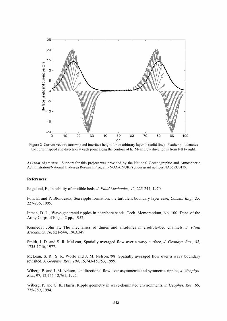
342

Figure 2 Current vectors (arrows) and interface height for an arbitrary layer, h (solid line). Feather plot denotesthe current speed and direction at each point along the contour of h. Mean flow direction is from left to right.

Acknowledgments: Support for this project was provided by the National Oceanographic and AtmosphericAdministration/National Undersea Research Program (NOAA/NURP) under grant number NA06RU0139.

References:

Engelund, F., Instability of erodible beds, J. Fluid Mechanics, 42, 225-244, 1970.

Foti, E. and P. Blondeaux, Sea ripple formation: the turbulent boundary layer case, Coastal Eng., 25,227-236, 1995.

Inman, D. L., Wave-generated ripples in nearshore sands, Tech. Memorandum, No. 100, Dept. of theArmy Corps of Eng., 42 pp., 1957.

Kennedy, John F., The mechanics of dunes and antidunes in erodible-bed channels, J. FluidMechanics, 16, 521-544, 1963.349

Smith, J. D. and S. R. McLean, Spatially averaged flow over a wavy surface, J. Geophys. Res., 82,1735-1746, 1977.

McLean, S. R., S. R. Wolfe and J. M. Nelson,798 Spatially averaged flow over a wavy boundaryrevisited, J. Geophys. Res., 104, 15,743-15,753, 1999.

Wiberg, P. and J. M. Nelson, Unidirectional flow over asymmetric and symmetric ripples, J. Geophys.Res., 97, 12,745-12,761, 1992.

Wiberg, P. and C. K. Harris, Ripple geometry in wave-dominated environments, J. Geophys. Res., 99,775-789, 1994.

343

Spatial variation of diurnal tidal asymmetry around aprotruding delta frontBAS VAN MAREN

(Institute for Marine and Atmospheric Research Utrecht / IMAU, Utrecht University,Heidelberglaan 2, 3508 TC Utrecht, The Netherlands, [email protected])

PIET HOEKSTRA

(Institute for Marine and Atmospheric Research Utrecht / IMAU, Utrecht University,Heidelberglaan 2, 3508 TC Utrecht, The Netherlands, [email protected])

1. IntroductionThe Red River delta is the largest delta system in north Vietnam, and debouches in the Gulf of Tonkinby a number of distributaries of which the Ba Lat river mouth is the largest (Fig. 1). Themorphological evolution of the Ba Lat delta is characterised by periods of coastal accretion,alternating with periods of coastal erosion and a redistribution of sediment due to reworking by wavesand currents. Van Maren and Hoekstra (2003) presented a conceptual model that explains this patternwith the internal dynamics of the system, rather than by periodically varying boundary conditions suchas river discharge or wave power. This concept is presently being implemented and tested in anumerical model that is able to simulate the morphological developments of the subaquous delta inresponse to waves, currents and river discharge. Together with field data, this model is applied to testhypothesis about the morphologic evolution of the delta.

At present, the southern part of the delta front is rapidly accreting, while the northern part is eroding(Van Maren and Hoekstra, 2003). The reasons for this southward growth were observed to be asouthward sediment transport driven by tidal asymmetry, and southward advection of the turbid riverplume. In this paper we focus on the potential role of alongshore tidal currents for redistribution ofdelta front sediments by means of a numerical tidal model.

Figure 1 Distributaries of the Red River delta

2. Field methods and observationsCurrent velocities were measured in front of the river mouth during three 25-hour stations; one at neaptide and two during spring tide conditions. Water level variations were measured in the river mouth,

344

and supplemented with sparse available data from literature. The dominant tidal constituents in theGulf of Tonkin are O1, K1, and M2 (Fang et al., 1999) with amplitudes of about 50, 50, and 15 cm,respectively near the Red River Delta. The co-tidal lines of O1 and K1 in these regions of the Gulf ofTonkin are widely spaced due to resonance of the diurnal constituents (Fang et al., 1999). Thereforethe phase differences between the northern and southern part of the Red River Delta are only small forthe diurnal constituents, and the corresponding tidal wave celerity equals a value of approximately 30m/s. The M2 co-tidal lines are less widely spaced near the Red River delta, and related to a tidal wavepropagating with a speed of about 10 m/s.

The measured velocities in front of the river mouth were asymmetrical and diurnal during spring tides,with a short period of strong southward flow and a longer period of weak northward flow (see Fig. 2aand 2c). Nearly symmetrical semi-diurnal currents characterize the flow pattern during neap tide. Thisdifference in flow conditions is attributed to interaction of the O1, K1 and M2 tidal constituents, whichare able to induce a tidal asymmetry with a distinct periodicity (e.g. Hoitink et al., 2003). As thesediment transport capacity of the tidal currents is commonly proportional to the third power of flowvelocity, this asymmetry favours southward sediment transport. The tidal asymmetry is an importantmechanism that has to be reproduced correctly by the numerical model.

−50

0

50

(a)

v [cm/s]

H [cm]

−100

0

100

−50

0

50

(b) −100

0

100

0 6 12 18 24

−50

0

50

(c)

0 6 12 18 24

−100

0

100

Figure 2. Three 24-hour measurements of water level (right y-axis, in cm) and near-bottom current velocity (lefty-axis, cm/s, flood current positive) in front of the river mouth (for location; see panel (a) of Fig. 4). Panel (a)and (c) show spring tide measurements while neap tide measurements are given in (b). The flood current isdirected towards the south.

3. Modelling: setup and preliminary resultsThe current field is computed with the flow module of the Delft3D software package formorphodynamic modelling. The flow module, run in 2DH mode, is solving the non-linear shallowwater equations. The computational grid is curvilinear with 300*150 grid points, covering an area of30 km cross-shore by 70 km alongshore. Water level variations are prescribed on the northern openboundary and the southern open boundary as progressive tidal waves; the shore-parallel sea boundaryis closed. The ‘free’ parameters are the phase lag of the M2 constituent on the diurnal constituents, andthe propagation velocity of the semi-diurnal tidal wave and diurnal tidal wave. These three parameterscan be estimated and fine-tuned to reproduce the flow pattern in front of the river mouth. Using the

345

propagation velocities of 30 m/s for the diurnal components and 10 m/s for the semi-diurnalcomponent, only the phase lag of the semi-diurnal component relative to the diurnal component has tobe iterated until the flow patterns of Fig. 2 are reproduced. The resulting water level variation andcurrent velocities over two tidal cycles (spring tide and neap tide), at the same location were themeasurements took place, are shown in Fig. 3.

−1

0

1

a

−0.5

0

0.5

0 5 10 15 20 25

−1

0

1

b

−0.5

0

0.5

Figure 3. Model results in front of river mouth showing water level (thick line, left y-axis, in m.) and depth-averaged current velocity (right y-axis, m/s, flood current positive) in front of the river mouth (for location; seepanel (a) of Fig. 4). Panel (a) shows a spring tide simulation, and panel (b) a neap tide simulation.

6.4 6.6 6.8 7

x 105

2.21

2.22

2.23

2.24

2.25

2.26

2.27

2.28

x 106 a

−25−1

5−5

0

0.1

0.2

0.3

0.4

0.5

0.6

6.4 6.6 6.8 7

x 105

2.21

2.22

2.23

2.24

2.25

2.26

2.27

2.28

x 106 b

0

0.1

0.2

0.3

0.4

0.5

0.6

6.4 6.6 6.8 7

x 105

2.21

2.22

2.23

2.24

2.25

2.26

2.27

2.28

x 106 c

−0.01

−0.005

0

0.005

0.01

6.4 6.6 6.8 7

x 105

2.21

2.22

2.23

2.24

2.25

2.26

2.27

2.28

x 106 d

Figure 4. Model results for an M2 tidal wave travelling at a speed of 10 m/s and O1 and K1 tidal waves travellingat a speed of 30 m/s. The bathymetry is shown in panel (a), while maximum ebb (northward) and flood

(southward) velocities are given in (b) and (c) respectively (m/s). The transport capacity, defined as >< 3u , isgiven in panel (d); positive values are directed towards the south.

346

The southward current (positive) is stronger than the northward current, and the period of southwardflow is shorter, both agreeing with the results shown in Fig. 2. However, the propagation of a diurnaltidal wave and a semi-diurnal tidal wave is different due to e.g. bathymetric and frictional effects.Therefore the phase lags of the M2 currents on the O1 and K1 currents will spatially vary. The result isa spatially varying asymmetry, which is depicted in fig. 4b and 4c: areas with higher flood velocitiesalternate in an alongshore direction with areas were ebb velocities are higher. This spatially varyingdominance of ebb- and flood currents has implications for the sediment transport capacity of the tidalcurrents.

Erosion and deposition result from gradients in sediment transport. Flow contraction over the deltafront (see Fig. 4b and 4c) results in deceleration of the flow velocity, and therefore sediment transportcapacity, downstream of the deltafront. Therefore the southward tidal asymmetry on the delta front(Fig. 2 and 3) promotes deposition in the southern part of the subaqeous delta. The spatially varying

tidal asymmetry complicates this pattern. The transport capacity is parameterised by averaging 3u (thesouthward flood current as positive) over two tidal cycles (Fig. 4d). The strong spatial variation in thistransport capacity is indicative of sediment transport divergences and convergences, and therefore, ofspatial alternations of erosion and deposition. Southwest of the measurement location, where strongsouth-westward currents where measured, the model predicts stronger north-eastward currents. Thisimplies that sediment transport paths converge on the southern part of the delta front. North of thispoint ebb-currents dominate as well, producing a divergence of the sediment transport capacity.Therefore, the spatial variability of O1-K1-M2 tidal asymmetry may be another mechanism thatcontributes to the southward growth of the Ba Lat delta, in addition to the southward advection ofsuspended river plume sediments as described by Van Maren and Hoekstra (2003).

4. Discussion and conclusionsAs a first order estimate, boundary conditions are prescribed by progressive tidal waves. Although theasymmetry of the current pattern is reasonably reproduced, the phase lag of water levels on thecurrents is not correct. While the currents lead the water levels according to the numerical model (dueto frictional effects on the enforced progressive wave), the opposite was observed. The currents lag thewater levels in Fig. 2, which is caused by resonance of the diurnal components in the northern parts ofthe Gulf of Tonkin. This will affect river outflow patterns, residual transports by the Stokes drift, andthe spatial distribution of the flow asymmetry. Implementation of standing waves is part of futureresearch.

Tidal asymmetry and flow contraction on the delta front favour a southward growth of the delta front.In addition, spatially varying tidal asymmetry results in alongshore alternations of sediment transportcapacity divergence and convergence, which might result in erosion and deposition patterns. Althoughthe spatially varying asymmetry of the tidal currents is highly sensitive to the imposed phase lags inthe boundary conditions, a spatial varying pattern does arise for every calculated scenario. The resultis that a large disturbance, in this case a delta front, can affect the O1, K1 and M2 constituents in such away that the resulting asymmetry further promotes or counteracts the growth of the disturbance.

References

Fang, G., Kwok, Y. K., Yu, K., and Zhu, Y. (1999), Numerical simulation of principal tidal constituents in theSouth China Sea, Gulf of Tonkin and Gulf of Thailand. Continental Shelf Research, 19(7), pp. 845-869.

Hoitink, A. J. F., Hoekstra, P., and Van Maren, D. S. (2003), Flow asymmetry associated with astronomicaltides: implications for the residual transport of sediment. Journal of Geophysical Research C: Oceans, SubmittedVan Maren, D. S. and Hoekstra, P. (2003), A model for cyclic delta growth; the Ba Lat delta, Vietnam. Journalof Asian Earth Sciences, submitted.

347

Hydrodynamics across a channel-shoal slope in the ebbtidal delta of Texel, the Netherlands.SANDRA VERMEER

(Utrecht University, P.O. BOX 80.115, 3508 TC Utrecht, the Netherlands,[email protected])

AART KROON

(Utrecht University, P.O. BOX 80.115, 3508 TC Utrecht, the Netherlands,[email protected])

1. IntroductionEbb tidal deltas are highly dynamic morphological features on the seaward side of tidal basins. Theyplay an important role in the exchange of water and sediment between the tidal basin and the coastalzone. The interaction between the hydrodyamic conditions in and outside the inlet (waves, tides,winddriven currents, etc.) and the morphology of the ebb tidal delta provide for the sedimentbypassing over the outer delta and thereby affect the stability of the adjacent barrier islands.

Sediment by-passing in ebb tidal delta systems is a well studied phenomenon (e.g. Bruun andGerritsen, 1959; Bruun, 1966; Oertel, 1972; Nummedal and Penland, 1981; Hanisch, 1981;FitzGerald, 1982, 1988). However, these studies focus on the large scale behaviour of sediment pathsbut neglect the detailed sediment movement processes.

The aim of this research is to increase our knowledge of small scale hydrodynamics and sedimenttransport processes in a channel-shoal transition area on an ebb tidal delta. The hydrodynamicconditions are studied on a monthly time scale, twice a year in 2001 and 2002. The morphologicalchanges are investigated over a period of 10 years, showing the morphological development of thechannel-shoal transition area at the southern part of the Noorderhaaks shoal.

Figure 1: Left panel: Location of the ebb tidal delta of Texel, Right panel: Depth contours of the ebb tidal deltaof Texel with the location of the channel-shoal area (box) and cross-channel transect (line).

2. SettingThe study area is situated on the ebb tidal delta of Texel, the Netherlands (Figure 1, left panel). Thelocation of the experiments is south of the shoal Noorderhaaks and on the upper slope of the channelSchulpengat (Figure 1, right panel). This area is indicated as the channel-shoal transition area, from

348

–10 m to –2.5 m depth, where tidal and wave processes act upon and interact. The local morphology isseparated in two zones: an upper slope and a lower slope area. The upper slope of the transition area,which is the deeper part of the shoal Noorderhaaks, inclines mildly around 1-2%. Mega ripples are themain bottom structures (height about 40-60 cm and length over 100 m, from local observations). Thelower slope is steeper (up to 7%) and coincides with the upper slope of the channel Schulpengat. Thispart is situated in the outer channel bend. Bed forms mainly consist of oblique sand waves.

3. Morphological development 1986-1997Figure 2 (left panel) shows the accretion and erosion patterns on the ebb tidal delta of Texel during theperiod 1986-1997. The black to gray colours indicate erosion and the gray to white accretion.

The middle supratidal part of the Noorderhaaks moved southward and expanded to the north and southat the western end. The situation is more complicated on the eastern side. The northern part of thechannel Molengat migrated towards the east, thereby eroding the beach of Texel, while the southernpart of the channel branched off to a northwestern direction. The southern part of the Noorderhaaksshows alternating stripes of erosion and accretion. For instance, the northern fringe of the Schulpengatchannel eroded, while the Westgat was filled with sediment.

Figure 2 (right panel) shows two transects south of the Noorderhaaks in detail. The dynamic area isindicated by the box. The lower slope of the shoal Noorderhaaks, at a depth of about –3 to –5 m belowmean sea level, increases in height by 0-0.5 m/yr, while the upper channel slope at a level of –10 merodes at a rate of 12-13m/yr. This implies an overall increase of the channel slope. The fieldexperiments are executed in this area.

Figure 2: Left panel: Accretion – erosion patterns (in meters) in the ebb tidal delta of Texel, 1986-1997; Rightpanels: Transects from Noorderhaaks and the channel Schulpengat, orientated northwest-southeast. Top panel isthe eastern transect, the lower panel the western transect, tripod transect (see Figure 1) is situated in between.

4. Hydrodynamics

Currents

The tidal wave on the North Sea travels from south to north along the Dutch coast and propagate intothe tidal inlet from southwest. The tidal current ellipses in the study area have a bidirectional characterwith a northeast – southwest direction.

0 500 1000 1500 2000 2500 3000-4000

-3500

-3000

-2500

-2000

-1500

-1000

-500

0

dept

h (c

m)

19861997

0 500 1000 1500 2000 2500 3000 3500-3500

-3000

-2500

-2000

-1500

-1000

-500

0

distance (m)

349

The hourly averaged mean currents as observed at –10 m depth (Figure 3, left panels; for location seeFigure 1) show a barchan shaped cloud of dots. Each dot represents averaged velocity measurementswhich were sampled each hour with a frequency of 2 Hz over 34 minutes. The shape indicates adownslope directed (secondary) current, which can be associated with the secondary downslopedirected current in the outer bend of a river channel (personal communication Van Aken, 2002; VanRijn, 1994).

Figure 3: Left panel: mean current during June 2001 and October 2001 at –2.5 m (left panel) and –10 m depth(right panel). The x-axis represents the longshore direction, the y-axis the cross shore direction, Right panel:tidally averaged mean current (25 hours), conditions indicated in Figure 4; Depths: –10 m (D), -7.5 m (C), -4.5m (B) and –2.5 m (A).

The tidally averaged mean current (25 hour resultant vectors) over the cross-shore profile show aspatial pattern (Figure 3, right panel) with an increase of the velocity direction towards the slope fromdeep water (tripod D at –10 m) towards the shore (tripod A at –2.5 m). However, the velocitydecreases from 0.24 m/s at deep water (tripod D) to 0.18 m/s at shallow water (tripod A). The netvelocity vectors point at an ebb dominance in the channel-shoal transition area. The difference indirection of the mean current between tripod A and D (see also Figure 3, left and middle panels) istheoretically due to the generation of vorticity by bottom friction and the Coriolis force (Van deMeene, 1994).

Figure 4: Upper left panel: significant wave height (A,C), lower left panel: wave direction (A,C) during June2001. The box indicates the conditions for Figure 3, right panel. Right panel: wave asymmetry at –7.5 m (C) and–2.5 m (A) depth.

Waves

Figure 4 (upper en lower left panels) shows the wave conditions during June 2001. In this period ofone month, higher wave energy conditions with local significant wave heights over 0.5 m alternate

350

with lower wave energy periods. The dominant wave direction during this month is south-southwest.This direction often differs from the wind direction. This is caused by refraction and the shelteringeffect of the Noorderhaaks in the North and West, the coast of North-Holland east of the tripods andthe location of the tidal inlet in the northeast.

The waves on the channel-shoal transition zone transform when they propagate from deep to shallowwater.

Firstly they refract on the depth contours and tidal currents and secondly they become asymmetrical.

The refraction of the waves is shown in Figure 4, lower left panel. The waves refract from a west-southwestern direction at a water depth of 7.5 m (tripod C) towards a southern direction at a waterdepth of – 2.5 m (tripod A). The asymmetry of the waves is expressed by the velocity ratio:

)UU(

UA

off,orbon,orb

on,orb

++++====

Where Uorb,on is the significant onshore component of the orbital velocity and Uorb,off is the significantoffshore component of the orbital velocity.

The asymmetry of all measured bursts is presented in Figure 4, right panel, where it is plotted againstthe local relative wave height, defined as the local wave height (H) divided by the local water depth(h). The waves near tripod C are almost symmetrical, whereas they become more asymmetric inshallow water dephts (tripod A). This asymmetry clearly increases with an increase of the localrelative wave height.

5. ConclusionsThe results from the hydrodynamic measurements and the erosion-accretion map indicate thatprocesses involved with curved flow in a channel bend, provide for the morphological development inthe lower part of the channel-shoal transition area.

In addition, the wave asymmetry, the dominant wave direction and the tide averaged currents indicateto provide for the observed accretion on the higher part of the channel-shoal transition area.

Further analysis of ADCP data, deployed in the channel-shoal transition area should give moreindications for the processes as described in this paper.

Acknowledgements: This research is part of the `Outer Delta Dynamics’-project, initiated by the NetherlandsCentre for Coastal Research (NCK) and financed by NWO/ALW (the Netherlands Organization for ScientificResearch). Shipping time was provided by the NIOZ (Netherlands Insitute for Sea Research) and also partner inthis project. The tripods were supplied by the Direction North Holland of the Ministry of Transport, Publicworks and Water management.

ReferencesBruun, P. (1966) Tidal inlets and littoral drift. Universiteitsforlaget, Trondheim, Norway.

Bruun, P. and Gerritsen (1959) By-passing of sand by natural action at coastal inlets and passes. Proc.ASCE, J. Waterways and harbour Div., Vol. 85, WW4.

FitzGerald, D. M. (1982) Sediment bypassing at mixed energy tidal inlets. Proceedings of theEighteenth Coastal Engineering Conference(November 1982), Cape Town, South Africa. ASCE, p1094-1118.

351

FitzGerald, D. M. (1988) Shoreline erosional-depositional processes associated with tidal inlets. Vol29, New York, Springer-Verlag. Lecture notes on Coastal and Estuarine studies, p 186-225.

Hanisch, J. (1981) Sand transport in the tidal inlet between Wangerooge and Spiekeroog (W.Germany). Special Publs.Int.Ass.Sediment 5, p 175-185.

Nummedal, D. and Penland, S. (1981) Sediment dispersal in Nordeneyer Seegat, WestGermany.Special Publs.Int.Ass.Sediment 5, Oxford, Blackwell Scientific Publications, p 187-210.

Oertel, G. F. (1972) Sediment transport of estuary entrance shoals and the formation of swashplatforms. Journal of Sedimentary Petrology 42 No. 2, p 857-863.

Van de Meene, (1994) The shoreface-connected ridges along the central Dutch coast. Thesis, KNAG /Netherlands Geographical Studies, 222 p.Van Rijn, L. C. (1994) Principles of fluid flow and surface waves in rivers, estuaries, seas and oceans.Aqua Publications, Oldemarkt, 335 p.

��

��

��

��

��

�� !"!�!��#�� !�� !�� !$!�!�!��#�� !�� !��

� ��

�� %�� &�� %�'�� (�� )� �� % �� *�� "�� %�� "�+��! ,�� "��+�� % �� -�� )��% �� ""�� -�� "�� .'��"�� "�+�� "�� "� � �� "�+�� %� �� %�� )��%! ��" � �� "�� "�� )� ��"�� %��+�� %�� "�� %�� ""�� /� �� 0�� "�� "�� %� � �� !

��

1�� "�� )��% �� '�� 23�� /��04 3�� 5 �� /�66604 7 /�66809! ��'�� )�� %'�� &�� )��%�� "�� "�� "�� "�+�� :�� ; �<��:� 2�� /�:��09 �� $�� "��%�� % ��% �� *��'��! �� "�� =�� %�� "�� )� � ��%��% �� !��!�!

>��?� /�6680 �� "�� %� �� "�� )�� )� *�� "��! �� )�� "��'�� ; ��

�� "�� <� ��+�� ; �

��

��

�; ��

�� <� ; �

��! >�� "�� %�� "��

�� *��! � �� %�� >�� /�6680 ��

�

��

��

��

��

��

ν��

��

�

��

��

��

��

�

��

@�%�� /�0 1�"��% "�� >�� /�6680 2��9 /�0 �� "�� %�� "�� ; /A0 �!��/Æ0 �!� �� /�0 �!� 2��9

"�� %�� @�%�� ! �� )�� "�� "�� "�� %�� "�� />�� 5 B�� 3��)� ��0!

� ��

�� "�� C� ��"�� % � �� /�6680! �� " �� )�� %�� "�� ! �� % " �� :��

�

�� ;� :��

� � �� :� �� ! >�� :� �� "�� )��%� �� ; �� "�� %��+�� %�� ; ��D! 7�� +�� ;��

�

��

� �! E� �� "�� ="�� !�!�:��

�� ; ��=" /��0 �� "�� %

%�� ! E� �� C� ��"�� - / �� 0 �� % ��"�� !�!�:� ; /<��

��:�0 A ��

� �� !

� ��

� �� % �� ""�� %�� 23�� /�6660� 3�� /��09

��

�:��

�

�:�

��

�:�

�; � A � � :� /�0

� �� *�� )�� % "�� ! �� /�0 �� "�� )��% ��&�� :��

�:��:�� &�� Æ�� :�� ! �� -�= �� %�� % �� +��

�

� � �� !��

ε��

�

��

��

��

��

�

��

� � �� !��

ε��

�

��

��

��

��

�

��

��

@�%�� /�0 � "�� &�� "�� &�� D�� "�� 4 /A0 �� )�� /Æ0�� )�� /�0 �� )� �� /�0 �� )� 2��9/�0 � "�� "�� &�� "�� F;��)� 4A �;�� Æ �;�� ;D�� ;�� ;�� ;�� 2��9

�� ; ��

��

��! E� �� !�!� ��:� ;

�! (��% � �� " :�� /:�0 �:��:� ; �� G<��

��D� ��

/�0 �� ""�� %�� *�� *�� "��

�� A

��

��

�

��

�

�

�� A

��

��

�

��A

��

�; � /�0

�� ; �� ; ��! �� .�� % ��=�� <�� - ! �� % �� "�� <��! �� "�� "��! >�� ; G�D�! �� /:�! :�! :��0 ;/<��! �! <��0 �� %��! E� �� %��+�� %�� ""�'"�� &�� Æ��! �� ="��'�� % ��%:�� ; "� /��#0

�

� ��! >�� "� ; �� !

� � ��

�� "�� "�"�� "�� "�� "�� %�� =�� "��!3�� "�� "�� ! �� "�� "��% ��=�� "�� 2 �� 9! E� �� "�� %�� %��+�� %�� "��!�� "�� "�� H,�(I�� "��!

E� � �) �� F;�� )� �� %%�� )� � ��%��+�� "�� "��% �� "�� $�� %�� J�� "��% �� ! E� � �� @�%�� /�0 �� %�� 8 � ��

D

�� %� � �� "�� "�� )� �� D�� "��

$�� /�J�0 ��

�� /�0 &� /��0 ��# �

� �!�K �!K K!� �!�� !�� !K� �!G �!8 �!�� !8�� !�� D!8 6!8 �!�D �!8K�� !�� !K ��!� �!�D �!8�� !�6 �!� ��!� �!�DG �!8�� !�� 6!� �D!� �!�KD �!�G

��%� � �� "�� D� �! �� D�L �� =�� "�� !�! �� @�%�� /�0 �� %�� "�� %�� "�� &�� "�� )�! @� �� "�� "�� "� �� %�� ! @� �� "�� % %�� "�� 8� � ��G�! @� ��"�� %�� G� � ��!

� ��

�� "�� ""�� +�� "�� &�� )��% �� '-�� "�� "��+� "��"�� "��%�� % ��%�� *��! �� % ��!

2�9 �� "�� %�� "��%�� "��%�� %��+�� Æ�� '��!2�9 �� "�� %�� )��%%��% �� "�� "�� "�� !2D9 @� ��"�� "� '/��0 �� )��% ��-�� % �� "�� "�� !8� �� ""�"��!2K9 �� %%�� )��% �� ""�� %��+�� "�+�� &�� %��% �� "� � ��%�'�� !�!� �� )� �� !

� � � � �

2�9 3�� >!� �� (��% �� '�� )��% �� *�� D�DD'D�K�

K

2�9 >�� (!H!1!>! 5 �� 3��)� M!1!� �� N�"�� "�� )� �� (�� N�� 6D��'6DDG

2D9 �� !�!� O�� 1!�!� �%�� P!N!� O�� I!1� C�� C!C!�I�� EEE� �!H!� > ��%� �!�!� 5 C��%��)�� (!�! � �668� �� )�� % ��"�� )��% �� 6�'G��

�

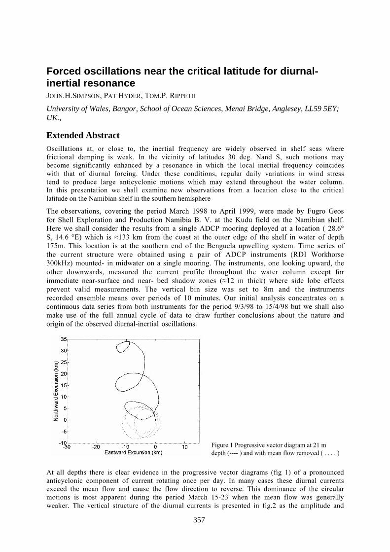
357

Forced oscillations near the critical latitude for diurnal-inertial resonanceJOHN.H.SIMPSON, PAT HYDER, TOM.P. RIPPETH

University of Wales, Bangor, School of Ocean Sciences, Menai Bridge, Anglesey, LL59 5EY;UK.,

Extended AbstractOscillations at, or close to, the inertial frequency are widely observed in shelf seas wherefrictional damping is weak. In the vicinity of latitudes 30 deg. Nand S, such motions maybecome significantly enhanced by a resonance in which the local inertial frequency coincideswith that of diurnal forcing. Under these conditions, regular daily variations in wind stresstend to produce large anticyclonic motions which may extend throughout the water column.In this presentation we shall examine new observations from a location close to the criticallatitude on the Namibian shelf in the southern hemisphere

The observations, covering the period March 1998 to April 1999, were made by Fugro Geosfor Shell Exploration and Production Namibia B. V. at the Kudu field on the Namibian shelf.Here we shall consider the results from a single ADCP mooring deployed at a location ( 28.6°S, 14.6 °E) which is ≈133 km from the coast at the outer edge of the shelf in water of depth175m. This location is at the southern end of the Benguela upwelling system. Time series ofthe current structure were obtained using a pair of ADCP instruments (RDI Workhorse300kHz) mounted- in midwater on a single mooring. The instruments, one looking upward, theother downwards, measured the current profile throughout the water column except forimmediate near-surface and near- bed shadow zones (≈12 m thick) where side lobe effectsprevent valid measurements. The vertical bin size was set to 8m and the instrumentsrecorded ensemble means over periods of 10 minutes. Our initial analysis concentrates on acontinuous data series from both instruments for the period 9/3/98 to 15/4/98 but we shall alsomake use of the full annual cycle of data to draw further conclusions about the nature andorigin of the observed diurnal-inertial oscillations.

Figure 1 Progressive vector diagram at 21 mdepth (---- ) and with mean flow removed ( . . . . )

At all depths there is clear evidence in the progressive vector diagrams (fig 1) of a pronouncedanticyclonic component of current rotating once per day. In many cases these diurnal currentsexceed the mean flow and cause the flow direction to reverse. This dominance of the circularmotions is most apparent during the period March 15-23 when the mean flow was generallyweaker. The vertical structure of the diurnal currents is presented in fig.2 as the amplitude and

358

phase of the anti-clockwise component which dominates over the almost negligible clockwiseflow. The oscillations have the greatest amplitude in the surface layer but energetic motions(speed > 0.2 m/s) occur in the bottom layer where the flow is ~180 degrees out of phase withthe upper layer. This phase change which occurred progressively between ~40 and ~ 110mdepth was a persistent feature of the flow and was associated with a minimum amplitude ataround 80m depth.

Figure 2.Vertical structure of (a) the amplitude of the anti-clockwise (*) and clockwise (+) diurnal currentcomponents and (b) the phase of the anticlockwise component

Unfortunately wind data were not recorded at the mooring location. The nearest source ofwind data is the airport at Oranjemund which is close to the Namibian coast but ~ 150 km fromthe current meter mooring. Time series from this source provide clear evidence of markeddiurnal variations in the windstress associated with the sea breeze regime which is a wellknown feature of this coast. The mean stress at oranjemund is mostly directed to NE withvalues up to 0.04 Pa but considerably stronger stresses are associated with the high frequencyvariations. Cross-shore and along shore components have maxima of comparable amplitude inmid-late afternoon (1500-1800) with peak stresses exceeding 0.1 Pa. and much weakeroffshore stresses at night. The cross-shore and along shore diurnal components of the windvector are almost in phase so the motion is approximately rectilinear at 45o to the coast, i.e.N-S, and consists of nearly equal clockwise and anticlockwise components.

The picture that emerges from the observations is of a current system in which strong diurnal-inertial oscillations are superimposed on a weaker mean flow to the north. The verticalstructure of the diurnal motions consists of two layers oscillating with comparable kineticenergy but ~ 180 degrees out of phase. This form of vertical structure and the intensity of thecurrent response may be understood in terms of a simple analytical model. . We considerflow in a shelf region bounded by a coastline extending in the y direction at x=O and with adepth profile H (x). The layers are assumed to be uniform but decoupled from each other by africtionless interface while the motion is forced by an oscillatory windstress (τ x , τ y) at thediurnal frequency ω. The momentum equations may be written for the upper and lower layersrespectively as:

(1)

(2)

359

where η is the surface elevation. Providing that the shelf width L is small in relation to the

barotropic wavelength 2 1 2π( )gH / /ω , we may employ the lowest order vertically-integratedsolution (Craig 1985) in order to determine the surface slope as:

(3)

Because of the no-normal-flow condition at the coast, the diurnal cross-slope stress τx inducesan opposing surface slope. Similarly the along-shore windstress τy drives a coast-parallel,depth uniform current V= i τy/(ωgH) which, in geostrophic balance, requires a surface slopecomponent of amplitude (f/ω) τy. Substituting equation (3) into (1) and (2) and defining thecomplex velocity w=u+iv = Weiiωt, we have the steady state solutions for anti-clockwisemotion as:

(4)

where γ =h2/h1 . Close to the resonant latitude in the southern hemisphere f/ω => -1 so that

(5)

This result indicates that the phase of the motion will differ by 180 degrees between the twolayers and that the ratio of the velocity amplitude in the two layers will be γ which is of order unity inthe present case so that upper and lower layer motions will be of comparablemagnitude. While the anticlockwise response will be enhanced at latitudes close to 30degrees South where f= -ω, the response to cyclonic forcing (ω = f) at the diurnal frequencyis considerably weaker by a factor of l (f+ω)/ (f-ω). This ratio has a value of ≈47 for latitude28.6 degrees south so that, for equal forcing, anti-clockwise motions should be minimal asobserved. The ratio of the depth mean current amplitudes in the upper and lower layers is ≈1.7 (figs 5 and 10) which is consistent with a value of y based on layer thicknesses h1 = 65mand h2 = 110m.

Because the wind data was not recorded locally, it is not possible to demonstrateunequivocally that these unusually large oscillations are due to local wind forcing alone. Aninteresting, alternative mechanism which might account for the enhancement of energy nearthe critical latitude is the turning of near inertial internal waves (Fu 1981). Such waves ofdiurnal frequency, having been generated by wind forcing in lower latitudes, propagatepolewards to be arrested at their "turning latitude" of30 degrees with a consequent peak inenergy in the diurnal band at this latitude. Three results from our analysis of the full dataseries of ~400 days are against such non-local generation:

i) The annual cycle of the diurnal windstress at the coast is reflected to a significant degree inthe current amplitude

360

ii) The phase of diurnal oscillations, determined daily, shows a considerable degree ofconsistency throughout the year but particularly during the summer period when diurnal windforcing is greatest.

iii) The consistent vertical structure over the annual cycle does not show indications of thephase and energy propagation commonly observed in deep-ocean observations of inertialmotions.

The near-resonant response observed in this case involves an efficient transfer of momentumand energy from the wind field to the current system with the diurnal motions dominating thekinetic energy spectrum. The anti-phase motions in top and bottom layers involve substantialvertical shears which will tend to promote dissipation and vertical mixing through the watercolumn. In shelf areas with significant diurnal winds and located close (±10o) to the criticallatitude, this energy source may be an important mechanism for inducing mixing betweenupper and lower layers. Where, as in the case considered here, tidal forcing is weak, motionsin the diurnal-inertial band may be the dominant mechanism for vertical exchange through astratified water column.

References

Craig P.D. (1989a) Constant eddy-viscosity models of vertical structure forced by periodic windsContinental shelf Research 9(4), 343-358.

Craig, P.D. (1989b) A model of diurnally forced vertical current structure near 30° latitude.Continental Shelf Research, 9 (11), 965-980.

Fu L.L. (1981) Observations and models of inertial waves in the deep ocean. Rev. Geophys. SpacePhys. 19, 141-170

361

First results of a study on the turbulent mixed layer in theBaltic SeaHANS ULRICH LASS

(Baltic Sea Research Institute Warnemünde, Seestr. 15, D-18119 Rostock, Germany, [email protected])

HARTMUT PRANDKE

(ISW Wassermesstechnik, Lenzer Straße 5, D-17213 Petersdorf, Germany, [email protected])

HANS BURCHARD

(Baltic Sea Research Institute Warnemünde, Seestr. 15, D-18119 Rostock, Germany,[email protected])

1. IntroductionAn understanding of turbulence is a key goal of the dynamics of the surface layer of the ocean sinceturbulent processes are crucial in controlling the exchange of momentum, dissolved and particularmatter between the atmosphere and the ocean. Until recently our knowledge of turbulence in thesurface mixed layer has been severely limited by the difficulties of making measurements of thefluctuating velocity components near the sea surface remote from a disturbing platform (ship) carryingthe necessary equipment.

Using free falling dissipation profiler the high wave number range of the turbulence was accessible.Oakey and Elliott (1982) could show that a constant fraction of the energy flux in the atmospheric

boundary layer, namely 3*8u , appears as dissipation in the mixed layer. Measurements below breaking

surface waves revealed a layer of enhanced dissipation where dissipation could not be scaled by thewall-layer scaling, Agrawal et al. (1992). Anis and Moum (1995) observed by means of a risingdissipation profiler vertical profiles of dissipation in the surface boundary layer. They observed adepth dependence of the dissipation close to exponential with a decay rate on the order of the inversewave number of the waves, suggesting wave-related turbulence in the upper part of the ocean surfaceboundary layer. Moreover, they suggest that high levels of turbulent kinetic energy are produced in athin surface layer with thickness of the order of the height of the breaking waves.

Shallow (50 m deep) banks in the central parts of the tide less Baltic Sea provide a suitable site forperforming reliable turbulence measurements with bottom mounted instrument carrier. This gives agood opportunity to study the surface mixed layer dynamics in relation to surface gravity waves in astratified water body remote from the shores.

2. Methods and dataMeasurements have been performed in the central Baltic Sea, from 30 August to 7 September 2001aiming at the estimation of the turbulent energy balance of the surface mixed layer. Time series ofprofiles of turbulent kinetic energy dissipation were measured by a rising dissipation profiler. Theprofiler was positioned with bottom mounted idler pulley outside the area where the ambientturbulence is disturbed by the anchored ship, see Figure 1 (for details, see Prandke et al., 2000). Thedissipation profiler started from a depth well below the seasonal thermocline and rose up to the seasurface. Six profiles were taken every hour in a burst mode. Complementary measurements comprisedtime series of hourly CTD profiles extending from the sea surface to close to the bottom, of hourlycurrent profiles measured with a bottom mounted ADCP, of hourly wave spectra measured with apressure recorder SBE 26 moored in about 5 m below the sea surface, of momentum and of buoyancy

362

fluxes through the sea surface calculated from continuous time series of the correspondingmeteorological parameters measured on board the research vessel.

Figure 1: Scheme of dissipation measurements with a rising dissipation profiler from the anchored R/VProf. A. Penck

3. Observational resultsThe wind forcing at the sea surface was characterised by a sequence of calm phases followed by windevents of moderate strength during the observations. The typical summer stratification of the BalticSea consisted of 17°C warm brackish surface water and 4°C cold intermediate winter water. Bothlayers were separated by a strong thermocline located at about 25 m depth. A special wind eventforced a group of inertial waves at 4 September 2001, while weak inertial oscillations where prevailingbefore this event.

Two physically different dissipation regimes could be observed, see Figure2. The first, the internaldissipation regime, was quite independent of the local wind speed. It featured a maximum located inthe seasonal thermocline and was most intense after the wind event that generated strong inertialwaves. The second, the surface dissipation regime, was closely correlated to the local wind speed. Ithad a maximum at the sea surface. An injection layer of turbulent energy was observed near the seasurface which was roughly one significant wave height thick. About one third of the total turbulentenergy flux through the sea surface was dissipated within the injection layer.

A transport layer of turbulence was observed below the injection layer. The dissipation rate ofturbulent energy decayed exponentially with depth within the transport layer. The decay rate dependson the local wind. The dissipation rate of the transport layer decreased to values of the internaldissipation regime at a depth zi=2U2/g, where U is the wind speed at 10 m above the sea surface and gis the gravity of the earth.

The vertical integrated dissipation rate of the surface dissipation regime is balanced by the flux ofturbulent kinetic energy through the sea surface (8u*

3 according to Oakey and Elliott, 1982). This fluxwas found to be not significantly different from the energy loss of surface waves by wave breakingaccording to Longuett-Higgins (1969).

The surface dissipation regime can be described by the relation kzoez εε =)( , where

sigo H

u

3

8 3*=ε and

k is the characteristic wave number of the wind waves 210U

gk = . Hsig is the significant wave height,

363

o

uρτ=2

* with the wind stress τ and the density of sea water oρ and the wind velocity at 10 m height

above the sea surface U10.

Figure 2. Isopleths of dissipation of turbulent kinetic energy (grey scale coded) and water temperature (contourlines) during the cruise. The gaps are due to technical problems with the stern anchor of the research vessel.

The normalised dissipation rate measured in the surface regime is shown in Figure 3.

Figure 3. Profiles of turbulent kinetic energy dissipation normalised with respect to depth and dissipation.

4. Numerical Modelling

In order to better interprete the observed dissipation rates, a simulation with a 1D water column modelwill be performed. Initial and surface boundary conditions will be taken from observations as well asthe vertical velocity which will be analysed from CDT-casts. The model includes a generic two-equation turbulence closure model recently suggested by Umlauf and Burchard (2002) which is able toresolve the transport layer and the underlying shear layer, but parameterises the injection layer whichis calculated by means of a surface roughness length depending on the wave height.

31.08.200 01.09.200 02.09.200 03.09.200 04.09.200 05.09.200 06.09.200 07.09.200

Epsilon [W/kg] (color) - Temperature [°C] (contour)

-30

-25

-20

-15

-10

-5

0

Dep

th [

m]

5E-010

1E-009

2E-009

5E-009

1E-008

2E-008

5E-008

1E-007

2E-007

5E-007

1E-006

2E-006

5E-006

1E-005

2E-005

5E-005

1E-004

REYNOLDS 08/2001

364

Acknowledgments: The authors are grateful to the captain, the officers and the crew of the researchvessel Prof. A. Penck who supported us during the field measurements. This work was supported bythe Federal Ministry of Research and Education of Germany under contract number 01LD0025.

References:

Agrawal, Y. C., E. A. Terray, M. A. Donelan, P. A. Hwang, A. J. Williams III, W. M. Drennan, K. K.Kahma, and S. A. Kitaigorodskii, Enhanced dissipation of kinetic energy beneth surface waves.Nature, 359, 219-220, 1992.

Anis, A. and J. N. Moum, Surface Wave – Turbulence Interactions: Scaling ε(z) near the sea surface.J. Phys. Oceanogr., 25, 2025 – 2045, 1995.

Longuett-Higgins, M. S., On wave breaking and the equilibrium spectrum of wind-generated waves.Proc. Roy. Soc. A., 310, 151-159, 1969.

Oakey, N. S. and J. A. Elliott, Dissipation within the surface mixed layer. J. Phys. Oceanogr., 12,171-185, 1982.

Prandke, H., K. Holtsch, and A. Stips, MITEC technology development: Themicrostructure/turbulence measuring system MSS. Tech. Rep. EUR 19733 EN, EuropeanCommission, 2000.

Umlauf, L., and H. Burchard, A generic length-scale equation for geophysical turbulence models, J.Phys. Oceanogr, 2002, submitted.

��

��

��

�� !�

��

�� !��"�� #�� $�� %��#�� !� �� $�� &�� '� �()�*+�� *)�,� �� -� �((�.�� ()�(�,� �� /��0� �� ! �� #��%�� 1�� $�� (��*+�� ,� �� 2�� ! �� 1 �� /34�,�� *++*��

$�� #��%��! � �� '� �� -� �� ! ��#��%! �� #�� $�� #�� ( � �+ � �� #��!�� !�� !�� 5 �� %��#�� %��#�� /34�,�� 1 �� 6� � �� 5 �� %�� 1� �� 1 �� %�� #�� $�� 5'-/ �� /34�,�� $�� 7�� !�� %�� !�� %�� $�� 8�� %��#�� 2�%�� #��

�� ! �� ! %� �7�� %!�2�� #�� %�� 8�� %��

� ��

5 �� 1� �� -4�,3,�� 9�!�� 3�� #�� / �� 9�!�� *++*%�� 5 �� %��#�� &�� #�� %�� !�� $�� ! �� ! �� %�� %� �� #��#� �� 6� � *�� 4� �� ! �%�� %��#�� $�� #�� #��

$� ��!�� #�� 8�� 7�� /34�,�� $�� &�� #�� #��#� �� #�� :� �� ! �� %� ��! �� 7�� '�� ! �� 9�!�� *++*�� #�� %�� *�� %�2 �� 8��

$�� 7�� %�� &�� *� � *) 4�%�� 6� .�� $�� !��#�� &�� %�� %�� 6� � .�� $�� #�� #�� 6� �� .%;� �� 8�� Æ�� 8�� %�� $�� %�� ! �� $�� %�� 7�� !�� %� �%#��! �� &�� $�� 7�� %�� #�� %��#�� .�' �� 7�� ! ��#��

��

$�� %�� #�� 8�� #� �� #�� ! �� #�� *��#� �� &�� .� ��

$� ��#� �� ! �� .�' �� #�� ;* 2� �� "�� ;* � �� #�� *� �� 7�� .� � ��8��#� �� #�� )� ��

��

�� <�� <�� =�� <�� *++*� /�� #�� 7�� /34�,�� <� �� 3��

9�!�� /�<�� <�� <�,�� /�� 3�� $�%�� 5�� $�� /�� >��5�� ?�� -4�,3,�� ; 5 �� !��!�� @ A�� '�� A�� 3�� A��

9�!�� /�<�� -�� A� �� B�� *++*� �� %�� %�! ��&�� C�� /34�,��%�� <� �� 3��

9�!�� /�<�� <�� <�,�� /�� 3�� *++*%� 5 �� ! �� #��%��! �� <� /�!�� 4��

�� 9�� D�� <�$�6�� 3��2�� #� ��%��! �� B��!�� 3�� 9�� *E� *��.;*��E�

6� �� @ $�� /34�,�� *� � *) 4�%��

6� �� *@ $�� &�� -� �� .+ 5� �� 1�@ �%��#�� #�� #��

6� �� .@ /34�,�� 4�%�� *� � *)� �A�� !��#�� &�� @ �%��#�� &�� $�� 8�� Æ��@ &��

370

Basin-scale interaction between tides and bathymetry in ashelf sea: morphodynamics of Taylor's problemJOHAN VAN DER MOLEN

(Institute for Marine and Atmospheric Research Utrecht (IMAU), Utrecht University,Princetonplein 5, 3584 CC Utrecht, The Netherlands, [email protected])

TACO MULDER

(same address, [email protected])

JEROEN GERRITS


HUIB DE SWART


1. IntroductionNumerical simulations of sand transport in the southern bight of the North Sea have indicated that afeedback mechanism exists between the tidal hydrodynamics and the basin-scale bathymetry (Van derMolen & De Swart, 2001). This feedback mechanism results in a co-evolving bathymetry andassociated tidal system on a time scale of thousands to tens of thousands of years. Results arepresented of a numerical study of the behaviour of this system. In particular, the question is addressedwhether this feedback process leads to morphodynamic equilibria equivalent to those that have beenfound for tidal basins of a size of tens of kilometers.

Equilibria between hydrodynamics and sea-bed topography, characterised by vanishing averagedivergence in the displacement of sediment, have been demonstrated to exist in tidal basins (e.g.,Schuttelaars & De Swart, 2000). Such equilibria arise from positive feedback between water motionand bottom topography during the initial stage of development, followed by a stabilising mechanismduring the final stage. If morphodynamic equilibria exist for tidal basins, it is worthwhile toinvestigate the possible existence of equilibria for larger basins like tidal shelf seas. Indeed, numericalmodel results of sand transport for the southern bight of the North Sea show overall smaller tide-averaged sand transports for the actual large-scale bathymetry when compared with results of a modelrun where all bathymetrical features within the southern bight were removed by assuming a flatbottom at average depth. This result indicates that the present southern bight may be in an intermediatestage of development towards a large-scale morphodynamic equilibrium. Geological observationsseem to support this presumption, they indicate large-scale marine erosion and deposition of 5 to 20 mfollowing the large-scale flooding of the North Sea as a result of the last deglaciation. These bottomchanges will have interacted with the hydrodynamics, because they are of the same order of magnitudeas the present-day mean water depth (~25 m).

The present study was carried out by using fully non-linear numerical models of the tidalhydrodynamics applied to an idealised basin with a geometry that represents the main dimensions ofthe southern bight of the North Sea. Local sand-transport formulations were used to compute theredistribution of sediment. Two morphodynamical models were applied: the existing Delft-3D-Mormodel of Delft Hydraulics (Wang et al., 1995), and a newly developed morphodynamical model(UMORPH) that uses the HAMSOM ocean circulation model (Backhaus, 1985) to calculate thehydrodynamics.

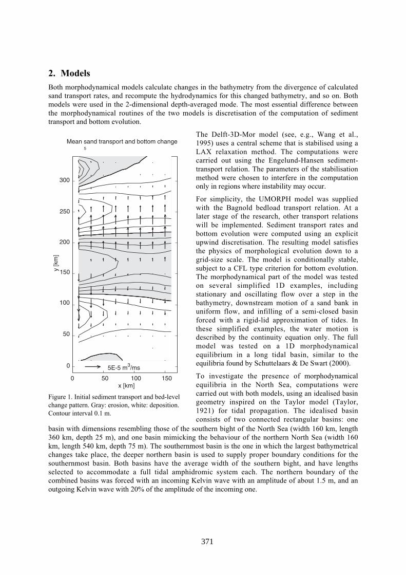
371

2. ModelsBoth morphodynamical models calculate changes in the bathymetry from the divergence of calculatedsand transport rates, and recompute the hydrodynamics for this changed bathymetry, and so on. Bothmodels were used in the 2-dimensional depth-averaged mode. The most essential difference betweenthe morphodynamical routines of the two models is discretisation of the computation of sedimenttransport and bottom evolution.

Figure 1. Initial sediment transport and bed-levelchange pattern. Gray: erosion, white: deposition.Contour interval 0.1 m.

The Delft-3D-Mor model (see, e.g., Wang et al.,1995) uses a central scheme that is stabilised using aLAX relaxation method. The computations werecarried out using the Engelund-Hansen sediment-transport relation. The parameters of the stabilisationmethod were chosen to interfere in the computationonly in regions where instability may occur.

For simplicity, the UMORPH model was suppliedwith the Bagnold bedload transport relation. At alater stage of the research, other transport relationswill be implemented. Sediment transport rates andbottom evolution were computed using an explicitupwind discretisation. The resulting model satisfiesthe physics of morphological evolution down to agrid-size scale. The model is conditionally stable,subject to a CFL type criterion for bottom evolution.The morphodynamical part of the model was testedon several simplified 1D examples, includingstationary and oscillating flow over a step in thebathymetry, downstream motion of a sand bank inuniform flow, and infilling of a semi-closed basinforced with a rigid-lid approximation of tides. Inthese simplified examples, the water motion isdescribed by the continuity equation only. The fullmodel was tested on a 1D morphodynamicalequilibrium in a long tidal basin, similar to theequilibria found by Schuttelaars & De Swart (2000).

To investigate the presence of morphodynamicalequilibria in the North Sea, computations werecarried out with both models, using an idealised basingeometry inspired on the Taylor model (Taylor,1921) for tidal propagation. The idealised basinconsists of two connected rectangular basins: one

basin with dimensions resembling those of the southern bight of the North Sea (width 160 km, length360 km, depth 25 m), and one basin mimicking the behaviour of the northern North Sea (width 160km, length 540 km, depth 75 m). The southernmost basin is the one in which the largest bathymetricalchanges take place, the deeper northern basin is used to supply proper boundary conditions for thesouthernmost basin. Both basins have the average width of the southern bight, and have lengthsselected to accommodate a full tidal amphidromic system each. The northern boundary of thecombined basins was forced with an incoming Kelvin wave with an amplitude of about 1.5 m, and anoutgoing Kelvin wave with 20% of the amplitude of the incoming one.

372

3. ResultsThe initial pattern ofsediment transport andbottom change for a flatbottom in the southernmostbasin is shown in Figure 1for the Delft-3D-Mormodel. Results of a similarmodel run with theUMORPH model arecomparable, except forlocal details. The large-scale pattern is similar tothat found with a numericalmodel of the North Sea(Van der Molen & DeSwart, 2001), and shows asediment-erosion zone withtransport to depositionareas in the north andsouth. The bottom-changepattern is periodic in thenorth-south direction, andfeatures exponential decay in the east-west direction towards a line east of the center of the basin. Thispattern resembles that of a stationary Kelvin wave, where the wave patterns along the eastern andwestern boundaries are approximately in phase in a spatial sense but have different amplitudes. Figure2 shows the bathymetry resulting from a 7200 year run of the Delft-3D-Mor model. The chosenstability coefficients did not allow longer simulations. The results show that the bottom wave patternhas grown substantially, while the general shape has remained more or less the same. The changes inbottom geometry cause an increase in the mean bottom friction which results in a shift of theamphidromic system towards the east. The amphidromic system is also shifted slightly to the north,which may result from a change in resonance characteristics of the basin caused by the depth changes.The current amplitudes are closely related to the changing bottom geometry and have decreased in theerosion area and increased in the deposition areas.

In Figure 3, results of the UMORPH model are shown after 320,000 years. The time spans of the twomodels cannot be compared directly because a total-load formulation was used in the Delft-3D-Mormodel, whereas a bedload formulation was used in the UMORPH model, resulting in a faster rate ofevolution for the Delft-3D-Mor model. The large-scale evolution of the UMORPH model is similar tothat of the Delft-3D-Mor model: erosion in the center and deposition in the north and south. Atapproximately the stage where the Delft-3D-Mor simulation was discontinued, linear bars are formed(not shown) that connect to evolve into the large-scale ridges shown in Figure 3 in the western part ofthe basin. At this stage of the model evolution, the ridges are near dynamic equilibrium with the watermotion: their shape has become more or less constant, although they do show some migration. In theeastern part of the basin, a complex pattern of banks evolves. Meanwhile, the larger scale basinevolution is continuing. Analysis of the water motion showed that flow velocities have a maximumover the ridges in the west, with major axes of the current ellipses oriented across the ridges and alongthe troughs between the ridges. Clockwise residual circulation cells exist around the ridges. Theamphidromic systems of the principle tide M2 and the overtide M4 are affected by the basin evolution,in particular those of the currents, that clearly reflect the sand-bank pattern. Net sediment transportsare largest at the crests of the banks, and show circulation of sediment around the banks, as well as nettransport across the crests that results in the migration.

Figure 2. Sea-bed topography after 7200 years in the southern basin, Delft-3D-Mor model.

373

More results of the UMORPH model will be presented at the conference, such as simulations withdifferent initial bottom topographies and computations with modified sediment-transport formulations.

4. ConclusionsThe following results were obtained:

• The initial bottom features which form in a shelf-sea basin with a geometry similar to thatused by Taylor (1921) and with a flat bottom have the characteristics of stationary Kelvinwaves.

• These large-scale features have the tendency to grow.

• At an early stage in the morphodynamic development of the model basin, local bedformsdevelop. These bedforms most likely represent conditions that are closer to local equilibriumthan a nearly flat basin floor, and (quite suddenly) evolve into larger-scale features as timeprogresses, while the total system continues to evolve. It is expected that this step like processwill repeat itself until full equilibrium is obtained.

Acknowledgments: The authors would like toexpress their gratitude to Prof. dr. JanBackhaus for making the HAMSOM modelavailable. WL | Delft Hydraulics is thanked forpermission to use the Delft-3D model. Theresearch was funded by the NetherlandsGeosciences Foundation (GOA) with financialaid of the Organization for Scientific Research(NWO) (NWO-grant 811.33.005).

References:

Backhaus, J.O., 1985. A three-dimensionalmodel for the simulation of shelf seadynamics. Deutsche HydrographischeZeitschrift 38, 165-187.

Schuttelaars, H.M., de Swart, H.E., 2000.Multiple morphodynamic equilibria intidal embayments. Journal of GeophysicalResearch 105 C10, 24105-24118.

Taylor, G.I., 1921. Tidal oscillations ingulfs and rectangular basins. Proceedingsof the London Mathematical Society 20,148-181.

Van der Molen, J., de Swart, H.E., 2001. Holocene tidal conditions and tide-induced sand transport inthe southern North Sea. Journal of Geophysical Research 106 C5, 9339-9362.

Wang, Z.B., Louters, T., de Vriend, H., 1995. Morphodynamic modelling for a tidal inlet in theWadden Sea. Marine Geology 126, 289-300.

Figure 3. Sea-bed topography in southern basin of theUMORPH model after 320,000 years. Depths in m.

374

Modelling the influence of artificial degassing on thestratification and the safety of Lake NyosMARTIN SCHMID, ANDREAS LORKE AND ALFRED WÜEST

(EAWAG, Seestrasse 79, CH-6047 Kastanienbaum, Switzerland, [email protected])

1. IntroductionLake Nyos is one of several crater lakes in the north-western part of Cameroon (Kling, 1988). Thelake has an infamous reputation since August 1986, when it released a large cloud of carbon dioxide(CO2), which flowed down the neighbouring valleys and asphyxiated 1700 people (Kling et al., 1987).With the exception of a similar gas burst of smaller scale at nearby Lake Monoun (Sigurdsson et al.,1987), this volcanological hazard had not been previously known. The disaster was followed by anintense scientific discussion about the origin of the gas burst. Two main hypotheses were set up(Sigvaldason, 1989). Following the limnic eruption hypothesis, high CO2 concentrations had slowlybuilt up in the lake column, and a large part of the CO2 was released after a trigger mechanism led tolocal oversaturation. The volcanic eruption hypothesis, on the other hand, ascribed the gas burst to asudden injection of CO2 from beneath the lake. The slow recharge of CO2 to the bottom water of thelake after the eruption (Kusakabe et al., 2000; Evans et al., 1994; Nojiri et al., 1993) strongly supportsthe limnic eruption hypothesis. Our work therefore is based on this hypothesis. Nevertheless it shouldbe kept in mind that sudden volcanic activity leading to similar disasters cannot be excluded in thisregion.

Since the renewal of high CO2 concentrations in the lake column could lead to a new disaster withindecades, a plan was set up to degas the lake. In January 2001, after several experimental tests inpreceding years, a first polyethylene pipe was installed in Lake Nyos. Water is taken in at a depth of203 m and released as a fountain on the lake surface. Due to the high CO2 pressure in the bottomwater, the water flow through the tube is self-sustaining, driven by the expansion of gas bubbles. Adetailed description of the degassing procedure can be found on the Lake Nyos degassing homepage(Halbwachs, 2002). However, there is concern that the degassing procedure, by lifting heavy bottomwater to the surface, could lower the stability of the lake column and impose the risk of a new eruptionduring the degassing process (Pickrell, 2001). Previous simulation results have suggested that thewater column below the epilimnion should remain stable during the degassing process (McCord andSchladow, 1998). However, this model did not include the effect of the geochemical cycling on waterdensity with the exception of CO2. The bottom water of Lake Nyos contains also large amounts ofdissolved reduced iron and other minerals. Transported to the surface, the iron will be oxidized andtransformed to amorphous iron hydroxide particles (Davison, 1993). The influence of the minerals andthe iron hydroxides on the density stratification is included in the model presented in this study.

2. Model DescriptionWe developed a one-dimensional model of Lake Nyos with a vertical resolution of 1m. The model isimplemented within the lake module of the software AQUASIM 2.0 (Reichert, 1994; Reichert, 1998),which is designed to concurrently simulate physical and biogeochemical processes in natural andtechnical aquatic systems. The simulation is driven by weather data (irradiation, wind speed,temperature, water vapour pressure, and precipitation). Figure 1 gives an overview of the mainprocesses included in the model which are shortly described below.

375

H2O, CO2, Fe2+, MinH2O, CO2, Fe2+, Min

CO2, O2Wind

Turbulent mixing

HSHC HW HEHA

Preciptiation & Runoff

Hgeo

Fe2+ ? Fepart

vsed

Fepart ? Fe2+

H2CO ⌠ HCO3- ⌠ CO3

2-

TemperatureIrradiationVapour Pressure

Outflow

Figure 1: Overview of the processes included in the simulation of Lake Nyos.

Water balance

The water balance includes precipitation to the lake surface, runoff from the lake catchment, and anexchange with a warm subsurface reservoir with higher concentrations of CO2, Fe and minerals. Thisexchange is considered the source for the observed increase in mineral concentrations and heat(Kusakabe et al., 2000) in the bottom waters of Lake Nyos. Whereas in reality the lake surface dropsbelow the outflow level during the dry season, the lake surface is assumed to be constant in the modelby closing the water balance with the surface outflow. The water flow through the degassing pipe isparameterized depending on the intake depth zin and on the partial pressure of CO2 at zin. The currentlyinstalled pipe has an intake depth of 203 m, a diameter of 14.5 cm, and an average water flow of 65l/s. However, it is planned to install further pipes within the next years.

Heat balance

The heat exchange between the lake surface and the atmosphere includes short-wave irradiation (HS),infrared radiation from the sky (HA), infrared radiation from the water surface (HW), latent heat flux(HE), and convection (HC) (Goudsmit et al., 2002; Henderson-Sellers, 1986; Imboden and Wüest,1995). The observed increase in temperature in the bottom water is simulated with the hightemperature of the water reservoir that exchanges with the bottom water. The exsolution of the CO2 inthe pipe leads to a heat loss of c. 20 kJ/mol CO2.

Turbulent mixing

The physical mixing of the lake is simulated with a buoyancy-extended k-epsilon turbulence model(Goudsmit et al., 2002; Burchard and Petersen, 1999; Rodi, 1980). Turbulent mixing is driven by theenergy introduced into the system by surface shear stress from wind forcing, and by negativebuoyancy due to heat loss to the atmosphere, the heat input to the lake bottom, and the uplifting ofheavy bottom water to the lake surface with the degassing pipe. The model includes the energytransfer from internal seiches to turbulent kinetic energy in the bottom boundary layer, because thecontribution of this mixing on sloping boundaries to diapycnal transport has been shown to beimportant (Gloor et al., 2000). The water density is calculated depending on temperature and theconcentrations of carbon dioxide, minerals, and dissolved and particulate iron.

376

Geochemistry

The observed annual inflow of 100-200 Mmol CO2 to the bottom waters of Lake Nyos (Kusakabe etal., 2000) is the reason for the risk of a new eruption. The three species carbon dioxide, bicarbonateand carbonate are supposed to be in equilibrium. At the lake surface, the CO2 concentrationequilibrates with the atmosphere. The pH is assumed to be in equilibrium with the partial CO2 pressureand the alkalinity defined by the mineral concentration.

Dissolved iron (Fe(II)) is transported to the surface with the degassing pipe where it is oxidized andtransformed to particulate iron hydroxide. The particles sink down and are resuspended in the anoxiczone below the thermocline.

Minerals, simulated with one state variable for the sum of Mg, Ca, K, and Na, as well as temperature,are also introduced into the lake from the subsurface reservoir and transported to the surface with thepipe. Altogether the degassing reduces density at the bottom (gas, minerals) and increases density inthe surface water (minerals) and below the thermocline (resuspension of particulate iron). Oxygen isset to saturation at the lake surface and is used up in the sediment in proportion to the estimatedbiological primary production.

3. Simulations and safety assessmentSimulations are performed for several years before the degassing of the system. The results of thesesimulations are compared with observed CTD and CO2 profiles to check the applicability of themodel. A mooring was deployed in November 2001 in Lake Nyos with 11 thermistors and 4 sedimenttraps. The mooring will be retrieved after one year, and the results together with new CTD profileswill be used to check the consistency of the model during one year of lake degassing.

To assess the safety of the degassing of Lake Nyos, the energy is estimated, which is needed to movewater from anywhere below the thermocline to a level where it is supersaturated with CO2, which is anecessary but not sufficient requirement for a limnic eruption to occur. This energy depends on thevertical distance between a water parcel and its level of supersaturation, and on the difference betweenthe potential densities at these two levels. It can be compared to the energy contained in the internalwaves in the lake observed with the moored thermistors. These simulations and energy calculationswill allow to identify the safest of a variety of possible degassing scenarios.

Sensitivity analyses are conducted to check the sensitivity of the simulations to parameters that haveeither a large natural variability (e.g. precipitation) or are only imprecisely known for Lake Nyos (e.g.CO2 input rate at the lake bottom, biological productivity).

At the PECS conference, we present the modelstructure and the model validation with availabledata of temperature, CO2, mineral and ironconcentrations. Figure 2 shows a preliminaryresult of a first simulation run. The simulatedtotal CO2 concentrations after 10 months ofdegassing show a mixed epilimnion with a depthof slightly more than 50 m and a mixed bottomboundary layer (BBL). Both these features of thelake column could be observed in the CTD datameasured in November 2001, even though theepilimnion was slightly less deep, and the BBLwas less pronounced. These results indicate thatthe mixing is well reproduced by the k-epsilonmodel. Figure 2: Total CO2 concentrations simulated in a

preliminary model run after 10 months of degassing.

377

References

Burchard, H. and Petersen, O., 1999. Models of turbulence in the marine environment - a comparativestudy of two-equation turbulence models. Journal of Marine Systems, 21: 29-53.

Davison, W., 1993. Iron and manganese in lakes. Earth-Science Reviews, 34: 119-163.

Evans, W.C. et al., 1994. 6 Years of Change at Lake Nyos, Cameroon, Yield Clues to the Past andCautions for the Future. Geochemical Journal, 28(3): 139-162.

Gloor, M., Wüest, A. and Imboden, D., 2000. Dynamics of mixed bottom boundary layers and itsimplications for diapycnal transport in a stratified, natural water basin. Journal of GeophysicalResearch, 105(C4): 8629-8646.

Goudsmit, G.-H., Burchard, H., Peeters, F. and Wüest, A., 2002. Application of k-ε TurbulenceModels to Enclosed Basins - The Role of Internal Seiches. Journal of Geophysical Research, in press.

Halbwachs, M., 2002. Degassing Lake Nyos project. http://perso.wanadoo.fr/mhalb/nyos/nyos.htm.

Henderson-Sellers, B., 1986. Calculating the Surface Energy Balance for Lake and ReservoirModeling: A Review. Reviews of Geophysics, 24(3): 625-649.

Imboden, D. and Wüest, A., 1995. Mixing mechanisms in lakes. In: A. Lerman, D. Imboden and J. Gat(Editors), Physics and chemistry of lakes. Springer, Berlin, pp. 83-138.

Kling, G.W., 1988. Comparative Transparency, Depth of Mixing, and Stability of Stratification inLakes of Cameroon, West-Africa. Limnology and Oceanography, 33(1): 27-40.

Kling, G.W. et al., 1987. The 1986 Lake Nyos Gas Disaster in Cameroon, West-Africa. Science, 236:169-175.

Kusakabe, M., Tanyileke, G.Z., McCord, S.A. and Schladow, S.G., 2000. Recent pH and CO2 profilesat Lakes Nyos and Monoun, Cameroon: implications for the degassing strategy and its numericalsimulation. Journal of Volcanology and Geothermal Research, 97(1-4): 241-260.

McCord, S.A. and Schladow, S.G., 1998. Numerical simulations of degassing scenarios for CO2-richLake Nyos, Cameroon. Journal of Geophysical Research-Solid Earth, 103(B6): 12355-12364.

Nojiri, Y. et al., 1993. An Estimate of CO2 Flux in Lake Nyos, Cameroon. Limnology andOceanography, 38(4): 739-752.

Pickrell, J., 2001. Scientists Begin Taming Killer Lake. Science, 291: 965-967.

Reichert, P., 1994. AQUASIM - A tool for simulation and data analysis of aquatic systems. WaterScience and Technology, 30(2): 21-30.

Reichert, P., 1998. AQUASIM 2.0 - User Manual. EAWAG, Dübendorf, 214 pp.

Rodi, W., 1980. Turbulence Models and their Application in Hydraulics, International Association forHydraulic Research, Delft.

Sigurdsson, H. et al., 1987. Origin of the Lethal Gas Burst from Lake Monoun, Cameroun. Journal ofVolcanology and Geothermal Research, 31(1-2): 1-16.

Sigvaldason, G.E., 1989. International-Conference-on-Lake-Nyos-Disaster, Yaounde, Cameroon 16-20 March, 1987 - Conclusions and Recommendations. Journal of Volcanology and GeothermalResearch, 39(2-3): 97-107.

378

3D numerical modelling of sediment disposalANTOINE GARAPON

(Laboratoire National d'Hydraulique et Environnement de l'EDF, 6 quai Watier, 78400Chatou, [email protected])

CATHERINE VILLARET

(Laboratoire National d'Hydraulique et Environnement de l'EDF, 6 quai Watier, 78400Chatou, [email protected])

ROLAND BOUTIN

(S.T.T.I.M., 15 rue de Laborde,00309 Armées, [email protected])

1. IntroductionSediments can be transported along the coastline either by the residual tidal currents or by the waveinduced longshore current. Littoral transport can be responsible for the sedimentation of fine particlesin sheltered areas, like harbour entrances or navigation channels. Maintenance dredging operations areoften necessary to prevent these effects.

The total volume of dredged material is estimated to about 40 to 50 millions m3/year for themaintenance of french harbours. The dredging material is generally released in the ocean, either bypumping into the main current in order to facilitate its mixing and transport, either directly from abarge opening above a disposal area.

After release, the behaviour of the settling material can be decomposed into a settling phase followedafter impact on the bed, by the formation of a turbidity current. Characteristics of the deposit material,horizontal dimensions, height and porosity, are important in order to predict the long term fate of thematerial, and related impact of pollutants on the marine environment.

Despite its importance for environmental issues, there is still today little understanding of thefundamental physical processes that govern the short-term fate of sediments released in the ocean(short-term fate). In this study, laboratory experiments and numerical modelling have been combinedin order to study the dispersion of sediment disposal at sea. We present in part 2 the experiments thathave been carried out by R. Boutin (2000) using natural cohesive sediments, and in part 3, weintroduce the 3D numerical model. Part 4 gives a comparison between model results and experimentaldata both in a flow at rest and in a steady current. Finally, we will present applications of the model topredict the characteristics of a deposit, under typical field conditions.

Figure 1 General overview of the disposal of dredged material, (Truitt, 1986)

379

2. ExperimentsSeries of experiments have been performed in a large flume (80m x 1.5m x 1.5m) by R.Boutin (2000),in order to study the settling phase and the development of a turbidity current on the bottom. The mudwas marked with radioactive tracers. The time-varying concentrations were measured at variouspositions along the flume, using scintillation probes and OPCON turbidity probes. At the end of theexperiment, a radioactive probe was moved along the bed to map the density of the deposit.

At t=0, an initial volume of mud was mixed with water to obtain any desired concentration, andreleased at about 15 cm under the water surface, from a settling device piloted by a PC. Observationswere made using series of 4 cameras taking synchronised pictures. Experimental conditions weredesigned in order to reproduce in-situ conditions at scale 1/25th.

Complementary experiments were performed at LNHE in order to observe the settling of fine sand andmixtures of sand and mud. The different experimental programs are described in a database1, whichhas been constructed as part of the LITEAU project.

We will present underneath a comparison with experiment CLAP18, which has been performed in aflow at rest, with initial volume V=43.3 l and concentration C=348.1 g/l. The water depth is h=1m.

Figure 2: Experiment Clap 18 -Boutin (2000)

3. Numerical modelIn the numerical approach, we are using the LNHE finite element Navier Stokes Reynolds solver,TELEMAC 3D, to model the settling phase, the turbidity current development and the formation ofthe deposit on the bed. The descending phase is extremely rapid and generates large vertical velocities.The non-hydrostatic version has been used here in order to account for the effect of those large verticalvelocities on the pressure distribution. Model equations are written below using the Boussinesqapproximation.

∂∂ ρ

σr

r r ru

tu grad u div g+ ( ) = +.

1(1)

div u( )r= 0 (2)

1 http://www.cetmef.equipement .gouv.fr

380

ρ ρρ ρ

ρm watsed wat

sedC= +

−

(3)

ru represents the velocity vector,

rg the acceleration of gravity, σ the stress tensor, ρ sed the sediment

density, ρwat the water density and ρm the resulting density.

The transport of suspended sediment is described by the following advection-diffusion equation:

∂∂

∂

∂ν

C

tu grad C

W C

zdiv gradC Sc

T+ +( )

= ( ) +( . )r

(4)

where C is the concentration of suspended sediment, u, v and w are the cartesian velocity components,ν T is the eddy diffusivity coefficient, and Wc, the vertical settling velocity, and S the source term.

The model equations are solved by means of fractional steps method (an advection step, a diffusionstep, pressure is found by solving a Poisson equation and a velocity correction step that makes thevelocity field satisfy equation 2. The spatial discretization is achieved using prisms duplicated alongthe vertical direction. For the advection of velocities a characteristics scheme is used whereas for thetracer it is a specially developed scheme : the murd PSI scheme (Janin, 1995).

The release is represented in the model by a distribution of several source points placed in the domainand characterized by a given concentration and vertical velocity. The source term S of in the transport-diffusion equation (eq. 4) is proportional to the local concentration C and the fixed concentration ofthe source Cs, ∆t being the time step it can be written:

S C C tS= −( ) / ∆ (5)

The concentration of the sources is set equal to the initial concentration of the released material andthe velocity of the sources was chosen in order to speed up the settling process.

Different turbulence models have been tested for the turbulent eddy viscosity coefficient. Best resultshave been obtained during the settling phase by applying a modified mixing length model derivedfrom the algebraic Balwin-Lomax model, where the mixing length is assumed proportional to thesediment cloud diameter. This turbulence model has been validated in comparison to small-scaleexperiments made in the case of a spherical release by Burel and Garapon (2002). This new turbulencemodel has been extended here to simulate this new and more complex case.

4. Numerical resultsWe show here a numerical simulation of CLAP18. In order to save computer time, we have modelledonly a 3D slice of 0.09m width of the experimental channel. The 3D grid is made of 30 vertical planesand a number of 384 grid points in the horizontal. The horizontal grid is refined near the release pointswhile the vertical spacing is kept constant.

The effect of the sources is turned off once the total mass of sediment has been reached.

According to the observations, 90% of the material should be released in less than about 1s. Bestresults are obtained by putting about 32 sources, located between the water surface and the releasepoint (z=-0.15 m under the surface). We present here (fig. 5) an example of numerical results obtainedat t= 5s, after release. The sediment cloud has reached the bottom and the turbidity current ispropagating along the bed. A preliminary comparison of the model final deposit on the bottom withthe experiment is presented in fig.5. The maximum deposit appears slightly under estimated by themodel, the mass difference is found along the width and the predicted deposit appears a little too wide.

381

X (m)

Z(m

)

-1 0 1-1

-0.9

-0.8

-0.7

-0.6

-0.5

-0.4

-0.3

-0.2

-0.1

0

0.1

0.2

Concentration (g/l)30.228.226.224.222.220.218.216.214.212.210.28.26.24.22.20.2

Figure 3: Concentration and velocity field att= 5s after release (Exp. Clap18)

Figure 4: Comparison of model and experimentalsediment deposits (Exp. Clap18)

5. ConclusionsThe 3D numerical model has been validated against experimental data. The model is able to reproducethe vertical descent of the material, the development of the turbidity current and formation of adeposit.

Applications of the model to in-situ conditions (Le Kannick) will be presented at the conference.Model results will be discussed in order to show the effect of hydrodynamic conditions on theformation of the deposit.

Acknowledgments: This work is part of a National Project LITEAU, funded by the French Ministry ofEnvironment and Transport (contrat n°2000/1213601).

References:

R.Boutin, 2000: Dragage et rejets en mer, Presse de l'école nationale des ponts et chaussées.

D.Burel and A.Garapon , 2002: 3D numerical modelling of dredged material descent, ICCE.

Janin, J.M. : Conservativité et positivité dans un module de transport scalaire écrit en éléments finis -Application à TELEMAC-3D. Rapport HE-42/95/054/A. 1995.

382

The use of δδδδ18O as a tracer for river water in Arctic shelfseasDOROTHEA BAUCH

(GEOMAR Research Center, Wischofstr. 1-3, D-24149 Kiel, Germany, [email protected])

INGO HARMS

(Institute for Oceanography, University of Hamburg, Troplowitzstr.7, D-22529 Hamburg,Germany, [email protected])

HELMUT ERLENKEUSER

(Leibniz Laboratory, Max-Eyth Str. 11, D-24103 Kiel, Germany, [email protected])

UDO HÜBNER

(Institute for Oceanography, University of Hamburg, Troplowitzstr.7, D-22529 Hamburg,Germany [email protected])

1. IntroductionThe Kara Sea is the second largest arctic shelf area which receives about 1/3 of the total arctic riverrunoff [Pavlov and Pfirman, 1995] and large amounts of sea-ice are produced in flaw leads in winter[Dethleff et al., 1998]. Information on the formation of water masses, transport paths and budgets offreshwater are necessary in order to better understand the sedimentological processes on the southernKara Sea shelf and to evaluate the transport of water masses and fluvial matter into the Arctic Ocean.

The isotopic composition of river water is highly depleted in 18O relative to marine waters and sea-ice.Therefore the δ18O composition of the water is a good measure for the amount of river runoff withinthe water column. In combination with salinity the additional freshwater sources of sea-ice meltingand freezing can be deduced and quantified, because these processes cause only minimal isotopicfractionation [Melling and Moore, 1995] and therefore these waters have a distinctively differentisotopic signature relative to the waters which are a mixture of river water and marine water only.

In this paper we will discuss the isotopic characteristics and budgets of water masses and freshwatersources in the southern Kara Sea.

Figure 1: Geographic position ofstations taken during “Boris Petrov”expedition in 1999 (BP99) and 2000(BP00). Also indicated are stationstaken in the Barents Sea (opentriangles; Bauch [1995]) and stationsfrom Brezgunov et al. [1980, 1983](open dots, IVP data). Grey lineindicates the approximate position ofthe 50m isobath. 50

54

58

62

66

70

74 78

82 86

70

72

74

76

78

80

100 km

50m

383

2. δδδδ18O/salinity correlation

The southern Kara Sea is strongly influenced by river runoff during summer resulting in a pronouncedtwo-layer structure near the estuaries. The influence of river water is reflected in the mixing linebetween marine high δ18O water and riverine low δ18O water (Fig. 2). But the deviation of single datapoints from the linear regression line is up to 1‰ in δ18O and up to 5 in salinity and thereby farbeyond the analytical uncertainty (0.07‰ for δ18O and 0.1 for salinity) and has to be interpreted interms of additional salinity or freshwater sources.

-18

-16

-14

-12

-10

-8

-6

-4

-2

0

0 5 10 15 20 25 30 35

Salinity

δ18O

(‰

)

-7

-6

-5

-4

-3

-2

-1

0

1

25 26 27 28 29 30 31 32 33 34 35 36

Salinity

δ18 O

(‰

)

"Atlantic Inflow""Barents SeaInflow"

Figure 2: δ18O versus Salinity for all stations of BP99(circles) and BP00 (squares). All data divided bysurface layer (open symbols) and bottom layer (closedsymbols). The crosses indicate the values of AtlanticInflow water and Barents Sea Inflow water. The linesindicate the assumed mixing lines.

Figure 3: Same as Fig. 2 for salinities above 25.Additional stations from deeper parts of theKara Sea are also included (triangles; IVP data;Brezgunov et al. [1983, 1980]).

When ice forms from sea water most of the salt is rejected and brines are injected into the sea, whilethe δ18O composition of the water is preserved with a small fractionation factor only. The influence ofsea-ice melting and formation is thereby seen in a shift to lower and higher salinities, respectively atabout constant δ18O. The contributions of sea-ice and river runoff to a given sample can be modeled asa mixture of marine water (m), river water (r) and sea-ice meltwater (i) from a mass balance and thebalance of salinity and δ18O. The balance is governed by the following equations:

fm + fr + fi = 1

fm * Sm+ fr * Sr + fi * Si = Smeas

fm * Om+ fr * Or + fi * Oi = Omeas

Where fm, fr and fi are the fractions of marine water, river-runoff and sea-ice meltwater in a waterparcel, and Sm, Sr, Si, Om, Or, and Oi are the corresponding salinities and δ18O values. Smeas andOmeas are the measured salinity and δ18O values of the water samples. This concept was applied inseveral studies to Arctic Ocean halocline waters [e.g. Östlund and Hut, 1984; Bauch et al., 1995;Ekwurzel et al., 2001]. Specific endmember values have to be chosen for the Kara Sea:

River water δ18O: Slightly different river water δ18O values are observed for Ob and Yenisey andduring BP99 and BP00. During BP99 δ18O endmember values (S=0) for the Ob and Yenisey are–16.8‰ (r2=0.996) and –18.1‰ (r2=0.991), respectively. During BP00 δ18O endmember values forthe Ob and Yenisey are about 1‰ higher in δ18O with –16.1‰ (r2=0.995) and –17.0‰ (r2=0.998),respectively.

384

Sea-ice meltwater component: Within the Kara Sea most of the sea-ice is first year ice and thereforemore saline and highly variable compared to multi-year ice. For the fraction calculation salinity of sea-ice is set to (6* Smeas)/35 to account for the salinity of the water from which the sea-ice forms. Theδ18O value of sea-ice is set to the measured δ18O value multiplied with a fractionation factor of 1.0021[Melling and Moore, 1995]. The sea-ice meltwater component can have positive and negativesolutions representing net meltwater and brine formation, respectively.

Marine water δ18O endmember value: Atlantic water enters the southern Kara Sea only indirectly viathe Barents Sea and is already slightly modified (Fig. 3). “Atlantic Inflow” (AI) is set to 34.92 salinityand 0.3‰ in δ18O and is defined as the least modified Atlantic water within the Arctic Ocean, i.e. inthe southern Nansen Basin [Bauch et al,. 1995]. We use AI, because the modification in the BarentsSea is not well defined and only small.

72 74

76 78

80

82

70

71

72

73

74

75

76

100 km

11.7 13.1

17.4

13.5

11.615.4

14.714.0

13.7

7.7

11.310.2

10.2

11.5

8.511.5

10.5

9.6

10.2

11.0 14.0

18.2

11.410.6 11.0 12.9

72 74

76 78

80

82

70

71

72

73

74

75

76

100 km

-3.3 -1.3

-2.3

-3.9

-0.8-0.2

-2.8-2.2

-1.6

-1.4

-0.9-0.9

-0.9

-1.1

-0.6-2.2

-0.5

-2.3

-0.7

-0.2 -0.6

-1.6

-1.7-1.2 -1.1 -1.6

Figure 4 : Integral values of river water (left panel) and sea-ice meltwater (right panel) contained in the watercolumn. Data are given in meters and shown for station sampled during BP99.

Quantitative freshwater fractions are calculated and integrated over the whole water column. For BP99~10 to 15 m of pure river water are observed (Fig. 4). The integral river water values near the Yeniseyestuary are slightly higher than near the Ob estuary and there is no south to north trend.

Integral values of sea-ice meltwater are between –0.5 to –1.0 m near the Ob and Yenisey estuaries anddecrease to about –2 to –3 m for stations in the north (Fig. 4). Negative values have to be interpretedas water removed from the water column by sea-ice formation. All stations sampled during BP99reveal the signature of net sea-ice formation – despite sampling during a period of local sea-icemelting. Because the fraction calculation is relative to Atlantic Inflow this values represent net valuesfor the residence time of the waters in the southern Kara Sea.

385

3. Shelf derived Polynya Winter WaterAt higher salinities a discontinuity in the S/δ18O correlation in the bottom layer is observed (Fig. 3).This is most clearly seen for stations taken north of 74°N during BP99, when the sampling density washighest in this region (Fig. 1). During BP00 δ18O values are generally less depleted and a discontinuityin the S/δ18O correlation is observed at higher δ18O values.

Relative to a direct mixing line between the marine source and river water the bottom layer in the KaraSea has higher salinities. This means that salt has been added during formation of sea-ice in winter.Sea-ice formation can occur repetitively, especially in flaw polynyas, which are kept open by offshorewinds and produce large amounts of sea-ice and brines [Dethleff et al., 1998]. It is not possible,according to the available salinity and δ18O data from outside the Kara Sea, to ascribe the changingslopes of the S/δ18O correlation to an external water mass. Thus we interpret the value of this “bend”to represent the remnant of a water mass formed in winter during enhanced sea-ice formation in a flawpolynya. This “Polynya Winter Water” (PWW) constitutes most or all of what is generally called KaraSea Bottom Water.

According to the average winter position of the flaw polynya along the southeastern Kara Sea shelf[Pavlov et al., 1996] PWW might be formed locally or advected from the northeast. Results from theHAMSOM Kara Sea model [Harms et al., 1999, 2002 this volume] suggest a transport of PWW fromthe northeast within the counter current typical for the summer month (Fig. 5; compare also Fig. 2 inHarms et al., this volume) running from the northeast to southwest on the shallow part of the Kara Seashelf.

Figure 5: Time series of de-tided bottom and surface flow in the outer Yenisei Estuary, near Dikson, from 1.March to 30. November , climatological year (HAMSOM/VOM). Shaded areas denote periods and strength of

on shore bottom flow.

References:

Bauch, D., 1995. The distribution of δ18O in the Arctic Ocean: Implications for the freshwater balance of the Halocline andthe sources of deep and bottom waters. Berichte zur Polarforschung, 159: 144 pp.

Bauch, D., Schlosser, P. and Fairbanks, R.F., 1995. Freshwater balance and the sources of deep and bottom waters in theArctic Ocean inferred from the distribution of H2

18O. Progress in Oceanography, 35: 53-80.

Brezgunov, V.S., Debolskii, V.K., Mordasov, M.A., Nechaev, V.V. and Yakimova, T.V., 1980. in russian: Study of theconditions of formation of salinity of waters in the mouth regions of Arctic seas by means of natural stable oxygen isotopes.Vodnye Resursy (in russian), 2: 101-105.

M A M J J A S O N-2

-1

0

1

2

3

4

velo

city

(cm

/s)

on-shore

off-shoresurfacebottom

386

Brezgunov, V.S., Debolskii, V.K., Nechaev, V.V., Ferronskii, V.I. and Yakimova, T.V., 1983. Characteristics of theformation of the oxygen isotope composition and salinity upon mixing of sea and river waters in the Barents and Kara Seas.Water Resour. (Transl. of Vodnye Resursy, No. 4, 3-14, 1982), 9(4): 335-344.

Dethleff, D., Loewe, P. and Kleine, E., 1998. The Laptev Sea flaw lead- detailed investigation on ice formation and exportduring 1991/1992 winter season. Cold regions science and technology, 27: 225-243.

Ekwurzel, B., Schlosser, P., Mortlock, R. and Fairbanks, R., 2001. River runoff, sea ice meltwater, and Pacific waterdistribution and mean residence times in the Arctic Ocean. Journal of Geophysical Research, 106(C5): 9075-9092.

Harms, I.H., Hübner, U., Backhaus, J.O., Kulakov, M., Stanovoy, V., Stephanets, O. Kodina, L., 2002. Salt intrusions inSiberian River Estuaries -Observations and model experiments in Ob and Yenisei , this volume.

Harms, I.H. and Karcher, M.J., 1999. Modeling the seasonal variability of hydrography and circulation in the Kara Sea.Journal of Geophysical Research, 104(C6).

Melling, H. and Moore, R., 1995. Modification of halocline source waters during freezing on the Beauford Sea shelf:Evidence from oxygen isotopes and dissolved nutrients. Cont. Shelf Res., 15: 89-113.

Östlund, H. and Hut, G., 1984. Arctic Ocean water mass balance from isotope data. JGR, 89(C4): 6373-6381.

Pavlov, V.K. and Pfirman, S.L., 1995. Hydrographic structure and variability of the Kara Sea: Implications for pollutantdistribution. Deep-Sea Research II, 42(6): 1369-1390.

Pavlov, V.K. et al., 1996. Hydrometeorological regime of the Kara, Laptev and East-Siberian Seas. Technical MemorandumApplied Physics Laboratory, University of Washington, TM 1-96: 179pp.

��

��

��

��

�� !� �� "�� #��"�� $� %�� !��&� '��(��) �� *��

�� +,��,-�� . /0��,� /� '��

� ��

�� !�� "��" # �� $�% �� # �� #�� !�� !� �� # �� !�� &� '� �� ( � �� #�� !�� '� �� (�)�� *� � �� #�� !��

�� !� �� + � �� !�� ,�� # ��Æ�� !�� # �� - �� *�� !�� !��

. �� !� �� !� �� *�� ! �� !�� + �� #�� . �� !�� *�� #��

� � ��

�� #�� "��" �� !� �� /0 1 ��#.. ��,�� -2�34� '-2#�� 3� 4� �� ( � �� * � �� # �� # �� $5% � $6%�

. �� !� �� + � �*� � �� !� �� - � �- �� !�� #�� !�� 7�� 8� � �� 6 �� "�*"9 "�� "9 "�� " � "�7��"�

�� +�� :�� *9 �� *� � �� *�� "�7��" �� 7�� 7�� # �� !�� !� �� "�*" ��9�� !�� "�*" �� &� �� 5;*��< �� 5 = #�� >;;; # �� !�� 8�� !�� "��" ��

�� #�� "��?��" �:�� 4�� -� �� '�� ( � �� "��:" �:�� @�� )��'�� (� �� !�� >>*��> � �� A; = �� !�� ;; :� ��! �� ;; �� B�� !�� !�� +� �� *�

�� !� �� ! � B��

� ��

1�� # �� ;# � �� !�� &� �� +�� . �� $�%� �� !��

��

�� >

�� &� ��'�� ( � ��

� �� +�� +�� *��

�� 3C/D�C3�/.-3� # �� !�� / �� 4� �� !�� !��

�� *��

�� /418B ��# �� ,�� *#�� ; �� !� �9 �� 9 �� 9 �� 0�� !�� *�� !�� *�� !�� $�% ��: �� !�� +��E�� !��

B�� F 4�� '� �( ��

��

$�% ) � �� @�� ?/�1 G �� +� �� H�� /0H �;�5� /�9 /�� 4�� 9�;;��

$�% B� : E �� 9 4�� 9 � E 3� ��:�� 9 ��IF�G�659 �III�

$�% E� @� �� #�� : �� Æ��

��9 IFI�G��9 �IA5�

0˚

0˚

10˚

10˚

20˚

20˚

30˚

30˚

50˚

55˚

60˚

65˚

0

50

100

150

200

250

300

350

400

� � �

4��

B�� F 4�� :� �� -2�34� ��

$6% �� @�� 9 IFA�G>>9 �II5�

$5% E� 8�� 1� EJ �� 9 �� !�� - �� )�#�� . ��9 )J��9 -� ��:9 �II<�

391

Sensitivity studies of sea ice formation in the Kara SeaUDO HÜBNER, INGO H. HARMS, JAN O. BACKHAUS

(Institute for Oceanography, University Hamburg,Troplowitzstrasse 7, 22529Hamburg,Germany, [email protected])

Sea ice formation is an important process in Arctic shelf seas because it determines environmentalconditions in the whole Arctic, in particular at the coasts. Arctic shelf seas receive large amounts offreshwater which has a significant impact on ice formation and which could be affected by climatechange.

In order to study the direct and indirect influence of river runoff on sea ice formation, a high resolutionbaroclinic 3-d circulation and sea ice model is applied to the Kara Sea. The model is forced withclimatologic atmospheric winds, surface heat fluxes, river runoff and tides. A vertical adaptive grid isused which provides high resolution in critical areas such as shallow estuaries, slopes or topographicobstacles. The surface following boundary layer is resolved uniformly in 4 m intervals in order toresolve the strong vertical stratification.

Fig. 1: computed salinity distribution at surface in the Kara Sea, january(left), july(right).

Peak runoff rates in the Kara Sea in spring might exceed 100.000 m_/s which causes high suspendedloads in the water column and reduces the shortwave penetration depth considerably compared toambient Arctic waters. The distribution of salinity is driven by the discharge of the 3 major rivers(Jenisei, Ob and Piasina). In summer a large plume of low saline water spreads into the Kara Sea(upper right figure) while in winter the low saline water is located next to the coast (upper left figure).

Jerlow has proposed a sheme for classifying oceanic (typ: I, IA, IB, II, III) and coastal (typ: 1, 3, 5, 7,9) water according to its clarity. For the parameterization of absorption of shortwave radiation abimodal exponetial scheme after Paulson and Simpson is used.

The simulated melting rates are sensitive to the penetration depth of shortwave radiation into the watercolumn. To investigate the influence of shortwave penetration into depth some experiments werecarried out and the ice parameters were compared to each other.

Figure 2 (left) shows the ice compactness computed with deep penetration depth (watertyp: OT I). Infigure 2(right) a case with penetration depth depending on salinity is shown.

392

As a result, coastal sea surface temperatures rise and ice melting is significantly enhanced. The maindifferences occur in summer in the region of the river estuaries. The sea surface temperature showsdeviations of up to 1.3°C. The maximum difference in ice thickness is up to 0.8m.

Our sensitivity studies show, that the indirect influence of river runoff on ice melting could play animportant role in future studies on climate variability in the Arctic.

Fig. 2: computed ice concentration in the Kara Sea in september, deep shortwave penetration (left), shortwavepenetration depending on salinity(right)

The model results are in good agreement to the ice concentration derived from satellite data, in spite ofthe fact, that the model forcing is climatologic.

Fig. 3:observed ice concentration in the Kara Sea, 9.09.1996 (SSMI-data from NASA team)

Acknowledgments: The work was funded by the BMBF through the bi-lateral German/Russian project SIRRO(Siberian River Runoff) .

References:

Backhaus, J.O., =V=O=M=>, a vector ocean model with a static adaptive grid, applied to the verticalco-ordinate. General model concept and grid adaptation. Manuscript in preparation, 2002.

Hibler, W.D. III, A dynamic thermodynamic sea ice model, J. Phys. Oceanogr., Vol. 9, 1979.

393

Frontal zones in the Kara Sea: observation and modelingMIKHAIL KULAKOV

(Arctic and Antarctic Research Institute, 38, Bering str., 199397, St. Petersburg, Russia,[email protected])

VLADIMIR STANOVOY

(Arctic and Antarctic Research Institute, 38, Bering str., 199397, St. Petersburg, Russia,[email protected])

1. IntroductionThe Kara Sea has one of the largest regions of fresh water influence (ROFI) in the world. Horizontalsalinity and temperature gradients can reach values 1.5 ppt and 0.2oC per 1 km, and vertical 1oC and 5ppt per 1 m in the open sea and 8 ppt and 2oC per 10 cm in the estuaries. Data analysis has shown thatthe characteristics of the frontal zones in the Kara Sea have the significant spatial and temporal(interannual, interseasonal and seasonal) variability. About 60% of the annual discharge of thecombined Ob’ and Yenisey rivers occurs during the three months (May, June, July). This pulsing ofthe Kara Sea inflow suggests that pooling of fresh water formed before the shipboard survey couldtake place by the time of ice-free conditions in September. The difficulty of making in-situobservations in this ice-covered sea makes the combined use of in-situ observations and modelingparticularly advantageous for the solution of problem of frontal zones formation.

2. Method and dataThe Kara Sea model is based on the coding of the S-Coordinate Rutgers University Model (SCRUM,see Hedstrom [1997]). This model use high order advection scheme that is very important for frontalzones modeling. The SCRUM was applied to the Kara Sea with spatial resolution equal about 10 km.The vertical scale was resolved with 10 layers. The model has been validated to observed sea levelelevation at some coastal stations and some other kinds of field and laboratory experiments. TheSCRUM was run with different scenarios of forcing (river runoff, atmospheric forcing) in prognosticmode for spring-summer period in the Kara Sea.

For the investigation of the frontal zones variability in the Kara Sea and model validation all availabledata of expeditions for period from 1950 till 2001 were used. More than 20000 CTD-stations wereinvolved in this analysis.

3. ResultsIn the first experiment, spreading of river water in the absence of wind and mean multiyear riverdischarges as only forcing was simulated. The calculated buoyancy-forced currents and salinity at thesurface for August 30 are presented in Fig. 1. The strongest currents agree with the secondary frontalzone (isohaline 25) and direct along the tangent to it. The location of this frontal zone in ourexperiment is in good agreement with a 60 m isobath. This depth is probably sufficient for the currentsto attain a quasi-geostrophic character. These currents do not practically have a componentperpendicular to the front and do not transport river water towards the open sea. An insignificantplume increase mainly occurs due to turbulent diffusion. When the frontal zone reaches a depth of 60m, the plume of river water stops increasing in size and achieves a dynamic equilibrium while theexcess of continuous freshwater from rivers flows through the eastern boundaries of the Kara Sea. Thebuoyancy-forced current velocity in the frontal zone can reach 35 cm/s. Our results show goodagreement with the results of laboratory simulation (see McClimans et al. [2000]).

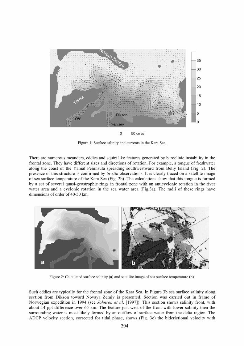
394

0

5

10

15

20

25

30

35

0 50 cm/s

Novaya Zemlya

Yamal

Dikson

Yenisey

Ob'

Figure 1: Surface salinity and currents in the Kara Sea.

There are numerous meanders, eddies and squirt like features generated by baroclinic instability in thefrontal zone. They have different sizes and directions of rotation. For example, a tongue of freshwateralong the coast of the Yamal Peninsula spreading southwestward from Beliy Island (Fig. 2). Thepresence of this structure is confirmed by in-situ observations. It is clearly traced on a satellite imageof sea surface temperature of the Kara Sea (Fig. 2b). The calculations show that this tongue is formedby a set of several quasi-geostrophic rings in frontal zone with an anticyclonic rotation in the riverwater area and a cyclonic rotation in the sea water area (Fig.3a). The radii of these rings havedimensions of order of 40-50 km.

a bb

Figure 2: Calculated surface salinity (a) and satellite image of sea surface temperature (b).

Such eddies are typically for the frontal zone of the Kara Sea. In Figure 3b sea surface salinity alongsection from Dikson toward Novaya Zemly is presented. Section was carried out in frame ofNorwegian expedition in 1994 (see Johnson et al. [1997]). This section shows salinity front, withabout 14 ppt difference over 65 km. The feature just west of the front with lower salinity then thesurrounding water is most likely formed by an outflow of surface water from the delta region. TheADCP velocity section, corrected for tidal phase, shows (Fig. 3c) the biderictional velocity with

395

almost clear anticyclonic character. The size of this eddy with the brackish core is equal 54 km. Sucheddy contains about 10 km3 river water or about one day of river flux. These anticyclonic eddies canmigrate off ROFI, transporting large quantities of river water to the ocean currents in the deeper basin.

Sal

inity

(pp

t)

35

30

25

20

15

1060 65 70 75 80

Longitude

50

25

0

-25

-50S

peed

(cm

/s)

Longitude65.5 66 66.5 67

Sal

inity

(pp

t)

30

25

20

15

10

VS

a

b

c

Figure 3: Calculated surface currents (a), sea surface salinity along section (b) and surface salinity and currentspeed normal to the ship’s track on passage through the anticyclonic structure (c).

One of the most important reasons of the pycnocline gradients changing, vertical diapicnal mixing andentrainment processes is the breaking of the internal waves. Analysis of the all available data of multi-hour and multi-day CTD stations in the Kara Sea shows the pronounced amplification of the watertemperature and salinity oscillations in pycnocline with periods from 3 hour to inertial (see Pavlov etal. [1996]). Observations of the summer surveys 1997 and 2001 demonstrated well-pronounced high-frequency internal waves with periods from 2 to 15 minutes at the background of the more long-periodic oscillations (see Stanovoy and Shmelkov [2002]). Amplitudes of the internal waves in theKara Sea can reach several meters and the changing of salinity can reach 15 units per several hoursand 0.3-0.5 (in estuaries – up to 6-8) per 10 minutes. In the coastal zone of the Kara Sea the nonlinearinternal waves were observed. But all estimations of the internal waves breaking probability werebased on the approximated estimations of the current shear or on the modeling results.

Only in summer 1995 two stations with ADCP were deployed within the frontal zone for two weeks.Analysis of the obtained records has shown the predominance of the oscillations with tidal period atthe all horizons. In Figure 4a the vertical distributions of the salinity in one ADCP station at themoments of deployment and recovery and the standard deviation of meridional current component arepresented. Also the spectra of the meridional current component oscillations at the different horizonsof this station are presented (Fig. 4b). The amplification of the oscillations in the pycnocline is shownwell. These oscillations are twice as much the barotropic tidal current. The increasing of the inertialoscillations at the second half of record period results in shear instability of the internal waves(Richarson number was less than 0.25) and increasing of entrainment. As sequent, the changing ofvertical salinity distribution, deepening of the mixing layer boundary and strengthening of thepycnocline were observed (Fig. 4a).

396

Figure 4. Vertical distribution of the salinity and standard deviation of the meridional current component (a) andspectra of the meridional current component at the horizons 4.5, 9 and 13.5 m (b) at the ADCP station in summer1995.

4 SummaryWe describe the some processes inherent in the frontal zones of the Kara Sea. These processes arevery important for frontal zones behavior. Ob’ and Yenisey rivers tend to form frontal zones structuresunder strong topographic steering throughout spring and summer. Eddies and internal waves welldeveloped in frontal zones of the Kara Sea enhance mixing and weaken the cross-front gradients ofdifferent water properties and can transport dissolved and suspended material carried by rivers for along distance.

Acknowledgments: The work was made within the frame of the Russian-German project ‘SiberianRiver runoff’, SIRRO (BMBF and Russian authorities) and the EU-project ESTABLISH (contract No.ICA2-CT-2000-10008).

References:

Hedstrom, K.S., User’s Manual for an S-Coordinate Rutgers University Model (SCRUM). Version3.0, Institute of Marine and Coastal Sciences at Rutgers University, 116 p., 1997.

Jonson, D.R., T.A. McClimans, S. King, O. Grenness, Fresh water masses in the Kara Sea duringsummer, J. Of Mar. Syst., 12, 127-145, 1997.

McClimans, T.A., D.R. Jonson, M. Krosshavn, E.E. King, J. Carrol, and O. Grennes, Transportprocesses in the Kara Sea, J. of Geoph. Res., 105, C6, 14,121-14,139, 2000.

Pavlov, V.K., Timokhov L.A.,. Baskakov G.A.,. Kulakov M.Yu.,. Kurazhov V.K., Pavlov P.V.,Pivovarov S.V., and Stanovoy V.V., Hydrometeorological regime of the Kara, Laptev and East-Siberian Seas. Technical Memorandum APL-UW TM 1-96, 179 pp., 1996.

Stanovoy, V.V., and B.S. Shmelkov., Short-period internal waves in the Kara Sea. Berichte zur Polarand Meeresforschung, 2002 (in press).

� ��

�� !"# �$%%""& '��(�� )��

� ��

��

�� ! " #�� !�� $

�

�% ��

� ��% ��!�

�" &

� �� '�� (�� )*&+� )*+� )#+�

� � �� !� �� ! "#�� !� �� !�� )**+� ),+� ��

� � ��

- �� (��

�� "*

�

��

��

�*

#�� % ��

�� *!

� �� .� �� /�� /� �� )0+� )1+� �� 2��

03,

)4+ ��

�� '�� 5�� 6�� 7��( )8+ �� '� �� 9�� -�� /�� .�� )3+ �� /��

�� :��'6��'�� :��'6��'�� '��

�� ;�� -�� -�� (��

-�� <�� '�� /�� $ :��'��

� ��

� ��

�� :��'6��'��

��

�% �� ! " �

*

�� % �� % ��

� �� $

�� " ��% �� % ��

� " �% �� % ��

� � �� -� � ��

038

��

�% ��

��

�" � �� %

*

�� % �� %�% �! % �� #!

��

� " � ��

� � �� 5��

�� " ��

� � ��

� " � ��

��

� " ��

� �� 9�� (� �� <��

6�� :��'6��'�� $

��

�%��

��

��% ��

��" �

*

�� %��

�� % ��

� 0!

�� " � �� 5�� 6�� " ��

� �� $

��

�% ��

��

�" �

*

�� % ��

��

� =!

��

! �� "�� "#��

�� *! �� 0! �� -�� $

033

��

�% �� % ��!�

�! " ��

�

��

%��

��

��

��

�� =�� % ��

� �� /��

��

��

)*+ .�� >� �� ?�� @�A�5� �� 2�� 2�� 6�� -� 0&#$1#3B11=� *343�

)#+ C�� ;� D�� - 0#&$#&3B##4� *3,&�

)0+ A� �� 5�6� �� @�� E�� >�� @�� :�F�� *33,�

)=+ 7��'C�� 2�6� �� 6�� 5�� @ �� -�� 6 �� ?��'�� 6�� :��'E�� @�� *&$1#3B1=3� *34*�

)1+ 2�� @�@� �� 6�� 6��:�� A�� 7�� C�� D�� *383�

)4+ 2�� >� �� ! !��"��"��!�� # � �

��"�� !��!"� !�� G��H�9�� *I31� �� H�� .�� E��'��H�� C�� E��H�� C�� C�� *331�

),+ 6� �� @� 6�� 2�� :�� ;�� 5�� ?D66 38IJI=#� ?D66'�� (�� ?�� ?�� *338�

)8+ 6�� -� �� 7��(� 5�6� G�� @�� E�� 7�� @�� $�� % !� �� !� *0$11B,3� *383�

)3+ ��/�� 2�-�@� �� .�� 6�J� K� � � ;�� >��6�� =18$##3B#4,� #&&#�

)*&+ � �� ?�.� - ?�� -�� 7�� :�� ;�� E�� 7�� ##$#,0B#80� *341�

)**+ �� A� J�� :�� 5�� ?�� ,&$**0B*#4� *3,1�

=&&

401

Modeling the oceanic response to episodic wind forcingover the West Florida ShelfSTEVEN L. MOREY


MARK A. BOURASSA


XUJING JIA


JAMES J. O’BRIEN


WILLIAM W. SCHROEDER

(Marine Science Program, The University of Alabama, Dauphin Island Sea Lab, 101Bienville Blvd., Dauphin Is., AL, USA, 36528, [email protected])

JORGE ZAVALA-HIDALGO


1. IntroductionShallow seas and wide continental shelves respond dramatically to local energetic episodic windforcing, such as atmospheric fronts and tropical storms. High-resolution ocean models show greatpromise in simulating the ocean environment at these regional scales, but are often limited by theavailability of gridded wind fields for surface fluxes that have high enough spatial and temporalresolution to adequately capture these strong events. Numerical weather prediction products aretypically too coarse and the fields can be too smooth to adequately resolve these energetic systems.Winds measured by the Seawinds scatterometer aboard the Quikscat satellite have admirable qualityand spatial resolution, but the bandlike sampling can lead to large temporal gaps at some locations,which complicate the representation of moving weather systems. In this study, comparisons are madebetween results of a numerical model of the Gulf of Mexico (GoM) forced by objectively griddedsatellite scatterometer winds, Eta-29 atmospheric model forecast data, and a hybrid of the satellite andnumerical weather prediction products. Validation of the model results with in-situ observationsshows the strengths and weaknesses of using the different gridded winds for modeling the region.Particular attention is paid to episodic weather events, such as tropical systems and atmospheric fronts.The West Florida Shelf (WFS) region is chosen for the focus of this study as a testbed for examininghow best to use satellite derived winds to force regional-scale ocean models.

2. The ModelThis study evaluates the solution from simulations of the GoM using the Navy Coastal Ocean Model(NCOM). The NCOM is a three-dimensional primitive equation hydrostatic ocean model developedat the Navy Research Laboratory (see Martin [2000]). The model’s hybrid sigma (terrain following)

402

and z (geopotential) level vertical coordinate is useful for simulating upper ocean processes indomains encompassing both deep ocean basins and very shallow shelves. The NCOM is set up tosimulate the entire GoM and Caribbean north of Honduras (15° 30' N) to 80° 36' W with 1/20°between like variables on the C-grid, 20 sigma levels above 100 m and 20 z-levels below 100 m to amaximum depth of 4000 m (Figure 1). The model is forced by discharge from 30 rivers, transportthrough the open boundary (with monthly climatology temperature and salinity) yielding a meantransport through the Yucatan Strait of approximately 30 Sv, monthly climatology surface heat flux,and twelve-hourly winds. A surface salinity flux has the effect of uniformly evaporating an amount ofwater at a rate equal to the sum of the annual average discharge rates of the 30 rivers. The model isspun up from rest using DaSilva monthly climatology wind stress for approximately five and one-halfyears before the twelve-hourly wind stresses are applied.

Figure 1: Left: NCOM GoM simulation domain and topography. Right: Bathymetric chart of the WFS region(shown by the white box to the left) with the locations of the in situ data used for model validation.

3. The Wind FieldsThree gridded wind products are used to force the ocean model: the 29 km resolution Eta-29 model 10m winds, winds derived from the SeaWinds scatterometer aboard the QuikSCAT satellite objectivelymapped to a 1/2° grid using winds from the same scatterometer data to create a background field, andanother mapping of the QuikSCAT winds using the Eta-29 winds as the background field (these threewind fields will be termed ETA, QSCAT, and QSCAT/ETA, respectively, for convenience). Windstress fields are prepared to force the ocean model from July 21, 1999 through the end of 2000. Thestarting date corresponds to the beginning of the QuikSCAT observations.

To form the two gridded scatterometer wind products, the pseudostress is objectively gridded usingthe variational method described by Pegion et al. [2000]. The functional

f P P P P L P P L P P L k P Pa P x x y y d x x d y y e bgi j

I J

o o o bg bg= −( ) − −( )

+ ∇ −( )

+ ∇ −( )

+ ⋅∇ × −( )[ ]

−∑ β σ β β β2 2 2 4 22

4 22

2 2r r

,

,

is minimized for the solution pseudostress (Px, Py). Here, the terms with the small ’o’ subscripts arethe observations from the satellite, and the terms with the small ’bg’ subscripts are the backgroundfield. The betas are weights, sigma is the uncertainty of the observational average within a grid cell,and L is a grid-spacing dependent dimensionless length scale. The first term represents the misfits tothe scatterometer observations, the second and third terms comprise a penalty function to smooth withrespect to the background field, and the last term is the misfit to the vorticity of the background field.

COMPS ADCP

Naples (NPL)

Clearwater Beach (CWB)

Cedar Key (CDK)

Apalachicola (APA)

403

For the QSCAT gridded wind product, the background field is constructed from 3-day binnedQuikSCAT wind data, Gaussian smoothed over a five degree radius. For the QSCAT/ETA product,the background field is the Eta-29 wind field.

Observations collected within a twelve-hour window centered on 0:00Z or 12:00Z are treated as theobservations at the middle of the time window. Therefore, twelve hourly gridded wind pseudostressfields are produced. For consistency, the Eta-29 wind fields from the same twice-daily times areselected for the model experiments. The wind stress is computed from the bulk formula with the dragcoefficients computed using a quadratic function of the wind speed. The resultant wind stress isinterpolated to the ocean model grid using bicubic splines.

4. ResultsThe ocean model solutions are compared to data collected over the WFS. The WFS is chosen as atestbed for evaluating the impact of the different wind stress fields as forcing for coastal and regionalscale ocean models because it has been shown that the circulation on the inner and middle WFS isprimarily driven by local winds (See Weisberg, et al. [2001]). The region is also subject to episodicenergetic forcing from tropical and extratropical storms. It is useful to study the response of the oceanmodel forced by the various wind products during these periods of energetic forcing. Data arecollected from coastal sea level (SL) stations and from a moored acoustic doppler current profilerdeployed as part of the Coastal Ocean Monitoring and Prediction program at the University of SouthFlorida. Only the SL comparisons will be discussed here.

SL time series from the NCOM experiments are compared to in situ data at four stations along theWFS: Naples, Clearwater Beach, Cedar Key, and Apalachicocla (Figure 1). The observational andmodel data are filtered to form sets of daily SL values. SL root mean square error (RMSE) scaled bythe standard deviation (of the observational data computed over same time record used for computingRMSE) is used as one metric for evaluating the model performance. SL can be thought of as afunction of the wind stress (alongshore) integrated along the characteristics of the coastally trappedwaves, propagating counterclockwise around the GoM. The Florida Keys to the south of the shelfserve approximately as an insulating boundary.

The results are similar for all stations studied; Cedar Key is used as an example here. The standarddeviation of the observations is 13.1 cm for the full time record studied at this location. The scaledRMSEs are 0.88, 0.75, and 0.73 for the simulations forced by ETA, QSCAT, and QSCAT/ETA,respectively. To study the different behavior of the ocean model response to energetic wind forcingversus the more typical conditions, the time record is decomposed into two parts. The first consists ofall data within a 7-day window centered around any day with observed SL fluctuations greater thantwo standard deviations (26.2 cm, in this case) of the mean. This record comprises approximately20% of the data. Most of this subset of data is from the late fall through early spring months whenthere are frequent passages of cold fronts through the region, with occasional tropical cyclones (threepassed during this period) during the summer and early fall months. The second part of thedecomposed record consists of the remaining data, and contains more moderate or weak SLfluctuations. The results show that during weak or moderate events the simulations perform similarlywith scaled (now by a standard deviation of 9.5 cm) RMSEs of 0.91, 0.92, and 0.91 corresponding tothe ETA, QSCAT, and QSCAT/ETA forced simulations, respectively. However, during the part ofthe record corresponding to energetic SL fluctuations (and, thus, more energetic forcing), thesimulations forced by the scatterometer derived gridded wind products perform much better. Scaled(by a standard deviation of 20.2 cm) RMSEs are 0.88, 0.62, and 0.60 for the simulations as orderedabove. That is, using this metric, the model solution shows significant improvement when the QSCATand QSCAT/ETA gridded wind stress fields are used during periods of energetic wind forcing,however, the model performance is similar under all conditions when forced by the ETA wind stressfields.

404

5. DiscussionThe large errors in the model solution when forced by the ETA wind stress fields are primarily due tothe fact that the ETA wind fields are smooth and weak, a trait often found in numerical weatherprediction products. The scatterometer observations are better able to represent the intensity andspatial patterns of energetic weather systems. Comparisons of the wind stress from the griddedproducts to the wind stress computed from National Data Buoy Center measurements show that theaverage ETA wind stress is approximately 50% of the magnitude of the observations, whereas thescatterometer derived wind stress fields have quite similar magnitudes to the observations in thisregion. It is not clear, however, whether simply multiplying the ETA wind stress vectors by a scalar isan appropriate solution, as the spatial structure of QSCAT and QSCAT/ETA fields is often quitedifferent from the ETA fields. An example from each of the three fields during the passage ofTropical Storm Harvey illustrates this fact (Figure 2).

Figure 2: Wind stress (Pa) fields from the gridded ETA (left), QSCAT (middle) and QSCAT/ETA (right) windstress fields on September 20, 1999, just prior to T.S. Harvey passing eastward over the WFS.

Acknowledgments: The authors thank Drs. Paul Martin, Alan Wallcraft, and others at the Navy ResearchLaboratory for their development of and assistance with the Navy Coastal Ocean Model. Drs. Robert Weisbergand Mark Luther at the University of South Florida graciously provided the COMPS ADCP data. Simulationswere performed on the IBM SPs at Florida State University and the Naval Oceanographic Office. Computertime was provided by the DoD High Performance Computing Modernization Office. This project was sponsoredby funding provided by the DoD Distributed Marine Environment Forecast System, by the Office of NavalResearch Secretary of the Navy grant awarded to Dr. James J. O'Brien, by a NASA Office of Earth Science grantto the COAPS authors and through NASA funding for the Ocean Vector wind Science Team. Frank Wentz atRemote Sensing Systems produced the scatterometer data.

References:

Martin, P., A description of the Navy Coastal Ocean Model Version 1.0. NRL Report NRL/FR/7322-009962, Naval Research Laboratory, Stennis Space Center, MS, 39 pp., 2000.

Pegion, P.J., M.A. Bourassa, D.M. Legler, and J.J. O'Brien, Objectively derived daily "winds" fromsatellite scatterometer data. Mon. Wea. Rev.,128, 3150-3168, 2000.

Weisberg, R.H., Z.J. Li, and F. Muller-Karger, West Florida Shelf response to local wind forcing:April 1998, J. Geophys. Res., 106, 13239-262, 2001.

405

Transport over a Narrow Shelf: Exuma Cays, BahamasNED P. SMITH

(Harbor Branch Oceanographic Institution, Fort Pierce, Florida 34946, U.S.A.,[email protected])

1. IntroductionThe Exuma Cays separate the western side of Exuma Sound from the eastern margin of Great BahamaBank (Fig. 1). The cays extend 130 km from Norman Cay (24o 39.3'N, southeast to Rat Cay (23o

44.2’N) at the northern end of Great Exuma Island. Thirty major tidal channels and numerous smallerchannels, exchange significant amounts of water between the sound and the bank. For example, atpeak flood and ebb, current speeds through Adderley Cut, at the northern end of Lee Stocking Island,reach 80-100 cm s-1 (Smith 1996), and transport commonly reaches 1000-1500 m3 s-1. Cumulativehalf tidal cycle flood and ebb volumes average 16.3 and –26.1 x 106 m3, respectively.

Fig. 1. Map of study area off the northern end of Lee Stocking Island, Exuma Cays, Bahamas. C shows thelocation of the current meter. The AC arrow points to the mouth of Adderley Cut, which connects shelf waters of

Exuma Sound with the shallow waters of Great Bahama Bank.

The continental shelf on the Exuma Sound side of the Exuma Cays is generally between 1 and 2 kmwide, and the shelf break is the top of a “wall,” at a depth of 25-30 m. Water depth increases abruptlyto approximately 200 m, and from the base of the wall the slope of the sea floor is approximately 60o.Water depths of 1000 m occur within just a few kilometers of the Exuma Cays. Because of the narrowwidth, across-shelf transport occurs over unusually short time scales. For example, Stoner and Smith(1997) showed that the location of highest concentrations of larvae in surface layers across the shelfcorrelated most highly with wind stress over the preceding 6-8 hours.

Shelf circulation is responsive to wind forcing, but coherence is reduced because of the vigorous tidalexchanges. Ebb tide plumes can extend across the entire shelf and interrupt the wind-driven along-shelf movement of water. Near-bottom current observations from the outer shelf directly seaward ofthe mouth of Adderley Cut have across-shelf components at tidal periodicities that are commonlybetween -5 (shoreward) and +20 cm s-1 (Smith 1996). Even as ebb tide plumes perturb along-shelfwind-driven transport, however, they also serve to enhance across-shelf turbulent transport asmesoscale eddies are generated by alternating landward and seaward deflections. This paper focuseson the across-shelf transport of heat and momentum by turbulent transport over time scales rangingfrom a few hours to a few days.

406

2. DataCurrent meter data were recorded hourly for 402 days at an outer shelf study site off the northern endof Lee Stocking Island (Fig. 1). A General Oceanics Mark II current meter was moored 13 m abovethe bottom in 22 m of water from October 22, 1991 to November 27, 1992. Speed and directionaccuracies are ±1 cm s-1 and ±2o, respectively. Bursts of 8 samples taken every 2 seconds were vector-averaged to reduce high-frequency noise in the data. Water temperature was recorded by the currentmeter with an accuracy of ±0.25o C.

Wind speed and direction, air temperature and humidity were measured at a study site at the northernend of Lee Stocking Island, 300 m from the coast on the Exuma Sound side of the island andapproximately 1 km from the current meter. Wind was recorded 3 m above the surface, andtemperature and humidity were recorded 2 m above the surface. The weather station is on thesouthwest side of a landing strip, and there are no nearby topographic features when winds are out ofthe northern and eastern quadrants (landward). Weather variables were recorded hourly from July 7through November 27, 1991. During this 143-day time period, winds were landward 81% of the time.

3. MethodsWater temperatures are combined with across-shelf current components to track the across-shelftransport of heat, and along-shelf (v) and across-shelf (u) current components are used to quantifyacross-shelf momentum transport. Current and temperature data are high-pass filtered to focus onmeso-scale turbulence generated by semidiurnal tidal exchanges, and perturbation analysis is used toinvestigate across-shelf transport of heat and momentum over time scales ranging from hours toseasons. Perturbation quantities for the ith observation of the across- and along-shelf componentcurrent speed and water temperature (t) are defined by

ui’ = ui – Ui, vi’ = vi – Vi and ti’ = ti – Ti,

where the prime notation refers to the high-frequency deviations of the hourly observation (ui, vi andti) from the low-pass filtered value (Ui, Vi and Ti) (Bloomfield, 1976). With this filter, 90% of theinput variance is retained at a period of 30 hours, 50% at 37 hours and 10% at a period of 48 hours.To focus on the longer-term effects of tide-induced across-shelf transport, perturbation products areaccumulated. Thus, for hours 1 through m of the time series, the cumulative heat flux, Fh, is given by

and the cumulative momentum flux is

Quadratic wind stress was quantified using the drag coefficient suggested by Wu (1980). Air densitywas calculated using the virtual temperature, but no adjustment was made to approximate a 10-m levelover-water wind speed.

,''1∑ =

= m

ih tuF

.''1∑ =

= m

im vuF

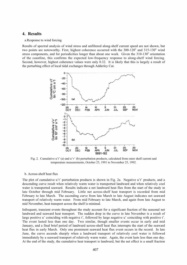
407

4. Resultsa.Response to wind forcing

Results of spectral analysis of wind stress and unfiltered along-shelf current speed are not shown, buttwo points are noteworthy. First, highest coherence occurred with the 300-120o and 315-130o windstress components, and for periodicities longer than about one week. Given the 310-130o orientationof the coastline, this confirms the expected low-frequency response to along-shelf wind forcing.Second, however, highest coherence values were only 0.32. It is likely that this is largely a result ofthe perturbing effect of local tidal exchanges through Adderley Cut.

Fig. 2. Cumulative u’t’ (a) and u’v’ (b) perturbation products, calculated from outer shelf current andtemperature measurements, October 25, 1991 to November 25, 1992.

b. Across-shelf heat flux

The plot of cumulative u’t’ perturbation products is shown in Fig. 2a. Negative u’t’ products, and adescending curve result when relatively warm water is transported landward and when relatively coolwater is transported seaward. Results indicate a net landward heat flux from the start of the study inlate October through mid February. Little net across-shelf heat transport is recorded from midFebruary to late March. The ascending curve from late March to late August indicates net seawardtransport of relatively warm water. From mid February to late March, and again from late August tomid November, heat transport across the shelf is minimal.

Infrequent, transient events throughout the study account for a significant fraction of the seasonal netlandward and seaward heat transport. The sudden drop in the curve in late November is a result oflarge positive u’ coinciding with negative t’, followed by large negative u’ coinciding with positive t’.The event lasted less than one day. Two similar, though smaller events occur in early and midJanuary, and a final brief period of landward across-shelf heat flux interrupts the start of the seawardheat flux in early March. Only one prominent seaward heat flux event occurs in the record. In lateJune, the curve ascends sharply when a landward transport of relatively cool water is followedimmediately by a seaward transport of relatively warm water. Again, the event lasts less than one day.At the end of the study, the cumulative heat transport is landward, but the net effect is a small fraction

408

of the landward transport during fall and early winter, or the seaward transport during spring and earlysummer.

c. Across-shelf momentum flux

The plot of cumulative u’v’ perturbation products is shown in Fig. 2b. Negative perturbation productsoccur when ∆v’/∆x > 0, e.g., when positive v’ perturbations increase seaward, or when negative v’perturbations decrease seaward. From the start of the record through mid April the curve descendsirregularly. Most of the decrease occurs before mid January and from late March through the first halfof April. The ascending curve from mid April to late October is produced by ∆v’/∆x < 0, viz., somecombination of positive v’ perturbations decreasing seaward and negative v’ perturbations increasingseaward. Taken together, these two components of Fig. 2b suggest, that ∆v’/∆x reverses at about thesame time the across-shelf temperature gradient reverses. Relatively weak positive v’ perturbations(or relatively strong negative v’ perturbations) move seaward from the inner shelf during fall andwinter, when warm water is imported onto the inner shelf. Then relatively strong positive v’perturbations (or relatively weak negative v’ perturbations) move seaward during spring and summer,when heat is being exported from the inner shelf.

References:

Bloomfield, P. 1976. Fourier Analysis of Time Series: An Introduction. John Wiley & Sons. NewYork. 258 pp.

Smith, N.P. 1996. The effect of hyperpycnal water on tidal exchange. Pp. 107-116 in: BuoyancyEffects on Coastal and Estuarine Dynamics (D. Aubrey and C. Friedrichs, eds.). Coastal and EstuarineStudies, vol. 53. American Geophysical Union, Washington, D.C.

Stoner, A.W. and N.P.Smith. 1997. Across-shelf transport of gastropod larvae in the centralBahamas: rapid response to local wind conditions. J. Plankton Res. 20:1-16.

Wu, J. 1980. Wind-stress coefficients over sea surface near neutral conditions—a revisit. Journal ofPhysical Oceanography 10:727-740.

409

Modelling flow, water column structure and seasonality inthe Rockall SlopeALEJANDRO J. SOUZA

1, SARAH WALKELIN1, JASON T. HOLT

1, ROGER PROCTOR1 AND MIKE

ASHWORTH2

1Proudman Oceanographic Laboratory, Bidston Observatory, Bidston Hill, Prenton CH437RA, UK2CLRC, Daresbury Laboratory, Warrington, WA4 4AD, UK

1. IntroductionThe accurate simulation of currents, water quality parameters and plankton variability in shelf seasrequires a physical model that includes the effects of vertical and horizontal density variations. This isnecessary since the former introduces horizontal transports while the latter controls vertical fluxescritical for biological production (Holt and James, 2001). Furthermore, shelf sea fronts (both thermaland haline) affect both the horizontal and vertical transfer of momentum and tracers. To accuratelymodel this we need the development of fine resolution 3-dimensional hydrodynamic models.

This is why the Proudman Oceanographic Laboratory Coastal Ocean modelling system (POLCOMS)has been developed to tackle multidisciplinary studies in the coast/shelf and shelf edge environments(figure 1).

The central core is a sophisticated 3-dimensional hydrodynamic model that provides realistic physicalforcing to interact with, and transport, environmental parameters. Integrating from ocean to coast andvice versa, biological production and the fate of contaminants can be determined.

The objective of this work is to show a fine resolution application of POLCOMS to the Rockall shelf-edge region and to show that the model has been successful in reproducing the dynamics of this area.

2. The hydrodynamic modelThe hydrodynamic model is a 3-dimensional model with temperature and salinity treated as prognosticvariables, developed at the Proudman Oceanographic Laboratory using an Arakawa B-griddiscretisation. The original model was produced by James (1986) and has subsequently beingdeveloped to include, the Piecewise Parabolic Method (PPM), non-diffusive advection scheme (James,1996). The advantage of having a non-diffusive B-grid model for shelf seas is that the B-gridprevents the dispersion of velocity features associated with fronts and the PPM advection schemeavoids diffusion of momentum and scalars making it an ideal tool to model typical baroclinic shelffeatures such as river plumes (James, 1997) and fronts (Proctor and James, 1996). These twocharacteristics are what particularly distinguish the model

410

Figure 1. The POLCOMS paradigm

from other shelf sea model such as the Princeton Ocean Model (POM) (Blumberg and Mellor,1987).

The model is formulated in spherical polar sigma coordinates: λ (eastward), φ (northward) and σ(vertical), with σ = ( z - ζ )/( h + ζ ), where z is the Cartesian vertical coordinate, h is the water depthrelative to the reference sea level ( z = 0 ) and ζ is the elevation above this.

The incompressible, hydrostatic, Boussinesq equations of motion are solved using time splittingbetween barotropic and baroclinic components. Baroclinic pressure gradients are computed onhorizontal planes with spline interpolation through the vertical σ grid point distribution. Verticalmixing is parameterised using the Mellor-Yamada 2.5 turbulence closure scheme. Horizontal diffusionof momentum and scalars can be included with a linear or shear-dependent (Smagorinsky form)coefficient of diffusion. For detail explanation of the model see Holt and James (2001).

3. Model applicationThis particular application uses a horizontal resolution of 1 nautical mile with 34 S-levels. It attemptsthe most realistic simulation possible, so it uses realistic meteorological forcing supplied by the UKmet-offices and the initial and lateral boundary conditions are provided from a 12 km shelf-wideversion of POLCOMS, which is it self forced by the UK Met-office FOAM.

411

Figure 2. Example model output showing bottom (left) and surface (right) temperature and currents, velocityvectors show only a fifth of the model resolution.

4. Model ResultsThe preliminary results show consistency with previous observations in the Roackall shelf-edge(Souza et al, 2001), with a warm Northward slope current of about 20 cms1 with strong variability dueto eddies. The eddy field reproduced by the model resembles that observed by satellite imagery (figure2). The model also reproduces the seasonal variability shown by the UK Shelf Edge Study (Souza etal, 2001).

References.

Blumberg, A.F. and G.L. Mellor (1987). A description of a three-dimensional coastal ocean model. Inthree Dimensional Coastal Ocean Models, Coastal and Estuarine Studies, vol4, edited by N.S. Heaps,pp1-16, AGU, Washington, D.C.

Holt, J.T. and James, I.D. (2001) An S coordinate density evolving model of the northwest Europeanshelf 1, Model description and density structure. Journal of Geophysical Research, 106, C7, 14015-14034.

James, I.D. (1986). A front-resolving sigma coordinate model with a simple hybrid advection scheme.Appl. Math. Modell., 10, 87-92.

James, I.D. (1996). Advection schemes for shelf se model. J. Mar. Sys., 8 237-254.

James, I.D. (1997). A numerical model of the development of anticyclonic circulation in a gulf-typeregion of freshwater influence. Cont. Shelf Res.,17, 1803-1816.

412

Patsch, J. and Radach, G. (1997). Long-term simulation of the eutrophication of the North Sea:temporal development of nutrients, chlorophyll and primary production in comparison to observations.J. Sea Res., 38 (3/4) 275-310.

Proctor, R. and I.D. James (1996). A fine-resolution 3-D model of the southern North Sea. J. Mar.Sys., 8, 285-295.

Souza, A.J., J.H. Simpson, M. Harikrishnan and J. Malarkey (2001). Flow structure and seasonality inthe Hebridean Slope Current. Oceanologica Acta,24, S63-S76.

��

��

�� !� ��"� #��$��%��& '� (��)�* !� ��"� +� �� ,�� -�� .�� & �)� (�

�/��* ��0� +� ��

� ��

�� !�� ! �"�� #� �� $ %� �� &�� &��!�� '(�� '�� (�� !�� )�**�+$

,�� -�� $ ,�� .�� !�� -�" �� $

� ��

�� !�� &�� $ / �� 01�2� �� .�� * 3�$ �� !�� !�� 4�� 1$

�� 5� !�� 21� � �� 26� � �� ! �� $

� ��

7�� #� !�� 8�� "9��$ ,�� .�� .�� !� '(�� .�� $ &�� !�� 5�� :�� !�� $ '(�� 9�� $�$ ;<��=(�� ;<(=7(( �� $ �� !�� '(�� '�� '�� !�� !�� $ /� �� 39� ��!�� $

,�� 1> ;�� !�� !�� $

� � ��

�� 4� �� 4�� $ �� !�� 8�� "�� $ ��!�� 4�� 4��$ �� ;<(=7((�� ;<��=(�� !�� #*? �� 3 ��4��$ �� "�� ! �� @ ��3� �� !�� $ /�� 4�� &�� '(��9�;<(=7(( �� $

�� !� �� 4��#$ �� '(�� &�� "�� *$2 :$ �� "�� $ �� 8�� !�� -�� $ �� * � �� * � �� !��$ 7�� !�� !�� "�� $ ;�� 4�� $ ,�� !�� '(�� !�� 4�� ! �� !�� $

�� 4�� 0A � �� 4�� @$ / �� !� �� "�� &�� "��

,�� > <�� $ &�� 9 �� '(��9;<��=(�� 9 !��3 �� '(��9�;<(=7(( 9 �� $

,�� #> &�� "�� $�� !�� * �� * � � ��!��$

,�� @> �� 4�� 4�� $

'(�� "�� $ �� 4�� '(�� !�� !�� $ �� ! �� !�� !�� '(�� !�� '(��9;<��=(�� $

� ��

�� !�� !�� '(�� &�� 8�� !�� !�� $

&�� .�� !�� 4�� $ �� !�� 4�� $

�� ! ��

��

� � � � ��

7�� &$� �� :$ 7�� '(�� $ ��4��$ ��$ =��$ (;= �*�2# (�� (�� 5�� 126 ��$� �**�$

417

Sediment Flocculation and Flow in a Tidal MarshEnvironment.GEORGE VOULGARIS

(Marine Science Program, Department of Geological Sciences, University of South Carolina,Columbia, SC 29208, USA, [email protected])

SAMUEL T. MEYERS

(Marine Science Program, University of South Carolina, Columbia, SC 29208, USA,[email protected])

1. IntroductionSalt marshes are invaluable ecological resources along the Southeast coast of the United States. Thesurvival of these resources is dependant on their ability to import and accumulate sediment at a ratesufficient to keep pace with the regional rise in sea level. Sediment erosion, transport and deposition inthese environments are important from both geomorphological and geochemical points of view. Whilethe morphology reflects the age, maturity and tidal characterstics of the marsh, the sedimentcharacteristics (i.e., size, concentration, properties) affect the ability for chemical pollutants to betransported and accumulate in the marsh. The traditional theory for sedimentation in the intertidal zoneis that of settling and scour lag effects that assume a single particle size that remains constant throughthe tidal cycle. In this study the variability in particle size as a function of flow strength is examinedand the implications in sediment transport are discussed.

2. BackgroundSuspended sediment in estuaries is predominantly found in flocculated form (Van Leussen 1997). Thecoalescence of charged clay particles occurs in saline water when numerous cations are free to interactwith the particles. Mucous biofilms from algae, bacteria and higher plants also cause the aggregationof particles to occur upon collision with other particles. This process of flocculation has a significanteffect on the behavior of particles in suspension that varies from the behavior of their constituentparticles. Flocculated particles will continue to increase in size as particle collision continues, due tosettling or turbulent mixing, until shear becomes strong enough to prevent aggregation or causedisaggregation. Increased turbulence will often promote flocculation at first through particle-to-particle collision, but then reaches a critical level when the flocs can no longer retain their shape andstart to break apart (Van Leussen 1997). The ability to define these critical levels offers a betterunderstanding and prediction capability of the mode by which sediment is transported throughoutvarious stages of the tidal cycle

3. LocationVelocity and suspended sediment concentrations were collected during three deployments at a locationin the upper region of Bly Creek, a terminal tidal creek basin comprising a portion of the North Inletsalt marsh near Georgetown, South Carolina (USA). The North Inlet marsh is a back-barrierenvironment composed of meandering channels with an approximate area of 32 km2. The primaryexchange of water in the marsh is with the Atlantic Ocean through North Inlet to the east with verylittle fresh water influence from the neighboring uplands and Winyah Bay estuary to the south. Themarsh has astronomical tides that are semidiurnal with an average range of 1.4 m and has a slightdiurnal inequality. The Bly Creek basin is ebb-dominant with a well-developed channel and steepbanks. The dominant vegetation in the marsh is Spartina Alterniflora, which covers the entire marshsurface above the creek banks, with small patches of Juncus in the high marsh. The surface sediment

418

of the vegetated marsh is composed primarily of silt while the channel beds are composed of silt andsand.

4. MethodsExperiments were performed to define the relationship between turbulence, flocculation, particle sizedistributions, and suspended sediment characteristics. A 10 MHz Sontek acoustic Doppler velocimeter(ADV) measured 3-D velocities at a single point and was used to calculate the turbulent characteristicsof flow. An optical backscatter (OBS) turbidity sensor was mounted in-sync with the velocimeter tomeasure the total suspended sediment concentration, while a laser particle size analyzer (LISST) wasused to measure the size distribution in the range of 1.25-250 um. A hand-powered bilge pump wasalso used to collect water samples that were filtered and weighed for total suspended sedimentconcentration. A galvanized steel frame supported the instrumentation and was placed in the thalwegof the channel. The sample volumes for the instruments and pump were 15 cm above the bed. TheADV, OBS, and LISST were programmed to sample continuously for 12 minutes every half hourranging from 2 to 8 days. The third deployment captured the longest time series and was the onlydeployment in which all of the instruments collected valid data simultaneously.

5. ResultsFriction velocity was calculated using the covariance method, turbulent kinetic energy method, andinertial dissipation method. Similarity of all three values established the accuracy of the estimates. Amean of the three friction velocity estimates was calculated and used for data analysis. Results showthat as the mean current flow and friction velocity increase flocs size increase. The effective densityand settling velocity of the flocs were found to be in agreement with published data, from the oceanenvironment (Dyer and Manning 1999, Manning and Dyer 1999, Mikkelson and Pejrup 2001).Effective density of the flocs decreased with increasing floc size while the settling velocity increasedwith floc size (Fig. 1). By calculating the Kolmogorov microscale (η), the upper limit on floc size canbe estimated. While the limit of floc growth was never surpassed during the third deployment,measurements from the OBS during the second deployment imply that the limit was surpassed and theflocs actually may have begun to disaggregate. Unfortunately, no LISST data from the seconddeployment was retrieved to confirm this notion. Fresh water discharge was neglogible during theexperiments thus all results are attributed to changes in turbulence levels rather to changes in watersalinity

Figure 1. Effective density (∆ρ) and fall velosity (Ws) of suspended sediment vs mean grain size, Dm (left andright panels, respectively) from this study compared with the results from Mikkelson and Perjup (M&P, 2001)

419

Figure 2. Effective settling velocities (mm s-1) of suspended sediment estimated assuming various fractaldimensions vs. mean grain size Dm. Fractal dimensions (nf) from 3 (spheres) to 2 are plotted in order to observe

the change in settling velocity due to decreased diameters.

Various fractal dimensions (nf) were applied to the LISST data to determine the effect of particlegeometry on settling velocity. Results show that the settling velocity of most of the flocs in suspensiondoes not change with different values of nf, indicating that in similar environments, the settlingvelocity is not sensitive to the true shape of the flocs. As the fractal dimension decreases, the effectivedensity of the particles must increase. As larger flocs usually have greater settling velocities thansmaller flocs, the increase in density with smaller fractal dimensions balances this change in floc sizeand no great variation in settling velocity is revealed (Fig. 2). Since problems may arise when theLISST assumes all particles are spherical, it is important to determine the effects this has on actualparticle density and settling velocities.

The results of testing various fractal dimensions on flocculated particles reveal that the LISSTprovides very good estimates for the parameters concerned. However, this only holds true forflocculated particles (Mikkelson and Pejrup 2001) and within turbulent regimes that do not surpass thefloc growth limit. As soon as shear stress increases to the level of particle disaggregation, the aboverelationship is no longer valid.

6. ConclusionsAccurate estimates of friction velocities using the covariance, turbulent kinetic energy, and inertialdissipation methods combined with particle size and concentrations of sediment in suspension enabledus to relate flow with sediment dynamics in a tidal creek environment. It was found that:

� Increased velocity and turbulence cause increases in particle size through the process of focculationwhile still within the limits of the Kolmogorov scale.

� As floc size increases, effective density was shown to decrease while settling velocity increased.

420

� As the fractal dimension of particles changes, there was little variation in the settling velocity offocculated sediment. This confirms the ability of the LISST to provide good estimates of thevolume concentration of suspended sediment in similar environments.

In the final paper we will present some numerical results indicating the implication of the floculationprocesses in salt marsh sedimentation processes.

Acknowledgments: The authors would like to acknowledge Belle W Baruch Institute for Marine Biology andCoastal Research for providing access to the site. Funding for this work was provided through a University ofSouth Carolina Research and Productive Scholarship awarded to G. Voulgaris. Additional funding was providedto S. Meyers through a John Hodge Summer Research Fellowship.

References:

Dyer, K.R., and Manning, A.J., Observation of the size, settling velocity and effective density of flocsand their fractal dimensions. Journal of Sea Research, 41, 87-95, 1999.

Manning, A.J., and Dyer, K.R., A laboratory examination of floc characteristics with regard toturbulent shearing. Marine Geology, 160, 147-170, 1999.

Mikkelson, O., and M. Pejrup., The use of a LISST-100 in-situ laser particle sizer for in situ estimatesof floc size, density and settling velocity. Geo-Marine Letters, 20, 187-195, 2001.

Van Leussen, W., The Kolmogorov microscale as a limiting value for the floc sizes of suspended fine-grained sediments in estuaries. In: Burt, N., Parker, R., Watts, J. (eds), Cohesive Sediments. JohnWiley & Sons Ltd., pp.45-62, 1997.

421

GIS-Based Sediment Transport Study in Kyunggi Bay,KoreaCHANG S. KIM, HAK SOO LIM, SUE HYUN LEE, SUN JEONG KIM, JONG-CHAN LEE

(COASTAL ENGINEERING DIV, KOREA OCEAN R&D INSTITUTE 1270 SA 1 DONG ANSAN 425-744SOUTH KOREA , [email protected])

1. IntroductionThe Kyunggi Bay (125-128E, 36-38N) is a macro-tidal bay in the western central port of KoreanPeninsula (Fig.1). The Bay characterizes its feature as wide tidal flats, deep tidal channels and tidalsand ridges running in parallel to tidal flows. The macro-tidal range (up to approximately 8.6m) andconsequent strong tidal currents erode the bottom sediment and selectively transport to the low-energyarea forming tidal ridges or tidal flats.

The tides in the Bay are mostly of semi-diurnal types with increasing tidal range toward the shoreline.The main flows of flood direct toward north-east while the ebb currents flow south-westward.Relatively strong currents occur along the spatially distributed channels, implying spatialnonhomogeneity in sediment characteristics.

Figure 1: Study area map ; the bathymetry was reproduced by using the digital navigation chart.

2. MotivationDue to the public awareness and fishermen�s interest, the potential environmental impacts of underseasand mining has been drawn attention. The motivation of the study is how we could balance thepositive and negative impacts arising from the undersea sand mining in the Bay.

3. Goals of the studyThe goals of the study is to quantity the sediment transport processes due to the undersea sand mining,to predict the recovering processes of the sand pits, and to provide time-varying distributions ofenvironmental parameters in the GIS system that is coupled with ecological impact assessment.

422

4. Field Observation and Estimation of Co.A prototype field experiment has been conducted in an undisturbed area where the sediment types arefavored by dredging company. The purpose of setting the test site is to measure the majorhydrodynamic and sediment parameters affected by the mining operations, and their progressivevariation in time and space, including the dispersion of surface benthic plumes, and the recovery statusof the pit in the seabed. Through the filed experiment, the sediment flux (source concentration at thesource cell) and the sediment size has been measured for modeling control parameters. The temporalvariation of the mining pit has been observed to estimate the recovering rate of the disturbed seabed.

Figure 2: Observed concentration profiles of suspended materials sampled at different points away from themining site.

0

2 0

4 0

6 0

8 0

100

0 2 0 4 0 6 0 8 0 100

NTU

PPM

Figure 3: Comparison of directly sampled concentration(PPM) and YSI measured concentration(NTU) :y=0.2987+1.2317x, R2=0.997.

5. Mathematical ModellingThe Mathematical description of the physical and sediment transport processes are performed bymeans of 1-D, 2-D and 3-D models. The 1-D model is to estimate the vertical variation ofconcentration profile due to the surface and benthic plumes. The 2-D and 3-D models predict the tidesand tidal currents and dispersion of suspended materials released in the surface and benthic boundarylayer.

The model grid was set at horizontal dimension of approximately 150 meters to resolve the strong tidalcurrents along narrow channels in the model area. The very fine bathymetric map was compiled byusing the digital navigation chart of the NORI. An example application was presented for continuousrelease of suspended materials of 0.1308_/_ in concentration and of 0.0625mm in grain size at thesource cell.

423

Figure 4 : YSI measured SS concentration(left) and concentration estimated(right) by numerical modeling .

6. Integration of ArcGIS with Hydrodynamics & Sediment TransportModelThe spatial accuracy in the application of 3-D environmental models has increased dramatically overthe past decade due to the benefits of high computational resources, and accurate location of input/calibration data obtained through field measurement using DGPS, and immediate data transmitthrough the internet. So it seems extremely advantageous to handle the spatial data associated withenvironmental models with georeferencing tool such as ArcGIS 8.1.

In this study, the integration of hydrodynamic and sediment transport models is accomplished with theuse of the ArcGIS 8.1 and the ArcIMS3.1.

Figure 5: A sample application of GIS Internet Map Service showing model results and general environmentalparameters. A user can interact with the ArcIMS on-line.

424

7. Conclusion1. Digital navigation charts benefits the preparation of high resolution bathymetry data for fine scale

mathematical models.

2. The continuous monitoring and measurement of changing seabed due to undersea sand mining areessential part of sediment transport study.

3 . Prediction of hydrodynamic and sediment transports models is easily enhanced by more fieldobserved data.

4. Interfacing the ArcGIS to hydrodynamic models benefits the pre - and past � processing anddecision making tasks.

5. Further improvement of more robust and accurate models to predict the change in seabed features.

Acknowledgments: The authors of this paper are grateful to the RRC program operated by Inha University,Incheon Korea.

References:

Blumberg, A. and G. Mellor, 1987. A description of a three-dimensional coastal ocean circulationmodel. Three-Dimensional Coastal Ocean Models, edited by N.S. Heaps, American GeophysicalUnion, Washington, D.C. 1-16.

Haidvogel, D.B., H.G. Arango, K. Hedstrom, A. Beckmann, P. Malanotte-Rizzoli, and A.F.Shchepetkin, 2000. Model Evaluation Experiments in the North Atlantic Basin: Simulations inNonlinear Terrain-Following Coordinates, Dyn.Atmos. Oceans, 32, 239-281.

Hamrick J.M., 1992. A three-dimensional Environmental Fluid Dynamics Computer Code: VirginiaInstitute of Marine Science, Special Report 317, 63 pp.

Luyten P.J., Jones J.E., Proctor R., Tett P. and Wild-Allen., 1999. COHERENS � A coupledHydrodynamical Model for Regional and Shelf Seas: MUMM Report, 914 pp.

Lee, J.C., C.S. Kim and K.T. Jung. 2001. Comparison of bottom friction in formulations for single-constituent tidal simulations in Kyunggi Bay. Estuarine, Coastal and Shelf Science. 53, 701-715.

425

Recovery of Yanbu (Red Sea) Coral Reefs -Hydrodynamicfeatures at Thermal out falls.JOSEPH SEBASTIAN PAIMPILLIL

(Envirosolutions, 37/1387, Elemkulam Road, Cochin 17, Kerala, India, 682017, [email protected])

MUNIR DAHALAWI

(Environmental Monitoring Project, Royal Commission for Jubail & Yanbu, Saudi Arabia.)

1. Introduction.The Royal Commission of Yanbu (Saudi Arabia) tried to set up an example to industrialists in the fieldof pollution control by establishing a respected enforcement and monitoring program; with five areasof concern (air quality, water quality, solid and hazardous waste management, industrial waste waterquality and conservation areas management). The most extensive coral reef formations north of Tropicof Cancer found in Yanbu (Red Sea) were subjected to destruction by the industrial infrastructuredevelopments, especially the coral blasting and land filling for the King Fahd Port construction.

2. Results and Discussion.The dominant coral forms in the region had changed from the branching to the massive form. Thehealth of the coral system, particularly in the Port Barrier Reef that protects the harbor from stormwaves was assessed during the coastal ecosystem studies sponsored by Royal Commission of Jubailand Yanbu. The main components of the studies were a coral recruitment, coral growth and percentagecover, coral fishes population diversity and biomass studies.

A natural protection is provided by the Port Barrier Coral Reef to King Fahd Industrial Port of Yanbu,but coral structure can easily be altered by chemical or thermal pollution. The major role ofmonitoring of the coastal ecosystem is to provide protection to the corals from the effluents from threeperto-chemical plants, six oil refineries and from the municipal sewage. The relatively young coralreef formation and other marine and coastal ecosystem at Yanbu (Red Sea) are under stress due tointensive industrial activity. The treated effluents from the industrial waste treatment plant (IWTP) atYanbu are discharged into Red Sea, along with the industrial cooling water of 10 C higher thanambient level, through a common the discharge canal. The monitoring of the chemical composition ofthe treated watewater had revealed a high degree of efficiency of IWTP with percentage reduction inchemical concentrations of the following magnitude: Sulfide (43), sulfate (88), Reactive phosphate(88), oil (7), Phenol (18), BOD (11), COD (14), TSS (12), NH4 (21), Co (59), Cu (31), Fe (18), Mn(70), Zn (39). But few violations of pollutant levels were also detected at the IWTP outlet with thefollowing frequency of occurrence for TSS (3.2%), BOD (1.1%), TDS (21.3%), Sulfide (14%), Sulfate(19%), COD (5%), Oil (3%), Phenol (11%), NH4 (16%), Fe (0.6%), Ze (0.6%). The concentration ofnitrate and nitrites increased considerably in the treated effluent, but were below the pollution limit.The chemical characteristics of the pollutants in the coastal waters in the vicinity of the outfall channelhad shown violations for TSS, PO4 and for the trace metals (Cu, Pb, Co, Cd, Ni, Mn &Zn). Theenrichment of PO4 in the coastal water was attributed to the release of PO4 from the re-suspended finesediments from the shipping channel, which were deposited during its construction phase.

Most of this coral reef formation is in lagoon type enclosure with restricted water movements andcirculation. A small portion of the barrier reef is exposed to the prevailing monsoon weather and witha far greater circulation. Water circulation in this coral region can play the key role on larvalattachment and metamorphosis, while temperature is a limiting factor. The distribution of the treatedindustrial waste water (350000 Cu m /day) from IWTP plant along with the non contact cooling waterwith 10 C elevated temperature than ambient condition, discharged through a common channel in the

426

vicinity of barrier reef is controlled by the bathymetery and by other hydrodynamic features. Thecooling water moves as a surface layer of 3 to 4m thick with a well-marked thermal boundary. Theaverage current speed in the region is around 7cm/s with in northwest direction. The thermal andcurrent patterns in the barrier reef have shown no positive evidence of the thermal flow reaching thebarrier reef.

Fig.1 Port Barrier Reef and sampling locations.

The gradual and slow accumulation of thermal stress in the Port Barrier Reef vicinity off Yanbuduring the past 15 years had shown a sharp rise in the recent summer months with a surfacetemperature higher by 3 C than the ambient level. This rise in thermal stress seems to be notdetrimental to coral survival as the thin surface layer with this heat stress accumulation had a spatialdistribution, which carried away the heat from the coral vicinity. The nutrient level, another factorcontrolling coral growth, remained the same in the water column for the years though high nutrientinput from industrial discharges were frequent, but the nutrient balancing mechanism is not yet clear.The health and species diversity of corals in the Port Barrier Reef vicinity as revealed by threeindependent studies (coral growth / recruitment, Butterfly fish diversity, coral coverage) had shownthat the relative influence of thermal stress is less compared to the combined effect of nutrient loadingand siltation, as certain portions of the Port Barrier Reef much away from the thermal discharge hadshown much less growth potential. These studies had also shown that the pioneering coral species hadnot re-established itself even after a decade since the initial physical disturbances in the locality. Thereare good signs that coral reef is recovering, although it is still in an unstable stage. The dominantcorals in the region ( Pocillopora verrucosa, Stylophora pistillata) are the branching types with hightolerance for stress such as siltation. The proliferation of corals which are more opportunistic andhighly tolerable to stress and the elimination of corals sensitive to physical, chemical and thermalstress are still going on and the region will eventually harbor resistant and opportunistic coral speciesand its stability as a community may take some more time.

During study period, reasonable coral recruitment rates were observed at three selected localities(Fig 1.) of varying different degrees of industrial impacts. The competition for living space due to theexcessive growth of filamentous algae triggered by the supply of dissolved nutrients had restricted thecoral development in the Port Barrier reef. The low species diversity of the butterfly fish and the highDamsell fish association at the coral sites stressed by human impacts clearly indicates the possibilityof these fish populations as indicators of coral health and of the water quality. The poor coral healthcondition at the Barrier reef sites was attributed to the discharges of treated industrial wastewater. The

427

discharge of industrial cooling water , the re-suspension of the fine grained sediments from thenavigational channel and the poor water movement in the Barrier reef region were also contributing tothe poor health of the corals

The coral growth, coral recruitment and coral fish diversity in the barrier reef region hind towards therecovery stage of the corals from industrial stress inhibited by the King Fahd Port development. Thedetails of thermal and current structure of the region are also discussed and the natural protection toKing Fahd Industrial Port of Yanbu from strong swell and currents action by the Port Barrier Reef ishighlighted. The possibility of the coral structure to be easily altered by chemical or thermal pollutionis also warned from the findings of the coral growth studies.The impact of excessive sediment andphosphate load on the reduction of coral recruitment and live coral coverage, excessive growth offilamentous algae, changes in population diversity of coral reef fishes such as butterflyfishs anddamsel fishes were also highlighted.

3. ConclusionBy the stringent pollution regulatory measures of RC, the coral reefs in the region had shown somesigns of improvement, but they are still in an unstable state. This study had clearly established theneed of proper checking of any irreversible or irretrievable commitment of resources that might resultfrom the human action that would curtail beneficial use of coastal environment.

428

Modelling the tracer flux from the Mururoa lagoon towardthe PacificERIC DELEERSNIJDER

(Institut d'astronomie et de géophysique Georges Lemaître, Université catholique de Louvain,2 Chemin du Cyclotron, B-1348 Louvain-la-Neuve, Belgium, [email protected])

1. IntroductionMururoa Atoll is located in the tropical Pacific at 138°55' W and 21°50' S. It is a cone of volcanicrocks emerging from the ocean bottom, at a depth of approximately 3,500 m. The volcanics are toppedby a layer of carbonates several metres thick. The boundary between the Pacific and the lagoon isdelineated at sea level by a coral rim which is impermeable except for the hoas (Figure 1). The latterare channels allowing the oceanic swell to enter the lagoon. The main connection to the Pacific is a 5km-wide and 8 m-deep pass. The mean depth and volume of the lagoon are about 33 m and 4.5 km3 ,respectively. The water flow in the lagoon is forced by oceanic tides, wind stress and hoa inflow, andis affected by stratification (see Tartinville et al. [1997]).

pass

5 Km

40 3050

40

3020

N

EW

S

atoll rim

Pacific

lagoon

hoa region

Figure 1. Bathymetry of Mururoa Atoll lagoon. The contour interval of the isobaths is 10 m.

From 1976 to 1996, the French army detonated nuclear weapons at Mururoa. Most of the tests tookplace in the volcanic rocks, so that a significant amount of radioactive material is now stored in thisrock layer. The carbonates and the volcanics are porous. Thus, radioactive elements are in contact withwater, which progressively dissolves some of them, turning them into “tracers”. Water circulation inthe rocks is mostly upwards, so that radioactive tracers are released, through the lagoon bottom, intothe lagoon water, in which they are transported by advection and diffusion. Eventually, tracers areexported toward the Pacific through the pass.

Herein, modelling studies are reviewed which addressed tracer transport in the lagoon and toward thePacific. The role of the various flow forcings is examined in the next Section. Next, the importance ofthe mean residence time for estimating tracer flux toward the Pacific is assessed. Finally, futureresearch work is suggested.

2. HydrodynamicsTartinville et al. [1997] carried out a sensitivity analysis consisting of four three-dimensional modelruns. The sole difference between these simulations lied in the selection of the forcings. In the firstnumerical experiment, only the M2 tidal forcing was taken into account. Then, the wind stress — due

429

to the trade winds, which are blowing from the east —, the hoa inflow and a simplified buoyancyforcing were successively included as steady state processes. The buoyancy fluxes at the lagoon-atmosphere interface, the lagoon mouth and the hoa are poorly known, which is why no attempt wasmade to resolve the heat and salt equations. Instead, the Brunt-Vaisala frequency was assumed to be aconstant, which affected the Mellor-Yamada level 2.5 turbulence closure scheme and, hence, thevertical eddy viscosities and diffusivities. The circulation averaged over a tidal cycle was seen to benegligible in the simulation in which the tide is the sole forcing. The other three model runs clearlyindicated that the wind stress is the dominant forcing of the long-term water motions, i.e. thehydrodynamic processes that are believed to be responsible for the transport of tracers inside thelagoon and the flux toward the Pacific. The wind-induced horizontal circulation was analysed in depthby Mathieu et al.

80

120

80

60

40

20

100

Figure 2. Average over all numerical simulations of Anonymous [1998] of the depth-mean of the residence time.As vertical diffusion is by far the “fastest” transport process in the lagoon, the residence time depends weakly onthe vertical coordinate, so that little information is lost by displaying only the depth mean of the residence time.The contour interval is 20 days.

For each of the model runs mentioned above, maps of the residence time were produced by trackingLagrangian particles, which at the initial instant were homogeneously distributed in the lagoon. Byascribing to the initial position of every particle the time at which it left the lagoon, the residence timefield was constructed. The lagoon-averaged residence time, θ, was found to be much larger than oneyear for the tide-only simulation, and was between 3 to 4 months for the simulations in which the windstress was taken into account. Using the model of Tartinville et al. [1997], Anonymous [1998] carriedout the most comprehensive sensitivity analysis so far, which yielded θ = ±98 37 days (Figure 2). Onthe other hand, assuming that the global warming-induced rise of the ocean level will progressivelylengthen the hoa region in the southern rim of the atoll, Lousse [1998] found that the variation of theresidence time resulting from the increase of the hoa inflow would be much smaller than a simplewater budget would suggest.

3. Tracer modelThe tracer flux entering the lagoon through the bottom is considered as a forcing to be prescribed inaccordance with appropriate geological data sets. On the other hand, the outgoing tracer flux dependson the tracer concentrations and the flow in the lagoon. Assuming that the lagoon is sufficiently wellmixed that the tracer concentration is almost homogeneous throughout the lagoon, the flux φ towardthe Pacific may be estimated as (see Deleersnijder et al. [1997]) φ θ= m / , where m is the tracer masscontained in the lagoon. This parameterisation, though very simple, if not simplistic, was validated bymodel-data and model-model comparisons (see Deleersnijder et al. [1997], Anonymous [1998]). Thisis illustrated in Figure 3.

For most impact studies, it is reasonable to assume that the tracer field is a steady state, implying thatthe outgoing tracer flux is equal to the tracer flux entering the lagoon through the bottom — if the

430

tracer under consideration is passive or decays sufficiently slowly. If the latter may be estimated fromgeological data, it is then possible to estimate the tracer content of the lagoon as m = θφ. If, on theother hand, the tracer content of the lagoon is determined from a suitable amount of lagoon watersamples, then the outgoing tracer flux may be evaluated by the formula φ θ= m / .

0.0 1.0 2.0 3.0 4.0 5.0source estimated from mean measured concentration

0.0

1.0

2.0

3.0

4.0

5.0

sour

ce e

stim

ated

from

3D

mod

el

Figure 3. Plot of the Mururoa lagoon bottom source of tritium estimated by means of the three-dimensionalmodel against its equivalent estimated as the ratio of the lagoon content of tritium — estimated from in situobservations — to the residence time. The flux are expressed in 1013 Becquerel year-1. The error bars (seeAnonymous [1998]) associated with each method are also displayed.

4. Future workThere are additional sensitivity studies to be carried out so as to understand the impact on theresidence time of parameters or processes that have not been considered so far, such as the sill at thelagoon mouth. Though the lagoon seems to be widely open, its mouth is very shallow. Does thisincrease the residence time? The answer is not necessarily positive, since it may be argued that theoutgoing water flux is largely determined by the tidal range and the lagoon surface which areindependent of the section of the lagoon mouth. This issued may be investigated by computingnumerically the residence time for various sill geometries.

Because the surface wind stress is the key forcing of the lagoon hydrodynamics, the surface velocity isgenerally downwind near the surface and upwind close to the bottom (see Tartinville et al. [1997],Mathieu et al.). Does this imply that the paths of tracer parcels are of a “conveyor belt” nature? Thismay not be the case, because vertical diffusion is the “fastest” transport process in the lagoon. ALagrangian model, with random walks for representing diffusion, should be used to simulate particletrajectories, and a criterion should be set up to assess the relative influence of advection and verticaldiffusion on trajectories.

The external sides of the atoll exhibit very steep slopes. In the vicinity of the atoll large wavelikedisplacements of the ocean thermocline several tens of metres in amplitude have been observed andmodelled, to a certain extent, by means of a two-layer model (see Garrigues et al. [1993]). The impactof these motions on the outgoing tracer flux and tracer dispersion in vicinity of the atoll is unknown. Acoupled lagoon-ocean model should be developed, which should be able to simulate thehydrodynamics of both the shallow lagoon and the deep ocean surrounding Mururoa Atoll.

Acknowledgments: The author is a research associate with the Belgian National Fund for Scientific Research(FNRS).

431

References:

Anonymous, The radiological situation at the atolls of Mururoa and Fangataufa, Technical Report,Volume 5: Transport of radioactive material within the marine environment, Report by anInternational Advisory Committee (Working Group 5) IAEA-MFTR5, International Atomic EnergyAgency, Austria, 140 pp., 1998.

Deleersnijder E., B. Tartinville and J. Rancher, A simple model of the tracer flux from the MururoaLagoon to the Pacific, Applied Mathematics Letters, 10 (5), 13-17, 1997.

Garrigues L., E. Deleersnijder and J. Rancher, Modélisation bi-dimensionnelle à deux couches de lacirculation autour d'îles: application aux atolls de Fangataufa et Mururoa, Service Mixte de SécuritéRadiologique, Montlhéry, France, 85 pp., 1993.

Lousse I., Modélisation de l'impact des hoa sur le temps de résidence des traceurs radioactifs dansl'atoll de Mururoa, Mémoire de second cycle, Département de physique, Université catholique deLouvain, Louvain-la-Neuve, Belgium, 65 pp., 1998.

Mathieu P.-P., E. Deleersnijder, B. Cushman-Roisin, J.-M. Beckers and K. Bolding, The role oftopography in small well-mixed bays, with application to the lagoon of Mururoa, Continental ShelfResearch (in press).

Tartinville B., E. Deleersnijder and J. Rancher, The water residence time in the Mururoa atoll lagoon:sensitivity analysis of a three-dimensional model, Coral Reefs, 16, 193-203, 1997.

Trace metal dispersion and uptake in the Gulf ofCadiz

Jean-Marie Beckers and Alexander Barth, (University of Liege, Sart-Tilman B5, B-4000 Liege, Belgium, [email protected])

Eric Achterberg and Charlotte Braungardt, (Department of Environ-mental Science, University of Plymouth, Drake Circus, Plymouth PL4 8AA, UK,[email protected])

1 Introduction

A nested high resolution 3D primitive equation model is used in the Gulf of Cadiz inorder to understand the trace metal dispersion behaviour in this region. The local modeloperates at a 1.3km resolution embedded into a 4 km resolution model of the Gulf of Cadizand the Gibraltar Strait.

The nested model takes into account the discharges from the main rivers in the region(Tinto-Odiel, Guadalquivir and Guadiana). The model setup is designed so as to verifyif the river discharge of trace metals (Cu, Ni, Zn, Cb, Cu and Zn, measured at highresolution during the TOROS project Elbaz-Poulichet et al [2001] ) can be modelled by apassive tracer and if not which kind of source/sinks could account for the difference.

To help diagnosing the tracer dispersion, several tracer origins are differentiated (sed-iments and individual rivers) as well as the age of the tracers when reaching a givenlocation.

To analyse the age, the theory of Deleersnijder et al [2001] is used, which needs thecalculation of the evolution of a tracer C (u is the velocity field, K the diffusion tensor,∇ =

∑i ei

∂∂xi

the Nabla operator and P − D source and sink terms of material)

∂C

∂t= P − D − ∇· (uC − K·∇C) , (1)

and the calculation of the so-called age-concentration α:

∂α

∂t= π − δ + C − ∇· (uα − K ·∇α) , (2)

from which the age a of the tracer can be calculated:

a =α

C. (3)

For the present study, if trace metals behaved conservatively, all production-destruction(P, D, π, δ) terms would be zero.

Though the theory of the age was investigated in depth (e.g. Beckers et al. [2001],Deleersnijder et al. [2002], Delhez and Deleersnijder, [2002]) applications of the newtheory to the understanding of transit times for trace metals are not yet analysed and willbe the purpose of the presentation. The presentation will thus focus on the diagnosticpossibilities of the tracers in view of a better understanding of the circulation processesand the shelf-opean sea exchanges.

3500

3100

3100

2900

2900

2900

2700

2500

2500

2500

2300

2300

2100

1900

1900

1900

1700

1700

1700

1500

1500

1500

1300

1300

13001100

1100

1100

1100

1100

1100

1100

1100

900

900

900

900

700

700

700

700

700

700

700

700

500

500

500

500

500

500

500

500

300

300

300

300

300300300

300

100

100

100

Gulf of CadizNested version

(GHER 2002)

9O29’W 7

O45’W 6

OW 4

O16’W 2

O32’W 0

O48’W

33O23

’N34

O47

’N36

O11

’N37

O35

’N

Figure 1: Gulf of Cadiz Nested model with coarse resolution model grid and location ofthe nested model

-9.4595 -6.4595 -3.4595

Longitude

33.396

35.396

37.396

Lat

itude

Reference velocity 0.13 m/s

Depth: 10 m

SCALE

Figure 2: Circulation pattern of the coarse grid model

-7.6278 -6.0570

Longitude

36.270

37.254

Lat

itude

GHER 1999Depth: 10 m

Figure 3: Tracer distribution in the fine grid model, logarithmic scale

Acknowledgments: The National Fund for Scientific Research, Belgium is acknowledged for thefinancing of a supercomputer and the position of the first author.

References:

Beckers J.-M., Delhez E.J.M., Deleersnijder E., Some properties of generalised age-distri-bution equations in fluid dynamics. SIAM Journal on Applied Mathematics, 61(5) : 1,526-1,544, 2001

Deleersnijder E., Campin J.-M. and Delhez E.J.M., The concept of age in marine mod-elling : I. Theory and preliminary model results. Journal of Marine Systems, 28 : 229-267,2001

Deleersnijder E., Mouchet A., Delhez E.J.M. and Beckers J.-M., On the Transient Be-haviour of Water Ages in the World Ocean. Mathematical and Computer Modelling .Accepted, 2002

Delhez E.J.M. and Deleersnijder E., The concept of age in marine modelling : II Con-centration distribution function in the English Channel and the North Sea. Journal ofMarine Systems, 31 : 279-297, 2002

F. Elbaz-Poulichet, Ch. Braungardt, E. Achterberg, N. Morley, D. Cossa, J.-M. Beckers,Ph. Nomerange, A. Cruzado, and M. Leblanc. Metal biogeochemistry in the Tinto-Odielrivers (southern Spain) and in the Gulf of Cadiz. A synthesis of the results of TOROSproject. Continental Shelf Research, 21:1961–1973, 2001.

435

Measurements of sediment diffusivity under regular andirregular wavesPETER D. THORNE

(Proudman Oceanographic laboratory Bidston Observatory,Bidston Hill, Prenton,Merseyside, CH61 7RA, UK, [email protected])

ALAN G. DAVIES

(School of Ocean Sciences, University of Wales(Bangor), Menai Bridge, Anglesey, LL59 5EY,[email protected])

JON J. WILLIAMS

(Proudman Oceanographic laboratory Bidston Observatory,Bidston Hill, Prenton,Merseyside, CH61 7RA, UK, [email protected])

1. IntroductionVortex shedding above ripples in oscillatory flow provides a highly effective mechanism for theentrainment of sediment into suspension (Nielsen, 1983). Although this process is complex in bothspace and time, it is helpful for practical purposes to develop simplified, horizontally- and temporally-averaged, descriptions of the near-bed velocity and suspended concentration fields which allow, inturn, the behaviour of derived quantities such as the vertical profile of cycle-mean sedimentdiffusivity to be established. While different representations have been presented for the form of theone-dimensional vertical (1DV) diffusivity above ripples (Van Rijn, 1993; Lee and Hanes, 1996),there has been no general consensus as to the precise vertical structure. Moreover, descriptions of thesuspended sediment distribution with height above the bed have been based not only upondisorganised turbulent diffusion processes, but also upon coherent convective and combinedconvection-diffusion formulations (Thorne et al, 2002).

The aim of the present work is to contribute new measurements of the suspended sedimentconcentration beneath waves, based upon which detailed profiles of the sediment diffusivity have beenobtained. The measurements were made under regular and irregular waves, over a sandy bed, in alarge-scale flume facility (330 m long, 5 m wide and 7 m deep). The size of the facility allowed thegeneration of waves at full-scale, under laboratory controlled conditions. To investigate the form ofthe diffusivity with height above the bed, experiments were conducted with regular waves of height0.6 m- 1.3 m and period 4 s– 6 s, and irregular waves (Jonswap spectrum) with significant heights andpeak periods in the ranges 0.5 m- 1.2 m and 4.9 s- 5.1 s. To estimate the sediment diffusivity, acombination of pumped sampling and multi-frequency acoustic backscattering were used. Acousticswas specifically employed for the diffusivity measurements because it provided high spatialresolution, 0.01 m, suspended concentration profiles above the bed, which were linked to the bedlocation by utilisation of the bed echo. This combination of knowing the precise location of the bed,and its variation with time (as ripples migrated past the observation point), and high resolutionconcentration profiles directly referenced to the varying bed height, is unique to the acoustic approachand essential for obtaining accurate sediment diffusivity profiles. From the acoustics data, sedimentdiffusivity profiles have been derived and the results interpreted in terms of underlying convective anddiffusive mechanisms. The implications of the results for sediment transport modelling are discussed.

2. InstrumentationThe large-scale flume facility used in the present study was the Deltaflume of Delft Hydraulics, TheNetherlands. Regular and irregular waves were propagated over a medium size, quartz sand bed(d50=330µm) of thickness 0.5 m and of length 30 m located midway along the flume in water of mean

436

depth 4.5m. To collect the measurements an instrumented tripod platform STABLE (SedimentTransport And Boundary Layer Equipment) was used. The platform and the instrumentation areshown in figure1. To measure the suspended sediment diffusivity profiles a triple frequency (1.0 MHz,2.0 MHz and 4.0 MHz) acoustic backscatter system, ABS, was employed. This providedmeasurements of the concentration at 0.01m intervals from the bed up to the location of the acoustictransducers mounted at a mean height of 1.24 m above the bed. To augment and calibrate the ABSmeasurements, pumped samples were collected at ten heights above the bed, between 0.05 m-1.55 m.As well as using the ABS to locate the bed position, an acoustic ripple profiler, ARP, (Bell et al, 19**)was used to make measurements of ripple height and wavelength along a 3 m profile of the bed overtime. To measure the hydrodynamics, three pairs of electromagnet current meters, ECM, were locatedat heights of 0.30 m, 0.60 m, and 0.91 m above the bed.

Figure 1: Instrument platform STABLE showing the location of the ABS, ARP, ECMs and pumped samples

3. Measurements and analysisTo obtain estimates of the sediment diffusivity, εs, the standard formulation based on the cycle-meanconcentration and it vertical gradient (C and dC/dz, respectively) was adopted (e.g. Nielsen, 1983):

dzdC

Cwos /

−=ε (1)

where w0 is the mean settling velocity of the sediment in suspension and z is the height above the bedmeasured from the ripple crest For purposes of interpretation, the data has been plotted in anormalised form based on the following parameterisation:

εsn=εs/(κu*h) (2a)

zn=z/h (2b)

where κ is von Karman’s constant (≈0.4), h is the mean water depth and u* is the peak value of frictionvelocity in the wave cycle given by

u*= ωww Af 2/ (3)

437

where fw is the wave friction factor, for which Swart’s (1974) formula has here been used, Aw is theorbital amplitude of the fluid just above the boundary layer and ω is the angular frequency of thewave. The respective terms are given by

AH

khw =2sinh( )

(4)

f Aw w= ( ) −

exp . / ..

5 213 5 9770 194

ξ (5)

ξ η λ θ= + ′8 5250r r d/ (6)

where H (or Hs) is the wave height, k is the wave number, η r is the ripple height, λ r is the ripplewavelength, θ′ is the grain roughness Shields parameter and d50 is the median grain diameter of thebed.

Figure 2: Measurements of sediment diffusivity under a regular wave (a) and irregular wave (b)

Two examples of sediment diffusivity profiles measured in the Deltaflume are show in figure 2.Figure 2a shows an example for regular waves, of height H = 1.047 m and period T = 5 s, and figure2b for irregular waves with significant height Hs = 1.006 m and peak period Tp = 5.1 s. The waterdepth in each case was h = 4.50 m. The ripple heights and wavelengths in the respective cases were ηr

=0.061 m, λr =0.409 m and ηr =0.046 m, λr =0.395 m.

For the regular wave case, the profile of diffusivity is relatively uniform near the bed, zn = 0.01-0.055,though there is some reduction below zn = 0.01. The thickness of the vortex-affected layer in which thediffusivity remains constant corresponds to about 5 ripple heights in this case. Above approximately zn

= 0.055 the diffusivity starts to increase linearly with height, though there is significant scatter in thedata and the presumption of linearity requires further justification. For the irregular wave case, a‘uniform+linear’ description for the sediment diffusivity is possible, but somewhat less convincing.The diffusivity decreases below zn = 0.02, has an approximately linear region between zn = 0.02 and0.04 (corresponding to a vortex layer thickness of 3 – 4 ripple heights), and then increases above zn =

438

0.04, though with a reduced gradient as compared with the regular wave case. Importantly, what isclear in both cases is that the sediment diffusivity remains approximately constant in a layer extendingupwards from the level of the ripple crest to a level corresponding to about 3 to 5 times the rippleheight. This is in contrast to the generally accepted picture for plane beds, above which the sedimentdiffusivity increases linearly with height from the bed level itself.

To represent the present data, a simple, tentative, two-parameter model (c.f. Van Rijn, 1993) isexplored here, namely:

αε =sn zn ≤ zno (7a)

)( nonsn zz −+= βαε zn ≥ zno (7b)

The straight lines in figure 2 correspond to equation (7) with α=0.009, β=0.35 for the regular wavecase and α=0.012, β=0.07 for the irregular wave case. Physically, equation (7) is interpreted ascorresponding to a lower vortex-dominated layer (zn ≤ zno), of thickness a few ripple heights, in whichthe process of eddy shedding gives rise to efficient, vertically uniform, mixing of sediment (and alsoof momentum; see Davies and Villaret, 1997). Above height zn, the vortices break down, and normalturbulent diffusion concepts become dominant. In this upper turbulent layer (zn ≥ zno), the mixinglength scale is expected to increase with height (possibly linearly), and the sediment diffusivity (andeddy viscosity) are therefore expected to increase with height also. These fundamental pointsunderlying the structure of the sediment diffusivity profile will be discussed more fully, and withreference to the complete Deltaflume data set, in the full length paper.

Acknowledgments: The work was jointly supported by the EU contract MAS3-CT97-0106, NERC, UK .

References

Bell, P.S., Thorne, P.D. and Williams, J.J. Acoustic measurements of sand ripple profile evolutionunder controlled wave conditions. Fourth European Conference on Underwater Acoustics, heldSeptember 21-25, 1998, in Rome, Italy. Edited by A. Alippi, Università di Roma “La Sapienza” andG. B. Cannelli, Instituto die Acustica “O.M. Corbino”, CNR, Roma, 353-358. 1998

Davies, A. G. and Villaret, C.,. Oscillatory flow over rippled beds: Boundary layer structure and wave-induced Eulerian drift. In: Gravity Waves in Water of Finite Depth, Advances in Fluid Mechanics, ed.J. N. Hunt, Computational Mechanics Publications, Southampton, UK, 215-254 1997.

Lee, T.H., and Hanes, D.M Direct inversion method to measure the concentration profile ofsuspended particles using backscattered sound. Journal of Geophysical Research, 100, 2649-2657.1995

Nielsen, P. Entrainment and distribution of different sand sizes under water waves. Journal ofSedimentary Petrology, 86(2), 423-428 1983.

Swart, D.H., (1974). “Offshore sediment transport and equilibrium beach pro-files.” Publ. 131, DelftHydrol. Lab., Delft, Netherlands.

Thorne, P.D., Williams J. J, and Davies A. G. Suspended sediments under waves measured in a large-scale flume facility. Journal of Geophysical Research, In Press 2002.

Van Rijn, L.C., (1993). Principles of sediment transport in rivers, estuaries and coastal seas. AquaPublications, Amsterdam

439

Investigations of sediment transport in the Jade BaySIGRID PODEWSKI

(Institut für Meereskunde, Troplowitzstr. 7, 22529 Hamburg, Germany, present address:Plöner Str. 10, 24148 Kiel, Germany, [email protected])

THOMAS WEVER

(Forschungsanstalt der Bundeswehr für Wasserschall und Geophysik, Klausdorfer Weg 2-24,24148 Kiel, Germany, [email protected])

AbstractA number of experiments was performed in the Jade Bay in the southern North Sea, to study bedformmigration and the controlling processes.

The use of burial registration mines (mine bodies with three rings of light bridges that measure in 1hour intervals the sand coverage) revealed an extremely strong small-scale heterogeneity of mega-ripple migration rates which reached up to 2 meters per day. In one extreme event the migration ratewas even higher.

A scanning sonar, mounted on top of a 5 m high tower was used to monitor changes of seafloor mor-phology. During subsequent slack water periods clear differences of backscatter resulting from theoverall re-orientation of megaripples in response to the tidal currents are visible. This re-orientation ofthe megaripple crests at 6 hour cycles was also sampled with the burial registration mines.

Continuous turbulence measurements were performed at two different sites in the outer Jade Bay. Atboth locations water depths varied with the tides between 12 m and 16 m. The site Explosionsreede ischaracterised by a flat seafloor and fine sand to mud sediments while the other site (Schillig Reede) isdominated by medium sand megaripples. At both sites turbulence increased pronouncedly near theseabed with increasing tidal current and rose into the upper water column continuously. During themid-tide cycle a minimum of turbulent dissipation rates occurred at mid-depth. This characteristicvertical distribution of turbulence in the water column occurred at both study sites and indicates areduced vertical exchange of heat, salt, and suspended particulate matter (SPM) between the seasurface and the seabed.

At Explosionsreede concentrations of SPM varied pronouncedly and occasionally reached about twotimes the ones at Schillig Reede. In addition, the generation of turbulence due to thermal convectionwas more intense here. Nevertheless, the dissipation rates at the same maximal tidal mean currentswere found to range about one order of magnitude lower than at the study site Schillig Reede. Botheffects, the enhancement of turbulence due to a complex topography and the damping of turbulencedue to SPM cannot be treated separately. The analysis clearly indicates that the complex bottomtopography dominated the generation of turbulent kinetic energy as a function of the mean tidalcurrents.

��

��

��

� ��

�� ! ��"� �� #� �� $� � ��%�� &�� '� �� ()***+ �� ,�� - ��

�� ()**.+ �� , �� - �� / �� %�� # �� " �� %�� 0 � � �� # �� (122)+ ��

�� ()***+ �� 3�� " �� %�� 0�� /�� " ��

� ��

�� 12 "� � � � � 1 "�� ,� 4 2- �� )2 �� )� �� 5 �� 0�� ,� )2 ��- �� ,� )1�6 ��-� 7� ��

882

ζ

'�� )! $�� 9 �� ! �� ! ��

� �� ,$� �� )�6 �-� �� 0�� %�� "�� # �� 0�� '�� # ��

�� ()***+ �� :��"� �� ,�- 4�� , �� - � ��, �� - ��

� � ��

'�� '�� 1 �� )�2 �� %�� , 4 )- �� %�� %�� 0�� 1 � �� , 4 1- �� %�� %�� 1 � ��

88)

ε=0.2,ε=0.2,

'�� 1! ;��! �� %�� 0�� %�� %�� ,�- �� &��! �� 4 8��! 4 )� �� %�� ! 4 1� �� <�� %�� " �� 0��

�� ()**.+� �� 0�� %�� 0��

# �� %�� %�� Æ�� 8� /��

()***+� �� " �� '�� = �� 4 ) �� = � �� 4 2�) �� =,�� 4 2�1- � � ��

881

ε

0.5

'�� =! ;��! �� &��! �� 0�� 4 1 � � ��! � 4 2�)� �� 4 )� ��! � 4 2�1� �� 4 1�

� ��

�� ()***+ � � ��

�� (122)+ ,�� - �� " �� Æ�� 7�� :�� 0�� %�� 0�� %�� %��

� � � � ��

�� /�$�� /�>� �� # �� )6�81� )***�

�� ?�� $� �� 5 �� !"

�� #�� @� �� "�� $� ��%�� =86�=6=� 7��"��&�� )***� A�� A>B� � �� /�� <�� )**C�

D� ;�� /�>� �� %�� #�� !�� $�� E=6�E82� 122)�

88=

444

Sediment Transport and Coastline Development Along theCaspian Sea �Bandar Nowshahr Area�M. F. NIYYATI

(Head of Coastal Supervision Dept., Ports and Shipping Organization, #751 Enghelab IslamiAve., Tehran, Iran, [email protected])

ALIREZA MARAGHEI

(Head of Basic Ports and Marine Research Dept., Ports and Shipping Organization, #751Enghelab Ave., Tehran Iran, [email protected])

SEYED MAJID NIYATI

(Head of Hydraulic Structure Design Office, Serat Omran Engineering Co. , Flat 8, #6,Garrous st., Soleyman Khater st., Motahhari Ave., Tehran, Iran, [email protected])

1. IntroductionThe harbor area of the Bandar Nowshahr is about 400,000 m2 and there is no natural protection at theregion, hence the harbor depends entirely on two breakwaters. The two breakwater are rouble moundwith the lengths of 480 m and 700 m. The breakwater gap is 200 m. The access channel is maintained to120 m wide and 6.5 m deep. Only that part of the channel and basin is maintained that is required toreach the berths. The depth in the harbor is maintained at 6.5 m at the quays and 7 m in the center. Theannually dredging volume is some 100,000 m3 of and from the access channel and some 40,000 m3 ofsilt from the basin.

Port authorities are suffering from inundation due to sea level rise of the Caspian Sea and wavepenetration inside the basin. In order to solve wave penetration problem, there is a plan for extensionof the western breakwater (350 m). Port authorities also encounter with siltation inside access channeland port basin. Moreover they intend to develop the port basin by calling bigger vessels, therefore, it isimportant to determine rate of siltation after deepening the access channel and port basin. This study isfocused on sediment transport, rate of siltation before and after extension of the breakwater and effectof sea level rise on coastline development in the port area.

2. Available existing data2.1 Wind and Wave records

Available existing windroses are related to Nowshahr and Ramsar area. No wave measurements havebeen carried out in the off-shore area of the Bandar Nowshahr. In view of the available data of the windalong the southern shore of the Caspian Sea, it can be assumed that the predominant wind and wavedirection is northwest, although occasionally high waves from more northerly direction also occur.

2.2 Currents

No current measurements have been carried out in the area of the Bandar Nowshahr. In general, in theCaspian Sea, currents are North-South along the west coast from the Volga river in Russia to Anzali. Themain portion of the current stream the south coast from Anzali to an area north of Babolsar, 110km eastof Bandar Nowshahr, where it is deflected to the N by shallower water. In the Caspian Sea no tides isperceivable and probably the currents are mainly governed by the winds. A limited number ofobservations carried out at Neka, 160 km east of Bandar Nowshahr, in May and June 1976. Thoseobservations show rather low velocities, usually less than 0.15 m/s.

445

2.3 Water level variations

There is good reason to believe that the lowering of level from 1932 to 1974 has been due to impounding of the Volga on which there are at least 8 dams. It was not a big surprise, therefore, when in the early1970s, the Caspian Sea level following a period of relative stability, dropped again, reaching its lowestrecorded level of 29 m below sea level in 1977. Then the situation in the Caspian fishery became critical.Biologists predicted that if the Caspian Sea level dropped to -31 m, it would result in almost totalcollapse of the sturgeon stock and other anadromous and semi-anadromous species.

Meanwhile, quite unexpectedly, the sea level began to rise after 1977. Notwithstanding, the sea levelcontinued to rise and by 1992 it rose to almost 2 m above the level of 1977.

3. Wave climateTo find out wave characteristics in deep water, the existing wind data of the Nowshahr are used. In orderto compute the wave height in deep water, (depth = 75 m), the WATRON (wave generation andpropagation model) and SCATTER models are applied. To provide the required input data for theWATRON, the relevant area of the Caspian Sea which causes maximum fetch length in differentdirections for the Bandar Nowshahr, is schematized. Then WATRON computes the wave parameters atthe defined location 75 m water depth, using a Bretschnieider method, predicting the wave growth underthe constant wind duration and defined fetch length.

To compute the wave propagation from deep to shallow water the refraction module of WATRONwas used. As the bathymetric map shows, the depth contours in Nowshahr area are almost straight andparallel. Hence, the ENDEC model could be applied there. To determine the reliability of ENDECcomputations the wave condition in the nearshore was modeled using a 2D-wave model calledHISWA. The results show good agreement between HISWA and ENDEC.

4. CurrentThere is no tide in the Caspian Sea, therefore there is no tidal current in the area. The greatest overalldeterminants of current velocity and direction are surface winds, river inflows, the earth rotation andwater density gradients. Due to lack of field data a general the literature study was carried out. For thewind-induced current a rough calculation was carried out resulting in current velocity values in theupper layer below 0.2 m/s in moderate and storm wind conditions. The general current circulation inthe southern part of the Caspian Sea has a counter-clock wise rotation. The currents are north-southalong the west coast from Volga to Bandar Anzali. A limited number of observations has been carriedout at Bandar Anzali and at Neka power plant (160 km east of Nowshahr), showing rather lowvelocities, usually less than 0.15 m/s.

To find the annual current pattern in the nearshore area of Nowshahr, a quadratic combination ofwind-induced current and wind-driven longshore current was used. To determine the effect of wind-induced alongshore current near the access channel and harbor area, the 2DH TRISULA model wasused. To set up the TRISULA model, the rectilinear grid was used. One computation using acurvilinear grid was carried out with the available bathymetry and no sea-level rise condition.Comparison of the results of the rectilinear grid computation (grid space = 50*50) and curvilinear gridshows that the flow velocities with the rectilinear grid are in the order of 35% more than those of thecurvilinear grid. This difference may mostly be due to difference in bathymetric schematization. Thecurvilinear result shows much more detailed flow parameters. The curvilinear grid has a much finergrid specially near the harbor entrance, i.e.15 cells, where the rectilinear grid has 3 cells only.

To estimate the wave-driven longshore current, two approaches were applied. As a first approach thelongshore current was determined using the Komar formula (1979). The results show rather high

446

current velocities in the order of 2 m/s in the predominant direction and storm conditions which seemsvery conservative particularly for waves incident with angle of 45° with respect to coast normal.

The computed longshore current velocity mostly varies from 0.4 to 1 m/s for storm conditions. Bydeepening the channels to 7 m and 8 m, the current velocity decreases by about 10% and 15%.

The effect of extension of the breakwater on the current pattern in the harbor area was determined byusing TRISULA model. The computational results show that the current velocity near the tip of theextended breakwater will be about 15% to 25% more than in the present situation, but it decreasesdramatically downstream of the extension and along the access channel. This means that afterextension of the breakwater, scouring at the tip of the breakwater will be more than in the presentsituation. The effect of extension of the breakwater on easterly flow was computed resulting in a 10%to 15% increase of the flow velocity at various locations. Finally, the resulting current condition isseparately determined for the present situation, after deepening the channel to 7 m and 8 m depth, andafter extension of the breakwater using a quadratic combination of wind-induced currents and wave-driven currents:

U = (U12 + U2

2)0.5

5. Sedimentation in the access channelTo determine the rate of sedimentation in the existing access channel, 2DV-SUTRENCH model(developed by Delft Hydraulics) using the stream tube approach was applied. The available windobservation data were schematized in three main classes; calm, moderate and storm condition. Thechannel extends up to about 360 m far from the basin entrance.

The current velocity along the stream tubes was derived from the quadratic combination of wind-induced currents (TRISULA) and wave-driven current (ENDECV). The results of the computationsfor the present situation show an annual deposition of approx. 110,000 m3 which is in a goodagreement with the reported annual maintenance dredging (105,000 m3). The results show that 87% ofthe sedimentation is due to sediment carried by currents from west to east, mostly in storm situation. .

The computational results show that by deepening of access channel to 7 m and 8 m, the annualsedimentation will increase to about 210,000 m3 and 300,000 m3, respectively. The results show thatthe increase of access channel depth and length both will lead to larger sedimentation volumes.

6. Sediment deposition inside the basinTo study the deposition problem in the basin of Nowshahr harbor, the annual rate of deposition wascomputed using SILTHAR program (developed program by Delft Hydraulics). The deposition due tohorizontal eddy in the harbor entrance was considered in three wind situation; calm, moderate andstorm. The computation was carried out for sand and silt separately. The sand concentration in front ofthe entrance was derived from SUTRENCH computations. The results of the computations show thatthe sand deposition is in the order of 6,000 m3/year.

Computational results show that the deepening of the access channel does not have severe effect ondeposition inside the harbor but from economical point of view the total increase of deposition in theharbor area has to be studied in more detail.

7. Coastline developmentTo study coastline development in the Nowshahr area Unibest model (LT module) was used. Firstly,the longshore sediment transport was determined using Bijker and Van Rijn formula in the model. Thecomputational results show a net longshore sediment transport for initial coastline (before harborconstruction) of about some 470,000 and 300,000 m3/year from west to east by Bijker and Van Rijn

447

formulas respectively. The computational results show a net longshore sediment transport for presentsituation of about some 370,000 and 230,000 m3/year from west to east by Bijker and Van Rijnformulas respectively. The littoral drift is mainly from west to east, which is generated by the waves inthe sector of west to north due to severe storms in this sector. The littoral drift from east to west isabout 12% of the westerly littoral drift.

7.1 Future situation of coastline development

To have an idea of future coastline development, the coastline model (UNIBEST, developed by DelftHydraulics) was run from present situation up to 2020and the computational results of sedimentbypass for each 5 years were determined (Figure 5). Based on crude computation it is concluded thatthe rate of annual sediment by-pass may decrease dramatically (from about 250,000 to 100,000m3/year) after extension of the breakwater and then it may decrease more due to severe coastlineretreat of sea-level rise. The computations show that the effect of extension of the breakwater onsediment transport is considerable and makes high accumulation west of the breakwater resulting higherosion east of the harbor. The computational results show that the effect of sea-level rise in the areaon longshore transport and coastline changes is significant.

Figure 6: Prediction of future coastline development

8. CONCLUSI ONS & RECOMMENDATIONS• As the deepening of the channel to 7 and 8 m depth makes extra maintenance dredging in the

order of 2 to 3 times as in the present situation, hence, deepening of the channel has to bestudied very carefully from economical point of view.

• The extension of the breakwater can cause a large volume of scouring at the tip of thebreakwater, therefore, it is strongly recommended to make a toe protection near the tip of thewestern breakwater.

• The extension of the breakwater will decrease the rate of the maintenance dredging in thechannel and basin but in will cause more accumulation west of the breakwater andcorresponding coastline changes, hence, these two effects should be considered for futurestudy.

• After extension of the breakwater it is to be expected that in future recession of the coastlinewill occur east of the harbor if no adequate protection will be done.

• To do detailed studies for the future sedimentationand coastline development, the requiredmathematical models like Hiswa, Sutrench and Unibest, etc should be used.

448

• The calibration of two or three-dimentional models is very essential.

• Long term wind observations and a wide range of relevant measurements for salinity, riverdischarge, sea-level rise, water temperature, etc. are required

• The required field measurements are proposed below:

1- continious wave measurements in deep water area using wave rider (H, T, etc)

2- Wave measurements in shallow water (at least one year) using wave rider bouy (H, etc)

3- Bed level sounding around the harbor area (5000 m *4000 m).

4- Bed sampling in some locations inside and outside the harbor and along the channel

5- Flow track measurements, atleast at one station near the tip of the breakwater

6- River discharge and sediment discharge of river in different seasons

7- Sediment concentration in somelocation particularly in front of the entrance

Reference:

Bialard, J.A., 1981: An energetics total sediment transport model for asloping beach. J. Geophys. Res.,Vol. 86, no. C11, pp, 10, 938-10, 954.

Bakker, W.T., 1968: The dynamic of a coast witha groyne system, Proc. 11th Coastal Eng. Conf.,ASCE, pp. 492-517.

Berg, L. S., 1934. Caspian Sea level foe the historical period. Problemy Fizicheskoi Geogray,No, 1, p. 11-46

Bijker, E. W., 1980. Sedimentation in channels and trenches. Proc. 17th Conf. On Coastal Eng.,Sydney, Australia, pp. 299-300.

Bruun, P., 1962. Sea-level rise as a cause of shore erosion. Journal of the Waterways and HarborsDivision. ASCE, Vol. 88, No. WW1.

Delft Hydraulics, 1987. Neka Power Plant Project.

Eysink, W.D., 1989. Sedimentation in harbour basins. Small density deifferences may cause seriouseffect. Report H417, Delft Hydraulics.

Herbich, J.B., 1992. Handbook of Coastal and Ocean Engineering, Vol. 3, Harbors, NavigationalChannels, Estuaries, Environmental Effects, Houston Gulf Publishing Company.

Komar, P.D., 1979. Beach slope dependence of longshore currents. Journal of waterway, Port, Coastaland Ocean Division, Vol.105, WW4.

NEDECO Report, 1973. Master plan study of Iranian Harbors.

Rodinov, S.N., 1994. Global abd regional climate interaction: The Caspian Sea Experience. WaterScience and Technology Library, Volume 11, Kluwer Academic Publishers, The Netherlands.

Rijn, L.C. van, 1985. Two-deimentional vertical mathematical model for suspended sediment transportby currents and waves. Report S488-IV, Delft Hydraulics, The Netherlands.

449

Water Exchange between Tokyo Bay and the Pacific Oceanduring WinterTETSUO YANAGI* AND HIROFUMI HINATA**

* Research Institute for Applied Mechanics, Kyushu University, Kasuga 816-8580, Japan

** Institute for Infrastructure and Harbor, Ministry of Infrastructure and Transportation,Yokosuka 239-0826, Japan

Abstract:Variability in water exchange time between Tokyo Bay and the Pacific Ocean is investigated based onthe results of intensive field observation during winter from 2000 to 2001. Variability in waterexchange time between Tokyo Bay and the Pacific Ocean during winter mainly depends on thevariability in northerly monsoon. When the warm water mass approaches to the mouth of Tokyo Baythrough the eastern channel of Sagami Bay, which connects Tokyo Bay and the Pacific Ocean, waterexchange time becomes longer because the warm water mass is blocked in the surface layer at the baymouth. On the other hand, when the warm water mass approaches to the mouth of Tokyo Bay throughthe western channel of Sagami Bay, water exchange time becomes shorter because the warm watermass intrudes into the middle or lower layers of Tokyo Bay. Such different behavior of warm watermass from the Pacific Ocean is due to the difference of water temperature of approaching warm watermass, that is, water temperature of warm water mass through the eastern channel is higher than thatthrough the western channel.

1. IntroductionWater exchange between Tokyo Bay and the Pacific Ocean during winter, when the sea surfacecooling and the northerly monsoon dominate, is affected not only by the meteorological variability butalso by the variability of oceanic condition in the Pacific Ocean. Yanagi et al. (1989) showed that athermohaline front was developed at the mouth of Tokyo Bay during winter and Yanagi and Sanuki(1991) showed that the intrusion of warm water mass from the Pacific Ocean to Tokyo Bay is blockedby this front. On the other hand, Hinata et al. (2000) showed that the thermohaline front at the mouthof Tokyo Bay was developed only when the warm water mass approached to the bay mouth from thePacific Ocean and the approaching warm water mass from the Pacific Ocean intruded into the middleor lower layers of Tokyo Bay.

The blocking or intrusion of approaching warm water mass depends on the relation between thedensity of the surface water in Tokyo Bay and that of the warm water mass from the Pacific Ocean.As the density of the surface water in Tokyo Bay during winter depends on the river discharge and thesea surface cooling, and the density of the warm water mass from the Pacific Ocean depends on theKuroshio variability (Yanagi and Isobe, 1992), both phenomena of Yanagi and Sanuki (1991) andHinata et al. (2000) may occur at the mouth of Tokyo Bay. Such variability of the oceanic condition atthe mouth of Tokyo Bay may affect the variability of water exchange time between Tokyo Bay and thePacific Ocean.

We conducted an intensive field observation in and out of Tokyo Bay to elucidate the variability ofwater exchange time between Tokyo Bay and the Pacific Ocean during winter from 2000 to 2001.The results of this intensive field observation and obtained new information are shown in this paper.

450

2. Field observationAn intensive field observation was conducted in and out of Tokyo Bay from November 2000 to March2001.Water temperature and salinity 0 m, 5 m, 10 m, 20 m, 30 m and 50 m below the sea surface atStns.1-7 (Fig.1) were observed by thermister and salinometer every 10 minutes from 29 November2000 to 10 March 2001.Current every 1 m at Stn.6 were observed by ADCP (Acoustic DopplerCurrent Profiler) every 20 minutes during the same period. Two HF radars (24.515 MHz and 100 W,distance of 84 km, resolution of 1.5 km and 7.5 degree) were deployed at Chigasaki and Mera in Fig.1and surface currents in Sagami Bay were observed every one hour during the same period.

3. ResultsLow-passed northward current variations 10 m, 25 m and 50 m below the sea surface at Stn.6 areshown in Fig. 2 with the low-passed northward wind velocity at Daini-kaiho. In average, low-passedcurrent 10 m below the sea surface is directed southward but those 25 m and 50 m below the seasurface northward at Stn. 6 of the mouth of Tokyo Bay. This means that an estuarine circulation,which flows offshoreward in the upper layer and landward in the lower layer, was dominant in TokyoBay even in winter from 2000 to 2001. Moreover, southward current 10 m below the sea surface andnorthward current 50 m below the sea surface are strengthened when the northerly wind is developed.This means that the wind-driven current by the northerly monsoon intensifies the strength of estuarinecirculation in Tokyo Bay during winter. WC and EC show the periods of warm water massapproaching to the mouth of Tokyo Bay through the western channel and the eastern channel ofSagami Bay, respectively. When the warm water mass approaches through the western channel, itintrudes into the middle or lower layers of Tokyo Bay because the density of approaching warm watermass is a little heavier than that of the surface water of Tokyo Bay. On the other hand, when the warmwater mass approaches through the eastern channel, it is blocked at the mouth of Tokyo Bay becausethe density of approaching warm water mass is nearly the same as that of the surface water of TokyoBay.

4. DiscussionWater exchange time between Tokyo Bay and the Pacific Ocean is estimated from the averagenorthward residual flow speed in the lower layer at Stn. 6 in each case depending on the northerlywind speed and with or without the warm water mass approaching. The results are tabulated inTable 1. We can understand that the water exchange time becomes shortest when the strongestnortherly monsoon blows. When the warm water mass approaches through the western channel, waterexchange time becomes shorter but when the warm water mass approaches through the easternchannel, water exchange time becomes longer.

Table 1 Vertically average northward residual flow speed in the lower layer at Stn. 6 and water exchange timein different cases.

Strong N wind Weak N wind Weak N wind Weak N wind

without intrusion without intrusion with intrusion with intrusion

through E Ch. through W Ch.

(27 Jan. 2001) (10 Feb. 2001) (25 Jan. 2001) (12 Jan. 2001)

Northward flow (cm/s) 7.1 3.5 3.1 4.6

Exchange time (days) 8.3 17.1 18.8 12.9

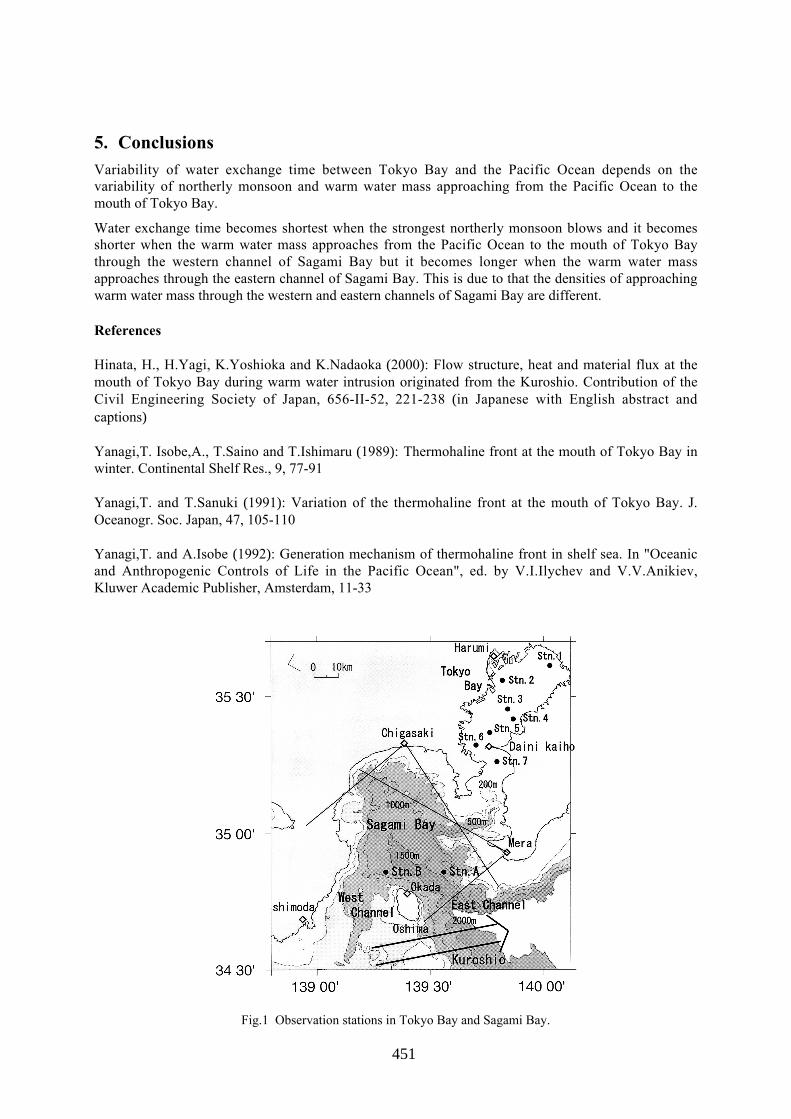
451

5. ConclusionsVariability of water exchange time between Tokyo Bay and the Pacific Ocean depends on thevariability of northerly monsoon and warm water mass approaching from the Pacific Ocean to themouth of Tokyo Bay.

Water exchange time becomes shortest when the strongest northerly monsoon blows and it becomesshorter when the warm water mass approaches from the Pacific Ocean to the mouth of Tokyo Baythrough the western channel of Sagami Bay but it becomes longer when the warm water massapproaches through the eastern channel of Sagami Bay. This is due to that the densities of approachingwarm water mass through the western and eastern channels of Sagami Bay are different.

References

Hinata, H., H.Yagi, K.Yoshioka and K.Nadaoka (2000): Flow structure, heat and material flux at themouth of Tokyo Bay during warm water intrusion originated from the Kuroshio. Contribution of theCivil Engineering Society of Japan, 656-II-52, 221-238 (in Japanese with English abstract andcaptions)

Yanagi,T. Isobe,A., T.Saino and T.Ishimaru (1989): Thermohaline front at the mouth of Tokyo Bay inwinter. Continental Shelf Res., 9, 77-91

Yanagi,T. and T.Sanuki (1991): Variation of the thermohaline front at the mouth of Tokyo Bay. J.Oceanogr. Soc. Japan, 47, 105-110

Yanagi,T. and A.Isobe (1992): Generation mechanism of thermohaline front in shelf sea. In "Oceanicand Anthropogenic Controls of Life in the Pacific Ocean", ed. by V.I.Ilychev and V.V.Anikiev,Kluwer Academic Publisher, Amsterdam, 11-33

Fig.1 Observation stations in Tokyo Bay and Sagami Bay.

452

Fig.2 Temporal variations in daily mean northward wind velocity at Daini-Kaiho and northward residual currentvelocity in the lower layer at Stn.6.

453

Sand Transport around a Coastal Headland: Portland Bill,Southern UK.ALEX BASTOS

(School of Ocean and Earth Science, Univ. of Southampton, Southampton OceanographyCentre, SO14 3ZH, Southampton, UK, [email protected])

MICHAEL COLLINS

(School of Ocean and Earth Science, Univ. of Southampton, Southampton OceanographyCentre, SO14 3ZH, Southampton, UK, [email protected])

1. IntroductionThe interaction between coastal headlands and oscillating rectilinear tidal currents results in theformation of tidal eddies (Pingree, 1978; Wolanski et al., 1984; Signell and Geyer, 1991). Thesignificance of coastal headland-eddies on the associated sedimentary processes has been pointed outby different authors, in terms of sandbank formation and/or facies and bedform distribution aroundheadlands (Pingree, 1978; Ferentinos and Collins, 1980; Signell and Harris, 2000; and Bastos et al., inpress). However, the effects of transient eddies on the instantaneous patterns of sediment transport stillrequire investigation.

Using a numerical simulation of the real environment, this investigation examines sand transportprocesses around a coastal headland (Isle of Portland, Southern UK, Fig.1). Likewise, the response ofthese processes in relation to the formation and evolution of tidal eddies. The inner shelf area underinvestigation is subject to semi-diurnal tides, with amplitudes of 2.4 m at Portland during spring tides.Overall over the region, the tidal currents tend to increase offshore and towards Portland Bill.Maximum spring current speeds, near the water surface, reaches up to 3.60 m s-1, at the tip of PortlandBill.

The principal objective is to study the potential patterns of sand movement (as bedload) and seabedmobility during the development of headland-associated eddies. Further, to examine how comparableare the final results of net (bedload) sand transport, with the tidally-induced residual circulation, interms of sandbank formation and sedimentary facies distribution.

2. MethodsThe study was undertaken using a 2-D finite element hydrodynamic model (TELEMAC, provided byHRWallingford (Hervouet, 1991)) combined with a sediment transport model (SEDTRANS, providedby the Geological Survey of Canada (Li and Amos, 1995)). Results from TELEMAC were provided,to the authors, by HR Wallingford in the form of original TELEMAC output files. These filescorrespond to two tidal cycles (25 hours) during spring and neap tides. The results are referred to thetidal signature only, with no consideration given to wind-driven currents.

SEDTRANS is an ANSI standard FORTRAN-77 numerical model. The model calculates bottom shearstress (for currents alone or under combined (wave and current) flows) and sediment transport rates,for input data of depth, current, wave, bed roughness and grain size. For the present study, thesimulations were carried out assuming a uniform grain size distribution over the inner shelf, due to thecomplex patterns of sediment distribution (including coarse lag deposits and bedrock outcrops (Bastoset al., in press). Three types of seabed were investigated: a coarse sand bed (D50 = 1 mm); a mediumsand bed (D50 = 0.5 mm); and a fine sand bed (D50 = 0.25 mm).

Threshold of sediment movement were calculated using SEDTRANS and compared with resultsobtained by flume experiments. The potential for bedload transport is investigated every 15 minutes(time-step).

454

Depth-averaged current data were input from the results obtained from TELEMAC. Bed shear stressand sediment transport rates were calculated by SEDTRANS, at each point of the original grid(triangular element mesh) imported from TELEMAC. Near-bed currents (1m above the seabed) werecalculated using SEDTRANS, by assuming a logarithmic velocity profile law. The bed shear stressunder currents alone was calculated by applying a quadratic friction law, using a friction factor(fc=0.006) based upon the field experiments of Sternberg (1972).

21005.0 ufcb ρτ =

Where, τb is the bed shear stress, ρ water density and u100 is the current speed 1 m above the seabed.Potential bedload transport rates were predicted/calculated, using the algorithm proposed by Gadd etal. (1978), for currents alone.

( )3100 cr

ss uuq −

= ρβ

Where qs is the bedload transport rate, β is an empirical coefficient (1.73 x 10-3), ρs is sedimentdensity, and ucr is the critical velocity for the initiation of bedload transport.

Figure 1: Area under investigation, showing main bathymetric features (Note: bathymetry in meters, relative toChart Datum).

3. Sand TransportBy simulating the potential bedload sand transport around a coastal headland, the non-linear nature ofsediment transport is taken into consideration i.e. instead of assuming that residual water circulationrepresents patterns of sediment transport. Because sand transport rates are calculated here based uponthe excess shear stress (where a critical threshold value must be reached before sediment initiatesmovement), instantaneous sand transport patterns do not necessarily follows the same transient patternas that of the tidal flow. Herein, this concept is observed clearly during the formation and evolution of

0 1 2 3 4 5

WeymouthChesil Beach

Isle

of

Port

land

(km)

Portland Bill

o

50 30’

o2 20’o2 35’

o

50 35’

Adamant Shoal

ShamblesBank

PortlandBank

West Shoal

PortlandDeep

455

tidally-induced transient eddies. Analysis of the hourly time steps during the tidal cycle, has revealedthat during the formation of the tidally-induced transient eddies, no current-induced bedload eddy isformed for either of the sand beds. The simulation of instantaneous sand transport over the tidal cyclehas shown that most of the bedload transport process occurs during the period of maximum flood andebb flows. At such times, gradients in bed shear stress and transport rates are also at maximum.

The significance of this pattern, to the understanding of sand dispersal around the headland, reliesupon the fact that these instantaneous gradients in transport rates occur upstream and downstream ofthe headland during the same part of the tidal cycle. Nevertheless, considering that currents, shearstress and bedload transport rates are at maximum at the tip of the headland, over the entire tidal cycle,a reverse in the transport rate gradient is observed as the flow passes the headland.

Thus, net sediment transport around a coastal headland represents instantaneous gradients in bedloadtransport rates, during flood and ebb flows, rather than the average flow. These gradients in transportrates lead to the formation of two distinct sand-mobile zones:

a) The inner sand transport zone. This zone is characterised by resultant sand transport towards thetip of the headland i.e. southward on both sides of the headland, followed by a downstream increase inthe transport rate gradient. Ebb and flood currents are constrained by the coastal geometry; they flowparallel to the coastline, then veer towards the south (with increased velocities), to follow the headlandcoastline. This zone is associated with the sand transport enhanced by the maximum ebb and floodcurrents; these flow parallel to coastline on the eastern and western sides, respectively.

b) The outer sand transport zone. This zone is situated offshore from the tip of the headland; it isdefined by sand transport away from the headland, with a downstream decrease in the transport rategradient. At the tip of the headland, the currents reach their maximum speed and a bottom frictionaltorque is induced, producing vorticity. When the flow leaves the tip of the headland, vorticity isadvected away into the flow, which starts veering towards the north. Because of these increasedspeeds at the tip of the headland, the currents leaving the headland are very strong and bedloadtransport rates are high. This process forms the outer sand transport zone, which is characterised by aveering in the sand transport vectors towards the north.

The boundary between the inner and outer zones defines a zone of bedload convergence.Consequently, this zone can be recognised on both sides of the headland, coinciding with the presenceof sandbanks (the Shambles and Portland Banks, Fig. 1). At the tip of the headland, a zone ofmaximum erosion occurs.

Furthermore, the occurrence of a suite of bedforms and sedimentary facies, described elsewhere(Bastos et al., in press) reinforce the results obtained here i.e. that the residual circulation is notappropriate to be used as a net sediment transport indicator. The sand transport pathways, indicated bythe asymmetry of large and very large sandwaves, corroborates the prediction of net bedload transport,as well as the occurrence of sandbanks associated with the bedload convergent zones.

4. ConclusionsThe instantaneous bedload sand transport patterns do not necessarily follow the same transient patternas that of the tidal flow; this is because sand transport rates are derived here on the basis of the excessshear stress, i.e. a critical threshold value must be reached, before the initiation of sediment movement.The numerical simulation has revealed that, during the formation of the tidally-induced transienteddies, no current-induced bedload eddy is formed for either of the sand beds.

Local characteristics and irregularities, in coastal and seabed morphology around the headland shouldbe considered as a parameter for modelling tidal and sand dispersal around headlands. Despite thesame magnitude of different length-scale parameters (such as tidal excursion, headland dimensionsand bottom friction), net sand transport rates do not follow the pattern of residual (water) circulation

456

over the study area. Neither could the concept of sandbanks occurring in the centre of residual eddiesbe verified.

Sediment transport and erosion around coastal headlands is defined by the presence of a zone ofmaximum erosion at the tip of the headland (maximum transport rates) and by occurrence of twodistinct zones of sand transport: (a) an inner zone showing sand transport towards the headland,following an increase gradient in the sand transport rates; and (b) an outer zone showing sand transportaway from the headland, following a decrease in the transport rate gradient.

Acknowledgments: During the research, the first author (ACB) was supported by a Scholarship awarded by theConselho Nacional de Pesquisa (CNPq, Brazil). The authors would like to acknowledge: HR Wallingford andWessex Water Authority, for providing the output data from TELEMAC; and the Geological Survey of Canada,for providing the SEDTRANS92 model.

References:

Bastos, A.C., Kenyon, N.H. and Collins, M.B., Sedimentary processes, bedforms and facies,associated with a coastal headland: Portland Bill, Southern UK. Marine Geology, in press

Ferentinos, G. and Collins, M. B.,. Effects of shoreline irregularities on a rectilinear tidal current andtheir significance in sedimentation processes. Journal of Sedimentary Petrology, 50(4), 1081-1094,1980

Gadd, P. E., Lavelle, J. W., and Swift, D. J., Estimate of sand transport on the New York shelf usingnear-bottom current meter observations. Journal of Sedimentary Petrology, 48, 239-252, 1978.

Hervouet, J. M., TELEMAC, a fully vectorised finite element software for shallow water equations.HE43/91-27, Electricite de France, 1991.

Li, M. Z. and Amos, C. L., SEDTRANS92: A sediment transport model for continental shelves.Computers & Geosciences, 21(4), 533-554, 1995.

Pingree, R. D., The formation of the Shambles and other banks by tidal stirring of the seas. Journal ofthe Marine Biological Association U K, 58, 211-226, 1978.

Signell, R. P. and Geyer, W. R., Transient eddy formation around headlands. Journal of GeophysicalResearch, 96(C6), 2561-2575, 1991.

Signell, R. P. and Harris C. K., Modeling sandbank formation around tidal headlands. In Proceedings6th International Conference Estuarine and Coastal Modelling, edited by Spaulding, M.L. andBlumberg, A.F., New Orleans, LA, November 1999. ASCE Press, 2000.

Sternberg, R. W., Predicting initial motion and bedload transport of sediment particles in the shallowmarine environment: In Shelf sediment transport, processes and pattern, edited by Swift, D. J., Duane,D. B., and Pilkey, O. H., Dowden, Hutchison and Ross, Inc., Stroudsburg, Pennsylvania. pp61-83,1972.

Wolanski, E., Imberger, J., and Heron, M., Island wakes in shallow coastal waters. Journal ofGeophysical Research, 89, 10553-10569, 1984.

��

�� !"� #$ �% ��

�� &��'�� &�� ( " �))�� *� " � ��

� ��

�� !� �� "�� #��$�� $�� %�� &�� #��$�� !�� $�� '()*+, �� -�� !�� .�� /.�� 0�� (� �� 1� �� /�� 0�� (� �� 1� �� .��

� � ��

�� .�� %�� 2�� &�� &�� $�� $�� /34 �1 ��$�� %�0�� ( �� .�� /0�� 3� �� 1 ��"� �� 5 /(1 �� .�� /31 � �� /61��

0�� (5 �� 5 7�� %� �� .�� ())( /�� 1�())8 /�� 1� �� ())+ /�� 1�

� ��

�� -�� %�� 9�� .�� 9�� :�� :�� 9�� %�� ;0�6� �� /�� '())8,1�� ;0�6�$0; : �� #�� %� � �� $�� 9��!� �� -�� .�� $�� -�� 7�� 2��<��!�� /7�2<1 �� '�� ())),� �� /��&3� &8� &*� 931 ��

0�� 35 ;�� <��5 �� /��1 �� /��1 �� ())($())+� &�� <��5 2�� /��1 �� /��1 �� &4$&3 �� =�� <��5 9�� &3$&8 �� .>� ��

�� '3443,�

� ��

�� .�� -�� $ /�� 1 �� $�� -�� $�� %� �� ?�� /�� '3444,1 �� '()*+,� %� ��

� @�� A � B �� 4� /(1

�� B �� #�� /&31 �� B� �� !�� 7 �� '())+,�� $�� ( �� 0�� B 4� �� -�� %� �� $�� 7�� /&41� �� &3�� &8 �� -�� %� �� /&4$&3 ��&3$&81 ��

! "��

0�� 3� �� /�� $�� &4$&3 ��1� �� .�� 0�� /�� &3$&8 ��$�� 1 �� 2�� #�� 0�� /��1 �� ?��

"��#

>�� C�D�� 2�� <��$ �� &�� :�� &�$�� 9�� %�� !""!# ��$� 3443 /�� 1�

D�� <�� %� &� �� '� E*8F*+8� ()*+�

=�� G�� ?�� 7 �� .�� 9�� %�� !(� 8(F8H� ())+�

=�� G�� I�� G�� G�� 0�� G�� 0�� &�� .�� 9�� :�� 9�� )�*�**& �� +,,,# �� ()))�

=�� C� 7� �� D� J� 0� &� �� >�� ;0�6�� -.�� +,,/� >�� =��$�� 8E(F8EE�())8�

I�� J�� C� �� :� �� 0�� 0�� # �� &�� K�� 9��!� <�� 2�� (6)F(E)� 3444�

461

Buoyancy Driven Current during Cooling Periods in IseBay, JapanTATEKI FUJIWARA

(Graduate School of Agriculture, Kyoto University, Kyoto, Japan, [email protected])

1. IntroductionThe process of convection in rotating fluids has been intensively studied over the last decade. It hasbeen revealed that the convection phenomenon is sensitive to spatial inhomogeneities in the coolingintensity and to the preexisting stratification. As a result, lateral gradients in density and mixed-layerdepth are formed. These lateral density gradients drive a thermal-wind circulation. The shear of thethermal-wind modifies upright convection to slantwise convection; the overturning fluid movessystematically in slanting paths and maintains a nonvanishing stratification [Haine and Marshall,1998; Review by Marshall and Schot, 1999].

Spatial inhomogeneities in buoyancy flux and stratification are typical aspects of water in regions offreshwater influence (ROFI). Buoyancy is supplied laterally from the river mouth as freshwaterdischarge and lost upward through the sea surface as heat. In general, the stratification is stronger nearthe river mouth than in the offshore area due to salinity stratification. Therefore, it is expected thatcooling exerts an influence on both freshwater spreading and basin-wide estuarine circulation inROFIs.

In this work, we have studied a buoyancy driven current and resultant basin-wide estuarine circulationin Ise Bay, Japan during a cooling period. We have made use of the following working hypothesis:that surface cooling causes convection and mixed-layer deepening in the bay whereas the mixed-layerremains shallow in the region where river plume caps the surface; this difference in the mixed-layerdepth creates a horizontal density gradient, which drives rotation of the deep mixed-water mass inthermal-wind balance. To verify this hypothesis, we conducted a series of longitudinal hydrographicobservations from the bay head (river mouth) to off the bay mouth at roughly 10-day intervals over aperiod of 1.2 years. Prior to these observations, we simultaneously measured flow structures anddensity fields by using ADCP and CTD techniques during a cooling period in 1994 [Fujiwara et al.,1997]. Flow fields were calculated from the measured density field by using a diagnostic numericalmodel and compared with the flow fields measured with the ADCPs. This data set was also used tospecify the flow structure in the cooling period. In this paper, hydrographic properties and flowstructures during cooling period are described and above working hypothesis is verified.

2. Results and discussionLongitudinal distributions of salinity and temperature measured on 27 October 2000, 26 January 2001and 13 February 2001 are presented in Figure 1. These dates fall in the early, central, and late stages ofthe cooling period, respectively. Density distributions (not shown) are similar to the salinitydistributions for all dates. Towards the end of October (Figure 1a), hydrographic conditions in the Bayhave changed from a strongly stratified to a weakly stratified regime. A well-defined halocline (31 < S< 32) separates the upper water from the lower water. The river plume, which is characterized by lowsalinity (S < 30), covers the bay head area from the river mouth to station 3, while well-mixed water,which has salinity 30 ~ 31, occupies the upper 20 m between stations 3 and 5. Hereinafter, we refer tothe former and latter areas as the river plume region and the convection region, respectively.

The halocline is shallow in the river plume region (depth ~ 10 m) and deep in the convection region(depth ~ 20 m). The mixed-water mass exhibits a reversed-dome shape in the convection region. Werefer to this water mass as a mixed-water lens. Considering the rotational effect, we can expect thatthis mixed-water lens is rotating anti-cyclonically.

462

(a)

(b)

(c)

Bay Head Irago Strait1 2 3 4 5 6

0

20

40

De

pth

(m)

0

20

40

Dep

th(m

)

0

20

40

Dep

th(m

)1 2 3 4 5 6

0 20 40 60

Distance (km)

0 20 40 60

Distance (km)

L31

32

32.632.6

HL

H

L

H

1010

9

H

L31 32

33H

33

33.4

H

L29

30

313233

H

L21

H

H22

L21.6

9.410 11

12

H

H

Figure 1 Longitudinal distributions of salinity (left) and temperature (right) observed on 27 October 2000 (a), 26January 2001 (b), and 13 February 2001 (c). The abscissa is distance from the bay head measured along the

thalweg.

The features described above are common to hydrographic conditions measured on other dates.However, the mixed-water mass expands and almost reaches the bottom on 26 January (Figure 1b).The river plume region shrinks in a narrow range near the river mouth, due to the decrease in riverdischarge. In this region the water is still strongly stratified.

Horizontal distributions of salinity at the surface and at 15 m depth in the late October are representedin Figures 2a and 2b, respectively. The river plume water covers the northern half of the bay (Figure2a), while homogeneous mixed water (31 < S < 32) extends to the southwest of the river plume front(S = 31). In contrast to the surface salinity distribution, the salinity at 15 m depth is lower in the souththan in the north (Figure 2b). This somewhat peculiar phenomenon is caused by the fact that thehalocline is shallower than 15 m in the north and deeper than 15 m in the south. The shaded area,where S < 32, represents the area of the convection region. This region is surrounded by a band ofcrowded isohalines along its northeastern periphery.

Horizontal distributions of the residual flows at the surface calculated by the diagnostic model aredepicted in Figures 2c, together with the trajectories of water particles tracked for 6 days (Figure 2d).The surface flow pattern is highly correlated with the salinity distribution at deeper level (Figure 2b).The water in the convection region rotates anti-cyclonically. The water strongly flows along a coursetraced by the band of crowded isohalines at 15 m depth, which surround the convection region.

463

An anti-cyclonic circulation occupies the convection region. Due to this circulation, strong southwardflow (jet) arises along the east coast. On the other hand, western water in the bay slowly flows to thebay head along the southwestern coast. This direction opposes the direction of the basin-wideestuarine circulation in the upper layer. Because strong flows concentrate in relatively narrow belts,water particles released off the river mouth are conveyed along the meandering pathways on theirjourney to the sea (Figure 2d).

137ßE40'

35ß

137ßE

40'

40'

(c) (d)

10 cm s-1N

137ßE40'

35ß

137ßE

40'

40'

(a) (b)

H

H L

32

33

H

H

H

32

31

30

28

22L

LL

N

Figure 2 (a) Salinity distribution at the surface, (b) that at 15 m depth measured on 29 and 30 October 1994, (c)flow field at the surface calculated by the diagnostic model, and (d) trajectories of water particles tracked for 6

days.

464

Convection

(Anticyclonic

(Buoyancy loss)(Buoyancy supply)Freshwater inflow

L. salinity

Isolated water circulation)

Cooling

H. salinity

Well-mixed water

Figure 3 Schematic illustration of hydrodynamic condition and buoyancy driven currents during coolingperiods.

The results obtained in this study are schematically illustrated in Figure 3. In the river plume region,strong salinity stratification stabilizes the water column and suppresses convective mixing. Here thepycnocline is shallow, whereas it is deep in the convection region. In the central bay, the deepening ofthe mixed water generates a light-water lens, which rotates anti-cyclonically under the geostrophicbalance. The location of the lens varies depending on the river discharge. In addition, theaccompanying anti-cyclonic circulation also changes its location. When the river discharge decreases,the lens approaches the river mouth. The location and size of the circulation exert large influences onthe basin-wide flow fields.

Acknowledgments. The auther thanks Y. Sugiyama of Chyubu Electric Power Co., Inc., who conducted theobservations in 1994, and also T. Kimura and the crew of R/V Iseshio of the Japan Coast Guard, whoaccomplished the longitudinal observations in 2000 ~ 2001 with A. Kasai of Kyoto University. The auther alsothanks Dr. J. P. Matthews for improving this manuscript and appreciates the help of M. Fujihara of EhimeUniversity and S. Kakehi of Kyoto University in the numerical model analysis.

References:

Fujiwara, T., Sanford, L.P., Nakatsuji, K., and Sugiyama, Y., Anti-cyclonic circulation driven by theestuarine circulation in a gulf type ROFI, J. Marine Systems, 12, 83 - 99, 1997.

Haine, T. W. N. and J. Marshall, Gravitational, symmetric, and baroclinic instability of the oceanmixed layer, J. Physical Oceanography, 28, 634 - 658, 1998.

Marshall, J. and F. Schott, Open-ocean convection: observations, theory, and models, Reviews ofGeophysics, 37, 1 - 64, 1999.

465

Role of straits in transport processes in the Seto InlandSeas, JapanXINYU GUO

(Center for Marine Environmental Studies, Ehime University, 3 Bunkyo, Matsuyama 790-8577, Japan, [email protected])

AKIRA FUTAMURA

(Graduate School of Science and Engineering, Ehime University, 3 Bunkyo, Matsuyama 790-8577, Japan, [email protected])

HIDETAKA TAKEOKA

(Center for Marine Environmental Studies, Ehime University, 3 Bunkyo, Matsuyama 790-8577, Japan, [email protected])

1. IntroductionAs one of the most important coastal water,the material transport processes in the SetoInland Sea are always an important issue inthe Japanese coastal oceanographycommunity (see Takeoka [2002] for areview). With the community to attach moreand more importance to the role of thenutrient from the open ocean, the processesto distribute the nutrient in the sea must alsobe paid attention.

One important feature of the Seto Inland Seais that there are as many as about 1000islands in the sea. No matter of the size ofislands, they form many straits andrelatively extensive sea regions (Nada inJapanese). Forced by the tide wave from thePacific, the ability of tide mixing is thereforecompletely different between the strait andNada. As expected, tidal front is formed inmany places in the Sea (Yanagi[1990]).Although the geostrophic componentprevents the cross front material transport,the ageostrophic component is suggested topromote the exchange of nutrient betweenthe upper and bottom layer in the stratifiedregion with a path through the mixing region(Takeoka[2002]).

In this study, we choose Hiuchi Nada (Fig.1)as a representation of such strait-Nadasystem. Hiuchi Nada is located in the central part of the Seto Inland Sea. Its size is approximately50km_30km and its average depth is 20m. Except for the Bisan Seto, the river discharge into thisNada is small. Its western and eastern boundaries are the Kurushima Strait and Bisan Seto,respectively (Seto means region of strong current in Japanese). The tide in the Hiuchi Nada ischaracterised as a standing wave and the M2 tidal amplitude is about 1m. Along with the sea levelchange in the Nada, the tidal currents at the Kurushima Strait and Bisan Seto are naturally very strong

Figure1: Map of Seto Inland Sea (upper panel) andHiuchi Nada (lower panel)

466

and the water there is well mixed throughout a year. On the other hand, as a result of the weak tidalcurrent, the heating in summer usually induces a strong stratification in the eastern part of the Nadawhere the oxygen-deficient water mass is usually found in the bottom layer.

Up to now, because of the social impact of the oxygen-deficient water mass, the studies in the HiuchiNada were almost concentrated on its eastern region. Here we treat the Hiuchi Nada, Kurushima Straitand Bisan Seto as a whole system. With repeated CTD observations over the whole Nada and the useof a numerical model, we want to clarify the distribution of water masses, their formation processesand the related residual current field.

2. Observations and resultsSeven times of ordinary CTD observations were carried out in the summers of 2000 and 2001. Figure2 shows the distribution of CTD stations and Table 1 the dates of each observation and observedstations. The measurements were always finished in one day.

Figure 3 shows the distribution of water temperature at three layers. In the upper layer (2m depth), anobvious warm core exists in eastern region while the western region is low temperature; in the middlelayer (10m depth), the central part shows a high temperature while the western and eastern sidesshows a little of low temperature; in the lower layer (20m depth), a clear cold core is found in theeastern area. In the northern area, partially mixed warm water exists, which might come from theshallow Bisan Seto.

1

2

34

5

67

8

91 0

1 1

1 21 3

1 4

1 51 6

1 7

1 8

ABC

DE

F

G

HI

J

Figure2: Distribution of CTD stations

In general, the vertical difference of temperature increases from Kurushima Strait to the eastern part ofHiuchi Nada. And, the horizontal temperature gradient is relatively weak in the middle layer butstrong in the upper and lower layers.

Date Station

2000 Aug. 1-2 1,2,3,4,5,6,7,8,9,10,11,12,13,14,15,16,17,A,B,C,D,E,F,G,H,I

2000 Aug. 28 1,2,3,4,5,6,7,8,9,10,11,12,B,C,F,G,H

2001 May. 27 4,5,6,8,11,14,17,C,D,E,G,J

2001 Jul. 1 2,3,4,5,8,9,10,11,14,15,16,17,B,C,D,E,F,G,J

2001 Jul. 25 4,5,8,9,10,11,14,15,16,17,C,E,F,G,H,I

2001 Aug. 8 1,2,3,4,5,6,7,8,9,10,11,12,13,14,15,16,17,18,A,B,C,D,E,F,G,H,I,J

2001 Sep. 25 1,2,3,4,5,6,7,8,9,10,11,12,13,14,15,A,B,C,D,E,F,G,H,I,J

Table1: Stations and dates of observations.

467

24. 5

25

2525. 5

27

26

26

25. 5

2525.5

26

(a). Depth=2m

25

25

24. 5

24. 5

23

23. 5

24.5

24. 5

23

(b). Depth=10m

21. 5

22

22.5

22. 5

23

23

24

24

24. 5

23

(c). Depth=20m

Figure 3: Horizontal distribution of water temperatureat the depth of (a)2m, (b)10m, (c)20m in Hiuchi Nadaon Aug.1 2000

3. Numerical model and resultsBased on Princeton Ocean Model (POM), a numerical model for the Hiuchi Nada, Kurushima Straitand Bisan Seto is configured. The horizontal resolution is about 500m and there are 20 layers in thevertical. The model are driven by the tidal current, heat fluxes, river discharge, wind stresses and theflow-in or flow-out residual current along its western and eastern boundaries. The necessary harmonicconstants of tidal current along the western and eastern boundaries are calculated by a tide model forthe whole Seto Inland Sea.

The model results are saved every hour and a digital filter (Hanawa and Mitsutera[1985]) is used toremove the tidal signal. In addition to the ordinary diagnostic and prognostic calculation for residualcurrent, several tracer experiments are also carried out in order to clarify the fate of passive materialinitially set in the Straits and Nada.

Here we only show the variation of sea level and M2 tidal current during 12 hours (Fig.4) thatdemonstrates a clear standing wave characteristic. As the sea level reaches its positive or negativemaximum value at 1 or 7 h, the tidal current in the Kurushima Strait is weakest; as the sea levelbecomes almost flat at 4 or 10 hour, the tidal current in the Kurushima Strait is strongest. Moreover,the strength of tidal current varies largely horizontally, that is, in the eastern part of Hiuchi Nada thetidal current is always as weak as 10~20cm/s while those in the Kurushima Strait and Bisan Seto couldbe over 1~2 m/s.

Taking this tidal field as the background, we carried out some numerical experiments to clarify theinfluence of heating, river discharge, wind and forcing at lateral boundaries on the residual currentfield and the formation of stratification. The results as well as those of tracer experiments will bepresented in the presentation.

468

Figure 4: Variations of sea level and M2 tidal current in the Hiuchi Nada during 12 hours.

Acknowledgments: This research is supported by Grant-in-Aid for Scientific Research (A) from Japan Societyfor Promotion of Science (No. 12308027).

References:

Takeoka, H., Progress in Seto Inland Sea Research, Journal of Oceanography, 58, 93-107, 2002.

Yanagi, T., Temporal and spatial variations of coastal fronts in the Seto Inland Sea, Japan, in Physicsof Shallow Seas, ed. Wang, H-T., et al., China Ocean Press, Beijing, 279-290, 1990.

469

Effects of steep topography on the flow and stratificationnear Palmyra AtollILSE M. HAMANN

(Institute of Oceanography, University of Hamburg, Troplowitzstrasse 7, 22529 Hamburg,Germany, [email protected])

GEORGE W. BOEHLERT

(Oregon State University, Hatfield Marine Science Center, 2030 SE Marine Science Dr.,Newport, OR 97365-5296, USA, [email protected])

CHRISTOPHER D. WILSON

(NMFS Alaska Fisheries Science Center, RACE Division, 7600 Sand Point Way NE, Building4, Seattle, WA 98115-0070, USA, [email protected])

1. Introduction

Two interdisciplinary cruises aimed at relating the ecology of marine fish populations tooceanographic conditions were fielded during the late summer and late winter seasons (1990 and1992) near Palmyra Atoll (5.9 ºN, 162.1 ºW) in the Line Islands in tropical Central Pacific.

2. Background circulation and flow around Palmyra Island

During the first cruise (August/September 1990) satellite-tracked surface drifters and acoustic Dopplercurrent profiler (ADCP) measurements showed a strong eastward setting North Equatorial CounterCurrent (NECC), with maximum speeds exceeding 1 m sec -1 at about 80 m depth (Fig. 1). Thiscurrent turned southeastward on closer approach to Palmyra.

Figure 1: Vertical profile of eastward and northwardADCP current components in the core of the NorthEquatorial Countercurrent at 163 °W longitude. Data areaveraged over 10 m depth intervals. Data from TC90-07(solid lines) is at 6°N latitude; TC92-01 (dashed lines) is at5.6°N latitude.

The drifter paths exhibited excursions with zonal wavelength of about 250 km, meridional amplitudeof 25 km, and period of about 5 days. These undulations can be explained as expressions of inertialwaves in the presence of a northward pressure gradient, and are excited by windbursts or suddenweakening of the steady northeast trades. A detail of the path of one drifter during one inertial periodafter a total slackening of the winds is shown in Fig. 2.

470

Figure 2: Path of drifter 15087 (TC90-07) nearPalmyra demonstrating inertial oscillation.

During the second cruise (February/March 1992), the ADCP-derived speeds of the NECC wereweaker (maxima about 33 cm sec -1) while the relative geostrophic flow component was of similarmagnitude to that in 1990 and the signal of zonal geostrophic currents reached much deeper to about650 m depth as compared to 150 m in 1990.

In the relatively thick upper mixed layer (75 to 100 m) the eastward flow decelerated on approach ofthe island in 1990 between 163 ºW and 162.2 ºW, but increased again off Palmyra�s north and southflanks (Fig. 3). Close to Palmyra�s north and south shores there was a zone of retardation of thealongshore currents and weak offshore components. In fact, this area of reduced flow extends out tothe eastern downstream waters in the lee of the island, where an area of flow reversal occurs (u < 0 cms-1 ). In this vicinity the contours of the corresponding meridional current component v exhibit a richstructure as well, indicative of some island wake pattern, for example an attached and one or twodetached eddies off Palmyra�s southeast corner.

Figure 3: Contours of layer-averaged ADCP eastward (u) and northward (v) current velocity components aroundPalmyra Atoll, core of the NECC (55-111 m, TC90-07).

The observed convoluted flow structure off Palmyra led us to investigate criteria for flow separationthat were derived theoretically and/or from laboratory experiments. We estimated parameters ofturbulent 2-dimensional wake theory, e.g. Rossby, Ekman and Reynolds numbers from thetopographic dimensions, flow speeds, Coriolis acceleration, and a range of values for the turbulenteddy viscosity. While the resulting numbers are suggestive of formation of eddies in the lee of theisland, we did not, however, detect any circular motions with the sampling and instrumentationapplied during either expedition.

3. Thermohaline structure at Palmyra Atoll

Doming isopycnals beneath the surface mixed layer as well as thick (20-40 m) internal mixed layerswere found near Palmyra during both cruises, with slightly different position relative to the island

471

(Fig. 4). The discontinuous vertical temperature profiles may have been a result of strong boundarymixing due to breaking internal waves on Palmyra�s steep slopes (Fig. 5).

Figure 4: Depth profiles of temperatureand density at two CTD stationsa) during TC90-07: CTD Stn. 6, dottedline; CTD Stn. 35, solid line.b) during TC92-01: CTD Stn. 6, dottedline; CTD Stn. 58, solid line.

Figure 5: Spatial distribution of the intensity of vertical mixing between 100 and 300 m. Contours are thevariance of the vertical temperature gradient dT/dz (x 104) taken over 2 m vertical distances between the 100 and300 m depth horizons. a) TC90-07; b) TC92-01.

In the immediate vicinity of the island variations in flow speed, stratification and �mixing� both in thealongshore and cross-isobath directions were observed.

4. Conclusions

Ocean current and hydrographic measurements made in two different seasons and two years apart nearan island located in the eastward setting North Equatorial Counter Current revealed interaction of theflow with the steep topography on large, intermediate and small spatial scales.

Overall, the current speeds were reduced during the second cruise in February/March 1992, the peaktime of the 1991-1993 warm event in the tropical Pacific.

Paths of drifters drogued in the surface layer during the first cruise in August/September 1990 suggestthat a combination of atmospheric and topographic forcing may have been responsible for theobserved veering of the drifters east of the island.

The location with its observed high energy motions appears to be suitable for another experiment withstate-of-the-art turbulence instrumentation and derivation of more accurate estimates of the turbulenteddy viscosity, turbulent energy dissipation rates and mixing, all of which are crucial quantitives foran accurate description of near-island marine ecosystems.

472

Resuspension process of muddy sediments in Tokyo Bay,JapanYASUYUKI NAKAGAWA

(Port and Airport Research Institute, Nagase 3-1-1, Yokosuka 239-0826, Japan,[email protected])

1. IntroductionSince fine sediment particles such as silt and clay are easily stuck with contaminants, it is importantsubject to study fine sediment transport processes in estuarine and coastal area for restoration andmaintenance of their environment. The transportation and deposition rate of fine sediments depends ondifferent external force conditions and supply processes of sediment etc. In case of less tidallydominated and shallow estuary, wind waves have a key role of sediment transport processes (Sanford1994). In order to examine the mobility of muddy bottom sediment by waves, a field observation wascarried out at inner Tokyo Bay (Fig.1), where tidal energy is not so strong and wave is considered tobe a key factor for sediment transport process.

2. Field ObservationsThe resuspension studies were carried out over 15 days during February in 2001 at the site in TokyoBay as shown in Fig.1. The site is 3km off the north east coast of the bay with average depth of about10m. In order to see time variation of suspended sediment concentration near the bottom, opticalbackscatter sensor was set so that the measuring point is 10cm above the bottom. Out put of the OBSwere subsequently converted to total suspended particulate concentration in mg/l by applying acalibration result with Kaolin clay. For measurement of particle size of suspended sediment, an in-situtype particle size analyser, LISST100 (Agrawal and Pottsmith, 2000), was also set next to the OBS.Turbidity and particle size distribution were recorded at 5 min and 30 min intervals respectively. Forcurrent measurement, an electro magnetical current meter was set to measure current velocity 50cmabove the bed. Pulse-coherent type acoustic Doppler velocity profiler was also used to get the verticalprofile of near bottom current with high resolution record in space and time, 5cm pitch vertically and2Hz for 2min burst every 30min. Ultrasonic type wave meter was set to measure the wave condition.Sediment traps were deployed 3 times during the survey period and cylinders (caliber: 15cm) were setwith trap level of 1m and 2.7m above the bed. Trapped matters are applied for analysis of wet and dryweight, particle size, and organic matter concentration.

Figure 1: Tokyo Bay and location of study site.

473

3. Results(1)Relationship between SS concentration and external forces

Time series data of wind, near bottom current (averaged in 10 min.), and wave during the period withrelatively higher wind condition is shown in Fig.2. The bottom shear stress induced by waves is alsoindicated in the figure, which was estimated as maximum bottom shear stress due to waves with thefollowing equation (e.g. Grant and Madsen 1986).

τb = 1/2 fW ρUb2 (1)

where ρ is the density of the water. Ub , the maximum orbital velocity near the bottom, was obtainedas the value of monoclomatic wave with significant wave hight and period through the linear wavethory. The wave friction factor, fw, was set as 0.03 considering a typical wave period and sedimentgrain size in the area.

The bottom current due to wind exceeds 10cm/s in the afternoon on February 16, 2001, which is thehighest record during the deployment, but apparent resuspension of the sediment does not occur underthe current. On the other hand, the suspended sediment concentration above the bed was extremelyincreased under the effect of the wave induced bed shear stress in the before noon on February 16,2001, and the result implicates that waves play a key role for sediment transport process in the bay.Although the wave height was still high in the afternoon of the day, waves less disturbed the bottomsediment because wave period became relatively short due to the change in the wind direction.

Figure 2: Temporal evolution from wind velocity vectors, bottom current speed, significant wave height,significant wave period, bed shear stress due to wave and suspended sediment concentration above the bedduring the observation.The events of resuspension of sediment due to wave occur twice during the observation.

474

In order to examine the critical shear stress for these resusupension or erosion of the bed by the effect of waves,suspended sediment concentrations are compared with the bed shear stress due to wind waves in Fig.3. Thesuspended sediment concentrations drastically increase between the shear stress of 0.001-0.01 Pa and it maycorrespond to the range of critical shear stress for erosion.

Figure 3: Relationship between suspended sediment concentration and bed shear stress due to waves.

(2)Particle size distribution characteristic of suspended sediment

Figure 4 shows the size distributions of suspended sediment in the volume concentration measuredwith LISST-100, comparing the data during high wave event and calm conditions before and after theevents on February 16 (Left fig.) and 22 (Right fig.), 2001. Both particle size distributions during theresuspension events measured at 6:00 on February 16, and at 1:30 on February 22 have a peak around200 µm with a second peak around 20-30 µm. The similarity of the particle size distributions betweenthese suspended sediment and bottom sediment shown in the Fig.5 indicates that the suspendedsediment during wave events are dominated by the bottom sediment at the study site rather thanadvected from surrounding area.

Figure 4: Particle size distribution of suspended sediment during resuspension events.

475

Figure 5: Grain size distribution at the study site (St.1).

4. ConclusionsField observation of turbidity, current and waves during the winter of 2001 in Tokyo Bay has revealedthe following aspects. (1) Wind waves are more dominant than tidal current for resuspension of thesediment at the study site. (2) Critical bottom shear stress induced by wind waves is estimated between0.001-0.01Pa, and (3) Particle diameter distribution of suspended particles near the bed during theperiod of wave forced resuspension event is close to the grain size distribution of the bottom sediment.

References:

Agrawal,Y.C., and H.C.Pottsmith (2000):Instruments for Particle Size and Settling VelocityObservations in Sediment Transport, Marine Geology,Vol.168,pp.89-114.

Sanford, L.P. (1994): Wave-Forced resuspension of upper Chesapeake Bay Muds, Estuaries, 17,No.1B, 148-165.

Grant, W. D., and O. S. Madsen (1986): The Continental-Shelf Bottom Boundary Layer, Ann. Rev.Fluid Mech. 18,pp.265-305.

476

Numerical modelling of suspended matter transportANDREI PLESKATCHEVSKI

(GKSS Research Centre Max-Planck-Str.1, D-21502 Geesthacht, Germany, [email protected])

GERHARD GAYER

(GKSS Research Centre Max-Planck-Str.1, D-21502 Geesthacht, Germany,[email protected])

WOLFGANG ROSENTHAL

(GKSS Research Centre Max-Planck-Str.1, D-21502 Geesthacht, Germany,[email protected])

1. IntroductionIn many satellite borne ocean colour images of the North Sea a plume is visible, which is caused bythe scattering of suspended particulate matter (SPM) in the upper ocean layer [Doerfer and Fischer1994] (cf. Fig.1). This structure can be seen in most ocean-colour images with different intensity andit is particularly visible after strong storm events. The origin of the plume is located near to the cliffsof Suffolk, Great Britain, and it extends along the coast of the Netherlands and Germany towardsDenmark. The intensity and length of the plume varies and depends strongly on the local current andwave field. The objective of this study is to investigate the cause of the development of the plume andto set-up a numerical model. SPM concentration is governing the light attenuation, which is importantfor primary production.

A Suspended Particulate Matter Transport model (SPMT), which can be operated in a quasi 3-D and afully 3-D mode, was developed for the North Sea. The fully 3-D model is presently implemented as aSPM module into the operational transport model of the Bundesanstalt für Seeschifffahrt undHydrographie (BSH). The module contains the following processes: settling of SPM, verticalexchange due to currents and waves in the water column, sedimentation, re-suspension and erosion inthe bottom layer, and processes of bioturbation and diffusion in the upper 20 cm of the bottom layer.The main new aspect of the model is the derivation of the vertical exchange considering the localcurrent speed and wave height. Calibration was done with satellite data of surface SPM concentration.

Figure 1: Model area and SPM retrieved from theSatellite Borne Coastal Zone Colour Scanner (SCZC)

477

2. Set-up of SPM modelsThe BSH transport model calculates the transport on nested grids with a horizontal resolution of 6 nmfor North and Baltic Sea and 1 nm for the German Bight with up to 9 vertical layers. The forcing oferosion und sedimentation processes results from the local shear stress velocity derived in time andspace under consideration of currents and waves according to Soulsby [Soulsby 1997]. In the modelthe sources of SPM are rivers, concentration at the open boundary, bottom sediment and erosion atthree English cliffs Suffolk, Norfolk and Holderness. 3 SPM fractions with different settling velocitiesare considered.

The vertical exchange coefficient Av is assumed to be the sum of the vertical exchange due to currentsAv

cur and due to waves Avwav:

A z A z A zv vcur

vwav( ) ( ) ( )= + , (1)

A z K U z Tvwav

wav wav( ) ( )= ⋅2 2 , (2)

A z Kdu

dzvcur

P( ) = 2 , (3)

Where z is the vertical coordinate, Uwav is the orbital velocity of the significant wave, T is the waveperiod and u is the current velocity. The coefficients Kwav - a function of significant wave height - andKP - the Prandtl mixing length (m) - are unknowns, which have to be determined in synergy withocean colour satellite data.

The computation of the SPM bottom processes considers bioturbation by benthos (crabs and worms)and diffusion in the upper 20 cm of the bottom layer.

The main new aspects of the model are dependency of cliff erosion on significant wave height andderivation of vertical exchange on consideration of local current speed and wave height using oceancolour data from MOS and SCZC satellites for calibration and validation.

From the yearly mean erosion rates [Puls et al 1997] of the Suffolk, Norfolk and Holderness cliffs andthe statistics of significant wave height Hs in the years 1993-1995 constant factors have been estimatedfor storms (Hs >2m) and calm weather (Hs <2m) to distribute the yearly erosion over significant waveheight.

3. Vertical exchange coefficientIt is assumed that the SPM plume structure at the surface results from the vertical SPM distributionmainly caused by vertical mixing processes due to currents and waves. This distribution can bedescribed with a profile function determined by SPM settling velocities and vertical mixing processes.The surface SPM concentration, known from satellite ocean colour images, is the upper boundarycondition of this profile. In synergy with the results of the two dimensional transport model,determining the mean concentration in the water column, the vertical exchange coefficient Av isadjusted.

In the quasi 3-D model the vertical distribution of SPM is given by:

C z C e

w z

Asur

s

v( ) = (4)

478

Where Csur is the surface SPM concentration, ws the settling velocity of SPM, Av the vertical exchangecoefficient, and z the vertical coordinate.

The vertical mean SPM concentration is defined as:

Ch

C z dzh

= ∫1

0( ) (5)

Replacing C(z) in (5) by (4) and solving the integral results in:

CC

h

A

wesur v

s

wsh

A v= ⋅ −

1 (6)

The surface SPM concentration from CZCS and MOS images acquired during calm weather and themean SPM concentration retrieved from the SPM transport model the current component Av

curof the

vertical exchange coefficient can be calculated. The storm periods [Hetscher et al. 1998] are used to

derive the wave component Avwav

.

In a second step the parameters Kp and Kwav for A zvcur ( )and A zv

wav ( ) of the fully 3-D model are fitted.

4. Erosion depth parameter and SPM bottom depositsFor most areas the SPM bottom deposition is unknown. It can be calculated with the help of oceancolour images and the SPM model.

Step 1: fitting of the model parameter �erosion depth� with measured bottom SPM depositions.

After a storm the surface SPM concentration is known from MOS data. Assuming a mixed watercolumn the mass of SPM can be estimated. Otherwise the eroded SPM mass Mero can be estimatedfrom the measured bottom deposition

M zero spm ero= ρ µ20, (7)

Where µ20 is the bottom deposition of SPM (%), ρspm is the SPM density (kg/m3), zero is the erodedbottom layer thickness (m). Now the erosion depth zero during the storm can be calculated iterativelywith known wave data and bottom deposition SPM µ20.

Step 2: update of SPM bottom deposits with the fitted parameter �erosion depth� for other sites wheremeasurements are not available.

5. Primary resultsThe storm 25.01.2000-04.02.2000 was simulated. The significant wave heights in the Northern part ofthe German Bight were over 8 m. The model (Fig.2) reproduced the surface SPM plume structurevisible in the satellite colour image from MOS. The vertical mixing due to waves was the dominantprocess to erode the SPM bottom deposits and to bring the material to the sea surface.

479

Figure 2: Model simulation of the SPM plume structure during a storm

6. Conclusions and OutlookThe SPM plume visible in ocean colour images was well represented by the SPM-model. Theimportance of the waves for the vertical mixing of SPM was clearly demonstrated.

Further steps will be additional validation of the SPM-model using ocean colour images and in-situdata. Assimilation of satellite data (ASAR, MERIS etc.) and extension of the model for primaryproduction in cooperation with the Bundesanstalt für Seeschifffahrt und Hydrographie (BSH) areplanned. Charts of SPM bottom deposits updated in synergy with model results and satellite data are afurther challenge.

References:

Doerffer, R., Fischer, J. Concentrations of chlorophyll, suspended matter and gelbstoff in case IIwaters derived from satellite coastal zone colour scanner data with inverse modelling methods.Journal Geophysical Research 1994, 99: 745-7466.

Soulsby, R. Dynamics of marine sands. A manual for practical application. Thomas Telford ServicesLtd, London, 1997.

Hetcher, M, H.Krawczyk, A.Neumann, T. Walzel and Zimmermann, Capabilities for the retrieval ofcoastal water constituents (case II) using multispectral satellite data, Int. Symp. on Rem. Sens.,Barcelona, Spain, in Proc. of SPIE Vol.3496, 1998.

Puls, W., T. Pohlmann and J. Sündermann, Suspended particulate matter in the southern North Sea:application of a numerical model to extend NERC North Sea project data interpretation, Dt. Hydr. Z.,49(2/3), 307-327, 1997.

TIME: 03.02.2000

480

Deep and shallow estuarine circulation controlling thedevelopment of hypoxic water mass in Ise BayTETSUYA TAKAHASHI

(Department of Agriculture, University of Kyoto, Sakyo-ku, Kyoto, Japan, tetsuya@kais. kyoto-u.ac.jp)

TATEKI FUJIWARA

(Department of Agriculture, University of Kyoto, Sakyo-ku, Kyoto, Japan, fujiwara@kais. kyoto-

u.ac.jp)

1. IntroductionThe hypoxic water mass formed below the pycnocline causes the mortality of benthos in temperatecoastal seas (e.g. Diaz and Rosenberg, 1995). Many factors such as physical and bio-chemicalprocesses influence the concentrations of dissolved oxygen (DO). Physical processes involve verticalmixing and horizontal advection of oxygenated water. Bio-chemical processes contain pelagicmetabolism, microbial decomposition and benthic respiration. Physical processes play a role insupplying oxygen to the lower layer, whereas bio-chemical processes cause oxygen demands. Manyprevious works on the hypoxic water have been focused on vertical oxygen flux and oxygenconsumption rate (e.g. Officer et al., 1984, Jørgensen, 1990, Kelly and Doering, 1999), but thehorizontal flux by the advection has been somewhat ignored.

In Ise Bay, severe hypoxia and anoxia occur every year. Fujiwara et al. (2002) showed that DOdistributions are not determined by the oxygen consumption rate but by the residence time of water,which is determined by the physical processes during the stratified period in Ise Bay. The strait-wateris well-mixed and oxygenerated by strong tidal stirring, while the bay-water is strongly stratified andstagnant. The oxygenerated strait-water intrudes into the bay along the eastern coast, receiving theCoriolis force. In constrast, the water mass in the west is isolated from the water exchange andbecomes hypoxic. The inflow depth of the strait-water varies throughout the year and effect of thisvariation on the hypoxia has not been well known. In this study, the effect of the inflow of the oceanicwater on the hypoxia was studied in Ise Bay. Closely spaced measurement of temperature, salinity,and DO were conducted in Ise Bay during the stratified season in 1997. In addition, longer time scalevariations in DO were also analysed based on the historical data set, which is made by Mie Prefecture.The mechanism which governs DO distribution and variation were demonstrated by using a numericalmodel.

2. Data and AnalysisFrom June to October in 1997, hydrographic and water quality observations along a longitudinal andlateral transects were conducted at monthly intervals. Temperature and salinity are measured at each0.5 m depth. DO and nutrients are measured at each 2-5 m depth. The station locations on thelongitudinal transect are shown in Figure 1 by mark (+). A CTD attached with DO meter was cast atevery station. Temperature, salinity, dissolved oxygen, and nutrients have been collected monthlyfrom 1989 to 1992 at 20 stations throughout Ise Bay by the Fisheries Research Institute of Mie. Thesedata were also anlysised. These observations have been conducted at the beginning of each month.The measurement depths are 0, 2, 5, 10, 20, 30 m, and 1 m above the bottom (B-1m). Inflow depth isdefined as the depth where the density of the bay water (station 11) equals to the density of the strait-water (station 11).

481

Figure 2: Schematic view of the model.

Figure 1: Map of Ise Bay and station locations.

3. ModelWe constructed a filling box-model to predict temperature and DO change below the pycnocline atstation 11 during 4 years (1989 - 1992). The water column below the pycnocline in the bay wasdivided into 26 boxes (1x1x1m) and temperature and DO in each box was calculated by a one-dimensional advection–diffusion equation. The pycnocline depth was set to be 7 m from the densityprofiles observed at station 11. The oceanic water intrudes at the inflow depth, upwells, and outflowsfrom the uppermost box, which corresponds to the pycnocline (Figure 2). The inflow depths of themixed-water are given from the measured values. The governing equation is

)(2

2

bwz RRz

wCzC

KtC −−

∂∂−

∂∂=

∂∂

where C is DO concentration, w is upwelling velocity,Kz is vertical diffusive coefficient; Rw (0.06 gm-3day-1)an d Rb (1.0 gm-2day-1) are respirations in the watercolumn and sediments, respectively. Respiration insediments was set only in the lowest box. The watercolumn and sediment respirations were justified tominimize the error between the observed and calculatedDO. The vertical profile of DO observed at Station 11on 6 January 1989, was chosen as the initial value: DOof surface and bottom were 8.2 and 8.4 mgl-1,respectively. DO of the uppermost layer and of theintruding water are given from the measured values.The time step is 0.5 h.

4. Results and DiscussionVariations in DO and inflow depths at stn.11 during 1989-1992 are shown in Figure 3. The strait waterflows into the intermediate and bottom layers. There is a tendency that the strait water flows in theintermediate layer during the heating periods and on the bottom during the cooling periods. There is ahigh correlation between the inflow depth and DO.

482

Figure 3: Variations in observed DO during1989-1992 at stn.11. Black squares indicate theintrusion depth of strait-water.

Figure 4: Variations in calculated DO during 1989-1992 at stn.11. Black squares indicate the intrusiondepth of strait-water.

The model well reproduced the variations in the observed DO (r2=0.8) though oxygen consumpionrate and vertical mixing are set to be constant. The model predicted that the hypoxia occurs duringperiods when the strait-water intrudes in the middle layer (Figure 4). This indicates that DO variationsare mainly determined by the inflow depth.

5. ConclusionThe estuarine circulation has two patterns in Ise Bay. One is the shallow estuarine circulation with theintermediate inflow of the strait-water; this circulation tends to occur during the heating period. Theother is the deep estuarine circulation with the bottom inflow, which tends to occur during the coolingperiod. Changes of the circulation pattern control the hypoxia in Ise Bay.

Acknowledgments: The authors are grateful to Dr.Akihide Kasai who discussed about this paper.

483

References:

Diaz, R., J. and Rosenberg, R., Marine benthic hypoxia: A review of its ecological effects and thebehavioural resoponces of benthic macrofauna. Oceanography and Marine Biology, 33, 24-303, 1995.

Fujiwara, T., Takahashi, T., Kasai, A., Sugiyama, Y., and Kuno, M.: The role of circulation in thedevelopment of hypoxia in Ise Bay, Japan. Estuarine, Coastal and Shelf Science, 54, 19-31, 2002.

Jørgensen, B., B.: Mineralization of organic matters in the sea bed: The role of sulfate reduction.Nature, 643-645, 1982

Kelly, J. R. and Doering, P. H.: Seasonal deepening of the pycnocline in a shallow shelf ecosystemand its influence on near-bottom dissolved oxygen. Marine Ecology Progress Series 178, 151-168,1999.

Officer, C. B., Biggs, R. B., Taft, J. L., Cronin, L. E., Tyler, M. A. and Boynton, W. R.: ChesapeakeBay anoxia:origin, development, and significance. Science, 223, 22-27, 1984.

484

Inflow of nutrient rich shelf water into a coastalembayment: Kii Channel, JapanTOSHINORI TAKASHI AND TATEKI FUJIWARA

(Graduate school of Agriculture, Kyoto University, Kyoto, 606-8502, Japan,[email protected], [email protected])

TOSHIAKI SUMITOMO

(Fisheries Reserch Institute, Tokushima Agriculture, Forestry and Fisheries TechnologyCentre, Hiwasa-cho, Tokushima, 779-2304, Japan)

YOSHIHISA KANEDA AND YUKIO UETA

(Fisheries Division, Tokushima Prefectural Government, Bandai-cho, Tokushima, 770-0941,Japan)

JUNICHI TAKEUCHI

(Fisheries Experimental Station, Wakayama Research Center of Agriculture, Forestry andFisheries, Kushimoto, Nishimuro-gun, Wakayama, 649-3503, Japan)

1. IntroductionA large amount of anthropogenic nutrient flows into Osaka Bay (Fig. 1) and causes red tide andhypoxia. It has been believed that the anthropogenic nitrogen and phosphorus discharged into OsakaBay flows out through the Kii Channel to the Pacific Ocean by water exchange. However, Fujiwara etal. (1997) directly measured nutrient flux passing through a cross-section at the southern end of theKii Channel in summer 1995, and obtained the result that nutrient flows into the Kii Channel from theouter ocean.

The Kuroshio Current flows eastward off the Kii Channel. Variation in the Kuroshio-path influencesphysical and chemical conditions in the Kii Channel. When the distance of the Kuroshio-axis fromCape Shionomisaki (hereinafter we refer to as Kuroshio-distance) is smaller than 20 n-miles (= 37 km)and the path of the Kuroshio is stable, warm Kuroshio-upper-water frequently intrudes into the KiiChannel in summer. On the other hand, when the Kuroshio-distance is larger than 30 n-miles (= 55.5km), cooler Kuroshio-subsurface-water intrudes into the lower layer of the Kii Channel (Takeuchi etal., 1997). Therefore, it can be expected that the variation in the Kuroshio-distance exerts influence onthe nutrient flux into the Kii Channel.

In this study, we have conducted nutrient-flux-measurements in the Kii Channel at monthly intervalsfor three years to reveal seasonal and yearly variations in the nutrient flux and to clarify therelationship between the Kuroshio-distance and the nutrient flux in the Kii Channel.

Figure.1 (left) Map of Seto Inland Sea. (right) Map of the Kii channel and station locations.

485

2. Observation and analysisThe Tokushima Prefectural Fisheries Research institute has been measuring water temperature,salinity and nutrient concentrations (NO3-N, NO2-N, NH4-N, PO4-P) at the stations on longitudinaland lateral transects at monthly intervals. The Wakayama Prefectural Fisheries Research institute hasalso been measuring water temperature and salinity on a longitudinal transect from the head of the KiiChannel to the outer ocean. The nutrient flux through the lateral cross-section was obtained byintegrating the product of the nutrient concentration and the geostrophic velocity.

3. Conclusion and discussionFig. 2 represents temporal variation in thetemperature from 1999 to 2001 at a pointindicated by a circle in Fig. 1. The entire watercolumn is cooled and becomes well-mixedfrom October to the next March. Thetemperature indicates different variationpatterns year by year from April to September.Water warmer than 25 degree-C appears in theupper layer from July to August 1999. Thebottom temperature suddenly decreases to T <23 degree-C in September in 1999 and to T <20 degree-C in 2000 and 2001. Water warmerthan 24 degree-C occupies from the surface tothe bottom in September 2001.

Fig. 3 shows temporal variations in DIN andphosphate during a period from 1999 to 2001.In winter (from October to the next March),

Fig.2 Temporal variation in the temperature in1999,2000,2001. The arrow marks the times ofthe observation.

Fig.3 Temporal variation in the concentration of a)DIN and b)Phosphate. Shadow area represents more than5µM(DIN) and 0.5µM(Phosphate) .

486

concentrations of DIN and phosphate are relatively high (DIN > 5 micro mol/L, phosphate > 0.5 micromol/L), and their vertical distributions are nearly homogeneous. The concentrations of DIN andphosphate are low in the upper layer from April to September because nutrients in the euphotic upperlayer are used by phytoplankton and depleted. The concentrations of nutrients in the lower layer arelow in 1999, whereas they are high (DIN > 5 micro mol/L, Phosphate > 0.5 micro mol/L) in 2000 and2001. However, the concentrations of these nutrients suddenly decrease in September 2001. Insummer, DIN and phosphate concentrations well correlate with temperature. This suggests that thecold and nutrient rich water originates from the subsurface-water in the Kuroshio region.

Fig. 4 shows time series of the Kuroshio-distance. The Kuroshio-distance corresponds to the intrusionof the cold subsurface-water in summer (from July to September). When the Kuroshio-distance islarger than 20n-miles, the subsurface-water intrudes into the Kii Channel. On the contrary, nointrusion occurs when the Kuroshio-distance is smaller than 20n-miles. We cannot find significantrelationship between Kuroshio-distance and temperature in other seasons.

Fig.4 Time series of the distance of theKuroshio axis from cape Shionomisaki.

Fig.5 Temporal variation in flux of DIN (thin line),PO4-P (thick line).

Fig. 5 shows temporal variations in fluxes of DIN and phosphate through the lateral transect; inflow ispositive. The nutrient fluxes fluctuate throughout the year. The nutrient fluxes indicate a tendency toflow out the Kii Channel in winter, when thermohaline front appears near the mouth of the KiiChannel. The nutrient rich coastal-water and the nutrient poor Kuroshio-water may exchange acrossthe front and transport nutrients outward. Nutrients fluxes indicate large positive values in summer.Especially, when the Kuroshio-distance increases, the nutrient fluxes are large.

Flow in the Kii Channel consists of intrusion/retreat of the Kuroshio-subsurface-water and estuarine-circulation-like flow. The former is governed by the Kuroshio-distance and the latter, which isrelatively steady and weak, is driven by the horizontal salinity gradient. We classify the observationperiod into four regimes depending on the Kuroshio-distance.

When the Kuroshio-distance is stably smaller than 20n-miles, the nutrient concentrations are a littlehigher in the lower layer than in the upper layer. Thus, a little amount of nutrients are transported intothe Kii Channel by the estuarine-circulation-like flow. During periods when the Kuroshio-distancekeeps a value larger than 20n-miles (e.g. in July 2000), large difference in the nutrient concentration

487

appears between the lower layer and the upper layer. Thus, a medium amount of nutrients aretransported into the Kii Channel by the estuarine-circulation-like flow.

When the Kuroshio-distance increases and exceeds 20n-miles, the nutrient rich Kuroshio-subsurface-water intrudes into the Kii Channel and causes a large nutrient inflow. Conversely, decrease of theKuroshio-distance induces a large nutrient outflow (e.g. August 2000 and August 2001).

References:

Fujiwara, T., N. Uno, M. Tada, K. Nakatsuji, A. Kasai, W. Sakamoto, Nutrient flux and residualcurrent in Kii Channel, Umi-to-Sora, 73, 63-72, 1998. (In Japanese)

Takeuchi, J., Y. Nakaji, T. Kokubo, Intrusion of surface warm water and bottom cold water into theKii Channel, Umi-to-Sora, 73, 81-92, 1998. (In Japanese).