Embed Size (px)
Citation preview

SECURITY CLASSIFICATION: ULASSIFIE'D
OMS P A E8 0 R AAT .R71E
LAND L OCOMOTION LABORATORY
Report No. §01
LL No. 84
Copy No.
S0.00 "12,,104!PERFORMANCE ANALYSIS OF A DRIVEN NON-DEFLECTING
TIRE IN SOIL
By
Zoltan J. Janosi
June, 1963
Reproduced From L7
rp' 7 T' F!-- Tr, , F.>,Best Available Copy i '-.3: > ""--I.l. .
-t LI
Project No: 5016.11.84400 Authenticated:
D/A Project: 597-01-006 Approved:
CENTEARM TANK-AUTOMOTIVE CENTERCENTER LINE, M I C H I G A N
SECURITY CLASSIFICATION: UNCLASSIFIEDr,,,i , • , '

"THE FINDINGS IN THIS REPORT ARE .NOT TO BE CONSTRUED ASAN OFFICIAL DEPARTMENT OF THE ARMY POSITION"
ASTIA AVAILABILITY NOTICE
U.S.MILITARY AGENCIES MAY OBTAIN COPIES OF THIS REPORTDIRECTLY FROM ASTIA. OTHER QUALIFIED ASTIA USERS SHOULDREQUEST THROUGH DIRECTOR, RESEARCH AND ENGINEERINGDIRECTORATE, DETROIT ARSENAL, CENTER LINE, MICHIGAN.

UnclassifiedSecurity Classification
i ificiii i tit i DOCUMENT CONTROL DATA - R&D _ ......"( •Sacu-ty classification of title. body of abetrect and indezing annotation must be entered when the overall report is classified)
1. ORGIATN ACIIY Cror uto)2. REPORT SECURITY C LASSIFIrCATION
Army Tank Automotive Center, Warren, Michigan b•..-aRou-/
3. REPORT TITLE
PERFORMANCE ANALYSIS OF A DRIVEN NON-DEFLECTING TIRE IN SOIL
4 DESCRIPTIVE NOTES (2ype of report and inclusive dates)
S. AUTHOR(S) (Last name. firt nam, initial)
Janosi, Zoltan J.
6. REPORT DATE 7a. TOTAL NO OF PAGES 7b. NO. OF REFS
June 1963 50 p.So. CONTRACT OR GRANT NO. S9. ORIGINATOR'S REPORT NUMBER(S)
b. PROJECT NO. 8091 4 (O S 33C. 9b. OTHER RPORT No($) (Any other rusub.,. that stay be asa~idnod
this . U V o
d.
10. A VA IL ABILITY/LIMITATION NOTICES
11. SUPPLEMENTARY NOTES 12. SPONSORING MILITARY ACTIVITY
13. ABSTRACT
To analyze the performance of tires in soft soil.Studies were conducted and an equation relating the drawbar-pull
exerted by a wheel operating in soft soil has been derived as a functionof slip. It was found that maximum slip is reached at a ,inkage that
corresponds to that point of the wheel perimeter that has a verticalinstantaneous-velocity vector.
I JAN 14 7 Unclassified
Security Classification

UnclassifiedSecurity Classification
14. . -LINK A LINK B LINK CKEY WORDS
ROLE WT ROLE WT ROLiE t w-.-
Wheeled veh•cie studiesSoil mobility studiesTire-in-soil studiesTraction versus slipWheel slippageTire-soil relationshipSoil characteristics
INSTIJCTIONS
1. ORIGINATING ACTIVITY: Enter the name and-address 10. AVAILABILITY/LIMITATION NOTICES: Enter any liE-of the contractor, subcontractor, grantee, Department of De- itations on further dissemination of the report, other than thosefense activity or other organization (corporate author) issuing imposed by security classification, using standard statements'the report. such as:
2s. REPORT SECURITY CLASSIFICATION: Enter the over- (1) "Qualified requesters may obtain copies of thisall security classification of the report. Indicate whether report from DDC.""Restricted Data" is included. Marking is to be in accord-ance with appropriate security regulations. (2) "Foreign announcement and dissemination of this
2b. GROUP: Automatic downgrading is specified in DoD Di- report by DDC is not, authorized."rective 5200. 10 and Armed Forces Industrial Manual. Enter (3) "1U. S. Government agencies may obtain copies ofthe group number. Also, when applicable, show that optional this report directly from DDC. Other qualified DDCmarkings have been used for Group 3 and Group 4 'as author- users shall request throughized.
3. REPORT TITLE: Enter the complete report title in all (4) "U. S. military agencies may obtain copies of thiscapital letters. Titles in all cases should be unclassified, report directly from DDC. Other qualified usersIf a meaningful title cannot be selected without classifica- shall request throughtion, show title classification in all capitals in parenthesisimmediately following the title. "_
4. DESCRIPTIVE NOTES: If appropriate, enter the type of (5) "All distribution of this report is controlled. Qual-report, e.g., interim, progress, summary, annual, or final. ified DDC users shall request throughGive the inclusive dates when a specific reporting period is ,,,covered.5.vered. An If the report has been furnished to the Office of Technical5. AUTHOR(S): Enter the name(s) of authorso as shown on Services, Dapartment of Commerce, for sale to the public, indi-or in the report. Elter last name, first name, middle initial. cate this fact and ente the price, if known.If military, show rank an( branch Of service. - The nete ofthe principal author Fi an absolute minimum reqirement. 1L SUPPLEMENTARY NOTES: Use for additional explana-S.... .. . ~ ~tory note'&...."•6. REPORT DATE: Fgter the date of the report as-4ay,month, year, or month, year. If more than one date appears 12. SPONSORING MILITARY ACtIIVITY: Enter the name ofon the report, use date of publication., . theidepartoental project ofice or labosratory _pOna (pay-ing for) the research _ndodv•Iopment. Include addr-eS.7a. TOTAL NUMBER OF PAGES: The total page count i r r c ".nd 4 v e . .Iud .....should follow normal pagination procedures, Le., enter the 13. ABSTRACT: Enter an abstract giving a brief and fMetualnumber of pages containing information, summary of the document indicative of the report, even though
it may also appear elsewhere in the body of the technical re-7b. NUMBER OF REFERENCES: Enter the total number of port. If additional space is required, a continuation sheetreferences cited in the report. shall be attached.
8a. CONTRACT OR GRANT NUMBER: If appropriate, enter It is highly desirable that the abstract of classified re-the applicable number of the contract or grant under which ports be unclassified. Each paragraph of the abstract shallthe report was written. end with an indication of the military security classification8b, 8c, & 8d. PROJECT NUMBER: Enter the appropriate of the information in the paragraph, represented as (TS), (S),military department identification, such as project number, (C), or (U).subproject number, system numbers, task number, etc. There is no limitation on the length of the abstract. How-9a. ORIGINATOR'S REPORT NUMBER(S): Enter the offi- ever, the suggested length is from 150 to 225 words.cial report number by which the document will be identified 14. KEY WORDS: Key words are technically meaningful term,and controlled by the originating activity. This number must or short phrases that characterize a report and may be used Sbe unique to this report. index entries for cataloging the report. Key words must be9b. OTHER REPORT NUMBER(S): If the report has been selected so that no security classification is required. Idetassigned any other report numbers (either by the originator fiers, such as equipment model designation, trade name, milor by the sponsor), also enter this number(s). tary project code name, geographic location, may be used as
key words but will be followed by an indication of technicacontext. The assignment of links, rules, and weights isoptional.
Unclassified "Security Classification

OBJECTIVE
Analyze the performance of tires in soft soils.
RESULTS
An equation relating the drawbar-pull exerted by a
wheel operating in soft soil has been derived as 6 function
of slip.
CONCLUSIONS
The optimum drawbar-pull is reached at a sinkage which
corresponds to that point of the wheel perimeter which has
a vertical instantaneous-velocity vector.
ADMINISTRATIVE INFORMATION
This program was supervised and conducted by the Land
Locomotion Laboratory of ATAC under D/A Project No. 597-01-
006, Project No. 5016.11.84400.
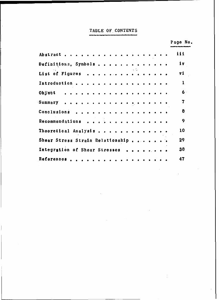
TABLE OF CONTENTS
Page No.
A b s t r a c t * .o . . . . . • . e e. o o * e & e
Definitions, Symbols.. . . . . . . . . . o . iv
List of Figures . . .O . . . . . * . . * . * vi
Introduction . . . .* a a * 0 0 .0 0 0 a * * 0 1
Obje#tt . . .o .* .* . . . . . . 0 0 & a 6
.Summary . . , . . . • . . o 0 , • • .0 . , * 7
Conclusions ., . .0 a 0 a .0 0 0 0 0 0 0a 0 8
Recommendations . . . o. * e a o o o a 9
Theoretical Analysis . . . . . . . . s * * 10
Shear Stress Strain Relationship . . .9 , o 29
Integration of Shear Stresses * * o a e, o * o 38
References. .. ...... * a 0 0 47

ABSTRACT
This report presents the first semi-empirical sol-
ution suggested to describe the traction versus slip
relationship for rigid wheels.
The kinematics of a slipping wheel are analyzed and
the results are used to express the shear deformation as
a function of slip which in turn is utilized in a new shear
stress-strain relationship. The shear stresses are express-
ed at every point of the tire-soil interface surface and
integrated to obtain the traction.
Other established information is also briefly dis-
cussed, in order to complete the description of the state-
of-the-art.
iii

DEFINITIONS, SYMBOLS
R Motion Resistance (Lbs.)
N Normal Component of the Resultant Soil Reaction (Lbs.)
T Tangential Component of the Resultant Soil Reaction (Lbs.)
Central Angle Associated with the Resultant Soil Reaction (o)
W Vertical Load on the Wheel Axis (Lbs.)
D Diameter of the Wheel (in.)
Mb Moment Due to Bearing Friction (inch Lbs.)
Factor of Bearing Friction
z Vertical Distance between a Point on the Wheel Perimeterand the Undisturbed Ground Level (in.)
z 0 Sinkage of the Wheel (in.)
0 Central Angle Associated with Z (o)
p Pressure (stress) Normal to the Boundary (Lbs./in. 2 )
kc Cohesive Modulus of Sinkage (Lbs/in. n+1
k Frictional Modulus of Sinkage (Lbs/in.n+2)
n Exponent of Sinkage
O( Central Angle Associated with Z
8 21 -
M Net Torque Applied to Drive the Wheel (inch Lbs.)
DP Drawbar Pull, Net Traction (Lbs.)
Vs Velocity of Slipping (in./sec.)
10 Slip
V t Theoretical Velocity of the Wheel (in./sec)
iv

W Angular Velocity of the Wheel (Rad/sec)
V Horizontal Component of the Velocity Vector at A Pointx on the Wheel Perimeter Associated with V = wt (in./sec)
V Vertical Component of the Velocity Vector at a Point onY the Wheel Perimeter Associated with V uit(in./sec)
C Instantaneous Center of Motion
r Rolling Radius (in.)
Y4 Ordinate of C (in.)
I Unit Vector in X Direction (in./sec)
j Unit Vector in y Direction (inJdsec)
' Angle Enclosed by the Velocity Vector and the X Axis (o)
1 v Central Angle Associated with the Point of the Wheelat which the Velocity Vector is Vertical.
a Acceleration Vector (in./sec )
SRadius of Curvature (in.)
sa Shear Strength of the Soil (Lbs./in. 2)Smax
c Cohesion (Lbs./in. )
Angle of Internal Friction
£2f Angle of Failure (o)
2s Shear Stress (Lbs./in. )
J Shear Deformation (in.)
K Tangent Modulus of a Shear Stress Strain Curve (in.)
V

LIST OF FIGURES
Figure No.
1. Equilibrium of a Towed Wheel.
2. Equilibrium of a Towed Wheel and Definition ofAngles c and F^,
3. Definition of Angle E.
4. Definition of x and x for Presenting theSimplifications in Bekker's derivation.
5. Equilibrium of a Driven Wheel.
6. The Path of a Point of the Wheel Perimeter.
7. Geometric Representation of the PeriphericalVelocity Vector.
8. Four Significant Velocity Regions on the WheelPerimeter.
ea. Velocity Vector in Region 2.
9. Velocity Vector Representation for Zero Slip.
10. Representation of Velocity Vectors for NegativeSlip.
11. Center of Curvature of the Path of a PointLocated on the Whee~l Perimeter.
12. Triazial Test Specimen and Mohr's Circle.
13. Mohr Circles for Various Principal Stresses.
14. Shear-annulus.
15. Typical Soil Shear Stress-deformation Curve.
16. Soil Shear Stress-deformation Curve with a Hump.
vi

Figure No.
17. Definition of "K".
18. Variation of "K" as a Function of the NormalPressure.
19. Surface Element of a Wheel.
20. Approximative Representation of a Wheel.
21, Shear-deformation J2 for a Wheel Which Sinksso that 1
22. Shear-deformation j for a Wheel shown inFigure 21.
23. Shear-deformation J3 when A cosl(1 - i )
24. Connection between Eo and /•_
vii

INTRODUCTION
The problems related to rigid wheel behavior in soft
soil were first analyzed by Bernstein (I). He derived re-
lationships between the load on a towed wheel of given geom-
etry and the sinkage as well as the motion resistance. The
basic assumption employed by Bernstein was that the normal
soil stress acting on the wheel surface is proportional to
the square root of the vertical distance of the point in
question and the ground level. Thus, the influence of the
soil on the stress distribution was accounted for by a factor
of proportionality (k). Russian agricultural engineers have
introduced another "soil characteristic" by using a general'
exponent (n) instead of the square root. (2). Most of the
Russian publications, however, follow Gerstner by assuming
n = 1, to avoid mathematical complications which arise from
the non-integer exponent. In 1950, Garbar (3), published a
very useful paper in which he suggested some new notions such
as the "critical inflation pressure".
A further development in the adaptability of the empir-
ical pressure distribution equation was accomplished by
Bekker (4), who suggested a new factor of proportionality which
is practically independent of the size of the penetrometer
footing, or 'that of the wheel-soil interface if the aspect

ratio is not allowed to be less than 5:1. Bekker rederived
(5)Bernstein's equations using the new soil value system
Vincent (6) (7) osreVincent (6) , and more recently Ilegedus , observed
some new relationships as to the normal pressure distribu-
tion under a wheel, but no method has been devised as yet to
describe it analytically.Tanaka (8) (9n)hllp
, and Phillips , analyzed the equilibrium
of wheels in their presentationsat the First International
Conference on the Mechanics of Soil-Vehicle Systems. Both
of the authors included the tangential forces, hitherto
neglected.
Uffelmann conducted tests (10) by means of a special
apparatus enabling him to measure the tangential "rim
stresses" and suggested a simple plastic theory of rut forma-
tion providing an estimate of rolling resistance. Ills equa-
tions are equal to Bekker's equations for zero exponent, or
in other words, they are valid for bearing capacity estima-
tions (zero sinkage). Therefore, no conclusions as to the
sinkage may be obtained on this basis.
An excellent analysis of the equillbrium of wheels by
Schuring also stresses the importance of the tangential
forces (11). In addition, it dwells on the possibility of
using dimensionless analysis techniques for the wheel pro-
blem.
2

The latter approach has also been elaborated on by
Hicks and Nuttal at the First International Conference
(12 and 13).
The kinematics of a rigid wheel and that of a soil
particle were analyzed by Andreyev() , and other Russian
investigators in great detail. Their basic assumption,
however, that the displacement of a soil particle and the
force acting on it are collinear is incorrect and leads to
certain ranges on the wheel perimeter according to slip
conditions which are questionable on the basis of test re-
sults obtained by Vincent and Uffelman4./ As for soft tires,
Omelyanov's empirical equation for resistance prediction is
(15)frequently published in Russian textbooks
Another Russian paper by Ageykin (16), reveals an equa-
tion for sinkago similar to that published by Bekker and the
writer (17, 18, 19, 20)
Experiments by the National Tillage Laboratory (21), by
the Waterways Experiment Station of the Corps of Engineers,(22) (2)
U. S. Army , by Soehne , and by a group consisting
of researchers from the National Tillage Laboratory and(24)
Michigan State University , elucidated some important as-
pects of the pressure distribution under soft tires operating
in deformable soils.
3

Ker(25) (26)
Kerr , and Chapoux , carried out extensive
research projects on tire behavior in sand. Weinblum and
Orlowski (27), as well as other Israclian researchers are
also engaged in investigating wheels in sandy soils.
They found that an exponential expression is suitable to
describe the traction slip relationship. Soehne and Sonnen
(28) arrived at the same approximation in their broad ex-
perimental studies presented in Turin. They emphasized the
difficulties which arose with the application of the Bekker
soil value system in multi-layer soils.
Turnbull and Freitag accounted for a massive tire test
program which is being conducted at the Waterways Experiment
(29)Station ( The authors investigate the change in per-
formance due to multiple passes, beside the traction-slip
problem.
A new, radial ply, tire design, introduced by the Pirelli
Company (30) proved to be superior to the conventional one,
according to tests conducted by the Company itself, by the
National Tillage Laboratory (311, and by the Ford Motor Co.
Bekker's condual tire concept appeared to be promising,
in view of theoretical considerations and some limited test
(33)results . Richey suggested the mounting of a radial ply
tire on a narrow rim. The idea proved to be advantageous(32)
over a conventional rim equipped with a radial ply tire
d

Various aspects of tire behavior on hard ground have
been analyzed by a great number of researchers and in-
stitutions. An excellent, If not quite up-to-date, digest
of these studies has been published by Hadekel( 3 4 ).
5

OBJECT
The purpose of this research project was the establish-
ment of simple equations based on empirical soil stress-
strain relationships which would enable one to predict the
sinkage, the motion resistance, and the traction of a rigid
wheel and a soft tire. While there have been empirical sol-
utions suggested for the first two problems, the question of
traction of wheels has not been evolved farther than the
statement that the tractive force is the sum of the horizon-
tal components of the stresses acting along the soil-wheel
interface surface. A number of researchers have stated that
a rigorous solution represents an impossible task at present.
This is probably true, since the basic theory of soil mechan-
ics has failed to answer such basic questions as the true
stress-strain relationship prevailing under a plate. No
wonder that a solution for the involved three-dimensional
problem of a tire-soil interaction, in which the behavior of
the carcass, and the effect of the lugs(35) represent even
further obstacles in the analysis, has not been considered
obtainable. Nevertheless it is felt that adequate empirical
knowledge is available on soil behavior to make our goal
feasible.
6

SUMMARY
Exact equations of equilibrium for driven wheels oper-
ating in soft soil are presented for which a formula for
motion resistance is derived.
Next a detailed analysis of the kinematics of a slip-
ping wheel is presented and a geometric representation of
the velocity distribution is introduced.
An empirical soil shear stress-deformation equation
is proposed. This equation is then combined with the re-
suits of the previous analysis and an equation for the gross
traction of a tire is derived.
7

CONCLUSIONS
The theoretical investigation leads to the following
conclusions:
The perimeter of the wheel may generally be divided
into four regions depending on the direction of the velocity
vectors that belong to the pertinent points.
When the sinkage is such that the region characterized
by vectors pointing forward and downward is a part of the
wheel-soil interface (in case of driven wheels) the tan-
gential stresses result in resisting forces. Hence, optimum
traction is reached when the sinkage is not greater than
the height of the point to which a vertical velocity vector
belongs.
B

RECOMMENDATIONS
It is recommended that the theoretical method presented
in this paper be thoroughly checked by a series of experi-
ments to establish its applicability and its limitations
9
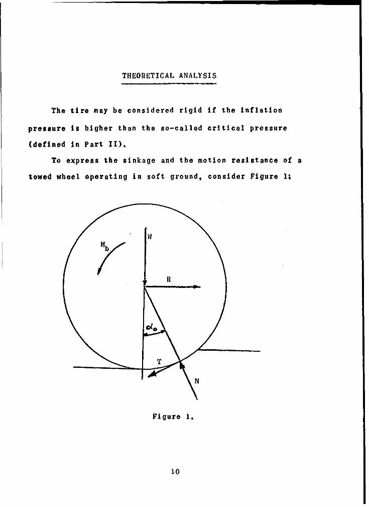
THEORETICAL ANALYSIS
The tire may be considered rigid if the inflation
pressure is higher than the so-called critical pressure
(defined in Part II).
To express the sinkage and the motion resistance of a
towed wheel operating in soft ground, consider Figure 1I
bR
Figure 1.
10

It is assumed that the problem is two dimensional.
The equations of equilibrium are the following:
R - N sin c>( + T cos w = 0 .. . .. l-a)o 0
W + T sino< 0 N cos 0o .(l-b)
T-D=0 .= (-c)2 b
where Mb = y naturally,
Thus, the magnitude of T can be found if W and 9 are
known. (Equation 1-c). The tangential component of the re-
sultant is a function of slip. This relationship will be
derived on page 38. Thus, it is theoretically possible
to establish the magnitude of the negative slip which occurs
under a towed wheel.
Figure 2.
11

Equation (1) may be rewritten as follows:
Ri d T cosovC - dN sinoC 0 . . . (2a)
0 0
W- dN cosoC.+ d T stnOC- 0 . . . (2b)
0 0
4J T - Mb 02 b
0
Thus, if dT = f (0c) and dN g (C) is known the sinkage and
%he motion resistance may be found.
Note that:
= 4(1 - coso) " " .*. . * ° (3)
Bekkers approximative equation will be used throughout
this paper for:
dN = f(z) = gK) h (0)p = dA
p = k k)e + k)cos 0 - cos )
* .. . . . .S (4)
z z0
Fig. 312

If one assumes that Mb is negligible, then T 0
and
R = 0 dN sin X rAN sin 0 . (5)
Using equation (4):
R D = (LC_ k_) S (Cos 0 - Cos '' n sin e dO2 b 2T 2
!c+kn+ Cs n+1
bj 2)() [ P 07 n + I
From equation (4):
1 - cos ,o -2
Thus:k + b k
n + 1 1
Equation 6 was first derived by Bekker(5), using energy
considerations. It enables one to approximate the rolling
resistance of a towed wheel for small slippages only because
the tangential forces have been neglected.
13

Fig9. 4
Bekker and Hegedus have attempted to remedy this short-
coming by introducing the so-called bulldozing resistance.
(5) (37).
Equation (2b) cannot be solved in a closed form even if
one assumes dT 0 for all A. Bekker has performed the in-
tegration (5) by neglecting the difference between x and x ,
(Fig. 4) and by considering the first two terms in the bi-
nominal series of
[1 - (Zo - Z)]
Ehrlich (36) improved-the accuracy of Bekker's solution
by considering three terms in the series. He found that the
accuracy is a function of n. Bekkerts solution yields the
following equation:
14

2
Zo -n) (k + bk
Since n • 2, according to actual measurements, n 3 is
excluded by practical considerations. Erhlich's equation
reads as follows: 2
20 bk~D 2nýl [0-.51 n+.22n 2) (.2 5 -2 6 n-1 4 1 2
"2--2( w ) I 2n+l(bk= • W-•51n +.22n2 2 n+lJ .
Equation 1, may be rewritten for a driven wheel as follows:
(Figure 5);
2T 21TSdT cos 0 + S dN sin 0 - R = 0 . . . (9-a)
2T -30 2rr-/3
21T
W + 5 dT sin 0 - 52n dN cos 0 0 . •.(9-b)
M - . 2n dT = 0 . . (9-c)2 S2T1 -0
dTdN
Figure 5.
15

Here R is called the drawbar pull (DP), and dN sin 0
is considered to be the motion resistance. Later it will
be shown, however, that a part of dT cos 0 is a resisting
force also in many cases.
In order to evaluate dT as a function of H, one has to
analyze the kinematics of a rigid wheel.
KINEMATICS OF A RIGID WHEEL
D _
Figure 6.
16

As the wheel moves from position 1 to position 2, while
turning by an angle O-point, "P" is transferred to "P", Fig.
6. The path of the point is called a cycloid and Its para-
metric equation is the following:
X -ý (0 - sin 0) . . . . . . . . . . . . ( 0a)
y ( - cos 0) .0......... (lOb)
Equation 10 is valid if no slip occurs between the hori-
zontal plane ( x axis) and the wheel perimeter. In case of
slip FP" is no longer equal to (D/2)E.
The relative velocity between the fixed x axis and the
bottom of Ahe wheel (v s) determines the slip as follows:
vosT* * . . * * * (11)o T
It can be seen that i 0 is positive if vs and vT are
of opposite sense (driven wheel). The theoretical velocity
(VT) is defined by:
D DVT .= 2t . . . . . . . (12)
Thust
S2 +V t 2 o vT t2P - s 2 0 - Ti
D ( i0
17

Thus, the equation of the path becomes:
X R [0 (]-i) - sin 0] . . . . . . . (14a)2 0
D (I - cos 0) . , (14b)Y 2
Denote Dr -(1-(I-i) ........ ** * ... (15)
2 o
Then 0xTh- rO - sin 0 . . . . . (16a)
D2 ( - cos 0) . . . . . . (16b)
or using
x - Jt(1 - i) sin (wt)] 1 * , (17a)
y D/2 (I - cos wt) . . . . * * (17b)
or D-- rut"j - sin (wt) . . . . . . . . (iBa)
y 1)12 (I - cos wt*) .. . . . (06b)
The parametric equation of the velocity vector is:
° (1x D - IvX d = -2 [(l - i w - cos ct)] i (19a)
• D
v-d-L -- 2 sin wt * (19b)1y dt 2
V x wr 2 t] .......... (0
16

When C0 wt 0 or 2 T
vx =. w(r - D/2) = -1D/2 i -v T i 0 V * (21a)
vy = 0 . . . .. . . (21b)
Thus at the bottom of the wheel, the velocity is equal to v
The speed or the absolute value of the velocity is:
*2 L i2•(2-x + yw sin (M- t)(l - i )+ 2 ]s p 2 2 0 o+i0 (2
F o r i 1 -- 2
For i 0: v { : Dw'sinl t) . . . . .. .. (23)
Imagine that the entire xy plane is rigidly attached to
the wheel. There exists a point in the plane where velocity
is zero. This point is called the instantaneous center of
motion (C). It can be seen that C must lie on the vertical
line of symmetry. (Equation 21). Every point in the revolv-
ing and translating plane may be thought of as being on the
perimeter of a wheel of radius (D/2)". From Equation 20:
v = w[r- (D/2) J 0
when (D/2) = r - D/2(1 - i ) . . . . . . . . (24)
Thus Yc D)/2 - D/2(1 - i 0 = 1)/2 io .. ....... .. (25)
19

Hence, r (1 - i ) D/2, is the radius of an imaginary0
wheel which is attached to the actual wheel and has no slip
at its bottom, which is at C. D/2(0 - i ) = r, is often
called the rolling radius.
In case of driven wheels, vs <0. Thus, 10 >0, r 0/2,
and yc >0, which means that the instantaneous center is above
the x axis. For 0= 1 (100% slip), r = 0, or yc = D/2. Thus
C coincides with the center of the wheel. For towed wheels,
vs >0, 10 (0, r >D/2 and y c <0
since r =D/20 + i.01 ). . . . . . . . . . (26)
C is below the x axiL.
For i = I.100% negative slip)0
r = P D/2 = D
Consequently, i0 - -100% does not represent a complete-
ly blocked wheel. When io , VT 0, r -4 c, or y -
which means that the wheel slides on the ground without turn-
ing. (When VT--4 ., w---o, since vT = wt). It is not advis-
able to use two different definitions for the slip, as is
generally done, dipending on whether one deals with driven
or towed wheels, :)ecause the mathematics cannot be kept com-
pletely general. In other words, if one defines negative
slippage so that it becomes-l00% when the wheel is blocked,
so that v
I ( - 5
VT + V
20

then the case of towed wheel cannot be handled with the same se±
of equations derived for driven wheels.
An interesting geometric representation of the velocity
vector distribution along the wheel perimeter is presented
in the following. Construct a circle of radius D/2w so that
the abscissa of its center be x ru, = D/2 (1 - 0 )w and
its ordinate be zero, Figure 7.
Av
21

The velocity vector associated with an arbitrary point
A on the wheel perimeter can be found as follows:
a. Connect A and C
b. Draw a line perpendicular to AC through 0
The line segment 6-W represents the velocity vector at
A.
Proof: -A A (rw + D/2 w cos ) T + R w sinft
but Cos -Cos -cosl0
sin/ = sin 0
Figure 8
Hence TA (rw - D/2 w cos 0) T + D/2 w sin 0 j . (27)
22

Equation 27 is equal to equation 19 or 20, Q.E.D. (To
see that 0 8 11 consider the triangles AO'C and O0"At.
Two of their sides are proportional, D/2, r and D/2 , rr
and one of their angles is equal.llence the triangles are
similar, thus all three angles are equal).
It can, therefore, be concluded that the circle con-
structed is the hodograph of the path.
DRIVEN WHEELS:
The wheel perimeter may be divided into four regions
according to the "behavior" of the velocity vectors.
Region The velocity vectors point up and to the
right along Section 41 (Fig. 8).
iu 0
Figure8a. z

Region 2: The velocity vectors point downward and to
the right on Section 12 Therefore, if the sinkage of the
wheel z is such that zO> Yc positive horizontal deformation
and compaction is imparted on the soil along the section as-
sociated with z0 - Y., The point on the wheel perimeter
whose ordinate is yc belongs to an angle 9v = coil(1 - 1o))
because (from Equation 19a) vx o when wt 8 = - 0
Thus, the region characterized by z0 - Yc may also be defined
as follows: 221r - P •0 •0 ý
or from Equation 3:
2z
2 C - cos 1 (1 -D----) < 0 • cos(1 - 1o)
The tangential forces acting on the wheel in Region 2
have negative horizontal components, thus an additional re-
sistance will occur. The sum of these tangential forces has
been denoted H2 (38). Note that Region 2 is I'mportant only
when 2r - to h Ev = cos0 0 - io)
Thus, the sinkage and the slip has to satisfy the above
inequality when H2 O.
Region 3: The velocity vectors point downward and to
the left along Section 23 Compaction and positive horizon-
tal shear stress components occur here when the wheel is
driven. The s3ction of the wheel perimeter along which
24

positive shear stresses (tractive forces) occur is defined
by ý3. When 27T-o 0 Ov this section becomes the entire
arc 23
Region .4: Here the velocity vectors point upward and
to the left. Neglecting the small recovery effect of soils
this region is of no importance, since the wheel is not in
contact with the ground along arc 34M
Zero Slip: For zero slip, r = D/2(0 - i ) = D/2. TheS~0
hodograph is tangent to the y axis. (Fig. 9). (C is at 0).
There Are no velocity vectors with negative horizontal com-
ponents. Hence, traction cannot be developed.
LY
BBtB* jo- x
Fig. 9
2 5

There are two regions only. The velocity vectors along OB
point upward and to the right, while along BO the vectors
point downward and to the right.
Negative Slip: For negative slip, the diagram is shown
in Fig. 10. There are two regions as in the no-slip case,
but v = v at the bottom of the wheel.s
2
A
""2 0
Fi(. 10
26(

Acceleration:
The acceleration of a point located on the wheel per-
imeter may be obtained from Equations 19a and b.
°° d2x 2v
a .x = 2 dt - D/2 w sin wt (2 8 a)a x dd-
2 dv = 2 (28b
_ ~ w D 2w Cos wt *dt2 dt D/2 t (26b)
Note that the acceleration is independent from the
slip. It can be seen that the endpoints of the acceleration
vectors describe a circle of radius D/2 w The magnitude
of the acceleration
[ = a 4 2 y2 = D/2 w 2 is constant.
Its direction is parallel to the radius and its sense points
toward the center of the wheei, just is in the case of a uni-
form circular motion.
The radius of curvature is:
(k2 4 k2)3/2
S(29))
x y
x ..
Fo rio : • : B sin (2 t) . . . ... . . .. (. .
2 _= _ CJ~:j7
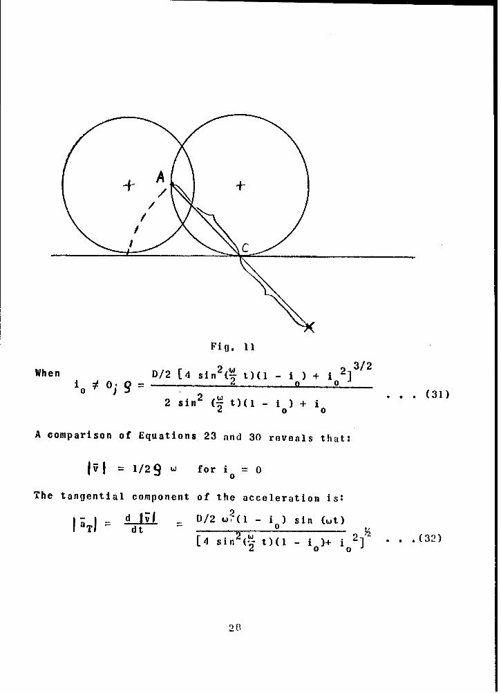
Fig. 11
When D/2 [4 sln 2 (0 t)(1 J 0 32
10 i 0 2w . , (31)
2 sin( t)(2 - i ) + i0 0
A comparison of Equations 23 and 30 reveals that:
IV I = 1/29 w for i° = 0
The tangential component of the acceleration is:
laT d 1;1 D/2 20( - ) sin (w•it)
dt 26 t 1 )+ i 2] (32)[4 sin -t-
28I

for 1 00
( a T = / 2 w 2 c o s 0 ~ - t ) * * * * * * * * * * * ( 3
for i 1
00
The normal compo'ent of the acceleration is
D 2 2 1tL !INw1 2 sin4 2 ol I
2 sin 2 (W t)(1 - to) + io21
for 00 00
1a~ 11 sin (_ t) 6 * 0 0 0 0 (35)
for i 1
0
N1 27 -
From Equations 32 and 34
2 2a J + 2 ' T W (36)
This checks with Equations 2Oa and b. Thus, when the wheel moves
with constant speed w = const) the acceleration vectors are not
different from that of uniform circular motion.
SHEAR STRESS STRAIN RELATIONSIIIP
The next task Is to establish a shear stress-strain re-
lationship which allows one to describe an experimental soil.
29

shear curve by means of coefficients, which depend on the soil
and its state. (Moisture content, density, load history, etc.).
The soil shear strength was first expressed by Coulomb(39)
as follows:
Smax, c + p tan $ . ... . . . (37)
The numerical values of c and • may be obtained by tri-
axial tests or by direct shear test. The well known triaxial
test procedure is as follows( 4 0 ). A cylindrical soil speci-
man is subjected to p, axiol stress and P3 radial stress.
Mohrils diagram, Figure 12, represents the stresses act-
ing on a plane which inclosed (I - ( ) angle with the axis2
of symmetry.
P P
30

When failure occurs the shear stress reaches the shear
strength in the failure plane, according to Coulomb's cri-
terion. Thus, S max has to satisfy the equation of Mohr's
circle and that of Coulomb's straight line (Equation 37).
Thus,-smax 2 sin = c + p tan ..... 0(38)
(Here p1 and p 3 are the stresses applied at failure).
Since +
2 +
F 4 2 for the failure plane.--2 F= '4 + 2
Thus, 0 can be evaluated when .F is known.
From Equations 38 and 39:
sin (-2 + c) C + pF tan (40)22F
orPl - P3 Cc, 1 tan2 os , PFtn
and c = Pl 2- P3 csptn(12os$ - p tan $ ... . .. . .. (41)
The value of p, however, is still unknown.
31

From Figure 12:
PF P 3 + Pl P3 + 2 Cos22
PF I + p 3 ) + -s( + 3)
Thus, F = (P + P 3 )'(P- p 3 ) sin . . . . . (42)
Since it is difficult to measure OF, it is advisable
to perform two or more triaxial tests with various P3 values.
•of
P ------ f
0 39• '- --- P 3 " - - --*
Fig. 13S 9 66 II
Then, p, will vary at failure. By knowing p 3, Pl' P3 . Pls
etc., the envelope of the M.ohr circles (which actually ap-
proxima;lte% a straight line) may be obtained. Its angle of

inclination is 0 and its intercept with the s axis is c.
Since a triaxial test is a slow procedure, it is not suit-
able to obtain a large number of soil values in a short .time,
Therefore, quicker procedures have been devised. Bekker pro-
posed a shear apparatus in which a normal load and a torque
is applied on an annulus which rests on the soil surface (17,
41). Thus, the average normal and shear stress acting in the
horizontal plane directly under the ring (soav) can be re-
corded. The shear stress which is recorded at failure is
considered equal to max* c + p tan 0, where p is tte normal
pressure applied.
Actually, it is not evident that the failure occurs in
the horizontal plane. Thus, the recorded value may be a
shear stress value which acts in the horizontal plane while
failure occurs and s max may act in some other plane. Ex-
perimental evidence clearly shows, however, that the maximum
torque per annulus area reading is a linear function of the
normal pressure applied. The relationship may be expressed
by means of an equation similar to Coulomb~s.
smax = cB + p tan B . . . . .. . (43).
Figure 14.
33

Here index "B" stands for "Bekker's coefficient", as
opposed to Coulomb's cohesion and friction angle. The
relationship between CB and c, as well as between 0 and Bf
is not clear as yet. Since cB and 0B is more suitable to
describe vehicle operation in soft soils than c and $, Land
Locomotion Mechanics studies use the former sets of param-
eters. Thus, c B and 0 B will be used and index "B" will be
dropped henceforth.
An experimental shear stress-strain curve is of the
shape shown in Figure 15 in most cases. Sometimes a hump
and decay occurs as shown in Figure 16:
•S"S
Figure 15. Figure 16.
Bekker introduced an empirical equation, similar to that
derived for an overdamped one degree of freedom spring-mass
system and proposed two additional soil values (K 1 and K2 ) to
replace the damping and the natural frequency of the undamped
34

(5)system W Weiss constructed a nomogram which enabled one
(43)to evaluate K1 and K2. 2 Practice has shown, however,
that the hump bears no practical importance because it occurs
only at certain undisturbed clay soils which are not surface(44)
materials . Furthermore, the effect of a hump may be
neglected In the integration of shear stresses over a solid
boundary because the deformations associated with the hump
occur only under a relatively small part of the soil-vehicle
interface surface. Experiments show that the hump decreases
and finally disappears as p increases. When the curve is
similar to that shown in Fig. 15, the following expression
lends itself to replace Bekker's equation:
s s s (1 _ ;j/K) . . . . . . . . (44)
Equation 44, cannot be derived by a limit process from
Bekker's equation unless some approximative assumptions are
made!45). Similar relationskips were arrived at by Nuttal
(13), Soehne (29) and Weinblum (28).
The physical meaning of K can be seen in Fig. 17. Ac-
cordingly, K is the abscissa of the intersection of the
S
s
Fig. 17
35

curve (s= s max) and the tangent drawn at the origin
Since (ds) = max
the equation
ds j= o max
is satisfied when K = j. Thus, K is the abscissa of the
point described above.
Therefore, one can obtain the numerical value of K by
drawing the tangent at the origin and finding its intersect
with the asymptote.
Reece suggested another method to evaluate the numer-
ical value of K in his discussion of Paper No. 41 at the
First International Conference on the riechanics of Soil-
Vehicle Systems. (Also see Ref. 45). lie reasoned that if
r
flax.
then s 0(lthn log(_S - 1) = -
Smax. ,
So the log of -1- -l is proportional to J. (The factorSmax
of proportionality being 1). Therefore, If one plots(-) ~inn7 X",
- )on a logarithmic axis and j on a linear scale, K will
represent the slope of the straight line j - og(- 1)M ax
36

Equation 44 only approximates a true shear curve, hence
one seldom obtains a continuous straight line when replotting
the experimental shear curve on a seri-log paper. Therefore,
the argument for Reece' s method emphasizes that one is free
to consider a larger portion of the curve than the initial
one which is often not clear]y definable.
Next, the question arises as to how K is influenced by
the normal load (p), the diriensions of the Bevaeter annulus
and possibly somIe other factors. In other words, does K
solely depend on the soil and its state? It is most likely
that this is not so. A limited number of test results ob-
tained at the Land Locomotion Laboratory seem to indicate
that K is proportional to the circumterence of the annulus.
K also increases with the normual pressure, but it becomes
constant when the normal pressuire surpasses 3 - 4 psi.
S• •.--P = 3.5 psi
-J
I,'ig•. 10
37

J. Adams(45) investigated this problem in his Master's
Thesis completed under the supervision of A. Reece. He
found that K is proportional to smax * lie recommended the
following equation: K s . -- max*
s max(l-e )
Here K refers to the tangent modulus measuredat max = 1
lb/in2 o In his experiments, shear tests were carried out
by a shear block and not an annulus and the "semi-log" tech-
nique was used instead of the "tangent method" to evaluate K.
It is stuggested that a broader investigation is required to
elucidate the true nature of the various effects which in-
fluence K.
INTEGRATION OF SHEAR STRESSES
The term 1l 2v dT cos e (Equation 9 -a)
2nr - P
is analyzed in the following. ClearlylD
dT s b -d . , .d , , (45)2
D CI
Figure 19.
38

or by Equation 44
dT =S( - ej/K bD= s ( dO . . . . .(46)
From Equation 43:
dT = (c + p tan 0)(l - ej/K) b-- dO . . .(7)2
Thus
b D (c + p tan C) - -i/K) cos 0 dO . .(48)
2w
The next problem is to relate j and 0.
If one approximates the wheel as shown in Fig. 20, then the
following-assumptions may be made.
Fig. 20
The horizontal component of T is a function of the normal
pressure prevailing at z and the horizontal component of the
total deformation. The annulus sinks into the ground duringj
39

a shear test but only the horizontal deformation is recorded.
The soil values obtained correspond to horizontal deformation
components. Another question to be cleared with respect to
this problem is the following. The normal pressure is vary-
ing from zero to p. The assumption that the shear stress
created is the same as measured under p - constant may not
be true.
According to Figure 21, the deformation at e is
=2 dx S a dx dO . . . . (49)J2 X2T-PO 21T- P3O d
From equation 14 a:
=9 d Eu - o0 0)] (50)
Thus, D 0J2 2 S [(1 - 1) -cos 0] dO . . (51)2ff- Po
When 2n < OS21.cos -) - (Region 2).
Hencej D - 10M(o - 2n - sin 0 - si .(52)
40

yN
$6il Level
Figure 21.
As E) becomes' greater than cos (i -i ), Region 3, the0
direction of tre deformation changes and a negative j will
be generated (Figure 22). In order to maintain a negative
exponent in Equation 40, j has to be obtained for:
21T - o 2,cosl(1 - io) < 0 • 21 as shown below:
-1d dX 27r-cos (1 - i ) (djl= -5 -.. dO =.S 0 d
-I dO dOZr.cos (1 - i 1
", 11

Wheel
coil(1-to)
S .oil Level
t • C Vertical Tangent
-- l~ ---- •
Fig. 22
or
J [( - io)( -O0) - sin ) + sin 9. . . .• (54)
j=2w-coi 1 (l - i ) . . . . . . . . (55)
The sum of the shear stresses along the soil-wheel in-
t e r f a c e b e c o m e s : H = H - . , .* , , , . . , . ( 5 6 )
42

where 2w e e HbD 2 y/K) d( 71 2 f (c + p tan 0)(1 - K d 0 .... (57)
v
4V j2/K
H bD f (c + p tan WI)(l - e ) d 0 * .(50)2 = 2
Equations 56, 57, 50, 54 and 52, allow ,,one to evaluate
the traction of a wheel when the sinkage is larger than yc"
In other words, when the sinkage is deep enough to cause
soil-wheel contact along that region of the wheel perimeter
(Region 2) whose points move forward and downward. Using our
notations, Equation 56 is to be used when 0o 2W. - 0 ,.
When /3, 2* - 0, only Region 3 has to be considered.
y
Vertical Tangent
Fig. 23
43

Figure 24.
Here, Figure 23:0 dx dO
where 9v 2 • - 13, < 0 2y
"J3 2S To- dO= 2 (1 i )(2- 0
+ sin ,+ sin 0] . . . . . . . . . . (59)
44

j 3Thus bD 2T -- KT = bD -- r (c + p tan 1 )(1 - e ) dO . . . (60)
2Tr -f
Equation 60, yields the tractive force when (See Equation 3):
2zocosl(1 - i) 0 = colo(1 - -)
Before Equation 56 or Equation 60 can be programmed for
an electronic computer, p has to be expressed as a function
of 0.
Equation 4, yields the expression desired:
k D np b ( + k [(cos 0 - Cos0) (4)
The foregoing method may be summed as follows:
1. Find z (Equation 7)0
2. Find (?o (Equation 3)-o 1 -
3. Find 0 v o -
4. If A > 2n - 0v (Use equations 4, 53, 54,
57, 58 and 56 to find H)
5. If o 2n - 0v (Use Equations 4, 59 and 60)
6. Subtract R (Equation 6) from H1.
45
The following input data are necessary to perform the
Calculationst k , k6, n , c, 0, K, D, b, IV, io. The
variable is E naturally.
46

"REFERENCES
1. Bernstein, R., "Probleme zur Experimentellen MotoroflugMotorwagen, 1913.
2. Goryachkin, V. D., (collective work), "Tedria i ProsivodstuvoSielskohoziayniti Mashin", Moscow, 1936.
3. Garbari, F., "Resistenza al Movimento Dei Veicoli a Routeso Terreno Cedevole", Ata, Rendiz Congr. 9-11.
4. Bekker, M. G., "A Proposed System of Physical and GeometricTerrain Values for the Determination of Vehicle Performanceand Soil Trafficability", Interservice Vehicle MobilitySymposium, Office of Ordnance Research, Duke Universityand Stevens Institute of Technology. Published by LandLocomotion Research Branch, OTAC, Detroit, 1955.
5. Bekker, M. G., "Theory of Land Locomotion", (Chapter VI),University of Michigan Press, Ann Arbor, Michigan, 1956.
6. Vincent, E. T., "Pressure Distribution On and Flow of SandPast a Rigid Wheel", First International Conference on theMechanics of Soil-Vehicle Systems, Turin, 1961.
7. Hegedus, E., "A Preliminary Analysis of the Force SystemActing on a Rigid Wheel", Report No. 74, Land LocomotionLaboratory, OTAC, Detroit Arsenal, Centerline, Mich., 1962.
8. Tanaka, T., "The Statistical Analysis and.Experiment on theForce to the Tractor Wheel", Paper No. 18, First Inter-national Conference on Research and Engineering Mechanicsof Soil-Vehicle Systems, Turin, 1961
9. Phillips, J., "A Discussion on Slip and Rolling Resistance",Paper No. 54, First International Conference on theMechanics of Soil-Vehicle Systems, Turin, 1961.
10. Uffelmann, F. L., "The Performance of Rigid CylindricalWheels on Clay Soil", Paper No. 7, First InternationalConference on Research and Engineering Mechanics of Soil-Vehicle Systems, Turin, 1961.
11. Schuring, D., "On the Mechanics of Rigid Wheels on SoftSoil", (in German) VDI, June 1961.
47

12. Hicks, Ho. I., "A Similitude Study of the Drag and Sinkageof Wheels Using a System of Soil Values Related to Loco-motion", Paper No. 30, First International Conference onthe Mechanics of Soil-Vehicle Systems, Turin, 1961.
13. Nuttal, C. J. and McGowan, R. P., "Scale Models of Vehiclesin Soils and Snows", Paper No. 39, First InternationalConference on the Mechanics of Soil-Vehicle Systems, Turin,1961.
14. Andreev, A. A., "Analytical Treatment of Certain Problemsin the Kinematics of Wheels of Agricultural Machines",(in Russian), Sborn. Trud. Po Zemledel'chcsk, Mekh. 23-12, 1954 USSR.
15. Omelyanov, A. E., "0 Primenii Pneumatichenih Koles",Selhozmashina, No. 5, 1940.
16. Ageykin, Y. S., "Opredechenie Deformatsii ParametrovKontakta Shiny s Myagkim Gruntom", Autom. Trakt. Prom1959 (5).
17. "A Soil Value System for Land Locomotion Mechanics",Report No. 5, Land Locomotion Laboratory, OTAC, DetroitArsenal, Centerline, rMrich., 1950.
18. Janosi, Z., "Soil Values in Land Locomotion", Journal ofAgricultural Engineering Research, Vol. 5, No. 1, 1960.
19. Bekker, M. G. and Janosi, Z., "Analysis of Towed Pneu-matic Tires Moving on Soft Ground", Report No. 62, LandLocomotion Laboratory, OTAC, Detroit Arsenal, Centerline,Michigan.
20. Bekker, M. G., "Off-the-Road Locomotion", University ofMichigan Press, Ann Arbor, Michigan, 1960.
21. Reed, I. F., "Pressure Patterns for Conventional andRadial Ply Tires", Presented at the meeting of the ASAECommittee on Tractive and Transport Efficiency at theNational Tillage Laboratory, Auburn, Alabama, 1960.
22. Thompson, A. B. and Smith, M'. E., "Stresses Under MovingVehicles". Technical Report No. 3-5445, Report 2, U. S.Army Engineer, Waterways Experiment Station, Corps ofEngineers, Vicksburq, Mississippi, 1960.
48

23. Soehne, W., "Druckieriteilung im Boden und BodenverformungUnter Schlepperreifen", Grundlagen der Landtechnik, Vol.5, 1953.
24. Vandenberg,G. E., Cooper, A. W., Erickson, A. E., "SoilPressure Distribution Under Tractor and Implement Traffic",Agricultural Engineering, Vol. 30, No. 12, December 1957.
25. Kerr, R. C., "A Design Guide for the Application of Pneu-matic Tires to Vehicles Intended for Off-Road Service",Arabian American Oil Company, 1955.
26. Chapoux, E., "Pneumatic Pour Vehicles Sahariens", Engi-neur de l'AutomobilVol. XXXII, No. II, 1959.
27. Weinblum, Mand Orlowski, S., "Factors Affecting WheeledTractor Traction on Sandy Loose Soils", Paper No. 51,First International Conference on the Mechanics of Soil-Vehicle Systems, Turin, 1961.
28. Sohne, W. and Sonnen, F. I., "Rolling Resistance and Draw-bar Pull Measurements of Wheeled Tractors as well as anInvestigation of Soil Value Systems", (in German), PaperNo. 32, First International Conference on the Mechanicsof Soil-Vehicle Systems, Turin, 1961.
29. Turnbull, W. J. and Freitag, D. R., "Influence on SoilFactors and Tire Geometry on the Performance of PneumaticTires in Sand", Paper No. 31, First International Con-ference on the Mechanics of Soil-Vehicle Systems, Turin,1961.
30. Mazza, C. and Amici, "Essais sur Pneus Pour TracteursInfluence de la Structure de la Carcassee", R, G. C.,Vol. 36, No. 10, 1959.
31. Vandenberg, G. E. and Reed, I. F., "Tractive Performanceof Radial Ply and Conventional Tractor Tires", Paper No.61-608, Winter Meeting of ASAE Chicagoi, December 1961.
32. Richey, C. B., "Techniques for Field Test Comparisonof Tractor Tire Efficiency", Presented at the meeting ofthe ASAE Committee on Tractive and Transport Efficiencyat the National Tillage Laboratory, Auburn, Alabama, 1960.
33. Hegedus, E., "Evaluation of Condual Tire Model", ReportNo. 60, Land Locomotion Laboratory, OTAC, Detroit Arsenal,Centerline, Michigan, 1960.
49
34. Hadekel, R., "The M1echanical Characteristics of Pneu-matic Tires", Issured by T.P.A. 3, Technical InformationBureau for Chief Scientists, M1inistry of Supply, England,1944.
35. Trabbic, G. IV., "The Effect of Drawbar Load and TireInflation on Soil-Tire Interface Pressure", Mlaster ofScience Thesis, Michigan State University, Dept. ofAgricultural Engineering, 1959.
36. Ehrlich, I. R., "Wheel Sinkage in Soils", Ph.D. Thesis,University of Michigan, 1960.
37. Hegedus, E., "A Simplified Method for the Determinationof the Bulldozing Resistance", Report No. 61, Land Loco--motion Laboratory, OTAC, Detroit Arsenal, Centerline, Mich.,1960.
38. Janosi, Z., "An Analysis of Pneumatic Tire Performance onDeformable Soils", Paper No. 42, First International Con-ference on the Mechanics of Soil-Vehicle Systems, Turin,1961.
39. Coulomb, C. A., "Essai stir une Application de Maximiset Minimis a Quelques Problemes de Statique Relatifs aL'architecture, Mem. Div. Say. Academie des Sciences,Paris, Vol. 7, 1773, p. 343.
40. Terzaghy, K., "Theoretical Soil Mechanics", John Wiley& Sons, New York.
41. "A Soil Value System for Land Locomotion Mechanics",Research Report No. 5, Land Locomotion Laboratory, OTAC,U. S. Army, Detroit Arsenal, Centerline, Michigan, 1958.
42. Weiss, J. S., "Preliminary Study of Snow Values Relatedto Vehicle Performance", Report No. 2, Land LocomotionLaboratory, OTAC, Detroit Arsenal, 1956.
43. Goodman, L. J., "The Influence of Remolding or Disturbanceto Clay Soils on Mobility Problems", Syracuse UniversityResearch Institute College of Engineering, 1961.
44. Adams, J., "An Analysis of Tracklayer Performance", MSThesis, Agricultural Engineering Department, Universityof Durham, 1961.
50

TECHNICAL REPORT DISTRIBUTION LIST
DATE: JUNE 1963 Report No. 8091LL No. 8
PROJECT TITLE: PERFORMANCE ANALYSIS OF A DRIVEN NON-DEFLECTING TIRE IN SOIL.
Address Copies
Director, Research and Engineering Directorate (SMOTA-R) ... ..... 1
Components Research and Development LaboratoriesATTN: Administrative Branch (SMOTA-RCA) .......... ............. 2
Components Research and Development LaboratoriesATTN: Materials Laboratory (SMOTA-RCM) . . .. ........ ......... 1
Systems Requirements and Concept DivisionATTN: Systems Simulations Branch (SMOTA-RRC).... ......... 1ATTN: Systems Concept Branch (SMOTA-RRD) ...... ....... 1ATTN: Economic Engineering Study Branch (SMOTA-RRE) .... ....... 1ATTN: Systems Requirements Branch (SMOTA-RRF) ... ........ . .. . 1ATTN: Foreign Technology Section (SMOTA-RTS.2) ....... .......... 1ATTN: Technical Information Section (SMOTA-RTS) ...... ......... 2
Commanding GeneralU. S. Army Mobility CommandATTN: AMSMO-RR ...... ............... .................. 1ATTN: AMSMO-RDC ....................... ....................... 1ATTN: AMSMO-RDO .... ..................... 1Warren, Michigan 48090
USACDC Liaison Office (SMOTA-LCDC) .............. ................ 2
Sheridan Project Office (AMCPM-SH-D) ............ ............... 1
U. S. Naval Civil EngineeringResearch and Engineering LaboratoryConstruction Battalion CenterPort Hueneme, California ..................................... 1
Commanding OfficerYuma Proving GroundYuma, Arizona 85364 .................. . . ............ 1
Harry Diamond LaboratoriesTechnical Reports GroupWashington, D. C. 20025 ................................... 1
51

No. ofAddress Copies
Defense Documentation CenterCameron StationATTN: TIPCAAlexandria, Virginia 22314 ...................... 10
Commanding GeneralAberdeen Proving GroundATTN: Technical LibraryMaryland 21005 ............ ................ . . . . . . . . . . 2
Commanding GeneralHq, U. S. Army Materiel CommandATTN: AMCOR (TW) ...... ......................... 1ATTN: AMCOR (TB) .................... ......................... 1Department of the ArmyWashington, D. C. 20025
Land Locomotion Laboratory ................. .................... 2
Propulsion Systems Laboratory ............ ............... . . . 5
Fire Power Laboratory .................. ....................... 1
Track and Suspension Laboratory .............. ................. 6
Commanding GeneralU. S. Army Mobility CommandATTN: AMCPM-M60Warren, Michigan 48090 .................. ...................... 3
Commanding GeneralHeadquarters USARALAPO 949ATTN: ARAODSeattle, Washington .................... ....................... 2
Commanding GeneralU. S. Army Aviation SchoolOffice of the LibrarianATTN: AASPI-LFort Rucker, Alabama ............... .......................... 1
Plans Officer (Psychologist)PP&A Div, G3, Hqs, USACDCECFort Ord, California, 93941 ......... . ...... ................ 1
Commanding GeneralHq, U. S. Army Materiel CommandResearch DivisionATTN: Research and Development DirectorateWashington, D. C. 20025 ............... ....................... 1
52

No. ofAddress Copies
CommandantOrdnance SchoolAberdeen Proving Ground, Md......... . . . .... .
British Joint Service MissionMinistry of SupplyP. 0. Box 680Benjamin Franklin StationATTN: Reports OfficerWashington, D. C ........ . .. , . . . . . ° . . . ..... 2
Canadian Army Staff2450 Massachusetts AvenueWasHngton, D. C. . . ..................... . . 4
British Joint Service MissionMinistry of Supply Staff1800 K Street, N. W.Washington, D. C .............. • ........... 6
DirectorWaterways Experiment StationVicksburg, Mississippi ............. . ....... . . 3
Unit XDocuments Expediting ProjectLibrary of CongressWashington, D. C.
Stop 303 . . . . . . . . . . . . . . . . . . ... 4
Exchange and Gift DivisionLibrary of CongressWashington, D. C. 20025 . . . . . . . . . 0 a . 'a 0 . a 0 1
HeadquartersOrdnance Weapons CommandResearch & Development DivisionRock Island, Illinois
Attn: ORDOW-TB ..... . . . . . . . . . . ......... 2
Army Tank-Automotive CenterCanadian Liaison Office, SMOTA-LCAN ...... . . . . . . ... 4
United States NavyIndustrial College of the Armed ForcesWashington, D. C.
Attn: Vice Deputy Commandant . . . ..... e..... . . . . 10
Continental Army CommandFort Monroe, Virginia . ................ . ..... 1
53

No. ofAddress Copies
Dept. of National DefenseDr. N. W. MortonScientific AdvisorChief of General StaffArmy HeadquartersOttawa, Ontario, Canada ........... ................ . . . . . . 1
Commanding OfficerOffice of Ordnance ResearchBox CM, Duke StationDurham, North Carolina .................. ..................... 3
ChiefOffice of Naval ResearchWashington, D. C . . . . . . . . . . . . . . . . . . . . . . . . . 1
SuperintendentU. S. Military AcademyWest Point, New York
Attn: Prof. of Ordnance ................ ................... 1
SuperintendentU. S. Naval AcademyAnapolis, Md ...................... ........................... 1
Chief, Research OfficeMechanical Engineering DivisbnQuartermaster Research & Engineering CommandNatick, Massachusetts ......... ..................... . ... 1
Mr. M. BahnDepartment 6101Chrysler Defense EngineeringBox 1316Detroit 31, Michigan ................. ...................... 1
54

c, .1 I
V C. -C
M. L*4 a
L 0Sc L.w 0 )a..a - 1 4 '
C8 w 0o -0 . cW-
-O w4. -L 0b 0 f 14_j 2L Og 0 0)CLw~ UV 9.. - ,t 9 o b s
lb. 64. ii.0 o
L# 0 CL .0 4 0 - 44 a fL
50 ft O @4 . Cb ~~* U 4 O
o~. Z IL b C
It i IU LU C
WO ~ -SS I. £0 C £6* LE0 ~ £
-4 UW n o 0 .ON ~0:. I-. ~ ~ W
0 0
4! .- -
0.. w e4.',
. lp 0- a : .W4 .L -us 14. 4.4 4.. 0
WL c I-IL
tu. 0 41 a 0
j C1 j' Z a 4c 0CU 4.
IS . ~ !! t, I~
LA L c~~4 4. c. c
.5 IO U .4 4.I£0 ~ ~ ~ ~ _ i~C s W ~ ~ ~


