20 Simplicity, Complexity and Scale in Terrestrial Biosphere

20 Simplicity, Complexity and Scale in Terrestrial Biosphere Modelling

MICHAEL R. RAUPACH, DAMIAN J. BARRETT, PETER R. BRIGGS & J. MAC KIRBY

1. INTRODUCTION The terrestrial biosphere, encompassing vegetation and the adjacent soil and atmos-phere, is a biogeochemical crossroads where the interactions between energy, water, carbon and nutrient transfers are among the most complex that occur anywhere in the Earth system. These strongly coupled cycles are of fundamental significance in several disciplines: meteorology, climatology, plant physiology, agricultural science, ecology, remote sensing science, as well as ecohydrology and catchment hydrology. Models describing these processes are variously known as soil–vegetation–atmosphere transfer (SVAT) schemes, land surface parameterizations (LSPs) or terrestrial biosphere models (TBMs). We will use the last term. The motivating idea for this chapter is that hydrological prediction—including prediction in ungauged basins—is aided by incorporating information about energy, carbon and nutrient exchanges. This is true for both modelling and observational reasons. From a modelling standpoint, major terms in the water balance—principally but not only evapotranspiration—are biotically controlled and hence linked with carbon and nutrient cycles. A model which acknowledges these biotic controls is a better hydrological model than one which does not. From an observational standpoint, a full terrestrial biosphere model (including coupled water, energy, carbon and nutrient cycles) makes a far wider set of predictions than a water balance model alone, so that many more kinds of observation are available to constrain the model. This chapter reviews the state and development of TBMs, focusing on the coupling of water exchanges with those of other entities—energy, carbon, and nutrients. We highlight tensions between simplicity and complexity, and explore the “aggregation problem”—that of applying small-scale process information at large scales. The chapter is structured in four main parts (Sections 2 to 5). Section 2 provides an overview of the structure and content of a typical TBM, and develops a broad taxonomy of TBMs. Section 3 considers the major processes described in a TBM (radiation, transfer in air, transfer in soil, plant physiology, plant growth and decay, and soil biogeochemistry), placing the range of possible descriptions of these processes on a spectrum from simple to complex and seeking relationships between complex and simple descriptions. Section 4 identifies some generic structural features of all TBMs, irrespective of their simplicity or complexity or their emphases among energy, water, carbon and nutrient exchanges. Section 5 uses these generic features to formalize the aggregation problem and the options available for approaching it.

240 PUB: International Perspectives on the State of the Art and Pathways Forward

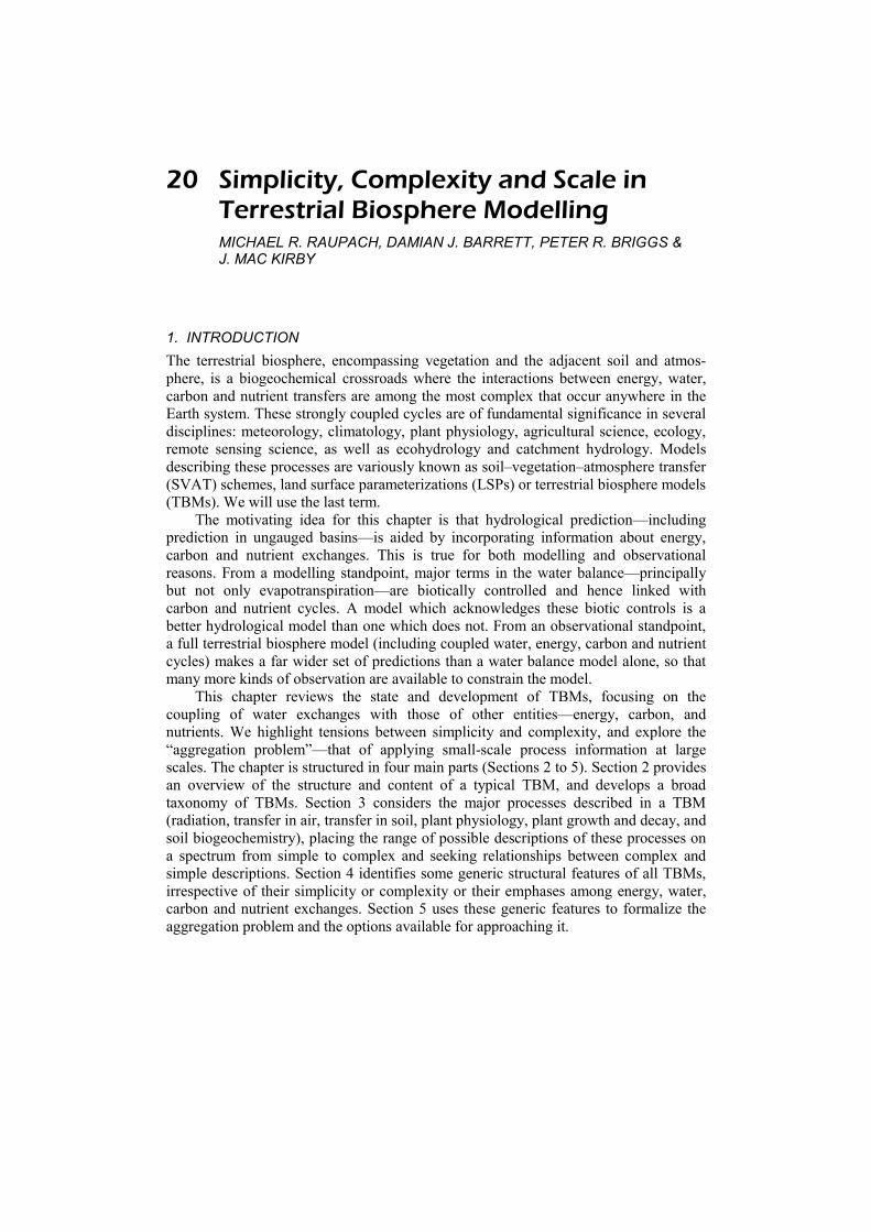
We note at the outset that there is a vast literature on TBMs, including hundreds of models developed over the last two decades. An early, seminal review of the underlying processes was the two-volume Vegetation and the Atmosphere edited by Monteith (1975, 1976). More recent reviews of process knowledge are provided by numerous chapters in books edited by Jarvis et al. (1989), Black et al. (1989), Bolle et al. (1993) and Kalma & Sivapalan (1995) (mainly from a hydrometeorological perspective), and Trenberth (1992) and Browning & Gurney (1999) (mainly from an atmospheric perspective). Kickert et al. (1999) have provided a recent model-oriented review from the perspective of predicting environmental and ecological change. Summaries of many existing TBMs are provided by two recent intercomparison programmes, the first being the Project for the Intercomparison of Land Surface Parameterization Schemes (PILPS: Henderson-Sellers et al. 1993, 1995; Chen et al. 1997; Timbal & Henderson-Sellers, 1998). It was found that 23 TBMs used in atmospheric models differ widely in their ability to reproduce measurements of energy and water fluxes, and that much of the difference is explainable through differences in the parameterization of soil hydrology and the water balance. A second major intercomparison, from the point of view of carbon exchange and Net Primary Productivity (NPP) at the global scale, was the Potsdam NPP Model Intercomparison (Cramer & Field, 1999; Cramer et al., 1999). Among 15 models of widely differing complexity and purpose, there was some spread but also significant broad agreement in predictions of both mean global terrestrial NPP (a range of 44.4 to 66.3 PgC year-1) and its large-scale spatial distribution. Again, sensitivity to the method of simulating the water balance was evident. 2. OVERVIEW OF TERRESTRIAL BIOSPHERE MODELS The main fluxes and stores of energy, water, carbon and nutrients in the terrestrial biosphere are indicated schematically in Fig. 20.1, together with some of the key process variables influencing them and some of the major pathways by which fluxes, stores and process variables are coupled. The task of a TBM is to describe the dynamics of this system and its responses to variations in weather, climate, land use and land management. Over the last three decades, a wide variety of TBMs has been developed for a wide range of ultimate applications as outlined in Section 1. Their common link is that they all describe the system sketched in Fig. 20.1, or some part of it. To map the range of approaches currently being employed, a taxonomy of TBMs can be developed using several criteria: (1) scope (range of biophysical processes); (2) scale (including both space and time, and distinguishing between domain and resolution); (3) application (intended use); and (4) complexity (in structure, number of state variables or number of parameters). To develop this taxonomy we first explore model scope, noting its associations with scale and application; complexity is treated later. Five classes of TBM can be identified:

Class 1 - Energy and water Many early TBMs considered only the fluxes and stores of water and energy, treating all other properties of the terrestrial biosphere as fixed. They were developed for applications in meteorology (to provide terrestrial lower boundary conditions for atmospheric models), hydrology (to estimate catchment water balances) and forestry, agriculture and irrigation science (to estimate plant

M. R. Raupach et al. Chapter 20, Terrestrial Biosphere Modelling 241

Fig. 20.1 Schematic representation of major stores, fluxes and process variables represented in a terrestrial biosphere model.

water requirements). Early models, and some successful current ones, were based on simple, robust biophysical concepts including the Penman-Monteith equation for the latent heat flux (e.g. Thom, 1975; Raupach, 2001), the 15 cm “Manabe bucket” for soil water (Manabe, 1969) or a simple “leaky bucket” representation of the soil water balance. Later TBMs in this class, including many of the models in the PILPS intercomparisons (Chen et al., 1997), use sophisticated treatments of radiation, turbulent exchanges and soil heat and water storage.

Class 2 - Energy, water and carbon It has long been understood that carbon and water exchanges are linked through plant stomatal conductance, but this linkage could only be utilized effectively in TBMs once the processes linking stomatal conductance and carbon assimilation were elucidated (Wong et al., 1979; Farquhar et al., 1980; Leuning, 1990, 1995; Collatz et al., 1991). It then became clear that inclusion of carbon exchanges in TBMs was important not only in its own right (because of the central role of carbon in the biosphere) but also because of the possibility of improved models of stomatal conductance and thence of plant canopy water fluxes. Early models in this class include those of Norman (1979), Norman & Polley (1989), and the pioneering Simple Biosphere (SiB) model (Sellers et al., 1986). Later work includes,


among others, the two-leaf model of Wang & Leuning (1998); several models of the coupling between the surface energy balance, vegetation physiology and the atmos-pheric boundary layer (Collatz et al., 1991; Baldocchi, 1992; Jacobs & de Bruin, 1992, 1997; de Bruin & Jacobs, 1993; Su et al., 1996; Raupach, 1998); and the hydrolog-ically-oriented WAVES model (Zhang et al., 1996, 1999a,b). Many of these models are now used to provide the terrestrial component in Global Climate Models (GCMs), for instance SiB (Xue et al., 1991) and the LSM model (Bonan, 1998).

Class 3 - Energy, water, carbon and nutrients Carbon exchange and stomatal conductance are often limited by nutrient availability, especially nitrogen and phosphorus. Schulze et al. (1994) argued that at the global scale and on time scales up to several years, N limitation is the primary control on global NPP. Nutrient levels in the terrestrial biosphere depend on nutrient cycling through the soil–plant system, including the uptake of nutrients into plants by growth, their release into the soil as litter, and the soil biogeochemical processes of nutrient mineralization and immobiliz-ation. In addition, nutrients are added to terrestrial pools by atmospheric wet and dry deposition, fixation (for N) and weathering (for P), and are removed by a variety of mechanisms including volatilization, leaching, sediment transport, fire, grazing and harvest. These processes are included in many TBMs aimed at understanding the role of the terrestrial biosphere in the global biogeochemical cycles of C, N and other entities. In some cases, nutrient limitation is included as an external control: examples include CASA (Potter et al., 1993, 1997), CARAIB (Warnant et al., 1994), PnET (Aber et al., 1995), and many of the other TBMs in the Potsdam NPP Model Intercomparison (Cramer & Field, 1999; Cramer et al., 1999). Other models include explicitly resolved nutrient cycles in plants, soil or both, notably the Century series of models (Parton et al., 1987, 1988, 1993) and the Introductory Carbon Balance Model (ICBM) family (Andrén & Kätterer, 1997; Kätterer & Andrén, 1999). These models are usually applied with time resolution from daily to annual because the processes of primary interest have long time scales (years to decades).

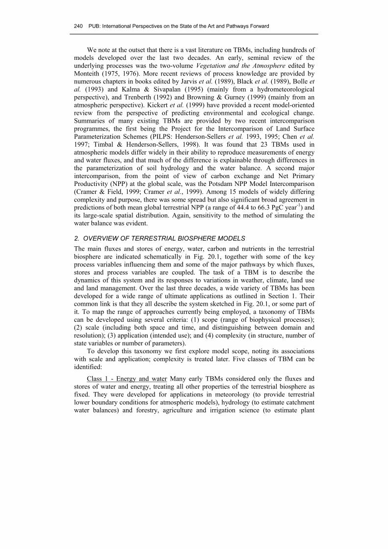
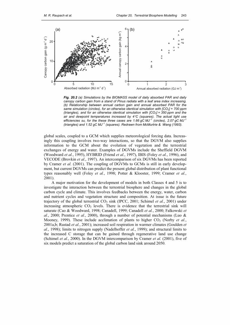
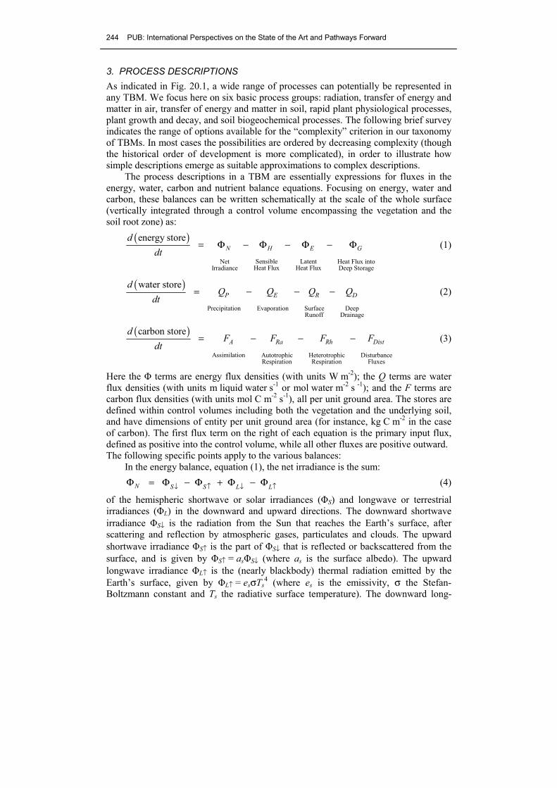
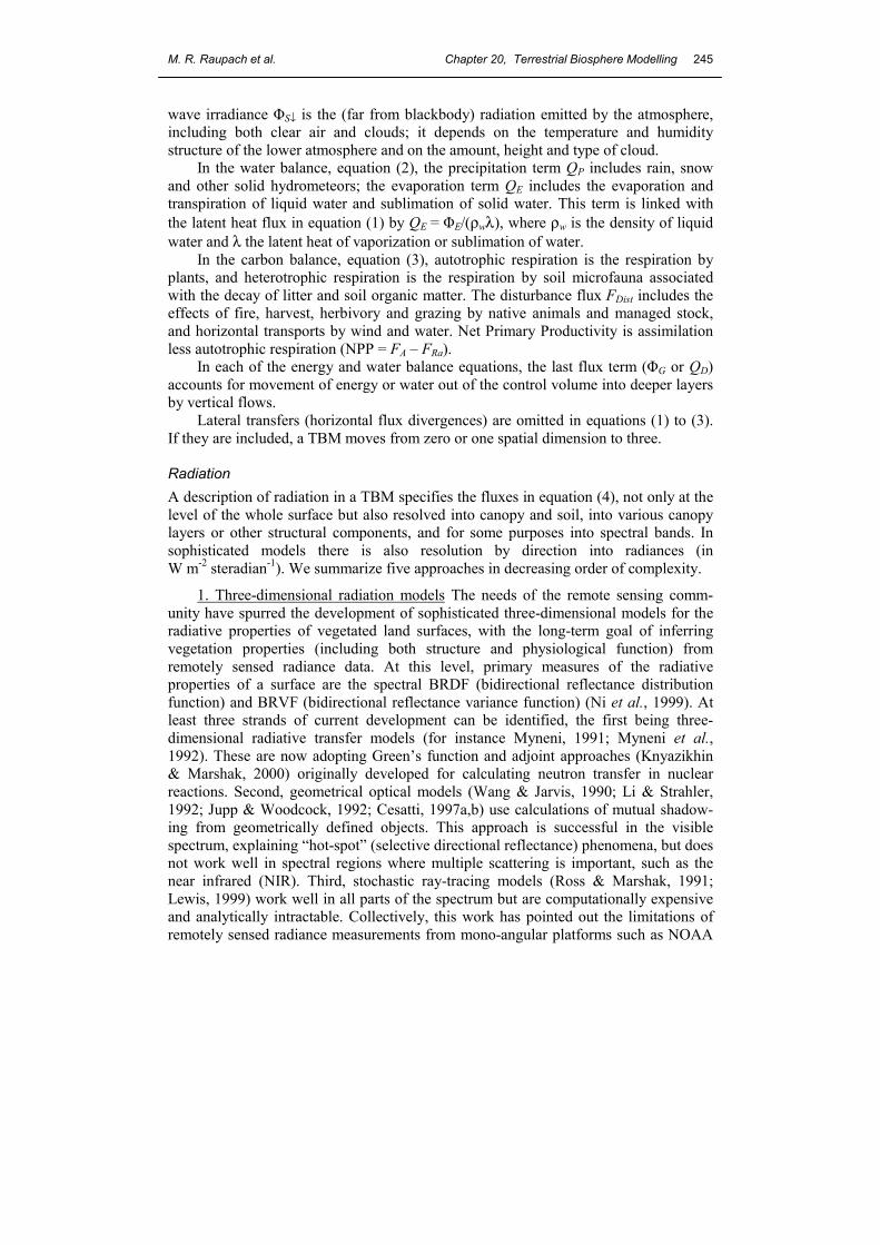
Class 4 - Energy, water, carbon and nutrients with plant dynamics For many applications concerned with plant management, a primary focus for a TBM is the growth and decay of plants and the associated pools of soil water, C, N and P. The TBMs serving these applications include crop pasture and forest growth models, often (but not always) highly parameterized for particular vegetation types. Examples include the forest growth models BIOMASS and G’DAY (McMurtrie et al., 1992; McMurtrie & Wang, 1993), 3PG (Landsberg & Waring, 1997) and CenW (Kirschbaum, 1999). Figure 19.2 illustrates the use of the BIOMASS model to predict annual growth increments of Pinus radiata, showing how temporal averaging smooths the relationship between assimilation and light interception.

Class 5 - Energy, water, carbon and nutrients with ecosystem dynamics At the global scale, plant dynamics are linked not only with land management as for the models in Class 4, but also with the evolution of terrestrial ecosystems. Models of this coupled system, known as Dynamic Global Vegetation Models (DGVMs), describe the stores and fluxes of carbon, water, and energy and their relation to the distribution and physiognomy of vegetation, and thence the physiological and structural responses of plant ecosystems to past or possible future climate change. Typically, they operate at


Fig. 20.2 (a) Simulations by the BIOMASS model of daily absorbed PAR and daily canopy carbon gain from a stand of Pinus radiata with a leaf area index increasing. (b) Relationship between annual carbon gain and annual absorbed PAR for the same simulation (circles), for an otherwise identical simulation with [CO2] = 700 ppm (triangles), and for an otherwise identical simulation with [CO2] = 350 ppm and the air and dewpoint temperatures increased by 4°C (squares). The actual light use efficiencies sεL for the these three cases are 1.66 gC MJ−1 (circles), 2.07 gC MJ−1 (triangles) and 1.52 gC MJ−1 (squares). Redrawn from McMurtrie & Wang (1993).

global scales, coupled to a GCM which supplies meteorological forcing data. Increas-ingly this coupling involves two-way interactions, so that the DGVM also supplies information to the GCM about the evolution of vegetation and the terrestrial exchanges of energy and water. Examples of DGVMs include the Sheffield DGVM (Woodward et al., 1995), HYBRID (Friend et al., 1997), IBIS (Foley et al., 1996), and VECODE (Brovkin et al., 1997). An intercomparison of six DGVMs has been reported by Cramer et al. (2001). The coupling of DGVMs to GCMs is still in early development, but current DGVMs can predict the present global distribution of plant functional types reasonably well (Foley et al., 1998; Potter & Klooster, 1999; Cramer et al., 2001). A major motivation for the development of models in both Classes 4 and 5 is to investigate the interaction between the terrestrial biosphere and changes in the global carbon cycle and climate. This involves feedbacks between the energy, water, carbon and nutrient cycles and vegetation structure and composition. At issue is the future trajectory of the global terrestrial CO2 sink (IPCC, 2001; Schimel et al., 2001) under increasing atmospheric CO2 levels. There is evidence that the terrestrial sink will saturate (Cao & Woodward, 1998; Canadell, 1999; Canadell et al., 2000; Falkowski et al., 2000; Prentice et al., 2000), through a number of potential mechanisms (Luo & Mooney, 1999). These include acclimation of plants to higher CO2 (Norby et al., 2001a,b; Rustad et al., 2001); increased soil respiration in warmer climates (Goulden et al., 1998); limits to nitrogen supply (Nadelhoffer et al., 1999); and structural limits to the increased C storage that can be gained through regenerative land use change (Schimel et al., 2000). In the DGVM intercomparison by Cramer et al. (2001), five of six models predict a saturation of the global carbon land sink around 2050.

10

20

0 0 5 10 15

Absorbed radiation (MJ m d )-2 -1

Can

opy

carb

on g

ain

(g m

d)

-2-1

a

00

2

6

4

1 2 3

Annu

al c

anop

y ca

rbon

gai

n (k

g m

)-2

Annual absorbed radiation (GJ m )-2

b(a) (b)


3. PROCESS DESCRIPTIONS As indicated in Fig. 20.1, a wide range of processes can potentially be represented in any TBM. We focus here on six basic process groups: radiation, transfer of energy and matter in air, transfer of energy and matter in soil, rapid plant physiological processes, plant growth and decay, and soil biogeochemical processes. The following brief survey indicates the range of options available for the “complexity” criterion in our taxonomy of TBMs. In most cases the possibilities are ordered by decreasing complexity (though the historical order of development is more complicated), in order to illustrate how simple descriptions emerge as suitable approximations to complex descriptions. The process descriptions in a TBM are essentially expressions for fluxes in the energy, water, carbon and nutrient balance equations. Focusing on energy, water and carbon, these balances can be written schematically at the scale of the whole surface (vertically integrated through a control volume encompassing the vegetation and the soil root zone) as:

( )

Sensible LatentNet Heat Flux intoHeat Flux Heat FluxIrradiance Deep Storage

energy storeN H E G

ddt

= Φ − Φ − Φ − Φ (1)

( )

Precipitation Evaporation Surface DeepRunoff Drainage

water storeP E R D

dQ Q Q Q

dt= − − − (2)

( )

Assimilation Autotrophic Heterotrophic DisturbanceRespiration Respiration Fluxes

carbon storeA Ra Rh Dist

dF F F F

dt= − − − (3)

Here the Φ terms are energy flux densities (with units W m-2); the Q terms are water flux densities (with units m liquid water s-1 or mol water m-2 s -1); and the F terms are carbon flux densities (with units mol C m-2 s-1), all per unit ground area. The stores are defined within control volumes including both the vegetation and the underlying soil, and have dimensions of entity per unit ground area (for instance, kg C m-2 in the case of carbon). The first flux term on the right of each equation is the primary input flux, defined as positive into the control volume, while all other fluxes are positive outward. The following specific points apply to the various balances: In the energy balance, equation (1), the net irradiance is the sum: N S S L L↓ ↑ ↓ ↑Φ = Φ − Φ + Φ − Φ (4)

of the hemispheric shortwave or solar irradiances (ΦS) and longwave or terrestrial irradiances (ΦL) in the downward and upward directions. The downward shortwave irradiance ΦS↓ is the radiation from the Sun that reaches the Earth’s surface, after scattering and reflection by atmospheric gases, particulates and clouds. The upward shortwave irradiance ΦS↑ is the part of ΦS↓ that is reflected or backscattered from the surface, and is given by ΦS↑ = asΦS↓ (where as is the surface albedo). The upward longwave irradiance ΦL↑ is the (nearly blackbody) thermal radiation emitted by the Earth’s surface, given by ΦL↑ = esσTs

4 (where es is the emissivity, σ the Stefan-Boltzmann constant and Ts the radiative surface temperature). The downward long-


wave irradiance ΦS↓ is the (far from blackbody) radiation emitted by the atmosphere, including both clear air and clouds; it depends on the temperature and humidity structure of the lower atmosphere and on the amount, height and type of cloud. In the water balance, equation (2), the precipitation term QP includes rain, snow and other solid hydrometeors; the evaporation term QE includes the evaporation and transpiration of liquid water and sublimation of solid water. This term is linked with the latent heat flux in equation (1) by QE = ΦE/(ρwλ), where ρw is the density of liquid water and λ the latent heat of vaporization or sublimation of water. In the carbon balance, equation (3), autotrophic respiration is the respiration by plants, and heterotrophic respiration is the respiration by soil microfauna associated with the decay of litter and soil organic matter. The disturbance flux FDist includes the effects of fire, harvest, herbivory and grazing by native animals and managed stock, and horizontal transports by wind and water. Net Primary Productivity is assimilation less autotrophic respiration (NPP = FA – FRa). In each of the energy and water balance equations, the last flux term (ΦG or QD) accounts for movement of energy or water out of the control volume into deeper layers by vertical flows. Lateral transfers (horizontal flux divergences) are omitted in equations (1) to (3). If they are included, a TBM moves from zero or one spatial dimension to three. Radiation A description of radiation in a TBM specifies the fluxes in equation (4), not only at the level of the whole surface but also resolved into canopy and soil, into various canopy layers or other structural components, and for some purposes into spectral bands. In sophisticated models there is also resolution by direction into radiances (in W m-2 steradian-1). We summarize five approaches in decreasing order of complexity.

1. Three-dimensional radiation models The needs of the remote sensing comm-unity have spurred the development of sophisticated three-dimensional models for the radiative properties of vegetated land surfaces, with the long-term goal of inferring vegetation properties (including both structure and physiological function) from remotely sensed radiance data. At this level, primary measures of the radiative properties of a surface are the spectral BRDF (bidirectional reflectance distribution function) and BRVF (bidirectional reflectance variance function) (Ni et al., 1999). At least three strands of current development can be identified, the first being three-dimensional radiative transfer models (for instance Myneni, 1991; Myneni et al., 1992). These are now adopting Green’s function and adjoint approaches (Knyazikhin & Marshak, 2000) originally developed for calculating neutron transfer in nuclear reactions. Second, geometrical optical models (Wang & Jarvis, 1990; Li & Strahler, 1992; Jupp & Woodcock, 1992; Cesatti, 1997a,b) use calculations of mutual shadow-ing from geometrically defined objects. This approach is successful in the visible spectrum, explaining “hot-spot” (selective directional reflectance) phenomena, but does not work well in spectral regions where multiple scattering is important, such as the near infrared (NIR). Third, stochastic ray-tracing models (Ross & Marshak, 1991; Lewis, 1999) work well in all parts of the spectrum but are computationally expensive and analytically intractable. Collectively, this work has pointed out the limitations of remotely sensed radiance measurements from mono-angular platforms such as NOAA


AVHRR, relative to newer multi-angular instruments such as MISR (Diner et al., 1989). The future of multi-angular remote sensing is reviewed by Liang et al., (2000). Because of their relatively high computational cost and the fact that they are designed mainly to describe radiances at the top of the canopy, three-dimensional radiation models have not been applied in TBMs to date. They do, however, constrain simpler radiation models and connect TBMs with remotely sensed information.

2. One-dimensional multi-layer radiation models A number of models have been developed, specifically for implementation in TBMs, to describe the one-dimensional (vertical) distribution of radiation (Norman, 1979; Sellers, 1985; Sellers et al., 1992; Goudriaan & van Laar, 1994). By integrating the three-dimensional radiation field over downfacing and upfacing hemispheres, these models provide analytic expressions for the downward and upward irradiances in broad spectral bands such as visible, NIR and thermal, separately resolving the direct and diffuse solar beams. The simplest such expression is Beer’s law for the down-flowing solar irradiance: ( ) ( ) ( )0 expS S c↓ ↓Φ ς = Φ − ς (5)

where ζ is the cumulative leaf area index downward from the top of the canopy (ζ = 0) and c is an extinction coefficient, typically around 0.6 but dependent on solar elevation and leaf angle distribution (Denmead, 1976).

3. Two-layer (canopy and soil) two-leaf models The idea behind these models originated with Sinclair et al. (1976) and Spitters (1986), but was implemented in TBMs only in the late 1990s (de Pury & Farquhar, 1997; Wang & Leuning, 1998; Wang, 2000; Choudhury, 2000). The principle is to integrate (over ζ) the sunlit and shaded portions of the canopy. This yields two idealized “big leaves” occupying the canopy layer of the model, the soil being an additional layer. Spectral resolution into visible, NIR and thermal bands is retained. This is likely to emerge as a good compromise which retains simplicity in model structure while capturing the essential nonlinear dependence of photosynthetic light use efficiency by leaves on their radiation environ-ment: shaded leaves use light more efficiently than sunlit leaves because they operate on different parts of nonlinear light response curves (Lambers et al., 1998; Nobel, 1999). A variant on this approach is a three-point integration across the light response curve (Calvet et al., 1998; Raupach, 1998). Models in this group are well adapted to link with mechanistic leaf-scale models of carbon and water exchanges (see below).

4. Two-layer (canopy and soil) single-leaf models These models carry integration yet further by treating only the canopy and the soil as radiatively distinct entities, each described by a direction-independent (solar) albedo, (thermal) emissivity and radiative surface temperature, lumping sunlit and shaded leaves together. This approach has been widely used in TBMs, especially those in Class 1 (energy and water); see for example Kowalczyk et al. (1991).

5. Bulk, whole-surface models An even stronger simplification is to combine vegetation and soil, using a single albedo, emissivity and radiative surface temperature for the whole surface. This level of simplification is usually excessive for a TBM, particularly if it is to describe sparsely vegetated surfaces. However, it offers an appropriate bulk description for highly integrative models of the Earth system.


Transfer of energy and matter in air Transfer of scalar entities (such as heat, water vapour, CO2 and other trace gases) through the air occurs through two consecutive pathways: the (usually) quasi-laminar boundary layers over individual surface elements such as leaves, and the turbulent air within and above the vegetation canopy or other roughness. We first consider transfer through the quasi-laminar element boundary layer. This is a very thin layer (typically less than 1 mm across) adjacent to the surface of a leaf or other surface element, in which the transfer of heat and matter is dominated by molecular diffusion rather than turbulent fluid motion because gradients in temperature and concentration are large and fluid velocities normal to the local surface are small. The qualifier “quasi” indicates that while fluid motion in this layer is usually laminar, it is also quite unsteady because of the highly turbulent nature of the flow in the canopy. Resistance to heat and mass transfer across quasi-laminar element boundary layers accounts for a significant portion of the total aerodynamic resistance, and therefore needs to be described. Fortunately simple formulations based on laminar boundary-layer theory are usually sufficient (for instance Thom, 1971, 1972; Monteith, 1973), though care is needed to account for several complications including the effects of mutual sheltering, unsteadiness, and turbulence in the canopy (Finnigan & Raupach, 1987). We turn now to the turbulent transfer through the air in the canopy. In the 1980s, it was recognized that coherent eddies play a dominant role in the transfer of energy, matter and momentum in the atmospheric boundary layer. In the air within and just above vegetation canopies, three broad scale ranges of eddy motion can be distinguished, respectively with length scales much larger than the canopy height hc, of the order of hc, and much smaller than hc. The large-size eddies (>>hc) are mainly responsible for horizontal turbulent motions in the canopy because of the constraining influence of the ground, and hence do not account directly for much vertical turbulent transfer. However, they modulate the growth, evolution and decay of smaller eddies. The middle-size eddies (of order hc) are responsible for most of the vertical motion and hence the vertical turbulent transfer of scalars. They are generated mainly by the strong shear (velocity gradient) near the top of the canopy. The small-size eddies (<<hc) are generated both by the decay of larger eddies and in the wakes of individual canopy elements such as leaves and stems. They are too small and not energetic enough to contribute much turbulent transfer, their main dynamical role being to dissipate energy from larger eddies and thence to heat. For a detailed account of this picture and the evidence which leads to it, see Raupach et al. (1996) and Finnigan (2000). In modelling these processes, four levels of complexity have emerged:

1. Large eddy simulation The most complete available description is provided by large-eddy simulation (LES), in which atmospheric momentum and scalar equations are solved numerically on a dense three-dimensional grid to resolve the full chaotic eddy structure (apart from small sub-grid-scale contributions) in both space and time (see for instance Moeng, 1984; Meneveau & Katz, 2000). LES techniques have recently been applied in vegetation canopies (Shaw & Schumann, 1992; Patton et al., 1998), using grids fine enough to resolve almost all the vertical transfer (that is, resolving all but the eddies with scales much smaller than hc in the above description). Like three-dimensional radiation models, LES is too numerically demanding to be suitable for routine use in TBMs. Its contributions are in parameterizing simpler


models, studying the feedbacks between surface processes and atmospheric turbulence at scales from canopy to region (Pielke et al., 1998; Avissar, 1998), and studying the dynamics of chemically active scalars where reaction times and eddy time scales are comparable (Patton et al., 2001).

2. Higher-order closure A different and older approach to modelling turbulent flow and scalar transfer is offered by higher-order closure, in which equations are constructed and solved for the means, variances and covariances of the momentum and scalar fields, resolved in space but averaged in time. This is a standard approach in fluid mechanics (Deardorff, 1973; Launder et al., 1975; Speziale, 1991). It was first applied to study the one-dimensional (vertical) structure of flows in vegetation canopies by Wilson & Shaw (1977) and has since been used in several model studies of the links between turbulent transfer and physiological activity, for instance by Meyers and Paw U (1986), Katul & Albertson (1998) and Pyles et al. (2000). The resulting models are Class 1 (energy, water) or Class 2 (energy, water, carbon) TBMs, currently used mainly for research purposes. Most higher-order closure models are too complex and parameter-intensive for large-scale application in Class 3, 4 or 5 TBMs.

3. Multi-layer non-diffusive or diffusive transport schemes A very old approach to studying the vertical transfer of scalars and momentum through the air layers in a canopy is based on the gradient-diffusion assumption:

( ) dCF z Kdz

= − ρ (6)

where F(z) is the vertical flux of a scalar (or momentum) at height z, C(z) is the scalar specific concentration or mass fraction (or the wind speed for momentum), ρ the air density and K(z) is a prescribed eddy diffusivity. This was the first approach used to construct multi-layer canopy models (for instance Cowan, 1968; Waggoner & Reifsnyder, 1968). However, the gradient-diffusion assumption does not hold in canopies, where countergradient fluxes can occur (Denmead & Bradley, 1987) because of the large length scales of the coherent eddies dominating in turbulent transfer in canopies (these scales are of the order of the canopy height hc, as indicated above). Several relatively simple theories have been developed to supply more physically realistic alternatives to the gradient-diffusion assumption, the first being “localized near-field” (LNF) theory (Raupach, 1989), which distinguishes diffusive “far field” and non-diffusive “near field” contributions to C(z). It has been applied in vegetation canopy models by Dolman & Wallace (1991), McNaughton & van den Hurk (1995), van den Hurk & McNaughton (1995), Katul et al. (1997), Leuning et al. (2000) and Leuning (2000). A second alternative is the “transilience” theory of Stull (1984, 1988), applied in vegetation canopies by Ni (1997). These non-diffusive theories are at an appropriate level for capturing the main physics of turbulent transport in TBMs when vertical resolution into multiple layers is required. A third, numerically demanding, approach is Lagrangian random-flight simulation (Thomson, 1987), applied in vegetation canopies by Baldocchi (1992) and Baldocchi & Harley (1995).

4. Two-layer (canopy and soil) or single-layer bulk transfer schemes These use variations of the generic formulation: ( )a s rF G C C= ρ − (7)


where F is the vertical surface-to-atmosphere scalar flux, Cs and Cr the concentrations at the surface and at a reference level in the atmospheric surface layer, and Ga the aerodynamic conductance (a bulk transfer coefficient with the dimension of velocity). This is the aerodynamic foundation of most bulk or single-layer models of land–atmosphere exchanges, including the Penman-Monteith evaporation equation and models for the dry deposition of trace gases and particles (Hicks et al., 1985). Equation (7) is a good model for aerodynamic transfer in TBMs that recognize only one vegetation layer, with a few provisos: first, the sequential resistances due to quasi-laminar elemental boundary layers and turbulent transfer need to be included in Ga. Second, the treatment of the element boundary-layer resistance needs to account for differences between momentum and scalar transfer arising from the bluff-body effect, the fact that momentum transfer or drag on a solid body in an airflow occurs at the surface through both pressure forces and molecular diffusion, but scalar transfer at the surface occurs through molecular diffusion alone (Thom, 1972). Third, evaluation of the turbulent-transfer part of Ga needs to account for the effect of thermal stability (the role of buoyancy) on turbulent transfer. Fourth, it is necessary to maintain the distinction between vegetation and soil surfaces, either by a “patch” approach in which vegetation and soil are separated horizontally (e.g. Kowalczyk et al., 1991), or by accounting for a soil layer beneath the vegetation (e.g. Raupach et al. 1997). Several workers (Shuttleworth & Wallace, 1985; van den Hurk & McNaughton, 1995; Blyth et al., 1999) have developed two-layer extensions of equation (7) in which a simple resistance network is used to combine vegetation and soil into a two-layer bulk transfer model compatible with a two-layer radiation model. Massman (1999) has included non-diffusive effects into such a formulation. Several simple models for momentum transfer in sparse canopies also account for the distinction between vegetation and soil by partitioning the drag between these two surface types, with implications for wind erosion and its suppression by vegetation (Shao, 2000). Transfer of energy and matter in soil The transfer of heat, water and solutes in the soil obeys well-known physical principles, heat transfer being governed by the diffusion or heat equation, and water transfer by Darcy’s law for soil water movement and Richards’ equation (Darcy’s law combined with conservation of mass). This might suggest that parameterization of these processes in a TBM is straightforward. However, complications arise from several sources: the nonlinearity of Richards’ equation, uptake of water and solutes by roots, and heterogeneity in both horizontal and vertical directions. Heat and water diffusion can be described using basic physical principles at several levels of complexity, leading alternatively to: (1) multi-layer, three-dimensional models, (2) multi-layer, one-dimensional models, (3) two-layer models, or (4) single-layer models. The principles underlying these methods are reviewed by Feddes et al. (1988), Philip (1988) and Gregory (1999). The basic parameters required are soil thermal and hydraulic properties, including heat capacity and diffusivity, water holding capacity and hydraulic conductivity (a strong function of soil water content). Many TBMs now use multi-layer, one-dimensional schemes for both soil heat and soil water (for instance Kowalczyk et al., 1991; Zhang et al., 1996; Verburg et al., 1997) in order to resolve soil heat and moisture fluxes with widely differing time scales (especially the daily and annual cycles), and to resolve water fluxes between soil and atmosphere


with strongly nonlinear dependencies on surface soil moisture (especially soil evaporation and infiltration). These schemes have largely replaced two-layer semi-analytic schemes such as the force-restore method of Deardorff (1977, 1978). Single-layer “leaky bucket” soil water schemes are also widely used, in which the leaks are functions of the soil water content in the bucket and represent outgoing water fluxes due to soil evaporation, drainage and plant water use. Uptake of water and solutes by roots is generally included through sink terms in each layer (Feddes et al., 1988, 1993). However, parameterizations for these terms require specification of rooting depths and sometimes the profile of root length density (Verburg et al., 1997). Major issues in describing the soil water balance arise from horizontal and vertical heterogeneity, including variability in soils, vegetation, topography and the distribution of precipitation. These issues become more important with increasing horizontal scale (both resolution and domain), but even at small horizontal scales the effects of topography and soil heterogeneity are of first-order significance (for instance Beven, 1995; Robinson & Sivapalan, 1995; Wood, 1995, 1999; Kim et al., 1997). There is currently intense debate about the treatment of soil and other forms of heterogeneity in the large-scale modelling of hydrological processes, around questions along the following lines: Can physical parameterizations at small scales be used at large scales, either without modification or with modified parameters (an example being the use of Darcy’s law at large scales with an “effective” hydraulic conductivity)? If small-scale parameterizations cannot be used or suitably adapted, how should they be replaced at large scales? How should large-scale parameter values be assigned, given the lack of information about soil heterogeneity in many cases? Does the inclusion of more small-scale physical processes improve model performance at large scales, especially in heterogeneous environments which are poorly measured? We consider generic approaches to some of these questions in Section 5. Plant physiological processes Plant physiological processes involve short-term exchanges of water, carbon and nutrients between plants and their environment, including photosynthetic carbon assimilation, autotrophic respiration, water uptake by roots and evaporation from leaves, and nutrient uptake. Descriptions of these processes fall into three strands.

1. Efficiency-based models For agricultural crops, Monteith (1977) and Kumar & Monteith (1981) introduced the idea of a maximum light use efficiency εL such that NPP = sεLΦPAR, where ΦPAR is the canopy-level flux of absorbed photosynthetically active radiation (PAR), and s is a stress function between 0 and 1 which accounts for limitations in resources other than light, primarily water and nutrients (see below). A theoretical, light-limited value for εL can be derived (Prince & Goward, 1995), but the actual efficiency (the product sεL, including light, water and nutrient limitations) is only a fraction of this value. The concept was extended to global scales by Field (1991) and Prince & Goward (1995), and now provides the basis for many global NPP models driven by remotely sensed data. It is intended for use at time intervals substantially longer than a day. Figure 19.2 shows (by the use of a more complex model) how the actual light use efficiency sεL becomes effectively constant under given external conditions as the averaging time increases.


An important aspect of light use efficiency is that it is strongly sensitive to the partition between direct and diffuse radiation (Jarvis et al., 1985; Hollinger et al., 1994). This may partly explain the increase in global plant assimilation in the early 1990s, through the effect of the Mt Pinatubo volcanic eruption (1992) in increasing the diffuse-to-direct radiation ratio (Roderick et al., 2001).

2. Stress-function models In this strand, key physiological parameters for a vegetated surface are the leaf stomatal conductance gs and the equivalent bulk surface conductance Gs for the entire canopy considered as a single big leaf, or for a few coarsely discretized canopy layers. Approximately, Gs is equal to the integral of gs over all canopy leaf surfaces (Kelliher et al., 1995). It was recognized early (e.g. Stewart & Thom, 1973) that gs and Gs vary in response to a number of environmental variables external to the plant. Jarvis (1976) proposed an empirical stress-function model to describe this variability, which at leaf scale is:

( ) ( ) ( ) ( )s sx PAR D s T s Wg g s s D s T s WΦ= Φ (8)

where gsx is a maximum conductance and the empirical functions s (between 0 and 1) account, respectively, for stresses resulting from low leaf-level absorbed PAR, ΦPAR, high leaf-surface saturation deficit Ds, high or low leaf temperature Ts, and low soil moisture W. An equivalent model can be written at canopy scale for Gs. This model is widely used (for instance Kowalczyk et al., 1991; Potter et al., 1993, 1997; Prince & Goward, 1995), though it is tending to be replaced by the more mechanistic models described next.

3. Mechanistic assimilation models Recently, more firmly grounded physiological models have emerged, based on the recognition that gs is closely coupled with photosynthetic carbon uptake (Wong et al., 1979; Farquhar et al., 1980; Ball et al., 1987). This approach considers three related physiological variables to be determined together (Leuning, 1990, 1995; Collatz et al., 1991): the leaf-level net carbon flux or assimilation rate fA (positive into a leaf), the intercellular CO2 concentration Ci, and gs itself. They are determined by three equations of the form:

( )

( )( )sD

s

As

issA

siA

DsCfg

CCgfTCf

=

−=φ= ,,func

(9)

where Cs, Ts and Ds (the leaf-surface CO2 concentration, temperature and deficit) are variables external to the leaf. The first of these equations is a biochemical model of the dependence of fA on Ci, the leaf PAR flux φ and leaf temperature Ts, of a form specified by Farquhar et al. (1980). The second equation is simply the definition of gs. The third is a statement about the control exerted on gs by humidity at the leaf surface, where the empirical function sD corresponds to that in equation (8). Ball et al. (1987) first proposed a form of this equation using relative humidity rather than the saturation deficit Ds, but Leuning (1995) provided empirical evidence that Ds is the better measure and that sD(Ds) = 1/(1 + Ds/D*), where D* is an empirical coefficient.


Models of this type represent a mechanistic link between the energy, water and carbon budgets, since the emerging value of gs can be used to determine the leaf evaporation, the leaf energy balance and the leaf temperature Ts from the Penman-Monteith and related equations (Raupach, 2001). Thus, a relationship is established between evaporation and carbon assimilation, through joint stomatal control. This approach was introduced into TBMs (within atmospheric models) by Collatz et al. (1991), Sellers et al. (1992, 1994) and Denning et al. (1996a,b). More recent research has focused on methods for scaling from leaf to canopy scale, in particular by combining a mechanistic assimilation model with the two-layer (canopy and soil) two-leaf radiation model described earlier in Section 3 (de Pury & Farquhar, 1997; Wang & Leuning, 1998). Plant growth and decay

The above models for assimilation rate FA or NPP assume fixed structural properties of the vegetation canopy, such as leaf area index, height and root distribution. However, the structure of the canopy alters in response to the combination of carbon assimilation, allocation of carbon by plants to their structural components (leaves, stems, roots), and plant death or litterfall. Some TBMs explicitly determine the changes in carbon stores in these components, by solving equations of the form:

( )jj A Ra j j

dCa F F k C

dt= − − (10)

where Cj is the carbon store in component j of the canopy; aj is an allocation ratio determining the fraction of net growth (NPP = FA − FRa) to component j (such that the sum of all aj is 1); and kj is a rate constant or inverse turnover time for the mortality of plant material. Equation (10) implies that at equilibrium, the stores, allocation ratios and rate constants are related by Cj = (aj/kj)NPP, which provides a useful constraint on the values of the parameters aj and kj (Barrett, 2002). The allocation ratios are often specified as simple functions of broad vegetation or biome type and moisture availability, for example as in Landsberg & Waring (1997) and most of the Class 3 (energy, water, carbon, nutrient) models for NPP described previously. However, recent developments are introducing more realism into descriptions of allocation. Many of these are based on the “resource balance” hypothesis (Field, 1983; Field et al., 1995) or the related “balanced activity” hypothesis (Davidson, 1969; Hilbert & Reynolds, 1991) that ecological processes tend to adjust plant characteristics in response to ambient conditions (resources available to the plant) in a way that tends to maximize growth. Thus, plants have adapted their allocation of carbon so that all acquired resources become equally limiting on average (Bloom et al., 1985), in order to maximize net benefit for growth and reproduction. This hypothesis is consistent with the fact that light, water and nutrient limitations, each considered separately, lead to similar values for the mean global terrestrial NPP. Recently, Friedlingstein et al. (1999) have explored the concept of dynamic determination of allocation ratios in a global-scale model. Enquist et al. (1999) used allometric scaling arguments to explain allocation over plant life histories.


Biogeochemical cycling Plants exchange carbon and nutrients with their soil environment in continuous biogeochemical cycles. The motivation for describing these cycles in a TBM is to account for the role of nutrients in modulating plant physiological activity and growth. The cycles are usually idealized by defining a set of control volumes and pools for carbon and nutrients, typically including plant (leaf, wood, root), litter (metabolic, structural/lignified), soil organic (active/microbial, slow/humic, passive/inert), and mineral nutrient pools (where slashes distinguish synonyms for functionally similar pools). Models for these processes rest on a common foundation (Jenkinson & Rayner, 1977; McGill et al., 1981; Parton et al., 1987) in which first-order rate equations are constructed for the carbon and nutrient pools. The flows of carbon between pools are determined by rate constants for microbial decay depending on temperature and moisture, with empirically determined fractional losses of carbon to soil respiration. The major nutrients (N, P and in some models S) flow with the carbon, with fluxes determined by prescribed ranges of C:N and C:P ratios for the destination pool for each transfer. Nutrient transfers between organic pools are accompanied by mineralization or immobilization (respectively, nutrient flow to or from the mineral nutrient pools). A comprehensive carbon and nutrient (N, P, S) cycling model based on this concept is Century (Parton et al., 1987, 1988, 1993), designed originally for grasslands. This model includes passive pools with very long time constants of hundreds of years. Another long-standing model is the Rothamsted soil carbon model (Jenkinson, 1990), in which the passive pool is not treated dynamically. The models CASA (Potter et al., 1993, 1997) and PnET (Aber et al., 1995, 1996, 1997; Aber & Driscoll, 1997) restrict nutrient considerations to nitrogen only. The ICBM models (Andrén & Kätterer, 1997; Kätterer & Andrén, 1999) use analytic solutions to simplified equations. The tension between complexity and simplicity To conclude this section, we note that the level of complexity in process descriptions involves a well-known trade-off: more complex (and therefore realistic) process descriptions involve more parameters. Models with few parameters cannot describe complex processes over a wide range of external (for instance climate) conditions, while models with many parameters cannot be constrained with available data (the problem of “equifinality”; Beven, 1995; Franks et al., 1997; Franks & Beven, 1999). Recent work on parameterization of TBMs (e.g. Raupach et al., 2005) applies “model-data fusion” techniques in order to combine data of several different kinds as multiple constraints for parameterization, thus reducing the equifinality problem. Data being used in this way include: (1) fluxes of water, carbon and other entities at long-term “FluxNet” sites (Olson et al., 1999; Law et al., 2000; Valentini et al., 2000; Baldocchi & Wilson, 2001); (2) atmospheric composition data on concentrations of CO2 and other gases (Kaminski et al. 2002; Wang & McGregor 2003); (3) in situ biomass and eco-logical measurements; (4) remote sensing of terrestrial surface properties; and (5) hydro-logical data (streamflow, soil moisture) as described elsewhere in this volume. In addition to the development of increasingly sophisticated parameterization methods, the complexity–simplicity tension is also driving model evolution, towards models with the most “skill per parameter”. As argued in the conclusion, this is resulting in the emergence of process descriptions of intermediate complexity.


4. GENERAL ATTRIBUTES OF TERRESTRIAL BIOSPHERE MODELS Structure The discussion so far suggests that all terrestrial biosphere models have many structural elements in common, in that they always represent the terrestrial balances of energy, water, carbon and nutrients, for a limited number of pools or stores defined by a set of control volumes (in the sense of regions of space) within which mass or energy balances can be constructed. Process descriptions of the kinds outlined in the previous section express the fluxes into and out of each pool in terms of the pool contents, forcing variables representing the weather and other external controls, and a few process parameters. The resulting mass or energy conservation equations are then solved at a resolution dependent on the application. The choice of pools and control volumes is critical, as it determines the spatial resolution of the model and also the level of process resolution. The horizontal boundaries of the control volumes define the landscape elements resolved by the model, which may be representative elementary areas (in hydrology), quasi-homogeneous patches (in meteorology or ecology) or pixels (in remote sensing). Within each landscape element, the pools and control volumes typically consist of a subset of the following: – Water stores: soil moisture in layers resolving at least the surface and deep root

zones, and often in multiple layers or compartments. – Energy stores: temperatures or thermal stores in layers similar to those for water. – Carbon stores: leaf, wood and root C pools in live vegetation, one or more litter C

pools, and active, humic and passive soil C pools (possibly resolving below-ground pools into soil layers).

– Nutrient stores: similar pools as for carbon, together with mineral pools in the soil. Practically all TBMs carry explicit water stores and most carry explicit energy stores. In the terminology of the second section, carbon stores are carried in TBMs of Classes 2, 3, 4 and 5, and nutrient stores in Classes 3, 4 and 5. The art of developing a TBM consists of: (1) choosing the pools, control volumes (hence spatial resolution) and time resolution to resolve the processes under study, without carrying unnecessary detail; (2) forming the mass or energy balance equations governing these pools; (3) forming expressions for the fluxes which are appropriate and robust at these space and time scales; (4) finding the parameters in the flux expressions; (5) solving the equations; and (6) comparing with data, which may involve parameter adjustment. To formalize the generic structure of a TBM, suppose that xr(t) is the energy or the mass of water, carbon or nutrient in store r at time t. As indicated by the examples of equations (1) to (3), the conservation equation governing xr is generically:

1 2r

r r rss

x f f ft

∂ = + + =∂ �� (11)

where frs is the flux or transformation which changes the content of store r by process s. Fluxes account for movement across the boundary of the control volume, for instance evaporation or deep drainage of water, or assimilation or respiration of carbon, whereas transformations account for conversions between stores within the control volume, such as the conversion of biomass to litter. All frs terms will henceforth be called fluxes. In general, these terms depend on three kinds of variable: (1) the state of the


system, specified by the store contents xr; (2) external forcing of the system, by meteorology (mainly through rainfall, solar radiation, temperature and humidity) or by land management (for instance the supply of additional resources through irrigation or fertilization); and (3) parameters such as light use efficiency or soil hydraulic properties. Using bold letters to denote sets of variables, the fluxes and transformations can then be written:

f = { frs }; frs = frs (x,m,p) (12)

where f, is the set of fluxes, x the set of stores, m the set of external forcing variables representing meteorological and land-management influences, and p the set of parameters. Equation (12) is a generic representation of the all the process descriptions in the previous section. The equations in this set are always empirical to some extent, even in the most mechanistic of models, and are analogous to the “phenomenological” equations used to describe fluxes in non-equilibrium thermodynamics (Prigogine, 1961; de Groot & Mazur, 1962). A TBM consists generically of the coupled system defined by equations (11) and (12), in which the unknowns are the sets of stores x and fluxes f, and the sets of forcing variables m and parameters p are prescribed. There is a fundamental difference between equations (11) and (12): equation (11) is a set of differential conservation equations governing the evolution of the store contents x(t) in time, while equation (12) is a set of algebraic phenomenological equations specifying the fluxes f. Together, equations (11) and (12) form a mathematically closed system in x and f. To achieve closure, each flux frs must be specified by a version of equation (12). The forcing variables m are strongly dependent on both time and space, reflecting the variability of weather and land management at space scales from local to global, and time scales from less than diurnal to multi-annual and beyond. The parameters p may also depend on space and time, in ways discussed shortly. The space-time dependencies of the solutions for the dependent variables (x and f) are entirely determined by those of the independent variables (m and p), with the equation system itself remaining the same over the whole space and time domain. The parameters p are of three kinds: process parameters, pprocess (such as light use efficiency or maximum photosynthetic capacity); properties of the soil or landform, psoil (such as soil depth or layer structure, and the hydraulic and thermal properties of soil layers); and properties of the vegetation, pveg (such as height, leaf area index or albedo). These have different characteristics: first, parameters in the set pprocess reflect basic properties of plant physiology, radiative transfer and atmospheric turbulence near the terrestrial surface. They are independent of both space and time, except possibly for a dependence on broad biome properties such as differences between C3 and C4 plant physiology, and are usually prescribed, at least initially, from basic theory or process experimentation. Second, soil and landform properties psoil are strongly dependent on space at all scales, reflecting the heterogeneity of natural and managed landscapes. They are usually regarded as time-independent, although some time dependence can arise mainly through land management. They are often specified from maps of soil and landform distribution in which land units are described by discrete attributes such as soil classes, after which look-up tables or pedotransfer functions can be used to relate soil physical and chemical properties to the mapped classes. Third, vegetation properties pveg depend on both space and time through the spatial and temporal


distribution of vegetation. They can be specified from maps of vegetation distribution based on a discrete vegetation classification such as biome types, from which the necessary properties are inferred using lookup tables. In TBMs of Classes 4 and 5, some or all of these vegetation properties are internal dynamic variables determined as part of the system of equations (11) and (12). An example is leaf area index, which may be specified in terms of a leaf carbon store as one of the stores xr. Dynamic and steady-state models Equations (11) and (12) form a coupled set of differential and algebraic equations which together specify the evolution or time history of the stores x and the fluxes f in response to specified m and p. Determination of the unknowns x and f involves solving a set of differential equations in time, to find the dynamic or temporally evolving behaviour of the system. However, it is often sufficient to solve a much simpler problem, that of finding the steady or equilibrium state of the system. The steady-state solution arises when the storage changes ∂xr/∂t in equation (11) are much less than the fluxes, so that equation (11) reduces to fr1 + fr2 + … = 0. Equations (11) and (12) then become: ( ), , 0rs

sf =� x m p (13)

so the model reduces to a set of algebraic equations, a far easier proposition to solve. The steady-state solution is of great practical importance, for both mathematical and physical reasons. A first (though rather unrealistic) application is the “deterministic steady state”, that is, when the forcing variables m are constant in time. In this case, equation (13) yields the long-time limit of the stores x and thence the fluxes f for any initial store values x(0) at time t = 0. When m is constant (or can be assumed so), the time-dependent solution of equations (11) and (12) relaxes after a sufficient time to the time-independent solution of equation (13). Formally, this is true only when the steady-state solution satisfies dynamical stability conditions (Drazin, 1992; Beck & Schloegl, 1993), but these conditions are always met in practice in TBMs. A second, much more realistic application of the steady-state concept can be made in conditions where x, f, m and p are statistically stationary rather than strictly constant in time. This is a “statistical steady state”. Time averaging (by integration of equation (11) over a time period T) gives:

( ) ( )

0 0

01 1 orT T

r rrrs rs

s s

x T xx dt f dt FT t T T

� � −∂ = =� �∂ � �� (14)

where an upper case letter (F) denotes a time average over the period T. Suppose that the stores x(t) are statistically stationary over this period; that is, they have no statistical trends, although they may have random fluctuations from temporal variability in m and p. The term [xr(T)−xr(0)]/T then approaches zero as T increases, so that: 0 asrs

sF T→ → ∞� (15)

Provided also that the time-averaged fluxes Frs can be related to time-averaged stores X, forcing variables M and parameters P, the time-averaged model becomes

( ), , 0rss

F =� X M P , identical with equation (13) except that all variables are time-


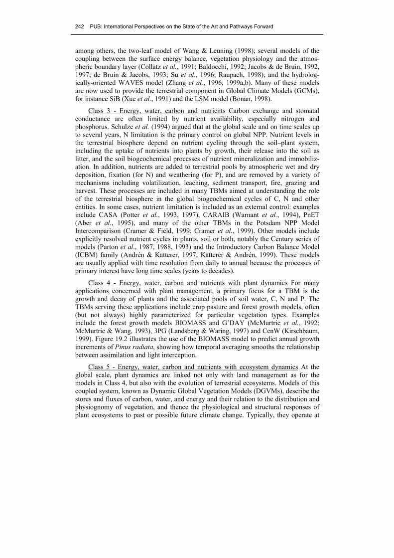
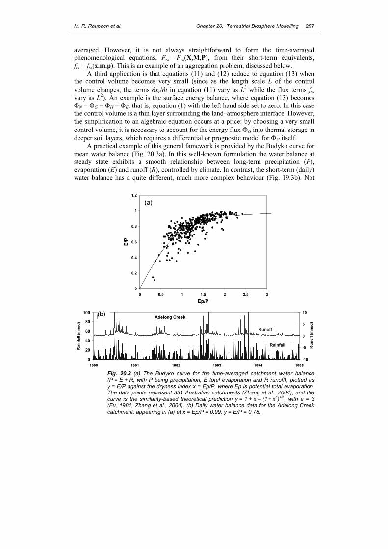
averaged. However, it is not always straightforward to form the time-averaged phenomenological equations, Frs = Frs(X,M,P), from their short-term equivalents, frs = frs(x,m,p). This is an example of an aggregation problem, discussed below. A third application is that equations (11) and (12) reduce to equation (13) when the control volume becomes very small (since as the length scale L of the control volume changes, the terms ∂xr/∂t in equation (11) vary as L3 while the flux terms frs vary as L2). An example is the surface energy balance, where equation (13) becomes ΦN − ΦG = ΦH + ΦE, that is, equation (1) with the left hand side set to zero. In this case the control volume is a thin layer surrounding the land–atmosphere interface. However, the simplification to an algebraic equation occurs at a price: by choosing a very small control volume, it is necessary to account for the energy flux ΦG into thermal storage in deeper soil layers, which requires a differential or prognostic model for ΦG itself. A practical example of this general famework is provided by the Budyko curve for mean water balance (Fig. 20.3a). In this well-known formulation the water balance at steady state exhibits a smooth relationship between long-term precipitation (P), evaporation (E) and runoff (R), controlled by climate. In contrast, the short-term (daily) water balance has a quite different, much more complex behaviour (Fig. 19.3b). Not

Fig. 20.3 (a) The Budyko curve for the time-averaged catchment water balance (P = E + R, with P being precipitation, E total evaporation and R runoff), plotted as y = E/P against the dryness index x = Ep/P, where Ep is potential total evaporation. The data points represent 331 Australian catchments (Zhang et al., 2004), and the curve is the similarity-based theoretical prediction y = 1 + x – (1 + xa)1/a, with a = 3 (Fu, 1981, Zhang et al., 2004). (b) Daily water balance data for the Adelong Creek catchment, appearing in (a) at x = Ep/P = 0.99, y = E/P = 0.78.

0

0.2

0.4

0.6

0.8

1

1.2

0 0.5 1 1.5 2 2.5 3Ep/P

E/P

a

0

20

40

60

80

100

1990 1991 1992 1993 1994 1995

Rai

nfal

l (m

m/d

)

-10

-5

0

5

10R

unof

f (m

m/d

)

Runoff

Rainfall

Adelong Creekb

(a)

(b)


only are storage changes important at short time scales, but also the phenomenological equations used to describe fluxes at the two different time scales are quite different: a simple similarity-based theory works well for the steady-state (Fu, 1981; Zhang et al., 2004) but not at short time scales where storage changes and threshold phenomena are important. 5. AGGREGATION AND DISAGGREGATION

Motivations TBMs and their constituent process descriptions are always specific to particular space and time scales, through the assumed phenomenological equations (12). For example, canopy-scale models describe stores and fluxes in a spatially homogeneous vegetation canopy. Related, but not identical, models can also be developed at the (smaller) leaf scale, exemplified by many of the more complex process descriptions in Section 3 and at the (larger) landscape scale, to describe the behaviour of spatially averaged stores and fluxes across an extensive, heterogeneous area. Similarly, models at subdiurnal, diurnal and longer time scales often have different forms. It is often necessary to apply information at one scale to a different (smaller or larger) scale in space or time. The transfer of information from smaller to larger scales is known as upscaling or aggregation, while conversely, downscaling or disaggregation is the transfer of information from larger to smaller scales. In general we will denote the small-scale or finely-resolved variables (in space or time) by lower case letters (x, f, m, p), and the large-scale, coarsely-resolved, space or time averaged variables by upper case letters (X, F, M, P). The information to be transferred across scales may include forcing variables (m ↔ M), model parameters (p ↔ P) or process descriptions encapsulated in the functional forms of the phenomenological equations [f(x,m,p) ↔ F(X,M,P)]. Common examples of aggregation problems include estimation of surface runoff from catchments using point hydrological models, calculations of lake nutrient loading from stream-based models, estimation of plant canopy net photosynthesis from leaf-scale models, prediction of terrestrial carbon sources and sinks for national greenhouse gas inventories from point-based models, and the specification of grid-cell averages of land-surface energy and water fluxes in large-scale atmospheric models (all problems in spatial aggregation); and the estimation of long-term water balances from time series or statistical information about rainfall and other forcing variables (a temporal aggregation problem). A common disaggregation problem is the specification of the spatial distribution of land-surface fluxes and meteorological variables, especially rainfall, from information available only in large-scale average form. These and similar problems have been a prominent research topic for over a decade, and have been the subject of major workshops in several disciplines: for instance Bolle et al. (1993) and Michaud & Shuttleworth (1997) primarily addressing meteorological problems, Ehleringer & Field (1993) for plant physiological problems, and Kalma & Sivapalan (1995) mainly for hydrological problems. Here we have little to say about disaggregation, except to note that it is primarily a statistical problem. It often involves the generation of finely resolved spatial fields or time series which have distributions consistent with known large-scale information, such as the means, variances and distribution functions of temperature or rainfall (Bates et al., 1998; Charles et al., 1999) or the correlation between rainfall and


topography (Hutchinson, 1995; Guenni & Hutchinson, 1998). Henceforth, this discussion concerns aggregation. Aggregated and disaggregated models The problem is to model the behaviour of the averaged stores and fluxes:

( ) ( ) ( ) ( )1 1

,N N

r r rs rsk k

X a k x k F a k f k= =

= =� � (16)

where the index k runs over a set of N points with weights a(k). This set might consist of the various kinds of land surface within an averaging area, with a(k) being the area fraction of land surface type k (an example of spatial averaging); or it might consist of points in time through a period T, with a(k) = ∆t/T for all k (an example of temporal averaging). There are two ways to approach this aggregation problem: by forming an aggregated model, or by using a distributed set of disaggregated models. In the aggregated-model approach, it is assumed that the average stores and fluxes obey a set of equations similar to the small-scale equations (11) and (12):

rrs

s

X Ft

∂=

∂ � (17)

( ), ,rs rsF F= X M P (18)

The aggregated conservation equations (equation (17)) follow directly from their small-scale counterparts (equation (11)) because of the linearity of the conservation equations and the superposition principle. Ways of obtaining the large-scale phenomenological equations, equation (18), are considered below. This approach is very widely used, being implicit in many canopy-scale TBMs. In the second (distributed) approach, the small-scale phenomenological equation (12) is evaluated N times, once for each point in the heterogeneous set, to produce a set of N fine-scale fluxes frs(k) which can be averaged using equation (16). This approach is conceptually direct and avoids the problem of forming a set of large-scale phenomenological equations, but it is often impractical, either because of its very high requirements for information (since m and p must be specified separately for each element k) or because of computational demand (since the number of distinct elements N may be very large). The distributed approach is very important and is also widely used, particularly in scaling from canopy to landscape. In GCMs, variability in land surface conditions within a grid cell is often represented by carrying several “tiles” or “patches” for each grid cell to represent the major land surface types (for instance Koster & Suarez, 1992). A “fuzzy disaggregation” approach has been introduced by Franks & Beven (1999) and Schulz et al. (2001) to simultaneously address the issues of the number of elements into which to disaggregate, and the uncertainties of the parameters in individual elements. It is often desirable to mix the aggregated-model and distributed-model approaches by using a distributed-model approach to represent the major sources of variability in the fine-scale f, x, m and p, and treating the residual variability with an aggregated model. The two-leaf (sun, shade) and two-layer (canopy, soil) models discussed in Section 3 are examples.


Aggregated phenomenological equations

Focusing on the aggregated model approach, let us consider ways of obtaining the aggregated phenomenological equations. Again there are two choices: either to assume that the functional form of the aggregated equations (18) is the same as that for the small-scale equations (12), or to seek a new, different functional form at the large scale. The latter option involves developing an entirely new relationship between Frs and the large-scale X, M and P; an example is the steady-state water balance equation for evaporation (Fu, 1981; Zhang et al., 2004) shown in Fig. 20.3. The former option is attractive because it represents an application of small-scale process information at the large scale through the assumption that the form of the function Frs and frs (in equations (18) and (12), respectively) are the same. However, a problem arises when the large-scale X, M and P are used to predict the aggregated Frs without considering the combined effects of model nonlinearity and variability in x, m and p at small scales. The problem occurs because in general:

( ) ( ) ( ) ( ) ( )( )1

, , , ,N

rs rsk

f a k f k k k=

≠ �X M P x m p (19)

unless the functional dependence of frs on x, m and p is linear (McNaughton, 1994). Strongly nonlinear phenomenological equations are common, for instance the Darcy law for soil water movement, threshold-based runoff (both infiltration-excess and saturation-excess), and the photosynthesis model underlying equation (9). This nonlinearity introduces a bias into the large-scale estimate of the fluxes, equal to the difference between the left and right hand sides of equation (19). Here are a few examples of bias in an aggregated model. The first (involving aggregation in time) is the estimation of average leaf photosynthesis from average irradiance on hourly time steps, using a nonlinear model of instantaneous leaf photosynthesis (Farquhar et al., 1980). Aggregation from fine time resolution to hourly time steps leads to an overestimation of photosynthesis by around 20% (Smolander & Lappi, 1985) because of the nonlinearity in the photosynthesis model. A second example is the highly nonlinear responses of soil organic matter decomposition to variations in temperature, as used in the Rothamsted (Jenkinson, 1990) or Century (Parton et al., 1988) models of soil organic matter dynamics. These produce erroneous estimates of soil C efflux when aggregated over long time periods (weeks to months) if the time-averaged value of soil temperature is used to estimate microbial respiration. Third, Beven (1995) studied the effect of random parameter distributions on evapo-transpiration as predicted by a hydrological model, demonstrating that variability in certain parameters (notably water holding capacity) leads to large model bias. Fourth, Raupach & Finnigan (1995) examined the effect of nonlinearity on aggregation over different land surface patches in a coupled model of the surface energy balance and the atmospheric convective boundary layer, showing that in this case the bias from model nonlinearity is relatively small because the nonlinearity is weak. Statistical estimation of bias

We now focus on the option of assuming that the aggregated and small-scale phenomenological equations have the same functional form. Yet again there are choices for how to proceed. One is to modify the parameters in the large-scale equation


to remove the bias, for instance by defining an “effective” hydraulic conductivity to describe water movement at large scales with a version of Darcy’s law. Beven (1995) called this the effective parameter approach, and criticized it on the grounds that the required values of the effective parameters are not unique, suffering from “equifinality” (Franks & Beven, 1997, 1999; Schulz et al., 2001). A second choice, which may be called “statistical estimation”, is to introduce statistical information on the variability of x, m and p which interacts with nonlinearity to produce the bias. The following analysis describes this approach. Let the combined set of variables x, m and p be denoted by v, so that v = {x,m,p} = {x1, x2,…, m1, m2,…, p1, p2,…}, and let prob(v) be the joint probability density function of all these variables. The distribution of p reflects small-scale variability in parameters; the distribution of m reflects stochastic variability in forcing; and the distribution of x reflects the system responses to both of the above kinds of variability. The phenomenological equations for the average fluxes then become:

( ) ( )probrs rsF f d= � v v v (20)

where the integral extends over the space of all values of v = {x,m,p}. Using a Taylor expansion of frs up to second order about the averaged state V = {X,M,P}, we obtain:

( ) ( )2

1 1 1... prob

2!

M M M i jrs rsrs rs i

i i ji i j

v vf fF f v dv v v= = =

� �′ ′∂ ∂′� �= + + +∂ ∂ ∂� �

� �� v v v (21)

where M is the number of elements in v, vi is element i of v, vi' denotes vi − Vi, and all partial derivatives are evaluated at the averaged state V. Evaluating the integrals over prob(v)dv as moments, we obtain

( )2 2 2

21 1 1

...2!

M M Mi rs rs

rs rs i j iji i j i i ji

f fF fv vv= = = +

σ ∂ ∂= + + σ σ ρ +

∂ ∂∂� � �V (22)

where σi is the standard deviation of vi and ρij is the correlation coefficient between vi and vj. The coarse-scale flux Frs is the sum of three terms: the fine-scale function frs(V) evaluated at the average values V = {X,M,P} of the stores, driver variables and parameters, and two terms, respectively, proportional to the variances and covariances of X, M and P. The bias in the aggregated model, Frs − frs(V), is given by these second and third terms. Each is the product of a second-order partial derivative of frs(v) which characterizes the extent of the nonlinearity in frs(v), and a variance or covariance of v which characterizes the variability in the stores, drivers and parameters. It is important to note that equation (22) is an approximation based on a Taylor expansion truncated at second order. The neglected higher-order terms, consisting of products of third and higher moments of v and third and higher derivatives of frs(v), may become significant if the distribution prob(v) is highly non-Gaussian or if the model is highly nonlinear. Simplification of equation (22) occurs in several circumstances. First, when frs(v) is linear, the bias (second and third) terms disappear because the second-order partial derivatives are zero. For linear models of independent variables and parameters, the estimated flux at the large scale is simply Frs = frs(V) evaluated at the mean values of the stores, driver variables and parameters. Second, when the variability (variances and covariances) of x, m and p are sufficiently small, the bias terms are also small. Conversely, when the combination of variability and model nonlinearity (second


derivatives in frs(v)) is large, the bias terms are also likely to be large. A third possible simplification is that when the elements of x, m and p are independent (ρij = 0), the third term in equation (22) disappears. Alternatively, positive and negative correlations may shift the bias away from zero in opposite directions, thereby cancelling. Equation (22) recasts the aggregation problem as a problem in statistical estimation, in which the main challenge is to estimate accurately the means, variances and covariances of model variables and parameters. This view has two significant implications: first, attempts to improve the performance of an aggregated model by further measurement of only the mean variables and parameters are futile, because measurements of mean quantities cannot eliminate bias arising from the interaction between model nonlinearity and small-scale variability. Improvement can only be obtained by quantifying this variability and its consequences for model bias through equation (22). Second, equation (22) can be used even if there is substantial uncertainty about the distribution prob(v) in equation (20), and hence the means, variances and covariances of the variables v. In these circumstances, even rough estimates of the means, variances and covariances will yield useful information about the bias in aggregated values of Frs when the model is highly nonlinear. Parameter estimation and scaling Parameters themselves are usually not directly observable, especially at large scales. Rather, they express the effects of processes outside the time or space scale of interest which cannot be treated explicitly in the phenomenological equations determining the fluxes. One technique for determining parameters is that of model inversion, that is, seeking the parameter values which optimize the fit of the model to simultaneous direct observations of both input and output variables. (Other techniques include application of a priori constraints and guessing). Model inversion is becoming increasingly sophisticated, including including use of model adjoints, gradient-based search methods, genetic algorithms and use of the Kalman filter. Recent examples include the combined use of atmospheric concentrations and remote sensing data to constrain parameters in a TBM for predicting carbon exchanges at large scales (Wang & Barrett, 2003; Wang & McGregor, 2003); use of atmospheric composition and eddy flux data at global scales to constrain a carbon-oriented TBM (Rayner et al., 2001); estimation of statistical parameters in a carbon cycle model (Barrett et al., 2001); use of genetic algorithms to constrain a carbon cycle model with ecological data (Barrett, 2002); and constraining parameters in a canopy-scale TBM from flux, concentration and isotope data (Styles et al., 2002) and model-data fusion with multiple constraints (Raupach et al., 2005). Care is required when aggregating small-scale parameters for use in large-scale phenomenological equations like equation (18). Parameters at small scales (p) are often identifiable with observable features of the system. However, two difficulties often arise when seeking aggregated parameters at large scales (P): the interpretation of a parameter may change as it assumes the statistical properties of a population rather than any individual element (k in equation (16)), and the distribution of the parameter through the population may be unknown. Two broad strategies for handling these problems are either to introduce additional small-scale information, or introduce “lumped” parameters at the large scale. The first alternative involves expressing unknown parameters as functions of variables which are already well known (either deterministically or statistically) at


small scales. This amounts to introducing new phenomenological information, or extending the phenomenological equations (12). Suppose that a certain parameter, say p1, has an unknown distribution at small scales. It may be possible to replace p1 with a known or estimated function of stores, driver variables and other parameters for which the distribution at small scales is known:

p1 = g(x, m, p2, p3, …) (23)

where the function g contains the additional information necessary to estimate p1 over all points in variable space. Thus, p1 ceases to be an externally prescribed parameter and becomes an additional unknown in the system of equations, with equation (23) providing the additional constraint necessary to close the system of equations with unknowns {x, f, p1}. An estimate of the bias in the large-scale parameter P1 can be obtained from the known variability of x, m and the other p (excluding p1) using an equation analogous to (22). Alternatively, equation (23) can be used to eliminate p1 completely from the phenomenological equations in favour of other variables with known distributions. A well studied example concerns the estimation of net canopy photosynthesis by light absorption using the canopy-scale (aggregated) parameter Jmax, the maximum photosynthetic capacity of the canopy (Harley & Baldocchi, 1995; de Pury & Farquhar, 1997; Wang & Leuning, 1998). The value of Jmax is calculated from the distribution of the equivalent leaf-scale (disaggregated) parameter jmax through the canopy, but this distribution is poorly known. However, additional information is available: a priori empirical evidence indicates jmax varies linearly as a function of leaf nitrogen concentration ([N]leaf) and that [N]leaf decreases approximately exponentially with increasing cumulative leaf area index downward from the top of the canopy. A theoretical basis for these observations lies with the hypothesis of optimal allocation of resources for photosynthesis, which implies that leaves receiving higher than average irradiance are allocated more nitrogen, and therefore have higher [N]leaf and higher jmax (Field, 1983; Field et al., 1995; Sands, 1995). By expressing jmax as a function of [N]leaf and introducing statistical information about the distribution of [N]leaf through the canopy, it is possible to integrate over leaf area index to obtain an averaged value of the parameter Jmax for canopy layers or for sun and shade leaf classes. In this example, the conceptual meaning of the parameters jmax and Jmax differ as the scale changes from leaf to canopy. The former parameter describes the biochemical and physical limitations of electron transport in the chloroplast membranes of leaf cells and can be accurately measured at the leaf scale. The latter is a weighted average of the former for all leaves of the canopy, that is, over a highly variable population. The variability in this population increases as the population extends over more and more scales (for instance, progressively thicker or coarser canopy layers). Because of the interaction between variability and model nonlinearity demonstrated by equation (23), the value of the aggregated parameter Jmax changes as the scale of integration increases. The second alternative is to introduce lumped or intrinsically large-scale parameters, which are not explicitly related to any small-scale process representations (for instance McKane et al., 1997). The introduction of lumped parameters is often (though not always) associated with alteration in the functional form of the phenomenological equations in the translation from small to large scales, that is, from equation (12) to (18). Model bias cannot be estimated with equation (22), and in fact


the concept of model bias used here loses meaning because the large-scale model is not based on a small-scale model and knowledge of its associated parameters, but rather on evidence applicable at the large scale only. 6. CONCLUDING SUMMARY This review of Terrestrial biosphere models (TBMs) has concentrated on four themes. First, in Section 2, we have attempted to classify TBMs developed for a wide range of different applications with a corresponding range of emphases and levels of sophistication. However, all describe aspects of the same system. Four criteria have been identified: scope or range of biophysical processes; space and time scale; application; and complexity. In terms of scope, five broad classes of TBM can be distinguished: Class 1: energy and water; Class 2: energy, water and carbon; Class 3: energy, water, carbon and nutrients; Class 4: energy, water, carbon and nutrients with plant dynamics; and Class 5: energy, water, carbon and nutrients with ecosystem dynamics. These classes serve different broad applications, with different emphases in space and time scales, but all involve a core set of common processes. The second theme (Section 3) is an exploration of process representations, or the “complexity” criterion. Six major groups of process are considered: radiation, transfer of energy and matter in air, transfer of energy and matter in soil, plant physiological processes, plant growth and decay, and soil biogeochemical processes. In each case, a variety of levels of description is available, ranging from very simple to very complex: for example, radiation can be described in several ways ranging from three-dimensional models to bulk, whole-surface models, and turbulent transfer in ways ranging from large-eddy simulation to single-layer bulk transfer schemes. This survey suggests three generalizations: First, the historical development of the most simple and most complex descriptions was initially largely independent, with a subsequent gradual convergence as simple descriptions were later formulated as rational approximations to more complex ones. Second, from a practical viewpoint, the most complex available descriptions are too cumbersome numerically and too demanding of parameters to be applicable in TBMs (except for the purpose of research into the relevant processes) while the most simple descriptions have insufficient capability to resolve important process components of the terrestrial biosphere (such as the distinction between soil and vegetation fluxes). Third, both these factors have spurred the development of descriptions of intermediate complexity, in which necessary process distinctions are maintained but judicious averaging (in space and time or over processes) is used to obtain relatively simple descriptions. Examples are two-layer (canopy and soil) two-leaf models for radiation, heat and mass transfer, and the convergence between efficiency-based models and mechanistic assimilation models for carbon uptake. Because of their blend of insight and computability, intermediate-complexity descrip-tions are becoming widespread throughout the classes of scope and application surveyed in Section 2. The third theme, treated in Section 4, is that all TBMs have generic structural features in common, irrespective of their simplicity or complexity or their emphases among energy, water, carbon and nutrient exchanges. They always involve the terrestrial balances of energy, water, carbon (for Class 2 and above) and nutrients (for Class 3 and above) for a limited number of pools or stores defined by a set of control volumes within which mass or energy balances can be constructed. This system is


described by two underlying generic sets of equations: a set of conservation equations expressing changes in pool contents (x) in terms of fluxes (f) into and out of the pools, and a set of phenomenological equations of the form f = f(x,m,p) describing the fluxes in terms of pool contents, forcing variables m and parameters p (with bold letters denoting sets of variables). By identifying this structure, it is possible to distinguish the different roles and properties of conservation equations (differential equations describing changes in store contents x, linear in both x and f) and phenomenological equations (algebraic equations for the fluxes f, often nonlinear). It is also possible to distinguish between dynamic TBMs, involving the solution of differential equations, and steady-state TBMs involving only algebraic equations of the form 0rs

sf =�

(where r is an entity and the index s enumerates different fluxes contributing to the balance of that entity in a control volume). The fourth theme (treated in Section 5) is aggregation and disaggregation, meaning the application of information at one scale to a different (respectively larger and smaller) scale in space or time. The information to be transferred may include forcing variables (m), model parameters (p) or the process descriptions encapsulated in the phenomenological equations. Concentrating on aggregation, we have identified a number of choices. The first is between the formulation of an aggregated model and the use of a distributed set of disaggregated models. If an aggregated model is used, the next choice is whether or not to retain the forms of the phenomenological equations at the aggregated scale. If these forms are retained, a third choice is how to remove the bias introduced by averaging nonlinear equations in the presence of small-scale variability. This can be done either by the use of effective parameters or by statistical estimation. Statistical estimation is formally general and scale-independent; it leads to an expression (equation (22)) for the bias in terms of products of second derivatives of the phenomenological equations (representing their nonlinearity) and small-scale variances and covariances of stores, driving variables and parameters. Effective parameters are scale dependent, but do not use or require statistical information on the small-scale distribution of parameters and forcing variables. Through the emergence of intermediate-complexity process descriptions combin-ing insight and computability, and through the recognition of the commonalities between apparently widely different kinds of TBM, there is presently a convergent evolution among TBMs arising from different parent disciplines. This can be seen as a small part of a much larger movement towards a unified study of the Earth system, in which the interactions between components (atmosphere, oceans, soils, terrestrial water, ecosystems and humans) are the primary focus of study rather than processes within any of these components. Acknowledgements We thank Dennis Baldocchi, Keith Beven, Dick Olson and Fred Watson for comments on drafts of this review. We also acknowledge with appreciation the interactions with many colleagues which have helped to shape the views outlined here, especially Helen Cleugh, Tom Denmead, Frank Dunin and Ray Leuning. We are grateful to the editors of this volume and the staff of IAHS Press for late acceptance of this review.


References Aber, J. D. & Driscoll, C. T. (1997) Effects of land use, climate variation, and N deposition on N cycling

and C storage in northern hardwood forests. Global Biogeochem. Cycles 11, 639–648. Aber, J. D., Ollinger, S. V. & Driscoll, C. T. (1997) Modeling nitrogen saturation in forest ecosystems in

response to land use and atmospheric deposition. Ecol. Modelling 101, 61–78. Aber, J. D., Ollinger, S. V., Federer, C. A., Reich, P. B., Goulden, M. L., Kicklighter, D. W., Melillo, J. M.

& Lathrop, R. G. (1995) Predicting the effects of climate change on water yield and forest production in the northeastern United States. Clim. Res. 5, 207–222.

Aber, J. D., Reich, P. B. & Goulden, M. L. (1996) Extrapolating leaf CO2 exchange to the canopy: a generalized model of forest photosynthesis compared with measurements by eddy correlation. Oecologia 106, 257–265.

Andrén, O. & Kätterer, T. (1997) ICBM: The introductory carbon balance model for exploration of soil carbon balances. Ecol. Applications 7, 1226–1236.

Avissar, R. (1998) Which type of soil-vegetation-atmosphere transfer scheme is needed for general circulation models: a proposal for a higher- order scheme. J. Hydrol. 213, 136–154.

Baldocchi, D. (1992) A Lagrangian random-walk model for simulating water-vapor, CO2 and sensible heat-flux densities and scalar profiles over and within a soybean canopy. Boundary-Layer Meteorol. 61, 113–144.

Baldocchi, D. D. & Harley, P. C. (1995) Scaling carbon-dioxide and water-vapor exchange from leaf to canopy in a deciduous forest .2. Model testing and application. Plant Cell Environ. 18, 1157–1173.

Baldocchi, D. D. & Wilson, K. B. (2001) Modeling CO2 and water vapor exchange of a temperate broadleaved forest across hourly to decadal time scales. Ecol. Modelling 142, 155–184.

Ball, J. T., Woodrow, I. E. & Berry, J. A. (1987) A model predicting stomatal conductance and its contribution to the control of photosynthesis under different environmental conditions. In: Progress in Photosynthesis Research (ed. by J. Biggens), 221–224. Martinus Nijhoff Publishers, The Netherlands.

Barrett, D. J. (2002) Steady state turnover time of carbon in the Australian terrestrial biosphere. Global Biogeochem. Cycles 16, 1108, DOI 10.1029/2002GB001860.

Barrett, D. J., Galbally, I. E. & Graetz, R. D. (2001) Quantifying uncertainty in estimates of C emissions from above-ground biomass due to historic land-use change to cropping in Australia. Global Change Biol. 7, 883–902.

Bates, B. C., Charles, S. P. & Hughes, J. P. (1998) Stochastic downscaling of numerical climate model simulations. Environmental Modelling & Software 13, 325–331.

Beck, C. & Schloegl, F. (1993) Thermodynamics of Chaotic Systems. Cambridge University Press, Cambridge, UK.

Beven, K. J. (1995) Linking parameters across scales—subgrid parameterizations and scale-dependent hydrological models. Hydrol. Processes 9, 507–525.

Black, T. A., Spittlehouse, D. L., Novak, M. D. & Price, D. T. (eds) (1989) Estimation of Areal Evapotranspiration. IAHS Publ. 177. IAHS Press, Wallingford, UK.

Bloom, A. J., Chapin, F. S., III & Mooney, H. A. (1985) Resource limitation in plants—An economic analogy. Ann. Rev. Ecol. Syst. 16, 363–392.

Blyth, E. M., Harding, R. J. & Essery, R. (1999) A coupled dual source GCM SVAT. Hydrol. Earth System Sci. 3, 71–84.

Bolle, H. -J., Feddes, R. A. & Kalma, J. D. (eds) (1993) Exchange Processes at the Land Surface at a Range of Space and Time Scales. IAHS Publ. 212. IAHS Press, Wallingford, UK.

Bonan, G. B. (1998) The land surface climatology of the NCAR Land Surface Model coupled to the NCAR Community Climate Model. J. Clim. 11, 1307–1326.

Brovkin, V., Ganopolski, A. & Svirezhev, Y. (1997) A continuous climate-vegetation classification for use in climate-biosphere studies. Ecol. Modelling 101, 251–261.

Browning, K. A. & Gurney, R. J. (eds) (1999) Global Energy and Water Cycles. Cambridge University Press, Cambridge, UK.

Calvet, J. C., Noilhan, J., Roujean, J. L., Bessemoulin, P., Cabelguenne, M., Olioso, A. & Wigneron, J. P. (1998) An interactive vegetation SVAT model tested against data from six contrasting sites. Agric. For. Met.. 92, 73–95.

Canadell, J. G. (1999) Will the terrestrial carbon sink saturate soon? Climate Change Newsletter 11, 1–6. Canadell, J. G., Mooney, H. A., Baldocchi, D. D., Berry, J. A., Ehleringer, J. R., Field, C. B., Gower, S. T.,

Hollinger, D. Y., Hunt, J. E., Jackson, R. B., Running, S. W., Shaver, G. R., Steffen, W., Trumbore, S. E., Valentini, R. & Bond, B. Y. (2000) Carbon metabolism of the terrestrial biosphere: A multitechnique approach for improved understanding. Ecosystems 3, 115–130.

Cao, M. K. & Woodward, F. I. (1998) Dynamic responses of terrestrial ecosystem carbon cycling to global climate change. Nature 393, 249–252.


Cescatti, A. (1997a) Modelling the radiative transfer in discontinuous canopies of asymmetric crowns. 1. Model structure and algorithms. Ecol. Modelling 101, 263–274.

Cescatti, A. (1997b) Modelling the radiative transfer in discontinuous canopies of asymmetric crowns. 2. Model testing and application in a Norway spruce stand. Ecol. Modelling 101, 275–284.

Charles, S. P., Bates, B. C. & Hughes, J. P. (1999) A spatiotemporal model for downscaling precipitation occurrence and amounts. J. Geophys. Res. 104, 31657–31669.

Chen, T. H., Henderson-Sellers, A., Milly, P. C. D., Pitman, A. J., Beljaars, A. C. M., Polcher, J., Abramopoulos, F., Boone, A., Chang, S., Chen, F., Dai, Y., Desborough, C. E., Dickinson, R. E., Dümenil, L., Ek, M., Garratt, J. R., Gedney, N., Gusev, Y. M., Kim, J., Koster, R. D., Kowalczyk, E. A., Laval, K., Lean, J., Lettenmaier, D., Liang, X., Mahfouf, J. F., Mengelkamp, H.-T., Mitchell, K., Nasonova, O. N., Noilhan, J., Robock, A., Rosenzweig, C., Schaake, J., Schlosser, C. A., Schulz, J.-P., Shao, Y. P., Shmakin, A. B., Verseghy, D. L., Wetzel, P., Wood, E. F., Xue, Y., Yang, Z.-L. & Zeng, Q. (1997) Cabauw experimental results from the Project for Intercomparison of Land-surface Parameterization Schemes. J. Clim. 10, 1194–1215.

Choudhury, B. J. (2000) Evaluation of a model adaptable to satellite data for estimating daily gross photosynthesis. Remote Sens. Environ. 71, 133–140.

Collatz, G. J., Ball, J. T., Grivet, C. & Berry, J. A. (1991) Physiological and environmental regulation of stomatal conductance, photosynthesis and transpiration: a model that includes a laminar boundary layer. Agric. For. Met. 54, 107–136.

Cowan, I. R. (1968) Mass, heat and momentum exchange between stands of plants and their atmospheric environment. Quart. J. Roy. Met.. Soc. 94, 523–544.

Cramer, W., Bondeau, A., Woodward, F. I., Prentice, I. C., Betts, R. A., Brovkin, V., Cox, P. M., Fisher, V., Foley, J. A., Friend, A. D., Kucharik, C., Lomas, M. R., Ramankutty, N., Sitch, S., Smith, B., White, A. & Young-Molling, C. (2001) Global response of terrestrial ecosystem structure and function to CO2 and climate change: results from six dynamic global vegetation models. Global Change Biol. 7, 357–373.

Cramer, W. & Field, C. B. (1999) Comparing global models of terrestrial net primary productivity (NPP): introduction. Global Change Biol. 5, III–IIV.

Cramer, W., Kicklighter, D. W., Bondeau, A., Moore, B., Churkina, C., Nemry, B., Ruimy, A. & Schloss, A. L. (1999) Comparing global models of terrestrial net primary productivity (NPP): overview and key results. Global Change Biol. 5, 1–15.

Davidson, R. L. (1969) Effect of root/leaf temperature differentials on root/shoot ratios in some pasture grasses and clover. Ann. Bot. 33, 561–569.

de Bruin, H. A. R. & Jacobs, C. M. J. (1993) Impact of CO2 enrichment on the regional evapotranspiration of agroecosystems: a theoretical and numerical modeling study. Vegetatio 104, 307–318.

de Groot, S. R. & Mazur, P. (1962) Non-Equilibrium Thermodynamics. North Holland, Amsterdam, The Netherlands.

de Pury, D. G. G. & Farquhar, G. D. (1997) Simple scaling of photosynthesis from leaves to canopies without the errors of big-leaf models. Plant Cell Environ. 20, 537–557.

Deardorff, J. W. (1973) The use of subgrid transport equations in a three-dimensional model of atmospheric turbulence. J. Fluids Engng 95, 429–438.

Deardorff, J. W. (1977) A parameterization of ground-surface moisture content for use in atmospheric prediction models. J. Appl. Met.. 16, 1182–1185.

Deardorff, J. W. (1978) Efficient prediction of ground-surface temperature and moisture, with inclusion of a layer of vegetation. J. Geophys. Res. 83, 1889–1903.

Denmead, O. T. (1976) Temperate cereals. In: Vegetation and the Atmosphere, Vol. 2: Case Studies (ed. by J. L. Monteith), 1–31. Academic Press, London, UK.

Denmead, O. T. & Bradley, E. F. (1987) On scalar transport in plant canopies. Irrig. Sci. 8, 131–149. Denning, A. S., Collatz, G. J., Zhang, C. G., Randall, D. A., Berry, J. A., Sellers, P. J., Colello, G. D. &

Dazlich, D. A. (1996) Simulations of terrestrial carbon metabolism and atmospheric CO2 in a general circulation model .1. Surface carbon fluxes. Tellus Ser. B 48, 521–542.

Denning, A. S., Randall, D. A., Collatz, G. J. & Sellers, P. J. (1996) Simulations of terrestrial carbon metabolism and atmospheric CO2 in a general circulation model .2. Simulated CO2 concentrations. Tellus Ser. B 48, 543–567.

Diner, D. J., Bruegge, C. J., Martonchik, J. V., Ackerman, T. P., Davies, R., Gerstl, S. A. W., Gordon, H. R., Sellers, P. J., Clark, J., Daniels, J. A., Danielson, E. D., Duval, V. G., Klaasen, K. P., Lilienthal, G. W., Nakamoto, D. I., Pagano, R. J. & Reilly, T. H. (1989) MISR—a multiangle imaging spectro–radiometer for geophysical and climatological research from EOS. IEEE Trans. Geosci. Remote Sens. 27, 200–214.

Dolman, A. J. & Wallace, J. S. (1991) Lagrangian and K-theory approaches in modelling evaporation from sparse canopies. Quart. J. Roy. Met. Soc. 117, 1325–1340.

Drazin, P. G. (1992) Nonlinear Systems. Cambridge University Press, Cambridge, UK.


Ehleringer, J. R. & Field, C. B. (eds) (1993) Scaling Physiological Processes: Leaf to Globe. Academic Press, San Diego, USA.

Enquist, B. J., West, G. B., Charnov, E. L. & Brown, J. H. (1999) Allometric scaling of production and life-history variation in vascular plants. Nature 401, 907–911.

Falkowski, P., Scholes, R. J., Boyle, E., Canadell, J. G., Canfield, D., Elser, J., Gruber, N., Hibbard, K. A., Hogberg, P., Linder, S., Mackenzie, F. T., Moore, B., Pedersen, T., Rosenthal, Y., Seitzinger, S., Smetacek, V. & Steffen, W. (2000) The global carbon cycle: A test of our knowledge of earth as a system. Science 290, 291–296.

Farquhar, G. D., Caemmerer von, S. & Berry, J. A. (1980) A biochemical model of photosynthetic CO2 assimilation in leaves of C3 species. Planta 149, 78–90.

Feddes, R. A., Kabat, P., van Bakel, P. J. T., Bronswijk, J. J. B. & Halbertsma, J. (1988) Modeling soil-water dynamics in the unsaturated zone—state of the art. J. Hydrol. 100, 69–111.

Feddes, R. A., Menenti, M., Kabat, P. & Bastiaanssen, W. G. M. (1993) Is large-scale inverse modeling of unsaturated flow with areal average evaporation and surface soil-moisture as estimated from remote-sensing feasible? J. Hydrol. 143, 125–152.

Field, C. B. (1983) Allocating leaf nitrogen for the maximization of carbon gain: leaf age as a control on the allocation program. Oecologia 56, 341–347.

Field, C. B. (1991) Ecological scaling of carbon gain to stress and resource availability. In: Response of Plants to Multiple Stresses. (ed. by H. A. Mooney, W. E. Winner & E. J. Pell), 35–65. Academic, San Diego, USA.

Field, C. B., Randerson, J. T. & Malmström, C. M. (1995) Global net primary production: Combining ecology and remote sensing. Remote Sens. Environ. 51, 74–88.

Finnigan, J. J. (2000) Turbulence in plant canopies. Ann. Rev. Fluid Mech. 32, 519–571. Finnigan, J. J. & Raupach, M. R. (1987) Transfer processes in plant canopies in relation to stomatal

characteristics. In: Stomatal Function (ed. by E. Zeiger, G. D. Farquhar, and I. R. Cowan), 385–429. Stanford University press, Stanford, California, USA.

Foley, J. A., Levis, S., Prentice, I. C., Pollard, D. & Thompson, S. L. (1998) Coupling dynamic models of climate and vegetation. Global Change Biol. 4, 561–579.

Foley, J. A., Prentice, I. C., Ramankutty, N., Levis, S., Pollard, D., Sitch, S. & Haxeltine, A. (1996) An integrated biosphere model of land surface processes, terrestrial carbon balance, and vegetation dynamics. Global Biogeochem. Cycles 10, 603–628.

Franks, S. W. & Beven, K. J. (1999) Conditioning a multiple-patch SVAT model using uncertain time- space estimates of latent heat fluxes as inferred from remotely sensed data. Water Resour. Res. 35, 2751–2761.

Franks, S. W., Beven, K. J., Quinn, P. F. & Wright, I. R. (1997) On the sensitivity of soil-vegetation-atmosphere transfer (SVAT) schemes: equifinality and the problem of robust calibration. Agric. For. Met. 86, 63–75.

Friedlingstein, P., Joel, G., Field, C. B. & Fung, I. Y. (1999) Toward an allocation scheme for global terrestrial carbon models. Global Change Biol. 5, 755–770.

Friend, A. D., Stevens, A. K., Knox, R. G. & Cannell, M. G. R. (1997) A process-based, terrestrial biosphere model of ecosystem dynamics (Hybrid v3.0). Ecol. Modelling 95, 249–287.

Fu, B. P. (2005) On the calculation of the evaporation from land surface (in Chinese). Sci. Atmos .Sin. 5, 23–31.

Goudriaan, J. & van Laar, H. H. (1994) Modelling Potential Crop Growth Processes. Kluwer, Dordrecht, The Netherlands.

Goulden, M. L., Wofsy, S. C., Harden, J. W., Trumbore, S. E., Crill, P. M., Gower, S. T., Fries, T., Daube, B. C., Fan, S. M., Sutton, D. J., Bazzaz, F. A. & Munger, J. W. (1998) Sensitivity of boreal forest carbon balance to soil thaw. Science 279, 214–217.

Gregory, P. J. (1999) Soil water. In: Global Energy and Water Cycles (ed. by K. A. Browning & R. J. Gurney), 161–165. Cambridge University Press, Cambridge, UK.

Guenni, L. & Hutchinson, M. F. (1998) Spatial interpolation of the parameters of a rainfall model from ground-based data. J. Hydrol. 213, 335–347.

Harley, P. C. & Baldocchi, D. D. (1995) Scaling carbon-dioxide and water-vapor exchange from leaf to canopy in a deciduous forest .1. Leaf model parameterization. Plant Cell Environ. 18, 1146–1156.

Henderson-Sellers, A., Pitman, A. J., Love, P. K., Irannejad, P. & Chen, T. H. (1995) The project for intercomparison of land-surface parameterization schemes (PILPS) - phase-2 and phase-3. Bull. Am. Met.. Soc. 76, 489–503.

Henderson-Sellers, A., Yang, Z.-L. & Dickinson, R. E. (1993) The project for intercomparison of land-surface parameterization schemes. Bull. Am. Met.. Soc. 74, 1335–1349.

Hicks, B. B., Baldocchi, D. D., Hosker, R. P. Jr, Hutchison, B. A., Matt, D. R., McMillen, R. T. & Satterfield, L. C. (1985) On the use of monitored air concentrations to infer dry deposition. NOAA Technical Memorandum ERL-ARL-141. NOAA ARL, Silver Spring, Maryland, USA.


Hilbert, D. W. & Reynolds, J. F. (1991) A model allocating growth among leaf proteins, shoot structure, and root biomass to produce balanced activity. Ann. Bot. 68, 417–425.

Hollinger, D. Y., Kelliher, F. M., Byers, J. N., Hunt, J. E., McSeveny, T. M. & Weir, P. L. (1994) Carbon-dioxide exchange between an undisturbed old-growth temperate forest and the atmosphere. Ecology 75, 134–150.

Hutchinson, M. F. (1995) Stochastic space-time weather models from ground-based data. Agric. For. Met. 73, 237–264.

IPCC. (2001) Climate Change 2001: The Scientific Basis. (ed. by J. T. Houghton, Y. Ding, D. J. Griggs, M. Noguer, P. J. van der Linden, X. Dai, K. Maskell & C. A. Johnson). Contribution of Working Group I to the Third Assessment Report of the Intergovernmental Panel on Climate Change. Cambridge University Press, Cambridge, UK.

Jacobs, C. M. J. & de Bruin, H. A. R. (1992) The sensitivity of regional transpiration to land-surface characteristics - significance of feedback. J. Clim. 5, 683–698.

Jacobs, C. M. J. & de Bruin, H. A. R. (1997) Predicting regional transpiration at elevated atmospheric CO2: Influence of the PBL-vegetation interaction. J. Appl. Met. 36, 1663–1675.

Jarvis, P. G. (1976) The interpretation of the variation in leaf water potential and stomatal conductance found in canopies in the field. Phil. Trans. Roy. Soc. London Ser. B 273, 593–610.

Jarvis, P. G., Miranda, H. S. & Muetzelfeldt, R. I. (1985) Modelling canopy exchanges of water vapor and carbon dioxide in coniferous forest plantations. In: The Forest-Atmosphere Interaction (ed. by B. A. Hutchison & B. B. Hicks), 521–542. D. Reidel Publishing Company, The Netherlands.

Jarvis, P. G., Monteith, J. L., Shuttleworth, W. J. & Unsworth, M. H. (eds.) (1989) Forests, Weather and Climate. The Royal Society, London, UK.

Jenkinson, D. S. (1990) The turnover of organic matter and nitrogen in soil. Phil. Trans. Roy. Soc. London Ser. B 329, 361–368.

Jenkinson, D. S. & Rayner, J. H. (1977) The turnover of soil organic matter in some of the Rothamsted Classical Experiments. Soil Sci. 123, 298–305.

Jupp, D. L. B. & Woodcock, C. E. (1992) Variance in directional radiance of open canopies. In: Proceedings of the IGARSS'92 Symposium: International Space Year: Space Remote Sensing. Vol. 2, 1490–1492.

Kalma, J. D. & Sivapalan, M. (1995) Scale Issues in Hydrological Modelling. Wiley, Chichester, UK. Kaminski, T., Knorr, W., Rayner, P. J. & Heimann, M. (2002) Assimilating atmospheric data into a

terrestrial biosphere model: A case study of the seasonal cycle. Global Biogeochem. Cycles 16, DOI 10.1029/2001GB001463.

Kätterer, T. & Andrén, O. (1999) Long-term agricultural field experiments in Northern Europe: analysis of the influence of management on soil carbon stocks using the ICBM model (vol. 72, p. 165, 1999) Agriculture Ecosystems & Environment 75, 145–146.

Katul, G. G. & Albertson, J. D. (1998) An investigation of higher-order closure models for a forested canopy. Boundary-Layer Meteorol. 89, 47–74.

Katul, G. G., Oren, R., Ellsworth, D., Hsieh, C. I., Phillips, N. & Lewin, K. (1997) A Lagrangian dispersion model for predicting CO2 sources, sinks, and fluxes in a uniform loblolly pine (Pinus taeda L.) stand. J. Geophys. Res. 102, 9309–9321.

Kelliher, F. M., Leuning, R., Raupach, M. R. & Schulze, E.-D. (1995) Maximum conductances for evaporation from global vegetation types. Agric. For. Met. 73, 1–16.

Kickert, R. N., Tonella, G., Simonov, A. & Krupa, S. V. (1999) Predictive modeling of effects under global change. Environmental Pollution 100, 87–132.

Kim, C. P., Stricker, J. N. M. & Feddes, R. A. (1997) Impact of soil heterogeneity on the water budget of the unsaturated zone. Water Resour. Res. 33, 991–999.

Kirschbaum, M. U. F. (1999) CenW, a forest growth model with linked carbon, energy, nutrient and water cycles. Ecol. Modelling 118, 17–59.

Knyazikhin, Y. & Marshak, A. (2000) Mathematical aspects of BRDF modeling: adjoint problem and Green's function. Remote Sensing Reviews 18, 263–280.

Koster, R. D. & Suarez, M. J. (1992) A comparative analysis of two land surface heterogeneity representations. J. Clim. 5, 1379–1390.

Kowalczyk, E. A., Garratt, J. R. & Krummel, P. B. (1991) A soil-canopy scheme for use in a numerical model of the atmosphere - 1D stand-alone model. Tech. Paper no. 23. CSIRO Division of Atmospheric Research, Melbourne, Australia.

Kumar, M. & Monteith, J. L. (1981) Remote sensing of crop growth. In: Plants and the Daylight Spectrum (ed. by H. Smith), 133-144. Academic Press, London, UK.

Lambers, H., Chapin III, F. S. & Pons, T. L. (1998) Plant Physiological Ecology. Springer-Verlag, New York, USA.


Landsberg, J. J. & Waring, R. H. (1997) A generalised model of forest productivity using simplified concepts of radiation-use efficiency, carbon balance and partitioning. For. Ecol. Manage. 95, 209–228.

Launder, B. F., Reece, G. J. & Rodi, W. (1975) Progress in the development of a Reynolds-stress turbulence closure. J. Fluid Mech. 68, 537–566.

Law, B. E., Williams, M., Anthoni, P. M., Baldocchi, D. D. & Unsworth, M. H. (2000) Measuring and modelling seasonal variation of carbon dioxide and water vapour exchange of a Pinus ponderosa forest subject to soil water deficit. Global Change Biol. 6, 613–630.

Leuning, R. (1990) Modelling stomatal behaviour and photosynthesis of Eucalyptus grandis. Aust. J. Plant Physiol. 17, 159–175.

Leuning, R. (1995) A critical appraisal of a combined stomatal-photosynthesis model for C3 plants. Plant Cell Environ. 18, 339–355.

Leuning, R. (2000) Estimation of scalar source/sink distributions in plant canopies using Lagrangian dispersion analysis: Corrections for atmospheric stability and comparison with a multilayer canopy model. Boundary-Layer Meteorol. 96, 293–314.

Leuning, R., Denmead, O. T., Miyata, A. & Kim, J. (2000) Source/sink distributions of heat, water vapour, carbon dioxide and methane in a rice canopy estimated using Lagrangian dispersion analysis. Agric. For. Met. 104, 233–249.

Lewis, P. (1999) Three-dimensional plant modelling for remote sensing simulation studies using the Botanical Plant Modelling System. Agronomie 19, 185–210.

Li, X. W. & Strahler, A. H. (1992) Geometric-optical bidirectional reflectance modeling of the discrete crown vegetation canopy: effect of crown shape and mutual shadowing. IEEE Trans. Geosci. Remote Sensing 30, 276–292.

Liang, S., Strahler, A. H., Barnsley, M., Borel, C., Diner, D. J., Gerstl, S. A. W., Prata, F. & Walthall, C. (2000) Multiangle Remote Sensing: Past and Future. Remote Sensing Reviews.

Luo, Y. & Mooney, H. A. (eds) (1999) Carbon Dioxide and Environmental Stress. Academic Press, San Diego, USA.

Manabe, S. (1969) Climate and the ocean circulation, 1. The atmospheric circulation and the hydrology of the earth's surface. Mon. Weather Rev. 97, 739–774.

Massman, W. J. (1999) A model study of kB(H)(-1) for vegetated surfaces using 'localized near-field' Lagrangian theory. J. Hydrol. 223, 27–43.

McGill, W. B., Hunt, H. W., Woodmansee, R. G. & Reuss, J. O. (1981) PHOENIX, a model of the dynamics of carbon and nitrogen in grassland soils. Ecol. Bulletin (Stockholm) 33, 49–115.

McKane, R. B., Rastetter, E. B., Shaver, G. R., Nadelhoffer, K. J., Giblin, A. E., Laundre, J. A. & Chapin III, F. S. (1997) Climatic effects on tundra carbon storage inferred from experimental data and a model. Ecology 78, 1170–1187.

McMurtrie, R. E., Comins, H. N., Kirschbaum, M. U. F. & Wang, Y. P. (1992) Modifying existing forest growth-models to take account of effects of elevated CO2. Aust. J. Bot. 40, 657–677.

McMurtrie, R. E. & Wang, Y. P. (1993) Mathematical-models of the photosynthetic response of tree stands to rising CO2 concentrations and temperatures. Plant Cell Environ. 16, 1–13.

McNaughton, K. G. (1994) Effective stomatal and boundary-layer resistances of heterogeneous surfaces. Plant Cell Environ. 17, 1061–1068.

McNaughton, K. G. & van den Hurk, B. J. J. M. (1995) A Lagrangian revision of the resistors in the 2-layer model for calculating the energy budget of a plant canopy. Boundary-Layer Meteorol. 74, 261–288.

Meneveau, C. & Katz, J. (2000) Scale-invariance and turbulence models for large-eddy simulation. Ann. Rev. Fluid Mech. 32, 1–32.

Meyers, T. P. & Paw U, K. T. (1986) Testing of a higher-order closure model for modeling airflow within and above plant canopies. Boundary-Layer Meteorol. 37, 297–311.

Michaud, J. D. & Shuttleworth, W. J. (1997) Aggregate Description of Land–Atmosphere Interactions (Special Issue) J. Hydrol. 190, 173–414.

Moeng, C.-H. (1984) A large-eddy-simulation model for the study of planetary boundary-layer turbulence. J. Atmos. Sci. 41, 2052–2062.

Monteith, J. L. (1973) Principles of Environmental Physics. Arnold, London, UK. Monteith, J. L. (1977) Climate and the efficiency of crop production in Britain. Phil. Trans. Roy. Soc.

London Ser. B 281, 277–294. Monteith, J. L. & (ed.) (1975) Vegetation and the Atmosphere. Volume 1: Principles. Academic Press,

London, UK. Monteith, J. L. & (ed.) (1976) Vegetation and the Atmosphere. Volume 2: Case Studies. Academic Press,

London, UK. Myneni, R. B. (1991) Modeling radiative-transfer and photosynthesis in three-dimensional vegetation

canopies. Agric. For. Met. 55, 323–344.


Myneni, R. B., Asrar, G. & Hall, F. G. (1992) A three-dimensional radiative-transfer method for optical remote sensing of vegetated land surfaces. Remote Sens. Environ. 41, 105–121.

Nadelhoffer, K. J., Emmett, B. A., Gundersen, P., Kjonaas, O. J., Koopmans, C. J., Schleppi, P., Tietema, A. & Wright, R. F. (1999) Nitrogen deposition makes a minor contribution to carbon sequestration in temperate forests. Nature 398, 145–148.

Ni, W. (1997) A coupled transilience model for turbulent air flow within plant canopies and the planetary boundary layer. Agric. For. Met. 86, 77–105.

Ni, W., Woodcock, C. E. & Jupp, D. L. B. (1999) Variance in bidirectional reflectance over discontinuous plant canopies. Remote Sens. Environ. 69, 1–15.

Nobel, P. S. (1999) Physicochemical and Environmental Plant Physiology. Academic Press, San Diego, UK.

Norby, R. J., Cotrufo, M. F., Ineson, P., O'Neill, E. G. & Canadell, J. G. (2001) Elevated CO2, litter chemistry, and decomposition: a synthesis. Oecologia 127, 153–165.

Norby, R. J., Kobayashi, K. & Kimball, B. K. (2001) Rising CO2—future ecosystems—Commentary. New Phytologist 150, 215–221.

Norman, J. M. (1979) Modeling the complete crop canopy. In: Modification of the aerial environment of plants (ed. by B. J. Barfield & J. F. Gerber), 249–277. American Society of Agricultural Engineers, St. Joseph, Michigan, USA.

Norman, J. M. & Polley, W. (1989) Canopy photosynthesis. In: Photosynthesis (ed. by W. R. Briggs), 227–241. Alan R. Liss, Inc., New York, USA.

Olson, R. J., Briggs, J. M., Porter, J. H., Mah, G. R. & Stafford, S. G. (1999) Managing data from multiple disciplines, scales, and sites to support synthesis and modeling. Remote Sens. Environ. 70, 99–107.

Parton, W. J., Schimel, D. S., Cole, C. V. & Ojima, D. S. (1987) Analysis of factors controlling soil organic matter levels in Great Plains grasslands. Soil Sci. Soc. Am. J. 51, 1173–1179.

Parton, W. J., Scurlock, J. M. O., Ojima, D. S., Gilmanov, T. G., Scholes, R. J., Schimel, D. S., Kirchner, T., Menaut, J. C., Seastedt, T., Moya, E. G., Kamnalrut, A. & Kinyamario, J. I. (1993) Observations and modeling of biomass and soil organic matter dynamics for the grassland biome worldwide. Global Biogeochem. Cycles 7, 785–809.

Parton, W. J., Stewart, J. W. B. & Cole, C. V. (1988) Dynamics of C, N, P and S in grassland soils: a model. Biogeochemistry 5, 109–131.

Patton, E. G., Davis, K. J., Barth, M. C. & Sullivan, P. P. (2001) Decaying scalars emitted by a forest canopy: A numerical study. Boundary-Layer Meteorol. 100, 91–129.

Patton, E. G., Shaw, R. H., Judd, M. J. & Raupach, M. R. (1998) Large-eddy simulation of windbreak flow. Boundary-Layer Meteorol. 87, 275–306.

Philip, J. R. (1988) Quasianalytic and analytic approaches to unsaturated flow. In: Flow and Transport in the Natural Environment: Advances and Applications (ed. by W. L. Steffen & O. T. Denmead), 30–47. Springer-Verlag, Berlin, Germany.

Pielke, R. A., Avissar, R., Raupach, M. R., Dolman, A. J., Zeng, X. B. & Denning, A. S. (1998) Interactions between the atmosphere and terrestrial ecosystems: influence on weather and climate. Global Change Biol. 4, 461–475.

Potter, C. S. & Klooster, S. A. (1999) Dynamic global vegetation modelling for prediction of plant functional types and biogenic trace gas fluxes. Global Ecol. Biogeog. 8, 473–488.

Potter, C. S., Randerson, J. T., Field, C. B., Matson, P. A., Vitousek, P. M., Mooney, H. A. & Klooster, S. A. (1993) Terrestrial ecosystem production: A process model based on global satellite and surface data. Global Biogeochem. Cycles 7, 811–841.

Potter, C. S., Riley, R. H. & Klooster, S. A. (1997) Simulation modeling of nitrogen trace gas emissions along an age gradient of tropical forest soils. Ecol. Modelling 97, 179–196.

Prentice, I. C., Heimann, M. & Sitch, S. (2000) The carbon balance of the terrestrial biosphere: Ecosystem models and atmospheric observations. Ecol. Applications 10, 1553–1573.

Prigogine, I. (1961) Introduction to Thermodynamics of Irreversible Processes. Interscience Publishers, New York, USA.

Prince, S. D. & Goward, S. N. (1995) Global primary production: A remote sensing approach. J. Biogeog. 22, 815–835.

Pyles, R. D., Weare, B. C. & Paw U, K. T. (2000) The UCD advanced canopy-atmosphere-soil algorithm: Comparisons with observations from different climate and vegetation regimes. Quart. J. Roy. Met. Soc. 126, 2951–2980.

Raupach, M. R. (1989) A practical Lagrangian method for relating scalar concentrations to source distributions in vegetation canopies. Quart. J. Roy. Met. Soc. 115, 609–632.

Raupach, M. R. (1998) Influences of local feedbacks on land-air exchanges of energy and carbon. Global Change Biol. 4, 477–494.

Raupach, M. R. (2001) Combination theory and equilibrium evaporation. Quart. J. Roy. Met. Soc. 127, 1149–1181.


Raupach, M. R., Finkele, K., Briggs, P. R., Cleugh, H. A., Coppin, P. A., Leuning, R. & Graetz, R. D. (1997) Water and carbon dynamics of the Australian biosphere. In: Climate Prediction for Agricultural and Resource Management: Australian Academy of Science Conference (ed. by R. K. Munro & L. M. Leslie), 211–229. Bureau of Resource Sciences, Canberra, Australia.

Raupach, M. R. & Finnigan, J. J. (1995) Scale issues in boundary-layer meteorology: surface-energy balances in heterogeneous terrain. Hydrol. Processes 9, 589–612.

Raupach, M. R., Finnigan, J. J. & Brunet, Y. (1996) Coherent eddies and turbulence in vegetation canopies: The mixing-layer analogy. Boundary-Layer Meteorol. 78, 351–382.

Raupach, M. R., Rayner, P. J., Barrett, D. J., DeFries, R. S., Heimann, M., Ojima, D. S., Quegan, S. & Schmullius, C. C. (2005) Model-data synthesis in terrestrial carbon observation: methods, data requirements and data uncertainty specifications. Global Change Biol. 11, DOI 10.1111/j.1365-2486.2005.00917.x.

Rayner, P. J., Knorr, W., Scholze, M., Giering, R., Heimann, M. & Le Quere, C. (2001) Inferring terrestrial biosphere carbon fluxes from combined inversions of atmospheric transport and process-based terrestrial ecosystem models. In: Extended Abstracts of the 6th International Carbon Dioxide Conference (Sendai, Japan, October 2001), 1015–1017.

Robinson, J. S. & Sivapalan, M. (1995) Catchment-scale runoff generation model by aggregation and similarity analyses. Hydrol. Processes 9, 555–574.

Roderick, M. L., Farquhar, G. D., Berry, S. L. & Noble, I. R. (2001) On the direct effect of clouds and atmospheric particles on the productivity and structure of vegetation. Oecologia 129, 21–30.

Ross, J. & Marshak, A. (1991) Monte Carlo methods. In: Photon-Vegetation Interactions: Applications in Optical Remote Sensing and Plant Ecology (ed. by R. B. Myneni & J. Ross). Springer-Verlag, Berlin, Germany.

Rustad, L. E., Campbell, J. L., Marion, G. M., Norby, R. J., Mitchell, M. J., Hartley, A. E., Cornelissen, J. H. C. & Gurevitch, J. (2001) A meta-analysis of the response of soil respiration, net nitrogen mineralization, and aboveground plant growth to experimental ecosystem warming. Oecologia 126, 543–562.

Sands, P. J. (1995) Modeling canopy production. 1. optimal distribution of photosynthetic resources. Aust. J. Plant Physiol. 22, 593–601.

Schimel, D. S., House, J. I., Hibbard, K. A., Bousquet, P., Ciais, P., Peylin, P., Braswell, B. H., Apps, M. J., Baker, D., Bondeau, A., Canadell, J. G., Churkina, G., Cramer, W., Denning, A. S., Field, C. B., Friedlingstein, P., Goodale, C., Heimann, M., Houghton, R. A., Melillo, J. M., Moore, B., Murdiyarso, D., Noble, I., Pacala, S. W., Prentice, I. C., Raupach, M. R., Rayner, P. J., Scholes, R. J., Steffen, W. L. & Wirth, C. (2001) Recent patterns and mechanisms of carbon exchange by terrestrial ecosystems. Nature 414, 169–172.

Schimel, D. S., Melillo, J. M., Tian, H. Q., McGuire, A. D., Kicklighter, D. W., Kittel, T., Rosenbloom, N., Running, S., Thornton, P., Ojima, D. S., Parton, W. J., Kelly, R., Sykes, M., Neilson, R. & Rizzo, B. (2000) Contribution of increasing CO2 and climate to carbon storage by ecosystems in the United States. Science 287, 2004–2006.

Schulz, K., Jarvis, A., Beven, K. & Soegaard, H. (2001) The predictive uncertainty of land surface fluxes in response to increasing ambient carbon dioxide. J. Clim. 14, 2551–2562.

Schulze, E.-D., Kelliher, F. M., Korner, C., Lloyd, J. & Leuning, R. (1994) Relationships among maximum stomatal conductance, ecosystem surface conductance, carbon assimilation rate, and plant nitrogen nutrition—a global ecology scaling exercise. Ann. Rev. Ecol. Syst. 25, 629–660.

Sellers, P. J. (1985) Canopy reflectance, photosynthesis and transpiration. Int. J. Rem. Sens. 6, 1335–1372. Sellers, P. J., Berry, J. A., Collatz, G. J., Field, C. B. & Hall, F. G. (1992) Canopy reflectance,

photosynthesis, and transpiration 3: A reanalysis using improved leaf models and a new canopy integration scheme. Remote Sens. Environ. 42, 187–216.

Sellers, P. J., Mintz, Y., Sud, Y. C. & Dalcher, A. (1986) A simple biosphere model (SiB) for use within general circulation models. J. Atmos. Sci. 43, 505–531.

Sellers, P. J., Tucker, C. J., Collatz, G. J., Los, S. O., Justice, C. O., Dazlich, D. A. & Randall, D. A. (1994) A global 1-degree-by-1-degree NDVI data set for climate studies 2: The generation of global fields of terrestrial biophysical parameters from the NDVI. Int. J. Remote Sens. 15, 3519–3545.

Shao, Y. P. (2000) Physics and Modelling of Wind Erosion. Kluwer Academic Publishers, Dordrecht, The Netherlands.

Shaw, R. H. & Schumann, U. (1992) Large-eddy simulation of turbulent flow above and within a forest. Boundary-Layer Meteorol. 61, 47–64.

Shuttleworth, W. J. & Wallace, J. S. (1985) Evaporation from sparse crops--An energy combination theory. Quart. J. Roy. Met. Soc. 111, 839–855.

Sinclair, T. R., Murphy, C. E. & Knoerr, K. R. (1976) Development and evaluation of simplified models for simulating canopy photosynthesis and transpiration. J. Appl. Ecol. 13, 813–829.

Smolander, H. & Lappi, J. (1985) Integration of nonlinear function in a changing environment: estimating photosynthesis using mean and variance of irradiance. Agric. For. Met. 34, 83–91.


Speziale, C. G. (1991) Analytical methods for the development of Reynolds-stress closures in turbulence. Ann. Rev. Fluid Mech. 23, 107–157.

Spitters, C. J. T. (1986) Separating the diffuse and direct component of global radiation and its implications for modeling canopy photosynthesis. 2. Calculation of canopy photosynthesis. Agric. For. Met. 38, 231–242.

Stewart, J. B. & Thom, A. S. (1973) Energy budgets in pine forest. Quart. J. Roy. Met. Soc. 99, 154–170. Stull, R. B. (1984) Transilient turbulence theory. Part 1: The concept of eddy mixing across finite distances.

J. Atmos. Sci. 41, 3351–3367. Stull, R. B. (1988) An Introduction to Boundary-Layer Meteorology. Kluwer, Dordrecht, The Netherlands. Styles, J. M., Raupach, M. R., Farquhar, G. D., Kolle, O., Lawton, K. A., Brand, W. A., Werner, R. A.,

Jordan, A., Schulze, E.-D., Shibistova, O. & Lloyd, J. (2002) Soil and canopy CO2, (CO2)-C-13, H2O and sensible heat flux partitions in a forest canopy inferred from concentration measurements. Tellus Ser. B 54, 655–676.

Su, H. B., Paw, U. K. T. & Shaw, R. H. (1996) Development of a coupled leaf and canopy model for the simulation of plant-atmosphere interaction. J. Appl. Met. 35, 733–748.

Thom, A. S. (1971) Momentum absorption by vegetation. Quart. J. Roy. Met. Soc. 97, 414–428. Thom, A. S. (1972) Momentum, mass and heat exchange of vegetation. Quart. J. Roy. Met. Soc. 98,

124–134. Thom, A. S. (1975) Momentum, mass and heat exchange of plant communities. In: Vegetation and the

Atmosphere (ed. by J. L. Monteith), vol. 1, 57–109. Academic Press, London, UK. Thomson, D. J. (1987) Criteria for the selection of stochastic models of particle trajectories in turbulent

flows. J. Fluid Mech. 180, 529–556. Timbal, B. & Henderson-Sellers, A. (1998) Intercomparisons of land-surface parameterizations coupled to a

limited area forecast model. Global & Planetary Change 19, 247–260. Trenberth, K. E. (1992) Climate System Modeling. Cambridge University Press, Cambridge, UK. Valentini, R., Matteucci, G., Dolman, A. J., Schulze, E. -D., Rebmann, C., Moors, E. J., Granier, A., Gross,

P., Jensen, N. O., Pilegaard, K., Lindroth, A., Grelle, A., Bernhofer, C., Grunwald, T., Aubinet, M., Ceulemans, R., Kowalski, A. S., Vesala, T., Rannik, U., Berbigier, P., Loustau, D., Guomundsson, J., Thorgeirsson, H., Ibrom, A., Morgenstern, K., Clement, R., Moncrieff, J., Montagnani, L., Minerbi, S. & Jarvis, P. G. (2000) Respiration as the main determinant of carbon balance in European forests. Nature 404, 861–865.

van den Hurk, B. J. J. M. & McNaughton, K. G. (1995) Implementation of near-field dispersion in a simple 2-layer surface-resistance model. J. Hydrol. 166, 293–311.

Verburg, K., Ross, P. J. & Bristow, K. L. (1997) SWIMv2.1 User Manual. Tech. Rep. No. 130. CSIRO Division of Soils, Adelaide, Australia.

Waggoner, P. E. & Reifsnyder, W. E. (1968) Simulation of temperature, humidity and evaporation profiles in a leaf canopy. J. Appl. Met. 7, 400–409.

Wang, Y. P. (2000) A refinement to the two-leaf model for calculating canopy photosynthesis. Agric. For. Met. 101, 143–150.

Wang, Y. P. & Barrett, D. J. (2003) Estimating regional terrestrial carbon fluxes for the Australian continent using a multiple-constraint approach I. Using remotely sensed data and ecological observations of net primary production. Tellus Ser. B 55, 270–289.

Wang, Y. P. & Jarvis, P. G. (1990) Description and validation of an array model - MAESTRO. Agric. For. Met. 51, 257–280.

Wang, Y. P. & Leuning, R. (1998) A two-leaf model for canopy conductance, photosynthesis and partitioning of available energy I: Model description and comparison with a multi-layered model. Agric. For. Met. 91, 89–111.

Wang, Y. P. & McGregor, J. L. (2003) Estimating regional terrestrial carbon fluxes for the Australian continent using a multiple-constraint approach II. The Atmospheric constraint. Tellus Ser. B 55, 290–304.

Warnant, P., Francois, L., Strivay, D. & Gerard, J. C. (1994) CARAIB - A global model of terrestrial biological productivity. Global Biogeochem. Cycles 8, 255–270.

Wilson, N. R. & Shaw, R. H. (1977) A higher order closure model for canopy flow. J. Appl. Met. 16, 1197–1205.

Wong, S. C., Cowan, I. R. & Farquhar, G. D. (1979) Stomatal conductance correlates with photosynthetic capacity. Nature 282, 424–426.

Wood, E. F. (1995) Scaling behavior of hydrological fluxes and variables—empirical-studies using a hydrological model and remote-sensing data. Hydrol. Processes 9, 331–346.

Wood, E. F. (1999) Surface runoff and subsurface redistribution of water. In: Global Energy and Water Cycles (ed. by K. A. Browning & R. J. Gurney), 166–172. Cambridge University Press, Cambridge, UK.


Woodward, F. I., Smith, T. M. & Emanuel, W. R. (1995) A global land primary productivity and phytogeography model. Global Biogeochem. Cycles 9, 471–490.

Xue, Y., Sellers, P. J., Kinter, J. L. & Shukla, J. (1991) A simplified biosphere model for global climate studies. J. Clim. 4, 345–364.

Zhang, L., Dawes, W. R. & Hatton, T. J. (1996) Modelling hydrologic processes using a biophysically based model—application of WAVES to FIFE and HAPEX-MOBILHY. J. Hydrol. 185, 147–169.

Zhang, L., Dawes, W. R., Slavich, P. G., Meyer, W. S., Thorburn, P. J., Smith, D. J. & Walker, G. R. (1999) Growth and ground water uptake responses of lucerne to changes in groundwater levels and salinity: lysimeter, isotope and modelling studies. Agric. Water Manage. 39, 265–282.

Zhang, L., Hume, I. H., O'Connell, M. G., Mitchell, D. C., Milthorpe, P. L., Yee, M., Dawes, W. R. & Hatton, T. J. (1999) Estimating episodic recharge under different crop/pasture rotations in the Mallee region. Part 1. Experiments and model calibration. Agric. Water Manage. 42, 219–235.

Zhang, L., Hickel, K., Dawes, W. R., Chiew, F. H. S., Western, A. W. & Briggs, P. R. (2004) A rational function approach for estimating mean annual evapotranspiration. Water Resour. Res. 40, DOI 10.1029/2003WR002710.

Documents

20 Simplicity, Complexity and Scale in Terrestrial Biosphere