Durham Research Online

Deposited in DRO:

06 September 2019

Version of attached �le:

Published Version

Peer-review status of attached �le:

Peer-reviewed

Citation for published item:

Paxman, G.J.G. and Jamieson, S.S.R. and Hochmuth, K. and Gohl, K. and Bentley, M.J. and Leitchenkov, G.and Ferraccioli, F. (2019) 'Reconstructions of Antarctic topography since the Eocene�Oligocene boundary.',Palaeogeography, palaeoclimatology, palaeoecology., 535 . p. 109346.

Further information on publisher's website:

https://doi.org/10.1016/j.palaeo.2019.109346

Publisher's copyright statement:

c© 2019 The Authors. Published by Elsevier B.V. This is an open access article under the CC BY license(http://creativecommons.org/licenses/BY/4.0

Additional information:

Use policy

The full-text may be used and/or reproduced, and given to third parties in any format or medium, without prior permission or charge, forpersonal research or study, educational, or not-for-pro�t purposes provided that:

• a full bibliographic reference is made to the original source

• a link is made to the metadata record in DRO

• the full-text is not changed in any way

The full-text must not be sold in any format or medium without the formal permission of the copyright holders.

Please consult the full DRO policy for further details.

Durham University Library, Stockton Road, Durham DH1 3LY, United KingdomTel : +44 (0)191 334 3042 | Fax : +44 (0)191 334 2971

https://dro.dur.ac.uk

Contents lists available at ScienceDirect

Palaeogeography, Palaeoclimatology, Palaeoecology

journal homepage: www.elsevier.com/locate/palaeo

Reconstructions of Antarctic topography since the Eocene–OligoceneboundaryGuy J.G. Paxmana,⁎, Stewart S.R. Jamiesona, Katharina Hochmuthb,c, Karsten Gohlb,Michael J. Bentleya, German Leitchenkovd,e, Fausto Ferracciolifa Department of Geography, Durham University, Durham, UKbAlfred Wegener Institute Helmholtz-Center for Polar and Marine Sciences, Bremerhaven, Germanyc School of Geography, Geology and the Environment, University of Leicester, Leicester, UKd Institute for Geology and Mineral Resources of the World Ocean, St. Petersburg, Russiae Institute of Earth Sciences, St. Petersburg State University, St. Petersburg, Russiaf British Antarctic Survey, Cambridge, UK

A B S T R A C T

Accurate models of past Antarctic ice sheet behaviour require realistic reconstructions of the evolution of bedrock topography. However, other than a preliminaryattempt to reconstruct Antarctic topography at the Eocene–Oligocene boundary, the long-term evolution of Antarctica's subglacial topography throughout its glacialhistory has not previously been quantified. Here, we derive new reconstructions of Antarctic topography for four key time slices in Antarctica's climate and glacialhistory: the Eocene–Oligocene boundary (ca. 34Ma), the Oligocene–Miocene boundary (ca. 23Ma), the mid-Miocene climate transition (ca. 14Ma), and the mid-Pliocene warm period (ca. 3.5Ma). To reconstruct past topography, we consider a series of processes including ice sheet loading, volcanism, thermal subsidence,horizontal plate motion, erosion, sedimentation and flexural isostatic adjustment, and validate our models where possible using onshore and offshore geologicalconstraints. Our reconstructions show that the land area of Antarctica situated above sea level was ~25% larger at the Eocene–Oligocene boundary than at thepresent-day. Offshore sediment records and terrestrial constraints indicate that the incision of deep subglacial topographic troughs around the margin of EastAntarctica occurred predominantly in the Oligocene and early Miocene, whereas in West Antarctica erosion and sedimentation rates accelerated after the mid-Miocene. Changes to the topography after the mid-Pliocene were comparatively minor. Our new palaeotopography reconstructions provide a critical boundarycondition for models seeking to understand past behaviour of the Antarctic Ice Sheet, and have implications for estimating changes in global ice volume, temperature,and sea level across major Cenozoic climate transitions.

1. Introduction

Numerical ice sheet model simulations are widely used as a meansof predicting the response of Earth's continental ice sheets to futureclimatic change, and in turn their contribution to global sea level rise(DeConto and Pollard, 2016; Golledge et al., 2015). These models aretypically evaluated with recourse to their ability to reproduce past icesheet behaviour during periods of warmer climate and ice sheet volumeloss, which is constrained by geological and oceanographic data. Amodel that can successfully reproduce past ice sheet behaviour andextent can then, in principle, be used to make robust projections offuture ice sheet response over timescales greater than the next fewdecades.

The Antarctic Ice Sheet (AIS) is the largest (containing ~58m of sealevel equivalent (Fretwell et al., 2013)) and most long-lived ice sheet onEarth. Although parts of the subglacial topography of Antarctica, suchas the central highlands of East Antarctica, where the ice cover is frozen

to the bed, have been little modified over the past 34 million years (Coxet al., 2010; Jamieson et al., 2010; Rose et al., 2013), other areas havebeen extensively modified by tectonics, erosion and isostatic adjust-ment (Jamieson et al., 2010; Krohne et al., 2016; Paxman et al., 2017;Wilson et al., 2012). Simulations of the past AIS have tended to rely onthe modern bedrock topography, but in recent years it has become in-creasingly recognised that subglacial topography exerts a fundamentalinfluence on the dynamics of the AIS (Austermann et al., 2015; Colleoniet al., 2018; Gasson et al., 2015; Wilson et al., 2013). It is thereforenecessary to reconstruct past bedrock topography for particular timeslices in order to accurately simulate AIS dynamics during those timesin the past (Wilson et al., 2012). Using a more realistic subglacial to-pography has the potential to increase the robustness of ice sheet modelresults, and in turn engender greater confidence in projections of futureice sheet behaviour and sea level change.

https://doi.org/10.1016/j.palaeo.2019.109346Received 20 May 2019; Received in revised form 23 August 2019; Accepted 27 August 2019

⁎ Corresponding author.E-mail address: guy.j.paxman@durham.ac.uk (G.J.G. Paxman).

Palaeogeography, Palaeoclimatology, Palaeoecology 535 (2019) 109346

Available online 28 August 20190031-0182/ © 2019 The Authors. Published by Elsevier B.V. This is an open access article under the CC BY license (http://creativecommons.org/licenses/BY/4.0/).

T

2. Background and aims

The aim of this study is to produce new reconstructions of Antarctictopography since glacial inception at the Eocene–Oligocene boundary(ca. 34Ma). We aim to produce topographic reconstructions at thefollowing time slices, which correspond to climatic transitions that arecommonly the focus of ice sheet modelling studies:

• The Eocene–Oligocene boundary (ca. 34Ma)• The Oligocene–Miocene boundary (ca. 23Ma)• The mid-Miocene climate transition (ca. 14Ma)

• The mid-Pliocene warm period (ca. 3.5Ma)

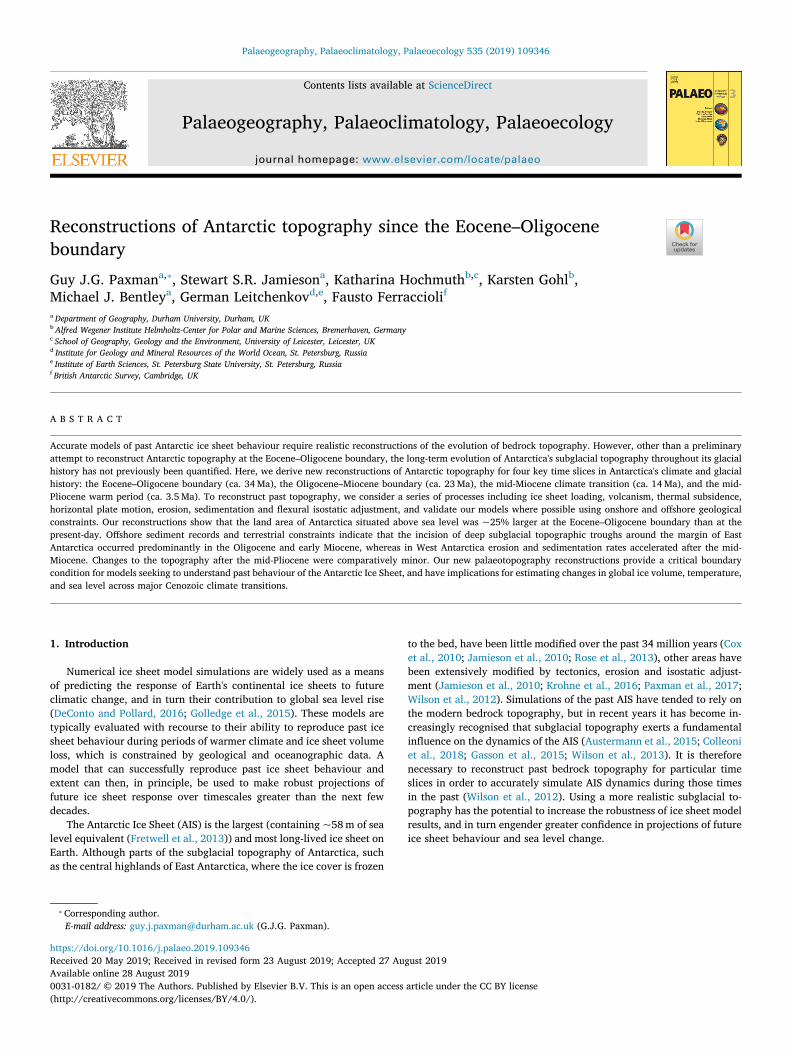
We build upon previous work by Wilson and Luyendyk (2009) andWilson et al. (2012) by beginning with the modern bedrock topographyof Antarctica (Fig. 1) and reversing a series of geological processes thathave acted to modify the topography since ca. 34Ma. We incorporate anumber of onshore and offshore datasets acquired or improved sincethese earlier reconstructions (see Section 3 and the supplementarymaterial), and give consideration to the rate at which the landscape hasevolved through time, rather than applying a simple linear interpola-tion between ca. 34Ma and the present-day (Gasson et al., 2016). For

Fig. 1. Present-day bedrock topography of Antarctica. Major topographic features referred to throughout the text are labelled. Italicised labels denote major floatingice shelves. Topography is given as elevation above mean sea level, and is contoured at 1 km intervals. The smooth area in Princess Elizabeth Land is indicative of adata-poor region. Black lines demarcate the modern grounding line and ice calving front. Red polygons highlight pre-glacial land surfaces exposed above the ice sheetor preserved beneath the ice. Yellow polygons highlight regions characterised by alpine topography with a clear fluvial signature (Baroni et al., 2005; Rose et al.,2013; Sugden et al., 2017). Numbered orange stars mark the locations of palaeo-elevation/uplift markers (Section 5.1). Dashed black polygons mark subglacialtrenches of inferred tectonic origin considered in our erosion model (Section 3.6.3); 1= Lake Vostok; 2=Adventure Subglacial Trench; 3=Astrolabe SubglacialTrench. Dashed magenta outline marks the approximate onshore location of the West Antarctic Rift System (WARS) (Bingham et al., 2012; Jordan et al., 2010).Abbreviations: BI= Berkner Island; EM=Ellsworth Mountains; LG= Lambert Graben; PM=Pensacola Mountains; SR=Shackleton Range; TM=Thiel Mountains.(For interpretation of the references to colour in this figure legend, the reader is referred to the web version of this article.)

G.J.G. Paxman, et al. Palaeogeography, Palaeoclimatology, Palaeoecology 535 (2019) 109346

2

each time slice, we produce a separate reconstruction of minimum andmaximum topography, which provide end-member scenarios that en-capsulate the cumulative uncertainties associated with each stage of thereconstruction process, and a median topography representing a‘middle-ground’ between the two end-members (Section 3). We refrainfrom addressing the evolution of the oceanic realm (i.e. beyond themodern continental shelf edge), since this is the main focus of on-goingwork on the reconstruction of the palaeobathymetry of the SouthernOcean (Hochmuth et al., in prep.).

3. Reconstruction methods

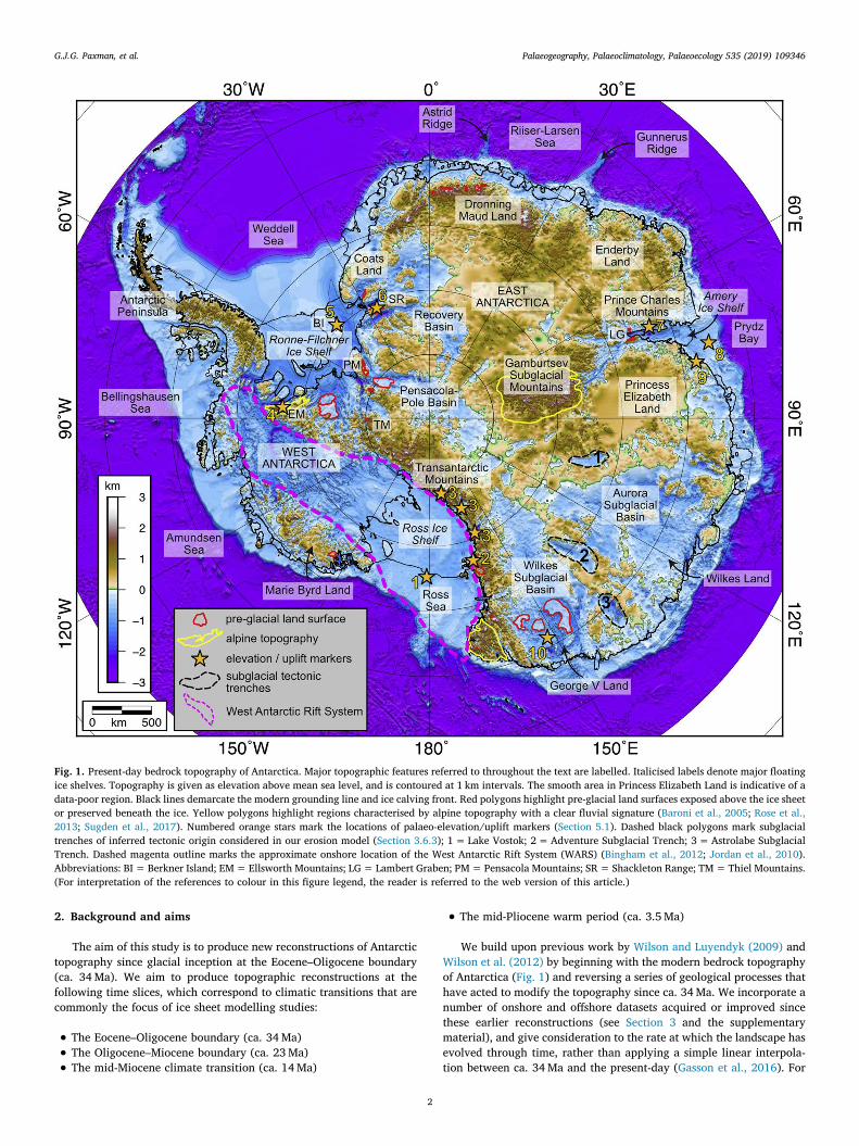
In this section we describe the steps involved in our topographicreconstruction in the order in which they were performed (as

summarised in Fig. 2). Several steps require the calculation of the iso-static response of the Antarctic lithosphere to surface load redistribu-tion, which is computed using an elastic plate model that accounts forspatial variability in flexural rigidity (Chen et al., 2018) (for detail seethe supplementary material). We also incorporate estimates of un-certainty associated with each step so as to construct minimum andmaximum topographies. The values of each parameter assumed in ourminimum, median and maximum reconstructions are shown in Sup-plementary Table 1. Each palaeotopography grid is produced at 5 kmhorizontal resolution and smoothed with a 10 km Gaussian filter toremove high frequency artefacts arising from the reconstruction pro-cess, without removing topographic features significantly larger thanthe grid resolution.

Fig. 2. Flow diagram of the topographic reconstruction process. Symbology: blue rectangles= input grids; red rhombs= elastic plate model used to computeflexural responses to load redistribution; yellow rectangles= outputs of flexural models; green rectangles= evolving bedrock topography DEMs. Note that theiteration scheme for calculating subsidence due to water loading is illustrated for the thermal subsidence step, but is also applied in each instance the elastic platemodel is used. (For interpretation of the references to colour in this figure legend, the reader is referred to the web version of this article.)

G.J.G. Paxman, et al. Palaeogeography, Palaeoclimatology, Palaeoecology 535 (2019) 109346

3

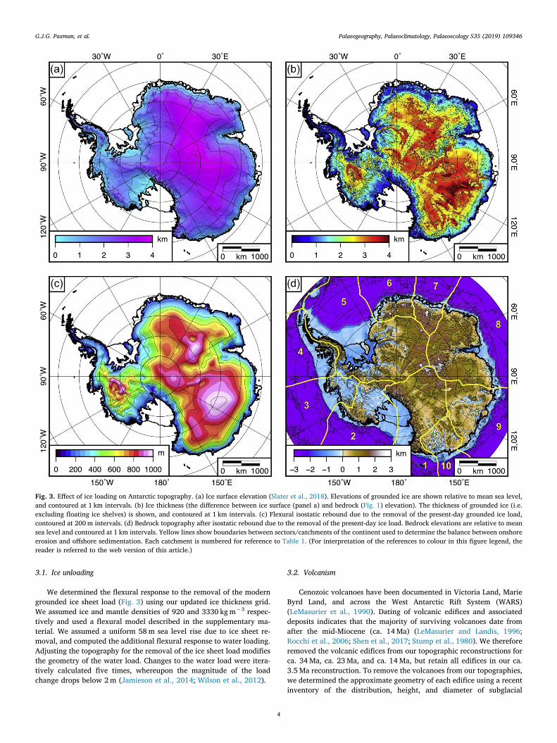
3.1. Ice unloading

We determined the flexural response to the removal of the moderngrounded ice sheet load (Fig. 3) using our updated ice thickness grid.We assumed ice and mantle densities of 920 and 3330 kgm−3 respec-tively and used a flexural model described in the supplementary ma-terial. We assumed a uniform 58m sea level rise due to ice sheet re-moval, and computed the additional flexural response to water loading.Adjusting the topography for the removal of the ice sheet load modifiesthe geometry of the water load. Changes to the water load were itera-tively calculated five times, whereupon the magnitude of the loadchange drops below 2m (Jamieson et al., 2014; Wilson et al., 2012).

3.2. Volcanism

Cenozoic volcanoes have been documented in Victoria Land, MarieByrd Land, and across the West Antarctic Rift System (WARS)(LeMasurier et al., 1990). Dating of volcanic edifices and associateddeposits indicates that the majority of surviving volcanoes date fromafter the mid-Miocene (ca. 14Ma) (LeMasurier and Landis, 1996;Rocchi et al., 2006; Shen et al., 2017; Stump et al., 1980). We thereforeremoved the volcanic edifices from our topographic reconstructions forca. 34Ma, ca. 23Ma, and ca. 14Ma, but retain all edifices in our ca.3.5Ma reconstruction. To remove the volcanoes from our topographies,we determined the approximate geometry of each edifice using a recentinventory of the distribution, height, and diameter of subglacial

Fig. 3. Effect of ice loading on Antarctic topography. (a) Ice surface elevation (Slater et al., 2018). Elevations of grounded ice are shown relative to mean sea level,and contoured at 1 km intervals. (b) Ice thickness (the difference between ice surface (panel a) and bedrock (Fig. 1) elevation). The thickness of grounded ice (i.e.excluding floating ice shelves) is shown, and contoured at 1 km intervals. (c) Flexural isostatic rebound due to the removal of the present-day grounded ice load,contoured at 200m intervals. (d) Bedrock topography after isostatic rebound due to the removal of the present-day ice load. Bedrock elevations are relative to meansea level and contoured at 1 km intervals. Yellow lines show boundaries between sectors/catchments of the continent used to determine the balance between onshoreerosion and offshore sedimentation. Each catchment is numbered for reference to Table 1. (For interpretation of the references to colour in this figure legend, thereader is referred to the web version of this article.)

G.J.G. Paxman, et al. Palaeogeography, Palaeoclimatology, Palaeoecology 535 (2019) 109346

4

volcanic cones across West Antarctica (van Wyk de Vries et al., 2018)(Fig. 4), and then subtracted these cones from the topography. Since thewavelength of these features is typically shorter than the flexural lengthscale of the lithosphere (Watts, 2001), we do not account for flexuralisostatic compensation of the edifices. Because the timing of volcanismis relatively well dated, we apply the same correction to each of ourminimum, median and maximum reconstructions. We also adjusted forthe adjacent uplift of the Marie Byrd Land dome (Section 3.7).

3.3. Horizontal plate motion

Although the relative motion between East and West Antarcticasince 34Ma is relatively minor, it is fairly well constrained by magneticanomaly offsets of ~75 km in the Ross Sea (Cande et al., 2000; Daveyet al., 2016). We follow Wilson and Luyendyk (2009) and Wilson et al.(2012) by applying a simple finite rotation to West Antarctica relativeto East Antarctica of 1.14° about a fixed Euler pole (71.5°S, 35.8°W)(Supplementary Fig. 2). This horizontal plate motion largely occurredin the Oligocene (Cande et al., 2000), so we apply the rotation to our ca.34Ma reconstruction, but not to subsequent time slices, since any post-23Ma rotations were likely small by comparison (Granot and Dyment,2018). The rotation was applied to each of our minimum, median andmaximum reconstructions.

3.4. Thermal subsidence

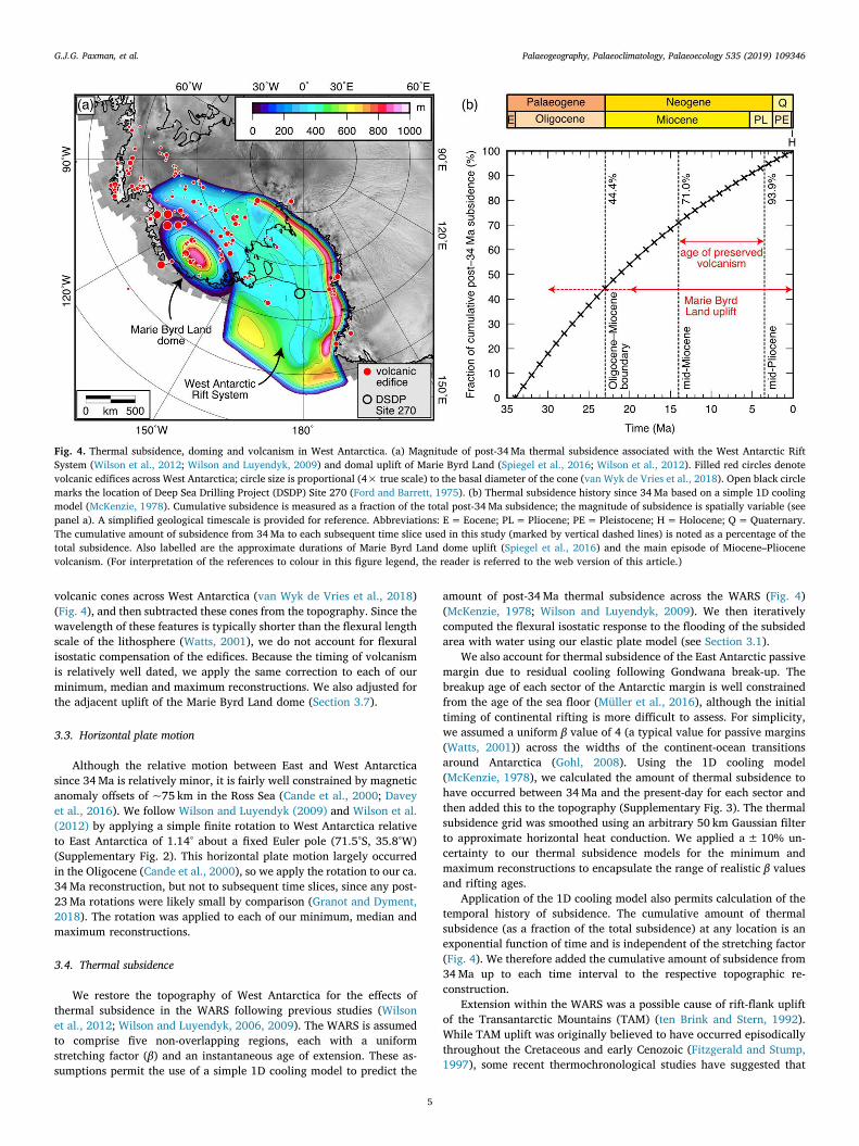
We restore the topography of West Antarctica for the effects ofthermal subsidence in the WARS following previous studies (Wilsonet al., 2012; Wilson and Luyendyk, 2006, 2009). The WARS is assumedto comprise five non-overlapping regions, each with a uniformstretching factor (β) and an instantaneous age of extension. These as-sumptions permit the use of a simple 1D cooling model to predict the

amount of post-34Ma thermal subsidence across the WARS (Fig. 4)(McKenzie, 1978; Wilson and Luyendyk, 2009). We then iterativelycomputed the flexural isostatic response to the flooding of the subsidedarea with water using our elastic plate model (see Section 3.1).

We also account for thermal subsidence of the East Antarctic passivemargin due to residual cooling following Gondwana break-up. Thebreakup age of each sector of the Antarctic margin is well constrainedfrom the age of the sea floor (Müller et al., 2016), although the initialtiming of continental rifting is more difficult to assess. For simplicity,we assumed a uniform β value of 4 (a typical value for passive margins(Watts, 2001)) across the widths of the continent-ocean transitionsaround Antarctica (Gohl, 2008). Using the 1D cooling model(McKenzie, 1978), we calculated the amount of thermal subsidence tohave occurred between 34Ma and the present-day for each sector andthen added this to the topography (Supplementary Fig. 3). The thermalsubsidence grid was smoothed using an arbitrary 50 km Gaussian filterto approximate horizontal heat conduction. We applied a± 10% un-certainty to our thermal subsidence models for the minimum andmaximum reconstructions to encapsulate the range of realistic β valuesand rifting ages.

Application of the 1D cooling model also permits calculation of thetemporal history of subsidence. The cumulative amount of thermalsubsidence (as a fraction of the total subsidence) at any location is anexponential function of time and is independent of the stretching factor(Fig. 4). We therefore added the cumulative amount of subsidence from34Ma up to each time interval to the respective topographic re-construction.

Extension within the WARS was a possible cause of rift-flank upliftof the Transantarctic Mountains (TAM) (ten Brink and Stern, 1992).While TAM uplift was originally believed to have occurred episodicallythroughout the Cretaceous and early Cenozoic (Fitzgerald and Stump,1997), some recent thermochronological studies have suggested that

Fig. 4. Thermal subsidence, doming and volcanism in West Antarctica. (a) Magnitude of post-34Ma thermal subsidence associated with the West Antarctic RiftSystem (Wilson et al., 2012; Wilson and Luyendyk, 2009) and domal uplift of Marie Byrd Land (Spiegel et al., 2016; Wilson et al., 2012). Filled red circles denotevolcanic edifices across West Antarctica; circle size is proportional (4× true scale) to the basal diameter of the cone (van Wyk de Vries et al., 2018). Open black circlemarks the location of Deep Sea Drilling Project (DSDP) Site 270 (Ford and Barrett, 1975). (b) Thermal subsidence history since 34Ma based on a simple 1D coolingmodel (McKenzie, 1978). Cumulative subsidence is measured as a fraction of the total post-34Ma subsidence; the magnitude of subsidence is spatially variable (seepanel a). A simplified geological timescale is provided for reference. Abbreviations: E= Eocene; PL= Pliocene; PE=Pleistocene; H=Holocene; Q=Quaternary.The cumulative amount of subsidence from 34Ma to each subsequent time slice used in this study (marked by vertical dashed lines) is noted as a percentage of thetotal subsidence. Also labelled are the approximate durations of Marie Byrd Land dome uplift (Spiegel et al., 2016) and the main episode of Miocene–Pliocenevolcanism. (For interpretation of the references to colour in this figure legend, the reader is referred to the web version of this article.)

G.J.G. Paxman, et al. Palaeogeography, Palaeoclimatology, Palaeoecology 535 (2019) 109346

5

the TAM may have experienced rapid uplift and denudation im-mediately after glacial inception at ca. 34Ma, resulting in the removalof the so-called ‘Mesozoic Victoria Basin’ (Lisker et al., 2014; Lisker andLäufer, 2013). Although this scenario remains subject to debate, it hasimplications for the regional palaeotopography at the Eocene–Oligo-cene boundary. However, the roles of thermal, erosional, tectonic andmantle-driven processes in driving TAM uplift remain poorly under-stood (Brenn et al., 2017; Paxman et al., 2019; Stern et al., 2005). Wetherefore make a simple adjustment to our minimum ca. 34Ma

palaeotopography by halving the elevation of the TAM following theadjustments for erosion and the associated flexural uplift (Section 3.6).This resulted in TAM palaeo-elevations comparable to those of thehinterland, in keeping with the end-member scenario of the possiblepresence of a pre-glacial sedimentary basin.

3.5. Offshore sedimentation

Sediment thicknesses on the continental shelf and in the deep sea

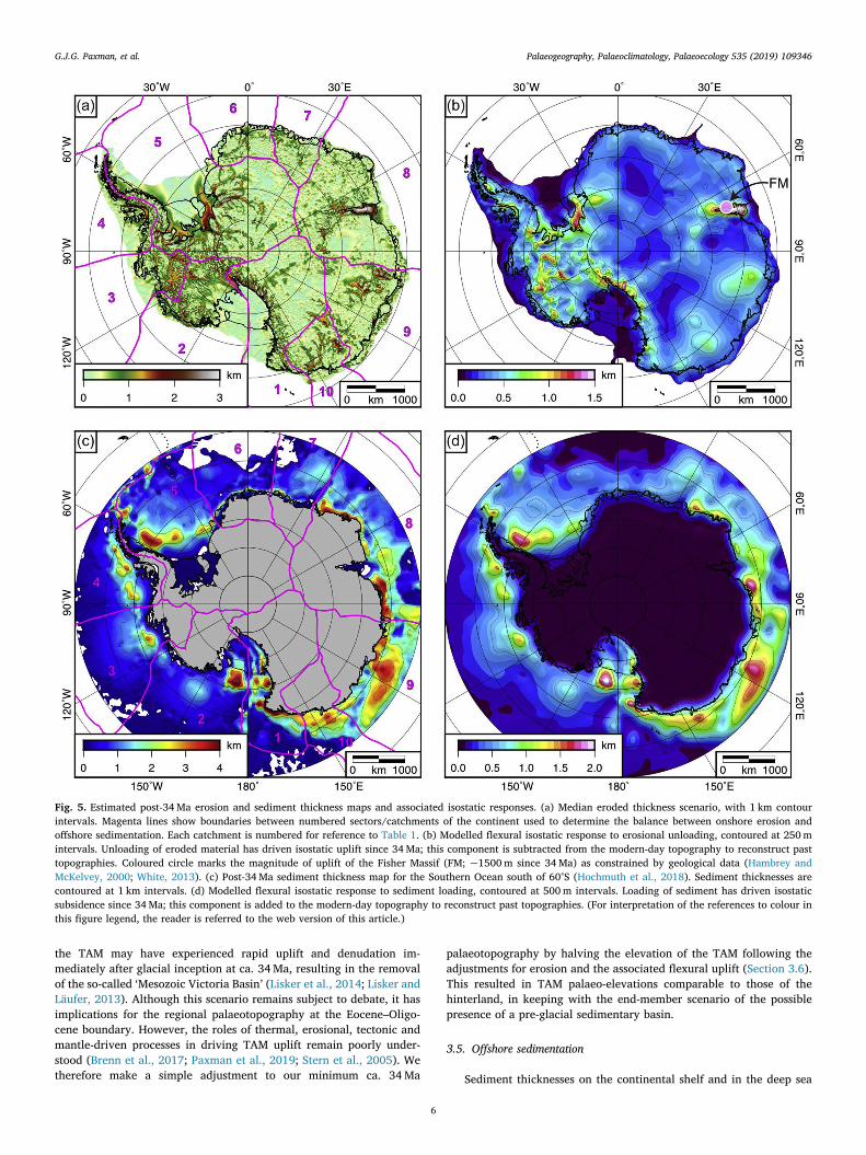
Fig. 5. Estimated post-34Ma erosion and sediment thickness maps and associated isostatic responses. (a) Median eroded thickness scenario, with 1 km contourintervals. Magenta lines show boundaries between numbered sectors/catchments of the continent used to determine the balance between onshore erosion andoffshore sedimentation. Each catchment is numbered for reference to Table 1. (b) Modelled flexural isostatic response to erosional unloading, contoured at 250mintervals. Unloading of eroded material has driven isostatic uplift since 34Ma; this component is subtracted from the modern-day topography to reconstruct pasttopographies. Coloured circle marks the magnitude of uplift of the Fisher Massif (FM; ~1500m since 34Ma) as constrained by geological data (Hambrey andMcKelvey, 2000; White, 2013). (c) Post-34Ma sediment thickness map for the Southern Ocean south of 60°S (Hochmuth et al., 2018). Sediment thicknesses arecontoured at 1 km intervals. (d) Modelled flexural isostatic response to sediment loading, contoured at 500m intervals. Loading of sediment has driven isostaticsubsidence since 34Ma; this component is added to the modern-day topography to reconstruct past topographies. (For interpretation of the references to colour inthis figure legend, the reader is referred to the web version of this article.)

G.J.G. Paxman, et al. Palaeogeography, Palaeoclimatology, Palaeoecology 535 (2019) 109346

6

were derived from a recent compilation of reflection seismic data(Hochmuth et al., 2018; Straume et al., 2019) (Fig. 5; for details see thesupplementary material). The thickness (and mass) of offshore sedi-ment can be used to (a) reconstruct the palaeobathymetry of the con-tinental shelf and rise, and (b) constrain the mass of onshore erosion(Section 3.6). To produce each of our reconstructions, we removed allstratigraphic units younger than the time slice of interest, and sub-tracted or added the associated sediment thickness uncertainty (Sup-plementary Fig. 5) in our minimum and maximum topographies re-spectively.

3.5.1. Compaction modelWe computed the flexural isostatic response to sediment loading

using our elastic plate model. The density of shelf sediments varies withdepth owing to mechanical compaction and reduction of porosity dueto the overburden pressure. We used a simple compaction model toestimate the variation of sediment density with depth, whereby thedecrease in sediment porosity (Φ) with increasing depth in the column(z) is given by an empirical exponential function (Sclater and Christie,1980)

=z z( ) exp0 (1)

where Φ0 is the initial porosity and λ is the compaction decay lengthscale. We then determined the depth-averaged effective density ( eff ) ofsediment around the Antarctic margin by removing the contributionfrom pore water, which is not restored to the continent.

=x y x yz x y

z x y( , ) ( , ) 1( , )

1 exp ( , )eff s

max

max0

(2)

where ρs is the density of the sediment grains, and zmax is the totalthickness of sediment being considered. For our median scenario, weassumed a grain density of 2600 kgm−3 for sediment on the continentalshelf, and 2400 kgm−3 for deep-sea sediments (Sclater and Christie,1980). We used values of 0.7 for the initial porosity and 1.0 km for thecompaction decay length scale, based on empirical porosity-depthcurves for Antarctic shelf sediments (Barker and Kennett, 1988; Escutiaet al., 2011). We then used a realistic range of values for these para-meters in our minimum and maximum reconstructions (SupplementaryTable 1).

3.5.2. Terrigenous fractionWe estimated the fraction of offshore sediment that was derived

from the continent as opposed to biogenic or pelagic material. Wecompared smear slide analysis from IODP/ODP/DSDP drill coresaround the Antarctic margin representing the main sedimentary en-vironments within the Southern Ocean (Barker and Kennett, 1988;Barker, 1999; Escutia et al., 2011). These data indicated that on thecontinental shelf, ~5% of material was biogenic, and the remaining~95% was terrigenous in origin. In the deep ocean realm, ~70% ofmaterial from the Miocene to present is terrigenous, but this fractionincreases to ~95% in the Oligocene. Although the spatial coverage ofdrill cores is sparse, and some localised variability is observed, thisgeneral trend is consistently observed. We therefore used the aboveaverage values, with± 5% uncertainty bounds to encapsulate the ma-jority of the spatial variability, around the entire margin. This is a moredetailed terrigenous fraction model than that used in the earlier re-constructions by Wilson et al. (2012).

3.5.3. Catchment boundariesWhen restoring sedimentary material to the continent and com-

paring the mass balance between erosion and sedimentation, it is im-portant to consider the provenance of the offshore sediments. Wetherefore investigated whether offshore sediment around the Antarcticmargin could be spatially sub-divided based on the geographic origin of

the sediment. We sub-divided the sediment into ten sectors/catchmentsbased on (a) boundaries mapped using geochemical provenance tracerssuch as 40Ar/39Ar ages and Nd isotopic compositions (e.g. Cook et al.,2013); (b) bathymetric ‘highs’ that form natural boundaries betweenseparate basins on the continental shelf, such as Gunnerus Ridge andAstrid Ridge (Fig. 1) (Eagles et al., 2018); and (c) structural/basementhighs observed in seismic data that may reflect geological boundaries,such as the Ross Sea Central High (Decesari et al., 2007).

We traced our assumed catchment boundaries over these previouslydocumented features, and continued the boundaries inland based onobserved ice surface velocity (Rignot et al., 2011) and bedrock drainagedivides (Jamieson et al., 2014) (Figs. 2, 5). Our approach was to sub-divide only if the boundary clearly met one of the above three criteria.The area of the sub-divided catchments therefore varies by up to oneorder of magnitude. We computed the minimum, median and maximummass of post-34Ma sediment for each catchment for comparison withour erosion estimate (Section 3.6).

3.6. Erosion restoration

3.6.1. Identification of pre-glacial landscapesThe morphology of the Antarctic landscape is a record of the surface

processes that have acted upon it over geological timescales. To esti-mate the spatial distribution of glacial erosion across the continent, weidentified landscapes or ‘reference’ relict surfaces that have been largelyunmodified by large-scale glaciation, and have therefore experiencednegligible erosion since ca. 34Ma (Fig. 1). Such landscapes includeundulating plateau surfaces exposed in highlands (Näslund, 2001;White, 2013) and observed beneath the ice around the Weddell SeaEmbayment and within the Wilkes Subglacial Basin (Paxman et al.,2018; Rose et al., 2015), and alpine landscapes in the GamburtsevSubglacial Mountains (GSM) (Paxman et al., 2016; Rose et al., 2013),Dronning Maud Land (DML) (Näslund, 2001), and the TAM (Sugdenet al., 1999). In these regions, we assumed that the preserved mountainpeaks have not experienced significant denudation or modificationsince ca. 34Ma. Moreover, relatively unmodified fluvial valley systemsare preserved in the northern TAM (Baroni et al., 2005; Sugden et al.,1995) and Ellsworth Mountains (Sugden et al., 2017), and the large-scale continental fluvial structure is still visible in the landscape today(Jamieson et al., 2014; Sugden and Jamieson, 2018).

3.6.2. Summit accordanceWe consider glacial erosion to comprise two components: (1) se-

lective linear erosion (valley/trough incision), and (2) uniform surfacelowering via areal scour (Molnar and England, 1990; Sugden and John,1976).

To estimate the spatial distribution of glacial valley incision, weassumed that pre-glacial landscape features identified across Antarcticaonce formed part of a contiguous surface prior to glacial incision. Sincethese pre-glacial land surfaces are sparsely distributed, we also identi-fied local topographic ‘highs’ within a circular moving window(Champagnac et al., 2007). The diameter of the moving window was setto 30 km to capture the width of large subglacial troughs. We then in-terpolated a smooth continuous surface between all surfaces/summits,which are assumed to have not experienced significant erosion sinceAIS inception at 34Ma. The resulting summit accordance surface(Supplementary Fig. 6) represents the restoration of eroded material tothe topography without accounting for the associated isostatic response(Champagnac et al., 2007). The difference between the summit ac-cordance surface and the bedrock topography represents our estimateof selective glacial incision (sometimes referred to as the ‘geophysicalrelief’ (Champagnac et al., 2007)).

In parts of Antarctica such as the GSM and TAM, a pre-existingfluvial landscape has been modified by alpine-style glaciation, and isnow preserved beneath non-erosive ice (Sugden and Jamieson, 2018).By completely filling the valleys in these regions, we would likely

G.J.G. Paxman, et al. Palaeogeography, Palaeoclimatology, Palaeoecology 535 (2019) 109346

7

overestimate the amount of post-34Ma erosion, and therefore producean unrealistically smooth palaeolandscape. Mapping of glacial over-deepenings within the GSM indicates that glacial erosion accountsfor––to first order––approximately 50% of the total volume of valleyincision (Rose et al., 2013). We therefore decreased the predictedthickness of valley incision in these alpine landscapes by 50% in ourerosion model. The result is a pre-glacial landscape that preserves theinherited fluvial valley network that was subsequently exploited byearly ice sheets (Sugden and Jamieson, 2018; Sugden and John, 1976).We also adjusted the summit accordance surface and erosion estimatefor deep subglacial trenches whose relief may, in part, be explained bytectonic subsidence as well as (or as opposed to) glacial erosion (see thesupplementary material).

Accounting for valley incision alone will produce a minimum esti-mate of erosion, since it assumes that the peaks between the valleyshave not been eroded. However, uniform surface lowering of the peakssince ca. 34Ma is largely unconstrained by geomorphology. As a simplesolution, we tuned the magnitude of uniform surface lowering toachieve as close a match as possible between the mass of eroded ma-terial and offshore sediment within each catchment for our minimum,median and maximum scenarios, while avoiding abrupt ‘steps’ ineroded thickness across catchment boundaries (Fig. 5; SupplementaryFig. 7; Table 1; Supplementary Table 2).

3.6.3. Eroded bedrock density and flexureThe subglacial geology of Antarctica, and therefore the density of

the eroded bedrock, is almost entirely unconstrained. However, EastAntarctica can be broadly considered to comprise a suite of rocks fromhigher-density Proterozoic and Archean metamorphic and magmaticbasement (Boger, 2011; Ferraccioli et al., 2011; Goodge et al., 2017) tolower-density Palaeozoic sandstones (Barrett, 1991; Elliot et al., 2015).We therefore assumed a range of densities in East Antarctica from 2400to 2800 kgm−3 for our minimum and maximum reconstructions, and2600 kgm−3 as a realistic average. In West Antarctica, we assumed arange of 2200 to 2600 kgm−3 to reflect the higher proportion of Me-sozoic or younger sedimentary rocks (Studinger et al., 2001), with2400 kgm−3 as a realistic average. We then computed the flexuralisostatic adjustment to erosional unloading using our elastic platemodel. To correct the topography for the effects of erosion, we addedthe estimated post-34Ma eroded thickness to the topography, andsubtracted the associated flexural response.

3.6.4. Rates of erosion and sedimentationTo reconstruct topography at intermediate time slices, it was ne-

cessary to quantify the variation in erosion and sedimentation ratesover time. We collated constraints on sedimentation rates from seismicreflection profiles and ocean sediment drill cores (Barker and Kennett,1988; Escutia et al., 2011), assuming that sediment thickness dependson sedimentation rate alone, which in turn is a proxy for onshore ero-sion rates. We used these offshore sediment data together with onshoreerosion rate constraints to estimate an erosion and sedimentation his-tory for each of the ten catchments (Table 1), which we then used torestore the appropriate amount of eroded material/sediment betweeneach time slice. In our reconstructions, we made the assumption thatthe catchment boundaries have remained constant over time, since thefirst-order topographic controls on Antarctic drainage patterns (e.g. theGSM and TAM) predate ice sheet inception (Rose et al., 2013), and theoverall subglacial drainage pattern is continentally radial, and thereforedrainage re-organisation is not expected to have occurred on a largescale (Sugden and Jamieson, 2018). We also assume that the offshoresediment boundaries have remained fixed over time, and that lateraltransport of sediment by circumpolar currents is unlikely to have oc-curred in large volumes.

3.7. Dynamic topography

Long wavelength changes in bedrock elevation in Antarctica may, inpart, be driven by vertical tractions exerted on the base of the litho-sphere by the convecting mantle (i.e. dynamic topography). Changes indynamic topography since the Eocene have been inferred in parts ofAntarctica such as the Ross Sea, Wilkes Subglacial Basin and Marie ByrdLand (Austermann et al., 2015; LeMasurier and Landis, 1996). Sincemodels of past mantle convection patterns are currently poorly con-strained in space and time, we do not attempt to incorporate thesechanges here, with the exception of the post-34Ma dynamic uplift ofthe Marie Byrd Land dome (Fig. 4).

We followed Wilson et al. (2012) by subtracting an ellipticalGaussian dome of 1000 km×500 km diameter (Fig. 4) with a max-imum amplitude of 1 km (LeMasurier and Landis, 1996) from ourmedian ca. 34Ma palaeotopography. We then corrected the more re-cent palaeotopographies assuming that uplift commenced at ca. 20Maand proceeded linearly to the present-day (Fig. 4), as indicated by re-cent thermochronology data (Spiegel et al., 2016). However, only fourfission track ages were acquired from Marie Byrd Land, resulting in alarge uncertainty in the ca. 20Ma estimate (Spiegel et al., 2016). Weallow for this uncertainty by changing the maximum amplitude ofdomal uplift to 2000m and the beginning of uplift to ca. 30Ma in ourminimum reconstruction (Fig. 4) (LeMasurier and Landis, 1996; Rocchiet al., 2006), and foregoing this adjustment altogether in our maximumreconstruction.

We note that future robust models of post-34Ma dynamic topo-graphy change across Antarctica can readily incorporated into our pa-laeotopographic reconstructions.

4. Results

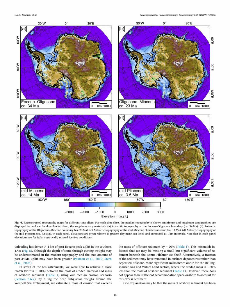
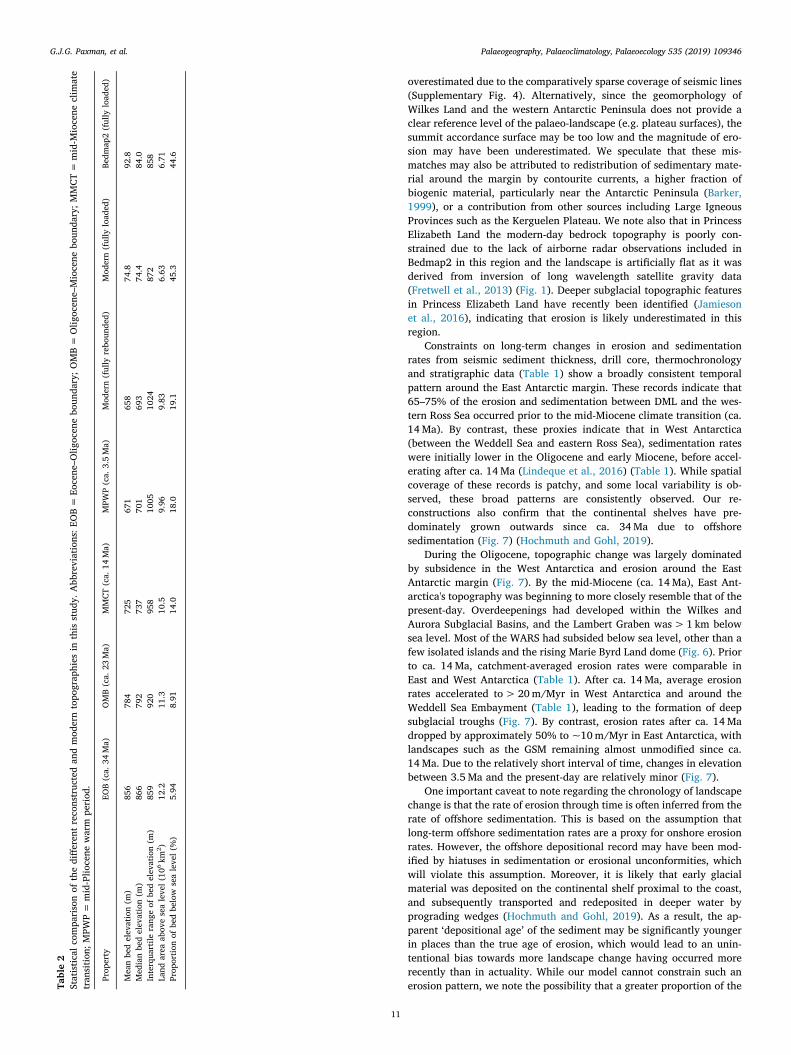
The results of our reconstruction process are new topographies atfour time slices between the Eocene–Oligocene boundary and mid-Pliocene warm period (Fig. 6). We find that the average bed elevationof Antarctica has decreased by ~200m between ca. 34Ma and thepresent-day (Table 2), and the interquartile range of bed elevations (arough measure of topographic relief) has increased by ~200m(Table 2). These changes are attributed largely to thermal subsidence,focussed erosion in deep subglacial troughs, and concomitant flexuraluplift of the flanking regions. The increase in topographic relief isvisible in the new palaeo-DEMs (Fig. 6), with an increasing fraction ofthe bed dropping below sea level (Supplementary Fig. 8). The area ofland above sea level at ca. 34Ma is 12.2× 106 km2, with ~6% of thebed situated below sea level, as opposed to 9.83×106 km2 and ~19%respectively at the present-day (Table 2). These figures refer to themedian topographies in each case; the minimum and maximum topo-graphies are shown in Supplementary Figs. 9 and 10.

The most significant changes in elevation in East Antarctica occurwithin the Wilkes, Aurora, Recovery and Lambert basins, which werelow-lying but predominately situated at 0–500m above sea level priorto glacial inception (Fig. 6). Prior to thermal subsidence and erosion, asignificant area of West Antarctica underlain by the WARS was alsosituated up to 500m above sea level (Fig. 6). The Weddell Sea was a500–1000m deep embayment, the shallow extremities of which mayhave extended up to a few hundred km inland of the modern-daygrounding line. The Ross Sea comprised a series of elongate horst andgraben-like features, with topographic ‘highs’ such as the Central Highsituated at or just above sea level (Fig. 6). Our reconstruction retainsthe major highlands within East Antarctica, such as the GSM, TAM, andthe escarpment in DML, with the GSM the highest feature at up to2.5 km above sea level at ca. 34Ma (Fig. 6). Because we only partiallyfilled the valleys within the GSM, the pre-existing fluvial network canbe seen in the ca. 34Ma reconstruction. However, the through-cuttingtroughs that characterise the modern TAM have largely been filled inour reconstruction (Fig. 6). Our flexural models indicate that erosional

G.J.G. Paxman, et al. Palaeogeography, Palaeoclimatology, Palaeoecology 535 (2019) 109346

8

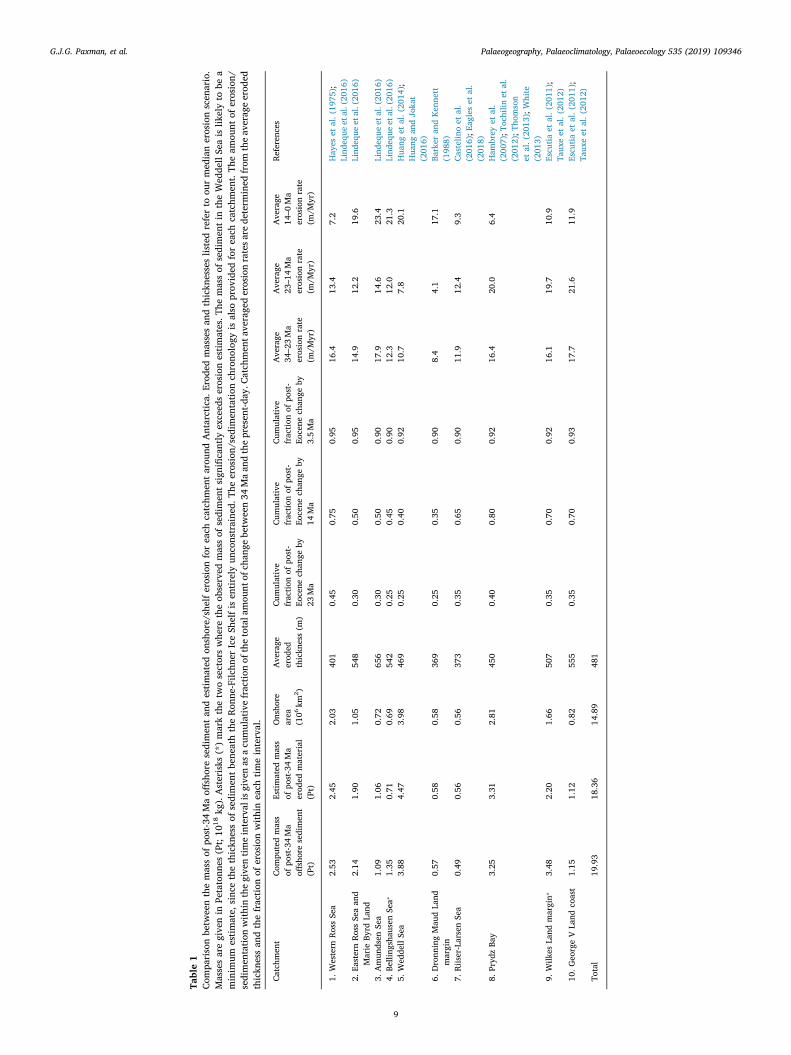
Table1

Compa

risonbe

twee

nthemassof

post-34Maoff

shoresedimen

tan

destim

ated

onsh

ore/

shelfe

rosion

forea

chca

tchm

enta

roun

dAntarctica.

Erod

edmassesan

dthickn

esseslis

tedreferto

ourmed

ianerosionscen

ario.

Massesaregive

nin

Petatonn

es(Pt;10

18kg

).Asterisks

(*)markthetw

osectorswhe

retheob

served

massof

sedimen

tsignific

antly

exceed

serosionestim

ates.T

hemassof

sedimen

tintheWed

dellSe

ais

likelyto

bea

minim

umestim

ate,

sinc

ethethickn

essof

sedimen

tben

eath

theRo

nne-Filchn

erIceSh

elfisen

tirelyun

constraine

d.Th

eerosion/

sedimen

tatio

nch

rono

logy

isalso

prov

ided

forea

chca

tchm

ent.Th

eam

ount

oferosion/

sedimen

tatio

nwith

inthegive

ntim

einterval

isgive

nas

acu

mulativefrac

tionof

thetotala

mou

ntof

chan

gebe

twee

n34

Maan

dthepresen

t-day

.Catch

men

tave

rage

derosionratesa

rede

term

ined

from

theav

erag

eerod

edthickn

essan

dthefrac

tionof

erosionwith

inea

chtim

einterval.

Catchm

ent

Compu

tedmass

ofpo

st-34Ma

offsh

oresedimen

t(Pt)

Estim

ated

mass

ofpo

st-34Ma

erod

edmaterial

(Pt)

Onsho

rearea

(106

km2 )

Ave

rage

erod

edthickn

ess(m

)

Cumulative

frac

tionof

post-

Eocene

chan

geby

23Ma

Cumulative

frac

tionof

post-

Eocene

chan

geby

14Ma

Cumulative

frac

tionof

post-

Eocene

chan

geby

3.5Ma

Ave

rage

34–2

3Ma

erosionrate

(m/M

yr)

Ave

rage

23–1

4Ma

erosionrate

(m/M

yr)

Ave

rage

14–0

Ma

erosionrate

(m/M

yr)

Referenc

es

1.Western

Ross

Sea

2.53

2.45

2.03

401

0.45

0.75

0.95

16.4

13.4

7.2

Hay

eset

al.(

1975

);Lind

eque

etal.(20

16)

2.Ea

sternRo

ssSe

aan

dMarie

Byrd

Land

2.14

1.90

1.05

548

0.30

0.50

0.95

14.9

12.2

19.6

Lind

eque

etal.(20

16)

3.Amun

dsen

Sea

1.09

1.06

0.72

656

0.30

0.50

0.90

17.9

14.6

23.4

Lind

eque

etal.(20

16)

4.Be

lling

shau

senSe

a⁎1.35

0.71

0.69

542

0.25

0.45

0.90

12.3

12.0

21.3

Lind

eque

etal.(20

16)

5.Wed

dellSe

a3.88

4.47

3.98

469

0.25

0.40

0.92

10.7

7.8

20.1

Hua

nget

al.(

2014

);Hua

ngan

dJo

kat

(201

6)6.

Dronn

ingMau

dLa

ndmargin

0.57

0.58

0.58

369

0.25

0.35

0.90

8.4

4.1

17.1

Barker

andKe

nnett

(198

8)7.

Riiser-LarsenSe

a0.49

0.56

0.56

373

0.35

0.65

0.90

11.9

12.4

9.3

Castelinoet

al.

(201

6);E

agleset

al.

(201

8)8.

Pryd

zBa

y3.25

3.31

2.81

450

0.40

0.80

0.92

16.4

20.0

6.4

Ham

brey

etal.

(200

7);T

ochilin

etal.

(201

2);T

homson

etal.(

2013

);White

(201

3)9.

Wilk

esLa

ndmargin⁎

3.48

2.20

1.66

507

0.35

0.70

0.92

16.1

19.7

10.9

Escu

tiaet

al.(

2011

);Ta

uxeet

al.(

2012

)10

.Geo

rgeV

Land

coast

1.15

1.12

0.82

555

0.35

0.70

0.93

17.7

21.6

11.9

Escu

tiaet

al.(

2011

);Ta

uxeet

al.(

2012

)To

tal

19.93

18.36

14.89

481

G.J.G. Paxman, et al. Palaeogeography, Palaeoclimatology, Palaeoecology 535 (2019) 109346

9

unloading has driven>1 km of post-Eocene peak uplift in the southernTAM (Fig. 5), although the depth of some through-cutting troughs maybe underestimated in the modern topography and the true amount ofpost-34Ma uplift may have been greater (Paxman et al., 2019; Sternet al., 2005).

In seven of the ten catchments, we were able to achieve a closematch (within±10%) between the mass of eroded material and massof offshore sediment (Table 1) using our median erosion scenario(Section 3.6.2). By filling the deep subglacial troughs around theWeddell Sea Embayment, we estimate a mass of erosion that exceeds

the mass of offshore sediment by ~20% (Table 1). This mismatch in-dicates that we may be missing a small but significant volume of se-diment beneath the Ronne-Filchner Ice Shelf. Alternatively, a fractionof the sediment may have remained in onshore depocentres rather thandeposited offshore. More significant mismatches occur for the Belling-shausen Sea and Wilkes Land sectors, where the eroded mass is ~50%less than the mass of offshore sediment (Table 1). However, there doesnot appear to be sufficient accommodation space onshore to account forthis excess sediment.

One explanation may be that the mass of offshore sediment has been

Fig. 6. Reconstructed topography maps for different time slices. For each time slice, the median topography is shown (minimum and maximum topographies aredisplayed in, and can be downloaded from, the supplementary material). (a) Antarctic topography at the Eocene–Oligocene boundary (ca. 34Ma). (b) Antarctictopography at the Oligocene–Miocene boundary (ca. 23Ma). (c) Antarctic topography at the mid-Miocene climate transition (ca. 14Ma). (d) Antarctic topography atthe mid-Pliocene (ca. 3.5Ma). In each panel, elevations are given relative to present-day mean sea level, and contoured at 1 km intervals. Note that in each panelelevations are for fully isostatically relaxed ice-free conditions.

G.J.G. Paxman, et al. Palaeogeography, Palaeoclimatology, Palaeoecology 535 (2019) 109346

10

overestimated due to the comparatively sparse coverage of seismic lines(Supplementary Fig. 4). Alternatively, since the geomorphology ofWilkes Land and the western Antarctic Peninsula does not provide aclear reference level of the palaeo-landscape (e.g. plateau surfaces), thesummit accordance surface may be too low and the magnitude of ero-sion may have been underestimated. We speculate that these mis-matches may also be attributed to redistribution of sedimentary mate-rial around the margin by contourite currents, a higher fraction ofbiogenic material, particularly near the Antarctic Peninsula (Barker,1999), or a contribution from other sources including Large IgneousProvinces such as the Kerguelen Plateau. We note also that in PrincessElizabeth Land the modern-day bedrock topography is poorly con-strained due to the lack of airborne radar observations included inBedmap2 in this region and the landscape is artificially flat as it wasderived from inversion of long wavelength satellite gravity data(Fretwell et al., 2013) (Fig. 1). Deeper subglacial topographic featuresin Princess Elizabeth Land have recently been identified (Jamiesonet al., 2016), indicating that erosion is likely underestimated in thisregion.

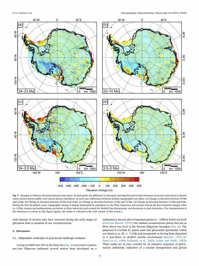
Constraints on long-term changes in erosion and sedimentationrates from seismic sediment thickness, drill core, thermochronologyand stratigraphic data (Table 1) show a broadly consistent temporalpattern around the East Antarctic margin. These records indicate that65–75% of the erosion and sedimentation between DML and the wes-tern Ross Sea occurred prior to the mid-Miocene climate transition (ca.14Ma). By contrast, these proxies indicate that in West Antarctica(between the Weddell Sea and eastern Ross Sea), sedimentation rateswere initially lower in the Oligocene and early Miocene, before accel-erating after ca. 14Ma (Lindeque et al., 2016) (Table 1). While spatialcoverage of these records is patchy, and some local variability is ob-served, these broad patterns are consistently observed. Our re-constructions also confirm that the continental shelves have pre-dominately grown outwards since ca. 34Ma due to offshoresedimentation (Fig. 7) (Hochmuth and Gohl, 2019).

During the Oligocene, topographic change was largely dominatedby subsidence in the West Antarctica and erosion around the EastAntarctic margin (Fig. 7). By the mid-Miocene (ca. 14Ma), East Ant-arctica's topography was beginning to more closely resemble that of thepresent-day. Overdeepenings had developed within the Wilkes andAurora Subglacial Basins, and the Lambert Graben was>1 km belowsea level. Most of the WARS had subsided below sea level, other than afew isolated islands and the rising Marie Byrd Land dome (Fig. 6). Priorto ca. 14Ma, catchment-averaged erosion rates were comparable inEast and West Antarctica (Table 1). After ca. 14Ma, average erosionrates accelerated to>20m/Myr in West Antarctica and around theWeddell Sea Embayment (Table 1), leading to the formation of deepsubglacial troughs (Fig. 7). By contrast, erosion rates after ca. 14Madropped by approximately 50% to ~10m/Myr in East Antarctica, withlandscapes such as the GSM remaining almost unmodified since ca.14Ma. Due to the relatively short interval of time, changes in elevationbetween 3.5Ma and the present-day are relatively minor (Fig. 7).

One important caveat to note regarding the chronology of landscapechange is that the rate of erosion through time is often inferred from therate of offshore sedimentation. This is based on the assumption thatlong-term offshore sedimentation rates are a proxy for onshore erosionrates. However, the offshore depositional record may have been mod-ified by hiatuses in sedimentation or erosional unconformities, whichwill violate this assumption. Moreover, it is likely that early glacialmaterial was deposited on the continental shelf proximal to the coast,and subsequently transported and redeposited in deeper water byprograding wedges (Hochmuth and Gohl, 2019). As a result, the ap-parent ‘depositional age’ of the sediment may be significantly youngerin places than the true age of erosion, which would lead to an unin-tentional bias towards more landscape change having occurred morerecently than in actuality. While our model cannot constrain such anerosion pattern, we note the possibility that a greater proportion of theTa

ble2

Statistic

alco

mpa

risonof

thediffe

rent

reco

nstruc

tedan

dmod

erntopo

grap

hies

inthis

stud

y.Abb

reviations:E

OB=

Eocene

–Olig

ocen

ebo

unda

ry;O

MB=

Olig

ocen

e–Miocene

boun

dary;M

MCT

=mid-M

iocene

clim

ate

tran

sitio

n;MPW

P=

mid-Plio

cene

warm

period

.

Prop

erty

EOB(ca.

34Ma)

OMB(ca.

23Ma)

MMCT

(ca.

14Ma)

MPW

P(ca.

3.5Ma)

Mod

ern(fully

rebo

unde

d)Mod

ern(fully

load

ed)

Bedm

ap2(fully

load

ed)

Mea

nbe

delev

ation(m

)85

678

472

567

165

874

.892

.8Med

ianbe

delev

ation(m

)86

679

273

770

169

374

.484

.0Interqua

rtile

rang

eof

bedelev

ation(m

)85

992

095

810

0510

2487

285

8La

ndarea

abov

esealeve

l(10

6km

2 )12

.211

.310

.59.96

9.83

6.63

6.71

Prop

ortio

nof

bedbe

low

sealeve

l(%)

5.94

8.91

14.0

18.0

19.1

45.3

44.6

G.J.G. Paxman, et al. Palaeogeography, Palaeoclimatology, Palaeoecology 535 (2019) 109346

11

total amount of erosion may have occurred during the early stages ofglaciation than is assumed in our reconstructions.

5. Discussion

5.1. Independent constraints on post-Eocene landscape evolution

Coring at DSDP Site 270 in the Ross Sea (Fig. 4) recovered a maturepre-Late Oligocene palaeosol several metres deep developed on a

sedimentary breccia above basement gneiss at ~1000m below sea level(Ford and Barrett, 1975). Our median reconstruction places this site at80m above sea level at the Eocene–Oligocene boundary (Fig. 6). Thepalaeosol is overlain by quartz sand and glauconitic greensand, whichare dated at ca. 26 ± 1.5Ma and interpreted as having been depositedin a near-shore or shallow marine environment (Barrett, 1975; DeSantis et al., 1999; Kulhanek et al., 2019; Leckie and Webb, 1983).These sands are in turn overlain by an extensive sequence of glacio-marine sediments, indicative of a marine transgression and glacial

Fig. 7. Changes in bedrock elevation between time slices. In each panel, the difference in elevation (moving forward in time) between successive time slices is shown;warm colours denote uplift; cool colours denote subsidence. In each case, differences between median topographies are taken. (a) Change in elevation between 34Maand 23Ma. (b) Change in elevation between 23Ma and 14Ma. (c) Change in elevation between 14Ma and 3.5Ma. (d) Change in elevation between 3.5Ma and 0Ma.During the first 20 million years, topographic change is largely dominated by subsidence in the West Antarctica and erosion around the East Antarctic margin. Afterca. 14Ma, erosion and sedimentation accelerate in West Antarctica and around the Weddell Sea Embayment, and decelerate in East Antarctica. (For interpretation ofthe references to colour in this figure legend, the reader is referred to the web version of this article.)

G.J.G. Paxman, et al. Palaeogeography, Palaeoclimatology, Palaeoecology 535 (2019) 109346

12

expansion (Kulhanek et al., 2019). Our median reconstruction indicatesthat this site subsided below sea level at ca. 28Ma, which is in goodagreement with the observed stratigraphy. In our minimum re-construction (Supplementary Fig. 9), the site is already below sea levelat ca. 34Ma, whereas in our maximum reconstruction (SupplementaryFig. 10), the site does not subside below sea level until ca. 21Ma. Thishighlights the conservative nature of our minimum and maximum re-constructions.

On the Fisher Massif in the Prince Charles Mountains (Fig. 5), post-Eocene fjordal sediments of the Pagodroma Group deposited close tosea level are exposed at up to 1.5 km above present-day sea level(Hambrey and McKelvey, 2000; White, 2013; Whitehead et al., 2003).Moreover, the age of Pagodroma Group deposits increases system-atically with increasing elevation. Our erosion and flexure modelssuggest that up to 3 km of glacial excavation within the Lambert Grabenhas driven up to 1.4 km of flexural uplift along the graben flanks, whichis within 100m of the elevation of the oldest Pagodroma Group sedi-ments. Combined with thermochronology data (Thomson et al., 2013;Tochilin et al., 2012), the observed apparent ‘inverted stratigraphy’ ofthe Pagodroma Group indicates a period of enhanced denudation inOligocene and early Miocene times, and that flexural uplift has oc-curred throughout the Cenozoic and contemporaneous with fjordalsedimentation. We also note that matching this observational constraintis only possible if a relatively low (compared to other parts of EastAntarctica) effective elastic thickness of 20 km is assumed for the EastAntarctic Rift System (Ferraccioli et al., 2011).

Shallow marine sediments are also observed onshore at MarinePlain in the Vestfold Hills of East Antarctica (Fig. 1; Table 3). Sedimentsof the Pliocene Sørsdal Formation (ca. 4.5–4.0Ma) were deposited inshallow/intertidal waters and are now situated 15–25m above sea level(Pickard et al., 1988; Quilty et al., 2000). This site was situated within10m of sea level at 4Ma in each of our reconstruction scenarios, andexperienced ~20m of uplift between 4Ma and the present-day, whichis in good agreement with the geological observations.

In the TAM, deep subglacial troughs are presently situated beneath

large outlet glaciers such as Beardmore, Nimrod, Shackleton and Byrd.Palaeo-drainage and geomorphological evidence indicates that thesedeep troughs exploited pre-existing river valleys that were cut close tosea level (Huerta, 2007; Webb, 1994). In our ca. 34Ma reconstruction,these valley systems were all situated between 0 and 500m above sealevel. Consequently, there were fewer drainage pathways that cutthrough the TAM, suggesting that more pre-glacial river systems mayhave drained into the Wilkes Subglacial Basin and towards George VLand than would be the case on the modern topography (Supplemen-tary Fig. 11). The early East Antarctic Ice Sheet (EAIS) may have beenunable to flow from the interior of East Antarctica through the TAMuntil sufficient overdeepening of through-cutting troughs allowed theEAIS to breach the TAM and drain into the Ross Sea. Further regional-scale geomorphological and thermochronological analysis may yieldinsights into the extent to which major valleys existed across the TAMprior to ca. 34Ma.

The present-day elevation of a subaerially erupted lava flow in theRoyal Society Range in the TAM (Fig. 1) indicates that there hasbeen< 67m of uplift at this site since 7.8Ma (Sugden et al., 1999).Assuming a linear rate of erosion and uplift between the mid-Mioceneand mid-Pliocene, our model predicts ~70 ± 20m of uplift at this sitesince 7.8Ma. Cinder-cone deposits in the Dry Valleys are also indicativeof minimal surface uplift since the Pliocene (Wilch et al., 1993).Moreover, geomorphological evidence such as preserved ashfall de-posits and rectilinear slopes add qualitative support to the scenario inwhich this part of the TAM has experienced minimal erosion and upliftsince ca. 14Ma (Marchant et al., 1993; Sugden et al., 1995).

Mountains on the margin of the Weddell Sea Embayment, such asthe Shackleton Range and Ellsworth Mountains, have experienced up to1 km of uplift since ca. 34Ma due to flexure in response to erosionalunloading within adjacent glacial troughs. The modelled pattern ofuplift is supported by subaerial geomorphology, thermochronology,and cosmogenic nuclide dating evidence in the Shackleton Range(Krohne et al., 2016; Paxman et al., 2017; Sugden et al., 2014). Inaddition, thermochronological data from the Ellsworth Mountains

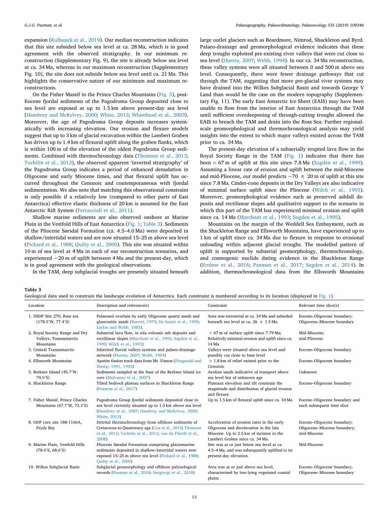
Table 3Geological data used to constrain the landscape evolution of Antarctica. Each constraint is numbered according to its location (displayed in Fig. 1).

Location Description and reference(s) Constraint Relevant time slice(s)

1. DSDP Site 270, Ross sea(178.5°W, 77.4°S)

Palaeosol overlain by early Oligocene quartz sands andglauconitic sands (Barrett, 1975; De Santis et al., 1999;Leckie and Webb, 1983).

Area was terrestrial at ca. 34Ma and subsidedbeneath sea level at ca. 26 ± 1.5Ma.

Eocene–Oligocene boundary;Oligocene–Miocene boundary

2. Royal Society Range and DryValleys, TransantarcticMountains

Subaerial lava flow, in situ volcanic ash deposits andrectilinear slopes (Marchant et al., 1993; Sugden et al.,1999; Wilch et al., 1993)

< 67m of surface uplift since 7.79Ma;Relatively minimal erosion and uplift since ca.14Ma

Mid-Miocene;mid-Pliocene

3. Central TransantarcticMountains

Inherited fluvial valleys systems and palaeo-drainagenetwork (Huerta, 2007; Webb, 1994)

Valleys were situated above sea level andpossibly cut close to base level

Eocene–Oligocene boundary

4. Ellsworth Mountains Apatite fission track data from Mt. Vinson (Fitzgerald andStump, 1991, 1992)

> 1.8 km of relief existed prior to theCenozoic

Eocene–Oligocene boundary

5. Berkner Island (45.7°W,79.5°S)

Sediments sampled at the base of the Berkner Island icecore (Mulvaney et al., 2007)

Aeolian sands indicative of transport abovesea level but of unknown age

Unknown

6. Shackleton Range Tilted bedrock plateau surfaces in Shackleton Range(Paxman et al., 2017)

Plateaux elevation and tilt constrain themagnitude and distribution of glacial erosionand flexure

Eocene–Oligocene boundary

7. Fisher Massif, Prince CharlesMountains (67.7°W, 72.3°S)

Pagodroma Group fjordal sediments deposited close tosea level currently situated up to 1.5 km above sea level(Hambrey et al., 2007; Hambrey and McKelvey, 2000;White, 2013)

Up to 1.5 km of flexural uplift since ca. 34Ma Eocene–Oligocene boundary andeach subsequent time slice

8. ODP core site 188-1166A,Prydz Bay

Detrital thermochronology from offshore sediments ofCretaceous to Quaternary age (Cox et al., 2010; Thomsonet al., 2013; Tochilin et al., 2012; van de Flierdt et al.,2008)

Acceleration of erosion rates in the earlyOligocene and deceleration in the lateMiocene. Up to 2.5 km of incision in theLambert Graben since ca. 34Ma.

Eocene–Oligocene boundary;Oligocene–Miocene boundary;mid-Miocene

9. Marine Plain, Vestfold Hills(78.0°E, 68.6°S)

Pliocene Sørsdal Formation comprising glaciomarinesediments deposited in shallow/intertidal waters nowexposed 15–25m above sea level (Pickard et al., 1988;Quilty et al., 2000)

Site was at or just below sea level at ca.4.5–4Ma, and was subsequently uplifted to itspresent-day elevation.

Mid-Pliocene

10. Wilkes Subglacial Basin Subglacial geomorphology and offshore palynologicalrecords (Paxman et al., 2018; Sangiorgi et al., 2018)

Area was at or just above sea level,characterised by low-lying vegetated coastalplains

Eocene–Oligocene boundary;Oligocene–Miocene boundary

G.J.G. Paxman, et al. Palaeogeography, Palaeoclimatology, Palaeoecology 535 (2019) 109346

13

indicate that at least 1.8 km of relief was present prior to the glaciation(Fitzgerald and Stump, 1992); Mt. Vinson stands ~2 km above the floorof the Rutford trough in our ca. 34Ma reconstruction.

Our erosion estimate shows relatively little incision across largeareas within the interior of East Antarctica such as DML and the GSM(Fig. 5), supporting the findings of earlier ice sheet-erosion modellingstudies (Jamieson et al., 2010). Geomorphological mapping of DML andthe GSM reveals alpine glacial landscapes, which likely formed duringthe early stages of continental glaciation and have remained relativelyunmodified for millions of years (Chang et al., 2015; Creyts et al., 2014;Rose et al., 2013). In these regions, our erosion estimates are indicativeof long-term catchment-averaged erosion rates on the order of10–20m/Myr since at least 34Ma, which are in good agreement withthermochronology data from detrital sediments in Prydz Bay (Fig. 1)(Cox et al., 2010; Tochilin et al., 2012; van de Flierdt et al., 2008).

An ice core from Berkner Island, an ice rise within the Ronne-Filchner Ice Shelf grounded on a shallow seabed plateau in the WeddellSea, revealed that the ice is underlain by well-sorted, quartz-rich sands,which are interpreted as aeolian in origin but of unknown age(Mulvaney et al., 2007). The implication is that Berkner Island wassituated above sea level when these sands were deposited. In ourmedian reconstruction, the ice core location (Fig. 1) was situated100–200m above sea level (under ice-free conditions) since ca. 34Ma.These aeolian sands may therefore have been transported at any timeduring an interval in which the core site was free of ice; without an ageconstraint for the sands, the topographic evolution of Berkner Islandremains unclear.

5.2. Comparison with previous palaeotopography reconstructions

In our median Eocene–Oligocene boundary topography, much ofWest Antarctica is up to 500m lower than the average topography ofWilson et al. (2012) (Supplementary Fig. 12). This is largely because werequired a lower average thickness of eroded material to match con-straints from updated offshore sediment records. We therefore do notproduce such a substantial upland feature in West Antarctica. The totalAntarctic land area above sea level in our median ca. 34Ma re-construction (12.2× 106 km2) is closer to the area in the minimumtopography of Wilson et al. (2012) (12.7× 106 km2) than in theirmaximum topography (13.5× 106 km2). In East Antarctica, we findthat differences in elevation are more subtle and shorter in wavelength(Supplementary Fig. 12). These differences likely reflect the improvedmodern bedrock DEM and offshore sediment thickness maps, both ofwhich yield improved resolution in the reconstructed topographies.

Topographies for ca. 23Ma and ca. 14Ma were previously producedusing a simple linear interpolation between the Wilson et al. (2012)topography and the present-day (Gasson et al., 2016). However, ourmodel accounts for more complex temporal and spatial variability inerosion, sedimentation, thermal subsidence and isostasy. There aretherefore differences between our ca. 23Ma and ca. 14Ma topographiesand those of Gasson et al. (2016). Because thermal subsidence ratesdecay exponentially with time in our models as opposed to linearly asassumed by Gasson et al. (2016), West Antarctica is on average ~300mlower at ca. 23Ma in our scenario than in that of Gasson et al. (2016)(Supplementary Fig. 12). East Antarctic subglacial basins such as Wilkesand Aurora are ~200m lower at ca. 23Ma in our model than in that ofGasson et al. (2016) (Supplementary Fig. 12). By ca. 14Ma, the dif-ferences are more subtle, with the largest differences located around theWeddell Sea, which may in part reflect the increased coverage ofmodern bedrock elevation data in this vicinity (Supplementary Fig. 1).

In a companion paper in this issue, Pollard and DeConto (2019) usea complementary model-based approach, explicitly integrating erosionand sedimentation processes forward in time. This approach producesmaps of simulated past bedrock topography and 3D fields of modernsediment layers that can be compared directly with our results, pro-viding insights into the strengths and uncertainties of both studies.

Preliminary comparisons between the two studies are provided in theSupplementary Material of Pollard and DeConto (2019).

5.3. Implications for Antarctic glacial history

The evolution of Antarctica's subglacial topography raises a numberof implications for the past behaviour of the AIS. The ca. 34Ma topo-graphy has significantly less area below sea level and much shallowermarine basins than the modern topography (Table 2; SupplementaryFig. 8). This implies that the early Antarctic ice sheets would have beenless sensitive to climate and ocean forcing and less vulnerable to rapidand irreversible changes associated with marine ice sheet instability,since areas of reverse-sloping marine bed were less extensive and lesssteep (Fig. 6).

Our findings also have implications for the erosive history of theAIS. The incision of deep troughs transverse to the continental marginin East Antarctica during the Oligocene and early Miocene (Fig. 7) isindicative of a dynamic and erosive EAIS during this interval. After ca.14Ma, erosion/sedimentation rates appear to have decelerated mark-edly (Fig. 7), as is also implied by detrital thermochronology data fromPrydz Bay (Tochilin et al., 2012). This change may have been climati-cally controlled, but may also reflect coastal subglacial troughsreaching a critical depth threshold, whereby the ice sheet was no longerable to avoid flotation, and the rate of erosion decreased. Such a sce-nario has been hypothesised for the Lambert Graben, which has beenoverdeepened to the extent that ice is unable to ground and advanceonto the outer shelf without a significant increase in ice thickness, in-hibiting significant further erosion (Taylor et al., 2004). By contrast,offshore sediment stratigraphic records indicate that West Antarcticawitnessed an increase in erosion rates after the mid-Miocene (Lindequeet al., 2016) (Fig. 7). This may be indicative of the presence of moreerosive, fluctuating ice sheets in West Antarctica after ca. 14Ma.

The contrasting landscape and ice sheet histories of East and WestAntarctica also have implications for marine ice sheet instability,whereby ice sheets grounded on inland-dipping bed below sea level canbe subject to rapid and self-sustained retreat, a process thought to beparticularly pertinent to the modern West Antarctic Ice Sheet (Joughinand Alley, 2011; Mercer, 1978; Vaughan et al., 2011). However, theimplication of the landscape evolution scenario in this study is thatprior to ca. 14Ma, marine ice sheet ice sheet instability was mostpertinent to the East Antarctic margin. After ca. 14Ma, as West Ant-arctica had subsided below sea level and the bed was increasinglyoverdeepened, marine ice sheet instability would have become in-creasingly important in West Antarctica.

These new topographies also have important implications formodelling long-term changes in palaeoclimate, ice sheets, and sea level.Use of relevant palaeotopographies will be important when attemptingquantify variations in Antarctica's ice volume and sea level contribu-tions during past climate transitions at ca. 34, 23, 14, and 3.5Ma, andthereby deconvolve ice volume and ocean temperature contributionsfrom geochemical proxies such as benthic oxygen isotope records.

6. Conclusions

In this study, we have reconstructed Antarctic palaeotopography atfour time intervals since the Eocene–Oligocene boundary (ca. 34Ma).We conclude the following:

1. Our ca. 34Ma topography contains a land area above sea level of12.2× 106 km2, which is ~25% greater than at the present-day.The most significant changes in elevation in East Antarctica haveoccurred within the deep subglacial troughs close to the modern icemargin, some of which have been eroded by> 2 km. The low-lyingWilkes, Aurora and Recovery subglacial basins, which are thought tobe particularly vulnerable to ice sheet retreat, were situated at0–500m above sea level at ca. 34Ma. Much of the WARS was

G.J.G. Paxman, et al. Palaeogeography, Palaeoclimatology, Palaeoecology 535 (2019) 109346

14

situated up to 500m above sea level, and has subsequently de-creased in elevation due to thermal subsidence and glacial erosion.

2. Constraints from offshore sediment records, geomorphology, andgeological datasets indicate that long-term catchment-averagederosion rates are on the order 10–20m/Myr. Erosion rates in EastAntarctica decreased by ~50% after the mid-Miocene (ca. 14Ma),whereas in West Antarctica, erosion rates approximately doubledafter ca. 14Ma. This implies that glaciers around the East Antarcticmargin would have become vulnerable to marine ice sheet in-stability sooner than in West Antarctica.

3. Our new palaeotopographies provide an important boundary con-dition for models seeking to understand past behaviour of theAntarctic Ice Sheet, and the implications for changes in global icevolume, temperature, and sea level across major climate transitionsof the Cenozoic.

Acknowledgements

GJGP is in receipt of a Natural Environment Research Council UKstudentship NE/L002590/1 and was also supported by a RoyalAstronomical Society grant. KH was funded by the German ResearchFoundation (DFG) grant GO274/15 and also acknowledges the tre-mendous help of J. Whittaker, I Sauermilch and the University ofTasmania Visiting Scholar scheme for additional funding during a re-search stay. FF acknowledges support from the British Antarctic SurveyGeology and Geophysics team. We also wish to thank Mikhail Kaban forproviding us with a grid of Antarctic effective elastic thickness. Thisresearch is a contribution to the Scientific Committee on AntarcticResearch (SCAR) Past Antarctic Ice Sheet dynamics (PAIS) programme.We would like to acknowledge the support of numerous members ofSCAR and PAIS and all contributors to the various ANTscape workshopson Antarctic palaeotopography and palaeobathymetry that were in-strumental in the production of the topographies in this paper. We alsothank Peter Barrett and Stuart Thomson for their constructive reviews,which greatly improved the final manuscript. The palaeotopographygrids produced in this study are available online as supplementarymaterial. Grids and figures were produced using the Generic MappingTools (GMT) software package version 5 (Wessel et al., 2013).

Appendix A. Supplementary data

Supplementary data to this article can be found online at https://doi.org/10.1016/j.palaeo.2019.109346.

References

Austermann, J., Pollard, D., Mitrovica, J.X., Moucha, R., Forte, A.M., DeConto, R.M.,Rowley, D.B., Raymo, M.E., 2015. The impact of dynamic topography change onAntarctic ice sheet stability during the mid-Pliocene warm period. Geology 43,927–930. https://doi.org/10.1130/G36988.1.

Barker, Peter F., 1999. Proceedings of the Ocean Drilling program, 178 initial reports. In:Barker, P.F., Camerlenghi, A., Acton, G.D. (Eds.), Proceedings of the Ocean DrillingProgram, Initial Reports, Volume 178, Proceedings of the Ocean Drilling Program.Ocean Drilling Program, pp. 147–158. https://doi.org/10.2973/odp.proc.ir.178.1999.

Barker, P.E., Kennett, J.P. (Eds.), 1988. Proceedings of the Ocean Drilling Program, 113Initial Reports, Proceedings of the Ocean Drilling Program. Ocean Drilling Program,College Station, Texas. https://doi.org/10.2973/odp.proc.ir.113.1988.

Baroni, C., Noti, V., Ciccacci, S., Righini, G., Salvatore, M.C., 2005. Fluvial origin of thevalley system in northern Victoria Land (Antarctica) from quantitative geomorphicanalysis. Geol. Soc. Am. Bull. 117, 212–228. https://doi.org/10.1130/B25529.1.

Barrett, P.J., 1975. Textural characteristics of Cenozoic preglacial and glacial sedimentsat Site 270, Ross Sea, Antarctica. Initial Reports Deep Sea Drill. Proj. Leg 28 (28),757–767.

Barrett, P.J., 1991. The Devonian to Triassic Beacon Supergroup of the TransantarcticMountains and correlatives in other parts of Antarctica. In: Tingey, R.J. (Ed.), TheGeology of Antarctica. Oxford University Press, Oxford, UK, pp. 120–152.

Bingham, R.G., Ferraccioli, F., King, E.C., Larter, R.D., Pritchard, H.D., Smith, A.M.,Vaughan, D.G., 2012. Inland thinning of West Antarctic Ice Sheet steered alongsubglacial rifts. Nature 487, 468–471. https://doi.org/10.1038/nature11292.

Boger, S.D., 2011. Antarctica — before and after Gondwana. Gondwana Res. 19,

335–371. https://doi.org/10.1016/j.gr.2010.09.003.Brenn, G.R., Hansen, S.E., Park, Y., 2017. Variable thermal loading and flexural uplift

along the Transantarctic Mountains, Antarctica. Geology 45, 463–466. https://doi.org/10.1130/G38784.1.

Cande, S.C., Stock, J.M., Müller, R.D., Ishihara, T., 2000. Cenozoic motion between Eastand West Antarctica. Nature 404, 145–150. https://doi.org/10.1038/35004501.

Castelino, J.A., Eagles, G., Jokat, W., 2016. Anomalous bathymetry and palaeobathy-metric models of the Mozambique Basin and Riiser Larsen Sea. Earth and PlanetaryScience Letters 455, 25–37. https://doi.org/10.1016/j.epsl.2016.09.018.

Champagnac, J.D., Molnar, P., Anderson, R.S., Sue, C., Delacou, B., 2007. Quaternaryerosion-induced isostatic rebound in the western Alps. Geology 35, 195–198. https://doi.org/10.1130/G23053A.1.

Chang, M., Jamieson, S.S.R., Bentley, M.J., Stokes, C.R., 2015. The surficial and sub-glacial geomorphology of western Dronning Maud Land, Antarctica. J. Maps 5647,1–12. https://doi.org/10.1080/17445647.2015.1097289.

Chen, B., Haeger, C., Kaban, M.K., Petrunin, A.G., 2018. Variations of the effective elasticthickness reveal tectonic fragmentation of the Antarctic lithosphere. Tectonophysics746, 412–424. https://doi.org/10.1016/j.tecto.2017.06.012.

Colleoni, F., De Santis, L., Montoli, E., Olivo, E., Sorlien, C.C., Bart, P.J., Gasson, E.G.W.,Bergamasco, A., Sauli, C., Wardell, N., Prato, S., 2018. Past continental shelf evolu-tion increased Antarctic ice sheet sensitivity to climatic conditions. Sci. Rep. 8,11323. https://doi.org/10.1038/s41598-018-29718-7.

Cook, C.P., Van De Flierdt, T., Williams, T., Hemming, S.R., Iwai, M., Kobayashi, M.,Jimenez-Espejo, F.J., Escutia, C., González, J.J., Khim, B.K., McKay, R.M., Passchier,S., Bohaty, S.M., Riesselman, C.R., Tauxe, L., Sugisaki, S., Galindo, A.L., Patterson,M.O., Sangiorgi, F., Pierce, E.L., Brinkhuis, H., Klaus, A., Fehr, A., Bendle, J.A.P., Bijl,P.K., Carr, S.A., Dunbar, R.B., Flores, J.A., Hayden, T.G., Katsuki, K., Kong, G.S.,Nakai, M., Olney, M.P., Pekar, S.F., Pross, J., Röhl, U., Sakai, T., Shrivastava, P.K.,Stickley, C.E., Tuo, S., Welsh, K., Yamane, M., 2013. Dynamic behaviour of the EastAntarctic ice sheet during Pliocene warmth. Nat. Geosci. 6, 765–769. https://doi.org/10.1038/ngeo1889.

Cox, S.E., Thomson, S.N., Reiners, P.W., Hemming, S.R., van de Flierdt, T., 2010.Extremely low long-term erosion rates around the Gamburtsev Mountains in interiorEast Antarctica. Geophys. Res. Lett. 37. https://doi.org/10.1029/2010GL045106.

Creyts, T.T., Ferraccioli, F., Bell, R.E., Wolovick, M., Corr, H., Rose, K.C., Frearson, N.,Damaske, D., Jordan, T., Braaten, D., Finn, C., 2014. Freezing of ridges and waternetworks preserves the Gamburtsev Subglacial Mountains for millions of years.Geophys. Res. Lett. 41, 8114–8122. https://doi.org/10.1002/2014GL061491.

Davey, F.J., Granot, R., Cande, S.C., Stock, J.M., Selvans, M., Ferraccioli, F., 2016.Synchronous oceanic spreading and continental rifting in West Antarctica. Geophys.Res. Lett. 43, 6162–6169. https://doi.org/10.1002/2016GL069087.

De Santis, L., Prato, S., Brancolini, G., Lovo, M., Torelli, L., 1999. The Eastern Ross Seacontinental shelf during the Cenozoic: implications for the West Antarctic ice sheetdevelopment. Glob. Planet. Chang. 23, 173–196. https://doi.org/10.1016/S0921-8181(99)00056-9.

Decesari, R.C., Wilson, D.S., Luyendyk, B.P., Faulkner, M., 2007. Cretaceous and tertiaryextension throughout the Ross Sea, Antarctica. In: Cooper, A.K. (Ed.), Antarctica: AKeystone in a Changing World – Online Proceedings of the 10th ISAES. U.S. Geol.Surv. Open File Rep.. https://doi.org/10.3133/of2007-1047.srp098. (2007–1047).

DeConto, R.M., Pollard, D., 2016. Contribution of Antarctica to past and future sea-levelrise. Nature 531, 591–597. https://doi.org/10.1038/nature17145.

Eagles, G., Karlsson, N.B., Ruppel, A., Steinhage, D., Jokat, W., Läufer, A., 2018. Erosionat extended continental margins: insights from new aerogeophysical data in easternDronning Maud Land. Gondwana Res. 63, 105–116. https://doi.org/10.1016/j.gr.2018.05.011.

Elliot, D.H., Fanning, C.M., Hulett, S.R.W., 2015. Age provinces in the Antarctic craton:evidence from detrital zircons in Permian strata from the Beardmore Glacier region,Antarctica. Gondwana Res. 28, 152–164. https://doi.org/10.1016/j.gr.2014.03.013.

Escutia, C., Brinkhuis, H., Klaus, A., 2011. IODP expedition 318: from Greenhouse toicehouse at the Wilkes Land Antarctic Margin. Sci. Drill. 12, 15–23. https://doi.org/10.2204/iodp.sd.12.02.2011.

Ferraccioli, F., Finn, C.A., Jordan, T.A., Bell, R.E., Anderson, L.M., Damaske, D., 2011.East Antarctic rifting triggers uplift of the Gamburtsev Mountains. Nature 479,388–392. https://doi.org/10.1038/nature10566.

Fitzgerald, P.G., Stump, E., 1991. Early cretaceous uplift in the Ellsworth Mountains ofWest Antarctica. Science 254, 92–94.

Fitzgerald, P.G., Stump, E., 1992. Early cretaceous uplift of the Southern Sentinel Range,Ellsworth Mountains, West Antarctica. In: Yoshida, Y., Kaminuma, K., Shiraishi, K.(Eds.), Recent Progress in Antarctic Earth Science - Proceedings of the SixthInternational Symposium on Antarctic Earth Science. Terra Scientific PublishingCompany (TERRAPUB), Tokyo, pp. 331–340.

Fitzgerald, P.G., Stump, E., 1997. Cretaceous and Cenozoic episodic denudation of theTransantarctic Mountains, Antarctica: new constraints from apatite fission trackthermochronology in the Scott Glacier region. J. Geophys. Res. 102, 7747–7765.

Ford, A.B., Barrett, P.J., 1975. Basement rocks of the south-central Ross Sea, Site 270,DSDP Leg 28. Initial Reports Deep Sea Drill. Proj. Leg 28 (28), 861–868.

Fretwell, P., Pritchard, H.D., Vaughan, D.G., Bamber, J.L., Barrand, N.E., Bell, R., Bianchi,C., Bingham, R.G., Blankenship, D.D., Casassa, G., Catania, G., Callens, D., Conway,H., Cook, A.J., Corr, H.F.J., Damaske, D., Damm, V., Ferraccioli, F., Forsberg, R.,Fujita, S., Gim, Y., Gogineni, P., Griggs, J.A., Hindmarsh, R.C.A., Holmlund, P., Holt,J.W., Jacobel, R.W., Jenkins, A., Jokat, W., Jordan, T., King, E.C., Kohler, J., Krabill,W., Riger-Kusk, M., Langley, K.A., Leitchenkov, G., Leuschen, C., Luyendyk, B.P.,Matsuoka, K., Mouginot, J., Nitsche, F.O., Nogi, Y., Nost, O.A., Popov, S.V., Rignot,E., Rippin, D.M., Rivera, A., Roberts, J., Ross, N., Siegert, M.J., Smith, A.M.,Steinhage, D., Studinger, M., Sun, B., Tinto, B.K., Welch, B.C., Wilson, D., Young,D.A., Xiangbin, C., Zirizzotti, A., 2013. Bedmap2: improved ice bed, surface and

G.J.G. Paxman, et al. Palaeogeography, Palaeoclimatology, Palaeoecology 535 (2019) 109346

15

thickness datasets for Antarctica. Cryosph. 7, 375–393. https://doi.org/10.5194/tc-7-375-2013.

Gasson, E., DeConto, R.M., Pollard, D., 2015. Antarctic bedrock topography uncertaintyand ice sheet stability. Geophys. Res. Lett. 42, 5372–5377. https://doi.org/10.1002/2015GL064322.

Gasson, E., DeConto, R.M., Pollard, D., Levy, R.H., 2016. Dynamic Antarctic ice sheetduring the early to mid-Miocene. Proc. Natl. Acad. Sci. 113, 3459–3464. https://doi.org/10.1073/pnas.1516130113.

Gohl, K., 2008. Antarctica's continent-ocean transitions: consequences for tectonic re-constructions. In: Cooper, A.K., Barrett, P.J., Stagg, H.M.J., Storey, B.C., Stump, E.,Wise, W. (Eds.), Antarctica: A Keystone in a Changing World - Online Proceedings ofthe 10th ISAES. The National Academies Press, Washington, D.C., pp. 29–38. https://doi.org/10.3133/of2007-1047.kp04.

Golledge, N.R., Kowalewski, D.E., Naish, T.R., Levy, R.H., Fogwill, C.J., Gasson, E.G.W.,2015. The multi-millennial Antarctic commitment to future sea-level rise. Nature526, 421–425. https://doi.org/10.1038/nature15706.

Goodge, J.W., Fanning, C.M., Fisher, C.M., Vervoort, J.D., 2017. Proterozoic crustalevolution of central East Antarctica: age and isotopic evidence from glacial igneousclasts, and links with Australia and Laurentia. Precambrian Res. 299, 151–176.https://doi.org/10.1016/j.precamres.2017.07.026.

Granot, R., Dyment, J., 2018. Late Cenozoic unification of East and West Antarctica. Nat.Commun. 9, 3189. https://doi.org/10.1038/s41467-018-05270-w.

Hambrey, M.J., McKelvey, B., 2000. Major Neogene fluctuations of the East Antarctic icesheet: stratigraphic evidence from the Lambert Glacier region. Geology 28, 887–890.https://doi.org/10.1130/0091-7613(2000)28<887:MNFOTE>2.0.CO;2.

Hambrey, M.J., Glasser, N., McKelvey, B., Sugden, D., Fink, D., 2007. Cenozoic landscapeevolution of an East Antarctic oasis (Radok Lake area, northern Prince CharlesMountains), and its implications for the glacial and climatic history of Antarctica.Quat. Sci. Rev. 26, 598–626. https://doi.org/10.1016/j.quascirev.2006.11.014.

Hayes, D.E., Frakes, L.A., the Shipboard Scientific Party, 1975. Initial Reports of the DeepSea Drilling Project. Leg 28, 211–334.

Hochmuth, K., Gohl, K., 2019. Seaward growth of Antarctic continental shelves sinceestablishment of a continent-wide ice sheet: patterns and mechanisms. Palaeogeogr.Palaeoclimatol. Palaeoecol. 520, 44–54. https://doi.org/10.1016/j.palaeo.2019.01.025.

Hochmuth, K., Gohl, K., Sauermilch, I., Whittaker, J.M., Leitchenkov, G., De Santis, L.,Olivo, E., Uenzelmann-Neben, G., Davy, B.W., 2018. The Interlinked CenozoicEvolution of Ocean Circulation Patterns and Antarctic Ice Sheets FromPaleobathymetric Grids of the Southern Ocean. AGU Fall Meet. Abstr.

Hochmuth, K., Gohl, K., Sauermilch, I., Whittaker, J.M., Leitchenkov, G., DeSantis, L.,Uenzelmann-Neben, G., Davy, B., 2019. A suite of paleobathymetric grids of theCenozoic Southern Ocean - a key to understanding the interlinked evolution of oceancirculation patterns and Antarctic ice sheets. (in preparation).

Huerta, A.D., 2007. Byrd drainage system; evidence of a Mesozoic West Antarctic plateau.In: Cooper, A.K., Raymond, C.R. (Eds.), Antarctica: A Keystone in a Changing World –Online Proceedings of the 10th ISAES X: USGS Open-File Report 2007-1047. p.Extended Abstract 091, (5 p).

Huang, X., Gohl, K., Jokat, W., 2014. Variability in Cenozoic sedimentation and paleo-water depths of the Weddell Sea basin related to pre-glacial and glacial conditions ofAntarctica. Global and Planetary Change 118, 25–41. https://doi.org/10.1016/j.gloplacha.2014.03.010.

Huang, X., Jokat, W., 2016. Middle Miocene to present sediment transport and deposits inthe Southeastern Weddell Sea, Antarctica. Global and Planetary Change 139,211–225. https://doi.org/10.1016/j.gloplacha.2016.03.002.

Jamieson, S.S.R., Sugden, D.E., Hulton, N.R.J., 2010. The evolution of the subglaciallandscape of Antarctica. Earth Planet. Sci. Lett. 293, 1–27. https://doi.org/10.1016/j.epsl.2010.02.012.

Jamieson, S.S.R., Stokes, C.R., Ross, N., Rippin, D.M., Bingham, R.G., Wilson, D.S.,Margold, M., Bentley, M.J., 2014. The glacial geomorphology of the Antarctic icesheet bed. Antarct. Sci. 26, 724–741. https://doi.org/10.1017/S0954102014000212.

Jamieson, S.S.R., Ross, N., Greenbaum, J.S., Young, D.A., Aitken, A.R.A., Roberts, J.L.,Blankenship, D.D., Bo, S., Siegert, M.J., 2016. An extensive subglacial lake andcanyon system in Princess Elizabeth Land, East Antarctica. Geology 44, 87–90.https://doi.org/10.1130/G37220.1.

Jordan, T.A., Ferraccioli, F., Vaughan, D.G., Holt, J.W., Corr, H., Blankenship, D.D., Diehl,T.M., 2010. Aerogravity evidence for major crustal thinning under the Pine IslandGlacier region (West Antarctica). Bull. Geol. Soc. Am. 122, 714–726. https://doi.org/10.1130/B26417.1.

Joughin, I., Alley, R.B., 2011. Stability of the West Antarctic ice sheet in a warming world.Nat. Geosci. 4, 506–513. https://doi.org/10.1038/ngeo1194.

Krohne, N., Lisker, F., Kleinschmidt, G., Klugel, A., Laufer, A., Estrada, S., Spiegel, C.,2016. The Shackleton Range (East Antarctica): an alien block at the rim ofGondwana? Geol. Mag. 1–24. https://doi.org/10.1017/S0016756816001011.

Kulhanek, D.K., Levy, R.H., Clowes, C.D., Prebble, J.G., Rodelli, D., Jovane, L., Morgans,H.E.G., Kraus, C., Zwingmann, H., Griffith, E.M., Scher, H.D., McKay, R.M., Naish,T.R., 2019. Revised chronostratigraphy of DSDP Site 270 and late Oligocene to earlyMiocene paleoecology of the Ross Sea sector of Antarctica. Glob. Planet. Chang. 178,46–64. https://doi.org/10.1016/j.gloplacha.2019.04.002.

Leckie, R.M., Webb, P.-N., 1983. Late Oligocene-early Miocene glacial record of the RossSea, Antarctica: evidence from DSDP Site 270. Geology 11, 578–582.

LeMasurier, W.E., Landis, C.A., 1996. Mantle-plume activity recorded by low-relief ero-sion surfaces in West Antarctica and New Zealand. Bull. Geol. Soc. Am. 108,1450–1466. https://doi.org/10.1130/0016-7606(1996)108<1450:MPARBL>2.3.CO;2.

LeMasurier, W.E., Thomson, J.W., Baker, P.E., Kyle, P.R., Rowley, P.D., Smellie, J.L.,Verwoerd, W.J. (Eds.), 1990. Volcanoes of the Antarctic Plate and Southern Oceans,

Antarctic Research Series. American Geophysical Union, Washington, D. C. https://doi.org/10.1029/AR048.

Lindeque, A., Gohl, K., Wobbe, F., Uenzelmann-Neben, G., 2016. Preglacial to glacialsediment thickness grids for the Southern Pacific Margin of West Antarctica.Geochem. Geophys. Geosyst. 15, 1009–1020. https://doi.org/10.1002/2016GC006401.

Lisker, F., Läufer, A.L., 2013. The Mesozoic Victoria basin: vanished link betweenAntarctica and Australia. Geology 41, 1043–1046. https://doi.org/10.1130/G33409.1.

Lisker, F., Prenzel, J., Läufer, A.L., Spiegel, C., 2014. Recent thermochronological re-search in Northern Victoria Land, Antarctica. Polarforschung 84, 59–66.

Marchant, D.R., Denton, G.H., Sugden, D.E., Swisher, C.C., 1993. Miocene glacial strati-graphy and landscape evolution of the Western Asgard Range, Antarctica. Geogr.Ann. Ser. A. Phys. Geogr. 75, 303–330. https://doi.org/10.1080/04353676.1993.11880398.

McKenzie, D., 1978. Some remarks on development of sedimentary basins. Earth Planet.Sci. Lett. 40, 25–32. https://doi.org/10.1016/0012-821x(78)90071-7.

Mercer, J.H., 1978. West Antarctic ice sheet and CO2 greenhouse effect: a threat of dis-aster. Nature 271, 321–325. https://doi.org/10.1073/pnas.0703993104.

Molnar, P., England, P., 1990. Late Cenozoic uplift of mountain ranges and global climatechange: chicken or egg? Nature 346, 29–34. https://doi.org/10.1038/346029a0.

Müller, R.D., Seton, M., Zahirovic, S., Williams, S.E., Matthews, K.J., Wright, N.M.,Shephard, G.E., Maloney, K.T., Barnett-Moore, N., Hosseinpour, M., Bower, D.J.,Cannon, J., 2016. Ocean basin evolution and global-scale plate reorganization eventssince Pangea breakup. Annu. Rev. Earth Planet. Sci. 44, 107–138. https://doi.org/10.1146/annurev-earth-060115-012211.

Mulvaney, R., Alemany, O., Possenti, P., 2007. The Berkner Island (Antarctica) ice-coredrilling project. Ann. Glaciol. 47, 115–124. https://doi.org/10.3189/172756407786857758.

Näslund, J.O., 2001. Landscape development in western and central Dronning Maud, EastAntarctica. Antarct. Sci. 13, 302–311.

Paxman, G.J.G., Watts, A.B., Ferraccioli, F., Jordan, T.A., Bell, R.E., Jamieson, S.S.R.,Finn, C.A., 2016. Erosion-driven uplift in the Gamburtsev Subglacial Mountains ofEast Antarctica. Earth Planet. Sci. Lett. 452, 1–14. https://doi.org/10.1016/j.epsl.2016.07.040.

Paxman, G.J.G., Jamieson, S.S.R., Ferraccioli, F., Bentley, M.J., Forsberg, R., Ross, N.,Watts, A.B., Corr, H.F.J., Jordan, T.A., 2017. Uplift and tilting of the ShackletonRange in East Antarctica driven by glacial erosion and normal faulting. J. Geophys.Res. Solid Earth 122, 2390–2408. https://doi.org/10.1002/2016JB013841.

Paxman, G.J.G., Jamieson, S.S.R., Ferraccioli, F., Bentley, M.J., Ross, N., Armadillo, E.,Gasson, E.G.W., Leitchenkov, G., DeConto, R.M., 2018. Bedrock erosion surfacesrecord former East Antarctic Ice Sheet extent. Geophys. Res. Lett. 45, 4114–4123.https://doi.org/10.1029/2018GL077268.

Paxman, G.J.G., Jamieson, S.S.R., Ferraccioli, F., Bentley, M.J., Ross, N., Watts, A.B.,Leitchenkov, G., Armadillo, E., Young, D.A., 2019. The role of lithospheric flexure inthe landscape evolution of the Wilkes Subglacial Basin and Transantarctic Mountains,East Antarctica. J. Geophys. Res. Earth Surf. 124, 812–829. https://doi.org/10.1029/2018JF004705.

Pickard, J., Adamson, D.A., Harwood, D.M., Miller, G.H., Quilty, P.G., Dell, R.K., 1988.Early Pliocene marine sediments, coastline, and climate of East Antarctica. Geology16, 158–161. https://doi.org/10.1130/0091-7613(1988)016<0158:EPMSCA>2.3.CO;2.

Pollard, D., DeConto, R.M., 2019. Continuous simulations over the last 40 million yearswith a coupled Antarctic ice sheet-sediment model. Palaeogeography,Palaeoclimatology, Palaeoecology (this issue).

Quilty, P.G., Lirio, J.M., Jillett, D., 2000. Stratigraphy of the Pliocene sørsdal formation,marine plain, Vestfold hills, east Antarctica. Antarct. Sci. 12. https://doi.org/10.1017/S0954102000000262.

Rignot, E., Mouginot, J., Scheuchl, B., 2011. Ice flow of the Antarctic ice sheet. Science333, 1427–1430. https://doi.org/10.1126/science.1208336.

Rocchi, S., LeMasurier, W.E., Di Vincenzo, G., 2006. Oligocene to Holocene erosion andglacial history in Marie Byrd Land, West Antarctica, inferred from exhumation of theDorrel Rock intrusive complex and from volcano morphologies. Geol. Soc. Am. Bull.118, 991–1005. https://doi.org/10.1130/B25675.1.

Rose, K.C., Ferraccioli, F., Jamieson, S.S.R., Bell, R.E., Corr, H.F.J., Creyts, T.T., Braaten,D., Jordan, T.A., Fretwell, P.T., Damaske, D., 2013. Early East Antarctic ice sheetgrowth recorded in the landscape of the Gamburtsev Subglacial Mountains. EarthPlanet. Sci. Lett. 375, 1–12. https://doi.org/10.1016/j.epsl.2013.03.053.

Rose, K.C., Ross, N., Jordan, T.A., Bingham, R.G., Corr, H.F.J., Ferraccioli, F., Le Brocq,A.M., Rippin, D.M., Siegert, M.J., 2015. Ancient pre-glacial erosion surfaces pre-served beneath the West Antarctic Ice Sheet. Earth Surf. Dyn. 3, 139–152. https://doi.org/10.5194/esurf-3-139-2015.

Sangiorgi, F., Bijl, P.K., Passchier, S., Salzmann, U., Schouten, S., McKay, R., Cody, R.D.,Pross, J., Van De Flierdt, T., Bohaty, S.M., Levy, R., Williams, T., Escutia, C.,Brinkhuis, H., 2018. Southern Ocean warming and Wilkes Land ice sheet retreatduring the mid-Miocene. Nat. Commun. 9, 1–11. https://doi.org/10.1038/s41467-017-02609-7.

Sclater, J.G., Christie, P.A.F., 1980. Continental stretching: an explanation of the Post-Mid-Cretaceous subsidence of the central North Sea Basin. J. Geophys. Res. SolidEarth 85, 3711–3739. https://doi.org/10.1029/JB085iB07p03711.

Shen, W., Wiens, D.A., Stern, T., Anandakrishnan, S., Aster, R.C., Dalziel, I., Hansen, S.,Heeszel, D.S., Huerta, A., Nyblade, A., Wilson, T.J., Winberry, J.P., 2017. Seismicevidence for lithospheric foundering beneath the southern Transantarctic Mountains,Antarctica. Geology 46, 1–4. https://doi.org/10.1130/G39555.1.

Slater, T., Shepherd, A., McMillan, M., Muir, A., Gilbert, L., Hogg, A.E., Konrad, H.,Parrinello, T., 2018. A new digital elevation model of Antarctica derived from

G.J.G. Paxman, et al. Palaeogeography, Palaeoclimatology, Palaeoecology 535 (2019) 109346

16

CryoSat-2 altimetry. Cryosph. 12, 1551–1562. https://doi.org/10.5194/tc-2017-223.Spiegel, C., Lindow, J., Kamp, P.J.J., Meisel, O., Mukasa, S., Lisker, F., Kuhn, G., Gohl, K.,

2016. Tectonomorphic evolution of Marie Byrd Land – implications for Cenozoicrifting activity and onset of West Antarctic glaciation. Glob. Planet. Chang. 145,98–115. https://doi.org/10.1016/j.gloplacha.2016.08.013.

Stern, T.A., Baxter, A.K., Barrett, P.J., 2005. Isostatic rebound due to glacial erosionwithin the Transantarctic Mountains. Geology 33, 221–224. https://doi.org/10.1130/G21068.1.

Straume, E.O., Gaina, C., Medvedev, S., Hochmuth, K., Gohl, K., Whittaker, J.M., AbdulFattah, R., Doornenbal, J.C., Hopper, J.R., 2019. GlobSed: Updated Total SedimentThickness in the World's Oceans. Geochemistry, Geophys. Geosystems. https://doi.org/10.1029/2018GC008115.

Studinger, M., Bell, R.E., Blankenship, D.D., Finn, C.A., Arko, R.A., Morse, D.L., Joughin,I., 2001. Subglacial sediments: a regional geological template for ice flow in WestAntarctica. Geophys. Res. Lett. 28, 3493–3496. https://doi.org/10.1029/2000GL011788.

Stump, E., Sheridan, M.F., Borg, S.G., Sutter, J.F., 1980. Early Miocene subglacial basalts,the East Antarctic ice sheet, and uplift of the transantarctic mountains. Science 207,757–759. https://doi.org/10.1126/science.207.4432.757.

Sugden, D.E., Jamieson, S.S.R., 2018. The pre-glacial landscape of Antarctica. Scott.Geogr. J. 134, 203–223. https://doi.org/10.1080/14702541.2018.1535090.

Sugden, D.E., John, B.S., 1976. Glaciers and Landscape. Edward Arnold, London.Sugden, D.E., Denton, G.H., Marchant, D.R., 1995. Landscape evolution of the dry valleys,

transantarctic mountains: tectonic implications. J. Geophys. Res. 100, 9949–9967.https://doi.org/10.1029/94JB02875.

Sugden, D.E., Summerfield, M.A., Denton, G.H., Wilch, T.I., McIntosh, W.C., Marchant,D.R., Rutford, R.H., 1999. Landscape development in the royal society range,southern Victoria Land, Antarctica: stability since the mid-Miocene. Geomorphology28, 181–200. https://doi.org/10.1016/S0169-555X(98)00108-1.

Sugden, D.E., Fogwill, C.J., Hein, A.S., Stuart, F.M., Kerr, A.R., Kubik, P.W., 2014.Emergence of the Shackleton Range from beneath the Antarctic Ice Sheet due toglacial erosion. Geomorphology 208, 190–199. https://doi.org/10.1016/j.geomorph.2013.12.004.

Sugden, D.E., Hein, A.S., Woodward, J., Marrero, S.M., Rodés, Á., Dunning, S.A., Stuart,F.M., Freeman, S.P.H.T., Winter, K., Westoby, M.J., 2017. The million-year evolutionof the glacial trimline in the southernmost Ellsworth Mountains, Antarctica. EarthPlanet. Sci. Lett. 469, 42–52. https://doi.org/10.1016/j.epsl.2017.04.006.

Tauxe, L., Stickley, C.E., Sugisaki, S., Bijl, P., Bijl, P.K., Bohaty, S.M., Brinkhuis, H.,Escutia, C., Flores, J.A., Houben, A.J.P., Iwai, M., Jiménez-Espejo, F., McKay, R.,Passchier, S., Pross, J., Riesselman, C.R., Rhl, U., Sangiorgi, F., Welsh, K., Klaus, A.,Fehr, A., Bendle, J.A.P., Dunbar, R., Gonzlez, J., Hayden, T., Katsuki, K., Olney, M.P.,Pekar, S.F., Shrivastava, P.K., van de Flierdt, T., Williams, T., Yamane, M., 2012.Chronostratigraphic framework for the IODP Expedition 318 cores from the WilkesLand Margin: Constraints for paleoceanographic reconstruction. Paleoceanography27, 1–19. https://doi.org/10.1029/2012PA002308.

Taylor, J., Siegert, M.J., Payne, A.J., Hambrey, M.J., O'Brien, P.E., Cooper, A.K.,Leitchenkov, G., 2004. Topographic controls on post-Oligocene changes in ice-sheetdynamics, Prydz Bay region, East Antarctica. Geology 32, 197–200. https://doi.org/10.1130/G20275.1.

ten Brink, U.S., Stern, T.A., 1992. Rift flank uplifts and Hinterland Basins: comparison of

the Transantarctic Mountains with the Great Escarpment of southern Africa. J.Geophys. Res. 97, 569–585. https://doi.org/10.1029/91JB02231.

Thomson, S.N., Reiners, P.W., Hemming, S.R., Gehrels, G.E., 2013. The contribution ofglacial erosion to shaping the hidden landscape of East Antarctica. Nat. Geosci. 6,203–207. https://doi.org/10.1038/ngeo1722.

Tochilin, C.J., Reiners, P.W., Thomson, S.N., Gehrels, G.E., Hemming, S.R., Pierce, E.L.,2012. Erosional history of the Prydz Bay sector of East Antarctica from detritalapatite and zircon geo- and thermochronology multidating. Geochem. Geophys.Geosyst. 13, 1–21. https://doi.org/10.1029/2012GC004364.

van de Flierdt, T., Hemming, S.R., Goldstein, S.L., Gehrels, G.E., Cox, S.E., 2008. Evidenceagainst a young volcanic origin of the Gamburtsev Subglacial Mountains, Antarctica.Geophys. Res. Lett. 35, L21303. https://doi.org/10.1029/2008GL035564.

van Wyk de Vries, M., Bingham, R.G., Hein, A.S., 2018. A new volcanic province: aninventory of subglacial volcanoes in West Antarctica. Geol. Soc. Lond. Spec. Publ.461, 231–248. https://doi.org/10.1144/SP461.7.

Vaughan, D.G., Barnes, D.K.A., Fretwell, P.T., Bingham, R.G., 2011. Potential seawaysacross West Antarctica. Geochem. Geophys. Geosyst. 12https://doi.org/10.1029/2011GC003688. (n/a-n/a).

Watts, A.B., 2001. Isostasy and Flexure of the Lithosphere. Cambridge University Press,Cambridge.

Webb, P.-N., 1994. Paleo-drainage systems of East Antarctica and sediment supply toWest Antarctic rift system basins. Terra Antarct. 1, 457–461.

Wessel, P., Smith, W.H.F., Scharroo, R., Luis, J., Wobbe, F., 2013. Generic mapping tools:improved version released. EOS Trans. Am. Geophys. Union 94, 409–410. https://doi.org/10.1002/2013EO450001.

White, D.A., 2013. Cenozoic landscape and ice drainage evolution in the Lambert Glacier-Amery Ice Shelf system. Geol. Soc. Lond. Spec. Publ. 381, 151–165. https://doi.org/10.1144/SP381.15.

Whitehead, J.M., Harwood, D.M., McMinn, A., 2003. Ice-distal Upper Miocene marinestrata from inland Antarctica. Sedimentology 50, 531–552. https://doi.org/10.1046/j.1365-3091.2003.00563.x.

Wilch, T.I., Lux, D.R., Denton, G.H., McIntosh, W.C., 1993. Minimal Pliocene-Pleistoceneuplift of the dry valleys sector of the Transantarctic Mountains: a key parameter inice-sheet reconstructions. Geology 21, 841–844. https://doi.org/10.1130/0091-7613(1993)021<0841:MPPUOT>2.3.CO;2.

Wilson, D.S., Luyendyk, B.P., 2006. Bedrock platforms within the Ross Embayment, WestAntarctica: Hypotheses for ice sheet history, wave erosion, Cenozoic extension, andthermal subsidence. Geochem. Geophys. Geosyst. 7, 1–23. https://doi.org/10.1029/2006GC001294.

Wilson, D.S., Luyendyk, B.P., 2009. West Antarctic paleotopography estimated at theEocene-Oligocene climate transition. Geophys. Res. Lett. 36, L16302. https://doi.org/10.1029/2009GL039297.

Wilson, D.S., Jamieson, S.S.R., Barrett, P.J., Leitchenkov, G., Gohl, K., Larter, R.D., 2012.Antarctic topography at the Eocene-Oligocene boundary. Palaeogeogr.Palaeoclimatol. Palaeoecol. 335–336, 24–34. https://doi.org/10.1016/j.palaeo.2011.05.028.

Wilson, D.S., Pollard, D., DeConto, R.M., Jamieson, S.S.R., Luyendyk, B.P., 2013.Initiation of the West Antarctic Ice Sheet and estimates of total Antarctic ice volumein the earliest Oligocene. Geophys. Res. Lett. 40, 4305–4309. https://doi.org/10.1002/grl.50797.

G.J.G. Paxman, et al. Palaeogeography, Palaeoclimatology, Palaeoecology 535 (2019) 109346

17