3 Isotopic Composition and Accurate Mass

3 Isotopic Composition and Accurate Mass

Learning Objectives

• Isotopes and their effects on mass spectra • Translation of isotopic abundances into mass spectral patterns • Analytical information from isotopic patterns • Nominal and accurate mass of molecules and ions • Mass resolution and its effects on isotopic patterns and mass accuracy • Accurate mass as a tool for determining molecular formulas • Ultra-high resolution – aspects and applications.

In the context of general chemistry we rarely pay attention to the different isotopes of the individual elements involved in a reaction. For instance, the molecular mass of tribromomethane, CHBr3, is usually calculated as 252.73 g mol–1 on the basis of relative atomic mass from the Periodic Table. In mass spectrometry, however, we need to more accurately consider individual isotopes, because mass spectrometry is based upon the separation of ions by mass-to-charge ratio, m/z. [1-3]. Thus, there actually is no signal at m/z 252.73 in the mass spectrum of tribromomethane. Instead, major peaks occur at m/z 250, 252, 254, and 256 accompanied by some minor other ones.

In order to successfully interpret a mass spectrum, one needs to understand iso-topic masses and their relation to the atomic weights, isotopic abundances, and the resulting isotopic patterns, and finally, high-resolution and accurate mass meas-urements. These issues are closely related to each other, offer a wealth of analyti-cal information, and are valid for any type of mass spectrometer and any ioniza-tion method employed.

3.1 Isotopic Classification of the Elements

An element is specified by the number of protons in its nucleus. This equals the atomic number Z of the respective element and determines its place within the pe-riodic table of the elements. The atomic number is given as a subscript preceding the elemental symbol, e.g., 6C in case of carbon. Atoms with nuclei of the same atomic number differing in the number of neutrons are termed isotopes. One iso-tope differs from another isotope of the same element in that it possesses a differ-

J. Gross, Mass Spectrometry© Springer-Verlag Berlin Heidelberg 2011

, 2nd ed., DOI 10.1007/978-3-642-10711-5_3,

68 3 Isotopic Composition and Accurate Mass

ent number of neutrons N, i.e., by the mass number A or nucleon number. The mass number of an isotope is given as a superscript preceding the elemental sym-bol, e.g., 12C. The mass number A is the sum of the total number of protons and neutrons in an atom, molecule, or ion [4].

A = Z + N (3.1)

Note: The mass number must not be confused with the atomic number of an element. For the heavier atoms there can be isotopes of the same mass number belonging to different elements, e.g., the most abundant isotopes of both 18Ar and 20Ca have mass number 40.

3.1.1 Monoisotopic Elements

Among 83 naturally occurring stable elements, 20 elements do exist in the form of only one single naturally occurring stable isotope. Therefore, they are termed monoisotopic elements, i.e., all of their atoms have equal A. Among the monoiso-topic elements, fluorine (19F), sodium (23Na), phosphorus (31P), and iodine (127I) belong to the more prominent examples in organic mass spectrometry. Nonethe-less, there are many more such as beryllium (9Be), aluminum (27Al), manganese (55Mn), cobalt (59Co), arsenic (75As), niobium (93Nb), rhodium (103Rh), cesium (133Cs), and gold (197Au). The monoisotopic elements are also referred to as A or X elements. [5,6] If radioactive isotopes were also taken into account, not a single monoisotopic element would remain.

3.1.2 Di-isotopic Elements

Several elements exist naturally in two isotopes and within the context of mass spectrometry it is useful to deal with them as a class of their own. Nevertheless, the term di-isotopic element is not an official one. These elements can even be sub-classified into those having one isotope that is 1 u heavier than the most abun-dant isotope and those having one isotope that is 2 u heavier than the most abun-dant isotope. The first group has been termed A+1 or X+1 elements, the latter ones have been termed A+2 or X+2 elements, respectively [5,6]. If we do not re-strict our view to the elements typically encountered in organic mass spectrome-try, one should add the class of X–1 elements with one minor isotope of 1 u lower mass than the most abundant one.

Prominent examples of X+1 elements are hydrogen (1H, 2H ≡ D), carbon (12C, 13C), and nitrogen (14N, 15N). Deuterium (D) is of low abundance (0.0115%) and therefore, hydrogen is usually treated as a monoisotopic or as an X element, which is a valid approximation, even if a hundred hydrogens are contained in a molecule.

Among the X+2 elements, chlorine (35Cl, 37Cl) and bromine (79Br, 81Br) are rel-atively common, but copper (63Cu, 65Cu), gallium (69Ga, 71Ga), silver (107Ag, 109Ag), indium (113In, 115In), and antimony (121Sb, 123Sb) also belong to this group.

3.1 Isotopic Classification of the Elements 69

Even though occurring in more than two isotopes, some other elements such as oxygen, sulfur, and silicon, can be dealt with as X+2 elements for practical rea-sons. As long as only a few oxygens are part of a formula, oxygen might even be treated as an X element because of the low abundances of 17O and 18O.

Finally, the elements lithium (6Li, 7Li), boron (10B, 11B), and vanadium (50V, 51V) come along with a lighter isotope of lower abundance than the heavier one and thus, they can be grouped together as X–1 elements.

3.1.3 Polyisotopic Elements

The majority of elements are grouped as polyisotopic elements because they con-sist of three or more isotopes showing a wide variety of isotopic distributions.

3.1.4 Representation of Isotopic Abundances

Isotopic abundances are listed either as their sum being 100% or with the abun-dance of the most abundant isotope normalized to 100%. The latter is used throughout this book because this is consistent with the custom of reporting mass spectra normalized to the base peak (Chap. 1). The isotopic classifications and iso-topic compositions of some common elements are listed below (Table 3.1).

Bar graph representations are much better suited for visualization of isotopic compositions than tables, and in fact they exactly show how such a distribution would appear in a mass spectrum (Fig. 3.1). This appearance coined the term iso-topic pattern.

Fig. 3.1. Isotopic patterns of chlorine, bromine, and xenon. The bar graph representations of the isotopic distributions have the same optical appearance as mass spectra.

Note: Some authors use the term isotopic cluster, which is incorrect, as cluster refers to an associate of more atoms, molecules, or ions of the same species, sometimes associated with one other species, e.g., [Arn]

+•, [(H2O)nH]+, and [I(CsI)n]

– are cluster ions.


Table 3.1. Isotopic classifications and isotopic compositions of some common elements. A complete table is provided in the Appendix. © IUPAC 2001 [7,8]

Classifi-cation

Atomic symbol

Atomic number

Z

Mass number

A

Isotopic composition

Isotopic mass [u]

Relative atomic mass

[u] (X)a H 1 1 100 1.007825 1.00795

2 0.0115 2.014101

X F 9 19 100 18.998403 18.998403

X Na 11 23 100 22.989769 22.989769

X P 15 31 100 30.973762 30.973762

X I 53 127 100 126.904468 126.904468

X+1 C 6 12 100 12.000000b 12.0108 13 1.08 13.003355

X+1 N 7 14 100 14.003074 14.00675 15 0.369 15.000109

(X+2)a O 8 16 100 15.994915 15.9994 17 0.038 16.999132 18 0.205 17.999116

(X+2)a Si 14 28 100 27.976927 28.0855 29 5.0778 28.976495 30 3.3473 29.973770

(X+2)a S 16 32 100 31.972071 32.067

33 0.80 32.971459 34 4.52 33.967867 36 0.02 35.967081

X+2 Cl 17 35 100 34.968853 35.4528 37 31.96 36.965903

X+2 Br 35 79 100 78.918338 79.904

81 97.28 80.916291

X–1 Li 3 6 8.21 6.015122 6.941

7 100 7.016004

X–1 B 5 10 24.8 10.012937 10.812

11 100 11.009306

poly Xe 54 124 0.33 123.905896 131.29 126 0.33 125.904270 128 7.14 127.903530 129 98.33 128.904779 130 15.17 129.903508 131 78.77 130.905082 132 100 131.904154 134 38.82 133.905395 136 32.99 135.907221

a Classification in parentheses ≡ “not in the strict sense”. b Standard of atomic mass scale.


Note: Care has to be taken when comparing isotopic abundances from different sources as they might be compiled using one or the other procedure of normali-zation. Never mix normalization modes in your calculations!

3.1.5 Calculation of Atomic, Molecular, and Ionic Mass

3.1.5.1 Nominal Mass

In order to calculate the approximate mass of a molecule we usually sum up inte-ger masses of the elements encountered, e.g., for CO2 we calculate the mass as 12 u + 2 × 16 u = 44 u. The result of this simple procedure is not particularly pre-cise but provides acceptable values for simple molecules. This is called nominal mass [6].

The nominal mass of an element is defined as the integer mass of its most ab-undant naturally occurring stable isotope [6]. The nominal mass of an element is often equal to the integer mass of the lowest mass isotope of that element, e.g., for H, C, N, O, S, Si, P, F, Cl, Br, I (Table 3.1). The nominal mass of an ion is the sum of the nominal masses of its constituent elements.

Example: To calculate the nominal mass of SnCl2, the masses of 120Sn and 35Cl have to be used, i.e., 120 u + 2 × 35 u = 190 u. While the 35Cl isotope represents the most abundant as well as the lowest mass isotope of chlorine, 120Sn is the most abundant but not the lowest mass isotope of tin which is 112Sn.

Note: When dealing with nominal mass, mass number and nominal mass both have the same numerical value. However, the mass number is dimensionless and must not be confused with nominal mass in units of u.

3.1.5.2 Isotopic Mass

The isotopic mass is the exact mass of an isotope. It is very close to but not equal to the nominal mass of the isotope (Table 3.1). The only exception is the carbon isotope 12C which has an isotopic mass of 12.000000 u. The unified atomic mass [u] is defined as 1/12 of the mass of one atom of nuclide 12C which has been as-signed precisely 12 u, where 1 u = 1.660538 × 10–27 kg [4,6,9,10]. This convention dates back to 1961 [2].

Note: Mass values from dated literature can be ambiguous. Prior to 1961 phy-sicists defined the atomic mass unit [amu] based on 1/16 of the mass of one atom of nuclide 16O. The definition of chemists was based on the relative atomic mass of oxygen which is somewhat higher resulting from the nuclides 17O and 18O contained in natural oxygen [2].


3.1.5.3 Relative Atomic Mass

The relative atomic mass or the atomic weight as it is also often imprecisely termed is calculated as the weighted average of the naturally occurring isotopes of an element [6]. The weighted average Mr is calculated from

∑

∑

=

=

×= i

ii

i

iii

r

A

mAM

1

1

(3.2)

with Ai being the abundances of the isotopes and mi their respective isotopic masses [11]. For this purpose, the abundances can be used in any numerical form or normalization as long as they are used consistently.

Example: The relative atomic mass of chlorine is 35.4528 u. However, there is no atom of this mass. Instead, chlorine is composed of 35Cl (34.968853 u) and 37Cl (36.965903 u) making up 75.78% and 24.22% of the total or having relative abun-dances of 100% and 31.96%, respectively (cf. Table 3.1 and Fig 3.1). According to Eq. 3.2, we can now calculate the relative atomic mass of chlorine Mr = (100 × 34.968853 u + 31.96 × 36.965903 u)/(100 + 31.96) = 35.4528 u.

3.1.5.4 Monoisotopic Mass

The exact mass of the most abundant isotope of an element is termed monoiso-topic mass [6]. The monoisotopic mass of a molecule is the sum of the monoiso-topic masses of the elements in its empirical formula. As mentioned before, the monoisotopic mass is not necessarily the naturally occurring isotope of lowest mass. However, for the common elements in organic mass spectrometry the monoisotopic mass is obtained using the mass of the lowest mass isotope of that element, because this is also the most abundant isotope of the respective element (Chap. 3.1.5.1).

3.1.5.5 Relative Molecular Mass

The relative molecular mass, Mr, or molecular weight is calculated from the rela-tive atomic masses of the elements contributing to the empirical formula [6].

3.1.5.6 Exact Ionic Mass

The exact mass or accurate mass of a positive ion formed by the removal of one or more electrons from a molecule is equal to its monoisotopic mass minus the mass of the electron(s), me [4]. For negative ions, the electron mass (0.000548 u) has to be added accordingly.


Example: The exact mass of the carbon dioxide molecular ion, CO2+•, is calcu-

lated as 12.000000 u + 2 × 15.994915 u – 0.000548 u = 43.989282 u.

3.1.5.7 Role of the Electron Mass When Calculating Exact Mass

The question remains whether the mass of the electron me (5.48 × 10–4 u) has real-ly to been taken into account. This issue was of almost pure academic interest as long as mass spectrometry was limited to mass accuracies of several 10–3 u. As FT-ICR, orbitrap, and even recent oaTOF instruments deliver mass accuracies in the order of < 10–3 u, one should routinely include the electron mass in calcula-tions [12,13]. Here, neglecting the electron mass would cause a systematic error of the size of me, which is unacceptable when mass measurement accuracies in the order of < 10–3 u are to be achieved.

3.1.5.8 Number of Decimal Places When Calculating Exact Mass

The isotopic masses provided in this book are listed with six decimal places corre-sponding to an accuracy of 10–6 u (Tab. 3.1 and Appendix), which is about three orders of magnitude below typical mass errors in mass spectrometry (± 0.001 u).

The number of decimal places one should employ in mass calculations depends on the purpose they are used for. In the m/z range of up to about 500 u, the use of isotopic mass with four decimal places may provide sufficient accuracy. Above that, at least five decimal places are required, because the increasing number of atoms results in an unacceptable multiplication of many small mass errors. The re-sults of those calculations may again be reported with only four decimal places (± 0.0001 u), because this is sufficient for most applications.

3.1.6 Natural Variations in Relative Atomic Mass

The masses of isotopes can be measured with accuracies better than parts per bil-lion (ppb), e.g., m40Ar = 39.9623831235 ± 0.000000005 u. Unfortunately, determi-nations of abundance ratios are less accurate, causing errors of several parts per million (ppm) in relative atomic mass. The real limiting factor, however, comes from the variation of isotopic abundances from natural samples, e.g., in case of lead (Pb) which is the final product of radioactive decay of uranium, the atomic weight varies by 500 ppm depending on the Pb/U ratios in the lead ore [11]. Variations in natural isotopic distributions are also responsible for the varying number of decimal places stated with the relative atomic masses in Table 3.1.

For organic mass spectrometry the case of carbon is of highest relevance. Car-bon is ubiquitous in metabolic processes and the most prominent example of variations in the 13C/12C isotopic ratio is presented by the different pathways of CO2 fixation during photosynthesis, causing 13C/12C ratios of 0.01085–0.01115. Petroleum, coal, and natural gas yield very low 13C/12C ratios of 0.01068–0.01099 and carbonate minerals, on the other side, set the upper limit at about 0.01125


[11]. Even proteins of different origin (plants, fish, mammals) can be distin-guished by their 13C/12C ratios [14,15].

Isotope ratio mass spectrometry (IR-MS) makes use of these facts to determine the origin or the age of a sample. For convenience, the minor changes in isotopic ratios are expressed using the delta notation stating the deviation of the isotopic ratio from a defined standard in parts per thousand (‰) [11,16]. The delta value of carbon, for example, is calculated from

δ13C (‰) = [(13C/12Csample)/(13C/12Cstandard) – 1] × 1000 (3.3)

The internationally accepted value for 13C/12Cstandard is 0.0112372 from a bel-emnite fossil from the Pee Dee formation in South Carolina (PDB standard). Natu-rally occurring 13C/12C ratios range from about δ13C = –50 to +5‰.

As an example, the origin of food can be determined by employing δ13C meas-urements, e.g., fruit/vegetables by country or whether the source of ethanol in al-coholic beverages is sugar cane, sugar beet, cereal starch, or obtained by synthetic processes [14,16,17].

Note: A 13C content of 1.1%, equalling a 13C/12C ratio of 0.0111 has proven to be most useful in the majority of mass spectrometric applications.

3.2 Calculation of Isotopic Distributions

As long as we are dealing with molecular masses in a range of up to some 103 u, it is possible to separate ions which differ by 1 u in mass. The upper mass limit for their separation depends on the resolution of the instrument employed. Conse-quently, the isotopic composition of the analyte is directly reflected in the mass spectrum – it can be regarded as an elemental fingerprint.

Even if the analyte is chemically perfectly pure it represents a mixture of dif-ferent isotopic compositions, provided it is not composed of monoisotopic ele-ments only. Therefore, a mass spectrum normally superimposes the mass spectra of all isotopic species involved [18]. The isotopic distribution or isotopic pattern of molecules containing one chlorine or bromine atom is listed in Table 3.1. But what about molecules containing two or more di-isotopic or even polyisotopic elements? While it may seem, at the first glance, to complicate the interpretation of mass spectra, isotopic patterns are in fact an ideal source of analytical informa-tion.

3.2.1 Carbon: An X+1 Element

In the mass spectrum of methane (Fig. 1.4), there is a tiny peak at m/z 17 that has not been mentioned in the introduction. As one can infer from Table 3.1 this should result from the 13C content of natural carbon which is an X+1 element ac-cording to our classification.

3.2 Calculation of Isotopic Distributions 75

Example: Imagine a total of 1000 CH4 molecules. Due to a content of 1.1% 13C, there will be 11 molecules containing 13C instead of 12C; the remaining 989 molecules are 12CH4. Therefore, the ratio of relative intensities of the peaks at m/z 16 and m/z 17 is defined by the ratio 989/11 or by usual normalization 100/1.1.

In a more general way, carbon consists of 13C and 12C in a ratio r that can be written as r = c/(100 – c) where c is the abundance of 13C. Then, the probability to have only 12C in a molecular ion M consisting of w carbons, i.e., the probability of monoisotopic ions PM is given by [19]

w

McP ⎟

⎠⎞

⎜⎝⎛ −

=100

100

(3.4)

The probability of having exactly one 13C atom in an ion with w carbon atoms is therefore

w

Mc

ccwP ⎟

⎠⎞

⎜⎝⎛ −

⎟⎠⎞

⎜⎝⎛

−=+ 100

1001001

(3.5)

and the ratio PM+1/PM is given as

⎟⎠⎞

⎜⎝⎛

−=+

ccw

PP

M

M

1001

(3.6)

In case of a carbon-only molecule such as the buckminster fullerene C60, the ra-tio PM+1/PM becomes 60 × 1.1/98.9 = 0.667. If the monoisotopic peak at m/z 720 due to 12C60 is regarded as 100%, the M+1 peak due to 12C59

13C will have 66.7% relative intensity.

Note: For the 13C/12C ratio, the M+1 peak intensity can be easily estimated in percent in a simplified manner, and with an insignificant error, by multiplying the number of carbon atoms by 1.1%, e.g., 60 × 1.1% = 66%.

There is again a certain probability for one of the remaining 59 carbon atoms to be 13C rather than 12C. After simplification of Beynon's approach [19] to be used for one atomic species only, the probability that there will be an ion containing two 13C atoms is expressed by

( ) ( )( )2

22

10021

1001

1002 ccww

ccw

ccw

PP

M

M

−

−=⎟

⎠⎞

⎜⎝⎛

−−⎟

⎠⎞

⎜⎝⎛

−=+

(3.6)

For C60 the ratio PM+2/PM now becomes (60 × 59 × 1.12)/(2 × 98.92) = 0.219, i.e., the M+2 peak at m/z 722 due to 12C58

13C2 ions will show as 21.9% relative to the M peak, which definitely can not be neglected. By extension of this principle, equations for the PM+3/PM ratio representing the third isotopic peak can be derived and so forth.


The calculation of isotopic patterns as just shown for the carbon-only molecule C60 can be done analogously for any X+1 element. Furthermore, the application of this scheme is not restricted to molecular ions, but can also be used for fragment ions. Nevertheless, care should be taken to assure that the presumed isotopic peak is not partially or even completely due to a different fragment ion, e.g., an ion con-taining one hydrogen more than the presumed X+1 composition.

Note: It is very helpful to read out the PM+1/PM ratio from a mass spectrum to calculate the approximate number of carbon atoms. Provided no other element contributing to M+1 is present, an M+1 intensity of 15%, for example, indi-cates the presence of 14 carbons. (For possible overestimation due to autopro-tonation cf. Chap. 7.2.1)

Fig. 3.2. Calculated isotopic patterns for carbon. Note the steadily expanding width of the pattern as X+2, X+3, X+4,... become visible. At about C90 the X+1 peak reaches the same intensity as the X peak. At higher carbon numbers it becomes the base peak of the pattern.

It is interesting how the width of the isotopic pattern increases as X+2, X+3, X+4 ... become detectable. In principle, the isotopic pattern of Cw expands up to X+w, because even the composition 13Cw is possible. As a result, the isotopic pat-tern of w atoms of a di-isotopic element consists at least theoretically of w+1 peaks. However, the probability of extreme combinations is negligible and even somewhat more probable combinations are of no importance as long they are be-low about 0.1%. In practice, the interpretation of the carbon isotopic pattern is limited by experimental errors in relative intensities rather than by detection limits for peaks of low intensity. Such experimental errors can be due to poor signal-to-noise ratios (Chap. 1.4.3), autoprotonation (Chap.7), or interference with other peaks.

At about C90 the X+1 peak reaches the same intensity as the X peak, and at higher carbon number w, it becomes the base peak of the pattern, because the probability that an ion contains at least one 13C becomes larger than that for the monoisotopic ion. A further increase in w makes the X+2 signal stronger than the X and X+1 peak and so on. A table with representative carbon isotopic abun-dances is provided in the Appendix.


3.2.2 Terms Related to Isotopic Composition

Molecules and ions of identical elemental composition but differing in isotopic composition are termed isotopic homologs or simply isotopologs. For example, H3C-CH3 and H3C-13CH3 are isotopologs. Molecules and ions of identical isotopic composition but differing in position of the isotopes are termed isotopomers. For example, H2C=CD2 and HDC=CHD are isotopomers.

The isotopic molecular ion (M+1, M+2, ...) is a molecular ion containing one or more of the less abundant naturally occurring isotopes of the atoms that make up the molecular structure [4]. This term can be generalized for any non-monoisotopic ion. Thus, isotopic ions are those ions containing one or more of the less abundant naturally occurring isotopes of the atoms that make up the ion.

The position of the most intensive peak of an isotopic pattern is termed most abundant mass [6], and the corresponding ion should be named most abundant isotopolog (ion). For example, the most abundant mass in case of C120 is 1441 u corresponding to M+1 (Fig. 3.2). The most abundant mass is relevant in the case of large ions (Chap. 3.4.3).

3.2.3 Binomial Approach

The above stepwise treatment of X+1, X+2, and X+3 peaks has the advantage that it can be followed easier, but it bears the disadvantage that an equation needs to be solved for each individual peak. Alternatively, one can calculate the relative abun-dances of the isotopic species for a di-isotopic element from a binomial expression [20-22]. In the term (a + b)n the isotopic abundances of both isotopes are given as a and b, respectively, and n is the number of this species in the molecule.

( ) ( ) ( )( )( ) ( ) ...!3/21

!2/133

221

+−−+

−++=+

−

−−

bannn

bannbnaaban

nnnn

(3.8)

For n = 1 the isotopic distribution can of course be directly obtained from the isotopic abundance table (Table 3.1 and Fig. 3.1) and in case of n = 2, 3, or 4 the expression can easily be solved by simple multiplication, e.g.,

( )( )( ) 4322344

32233

222

464

33

2

babbabaaba

babbaaba

bababa

++++=+

+++=+

++=+

(3.9)

Again, we obtain w+1 terms for the isotopic pattern of w atoms. The binomial approach works for any di-isotopic element, regardless of whether it is of X+1, X+2, or X–1 type. However, as the number of atoms increases above 4 it is also no longer suitable for manual calculations.


3.2.4 Halogens

The halogens Cl and Br occur in two isotopic forms, each of them being of sig-nificant abundance, whereas F and I are monoisotopic (Table 3.1). In most cases there are only a few Cl and/or Br atoms in a molecule and this predestinates the binomial approach for this purpose. For halogens the isotopic peaks are separated by 2 u.

Fig. 3.3. Calculated isotopic patterns for combinations of bromine and chlorine. The peak shown at zero position corresponds to the monoisotopic ion at m/z X. The isotopic peaks are then located at m/z = X+2, 4, 6, ... The numerical value of X is given by the mass num-ber of the monoisotopic combination, e.g., 70 u for Cl2.

Example: The isotopic pattern of Cl2 is calculated from Eq. 3.9 with the abun-dances a = 100 and b = 31.96 as (100 + 31.96)2 = 10,000 + 6392 + 1019. After normalization we obtain 100 : 63.9 : 10.2 as the relative intensities of the three peaks. Any other normalization for the isotopic abundances would give the same result, e.g., a = 0.7578, b = 0.2422. The calculated isotopic pattern of Cl2 can be understood from the following practical consideration: The two isotopes 35Cl and


37Cl can be combined in three different ways: i) 35Cl2 giving rise to the monoiso-topic composition, ii) 35Cl37Cl yielding the first isotopic peak which is here X+2, and finally iii) 37Cl2 giving the second isotopic peak X+4. The combinations with a higher number of chlorine atoms can be explained accordingly.

Note: Rapid estimation of the isotopic patterns of chlorine and bromine can be achieved with good results by using the approximate isotope ratios 35Cl/37Cl = 3 : 1 and 79Br/81Br = 1 : 1. Visual comparison with calculated pat-terns is also suitable (Fig. 3.3).

It is helpful to have frequent isotopic distributions at hand. For some Clx, Bry, and ClxBry combinations these are tabulated in the Appendix. Tables are useful for the construction of isotopic patterns from “building blocks”. Nevertheless, as vis-ual information is easier to compare with a plotted spectrum, these patterns are al-so shown below (Fig. 3.3). In case of Cl and Br the peaks are always separated from each other by 2 u, i.e., the isotopic peaks are located at X+2, 4, 6 and so on.

If there are two bromine or four chlorine atoms contained in the formula, the isotopic peaks become stronger than the monoisotopic peak, because the second isotope is of much higher abundance than in case of the 13C isotope.

Hint: One may want to seek advice on how to distinguish between those pat-terns. For example, the patterns of Cl2Br and Cl3Br or of Cl2Br3 and Cl3Br3 closely resemble each other. To distinguish such pairs it is helpful to construct orientation lines between signal peak tips of comparable intensity. Generally these will de-cline with one pattern but can be positively inclined or even close to horizontal in others (Fig. 3.4).

Fig. 3.4. Aid in distinguishing isotopic patterns by using orientation lines. Left side: pat-terns with four peaks each; right side: patterns with six peaks.


3.2.5 Combinations of Carbon and Halogens

So far we have treated the X+1 and the X+2 elements separately, admittedly a ra-ther artificial approach. The combination of C, H, N, and O with the halogens F, Cl, Br, and I covers a large fraction of the molecules one usually has to deal with. When regarding H, O, and N as X elements, which is a valid approximation for not too large molecules, the construction of isotopic patterns can be conveniently accomplished. By use of the isotopic abundance tables of the elements or of tables of frequent combinations of these as provided in this chapter or in the Appendix, the building blocks can be combined to obtain more complex isotopic patterns.

Example: Let us construct the isotopic pattern of C9N3Cl3 restricting ourselves to the isotopic contributions of C and Cl, i.e., with N as an X element. Here, the isotopic pattern of chlorine can be expected to be dominant over that of carbon. First, from the cubic form of Eq. 3.9 the Cl3 pattern is calculated as follows: (0.7578 + 0.2422)3 = 0.435 + 0.417 + 0.133 + 0.014 and after normalization this becomes 100 : 95.9 : 30.7 : 3.3. Of course, using the tabulated abundances of the Cl3 distribution (Appendix) would be faster. The result is then plotted with 2 u dis-tance, beginning at the nominal mass of the monoisotopic ion, i.e., 9 × 12 u + 3 × 14 u + 3 × 35 u = 255 u. The contribution of C9 to the pattern is mainly at X+1 where we have 9 × 1.1% = 9.9%, whereas its contribution to X+2 (0.4%, Appendix) is negligible in this simple estimation. Finally, the X+1 contri-bution of C9 is placed into the gaps of the Cl3 pattern each with 9.9% relative to the preceding peak of the chlorine isotopic distribution (Fig. 3.5).

Fig. 3.5. The isotopic pattern of C9N3Cl3 as constructed in the example above. The first 13C isotopic peaks are located between the X+2, 4, and 6 peaks of the dominant Cl3 pattern. Ni-trogen is treated as an X element and has been omitted from the peak labels for clarity.


3.2.6 Polynomial Approach

The polynomial approach is the logical expansion of the binomial approach. It is useful for the calculation of isotopic distributions of polyisotopic elements or for formulas composed of several non-monoisotopic elements [21,22]. In general, the isotopic distribution of a molecule can be described by a product of polynominals

( ) ( ) ( ) ............ 321321321 ++++++++++ onm cccbbbaaa (3.10)

where a1, a2, a3 etc. represent the individual isotopes of one element, b1, b2, b3 etc. represent those of another and so on until all elements are included. The expo-nents m, n, o etc. give the number of atoms of these elements as contained in the empirical formula.

Example: The complete isotopic distribution of stearic acid trichloromethyl-ester, C19H35O2Cl3, is obtained from Eq. 3.10 from the polynomial expression

( ) ( ) ( ) ( )33735

2181716

3521

191312 ClClOOOHHCC AAAAAAAAA +++++

with Ax representing the relative abundances of the isotopes involved for each element. The problem with the calculation of isotopic patterns resides in the enormous number of terms obtained for larger molecules. Even for this simple ex-ample, the number of terms would be (2)19 × (2)35 × (3)2 × (2)3 = 1.297 × 1018. The number is dramatically reduced if like terms are combined which describe the same isotopic composition regardless where the isotopes are located in the mole-cule. However, manual calculations are prone to become tedious if not impracti-cal; computer programs now simplify the process [23,24].

Note: Mass spectrometers usually are delivered with the software for calculat-ing isotopic distributions. Such programs are also offered as internet-based or shareware solutions. While such software is freely accessible, it is still neces-sary to obtain a thorough understanding of isotopic patterns as a prerequisite for adequately interpreting mass spectra.

3.2.7 Oxygen, Silicon, and Sulfur

Oxygen, silicon, and sulfur are polyisotopic elements in the strict sense – oxygen as 16O, 17O, and 18O, sulfur as 32S, 33S, 34S, and 36S, and silicon as 28Si, 29Si, and 30Si. The isotopic patterns of sulfur and silicon are by far not as prominent as those of chlorine and bromine, but still important (Fig. 3.6).

17O (0.038%) and 18O (0.205%) are so rare that the occurrence of oxygen usu-ally cannot be detected from the isotopic pattern in routine spectra because the experimental error in relative intensities tends to be larger than the contribution of 18O. Therefore, oxygen is frequently treated as an X type element although X+2 would be a more appropriate but practically rather useless classification. In oligo-


saccharides, for instance, a substantial number of oxygen atoms contribute to the X+2 signal.

Sulfur can be classified as an X+2 element as long as few sulfur atoms are pre-sent in a molecule. However, the 0.8% contributed by 33S to the X+1 is almost comparable to the situation with 13C (1.1% per atom). If the X+1 peak is used for estimating the number of carbons present, then for 33S this would cause an overes-timation of the number of carbon atoms by roughly one carbon per sulfur.

In the case of silicon the 30Si isotope contributes a “mere” 3.4% to the X+2 sig-nal, and 29Si even 5.1% to X+1. So, neglecting 29Si would cause an overestimation of the carbon number by 5 per Si present, which is unacceptable.

Fig. 3.6. Calculated isotopic patterns for combinations of elemental silicon and sulfur. The peak shown at zero position corresponds to the monoisotopic ion at m/z X. The isotopic peaks are then located at m/z X+1, 2, 3, ...

Note: The presence of S and Si in a mass spectrum is best revealed by carefully examining the X+2 intensity: this signal’s intensity will be too high to be caused by the contribution of 13C2 alone, even if the number of carbons has been obtained from X+1 without prior subtraction of the S or Si contribution.

Example: Ethyl propyl thioether, C5H12S: the isotopic pattern of its elemental composition and.the relative contributions of 33S and 13C to the M+1 and of 34S and 13C2 to the M+2 signal.(see Fig. 3.7 and Chap. 6.12). If the M+1 peak resulted from 13C alone, this would rather indicate the presence of 6 carbon atoms, which in turn would imply an M+2 intensity of only 0.1% instead of the actually ob-served 4.6%. Consideration of Si for explaining the isotopic pattern would still fit the M+2 intensity, however with relatively low accuracy, while for M+1 the situa-


tion would be quite different. As 29Si itself demands 5.1% at M+1, there would be no or one carbon maximum allowed to explain the observed M+1 intensity.

Fig. 3.7. Ethyl propyl thioether, C5H12S – calculated isotopic pattern of the molecular ion indicating the respective contributions of 33S and 13C to the M+1 and of 34S and 13C2 to the M+2 signal.

Fig. 3.8. Tetrabutyltin, C16H36Sn – calculated isotopic pattern..


3.2.8 Polyisotopic Elements

The treatment of polyisotopic elements does not require other techniques as far as calculation or construction of isotopic patterns are concerned. However, isotopic patterns can differ largely from what has been considered so far and it is worth mentioning their peculiarities.

Example: Tin (Sn) – the presence or absence of this polyisotopic element can readily be detected from its characteristic isotopic pattern. For tetrabutyltin, C16H36Sn, the lowest mass isotopic composition is 12C16H36

112Sn, 340 u. Regarding the 16 carbon atoms, the 13C isotopic abundance is about 17.5%. This is superim-posed on the isotopic pattern of elemental Sn, which becomes especially obvious at 345 and 347 u (Fig. 3.7). The bars labeled with a tin isotope alone are almost solely due to xSn12C species. Tin neither has an isotope 121Sn nor 123Sn, and there-fore the contributions at 349 and 351 u must be due to 120Sn13C and 122Sn13C, re-spectively.

3.2.9 Practical Aspects of Isotopic Patterns

The recognition of isotopic patterns bears some potential pitfalls. Particularly, if signals from compounds differing by two or four hydrogens are superimposed or if such a superimposition can not a priori be excluded, the observed pattern has to be stepwise carefully checked to avoid misinterpretation of mass spectral data. When isotopically labeled compounds are involved similar care also becomes nec-essary.

Example: 1-Butene (EI spectrum) – Supposing it to be an unknown, the peaks in the m/z 50–57 range could be misinterpreted as a complex isotopic pattern (Fig. 3.9). However, there is no element having a comparable isotopic pattern, and in addition, all elements exhibiting broad isotopic distributions have much higher mass. Instead, the 1-butene molecular ion loses H•, H2, and multiple H2. The peak at m/z 57, of course, results from 13C. Similarly, the peaks at m/z 39 and 41 erro-neously seem to result from the isotopic distribution of iridium, which is not the case however (191Ir and 193Ir); rather, these peaks originate from the formation of an allyl cation, C3H5

+, m/z 41, which fragments further by loss of H2 to form the C3H3

+ ion, m/z 39 (Chap. 6.2.4).


Fig. 3.9. 1-Butene EI mass spectrum. Adapted with permission. © NIST, 2002.

3.2.10 Bookkeeping with Isotopic Patterns in Mass Spectra

Proving the identity of isotopic patterns requires careful comparison with calcu-lated patterns. The mass differences must be consistent with the mass of the pre-sumed neutral losses. In order to hold true, a pattern can only be assigned to sig-nals at or above the mass given by the sum of all contributing atoms.

In calculating the mass differences between peaks from different isotopic pat-terns it is strongly recommended to proceed from the monoisotopic peak of one group to the monoisotopic peak of the next. Accordingly, the mass difference ob-tained also owes to the loss of a monoisotopic fragment. Otherwise, one bears the risk of erroneously omitting or adding hydrogens in a formula.

Example: The EI mass spectrum of tribromomethane is dominated by the bro-mine isotopic distribution (Fig. 3.10). At first, there is no need to wonder why bromoform fragments like it does upon EI (Chap. 6.1.4). Let us simply accept this fragmentation and focus on the isotopic patterns. By referring to Fig. 3.3 one can identify the patterns of Br3, Br2, and Br. As a matter of fact, the molecular ion must contain the full number of bromine atoms (m/z 250, 252, 254, 256).

The primary fragment ion due to Br• loss will then show a Br2 pattern (m/z 171, 173, 175). A mass difference of 79 u is calculated between m/z 250 and m/z 171, owing to 79Br, and thus identifying the process as a loss of Br•. Starting from the CH79Br2

81Br isotopic ion at m/z 252 would yield the same information if 81Br was used for the calculation. Here, 79Br would wrongly indicate loss of H2Br.

Subsequent elimination of HBr leads to CBr+ at m/z 91, 93. Alternatively, the molecular ion can eliminate Br2 to form CHBr+•, m/z 92, 94, overlapping with the m/z 91, 93 doublet, or it may lose CHBr to yield Br2

+•, causing the peaks at m/z


158, 160, 162. The peaks at m/z 79, 81 are due to Br+ and those at m/z 80, 82 result from HBr+• formed by CBr2 loss from the molecular ion.

Fig. 3.10. Tribromomethane EI mass spectrum. Adapted with permission. © NIST, 2002.

3.2.11 Information from Complex Isotopic Patterns

If the isotopic distribution is very broad and/or there are elements encountered that have a lowest mass isotope of very low abundance, recognition of the mono-isotopic peak would become rather uncertain. However, there are ways to cope with that situation.

Example I: The 112Sn isotopic peak of tin compounds can easily be overlooked or simply could be superimposed by background signals (Fig. 3.8). Here, one should identify the 120Sn peak from its unique position within the characteristic pattern before screening the spectrum from peak to peak. For all other elements contained in the respective ions still the lowest mass isotope would be used in cal-culations.

Example II: Ruthenium exhibits a wide isotopic distribution of which the 102Ru isotope can be used as a marker during assignment of mass differences. Moreover, the strong isotopic fingerprint of Ru makes it easily detectable from mass spectra and even compensates for a lack of information resulting from mod-erate mass accuracy (Fig. 3.11).

3.3 Isotopic Enrichment and Isotopic Labeling 87

M+.C85H76N4ORu

calculated experimental

1270.221270.50

rel.

int.

[%]

m/z m/z

Fig. 3.11. Ruthenium carbonyl porphyrin complex – calculated and experimental isotopic pattern (FD-MS, cf. Chap. 8.5.5). The isotopic pattern supports the presumed molecular composition. The labeled peak corresponds to the 102Ru-containing ion. Adapted from Ref. [25] with permission. © IM Publications, 1997.

Note: If the isotopic distribution is broad and/or there are elements encountered that have a lowest mass isotope of very low abundance, it is recommended to base calculations on the most abundant isotope of the respective element.

3.3 Isotopic Enrichment and Isotopic Labeling

3.3.1 Isotopic Enrichment

If the abundance of a particular nuclide is higher than the natural level in an ion, the term isotopically enriched ion is used to describe any ion enriched in the iso-tope [4]. The degree of isotopic enrichment is best determined by MS.

Example: Isotopic enrichment is a standard means to enhance the response of an analyte in nuclear magnetic resonance (NMR). Such measures gain importance if extremely low solubility is combined with a large number of carbons, as is often the case with [60]fullerene compounds [26]. The molecular ion signals, M+•, of C60 with natural isotopic abundance and of 13C-enriched C60 are shown below (Fig. 3.11; for EI-MS of [60]fullerenes cf. Refs. [27-29]). From these mass spec-tra, the 13C enrichment can be determined by use of Eq. 3.2. For C60 of natural iso-topic abundance we obtain MrC60 = 60 × 12.0108 u = 720.65 u. Applying Eq. 3.2 to the isotopically enriched compound yields Mr13C-C60 = (35 × 720 + 65 × 721 + 98 × 722 + 100 × 723 + 99 × 724 + 93 × 725 + ...)u/(35 + 65 + 98 + 100 + 99 + 93


+ ...) = 724.10 u. (Integer mass and intensity values are used here for clarity.) This result is equivalent to an average content of 4.1 13C atoms per [60]fullerene mole-cule which on the average means 3.45 13C atoms more than the natural content of 0.65 13C atoms per molecule.

m/z

100

50

rel.

int.

%

0

C60

720

721

722

720

721

722723

725

728

m/z

100

50

rel.

int.

%

0

13C-enriched C60

Fig. 3.12. [60]Fullerene – comparison of the molecular ion signals, M+•, with natural iso-topic abundance and of 13C-enriched C60. By courtesy of W. Krätschmer, Max Planck Insti-tute for Nuclear Physics, Heidelberg.

3.3.2 Isotopic Labeling

If the abundance of a particular nuclide is higher than the natural level at one or more (specific) positions within an ion, the term isotopically labeled ion is used to describe such an ion. Among other applications, isotopic labeling is used in order to track metabolic pathways, to serve as internal standard for quantitative analysis, or to elucidate fragmentation mechanisms of ions in the gas phase. In mass spec-trometry, the nonradiating isotopes 2H (deuterium, D), 13C, and 18O are preferably employed and thus, a rich methodology to incorporate isotopic labels has been de-veloped [30]. Isotopic labeling is rather a mass spectrometric research tool [31] than mass spectrometry being a tool to control the quality of isotopic labeling. As a result, isotopic labeling is used in many applications; examples are given throughout the book.

3.4 Resolution and Resolving Power

3.4.1 Definitions

So far, we have taken for granted that mass spectra separate isotopic patterns; now we want to quantify this degree of separation. The separation observed in a mass spectrum is termed mass resolution, R, or simply resolution. Mass resolution is given as the smallest difference in m/z (Δm/z) that can be separated for a given signal, i.e., at a given m/z value:

3.4 Resolution and Resolving Power 89

z/m

z/m

m

mR

Δ=

Δ=

(3.11)

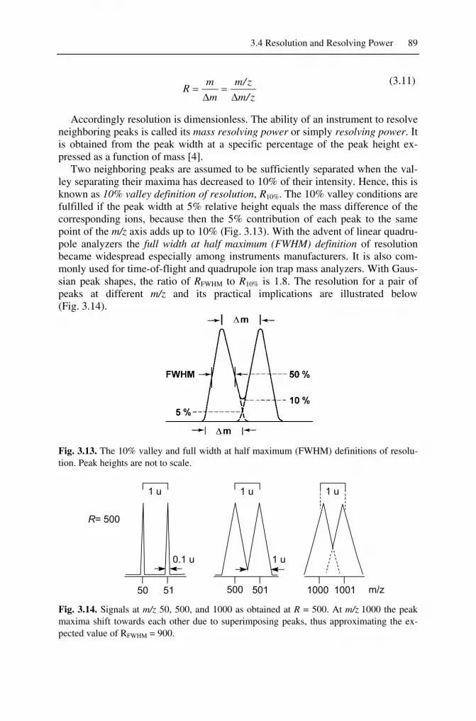
Accordingly resolution is dimensionless. The ability of an instrument to resolve neighboring peaks is called its mass resolving power or simply resolving power. It is obtained from the peak width at a specific percentage of the peak height ex-pressed as a function of mass [4].

Two neighboring peaks are assumed to be sufficiently separated when the val-ley separating their maxima has decreased to 10% of their intensity. Hence, this is known as 10% valley definition of resolution, R10%. The 10% valley conditions are fulfilled if the peak width at 5% relative height equals the mass difference of the corresponding ions, because then the 5% contribution of each peak to the same point of the m/z axis adds up to 10% (Fig. 3.13). With the advent of linear quadru-pole analyzers the full width at half maximum (FWHM) definition of resolution became widespread especially among instruments manufacturers. It is also com-monly used for time-of-flight and quadrupole ion trap mass analyzers. With Gaus-sian peak shapes, the ratio of RFWHM to R10% is 1.8. The resolution for a pair of peaks at different m/z and its practical implications are illustrated below (Fig. 3.14).

Fig. 3.13. The 10% valley and full width at half maximum (FWHM) definitions of resolu-tion. Peak heights are not to scale.

50 51 500 501 1000 1001

0.1 u 1 u

1 u1 u 1 u

R= 500

m/z

Fig. 3.14. Signals at m/z 50, 500, and 1000 as obtained at R = 500. At m/z 1000 the peak maxima shift towards each other due to superimposing peaks, thus approximating the ex-pected value of RFWHM = 900.


28.01

31.99

39.96

28.01

18.01

14.00 43.99

m/z

rel.

int.

[%]

N2

O2

Ar CO2

H2ON2

+.

+.

+.+. +.2+

R = 1000

a

28.006

31.989

39.962

28.006

27.995

18.010

14.003 43.995

m/z

rel.

int.

[%]

N2

O2

Ar CO2

CO

H2ON2

+.

+.

+.+. +.2+

+

R = 7000b

Fig. 3.15. Residual air – EI mass spectra (a) at R = 1000 and (b) at R = 7000. The relative intensities are not affected by different resolution. The decimal digits of the mass labels in-dicate achievable mass accuracies under the respective conditions.

Example: The changes in the electron ionization spectra of residual air nicely show the effect of higher resolution (Fig. 3.15). Setting R = 1000 yields a peak width of 0.028 u for the signal at m/z 28. An increase to R = 7000 perfectly sepa-rates the minor contribution of CO+, m/z 27.995, from the predominating N2

+• at m/z 28.006 (The CO+ ion rather results from fragmenting CO2

+• ions than from carbon monoxide in laboratory air.)

Note: The attributive low resolution (LR) is generally used to describe spectra obtained at R = 500–2000. High resolution (HR) is appropriate for R > 5000. However, there is no exact definition of these terms.

3.4.2 Resolution and its Experimental Determination

In principle, resolution is always determined from the peak width of some signal at a certain relative height and therefore, any peak can serve this purpose. As the exact determination of a peak width is not always easy to perform, certain dou-blets of known Δm are being used.

3.4 Resolution and Resolving Power 91

The minimum resolution to separate CO+ from N2+• is 28/0.011 ≈ 2500. The

doublet from the pyridine molecular ion, C5H5N+•, m/z 79.0422, and from the first

isotopic peak of the benzene molecular ion, 13CC5H6+•, m/z 79.0503, necessitates

R = 9750 to be separated. Finally, the doublet composed of the first isotopic ion of [M–CH3]

+• from xylene, 13CC6H7+, m/z 92.0581, and toluene molecular ion,

C7H8+•, m/z 92.0626, requires R = 20,600 for separation (Fig 3.16).

92.1 92.061 92.0626

92.0581

m/zR = 1000 R = 10.000 R = 20.000

rel.

int.

[%]

0.009 u0.09 u

0.0045 u

Fig. 3.16. The peak at m/z 92 from a mixture of xylene and toluene at different settings of resolution. At R = 10,000 some separation of the lower mass ion can already be presumed from a slight asymmetry of the peak. R = 20,600 is needed to fully separate 13CC6H7

+, m/z 92.0581, from C7H8

+•, m/z 92.0626. The m/z scale is the same for all of the signals.

Note: There is no need to use a more accurate value of m/z than nominal and likewise, there is no use of reporting R = 2522.52 exactly as obtained for the CO+/N2

+• pair. It is fully sufficient to know that setting R = 3000 is sufficient for one specific task or that R = 10,000 is suitable for another.

With magnetic sector instruments a resolving power of up to R = 10,000 can routinely be employed, even R = 15,000. In practice, those instruments are rarely adjusted to resolve beyond R = 10,000, e.g., only when interferences of ions of the same nominal m/z need to be excluded. With an instrument in perfect condition, it is possible to achieve higher resolving power; typically they are specified to de-liver about R ≈ 60,000 (on intensive peaks).

3.4.3 Resolving Power and its Effect on Relative Peak Intensity

Increasing resolution does not affect the relative intensities of the peaks, i.e., the intensity ratios for m/z 28 : 32 : 40 : 44 in the spectrum of air generally remain constant (Fig. 3.15). However, increased settings of resolving power are usually obtained at the cost of transmission of the analyzer, thereby reducing the absolute signal intensity. Accordingly, isotopic patterns are not affected by increasing reso-


lution up to R ≈ 10,000; beyond, there can be changes in isotopic patterns due to the separation of different isotopic species of the same nominal mass (Chap. 3.7).

3.5 Accurate Mass

The section on high resolution (HR) already anticipated accurate mass to a certain extent. In fact, HR and accurate mass measurements are closely related and de-pend on each other, because mass accuracy tends to improve as peak resolution is improved. Nevertheless, they should not be confused, as performing a measure-ment at high resolution alone does not equally imply measuring the accurate mass. High resolution separates adjacent signals, accurate mass can deliver mo-lecular formulas [32-34].

Until the early 1980s, accurate mass measurements were nearly restricted to electron ionization, and for a while, the technique even seemed to become aban-doned. New options available through FT-ICR instrumentation then revived the value of accurate mass measurements. The newly developed orbitrap and a new generation of oaTOF analyzers contributed to an increased demand for accurate mass data. Nowadays, formula elucidation can be performed using any ionization method [35], their widespread application thus demanding a thorough understand-ing of their potential and limitations [33].

3.5.1 Exact Mass and Molecular Formulas

Let us briefly repeat: i) the isotopic mass is also the exact mass of an isotope; ii) the isotopic mass is very close but not equal to the nominal mass of that iso-tope; iii) accordingly, the calculated exact mass of a molecule or of a mono-isotopic ion equals its monoisotopic mass; iv) due to the definition of our mass scale, the isotope 12C represents the only exception from non-integer isotopic mass. As a consequence of these individual non-integer isotopic masses, almost no combination of elements in a molecular or ionic formula has the same calculated exact mass, or simply exact mass as it is often referred to, as any other one [36].

Example: The molecular ions of nitrogen, N2+•, carbon monoxide, CO+•, and

ethene, C2H4+•, have the same nominal mass of 28 u, i.e., they are so-called iso-

baric ions. The isotopic masses of the most abundant isotopes of hydrogen, car-bon, nitrogen, and oxygen are 1.007825 u, 12.000000 u, 14.003074 u, and 15.994915 u, respectively. Thus, the calculated ionic masses are 28.00559 u for N2

+•, 27.99437 u for CO+•, and 28.03075 u for C2H4+•. This means they differ by

several 10–3 u, and none of these isobaric ions has precisely 28.00000 u (Chaps. 3.3.4 and 6.9.6).

Note: Historically, 10–3 u is referred to as 1 millimass unit (mmu). There is still use of mmu in the MS community because of its convenience in dealing with small differences in mass. The mmu is in no way an SI unit.

3.5 Accurate Mass 93

3.5.2 Mass Defect

The deviation of exact mass from nominal mass can be to either side, higher or lower, depending on the isotopes encountered. While the matter itself can be eas-ily understood, existing terminology here is somewhat unfortunate. The term mass defect, mdefect, defined as the difference between integer mass, mnominal, and exact mass, mexact, is used to describe this deviation [6].

mdefect = mnominal – mexact (3.12)

Application of this concept leads to positive and negative mass defects. The hy-drogen atom, for example, has a negative mass defect, mdefectH = –7.825 × 10–3 u. In addition, the association of something being “defective” with certain isotopic masses can be misleading. The mass defect was unveiled by Aston [2,3] who al-ready had discovered 212 of the total 287 stable isotopes.

The term mass deficiency better describes the fact that the exact mass of an iso-tope or a complete molecule is lower than the corresponding nominal mass. In case of 16O, for example, the isotopic mass is 15.994915 u, being 5.085 × 10–3 u deficient as compared to the nominal value (mdefectO = 5.085 × 10–3 u). Most iso-topes are more or less mass deficient with a tendency towards larger mass defect for the heavier isotopes, e.g., M35Cl = 34.96885 u (–3.115 × 10–2 u) and M127I = 129.90447 u (–9.553 × 10–2 u).

Mass–energy equivalence is a key postulate of Einstein’s theory of relativity as expressed by his famous equation E = mc2. It explains the conversion of mass into energy during nucleation, and thus, the increasing mass deficiency of the heavier isotopes caused by their larger nuclear binding energy. The binding energy per nucleon steeply increases along the mass numbers from 2H to its maximum around 56Fe and then decreases again somewhat up to 238U (Fig. 3.17). Translation into isotopic mass reveals that for light elements mass is by some 10–3 u above the no-minal value (1H or 14N) whereas some 10–3 u (19F) to almost 10–1 u (127I) below for heavier elements [34]. This also complies with the fact that the radioactive iso-topes of thorium and uranium have isotopic masses above the nominal value, thus reflecting their comparatively unstable nuclei (Appendix). The numerical values of mass deficiency, however, are merely defined by the “arbitrary” setting of 12C as the standard in the atomic mass scale.


Fig. 3.17. Plot of binding energy per nucleon vs. mass number. Reproduced from Ref. [1] by permission. © John Wiley & Sons, 1992.

Among the elements frequently encountered in mass spectrometry, only H, He, Li, Be, B, and N exhibit isotopic masses larger than their nominal value. Among the isotopes with negative mass defect, 1H is the most important one, because each hydrogen adds 7.825 × 10–3 u. Thereby, it significantly contributes to the mass of larger hydrocarbon molecules [37]. In general, the ubiquitous occurrence of hy-drogen in organic molecules causes most of them to exhibit considerable negative mass defects, which again decreases with the number of mass-deficient isotopes, e.g., from halogens, oxygen, or metals.

Example: Plotting the deviations from nominal mass of different oligomers as a function of nominal mass, one finds only pure carbon molecules (such as fullerenes) to be located on the x-axis. Hydrocarbons, due to their large number of hydrogens, receive roughly 1 u from negative mass defect per 1000 u in molecular mass. Halogenated oligomers, on the other hand, are more or less mass deficient and those oligomers containing some oxygen are located in between (Fig. 3.18).


Fig. 3.18. Deviation from nominal mass for some oligomers as a function of nominal mass. PE: polyethylene, PEG: polyethyleneglycol, PTFE: polytetrafluoroethylene, PVC: poly-vinylchloride.

Note: The use of nominal mass is limited to the low mass range. Above about 500 u the first decimal of isotopic mass can be larger than .5 causing it to be rounded up to 501 u instead of the expected value of 500 u. This will in turn lead to severe misinterpretation of a mass spectrum (Chap. 6).

3.5.3 Mass Accuracy

The absolute mass accuracy, Δm/z, is defined as the difference between measured accurate mass and calculated exact mass:

Δm/z = m/zexperimental – m/zcalculated (3.13)

Instead of stating the absolute mass accuracy in units of u, it can also be given as relative mass accuracy, δm/m, i.e., absolute mass accuracy divided by the mass it is determined for:

δm/m = (Δm/z) / (m/z) (3.14)

The relative mass accuracy, δm/m, is normally given in parts per million (ppm). As mass spectrometers tend to have similar absolute mass accuracies over a comparatively wide range, absolute mass accuracy represents a more meaningful way of stating mass accuracies than the use of ppm.


Note: Parts per million (1 ppm = 10–6) is simply a relative measure as are per-cent (%) or permill (parts per thousand, ‰). In addition, parts per billion (1 ppb = 10–9), and parts per trillion (1 ppt = 10–12) are in use.

Example: A magnetic sector mass spectrometer allows for an absolute mass accuracy of Δm/z = 0.002–0.005 u in scanning mode over a range of about m/z 50–1500. At m/z 1200 an error of Δm/z = 0.003 u corresponds to inconspicuous δm/m = 2.5 ppm, whereas the same error yields 60 ppm at m/z 50, which appears to be unacceptably high.

3.5.4 Accuracy and Precision

The concepts of accuracy and precision can best be illustrated using the analogy to a target where the center represents the true value of some physical quantity [38]. Accuracy describes the deviation of the experimental value from the true value, which normally is rather an accepted reference value than a “true” one in the strict sense. Accuracy is high (A+ in Fig. 3.19) if the values from several measurements are close to the reference value. Accuracy depends on systematic errors of an experiment. Precision describes the deviation within a group of de-terminations and it is high (P+ in Fig. 3.19) if the values from several measure-ments are in close proximity to but not necessarily identical with the reference value. Precision is an expression of random error, e.g., as introduced by noise, variation in injection volumes or times. Repeatability and reproducibility are two aspects of precision. Repeatability is connected to the repetition of the same measurement on the same setup within a short time frame while reproducibility is related to long term stability of a setup and inter-platform or inter-operator effects. Suitable statistical evaluation of a widespread dataset can result in an accurate de-termination of a quantity at the cost of lower precision (P– A?), e.g., root-mean-square deviation (Chap. 3.6.4) [39,40].

P+ A- P+ A+ P- A- P- A?

Fig. 3.19. Precision (P) and accuracy (A), along with seven hits on a target.


3.5.5 Mass Accuracy and the Determination of Molecular Formulas

Assuming infinite mass accuracy, we should be able to identify the molecular formula of any ion merely on the basis of its exact mass – the emphasis is on infi-nite mass accuracy (Chap. 3.5.1). In reality we are dealing with errors in the order of one to several ppm depending on the type of instrument and the mode of its op-eration.

Example: The number of possible even-electron ionic formulas based on an unrestricted selection among the elements C, H, N, and O as a function of relative mass error strongly depends on the m/z value of the ion. Here, the formulas pro-posed for the measured signals from [(arginine)1–5+H]+ cluster ions, m/z 175.1189, 349.2309, 523.3427, 697.4548, and 871.5666 were counted for different relative mass error. While the lowest-mass ion is undoubtedly identified up to 5 ppm, the second ion is only unambiguously identified up to 2 ppm (Fig. 3.20). Allowing sulfur (S0–2) in addition would already result in 18 rather than the 7 hits shown for the [(arginine)3+H]+ ion, m/z 523.3427, at 2 ppm error. Taking also odd-electron ions into account would contribute another 15 compositions to this selection. In case of the [(arginine)5+H]+ ion, m/z 871.5666, the number of C, H, N, O hits rea-ches 26 at 1 ppm error and even 232 at 10 ppm.

Fig. 3.20. Number of possible even-electron ionic formulas based on a free selection among the elements C, H, N, O as a function of relative mass error vs. m/z. The data points corre-spond to [(arginine)1–5+H]+ cluster ions, m/z 175.1189, 349.2309, 523.3427, 697.4548, and 871.5666. The lines are meant as visual guides.

Unequivocal formula assignment by accurate mass alone only works in a range up to about m/z 500 depending on the particular restrictions [41]. Obviously, for ions of larger m/z the number of hits rapidly increases beyond a reasonable limit. Even at a high mass accuracy of 1 ppm and with the particular case of peptides the elemental composition can only be unambiguously identified up to about 800 u


[42-44]. Determining the formula of a peptide among all natural peptide composi-tions possible at m/z 1005.4433 requires δm/m = 0.1 ppm [45].

The situation becomes more complicated as more elements and fewer limita-tions of their number must be taken into account. In practice, one must try to re-strict oneself to certain elements and a maximum and/or minimum number of cer-tain isotopes to assure a high degree of confidence in the assignment of formulas. Isotopic patterns provide a prime source of such additional information. Combin-ing the information from accurate mass data and experimental peak intensities with calculated isotopic patterns allows to significantly reduce the number of po-tential elemental compositions of a particular ion [46,47].

3.5.6 Extreme Mass Accuracy – Special Considerations

Even when we have determined a molecular formula, it does not tell us much about the structure of the molecule. According to the mass–energy equivalence (1 u = 931.5 MeV), a mass accuracy of 1 ppm (δm/m = 10–6) roughly corresponds to an energy of 100 keV if an ion of m/z 100 is considered. A mass accuracy of 1 ppb (δm/m = 10–9) still corresponds to an energy of 100 eV, and thus, 1 ppt (δm/m = 10–12) would be required to approach energy differences of 0.1 eV, i.e., between isomers. Obviously, isomers are (almost) perfect isobars [48]. Nonethe-less, it is worth noting that physicist are approaching 10 ppt, at least in the case of single atomic species (Fig. 3.21).

Fig. 3.21. Relative mass uncertainty δm/m for 28Si as a function of time. The most accurate mass of 28Si so far is m(28Si) = 27.876 926 534 96(62) u corresponding to an uncertainty of 0.2 ppt. The dashed line serves as a visual orientation and reveals an improvement in accu-racy by about one order of magnitude per decade. By courtesy of H.-J. Kluge, GSI Helm-holtz Centre for Heavy Ion Research GmbH, Darmstadt, Germany.

3.6 Applied High-Resolution Mass Spectrometry 99

3.6 Applied High-Resolution Mass Spectrometry

Generally, high-resolution mass spectrometry (HR-MS) aims to achieve both high mass resolution and high mass accuracy. These quantities have been introduced without considering the means by which they can be measured. The key to this problem is mass calibration. Resolution alone can separate ions with m/z in close proximity, but it does not automatically reveal where on the m/z axis the respec-tive signals are located. This section deals with the techniques for establishing ac-curate mass data and their analytical evaluation [32,33].

3.6.1 External Mass Calibration

All mass spectrometers require mass calibration before they are put to use. How-ever, proper procedures and the number of required calibration points may largely differ between different types of mass analyzers. Typically, this necessitates sev-eral peaks of well-known m/z values evenly distributed over the mass range of in-terest. These are supplied from a well-known mass calibration compound or mass reference compound. Calibration is then performed by recording a mass spectrum of the calibration compound and subsequent correlation of experimental m/z val-ues to the mass reference list [33,49,50]. Usually, this conversion of the mass ref-erence list to a calibration is accomplished by the mass spectrometer’s software. Thus, the mass spectrum is recalibrated by interpolation of the m/z scale between the assigned calibration peaks to obtain the best match. The mass calibration ob-tained may then be stored in a calibration file and used for future measurements without the presence of a calibration compound. This procedure is termed external mass calibration.

Note: The numerous ionization methods and mass analyzers in use have cre-ated a demand for a large number of calibration compounds to suit their spe-cific needs. Therefore, mass calibration will variously be addressed at the end of the chapters on ionization methods. It is also not possible to specify a general level of mass accuracy with external calibration. Depending on the type of mass analyzer and on the frequency of recalibration, mass accuracy can vary from mediocre 0.5 u to perfect 10–3 u.

Example: Perfluorokerosene (PFK) is a well-established mass calibration standard in EI-MS. It provides evenly spaced CxFy

+ fragment ions over a wide range (Figs. 3.22 and 3.23). The major ions are all mass deficient, with CHF2

+, m/z 51.0046, being the only exception. PFK mixtures are available from low-boiling to high-boiling grades which may be used up to m/z 700–1100. Apart from the highest boiling grades, PFK is suitable to be introduced by the reference inlet (Chap. 5.2.1), a property making it attractive for internal calibration as well. Per-fluorotributylamine, PFTBA (more often termed FC-43) is another frequently used calibrant, a pure compound delivering peaks up to m/z 614 in EI spectra [40,50].


m/z

PFK

rela

t ive

inte

nsity

[%]

Fig. 3.22. Perfluorokerosene, PFK: partial 70-eV EI mass spectrum. The peaks are evenly distributed over a wide m/z range. Also, peaks from residual air occur in the low m/z range.

Fig. 3.23. Reproduction of a partial PFK calibration table (m/z 1–305 range) of a magnetic sector instrument. In order to expand the PFK reference peak list to the low m/z range, 1H, 4He, and peaks from residual air are included, but for intensity reasons 1H, 4He, and CO2 have not been assigned in this particular case.


3.6.2 Internal Mass Calibration

Elemental compositions are preferably assigned via internal mass calibration. The calibration compound can be introduced from a second inlet system or be mixed with the analyte prior to analysis. Mixing calibration compounds with the analyte requires some operational skills in order for it not to modify the analyte or to be modified itself. Therefore, a separate inlet for introducing the calibration com-pound is preferred. This can be done by introducing volatile standards such as PFK from a reference inlet system in electron ionization, by use of a dual-target probe in fast atom bombardment, or by use of a second sprayer in electrospray io-nization.

Internal mass calibration typically affords mass accuracies in the order of 0.1–0.5 ppm with FT-ICR, 0.5–1 ppm with orbitrap, 0.5–5 ppm with magnetic sector, and 1–10 ppm with time-of-flight analyzers. Mass accuracy strongly depends on various parameters such as resolving power, scan rate, scanning method, signal-to-noise ratio of the peaks, peak shapes, overlap of isotopic peaks at same nominal mass, mass difference between adjacent reference peaks etc. The experimentally determined accurate mass should be within a reasonable error range independent of the ionization method and the instrument used [51]. The correct (expected) composition is not necessarily the one with the least error.

Note: Mass accuracy may suffer from too high settings of resolving power if this causes noisy peaks. Often centroids are determined more accurately from smooth and symmetrically shaped peaks at moderate HR. One should be aware of the fact that the position of a peak of 0.1 u width, for example, has to be de-termined to 1/50 of its width to obtain 0.002 u accuracy [32].

Example: For zirconium complexes the molecular ion range of an HR-EI spec-trum is typified by the isotopic pattern of zirconium and chlorine (Fig. 3.24). 90Zr represents the most abundant zirconium isotope which is accompanied by 91Zr, 92Zr, 94Zr, and 96Zr, all of them having considerable abundances. If the peak at m/z 414.9223 represents the monoisotopic ion, then the elemental composition containing 90Zr and 35Cl is the only correct interpretation. Thus, the formula C16H14NCl3Zr can be identified from the composition list (Fig. 3.25). Next, the X+2 and X+4 compositions should mainly be due to 35Cl2

37Cl and 35Cl37Cl2, re-spectively, leading to their identification. All formulas must have a remainder of C16H14N in common. In this example, R = 8000 is the minimum to separate the PFK reference peak at m/z 417 from that of the analyte. Otherwise, the mass as-signment would have been wrong because the peak at m/z 417 would then be cen-tered at a weighted mass average of its two contributors. Alternatively, such a peak may be omitted from both reference list and composition list.


Fig. 3.24. Partial high-resolution EI mass spectrum in the molecular ion region of a zirco-nium complex. At R = 8000 the PFK ion can barely be separated from the slightly more mass-deficient analyte ion. By courtesy of M. Enders, Heidelberg University.

Fig. 3.25. Suggested elemental compositions of the Zr complex shown in Fig. 3.24. The er-ror for each proposal is listed in units of ppm and mmu (0.001 u). U.S. = “unsaturation”, i.e., the number of rings and/or double bonds (Chap. 6.4.4). Here the correct assignments are highlighted with an arrow. By courtesy of M. Enders, Heidelberg University.

Basic Rules: The assignment of molecular formulas from accurate mass • must always be in accordance with the experimentally observed and the calculated isotopic pattern for the assumed composition, • the formula has to obey the nitrogen rule (Chap. 6.2.7), • depending on the ionization method, even-electron or odd-electron ions may be formed exclusively, and thus can rule out some compositions, and • formulas in contradiction to one of these points are erroneous.


3.6.3 Compiling Mass Reference Lists

A reference list may be compiled once the mass spectrum of a calibration standard is known and the elemental composition of the ions that are to be included in the mass reference list are established by an independent measurement,.For this pur-pose, the listed reference masses should be calculated using six decimal digits. Otherwise, one runs a chance of obtaining erroneous reference values, especially when masses of ion series are calculated by multiplication of a subunit. This can easily be done using conventional spreadsheet applications.

Example: Cesium iodide is frequently used for mass calibration in fast atom bombardment (FAB) mass spectrometry (Chap. 10) because it yields cluster ions of the general formula [Cs(CsI)n]

+ in positive-ion and [I(CsI)n]– in negative-ion

mode. For the [Cs(CsI)10]+ cluster ion, m/z 2730.9 is calculated instead of the cor-

rect value m/z 2731.00405 by applying only one decimal digit rather than the exact values M133Cs = 132.905447 and M127I = 126.904468. The error of 0.104 u is ac-ceptable for LR work, but definitely unacceptable if accurate mass measurements are needed.

Fig. 3.26. Chloroform – Printout of elemental compositions of [M–Cl]+ ions as obtained from three subsequent measurements (70 eV EI, R = 8000). The error for each proposal is listed in units of ppm and “mmu”. U.S. (“unsaturation”) is the number of rings and/or dou-ble bonds (Chap. 6.4.4).


3.6.4 Specification of Mass Accuracy

Measured accurate masses, when used to assign molecular formulas, should al-ways be accompanied by their mass accuracies. [52]. Ideally, this can be done by giving the mean mass value and the corresponding error in terms of standard de-viation through several repeated measurements of the same ion. [40] This is defi-nitely not identical to the error usually provided with a mass spectrometer’s soft-ware, where the error is based on the difference of a single pair of calculated and measured values. The reduction of the average mass error goes with the square root of the number of determinations (Chap. 3.5.4) [39].

Example: The [M-Cl]+ ion, [CHCl2]+, represents the base peak in the EI spec-

trum of chloroform. The results of three subsequent determinations for the major peaks of the isotopic pattern are listed below (Fig. 3.26). The typical printout of a mass spectrometer’s data system provides experimental accurate mass and relative intensity of the signal along with absolute and relative mass error as calculated for a set of suggested formulas. Here, the experimentally accurate mass values yield a root-mean-square of 82.9442 ± 0.0006 u for the [12CH35Cl2]

+ ion. The compara-tively small standard deviation of 0.0006 u corresponds to a relative error of 7.5 ppm.

3.6.5 Deltamass

The term deltamass has been coined to define the mass value following the deci-mal point [53] thereby elegantly circumventing the somewhat unfortunate termi-nology related to the mass defect. The deltamass concept is only valid in the con-text for which it has been developed, i.e., to describe mass deviations of peptides from average values. Beyond this context, ambiguities arise from its rigorous ap-plication because i) a mass defect would then be expressed the same way as larger values of negative mass defect, e.g., in case of 127I+ as 0.9045 u and in case of C54H110

+• as 0.8608 u, respectively, and ii) deviations of more than 1 u would be expressed by the same numerical value as those of less than 1 u.

Example: The magnitude of mass defect can provide an idea of what com-pound class is being analyzed (Chap. 3.5.2). At a sufficient level of sophistication, mass defect can even reveal more detail [43]. Peptides consist of amino acids and therefore, their elemental compositions are rather similar independent of their size or sequence. This results in a characteristic relationship of formulas and deltamass values. Phosphorylation and more pronounced glycosylation cause lower del-tamass, because they introduce mass-deficient atoms (P, O) into the molecule. The large number of hydrogens associated with lipidation, on the other side, contrib-utes to a deltamass above normal level. On the average, an unmodified peptide of 1968 u, for example, shows a deltamass of 0.99 u, whereas a glycosylated peptide of the same nominal mass will have a value of 0.76 u. Thus, the deltamass can be employed to obtain information on the type of covalent protein modification [53].


3.6.6 Kendrick Mass Scale

The intention of the Kendrick mass scale is to provide data reduction in a way that homologs can be recognzed by their identical Kendrick mass defect (KMD). Due to the steadily increasing resolution and mass accuracy of modern instrumentation this issue is again gaining importance for complex mixture analysis by MS. The Kendrick mass scale is based on the definition M(CH2) = 14.0000 u [54]. The con-version factor from the IUPAC mass scale, mIUPAC, to the Kendrick mass scale, mKendrick, is therefore 14.000000/14.015650 = 0.9988834:

mKendrick = 0.9988834 mIUPAC (3.15)

Next, we define the Kendrick mass defect, mdefectKendrick, as

mdefectKendrick = mnomKendrick – mKendrick = KMD (3.16)

where mnomKendrick is the nominal Kendrick mass, the closest integer to Kendrick mass (cf. example next page).

Fig. 3.27. Kendrick mass defect vs. nominal Kendrick mass for odd-mass 12Cx ions ([M–H]– ions). The compound classes (O, O2, O3S, and O4S) and the different numbers of rings plus double bonds (Chap. 6.4.4) are separated vertically. Horizontally, the points are spaced by CH2 groups along a homologous series [55]. By courtesy of A.G. Marshall, NHFL, Tal-lahassee.


Example: The IUPAC mass of [C30H49O3]– is 457.3687 u. The Kendrick mass

of this ion is calculated as 457.3687 u × 0.9988834 = 456.8580 u. From this it fol-lows that mnomKendrick = 457 u. The Kendrick mass defect of this ion is thus ob-tained as mdefectKendrick = 457 u – 456.8580 u = 0.1419 u.

To translate spectral data into a useful Kendrick mass plot, a high-resolution mass spectrum is broken into segments of 1 u, which are aligned on the abscissa. Then, the Kendrick mass defect of the isobaric ions contained in the respective segment is plotted onto the ordinate. The resulting graph preserves not only the “coarse” spacing, e.g., about 1 u between odd and even mass values, but also the “fine structure”, i.e., different Kendrick mass defects (KMDs) for different ele-mental compositions across each segment. Homologs are now easily recognized as horizontal rows in the plot [55].

Example: Crude oil / diesel fuel – In a Kendrick plot the composition of com-plex systems can be conveniently displayed. Several thousand elemental composi-tions in the ultra-high resolution spectrum of petroleum crude oil [55] or diesel fuel [56] may be resolved. Such samples consist of numerous compound classes and/or alkylation series with some 30 homologs each that can be visually identi-fied (Fig. 3.27). The formula employed for the preceding example is marked in the plot by an arrow.

3.6.7 Van Krevelen Diagrams

There is yet another tool for the display of composition characteristics of complex mixtures, the van Krevelen diagram [57]. The van Krevelen diagram is a plot of the atomic H/C ratio against the atomic O/C ratio. This plot causes the products related by reactions such as decarboxylation, dehydration, dehydrogenation, or oxidation to be displayed along straight lines. Along with KMD plots, the van Krevelen plot is therefore a major tool for the assessment of complex organic mix-tures such as crude oil and its refinery products or the wide field of natural or-ganic matter (NOM) that represents the largest share of biomass on earth [58-62].

Example: Deep-sea dissolved organic matter (DOM) – The van Krevelen dia-grams show a group of molecules having low H/C (< 0.9) and low O/C (< 0.25) ratios clearly separated from each other (Fig. 3.28) [61]. An enlarged view of this group shows that it comprises 224 different molecular formulas corresponding to molecules that contain up to 35 rings and/or double bonds (r+d, Chap. 6.4.4). Ho-mologous series can be identified along straight lines. Still this does not tell the complete structure of those molecules, but it delivers much more insight into the composition of DOM than pure accurate mass data alone.

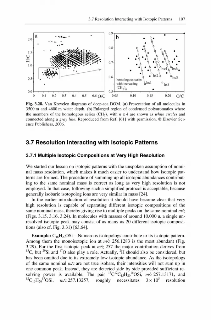
3.7 Resolution Interacting with Isotopic Patterns 107

Fig. 3.28. Van Krevelen diagrams of deep-sea DOM. (a) Presentation of all molecules in 3500 m and 4600 m water depth. (b) Enlarged region of condensed polyaromatics where the members of the homologous series (CH2)n with n ≥ 4 are shown as white circles and connected along a gray line. Reproduced from Ref. [61] with permission. © Elsevier Sci-ence Publishers, 2006.

3.7 Resolution Interacting with Isotopic Patterns

3.7.1 Multiple Isotopic Compositions at Very High Resolution

We started our lesson on isotopic patterns with the unspoken assumption of nomi-nal mass resolution, which makes it much easier to understand how isotopic pat-terns are formed. The procedure of summing up all isotopic abundances contribut-ing to the same nominal mass is correct as long as very high resolution is not employed. In that case, following such a simplified protocol is acceptable, because generally isobaric isotopolog ions are very similar in mass [24].

In the earlier introduction of resolution it should have become clear that very high resolution is capable of separating different isotopic compositions of the same nominal mass, thereby giving rise to multiple peaks on the same nominal m/z (Figs. 3.15, 3.16, 3.24). In molecules with masses of around 10,000 u, a single un-resolved isotopic peak may consist of as many as 20 different isotopic composi-tions (also cf. Fig. 3.31) [63,64].

Example: C16H20OSi – Numerous isotopologs contribute to its isotopic pattern. Among them the monoisotopic ion at m/z 256.1283 is the most abundant (Fig. 3.29). For the first isotopic peak at m/z 257 the major contribution derives from 13C, but 29Si and 17O also play a role. Actually, 2H should also be considered, but has been omitted due to its extremely low isotopic abundance. As the isotopologs of the same nominal m/z are not true isobars, their intensities will not sum up in one common peak. Instead, they are detected side by side provided sufficient re-solving power is available. The pair 13C12C15H20

16OSi, m/z 257.13171, and 12C16H20

17OSi, m/z 257.13257, roughly necessitates 3 × 105 resolution


(R = 257/0.00086 = 299,000). There are six different compositions contributing to the second isotopic peak at m/z 258 and even eight for the third isotopic peak at m/z 259. Again, it is the merit of FT-ICR-MS that resolutions in the order of sev-eral 105 are now available although ultrahigh resolution, as this is termed, is still not fully routine on those instruments (Chap. 4).

Fig. 3.29. C16H20OSi – Tabular representation of the theoretical isotopic distribution at in-finite resolution. The contribution of 2H is not considered, and isotopic peaks above m/z 260 are omitted due to their minor intensities.

Example: Peptides often contain sulfur from cysteine. Provided there are at least two cysteines in the peptide molecule, sulfur can be in the form of thiol group (SH, reduced) or sulfur bridges (S–S, oxidized). Often, both forms are con-tained in the same sample. At ultrahigh resolution, the contributions of these com-positions to the same nominal m/z can be distinguished. The ultrahigh-resolution matrix-assisted laser desorption/ionization (MALDI) FT-ICR mass spectrum of native and reduced [D-Pen2,5]enkephalin is an example of such a separation (Fig. 3.30) [65]. The left expanded view shows fully resolved peaks due to 34S and 13C2 isotopomers of the native and the all-12C peak of the reduced compound at m/z 648. The right expansion reveals the 13C1

34S peak of the native plus the 13C1 signal of the reduced form at m/z 649. Here, RFWHM is more than 9 × 105.


Fig. 3.30. [D-Pen2,5]Enkephalin – Ultrahigh-resolution MALDI-FT-ICR mass spectrum of native (S–S) and reduced (2 × SH).forms. The expanded m/z views of the second and third isotopic peak show fully mass-resolved signals. Reproduced from Ref. [65] with permis-sion. © American Chemical Society, 1997.

Fig. 3.31. Arg8 vasopressin – Theoretical effect of resolution on the shape of the M+2 peak at m/z 1086.4. Theoretical mass spectra of the [vasopressin+H]+ ion and the five indicated resolution values (FWHM) have been superimposed and the bar spectrum corresponds to infinite resolution. Adapted from Ref. [64] with permission. © John Wiley and Sons Ltd., 1994.


3.7.2 Isotopologs and Accurate Mass

It has been pointed out that routine accurate mass measurements are conducted at resolutions which are normally too low to separate isobaric isotopologs. Unfortu-nately, multiple isotopic compositions under the same signal tend to distort the peak shape (Fig. 3.31) [64]. This effect causes problems when elemental composi-tions have to be determined from such multi-isotopolog peaks, e.g., if the monoisotopic peak is too weak as in case of many transition metals. Generally, the ob-served decrease in mass accuracy is not dramatic and is somewhat counterbal-anced by the information derived from the isotopic pattern. However, it can be ob-served that mass accuracy decreases by about 50% on such unresolved signals.

If isotopolog ions are resolved or if certain isotopologs are free from interfer-ence, and provided sufficient mass accuracy is available, the distance between iso-topic peaks can yield a new type of analytical information. As are the isotopic masses themselves, the differences between isotopic masses are characteristic for certain elements. Boron for example, has a small mass difference of just 0.9964 u between 10B and 11B, whereas the pair of 191Ir and 193Ir presents a rare example of a difference clearly above 2 u, which is still distinguishable from hydrogenation. Determination of Δm/z values can thus help to distinguish between hydrogenation and X+2 element isotopic peaks can ascertain the presence of boron vs. loss of a hydrogen radical etc. Some helpful values are compiled in Table 3.2. Obviously, there are also limits to this approach, for example, when a decision between M+2 due to 37Cl or 65Cu is called for, in particular, as their isotopic abundances are also similar.

Table 3.2. Characteristic mass differences to identify the presence of elements

Pair of isotopes or modification Δm [u] 6Li vs. 7Li 1.0009 10B vs. 11B 0.9964 12C vs. 13C 1.0033 32S vs. 34S 1.9958 35Cl vs. 37Cl 1.9970 58Ni vs. 60Ni 1.9955 63Cu vs. 65Cu 1.9982 79Br vs. 81Br 1.9980 191Ir vs. 193Ir 2.0023 gain or loss of H 1.0078 gain or loss of H2 2.0156

3.7.3 Large Molecules – Isotopic Patterns at Sufficient Resolution

Terms such as large molecules or high mass are subject to steady change in mass spectrometry as new techniques for analyzing high-mass ions are being developed or improved [66]. Here, the focus is on masses in the range of 103–104 u.


With increasing m/z the center of the isotopic pattern, i.e., the average molecu-lar mass, is shifted to values higher than the monoisotopic mass. The center, i.e., the average mass, may not be represented by a real peak, but it tends to be close to the peak of most abundant mass (Fig. 3.32). The monoisotopic mass is of course still related to a real signal, but it may be of such a low intensity that it is difficult to recognize. Finally, the nominal mass becomes a mere number which is no longer useful to describe the molecular weight [37,63].

The calculation of isotopic patterns of molecules of several 103 u is not a trivial task, because slight variations in the relative abundances of the isotopes encoun-tered gain relevance and may shift the most abundant mass and the average mass up or down by 1 u. In a similar fashion the algorithm and the number of iterations employed to perform the actual calculation affect the final result [24].

Note: The calculation of relative molecular mass, Mr, of organic molecules ex-ceeding 2000 u is significantly influenced by the basis it is performed on. Both the atomic weights of the constituent elements and the natural variations in iso-topic abundance contribute to the differences between monoisotopic- and rela-tive atomic mass-based Mr values. In addition, they tend to characteristically differ between major classes of biomolecules. This is primarily because of mo-lar carbon content, e.g., the difference between polypeptides and nucleic acids is about 4 u at Mr = 25,000 u. Considering terrestrial sources alone, variations in the isotopic abundance of carbon lead to differences of about 10–25 ppm in Mr which is significant with respect to mass measurement accu-racy in the region up to several 103 u [37].

Fig. 3.32. Polystyrene – calculated isotopic patterns of. large ions. Adapted from Ref. [63] with permission. © American Chemical Society, 1983.


3.7.4 Large Molecules – Isotopic Patterns at Low Resolution

It is certainly desirable to have at least sufficient resolution to resolve isotopic pat-terns to their nominal mass contributions. However, not every mass analyzer is capable of doing so with any ion it can pass through. Such conditions often occur when ions of several thousand u are being analyzed by quadrupole, time-of-flight or quadrupole ion trap analyzers, and hence it is useful to know about the changes in spectral appearance and their effect on peak width and detected mass [64].

Example: [C254H378N65O75S6]+ of Bovine Insulin – isotopic pattern of the

[M+H]+ ion calculated for R10% = 1000, 4000, and 10,000. At R = 1000 the iso-topic peaks are not resolved (Fig. 3.33) and an envelope smoothly covering the isotopic peaks is observed instead; it is even slightly wider than the real isotopic pattern. The maximum of this envelope is in good agreement with the calculated average mass, i.e., the molecular weight (Eq. 3.2). At R = 4000 the isotopic peaks become sufficiently resolved to be recognized as such. The m/z values are very close to the corresponding isotopic masses; however, there can be some minor shifts due to their still significant overlap. Finally, at R = 10,000 the isotopic pat-tern is well resolved and interferences between isotopic peaks are avoided. The next step, i.e., to resolve the multiple isotopic contributions to each of the peaks would require R > 106.

Fig. 3.33. Bovine insulin – the isotopic pattern calculated for [M+H]+ at different resolu-tions (R10%). Note that the envelope at R = 1000 is wider than the real isotopic pattern.

3.8 Charge State and Interaction with Isotopic Patterns

Even though singly charged ions seem to be the dominant species in mass spec-trometry at first sight, there are many applications where doubly and multiply charged ions are of utmost importance. In electrospray ionization (Chap. 12) even extremely high charge states can be observed, e.g., up to 60-fold in case of pro-teins of about 60,000 u molecular weight. Doubly and triply charged ions are also common in electron ionization (Chaps. 5, 6) and field desorption (Chap. 8).

The effect of higher charge states are worth considering. As z increases from 1 to 2, 3 etc., the numerical value of m/z is reduced by a factor of 2, 3 etc., i.e., the ion will be detected at lower m/z than the corresponding singly charged ion of the same mass. In general, the entire m/z scale is compressed by a factor of z if z > 1.

3.8 Charge State and Interaction with Isotopic Patterns 113

Consequently, the isotopic peaks are then located at 1/z u distance. Vice versa, the charge state is obtained from the reciprocal value of the distance between adjacent peaks, e.g., peaks at 1/3 u correspond to triply charged ions. The reasons for the compression of the m/z scale are discussed later (Chap. 4).

Example: C60 – EI mass spectrum, also showing an abundant doubly charged molecular ion, C60

2+, at m/z 360 with its isotopic peaks located at Δm/z = 0.5 dis-tance and a C60

3+• signal at m/z 240 of very low intensity (Fig. 3.34) [29]. The iso-topic pattern remains unaffected by the charge state. As a consequence of the compressed m/z scale, the doubly charged C58

2+ fragment ion is detected at m/z 348.

rel.

int.

[%]

360.0

360.5

361.0

720.0

721.0

722.0

720.0

360.0

2+C60

C60+.

m/z

696.0348.0

240.0

240.3

240.0

C603+.

Fig. 3.34. [60]Fullerene – EI mass spectrum.. The insets show the expanded signals of M+•, M2+, and M3+• ions. The signals of the patterns are Δm/z = 1, 0.5, and 0.33, respectively. The intensity scale has been normalized in the insets to allow for easier comparison of the isotopic patterns. By courtesy of W. Krätschmer, Max Planck Institute for Nuclear Physics, Heidelberg.

Note: Isotopic distributions remain unaffected by the charge state of an ion as far as the relative intensities are concerned. However, the distance between the peaks is reduced by 1/z, thus allowing multiply charged ions to be easily distin-guished from singly charged ions and their charge state to be determined.


References

1. de Laeter, J.R.; De Bièvre, P.; Peiser, H.S. Isotope Mass Spectrometry in Me-trology. Mass Spectrom. Rev. 1992, 11, 193-245.

2. Audi, G. The History of Nuclidic Masses and of Their Evaluation. Int. J. Mass Spectrom. 2006, 251, 85-94.

3. Budzikiewicz, H.; Grigsby, R.D. Mass Spectrometry and Isotopes: A Century of Research and Discussion. Mass Spec-trom. Rev. 2006, 25, 146-157.

4. Todd, J.F.J. Recommendations for No-menclature and Symbolism for Mass Spectroscopy Including an Appendix of Terms Used in Vacuum Technology. Int. J. Mass Spectrom. Ion. Proc. 1995, 142, 211-240.

5. McLafferty, F.W.; Turecek, F. Interpre-tation of Mass Spectra; 4th ed.; Univer-sity Science Books: Mill Valley, 1993.

6. Sparkman, O.D. Mass Spec Desk Refer-ence; Global View Publ: Pittsburgh, 2000.

7. IUPAC Isotopic Composition of the Elements 1997. Pure Appl. Chem. 1998, 70, 217-235.

8. IUPAC; Coplen, T.P. Atomic Weights of the Elements 1999. Pure Appl. Chem. 2001, 73, 667-683.

9. Price, P. Standard Definitions of Terms Relating to Mass Spectrometry. A Re-port From the Committee on Measure-ments and Standards of the Amercian Society for Mass Spectrometry. J. Am. Soc. Mass Spectrom. 1991, 2, 336-348.

10. Busch, K.L. Units in Mass Spectrometry. Spectroscopy 2001, 16, 28-31.

11. Platzner, I.T. Applications of Isotope Ratio Mass Spectrometry, in Modern Isotope Ratio Mass Spectrometry; Wi-ley: Chichester, 1997; pp. 403-447.

12. Ferrer, I.; Thurman, E.M. Measuring the Mass of an Electron by LC/TOF-MS: A Study of "Twin Ions". Anal. Chem. 2005, 77, 3394-3400.

13. Ferrer, I.; Thurman, E.M. Importance of the Electron Mass in the Calculations of Exact Mass by Time-of-Flight Mass Spectrometry. Rapid Commun. Mass Spectrom. 2007, 21, 2538-2539.

14. Schmidt, H.L. Food Quality Control and Studies on Human Nutrition by Mass Spectrometric and Nuclear Magnetic Re-sonance Isotope Ratio Determination.

Fresenius' Zeitschrift für Analytische Chemie 1986, 324, 760-766.

15. Beavis, R.C. Chemical Mass of Carbon in Proteins. Anal. Chem. 1993, 65, 496-497.

16. Carle, R. Isotopen-Massenspektrometrie: Grundlagen Und Anwendungsmöglich-keiten. Chem. Unserer Zeit 1991, 20, 75-82.

17. Förstel, H. The Natural Fingerprint of Stable Isotopes - Use of IRMS to Test Food Authenticity. Anal. Bioanal. Chem. 2007, 388, 541-544.

18. Busch, K.L. Isotopes and Mass Spec-trometry. Spectroscopy 1997, 12, 22-26.

19. Beynon, J.H. The Compilation of a Ta-ble of Mass and Abundance Values, in Mass spectrometry and its applications to organic chemistry; Elsevier: Amster-dam, 1960; Chapter 8.3, pp. 294-302.

20. McLafferty, F.W.; Turecek, F. Interpre-tation of Mass Spectra; 4th ed.; Univer-sity Science Books: Mill Valley, 1993.

21. Margrave, J.L.; Polansky, R.B. Relative Abundance Calculations for Isotopic Molecular Species. J. Chem. Educ. 1962, 335-337.

22. Yergey, J.A. A General Approach to Calculating Isotopic Distributions for Mass Spectrometry. Int. J. Mass Spec-trom. Ion Phys. 1983, 52, 337-349.

23. Hsu, C.S. Diophantine Approach to Iso-topic Abundance Calculations. Anal. Chem. 1984, 56, 1356-1361.

24. Kubinyi, H. Calculation of Isotope Dis-tributions in Mass Spectrometry. A Triv-ial Solution for a Non-Trivial Problem. Anal. Chim. Acta 1991, 247, 107-119.

25. Frauenkron, M.; Berkessel, A.; Gross, J.H. Analysis of Ruthenium Carbonyl-Porphyrin Complexes: a Comparison of Matrix-Assisted Laser Desorp-tion/Ionization Time-of-Flight, Fast-Atom Bombardment and Field Desorp-tion Mass Spectrometry. Eur. Mass Spectrom. 1997, 3, 427-438.

26. Giesa, S.; Gross, J.H.; Hull, W.E.; Le-bedkin, S.; Gromov, A.; Krätschmer, W.; Gleiter, R. C120OS: the First Sulfur-Containing Dimeric [60]Fullerene De-rivative. Chem. Commun. 1999, 465-466.

27. Luffer, D.R.; Schram, K.H. Electron Ionization Mass Spectrometry of Syn-

References 115

thetic C60. Rapid Commun. Mass Spec-trom. 1990, 4, 552-556.

28. Srivastava, S.K.; Saunders, W. Ioniza-tion of C60 (Buckminsterfullerene) by Electron Impact. Rapid Commun. Mass Spectrom. 1993, 7, 610-613.

29. Scheier, P.; Dünser, B.; Märk, T.D. Pro-duction and Stability of Multiply-Charged C60. Electrochem. Soc. Proc. 1995, 95-10, 1378-1394.

30. Thomas, A.F. Deuterium Labeling in Organic Chemistry; Appleton-Century-Crofts: New York, 1971.

31. Kaltashov, I.A.; Eyles, S.J. Mass Spec-trometry in Biophysics: Conformation and Dynamics of Biomolecules; Wiley: Hoboken, 2005.

32. Balogh, M.P. Debating Resolution and Mass Accuracy in Mass Spectrometry. Spectroscopy 2004, 19, 34-38,40.

33. Bristow, A.W.T. Accurate Mass Meas-urement for the Determination of Ele-mental Formula - a Tutorial. Mass Spec-trometry Reviews 2006, 25, 99-111.

34. Leslie, A.D.; Volmer, D.A. Dealing With the Masses: a Tutorial on Accurate Masses, Mass Uncertainties, and Mass Defects. Spectroscopy 2007, 22, 32,34-32,39.

35. Busch, K.L. The Resurgence of Exact Mass Measurement With FTMS. Spec-troscopy 2000, 15, 22-27.

36. Beynon, J.H. Qualitative Analysis of Organic Compounds by Mass Spec-trometry. Nature 1954, 174, 735-737.

37. Pomerantz, S.C.; McCloskey, J.A. Frac-tional Mass Values of Large Molecules. Org. Mass Spectrom. 1987, 22, 251-253.

38. Boyd, R.K.; Basic, C.; Bethem, R.A. Trace Quantitative Analysis by Mass Spectrometry;Wiley: Chichester, 2008.

39. Kilburn, K.D.; Lewis, P.H.; Underwood, J.G.; Evans, S.; Holmes, J.; Dean, M. Quality of Mass and Intensity Measure-ments From a High Performance Mass Spectrometer. Anal. Chem. 1979, 51, 1420-1425.

40. Sack, T.M.; Lapp, R.L.; Gross, M.L.; Kimble, B.J. A Method for the Statistical Evaluation of Accurate Mass Measure-ment Quality. Int. J. Mass Spectrom. Ion Proc. 1984, 61, 191-213.

41. Kim, S.; Rodgers, R.P.; Marshall, A.G. Truly "Exact" Mass: Elemental Compo-sition Can Be Determined Uniquely From Molecular Mass Measurement at Approximately 0.1 mDa Accuracy for

Molecules up to Approximately 500 Da. Int. J. Mass Spectrom. 2006, 251, 260-265.

42. Zubarev, R.A.; Demirev, P.A.; Håkans-son, P.; Sundqvist, B.U.R. Approaches and Limits for Accurate Mass Charac-terization of Large Biomolecules. Anal. Chem. 1995, 67, 3793-3798.

43. Zubarev, R.A.; Håkansson, P.; Sundqv-ist, B. Accuracy Requirements for Pep-tide Characterization by Monoisotopic Molecular Mass Measurements. Anal. Chem. 1996, 68, 4060-4063.

44. Clauser, K.R.; Baker, P.; Burlingame, A. Role of Accurate Mass Measurement (±10 Ppm) in Protein Identification Strategies Employing MS or MS/MS and Database Searching. Anal. Chem. 1999, 71, 2871-2882.

45. Spengler, B. De Novo Sequencing, Pep-tide Composition Analysis, and Compo-sition-Based Sequencing: a New Strat-egy Employing Accurate Mass Determination by Fourier Transform Ion Cyclotron Resonance Mass Spectrome-try. J. Am. Soc. Mass Spectrom. 2004, 15, 703-714.

46. Roussis, S.G.; Proulx, R. Reduction of Chemical Formulas From the Isotopic Peak Distributions of High-Resolution Mass Spectra. Anal. Chem. 2003, 75, 1470-1482.

47. Stoll, N.; Schmidt, E.; Thurow, K. Iso-tope Pattern Evaluation for the Reduc-tion of Elemental Compositions As-signed to High-Resolution Mass Spectral Data From Electrospray Ionization Fou-rier Transform Ion Cyclotron Resonance Mass Spectrometry. J. Am. Soc. Mass Spectrom. 2006, 17, 1692-1699.

48. Marshall, A.G.; Hendrickson, C.L.; Shi, S.D.H. Scaling MS Plateaus With High-Resolution FT-ICR-MS. Anal. Chem. 2002, 74, 252A-259A.

49. Busch, K.L. Masses in Mass Spectrome-try: Balancing the Analytical Scales. Spectroscopy 2004, 19, 32-34.

50. Busch, K.L. Masses in Mass Spectrome-try: Perfluors and More. Part II. Spec-troscopy 2005, 20, 76-81.

51. Bristow, A.W.T.; Webb, K.S. Intercom-parison Study on Accurate Mass Meas-urement of Small Molecules in Mass Spectrometry. J. Am. Soc. Mass Spec-trom. 2003, 14, 1086-1098.


52. Gross, M.L. Accurate Masses for Struc-ture Confirmation. J. Am. Soc. Mass Spectrom. 1994, 5, Editorial.

53. Lehmann, W.D.; Bohne, A.; von der Li-eth, C.W. The Information Encrypted in Accurate Peptide Masses-Improved Pro-tein Identification and Assistance in Glycopeptide Identification and Charac-terization. J. Mass Spectrom. 2000, 35, 1335-1341.

54. Kendrick, E. Mass Scale Based on CH2 = 14.0000 for High-Resolution Mass Spectrometry of Organic Compounds. Anal. Chem. 1963, 35, 2146-2154.

55. Hughey, C.A.; Hendrickson, C.L.; Rod-gers, R.P.; Marshall, A.G. Kendrick Mass Defect Spectrum: A Compact Vis-ual Analysis for Ultrahigh-Resolution Broadband Mass Spectra. Anal. Chem. 2001, 73, 4676-4681.

56. Hughey, C.A.; Hendrickson, C.L.; Rod-gers, R.P.; Marshall, A.G. Elemental Composition Analysis of Processed and Unprocessed Diesel Fuel by Electros-pray Ionization Fourier Transform Ion Cyclotron Resonance Mass Spectrome-try. Energy Fuels 2001, 15, 1186-1193.

57. van Krevelen, D.W. Graphical-Statistical Method for the Study of Structure and Reaction Processes of Coal. Fuel 1950, 29, 269-284.

58. Wu, Z.; Rodgers, R.P.; Marshall, A.G. Two- and Three-Dimensional Van Krev-elen Diagrams: A Graphical Analysis Complementary to the Kendrick Mass Plot for Sorting Elemental Compositions of Complex Organic Mixtures Based on Ultrahigh-Resolution Broadband Fourier Transform Ion Cyclotron Resonance Mass Measurements. Anal. Chem. 2004, 76, 2511-2516.

59. Kim, S.; Kramer, R.W.; Hatcher, P.G. Graphical Method for Analysis of Ultra-high-Resolution Broadband Mass Spec-tra of Natural Organic Matter, the Van Krevelen Diagram. Anal. Chem. 2003, 75, 5336-5344.

60. Hertkorn, N.; Benner, R.; Frommberger, M.; Schmitt-Kopplin, P.; Witt, M.; Kai-ser, K.; Kettrup, A.; Hedges, J.I. Charac-terization of a Major Refractory Compo-nent of Marine Dissolved Organic Matter. Geochimica et Cosmochimica Acta 2006, 70, 2990-3010.

61. Dittmar, T.; Koch, B.P. Thermogenic Organic Matter Dissolved in the Abyssal

Ocean. Marine Chemistry 2006, 102, 208-217.

62. Koch, B.P.; Dittmar, T. From Mass to Structure: an Aromaticity Index for High-Resolution Mass Data of Natural Organic Matter. Rapid Commun. Mass Spectrom. 2005, 20, 926-932.

63. Yergey, J.; Heller, D.; Hansen, G.; Cot-ter, R.J.; Fenselau, C. Isotopic Distribu-tions in Mass Spectra of Large Mole-cules. Anal. Chem. 1983, 55, 353-356.

64. Werlen, R.C. Effect of Resolution on the Shape of Mass Spectra of Proteins: Some Theoretical Considerations. Rapid Commun. Mass Spectrom. 1994, 8, 976-980.

65. Solouki, T.; Emmet, M.R.; Guan, S.; Marshall, A.G. Detection, Number, and Sequence Location of Sulfur-Containing Amino Acids and Disulfide Bridges in Peptides by Ultrahigh-Resolution MALDI-FTICR Mass Spectrometry. Anal. Chem. 1997, 69, 1163-1168.

66. Matsuo, T.; Sakurai, T.; Ito, H.; Wada, Y. "High Masses". Int. J. Mass Spec-trom. Ion Proc. 1991, 118/119, 635-659.

Documents

3 Isotopic Composition and Accurate Mass