A Bayesian Approach to Multiple-OutputQuantile Regression

Michael Guggisberg∗

Institute for Defense Analyses

September 9, 2019

Abstract

This paper presents a Bayesian approach to multiple-output quantile regression.The unconditional model is proven to be consistent and asymptotically correct fre-quentist confidence intervals can be obtained. The prior for the unconditional modelcan be elicited as the ex-ante knowledge of the distance of the τ -Tukey depth contourto the Tukey median, the first prior of its kind. A proposal for conditional regressionis also presented. The model is applied to the Tennessee Project Steps to AchievingResilience (STAR) experiment and it finds a joint increase in τ -quantile subpopula-tions for mathematics and reading scores given a decrease in the number of studentsper teacher. This result is consistent with, and much stronger than, the result onewould find with multiple-output linear regression. Multiple-output linear regressionfinds the average mathematics and reading scores increase given a decrease in thenumber of students per teacher. However, there could still be subpopulations wherethe score declines. The multiple-output quantile regression approach confirms thereare no quantile subpopulations (of the inspected subpopulations) where the score de-clines. This is truly a statement of ‘no child left behind’ opposed to ‘no average childleft behind.’

Keywords: Bayesian Methods, Quantile Estimation, Multivariate Methods

∗The author gratefully acknowledges the School of Social Sciences at the University of California, Irvineand the Institute for Defense Analyses for funding this research. The author would also like to thank DalePoirier, Ivan Jeliazkov, David Brownstone, Daniel Gillen, Karthik Sriram, and Brian Bucks for theirhelpful comments.

1

arX

iv:1

909.

0262

3v1

[st

at.M

E]

5 S

ep 2

019

1 Introduction

Single-output (i.e. univariate) quantile regression, originally proposed by Koenker and Bas-

sett (1978), is a popular method of inference among empirical researchers, see Yu et al.

(2003) for a survey. Yu and Moyeed (2001) formulated quantile regression into a Bayesian

framework. This advance opened the doors for Bayesian inference and generated a series

of applied and methodological research.1

Multiple-output (i.e. multivariate) medians have been developing slowly since the early

1900s (Small, 1990). A multiple-output quantile can be defined in many different ways

and there has been little consensus on which is the most appropriate (Serfling, 2002). The

literature for Bayesian multiple-output quantiles is sparse, only two papers exist and neither

use a commonly accepted definition for a multiple-output quantile (Drovandi and Pettitt,

2011; Waldmann and Kneib, 2014).2

This paper presents a Bayesian framework for multiple-output quantiles defined in

Hallin et al. (2010). Their ‘directional’ quantiles have theoretic and computational prop-

erties not enjoyed by many other definitions. These quantiles are unconditional and the

quantile objective functions are averaged over the covariate space. See McKeague et al.

(2011) and Zscheischler (2014) for frequentist applications of multiple-output quantiles.

This paper also presents a Bayesian framework for conditional multiple-output quantiles

defined in Hallin et al. (2015). These approaches use an idea similar to Chernozhukov

and Hong (2003) which uses a likelihood that is not necessarily representative of the Data

1For example, see Alhamzawi et al. (2012); Benoit and Van den Poel (2012); Benoit and Van den Poel

(2017); Feng et al. (2015); Kottas and Krnjajic (2009); Kozumi and Kobayashi (2011); Lancaster and

Jae Jun (2010); Rahman (2016); Sriram et al. (2016); Taddy and Kottas (2010); Thompson et al. (2010).2Drovandi and Pettitt (2011) uses a copula approach and Waldmann and Kneib (2014) uses a multiple-

output asymmetric Laplace likelihood approach.

2

Generating Process (DGP). However, the resulting posterior converges almost surely to the

true value.3 By performing inference in this framework one gains many advantages of a

Bayesian analysis. The Bayesian machinery provides a principled way of combining prior

knowledge with data to arrive at conclusions. This machinery can be used in a data-rich

world, where data is continuously collected (i.e. online learning), to make inferences and

update them in real time. The proposed approach can take more computational time than

the frequentist approach since the proposed posterior sampling algorithm recommends ini-

tializing the Markov Chain Monte Carlo (MCMC) sequence at the frequentist estimate.

Thus if the researcher does not desire to provide prior information or perform online learn-

ing, the frequentist approach may be more desirable than the proposed approach.

The prior is a required component in Bayesian analysis where the researcher elicits

their pre-analysis beliefs for the population parameters. The prior in unconditional model

is closely related to the Tukey depth of a distribution (Tukey, 1975). Tukey depth is a

notion of multiple-output centrality of a data point. This is the first Bayesian prior for

Tukey depth. The prior can be elicited as the Euclidean distance of the Tukey median

from a (spherical) τ -Tukey depth contour. Once a prior is chosen, estimates can be com-

puted using MCMC draws from the posterior. If the researcher is willing to accept prior

joint normality of the model parameters then a Gibbs MCMC sampler can be used. Gibbs

samplers have many computational advantages over other MCMC algorithms such as easy

implementation, efficient convergence to the stationary distribution and little to no param-

eter tuning. Consistency of the posterior and a Bernstein-Von Mises result are verified via

a small simulation study.

3This is proven for the unconditional model and checked via simulation for the conditional model. Pos-

terior convergence means that as sample size increases the probability mass for the posterior is concentrated

in smaller neighborhoods around the true value. Eventually converging to a point mass at the true value.

3

The models are applied to the Tennessee Project Steps to Achieving Resilience (STAR)

experiment (Finn and Achilles, 1990). The goal of the experiment was to determine if

classroom size has an effect on learning outcomes.4 The effect of classroom size on test

scores is shown comparing τ -quantile contours for mathematics and reading test scores

for first grade students in small and large classrooms. The model finds that τ -quantile

subpopulations of mathematics and reading scores improve for both central and extreme

students in smaller classrooms compared to larger classrooms. This result is consistent

with, and much stronger than, the result one would find with multiple-output linear re-

gression. An analysis by multiple-output linear regression finds mathematics and reading

scores improve on average, however there could still be subpopulations where the score

declines.5 The multiple-output quantile regression approach confirms there are no quantile

subpopulations where the score declines (of the inspected subpopulations). This is truly a

statement of ‘no child left behind’ opposed to ‘no average child left behind.’

2 Bayesian multiple-output quantile regression

This section presents the unconditional and conditional Bayesian approaches to quantile

regression. Notation common to both approaches is first presented followed by the uncondi-

tional model and a theorem of consistency for the Bayesian estimator is presented (section

2.1). Then a method to construct asymptotic confidence intervals is shown (section 2.2).

4Students were randomly selected to be in a small or large classroom for four years in their early

elementary education. Every year the students were given standardized mathematics and reading tests.5A plausible narrative is a poor performing student in a larger classroom might have more free time

due to the teacher being busy with preparing, organization and grading. During this free time the student

might read more than they would have in a small classroom and might perform better on the reading test

than they would have otherwise.

4

The prior for the unconditional model is then discussed (section 2.3). Last a proposal for

conditional regression is presented (section 2.4). Expectations and probabilities in sections

2.1, 2.2 and 2.4 are conditional on parameters. Expectations in section 2.3 are with respect

to prior parameters. Appendix A reviews frequentist single and multiple-output quantiles

and Bayesian single-output quantiles.

Let [Y1, Y2, ..., Yk]′ = Y be a k-dimension random vector. The direction and magnitude

of the directional quantile is defined by τ ∈ Bk = {v ∈ <k : 0 < ||v||2 < 1}. Where Bk is a

k-dimension unit ball centered at 0 (with center removed). Define || · ||2 to be the l2 norm.

The vector τ= τu can be broken down into direction, [u1, u2, ..., uk]′ = u ∈ Sk−1 = {v ∈

<k : ||v||2 = 1} and magnitude, τ ∈ (0, 1).

Let Γu be a k× (k− 1) matrix such that [u... Γu] is an orthonormal basis of <k. Define

Yu = u′Y and Y⊥u = Γ′uY. Let X ∈ <p to be random covariates. Define the ith observation

of the jth component of Y to be Yij and the ith observation of the lth covariate of X to

be Xil where i ∈ {1, 2, ..., n} and l ∈ {1, 2, ..., p}.

2.1 Unconditional regression

Define Ψu(a,b) = E[ρτ (Yu − b′yY⊥u − b′xX − a)] to be the objective function of interest.

The τ th unconditional quantile regression of Y on X (and an intercept) is λτ = {y ∈ <k :

u′y = β′τyΓ′uy + β′τxX + ατ} where

(ατ , βτ ) = (ατ , βτy, βτx) ∈ argmina,by,bx

Ψu(a,b). (1)

The definition of the location case is embedded in definition (1) where bx and X are of

null dimension. Note that βτy is a function of Γu. This relationship is of little importance,

the uniqueness of β′τyΓ′u is of greater interest; which is unique under Assumption 2 presented

5

in the next section. Thus the choice of Γu is unimportant as long as [u... Γu] is orthonormal.6

The population parameters satisfy two subgradient conditions

∂Ψu(a,b)

∂a

∣∣∣∣ατ ,βτ

= Pr(Yu − β′τyY⊥u − β′τxX− ατ ≤ 0)− τ = 0 (2)

and

∂Ψu(a,b)

∂b

∣∣∣∣ατ ,βτ

= E[[Y⊥u′,X′]′1(Yu−β′τyY⊥u−β′τxX−ατ≤0)]− τE[[Y⊥u

′,X′]′] = 0k+p−1. (3)

The expectations need not exist if observations are in general position (Hallin et al., 2010).

Interpretations of the subgradient conditions are presented in the Appendix A, one of

which is new to the literature and will be restated here. The second subgradient condition

can be rewritten as

E[Y⊥ui|Yu − β′τyY⊥u − β′τxX− ατ ≤ 0] = E[Y⊥ui] for all i ∈ {1, ..., k − 1}

E[Xi|Yu − β′τyY⊥u − β′τxX− ατ ≤ 0] = E[Xi] for all i ∈ {1, ..., p}

This shows the probability mass center in the lower halfspace for the orthogonal response

is equal to that of the probability mass center in the entire orthogonal response space.

Likewise for the covariates, the probability mass center of being in the lower halfspace is

equal to the probability mass center in the entire covariate space. Appendix A provides

more background on multiple-output quantiles defined in Hallin et al. (2010).

The Bayesian approach assumes

Yu|Y⊥u ,X, ατ , βτ ∼ ALD(ατ + β′τyY⊥u + β′τxX, στ , τ)

6However, the choice of Γu could possibly effect the efficiency of MCMC sampling and convergence

speed of the MCMC algorithm to the stationary distribution.

6

whose density is

fτ (Y|X, ατ , βτ , στ ) =τ(1− τ)

στexp(− 1

στρτ (Y − ατ − β′τyY⊥u − β′τxX)).

The nuisance scale parameter, στ , is fixed at 1.7 The likelihood is

Lτ (ατ , βτ ) =n∏i=1

fτ (Yi|Xi, ατ , βτ , 1). (4)

The ALD distributional assumption likely does not represent the DGP and is thus

a misspecified distribution. However, as more observations are obtained the posterior

probability mass concentrates around neighborhoods of (ατ0, βτ0), where (ατ0, βτ0) satisfies

(2) and (3). Theorem 1 shows this posterior consistency.

The assumptions for Theorem 1 are below.

Assumption 1. The observations (Yi,Xi) are independent and identically distributed

(i.i.d.) with true measure P0 for i ∈ {1, 2, ..., n, ...}.

The density of P0 is denoted p0. Assumption 1 states the observations are independent.

This still allows for dependence among the components within a given observation (e.g.

heteroskedasticity that is a function of Xi). The i.i.d. assumption is required for the

subgradient conditions to be well defined.

The next assumption causes the subgradient conditions to exist and be unique ensuring

the population parameters,(ατ0, βτ0), are well defined.8

7The nuisance parameter is sometimes taken to be a free parameter in single-output Bayesian quantile

regression (Kozumi and Kobayashi, 2011). The posterior has been shown to still be consistent with a free

nuisance scale parameter in the single-output model (Sriram et al., 2013). This paper will not attempt to

prove consistency with a free nuisance scale parameter. Future research could follow the outline proposed

in the single-output model and extend it to multiple-output model (Sriram et al., 2013).8This assumption can be weakened (Serfling and Zuo, 2010).

7

Assumption 2. The measure of (Yi,Xi) is continuous with respect to Lebesgue measure,

has connected support and admits finite first moments, for all i ∈ {1, 2, ..., n, ...}.

The next assumption describes the prior.

Assumption 3. The prior, Πτ (·), has positive measure for every open neighborhood of

(ατ0, βτ0) and is

a) proper, or

b) improper but admits a proper posterior.

Case b includes the Lebesgue measure on <k+p (i.e. flat prior) as a special case (Yu and

Moyeed, 2001). Assumption 3 is satisfied using the joint normal prior suggested in section

2.3.

The next assumption bounds the covariates and response variables.

Assumption 4. There exists a cx > 0 such that |Xi,l| < cx for all l ∈ {1, 2, ..., p} and all

i ∈ {1, 2, ...., n, ...}. There exists a cy > 0 such that |Yi,j| < cy for all j ∈ {1, 2, ..., k} and

all i ∈ {1, 2, ...., n, ...}. There exists a cΓ > 0 such that supi,j|[Γu]i,j| < cΓ.

The restriction on X is fairly mild in application, any given dataset will satisfy these

restrictions. Further X can be controlled by the researcher in some situations (e.g. exper-

imental environments). The restriction on Y is more contentious. However, like X, any

given dataset will satisfy this restriction. The assumption on Γu is innocuous since Γu is

chosen by the researcher, it is easy to choose such that all components are finite.

The next assumption ensures the Kullback Leibler minimizer is well defined.

Assumption 5. E log(

p0(Yi,Xi)fτ (Yi|Xi,α,β,1)

)<∞ for all i ∈ {1, 2, ..., n, ...}.

The next assumption is to ensure the orthogonal response and covariate vectors are not

degenerate.

8

Assumption 6. There exist vectors εY > 0k−1 and εX > 0p such that

Pr(Y⊥uij > εY j,Xil > εXl, ∀j ∈ {1, ..., k − 1}, ∀l ∈ {1, ..., p}) = cp 6∈ {0, 1}.

This assumption can always be satisfied with a simple location shift as long as each

variable takes on at least two different values with positive joint probability. Let U ⊆ Θ,

define the posterior probability of U to be

Πτ (U |(Y1,X1), (Y2,X2), ..., (Yn,Xn)) =

∫U

∏ni=1

fτ (Yi|Xi,ατ ,βτ ,στ )fτ (Yi|Xi,ατ0,βτ0,στ0)

dΠτ (ατ , βτ )∫Θ

∏ni=1

fτ (Yi|Xiατ ,βτ ,στ )fτ (Yi|Xi,ατ0,βτ0,στ0)

dΠτ (ατ , βτ ).

The main theorem of the paper can now be stated.

Theorem 1. Suppose assumptions 1, 2, 3a, 4 and 6 hold or assumptions 1, 2, 3b, 4, 5 and

6. Let U = {(ατ , βτ ) : |ατ−ατ0| < ∆, |βτ−βτ0| < ∆1k−1}. Then limn→∞

Πτ (U c|(Y1,X1), ..., (Yn,Xn)) =

0 a.s. [P0].

The proof is presented in Appendix B. The strategy of the proof follows very closely

to the strategy used in the conditional single-output model (Sriram et al., 2013). First

construct an open set Un containing (ατ0, βτ0) for all n that converges to (ατ0, βτ0), the

population parameters. Define Bn = Πτ (U cn|(Y1,X1), ..., (Yn,Xn)). To show convergence

of Bn to B = 0 almost surely, it is sufficient to show limn→∞

∑ni=1 E[|Bn−B|d] <∞ for some

d > 0, using the Markov inequality and Borel-Cantelli lemma. The Markov inequality

states if Bn −B ≥ 0 then for any d > 0

Pr(|Bn −B| > ε) ≤ E[|Bn −B|d]εd

for any ε > 0. The Borel-Cantelli lemma states

if limn→∞

n∑i=1

Pr(|Bn −B| > ε) <∞ then Pr(lim supn→∞

|Bn −B| > ε) = 0.

9

Thus by Markov inequality

n∑i=1

Pr(|Bn −B| > ε) ≤n∑i=1

E[|Bn −B|d]εd

.

Since limn→∞

∑ni=1E[|Bn−B|d] <∞ then lim

n→∞

∑ni=1 Pr(|Bn−B| > ε) <∞. By Borel-Cantelli

Pr(lim supn→∞

|Bn −B| > ε) = 0.

To show limn→∞

∑ni=1E[|Bn − B|d] < ∞, a set Gn is created where (ατ0, βτ0) 6∈ Gn. Within

this the expectation of the posterior numerator is less than e−2nδ and the expectation of

the posterior denominator is greater than e−nδ for some δ > 0. Then the expected value of

the posterior is less than e−nδ, which is summable.

2.2 Confidence Intervals

Asymptotic confidence intervals for the unconditional location case can be obtained using

Theorem 4 from Chernozhukov and Hong (2003) and asymptotic results from Hallin et al.

(2010).9 Let Vτ = V mcmcτ J ′uV

cτ JuV

mcmcτ where Ju is a k by k+1 block diagonal matrix with

blocks 1 and Γu,

V cτ =

τ(1− τ) τ(1− τ)E[Y′]

τ(1− τ)E[Y] V ar[(τ − 1(Y∈H−τ ))Y]

,and V mcmc

τ is the covariance matrix of MCMC draws times n. The values of E[Y] and

V ar[(τ−1(Y∈H−τ ))Y] are estimated with standard moment estimators where the parameters

ofH−τ are estimated with the Bayesian estimate plugged in. Then θτ i±Φ−1(1−α/2)√Vτ ii/n

has a 1− α coverage probability, where Φ−1 is the inverse standard normal CDF. Section

4 verifies this in simulation.9A rigorous treatment would require verification of the assumptions of Theorem 4 from Chernozhukov

and Hong (2003). Yang et al. (2015); Sriram (2015) provide asymptotic standard errors for the single-output

model.

10

2.3 Choice of prior

A new model is estimated for each unique τ and thus a prior is needed for each one. This

might seem like there is an overwhelming amount of ex-ante elicitation required if one wants

to estimate many models. For example, to estimate τ -quantile (regression) contours (see

Appendix A).10 However, simplifications can be made to make elicitation easier.

Let µ be the Tukey median of Y, where the Tukey median is the point with maximal

Tukey depth. See Appendix A for a discussion of Tukey depth and Tukey median. Define

Z = Y − µ to be the Tukey median centered transformation of Y. Let ατ and βτ be the

parameters of the λτ hyperplane for Z. If the prior is centered over H0 : ατ = ατ , βτz =

0k−1 and βτx = βτx for all τ (e.g. E[ατ ] = ατ , E[βτz] = 0k−1 and E[βτx] = βτx) then the

implied ex-ante belief is Y has spherical Tukey contours.11 Under the belief H0, |ατ+βτxX|

is the Euclidean distance of the τ -Tukey depth contour from the Tukey median. Since

the contours are spherical, the distance is the same for all u. This result is obtained

using Theorem 2 (presented below) and the fact that the boundary of the intersection of

upper quantile halfspaces corresponds to τ -Tukey depth contours, see equation (23) and

10Section 3.1 discusses how to estimate many models simultaneously.11 The null hypothesis H0 : ατ = ατ , βτz = 0k−1 and βτx = βτx for all τ is a sufficient condition for

spherical Tukey depth contours. It may or may not be necessary.

A sufficient condition for a density to have spherical Tukey depth contours is for the PDF to have spherical

density contours and that the PDF, with a multivariate argument Y, can be written as a monotonically

decreasing function of Y′Y (Dutta et al., 2011). This condition is satisfied for the location family for the

standard multivariate Normal, T and Cauchy. The distance of the Tukey median from the τ -Tukey depth

contour for the multivariate standard normal is Φ−1(1 − τ). Another distribution with spherical Tukey

contours is the uniform hyperball. The distance of the Tukey median from the τ -Tukey depth contour for

the uniform hyperball is the value r such that arcsin(r)+r√

1− r2 = π(0.5−τ). This function is invertible

for r ∈ (0, 1) and τ ∈ (0, .5) and can be computed using numerical approximations (Rousseeuw and Ruts,

1999).

11

the following text in Appendix A. The proof for Theorem 2 is presented in Appendix C.

A notable corollary is if βτx = 0p or X has null dimension then the radius of the spherical

τ -Tukey depth contour is |ατ |. Note if X has null dimension, p = 2, and Z has a zero

vector Tukey median then for any u ∈ Sk−1 the population ατ0 is negative for τ < 0.5 and

the population ατ0 is positive for τ > 0.5.

A prior for (ατ , βτ ) centered over H0 expresses the researcher’s confidence in the hypoth-

esis of spherical Tukey depth contours. A large prior variance allows for large departures

from H0. If X is of null dimension then the prior variance of ατ represents the uncertainty

of the distance of the τ -Tukey depth contour from the Tukey median. Further if the pa-

rameter space for ατ is restricted to ατ = ατ for fixed τ then the prior variance of ατ

represents the uncertainty of the distance of the spherical τ -Tukey depth contour from the

Tukey median.

Theorem 2. Suppose i) ατ = ατ , βτz = 0k−1 and βτx = βτx for all τ with τ fixed and

ii) Z has spherical Tukey depth contours (possibly traveling through X) denoted by Tτ with

Tukey median at 0k. Then 1) the radius of the τ -Tukey depth contour is dτ = |ατ + βτxX|,

2) for any point Z on the τ -Tukey depth contour the hyperplane λτ with u = Z/√

Z′Z and

τ = τ u is tangent to the contour at Z and 3) the hyperplane λτ for any u is tangent to the

τ -Tukey depth contour.

Arbitrary priors not centered over 0 require a more detailed discussion. Consider the 2

dimensional case (k = 2). There are two ways to think of appropriate priors for (ατ , βτ ).

The first approach is a direct approach thinking of (ατ , βτ ) as the intercept and slope

of Yu against Y⊥u and X.12 The second approach is thinking of the implied prior of

12The value of Yu is the scalar projection of Y in direction u and Y⊥u is the scalar projection of Y in

the direction of the other (orthogonal) basis vectors.

12

φτ = φτ (ατ , βτ ) as the intercept and slope of Y2 against Y1 and X. The second approach

is presented in Appendix D.

In the direct approach the parameters relate directly to the subgradient conditions (2)

and (3) and their effect in Y space. A δ unit increase in ατ results in a parallel shift in

the hyperplane λτ by δu2−βτyu⊥2

units. A δ unit increase in βτxl results in a parallel shift in

the hyperplane λτ by δXl

u2−βτyu⊥2units. When βτ = 02+p−1 λτ is orthogonal to u (and thus

λτ is parallel to Γu). As βτy increases or decreases monotonically such that |βτy| → ∞,

λτ converges to u monotonically.13 A δ unit increase in βτy tilts the λτ hyperplane.14

The direction of the tilt is determined by the vectors u and Γu and the sign of δ. The

vectors u and Γu always form a 90◦ and 270◦ angle. For positive δ, the hyperplane travels

monotonically through the triangle formed by u and Γu. For negative δ the hyperplane

travels monotonically in the opposite direction.

13Monotonic meaning either the outer or inner angular distance between λτ and u is always decreasing

for strictly increasing or decreasing βτy.14Define slope(δ) to be the slope of the hyperplane when β is increased by δ. The slope of the new

hyperplane is slope(δ) = (u2 − (β + δ)u⊥2 )−1(δu⊥1 + (u2 − βu⊥2 )slope(0)

13

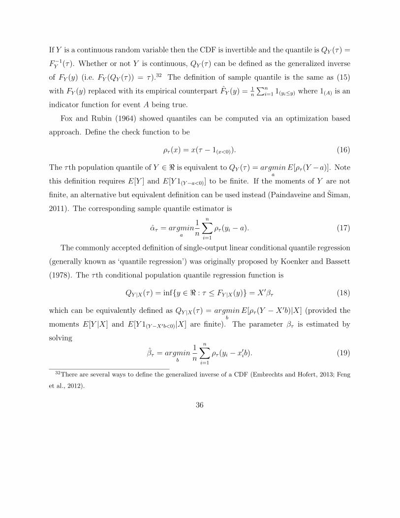
−1.0 −0.5 0.0 0.5 1.0

−1.

0−

0.5

0.0

0.5

1.0

Y1

Y2

β = 0

β = 0.2 β = 1 β = 10 β = 100

−1.0 −0.5 0.0 0.5 1.0

−1.

0−

0.5

0.0

0.5

1.0

Y1

Y2

β = 0

β = −0.2

β = −1

β = −10β = −100

−1.0 −0.5 0.0 0.5 1.0

−1.

0−

0.5

0.0

0.5

1.0

Y1

Y2

α = 0

α = 0.3 α = 0.6

α = −0.3

α = −0.6

−1.0 −0.5 0.0 0.5 1.0

−1.

0−

0.5

0.0

0.5

1.0

Y1

Y2

α = 0

α = 0.3 α = 0.6 α = 0α = 0.3

α = 0.6

β = 0β = 1

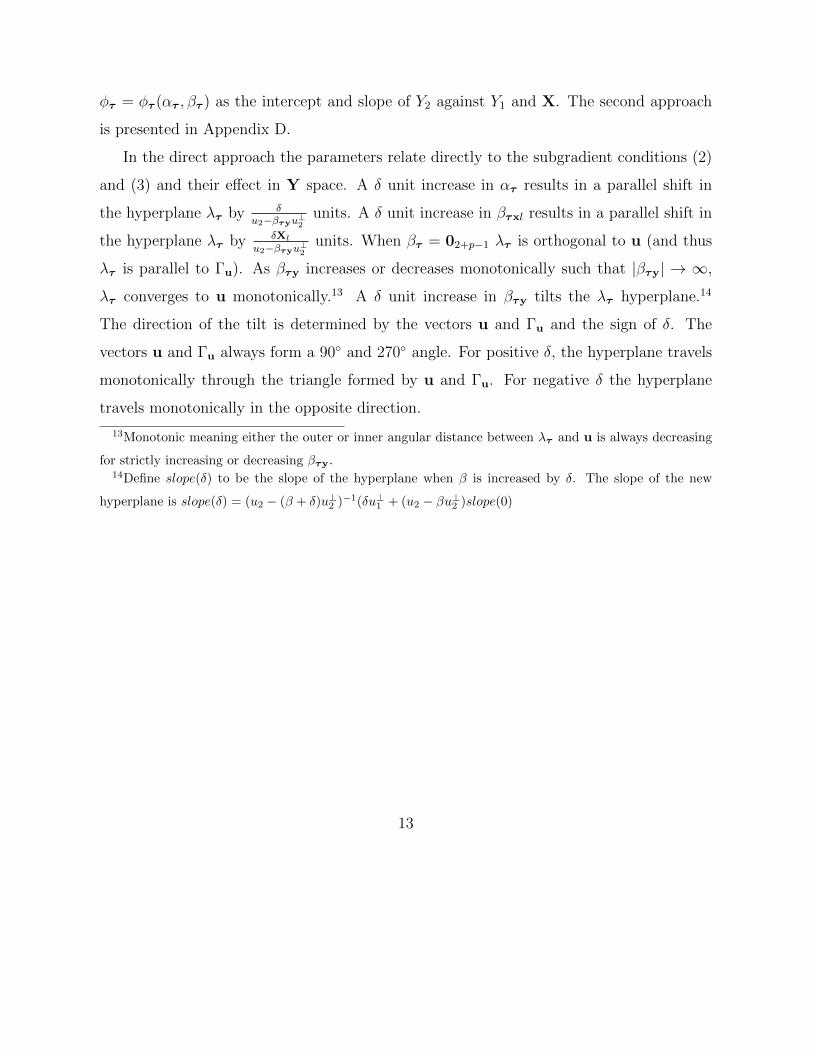
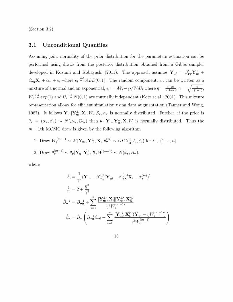
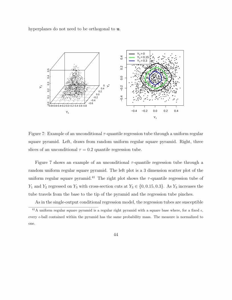
Figure 1: Implied λτ from various hyperparameters (τ subscript omitted). Top left, positive

increasing β. Top right, negative decreasing β. Bottom left, different αs. Bottom right,

different αs and βs.

Figure 1 shows prior λτ implied from the center of the prior with various hyperparam-

14

eters. For all four plots k = 2, the directional vector is u = ( 1√2, 1√

2) (black arrow) and

Γu = (− 1√2, 1√

2) (red arrow). The top left plot shows λτ for βτ increasing from 0 to 100 for

fixed ατ = 0. At βτ = 0 the hyperplane is perpendicular to u, as βτ increases λτ travels

counterclockwise until it becomes parallel to u. The top right plot shows the λτ for βτ

decreasing from 0 to −100 for fixed ατ = 0. At βτ = 0 λτ is perpendicular to u, as βτ

decreases λτ travels clockwise until it becomes parallel to u. The bottom left plot shows

λτ with ατ ranging from −0.6 to 0.6. The Tukey median can be thought of the point

(0, 0), then |ατ | is the distance of the intersection of u and λτ from the Tukey median.15

For positive ατ λτ is moving in the direction u and for negative ατ λτ is moving in the

direction −u. The bottom right plot shows λτ for various ατ and βτ . The solid black λτ

are for βτ = 0 and the dashed blue λτ are for βτ = 1 and ατ takes on values 0, 0.3 and 0.6

for both values of βτ . This plot confirms changes in ατ result in parallel shifts of λτ while

βτ tilts λτ .

If one is willing to accept joint normality of (ατ , βτ ) then a Gibbs sampler can be used.

The sampler is presented in Section 3.1. Further, if data is being collected and analyzed

in real time, then the prior of the current analysis can be centered over the estimates from

the previous analysis and the variance of the prior is the willingness the researcher is to

allow for departures from the previous analysis.

2.4 Conditional Quantiles

Quantile regression defined so far is unconditional on covariates. Thus the quantiles are

averaged over the covariate space. A conditional quantile provides local quantile estimates

conditional on covariates. A Bayesian multiple-output conditional quantile can be defined

15The Tukey median does not exist in these plots since there is no data. If there was data, the point

where u and Γu intersect would be the Tukey median.

15

from Hallin et al. (2015).16 A possible Bayesian approach is outlined but no proof of

consistency is provided. Consistency is checked via simulation in Section 4. The λτ hy-

perplanes are separately estimated for each conditioning value, thus the approach can be

computationally expensive. Define Mu = {(a,d) : a ∈ <, d ∈ <k subject to d′u = 1} the

population parameters are

(ατ ;x0 , δτ ;x0) = argmin(a,d)∈Mu

E[ρτ (d′Y − a)|X = x0].

If d = u − bΓ′u the population objective function can be rewritten as Ψc(a,b) =

E[ρτ (Yu − b′Y⊥u − a)|X = x0]. The population parameters are

(ατ ;x0 , βτ ;x0) = argmin(a,b)∈<k

Ψc(a,b). (5)

The subgradient conditions are

∂Ψc(a,b)

∂a

∣∣∣∣ατ ;x0 ,βτ ;x0

= Pr(Yu − β′τ ;x0Y⊥u − ατ ;x0 ≤ 0|X = x0)− τ = 0 (6)

and

∂Ψc(a,b)

∂b

∣∣∣∣ατ ;x0 ,βτ ;x0

= E[Y⊥u 1(Yu−β′τ ;x0Y⊥u−ατ ;x0≤0)|X = x0]− τE[Y⊥u |X = x0] = 0k−1. (7)

Assuming the distribution of X is continuous then the conditioning set has probability

0. Hallin et al. (2015) creates an empirical (frequentist) estimator using weights providing

larger weight to observations near x0. The estimator is

16This section omits theoretical discussion of multiple-output conditional quantiles. See Hallin et al.

(2015) for a rigorous exploration of the properties (including contours) for multiple-output conditional

quantiles.

16

θτ ;x0 = argminb

n∑i=1

Kh(Xi − x0)ρτ (Yui − bX rui) for r = c, l. (8)

The function Kh is a kernel function whose corresponding distribution has zero first

moment and positive definite second moment (e.g. uniform, Epanechnikov or Gaussian).

The parameter h determines bandwidth.17 If r = c then X cui = [1,Y⊥′ui ]

′ and the estimator

is called a local constant estimator. If r = l then X lui = [1,Y⊥′ui ]

′ ⊗ [1, (Xi − x0)′]′ and

the estimator is called a local bilinear estimator. The space that b is minimized over

is the real numbers of dimension equal to the length of X rui. For either value of r the

minimization can be expressed as maximization of an asymmetric Laplace likelihood with

a known (heteroskedastic) scale parameter.

The Bayesian approach assumes

Yu|X r, θτ ;x0 ∼ ALD(θ′τX r, Kh(X− x0)−1, τ)

whose density is

fτ (Y|X r, θτ ;x0 , Kh(X− x0)−1) = τ(1− τ)Kh(X− x0)exp(−Kh(X− x0)ρτ (Y − θ′τ ;x0X r))

∝ exp(−Kh(X− x0)ρτ (Y − θ′τ ;x0X r))

If the researcher assumes the prior distribution for θτ is normal then the parameters

can be estimated with a Gibbs sampler, which is presented in Section 3.2.

3 MCMC simulation

In this section a Gibbs sampler to obtain draws from the posterior distribution is presented

for unconditional regression quantiles (Section 3.1) and conditional regression quantiles

17To guarantee consistency of the frequentist estimator h must satisfy limn→∞

h = 0 and limn→∞

nhp−1n =∞.

Hallin et al. (2015) provides guidance for choosing h.

17

(Section 3.2).

3.1 Unconditional Quantiles

Assuming joint normality of the prior distribution for the parameters estimation can be

performed using draws from the posterior distribution obtained from a Gibbs sampler

developed in Kozumi and Kobayashi (2011). The approach assumes Yui = β′τyY⊥ui +

β′τxXi + ατ + εi where εiiid∼ ALD(0, 1). The random component, εi, can be written as a

mixture of a normal and an exponential, εi = ηWi+γ√WiUi where η = 1−2τ

τ(1−τ), γ =

√2

τ(1−τ),

Wiiid∼ exp(1) and Ui

iid∼ N(0, 1) are mutually independent (Kotz et al., 2001). This mixture

representation allows for efficient simulation using data augmentation (Tanner and Wong,

1987). It follows Yui|Y⊥ui,Xi,Wi, βτ , ατ is normally distributed. Further, if the prior is

θτ = (ατ , βτ ) ∼ N(µθτ ,Σθτ ) then θτ |Yu,Y⊥u ,X,W is normally distributed. Thus the

m+ 1th MCMC draw is given by the following algorithm

1. Draw W(m+1)i ∼ W |Yui,Y

⊥ui,Xi, θ

(m)τ ∼ GIG(1

2, δi, φi) for i ∈ {1, ..., n}

2. Draw θ(m+1)τ ∼ θτ |~Yu, ~Y

⊥u ,~X, ~W (m+1) ∼ N(θτ , Bτ ).

where

δi =1

γ2(Yui − β′(m)

τy Y⊥ui − β′(m)τx Xi − α(m)

τ )2

φi = 2 +η2

γ2

B−1τ = B−1

τ0 +n∑i=1

[Y⊥′ui ,X′i][Y

⊥′ui ,X

′i]′

γ2W(m+1)i

βτ = Bτ

(B−1τ0 βτ0 +

n∑i=1

[Y⊥′ui ,X′i]′(Yui − ηW (m+1)

i )

γ2W(m+1)i

)

18

and GIG(ν, a, b) is the Generalized Inverse Gamma distribution whose density is

f(x|ν, a, b) =(b/a)ν

2Kν(ab)xν−1exp(−1

2(a2x−1 + b2x)), x > 0,−∞ < ν <∞, a, b ≥ 0

and Kν(·) is the modified Bessel function of the third kind.18 To speed convergence the

MCMC sequence can be initialized with the frequentist estimate.19 The Gibbs sampler is

geometrically ergodic and thus the MCMC standard error is finite and the MCMC central

limit theorem applies (Khare and Hobert, 2012). This guarantees that after a long enough

burn-in draws from this sampler are equivalent to random draws from the posterior.

Numerous other algorithms can be used if the prior is non-normal. Kozumi and

Kobayashi (2011) provides a Gibbs sampler for when the prior is double exponential. Li

et al. (2010) and Alhamzawi et al. (2012) provide algorithms for when regularization is de-

sired. General purpose sampling schemes can also be used such as the Metropolis-Hastings,

slice sampling or other algorithms (Hastings, 1970; Neal, 2003; Liu, 2008).

The Metropolis-Hastings algorithm can be implemented as follows. Define the likelihood

to be Lτ (θτ ) =∏n

i=1 fτ (Yi|Xi, ατ , βτ , 1). Let the prior for θτ have the density πτ (θτ ).

Define g(θ†|θ) to be a proposal density. The m+1th MCMC draw is given by the following

algorithm

1. Draw θ†τ from g(θ†τ |θ(m)τ )

2. Compute A(θ†τ , θ(m)τ ) = min

(1, L(θ†τ )πτ (θ†τ )g(θ

(m)τ |θ†τ )

L(θ(m)τ )πτ (θ

(m)τ )g(θ†τ |θ

(m)τ )

)3. Draw u from Uniform(0, 1)

18An efficient sampler of the Generalized Inverse Gamma distribution was developed in Dagpunar (1989).

Implementations of the Gibbs sampler with a free σ parameter for R are provided in the package ‘bayesQR’

and ‘AdjBQR’ (Benoit and Van den Poel, 2017; Wang and Yang, 2016). However, the results presented in

this paper use a fixed σ = 1 parameter.19The R package ‘quantreg’ can provide such estimates (Koenker, 2018).

19

4. If u ≤ A(θ†τ , θ(m)τ ) set θ

(m+1)τ = θ†τ , else set θ

(m+1)τ = θ

(m)τ

Estimation of τ -quantile contours (see Appendix A) requires the simultaneous estima-

tion of several different λτ . Simultaneous estimation of multiple λτm (m ∈ {1, 2, ...,M}) can

be performed by creating an aggregate likelihood. The aggregate likelihood is the product of

the likelihoods for eachm, Lτ1,τ2,...,τM (ατ1 , βτ1 , ατ2 , βτ2 , ..., ατM , βτM ) =∏M

m=1 Lτm(ατm , βτm).

The prior is then defined for the vector (ατ1 , βτ1 , ατ2 , βτ2 , ..., ατM , βτM ). The Gibbs algo-

rithm can easily be modified for fixed τ to accommodate simultaneous estimation. To

estimate the parameters from various τ , the values of η and γ need to be adjusted appro-

priately.

3.2 Conditional Quantiles

Sampling from the conditional quantile posterior is similar to that of unconditional quan-

tiles except the likelihood is heteroskedastic with known heteroskedasticity. The approach

assumes Yui = θ′τX ri + Kh(X r

i − x0)−1εi where εiiid∼ ALD(0, 1). The random compo-

nent, Kh(X ri − x0)−1εi, can be written as a mixture of a normal and an exponential,

Kh(X ri −x0)−1εi = ηVi+γ

√Kh(X r

i − x0)−1ViUi where Vi = Kh(X ri −x0)−1Wi. If the prior

is θτ = (ατ , βτ ) ∼ N(µθτ ,Σθτ ) then a Gibbs sampler can be used. The m + 1th MCMC

draw is given by the following algorithm

1. Draw V(m+1)i ∼ W |Yui,X r

i , θ(m)τ ∼ GIG(1

2, δi, φi) for i ∈ {1, ..., n}

2. Draw θ(m+1)τ ∼ θτ |~Yu, ~Y

⊥u ,

~X r, ~W (m+1) ∼ N(θτ , Bτ ).

20

where

δi =Kh(X r

i − x0)

γ2(Yui − θ′(m)

τ X ri )2

φi = 2Kh(X ri − x0) +

η2Kh(X ri − x0)

γ2

B−1τ = B−1

τ0 +n∑i=1

Kh(X ri − x0)X r

i X r′i

γ2W(m+1)i

βτ = Bτ

(B−1τ0 βτ0 +

n∑i=1

Kh(X ri − x0)X r

i (Yui − ηW (m+1)i )

γ2W(m+1)i

).

The MCMC sequence can be initialized with the frequentist estimate.20 A Metropolis-

Hastings algorithm similar to the unconditional model can be used where L(θτ ) =∏n

i=1 fτ (Yi|X ri , θτ , Kh(X r

i −

x0)−1). Simultaneous estimation of many λτm is similar to the unconditional model.

4 Simulation

This section verifies pointwise consistency of the unconditional and conditional models.

Asymptotic coverage probability of the unconditional location model using the results from

Section 2.2 is also verified. Pointwise consistency is verified by checking convergence to so-

lutions of the subgradient conditions (population parameters). Four DGPs are considered.

1. Y ∼ Uniform Square

2. Y ∼ Uniform Triangle

3. Y ∼ N(µ,Σ), where µ = 02 and Σ =

1 1.5

1.5 9

20The R package ‘quantreg’ can provide such estimates using the weights option.

21

4. Y = Z +

0

X

where

XZ

∼ N

µXµZ

,ΣXX ΣXZ

Σ′XZ ΣZZ

,

ΣXX = 4, ΣXZ =

0

2

, ΣZZ =

1 1.5

1.5 9

, µX = 0 and µZ = 02

The first DGP has corners at (−12,−1

2), (−1

2, 1

2), (1

2,−1

2), (1

2, 1

2). The second DGP has

corners at (−12,− 1

2√

3), (1

2,− 1

2√

3), (0, 1√

3). DGPs 1,2 and 3 are location models and 4 is a

regression model. DGPs 1 and 2 conform to all the assumptions on the data generating pro-

cess. DGPs 3 and 4 are cases when Assumption 4 is violated. In DGP 4, the unconditional

distribution of Y is Y ∼ N

0

0

, 1 1.5

1.5 17

.

Two directions are considered, u = ( 1√2, 1√

2) and u = (0, 1). The orthogonal directions

are Γu = (1, 0) and Γu = (1/√

2,−1/√

2). The first vector is a 45o line between Y2 and Y1 in

the positive quadrant and the second vector points vertically in the Y2 direction. The depth

is τ = 0.2. The sample sample sizes are n ∈ {102, 103, 104}. The prior is θτ ∼ N(µθτ ,Σθτ )

where µθτ = 0k+p−1 and Σθτ = 1000Ik+p−1. The number of Monte Carlo simulations is 100

and for each Monte Carlo simulation 1,000 MCMC draws are used. The initial values are

set to the frequentist estimate.

4.1 Unconditional model pointwise consistency

Consistency for the unconditional model is verified by checking convergence to the solu-

tions of the subgradient conditions (population parameters). Convergence of subgradient

conditions (2) and (3) is verified in Appendix E.

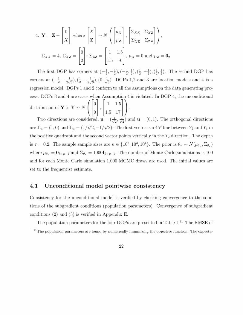
The population parameters for the four DGPs are presented in Table 1.21 The RMSE of

21The population parameters are found by numerically minimizing the objective function. The expecta-

22

the parameter estimates are presented in Tables 2, 3 and 4. The results show the Bayesian

estimator is converging to the population parameters.22

Data Generating Process

u θ 1 2 3 4

ατ -0.26 -0.20 -1.17 -1.16

(1/√

2, 1/√

2) βτy 0.00 0.44 -1.14 -1.17

βτx -0.18

ατ -0.30 -0.20 -2.19 -2.02

(0, 1) βτy 0.00 0.00 1.50 1.50

βτx 1.50

Table 1: Unconditional model population parameters

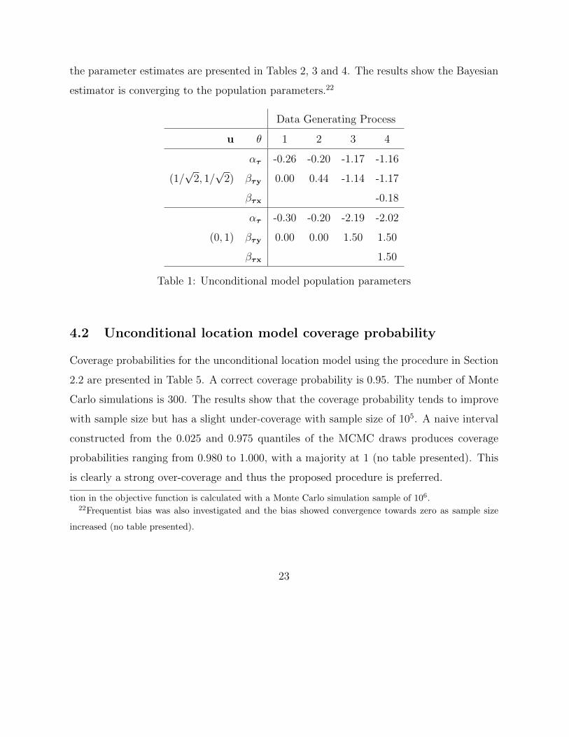
4.2 Unconditional location model coverage probability

Coverage probabilities for the unconditional location model using the procedure in Section

2.2 are presented in Table 5. A correct coverage probability is 0.95. The number of Monte

Carlo simulations is 300. The results show that the coverage probability tends to improve

with sample size but has a slight under-coverage with sample size of 105. A naive interval

constructed from the 0.025 and 0.975 quantiles of the MCMC draws produces coverage

probabilities ranging from 0.980 to 1.000, with a majority at 1 (no table presented). This

is clearly a strong over-coverage and thus the proposed procedure is preferred.

tion in the objective function is calculated with a Monte Carlo simulation sample of 106.22Frequentist bias was also investigated and the bias showed convergence towards zero as sample size

increased (no table presented).

23

Data Generating Process

θ n 1 2 3 4

102 5.70e-02 4.41e-02 2.20e-01 1.83e-01

ατ 103 1.49e-02 1.19e-02 6.80e-02 5.39e-02

104 4.30e-03 3.66e-03 1.97e-02 1.85e-02

102 9.63e-02 2.79e-01 9.61e-02 1.08e-01

βτy 103 3.63e-02 6.58e-02 3.15e-02 3.15e-02

104 1.19e-02 1.78e-02 1.07e-02 1.06e-02

Table 2: Unconditional model RMSE of parameter estimates (u = (1/√

2, 1/√

2))

4.3 Conditional model pointwise consistency

Convergence of the local constant conditional model is verified by checking convergence of

the Bayesian estimator to the parameters minimizing the population objective function (5).

The local constant specification is presented because that is the specification used in the ap-

plication. The conditional distribution of DGP 4 is Y |X = x0 ∼ N

0

x0/2

, 1 1.5

1.5 8

.

Thus the population objective function can be calculated using Monte Carlo integration

or with quadrature methods. The population parameters with x0 = 1 are (ατ ;1, βτ ;1) =

(−1.23, 1.167) for u = (1/√

2, 1/√

2) and (ατ ;1, βτ ;1) = (−1.53, 1.49) for u = (0, 1), which

are found by numerically minimizing the Monte Carlo estimated population objective func-

tion.23 The weight function is set to Kh(Xi − x0) = 1√2πh2

exp(− 1

2h2 (Xi − x0)2)

where

h =√

9σ2Xn−1/5.

Table 6 shows the RMSE of the Bayesian estimator for the conditional local constant

23The relative error difference between the Monte Carlo and quadrature methods was at most 5 · 10−3.

The Monte Carlo approach used a simulation sample of 106.

24

Data Generating Process

θ n 1 2 3 4

102 3.57e-02 2.23e-02 3.47e-01 2.94e-01

ατ 103 1.25e-02 5.59e-03 1.15e-01 1.13e-01

104 4.23e-03 2.10e-03 3.27e-02 3.36e-02

102 1.16e-01 7.03e-02 3.94e-01 2.78e-01

βτy 103 3.96e-02 1.61e-02 1.18e-01 1.17e-01

104 1.37e-02 6.73e-03 4.20e-02 3.13e-02

Table 3: Unconditional model RMSE of parameter estimates (u = (0, 1))

model. The estimator appears to be converging to the population parameter.

5 Application

The unconditional and conditional models are applied to educational data collected from

the Project STAR public access database. Project STAR was an experiment conducted on

11,600 students in 300 classrooms from 1985-1989 with interest of determining if reduced

classroom size improved academic performance.24 Students and teachers were randomly

selected in kindergarten to be in small (13-17 students) or large (22-26 students) class-

rooms.25 The students then stayed in their assigned classroom size throughout the fourth

grade. The outcome of the treatment was scores of mathematics and reading tests given

each year. This dataset has been analyzed many times before, see Finn and Achilles (1990);

24The data is publicly available at http://fmwww.bc.edu/ec-p/data/stockwatson.25This analysis omits large classrooms that had a teaching assistant.

25

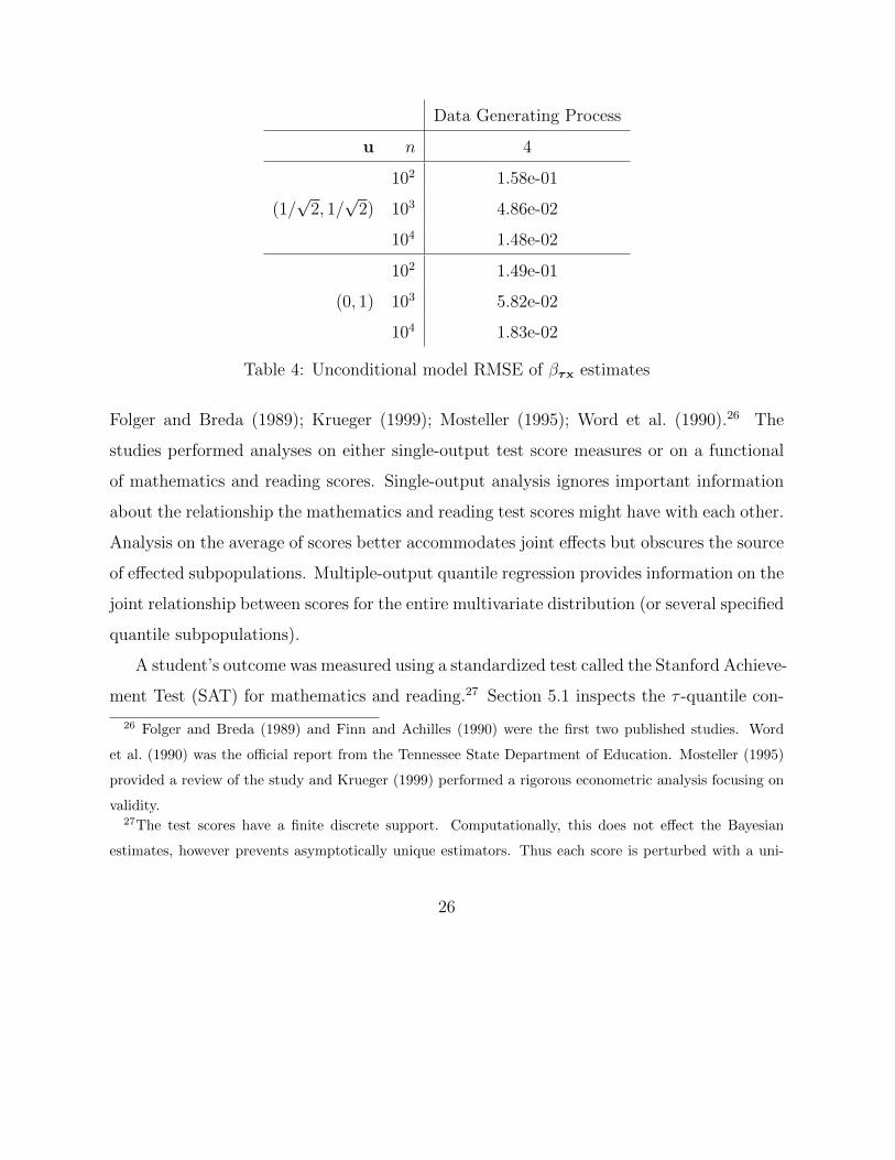
Data Generating Process

u n 4

102 1.58e-01

(1/√

2, 1/√

2) 103 4.86e-02

104 1.48e-02

102 1.49e-01

(0, 1) 103 5.82e-02

104 1.83e-02

Table 4: Unconditional model RMSE of βτx estimates

Folger and Breda (1989); Krueger (1999); Mosteller (1995); Word et al. (1990).26 The

studies performed analyses on either single-output test score measures or on a functional

of mathematics and reading scores. Single-output analysis ignores important information

about the relationship the mathematics and reading test scores might have with each other.

Analysis on the average of scores better accommodates joint effects but obscures the source

of effected subpopulations. Multiple-output quantile regression provides information on the

joint relationship between scores for the entire multivariate distribution (or several specified

quantile subpopulations).

A student’s outcome was measured using a standardized test called the Stanford Achieve-

ment Test (SAT) for mathematics and reading.27 Section 5.1 inspects the τ -quantile con-

26 Folger and Breda (1989) and Finn and Achilles (1990) were the first two published studies. Word

et al. (1990) was the official report from the Tennessee State Department of Education. Mosteller (1995)

provided a review of the study and Krueger (1999) performed a rigorous econometric analysis focusing on

validity.27The test scores have a finite discrete support. Computationally, this does not effect the Bayesian

estimates, however prevents asymptotically unique estimators. Thus each score is perturbed with a uni-

26

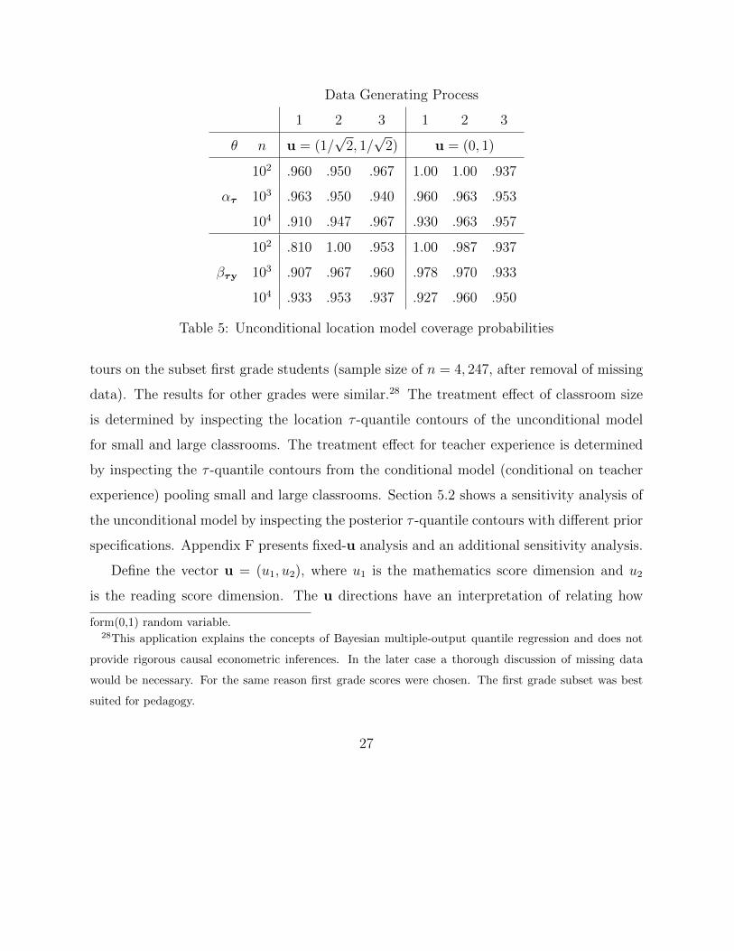
Data Generating Process

1 2 3 1 2 3

θ n u = (1/√

2, 1/√

2) u = (0, 1)

102 .960 .950 .967 1.00 1.00 .937

ατ 103 .963 .950 .940 .960 .963 .953

104 .910 .947 .967 .930 .963 .957

102 .810 1.00 .953 1.00 .987 .937

βτy 103 .907 .967 .960 .978 .970 .933

104 .933 .953 .937 .927 .960 .950

Table 5: Unconditional location model coverage probabilities

tours on the subset first grade students (sample size of n = 4, 247, after removal of missing

data). The results for other grades were similar.28 The treatment effect of classroom size

is determined by inspecting the location τ -quantile contours of the unconditional model

for small and large classrooms. The treatment effect for teacher experience is determined

by inspecting the τ -quantile contours from the conditional model (conditional on teacher

experience) pooling small and large classrooms. Section 5.2 shows a sensitivity analysis of

the unconditional model by inspecting the posterior τ -quantile contours with different prior

specifications. Appendix F presents fixed-u analysis and an additional sensitivity analysis.

Define the vector u = (u1, u2), where u1 is the mathematics score dimension and u2

is the reading score dimension. The u directions have an interpretation of relating how

form(0,1) random variable.28This application explains the concepts of Bayesian multiple-output quantile regression and does not

provide rigorous causal econometric inferences. In the later case a thorough discussion of missing data

would be necessary. For the same reason first grade scores were chosen. The first grade subset was best

suited for pedagogy.

27

u

θ n (1/√

2, 1/√

2) (0, 1)

102 2.90e-01 6.78e-01

ατ ,1 103 7.10e-02 3.04e-01

104 2.86e-02 1.33e-01

102 8.79e-02 3.22e-01

βτ ,1 103 3.35e-02 1.29e-01

104 1.53e-02 5.04e-02

Table 6: Local constant conditional model RMSE of parameter estimates

much relative importance the researcher wants to give to mathematics or reading. Define

u⊥ = (u⊥1 , u⊥2 ), where u⊥ is orthogonal to u. The components (u⊥1 , u

⊥2 ) have no meaningful

interpretation. Define mathematicsi to be the mathematics score of student i and readingi

to be the reading score of student i.

5.1 τ-quantile (regression) contours

The unconditional model is

Yui = mathematicsiu1 + readingiu2

Y⊥ui = mathematicsiu⊥1 + readingiu

⊥2

Yui = ατ + βτY⊥ui + εi

εiiid∼ ALD(0, 1, τ)

θτ = (ατ , βτ ) ∼ N(µθτ ,Σθτ ).

(9)

Unless otherwise noted, µθτ = 02 and Σθτ = 1000I2, meaning ex-ante knowledge is a weak

belief that the joint distribution of mathematics and reading has spherical Tukey depth

28

contours. The number of MCMC draws is 3,000 with a burn in of 1,000. The Gibbs

algorithm is initialized at the frequentist estimate.

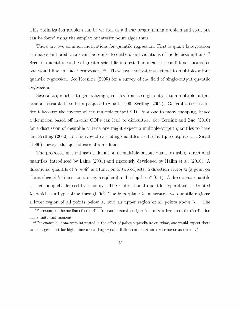
Figure 2 shows the τ -quantile contours for τ = 0.05, 0.20 and 0.40. A τ -quantile

contour is defined as the boundary of 23 in Appendix A. The data is stratified into smaller

classrooms (blue) and larger classrooms (black) and separate models are estimated for each.

The unconditional regression model was used but the effective results are conditional since

separate models are estimated by classroom size. The innermost contour is the τ = 0.40

region, the middle contour is the τ = 0.20 region and the outermost contour is the τ = 0.05

region. Contour regions for larger τ will always be contained in regions of smaller τ (if no

numerical error and priors are not contradictory). All the points that lie on the contour have

an estimated Bayesian Tukey depth of τ . The contours for larger τ capture the effects for

the more extreme students (e.g. students who perform exceptionally well on mathematics

and reading or exceptionally poorly on mathematics but well on reading). The contours for

smaller τ capture the effects for the more central or more ‘median’ student (e.g. students

who do not stand out from their peers). It can be seen that all the contours shift up and to

the right for the smaller classroom. This shows the centrality of mathematics and reading

scores improves for smaller classrooms compared to larger classrooms. This also all quantile

subpopulations of scores improve for students in smaller classrooms.29

29To claim all quantile subpopulations of scores improve would require estimating the τ -quantile regions

for all τ .

29

400 450 500 550 600 650 700

400

450

500

550

600

650

700

Mathematics Score

Rea

ding

Sco

re

Figure 2: τ -quantile contours. Blue represents small and black represents large classrooms.

Up to this point only quantile location models conditional on binary classroom size have

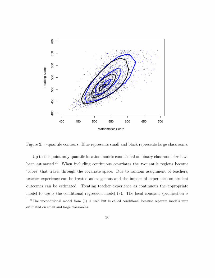
been estimated.30 When including continuous covariates the τ -quantile regions become

‘tubes’ that travel through the covariate space. Due to random assignment of teachers,

teacher experience can be treated as exogenous and the impact of experience on student

outcomes can be estimated. Treating teacher experience as continuous the appropriate

model to use is the conditional regression model (8). The local constant specification is

30The unconditional model from (1) is used but is called conditional because separate models were

estimated on small and large classrooms.

30

preferred if the researcher wishes to inspect slices of the regression tube. The local bilinear

specification is preferred if the researcher wishes to connect the slices of the regression tube

to create the regression tube. This analysis only looks at slices of the tube, thus the local

constant specification is used.

The conditional model is

Yui = mathematicsiu1 + readingiu2

Y⊥ui = mathematicsiu⊥1 + readingiu

⊥2

Xi = years of teacher experiencei

X lui = [1,Xi − x0,Y

⊥ui, (Xi − x0)Y⊥ui]

′

σ2X =

1

n− 1

n∑i=1

(Xi − X)2

h =√

9σ2Xn−1/5

Kh(Xi − x0) =1√

2πh2exp

(− 1

2h2(Xi − x0)2

)Yui = θτ ;x0Xui + εi

εiiid∼ ALD(0, Kh(Xi − x0)−1, τ)

θτ ;x0 ∼ N(µθτ ;x0,Σθτ ;x0

).

(10)

The prior hyperparameters are µθτ ;x0= 04 and Σθτ ;x0

= 1000I4. Small and large classrooms

are pooled together. Figure 3 shows the τ -quantile regression regions with a covariate for

experience. The values τ takes on are 0.20 (left plot) and 0.05 (right plot). The tubes are

sliced at x0 ∈ {1, 10, 20} years of teaching experience. The left plot shows reading scores

increase with teacher experience for the more ‘central’ students but there does not seem to

be a change in mathematics scores. The right plot shows a similar story for most of the

‘extreme’ students.

31

400 450 500 550 600 650 700

400

450

500

550

600

650

700

Mathematics Score

Rea

ding

Sco

reExp = 1Exp = 10Exp = 20

400 450 500 550 600 650 700

400

450

500

550

600

650

700

Mathematics ScoreR

eadi

ng S

core

Exp = 1Exp = 10Exp = 20

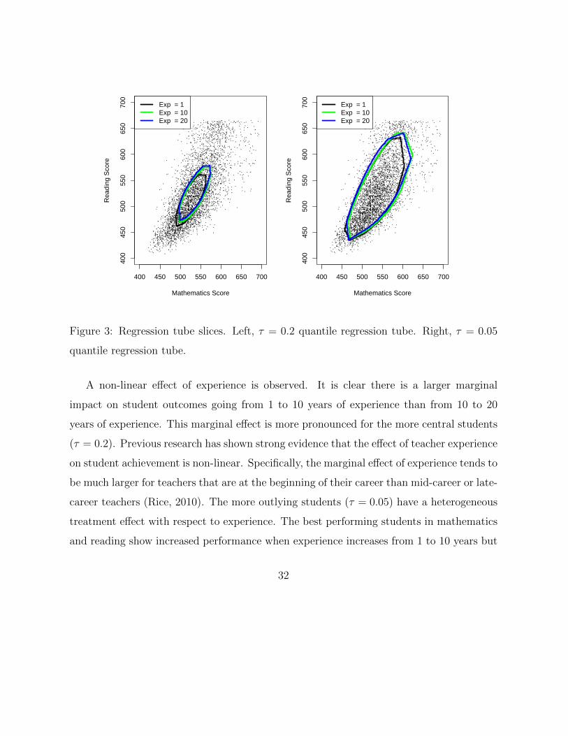
Figure 3: Regression tube slices. Left, τ = 0.2 quantile regression tube. Right, τ = 0.05

quantile regression tube.

A non-linear effect of experience is observed. It is clear there is a larger marginal

impact on student outcomes going from 1 to 10 years of experience than from 10 to 20

years of experience. This marginal effect is more pronounced for the more central students

(τ = 0.2). Previous research has shown strong evidence that the effect of teacher experience

on student achievement is non-linear. Specifically, the marginal effect of experience tends to

be much larger for teachers that are at the beginning of their career than mid-career or late-

career teachers (Rice, 2010). The more outlying students (τ = 0.05) have a heterogeneous

treatment effect with respect to experience. The best performing students in mathematics

and reading show increased performance when experience increases from 1 to 10 years but

32

little change after that. All other outlying students are largely unaffected by experience.

5.2 Sensitivity analysis

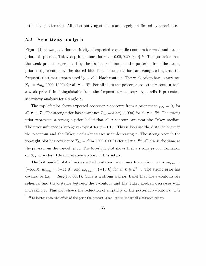
Figure (4) shows posterior sensitivity of expected τ -quantile contours for weak and strong

priors of spherical Tukey depth contours for τ ∈ {0.05, 0.20, 0.40}.31 The posterior from

the weak prior is represented by the dashed red line and the posterior from the strong

prior is represented by the dotted blue line. The posteriors are compared against the

frequentist estimate represented by a solid black contour. The weak priors have covariance

Σθτ = diag(1000, 1000) for all τ ∈ Bk. For all plots the posterior expected τ -contour with

a weak prior is indistinguishable from the frequentist τ -contour. Appendix F presents a

sensitivity analysis for a single λτ .

The top-left plot shows expected posterior τ -contours from a prior mean µθτ = 02 for

all τ ∈ Bk. The strong prior has covariance Σθτ = diag(1, 1000) for all τ ∈ Bk. The strong

prior represents a strong a priori belief that all τ -contours are near the Tukey median.

The prior influence is strongest ex-post for τ = 0.05. This is because the distance between

the τ -contour and the Tukey median increases with decreasing τ . The strong prior in the

top-right plot has covariance Σθτ = diag(1000, 0.0001) for all τ ∈ Bk, all else is the same as

the priors from the top-left plot. The top-right plot shows that a strong prior information

on βτy provides little information ex-post in this setup.

The bottom-left plot shows expected posterior τ -contours from prior means µθ0.05u =

(−65, 0), µθ0.20u = (−33, 0), and µθ0.40u = (−10, 0) for all u ∈ Sk−1. The strong prior has

covariance Σθτ = diag(1, 0.0001). This is a strong a priori belief that the τ -contours are

spherical and the distance between the τ -contour and the Tukey median decreases with

increasing τ . This plot shows the reduction of ellipticity of the posterior τ -contours. The

31To better show the effect of the prior the dataset is reduced to the small classroom subset.

33

effect is strongest for τ = 0.05.

400 450 500 550 600 650 700

400

450

500

550

600

650

700

Mathematics Score

Rea

ding

Sco

re

400 450 500 550 600 650 700

400

450

500

550

600

650

700

Mathematics Score

Rea

ding

Sco

re

400 450 500 550 600 650 700

400

450

500

550

600

650

700

Mathematics Score

Rea

ding

Sco

re

Figure 4: Tukey depth contour prior influence ex-post

6 Conclusion

A Bayesian framework for estimation of multiple-output directional quantiles was pre-

sented. The resulting posterior is consistent for the parameters of interest, despite having

a misspecified likelihood. By performing inferences as a Bayesian one inherits many of the

34

strengths of a Bayesian approach. The model is applied to the Tennessee Project STAR

experiment and it concludes that students in a smaller classroom perform better for every

quantile subpopulation than students in a larger classroom.

A possible avenue for future work is to find a structural economic model whose param-

eters relate directly to the subgradient conditions. This would give a contextual economic

interpretation of the subgradient conditions. Another possibility would be developing a for-

malized hypothesis test for the distribution comparison presented in Figure 2. This would

be a test for the ranking of multivariate distributions based off the directional quantile.

Appendix

A Review of single-output quantiles, Bayesian quan-

tiles and multiple-output quantiles

A.1 Quantiles and quantile regression

Quantiles sort and rank observations to describe how extreme an observation is. In one

dimension, for τ ∈ (0, 1), the τth quantile is the observation that splits the data into two

bins: a left bin that contains τ · 100% of the total observations that are smaller and a

right bin that contains the rest of the (1 − τ) · 100% total observations that are larger.

The entire family of τ ∈ (0, 1) quantiles allows one to uniquely define the distribution of

interest. Let Y ∈ < be a univariate random variable with Cumulative Density Function

(CDF) FY (y) = Pr(Y ≤ y) then the τth population single-output quantile is defined as

QY (τ) = inf{y ∈ < : τ ≤ FY (y)}. (15)

35

If Y is a continuous random variable then the CDF is invertible and the quantile is QY (τ) =

F−1Y (τ). Whether or not Y is continuous, QY (τ) can be defined as the generalized inverse

of FY (y) (i.e. FY (QY (τ)) = τ).32 The definition of sample quantile is the same as (15)

with FY (y) replaced with its empirical counterpart FY (y) = 1n

∑ni=1 1(yi≤y) where 1(A) is an

indicator function for event A being true.

Fox and Rubin (1964) showed quantiles can be computed via an optimization based

approach. Define the check function to be

ρτ (x) = x(τ − 1(x<0)). (16)

The τth population quantile of Y ∈ < is equivalent to QY (τ) = argmina

E[ρτ (Y −a)]. Note

this definition requires E[Y ] and E[Y 1(Y−a<0)] to be finite. If the moments of Y are not

finite, an alternative but equivalent definition can be used instead (Paindaveine and Siman,

2011). The corresponding sample quantile estimator is

ατ = argmina

1

n

n∑i=1

ρτ (yi − a). (17)

The commonly accepted definition of single-output linear conditional quantile regression

(generally known as ‘quantile regression’) was originally proposed by Koenker and Bassett

(1978). The τth conditional population quantile regression function is

QY |X(τ) = inf{y ∈ < : τ ≤ FY |X(y)} = X ′βτ (18)

which can be equivalently defined as QY |X(τ) = argminb

E[ρτ (Y − X ′b)|X] (provided the

moments E[Y |X] and E[Y 1(Y−X′b<0)|X] are finite). The parameter βτ is estimated by

solving

βτ = argminb

1

n

n∑i=1

ρτ (yi − x′ib). (19)

32There are several ways to define the generalized inverse of a CDF (Embrechts and Hofert, 2013; Feng

et al., 2012).

36

This optimization problem can be written as a linear programming problem and solutions

can be found using the simplex or interior point algorithms.

There are two common motivations for quantile regression. First is quantile regression

estimates and predictions can be robust to outliers and violations of model assumptions.33

Second, quantiles can be of greater scientific interest than means or conditional means (as

one would find in linear regression).34 These two motivations extend to multiple-output

quantile regression. See Koenker (2005) for a survey of the field of single-output quantile

regression.

Several approaches to generalizing quantiles from a single-output to a multiple-output

random variable have been proposed (Small, 1990; Serfling, 2002). Generalization is dif-

ficult because the inverse of the multiple-output CDF is a one-to-many mapping, hence

a definition based off inverse CDFs can lead to difficulties. See Serfling and Zuo (2010)

for a discussion of desirable criteria one might expect a multiple-output quantiles to have

and Serfling (2002) for a survey of extending quantiles to the multiple-output case. Small

(1990) surveys the special case of a median.

The proposed method uses a definition of multiple-output quantiles using ‘directional

quantiles’ introduced by Laine (2001) and rigorously developed by Hallin et al. (2010). A

directional quantile of Y ∈ <k is a function of two objects: a direction vector u (a point on

the surface of k dimension unit hypersphere) and a depth τ ∈ (0, 1). A directional quantile

is then uniquely defined by τ = uτ . The τ directional quantile hyperplane is denoted

λτ which is a hyperplane through <k. The hyperplane λτ generates two quantile regions:

a lower region of all points below λτ and an upper region of all points above λτ . The

33For example, the median of a distribution can be consistently estimated whether or not the distribution

has a finite first moment.34For example, if one were interested in the effect of police expenditure on crime, one would expect there

to be larger effect for high crime areas (large τ) and little to no effect on low crime areas (small τ).

37

lower region contains τ · 100% of observations and the upper region contains the remaining

(1− τ) · 100%. Additionally, the vector connecting the probability mass centers of the two

regions is parallel to u. Thus u orients the regression and can be thought of as a vertical

axis.

A.2 Bayesian single-output conditional quantile regression

Bayesian methods require a likelihood and hence an observational distributional assump-

tion. Yet quantile regression avoids making strong distributional assumptions (a seeming

contradiction). Yu and Moyeed (2001) introduced a Bayesian approach by using a pos-

sibly misspecified Asymmetric Laplace Distribution (ALD) likelihood.35 The Probability

Density Function (PDF) of the ALD(µ, σ, τ) is

fτ (y|µ, σ) =τ(1− τ)

σexp(− 1

σρτ (y − µ)). (20)

The Bayesian assumes Y |X ∼ ALD(X ′βτ , σ, τ), selects a prior and performs estimation

using standard procedures. The nuisance scale parameter can be fixed (typically at σ = 1)

or freely estimated.36 Sriram et al. (2013) showed posterior consistency for this model,

meaning that as sample size increases the probability mass of the posterior concentrates

around the values of β that satisfy (18). The result holds wether σ is fixed at 1 or freely

estimated. Yang et al. (2015) and Sriram (2015) provide a procedure for constructing

confidence intervals with correct frequentist coverage probability. If one is willing to accept

prior joint normality of βτ then a Gibbs sampler can be used to obtain random draws

from the posterior (Kozumi and Kobayashi, 2011). Alhamzawi et al. (2012) proposed using

35Note, the ALD maximum likelihood estimator is equal to the estimator from (19).36Rahman (2016) and Rahman and Karnawat (2019) are two examples where the scale parameter is used

in an ordinal model.

38

an adaptive Lasso sampler to provide regularization. Nonparametric Bayesian approaches

have been proposed by Kottas and Krnjajic (2009) and Taddy and Kottas (2010).

A.3 Unconditional multiple-output quantile regression

Any given λτ quantile hyperplane separates Y into two halfspaces. An open lower quantile

halfspace,

H−τ = H−τ (ατ , βτ ) = {y ∈ <k : u′y < β′τyΓ′uy + β′τxX + ατ}, (21)

and a closed upper quantile halfspace,

H+τ = H+

τ (ατ , βτ ) = {y ∈ <k : u′y ≥ β′τyΓ′uy + β′τxX + ατ}. (22)

Under certain conditions the distribution Y can be fully characterized by a family of

hyperplanes Λ = {λτ : τ = τu ∈ Bk} (Kong and Mizera, 2012, Theorem 5).37 There are

two subfamilies of hyperplanes: a fixed-u subfamily, Λu = {λτ : τ = τu, τ ∈ (0, 1)}, and a

fixed-τ subfamily, Λτ = {λτ : τ = τu,u ∈ Sk−1}. The τ subfamily is called a τ quantile

regression region (if no X is included then it is called a τ quantile region). The τ -quantile

(regression) region is defined as

R(τ) =⋂

u∈Sk−1

∩{H+τ }, (23)

where ∩{H+τ } is the intersection over H+

τ if (1) is not unique.

The boundary of R(τ) is called the τ -quantile (regression) contour. The boundary has a

strong connection to Tukey (i.e. halfspace) depth contours. Tukey depth is a multivariate

notion of centrality for some point y ∈ <k. Consider the set of all hyperplanes in <k that

37The conditions required are the directional quantile envelopes of the probability distribution of Y with

contiguous support have smooth boundaries for every τ ∈ (0, 0.5)

39

pass through y. The Tukey depth of y is the minimum of the percentage of observations

separated by each hyperplane passing through y. Hallin et al. (2010) showed the τ quantile

region is equivalent to the Tukey depth region.38 This provides a numerically efficient

approach to find Tukey depth contours.

If Y (and X for the regression case) is absolutely continuous with respect to Lebesgue

measure, has connected support and finite first moments then (ατ , βτ ) and λτ are unique

(Paindaveine and Siman, 2011).39 Under this assumption the ‘subgradient conditions’

required for consistency are well defined. It follows that Ψ(a,b) continuously differentiable

with respect to a and b and convex. The population parameters (ατ , βτ ) are defined as

the parameters that satisfy two subgradient conditions:

∂Ψ(a,b)

∂a

∣∣∣∣ατ ,βτ

= Pr(Yu − β′τyY⊥u − β′τxX− ατ ≤ 0)− τ = 0 (24)

and

∂Ψ(a,b)

∂b

∣∣∣∣ατ ,βτ

= E[[Y⊥u′,X′]′1(Yu−β′τyY⊥u−β′τxX−ατ≤)]− τE[[Y⊥u

′,X′]′] = 0k+p−1. (25)

The first condition can be written as Pr(Y ∈ H−τ ) = τ which retains the idea of a quantile

partitioning the support into two sets, one with probability τ and one with probability

(1− τ). The second condition is equivalent to

τ =E[Y⊥ui1(Y∈H−τ )]

E[Y⊥ui]for all i ∈ {1, ..., k − 1}

τ =E[Xi1(Y∈H−τ )]

E[Xi]for all i ∈ {1, ..., p}

38Mathematically, the Tukey (or halfspace) depth of y with respect to probability distribution P is

defined as HD(y, P ) = inf{P [H] : H is a closed halfspace containing y}. Then the Tukey halfspace depth

region is defined as D(τ) = {y ∈ <k : HD(y, P ) ≥ τ}. Hallin et al. (2010) show R(τ) = D(τ) for all

τ ∈ [0, 1).39This is Assumption 2, stated formally in Section 2.1.

40

Note that using the law of total expectations E[Y⊥ui1(Y∈H−τ )] = E[Y⊥ui|Y ∈ H−τ ]Pr(Y ∈

H−τ ) + 0Pr(Y /∈ H−τ ) = E[Y⊥ui|Y ∈ H−τ ]τ . Then the second condition can be rewritten as

E[Y⊥ui|Y ∈ H−τ ] = E[Y⊥ui] for all i ∈ {1, ..., k − 1}

E[Xi|Y ∈ H−τ ] = E[Xi] for all i ∈ {1, ..., p}.

Thus the probability mass center in the lower halfspace for the orthogonal response is

equal to the probability mass center in the entire orthogonal response space. Likewise for

the covariates, the probability mass center in the lower halfspace is equal to the probability

mass center in the entire covariate space.

The first k − 1 dimensions of the second subgradient conditions can also be rewritten

as Γ′uE[Y|Y ∈ H−τ ] = Γ′uE[Y] or equivalently Γ′u(E[Y|Y ∈ H−τ ]−E[Y]) = 0k−1, which is

satisfied if E[Y|Y ∈ H−τ ] = E[Y]. This sufficient condition interpretation states that the

probability mass center of the response in the lower halfspace is equal to the probability

mass center of the response in the entire space. However, this interpretation cannot be

guaranteed.

Further note, E[[Y⊥u′,X′]′] = E[[Y⊥u

′,X′]′1(Y∈H+

τ )] + E[[Y⊥u′,X′]′1(Y∈H−τ )]. Then the

second condition can be written as

diag(Γ′u, Ip)

[1

1− τE[[Y′,X′]′1(Y∈H+

τ )]−1

τE[[Y′,X′]′1(Y∈H−τ )]

]= 0k+p−1.

The first k − 1 components,

Γ′u

[1

1− τE[Y1(Y∈H+

τ )]−1

τE[Y1(Y∈H−τ )]

]= 0k−1,

show 11−τE[Y1(Y∈H+

τ )] − 1τE[Y1(Y∈H−τ )] is orthogonal to Γ′u and thus, is parallel to u. It

follows the difference of the weighted probability mass centers of the two spaces (H−τ and

H+τ ) is parallel to u.40

40Hallin et al. (2010) provides an additional interpretation in terms of Lagrange multipliers.

41

−0.4 −0.2 0.0 0.2 0.4

−0.

4−

0.2

0.0

0.2

0.4

Y1

Y2

●

●

Figure 5: Lower quantile halfspace for u = (1/√

2, 1/√

2) and τ = 0.2

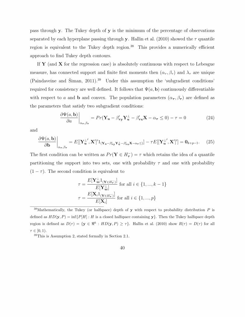
Subgradient conditions 2 and 3 can be visualized in Figure 5. The data, Y, are simu-

lated with 1, 000 independent draws from the uniform unit square centered on (0, 0). The

directional vector is u = (1/√

2, 1/√

2), represented by the orange 45◦ degree arrow. The

depth is τ = 0.2. The hyperplane λτ is the red dotted line. The lower quantile region,

H−τ , includes the red dots lying below λτ . The upper quantile region, H+τ , includes the

black dots lying above λτ . The probability mass centers of the lower and upper quantile

regions are the solid blue dots in their respective regions. The first subgradient condition

states that 20% of all points are red. The second subgradient condition states that the line

joining the two probability mass centers is parallel to u.

42

−0.4 −0.2 0.0 0.2 0.4

−0.

4−

0.2

0.0

0.2

0.4

Y1

Y2

−0.4 −0.2 0.0 0.2 0.4

−0.

4−

0.2

0.0

0.2

0.4

Y1

Y2

0.010.050.10.20.30.40.50.60.70.80.90.950.99

Figure 6: Example of a τ -quantile region and fixed-u halfspaces. Left, fixed τ = 0.2 quantile

region. Right, fixed u = (1/√

2, 1/√

2) quantile halfspaces.

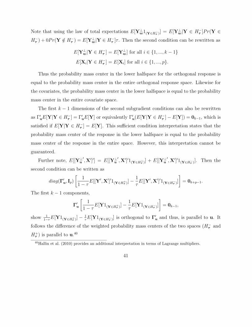
Figure 6 shows an example of a τ -quantile region (left) and fixed-u (right) halfspaces.

The left plot shows fixed-τ -quantile upper halfspace intersections of 32 equally spaced

directions on the unit circle for τ = 0.2. Any points on the boundary have Tukey depth

0.2. All points within the shaded blue region have a Tukey depth greater than or equal to

0.2 and all points outside the shaded blue region have Tukey depth less than 0.2.

The right plot of Figure 6 plot shows 13 quantile hyperplanes λτ for a fixed u =

(1/√

2, 1/√

2) with various τ (provided in the legend). The orange arrow shows the direction

vector u. The hyperplanes split the square such that τ · 100% of all points lie below the

hyperplanes. The weighted probably mass centers (not shown) are parallel to u. Note the

43

hyperplanes do not need to be orthogonal to u.

−0.8−0.6−0.4−0.2 0.0 0.2 0.4 0.6 0.8

0.0

0.1

0.2

0.3

0.4

0.5

−0.6−0.4

−0.2 0.0

0.2 0.4

0.6

Y1

Y2

Y3

●

●

●

●

●

●

●

●

●

●

●

●

●

●

●

●

●

●

●

●

●

●

●

●

●

●

●

●

●

●

●

●●

●

●

●

●

●

●

●

●

●

●

●

●

●

●

●

●

●

●

●

●

●

●

●

●

●

●

●

●●

●

●

●

●

●

●

●

●

●

●

●

●

●

●

●

●

●

●

●

●

●

●

●

●

●

●

●

●

●

●

●

●

●

●

●

●

●

●

●

●

●

●

●

●

●

●

●

●

●●

●

●

●

●

●

●

●

●

●

●

●

●

●

●

●

●

●

●

●

●

●

●

●

●

●

●

●

●

●

●

●

●

●

●

●

●

●

●

●

●

●

●

●

●

●

●

●

●

●

●

●

●

●

●●

●

●

●

●

●

●

●

●

●

●

●

●

●

●

●

●

●

●●

●

●

●

●

●

●

●

●

●

●

●

●

●

●

●

●

●

●

●

●

●

●

●

●

●

●

●

●

●

●

●

●

●

●

●

●

●

●

●

●

●

●

●

●

●

●

●●

●

●

●

●

●

●

●

●

●

●

●

●

●

●

●

●

●

●

●

●

●●

●

●

●

●

●

●

●

●

●

●

●

●

●

●

●

●

●

●

●

●

●

●

●

●

●

●

●

●

●

●

●

●

●

●

●

●

●

●

●

●

●

●

●

●

●

●

●

●

●

●

●

●

●

●

●

●

●

●

●

●

●

●

●

●

●

●

●

●

●

●

●

●

●

●

●

●

●

●

●●

●

●

●

●

●

●

●

●

●

●

●

●

●

●

●

●

●

●

●

●

●

●

●

●

●

●

●

●

●

●

●

●

●

●

●

●

●

●

●

●

●●

●

●

●

●

●

●

●

●

●●

●

●

●

●

●

●

●

●

●

●

●

●

●

●

●

●

●

●●

●

●

●

●

●

●

●

●

●

●

●

●

●

●

●

●

●

●

●

●

●

●

●

●●

●

●

●

●

●

●

●

●

●

●

●

●

●

●

●

●

●

● ●

●

●

●

●

●

●

●

●

●

●

●

●

●

●

●

●

●

●

●

●●

●

●

●

●

●

●

●

●

●

●

●

● ●

●

●

●

●

●

●

●

●

●

●

●

●

●

●

●

●

●

●

●

●

●

●●

●

●

●

●

●

●

●

●

●

●

●

●

●

●

●

●

●

●

●

●

●

●

●

●

●

●

●

●

●

●

●

●

●

●

●

●

●

● ●

●

●

●

●

●

●

●

●

●

●

●

●

●

●

●

●

●

●

●

●

●

●

●

●

●

●

●

●

●

●

●

●

●

●

●

●

●

●

●

●

●

●

●

●

●●

●

●●

●

●

●

●

●

●

●

●

●

●

●

●

●

●

●●

●

●

●

●

●

●

● ●

●

●

●

●

●

●

●

●

●

●

●

●

●

●

●

●

●

●

●

●

●

●

●

●

●

●

●

●

●

●

● ●

●

●

●

●

●

●

●

●

●

●

●

●

● ●

●

●

●

●

●

●

●

●

●

●

●

●

●

●

●

●

●

●●

●

●

●

●

●

●

●

●

●

●

●

●

●

●

●

●

●

●

●

●●

●

●

●

●

●

●

●

●

●

●

●

●

●

●

●

●

●

●

●

●

●

●

●

●

●

●

●

●

●

●

●

●

●

●

●

●

●

●

●

●●

●

●

●

●

●

●

●

●

●

●

●

●

●

●

●

●

●

●

●

●●

●

●

●

●

●

●

●

●

●

●

●

●

●

●

●

●

●

●

●

●

●

●

● ●

●

●

●

●

●

●

●

●

●

●

●

●

●

●

●

●

●

●

●

●

●

●

●

●

●

●

●

●

●

●

●

●

●

●

●

●

●

●

●

●

●

●

●

●

●

●

●

●

●

●

●

●

●

●

●

●

●

●

●●

●

●

●

●

●

●

●

●

●

●

●

●●

●

●

●

●

●

●

●

●

●

●

●

●

●

●

●

●

●

●

●

●

●

●

●

●

●

●

●

●

●

●

●

●

●

●

●

●

●

●

●

●●

●

●

●

●

●

●

●

●

●

●

●

●

●

●

●

●

●

●

●

●

●

●

●

●

●

●

●

●

●

●

●

●

●

●

●

●

●

●

●

●

●

●

●

●●

●

●

●

●

●

●

●

●

●

●

●

●

●

●

●

●

●

●

●

●

●

●

●

●

●

●

●

●

●

●

●

●

●

●

●

●

●

●

●

●

●

●

●

●

●

●

●

●

●

−0.4 −0.2 0.0 0.2 0.4

−0.

4−

0.2

0.0

0.2

0.4

Y1

Y2

Y3 = 0Y3 = 0.15Y3 = 0.3

Figure 7: Example of an unconditional τ -quantile regression tube through a uniform regular

square pyramid. Left, draws from random uniform regular square pyramid. Right, three

slices of an unconditional τ = 0.2 quantile regression tube.

Figure 7 shows an example of an unconditional τ -quantile regression tube through a

random uniform regular square pyramid. The left plot is a 3 dimension scatter plot of the

uniform regular square pyramid.41 The right plot shows the τ -quantile regression tube of

Y1 and Y2 regressed on Y3 with cross-section cuts at Y3 ∈ {0, 0.15, 0.3}. As Y3 increases the

tube travels from the base to the tip of the pyramid and the regression tube pinches.

As in the single-output conditional regression model, the regression tubes are susceptible

41A uniform regular square pyramid is a regular right pyramid with a square base where, for a fixed ε,

every ε-ball contained within the pyramid has the same probability mass. The measure is normalized to

one.

44

to quantile crossing. Meaning if one were to trace out the entire regression tube along Y3

for a given τ and τ † > τ , the regression tube for τ † might not be contained in the one for

τ for all Y3.

B Proof of Theorem 1

In this section consistency of the posterior for the population parameters is proven. This

proof is for the location case. The regression case should come with easy modification by

concatenating βτy with βτx and Y⊥ui with Xi. Since Y and X rely on the same sets of

assumptions, and expectations and probabilities are taken over Y and X, there should not

be any issue with these results generalizing to the regression case. For ease of readability

τ is omitted from ατ , βτ and Πτ .

Define the population parameters (α0, β0) to be the parameters that satisfy (2) and (3).

Note that the posterior can be written equivalently as

Π(U |(Y1,X1), (Y2,X2), ..., (Yn,Xn)) =

∫U

∏ni=1

fτ (Yi|Xi,α,β,σ)fτ (Yi|Xi,α0,β0,σ0)

dΠ(α, β)∫Θ

∏ni=1

fτ (Yi|Xiα,β,σ)fτ (Yi|Xi,α0,β0,σ0)

dΠ(α, β)(26)

Writing the posterior in this form is for mathematical convenience. Define the posterior

numerator to be

In(U) =

∫U

n∏i=1

fτ (Yi|α, β, σ)

fτ (Yi|α0, β0, σ)dΠ(α, β). (27)

The posterior denominator is then In(Θ). The next lemma (presented without proof)

provides several inequalities that are useful later.

Lemma 1. Let bi = (α−α0) + (β− β0)′Y⊥ui, Wi = (u′− β′0Γ′u)Yi−α0, W+i = max(Wi, 0)

and W−i = min(−Wi, 0). Then a) log

(fτ (Yi|α,β,σ)fτ (Yi|α0,β0,σ)

)=

45

1

σ

−bi(1− τ) if (u′ − β′Γ′u)Yi − α ≤ 0 and (u′ − β′0Γ′u)Yi − α0 ≤ 0

−((u′ − β′0Γ′u′)Yi − α0) + biτ if (u′ − β′Γ′u)Yi − α > 0 and (u′ − β′0Γ′u)Yi − α0 ≤ 0

(u′ − β′Γ′u)Yi − α + biτ if (u′ − β′Γ′u)Yi − α ≤ 0 and (u′ − β′0Γ′u)Yi − α0 > 0

biτ if (u′ − β′Γ′u)Yi − α > 0 and (u′ − β′0Γ′u)Yi − α0 > 0

b) log(

fτ (Yi|α,β,σ)fτ (Yi|α0,β0,σ)

)≤ 1

σ|bi| ≤ |α− α0|+ |(β − β0)′||Γ′u||Yi|

c) log(

fτ (Yi|α,β,σ)fτ (Yi|α0,β0,σ)

)≤ 1

σ|(u′ − β′0Γ′u)Yi − α0| ≤ 1

σ(|(u′ − β′0Γ′u)||Yi|+ |α0|)

d) log(

fτ (Yi|α,β,σ)fτ (Yi|α0,β0,σ)

)= 1

σ

−bi(1− τ) + min(W+i , bi) if bi > 0

biτ + min(W−i ,−bi) if bi ≤ 0

e) log(

fτ (Yi|α,β,σ)fτ (Yi|α0,β0,σ)

)≥ − 1

σ|bi| ≥ −|α− α0| − |(β − β0)′||Γ′u||Yi|

The next lemma provides more useful inequalities.

Lemma 2. The following inequalities hold:

a) E[log(

fτ (Yi|α,β,σ)fτ (Yi|α0,β0,σ)

)]≤ 0

b) σE[log(

fτ (Yi|α,β,σ)fτ (Yi|α0,β0,σ)

)]= E

[−(Wi − bi)1(bi<Wi<0)

]+ E

[(Wi − bi)1(0<Wi<bi)

]c) σE

[log(

fτ (Yi|α,β,σ)fτ (Yi|α0,β0,σ)

)]≤ E [−(Wi − bi)]Pr(bi < Wi < 0) + E [(Wi − bi)]Pr(0 <

Wi < bi)

d) σE[log(

fτ (Yi|α,β,σ)fτ (Yi|α0,β0,σ)

)]≤ −E

[− bi

21(bi<0)

]Pr( bi

2< Wi < 0) − E

[bi2

1(0<bi)

]Pr(0 <

Wi <bi2

)

e) if Assumption 4 holds then limn→∞

1n

∑ni=1 E[|Wi|] <∞.

Proof. Note that E[bi] = (α−α0)+(β−β0)′E[Y⊥ui] = (α−α0)+ 1τ(β−β0)′E[Y⊥ui1((u′−β′0Γ′u)Yi−α0≤0)]

from subgradient condition (12). Define Ai to be the event (u′− β′0Γ′u)Yi−α0 ≤ 0 and Aci

46

it’s complement. Define Bi to be the event (u′−β′Γ′u)Yi−α ≤ 0 and Bci it’s complement.

σ log

(fτ (Yi|α, β, σ)

fτ (Yi|α0, β0, σ)

)= biτ − bi1(Ai,Bi) − ((u′ − β′0Γ′u)Yi − α0)1(Ai,Bci ) + ((u′ − β′Γ′u)Yi − α)1(Aci ,Bi)

= biτ − bi1(Ai) + (bi − ((u′ − β′0Γ′u)Yi − α0))1(Ai,Bci ) + ((u′ − β′Γ′u)Yi − α)1(Aci ,Bi)

= biτ − bi1(Ai) − ((u′i − β′Γ′u)Yi − α)1(Ai,Bci ) + ((u′ − β′Γ′u)Yi − α)1(Aci ,Bi)

Since E[(α− α0)1(Ai)] = τ(α− α0) then E[biτ − bi1(Ai)] = 0. Then

σE

[log

(fτ (Yi|α, β, σ)

fτ (Yi|α0, β0, σ)

)]= E[−((u′−β′Γ′u)Yi−α)1(Ai,Bci )]+E[(u′−β′Γ′u)Yi−α)1(Aci ,Bi)

]

The constraint in the first term and second terms imply −((u′ − β′Γ′u)Yi − α) < 0 and

(u′ − β′Γ′u)Yi − α ≤ 0 over their respective support regions. It follows

σE

[log

(fτ (Yi|α, β, σ)

fτ (Yi|α0, β0, σ)

)]= E

[−(Wi − bi)1(bi<Wi<0)

]+ E

[(Wi − bi)1(0<Wi<bi)

].

Note that (Wi − bi)1(0<Wi<bi) ≤ (Wi − bi)1(0<Wi<bi2

)< − bi

21

(0<Wi<bi2

). Likewise, −(Wi −

bi)1(bi<Wi<0) <bi2

1(bi2<Wi<0)

. Thus,

σE

[log

(fτ (Yi|α, β, σ)

fτ (Yi|α0, β0, σ)

)]≤ E

[bi2

1(bi2<Wi<0)

]+ E

[−bi

21

(bi2>Wi>0)

].

Holders inequality with p = 1 and q =∞ implies σE[log(

fτ (Yi|α,β,σ)fτ (Yi|α0,β0,σ)

)]≤ −E

[− bi

21(bi<0)

]Pr( bi

2<

Wi < 0)− E[bi2

1(0<bi)

]Pr(0 < Wi <

bi2

).

The next proposition shows that the KL minimizer is the parameter vector that satisfies

the subgradient conditions.

47

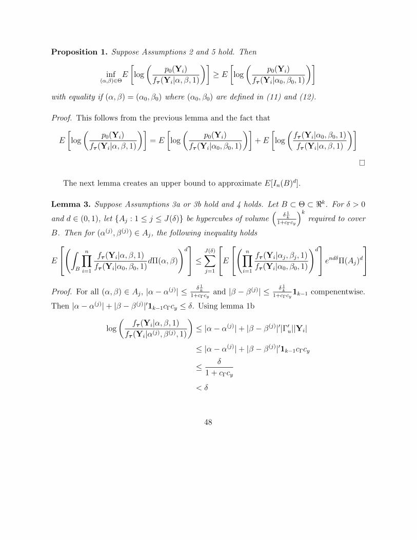
Proposition 1. Suppose Assumptions 2 and 5 hold. Then

inf(α,β)∈Θ

E

[log

(p0(Yi)

fτ (Yi|α, β, 1)

)]≥ E

[log

(p0(Yi)

fτ (Yi|α0, β0, 1)

)]with equality if (α, β) = (α0, β0) where (α0, β0) are defined in (11) and (12).

Proof. This follows from the previous lemma and the fact that

E

[log

(p0(Yi)

fτ (Yi|α, β, 1)

)]= E

[log

(p0(Yi)

fτ (Yi|α0, β0, 1)

)]+ E

[log

(fτ (Yi|α0, β0, 1)

fτ (Yi|α, β, 1)

)]

The next lemma creates an upper bound to approximate E[In(B)d].

Lemma 3. Suppose Assumptions 3a or 3b hold and 4 holds. Let B ⊂ Θ ⊂ <k. For δ > 0

and d ∈ (0, 1), let {Aj : 1 ≤ j ≤ J(δ)} be hypercubes of volume(

δ 1k

1+cΓcy

)krequired to cover

B. Then for (α(j), β(j)) ∈ Aj, the following inequality holds

E

(∫B

n∏i=1

fτ (Yi|α, β, 1)

fτ (Yi|α0, β0, 1)dΠ(α, β)

)d ≤ J(δ)∑

j=1

E( n∏

i=1

fτ (Yi|αj, βj, 1)

fτ (Yi|α0, β0, 1)

)d endδΠ(Aj)

d

Proof. For all (α, β) ∈ Aj, |α − α(j)| ≤ δ 1

k

1+cΓcyand |β − β(j)| ≤ δ 1

k

1+cΓcy1k−1 compenentwise.

Then |α− α(j)|+ |β − β(j)|′1k−1cΓcy ≤ δ. Using lemma 1b

log

(fτ (Yi|α, β, 1)

fτ (Yi|α(j), β(j), 1)

)≤ |α− α(j)|+ |β − β(j)|′|Γ′u||Yi|

≤ |α− α(j)|+ |β − β(j)|′1k−1cΓcy

≤ δ

1 + cΓcy

< δ

48

Then∫Aj

∏ni=1

fτ (Yi|α,β,1)fτ (Yi|α0,β0,1)

dΠ(α, β) =

n∏i=1

fτ (Yi|α(j), β(j), 1)

fτ (Yi|α0, β0, 1)

∫Aj

n∏i=1

fτ (Yi|α, β, 1)

fτ (Yi|α(j), β(j), 1)dΠ(α, β)

≤n∏i=1

fτ (Yi|α(j), β(j), 1)

fτ (Yi|α0, β0, 1)enδΠ(Aj)

Then E

[(∫B

∏ni=1

fτ (Yi|α,β,1)fτ (Yi|α0,β0,1)

dΠ(α, β))d]≤

E

J(δ)∑

j=1

(n∏i=1

fτ (Yi|α(j), β(j), 1)

fτ (Yi|α0, β0, 1)dΠ(α, β)

)enδΠ(Aj)

d

≤J(δ)∑j=1

E

( n∏i=1

fτ (Yi|α(j), β(j), 1)

fτ (Yi|α0, β0, 1)dΠ(α, β)

)d

endδ(Π(Aj))d

.The last inequality holds because (

∑i xi)

d ≤∑

i xdi for d ∈ (0, 1) and xi > 0.

Let U cn ⊂ Θ such that (α0, β0) 6∈ U c

n. The next lemma creates an upper bound for

the expected value of the likelihood within U cn. Break U c

n into a sequence of halfspaces,

{Vln}L(k)l=1 , such that

L(k)⋃l=1

Vln = U cn, where

V1n = {(α, β) : α− α0 ≥ ∆n, β1 − β01 ≥ 0, ..., βk − β0k ≥ 0}

V2n = {(α, β) : α− α0 ≥ 0, β1 − β01 ≥ ∆n, ..., βk − β0k ≥ 0}...

VL(k)n = {(α, β) : α− α0 < 0, β1 − β01 < 0, ..., βk − β0k ≤ −∆n}

for some ∆n > 0. This sequence makes explicit that the distance of at least one component

of the vector (α, β) is larger than it’s corresponding component of (α0, β0) by at least |∆n|.

49

How the sequence is indexed exactly is not important. The rest of the proof will focus on

V1n, the arguments for the other sets are similar. Define Bin = −E[log(

fτ (Yi|α,β,1)fτ (Yi|α0,β0,1)

)].42

Lemma 4. Let G ∈ Θ be compact. Suppose Assumption 4 holds and (α, β) ∈ G ∩ V1n.

Then there exists a d ∈ (0, 1) such that

E

[n∏i=1

(fτ (Yi|α, β, 1)

fτ (Yi|α0, β0, 1)

)d]≤ e−d

∑ni=1 Bin

Proof. Define hd(α, β) =1−E

[(fτ (Yi|α,β,1)

fτ (Yi|α0,β0,1)

)d]d

− E[log(

fτ (Yi|α,β,1)fτ (Yi|α0,β0,1)

)]. From the proof of

Lemma 6.3 in Kleijn and van der Vaart (2006), limd→0

hd(α, β) = 0 and hd(α, β) is a decreasing

function of d for all (α, β). Note that hd(α, β) is continuous in (α, β). Then by Dini’s

theorem hd(α, β) converges to hd(0,0k−1) uniformly in (α, β) as d converges to zero. Define

δ = inf(α,β)∈G

log(

fτ (Yi|α,β,1)fτ (Yi|α0,β0,1)

)then there exists a d0 such that 0 − hd0(α, β) ≤ δ

2. From

lemma 2a E[log(

fτ (Yi|α,β,1)fτ (Yi|α0,β0,1)

)]< 0. Then

E

[(fτ (Yi|α, β, 1)

fτ (Yi|α0, β0, 1)

)d0]≤ 1 + d0E

[log

(fτ (Yi|α, β, 1)

fτ (Yi|α0, β0, 1)

)]+ d0

δ

2

≤ 1 +d0

2E

[log

(fτ (Yi|α, β, 1)

fτ (Yi|α0, β0, 1)

)]≤ e

d02E[log(

fτYi|α,β,1)

fτ (Yi|α0,β0,1)

)]

The last inequality holds because 1 + t ≤ et for any t ∈ <.

The next lemma is used to show the numerator of the posterior, In(U cn), converges to

zero for sets U cn not containing (α0, β0).

42I would like the thank Karthik Sriram for help with the proof of the next lemma.

50

Lemma 5. Suppose Assumptions 3a, 4 and 6 hold. Then there exists a uj > 0 such that

for any compact Gj ⊂ Θ,∫Gcj∩Vjn

e∑ni=1 log

(fτ (Yi|α,β,1)

fτ (Yi|α0,β0,1)

)dΠ(α, β) ≤ e−nuj

for sufficiently large n.

Proof. Let

C0 =4 limn→∞

1m

∑mi=1E[|Wi|]

(1− τ)cp,

ε = min(εZ) and A = kBε = 2C0, where cp and εz are from Assumption 6. This limit exists

by Lemma 2e. Define

G1 = {(α, β) : (α− α0, β1 − β01, ..., βk − β0k) ∈ [0, A]× [0, B]× ...× [0, B]}.

If (α, β) ∈ Gc1 ∩ W1 then (α − α0) > A or (β − β0)j > B for some j. If Y⊥ui > ε then

bi = (α− α0) + (β − β0)′Y⊥ui > 2C0. Split the likelihood ratio as

n∑i=1

log

(fτ (Yi|α, β, 1)

fτ (Yi|α0, β0, 1)

)=

n∑i=1

log

(fτ (Yi|α, β, 1)

fτ (Yi|α0, β0, 1)

)1(Y⊥uij>εZj ,∀j) +

n∑i=1

log

(fτ (Yi|α, β, 1)

fτ (Yi|α0, β0, 1)

)(1− 1(Y⊥uij>εZj ,∀j)).

Since min(W+i , bi) ≤ W+

i ≤ |Wi| and using lemma 1 d,

n∑i=1

log

(fτ (Yi|α, β, 1)

fτ (Yi|α0, β0, 1)

)1(Y⊥uij > εZj,∀j) =

n∑i=1

(−bi(1− τ) +min(W+i , bi))1(Y⊥uij>εZj ,∀j)

≤n∑i=1

(−2C0(1− τ) + |Wi|)1(Y⊥uij>εZj ,∀j).

From lemma 1b and for large enough n then

n∑i=1

log

(fτ (Yi|α, β, 1)

fτ (Yi|α0, β0, 1)

)1(Y⊥uij>εZj ,∀j) ≤

n∑i=1

|Wi|(1− 1(Y⊥uij>εZj ,∀j)).

51

Then for large enough n

n∑i=1

log

(fτ (Yi|α, β, 1)

fτ (Yi|α0, β0, 1)

)≤ −nC0(1− τ)Pr(Y⊥uij > εZj, ∀j) + 2n lim

n→∞

1

m

m∑i=1

E[|Wi|]

= −2n limn→∞

1

m

m∑i=1

E[|Wi|]

= −1

2nC0(1− τ)Pr(Y⊥uij > εZj,∀j)

Thus the result holds when ui = 12C0(1− τ)Pr(Y⊥uij > εZj,∀j).

The next lemma shows the marginal likelihood, In(Θ), goes to infinity at the same rate

as the numerator in the previous lemma.

Lemma 6. Suppose Assumptions 3a and 4 holds, then∫Θ

e∑ni=1 log

(fτ (Yi|α,β,1)

fτ (Yi|α0,β0,1)

)dΠ(α, β) ≥ e−nε.

Proof. From Lemma 1e log(

fτ (Yi|α,β,1)fτ (Yi|α0,β0,1)

)≥ −|bi| ≥ −|α− α0| − |β − β0|′|Γu||Yi|. Define

Dε =

{(α, β) : |α− α0| <

1kε

1 + cΓcy, |β − β0| <

1kε

1 + cΓcy1k−1 componentwise

}.

Then for (α, β) ∈ Vε

log

(fτ (Yi|α, β, 1)

fτ (Yi|α0, β0, 1)

)≥ −|α− α0| − |β − β0|′|Γu||Yi|

≥ −|α− α0| − |β − β0|′1k−1cΓcy

≥ − ε

1 + cΓcy

> −ε

Then∑n

i=1 log(

fτ (Yi|α,β,1)fτ (Yi|α0,β0,1)

)≥ −nε. If Π(·) is proper, then Π(Dε) ≤ 1.

52

The previous two lemmas imply the posterior is converging to zero in a restricted

parameter space.

Lemma 7. Suppose Assumptions 4, and 6 hold. Then for each l ∈ {1, 2, ..., L(k)}, there

exists a compact Gl such that

limn→∞

Π(Vln ∩Gcl |Y1, ...,Yn) = 0.

Proof. Let ε from Lemma 6 equal ui4

from Lemma 5. Then∫Θ

e∑ni=1 log

(fτ (Yi|α,β,1)

fτ (Yi|α0,β0,1)

)dΠ(α, β) ≥

∫Dε

e∑ni=1 log

(fτ (Yi|α,β,1)

fτ (Yi|α0,β0,1)

)dΠ(α, β)

≥ e−nεdΠ(Dε)

Then limn→∞

∫Θe∑ni=1 log

(fτ (Yi|α,β,1)

fτ (Yi|α0,β0,1)

)dΠ(α, β)enuj/2 =∞ and

limn→∞

∫Vjn∩Gcj

e∑ni=1 log

(fτ (Yi|α,β,1)

fτ (Yi|α0,β0,1)

)dΠ(α, β)enuj/2 = 0.

The next proposition bounds the expected value of the numerator, E[In(V1n∩G)d], and

the denominator, In(Θ), of the posterior. Define Bin = −E[log(

fτ (Yi|α,β,1)fτ (Yi|α0,β0,1)

)].

Lemma 8. Suppose Assumptions 3a and 4 hold. Define

Dδn ={

(α, β) : |α− α0| <1kδn

1+cΓcy, |β − β0| <

1kδn

1+cΓcy1k−1 componentwise

}. Then for (α, β) ∈

Dδn

1. There exists a δn ∈ (0, 1) and fixed R > 0 such that

E

(∫V1n∩G

n∏i=1

fτ (Yi|α, β, 1)

fτ (Yi|α0, β0, 1)dΠ(α, β)

)d ≤ ed

∑ni=1BinendδnR2/δ2

n

2. ∫Θ

n∏i=1

fτ (Yi|α, β, 1)

fτ (Yi|α0, β0, 1)dΠ(α, β) ≥ e−nδnΠ(Dδn)

53

Proof. From Lemma 3 and 4 E

[(∫W1n∩G

∏ni=1

fτ (Yi|α,β,1)fτ (Yi|α0,β0,1)

dΠ(α, β))d]

≤J(δn)∑j=1

E( n∏

i=1

fu,τ (Yi|αj, βj, 1)

fτ (Yi|α0, β0, 1)

)d endδnΠ(Aj)

d

≤

J(δn)∑j=1

[e−d

∑ni=1BinendδnΠ(Aj)

d]

≤ e−d∑ni=1 BinendδnJ(δn)

Since G is compact, R can be chosen large enough so that J(δn) ≤ R2/δ2n. Line 2. is

from Lemma 7.

The proof of Theorem 1 is below.43

Proof. Suppose Π is proper. Lemma 5 shows we can focus on the case W1n∩G. Set ∆n = ∆

and δn = δ. Then from Lemma 8, there exists a d ∈ (0, 1) such that for sufficiently large n

E[(Π(V1n ∩G|Y1, ...,Yn))d

]≤ R2

δ2(Π(Vδ))de−d

∑ni=1 Bine2ndδ

≤ R2

δ2(Π(Vδ))de− 1

2dn lim

m→∞1m

∑mi=1Bime2ndδ

Chose δ = 18

limm→∞

1m

∑mi=1Bim and note that C ′ = R2

δ2(Π(Vδ))dis a fixed constant. Then

E[(Π(V1n ∩G|Y1, ...,Yn))d

]≤ C ′e−ndδ/4. Since lim

n→∞

∑∞n=1C

′e−ndδ/4 <∞ then the Markov

inequality and Borel Cantelli imply posterior consistency a.s..

Now suppose the prior is improper but admits a proper posterior. Consider the posterior

from the first observation Π(·|Y1). Under Assumption 3b, Π(·|Y1) is proper. Assumption

5 ensures that fτ (Yi|α0, β0, 1) dominates p0. Thus the formal posterior exists on a set of P

43I would like to thank Karthik Sriram for help with the proof improper prior case.

54

measure 1. Further, Π(U |Y1) > 0 for some open U containing (α0, β0). Thus Π(·|Y1) can

be used as a proper prior on the likelihood containing Y2, ...,Yn which produces a posterior

equivalent to the original Π(·|Y1, ...,Yn) and thus the same argument above using a proper

prior can be applied to the posterior Π(·|Y2, ...,Yn) using Π(·|Y1) as a proper prior.

C Proof of Theorem 2

Let Z′Z = r2τ represent the spherical τ -Tukey depth contour Tτ and u′Z = dτ represent the

λτ hyperplane where dτ = ατ + βτxX.

1) Let Z represent the point of tangency between Tτ and λτ . Then the normal vector

to λτ is u. Then there exists a c such that Z = cu. Let c = −r√u′u

, then Z′u = −rτ = dτ .

Thus√r2τ = |ατ + βτxX|.

2) Let Z represent a point on Tτ and u = Z√Z′Z

. Then u′u = 1 implying u ∈ Sk−1.

Note the normal of λτ is u which is a scalar multiple of Z. Thus there exists a u such that

λτ is tangent to Tτ at every point on Tτ .

3) Let u ∈ Sk−1 then the normal of λτ is u. Let Z = dτu, which is normal to λτ .

Further Z′Z = d2τu′u = d2

τ is a point on Tτ . Thus there is a point on λτ that is tangent to

Tτ for every u ∈ Sk−1.

D Non-zero centered prior: second approach

The second approach is to investigate the implicit prior in the untransformed response

space of Y2 against Y1, X and an intercept. Denote Γu = [u⊥1 , u⊥2 ]′. Note that Yui =

55

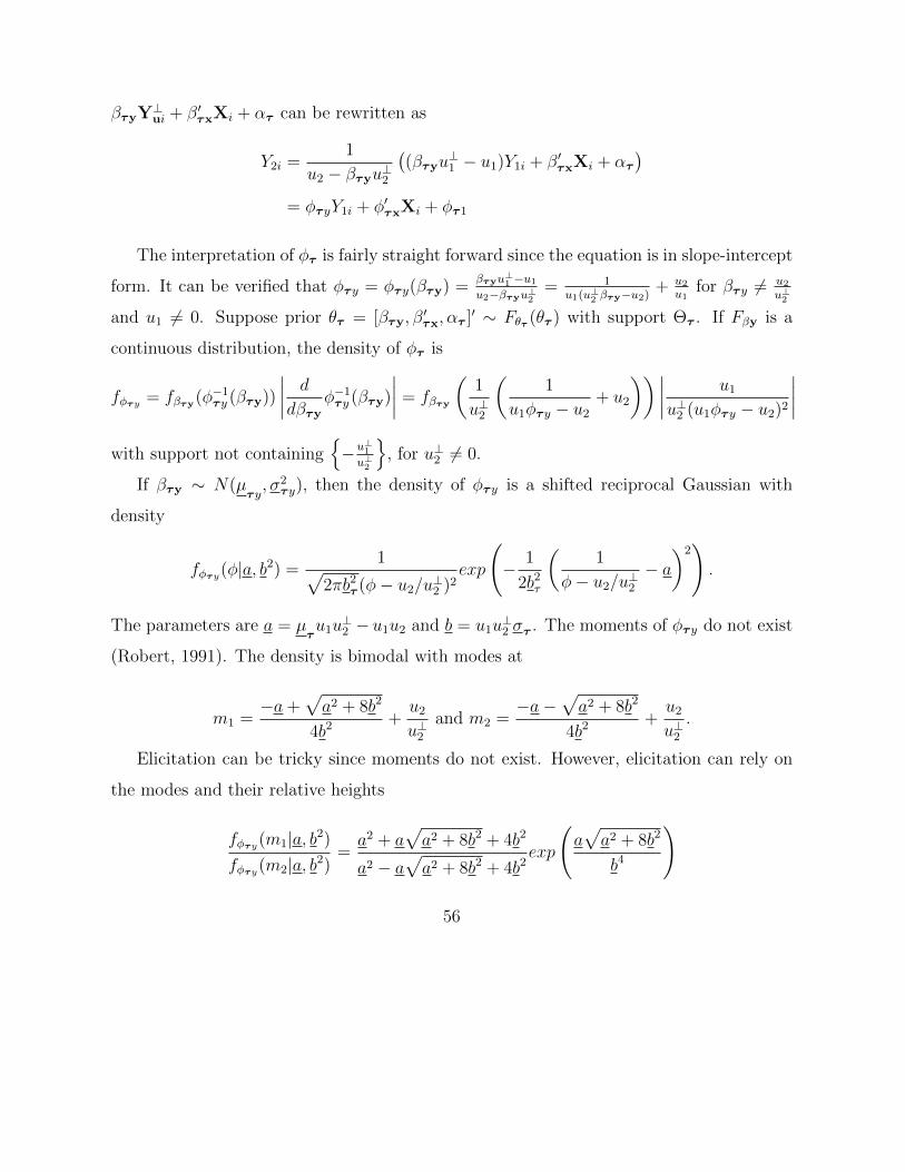
βτyY⊥ui + β′τxXi + ατ can be rewritten as

Y2i =1

u2 − βτyu⊥2

((βτyu

⊥1 − u1)Y1i + β′τxXi + ατ

)= φτyY1i + φ′τxXi + φτ1

The interpretation of φτ is fairly straight forward since the equation is in slope-intercept

form. It can be verified that φτy = φτy(βτy) =βτyu⊥1 −u1

u2−βτyu⊥2= 1

u1(u⊥2 βτy−u2)+ u2

u1for βτy 6= u2

u⊥2

and u1 6= 0. Suppose prior θτ = [βτy, β′τx, ατ ]′ ∼ Fθτ (θτ ) with support Θτ . If Fβy is a

continuous distribution, the density of φτ is

fφτy = fβτy(φ−1τy (βτy))

∣∣∣∣ d

dβτy

φ−1τy (βτy)

∣∣∣∣ = fβτy

(1

u⊥2

(1

u1φτy − u2

+ u2

)) ∣∣∣∣ u1

u⊥2 (u1φτy − u2)2

∣∣∣∣with support not containing

{−u⊥1u⊥2

}, for u⊥2 6= 0.

If βτy ∼ N(µτy, σ2τy), then the density of φτy is a shifted reciprocal Gaussian with

density

fφτy(φ|a, b2) =1√

2πb2τ (φ− u2/u⊥2 )2

exp

(− 1

2b2τ

(1

φ− u2/u⊥2− a)2).

The parameters are a = µτu1u

⊥2 − u1u2 and b = u1u

⊥2 στ . The moments of φτy do not exist

(Robert, 1991). The density is bimodal with modes at

m1 =−a+

√a2 + 8b2

4b2 +u2

u⊥2and m2 =

−a−√a2 + 8b2

4b2 +u2

u⊥2.

Elicitation can be tricky since moments do not exist. However, elicitation can rely on

the modes and their relative heights

fφτy(m1|a, b2)

fφτy(m2|a, b2)=a2 + a

√a2 + 8b2 + 4b2

a2 − a√a2 + 8b2 + 4b2

exp

(a√a2 + 8b2

b4

)

56

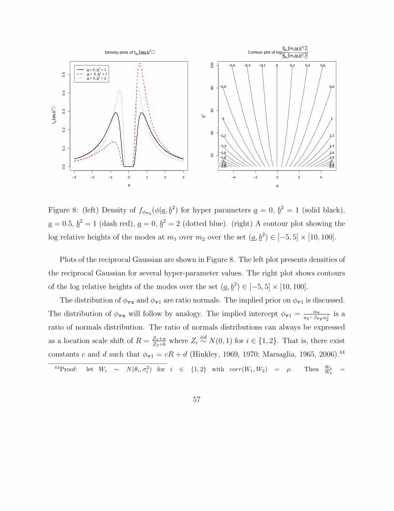
−3 −2 −1 0 1 2 3

0.0

0.1

0.2

0.3

0.4

0.5

Density plots of fφτy(φ|a,b2)

φ

f φτy(φ

|a,b

2 )

a = 0, b2 = 1a = .5, b2 = 1a = 0, b2 = 2

Contour plot of log

fφτy

(m1|a,b2)fφτy

(m2|a,b2)

a

b2

−2.6 −2.4 −2.2 −2

−1.8 −1.6

−1.4

−1.2

−1

−0.8

−0.6 −0.4 −0.2 0 0.2 0.4 0.6

0.8

1

1.2

1.4

1.6 1.8 2

2.2 2.4 2.6

−4 −2 0 2 4

2040

6080

100

Figure 8: (left) Density of fφτy(φ|a, b2) for hyper parameters a = 0, b2 = 1 (solid black),

a = 0.5, b2 = 1 (dash red), a = 0, b2 = 2 (dotted blue). (right) A contour plot showing the

log relative heights of the modes at m1 over m2 over the set (a, b2) ∈ [−5, 5]× [10, 100].

Plots of the reciprocal Gaussian are shown in Figure 8. The left plot presents densities of

the reciprocal Gaussian for several hyper-parameter values. The right plot shows contours

of the log relative heights of the modes over the set (a, b2) ∈ [−5, 5]× [10, 100].

The distribution of φτx and φτ1 are ratio normals. The implied prior on φτ1 is discussed.

The distribution of φτx will follow by analogy. The implied intercept φτ1 = ατ

u2−βτyu⊥2is a

ratio of normals distribution. The ratio of normals distributions can always be expressed

as a location scale shift of R = Z1+aZ2+b

where Ziiid∼ N(0, 1) for i ∈ {1, 2}. That is, there exist

constants c and d such that φτ1 = cR + d (Hinkley, 1969, 1970; Marsaglia, 1965, 2006).44

44Proof: let Wi ∼ N(θi, σ2i ) for i ∈ {1, 2} with corr(W1,W2) = ρ. Then W1

W2=

57

The density of φτ1 is

fφτ1(φ|a, b) =e−

12

(a2+b2)

π(1 + φ2)

[1 + ce

12c2∫ c

0

e−12t2dt

], where c =

b+ aφ√1 + φ2

.

Note, when a = b = 0, then the distribution reduces to the standard Cauchy distribution.

The ratio of normals distribution, like the reciprocal Gaussian distribution, has no moments

and can be bimodal. Focusing on the positive quadrant of (a, b), if a ≤ 1 and b ≥ 0 then

ratio of normals distribution is unimodal. If a & 2.256058904 then the ratio of normals

distribution is bimodal. There is a curve that separates the unimodal and bimodal regions.45

Figure 9 shows three plots for the density of the ratio of normals distribution and the bottom

right plot shows the regions where the density is unimodal and bimodal. The unimodal

region is to the left of the presented curve and the bimodal region is to the right of the

presented curve. If the ratio of normals distribution is bimodal, one mode will be to the

left of −b/a and the other to the right of −b/a. The left mode tends to be much lower than

the right mode for positive (a, b). Unlike the reciprocal Gaussian, closed form solutions for

the modes do not exist. The distribution is approximately elliptical with central tendency

µ = a1.01b−0.2713

and squared dispersion σ2 = a2+1

b2+0.108b−3.795− µ2 when a < 2.256 and 4 < b

(Marsaglia, 2006).

σ1

σ2

√1− ρ2

(θ1σ1

+Z1

θ2σ2

+Z2

+ ρ√1−ρ2

)where Zi ∼ N(0, 1) for i ∈ {1, 2} with corr(Z1, Z2) = 0. Thus a = θ1

σ1,

b = θ2σ2

, c = σ1

σ2

√1− ρ2 and d = c ρ√

1−ρ2where θ1 = aτ1, θ2 = u2 − aτyu⊥2 , σ1 = bτ1 and σ2 = bτyu

⊥2 .

45The curve is approximately b = 18.621−63.411a2−54.668a3+17.716a4−2.2986a52.256058904−a for a ≤ 2.256....

58

−3 −2 −1 0 1 2 3

0.0

0.2

0.4

0.6

0.8

Density plots of fφτ1(φ|a,b) for a

φ

f φτ1(φ

|a,b

)a = 0, b = 0a = 1, b = 0a = 4, b = 0

−3 −2 −1 0 1 2 3

0.0

0.2

0.4

0.6

0.8

Density plots of fφτ1(φ|a,b) for b

φ

f φτ1(φ

|a,b

)

a = 0, b = 0a = 0, b = 1a = 0, b = 2

−3 −2 −1 0 1 2 3

0.0

0.2

0.4

0.6

0.8

Density plots of fφτ1(φ|a,b) for a and b

φ

f φτ1(φ

|a,b

)

a = 0, b = 0a = 1, b = 1a = −1, b = 1a = 2, b = 2

0 1 2 3 4

02

46

810

Modal regions of fφτ1(φ|a,b)

a

bUnimodal Region Bimodal Region

Figure 9: The top two plots and the bottom left plot show the density of the ratio normal

distribution with parameters (a, b). The top left plot shows the density for different values

of a with b fixed at zero. The parameters (a, b) = (1, 0) and (4, 0) result in the same density

as (a, b) = (−1, 0) and (−4, 0). The top right plot shows the density for different values of

b with a fixed at zero. The parameters (a, b) = (0, 1) and (0, 2) result in the same density

as (a, b) = (0,−1) and (0,−2). The bottom left plot shows the density for different values

of a and b. The parameters (a, b) = (1, 1), (−1, 1)and (2, 2) result in the same density as

(a, b) = (−1,−1), (1,−1)and (−2,−2). The bottom right graph shows the regions of the

positive quadrant of the parameter space where the density is either bimodal or unimodal.59

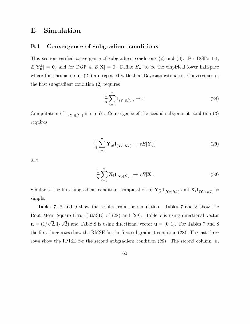
E Simulation

E.1 Convergence of subgradient conditions

This section verified convergence of subgradient conditions (2) and (3). For DGPs 1-4,

E[Y⊥u ] = 02 and for DGP 4, E[X] = 0. Define H−τ to be the empirical lower halfspace

where the parameters in (21) are replaced with their Bayesian estimates. Convergence of

the first subgradient condition (2) requires

1

n

n∑i=1

1(Yi∈H−τ ) → τ. (28)

Computation of 1(Yi∈H−τ ) is simple. Convergence of the second subgradient condition (3)

requires

1

n

n∑i=1

Y⊥ui1(Yi∈H−τ ) → τE[Y⊥u ] (29)

and

1

n

n∑i=1

Xi1(Yi∈H−τ ) → τE[X]. (30)

Similar to the first subgradient condition, computation of Y⊥ui1(Yi∈H−τ ) and Xi1(Yi∈H−τ ) is

simple.

Tables 7, 8 and 9 show the results from the simulation. Tables 7 and 8 show the

Root Mean Square Error (RMSE) of (28) and (29). Table 7 is using directional vector

u = (1/√

2, 1/√

2) and Table 8 is using directional vector u = (0, 1). For Tables 7 and 8

the first three rows show the RMSE for the first subgradient condition (28). The last three

rows show the RMSE for the second subgradient condition (29). The second column, n,

60

is the sample size. The next five columns are the DGPs previously described. It is clear

that as sample size increases the RMSEs are decreasing, showing the convergence of the

subgradient conditions.

Data Generating Process

n 1 2 3 4

102 4.47e-02 2.91e-02 1.52e-02 1.75e-02

Sub Grad 1 103 5.44e-03 4.59e-03 2.48e-03 2.60e-03

104 9.29e-04 8.66e-04 5.42e-04 5.12e-04

102 6.34e-03 1.43e-02 4.34e-02 7.06e-02

Sub Grad 2 103 2.01e-03 3.29e-03 1.32e-02 2.05e-02

104 5.82e-04 8.00e-04 3.59e-03 4.91e-03

Table 7: Unconditional model RMSE of subgradient conditions for u = (1/√

2, 1/√

2)

Table 9 shows RMSE of (30) for the covariate subgradient condition of DGP 4. The

three rows show sample size and the two columns show direction. It is clear that as

sample size increases the RMSEs are decreasing, showing convergence of the subgradient

conditions.

F Application

F.1 Fixed-u hyperplanes

Figure 10 shows fixed-u λτ hyperplanes for various τ along a fixed u direction with model

(9). The values of τ are {0.01, 0.05, 0.1, 0.2, 0.3, 0.4, 0.5, 0.6, 0.7, 0.8, 0.9, 0.95, 0.99}. Two

directions are presented: u = (1/√

2, 1/√

2) (left) and u = (1, 0) (right). The direction

61

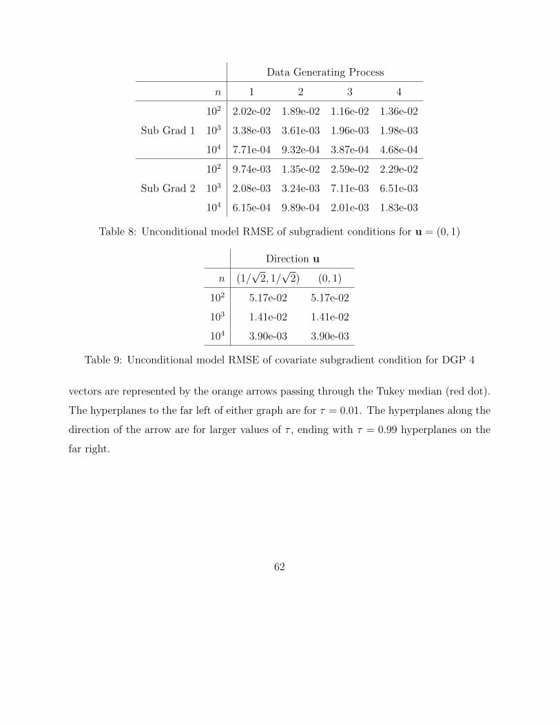
Data Generating Process

n 1 2 3 4

102 2.02e-02 1.89e-02 1.16e-02 1.36e-02

Sub Grad 1 103 3.38e-03 3.61e-03 1.96e-03 1.98e-03

104 7.71e-04 9.32e-04 3.87e-04 4.68e-04

102 9.74e-03 1.35e-02 2.59e-02 2.29e-02

Sub Grad 2 103 2.08e-03 3.24e-03 7.11e-03 6.51e-03

104 6.15e-04 9.89e-04 2.01e-03 1.83e-03

Table 8: Unconditional model RMSE of subgradient conditions for u = (0, 1)

Direction u

n (1/√

2, 1/√

2) (0, 1)

102 5.17e-02 5.17e-02

103 1.41e-02 1.41e-02

104 3.90e-03 3.90e-03

Table 9: Unconditional model RMSE of covariate subgradient condition for DGP 4

vectors are represented by the orange arrows passing through the Tukey median (red dot).

The hyperplanes to the far left of either graph are for τ = 0.01. The hyperplanes along the

direction of the arrow are for larger values of τ , ending with τ = 0.99 hyperplanes on the

far right.

62

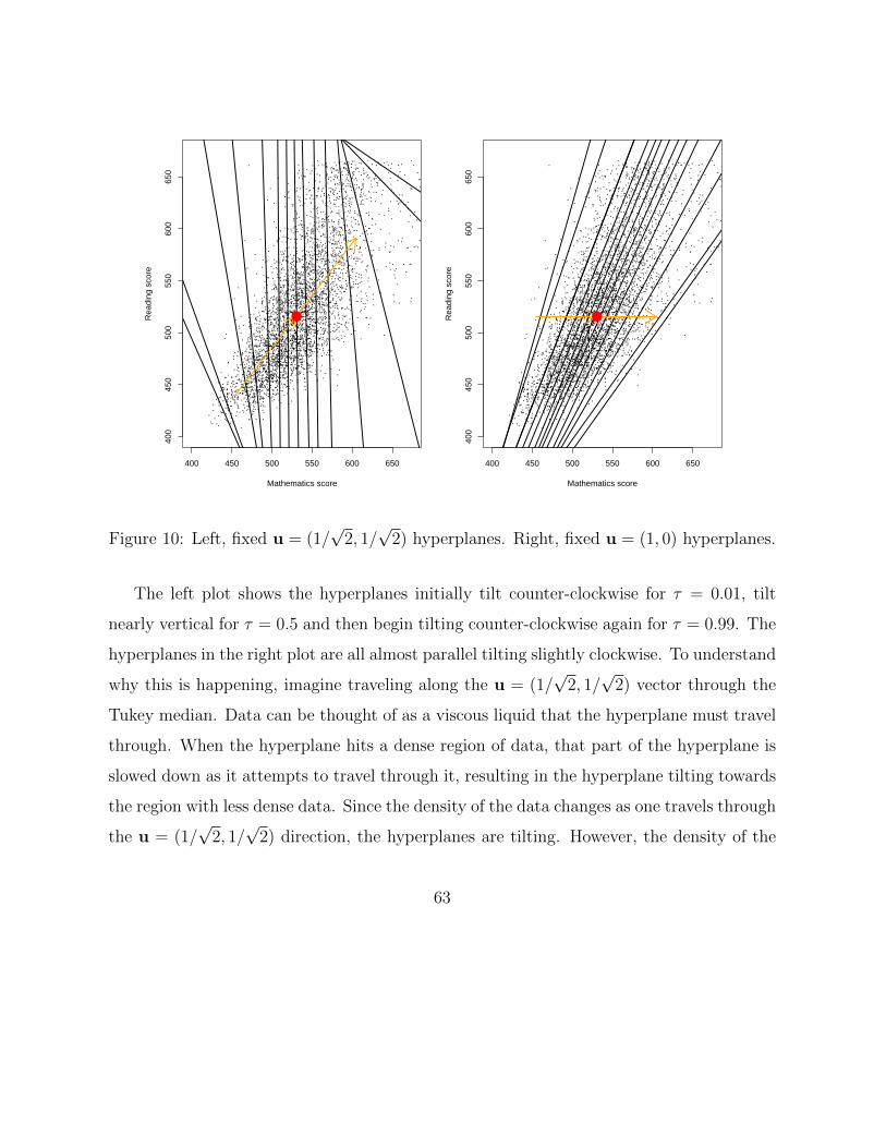
400 450 500 550 600 650

400

450

500

550

600

650

Mathematics score

Rea

ding

sco

re

●

400 450 500 550 600 65040

045

050

055

060

065

0

Mathematics score

Rea

ding

sco

re

●

Figure 10: Left, fixed u = (1/√

2, 1/√

2) hyperplanes. Right, fixed u = (1, 0) hyperplanes.

The left plot shows the hyperplanes initially tilt counter-clockwise for τ = 0.01, tilt

nearly vertical for τ = 0.5 and then begin tilting counter-clockwise again for τ = 0.99. The

hyperplanes in the right plot are all almost parallel tilting slightly clockwise. To understand

why this is happening, imagine traveling along the u = (1/√

2, 1/√

2) vector through the

Tukey median. Data can be thought of as a viscous liquid that the hyperplane must travel

through. When the hyperplane hits a dense region of data, that part of the hyperplane is

slowed down as it attempts to travel through it, resulting in the hyperplane tilting towards

the region with less dense data. Since the density of the data changes as one travels through

the u = (1/√

2, 1/√

2) direction, the hyperplanes are tilting. However, the density of the

63

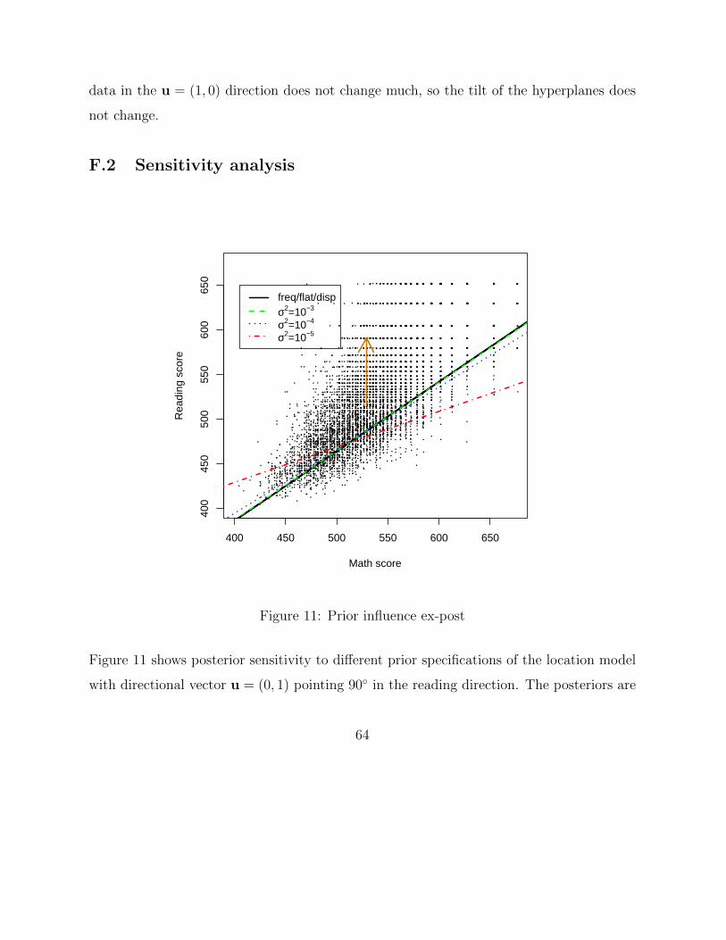
data in the u = (1, 0) direction does not change much, so the tilt of the hyperplanes does

not change.

F.2 Sensitivity analysis

400 450 500 550 600 650

400

450

500

550

600

650

Math score

Rea

ding

sco

re

freq/flat/dispσ2=10−3

σ2=10−4

σ2=10−5

Figure 11: Prior influence ex-post

Figure 11 shows posterior sensitivity to different prior specifications of the location model

with directional vector u = (0, 1) pointing 90◦ in the reading direction. The posteriors are

64

compared against the frequentist estimate (solid black line). The first specification is the

(improper) flat prior (i.e. Lebesgue measure) represented by the solid black line and cannot

be visually differentiated from the frequentist estimate. The rest of the specifications

are proper priors with common mean, µθτ = 02. The dispersed prior has covariance

Σθτ = 1000I2 and is represented by the solid black line and cannot be visually differentiated

from the frequentist estimate or the estimate from the flat prior. The next three priors

have covariance matrices Σθτ = diag(1000, σ2) with σ2 = 10−3 (dashed green), σ2 = 10−4

(dotted blue) and σ2 = 10−5 (dash dotted red). As the prior becomes more informative βτ

converges to zero with resulting model ˆreadingi = ατ .

References

Alhamzawi, R., K. Yu, and D. F. Benoit (2012). Bayesian adaptive lasso quantile regression.

Statistical Modelling 12 (3), 279–297.

Benoit, D. F. and D. Van den Poel (2012). Binary quantile regression: a Bayesian approach

based on the asymmetric Laplace distribution. Journal of Applied Econometrics 27 (7),

1174–1188.

Benoit, D. F. and D. Van den Poel (2017). bayesQR: A Bayesian approach to quantile

regression. Journal of Statistical Software 76 (7), 1–32.

Chernozhukov, V. and H. Hong (2003). An MCMC approach to classical estimation. Jour-

nal of Econometrics 115 (2), 293–346.

Dagpunar, J. (1989). An easily implemented generalised inverse Gaussian generator. Com-

munications in Statistics - Simulation and Computation 18 (2), 703–710.

65

Drovandi, C. C. and A. N. Pettitt (2011). Likelihood-free Bayesian estimation of multivari-

ate quantile distributions. Computational Statistics & Data Analysis 55 (9), 2541–2556.

Dutta, S., A. K. Ghosh, P. Chaudhuri, et al. (2011). Some intriguing properties of Tukeys

half-space depth. Bernoulli 17 (4), 1420–1434.

Embrechts, P. and M. Hofert (2013). A note on generalized inverses. Mathematical Methods

of Operations Research 77 (3), 423–432.

Feng, C., H. Wang, X. M. Tu, and J. Kowalski (2012). A note on generalized inverses of

distribution function and quantile transformation. Applied Mathematics 3 (12A), 2098–

2100.

Feng, Y., Y. Chen, and X. He (2015). Bayesian quantile regression with approximate

likelihood. Bernoulli 21 (2), 832–850.

Finn, J. D. and C. M. Achilles (1990). Answers and questions about class size: A statewide

experiment. American Educational Research Journal 27 (3), 557–577.

Folger, J. and C. Breda (1989). Evidence from project star about class size and student

achievement. Peabody Journal of Education 67 (1), 17–33.

Fox, M. and H. Rubin (1964, September). Admissibility of quantile estimates of a single

location parameter. Ann. Math. Statist. 35 (3), 1019–1030.

Hallin, M., Z. Lu, D. Paindaveine, and M. iman (2015, 08). Local bilinear multiple-output

quantile/depth regression. Bernoulli 21 (3), 1435–1466.

Hallin, M., D. Paindaveine, and M. Siman (2010). Multivariate quantiles and multiple-

output regression quantiles: from L1 optimization to halfspace depth. The Annals of

Statistics 38 (2), 635–703.

66

Hastings, W. K. (1970, 04). Monte Carlo sampling methods using Markov chains and their

applications. Biometrika 57 (1), 97–109.

Hinkley, D. V. (1969). On the ratio of two correlated normal random variables.

Biometrika 56 (3), 635–639.

Hinkley, D. V. (1970). Correction: ‘on the ratio of two correlated normal random variables’.

Biometrika 57 (3), 683.

Khare, K. and J. P. Hobert (2012). Geometric ergodicity of the Gibbs sampler for Bayesian

quantile regression. Journal of Multivariate Analysis 112, 108 – 116.

Kleijn, B. J. and A. W. van der Vaart (2006). Misspecification in infinite-dimensional

Bayesian statistics. The Annals of Statistics 38 (2), 837–877.

Koenker, R. (2005). Quantile Regression. Econometric Society Monographs. Cambridge

University Press.

Koenker, R. (2018). quantreg: Quantile Regression. R package version 5.38.

Koenker, R. and G. Bassett (1978). Regression quantiles. Econometrica: Journal of the

Econometric Society 38 (1), 33–50.

Kong, L. and I. Mizera (2012). Quantile tomography: using quantiles with multivariate

data. Statistica Sinica 22 (4), 1589–1610.

Kottas, A. and M. Krnjajic (2009). Bayesian semiparametric modelling in quantile regres-

sion. Scandinavian Journal of Statistics 36 (2), 297–319.

67

Kotz, S., T. Kozubowski, and K. Podgorski (2001). The Laplace Distribution and General-

izations: A Revisit with Applications to Communications, Economics, Engineering, and

Finance. Progress in Mathematics Series. Birkhauser Boston.

Kozumi, H. and G. Kobayashi (2011). Gibbs sampling methods for Bayesian quantile

regression. Journal of Statistical Computation and Simulation 81 (11), 1565–1578.

Krueger, A. B. (1999). Experimental estimates of education production functions. The

Quarterly Journal of Economics 114 (2), 497–532.

Laine, B. (2001). Depth contours as multivariate quantiles: A directional approach. Mas-

ter’s thesis, Univ. Libre de Bruxelles, Brussels.

Lancaster, T. and S. Jae Jun (2010). Bayesian quantile regression methods. Journal of

Applied Econometrics 25 (2), 287–307.

Li, Q., R. Xi, N. Lin, et al. (2010). Bayesian regularized quantile regression. Bayesian

Analysis 5 (3), 533–556.

Liu, J. S. (2008). Monte Carlo strategies in scientific computing. Springer Science &

Business Media.

Marsaglia, G. (1965). Ratios of normal variables and ratios of sums of uniform variables.

Journal of the American Statistical Association 60 (309), 193–204.

Marsaglia, G. (2006, May). Ratios of normal variables. Journal of Statistical Software 16,

1–10.

McKeague, I. W., S. Lopez-Pintado, M. Hallin, and M. Siman (2011). Analyzing growth

trajectories. Journal of Developmental Origins of Health and Disease 2 (6), 322329.

68

Mosteller, F. (1995). The Tennessee study of class size in the early school grades. The

future of children 5 (2), 113–127.

Neal, R. M. (2003, 06). Slice sampling. Ann. Statist. 31 (3), 705–767.

Paindaveine, D. and M. Siman (2011). On directional multiple-output quantile regression.

Journal of Multivariate Analysis 102 (2), 193 – 212.

Rahman, M. A. (2016). Bayesian quantile regression for ordinal models. Bayesian Analy-

sis 11 (1), 1–24.

Rahman, M. A. and S. Karnawat (2019, 09). Flexible Bayesian quantile regression in

ordinal models. Advances in Econometrics 40B, 211–251.

Rice, J. K. (2010). The impact of teacher experience: Examining the evidence and policy

implications. brief no. 11. Technical report.

Robert, C. (1991). Generalized inverse normal distributions. Statistics & Probability Let-

ters 11 (1), 37–41.

Rousseeuw, P. J. and I. Ruts (1999). The depth function of a population distribution.

Metrika 49 (3), 213–244.

Serfling, R. (2002). Quantile functions for multivariate analysis: approaches and applica-

tions. Statistica Neerlandica 56 (2), 214–232.

Serfling, R. and Y. Zuo (2010, 04). Discussion. Ann. Statist. 38 (2), 676–684.

Small, C. G. (1990). A survey of multidimensional medians. International Statistical Review

/ Revue Internationale de Statistique 58 (3), 263–277.

69

Sriram, K. (2015). A sandwich likelihood correction for Bayesian quantile regression based

on the misspecified asymmetric Laplace density. Statistics & Probability Letters 107, 18

– 26.

Sriram, K., R. Ramamoorthi, P. Ghosh, et al. (2013). Posterior consistency of Bayesian

quantile regression based on the misspecified asymmetric Laplace density. Bayesian

Analysis 8 (2), 479–504.

Sriram, K., R. V. Ramamoorthi, and P. Ghosh (2016). On Bayesian quantile regression

using a pseudo-joint asymmetric Laplace likelihood. Sankhya A 78 (1), 87–104.

Taddy, M. A. and A. Kottas (2010). A Bayesian nonparametric approach to inference for

quantile regression. Journal of Business & Economic Statistics 28 (3), 357–369.

Tanner, M. and W. Wong (1987). The calculation of posterior distributions by data aug-

mentation. Journal of the American Statistical Association 82 (398), 528–540.

Thompson, P., Y. Cai, R. Moyeed, D. Reeve, and J. Stander (2010). Bayesian nonparamet-

ric quantile regression using splines. Computational Statistics & Data Analysis 54 (4),

1138–1150.

Tukey, J. W. (1975). Mathematics and the picturing of data.

Waldmann, E. and T. Kneib (2014). Bayesian bivariate quantile regression. Statistical

Modelling 15 (4), 326–344.

Wang, H. J. and Y. Yang (2016). AdjBQR: Adjusted Bayesian Quantile Regression Infer-

ence. R package version 1.0.

70

Word, E., J. Johnston, H. P. Bain, B. D. Fulton, J. B. Zaharias, C. M. Achilles, M. N. Lintz,

J. Folger, and C. Breda (1990). The state of Tennessee’s student/teacher achievement

ratio (star) project: Technical report 1985 – 1990. Technical report, Tennessee State

Department of Education.

Yang, Y., H. J. Wang, and X. He (2015). Posterior inference in Bayesian quantile regression

with asymmetric Laplace likelihood. International Statistical Review 84 (3), 327–344.

10.1111/insr.12114.

Yu, K., Z. Lu, and J. Stander (2003). Quantile regression: applications and current research

areas. Journal of the Royal Statistical Society: Series D (The Statistician) 52 (3), 331–

350.

Yu, K. and R. A. Moyeed (2001). Bayesian quantile regression. Statistics & Probability

Letters 54 (4), 437–447.

Zscheischler, J. (2014). A global analysis of extreme events and consequences for the ter-

restrial carbon cycle. Ph. D. thesis, ETH Zurich.

71