A case study to estimate design effort for Pratt \u0026 Whitney canada

$Page 1: A case study to estimate design effort for Pratt \u0026 Whitney canada$
ISSN 1750-9653, England, UKInternational Journal of Management Science

and Engineering ManagementVol. 3 (2008) No. 4, pp. 284-293

A case study to estimate design effort for Pratt & Whitney canada ∗

Adil M. Salam1†, Nadia F. Bhuiyan1, Gerard J. Gouw1, Syed Asif Raza2

1 Department of Mechanical and Industrial Engineering, Concordia University, Montreal, Canada2 Centre de recherche sur les transports, Universitede Montreal, Montreal, Canada

(Received December 25 2007, Accepted March 10 2008)

Abstract. The design effort required to complete a project is an important aspect of a project. It impactsthe final cost, as well as the lead-time of a project. In this paper, a case study, which is carried out at Pratt &Whitney Canada, a global leader in the design and manufacture of aircraft engines, is presented. A Parametricmodel is proposed to estimate the design effort required in for a particular department to complete their designphase of an integrated blade-rotor low-pressure compressor fan. In a sensitivity analysis, the model estimationis compared with the actual estimates and the comparison demonstrates that the parametric model results ina good estimation. The analysis further explores the impact of various factors used to develop the parametricmodel, as well as demonstrates the significance of the proposed modeling methodology.

Keywords: design effort, parametric model, estimation, sensitivity analysis

1 Introduction

The primary issues in a project are the lead-time and the cost it may require. To accurately estimate thetime required to complete a project would resolve a lot of problems related to forecasting, scheduling, biddingand reputation. Even though, there have been studies to control a project according to plan (Thamhain andWilemon, 1986; Grant et al., 2006)[10, 22], there exists a need to further investigate this matter. A case studyconducted by Bounds (1998)[5], stated that only 26% percent of the projects completed in the US were on timeand within budget.

Frimpong (2000)[9] found that only 25% of construction projects were within budget and completed ontime. Assaf and Al-Hejji (2006)[1] conducted a survey and found that only 30% of the construction projectswere completed on time. The delays for the projects ranged from 10-30%. Moreover, the research of Norris(1971)[19] and of Murmann (1994)[18] pointed out that the unexpected or underestimated cost of projects wasbetween 97-151% more than the original estimate. It is even more drastic in schedule, running from 41-258%later than originally estimated.

According to Bronikowski (1986)[6] these inaccurate estimates would sometimes lead to the terminationof projects resulting in the company incurring huge costs and waste of effort of their resources. If a newproduct is being launched, time to market is critical. According to Ulrich and Eppinger (2003)[23], missingthe target schedule could result in failing to launch the new product with competitors taking control of themarket. There are several studies reported in the literature that show that the underestimation of design effortis a major cause of delays and budget cost errors (Colmer et al., 1999; Bashir and Thomson, 2004)[3, 7].

Colmer et al. (1999)[7] studied design effort and costing improvement issues in a new product develop-ment project. There paper presented a discussion on why these new projects are vulnerable to cost overruns.

∗ The authors are indebted to Mr. Yvan Beauregard from Pratt & Whitney Canada for his support and assistance towards thisresearch.

† Corresponding author. E-mail address: a [email protected].

Published by World Academic Press, World Academic Union

International Journal of Management Science and Engineering Management, Vol. 3 (2008) No. 4, pp. 284-293 285

They discussed how the limitations of cost estimates lead to poor decision making, which contributes to costand schedule overruns. They discussed some issues regarding project and risk management, which will helpprojects meet their own needs and the need of the customers.

Bashir and Thomson (1999)[2] developed a model to estimate design effort based on the product com-plexity (PC). PC was assumed to be a metric that depends on the number of functions and the depth of theirfunctional trees. Later, Bashir and Thomson (2004)[3] analyzed fifteen designs and developed a parametricmodel to estimate the time required to design hydroelectric generators for General Electric.

The work presented in this paper extends the studies carried out in Bashir and Thomson (2004)[3]. Themodel presented in this research is also parametric, however; the work presented in paper differs from anearlier study presented in Bashir and Thomson (2004)[3] since it is a case study which is specialized foraerodynamic department at Pratt and Whitney Canada (PWC). In order to develop parametric model for theestimation of the design effort in an integrated blade-rotor low-pressure compressor fan manufacturing processat the department. New factors specific to aerodynamic department at PWC are identified that are used in theproposed parametric model, which contribute to improve the design effort estimation. Bashir and Thomson(2004)[3] proposed a generalized parametric model for estimating design effort for different project and thusused common factors such as product complexity (PC). PC remains the same for a single type of product,thus it is not considered in the case study specific to a single type of product development process at particulardepartment at PWC. Next, we propose a parametric model to estimate the design effort for an integrated blade-rotor low-pressure compressor (IBR LPC) fan designed and manufactured at PWC. The company is interestedin quantifying the design effort of various departments for engine components.

The rest of the paper is organized as follows: Section 2 presents the model of design effort estimation,including a discussion of the prominent factors that are used in parametric modeling, followed by an overviewof the jackknife and data masking techniques utilized in the modeling. Section 3, presents the use of mul-tiple linear regression (MLR) method to analyzed aforementioned parametric model. The outcomes of theMLR based analysis is reported in section 4. Finally, the conclusions and suggestions for future research areidentified in section 5.

2 Design effort estimation for the aerodynamics department

In this section, a parametric modeling approach is presented. The proposed model enables estimation ofthe effort measured in human-hours required to design an IBR LPC fan in aerodynamic department at PWC.The data information used in the model development and analysis is from aerodynamic department PWC. Inorder to maintain the confidentiality of the equipment manufacturer’s information, the engines of the compres-sor fans being studied will not be disclosed. Furthermore, the actual data received from PWC are masked usingthe general additive data perturbation (GADP) method suggested in Muralidhar et al. (1999)[17]. The GADPmethod maintains the characteristics of the attributes of the original data in terms of linear combinations andthe correlation of factors while using the masked values for these attributes. Among the other essentially im-portant features of the GADP method is that it is free from several types of biases and maintains security ofthe masked attributes.

Bashir and Thomson (2004)’s work suggested a parametric model built using the data for design timerecorded for hydro projects at General Electric. Equation (1) states parametric model for estimating designeffort used in the work. The model involves several factors that are believed to be the significant factors alongwith the product complexity (PC) factor.

E = aPCbDc11 Dc2

2 . . . Dcmm (1)

where,E: Estimated design effort in hoursPC: Product complexityDm: Effort driver (factor m)a, b, cm, Constants (weights) estimated from historical data

MSEM email for subscription: [email protected]

286 A. Salam & N. Bhuiyan & et al.: A case study to estimate design effort

This research presents methodology to use the parametric modeling dedicated to the estimation of thedesign effort for IBR LPC fan in aerodynamic department at PWC. Whereas an earlier model suggested inBashir and Thomson (2004)[3] uses PC as a driver of effort, it is omitted in this work because this model isdeveloped solely to a specific type of component in the same engine family for PWC; hence product complex-ity is not a factor. It is also expected a model specific to a department would improve estimation capabilityand would also give better understanding about the department from the parametric model. The proposedparametric model is shown in equation (2):

E = a0Da11 Da2

2 . . . DamM (2)

The design effort estimation model was developed using data provided on seven specific design jobs (DJs)by PWC for the IBR LPC fan for a certain class of turbo fan engines. It was essential to identify the principaldesign parameters (factors) that may have significant impact on the design effort estimation. After holdingseveral interviews and discussions with managers, designers, and project engineers at PWC, the followingfour factors, listed below, were selected as the parameters to be used in this study:

• Type of design (TD)• Degree of change (DC)• Concurrency (Con)• Experience of departmental personnel (DE)

2.1 Type of design

When designing a component, the effort required to complete the will highly depend on the type ofdesign (TD). An initial design is not usually expected to require the same amount of time as a redesign. Forthis reason, each DJ was assigned one of the following attributes:

• Initial Design: 1• Redesign: 2

2.2 Degree of change

Another factor considered to be of importance was the degree of change (DC). The purpose of this factoris used to attribute a value to the level of rework created from the initial design to a redesign, or from a redesignto a subsequent redesign. Supposing there is a major change to a given design, the amount of rework generatedwould be expected to be greater than if only a minor design change is required. In fact, as will be seen in thedata, in some cases, a major change resulted in more effort than the initial design. Thus, different values wereattributed to the designs as shown below:

• Initial design: 1• Redesign with minor modifications: 2• Redesign with major modifications: 3

2.3 Concurrency

It is noticed that product development teams practice concurrent engineering (CE) at PWC. The impactof CE in reducing the lead time is well established in the works of many research such as Loch and Terwiesch(1998)[14], Yassine et al. (1999)[26], Joglekar et al. (2001)[11], Yassine and Braha (2003)[25], Bhuiyan et al.(2004)[4] that CE reduces the overall lead-time to design components. On the other hand, it is equally importantto understand the level or amount of concurrency involved in the design, because it has also been pointed outby numerous researchers such as Bhuiyan et al. (2004)[4], Wang and Yan (2005)[24], and Jun et al. (2005)[12]

that CE tends to create rework, which could add to the total effort required to complete the design of thecomponent. Thus concurrency of activities was considered an important factor and was in turn included inthe model. The concurrency values for each of seven design jobs (A to G) under study are estimated. To

MSEM email for contribution: [email protected]


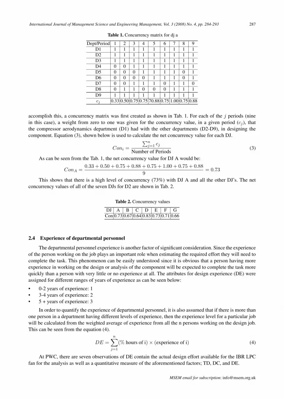
Table 1. Concurrency matrix for dj a

Dept/Period 1 2 3 4 5 6 7 8 9D1 1 1 1 1 1 1 1 1 1D2 1 1 1 1 1 1 1 1 1D3 1 1 1 1 1 1 1 1 1D4 0 0 1 1 1 1 1 1 1D5 0 0 0 1 1 1 1 0 1D6 0 0 0 0 1 1 1 0 1D7 0 0 1 1 1 0 1 1 0D8 0 1 1 0 0 0 1 1 1D9 1 1 1 1 1 1 1 1 1cj 0.33 0.50 0.75 0.75 70.88 0.75 1.00 0.75 0.88

accomplish this, a concurrency matrix was first created as shown in Tab. 1. For each of the j periods (ninein this case), a weight from zero to one was given for the concurrency value, in a given period (cj), thatthe compressor aerodynamics department (D1) had with the other departments (D2-D9), in designing thecomponent. Equation (3), shown below is used to calculate the net concurrency value for each DJ.

Coni =

∑nj=1 cj

Number of Periods(3)

As can be seen from the Tab. 1, the net concurrency value for DJ A would be:

ConA =0.33 + 0.50 + 0.75 + 0.88 + 0.75 + 1.00 + 0.75 + 0.88

9= 0.73

This shows that there is a high level of concurrency (73%) with DJ A and all the other DJ’s. The netconcurrency values of all of the seven DJs for D2 are shown in Tab. 2.

Table 2. Concurrency values

DJ A B C D E F GCon 0.73 0.67 0.64 0.83 0.73 0.71 0.66

2.4 Experience of departmental personnel

The departmental personnel experience is another factor of significant consideration. Since the experienceof the person working on the job plays an important role when estimating the required effort they will need tocomplete the task. This phenomenon can be easily understood since it is obvious that a person having moreexperience in working on the design or analysis of the component will be expected to complete the task morequickly than a person with very little or no experience at all. The attributes for design experience (DE) wereassigned for different ranges of years of experience as can be seen below:

• 0-2 years of experience: 1• 3-4 years of experience: 2• 5 + years of experience: 3

In order to quantify the experience of departmental personnel, it is also assumed that if there is more thanone person in a department having different levels of experience, then the experience level for a particular jobwill be calculated from the weighted average of experience from all the n persons working on the design job.This can be seen from the equation (4).

DE =n∑

j=1

(% hours of i)× (experience of i) (4)

At PWC, there are seven observations of DE contain the actual design effort available for the IBR LPCfan for the analysis as well as a quantitative measure of the aforementioned factors; TD, DC, and DE.



2.5 Parametric modeling

The suggested parametric modeling approach uses multiple linear regression (MLR) technique for theestimation of design effort. Due to the scarcity of the data, the jackknife technique is also utilized with theMLR. This technique is commonly used not only to improve the problem of biased estimation due to smallsample size, but also in situations where the distribution of the data is hard to analyze (Efron and Tibshirani1993)[8]. In principal this technique is based on sub-sampling rule in which the data are divided into sub-samples, and the sub-samples are obtained by deleting one observation at a time. The calculations are carriedout for each sub sample. In a data set x = (x1, x2, x3, . . . , xn), the ith jackknife sample x−i is defined to bex with the ith data point removed. The pseudo-values, Psi , are determined using equation (5).

Psi = nsβ − (ns− 1) ˆβ−i (5)

where,Psi : Pseudo-value for the entire sample, omitting sub-sample i.ns: Number of sub-samplesβ: Least-squares estimator of the whole sampleˆβ−i: Least-squares estimator for the entire sample, omitting sub sample i

The jackknife estimator β is determined as follows with equation (6).

β =∑ns

i=1 Psi

ns(6)

Furthermore to the jackknife technique, GAPD model proposed in Muralidhar et al. (1999)[17] was alsoconsidered in this study to mask the confidential data used in the parametric model.

3 Parametric model analysis

Data was gathered from PWC for the seven DJs. The values for TD, DC, DE and the actual value (ACT)can be seen in Tab. 3.

Table 3. Values for all djs

DJ TD DC Con DE ACTA 1 1 0.73 3.00 182.45B 2 2 0.67 2.80 784.87C 2 3 0.64 3.00 825.71D 1 1 0.83 2.00 218.56E 2 2 0.73 2.07 816.78F 2 3 0.71 2.43 864.88G 1 1 0.66 1.70 228.07

As discussed earlier, the GAPD model of Muralidhar et al. (1999)[17] was used to mask the confidentialattribute, in this case the data on design effort (referred as ACT) measured in person-hours. Thus, wheneverthe term ACT is used in this paper, it refers to the masked values of actual design effort. It is also importantto mention that this analysis was carried out on four departments at PWC. However, the analysis for onlythe compressor aerodynamics department is presented in this paper. The analysis details with the rest of thedepartments can be found in Salam (2007)[21].

The linearization of the proposed parametric model comprised of aforementioned factors. The lineariza-tion enables the use of MLR technique and resulting model is presented in Equation (7). The parametricproposed model is similar to the model suggested in Bashir and Thomson (2004)[3], however, with distinctfactors to estimate the design effort.



ln E = ln(a0) + a1 ln(TD) + a2 ln(DC) + a3 ln(Con) + a4 ln(DE) (7)

The jackknife technique (Efron and Tibshirani, 1993)[8] is used and sub-samples of the data are generated.The technique estimates the jackknife regression coefficients (COEFJACK) associated with each factor andthese are reported in Tab. 4:

Table 4. Regression coefficients

Constants All JackA JackB JackC JackD JackE JackF JackG COEFJACK

ln(a0) 5.583 5.504 5.644 5.598 5.428 5.644 5.598 5.605 5.575a1 1.762 1.727 1.604 1.789 1.814 1.908 1.732 1.690 1.752a2 0.223 0.180 0.339 0.200 0.191 0.147 0.257 0.231 0.221a3 -0.063 -0.050 0.023 -0.035 -0.401 0.023 -0.035 -0.441 -0.131a4 -0.337 -0.180 -0.383 -0.346 -0.315 -0.383 -0.346 -0.466 -0.345

From the jackknife values above, the predicted (PRED) ln of ACT (actual masked values) would be asfollows:

PRED ln(ACT ) = 10.36− 3.361× ln(TD) + 2.112× ln(DC)− 0.955× ln(Con)− 4.972× ln(DE)

An essential assumption in the use of MLR is linearity. As discussed in Kutner et al. (2005)[13], we carried outtwo tests in order to validate the linearity assumption. The first test of linearity was carried out by generatingthe scattered plot of the standardized residuals against the predicted values for the regression, which can beseen as Fig. 1.

Fig. 1. Standardized residual plot

Fig. 1 shows that the standardized residual values fall within the±1 threshold, and there are no curvilinearpatterns, indicating a normal linear behavior. The residual plots were generated for all of the seven jackknifesamples and they also behaved in a similar manner. The second test to be carried out is the normality of errortest. The test requires the value of r, which is the coefficient of correlation. The value of r is calculated fromequation (8).

r = ±√

R2 (8)

The r-value has to be less than the critical value, rL of 0.898 (Looney and Gulledge, 1985)[15]. Thecoefficient of determination, R2 values of the entire sample and all jackknife samples were calculated. Ther-value was calculated from the minimum R2 value, assuming if it passes the test in the worst case, it wouldpass in the rest of the cases. The r-value calculated was 0.999, greater than rL showing normal behavior of



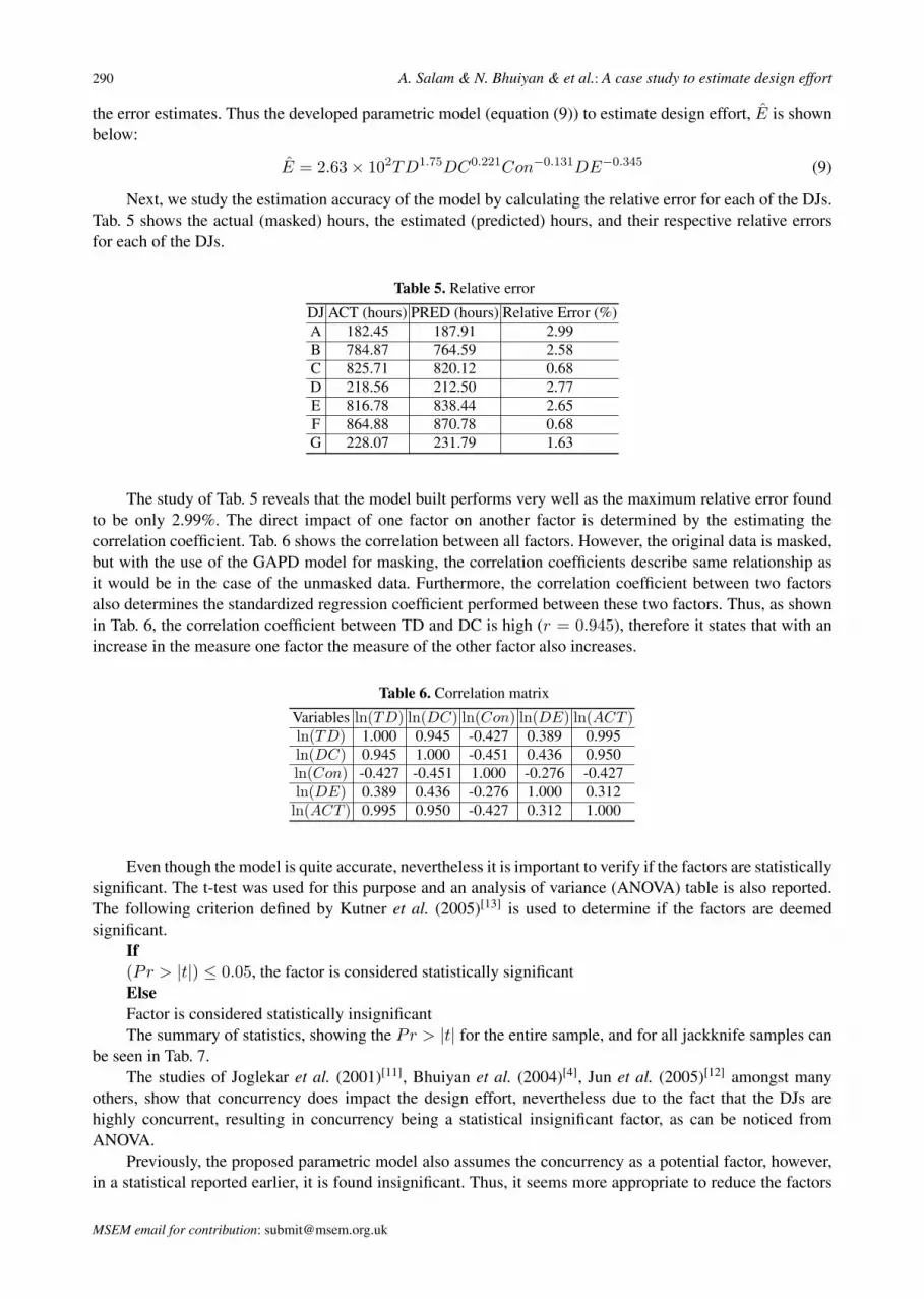
the error estimates. Thus the developed parametric model (equation (9)) to estimate design effort, E is shownbelow:

E = 2.63× 102TD1.75DC0.221Con−0.131DE−0.345 (9)

Next, we study the estimation accuracy of the model by calculating the relative error for each of the DJs.Tab. 5 shows the actual (masked) hours, the estimated (predicted) hours, and their respective relative errorsfor each of the DJs.

Table 5. Relative error

DJ ACT (hours) PRED (hours) Relative Error (%)A 182.45 187.91 2.99B 784.87 764.59 2.58C 825.71 820.12 0.68D 218.56 212.50 2.77E 816.78 838.44 2.65F 864.88 870.78 0.68G 228.07 231.79 1.63

The study of Tab. 5 reveals that the model built performs very well as the maximum relative error foundto be only 2.99%. The direct impact of one factor on another factor is determined by the estimating thecorrelation coefficient. Tab. 6 shows the correlation between all factors. However, the original data is masked,but with the use of the GAPD model for masking, the correlation coefficients describe same relationship asit would be in the case of the unmasked data. Furthermore, the correlation coefficient between two factorsalso determines the standardized regression coefficient performed between these two factors. Thus, as shownin Tab. 6, the correlation coefficient between TD and DC is high (r = 0.945), therefore it states that with anincrease in the measure one factor the measure of the other factor also increases.

Table 6. Correlation matrix

Variables ln(TD) ln(DC) ln(Con) ln(DE) ln(ACT )ln(TD) 1.000 0.945 -0.427 0.389 0.995ln(DC) 0.945 1.000 -0.451 0.436 0.950ln(Con) -0.427 -0.451 1.000 -0.276 -0.427ln(DE) 0.389 0.436 -0.276 1.000 0.312ln(ACT ) 0.995 0.950 -0.427 0.312 1.000

Even though the model is quite accurate, nevertheless it is important to verify if the factors are statisticallysignificant. The t-test was used for this purpose and an analysis of variance (ANOVA) table is also reported.The following criterion defined by Kutner et al. (2005)[13] is used to determine if the factors are deemedsignificant.

If(Pr > |t|) ≤ 0.05, the factor is considered statistically significantElseFactor is considered statistically insignificantThe summary of statistics, showing the Pr > |t| for the entire sample, and for all jackknife samples can

be seen in Tab. 7.The studies of Joglekar et al. (2001)[11], Bhuiyan et al. (2004)[4], Jun et al. (2005)[12] amongst many

others, show that concurrency does impact the design effort, nevertheless due to the fact that the DJs arehighly concurrent, resulting in concurrency being a statistical insignificant factor, as can be noticed fromANOVA.

Previously, the proposed parametric model also assumes the concurrency as a potential factor, however,in a statistical reported earlier, it is found insignificant. Thus, it seems more appropriate to reduce the factors



Table 7. Anova to determine significant factors

Factor All JackA JackB JackC JackD JackE JackF JackG

ln(a0) 0.000 0.004 0.009 0.015 0.008 0.009 0.015 0.023ln(TD) 0.006 0.015 0.058 0.074 0.023 0.047 0.078 0.196ln(DC) 0.157 0.110 0.197 0.436 0.161 0.357 0.396 0.368ln(Con) 0.788 0.568 0.913 0.927 0.236 0.913 0.927 0.895ln(DE) 0.053 0.144 0.114 0.205 0.079 0.114 0.205 0.699

by excluding the concurrency and to reconstruct the model with the remaining factors. The new model is alsosubjected to statistical testing and has successfully passed aforementioned tests suggested for model valida-tion. The new parametric model is reported in equation (10) which estimates design effort for the aerodynamicdepartment at PWC is as follows:

ENo Con = 2.69× 102TD−1.76DC0.225DE−0.325 (10)

Furthermore, the error remained minimal at a maximum value of 3.30%, while using the model reported inequation (10).

4 Sensitivity analysis

In this section, we report a sensitivity analysis to show the main effect of an individual factor’s contribu-tion on the design effort. The results are reported in Fig. 2 ∼ 4:

Fig. 2. Impact of the type of design on design effort

From Fig. 2, it can be seen that if the design were an initial one, it would take longer than that of aredesign. Fig. 3 identifies that the degree of change being major will require more time than a minor one.Finally, Fig. 4 shows that the higher the net level of experience of the departmental personnel working on thedesign job, the less effort is required.

5 Conclusions and future research suggestions

The importance of determining design effort is essential to estimate the lead-time, cost, and manpowerneeded. The product development process is a very complex process and it is dependent on many factorsinvolved in the design process. Even though it is complicated to estimate the design effort needed for thedevelopment of a product, it is essential for the concerned personnel to know it precisely.

Depending upon the product complexity and development strategies, a list of potential factors can beidentified that can help to improve such estimations. In this thesis, a case study focusing on four departments



Fig. 3. Impact of the degree of change on design effort

Fig. 4. Impact of the experience of departmental expertise on design effort

(design, aerodynamics, analytical and drafting) at PWC is presented to estimate the design effort of the inte-grated blade-rotor low- pressure compressor fans.

The study utilizes a parametric modeling technique to estimate the design effort for each of the four de-partments. Four design factors are considered: type of design, degree of change, concurrency, and experienceof departmental personnel. An analysis of each department initially considers all the above-mentioned factorsand reduces to keep only the statistically significant factors. Since the data used in this thesis is confidential,coming from a leading aerospace company, an appropriate method for data masking was required.

The model performed well according to a number of accuracy tests suggested in this paper. Comparisonof the design effort estimation determined by the model is made with the actual design effort reported by PWCfor the each of the seven design jobs. The maximum error observed was 3.30%.

Even though the model has promising results there are limitations to this model. Even though the method-ology can be used for other major components such as the turbine or combustor, the model is specific to theIBR LPC fans for a certain class of engines. Using this approach models will have to be developed for eachtype of component. Also, factors will have to be selected and validated for each type of component. Eventhough the factors are general, there may be other factors that will be relevant to other components beingstudied.

There can be several future applications of this thesis. As mentioned in the limitations, the model is spe-cific to the component, other models can be developed which can be applied not limiting itself to a particulartype of component or class of engine, rather the model can be more general. Another possible applicationcould be to study the length of time (lead-time) to design the components. Knowing the lead-time and phasingof hours will significantly help management in scheduling their tasks and in assigning priorities.



References

[1] S. Assaf, S. Al-Hejji. Causes of delay in large construction projects. International Journal of Project Management,2006, 24: 349–356.

[2] H. Bashir, V. Thomson. Estimating design complexity. Journal of Engineering Design, 1999, 10: 244–257.[3] H. Bashir, V. Thomson. Estimating design effort for ge hydro projects. Computer & Industrial Engineering, 2004,

46: 195–204.[4] N. Bhuiyan, D. Gerwin, V. Thomson. Simulation of the new product development process for performance im-

provement. Management Science, 2004, 50: 1690–1703.[5] G. Bounds. The last word on project management,. in: IIE Solutions, 1998, 41–43.[6] R. Bronikowski. Managing the Engineering Design Function. Van Nostrand Reinhold, 1986.[7] G. Colmer, M. Dunkley, etc. Estimating the cost of new technology products. International Journal of Technology

Management, 1999, 17: 840–846.[8] B. Efron, R. Tibshirani. An Introduction to the Bootstrap (Monographs on Statistics and Applied Probability).

Chapman & Hall, 1993.[9] Y. Frimpong. Project management in developing countries: causes of delay and cost overruns in construction of

groundwater projects. in: Masters Research Project, Sydney, Australia, 2000. University of Technology, Sydney,Australia.

[10] K. Grant, W. Cashman, D. Christensen. Delivering projects on time. Research Technology Management, 2006, 49:52–58.

[11] N. Joglekar, A. Yassine, etc. Performance of coupled product development activities with a deadline. ManagementScience, 2001, 47: 1605–1620.

[12] H. Jun, H. Ahn, H. Suh. On identifying and estimating the cycle time of product development process. IEEETransactions on Engineering Management, 2005, 52: 336–349.

[13] M. Kutner, C. Nachtsheim, etc. Applied Linear Statistical Models, 5th edn. McGraw-Hill Irwin, 2005.[14] C. Loch, C. Terwiesch. Communication and uncertainty in concurrent engineering. Management Science, 1998,

44: 1032–1048.[15] S. Looney, T. Gulledge. Use of the correlation coefficient with normal probability plots. The American Statistician,

1985, 39: 75–79.[16] D. Montgomery. Introduction to Statistical Quality Control, 5th edn. John Wiley & Sons, 2004.[17] K. Muralidhar, R. Parsa, R. Sarathy. General additive data perturbation method for database security. Management

Science, 1999, 45: 1399–1415.[18] P. Murmann. Expected development time reductions in the german mechanical engineering industry. Journal of

Product Innovation Management, 1994, 11: 236–252.[19] K. Norris. The accuracy of project cost and duration estimates in industrial r & d. R & D Management, 1971, 2:

25–36.[20] D. Phan, D. Vogel, J. Nunamaker. The search for perfect project management. Computerworld, 1998, 22: 95–100.[21] A. Salam. A parametric model to estimate design effort in product development. Montreal, Canada, 2007. Con-

cordia University, Montreal, Canada.[22] H. Thamhain, D. Wilemon. Criteria for controlling projects according to plan. Project Management Journal, 1986,

17: 75–81.[23] K. Ulrich, S. D. Product Design and Development, 3rd edn. McGraw-Hill, 2003.[24] Z. Wang, H. Yan. Optimizing the concurrency for a group of design activities. in: IEEE Transactions on Engineer-

ing Management, vol. 52, 2005, 102–118.[25] A. Yassine, D. Braha. Complex concurrent engineering and the design structure matrix method. Concurrent

Engineering-Research and Applications, 2003, 11: 165–176.[26] A. Yassine, K. Chelst, D. Falkenburg. A decision analytic framework for evaluating concurrent engineering. in:

IEEE Transactions on Engineering Management, vol. 46, 1999, 144–157.


Documents

A case study to estimate design effort for Pratt \u0026 Whitney canada