IL NUOVO CIMENTO Vol. ?, N. ? ?

LNF-09(P) 10 June 2003UND-HEP-03-BIG06

charmreviewv133vol1.texJune 19, 2003

A Cicerone for the Physics of Charm, Part I:Production, Spectroscopy, Lifetimes

S. Bianco and F.L. Fabbri

Laboratori Nazionali di Frascati dell’INFNFrascati (Rome), I-00044, Italy

D. Benson and I. Bigi

Dept. of Physics, University of Notre Dame du LacNotre Dame, IN 46556, U.S.A.

Summary. — This is part I of a two-part review of charm physics. After brieflyrecapitulating the history of the charm quantum number we sketch the experimentalenvironments and instruments employed to study the behaviour of charm hadronsand then describe the theoretical tools for treating charm dynamics. After dis-cussing a wide range of inclusive production processes we analyze the spectroscopyof hadrons with hidden and open charm and the weak lifetimes of charm mesons andbaryons. In part II we shall address exclusive charm decays, D0 − D0 oscillationsand CP violation. This review is meant to be both a pedagogical introduction forthe young scholar and a useful reference for the experienced researcher. We aim fora complete description of the fundamental features while providing a guide throughthe literature for purely technical issues.

2 1. Preface2 2. A Bit of History2 2

.1. Charm’s Place in the Standard Model

5 2.2. On the Uniqueness of Charm

6 2.3. The Discovery of Charm

6 2.3.1. The heroic period

6 2.3.2. On the eve of a revolution

7 2.3.3. The October revolution of ’74

8 2.3.4. The role of colour

9 3. Experimental Environments and Instruments9 3

.1. On the history of observing charm

9 3.1.1. Hidden charm

10 3.1.2. Open charm

10 3.1.3. Measuring charm lifetimes

c© Societa Italiana di Fisica 1

2

12 3.1.4. The silicon revolution

15 3.2. The past’s lessons on the production environment

16 3.3. Key detector components

17 4. Theoretical Technologies19 4

.1. The stalwarts: quark (and bag) models

20 4.1.1. Quarkonium potential

20 4.2. Charm Production and fragmentation

22 4.3. Effective field theories (EFTh)

22 4.4. 1/NC expansions

23 4.5. Heavy quark symmetry (HQS)

24 4.6. Heavy quark expansions (HQE)

24 4.6.1. QCD for heavy quarks

25 4.6.2. The Operator Product Expansion (OPE) and weak decays of heavy

flavour hadrons26 4

.6.3. Heavy Quark Parameters (HQP): Quark masses and expectation

values30 4

.7. HQET

31 4.7.1. Basics of the spectroscopy

32 4.7.2. Semileptonic form factors

33 4.8. NRQCD

34 4.9. Lattice QCD

36 4.10. Special tools

36 4.10.1. Effective weak Lagrangian

38 4.10.2. Sum Rules

38 4.10.3. Dispersion relations

39 4.10.4. Final State Interactions (FSI) and Watson’s theorem

42 4.10.5. Zweig’s rule

42 4.11. On quark-hadron duality

45 4.12. Resume on the theoretical tools

45 4.13. On Future Lessons

46 5. Production dynamics47 5

.1. Charmonium production

48 5.2. Charm at LEP (mainly)

50 5.3. Photoproduction

51 5.4. Fixed target hadroproduction

52 5.5. Hadroproduction at colliders

52 5.6. Deep inelastic lepton-nucleon scattering

54 5.7. Hadroproduction inside heavy nuclei

56 6. Spectroscopy and Lifetimes57 6

.1. On the charm quark mass

59 6.2. Spectroscopy in the hidden charm sector

60 6.3. Spectroscopy in the C 6= 0 sector

61 6.3.1. D∗ width

62 6.3.2. Charm mesons - L = 1 excited states

63 6.3.3. Charm mesons - New L = 1 Ds states

66 6.3.4. C = 1 baryons

67 6.3.5. C ≥ 2 baryons

68 6.3.6. Production of charm resonances

69 6.4. Weak lifetimes and semileptonic branching ratios of C = 1 hadrons

70 6.4.1. Brief History, and Current Status of Lifetime Measurements

71 6.4.2. Early phenomenology

74 6.4.3. The HQE description

76 6.4.4. Theoretical interpretation of the lifetime ratios

82 6.4.5. Future prospects

84 6.5. Masses, weak lifetimes and semileptonic branching ratios of C ≥ 2 baryons

3

87 7. Intermediate resume

1. – Preface

”Physicists, colleagues, friends, lend us your ears – we have come to praise charm, notbury it!” We have chosen such a theatrical opening not merely to draw your attentionto our review. We feel that charm’s reputation – like Caesar’s – has suffered more thanits fair share from criticisms by people that are certainly honourable. Of course, unlikein Caesar’s case the main charge against charm is not that it reaches for the crown; thecharge against charm is one of marginality, i.e. that charm can teach us nothing of trueconsequence any longer: at best it can serve as a tool facilitating access to somethingof real interest – like beauty; at worst it acts as an annoying background – so goes thesaying.

Our contention instead is:

• While charm of course had an illustrious past, which should not be forgotten andfrom which we can still learn,

• it will continue to teach us important lessons on Standard Model (SM) dynamics,some of which will be important for a better understanding of beauty decays, and

• the best might actually still come concerning manifestations of New Physics.

The case to be made for continuing dedicated studies of charm dynamics does not reston a single issue or two: there are several motivations, and they concern a better under-standing of various aspects of strong and weak dynamics.

In this article we want to describe the present state-of-the-art in experiment and the-ory for charm studies. We intend it to be a self-contained review in that all relevantconcepts and tools are introduced and the salient features of the data given. Our em-phasis will be on the essentials rather than technical points. Yet we will provide thetruly dedicated reader with a Cicerone through the literature where she can find all thedetails. In part we sketch charm’s place in the SM – why it was introduced and whatits characteristics are – and the history of its discovery. Then we describe the basicfeatures of the experimental as well as theoretical tools most relevant in charm physics.Subsequent chapters are dedicated to specific topics and will be prefaced with more tothe point comments on the tools required in that context. Those in part I will coverproduction, spectroscopy and weak lifetimes.

In part II mainly exclusive leptonic, semileptonic and nonleptonic transitions willbe addressed before we cover D0 − D0 oscillations, CP violation and the onset of thequark-gluon plasma. This discussion prepares the ground for an evaluation of our presentunderstanding; on that base we will make a case for future studies of charm physics.

4

Fig. 1. – The box diagram responsible for K0 − K0 oscillations

2. – A Bit of History

2.1. Charm’s Place in the Standard Model . – Unlike for strangeness the existence ofhadrons with the quantum number charm had been predicted for several specific reasonsand thus with specific properties as well. Nevertheless their discovery came as a surpriseto large parts or even most of the community [1].

Strangeness acted actually as a ‘midwife’ to charm in several respects. Extending anearlier proposal by Gell-Mann and Levy Cabibbo [2] made the following ansatz in 1963for the charged current

J(+)µ [J(−)

µ ] = cosθCdLγµuL[uLγµdL] + sinθC sLγµuL[uLγµsL](1)

(written in today’s notation), which successfully describes weak decays of strange andnonstrange hadrons. Yet commuting J(+)

µ with its conjugate J(−)µ yields a neutral cur-

rent that necessarily contains the ∆S = ±1 term sinθC cosθC (dLγµsL + sLγµdL).Yet such a strangeness changing neutral current (SChNC) is phenomenologically unac-ceptable, since it would produce contributions to ∆MK and KL → µ+µ− that are toolarge by several orders of magnitude. The match between leptons and quarks with threeleptons – electrons, muons and neutrinos – and three quarks – up, down and strange– had been upset already in 1962 by the discovery that there were two distinct neutri-nos. Shortly thereafter the existence of charm quarks was postulated to re-establish thematch between the two known lepton families (νe, e) and (νµ, µ) with two quark fami-lies (u, d) and (c, s) [3, 4]. Later it was realized [5] that the observed huge suppressionof strangeness changing neutral currents can then be achieved by adopting the form

J(+)µ = dC,LγµuL + dC,LγµcL

dC = cosθC d+ sinθC s , sC = −sinθC d+ cosθC s(2)

for the charged current. The commutator of J(+)µ and J(−)

µ contains neither a ∆S 6= 0nor a ∆C 6= 0 piece. Even more generally there is no contribution to ∆MK in the limitmc = mu; the GIM mechanism yields a suppression ∝ (m2

c − m2u)/M

2W . From the

value of ∆MK one infers mc ∼ 2 GeV.This procedure can be illustrated by the quark box diagram for K0 − K0 oscilla-

tions, Fig.(1). It is shown for a two-family scenario, since the top quark contribution isinsignificant for ∆mK (though it is essential for εK).

To arrive at a renormalisable theory of the weak interactions one has to invoke non-abelian gauge theories [6]. In those the gauge fields couple necessarily to the charged

5

Fig. 2. – An example of a triangle diagram contributing to the ABJ anomaly.

currents and their commutators thus making the aforementioned introduction of charmquarks even more compelling. Yet one more hurdle had to be passed. For there is stillone danger spot that could vitiate the renormalizability of the Standard Model. Theso-called triangle diagram, see Fig.(2), has a fermion loop to which three external spin-one lines are attached – all axial vector or one axial vector and two vector: while byitself finite it creates an anomaly, the Adler-Bell-Jackiw (ABJ) anomaly. It means thatthe axial vector current even for massless fermions ceases to be conserved on the loop,i.e. quantum level (1). The thus induced nonconservation of the axial current even formassless fermions creates infinities in higher orders that cannot be removed in the usualway. The only way out is to have this anomaly, which does not depend on the massof the internal fermions, cancel among the different fermion loops. Within the SM thisrequires the electric charges of all fermions – quarks and leptons - to add up to zero.With the existence of electrons, muons, up, down and strange quarks already establishedand their charges adding up to −2, this meant that a fourth quark with three colourswas needed each with charge +2

3– exactly like charm. There is an ironic twist here:

as described below, the discovery of open charm hadrons was complicated and thereforedelayed, because the charm threshold is very close to the τ lepton threshold; cancellationof the ABJ anomaly then required the existence of a third quark family (which in turnallows for CP violation to be implemented in the SM in charged current couplings).

The fact that charm ‘bans’ these evils is actually the origin of its name (2). It was thefirst quark flavour predicted, and even the salient features of charm quarks were specified:

• They possess the same couplings as u quarks,

• yet their mass is much heavier, namely about 2 GeV.

• They form charged and neutral hadrons, of which in theC = 1 sector three mesonsand four baryons are stable; i.e., decay only weakly with lifetimes of very roughly10−13 sec – an estimate obtained by scaling from the muon lifetime, as explainedbelow.

• Charm decay produces direct leptons and preferentially strange hadrons.

• Charm hadrons are produced in deep inelastic neutrino-nucleon scattering.

(1) The term ‘anomaly’ is generally applied when a classical symmetry is broken by quantumcorrections.(2) The name ”strangeness” refers to the feature – viewed as odd at the time – that the pro-duction rate of these hadrons exceeds their decay rate by many orders of magnitude.

6

Glashow reiterated these properties in a talk at EMS-74, the 1974 Conference on Exper-imental Meson Spectroscopy and concluded [7]:”What to expect at EMS-76: There are just three possibilities:

1. Charm is not found, and I eat my hat.

2. Charm is found by hadron spectroscopers, and we celebrate.

3. Charm is found by outlanders, and you eat your hats.”

A crucial element in the acceptance of the SU(2)L × U(1) theory as the SM for theelectroweak forces was the observation of flavour-conserving neutral currents by theGargamelle collab. at CERN in 1973. Despite this spectacular success in predictingweak neutral currents of normal strength in the flavour-conserving sector together withhugely suppressed ones for ∆S 6= 0 transitions, the charm hypothesis was not readilyaccepted by the community – far from it. Even after the first sightings of charm hadronswere reported in cosmic ray data [8], a wide spread sentiment could be characterized bythe quote: ”Nature is smarter than Shelly [Glashow] ... she can do without charm.” (3)In the preface we have listed three categories of merits that charm physics can claimtoday. Here we want to expand on them, before they will be described in detail insubsequent sections.

• The production and decays of strange hadrons revealed or at least pointed to manyfeatures central to the SM, like parity violation, the existence of families, the sup-pression of flavour-changing neutral currents and CP violation. Charm physicswas likewise essential for the development of the SM: its foremost role has been toconfirm and establish most of those features first suggested by strange physics andthus pave the way for the acceptance of the SM. It did so in dramatic fashion in thediscovery of charmonium, which together with the observation of Bjorken scalingin deep inelastic electron-nucleon scattering revealed quarks acting as dynamicaldegrees of freedom rather than mere mathematical entities. The demands of charmphysics drove several lines in the development of accelerators and detectors alike.The most notable one is the development of microvertex detectors: they foundtriumphant application in charm as well as in beauty physics – they represent aconditio sine qua non for the observation of CP violation in B → J/ψKS – andin the discovery of top quarks through b-flavour tagging, to be followed hopefullysoon by the discovery of Higgs bosons again through b-flavour tagging. Some mightscoff at such historical merits. We, however, see tremendous value in being awareof the past – maybe not surprisingly considering where two of us live and the othertwo would love to live (we are not referring to South Bend here.).

• The challenge of treating charm physics quantitatively has lead to testing and re-fining our theoretical tools, in particular novel approaches to QCD based on heavyquark ideas. This evolutionary process will continue to go on. The most vibrantexamples are lattice QCD and heavy quark expansions described later.

• Charm can still ‘come through’ as the harbinger or even herald of New Physics. Itis actually qualified to do so in a unique way, as explained in the next section.

(3) It seems, even Glashow did not out rule this possibility, see item 1 on his list above.

7

2.2. On the Uniqueness of Charm. – Charm quarks occupy a unique place amongup-type quarks. Top quarks decay before they can hadronize [9], which, by the way,makes searches for CP violation there even more challenging. On the other end of themass spectrum there are only two weakly decaying light flavour hadrons, namely theneutron and the pion: in the former the d quark decays and in the latter the quarksof the first family annihilate each other. The charm quark is the only up-type quarkwhose hadronization and subsequent weak decay can be studied. Furthermore the charmquark mass mc provides a new handle on treating nonperturbative dynamics through anexpansion in powers of 1/mc.

Decays of the down-type quarks s and b are very promising to reveal new physicssince their CKM couplings are greatly suppressed, in particular for beauty. This is notthe case for up-type quarks. Yet New Physics beyond the SM could quite conceivablyinduce flavour changing neutral currents that are larger for the up-type than the down-type quarks. In that case charm decays would be best suited to reveal such non-standarddynamics.

2.3. The Discovery of Charm. –

2.3.1. The heroic period. A candidate event for the decay of a charm hadron wasfirst seen in 1971 in an emulsion exposed to cosmic rays [8]. It showed a transitionX± → h±π0 with h± denoting a charged hadron that could be a meson or a baryon.It was recognized that as the decaying object X± was found in a jet shower, it had tobe a hadron; with an estimated lifetime around few×10−14 sec it had to be a weakdecay. Assuming h± to be a meson, the mass of X± was about 1.8 GeV. The authorsof Ref.[10] analyzed various interpretations for this event and inferred selection ruleslike those for charm. It is curious to note that up to the time of the J/ψ discovery 24papers published in the Japanese journal Prog. Theor. Physics cited the emulsion eventversus only 8 in Western journals; a prominent exception was Schwinger in an articleon neutral currents [11]. The imbalance was even more lopsided in experimental papers:while about twenty charm candidates had been reported by Japanese groups before 1974,western experimentalists were totally silent [12].

It has been suggested that Kobayashi and Maskawa working at Nagoya University inthe early 70’s were encouraged in their work – namely to postulate a third family forimplementing CP violation – by knowing about Niu’s candidate for charm produced bycosmic rays. Afterwards the dams against postulating new quarks broke and a situationarose that can be characterized by adapting a well-known quote that ”... Nature repeatsitself twice, ... the second time as a farce”.

It was pointed out already in 1964 [13] that charm hadrons could be searched inmultilepton events in neutrino production. Indeed evidence for their existence was alsofound by interpreting opposite-sign dimuon events in deep inelastic neutrino nucleonscattering [14] as proceeding through νN → µ−c+ ... → µ−D... → µ−µ+....

2.3.2. On the eve of a revolution. The October revolution of ’74 – like any true one –was preceded by a period where established concepts had to face novel challenges, whichcreated active fermentation of new ideas, some of which lead us forward, while othersdid not. This period was initiated on the one hand by the realization that spontaneouslybroken gauge theories are renormalizable, and on the other hand by the SLAC-MIT studyof deep inelastic lepton-nucleon scattering. The discovery of approximate Bjorken scalinggave rise to the parton model to be superseded by QCD; the latter’s ‘asymptotic freedom’

8

– the feature of its coupling αS(Q2) going to zero (logarithmically) as Q2 → ∞ – wasjust beginning to be appreciated.

Attention was turned to another deep inelastic reaction, namely e+e− → had. Insome quarters there had been the expectation that this reaction would be driven merelyby the tails of the vector mesons ρ, ω and φ leading to a cross section falling off withthe c.m. energy faster than the 1/E2

c.m. dependence of the cross section for the ‘pointlike’ or ‘scale-free’ process e+e− → µ+µ− does. On the other hand it was alreadyknown at that time that within the quark-parton model the transition e+e− → hadwould show the same scale-free behaviour at sufficiently high energies leading to theratio R = σ(e+e− → had)/σ(e+e− → µ+µ−) being a constant given by thesum of the quark electric charges squared. The three known quarks u, d and s yieldR = 2/3. It was pointed out by theorists that having three colours would raise R to avalue 2. Yet the data seemed to paint a different picture. Data taken at the ADONEstorage ring in Frascati yielded R ∼ 3 ± 1 at Ec.m. = 3 GeV. The old CambridgeElectron Accelerator (CEA) in Massachusetts was converted to an e+e− machine in1972. Measurements made there showed no signs of R decreasing: R = 4.9 ± 1.1 and6.2 ± 1.6 at Ec.m. = 4 and 5 GeV, respectively. Yet these findings were not widelyaccepted as facts due to the low acceptance of the detectors. The first measurementof e+e− annihilation with a large acceptance detector was performed by the MARK Icollaboration at SLAC’s SPEAR storage ring for Ec.m. ∼ 3−5 GeV. When their initialresults were announced at the end of 1973, they caused quite a stir or even shock. Theyestablished that R was indeed in the range of 2 − 4 and not falling with energy. Thepublicly presented data with their sizeable error bars actually seemed to show R risinglike E2

c.m. meaning σ(e+e− → had) approaching a constant value [15]. This was takenby some, including a very prominent experimentalist, as possible evidence for electronscontaining a small hadronic core.

The ’74 revolution thus shares more features with other revolutions: In the end itdid not produce the effect that had emerged first; furthermore even prominent observersdo not own a reliable crystal ball for gazing into the future. Rather than revealing thatelectrons are hadrons at heart, it showed that quarks are quite similar to leptons at smalldistances.

The New Physics invoked to induce the rise in R was parameterized through four-fermion operators built from quark and lepton bilinears. Some amusing effects werepointed out [16]: if the new operators involved scalar [pseudoscalar] fermion bilinears,one should see σ(e+e− → had) decrease [increase] with time from the turn-on of thebeams. For in that case the cross section would depend on the transverse polarization ofthe incoming leptons, and the latter would grow with time due to synchrotron radiation.Later more precise data did away with these speculations. They showed R to changewith Ec.m. as expected from crossing a production threshold.

Other theoretical developments, however, turned out to be of lasting value. In aseminal 1973 paper [17] M.K. Gaillard and B. Lee explored in detail how charm quarksaffect kaon transitions –K0−K0 oscillations,KL → µ+µ−, KL → γγ etc. – throughquantum corrections. Their findings firmed up the boundmc ≤ 2 GeV. Together with J.Rosner they extended the analysis in a review, most of which was written in the summerof 1974, yet published in April 1975 [18] with an appendix covering the discoveries of thefall of 1974. At the same time it was suggested [19] that charm and anticharm quarksform unusually narrow vector meson bound states due to gluons carrying colour andcoupling with a strength that decreases for increasing mass scales.

The theoretical tools were thus in place to deal with the surprising observations about

9

to be made.

2.3.3. The October revolution of ’74. It is fair to say that the experimental signaturesdescribed above did not convince the skeptics – they needed a Damascus experience toturn from ‘Saulus’ into ‘Paulus’, from disbelievers into believers. Such an experience wasprovided by the October revolution of 1974, the discovery of the J/ψ and ψ′ viewedas absurdly narrow at the time. It provides plenty of yarn for several intriguing storylines [1]. One is about the complementarity of different experiments, one about the valueof persistence and of believing in what one is doing and there are others more. Onthe conceptual side these events finalized a fundamental change in the whole outlook ofthe community onto subnuclear physics that had been initiated a few years earlier, assketched above: it revealed quarks to behave as real dynamical objects rather than torepresent merely mathematical entities.

One exotic explanation that the J/ψ represents an ΩΩ bound state fell by the waysideafter the discovery of the ψ′. The two leading explanations for the new threshold werecharm production and ‘colour thaw’. Since the early days of the quark model therewere two types of quarks, namely the Gell-Mann-Zweig quarks with fractional chargesand the Han-Nambu [20] quarks with integer charges. Of those there are actually ninegrouped into three triplets, of which two contained two neutral and one charged quarkand the last one two charged and one neutral quark. The Han-Nambu model was actuallyintroduced to solve the spin-statistics problem of baryons being S-wave configuration ofthree quarks. The idea of ‘colour thaw’ is to assume that up to a certain energy each ofthe three triplets acts coherently reproducing results as expected from Gell-Mann-Zweigquarks, i.e. R = 2. Above this energy those ‘colour’ degrees of freedom get liberated toact incoherently as nine quarks producing R = 4!

Charm gained the upper hand since it could provide a convincing explanation forthe whole family of narrow resonances as ‘ortho-’ and ‘para-charmonia’ in a dramaticdemonstration of QCD’s asymptotic freedom. ‘Colour thaw’ could not match that feat.

Yet the final proof of the charm hypothesis had to be the observation of open charmhadrons. In one of the (fortunately) rare instances of nature being malicious, it hadplaced the τ+τ− threshold close to the charm threshold. Typical signatures for charmproduction – increase production of strange hadrons and higher multiplicities in the finalstate – were counteracted by τ+τ− events, the decays of which lead to fewer kaons andlower hadronic multiplicities. It took till 1976 till charm hadrons were observed in fullyreconstructed decays.

2.3.4. The role of colour. The need for the quantum number ‘colour’ had arisen evenbefore the emergence of QCD as the theory for the strong interactions. On the one handthere was the challenge of reconciling Fermi-Dirac statistics with identifying the Ω−

baryon as an sss system in the symmetric J = 3/2 combination: having colour degreesof freedom would allow for the wavefunction being odd under exchange for an S-waveconfiguration. On the other hand the aforementioned avoidance of the ABJ anomalyimplied the existence of three colours for the quarks.

‘Colour’ is of course central to QCD. Its introduction as part of a non-abelian gaugetheory is required by the need for a theory combining asymptotic freedom in the ultra-violet and confinement in the infrared. With three colours qqq combinations can formcolour singlets.

It should be noted that studying e+e− → hadrons around the charm thresholdrevealed several other manifestations of colour:

10

(i) It had been noted before the discovery of the J/ψ that three colours for quarks areneeded to also accommodate the observed value of R = σ(e+e−→had.)

σ(e+e−→µ+µ−)within quark

dynamics. Yet this argument was not viewed as convincing till data indeed showed thatR below and (well) above the charm threshold could be adequately described by two‘plateaus’ – i.e. relatively flat functions of the c.m. energy – with their difference inheight approximately NC

∑i e

2i = 4/3.

(ii) The amazingly narrow width of the J/ψ resonance can be ascribed naturally to thefact that the decay of this ortho-charmonium state to lowest order already requires thecc to annihilate into three gluons making the width proportional to α3

S. It is amusingto remember that one of the early competitors to the cc explanation for the J/ψ wasthe speculation that the colour symmetry is actually broken leading to the existence ofnon-colour singlets in the hadronic spectrum.(iii) The lifetime of τ leptons is reproduced correctly by scaling it from the muon lifetime

ττ ' τµ ·(mµ

mτ

)5

· 12+NC

with NC = 3; NC = 2 or 4 would not do. Likewise for the

prediction of the leptonic branching ratio BR(τ → eνν) ' 12+NC

= 0.2 for NC = 3.This is remarkably close to the experimental numberBR(τ → eνν) ' 0.1784 with thedifference understood as due to the QCD radiative corrections. (iv) Similar estimateswere made concerning the lifetime and semileptonic branching ratio for charm. Yet theformer is a rather iffy statement in view of τc ∝ m−5

c and the complexity of defining acharm quark mass. The latter, which argues in favour of BR(c → eνs) ∼ 1/(2+NC)(again modulo QCD radiative corrections) is actually fallacious if taken at face value.These two points will be explained in Sect. 6.4.

3. – Experimental Environments and Instruments

The birth of the charm paradigm and its experimental confirmation fostered a timeof development in experimental techniques, which has few parallels in the history of highenergy. For charm was predicted with a set of properties that facilitate their observation.Its mass was large by the times’ standards, but within reach of existing accelerators. Itpossessed charged current couplings to d and s quarks, and therefore should be visiblein neutrino beams available then; e+e− colliders had come into operation. Open charmwould decay preferentially to final states with strangeness, making them taggable byparticle ID detectors able to discriminate kaons from protons and pions. Hidden charmstates would have a large decay rate to lepton pairs providing a clean and signature.Charm lifetimes would be small, but within reach experimentally. Charm would decaysemileptonically, thus providing chances of observing the relatively easy to detect muon.

In this section we will retrace the historical development, from which we will drawlessons on the production environments - focusing on various colliders versus fixed targetset-ups - and then sketch key detector components.

3.1. On the history of observing charm. –

3.1.1. Hidden charm. The J/ψ was discovered simultaneously 1974 by two experi-ments, one at the Brookhaven fixed target machine with 30 GeV protons and the otherone at SLAC’s SPEAR e+e− collider, neither of which was actually searching for charm.Ting’s experiment studying pBe → e+e− +X, after having been rejected at Fermilaband CERN, was approved at BNL to search for the possible existence of a heavy photon,i.e., a higher mass recurrence of the ρ, φ, and ω mesons. Richter’s group at SPEAR

11

on the other hand was interested in the energy dependence of e+e− annihilation intohadrons. In 1974 Ting’s group observed a sharp enhancement at M(e+e−) = 3.1 GeV.They did not announce the result waiting some months to confirm it. Finally they wentpublic together with Richter’s SLAC-LBL experiment, which observed a sharp resonantpeak at the same energy in the interactions e+e− → µ+µ−, e+e−. The ADONE e+e−

collider at Frascati found itself in the unfortunate circumstance of having been designedfor a maximum center-of-mass energy of 3.0 GeV. Immediately after the news of theJ/ψ observation was received, currents in ADONE magnets were boosted beyond de-sign limits, a scan in the 3.08-3.12 GeV was carried on and the new resonance found andconfirmed. Three papers [21],[22], [23], announcing the J/ψ discovery appeared in earlyDecember 1974 in Physical Review Letters (4) Within ten days of the announcement ofthe J/ψ’s discovery the SLAC-LBL group at SPEAR found another narrow resonance,the ψ′ at 3.7 GeV [25]. Soon thereafter other actors entered the stage, namely DESY’sDORIS storage ring, where the DASP collab. found a resonance just above charm thresh-old, the ψ′′ at 3.77 GeV [26]. Over the years a very rich and gratifying experimentalprogram was pursued at SPEAR and DORIS by a succession of experiments: MARK I- III, Crystal Ball, DASP, PLUTO etc. Their achievements went well beyond mappingout charmonium spectroscopy in a detailed way: a host of new experimental procedureswas established – actually a whole style of doing physics at a heavy flavour ‘factory’ wasborn that set the standards for the later B factories.

Only charmonium states with JPC = 1−− can be produced directly in e+e− tolowest order in α. A novel technique was developed allowing the formation of other statesas well, namely through low energy pp annihilation . This was pioneered at CERN byexperiment R704 using a p beam on a gas jet target. It led to greatly enhanced accuracyin measuring masses and widths of χc1,2 states [27]. The same technique was later usedby Fermilab experiment E760 and its successor E835.

The shutdown of SPEAR and the upgrade of DORIS to study B physics created along hiatus in this program, before it made a highly welcome comeback with the BESprogram and now with CLEO-c.

3.1.2. Open charm. Hadrons with open charm had to be found before charm could beviewed as the established explanation for the J/ψ. Indirect evidence for their existencesurfaced in neutrino experiments. An event apparently violating the ∆Q = −∆S rulewas detected at Brookhaven [28], and opposite-sign dimuon events were observed as well[14, 29]. At CERN neutrino-induced µ−e+V 0 events were seen [30, 31] indicating thatthe new resonance was correlated with strangeness in weak reactions as required by thepresence of charm.

An intense hunt for finding charm hadrons at accelerators was begun (5); the MARK Icollab. found the prey through narrow mass peaks inK−π+,K−π+π+,K−π+π+π−

[35, 36] for the iso-doublet D0 and D+, i.e. in final states that had been predicted[18]. D mesons were soon thereafter detected also in neutrino- [37], hadron- [38] andphoton-induced [39] reactions.

3.1.3. Measuring charm lifetimes. Not surprisingly, the first experimental evidencefor weakly decaying charm hadrons was obtained in an emulsion experiment exposed to

(4) The history of the J/ψ discovery is described in full, including comments of the main actors,in [24].(5) The question whether there are more than four quarks was soon raised [33].

12

Fig. 3. – First charm candidate event in nuclear emulsions [8]. Figure from Ref. [12].

cosmic rays [8], Fig. 3. For till after the time of the J/ψ discovery only photographicemulsions could provide the spatial resolution needed to find particles with lifetimes ofabout 10−13 sec. Their resolving power of about 1 micron was a very powerful toolfor tracking charm particles; moreover identification of particles and their kinematicalproperties could be inferred by measuring ionisation and multiple scattering.

Emulsion experiments had become much more sophisticated since their early successesin discovering the pion and the strange particles: in the early 1950’s it had been proposed[41] to combine packs of thick metal plates, acting as absorber or target, with thinemulsion layers for tracking. This type of hybrid detector was developed mainly inJapan and successfully used in cosmic ray studies. ”One can say that nuclear emulsionwas the ancestor technique of heavy quark physics” [42]. By 1974 one had already seenlifetime differences between charged and neutral charm hadrons in cosmic ray emulsiondata [43], although that was largely ignored outside Japan.

Hybrid detectors, where a forward spectrometer complements emulsions, were then

Fig. 4. – MARK2 Detector: exploded and beam view (From [40]).

13

used to study charm at accelerators. Experiments were done at Fermilab from 1975 to1979 with 205 GeV [44] and 400 GeV [45] proton beams. Those experiments detectedthe first charm event (and even a charm particle pair) at accelerators. By the end of theseventies, the numbers of charm detected in emulsions at accelerators exceeded the onefrom cosmic rays. However statistics was still limited to a total of few tens events.

To overcome this limitation, the traditional visual inspection and reconstruction ofevents in nuclear emulsions was gradually replaced by computer techniques – from semi-automatic scanning machines [46] to fully automatic systems driven by the forward spec-trometer tracking information [47] . The new technique saved time in both finding andreconstructing candidate events without introducing a bias in event selection. In 1979,in a few months five thousand events were analysed in an experiment on negative pionbeam of 340 GeV at Cern [48], and the huge (at the time) number of four charm pairs,five charged and three neutral charm particles were detected.

These improved emulsion techniques were applied in full to study charm neutrinoproduction by E531 at Fermilab and by CHORUS at CERN. The E531 collaboration[49] collected more than 120 charm events; among its most notable results was the con-firmation of the lifetime differences first seen in cosmic ray data a few years earlier [50].

This new technique contributed also to early beauty searches. WA75 at CERN usinga 350 GeV pion beam was the first to detect beauty hadrons[51] in a hadron beam. In asingle event both beauty hadrons B and B were detected, and their decays into charmedparticles observed clearly showing the full sequence of decays from beauty to light quark.WA75 detected about 200 single charm pairs events, among them two peculiar ones withsimultaneous production of two pairs of charm.

The CHORUS detector[52] combined a nuclear emulsion target with several electronicdevices. By exploiting a fully automated scanning system it localized, reconstructed andanalysed several hundred thousand interactions. A sample of about 1000 charm events, aten-fold increase over E531, was obtained by CHORUS. This big sample should allow themeasurement of the, so far never measured, total charmed-particle production inclusivecross-section in antineutrino induced event [53].

The scanning speed achievable with fast parallel processors increases by about one ofmagnitude every three years. Soon a scanning speed of 20 cm2/s should be possible[54].These developments assure a continuing presence of emulsion techniques in high energyphysics.

Bubble chambers made important contributions as well. Charm decays were seen inthe 15 ft bubble chamber at Fermilab [55]. Very rapid cycle bubble chambers coupledwith a forward magnetic spectrometer contributed since the early days of charm physicsat Fermilab [56] and Cern [57]. LEBC was utilized by NA16 and NA27 searching forcharm states at CERN , while SLAC operated the SHF (Slac Hybrid facility). Yet thesedevices have remained severely limited in the statistics they can generate, due to lowrepetition rate of 20-40 Hz, the short sensitivity time 200 microseconds, and to the smallfiducial volume. Thus they are of mainly historical interest now.

3.1.4. The silicon revolution. Charm quark physics witnessed in a very distinctfashion the very transition from image to logic[58] which is common to several fields ofparticle physics. Turning point of such transition was the replacement of emulsions andbubble chambers with electronic imaging devices.

The NA1 experiment at CERN was one of the first experiments that introduced silicon

14

and germanium devices into the field (6). This was soon followed by one of the majorbreakthroughs in the detector techniques of the last 20 years: the silicon microstriphigh-resolution vertex detector .

To measure lifetimes, NA1 used a telescope composed of several silicon detectors(150-300 microns thick) with beryllium sheet targets in between, installed directly inthe photon beam Fig.5. The telescope acts as an active target: when an interactionoccurs, the silicon device detects the energy released by the recoil system (the nuclei ora proton) and by particles emerging from the interaction points. The pattern on thedetected energy in the subsequent detectors identifies production and decay locationsalong the silicon telescope. The recoil fragment or nucleon releases sufficient energy toidentify the interaction point even when the emerging particles were neutral. The idealsequences of energy-deposited steps are shown in Fig.5, for photoproduction of bothcharged and neutral charmed mesons pairs compared to a typical event configuration.The first determination of the time evolution curve of a charmed particle was obtainedby NA1 collaboration with this innovative device proving a lifetime of 9.5+3.1

−1.9 10−13 sout of a sample of 98 events [59] . NA1 published data also on the Λc lifetime andproduction asymmetry[60].

Finally microstrip vertex detectors were brought to the scene. This new device al-lowed one to perform tracking of particles trajectories upstream of the forward spectrom-eter magnetic field, and to reconstruct with precision the primary (production) and thesecondary (decay) vertices of short living particles in the events. It moved lifetime deter-minations to the fully digital state and also opened the field to search and study specificdecay channels. Microstrip vertex detectors are composed of several stations, each formedof three microstrip planes typically 200-300 micron thick, with strips running at differentorientation. Between the target (passive Cu or Be bulk or active silicon telescope) wherethe interaction occurs (primary vertex), and the subsequent decay (secondary vertex)there is an empty region were most of the searched decays should happens, whose sizemust be optimised taking into account expected lifetimes and their relativistic boost.A second series of microstrip detectors is placed at the secondary vertex location anddownstream to it. This configuration allows one to reconstruct the sequence of decayvertices, and to link emitted tracks to those reconstructed in the forward spectrometer.The strips typically were 20-100 micron wide, 20-50 micron pitch. Spatial resolutions onthe plane perpendicular to the beam of the order of several microns were obtained. Themultiple Coulomb scattering limits to 4-5 mm the total thickness allowed. The first ex-amples of this kind of apparatus are ACCMOR[61] on hadron beams and NA14 (Fig.6),E691 (Fig.7) on photon beams.

By the mid-80’s fixed target experiments using microstrip vertex detectors had becomemature, the technique migrated from CERN to the US, experiments with thousands ofchannels were built and took data for more than ten years. The two main experimentsat fixed target were operated at FNAL: E691 [62] (later running also as E769 and E791)and E687[63], later upgraded to E831-FOCUS. At present the overall largest statisticswith more than a million identified charm events has been accumulated by E831-FOCUS,which concluded data taking eight years ago. In the meantime CLEO at Cornell’s CESR

(6) The degree to which charm’s arrival in the data produced a revolution not merely in our viewof fundamental dynamics, but also in detector science can be seen from the fact that experimentsconverted their objectives in flight to new quests. E.g., NA1 at CERN was originally designedto study hadronic fragmentation (as its FRAMM name recalls).

15

Fig. 5. – Ge-Si active target of CERN NA1 experiment (left). A D+D− event and correspondingpulse height pattern in target (right). From Ref. [64].

ring – for a long time the only B factory in the world – passed through several upgradesand developed new methods of analysis. LEP produced a heavy flavour program at theZ0 that had not been foreseen. Finally the second generation B factories at KEK andSLAC arrived on the scene at the end of the millennium. They have obtained charmsamples of similar size to FOCUS and will surpass it considerably in the coming years.

The discovery of charm had been largely a US affair, yet CERN experiments made adramatic entry in the second act with conceptually new detectors and mature measure-ments.

Semiconductor detector technology migrated from nuclear to high-energy physics ex-periments where it attained its apogee. It had a truly far reaching impact: (i) Theresulting technology that allows tracing lifetimes of about few × 10−13 s for charm was‘on the shelves’ when beauty hadrons were discovered with lifetimes around 1 ps. Thiswas a ‘conditio sine qua non’ for the success of the B factories. (ii) It is essential forheavy flavour studies at hadronic machines. (iii) The resulting B flavour tagging wasessential - and will continue to be so - in finding top production through its decays to

Fig. 6. – NA14/2 Spectrometer (from Ref. [65]).

16

Fig. 7. – E691 Detector: vertex detector region(left); forward spectrometer (right). From ref.[62].

beauty hadrons. (iv) It will be an indispensable tool in future Higgs searches.

3.2. The past’s lessons on the production environment . – The historical sketch pre-sented above shows that practically the high energy physics’ whole pantheon of exper-imental techniques has contributed to charm physics. We can draw various lessons forthe future of heavy flavour physics from the past experiences.

The cleanest environment is provided by e+e− annihilation, where threshold ma-chine, B and Z0 factories complement each other. Threshold machines like SPEAR andDORIS in the past, BES in the present and also CLEO-c in the future allow many uniquemeasurements benefiting from low backgrounds and beam-energy constraints. They suf-fer somewhat from the fact that the two charm hadrons are produced basically at restthus denying microvertex detectors their power. A Z0 factory, as LEP and SLC havebeen, on the other hand benefits greatly from the hard charm fragmentation: the highmomenta of the charm hadrons and their ‘hemispheric’ separation allows to harness thefull power of microvertex detectors; similar for beauty hadrons. The LEP experimentsALEPH, DELPHI, L3 and OPAL together with SLD have made seminal contributionsto our knowledge of heavy flavour physics in the areas of spectroscopy, lifetimes, frag-mentation functions, production rates and forward-back asymmetries. The advantage ofB factories is their huge statistics with low background level. We are probably not evennear the end of the learning curve of how to make best use of it.

Photoproduction experiments have been a crucially important contributor. Thecharm production rate is about 1/100 of the total rate with a final state that is typ-ically of low multiplicity. A crucial element for their success was the ability to track thefinite decay paths of charm hadrons routinely, which has been acquired due to the dedi-cated R & D efforts described above. Their forte is thus in the areas of time-dependenteffects like lifetimes, D0 − D0 oscillations and CP violation there.

The largest cross sections for charm production are of course found in hadroproduc-tion. In high energy fixed target experiments one has to deal with a signal to backgroundof a priori about 1/1000 with high multiplicity final states. That this challenge couldbe overcome again speaks highly of the expertise and dedication of the experiments. Athadron colliders like the TEVATRON the weight of the charm cross section is higher –about 1/500 of the total cross section – yet so is the complexity of the final state. CDF,which previously had surprised the community by its ability to do high-quality beautyphysics, is pioneering now the field of charm physics at hadron colliders with its abilityto trigger on charm decays. A silicon vertex tracker [66] reconstructs online the track

17

Fig. 8. – ARGUS Detector (elevation view from ref.[68]).

impact parameters, enriching the selected data set of charm events, by triggering ondecay vertices. First charm physics results from CDF seem promising[67].

On the novel idea of using cooled antiproton beams impinging on an internal protonjet target was commented in Sect.3.1.1. Such a technique allowed formation studies ofcharmonium states other than 1−−, was pioneered at CERN by experiment R704 andfurther refined by Fermilab experiments E760 and E835.

Charm baryon production at fixed target by means of hyperon beams sees SELEX atFermilab as probably the last exponent of a technique which is able to provide uniqueinformation on production mechanisms (Sect.5), as well as on charmed baryon properties.

Studies of charm and beauty production at deep inelastic lepton nucleon scattering asdone at HERA primarily act as tools for a better understanding of the nucleon’s structurein general and the gluon structure functions in particular.

3.3. Key detector components. – The arrival of charm on the market produced a majorrevolution, not only in physics, but also in detector science. The distinct propertiespredicted for charm decays (mentioned in Sect.3: short but finite lifetime, dominance ofkaon decays, relevant branching ratio for semimuonic decays) gave a definite roadmapfor the development of new experimental techniques.

Experiments suddenly converted on flight their objectives to the new physics quests,and a big R&D adventure started to conceive new devices able to reach the needed spatial

Fig. 9. – CLEO-2 Detector (From ref. [69]).

18

resolutions. This pushed the migration of the semiconductor detector technique fromnuclear to high-energy experiments. First ideas relied on silicon active targets, wherejumps in silicon pulse height would be a signal for jumps in charged particle multiplicity,i.e., of a charm decay point. Space resolution was limited by the thickness of the silicontargets. Key element for the transition to modern charm lifetime measurements was thesilicon microstrip detector. Such a transition could not have been accomplished withoutthe development of DAQ systems able to handle the very large dataflow provided by thehuge number of channels in microstrip detectors. The advantage given by the Lorentzboost at fixed-target experiment was immediately realized. It was also realized that,given the statistical essence of the lifetime measurement, a very large data sample wasneeded to reach high statistical precisions. Porting of silicon microstrips to collidercharm experiment is a relatively recent history pioneered by CLEO, and fully embracedby B-factories by the usage of asymmetric beams in order to avail of some Lorentzboost. Silicon pixels were the natural quantum leap from microstrip detectors, providingtwo-dimensional readout, reduced thickness and therefore less multiple scattering, lowertrack occupancy and better space resolution, at the cost of a much increased numberof readout channels. In the course of R&D for vertex detectors for charm, several goodideas were investigated, such as the use of scintillating fibers as micron-resolution trackingdevices[70] which did not last in charm physics but had many applications in HEP, orelsewhere.

Vertex reconstruction for charm decays is intimately linked to the possibility of trig-gering on it. Charm physics at hadron colliders was born very recently with the successobtained by CDF at Tevatron in exploiting a hadronic trigger based on the online recon-struction of vertex impact parameters. Future experiments such as BTeV at Fermilab(see Part II) plan an aggressive charm physics program based on a first level triggerselecting events with secondary vertices reconstructed in pixel detectors.

Particle identification, namely the rejection of pions and protons against kaons, wasimmediately recognized as a winner in charm physics. In pioneer e+e− experimentsthis was basically limited to an identification based on −dE/dx measurement withgas tracking devices. Thanks to the favourable geometry, fixed target experiments couldmake use of threshold Cerenkov counters. Ring-imaging Cerenkov counters only appearedat e+e− colliders with CLEO, and have been further improved with B-factories. Theunique role of semielectronic and semimuonic decays in understanding the underlyinghadron dynamics gave momentum to electron and muon particle identification techniques,with collider experiments traditionally more efficient in identifying the former, and fixedtarget experiments favoured by the higher muon momentum is deploying muon filtersand detectors.

Finally, electromagnetic calorimetry was recognized as a necessity in charm physics byCLEO II, with the operation of a world-class CsI crystal array. Photon and π0 detectioninitially provided textboook measurements such as measurements [71] of BR(D0 →π0π0) decays to study, when compared to the charged pion modes, isospin amplitudes.Measurements [72] of π0 decays for D∗

s unveiled isospin-violating processes thus open-ing the way to exploring the full L=1 excited mesons spectroscopy with neutrals, untilthe very recent observations by BABAR and CLEO of the enigmatic D∗

sJ(2317) statesdiscussed in detail in Sect.6. Such a lesson was deeply metabolized by the physics commu-nity and translated to B physics and CKM matrix investigations: planned experimentssuch as BTeV do foresee the use of sophisticated em calorimeters for detection of photonsand π0 (see Part II).

As a summary of the last two sections we show in Tab.I and Tab.II features of present

19

Table I. – Charm in today’s experiments. Sample column shows number of reconstructed events.∆M is the typical mass resolution, ∆t is the typical proper time resolution.

Beam Sample ∆M MeV ∆t fs σcc/σT

CLEO e+e−(Υ(4s)) 1.5 105 D 0.3 200 ∼1BABAR e+e−(Υ(4s)) 1.5 106 D 0.3 200 ∼1BELLE e+e−(Υ(4s)) 1.5 106 D 0.3 200 ∼1E791 π 500 GeV 2.5 105 D 1 50 1/1000

SELEX π,Σ, p 600 GeV 1.7 103 Λ+c 1 40 1/1000

FOCUS γ 200 GeV 1 106 D 1 40 1/100CHORUS νµ 27 GeV 2 103 D 1/20E835 pp <8 GeV 4 103 χc0 2 1/70000BES e+e−(J/ψ) 6 107 J/ψ 1 ∼1CDF pp 1 TeV 1.5 106 D 2 1/500HERA Expts. ep 100 GeV 1 1/100LEP Expts. e+e−(Z0) 1 105 D 1 100 1/10

and future experiments, reserving a full discussion of future initiatives at the end ofPart II.

4. – Theoretical Technologies

The relationship between the world of hadrons experiments have to deal with andthe world of quarks (and gluons) in which our basic theories are formulated is a highlycomplex one. Quarks undergo various processes of hadronization , namely how theyexchange energy with their environment, how they end up asymptotically in hadronsand specifically in what kinds of hadrons, etc.

Almost all theoretical concepts and tools used in high energy physics are relevant fortreating charm physics in particular, albeit often with quite specific features. From theoutset it had been realized – or at least conjectured – that hadronization’s impact oncharm transitions would become more treatable than for ordinary hadrons due to thelarge charm mass:

Table II. – Charm in future experiments.

Beam Lumin. Cross sect.∫L # events cc S/B

cm−2s−1 in 107 s recon’d/y

BTEV pp 1 TeV 2 1032 500µb cc 2 fb−1 108 fairLHCB pp 7 TeV 2 1032 1000µb cc 2 fb−1

CLEO-C ψ(3770) 2 1032 10 nb cc 2 fb−1 2 106 largeCOMPASS πCu FT 1 1032 10 µb cc 1 fb−1 5 106 fairBABAR e+e−(Υ(4s)) 3 1033 1.2 nb bb 30 fb−1 4 106 largeBABAR e+e−(Υ(4s)) 3 1033 1.2 nb bb 30 fb−1 4 106 large

20

• Producing charm from a charmless initial state requires an energy concentrationthat places in into the realm of short distance dynamics, which can be describedperturbatively with sufficient accuracy. It is understood here that one considersproduction well above threshold since complexities associated with the openingof individual channels can invalidate a short-distance treatment, as discussed inSect.4.11. At such high energies it is expected that (inclusive) hadronic rates canbe approximated with rates evaluated at the quark-gluon level, i.e. that quark-hadron duality should hold with sufficient accuracy. This topic will be addressedin Sect.4.11.

• To identify charm production experimentally one typically has to deal with charmfragmentation, i.e. the fact that charm quarks give off energy before they hadronize.For asymptotically heavy quarks such fragmentation functions are expected to turninto delta functions [73]. For charm quarks they should already be ‘hard’ with thefinal charm hadron retaining a large fraction of the primary charm quark energy.A simple quantum mechanical ansatz yields a single parameter description thatdescribes data quite well [74].

• The lifetimes of weakly decaying charm hadrons were expected to exhibit an ap-proximate ‘partonic’ pattern with lifetime ratios close to unity, in marked contrastto strange hadrons. We will sketch the reasons for such expectations and explaintheir shortcomings.

Very significant progress has happened in formalizing these ideas into definite frameworksthat allow further refinements.

• Corrections of higher orders in αS have been computed for cross sections, structureand fragmentation functions.

• Different parameterizations have been explored for the latter.

• Heavy quark expansions have been developed to describe, among other things, weakdecays of charm hadrons.

• Considerable efforts have been made to treat charm hadrons on the lattice.

The goal in sketching these tools and some of their intrinsic limitations is to give thereader a better appreciation of the results to be presented later rather than complete de-scriptions. Those can be found in dedicated reviews we are going to list at the appropriateplaces.

4.1. The stalwarts: quark (and bag) models. – Quark models (actually different classesof them, nonrelativistic as well as relativistic ones) have been developed well before theemergence of charm. They cannot capture all aspects of the quantum world. Theirrelationship with QCD is actually somewhat tenuous, unlike for the second generationtechnologies described below. Quark model quantities like quark masses, potential pa-rameters etc. cannot be related reliably to SM quantities defined in a quantum fieldtheory. Varying these model quantities or even comparing predictions from differentquark models does not necessarily yield a reliable yardstick for the theoretical uncertain-ties, and no systematic improvement on the error is possible.

Nevertheless considerable mutual benefits arise when quark models are applied tocharm physics. Often quark models are the tool of last resort, when tools of choice, like

21

lattice QCD, cannot be applied (yet). They can certainly educate our intuition and helpour interpretation of the results obtained from more refined methods. Lastly they can beinvoked to at least estimate certain matrix elements arising in heavy quark expansions,QCD sum rules etc.

Quark models on the other hand are trained and improved by the challenges andinsights offered by charm physics. Charmonia constitute the most suitable systems fora description based on inter-quark potential. Open charm mesons consisting of a heavyand a light quark represent a more direct analogy to the hydrogen atom than light-flavourhadrons. Charm baryons, in particular those with C = 2, offer novel probes for quarkdynamics: the two charm quarks move in close orbits around each other like binary starssurrounded by a light quark farther out.

Bag models – in particular their protagonist, the MIT bag model [75] – were verymuch en vogue in the 1970’s and 1980’s. The underlying idea actually impresses by itssimplicity. One implements the intuitive picture of quarks being free at short distanceswhile permanently confined at long distances in the following way: one describes a hadronat rest as a cavity of fixed shape (typically a spherical one), yet a priori undeterminedsize; the quark fields are assumed to be free inside the cavity or ”bag”, while to vanishoutside; this is achieved by imposing certain boundary conditions on the quark fields onthe interface between the inside and outside of the bag. The resulting wavefunctions areexpressed in terms of spherical Bessel functions; they are relativistic and can be usedto evaluate matrix elements. Again open charm mesons lend themselves quite readilyto a description by a spherical cavity. Bag models have gained a second lease on life innuclear physics under the names of ”cloudy bag models” or ”chiral bag models”; cloudsof pions and kaons are added to the bag to implement chiral invariance.

4.1.1. Quarkonium potential. Since QCD dynamics at small distances can be treatedperturbatively, one expects the interactions between very heavy flavour quarks to be wellapproximated by a Coulombic potential. This expectation can actually be proven usingNRQCD to be sketched below; the resulting description is an excellent one for top quarks[76] due to their enormous mass and their decay width Γt > ΛQCD [9] providing aninfrared cutoff.

The situation is much more involved for charm quarks. Unlike for t quarks, cc boundstates have to exist. The fact that mc exceeds ordinary hadronic scales suggests that apotential description might yield a decent approximation for cc dynamics as a sequenceof resonances with a narrow width, since they possess only Zweig rule (see Sect.4.10.5)violating decays, and with mass splittings small compared to their masses in qualitativeanalogy with positronium, hence the moniker charmonium. That analogy can be pursuedeven further: there are s-wave vector and pseudoscalar resonances named ortho- and para-charmonium, respectively, with the former being even narrower than the latter. For whileparacharmonia can decay into two gluons, orthocharmonia annihilation has to yield atleast three gluons: Γ([cc]J=1) ∝ α3

S(mc)|ψ(0)|2 vs. Γ([cc]J=0) ∝ α2S(mc)|ψ(0)|2;

ψ(0) denotes the cc wavefunction at zero spatial separation, which can be calculated fora given cc-potential.

For the latter one knows that it is Coulombic at small distances and confining at largeones. The simplest implementation of this scenario is given the ansatz

V (r) =A

r+ B r + V0.(3)

One finds the energy eigenvalues and wavefunctions by solving the resulting Schrodinger

22

equation as a function of the three parameters A,B, V0, which are then fitted to thedata.

4.2. Charm Production and fragmentation. – Producing charm hadrons from a charm-less initial state requires an energy deposition of at least 2MD into a small domain (orat least MD in neutrino production). Such production processes are thus controlledby short distance dynamics – unless one asks for the production of individual speciesof charm hadrons, considers only a very limited kinematical range or special cases likeleading particle effects. It has to be understood also that charm production close to itsthreshold cannot be described by short distance dynamics since relative momenta be-tween the c and c are low and the opening of individual channels can dominate the rate.For a perturbative treatment one has to stay at least a certain amount of energy abovethreshold, so that the relevant momenta are sufficiently large and a sufficient number ofexclusive channels contribute; some averaging or ‘smearing’ over energy might still berequired. This minimal amount of energy above threshold is determined by nonperturba-tive dynamics. Therefore we refer to it generically as ΛNPD; sometimes we will invokea more specifically defined energy scale like Λ denoting the asymptotic mass differencefor heavy flavour hadrons and quarks – Λ ≡ limmQ→∞ (M(HQ) −mQ). On generalgrounds one guestimates values like 0.5 − 1 GeV for them (7).

We do not have the theoretical tools to describe reliably charm production close tothreshold – a region characterized by resonances and other prominent structures. Yetwell above threshold violations of duality will be of no real significance; the practicallimitations are then due to uncertainties in the value of mc and the input structurefunctions. It is important to keep in mind that mc has to be defined not merely as aparameter in a quark model, but in a field theoretical sense. Among other things thatmeans that it will be a scale-dependent quantity like the QCD coupling αS .

Furthermore one cannot automatically use the same value for mc as extracted fromheavy flavour decays, since the impact of nonperturbative dynamics will differ in the twoscenarios. The charm quark mass that enters in production and in decay processes is ofcourse related. The tools to identify this relationship are available; however it has notbeen determined explicitly yet. Similar comments apply to the masses of strange andbeauty quarks.

After charm quarks have been produced well above threshold, they move relativisti-cally and as such are the source of gluon radiation: c → c + gluons. Such reactionscan be treated perturbatively for which well-defined prescriptions exist based on showermodels. This radiation degrades the charm quark energy till its momentum has beenlowered to the GeV scale, when nonperturbative dynamics becomes crucial, since thecharm quark will hadronize now:

Q → HQ(= [Qq]) + q(4)

On very general grounds [73] one expects the fragmentation function for asymptoticallyheavy quarks to peak at z ' 1, where z ≡ pHQ/pQ denotes the ratio between themomentum of the emerging hadron and of the primary (heavy) quark with a width

(7) Strictly speaking they should not be identified with ΛQCD entering in the argument of the

running strong coupling – αS(Q2) = 4π/(β0log

Q2

Λ2QCD

)– although they are all related to

each other.

23

ΛNPD/mQ on dimensional grounds. This conjecture has been turned into an explicitansatz by approximating the amplitude T (Q → HQ+ q) with the energy denominator

(∆E)−1, where ∆E = EHQ +Eq −EQ =√z2P 2 +m2

Q +√

(1 − z)2P 2 +m2q −√

P 2 +m2Q ∝ 1 − 1

z+ ε

1−z with ε = m2q/m

2Q. Hence one arrives at the following

expression for the fragmentation function :

D(z) ∝ z(1 − z)2

[(1 − z)2 + εz]2,(5)

which is strongly peaked at z = 1.Naively one expects z ≤ 1 even though the function in Eq.(5) yields D(z) 6= 0

also for z > 1. However this might not hold necessarily; i.e., the heavy flavour hadronHQ might pick up some extra energy from the ”environment”. In particular in hadroniccollisions charm and beauty production is central; the energy of the QQ subsystem isquite small compared to the overall energy of the collision. A very small ‘leakage’ from thehuge amount of energy in the environment into QQ and finally HQ system can increasethe latter’s energy – as well as p⊥ – very significantly. Since those primary distributionsare steeply falling such energy leakage would ‘fake’ a larger charm (or beauty) productioncross section than is actually the case [77].

4.3. Effective field theories (EFTh). – Nature exhibits processes evolving at a vastarray of different scales. To describe them, we typically need an explicit theory only forthe dynamics at ‘nearby’ scales; this is called the effective theory. The impact from amore fundamental underlying theory at smaller distance scales is mainly indirect: thefundamental dynamics create and shape certain quantities that appear in the effectivetheory as free input parameters.

This general concept is realized in quantum field theories as well. For illustrativepurposes let us consider a theory with two sets of fields Φi and φj with masses MΦi

and mφj , respectively, where minMΦi maxmφj. Let us also assume that thetheory is asymptotically free, i.e. that at ultraviolet scales ΛUV max MΦi thetheory describing the interactions of the ‘heavy’ and ‘light’ fields Φi and φj can betreated perturbatively. At lower scales µ s.t. minMΦi > µ > maxmφj onlythe light fields φj remain fully ‘dynamical’, i.e. can be excited as on-shell fields. Thedynamics occurring around such scalesµ can then be described by an effective LagrangianLeff containing operators built from the light fields only. Yet the heavy fields are notirrelevant: they can contribute to observables as off-shell fields and through quantumcorrections. Such effects enter through the c number coefficients, with which the lightfield operators appear in Leff :

L(ΛUV MΦ) =∑i

ciOi(Φ, φ) ⇒ L(MΦ µ > mφ) '∑i

ci(Φ)Oi(φ)(6)

One typically obtains a larger set of operators involving a smaller set of dynamical fields.This factoring is usually referred to as ‘integrating out’ the heavy fields. We will

present two examples explicitly below, namely the effective weak Lagrangian in Sect.4.10.1and the QCD Lagrangian for static heavy quarks in Sect.4.6.1. The latter example willalso illustrate that effective Lagrangian are typically non-renormalizable; this does not

24

pose a problem, though, since they are introduced to tackle low- rather than high-energydynamics.

4.4. 1/NC expansions . – As described in Sect.2.3.4 there are several reasons why thenumber of colours NC has to be three. Yet in the limit of NC → ∞ QCD’s nonper-turbative dynamics becomes tractable [78] with the emerging results highly welcome :to leading order in 1/NC only planar diagrams contribute to hadronic scattering am-plitudes, and the asymptotic states are mesons and baryons; i.e., confinement can beproven then; also the Zweig rule (also called the OZI rule) holds.

Such expansions are employed as follows to estimate at least the size of nonpertur-bative contributions: one treats short distance dynamics perturbatively with NC = 3kept fixed to derive the effective Lagrangian at lower and lower scales, see Sect.4.10.1.Once it has been evolved down to scales, where one wants to evaluate hadronic matrixelements, which are shaped by long distance dynamics, one expands those in powers of1/NC :

〈f |Leff |i〉 ∝ b0 +b1

NC

+ O(1/N2C)(7)

How this is done, will be exemplified in Part II. In almost all applications only the leadingterm b0 is retained, since the next-to-leading term b1 is in general beyond theoreticalcontrol. In that sense one indeed invokes the NC → ∞ limit.

While 1/NC expansions offer us novel perspectives onto nonperturbative dynamics,they do not enable us to decrease the uncertainties systematically, since we have littletheoretical control over the nonleading term b1, let alone even higher order contributions.

4.5. Heavy quark symmetry (HQS). – The nonrelativistic dynamics of a spin 1/2particle with charge g is described by the Pauli Hamiltonian :

HPauli = −gA0 +(i~∂ − g ~A)2

2m+g~σ · ~B2m

(8)

whereA0 and ~A denote the scalar and vector potential, respectively, and ~B the magneticfield. In the heavy mass limit only the first term survives:

HPauli → −gA0 as m → ∞ ;(9)

i.e., an infinitely heavy ‘electron’ is static: it does not propagate, it interacts only viathe Coulomb potential and its spin dynamics have become decoupled. Likewise for aninfinitely heavy quark its mass drops out from its dynamics (though not its kinematics ofcourse); it is the source of a static colour Coulomb field independent of the heavy quarkspin. This is the statement of heavy quark symmetry of QCD in a nutshell.

There are several immediate consequences for the spectrum of heavy-light systems,namely mesons = [Qq] or baryons = [Qq1q2]:

• In the limit mQ → ∞ the spin of the heavy quark Q decouples, and the spec-troscopy of heavy flavour hadrons can be described in terms of the spin and orbitaldegrees of freedom of the light quarks alone.

25

• Therefore to leading order one has no hyperfine splitting:

MD ' MD∗ , MB ' MB∗(10)

• In the baryons ΛQ = [Qud] and ΞQ = [Qsu/d] the light diquark system forms ascalar; to leading order in 1/mQ baryons accordingly constitute a simpler dynam-ical system than mesons, where the light degrees of freedom carry spin one-half.Among other things this feature reduces the number of independent form factorsdescribing semileptonic decays of heavy flavour baryons. We will return to thispoint in Part II.

• Some hadronic properties are independent of the mass of the heavy quark flavour.For example, in a transitionQ1q → Q2q+”W/γ/Z0” between two heavy quarksQ1,2 the formfactor, which reflects the response of the cloud of light degrees offreedom, has to be

– normalized to unity asymptotically for zero-recoil – i.e. when there is nomomentum transfer;

– in general dependent on the velocity v = p/mQ only.

• There are simple scaling laws about the approach to asymptotia:

MB∗ −MB ' mc

mb

(MD∗ −MD)(11)

MB −MD ' mb −mc ' MΛb −MΛc(12)

The question how quickly the heavy quark case is approached can be addressed through1/mQ expansions sketched below. A priori it is not clear to which degree the statementslisted above apply to the actual charm hadrons with their marginally heavy mass.

Beyond its intrinsic interest of probing QCD in a novel environment there is alsoanother motivation for studying the spectroscopy of the excitations of charm mesons,namely to enhance our understanding of semileptonicB meson decays and how to extractthe CKM parameter V (cb) there. Rigorous sum rules can be derived from QCD thatrelate basic heavy quark parameters relevant to B decays – like quark masses, hadronicexpectation values, the slope of the Isgur-Wise functions – to the observable transitionrates for B → `νDJLP , where the produced charm meson DJLP carries fixed spin J ,orbital L and parity P quantum numbers. We will discuss some explicit examples lateron.

4.6. Heavy quark expansions (HQE). – With HQS representing an asymptotic sce-nario, one can ask whether one can evaluate pre-asymptotic effects. The example of thePauli Hamiltonian already shows that the heavy quark mass constitutes an expansionparameter for describing its dynamics in general and its nonperturbative aspects in par-ticular. There are two variants for the implementation of such expansions, namely for(a) describing the dynamics of heavy quarks purely within QCD and (b) the weak decaysof hadrons containing heavy quarks when electroweak forces are included.

26

4.6.1. QCD for heavy quarks. One starts by decomposing the QCD Lagrangian atscales larger than mQ into a part that contains only light degrees of freedom and onethat contains the heavy quarks:

LQCD(µ mQ) = Llight(µ mQ) + Lheavy(µ mQ)(13)

Llight(µ mQ) = −1

4GµνGµν +

∑q

qi(6 D −mq)q(14)

Lheavy(µ mQ) =∑Q

Qi(6 D −mQ)Q(15)

with D denoting the covariant derivative. At scales below mQ – yet still above normalhadronic scales – Llight remains basically the same since its degrees of freedom are stillfully dynamical, whereas Lheavy undergoes a fundamental change since the heavy quarkcease to be dynamical degrees of freedom:

Lheavy =∑Q

Q(i 6 D −mQ)Q+

cG

2mQ

Qi

2σ ·GQ+

∑q,Γ

d(Γ)Qq

m2Q

QΓQqΓq

+O

(1/m3

Q

)(16)where cG and d(Γ)

Qq are coefficient functions: the Γ denote the possible Lorentz covariantfermion bilinears and σ · G = σµνGµν with the gluonic field strength tensor Gµν =gtaGaµν . Thus a dimension five operator arises – usually referred to as chromomagneticoperator – and various dimension six four-fermion operators. When expressing the heavyquark fields through their static nonrelativistic fields also the so-called kinetic energyoperator of dimension five Okin = Q(i ~D)2Q enters. Since it is not Lorentz invariant,it cannot appear in the Lagrangian.

This effective Lagrangian is not renormalizable since it contains operators of dimen-sion higher than four. This is no drawback, though, when treating hadronic spectroscopy.

4.6.2. The Operator Product Expansion (OPE) and weak decays of heavy flavourhadrons. A powerful theoretical tool of wide applicability is provided by the operatorproduct expansion a la Wilson [79]. One can apply it profitably when inclusive transi-tions involving hadrons are driven by short-distance dynamics characterized by a highmomentum or energy scale

√Q2. ‘Classical’ examples are provided by deep-inelastic

lepton-nucleon scattering with space-like Q2 and by σ(e+e− → had.) for time-likeQ2 = s. Starting in 1984 [80] another application has been developed for decays of aheavy flavour hadron HQ, where the width for a sufficiently inclusive final state can beexpressed as follows [81]:

Γ(HQ → f) =G2Fm

5Q(µ)

192π3|VCKM |2 [c3(mf ;µ)〈HQ|QQ|HQ〉|(µ)+

c5(mf ;µ)µ2G(HQ, µ)

m2Q

+∑i

c6,i(mf ;µ)〈HQ|(QΓiq)(qΓiQ)|HQ〉|(µ)

m3Q

+ O(1/m4Q)

]

(17)

27

with µ2G(HQ) ≡ 〈HQ|Q i

2σ ·GQ|HQ〉; Γi denote the various Lorentz structures for the

quark bilinears and VCKM the appropriate combination of CKM parameters. Eq.(17)exhibits the following important features:

• The expansion involves

– c-number coefficients c...(mf ;µ) given by short-distance dynamics; they de-pend on the final state as characterized by quark masses mf ;

– expectation values of local operators controlled by long-distance physics;

– inverse powers of the heavy quark mQ scaling with the known dimension ofthe operator they accompany.

• A central element of Wilson’s prescription is to provide a self consistent separationof short-distance and long-distance dynamics implied above. This is achieved byintroducing an auxiliary energy scale µ demarking the border: short-distance <µ−1 < long-distance. The heavy degrees of freedom – i.e. with masses exceedingµ – are ‘integrated out’ meaning that their contributions are lumped into thecoefficients ci, which are thus shaped by short-distance dynamics. Only degrees offreedom with masses below µ – the ‘light’ fields – appear as fully dynamical fields inthe local operators. The one exception from this rule are the heavy quark fields Q;the operators have to be bilinear in Q and Q, since the initial state – the decayinghadron HQ – carries heavy flavour.

• As a matter of principle observables have to be independent of the auxiliary scaleµ since nature cannot be sensitive to how we arrange our computational tasks.The µ dependence of the coefficients ci has therefore to cancel against that of theexpectation values due to the operators. In practice, though, the value of µ isnot arbitrary, but has to be chosen judiciously for those very tasks: on one handone would like to choose µ as high as possible to obtain a reliable perturbativeexpression in powers of αS(µ); on the other hand one likes to have it as low aspossible to evaluate the nonperturbative expectation values in powers of µ/mQ:

ΛQCD µ mQ(18)

For simplicity we will not state the dependence on µ explicitly.

• The expectation values of these local operators are shaped by long-distance dy-namics. The nonperturbative effects on the decay width – a dynamical quantity –can thus be expressed through expectation values and quark masses. Such staticquantities are treated more easily; their values can be inferred from symmetryarguments, other observables, QCD sum rules, lattice studies or quark models.

• The same cast of local operators (Q...Q) appears whether one deals with nonlep-tonic, semileptonic or radiative decays of mesons or baryons containing one, twoor even three heavy quarks or antiquarks. The weight of the different operatorsdepends on the specifics of the transition though.

• No O(1/mQ) contribution can arise in the OPE since there is no independent

28

dimension four operator in QCD (8) [82]. A 1/mQ contribution can arise only dueto a massive duality violation; this concept will be discussed in Sect.4.11. Eventhen it cannot lead to a systematic excess or deficit in the predicted rate; for aduality violating contribution has to oscillate around the ‘true’ result as a functionof mQ [83]. Thus one should set a rather high threshold before accepting the needfor such a contribution. The absence of such corrections gives rise to the hope thata 1/mc expansion can provide a meaningful description.

• The free quark model or spectator expression emerges asymptotically (for mQ →∞) from the QQ operator since 〈HQ|QQ|HQ〉 = 1 + O(1/m2

Q), see Eq.(23).

4.6.3. Heavy Quark Parameters (HQP): Quark masses and expectation values. Aninternally consistent definition of the heavy quark mass is crucial for 1/mQ expansionsconceptually as well as numerically. While this remark is obvious in hindsight, thetheoretical implications were at first not fully appreciated.

In QED one naturally adopts the pole mass for the electron, which is defined as theposition of the pole in the electron Green function (actually the beginning of the cut,to be more precise). It is gauge invariant, and can be measured, since it representsthe mass of an isolated electron. For quarks the situation is qualitatively different dueto confinement (except for top quarks since they decay before they can hadronize [9]).Yet computational convenience suggested to use the pole mass for quarks as well: whilenot measurable per se, it is still gauge invariant and infrared stable order by order inperturbation theory. It thus constitutes a useful theoretical construct – as long as oneaddresses purely perturbative effects. Yet the pole mass is not infrared stable in full QCD– it exhibits an irreducible theoretical uncertainty called a renormalon ambiguity [84] :δmpole

Q

mQ∼ O

(ΛmQ

). Its origin can be understood intuitively by considering the energy

stored in the chromoelectric field ~ECoul in a sphere of radius R 1/mQ around astatic colour source of mass mQ [81]:

δECoul(R) ∝∫1/mQ≤|~x|≤R

d3x~E2Coul ∝ const.− αS(R)

π

1

R(19)

The definition of the pole mass amounts to setting R → ∞; i.e., in evaluating the polemass one undertakes to integrate the energy density associated with the colour sourceover all space assuming it to have a Coulombic form as inferred from perturbation theory.Yet in the full theory the colour interaction becomes strong at distances approachingR0 ∼ 1/ΛQCD, and the colour field can no longer be approximated by a 1/R field.Thus the long distance or infrared region around and beyond R0 cannot be includedin a meaningful way, and its contribution has to be viewed as an intrinsic uncertaintyin the pole mass, which is then estimated as stated above. Using the pole mass in thewidth Γ ∝ m5

Q would generate an uncertainty ∼ 5Λ/mQ and thus dominate (at leastparameterically) the leading nonperturbative contributions of order 1/m2

Q one works sohard to incorporate.

Instead one has to employ a running mass mQ(µ) defined at a scale µ that shields itagainst the strong infrared dynamics. There are two kinds of well defined running masses

(8) The operator Qi 6 DQ can be reduced to the leading operator QQ through the equation ofmotion.

29

one can rely on, namely the ‘MS’ mass mQ(mQ) (9) and the ‘kinetic’ mass mkinQ (µ).

The former represents a quantity of computational convenience – in particular when cal-culating perturbative contributions in dimensional regularization – rather than one thatcan be measured directly. For µ ≥ mQ it basically coincides with the running massin the Lagrangian and is best normalized at µ ∼ mQ. However it diverges logarithmi-cally for µ → 0 . It is quite appropriate for describing heavy flavour production like inZ0 → QQ, but not for treating HQ decays, since there the dynamics are characterizedby scales below mQ.

The kinetic mass (so-called since it enters in the kinetic energy of the heavy quark)on the other hand is regular in the infrared regime with [85, 84, 86]

dmkinQ (µ)

dµ= −16

9αS

π− 4

3αS

π

µ

mQ

+ O(α2S)(20)

and is well suited for treating decay processes. It can be shown that for b quarks µ ∼ 1GeV is an appropriate scale for these purposes whereas µ ∼ mb leads to higher orderperturbative corrections that are artificially large [86]. For charm quarks on the otherhand this distinction disappears sincemc exceeds the 1 GeV scale by a moderate amountonly.

There are four classes of observables from which one can infer the value of mc, listedin descending order of the achieved theoretical reliability: (i) the spectroscopy of hadronswith hidden or open charm; (ii) the shape of spectra in semileptonic B decays drivenby b → c; (iii) charm production in deep inelastic lepton nucleon scattering or e+e−

annihilation; (iv) the weak decays of charm hadrons.Another approach to the value of mc is provided by relating the difference mb −mc

to the spin averaged masses of charm and beauty mesons:

mb −mc = 〈MB〉 − 〈MD〉 +µ2π

2

(1

mc

− 1

mb

)+ O(1/m2

c,b)(21)

with 〈MB[D]〉 ≡ MB[D]/4 + 3M∗B[D]/4 and

µ2π ≡ 〈HQ|Q(i ~D)2Q|HQ〉/2MHQ ;(22)

~D denotes the covariant derivative and i ~D thus the (generalized) momentum; µ2π/2mQ

therefore represents the average kinetic energy of the quark Q inside the hadron HQ.This relation is free of the renormalon ambiguity mentioned above. On the down side itrepresents an expansion in 1/mc, which is of uncertain numerical reliability. Furthermorein order 1/m3

c,b nonlocal operators appear. Later we will give numerical values for mc.The expectation value of the leading operator QQ can be related to the flavour

quantum number of the hadron HQ and operators of dimension five and higher:

〈HQ|QQ|HQ〉/2MHQ = 1 − 1

2

µ2π

m2Q

+1

2

µ2G

m2Q

+ O(1/m3Q)(23)

(9) MS stands for ‘modified minimal subtraction scheme’.

30

The chromomagnetic moment 〈HQ|Q i2σ · GQ|HQ〉 is known with sufficient accu-

racy for the present purposes from the hyperfine splittings in the masses of vector andpseudoscalar mesons VQ and PQ, respectively:

µ2G(HQ, 1 GeV) ≡ 〈HQ|Q i

2σ ·GQ|HQ〉

2MHQ

' 3

4(M(VQ)2 −M(PQ)2)(24)

The size of the charm chromomagnetic moment is similar to what is found for beautyhadrons

µ2G(D, 1 GeV) ' 0.41 ( GeV)2 vs. µ2

G(B, 1 GeV) ' 0.37 ( GeV)2(25)

and thus in line what one expects for a heavy quark (10).For the ΛQ ≡ [Qdu] and ΞQ ≡ [Qsq] baryons we have

µ2G(ΛQ, 1 GeV) ' 0 ' µ2

G(ΞQ, 1 GeV) ,(26)

since the light diquark system q1q2 in [Qq1q2] carries spin 0 in Λc and Ξc. Yet in theΩQ ≡ [Qss] baryon the ss diquark carries spin one and we have

µ2G(Ωc, 1 GeV) ' 2

3

(M2(Ω(3/2)

c ) −M2(Ωc)).(27)

The kinetic energy expectation values are less precisely known beyond the inequality[87, 81]

µ2π(HQ) ≥ µ2

G(HQ)(28)

derived in QCD. To the degree that charm quarks fill the role of heavy quarks one expectsvery similar values as for B mesons; i.e.

µ2π(D, 1 GeV) ∼ 0.45 ± 0.10 ( GeV)2 .(29)

The largest uncertainties enter in the expectation values for the dimension-six four-fermion operators in order 1/m3

Q. In general there are two classes of expectation values,namely for SU(3)C singlet and octet quark bilinears 〈HQ|(QLγµqL)(qLγµQ)|HQ〉and 〈HQ|(QLγµλiqL)(qLγµλiQ)|HQ〉, respectively:

〈HQ|(QLγµqL)(qLγµQ)|HQ〉 =1

4f2HQM2HQBHQ(30)

〈HQ|(QLγµλiqL)(qLγµλiQ)|HQ〉 = f2HQM2HQεHQ(31)

A natural way to estimate the mesonic expectation values is to assume factorization orvacuum saturation at a low scale of around 1 GeV; i.e. BHQ = 1 and εHQ = 0. Such an

(10)One should keep in mind though that for reasons we do not understand the hyperfinesplittings are quite universal: M 2

ρ − M 2π ∼ 0.43 ( GeV)2, M 2

K∗ − M 2K ∼ 0.41 ( GeV)2.

31

approximation should be sufficient considering we cannot, as already mentioned, counton more than semi-quantitative predictions about charm decays:

〈PQ|(cLγµqL)|0〉 · 〈0|(qLγµc)|PQ〉 =14f2PQM2PQ

(32)

〈PQ|(QLγµλiqL)|0〉〈0|(qLγµλiQ)|PQ〉 = 0(33)

with the last equation reflecting invariance under colour SU(3)C . One should note thatfactorizable contributions at a low scale ∼ 1 GeV will be partially nonfactorizable at thehigh scale mQ. These expectation values are then controlled by the decay constants.

For baryons there is no concept of factorization for estimating or at least calibratingthe expectation values of four-fermion operators, and we have to rely on quark modelresults.

Since the moments µ2π and µ2

G represent long-distance contributions of order 1/m2Q,

one can use their values to estimate the scale characterising nonperturbative dynamicsas

ΛNPD ∼√µ2π ∼ 700 MeV(34)

Later we will see that this scale agrees with what one infers from Λ ≡ limmQ→∞ (M(HQ) −mQ).These considerations lead to a first resume:

• There is little ‘plausible deniability’ if a description based on HQE fails for Bdecays: since mb is a multiple of ΛNPD given in Eq.(34), Furthermore for thescale µ separating short and long distance dynamics in the OPE one can adoptµ ∼ 1 GeV, which satisfies the computational ‘Scylla and Charybdis’ requirementsstated in Eq.(18) for mb.

• For charm decays, on the other hand, the situation is much more iffy on both counts:with the expansion parameter ∼ ΛNPD/mc being only moderately smaller thanunity, higher order nonperturbative corrections decrease only slowly, if at all. Fur-thermore the computational requirement of Eq.(18) is hardly satisfied. The onesaving grace might be provided by the absence of an O(1/mc) contribution notedabove. Finally one expects limitations to quark-hadron duality to be characterizedby a factor e−ΛNPD/mc with ΛNPD reflecting the onset of nonperturbative dy-namics. It is obviously of essential importance then if this scale is indeed about700 MeV or 1 GeV (or even higher), which would be bad news.

• For these reasons one cannot count on more than a semi-quantitative descriptionand going beyond O(1/m3

c) would then seem pretentious. More generally, it is notclear to which degree charm quarks act dynamically as heavy quarks with respectto QCD. It is unlikely that the answer to the question ”Is charm heavy ?” will bea universal ‘yes’ or universal ‘no’. The answer will probably depend on the type oftransition one is considering. Yet this uncertainty should not be seen as necessarilyevil. For charm transitions allow us to probe the onset of the regime where dualityprovides a useful concept.

We will adopt as working hypothesis that charm quarks are sufficiently heavy so thatHQE can provide a semi quantitative description. We treat it as a learning exercise inthe sense that we fully expect the HQE description to fail in some cases. We will apply

32

it to fully inclusive observables like weak lifetimes and integrated semileptonic widthsof mesons and baryons. Counting on HQE to describe energy distributions in inclusivesemileptonic decays is presumably not realistic since the averaging or ‘smearing’ over thelepton energies etc. required in particular near the end points is such that it amounts toa large fraction of the kinematical range anyway. Furthermore there is no justificationfor treating strange quarks in the final state of semileptonic decays as heavy.

4.7. HQET . – Heavy Quark Effective Theory (HQET) is another implementationof HQS, where one calculates pre-asymptotic contributions as an expansion in 1/mQ

[88]. While the core applications of HQET used to be hadronic spectroscopy and theevaluation of form factors for exclusive semileptonic decays of heavy flavour hadrons, thename HQET has been applied to more and more types of observables like lifetimes withvarying degrees of justification. Yet we will address here only how HQET deals withspectroscopy and hadronic form factors.

The heavy flavour part of the QCD Lagrangian is expressed with the help of non-relativistic spinor fields ΦQ(x) [89]:

LHQET =∑Q

−mQΦ†

QΦQ + Φ†QiD0ΦQ − 1

2mQ

Φ†Q(i~σ · ~D)2ΦQ−

18m2

Q

Φ†Q

[− ~D · ~E + ~σ · (~E × ~π − ~π · ~E

]ΦQ

+ O(1/m3

Q)(35)

where

~π ≡ i ~D = ~p− ~A , (~σ · ~π)2 = ~π2 + ~σ · ~B(36)

with ~D, ~A, ~B and ~E denoting the covariant derivative, the gluon vector potential, thecolour magnetic and electric fields, respectively.

On the other hand forces outside QCD – namely the electroweak ones – are given forthe full relativistic fields Q. To obtain the relation between the ΦQ and Q fields onefirst factors off the time dependence associated with mQ, which makes up the lion shareof Q’s energy: Q(x) = e−imQtQ(x). This can be written covariantly in terms of thefour-velocity vµ:

Q(x) = e−imQx·vQ(x)(37)

Yet a consistent separation of the ‘large’ and ‘small’ components of the Dirac spinor Qcannot be achieved by simply using h(x) = 1+γ0

2Q(x). A Foldy-Wouthuysen transfor-

mation [90] has to be applied yielding [91, 89]:

ΦQ(x) =

(1 +

~σ · ~π8m2

Q

+ ...

)1 + γ0

2Q(x)(38)

There is another complication – both conceptual and technical – in the way HQETis usually defined, namely without introducing an auxiliary scale µ > 0 to separate self-consistently heavy and light degrees of freedom as discussed in Sect.4.6.2. With propercare this problem can be cured, though [89].

33

HQET has actually become an important tool for inferring lessons on the dynamicsof heavy flavour hadrons from lattice QCD results.

4.7.1. Basics of the spectroscopy. Like for any hadron the mass of a heavy flavourhadron HQ is given by the properly normalized expectation value of the QCD Hamilto-nian; the only difference, which actually amounts to a considerable simplification, is thatthe latter can be expanded in powers of 1/mQ:

MHQ = 〈HQ|H|HQ〉

H = mQ + HQ + Hlight , HQ = H0 +1

mQ

H1 +1

m2Q

H2 + ...(39)

where Hlight contains the dynamics for the light degrees of freedom and

H0 = −A0 , H1 =1

2

(~π2 + ~σ · ~B

), H2 =

1

8

[− ~D · ~E + ~σ · (~E × ~π − ~π × ~E)

](40)with the first and second term in H2 being the Darwin and LS term, respectively, familiarfrom atomic physics. Hence

MHQ = mQ + Λ +(µ2π − µ2

G)HQ2mQ

+ ...(41)

with µ2π and µ2

G defined in Eqs.(22,24). Eq.(41) has an obvious intuitive interpretation:the mass ofHQ is given by the heavy quark massmQ, the ‘binding energy’ Λ, the averagekinetic energy µ2

π of the heavy quark Q inside HQ and its chromomagnetic moment µ2G.

Since the latter term, which is spin dependent, vanishes in the limit mQ → ∞, the spinof a heavy flavour hadron can be labeled by the total spin J as well as the spin of thelight degrees of freedom j. S-wave pseudoscalar and vector mesons thus form a pair ofj = 1/2 ground states that in the heavy quark limit are degenerate. Baryons ΛQ andΞQ carry j = 0 and thus represent actually a simpler state than the mesons.

With these expressions one can derive and extend to higher orders the expression formb −mc already stated in Eq.(21):

mb−mc = 〈MB〉−〈MD〉+µ2π

2

(1mc

− 1mb

)+ρ3D − ρ3

4

(1m2c

− 1m2b

)+O(1/m3

c,b)

(42)where ρ3

D denotes the Darwin term and ρ3 the sum of two positive nonlocal correlators.

4.7.2. Semileptonic form factors. Consider a hadronHQ, where the heavy quarkQ issurrounded by – in a terminology coined by Nathan Isgur – the ‘brown muck’ of the lightdegrees of freedom in analogy to the situation in an atom. When Q decays weakly into alighter, yet still heavy quark Q′ plus a lν pair with invariant mass

√q2, the surrounding

cloud of light degrees of freedom will not feel this change in its center instantaneously –the hadronization process requires time to adjust. Heavy quark symmetry has two mainconsequences here, one concerning the normalization of the hadronic formfactors and onetheir q2 dependence.

34

• In the infinite mass limit mQ > mQ′ → ∞ the rate for an exclusive semileptonictransition HQ → HQ′lν at zero recoil for the final state hadron HQ′ will dependneither on mQ′ nor on the heavy quark spin as can be inferred from the PauliHamiltonian given in Eq.(8) [80]. I.e., the form factor forHQ → HQ′ at zero recoilis asymptotically (ignoring also perturbative gluon corrections) unity in ‘heavy-to-heavy’ transitions for pseudoscalar and vector hadrons HQ(′).

• The q2 of the lepton pair can be expressed through the four-momenta p and p′ ofHQ and HQ′ , respectively, and their four-velocities v and v′:

q2 = 2M2HQ

(1 − p · p′

M2HQ

)= 2M2

HQ(1 − v · v′)(43)

For both HQ and HQ′ being pseudoscalars one can write

〈HQ′(v′)|Q′γµQ|HQ(v)〉 =

(M(HQ) +M(HQ′)

2√M(HQ)M(HQ′)

(p+ p′)µ − M(HQ) −M(HQ′)

2√M(HQ)M(HQ′)

(p− p′)µ

)ξ(v ·v′) .

(44)I.e., there is a single independent form factor ξ(v · v′), which is ‘universal’ in thedouble sense that it is independent of the heavy quark masses and that it alsocontrols the q2 dependence, when HQ′ is a vector meson; it is usually referred toas the ‘Isgur-Wise’ function .

At finite values of mQ(′) there are corrections to both these features.Such a scenario is realized with reasonable accuracy for B → D(∗)lν channels. On

the other hand the charm decays c → s as well as c → d are of the type ‘(moderately)heavy to light’. Even then heavy quark symmetry allows to relate the form factors in,say, D → lνπ, D → lνρ etc. to those for B → lνπ, B → lνρ etc. at the same valuesof v · v′. Yet this relation is not overly useful quantitatively due to the potentially large1/mc corrections.

4.8. NRQCD . – Heavy quark bound states like [cc], Bc = [bc], [bb] etc. are nonrel-ativistic bound states in the heavy-quark limit. Pre-asymptotic corrections to this limitcan conveniently be calculated employing another effective theory, namely nonrelativisticQCD (NRQCD). The local operators that appear in NRQCD are formally very similaras in HQET, Eqs(16. Yet at the same time there is a basic difference in the dynamicalstage for [QQ] and [Qq] systems: the light antiquark q in the latter has to be treatedfully relativistically. Formally the same operators can thus appear in different ordersin the two schemes. Technically it is easily understood how this comes about: sinceEQ/mQ and p2

Q/m2Q are of the same order in a nonrelativistic expansion, the primary

expansion parameter in NRQCD is the heavy quark velocity vQ = pQ/mQ rather than1/mQ. Among other things this implies that the average heavy quark kinetic energy〈HQ|Q| ~D|2Q|HQ〉/2mQ, which enters as a leading order pre-asymptotic correction inHQET appears already as part of the asymptotic contribution in NRQCD. Similar to thesituation with lattice QCD, see below, there are alternative formulations of NRQCD.

35

One of the main applications of NRQCD is describing the production of quarkoniain different reactions. The basic picture is the following: one invokes short-distancedynamics to produce a QQ pair without restriction on the latter’s spin, angular andcolour quantum numbers from two initial partons i and j. This QQ pair is then assumedto evolve into the final state quarkoniumH – a process involving long-distance dynamics.The analysis is thus based on three main elements [92, 93]:

• One makes a factorization ansatz for the (differential) cross section for producinga quarkonium h from partons i and j:

dσ =∑n

dσ(ij → QQ(n) +X)〈OH(n)〉(45)

• The quantities dσ(ij → QQ(n) + X) are calculated perturbatively and convo-luted with parton distribution functions, when necessary.

• The long-distance matrix elements 〈OH(n)〉, which encode the hadronization ofQQ(n) into H are assumed to be universal, i.e. irrespective of the subprocessij → QQ(n) +X. On fairly general grounds one can infer how they scale withthe heavy quark velocity v. One should note that both colour singlet and octetconfigurations are included. It thus goes well beyond models assuming dominanceby colour singlet configurations (or colour octet ones for that matter). One canextract these matrix elements most cleanly from quarkonia production at LEP andapply them to Tevatron or HERA data. While data from LEP have very limitedstatistics, the predictions for rates at Tevatron and HERA depend sensitively onthe parton distribution functions adopted. Some quantitative information on themcan also be inferred from quark models and lattice QCD.

The basic philosophy is similar to what was described above for the OPE treatment ofcharm decays, and the factorization ansatz of Eq.(45) is quite reasonable. However it hasnot (yet) been proven in a rigorous fashion. One might also be concerned about treatingthe matrix elements 〈OH(n)〉 as universal quantities (11).

Looking beyond these general caveats one expects this formulism to apply to suffi-ciently heavy quarkonia, like the Υ. Whether it can be applied already for charmoniais another question of course, for which we do not know the answer a priori. As it iswith applying HQE to charm decays we should use NRQCD as a tool for learning aboutnonperturbative dynamics and incorporating such lessons rather than ruling out models.

4.9. Lattice QCD . – Monte Carlo simulations of QCD on the lattice or lattice QCDfor short provides a very different framework to deal with QCD’s complementary featuresof asymtotic freedom in the ultraviolet and infrared slavery. The four-dimensional space-time continuum is replaced by a discrete lattice with spacing a between lattice sites.This is (usually) viewed not as representing physical reality, but providing the mathe-matical means to deal with long-distance dynamics through an expansion in the inversecoupling. Distances ∼ a and smaller obviously cannot be treated in this way. This canbe expressed by saying that the finite spacing introduces an ultraviolet cut-off ∼ π/a for

(11)This latter concern could be overcome by including some nonperturbative corrections in thesubprocess ij → QQ(n) +X .

36

the lattice version of QCD. The short distance dynamics is treated by perturbative QCDand considerable care has to be applied in matching the two theories at a distance scales∼ a. One uses the technique of effective field theory sketched in Sect.4.3 to incorporateshort-distance dynamics cut off by the finite lattice spacing; the discretization effects aredescribed through an expansion in powers of a:

Leff = LQCD + aL1 + a2L2 + ...(46)

With the Li containing operators of dimension higher than four, they are nonrenor-malizable; this poses no problem since they are constructed to describe long-distancedynamics.

There are actually two measures for the quality of the lattice for our purposes: (i)To get as close as possible to the continuum case one would like to have a as small aspossible. (ii) At the same time one wants to have a sufficient number of lattice sites ineach dimension to be not overly sensitive to finite size effects. I.e., effectively one hasput the particles inside a box to study the response to the forces they experience; yetone does not want having them bounce off the walls of the box too frequently since thatis an artifact of the framework.

Obviously there are practical limitations in the available computing power to achievethese desirable goals. Yet as a condition sine qua non for treating light degrees of freedomone requires amq, aΛNPD 1 for the expansion of Eq.(46) to have practical value.

There are actually a number of different implementations of lattice QCD; they differmainly in three areas [94]:

• Different expressions for the action defined on the lattice will merge into the sameQCD action in the continuum limit. The lattice action can be optimized or ‘im-proved’ for example by eliminating L1; for in that case the continuum case a → 0is approached like a2, i.e. much faster.

• Putting fermions on the lattice creates problems between the ‘Scylla’ of ‘fermiondoubling’ and the ‘Charybdis’ of vitiating chiral invariance. For very general the-orems tell us that in four dimensions chiral invariance is either violated for a 6= 0or maintained at the price of getting too many fermions.

• For heavy quarks one needs actually amQ 1. However with presently availablecomputing power we can achieve merely amb ∼ 1−2 and amc about a third of it.It seems unlikely that in the near future one can achieve amb 1. Several strate-gies have been suggested to overcome this limitation, namely relying on the staticapproximation, lattice NRQCD, matching up with HQET and/or extrapolatingfrom mc up to mb.

This is actually another example, where charm hadrons and their decays can pro-vide us with an important bridge on the road towards a deeper understanding ofthe dynamics of beauty hadrons.

• Including light quarks as fully dynamical degrees of freedom that can be producedand annihilated slows down lattice computations tremendously. This Gordian knothas been treated mostly in the tradition of Alexander the Great, i.e. by ‘cutting’or ignoring it. This is called the quenched approximation. The first partiallyunquenched studies have been presented recently, where two different flavours oflight quarks have been fully included in the Monte Carlo simulations.

37

From the start the primary goal of lattice QCD has been to provide a framework fordealing quantitatively with nonperturbative dynamics in all its aspects and in ways thatare genuinely based on the first principles of QCD and where the uncertainties can bereduced in a systematic way. Indeed no other method has surfaced which can lay claim toa similarly ‘universal’ validity. On the other hand there are other theoretical technologiesthat provide a ‘first principles’ treatment of nonperturbative dynamics, albeit in a morerestricted domain; examples are chiral invariance and HQE. Those most definitely benefitfrom input lattice QCD produces, as described above. Yet lattice QCD benefits also fromthem, which serve not only as a cross check, but can also provide valuable insights forinterpreting findings by lattice QCD.

There are some observables where there is no plausible deniability if lattice QCDfailed to reproduce them. Matrix elements involving at most a single hadron each in theinitial and final state are in that category. The best developed case history is provided bythe decay constants. Studies show an enhancement by 8% in the values for fDs and fDwhen going from quenched to partially unquenched (with Nf = 2) while not affectingthe ratio fDs/fD [95]:

fD(Nf = 0) = 203 ± 14 MeV, =⇒ fD(Nf = 2) = 226 ± 15MeV(47)fDs(Nf = 0) = 230 ± 14MeV =⇒ fDs(Nf = 2) = 250 ± 30MeV(48)

(fDs/fD)(Nf = 0) = 1.12 ± 0.02 =⇒ (fDs/fD)(Nf = 2) = 1.12 ± 0.04(49)

which can be compared with the experimental findings from D → µν as explained later

fD|exp ∼ 200 ÷ 300 MeV .(50)

Very recently a short paper appeared [96] with the ambitious title ”High-PrecisionLattice QCD Confronts Experiment” stating that ”... realistic simulations are possiblenow, with all three flavors of light quark” due to a breakthrough in the treatment of lightquarks. The authors point out that the treatment in particular of heavy quark physicswill benefit greatly.

A note of caution seems appropriate (and it is also sounded by the authors of Ref.[96].Before a difference in a measured and predicted rate – with the latter based solely onlattice QCD – can be taken as conclusive evidence for the intervention of New Physics,lattice QCD has to be subjected to a whole battery of tests through different types ofobservables. Charm physics – and this is one of the recurring themes of this review –provides ample opportunity for such a comprehensive program as described later. As anextra bonus, one can, at least in principle, approach the charm scales in both direction,namely from below by using finer and finer lattices and from above by extrapolating fromthe limit of static quarks, for which b quarks provide a good approximation.

4.10. Special tools. – In the preceding Subsections we have described theoretical tech-nologies that are most relevant for dealing with heavy flavour hadrons, yet at the sametime apply to many other areas as well. Now we sketch some tools with a more limitedrange of application or more special nature, namely the short distance renormalizationof the weak Lagrangian, QCD sum rules, dispersion relations and the concept of finalstate interactions.

38

4.10.1. Effective weak Lagrangian. The weak Lagrangian responsible for Cabibboallowed nonleptonic charm decays is given by a single term at scales just below MW :

L∆C=1W (µ < MW ) = (4GF

√2)V (cs)V ∗(ud)(sLγνcL)(uLγνdL) + h.c.(51)

Radiative QCD corrections lead to a renormalization at scale mc, often referred to asultraviolet renormalization , since its scales are larger and thus more ultraviolet thanmc.One-loop contributions generate an operator different from (sLγνcL)(uLγνdL), namely(sLγν λi2 cL)(uLγν λi2 dL) with the λi denoting the SU(3) matrices. The renormaliza-tion is therefore additive and not multiplicative , i.e. L∆C=1

W (µ = mc) 6∝ L∆C=1W (µ <

MW ). Considering all operators that under QCD renormalization can mix with the orig-inal transition operator(s) one can determine which are the multiplicatively renormalizedoperators and with which coefficients they appear in the effective Lagrangian by diago-nalizing the matrix with the one-loop corrections of these operators.

However there is a more direct way to understand why QCD corrections double thenumber of transition operators and which operators are multiplicatively renormalized.Already on the one-loop level one has two types of couplings in colour space, namely 1⊗1and λi ⊗ λi with λi denoting the eight Gell-Mann matrices. Higher loop contributionsdo not change this pattern since λiλj ⊗ λiλj can again be expressed through a linearcombination of 1 ⊗ 1 and λi ⊗ λi. This holds no matter what the Lorentz structureof the coupling is. For couplings involving left-handed quark currents only we have thesimplification that the product of two such currents remains a product of two left-handedcurrents under Fierz transformations [97]. This allows us to write a current product ofthe form λi⊗λi as linear combination of 1⊗1 and [1⊗1]Fierz , where the second termis the Fierz transformed product. Consider now the interaction described by Eq.(51)cL → sLdLuL. Its operator is purely isovector. Yet under V spin , which groups (u, s)into a doublet with c and d being singlets the final state is a combination of V = 0 andV = 1. Fermi-Dirac statistics tells us that if u and s are in the antisymmetric V = 0[ symmetric V = 1] configuration, they have to be in the symmetric [antisymmetric]SU(3)C 6 [3] representation. I.e., the two multiplicatively renormalized operators haveto be Fierz even and odd:

O∆C=1± =

1

2[(sLγνcL)(uLγνdL) ± (sLγνdL)(uLγνcL)](52)

Therefore

L∆C=1W (µ = mc)

(4GF√

2)V (cs)V ∗(ud)= c+O

∆C=1+ + c−O∆C=1

− =

[c1(sLγνcL)(uLγνdL) + c2(uLγνcL)(sLγνdL)](53)

The coefficients c1,2 can be expressed as follows at leading log level:

c1|LL =1

2(c+ + c−) , c2|LL =

1

2(c+ − c−)(54)

c± ≡[αS(M2

W )

αS(m2c)

]γ±

, γ+ =6

33 − 2Nf

= −1

2γ−(55)

39

Nf denotes the active flavours. Next-to-leading log corrections are sizeable at the charmscale. They cannot be expressed in a compact analytical way; numerically one finds whenincluding these contributions:

c1|LL+NLL ' 1.32 , c2|LL+NLL ' −0.58(56)

Noting that without QCD radiative corrections one has c1 = 1 and c2 = 0, QCDrenormalization constitutes a quite sizeable effect. This is not surprising since the leadinglog result represents an expansion in powers of αS logM2

W rather than just αS.With hadronic matrix elements evaluated at ordinary hadronic scales ΛNPD rather

than the heavy quark mass, one has to consider also renormalization from mc down toΛNPD. This is often called hybrid renormalization since its scales are in the infraredrelative to mc and in the ultraviolet relative to ΛNPD. Yet since mc – unlike mb –exceeds ΛNPD by a moderate amount only, one does not expect hybrid renormalizationto play a major role in most cases for charm. One notable exception is the D+ − D0

lifetime ratio, which will be discussed later.There are analogous effects on the Cabibbo once and twice suppressed levels. The

analogues of the Fierz even and odd operators of Eq.(52) are multiplicatively renormalizedwith the coefficients c± as in Eq.(55). In addition Penguin operators emerge on theCabibbo disfavoured level. These renormalization effects with c− ' 1.9 > c+ ' 0.74lead to the enhancement of the ∆I = 0 [∆I = 1/2] over the ∆I = 1 [∆I = 3/2]transition operators for once [doubly] Cabibbo suppressed modes. These issues will beaddressed further in Part II.

4.10.2. Sum Rules. Sum rules are an ubiquitous tool in many branches of physicswhere sums or integrals over observables – rates, moments of rates etc. – are related toa normalization condition reflecting unitarity etc. or a quantity that can be calculatedin the underlying theory. They form an important ingredient in our treatment of deepinelastic lepton-nucleon scattering for example, where moments of structure functionsare related to terms in an OPE. Examples are the Adler and the Gross-Llewellyn-Smithsum rules [98, 97].

Another celebrated case are the SVZ QCD sum rules named after Shifman, Vainshteinand Zakharov [99], which allow to express low energy hadronic quantities through basicQCD parameters. The starting point is again provided by an OPE in terms of localoperators. Nonperturbative dynamics are parameterized through vacuum expectationvalues – or condensates – 〈0|qq|0〉, 〈0|G2|0〉 etc., since those have to vanish in per-turbation theory. Those condensates are treated as free parameters the values of whichare fitted from some observables. One typically matches up a quantity calculated onthe quark-gluon level through a dispersion relation – see the next Subsection – with anansatz for the hadronic observables; the stability of the match under variations of inputvalues provides an intrinsic gauge for the theoretical control in this case. Introducingnonperturbative dynamics through condensates represents an approximation of less thanuniversal validity: such an ansatz cannot be counted on to reproduce observables exhibit-ing rapid variations in, say, energy like narrow resonances and their phase shifts. In suchsituations one can hope at best for being able to treat ‘smeared’ hadronic observables,i.e. ones that have been averaged over some energy interval. Manifold experience showsthat one has to allow for an irreducible theoretical uncertainty of about 20-30 % due tounknown contributions from higher operators in the OPE, excited states in the dispersion

40

relations and due to the ansatz with condensates. Contrary to the situation with latticeQCD, one cannot hope for a systematic reduction in the theoretical uncertainty.

A very similar approach under the name of ”lightcone sum rules” [100] has beendeveloped for describing the formfactors in exclusive semileptonic decays of heavy flavourhadrons to be mentioned later.

There is a second and third class of sum rules that are relevant here, namely the so-called S(mall)V(elocity) [87] and the spin sum rules [101] that have been formulated forsemileptonic decays of heavy flavour hadrons. They are based on systematic expansions in1/mQ and – for b → c transitions – in the velocity of the final state quark. Accordinglythey do not exhibit this brickwall of about 20 - 30% in theoretical uncertainty, but canbe improved successively.

4.10.3. Dispersion relations. Dispersion relations are encountered in many branches ofphysics and in quite different contexts. The common element is that certain fundamentalfeatures of general validity can be imposed by requiring that physical quantities have tobe analytical functions of their variables, when they are allowed to be complex. Onethen invokes Cauchy’s theorem on path integrals in the complex plane to relate the realand imaginary part of these quantities to each other.

For example in classical electrodynamics causality implies field amplitudes to be ana-lytic. This holds in particular for the dielectric constant ε when it is frequency dependent:~D(~x, ω) = ε(ω)~E(~x, ω). Causality implies the Kramers-Kronig relation [102]

Imε(ω)/ε0 = −2ω

πP

∫ ∞

0

dω′ Re ε(ω′)/ε0 − 1

ω′2 − ω2,(57)

where P denotes the principal part computation of this integral. In S matrix theory onepostulates unitarity, Lorentz and crossing symmetry and analyticity. Dispersion relationsrelate the scattering amplitudes for different reactions through integrals.

Likewise one can relate the values of a two-point function Π(q2) in a quantum fieldtheory at different complex values of q2 to each other through an integral representation;q denotes a four-momentum. In particular one can evaluate Π(q2) for large Euclideanvalues −q2 = q2

0 + |~q|2 with the help of an OPE and then relate the coefficients IOPEnof local operators On to observables like σ(e+e− → had.) and their moments in thephysical, i.e. Minkowskian domain through an integral over the discontinuity along thereal axis; the integral over the asymptotic arcs vanishes [97]:

IOPEn ' 1

π

∫ ∞

0

dss

(s+ q2)n+1· σ(s)(58)

Such a procedure is based on there being only physical singularities – poles and cuts – onthe real axis of q2: then one can first calculate two-point functions for large Euclideanvalues of q2 and secondly one will not pick up extra unphysical contributions from polesetc. This is the basis of the derivation of the celebrated QCD sum rules by the ITEPgroup [99].

Such dispersion relations are used to calculate transition rates in the HQE and toderive new classes of sum rules [87].

4.10.4. Final State Interactions (FSI) and Watson’s theorem. The mass of charmhadrons places them into an environment populated by many non-charm resonances,

41

hadronic thresholds etc. making FSI quite virulent. This provides for a particularlychallenging dynamical environment.

Let us consider the decay of a meson. The primary weak force transmogrifies theinitially present valence quark and antiquark into two quarks and antiquarks. Yet thosewill not rearrange themselves immediately into two mesons that emerge as asymptoticstates. Typically quarks and antiquarks will be exchanged, they can change their flavouridentity thus giving rise to final states that are absent otherwise, and even additionalqq pairs can be excited. Precisely since the forces driving these processes are strong,those secondary interactions cannot be ignored or treated to first (or any finite) orderonly. They can induce even spectacular resonance enhancements (or depletions for thatmatter). This is sometimes described by saying that the initially produced two quark-antiquark clusters can and typically will rescatter into different kinds of two-meson oreven multi-meson final states .

Fortunately there is a modicum of theoretical guidance for dealing with this quagmireas sketched by the following remarks.

• While FSI can change the nature of the final state dramatically, they mainly re-arrange the rate between different channels without create overall rate. I.e., typi-cally they do not increase or decrease the total nonleptonic or semileptonic widths.

• However FSI can affect even fully inclusive transitions. As we will discuss laterthe nearby presence of a hadronic resonance of appropriate quantum numbers canenhance or suppress significantly the width of a charm hadron – an effect thatwould constitute a violation of quark-hadron duality.

• With the strong interactions conserving isospin and G parity, possible rescatteringsare constrained by these quantum numbers.

• The most treatable case after total rates is provided by two-body final states,where we include hadronic resonances in the latter, due to their ‘trivial’ kinematics.A small number of quark-level diagrams can drive a large number of hadronictransitions. Consider for example D0 → K−π+ where two different four-quarkoperators contribute changing isospin by 1/2 and 3/2:

T (D0 → K−π+) = eiα1/2T1/2 + eiα3/2T3/2(59)

A priori one expects – correctly, as it turns out – that the FSI generate a nontrivialrelative phase between the two different isospin amplitudes T1/2,3/2 – α1/2 6= α3/2

– and affect also their size. As we will discuss later in detail, such relative strongphases are a conditio sine qua non for direct CP asymmetries to arise. A well-known theorem is frequently quoted in this context, namely Watson’s theorem.Below we will describe it mainly to make explicit the underlying assumptions andcorresponding limitations.

• Novel theoretical frameworks have been put forward recently to treat nonleptonictwo-body decays of B mesons [103, 104]. However there is no a priori justificationfor applying such treatments to D decays.

• Three-body final states can be and are subjected to Dalitz plot analyses. Unfortu-nately theory can provide very little guidance beyond that.

42

In describing Watson’s theorem we follow the discussion in Ref.[105]. For reasons thatwill become clear we consider K → nπ.

A ∆S[C, ...] 6= 0 process has to be initiated by weak forces which can be treatedperturbatively. Yet the final state is shaped largely by strong dynamics mostly beyond thereach of a perturbative description. Nevertheless one can make some reliable theoreticalstatements based on symmetry considerations – sometimes.

With the strong interactions conserving G-parity a state of an even number of pionscannot evolve strongly into a state with an odd number. Therefore

KHweak−→ 2π

Hstrong

6−→ 3π(60)

On the other hand, the two pions emerging from the weak decay are not asymptoticstates yet; due to the strong forces they will undergo rescattering before they lose sightof each other. Deriving the properties of these strong FSI from first principles is beyondour present computational capabilities. However, we can relate some of their propertiesto other observables.

Let us assume the weak interactions to be invariant under time reversal:

THWT−1 = HW(61)

We will show now that even then the amplitude for K0 → 2π is complex; the strongFSI generate a phase, which actually coincides with the S wave ππ phase shift δI takenat energy MK [106]. That is, the amplitude is real, except for the fact that the twopions interact before becoming asymptotic states.

At first we allow the phase for the K0 → 2π amplitude to be arbitrary:

〈(2π)outI |HW |K0〉 = |AI |eiφI(62)

where the label I denotes the isopin of the 2π state. With T being an antiunitaryoperator and using T †T = =†= with = denoting the complex conjugation operator wehave

〈(ππ)I ; out|HW |K〉 = 〈(ππ)I ; out|T †THWT−1T |K〉∗ = 〈(ππ)I ; in|HW |K〉∗ ,

(63)since for a single state – the kaon in this case – there is no distinction between an inand out state. After inserting a complete set of out states

〈(ππ)I ; out|HW |K〉 =∑n

〈(ππ)I ; in|n;out〉〈n; out|HW |K〉∗ ,(64)

where the S matrix element 〈(ππ)I ; in|n; out〉 contains the delta function describingconservation of energy and momentum, we can analyze the possible final states. Theonly hadronic states allowed kinematically are 2π and 3π combinations. With G parityenforcing

〈(ππ)I ; in|3π;out〉 = 0(65)

43

only the 2π out state can contribute in the sum:

〈(ππ)I ; out|HW |K〉 = 〈(ππ)I ; in|(ππ)I ; out〉〈(ππ)I ; out|HW |K〉∗(66)

This is usually referred to as the condition of elastic unitarity . With the S matrix for(ππ)I → (ππ)I given by

Selastic = 〈(ππ)I ; out|(ππ)I; in〉 = e−2iδI(67)

we have

〈(ππ)I ; out|HW |K0〉 = |〈(ππ)I; out|HW |K0〉|eiδI ;(68)

i.e., as long asHW conserves T , the decay amplitude remains real after having the strongphase shift factored out. This is Watson’s theorem in a nutshell.

FSI also affect the decays of heavy flavour hadrons, yet we cannot apply Watson’stheorem blindly even for T conserving HW . In particular it would be absurd to assumeelastic unitarity to apply in two-body or even quasi-two-body beauty decays: strong FSIare bound to generate additional hadrons in the final state. The decays of charm hadronsprovide a borderline case: while the FSI can change the identity of the emerging parti-cles and can produce additional hadrons, their impact is moderated since the availablephase space is less than abundant. This is consistent with the observation that (quasi-)two-body modes constitute the bulk of nonleptonic D decays, although we have notlearnt yet how to assign precise numbers to this statement, see Part II. Introducing theconcept of absorption – Tf → ηfTf with |ηf | < 1 – provides a useful phenomenologicalapproximation for parameterising such inelasticities.

4.10.5. Zweig’s rule. The Zweig rule goes back to the earliest days of the quarkmodel [107]. It can be expressed as follows: In scattering or decay processes drivenby the strong interactions those quark diagrams dominate where all valence quarks andantiquarks from the initial state are still present in the final state; i.e., initially presentquarks and antiquarks do not annihilate.

The motivation for this selection rule came from the observation that the φ mesoninterpreted as an ss bound state decays mainly into a KK pair rather than a kine-matically favoured pion pair. The rule was later somewhat extended by stating that alldisconnected quark diagrams are suppressed.

Obviously such a rule holds only approximately. It was the discovery of the extremelynarrow J/ψ resonance that turned the Zweig rule from respectable folklore into a dy-namical notion based on colour symmetry and QCD’s asymptotic freedom. For it wasrealized that an ortho[para]-quarkonium state has to annihilation into (at least) three[two] gluons to decay and that their couplings become smaller for increasing quarkoniummasses:

Γ[QQ]ortho ∝ α3S(mQ) < Γ[QQ]para ∝ α2

S(mQ)(69)

Thus one can estimate how much ‘Zweig forbidden’ transitions are suppressed, and howit depends on the specifics of the decaying state.

44

4.11. On quark-hadron duality. – Quark-hadron duality – or duality for short – isone of the central concepts in contemporary particle physics. It is invoked to connectquantities evaluated on the quark-gluon level to the (observable) world of hadrons. It isused all the time as it has been since the early days of the quark model and of QCD, moreoften than not without explicit reference to it. A striking example of the confidence theHEP community has in the asymptotic validity of duality was provided by the discussionof the width Γ(Z0 → HbH

′bX). There was about a 2% difference in the predicted

and measured decay width, which lead to lively debates on its significance vis-a-vis theexperimental error. No concern was expressed about the fact that the Z0 width wascalculated on the quark-gluon level, yet measured for hadrons. Likewise the strongcoupling αS(MZ) is routinely extracted from the perturbatively computed hadronic Z0

width with a stated theoretical uncertainty of ± 0.003 which translates into a theoreticalerror in Γhad(Z0) of about 0.1%.

There are, however, several different versions and implementations of the concept ofduality. The problem with invoking duality implicitly is that it is very often unclearwhich version is used. In B physics – in particular when determining |V (cb)| and|V (ub)| – the measurements have become so precise that theory can no longer hidebehind experimental errors. To estimate theoretical uncertainties in a meaningful wayone has to give clear meaning to the concept of duality; only then can one analyze itslimitations. In response to the demands of heavy flavour physics a considerable literaturehas been created on duality over the last few years, which we want to summarize. Wewill sketch the underlying principles; technical details can be found in the references welist.

Duality for processes involving time-like momenta was first addressed theoretically inthe late ’70’s in references [108] and [109]. We sketch here the argument of Ref.[108],since it contains several of the relevant elements in a nutshell. The cross section fore+e− → hadrons can be expressed through an operator product expansion (OPE)of two hadronic currents. One might be tempted to think that by invoking QCD’sasymptotic freedom one can compute σ(e+e− → hadrons) for large c.m. energies√s ΛQCD in terms of quarks (and gluons) since it is shaped by short distance

dynamics. However production thresholds like for charm induce singularities that vitiatesuch a straightforward computation. This complication can be handled in the followingway: One evaluates the OPE in the (deep) Euclidean region thus avoiding proximityto singularities induced by hadronic thresholds; then one analytically continues it intothe Minkowskian domain through a dispersion relation. There is a price to be paid:in general one cannot obtain the cross section as a point-for-point function of s, onlyaveraged – or ‘smeared’ – over an energy interval, which can be written symbolically asfollows:

〈σ(e+e− → hadrons)〉 '∫ s0+∆s

s0

dsσ(e+e− → hadrons)(70)

This feature is immediately obvious: for the smooth s dependence that the OPE nec-essarily yields in Euclidean space has to be compared to the measured cross sectione+e− → hadrons as a function of s, which has pronounced structures, in particularclose to thresholds for cc-production.

This simple illustration already points to the salient elements and features of dualityand its limitations [110, 83]:

45

• An OPE description for the observable under study is required in terms of quarkand gluon degrees of freedom. (12)

• The extrapolation from the Euclidean to the Minkowskian domain implies someloss of information: in general one can calculate only hadronic observables that areaveraged over energy.

〈σhadronic〉w ' 〈σpartonic〉w(71)

where 〈...〉w denotes the smearing which is an average using a smooth weightfunction w(s); it generalizes the simplistic use of a fixed energy interval:

〈...〉w =∫ds ... w(s)(72)

• Some contributions that are quite insignificant in the Euclidean regime and there-fore cannot be captured through the OPE can become relevant after the analyticalcontinuation to the Minkowskian domain, as explained below. For that reason wehave used the approximate rather than the equality sign in Eq.(71).

• One can make few universal statements on the numerical validity of duality. Howmuch and what kind of smearing is required depends on the specifics of the reactionunder study.

The last item needs expanding right away. The degree to which 〈σpartonic〉w can betrusted as a theoretical description of the observable 〈σhadronic〉w depends on the weightfunction w, in particular its width. It can be broad compared to the structures that mayappear in the hadronic spectral function, or it could be quite narrow, as an extreme caseeven w(s) ∼ δ(s− s0). It has become popular to refer to the first and second scenariosas global and local duality, respectively. Other authors use different names, and one canargue that this nomenclature is actually misleading.

When one treats distributions rather than fully integrated widths, another complica-tion arises. Consider for example inclusive semileptonic transitions HQ → lνXq. Thelepton spectrum is expressed through an expansion in powers of 1/mQ(1 − xl) ratherthan 1/mQ where xl = 2El/mQ. It obviously is singular for xl → 1 and thus breaksdown in the endpoint region. One can still make statements on partially integrated spec-tra; yet for semileptonic charm decays the situation becomes somewhat marginal sinceµ/mc is not a small number to start with.

A fundamental distinction concerning duality is often drawn between semileptonic andnonleptonic widths. Since the former necessarily involves smearing with a smooth weightfunction due to the integration over neutrino momenta, it is often argued that predictionsfor the former are fundamentally more trustworthy than for the latter. However, sucha categorical distinction is overstated and artificial. Of much more relevance is thedifferentiation between distributions and fully integrated rates sketched above.

No real progress beyond the more qualitative arguments of Refs. [108] and [109]occurred for many years. For as long as one has very limited control over nonperturbative

(12)The name parton-hadron duality is actually more appropriate in the sense that gluon effectshave to be included for duality to hold.

46

effects, there is little meaningful that can be said about duality violations. Yet this haschanged for heavy flavour physics with the development of heavy quark expansions.

The possibility of duality violations clearly represents a theoretical uncertainty. How-ever it is not helpful to lump all such uncertainties into a single ‘black box’. For properevaluation and analysis it is useful to distinguish between three sources of theoreticalerrors:

1. unknown terms of higher order in αS;

2. unknown terms of higher order in 1/mQ;

3. uncertainties in the input parameters αS, mQ and the expectation values.

Duality violations constitute uncertainties over and above these; i.e. they representcontributions not accounted for due to

• truncating these expansions at finite order and

• limitations in the algorithm employed.

These two effects are not unrelated. The first one means that the OPE in practice isinsensitive to contributions of the type e−mQ/µ with µ denoting some hadronic scale;the second one reflects the fact that under a analytic continuation the term e−mQ/µ

turns into an oscillating rather than suppressed term sin(mQ/µ).Of course we do not have (yet) a full theory for duality and its violations. Yet we

know that without an OPE the question of duality is ill-posed. Furthermore in the lastfew years we have moved beyond the stage, where we could merely point to folklore.This progress has come about because theorists have – driven by the availability ofdata of higher and higher quality – developed a better understanding of the physicalorigins of duality violations and of the mathematical portals through which they enterthe formalism.

Again charm studies can teach us lessons on duality that are neatly complementaryto those from light quark studies on one hand and beauty physics on the other:

• It has been estimated that duality violating contributions to ΓSL(B) fall safelybelow 1/2 % and thus are expected to remain in the ‘noise’ of other theoreticaluncertainties, i.e. to not exceed unknown higher order (in αS as well as 1/mQ)contributions [83].

The expansion parameter µ/mc in charm decays on the other hand provides atbest only a moderate suppression for higher order contributions, and at the sametime limitations to duality will become more relevant and noticeable. This meansthat while we cannot have confidence in quantitative predictions, we can learnvaluable lessons from a careful analysis of the data.

• A duality violating contribution e−mb/µ will remain in the theoretical ‘noise’ level.Yet the charm analogue e−mc/µ might become visible, again meaning that a carefulstudy of charm dynamics can teach us lessons on the transition from short- to long-distance dynamics that could not be obtained in beauty decays.

47

4.12. Resume on the theoretical tools . – The fact that the charm mass exceeds ordinaryhadronic scales ΛNPD provides a new expansion parameter – ΛNPD/mc < 1 – andthus a very useful handle on treating nonperturbative dynamics. Yet the excess is onlymoderate. Therefore – unlike the situation for beauty – nonperturbative effects can stillbe sizeable or even large, and it constitutes a theoretical challenge to bring them undercontrol. However we view the glass as (at least) half full rather than (at most) half empty.Exactly because nonperturbative effects are sizeable, one can learn important lessons onnonperturbative dynamics in a novel, yet still controlled environment by analysing charminteractions in a detailed way.

Encouraging evidence that this is not an idle hope – that we are developing a betterunderstanding of nonperturbative dynamics at the charm scale – is provided by therealization that, as described later in detail, HQS provides an approximate understandingof charm spectroscopy and HQE reproduce correctly – in part even correctly predicted– the observed pattern of charm lifetimes. NRQCD is yielding complementary newinsights, and there is the expectation that lattice QCD will provide us not only withvaluable guidance in charm physics, but even with reliable quantitative answers.

4.13. On Future Lessons. – Our intent is not to write a historical review or present amere status report. We want to emphasize the importance of future charm studies basedon a triple motivation:

• As sketched in this section there is a vast array of theoretical technologies thatare truly based on QCD, yet require some additional assumptions. They apply tobeauty physics with considerably enhanced validity and thus can be tested there.Yet we view the fact that nonperturbative effects are larger in charm than in beautyphysics as a virtue rather than a vice, at least for the discriminating observer: charmphysics constitutes a rich lab to probe (rather than test) these methods, to providenew insights into the transition from the nonperturbative to the perturbative do-main. We have to be prepared that these methods will occasionally fail; yet weshall be able to obtain valuable lessons even from such failures.

• A more detailed knowledge and understanding of charm physics than presentlyavailable is also essential for a better understanding of beauty physics and for afuller exploitation of the discovery potential for New Physics there. This starts withthe trivial observation that knowing charm branching ratios and decay sequencesare important for interpreting beauty decays. Secondly, as indicated above, thetheoretical technologies employed in beauty decays can be cross-referenced in charmdecays. Lastly, a detailed understanding of charm spectroscopy is important inproperly interpreting certain B → lνXc transitions and the information they canyield concerning the underlying QCD treatment. This last more subtle point willbe explained later.

• High sensitivity studies of D0 − D0 oscillations, CP violation and rare decaysprovide a novel window onto conceivable New Physics – actually of non-standardextensions of the SM as indicated in the previous subsection.

5. – Production dynamics

Understanding the production processes for hadrons containing charm quarks is ofobvious practical importance if one wants to obtain a well-defined sample of those hadrons

48

Fig. 10. – Diagrams for charm production: Hadroproduction (a,b); electron-proton production(c); photoproduction point like photon (d), resolved photon (e); neutrino (f); e+e− (g).

for studying their decays. Yet new conceptual insights into QCD can be gained as well.In the following we address these two issues for different production reactions. In doing soone has to treat separately the cases of hidden and open charm hadrons, whose scenariosare quite different theoretically as well as experimentally. Rather than give an exhaustivediscussion we aim at describing a few telling examples. Recent reviews can be found in[111, 112, 113, 114, 115], and predictions in [116].

As described before in our historical sketch of Sect.2, the use of a variety of intenseparticle beams on a wide variety of nuclear fixed targets dates back to the beginningof the charm adventure, and it constitutes a mature technique for investigating charmproduction. On the other hand, heavy flavour physics at hadron colliders, after pioneeringwork at the ISR, has undergone a renaissance at CDF. There are multiple motivationsfor studying hadroproduction of open and hidden charm states:

• The production of heavy flavour hadrons presents new tests of our quantitativeunderstanding of QCD. Their worth is enhanced by the fact that there are similaringredients in the theoretical treatment of charm and beauty production.

• It serves as a sensitive and efficient probe for determining gluon distributions insidenucleons.

• Understanding the production mechanisms helps us in fully harnessing the statis-tical muscle of hadroproduction for studies of weak decays of charm hadrons.

• Analyzing charm production inside heavy nuclei provides us with insights into howQCD’s dynamics act under exotic or even extreme conditions. Furthermore it cansignal the onset of the quark-gluon plasma as discussed later.

We have chosen to organize the vast material in the following way: first we will describehidden charm production in the different settings, then we will turn to open charmproduced through e+e− annihilation, at fixed target experiments, hadronic colliders

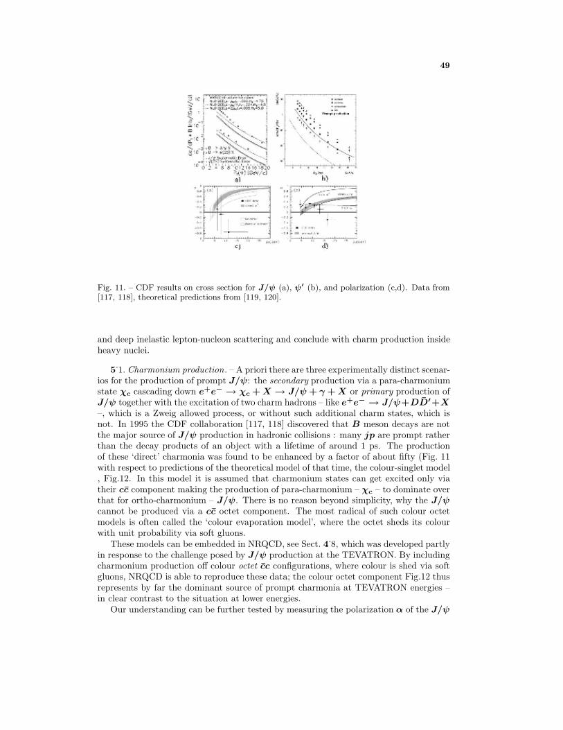
49

Fig. 11. – CDF results on cross section for J/ψ (a), ψ′ (b), and polarization (c,d). Data from[117, 118], theoretical predictions from [119, 120].

and deep inelastic lepton-nucleon scattering and conclude with charm production insideheavy nuclei.

5.1. Charmonium production. – A priori there are three experimentally distinct scenar-ios for the production of prompt J/ψ: the secondary production via a para-charmoniumstate χc cascading down e+e− → χc +X → J/ψ+ γ +X or primary production ofJ/ψ together with the excitation of two charm hadrons – like e+e− → J/ψ+DD′+X–, which is a Zweig allowed process, or without such additional charm states, which isnot. In 1995 the CDF collaboration [117, 118] discovered that B meson decays are notthe major source of J/ψ production in hadronic collisions : many jp are prompt ratherthan the decay products of an object with a lifetime of around 1 ps. The productionof these ‘direct’ charmonia was found to be enhanced by a factor of about fifty (Fig. 11with respect to predictions of the theoretical model of that time, the colour-singlet model, Fig.12. In this model it is assumed that charmonium states can get excited only viatheir cc component making the production of para-charmonium – χc – to dominate overthat for ortho-charmonium – J/ψ. There is no reason beyond simplicity, why the J/ψcannot be produced via a cc octet component. The most radical of such colour octetmodels is often called the ‘colour evaporation model’, where the octet sheds its colourwith unit probability via soft gluons.

These models can be embedded in NRQCD, see Sect. 4.8, which was developed partlyin response to the challenge posed by J/ψ production at the TEVATRON. By includingcharmonium production off colour octet cc configurations, where colour is shed via softgluons, NRQCD is able to reproduce these data; the colour octet component Fig.12 thusrepresents by far the dominant source of prompt charmonia at TEVATRON energies –in clear contrast to the situation at lower energies.

Our understanding can be further tested by measuring the polarization α of the J/ψ

50

Fig. 12. – Colour-singlet and colour-octet diagrams for hadroproduction (left) and e+e− produc-tion (right) of charmonium; photons and gluons are denoted by wave and curly lines, respectively.

and ψ′ defined as (dΓ/d cos θ) ∝ 1 + α cos2 θ in the angular distribution of decayleptons pairs from charmonium; α = 1[−1] corresponds to pure transverse [longitu-dinal] polarization. Both charmonia states are predicted [119, 120] to be increasinglytransversely polarized with growing p⊥ since one expects the transverse polarization ofalmost ‘on-shell’ gluons to be transferred to the cc bound state produced from them.However this effect is certainly not apparent in the data, see Fig.refFIG:CDFJPSI c), d)[121]. Again, this might not be a fatal flaw in NRQCD; it might just mean that contribu-tions of higher order in αS and in v are still sizeable for charmonia and affect polarizationmore than cross sections, which are more robust against higher order contributions.

Real photoproduction experiments provide also results on hidden charm states, whosediffractive production proceeds via VMD coupling of the beam photon to JPC = 1−−

mesons such as J/ψ. Such studies are generally limited to dimuon final states, sincedielectron decay modes are hindered by the presence of electron-positron pairs copiouslyproduced by Bethe-Heitler mechanisms. Very recently, the first observation of ψ(3770)was preliminarily reported by FOCUS [123].

Experiments E760 and E835 at the Fermilab antiproton source have performed pre-cision measurements of all charmonium states, also measuring the χc1 for the first time.Charmonium states are produced by the collisions of antiprotons on a hydrogen jet target,thus providing interaction whose geometry is effectively the one typical of fixed targetexperiments. Experiment E835 charmonium results are discussed in Sect.6.

5.2. Charm at LEP (mainly). – With no hadron being present in the initial state,e+e− annihilation represents the simplest scenario. At the same time charm was thefirst quantum number high enough in mass that one can invoke perturbative QCD todescribe e+e− → hadrons below as well as above its threshold; i.e., the ratio R hadreached a constant value below threshold and a higher one above it.

One of the most intriguing aspects theoretically has been discussed in Sect.4.11,namely how quark-hadron duality and the approach to it is realized in nature. Theconclusion is that starting at about 1 GeV above threshold perturbative QCD can beemployed for predicting the total cross section for e+e− → hadrons. The experimentalsituation just above charm threshold had been somewhat unsettled with some data sets

51

showing an unusually large cross section. Measurements [124] done by the BES collabora-tion in Beijing have clarified the situation; the value of R does not seem to be excessivelylarge. Future studies from CLEO-c should settle it completely. The transition regionaround 4 GeV will presumably remain beyond theoretical control, since so many thresh-olds for exclusive final states open up: e+e− → DD, D∗D +DD∗, D∗D∗, D+

s D−s ,

..., ΛcΛc etc.. One can attempt to describe this highly complex landscape through mod-els involving a coupled-channel approach [125, 126]; yet the predictions based on suchmodels are not reliable, since they are quite unstable under variations of the model pa-rameters. Nevertheless important measurements can be performed there: in particularthe absolute branching ratios for the different charm hadrons can be measured in a modelindependent way as explained in Part II of this review.

BELLE has shown highly surprising data on double cc production: it finds the J/ψto be accompanied more often than not by an additional cc pair [127]:

σ(e+e− → J/ψcc)

σ(e+e− → J/ψX)= 0.59+0.15

−0.13 ± 0.12(73)

There is no good idea from theory (yet) how such a large ratio could be accommodated.Measurements by HRS, MARK II and TASSO at the PETRA and PEP storage rings

at DESY and SLAC, respectively, had provided the first reliable information on thefragmentation functions of charm and beauty quarks described in Sect. 5.6. Yet they havebeen superseded by ARGUS and CLEO measurements with their much higher statisticsand by LEP and SLD data, the latter for beauty as well as charm quarks; see [128, 129]for concise reviews. CLEO finds a deviation from a Peterson et. al.-type fragmentationfunction for D+

s ,D∗+s [130]. It is actually more difficult to measure the charm than the

beauty fragmentation fragmentation at LEP, since in the case of charm one has to relyon exclusively reconstructed charm hadrons to obtain sufficient purity of the sample,which reduces considerably the statistics [131]. Furthermore an interpretation of thedata is less straightforward, among other reasons due to the secondary production ofcharm via gluon splitting g → cc. Nevertheless there exists a strong twofold motivationfor determining the charm fragmentation function as accurately as possible: (i) it is animportant ingredient in predicting charm production cross sections and distributions tobe measured at the TEVATRON; (ii) comparing it to the beauty fragmentation functionwill shed further light on the nonperturbative dynamics driving it.

The level of production can be computed (with mc = 1.5 ± 0.3 GeV), and whencompared to recent data [129] it is found a couple of standard deviations below.

LEP experiments provide information on charm production through studies of γγ →cc, where the initial state is realized by initial state radiation off both beams . Recentresults are discussed in Ref. [112]. D∗± production has been measured by LEP experi-ments at

√s = 183−209 GeV and found in agreement with NLO QCD predictions. L3

also measured σ(γγ → ccX) as a function of the γγ invariant mass finding reasonableagreement with NLO QCD for mc = 1.2 GeV; for mc = 1.5 GeV one predicts a 50%lower cross section.

Another observable that can be computed in NLO QCD is the aforementioned gluonsplitting probability gcc of cc for (e+e− → qqg, g → QQ). An OPAL result yieldsgcc = (3.20 ± 0.21 ± 0.38) × 10−2 [132], which is higher than theoretical estimatesas well as the L3 measurement [133] gcc = (2.45 ± 0.29 ± 0.53) × 10−2. LikewiseALEPH and DELPHI find higher than predicted values for the corresponding quantitygbb.

52

An area of great importance to the validation of the electroweak sector of the StandardModel is the determination of the forward-backward asymmetries for charm and beautyjets AccFB, A

bbFB, and the ratios of charm and beauty quark partial widths Rb, Rc Rc =

Γ(Z0 → cc)/Γ(Z0 → hadrons), see [134, 135] for an extensive review. The charmFB asymmetries had been measured before the LEP era [136], [137], [138], but only thehuge data sets gathered at LEP allowed meaningful searches for manifestations of NewPhysics. The situation has changed considerably over the years, as it can be realizedbrowsing the LEP Electroweak Working group pages [139]. Measurements of Rb, Rc in1995 [140] differed from SM predictions by +3.7σ,−2.56σ, while they appeared totallyconsistent in 2002 [141] +1.01σ,−0.15σ. On the other hand, AccFB, A

bbFB that in 1995

were completely consistent with the SM within their relatively large errors, in 2002represent a pull of −0.84σ,−2.62σ respectively, with AbbFB being the second largestcontribution of pulls in the fit to the SM parameters, after the intriguing NuTeV resulton sin2 θW [142].

5.3. Photoproduction. – The real photon has two components, namely a hadronic one ala vector meson dominance , and one coupling directly to quarks via their electric charge.Due to the small weight of the former, photon beams provide a cleaner environment thanhadron beams since mostly there is no hadronic jet from beam fragmentation. One stillhas to contend with a large background of light hadrons. Yet the charm-to-total cross-section ratio of about 1/100 is considerably higher than the 1/1000 for hadroproduction.Also the theoretical treatment of photoproduction is easier than of hadroproduction sinceonly one hadron participates in the collision.

The recent success in gathering sizeable samples of events with both charm and anti-charm hadrons allows novel probes of perturbative QCD and has already lead to newinsights on QCD dynamics.

Scattering electrons off protons at small values of Q2 provides a fluid transitions toreal photoproduction experiments with Q2 = 0. In real photoproduction high-energy,high-intensity beams impinge on nuclear targets and can produce charm states. Thetree-level production mechanism proceeds via the fusion[143] of beam photon off a gluonemitted by the nucleus (Fig. 10).

The charm cross-section is sensitive to the charm quark mass, and it has been thor-oughly measured from threshold up to HERA energies, and compared to QCD predictions[116]. A value of 1.5 GeV for the pole charm quark mass is favoured by the data withlarge errors due to the choice of other theory parameters.

Real photoproduction is studied via the very large data samples collected by fixedtarget experiments [111]. The reconstruction of both D and D in the same event allowsone to study DD correlations that can be predicted in principle by QCD. Importantvariables are ∆φ, the angle between the particle and the antiparticle in the plane trans-verse to the beam, and the transverse P 2

T momentum squared of the pair. At leadingorder, with cc quarks produced back to back, one expects ∆φ = π and PT = 0. Recentresults from FOCUS [144] show that data disagree with predictions even when takinginto account NLO contributions. There is also a small but highly significant excess ofdata at ∆φ = 0 suggesting that a small fraction of DD pairs are produced collinearlyrather than back-to-back. These studies are a valuable tool to tune charm productioncomputational algorithms, such as PYTHIA [145].

Particle-antiparticle asymmetry studies have been carried out in the past by photopro-duction experiments NA14/2[146], E691 [147] and E687[148]. E691 and E687 measurea significant asymmetry for D+, D0 and D∗+, and one compatible with zero within

53

large experimental errors for D+s ,Λ

+c . The asymmetry measured is ten times the one

predicted by perturbative QCD. Mechanisms based on heavy-quark recombination havebeen proposed [149]. High statistics results from FOCUS are expected soon.

Finally, FOCUS [150] showed recently a null result on the production of double charmbaryons reported by hyperon beam experiment SELEX [151] [152]. The issue is addressedin Sects.6 and 6.3.5.

5.4. Fixed target hadroproduction. – Experiments have been performed with a host ofextracted meson as well as baryon beams and also internal beams on gas targets.

The leading particle effect is the most interesting phenomenological feature in charmproduction studies with extracted beams. This is the enhancement of the production ofparticles compared to the production of antiparticles, and it is due to the presence ofquarks present both in the produced particle, and in the target nucleon or in the beamparticle. The enhancement is represented (usually in a differential fashion in xF andP 2T ) via the asymmetry variable

A ≡ Nparticle −Nantiparticle/R

Nparticle +Nantiparticle/R(74)

where R ≡ ε/ε is the ratio of acceptances for particles and antiparticles.As a matter of principle perturbative QCD can yield only a very small asymmetry in

charm production; in contrast asymmetries as large as 50% have often been reported inthe data. In the following we shall limit ourselves to outline the most striking features ofcharm production at extracted beams, referring the interested reader to recent reviews[153], [154], [111].

Tree-level hadroproduction proceeds via diagrams shown in Fig. 10(a,b). At fixed tar-get, the availability of several kinds of beam allows one to study the leading particle effect.Recent results come from E791 (π− beam) and SELEX (π−, proton and Σ− beams) .Asymmetry data for Λ+

c produced by π− beams in E791 and SELEX do agree, whilethe asymmetry for proton and Σ− beams in SELEX is much more pronounced, a clearmanifestation of leading particle effect, since baryon beams will produce preferentiallyΛ+c baryons, not antibaryons.SELEX recently reported observation of four different C = 2 baryons [151] [152]. If

confirmed, it would have profound implications for our understanding of charm produc-tion. We will discuss this issue in Sect.6.3.5.

5.5. Hadroproduction at colliders . – The study of charm physics at hadronic colliderswas pioneered at the CERN ISR (see Sect.3.2). Experiments done there showed evidencefor much larger charm cross sections than expected, in particular in the forward regionof up to 1.4 mb. It was finally understood that such high values were due to efficiencyand acceptance corrections used to get cross sections out of low-acceptance mass-peakobservations [155],[156].

The most lasting legacy is maybe the concept of intrinsic charm suggested a long tomeago by Brodsky and collaborators [157] to account for the larger charm production inthe forward or projectile fragmentation region. It says that protons (and other hadrons)have a cc component that unlike in the conventional picture is not concentrated in the‘sea’ at very small values of fractional momenta x: |p〉 ∝ |uud〉 + |uudcc〉 + ‘sea′.This has been referred to as a higher Fock state in the proton wave function. Therehas been and still is an ongoing debate over the validity of this intriguing picture and

54

the danger of double-counting. It seems now that in the framework of the heavy quarkexpansions one can assign the concept of intrinsic charm an unambiguous meaning [158].

Little new work theoretically as well as experimentally has been done on charm pro-duction at hadron colliders until recently. This lull seems to be coming to an end now.Most of our community was quite surprised when in 1991 CDF [159] demonstrated theability of studying beauty quark physics in a pT regime totally unsuited for the main-stream W physics the detector was conceived for. CDF’s capabilities have been furtherboosted by the implementation of a detached vertex trigger described in Sect.3.2, whichprovides online selection of events based on reconstructed decay vertices by the microstripdetector. The vertex trigger might allow reconstruction of charm correlations.

So far we have results on D∗ production [67, 112]. In 2000 CDF published theonly available measurements of open charm production cross sections in pp collisions at√s = 1.8TeV for the processD∗+ → D0π+ → (K−µ+X)π+ for in the rapidity and

transverse momentum intervals |η(D∗+)| < 1.0, pT (D∗+ > 10GeV ). The integratedcross section found σ = 347 ± 65 ± 58nb exceeds calculations based on both NLO andFONLL.

5.6. Deep inelastic lepton-nucleon scattering. – As already mentioned in Sect.2, thefirst experimental signal for charm production outside cosmic rays came from dimuonevents in deep inelastic neutrino nucleon scattering [14]

νµN → µ−Hc +X → µ−µ+ + X(75)

Also some early charm spectroscopy had been done in neutrino induced events. Today’smain lessons from charm production by neutrinos are the following:

• It provides important information on |V (cs)| & |V (cd)|, as described in Part II.

• It allows extraction of the structure functions for d and s quarks and antiquarksfrom open charm and for the gluons from J/ψ production.

• In νX → l−Λ+c X one can measure the form factor of Λc baryons in the space-like

region [160].

• Since Λc is expected to be produced with a high degree of longitudinal polarization,one could search for a T odd correlationCT odd ≡ 〈~σΛc ·(~pΛ×~pl)〉 in semileptonicΛc decays νN → Λ+

c X → (l+νΛ)Λc +X

• To determine the fundamental electroweak parameters at lower energies in differentkinematical domains one has to understand – or at least model reliably – charmproduction, since it varies with energy and is different in charged vs. neutral currentreactions. A very simple ansatz is often used here, namely the ‘slow rescaling’model, where one replaces the usual scaling variable x by

x → ξ = x

(1 +

”mc”2

Q2

)(1 − x2MN

Q2

)(76)

It should be noted that ”mc” here is merely a quark model parameter. Measuringits value with high accuracy from ν data does not mean we know the charm quarkmass till we can derive Eq.(76) from QCD.

55

Charm production occurs in high energy neutrino interactions at the few percent leveland to lowest order is described by the diagram in Fig.10 f), with strong dependence tothe strange quark sea, since charm production off d quarks is Cabibbo-suppressed. Thissensitivity is further enhanced in the case of antineutrino scattering, where only sea dand s quarks contribute with the latter dominating.

A wealth of results keeps coming from charm neutrino experiments using emulsion andelectronic techniques, namely NOMAD and CHORUS at CERN and NuTeV at FNAL[113]:

• Emulsion experiments have been able to measure the inclusive charm productioncross-section σ(νµN → cµ−X)/σ(νµN → µ−X) which is of order five percent,while electronic experiments measured the inclusive D production rate σ(νµN →D0µ−X)/σ(νµN → µ−X) about two percent. A recent analysis [161] combinesboth electronic and emulsion experiments results.

• Insights are gained on the hadronization of charm quark described through fragmen-tation functions, see Sect.4.2. It should be noted that the fragmentation processis expected to be universal, i.e., independent of the hard scattering process understudy; i.e., charm quarks emerging from, say, e+e− collisions dress into charmedhadrons in the same fashion as those produced in lepton-nucleon scattering. Cross-section data for neutrino production are parameterized via the usual Peterson formD(z) ∝ [z(1 − z−1 − εP /(1 − z))]−1, and the customary kinematical variablesp2T , fh (the mean multiplicity of charmed hadron h) and z (the fraction of the

quark longitudinal momentum carried by the charmed hadron). The fragmenta-tion function D(z) is peaked at z = 0.8 which means that the hadronizationprocess is hard, and relatively energetic. Neutrino experiments measure the εPparameter and compare it to e+e− data, generally finding good agreement for D∗

production.

Charm production in neutrino physics is thus an alive field, where great interest existsfor the huge improvements which are expected at a Neutrino Factory [160], [162].

A new realm of analyzing heavy flavour production – of charm and beauty, open andhidden – has opened up in high energy

√s = 300−318GeV electron-proton collisions

studied at HERA by the H1, Zeus and HERA-C collaborations. Production of charmhadrons and charmonia can occur off gluons, cc pairs in the sea at small values of x andoff an intrinsic charm component at medium and large values of x [157]. The stage isthus more complex than in e+e− annihilation – yet that should be viewed as a virtue,since data allow us access to these parton distribution functions.

Not only the proton target adds complexity to the phenomenology, but also the elec-tron projectile, which effectively acts either as in deep inelastic lepton-nucleon scattering, (Fig.10 c), or in photoproduction (Fig.10 d), depending on the Q2 region considered.In the photoproduction regime (Q2 ∼ 0), then, the photon can produce charm via adirect point-like coupling to partons in the proton (Fig.10 d), or it can effectively actas a hadron a la vector meson dominance, Fig.10 e). In the latter case, any intrinsiccharm components in the photon or proton particles may give origin to charm excitationprocesses, such as cg → cg. The variable xobsγ is normally used to discriminate directfrom resolved photon processes.

The experimental panorama is discussed in recent reviews [112, 163, 114]. Photopro-duction cross-sections for D∗ and Ds generally exceed the next to leading order (NLO)

56

QCD predictions, as well as the fixed order plus next to leading logarithm (FONLL) cal-culations [164]. The photoproduction cross section is also measured as a function of xobsγ .This allows to show that a relevant contribution from charm excitation processes needsto be taken into account by theory. In DIS electroproduction regime (Q2 > 1 GeV2)D∗ cross sections are compared to predictions and found in fair agreement, althoughsomehow undershooting data. The NRQCD prediction for J/ψ production yields a ris-ing cross section for z ≡ EJ/ψ/Eγ → 1, i.e. the kinematic boundary – in conflict withobservation.

Another observable predicted by NRQCD predictions is the ratio of diffractive pho-toproduction rates of J/ψ vs. ψ(2S). New data from H1 are found to be consistentwith NRQCD predictions [165].

Resolved photon processes are expected to dominate the low-z inelastic region, whiledirect photon processes should dominate the region up to about z ∼ 0.9, with diffractivephotoproduction taking over at z ∼ 1. Recent H1 and ZEUS results are reviewedand compared [114] to colour singlet (CS) and colour singlet + colour octet (CS+CO)predictions. As explained in Sect.4.8, the CO component enters naturally in NRQCDmodel, and is fitted to the large J/ψ cross section measured by CDF in 1995. HERAdata are consistent with CS+CO contributions, although data do not rise as a functionof z as rapidly as CS+CO predictions do. On the other hand, in electroproductionregime Q2 > 2GeV 2, the inelastic J/ψ cross section measured by H1 clearly favoursCS predictions.

Yet it would be premature to condemn NRQCD for this apparent discrepancy; for inits present level of sophistication it is not applicable in this kinematical domain. Futurerefinements of NRQCD should enable us to extend its applicability there.

5.7. Hadroproduction inside heavy nuclei . – The fabric of QCD is such that it cancreate an extremely rich dynamical landscape. To explore it fully one has to go beyondobserving reactions involving single hadrons. When heavy nuclei collide with hadronsor other heavy nuclei the interactions between individual hadrons take place against thebackground of nuclear matter; this can lead to highly intriguing phenomena, of whichwe sketch two examples, namely the lowering of the D meson mass and colour screeninginduced by the quark-gluon plasma .

Most of the mass of pions and kaons, which are Goldstone bosons, is due to howapproximate chiral symmetry is realized in QCD. Spontaneous chiral symmetry breakingleads to the emergence of non-vanishing quark and gluon condensates. Chiral invarianceis partially restored in the medium of nuclear matter. It is expected that the massespions and kaons exhibit inside nuclei get changed relative to their vacuum values, andthat there is even a split between the masses of charge conjugate pairs with the nuclearmedium providing an effective CPT breaking; it has been predicted that the masses ofπ+ and π− [K+ and K−] get shifted by about 25 [100] MeV. Experimental evidencefor such effects has been inferred from the observation of pionic atoms and the study ofthe onset of K+ and K− production in heavy-ion collisions.

The situation is qualitatively different – and richer – in the charm sector since therethe mass is due mostly to the c quark mass, and different scales enter the dynamics for theinteractions with the nuclear medium. For the J/ψ and ηc only a small mass reductionof around 5 - 10 MeV is predicted, since charmonium masses are affected by mostlygluon condensates. D mesons on the other hand offer the unique opportunity to studythe restoration of chiral invariance in a system with a single light valence quark [34]. Alowering of both D± masses is predicted with a relative shift of ∼ 50 MeV in M(D+)

57

vs. M(D−). One of the items in the GSI HESR proposal is to study these effects indetail in pAu collisions. Very intriguing effects are expected in the charm thresholdregion: at normal nuclear density the DD thresholds falls below the ψ′ resonance; attwice nuclear density this threshold moves below even the χc2!

The fact that hidden charm states are significantly less extended than open charmstates has been invoked as a signature for the quark-gluon plasma, where the correlationbetween colour sources and sinks is broken up over small distances. If in heavy ioncollision a phase transition to the quark-gluon plasma is achieved, one expects a reductionin J/ψ production. The data are intriguing in this respect, yet not conclusive.

Charmonium production is investigated in relativistic heavy ion collisions[166], wherethe NA50 experiment [167, 168] using 1996 data (158 GeV per nucleon Pb beams onPb target) provided circumstantial evidence for charmonium suppression, which may beexplained by the onset of a quark-gluon plasma regime. They measure J/ψ productionrelative to Drell-Yan pair production. After accounting for conventional nuclear absorp-tion, their data show evidence for a suddenly lower production, due to the attractingforce between the cc quarks being screened by gluons, and fewer cc pairs hadronizinginto J/ψ.

To conclude this section, we discuss a fascinating as much as hypothetical possibilityuniquely provided by the study of charm particles in close contact to nuclear media, i.e.,the formation of supernuclei. In complete analogy to what has been studied in greatdetail for several decades in Λ-hypernuclei [169], a charm quark produced at rest, orbrought to rest, could interact with the nuclear matter, replace a light quark, and form aΛC baryon inside the nucleus. The ΛC would then decay. This is an appealing processbecause the ΛC does not need to obey the Pauli exclusion principle, and can occupynuclear levels forbidden to the nucleons. The lifetime is also expected to differ from thatfor free ΛC , and it would be possible to study both mesonic and nonmesonic decays.The only attempts carried out so fare have been in emulsions [170]. Supernuclei studiesare foreseen at GSI with the PANDA experiment (see Part II).

6. – Spectroscopy and Lifetimes

The minimal information to describe a particle are its mass and its spin (13). Underthe term ‘mass’ we can include also the width as the imaginary part of the mass. Thewidth or lifetime of a particle actually characterizes its underlying dynamics in a way thatthe (real) mass cannot, namely whether they are strong (even if reduced), electromagneticor weak, and in the latter case whether they are CKM suppressed or not. Beyond thesegeneral remarks the situation is different for hidden and open charm hadrons.

Hidden charm states cc are characterized by a Compton wave length ∼ 2/mc ∼1/3 fm, i.e. their extension is somewhat smaller than for light-flavour hadrons. Theycan decay electromagnetically and even strongly, the latter however with a very reducedwidth since it is order α3

S(mc) (for J/ψ). Powerful algorithms have been and are beingdeveloped to obtain very accurate predictions on charmonium spectroscopy from latticeQCD thus turning their experimental study into precision tests of QCD proper .

(13)This can be expressed for the mathematically minded reader by saying that elementaryparticles are defined by irreducible representations of the Poincare group; for those are labeledby the eigenvalues of two Casimir operators, which happen to be the mass and spin (or helicityfor massless particles).

58

As already explained in Sect.4.5 HQS tells us that for open heavy flavour hadrons thetwo S wave configurations PQ and VQ become mass degenerate for mQ → ∞, whiletheir mass exceeds mQ by the scale ∼ ΛNPD (14) as do the P wave configuration. I.e.:

mc + ΛNPD ∼ MD ' MD∗ , MD∗∗ ∼ MD + ΛNPD(77)

The degree to which the hyperfine splitting MD∗ −MD is small compared to ΛNPD isone measure for whether charm is a heavy flavour. It is, though not by a large factor:

MD∗ −MD ∼ 140 MeV < MD∗∗ − 〈MD〉 ∼ 480 MeV(78)

with 〈MD〉 = 14MD + 3

4MD∗ denoting the spin averaged meson mass. Also the simple

scaling law of Eq.(12) is well satisfied:

MB −MD ' 3.41 GeV vs. MΛb −MΛc ' 3.34 GeV(79)

There are further reasons to study the mass spectroscopy of charm resonances:

• For a better understanding of the transition B → lνD∗ that figures prominentlyin determinations of V (cb) – and ofB → lνXc in general – one needs informationon the mass and width of D∗∗ and other higher resonances.

• More specifically, the SV sum rules [87] relate the basic HQP to the production ofcertain charm states in semileptonic B meson decays. E.g. [81]:

1

2= −2

∑n

∣∣∣τ (n)1/2

∣∣∣2 +∑m

∣∣∣τ (m)3/2

∣∣∣2

Λ(µ) = 2

(∑n

εn

∣∣∣τ (n)1/2

∣∣∣2 + 2∑m

εm

∣∣∣τ (m)3/2

∣∣∣2)

µ2π(µ)3

=∑n

ε2n

∣∣∣τ (n)1/2

∣∣∣2 + 2∑m

ε2m

∣∣∣τ (m)3/2

∣∣∣2µ2G(µ)

3= −2

∑n

ε2n

∣∣∣τ (n)1/2

∣∣∣2 + 2∑m

ε2m

∣∣∣τ (m)3/2

∣∣∣2 ;(80)

here εk denotes the excitation energy of the final state Dk beyond the groundstates D and D∗ (εk = MDk −MD) while τ (n)

1/2 and τ (m)3/2 denote the transition

amplitudes for producing a state, where the light degrees of freedom carry angularmomentum jq = 1/2 or 3/2, respectively [171]. Obviously, the masses of thesecharm resonances matter, as does their interpretation in terms of the quantumnumbers 1/2 or 3/2.

• The mass splittings of baryonic charm resonances provide important cross checksfor the evaluation of expectation values of four-quark operators that are highlyrelevant for predicting charm baryon lifetimes as discussed below.

(14)It is usually denoted by Λ.

59

Beyond classification there are other reasons for measuring total widths as preciselyas possible. One needs them as an engineering input to translate branching ratios intopartial widths. This is needed, for example, to infer the value of CKM parameters fromsemileptonic decays. On the phenomenological level a precise analysis of the D0 lifetimeis a prerequisite for studying D0 − D0 oscillations. Finally on the theoretical side thelifetime ratios for the different charm hadrons provide the best, since most inclusiveobservables to probe hadrodynamics at the charm scale.

From the raison d’etre for charm quarks, namely to suppress strangeness changingneutral currents to the observed levels, one infers mc ≤ 2 GeV. The lifetime of charmquarks can be estimated by relating it to the muon lifetime and the number of colours

and lepton flavours τc ∼ τµ ·(mµ

mc

)5

· 1NC+2

∼ (few 10−13s) ·(

1.5 GeVmc

)5

with anobviously high sensitivity to the value of mc.

These very simple estimates have turned out to be remarkably on target. Yet beforewe describe it, a few comments might be in order on the charm quark mass.

6.1. On the charm quark mass. – Within a given quark model a quark mass hasa clear meaning as a fixed parameter; however it depends on the specifics of the dy-namical treatment adopted there, and therefore differs from model to model. Yet evenmore importantly the connection between such quark model parameters and fundamentalquantities appearing in, say, the Lagrangian of the SM is rather tenuous. For exampleone can model single and double charm production in deep inelastic ν-nucleon scatteringby charged and neutral currents with a parton model ansatz, where mc plays of coursea central role. Fitting data can yield a highly constrained value for mc. Yet such a ‘pre-cise’ value cannot be taken at face value to describe charm hadroproduction, let alonecharmonium physics or charm decays. For that purpose one needs a proper field theo-retical definition of the charm quark mass, which takes into account that the dynamicalenvironments for these reactions differ in their perturbative as well as nonperturbativeaspects. The resulting quantity has to be a ‘running’, i.e. scale dependent mass, whereone has to specify its normalization scale; these issues have been discussed in Sect.4.6.3.

The two areas where quark masses have been discussed with considerable care arecharmonium spectroscopy and the weak decays of heavy flavour hadrons.

1. The first analysis was based on charmonium sum rules that approximate nonper-turbative dynamics through including quark and gluon condensates in the OPE[172]. One finds for the MS mass

mc(mc) = 1.25 ± 0.10 GeV(81)

More recent analyses find fully consistent values:

mc(mc) =

1.19 ± 0.11 GeV Ref .[173]1.30 ± 0.03 GeV Ref .[174](82)

Lattice studies yield in the quenched approximation [175]

mc(mc) = 1.301 ± 0.034 ± 0.13quench GeV .(83)

60

2. The expansion for mb −mc given in Eq.(21) yields

mb −mc = 3.50 GeV + 40 MeV(µ2π − 0.5 GeV2

0.1 GeV2

)± 20 MeV(84)

Using the value for the b quark mass that has been extracted from e+e− → bbnear threshold by several groups [176]

mkinb (1 GeV) = 4.57 ± 0.08 GeV = mb(mb) = 4.21 ± 0.08 GeV(85)

which is in nice agreement with what one infers from a moment analysis of semilep-tonic B decays [177], and Eq.(84) one arrives at

mc(mc) = 1.13 ± 0.1 GeV .(86)

This value is completely consistent with what one obtains directly from the afore-mentioned moment analysis, namely

mc(mc) = 1.14 ± 0.1 GeV(87)

despite the caveats stated in Sect.4.6.3 about the reliability of this expansion.

3. As will become clear from our discussion below, one cannot infer (yet) a reliablevalue for mc from the charm lifetimes.

To summarize: a quite consistent picture has emerged, which supports treating charmas a heavy flavour.

6.2. Spectroscopy in the hidden charm sector . – Charm entered reality in a mostdramatic fashion through the discovery of hidden charm mesons and their striking prop-erties, and our knowledge about them increased at breathtaking speed for some time dueto very favourable experimental features.

Most of the spectroscopy results have come from e+e− storage rings, where JPC =1−− states can be formed directly to lowest order. The three prominent statesJ/ψ(3100),ψ′(3700) and ψ′′(3770) have been well established for a long time as the 3S1, 23S1

and 3D1 states, respectively, with the last one being broad since above DD productionthreshold. The nonvector states such 3PJ (also referred to as χcJ) and 1S0 can bereached by E1 and M1 transitions from them and thus be observed in two–step pro-cesses like e+e− → ψ′ → (cc)χcJ + γ, see Fig. 13. This area of research pioneered bySPEAR and DORIS has experienced a welcome renaissance due to the operation of theBeijing Spectrometer (BES); in 2002 the BES collaboration has completed a four-monthrun which yielded 14 million ψ(2S), to be added to the 4 million events previouslycollected.

A qualitatively new access to charmonium dynamics has been provided by low energypp annihilation, since all JPC quantum numbers then become accessible, in particularalso 1P1 and 1D2 and 3D2 states. The idea (pioneered by R704 at the ISR and carriedforward by E760, E835 at FNAL) is to study the formation of charmonia states in theannihilation of antiprotons on a jet hydrogen target. E835 showed [121, 122] preliminarymeasurements of masses, widths and branching ratios of the three χcJ states with anunprecedented level of precision.

61

Finally a third actor has appeared: the B factories CLEO, BABAR and BELLEhave such large statistics that one can study charmonia in B → [cc]X. This has beendemonstrated quite dramatically by BELLE finding 5 σ and 3.5 σ signals for ηc(1S) andηc(2S), respectively [178, 127]. The ηc(2S) can boast of quite a saga [179]. Previoussimultaneous observations of ηc and ηc(2S) date back to conflicting measurements inthe 1980’s (DASP, Serpukhov, MARK II and Crystal Ball). While the ηc has becomewell established, the ηc(2S) was not confirmed by either DELPHI or E835 in extensivesearches (30 pb−1 in the range 3666 to 3575 MeV). 2000 E835 searched with higherstatistics for the ηc(2S), with negative results. The ηc(2S) was instead spotted in 2002by BELLE at 3622 ± 12 MeV in B decays, and 3654 ± 6 MeV in the recoil spectrumof J/ψcc events. Similarly frustrating is the search for the singlet P-state called hc.Claimed by R704 at the ISR in 1986 and seen by E760 in 1993, the hc has not, as yet,been confirmed by E760’s successor E835 in its 2001 data set.

One expects [180] four charmonium states below DD threshold (and thus narrow),whose existence has not been established, namely η′

c(21S0), hc(11P1), ηc2(11D2) and

ψ2(13D2); they can be identified in B decays.The potential model ansatz pioneered by the Cornell group [181] was successful in

describing the charmonium spectroscopy of Fig. 13). The factorization of nonpertur-bative and perturbative effects into a wave function and αS corrections, respectively,as mentioned in Sect.4.1.1 can be seen from the theoretical expression for the hadronicwidth of the J/ψ: Γ(J/ψ → hadrons) = 80(π2−9)

81παs(MJ/ψ)3(1 + 4.9αs

π)|Ψ(0)|2.

The ratio of this to the leptonic width can be used to extract a value of αs: Rµµ =J/ψ→hadronsJ/ψ→µ+µ− = 5(π2−9)

81π

αs(MJ/ψ)3

αem(1+10.3αs

π). The experimental value Rµµ ≈ 14.9

leads to a reasonable result: αs(MJ/ψ) ≈ 0.2. Relativistic effects of order v2/c2 canalso be included. Yet this method of extracting αs is not as theoretically sound as oth-ers. The first order radiative correction is as large as the lowest order correction callinginto question the validity of the perturbative expansion. Furthermore, the expressionsfor the various widths ultimately depend on the expression that is chosen to describethe quark-antiquark potential, which is based upon phenomenological aspects of QCDrather than rigorously derived from it. By taking ratios, in which the dependence on thewavefunctions vanish, this source of uncertainty can be reduced. It still remains unclearhow valid the factorization assumption is for the charmonium system in which mc isonly moderately larger than typical hadronic scales.

Radiative transitions between charmomium states can similarly be described. Theradius of the bound state is typically much smaller than the wavelength of the emittedradiation so a multipole expansion is expected to converge quite rapidly. Electric dipole(E1) transitions are responsible for ∆S = 0,∆L = 1 processes. The rate for transitionsbetween S- and P- wave states is:

Γγ(S ↔ P ) =4

9

(2Jf + 1

2Ji + 1

)Q2α|Eif |2E3

γ .(88)

Here Jf [i] denotes the total angular momentum of the final[initial] state, Q = 2/3 is thecharge of the charmed quark, Eγ is the photon energy and Eif is the matrix element ofthe transition dipole operator: Eif =

∫∞0r2Ψi(r) rΨf (r). Since this matrix element

is more sensitive to the exact shape of the wavefunction unlike |Ψ(0)|2 that appearedpreviously, considerable differences emerge among theoretical predictions. Even so, thereis reasonable agreement with experiment [126]. Magnetic dipole (M1) transitions are

62

(2S)ψ

γ∗

ηc(2S)

ηc(1S)

hadrons

hadrons hadrons

hadrons

radiative

hadronshadrons

χc2(1P)

χc0(1P)

(1S)ψJ/

=JPC 0−+ 1−− 0++ 1++ 1+− 2++

χc1(1P)

π0

γ

γ

γ

γγ

γ

γγ∗ hc(1P)

ππη,π0

hadrons

Fig. 13. – Chart of charmonium states [128].

responsible for ∆S = 1,∆L = 0 processes and are suppressed by Eγ/mc with respectto the E1 transitions. The transition rate between spin 0 and 1 S- wave states is givenby the following expression:

Γγ(3S1 ↔1 S0) =16

3(2Jf + 1)

(Q2

2mc

)α|Mif |2E3

γ .(89)

Here the magnetic dipole moment is the expectation value of the zeroth order sphericalBessel function: |Mif | =

∫∞0 r2Ψi(r) j0(1

2Eγr)Ψf (r). Since these matrix elements

depend quite sensitively on details of the wave functions, it is not surprising that theagreement between theory and experiment for M1 transitions is rather poor.

The lattice community is able now to treat charmonium physics with three flavoursof dynamical quarks; from the spin-averaged 1P −1S and 2S−1S splittings one infersfor the strong coupling αMS

S (MZ) = 0.119 ± 0.004 [182].Hadronic transitions like ψ′ → ψππ are also treated using a multipole expansion

to describe the gluonic radiation. An added complication is the hadronization of theemitted gluonic radiation. By introducing a chiral Lagrangian to describe the effectivelow energy behaviour of the hadronic state, a semi-quantitative analysis can be carriedout for these transitions.

The transition Jψ → γX driven by Jψ → γgg provides a gluonic origin forthe final state X. Accordingly states with a particular affinity to gluons should figureprominently in X. Narrow states would show up as mass peaks in the γ recoil spectrum;no prominent signal has been found yet. One can search for them also in exclusive finalstates, as discussed in Part II of this review.

6.3. Spectroscopy in the C 6= 0 sector . – Adding charm as the fourth quark leads toa very rich spectroscopy. There are six C = 1 pseudoscalar states (plus one cc statealready discussed) in addition to the familiar SU(3) meson nonet, namelyD±, D±

s andD0/D0; likewise for the vector mesons with D∗±, D∗±

s and D∗0/D∗0. For baryonseven more facets emerge, as described later.

These states can be fitted into SU(4) multiplets. Yet SU(4) breaking driven by

63

sD0D

sD

–D

0K–π π

+K

–K

(a)

sD

DD

sD

−ρ +ρ

K

(b)*0

K*−

*+K*0

D 0*D*−

*−

*+

−

*+

−cdcu−

cs−

us−ds−

su− sd− ud

−

uc−sc−

dc−

0ρ ωφψJ/

uc−sc−

dc−

−cdcu−

cs−

+

D+

+

K 0

us−ds−

su− sd−

du−

du−

0D

ηη′ηc

π 0

ud−

K 0*

Ξ +c

Σ ++c

Ξ 0

n pΞ c

0

Ω+cc

Ξ ++ccΞ +

cc

Σ 0c

Σ −Σ +Λ,Σ 0

Σ +cΛ+

c,

Ω 0c

(b)

Σ ++c

Ξ +c

Λ+c

0cΞ

(c) Λ

Ω++ccc

Ξ ++ccΞ +

cc

Ω+cc

Σ ++c

Ξ +cΞ 0

c

Ω −Ξ 0

Σ +

∆+∆0∆−

Σ −

Ξ −

∆++

(a)

Σ 0

cΣ +Σ 0

c

Ω 0c

Ξ +c

Σ ++c

uscdsc dsc usc

uucudc

ssc

ddcΣ +

cΛ+c

udc

Ξ c0 Ξ'c

0 Ξ'c+

Ω 0c

Σ 0c

Fig. 14. – Chart of ground state charmed meson and baryon multiplets [128].

mc > ΛNPD ms is much larger than SU(3) breaking (15). Heavy quark symmetryprovides a much more useful classification scheme. As explained in Sect.(4.5) for heavyflavour hadrons HQ the spin of Q – SQ – decouples from the light quark degrees offreedom, and jq ≡ sq + L and SQ become separately conserved quantum numbers. Ameson [baryon] can then be characterised by the spin of the light antiquark [diquark]and the orbital angular momentum.

While the masses of the groundstates D/D∗ and Ds/D∗s have been known with

1 MeV precision for a decade now, the experimental information available on other statesis still unsatisfactory. In this section we shall discuss open problems and very recentsurprises.

6.3.1. D∗ width. Measuring Γ(D∗+) represents an experimental challenge: suchwidths are predicted in the range of tens or hundreds keV, and must be experimen-tally deconvoluted to the experimental resolution of detectors. CLEO has presented thefirst measurement [183, 184] based on the sequence D∗+ → π+D0, D0 → K−π+

from a 9 fb−1 sample of e+e− data collected with the CLEO II.V detector. Γ(D∗+)is controlled by the strong coupling constant, since the electromagnetic contributionD∗+ → γD+ produces a very small branching ratio, and can thus be neglected.

Based on an involved analysis of 11,000 reconstructedD∗ decays CLEO finds Γ(D∗+) =96 ± 4 ± 22 keV. Hence they infer for the D∗Dπ coupling: gD∗Dπ = 10 ± 3.5.Light-cone sum rules have been employed to obtain the prediction [185] gD∗Dπ =17.9 ± 0.3 ± 1.9, where the value 13.5 is viewed as a rather firm upper bound [186].

The B factories with their large charm samples should be able to check CLEO’sresults, once detector simulation will reach the level of accuracy necessary to tame thesevere systematic uncertainty.

6.3.2. Charm mesons - L = 1 excited states. For each of the cu, cd and cssystems four P-wave and two n = 2 radial excitations have been studied. There arefour L = 1 states, namely two with jq = 1/2 and total spin J = 0, 1 and two withjq = 3/2 and J = 1, 2. These four states are named respectively D∗

0 , D1(jq = 1/2),

(15)Another way to put it is to say that charm mesons – unlike pions and kaons – cannot beviewed as Goldstone bosons.

64

Fig. 15. – Masses and transitions predicted for the excited D meson states.

D1(jq = 3/2) and D∗2 (Fig.15). Parity and angular momentum conservation force the

(jq = 1/2) states to decay to the ground states via S-wave transitions (broad width),while (jq = 3/2) states decay via D-wave (narrow width). To be more specific, for the1/2 one predicts widths of ∼ 100 MeV and for the 3/2 of about ∼ 10 MeV with theexception of the Ds1(jq = 3/2)(2536) which is kinematically forced to a ∼ 1 MeVwidth.

All six L = 1, j = 3/2 narrow states are well established, with precisions on massesat the 1 MeV level and on widths at the few MeV level. This is due to the fact thatexcited D states are abundantly produced both at FT experiments, in e+e− continuumproduction, in B decays and at the Z0 [134]. Common analysis techniques are the selec-tion of a clean sample of D meson candidates typically via a candidate-driven algorithm(see Sect.6.4.1), a cut on the Dπ mass to reject D∗ compatible combinations, and thepairing of the D candidate with one (two) soft pion (pions) in the primary vertex to formthe D∗∗ candidate. A selection on the helicity angle is effective in selecting L=1 statesfrom background, as well as in selecting different states in the same final channel.

At e+e− one also invokes the mass constraint of the fixed center of mass energy andkinematical helicity cuts which exploit the constraint of the parent B mass. Dalitz plotand partial wave analyses have also been presented [187].

A review of the data from different experiments can be found in [189]. A commonfeature is a prominent peak in the 2460 MeV region, escorted by satellite peaks at oneπ0 mass below, due to feeddown from decays where the π0 escapes detection, such asthe decay chain D∗+

2 → D0π+ with the D0 wrongly assigned to D∗0 → D0π0 decay.Generally speaking, narrow L=1 signals at FT have higher statistics but sit on a

more prominent background, due to the larger combinatorics coming from larger primarymultiplicities. On the other hand photoproduction signals with their lower primarymultiplicity have less combinatorics than hadroproduction.

The status of the broad L=1 states is much less clear, and the assignments of thequantum numbers are largely based on theory expectations for their masses and widths.In 1998 CLEO [190] showed evidence for the D1(jq = 1/2) broad state. The authorsof Ref.[191] propose an alternative interpretation of this state as the axial chiral partner.Such an alternative interpretation is actually supported by the SV and spin sum rulesdescribing semileptonic B decays, see Eq.(80): they strongly suggest that the D∗∗ statesaround 2.4 − 2.6GeV have to come mainly from a 3/2 state – or they do not represent

65

Table III. – Winter ’02/’03 status of (L=1, n=1) and (L=0, n=2) cq and cs mesons (MeV).Statistical and systematical errors added in quadrature. Experimental results not included inPDG [128] are from BELLE [187], CLEO [190], DELPHI [193], FOCUS [194] [195]. Theorypredictions from [196].

jq 1/2 1/2 3/2 3/2 1/2 1/2JP 0+ 1+ 1+ 2+ 0− 1−

L, n 1, 1 1, 1 1, 1 1, 1 0, 2 0, 2

D∗0 D1 D1(2420) D∗

2(2460) D′ D∗′

Decay Mode Dπ D∗π D∗π Dπ,D∗π D∗ππ

Mass (MeV)PDG 0 2422 ± 2 2459 ± 2PDG ± 2427 ± 5 2459 ± 4 2637 ± 7FOCUS 0 ∼ 2420 2463 ±2FOCUS ± ∼ 2420 2468 ±2BELLE 0 2290 ± 30 2400 ± 36 2424 ± 2 2461 ± 4DELPHI ± 2470 ± 58CLEO 0 2461 ± 51Theory 2400 2490 2440 2500 2580 2640

Width (MeV)PDG 0 19 ± 4 23 ± 5PDG ± 28 ± 8 25 ± 7 < 15FOCUS 0 ∼ 185 30 ± 4FOCUS ± ∼ 185 29 ± 4BELLE 0 305 ± 40 380 ± 140 27 ± 4 46 ± 5DELPHI ± 160 ± 77CLEO 0 290 ± 100Theory >170 >250 20-40 20-40 40-200

D∗s0 Ds1 Ds1(2536) D∗

sJ (2573) D′s D∗′

s

Decay Mode D∗K DK

Mass (MeV)PDG ± 2535.3 ± 0.6 2572.4 ± 1.5FOCUS ± 2535.1 ± 0.3 2567.3 ± 1.4Theory 2480 2570 2530 2590 2670 2730

Width (MeV)PDG ±. <2.3 90 % cl 15 ± 5FOCUS ± 1.6 ± 1.0 28 ± 5Theory < 1 10 − 20

a P wave configuration [192].Tab.III gives a summary of our knowledge of excitedD mesons as it appeared in early

2003. At that time it seemed all one needed was to fill in a few gaps.A major confirmation for HQS would be the definite observation of the missing (L =

1, jq = 1/2, JP = 0+) D∗0 and (L = 1, jq = 1/2, JP = 1+) D1 broad states. More

recently, FOCUS[194] and BELLE[187] showed new preliminary results and evidencefor D∗

0. Errors on both masses and widths are still very large and we expect bettermeasurements from the B-factories due to their larger data sets.

The overall information on L=1 cs states is unsatisfactory anyway. The Ds1(jq =

66

3/2) has been seen in D∗K0 final state, and not in D+K0 or in D0K+. The Ds12

(called DsJ(2573) by PDG) has been seen in D0K+ and recently in D+K0[195].Furthermore no candidate for the Ds(1/2) doublet had been seen yet. Since theirmasses were firmly expected to be about 80 MeV larger than for the correspondingnonstrange states, they would have enough phase space for the decays into D(∗)K finalstates leading to large widths.

An open question remains the first evidence[197] seen by DELPHI of a charm radialexcitation D∗′+ in the D∗+π−π+ final state (called D ∗ (2640)± by PDG); it has notbeen confirmed by any experiment (OPAL[198], CLEO[199], ZEUS[200], and questionedby theory predictions [201].

6.3.3. Charm mesons - New L = 1 Ds states. Analyses presented by BABAR [202]and CLEO [203] in the spring of 2003 are challenging the whole picture.

1. BABAR reported finding a narrow resonance D∗sJ(2317) with D∗

sJ(2317) →D+s π

0 in 90fb−1 of data. With the observed width consistent with the experi-mental resolution, the intrinsic width has to be below 10 MeV. This discovery hasbeen confirmed by CLEO.

2. CLEO with 13fb−1 has observed another similarly narrow state at a mass 2.46GeV, for which BABAR had found evidence before: D∗

sJ(2463) → D∗+s π0.

It seems natural to interpret D∗sJ(2317) and D∗

sJ(2463) as 0+ and 1+ states, respec-tively. The decay distributions are consistent with such assignments, yet do not estab-lish them. They together with the mass values would explain the narrow widths: forD∗s1+(2463) → DK is forbidden by parity,D∗

s0+(2317) → DK and D∗s1+(2463) →

DK∗ by kinematics and D∗s0+(2317) → D+

s π0 and D∗

s1+(2463) → D∗+s π0 are

isospin violating transition and thus suppressed. Also D∗s0+(2317) → D+

s γ is forbid-den.

There are three puzzling aspects to these states:

• Why have no other decay modes been seen ? In particular CLEO places a lowupper bound

BR(D∗s0+(2317) → D∗+

s γ) < 0.078 90% C.L.(90)

Why is it not more prominent, when D∗s0+(2317) → Dsπ

0 is isospin violating ?

• Why are their masses so much below predictions ? One should note that a deficitof ∼ 160 and ∼ 100 MeV is quite significant on the scale of M(D∗

sJ) −M(D).Why is the mass splitting to the previously found narrow states Ds1(2536) andDsJ(2573) so much larger than anticipated ?

• A related mystery is the following: where are the corresponding non-strange charmresonances ? They should be lighter, not heavier thanD∗

s0+(2317) andD∗s1+(2463).

Potential model results have been re-analyzed, lattice QCD is being consulted [204] andmore exotic scenarios like a DK molecule below threshold [205] and other four-quarkinterpretations have been put forward. The latter are hard pressed to explain the narrowwidth in the first place, since the transition would not have to be isospin violating; yet inaddition CDF sees no evidence for D∗

sJ → Dsπ± [206], although the preliminary CDF

67

2.10 2.20 2.30 2.40 2.50 2.60M(Dsπ

0) (GeV/c2)

0

40

80

Eve

nts/

5MeV

/c2

0.10 0.20 0.30 0.40 0.50 0.60M(Dsπ

0)-M(Ds) (GeV/c2)

0

40

80

Eve

nts/

5MeV

/c2

Data

qq Monte Carlo

(a)

(b)

(a)

(b)

M(Dsγπ0) - M(Dsγ) (GeV/c2)

Eve

nts

/ 5 M

eV/c

2

0

10

20

0

10

20

0.1 0.2 0.3 0.4 0.5 0.6

Fig. 16. – New D∗s0+(2317) and D∗

s1+(2463) states observed by BABAR (a,b) [202] and CLEO(c,d) [203].

data of well known L=1 states (such as the D∗2) reported so far show rather modest

signal-to-noise ratios.Maybe the most intriguing explanation, since it would represent a new paradigm for

the implementation of chiral invariance, is the suggestion made in Ref.[207] to combineheavy quark symmetry and chiral invariance in a novel way: the latter is realized throughparity doublets pairing (Ds,D∗

s) with (D∗s0+,D

∗s1+). Chiral dynamics induces a mass

splitting ∆M between the heavy quark doublets: invoking a Goldberger-Treiman rela-tion [208] the authors of Ref.[207] estimate

∆M = M(D∗s0+) −M(Ds) ' M(D∗

s1+) −M(D∗s) ∼ mN/3(91)

in agreement with the experimental findings. They also find that the radiative width isreduced: BR(D∗

s0+(2317) → D∗+s γ) ∼ 0.08, i.e. right about CLEO’s upper limit.

The same chiral symmetry and ∆M apply to B mesons and double charm baryons[ccq].

Last – but certainly not least – the same chiral splitting should arise for nonstrangecharm mesons leading to

M(D±(0+) ' 2217 MeV , M(D±(1+) ' 2358 MeV(92)M(D0(0+) ' 2212 MeV , M(D0(1+) ' 2355 MeV(93)

Of course, these predictions could be modified significantly by order ΛNPD/mc cor-rections. These states can decay strongly into Dπ and D∗π and thus would be broad.This makes it difficult to distinguish the decays of these resonances from phase spacedistributions of Dπ and D∗π. It is very important to search for them; finding themwould neccessitate a new interpretation for the previously listedD∗

0 andD1. B factoriesanalysing the final states of B decays have an advantage in such analyses.

These remarks indicate that a fundamental re-evaluation of strange as well as non-strange charm hadrons might be in store. This would have an important impact not onlyon charm spectroscopy, but also on the aforementioned sum rules describing semileptonicB decays, Eq.(80), and on the latter’s interpretation.

6.3.4. C = 1 baryons. In the framework of SU(4) (Fig.14) we expect nine groundstate cqq JP = 1/2+ baryons (all of them detected after the 1999 CLEO II.V observa-tion of Ξ′

c) and six cqq JP = 3/2+ baryons (with only the Ω∗0c remaining undetected,

68

after the observation of Σ∗+c by CLEO II.V in 2002 [209]); for a concise and for a more

detailed review see [128] and [219], respectively. The Ω∗0c is expected to decay via the

experimentally challenging channel Ω∗0c → γΩ0

c ) (16).Only a few of the orbitally excited P-wave (L = 1) baryons have been observed. The

first doublet Λc1(2593) (1/2−) and Λ∗c1(2625) (3/2−) was observed several years

ago by CLEO II.V, ARGUS, and E687. In 1999 CLEO II.V presented evidence[211] forthe charmed-strange baryon analogous to Λ∗

c1(2625), called Ξ∗c1(2815), in its decay to

Ξcππ via an intermediate Ξ∗c state. The presence of an intermediate Ξ∗

c instead of Ξ′c

supports an 3/2− assignment, while HQS explicitly forbids a direct transition to the Ξcπground state due to angular momentum and parity conservation. More recently, CLEOhas reported on the observation of both a broad and a narrow state in the Λ+

c π+π−

channel, identified as the Σc1 and the Λc0 1/2− [212].Mass splittings within isospin multiplets are caused by QCD corrections due to

md > mu and by electromagnetic effects. Interest in this subject has attracted new in-terest recently: while for all well-measured isodoublets one increases the baryon mass byreplacing a u–quark with a d–quark, the opposite happens in the case of the poorly mea-sured Σ++

c (cuu) − Σ0c(cdd) isosplit [213, 214]. Also, as discussed below, the SELEX

candidates for the two isodoublet C = 2 baryons Ξcc show larger than expected masssplitting. FOCUS’ new number M(Σ++

c ) − M(Σ0c) = −0.03 ± 0.28 ± 0.11 MeV

[215] indicates a trend towards a smaller splitting, although still statistically consistentwith both E791 one’s of 0.38±0.40±0.15 MeV as well as PDG02’s 0.35±0.18 MeV.

There is another use of baryonic spectroscopy in a somewhat unexpected quarter: asexplained in Sect. 4.6.2 and discussed more specifically below, the weak decay widths ofcharm baryons can be expressed through the expectation values of local operators. Thenumerically leading contributions are due to four-quark operators. At present we cancompute those only with the help of wave functions obtained in quark models. Yet thosewave functions allow us also to calculate baryon mass splittings. One can then relatethe needed baryonic expectation values to static observables like M(Σc) − M(Λc) orM(Σ∗

c) −M(Σc) [216]. Uraltsev, Phys. Lett. B 376 (1996) 303Finally, measurements of the Σc,Σ++

c natural widths were presented by CLEO[217]and FOCUS[218]. They both agree on a few MeV width, but the level of precision is notenough yet to discriminate among theoretical models.

6.3.5. C ≥ 2 baryons. Combining the large charm production rates in hadroniccollisions with state-of-the-art microvertex detectors that allow to trigger on charm decaysopens the window to a more exotic class of hadrons, namely baryons containing two (oreven three) charm quarks. There is an SU(3) triplet of such states: Ξ++

cc = [ccu],Ξ+cc = [ccd] and Ω+

cc = [ccs] (plus the superheavy Ωccc = [ccc]).Like for C = 1 baryons, one can employ quark models of various stripes to predict

their masses. However there are some qualitative differences: as stated before, in the Λcand Ξc bound states a light spin-zero diquark surrounds the heavy c quark, whose spinis decoupled to leading order in 1/mc due to QCD’s HQS. In Ξcc and Ωcc on the otherhand the light degrees of freedom carry spin 1/2 implying degeneracy among severalground states to leading order in 1/mc. It has been suggested to model C = 2 baryons

(16)We adopt for excited baryon states the nomenclature in [210]. Thus, members of 3/2multiplets are given a (∗), the subscript is the orbital light diquark momentum L, and (′)indicates symmetric quark wavefunctions cq1q2 with respect to interchange of light quarks,opposed to antisymmetric wavefunctions c[q1q2].

69

as a heavy-light system consisting of a cc-diquark and a light quark. Accordingly therewill be two kinds of mass spectra, namely due to excitations of the light quark and of thecc ‘core’. Based on such an ansatz the following predictions on the masses were mademore than ten years ago [220]:

M(Ξcc) ' 3.61 GeV, M(Ωcc) ' 3.70 GeV, M(Ωccc) ' 4.80 GeV,(94)

These numbers still reflect today’s theoretical expectations [221, 222]. Ref.[221] listsvarious models; their predictions are in the range 3.48 - 3.74 GeV for M(Ξcc) and 3.59- 3.89 GeV for M(Ωcc).

In 2002, the SELEX Collaboration claimed the observation [151] of the Ξ+cc (ccd)

through its decay mode to Λ+c K

−π+. In this experiment charmed baryons are pro-duced by a 600 GeV charged hyperon beam (Tab.I). Charged tracks are detected andreconstructed by a silicon vertex detector, coupled to a forward magnetic spectrome-ter. After analyses cuts, a sample of 1630 fully reconstructed Λc → pK−π+ eventsis selected. Double charm baryon candidates are searched for in events which assign aΛc to a K−π+ secondary vertex. SELEX found a 15.9 events signal over an expectedbackground of 6.1 ± 0.5 events, that they translate to a 6.3σ significance, at a massof 3519 ± 1 MeV, and a width of 3 MeV compatible to the experimental resolution.SELEX has also shown [152] preliminary results on an excess of 9 events (over an ex-pected background of 1), at 3460 MeV, which they translate to a 7.9σ significance inthe Λ+

c K−π+π+ final state. This was interpreted as evidence for the isodoublet part-

ner, the Ξ++cc . Alternate statistical approaches have been proposed [223] which treat

differently the background fluctuations, and provide a signal significance for the SE-LEX candidates of about 3-4 σ. The very serious trouble with this interpretation isthe apparent ∼ 60 MeV mass splitting between the isospin partners Ξ+

cc and Ξ++cc : it

causes a major headache for theorists, in particular when one keeps in mind that theproper yardstick for comparing this mass splitting to is not the total mass, but the muchsmaller binding energy of a few hundred MeV. Furthermore as discussed above there isno evidence for such an exotic effect in single charm baryons.

In May 2003 a very intriguing new twist has been added to the story: based onfurther studies, in particular of the angular distributions of the decay products, SELEX[224] now concludes that there are actually four C = 2 baryons, namely two J =1/2+ states with L = 0, namely Ξ+

cc(3443) and Ξ++cc (3460) decaying isotropically

into Λ+c K

−π+ and Λ+c K

−π+π+, respectively, and a heavier pair Ξ+cc(3520) and

Ξ++cc (3541) presumably with J = 1/2− and L = 1 decaying nonisotropically into the

same final states. The problem with the isospin mass splittings mentioned above hasbeen alleviated now, since the two isodoublets have mass splittings of 17 and 21 MeV,although this is still anomalously large. The heavier doublet could be understood as anexcitation of the cc core; preliminary estimates yield for this excitation energy a rangeof about 70 to 200 MeV and for the isospin mass splitting about 6 MeV [225].

The SELEX evidence has not been confirmed by the photoproduction experimentFOCUS[226]. In FOCUS, following analysis techniques similar to SELEX, a sampleof 19,444 Λc → pK−π+ events is selected, with neither Ξ+

cc nor Ξ++cc candidates.

FOCUS concludes (Tab. IV) that this implies a production difference between doublecharm baryons and Λc baryons of > 42 for the Ξ+

cc, and > 111 for the Ξ++cc .

SELEX’ interpretation of its data creates very considerable headaches for theory. Theobserved isospin splitting is larger than expected, yet the main problem concerns the re-ported lifetimes. None of the four states exhibit a finite lifetime, and the apparent upper

70

Table IV. – Comparison of SELEX and FOCUS results on double-charm baryons (from [226]).Limits are at the 90% cl.

Ξ+cc → Λ+

c K−π+ Ξ++

cc → Λ+c K

−π+π+

FOCUS SELEX FOCUS SELEXΞcc Candidate events <2.21 % 15.8 <2.21 % 8Reconstructed Λc 19 500 1 650 19 500 1 650Ξcc/Λc Relative Efficiency 5% 10% 13% 5%Relative Yield Ξcc/Λc <0.23 % 9.6 % <0.09% 9.7%Relative Production Ξcc/Λc SELEX/FOCUS >42 SELEX/FOCUS >111

bound is about 33 fs. One should note that the upper doublet can decay electromag-netically through M2 transitions, for which one can estimate a lifetime of about 1 fs[225]. Therefore if they indeed represent C = 2 baryons, their weak lifetimes have to beindeed on the femtosecond level. The poses a very serious challenge to theory, as will bediscussed in Sect. 6.5.

Not unlike BELLE’s observation of J/ψcc events [227] SELEX’ findings point tounexpectedly large cccc production. Yet they present another puzzle as well, namelywhy two charm quarks each produced in a hard collision presumably incoherently endup in the same C = 2 baryon. One would expect that much more often than not theyhadronize separately leading to sizeable DD and DD production.

6.3.6. Production of charm resonances. A very naive estimate for the relative produc-tion of different charm states is based on ‘spin counting’, i.e. assigning equal probabilityto the production of each spin component of a given charm hadron. Consider the sim-plest case of vector (V ) vs. pseudoscalar (P ) production like D∗ vs. D. Spin countingsuggests a ratio r = V/(V + P ) = 3/4. There is no justification (beyond its sim-plicity) for such an ansatz and it fails already for continuum Ds∗ vs. Ds production ine+e− annihilation, where CLEO finds [228] r = 0.44 ± 0.04 which is less than evenequal production for D∗

s and Ds. In semileptonic B decays on the other hand one findsΓ(B → lνD∗) ∼ 2Γ(B → lνD).

With the increase in data sets, and the simultaneous refinement in the level of sophis-tication in understanding the sources of systematics, measurements of relative productionyields of L=1 states in B decays have become available.

There is a double motivation for understanding charm production in B decays – inparticular semileptonic B decays – that goes well beyond testing hadronization modelsper se.

• The CKM parameter |V (cb)| is best extracted from B → lνXc, B → lνD∗ andB → lνD. To fully understand detection efficiencies, feed-downs etc. one has toknow the quantum numbers of the charm final states produced.

• The sum rules stated in Eq.(80) relate the basic heavy quark parameters to mo-ments of the production rates for jq = 1/2 and jq = 3/2 charm resonances.Those heavy quark parameters form an essential input for the theoretical treat-ment of semileptonic B decays, beauty lifetimes etc. and also provide a valuablequantitative test ground for lattice QCD.

71

It has been known for a long time that charm production in B decays is characterizedby the dominance of broad over narrow states. Since the former are usually identifiedwith jq = 1/2 and the latter with jq = 3/2 this is again in clear contrast to spincounting.

The BELLE paper [187] discusses the issue. Their measurements show that narrowresonances compose 33±4% of the B → (Dπ)π decays, and 66±7% of B → (D∗π)πdecays. This trend is consistent with the excess of broad states component in semileptonicB decays B → D∗∗`ν at LEP [188]

One should keep in mind though that these assignments 1/2 vs. 3/2 are typicallyinferred from theory rather than the data. It was already mentioned that the sum rulesof Eq.(80) cast serious doubts on some of these assignments.

Only a few theoretical papers have addressed the issue of relative production ratesof L=1 states, from B decays. Neubert[229] predicts the ratio J=2 / J=1(j=3/2) R =B(B → D∗0

2 π−)/B(B → D0

1(j = 3/2)π−) ∼ 0.35 while BELLE measures [187]R=0.89+−0.14; both numbers actually contradict spin counting.

The Orsay group[230] has developed a model for describing charm production inexclusive semileptonic B decays. The model predicts dominance of narrow states in Bsemileptonic decays. It can claim reasonable reliability, since it implements the SV andspin sum rules referred to in Eq.(80).

As for L=1 D mesons not produced from B decays, there are no theoretical predictions.The only experimental evidences here for broad states come from FOCUS [194], wherethe D∗

0 is observed relative production yields with respect to the D∗2 of about 3:1.

6.4. Weak lifetimes and semileptonic branching ratios of C = 1 hadrons . – The decayrate of a charm quark provides only an order of magnitude estimate for the lifetimes of theweakly decaying charm hadrons; their individual lifetimes could differ quite substantially.

To illustrate this point, let us look at strange quarks and hadrons. Very naively onewould expect for a strange quark of mass 150 MeV a (Cabibbo suppressed) lifetime ofroughly 10−6 s. Not surprisingly, such a guestimate is considerably off the mark. Fur-thermore strange hadrons exhibit huge lifetime differences which are fed by two sources:

τ(KL)

τ(KS)∼ 600 ,

τ(K+)

τ(KS)∼ O(100) ∼ τ(K+)

τ(Λ)(95)

The first ratio is understood as the combination of (approximate) CP invariance in kaondecays, which forbids KL to decay into two pions, with the accidental fact that the KL

mass is barely above the three-pion threshold. Such an effect cannot induce a significantlifetime difference among charm hadrons. For the second and third ratio in Eq.(95) aname has been coined – the ∆I = 1/2 rule – yet no conclusive dynamical explanationgiven. Since all weakly decaying strange baryons benefit from ∆I = 1/2 transitions,no large lifetime differences among them arise. The impact of the ∆I = 1/2 rule isseen directly in the ratio of the two major modes of Λ decays: Γ(Λ → nπ0)/Γ(Λ →pπ−) ' 1/2.

Even before charm lifetimes were measured, it had been anticipated that as a ‘first’for hadronic flavours the lifetime of a few ·10−13 sec predicted for c quarks providesa meaningful benchmark for the lifetimes of weakly decaying charm hadrons and thelifetime ratios for the latter would differ relatively little from unity, certainly much lessthan for strange hadrons.

72

The semileptonic branching ratios provide a complementary perspective onto non-perturbative hadrodynamics. The semileptonic widths of charm mesons are basicallyuniversal meaning that the ratios of their semileptonic branching ratios coincide withthe ratios of their lifetimes. Yet the semileptonic widths of charm baryons are expectedto vary substantially meaning that the ratios of their semileptonic branching ratios yieldinformation over and above what one can learn from the ratios of their lifetimes.

6.4.1. Brief History, and Current Status of Lifetime Measurements. Unstable particlesdecay following an exponential law P (t) = exp(−t/τ), whose constant slope τ isdefined as the mean decay time in the particle’s rest frame, i.e., the lifetime. Charmlifetimes were expected in the range of 10−12 − 10−13. In the lab frame, a particle getstime-dilated by a factor γ = E/m, and a measurement of the decay length ` providesdetermination of the proper decay time ` = γβct for each decay event. The slope ofthe exponential distribution of decay lengths ` is the particle’s lifetime. The decay is aprobabilistic effect following an exponential distribution, therefore one needs adequatestatistics, and precise measurement of decay length and particle momentum.

For an experiment at fixed target, where charm particles are produced with a typicalaverage momentum of 50 − 60GeV, the expected charm lifetime translates to decaylengths of order one centimeter. At symmetrical colliders, where the charm particleis produced at rest in the lab frame, the decay length is very short, and one cannotdetermine it by directly observing the separation between primary (production) vertexand secondary (decay) vertex, but needs to use an impact parameter technique. For adetailed review on experimental techniques see [231].

The space resolution at fixed target in the transverse plan is often of a few microns,which translates on a resolution in reconstructing the decay vertex of order 10 microns inx,y and 300 microns in z. When coupled to a forward magnetic spectrometer with goodmomentum resolution, the resolution on the decay time is of order 30-50 fs. At colliderexperiments the decay length is very small, due to the lack of substancial Lorentz boost.High-resolution drift chambers are used for vertex detection, or, recently, microstriparrays deployed in 4π geometry. The primary vertex is detected as the beam spot inthe interaction region. Tracks of secondaries are reconstructed as helices in (ρ, ϕ) plane.Distribution of proper decay times is not an exponential as in the fixed target case,but a gaussian with an right-hand exponential tail, due to the relatively poorer spaceresolution. Proper time resolution, thanks to better momentum resolution, of state ofthe art e+e− collider experiments is now comparable to fixed target experiments.

The output signals from the vertex detector are used in track- and vertex-findingalgorithms. The principal approach for vertex finding is the candidate-driven algorithm.It consists of determining a set of tracks which have been particle-identified and thatare compatible with a charm decay topology. Tracks are requested to be compatible ascoming from a common decay vertex. The reconstructed charm particle momentum isthen projected to the primary vertex, thus determining the primary-secondary separation` and error σ`. At e+e− (Ref.[232],[233]), candidate tracks are fit to a common vertex,the reconstructed momentum is projected to the interaction region to obtain the decaylength.

A selection cut which requires the presence of a parent D∗ for D0 lifetimes (D∗-tagging) may be used, albeit at the cost of a reduction in statistics. To cope with thereduced reconstruction efficiency at small decay lengths, one uses the reduced proper timet′ ≡ (`−Nσ`)/βγc where N is the primary-secondary detachment cut applied. Usingt′ instead of t corresponds to starting the clock for each event at a fixed detachment

73

Table V. – Summary of world averages from [128], new results, and updated world averages.Statistical and systematical errors are summed in quadrature.

Experiment Lifetime (fs) Events Channels Techn.

D+ New Average 1045 ± 8FOCUS [234] 1039.4 ± 8 110k K2π γNBELLE(prel) 1037 ± 13 8k K2π e+e−

PDG02 1051 ± 13

D0 New Average 410.6 ± 1.3FOCUS [234] 409.6 ± 1.5 210k Kπ,K3π γNBELLE(not incl) 416.2 ± 1.1(st) 214k Kπ e+e−

PDG02 411.7 ± 2.7

D+s New Average 494 ± 5

FOCUS [235] prel 506 ± 8(st) 6k φπ γNBELLE [237] prel 485 ± 9 6k φπ e+e−

PDG02 490 ± 9

Λ+c PDG02 200 ± 6

Ξ+c PDG02 442 ± 26

Ξ0c New Average 108 ± 15

FOCUS 118 ± 14 110 ± 17 Ξ−π+,Ω−K+ γN

PDG02 98+23−15

Ω0c New Average 76 ± 11

FOCUS [238] 79 ± 15 64 ± 14 Ω−π+,Ξ−K− 2π+ γNPDG02 64 ± 20

significance, and thus the distribution of t′ recovers exponential behaviour.Main sources of systematics at fixed-target are absorption of both secondary tracks

and charm in target, knowledge of D momentum, backgrounds, and montecarlo eventsample size. For e+e− colliders, the determination of the decay vertex, beam spot,knowledge of D momentum, time-mass correlations, large t outlier events, decay lengthbias, backgrounds, and montecarlo event sample size.

New results are shown in Tab.V, with updated world averages with respect to PDG02.Lifetimes ratios significant for comparison to theoretical predictions are listed in Tab.VI.While the accuracy on the lifetimes of long-lived mesons is now at the level of the percent,essentially systematics-dominated, the measurement of very short-lived charm states,such as the ΩC , still poses relevant challenges. In this case the superior decay timesresolution of fixed-target experiments (of order 30 fs), although comparable to the lifetimeitself, does allow lifetime determination at the level of 15%.

6.4.2. Early phenomenology. All charm hadrons share one contribution, namely theweak decay of the charm quark, which to leading order is not modified by its hadronicenvironment, see Fig. ( 17). It is often called the spectator process, since the otherpartons present in the hadron (antiquarks, quarks and gluons) remain passive bystanders

74

(17). This reaction contributes to all charm hadrons equally scaling like

ΓSpect ∝ G2Fm

5c(96)

Originally it had been expected that this term dominates the lifetime already for charmhadrons implying a small difference between τ(D0) and τ(D+). It caused quite a stir inthe community when the lifetime measurements showed the D+ to be longer lived thanthe D0 by a considerable factor [239, 240]. It enhanced the drama that the first data‘overshot the target’, i.e. yielded τ(D+)/τ(D0) ∼ 5 before ‘retreating’ to a ratio of∼ 2.5. This surprise caused considerable activities on the theory side to accommodatethe data and make new predictions for the other lifetime ratios.

Two mechanisms were quickly put forward as to induce τ(D+)/τ(D0) > 1:

1. On the Cabibbo-favoured levelW -exchange can contribute toD0, as shown in Fig.( 18 a), but not to D+ transitions. The latter are affected only on the Cabibbosuppressed level by W exchange in the s-channel, Fig. ( 18 b).

2. In the reaction D+ = [cd] → sdud one has two identical quark flavours in thefinal state, see Fig. ( 19). Interference effects thus have to be included, whichturn out to be destructive for nontrivial reasons. This effect is referred to as PauliInterference (PI) .

The first mechanism had been known all along, yet its contributions had been discardedfor a reason. For it suffers from two suppression factors, namely helicity suppressionand wavefunction suppression: (i) With spin-one couplings conserving chirality, a pseu-doscalar meson cannot decay into a massless fermion-antifermion pair. Thus the am-plitude for W -exchange is proportional to the mass of the heaviest quark in the finalstate: T (D0 → sd) ∝ ms/MD . This is a repetition of the well known tale whyΓ(π+ → µ+ν) Γ(π+ → e+ν) holds. (ii) Due to the almost zero range of the weakforce the c and u quark wavefunctions have to overlap to exchange a W boson. Thedecay constant fD provides a measure for this overlap: fD ' √

12|ψcu(0)|/√MD.Accordingly T (D0 → sd) ∝ fD/MD.

Putting everything together one obtains ΓWX(D0) ∝ G2F |fD|2m2

smD rather thanΓSpect ∝ G2

Fm5c . Since ms, fD mc such a W-exchange contribution is very small.

Yet after the data revealed a large lifetime ratio, various mechanisms were suggested thatmight vitiate helicity suppression and overcome wavefunction suppression. Most of themwere quite ad-hoc. One that appeared natural was to invoke gluon emission from theinitial light (anti)quark line leading to

ΓWX(D0 → sdg) ∝ αS

π

(fD

〈Eu〉)2

G2Fm

5c(97)

with 〈Eu〉 denoting the average energy of u inside the D0. Despite the double penaltyone pays here – it is a term ∼ O(αS/π) controlled by three-body rather than two-bodyphase space – such a contribution could be sizeable for 〈Eu〉 ∼ fD.

(17)The reader should be warned that some authors use the term ‘spectator contribution’ forprocesses where the ‘spectators’ become active.

75

Fig. 17. – The diagram describing the weak decay of the charm quark. This spectator processcontributes to the width of all charmed hadrons.

A distinction had been made between W exchange and weak annihilation with theweak boson being exchanged in the t and s channels, respectively. Yet since QCDrenormalization mixes those two diagrams, it is more meaningful to lump both of themtogether under the term weak annihilation (WA) as far as meson decays are concerned;Wexchange in baryon decays, which is not helicity suppressed, is denoted by W scattering(WS) .

While the occurrence of PI in exclusive D+ decays had been noted, its relevance forinclusive D+ rates had been discarded for various reasons. Yet in a seminal paper [239]it was put forward as the source of the observed lifetime ratio.

Both mechanisms can raise τ(D+)/τ(D0) considerably above unity, yet in differentways and with different consequences: (i) While PI reduces Γ(D+) without touchingΓ(D0), WA was introduced to enhance Γ(D0) while hardly affecting Γ(D+). As aconsequence, since ΓSL(D+) ' ΓSL(D0) due to isospin invariance, PI will enhanceBRSL(D+) while not changing BRSL(D0), whereas WA will decrease BRSL(D0) whilehardly affecting BRSL(D+). (ii) For PI one expects τ(D0) ∼ τ(Ds), whereas WAshould induce a difference in τ(Ds) vs. τ(D0) roughly similar to τ(D+) vs. τ(D0).(iii) One would expect to see different footprints of what is driving the lifetime differencesin the weight of different exclusive modes like Ds → π′s vs. Ds → φ + π′s vs.Ds → KK + π′s.

Weak baryon decays provide a rich laboratory for these effects: WS is not helicitysuppressed in baryon decays, and one can count on it making significant contributionshere. Furthermore PI can be constructive as well as destructive, and its weight is morestable under QCD radiative corrections than is the case for meson decays. On fairlygeneral grounds a hierarchy is predicted [241]:

τ(Ωc) < τ(Ξ0c) < τ(Λc) < τ(Ξ+

c )(98)

It should be noted that all these analyses invoked – usually implicitly – the assumptionthat a valence quark description provides a good approximation for computing suchtransition rates. For if these hadrons contained large ‘sea’ components, they would all

Fig. 18. – a) The Cabibbo-favoured weak exchange contribution to the D0 width. b) TheCabibbo-suppressed weak annihilation contribution to theD+ width.

76

Fig. 19. – The presence of two identical quarks in the final state of the D+ decay leads to PauliInterference.

share the same basic reactions, albeit in somewhat different mixtures; this would greatlydilute the weight of processes specific to a given hadron and thus even out lifetimedifferences.

These phenomenological treatments laid important groundwork, in particular in ex-ploring various possibilities. Yet there were some serious shortcomings as well: in par-ticular there was no agreement on the size of WA contributions in D decays, i.e. towhich degree the helicity suppression could be overcome; even their scaling with mc

was controversial. One should also be quite surprised – actually mystified – by Eq.(97):for one would expect an inclusive width to be described by short-distance dynamics,which Eq.(97) manifestly is not due to the low scale 〈Eu〉 appearing in the denominator.Lastly, as we will explain below, those treatments overlooked one fact of considerablesignificance concerning semileptonic branching ratios.

6.4.3. The HQE description. The HQE implemented through the OPE can over-come the shortcomings inherent in the phenomenological models. Yet before it couldbe fully developed, the just mentioned apparent paradox posed by the expression forΓWX(D0 → sdg), Eq.(97) had to be resolved. This was achieved in Ref.[242]. For atruly inclusive transition to order αS one had to include also the interference between thespectator and WA diagrams, where the latter contains an off-shell gluon going into a qqpair, see Fig.( 20). It was shown that when one sums over all contributions through orderαS , the small energy denominators 1/〈Eu〉2 and 1/〈Eu〉 disappear due to cancellationsamong the different diagrams, as it has to on general grounds. This is just another ‘toymodel’ example that while fully inclusive rates are short-distance dominated, partiallyinclusive ones – let alone exclusive ones – are not.

The basic method of the HQE has been described in Sect.(4.6); it yields:

Γ(HQ → f) =G2Fm

5Q

192π3|KM |2

[A0 +

A2

m2Q

+A3

m3Q

+ O(1/m4Q)]

(99)

The quantities An contain the phase space factors as appropriate for the final state, theQCD radiative corrections and the short-distance coefficients appearing in the OPE and〈Hc|On|Hc〉, the hadronic expectation values of local operators On of dimension n+3.They scale like µn, where µ denotes an ordinary hadronic scale close to and hopefullybelow 1 GeV. Each term has a transparent physical meaning; let us stress those featuresthat are particularly relevant for lifetimes and semileptonic branching ratios.

• In all cases one has to use the same value of the charm quark mass mQ properlydefined in a field theoretical sense. Furthermore this value is in principle not afree parameter to be fitted to the data on lifetimes, but should be inferred from

77

Fig. 20. – The interference of the spectator and WA diagrams that must be included for fullyinclusive transitions.

other observables. Choosing different values for mQ when describing, say, mesonand baryon lifetimes can serve merely as a temporary crutch to parameterize anobserved difference between mesons and baryons one does not understand at all.

When using quark models to evaluate these expectation values, charm quark masseswill also enter through the quark wave functions. Yet those are like ‘constituent’masses, i.e. parameters specific to the model used, not quantities in the QCDLagrangian; therefore they can be adjusted for the task at hand.

• The leading term A0 represents the spectator diagram contribution common to allhadrons, see Fig.( 17).

• The leading nonperturbative corrections arise at order 1/m2Q. A2 reflects the

motion of the heavy quark inside the hadron and its spin interaction with the lightquark degrees of freedom, see Fig.( 21). This latter effect had not been anticipatedin the phenomenological descriptions of the 1980’s.

These terms in general differentiate between baryons on one side and mesons onthe other, yet have practically the same impact on all mesons. However the con-tribution proportional to µ2

G due to the aforementioned spin interaction unequivo-cally enhance the nonleptonic width over the semileptonic one and thus reduce thesemileptonic branching ratios of D mesons. This does not happen in Λc decays;for µ2

G(Λc) ' 0, since the light diquark system carries spin zero there.

• Pauli Interference (PI) [239], Weak Annihilation (WA) for mesons and W-scattering(WS) for baryons arise unambiguously and naturally in order 1/m3

Q with WA beinghelicity suppressed and/or nonfactorisable[242]. They mainly drive the differencesin the lifetimes of the various hadrons of a given heavy flavour.

• For the lifetime ratios effects of order 1/m3Q rather than 1/m2

Q are numericallydominant. There are two reasons for that, one straightforward and one more subtle:(i) As illustrated by Figs.( 22 a-d) the O(1/m3

Q) contributions from four-fermion

Fig. 21. – The spin interaction of the heavy quark with the light degrees of freedom, a leadingnonperturbative effect.

78

operators involve integrating over only two partons in the final state rather thanthe three as for the decay contribution, Fig.( 17 a). A3 is therefore enhancedrelative to A0,2 by a phase space factor; however the latter amounts effectively toconsiderably less than the often quoted 16π2. (ii) As explained in Sect. 4.6 thereare no O(1/mQ) contributions. One can actually see that there are various sourcesfor such contributions, but that they cancel exactly between initial and final stateradiation. Such cancellations still arise for O(1/m2

Q), which are thus reducedrelative to their ‘natural’ scale. In O(1/m3

Q) etc., however, they have becomeineffective. The latter are thus of normal size, whereas the 1/m2

Q contributionsare ‘anomalously’ small. Accordingly there is no reason to suspect 1/m4

Q terms tobe larger than 1/m3

Q ones.

• The HQE is better equipped to predict the ratios of lifetimes, rather than lifetimesthemselves. For the (leading term in the) full width scales with m5

Q, whereasthe numerically leading contributions generating lifetime differences are due todimension-six operators and scale with m2

Q, i.e. are of order 1/m3Q. Uncertainties

in the value of mQ thus affect lifetime ratios much less.

6.4.4. Theoretical interpretation of the lifetime ratios. As already stated the threeweakly decaying mesonsD+,D+

s andD0 receive identical contributions from the leadingterm A0 in Eq.(99) (18). This is largely true also for A2 although less obvious [243].Yet to order 1/m3

Q their lifetimes get differentiated: on the Cabibbo favoured levelPI contributes to D+ and WA to D0 and D+

s decays. Yet a careful HQE analysisreveals that the WA contributions are helicity suppressed and/or suppressed due to beingnonfactorizable etc. [242]. Thus one expects approximate equality between the D0 andD+s lifetimes: Γ(D0) ' Γspect(D) ' Γ(D+

s ). In the D+ width on the other hand PIoccurs due to interference between two d quark fields, one from the wavefunction, whilethe second one emerges from the decay. A priori there is no reason for this effect to besmall. More specifically one finds

Γ(D+) ' Γspect(D) + ∆ΓPI(D+)(100)

∆ΓPI(D+) ' Γ0 · 24π2(f2D/m

2c

)κ−4·

·[(c2+ − c2−)κ9/2 +

1

NC

(c2+ + c2−) − 1

9(κ9/2 − 1)(c2+ − c2−)

](101)

where

κ = [αS(µ2had)/αS(m

2c)]

1/b , b = 11 − 23Nf(102)

reflects hybrid renormalization mentioned in Sect.(4.10.1). A few comments are in order:without QCD corrections one has c− = c+ = 1 = κ and thus ∆ΓPI(D+) > 0, i.e.

(18)One should note that for inclusive transitions the distinction of internal vs. external spec-tator diagrams makes little sense, since in fully inclusive processes – in contrast to exclusivechannels – one does not specify which quarks end up in the same hadron.

79

Fig. 22. – Cutting an internal quark line generates order 1/m3Q four fermion operators. a)

Weak annihilation in mesonic decays. d) Pauli Interference in the decays of a meson. c) Weakscattering in baryonic decays. d) Pauli Interference in the decays of a baryon.

constructive interference meaning τ(D+) < τ(D0); including UV renormalization flipsthe sign of ∆ΓPI(D+) and hybrid renormalization makes this effect quite robust.

One arrives then at

τ(D+)τ(D0)

' 1 + (fD/200 MeV)2 ' 2.4(103)

for fD ' 240 MeV, see Eq.(49); i.e., PI is capable of reproducing the observed lifetimeratio by itself even without WA. Of course this has to be taken as a semi quantitativestatement only, since we cannot claim (yet) precise knowledge of fD, the size of thenonfactorizable contributions in the expectation value for the four-fermion operator orof the O(1/m4

c) contributions.Next one has to compare τ(D+

s ) and τ(D0). The statement underlying Γ(D0) 'Γspect(D) ' Γ(D+

s ) is actually that τ(D+s )

τ(D0) τ(D+)

τ(D0)' 2.4. It is nontrivial since one

would not expect it to hold if WA were the main effect generating the lifetime differencesamong charm mesons.

A first milestone was reached with the E687 measurement:

τ(D+s )

τ(D0)= 1.12 ± 0.04 .(104)

It provided significant, though not conclusive evidence that τ(D+s ) exceeds τ(D0). Even

more importantly it clearly confirmed the prediction of WA being suppressed.It has been estimated [243] that even without WA Ds can actually be longer lived

than D0, yet by a small amount only due to a combination of various O( % ) effectslike PI in Cabibbo suppressed transitions:

τ(D+s )

τ(D0)

∣∣∣∣∣no WA

' 1.0 ÷ 1.07(105)

80

Furthermore it was stated that WA can modify this ratio by about 20% in either direction[243].

Data have conclusively confirmed that τ(D+s ) is moderately longer than τ(D0).

〈τ(D+s )/τ(D0)〉 = 1.22 ± 0.02(106)

In summary: the case for PI being the dominant mechanism driving lifetime differ-ences among D mesons rests on the following facts and observations:

1. A careful analysis of the HQE and of the expectation values of four-quark operatorsshows that WA contributions are either helicity suppressed or non-factorizable andthus suppressed. Accordingly they are too small for being the leading effect. Atpresent this is a purely theoretical argument although it can be checked in thefuture through measurements of the lepton endpoint spectrum in semileptonic Bor D decays [244].

2. The measured D+ −D0 lifetime ratio can be reproduced.

3. The observation of

0.07 |1 − τ(D+s )/τ(D0)| |1 − τ(D+)/τ(D0)|(107)

confirms that WA is nonleading, yet still significant. For if WA were the dominantsource for theD+−D0 lifetime ratio, one would expect τ(D+

s )/τ(D0) to deviateby a similar amount from unity, which is however clearly not the case.

The observed value for τ(Ds)/τ(D0) is still within range of the general estimate of whatcan be accommodated with a modest, yet significant contribution from WA [243, 244].

It has been suggested recently that there is no need for invoking PI and WA to repro-duce τ(Ds)/τ(D0) [245]. The authors suggest the following simple minded prescrip-tion: they pair up all exclusive D0 channels with their D+

s counterparts and computethe strength of the latter by taking the observed strength of the former and applyingsimple phase space corrections; then they add up all these individual rates and arriveat τ(Ds)/τ(D0) ' 1.17. This is not an unambiguous prescription, of course, sincethe appropriate phase space for multibody final states depends on the detailed dynamicsof those final states. Yet the main problem with this ‘explanation’ is that the point isnot whether one can relate classes of hadronic decay channels to each other approxi-mately with the help of simple prescription. The central theoretical question is whethera quark-based, i.e. short distance treatment genuinely inferred from QCD provides anadequate description of inclusive transitions involving hadrons, which also addresses theissue of quark-hadron duality and its limitations. This question is not even addressed byan ad-hoc ansatz involving individual hadronic modes.

Isospin symmetry tells us that the semileptonic widths of D+ and D+s mesons have

to be equal up to terms ∼ O(θ2C); therefore the ratio of their semileptonic branching

ratios has to agree with their lifetime ratio. This is well borne out by the data:

BRSL(D+)

BRSL(D0)= 2.50 ± 0.27 vs.

τ(D+)

τ(D0)= 2.54 ± 0.01(108)

81

When one considers the absolute values of these branching ratios

BRSL(D+) = 17.2 ± 1.9% , BRSL(D0) = 6.87 ± 0.28%(109)

there seems to be a fly in the ointment for PI being the main reason for the lifetimedifference. As already mentioned by reducing the D+ nonleptonic width PI enhancesBRSL(D+), while leaving D0 widths largely unaffected. WA on the other hand isinvoked to enhance the D0 nonleptonic width and thus reduces BRSL(D0). Then itcomes down to the question what one considers to be the ‘normal’ semileptonicD width,i.e. before hadronization effects differentiating between D+ and D0 are included.

In the phenomenological models one infers this value from the decays of quasifreecharm quarks:

BRSL(D) ' BR(c → lνs) ∼ 16%(110)

Comparing this expectation with the data would strongly point to WA as the dominantmechanism for the lifetime difference.

Yet the HQE introduces a new and intriguing twist here: as mentioned before inorder 1/m2

c it reduces the semileptonic width common to D+ and D0 through thechromomagnetic moment µ2

G:

BRSL(D+) ' BRSL(D0) + O(1/m3c) ∼ 8% .(111)

The actual numbers have to be taken with quite a grain of salt, of course. Yet thiseffect – which had been overlooked in the original phenomenological analyses – makesthe findings of PI being the main engine consistent with the absolute values measuredfor the semileptonic branching ratios.SU(3) symmetry by itself would allow for some still sizeable difference in the semilep-

tonic widths for Ds and D0 mesons. Yet the HQE yields that ΓSL(Ds) and ΓSL(D0)agree to within a few percent. Therefore one predicts

BRSL(Ds) = BRSL(D0) · τ(Ds)τ(D0)

∼ 1.2 · BRSL(D0)(112)

A detailed analysis of charm baryon lifetimes is not a ‘deja vu all over again’. Whileit constitutes a complex laboratory to study hadronization, it will yield novel lessons: (i)There are four weakly decaying baryons: Λc, Ξ(0,+)

c and Ωc. Since we can trust HQEin charm decays on a semi quantitative level only, it makes a considerable differencewhether one can reproduce the pattern of seven rather than three hadronic lifetimes.(ii) The theoretical challenge is considerably larger here since there are more effectsdriving lifetime differences in order 1/m3

Q: WS contributions are certainly not helicitysuppressed – they are actually enhanced by QCD radiative corrections and by two-bodyover three-body phase space; also PI can be constructive as well as destructive. Detailscan be found in Ref.[231]. (iii) While the light diquark system forms a scalar in Λc andΞc, it carries spin one in Ωc. (iv) The semileptonic widths are expected to be stronglymodified by constructive PI rather than being universal. (v) There is no unequivocalconcept of factorization for the baryonic expectation values of four-fermion-operators.Accordingly we have to depend on quark model calculations of those matrix elementsmore than it is the case for mesons. One can entertain the hope that lattice QCD will

82

1/mc expect. [231] theory comments data

τ (D+)

τ (D0)∼ 1 +

(fD

200 MeV

)2

∼ 2.4 PI dominant 2.54 ± 0.01

τ (D+s )

τ (D0)1.0 - 1.07 without WA [243]

0.9 - 1.3 with WA [243] 1.22 ± 0.02

τ (Λ+c )

τ (D0)∼ 0.5 quark model matrix elements 0.49 ± 0.01

τ (Ξ+c )

τ (Λ+c )

∼ 1.3 ÷ 1.7 ditto 2.2 ± 0.1

τ (Λ+c )

τ (Ξ0c)

∼ 1.6 ÷ 2.2 ditto 2.0 ± 0.4

τ (Ξ+c )

τ (Ξ0c)

∼ 2.8 ditto 4.5 ± 0.9

τ (Ξ+c )

τ (Ωc)∼ 4 ditto 5.8 ± 0.9

τ (Ξ0c)

τ (Ωc)∼ 1.4 ditto 1.42 ± 0.14

Table VI. – Lifetime ratios in the charm sector

provide a reliable handle on those quantities – yet that would require unquenched studies.The one saving grace is that the wave functions employed can be tested by examiningwhether they can reproduce the observed mass splittings among charm baryons and theirresonances.

The Λc, Ξc and Ωc nonleptonic and semileptonic widths receive significantly differentcontributions in order 1/m3

c from WS and constructive as well as destructive PI; fordetails see the review [231]. The hierarchy stated in Eq.(98) arises very naturally.

When studying quantitative predictions we have to be aware of the following com-plexity: Since the three non-universal contributions WS, constructive and destructive PIare of comparable size, the considerable uncertainties in the individual contributions getmagnified when cancellations occur between ΓWS & ∆ΓPI,+ on one side and ∆ΓPI,−on the other.

Table VI summarizes the predictions and data. From this comparison one can con-clude:

• The observed lifetime hierarchy emerges correctly and naturally.

• Even the quantitative predictions are generally on the mark keeping in mind thatone has to allow for at least 30% uncertainties due to contributions of higher orderin 1/mc. For proper appreciation one should note that the lifetimes span morethan an order of magnitude:

τ(D+)τ(Ωc)

∼ 20(113)

• One discrepancy stands out, though: the Ξ+c appears to live considerably longer

than predicted, namely by about 50%. If one multiplied τ(Ξ+c ) by an ad-hoc factor

83

of 1.5, then all the predictions for the baryonic lifetime ratios would be close to thecentral values of the measurements! One possible explanation is to attribute it toan anomalously large violation of quark-hadron duality induced by the accidentalproximity of a baryonic resonance with appropriate quantum numbers near the Ξ+

c ,which interferes destructively with the usual contributions. Since the charm regionis populated by many resonances, such ‘accidents’ are quite likely to happen.

• In computing these ratios one has made an assumption beyond the OPE: one hasadopted a valence quark ansatz in evaluating four-quark operators; i.e.,

〈D+|(cΓu)(uΓc)|D+〉 = 0 = 〈D0|(cΓd)(dΓc)|D0〉(114)〈D0,+|(cΓs)(sΓc)|D0,+〉 = 0(115)

etc. Such an ansatz cannot be an identity, merely an approximation due to thepresence of ‘sea’ quarks or quark condensates 〈0|qq|0〉. The fact that one obtainsthe correct lifetime patterns shows a posteriori that it is – maybe not surprisingly – agood approximation. Since an expansion in 1/mc is of limited numerical reliabilityonly, there is neither a need nor a value in going beyond this approximation.

Isopin symmetry tells us that Γ(Ξ+c → lνXs) = Γ(Ξ0

c → lνXs) holds. Yet it wouldbe highly misleading to invoke SU(3)F l to argue for in general universal semileptonicwidths of charm baryons. On the contrary one actually expects large differences in thesemileptonic widths mainly due to constructive PI in Ξc and Ωc transitions; the lifetimeratios among the baryons will thus not get reflected in their semileptonic branching ratios.One estimates:

BRSL(Ξ0c) ∼ BRSL(Λc) ↔ τ(Ξ0

c) ∼ 0.5 · τ(Λc)(116)

BRSL(Ξ+c ) ∼ 2.5 ·BRSL(Λc) ↔ τ(Ξ+

c ) ∼ 1.7 · τ(Λc)(117)BRSL(Ωc) < 15%(118)

The conventional way to measure the absolute size of these semileptonic branching ratiosis to study

e+e− → ΛcΛc, ΞcΞc, ΩcΩc(119)

Unfortunately it seems unlikely that the tau-charm factory proposed at Cornell Univer-sity will reach the Ξc threshold. Yet the spectacular success of the B factories BELLEand BABAR has pointed to a novel method for measuring these branching ratios bycarefully analyzing B → Λc/Ξc+X transitions. One would proceed in two steps: Onereconstructs one B mesons more or less fully in Υ(4S) → BB and then exploits variouscorrelations between baryon and lepton numbers and strangeness.We have pointed out before that the lifetime ratios between charm mesons are muchsmaller than among kaons. It is curious to note that the lifetime ratios between charmbaryons differ somewhat more from unity than it is the case for strange baryons:

τ(Ξ0)

τ(Σ+)' 3.6(120)

84

The fact that the lifetimes for strange baryons – unlike those for strange mesons – arecomparable is attributed to the fact that all baryons can suffer ∆I = 1/2 transitions.One can add that even the observed hierarchy

τ(Σ+) ' τ(Ω) < τ(Σ−) ' τ(Ξ−) < τ(Λ) < τ(Ξ0)(121)

runs counter to expectations based on considering PI and WS contributions as the enginebehind lifetime differences in the strange sector.

6.4.5. Future prospects. When relying on HQE to describe charm hadron lifetimeswe have to allow for several sources of theoretical uncertainties:

1. With the expansion parameter ΛNPD/mc for nonperturbative dynamics onlymoderately smaller than unity, unknown higher order terms could be sizeable;likewise for higher order perturbative corrections.

2. The expectation values of four-fermion operators – let alone of higher-dimensionaloperators – are not well known.

3. Terms of the form e−mc/ΛNPD cannot be captured by the OPE. They might notbe insignificant (in contrast to the case with beauty quarks).

4. ‘Oscillating’ terms ∼ (ΛNPD/mc)k · sin(mc/ΛNPD), k > 0, likewise are not

under good theoretical control. They reflect phenomena like hadronic resonances,threshold effects etc.

Assuming each of these effects to generate a 10% uncertainty is not conservative, andone cannot count on the overall theoretical uncertainty to fall below 20 %. With theexception of the second item in this list (see its discussion below), the situation is highlyunlikely to change decisively anytime soon.

Any of the sources listed above a priori could have produced uncertainties of, say, 30%combining into an overall error of ∼ 100%. Our description of charm lifetimes wouldhave clearly failed then – yet without causing alarm for the general validity of QCD as thetheory of strong interactions. However this failure did not happen – the expected (andpartially even predicted) pattern is in at least semi quantitative agreement (except forτ(Ξ+

c )) with data that are quite mature now. The general lesson is that the transitionfrom nonperturbative to perturbative dynamics in QCD is smoother and more regularthan one might have anticipated. This insight is bound to enhance our confidence thatwe can indeed treat various aspects in the decays of beauty hadrons in a quantitativeway.

On the other hand the analysis of charm lifetimes is not meant to yield precise quanti-tative lessons on QCD. With the lifetimes ofD0, D+ and Ds now known within 1% andof Λc within 3% measuring them even more precisely will not help our understanding ofcharm lifetimes, since that is already limited by theory. One exception to this generalstatement is the search for D0 − D0 oscillations to be discussed later.

There are two areas where further progress seems feasible:

• There is an explicit calculation of τ(D+s )/τ(D0) based on QCD sum rules to

estimate the matrix element controlling WA [32]. It finds a ratio that – whilelarger than unity – appears to fall well below the data:

τ(Ds)

τ(D0)' 1.08 ± 0.04(122)

85

It would be premature to view this estimate as conclusive. First we have to deepenour understanding of WA. Its leading impact is due to the expectation value ofa four-fermion operators (cLγµqL)(qLγµcL) and (cLγµλiqL)(qLγµλicL). Itwould provide an interesting benchmark test to extract their sizes from data andcompare them with the predictions from lattice QCD. These quantities will alsoaffect the lepton energy endpoint spectra in inclusive semileptonic D+ and Dsdecays. Lastly – and maybe most significantly – their b quark counterparts areexpected to have a sizeable impact on the lepton energy spectra in B decays withthe effects being different forBd and B− [244]. This introduces an additional largeuncertainty into extracting V (ub) there.

• With WA driving about 20% of all D decays, the further challenge naturally ariseswhether footprints of WA can be found in exclusive modes. I.e., can one show thatWA – rather than modifying all nonleptonic decays in a basically uniform way –affects certain channels much more significantly than others. We will return to thisissue when discussing exclusive decays.

The data on the lifetimes of the other charm baryons have recently reached a newmaturity level. Yet even so, further improvements would be desirable, namely to measurealso τ(Ξ0

c) and τ(Ωc) to within 10% or even better.We have identified one glaring problem already, namely that the Ξ+

c lifetime exceedsexpectation by about 50 %, while the other lifetime ratios are close to expectations. Atfirst sight this might suggest the accidental presence of a baryonic resonance near theΞ+c mass inducing a destructive interference. Since the charm region is still populated

by light-flavour baryon resonances, such an effect might not be that unusual to occur.However Ξ0

c (or Λc) would be more natural ‘victims’ for such an ‘accident’ since therethe final state carries the quantum numbers that an S = −2 (or S = −1) baryonresonance can possess. It would be interesting to see whether future measurements leavethe ratios τ(Λc)/τ(Ξ0

c) and τ(Ξ0c)/τ(Ω

0c) in agreement with expectations.

There is another motivation for analysing charm baryon lifetimes. For several yearsnow there has been a persistent and well publicized problem in the beauty sector, namelythat the observed beauty baryon lifetime falls below HQE predictions:

τ(Λb)τ(Bd)

∣∣∣∣data

= 0.797 ± 0.052 vs. 0.88 ≤ τ(Λb)τ(Bd)

∣∣∣∣HQE

≤ 1(123)

The data are not conclusive yet, and further insights will be gained by measuring τ(Ξ0b)

and τ(Ξ−b ), which is expected to be done during the present Tevatron run. Theory

might still snatch victory of the jaws of defeat.Yet in any case the lifetimes of charm baryons can act as important diagnostics also

for interpreting either success or failures in the HQE predictions for the lifetimes ofbeauty baryons – as long it makes some sense to treat charm quarks as heavy. The weaklink in the HQE analysis of baryon widths are the expectation values of the four-quarkoperators, since there size is inferred from quark models or QCD sum rules of less thansterling reliability. It has been suggested by Voloshin [246] and Guberina et al. [247]to combine HQS, isospin and SU(3)F l symmetry to relate lifetime differences amongcharm baryons to those among beauty baryons. From

Γ(Ξ−b ) − Γ(Ξ0

b)

Γ(Ξ+c ) − Γ(Ξ0

c)=m2b

m2c

|V (cb)|2|V (cs)|2 (1 + O(1/mc, 1/mb))(124)

86

and using the observed lifetime difference between Ξ+c and Ξ0

c one infers

Γ(Ξ−b ) − Γ(Ξ0

b) = (−0.14 ± 0.06) ps−1 ,(125)

which is quite consistent with other predictions. Furthermore to the degree one canignore quark masses in the final state one can approximately equate Γ(Λb) and Γ(Ξ0

b)since both are subject to WS and to destructive PI, Λb in the b → cud and Ξ0

b in theb → ccs channels. Using the observed Λb lifetime one infers from Eq.(125):

τ(Ξ−b ) − τ(Λb)

τ(Ξ−b )

= 0.17 ± 0.07(126)

6.5. Masses, weak lifetimes and semileptonic branching ratios of C ≥ 2 baryons. –The nonleptonic and semileptonic widths of these baryons are even more sensitive probesof the dynamics underlying their structure.

The leading contribution is contained in the quark decay term

〈Hcc|cc|Hcc〉 = 2 − 1

2

µ2π(Hcc)

m2c

+1

2

µ2G(Hcc)

m2c

+ O(1/m3c)

〈Ω++ccc |cc|Ω++

ccc 〉 = 3 − 1

2

µ2π(Ω

++ccc )

m2c

+1

2

µ2G(Ω++

ccc )

m2c

+ O(1/m3c) ,(127)

where the first term of two [three] reflects the fact that there are two [three] valence charmquarks inside Hcc [Ωccc], and the leading nonperturbative corrections are expressedthrough the kinetic energy moment µ2

π(Hcc) and chromomagnetic moment µ2G(Hcc).

The main differences among the widths of the C = 2 baryons arise in order 1/m3c due

to WS and destructive as well as constructive PI, similar to the case of C = 1 baryons:

ΓNL(Ξ+cc) ' [

Γdecay,NL(Ξcc) + ΓWS(Ξ+cc)]

ΓNL(Ξ++cc ) ' [

Γdecay,NL(Ξcc) − ∆ΓPI,−(Ξ++cc )

]ΓNL(Ω+

cc) ' [Γdecay,NL(Ωcc) + ∆ΓPI,+(Ωcc)](128)

ΓSL(Ξ+cc) ' Γdecay,SL(Ξcc), ΓSL(Ξ++

cc ) ' Γdecay,SL(Ξcc)

ΓSL(Ω+cc) ' [Γdecay,SL(Ωcc) + ∆ΓPI,+(Ωcc)] .(129)

The fact that there are two rather than one charm quark that can decay with or withoutPI and undergo WS is contained in the size of the expectation values 〈Hcc|cc|Hcc〉,see Eq.(127), and 〈Hcc|(cΓq)(qΓc)|Hcc〉; i.e., Γdecay(Ξcc) = 2Γdecay(Ξc) to leadingorder in 1/mc. Based on the expressions in Eq.(128) one expects substantial lifetimedifferences with

τ(Ξ+cc), τ(Ωcc) < τ(Ξ++

cc )(130)

One might ask if the PI contribution to the Ξ++cc width could be constructive rather than

destructive; in that case the Ξ+cc and Ξ++

cc lifetimes would be very similar and both short.While the negative sign of PI in the D+ width is not a trivial matter, since it dependson properly including QCD radiative corrections, it is straightforward (though still not

87

trivial) for baryons. The PI contribution depends on the combination 2c+(2c− − c+)of the QCD renormalization coefficients c±: since c+ < 1 < c− the sign of the effect isstable under radiative QCD corrections.

With the D0 width given mainly by the decay contribution, it provides an approxi-mate yardstick for the latter’s size. To leading order in 1/mc one has

12Γdecay(Ξcc) ' Γdecay(Λc) ' Γdecay(D) ' Γ(D0)(131)

Since the c quarks move more quickly in a double charm than a single charm hadron,one expects Γdecay(Ξcc) to be actually somewhat smaller than 2Γ(D0) due to timedilatation that enters in order 1/m2

c . If the PI term were absent, one would thus haveτ(Ξ++

cc ) ≥ 12τ(D0) ' 2 · 10−13sec. Including PI, which one confidently predicts

to be destructive, one expects Ξ++cc to be considerably longer lived than this lower

bound and possibly even longer lived than D0. The Ξ+cc lifetime on the other hand

will be considerably shorter than τ(D0). The impact of WS pushing τ(Ξ+c ) below

2·10−13sec is partially offset by the time dilatation effect mentioned above. Neverthelessτ(Ξ+

c ) ∼ 10−13sec would seem to be a reasonable first guess.For more definite predictions one needs to estimate the relevant Ξcc expectation

values. At present we have to rely on quark models and QCD sum rules. In the futurethose could be tested and fine tuned through their predictions on the mass splittings ofthe C = 2 baryons and their resonances; estimates based on lattice QCD might becomeavailable as well. The authors of Refs.([248],[249]) had the foresight to take on this taskbefore there was any experimental hint for such exotic baryons. The two groups followa somewhat different philosophy in choosing the range for mc and ms.

The authors of Ref.[248] focus on hadrons with two heavy constituents like the mesonBc and the baryons Ξcc, Ξbc etc. They have adopted a rather phenomenological attitudein selecting values for mc (and ms); from τ(Bc) they infer mc ∼ 1.6 GeV and find

τ(Ξ++cc ) ∼ 0.46 ± 0.05 ps ; τ(Ξ+

cc) ∼ 0.16 ± 0.05 ps

τ(Ω+cc) ∼ 0.27 ± 0.06 ps(132)

⇒ τ(Ξ++cc )

τ(Ξ+cc)

∼ 2.9 ,τ(Ξ++

cc )

τ(Ω+cc)

∼ 1.7 ,τ(Ω+

cc)

τ(Ξ+cc)

∼ 1.7(133)

The authors of Ref.([249]) on the other hand follow a purer invocation of the OPE andset mc = 1.35 GeV and ms = 0.15 GeV. After some detailed consideration includingeven Cabibbo suppressed modes they obtain:

τ(Ξ++cc ) = 1.05 ps , τ(Ξ+

cc) = 0.20 ps(134)

τ(Ω+cc) = 0.30 ps , τ(Ω++

ccc ) = 0.43 ps(135)

⇒ τ(Ξ++cc )

τ(Ξ+cc)

∼ 5.2 ,τ(Ξ++

cc )

τ(Ω+cc)

∼ 3.5 ,τ(Ω+

cc)

τ(Ξ+cc)

∼ 1.5(136)

88

and

BRSL(Ξ++cc ) = 15.8 % , BRSL(Ξ+

cc) = 3.3 %(137)

BRSL(Ω+cc) = 13.7 %(138)

Since the semileptonic widths are basically equal for Ξ++cc and Ξ+

cc, the ratio of theirsemileptonic branching ratios reflects the ratio of their lifetimes. On the other handconstructive PI enhances the semileptonic Ω+

cc width.Needless to say, there are substantial differences in these numbers, less so (as expected)

for the ratios. For proper evaluation one has to take notice of the following. The authorsof Ref.[249] use one value for baryons and a higher one for mesons for phenomenologicalreasons (19) Yet on theoretical grounds this is inadmissible: in the OPE one has to usethe same value of mc for mesons and baryons alike. Using different values can serveonly as a temporary crutch to parameterize an observed difference between baryons andmesons one does not understand at all!

With neither PI nor WS contributing to Ω++ccc decays, its width is given by the decay

of its three charm quarks. Insisting on using the same value for mc as for D mesons,one would predict roughly the following numbers:

τ(Ξ++cc ) = 0.35 ps , τ(Ξ+

cc) = 0.07 ps(139)

τ(Ω+cc) = 0.10 ps , τ(Ω++

ccc ) = 0.14 ps(140)

Obviously one has to allow for considerable uncertainties in all these predictions dueto the unknown higher order 1/mc contributions and our ignorance about the potentialcontrolling the inner dynamics of C = 2 baryons.

Yet a certain pattern does emerge, and one can conclude the following:

• It is a very considerable stretch to come up with a Ξ+cc lifetime as short as 0.03 ps.

• The Ξ++cc lifetime is similar to or even larger than that for D0. There appears no

way to push the Ξ++cc lifetime into the ”ultrashort” domain ∼ 0.1 ps.

• If the data forced upon us a scenario with τ(Ξ+cc) well below 0.1 ps and τ(Ξ++

cc )near it – let alone below it –, we had to conclude that the successes of the HQEdescription of C = 1 charm hadron lifetimes listed above are quite accidental atleast for the C = 1 baryons, but probably for the mesons as well. While this isa conceivable outcome, it would come with a hefty price for theory, or at least forsome theorists. The HQE offers no argument why C = 1 hadrons are treatable,while C = 2 are not. Furthermore the double-heavy meson Bc appears to be welldescribed by the HQE [231].

7. – Intermediate resume

We had five main objectives in mind when we started out writing this review:

(19)It is related to the fact mentioned above that with mc,kin(1 GeV ' 1.2 − 1.3 GeV onefails to reproduce the observed ΓSL(D).

89

1. We wanted to remind the reader why the discovery of charm hadrons marked atrue paradigm shift in high energy physics. For it did more than ‘merely’ establishthe existence of two complete quark families:

• the Standard Model with two families is fully renormalizable taming the ABJtriangle anomaly;

• it was in agreement with all data – except for CP violation in KL decays andthe e+e− → e±µ∓ + X events interpreted as due to the production of τleptons;

• it convinced the community to view quark in general as fully dynamical –albeit confined – objects rather than mere mathematical entities.

2. We wanted to sketch how the search for and analysis of charm hadrons gave rise tonew detector components, trigger devices and experimental setups and strategiesthat are now firmly established in the mainstream of HEP. They have met withspectacular successes in beauty physics.

3. Likewise we wanted to describe how new combinations of previously existing theo-retical technologies as well as novel ones contributed to our progress in understand-ing charm and subsequently beauty dynamics.

4. Finally we want to make the case that New Physics – i.e. physics beyond thepresent SM – might still reveal itself in charm transitions.

5. This will however not happen ‘automatically’ – we will indicate which efforts havethe best chance to widen our horizon.

In Part I of our review we have presented the case concerning items 1.- 3.; Part II containsmore material concerning item 3. and addresses items 4. and 5.

Acknowledgements: We have benefitted from exchanges with Profs. E. Barberio,W. Bardeen, R. Cester, B. Guberina, P. Migliozzi, P. Nason, D. Pedrini, J. Russ, N.Uraltsev. Technical help by R. Baldini (SIS Frascati) for figure digitalizations is gratefullyacknowledged. This work was supported by the National Science Foundation undergrant number PHY00-87419, and by the Italian Istituto Nazionale di Fisica Nucleareand Ministero dell’Istruzione, dell’Universita e della Ricerca.

REFERENCES

[1] A very nice description of this exciting period, based on first-hand experience andparticipation, see: J. Rosner in: Proceed. of ‘Heavy Quarks at Fixed Target 98’, H. Cheungand J. Butler (eds.), AIP Conference Proceedings 459, AIP (1999).

[2] N. Cabibbo, Phys.Rev.Lett. 10 (1963) 531.[3] J. Bjorken and S. Glashow, Phys. Lett. 11 (1964) 255.[4] Y. Hara, Phys. Rev. 134 (1964) B701; Z. Maki, Y. Ohnuki, Prog. Theor. Phys. 32 (1964)

144.[5] S. Glashow, J. Illiopoulos and L. Maiani, Phys. Rev. D 2 (1970) 1285.[6] G. ’t Hooft and M. Veltman, Nucl.Phys. B44 (1972) 189; B.W. Lee, Phys. Rev. D 5 (1972)

823.[7] S. Glashow, in: Experim. Meson Spectroscopy – 1974, A. Garelick (ed.), AIP, New York,

1974, p. 387.

90

[8] K. Niu, E. Mikumo, Y. Maeda, Prog. Theor. Phys. 46 (1971) 1644.[9] I. Bigi, Y. Dokshitzer, V. Khoze, J. Kuhn, P. Zerwas, Phys. Lett. B 181 (1986) 157.

[10] T. Hayashi et al., Prog. Theor. Phys. 47 (1972) 280; ibidem 49 (1973) 350,353; ibidem 52(1974) 636.

[11] J. Schwinger, Phys. Rev. D8 (1973) 960.[12] The story of the discovery of charm in Japan is narrated in: K. Niu, Proceed. Of the First

Intern. Workshop on Nucl. Emulsion Techn., June 12-14, 1998, Nagoya, Japan, preprintDPNU-98-39.

[13] L.B. Okun, Phys. Lett. 12 (1964) 250.[14] A. C. Benvenuti et al., Phys. Rev. Lett. 34 (1975) 419.[15] For a report on the status in the summer of 1974, see: B. Richter, in: Proceed. of the XVII

Intern. Conf. on High Energy Physics, London, July 1974, J.R. Smith (ed.), RutherfordLab., Chilton, England, 1974, pp. IV-37-55.

[16] I.I. Bigi, J.D. Bjorken, Phys. Rev. D10 (1974) 3697.[17] M.K. Gaillard, B. Lee, Phys. Rev. D 10 (1974) 897.[18] M.K. Gaillard, B. Lee, J. Rosner, Rev. Mod. Phys. 47 (1975) 277.[19] T. Appelquist, H.D. Politzer, Phys. Rev.Lett. 34 (1975) 43.[20] M.-Y. Han, Y. Nambu, Phys. Rev. 139 (1965) B 1006; ibid. D10 (1974) 674.[21] J. J. Aubert et al., Phys.Rev.Lett. 33 (1974) 1404.[22] J. E. Augustin et al., Phys.Rev.Lett. 33 (1974) 1406.[23] C. Bacci and et al., Phys.Rev.Lett. 33 (1974) 1408; Erratum-ibid. 33 (1974) 1649].[24] B. Maglich (ed.), Adventure in Experimental Physics vol. 5, World Scientific, 1976.[25] G.S. Abrams et al., Phys.Rev.Lett. 33 (1974) 1953.[26] W. Braunschweig et al.[DASP Collaboration], Phys. Lett. B 57 (1975) 407.[27] C. Baglin et al. [R704 Collaboration], Phys. Lett. B 172 (1986) 455.[28] E. Cazzoli et al. Phys.Rev.Lett. 34 (1975) 1125.[29] B. Barish et al. Phys.Rev.Lett. 36 (1976) 939.[30] G. Blietzhau et al. Phys.Lett. 60B (1976) 207.[31] J. von Krogh et al. Phys.Rev.Lett. 36 (1976) 710.[32] H.-Y. Cheng, K.-C. Yang, Phys.Rev. D61 (2000) 014008.[33] H. Harari, in; Proc. 1975 Int. Symp. on Lepton-Photon Interact., W.T. Kirk (ed.), Stanford

Univ., August 1975.[34] See, e.g.: V. Metag, in: Proc. Meson 2002, Cracow, May 2002, L. Jarczyk, A. Magiera, C.

Guaraldo, H. Machner (eds.), World Scientific, 2003.[35] G. Goldhaber et al. Phys.Rev.Lett. 37 (1976) 255.[36] I. Peruzzi et al. Phys.Rev.Lett. 37 (1976) 569.[37] C. Baltay et al. Phys.Rev.Lett. 41 (1978) 73; N. Ushida et al. Phys.Rev.Lett. 45 (1980)

1049; J. Blietschau et al. Phys.Lett. B86 (1979) 108.[38] D. Drijard et al. Phys.Lett. B81 (1979) 250.[39] M. Atiya et al. Phys.Rev.Lett. 43 (1979) 414; M. Adamovich et al. Phys.Lett. B89 (1980)

427; D. Alston et al. Phys.Lett. B94 (1980) 113;[40] R. H. Schindler et al., Phys. Rev. D 24 (1981) 78.[41] M. Kaplan et al., Phys. Rev. 85 (1952) 900.[42] quoted from: G. De Lellis, P. Migliozzi, P. Strolin, hep-ph/0301207; this paper a very

enjoyable review on heavy flavour studies with emulsions.[43] S. Kuramata et al., DPNU 1975; K. Hoshino et al., 14th Int. Cosmic ray Conf. Munich 7,

2442,1975.[44] K. Hoshino et al., Prog. Theor. Phys. 53 (1975) 1859.[45] N. Ushida et al., Lett.Nuov.Cim. 23 (1978) 577.[46] K. Niwa et al., Proc. Int. Cosmic Ray Symp. on High Energy Phenom., Tokyo (1974) 361.[47] S. Oki et al., Nucl. Instr. Meth. A447 (2000) 361.[48] H. Fuchi et al., Lettere Nuovo Cimento 31 (1979) 199.[49] N. Ushida et al., Phys. Lett. B206 (1988) 375.[50] N. Ushida et al., Phys. Rev. Lett. 45 (1980) 1049.[51] J. P. Albanese et al., Phys. Lett. B 158 (1985) 186.

91

[52] E. Eskut et al. Nucl. Inst. Meth. A447 (2000) 361.[53] G. De Lellis at al: hep-ph/0301207 v 1 23 jan 2003.[54] T. Nikano Emulsion scanning technologies Proc. Int. Conf. On H.E.P. 2001.[55] H.G. Ballagh et al., Phys. Lett. B98 (1980) 423.[56] E.H.S. Burhop et al., Phys. Lett. B65 (1976) 299.[57] C. Angelini et al., Phys. Lett. B84 (1979) 150.[58] P. Galison, Image and Logic, The University of Chicago (1997) ISBN 0-226-27917-0.[59] E. Albini et al., Phys. Lett. B 110 (1982) 339.[60] S. R. Amendolia et al. [NA1 Coll.], Z. Phys. C 36 (1987) 513.[61] S. Barlag et al. [ACCMOR Collaboration], Z. Phys. C 37 (1987) 17.[62] J. R. Raab et al. [TPS Coll.], Phys. Rev. D 37 (1988) 2391.[63] P. L. Frabetti et al. [E-687 Collaboration], Nucl. Instrum. Meth. A 320 (1992) 519.[64] S.R. Amendolia et al., Nucl. Instr. Methods 226 (1984) 78.[65] M.P. Alvarez et al. (NA14/2 Coll.) Z. Phys. C47 (1990) 539.[66] W. Ashmanskas et al, Nucl. Instrum. Methods A447 (2000) 218.[67] A. Korn, Charm Physics at the Tevatron, hep-ex/0305054.[68] H. Albrecht et al. (ARGUS Coll.), Nucl. Instr. Methods A275 (1989) 1.[69] Y. Kubota et al., Nucl. Instr. Methods A320 (1992) 66.[70] R. C. Ruchti, Ann. Rev. Nucl. Part. Sci. 46 (1996) 281.[71] M. Selen et al. [CLEO Coll.], Phys. Rev. Lett. 71 (1993) 1973.[72] J. Gronberg et al. [CLEO Coll.], Phys. Rev. Lett. 75 (1995) 3232 [arXiv:hep-ex/9508001].[73] M. Suzuki, Phys. Lett. B71 (1977) 139; J. D. Bjorken, Phys. Rev. D17 (1978) 171.[74] C. Peterson et al., Phys. Rev. D27 (1983) 105.[75] A. Chodos et al., Phys.Rev. D9 (1974) 3471.[76] A.H. Hoang, A.V. Manohar, I.W. Stewart, T. Teubner, Phys.Rev. D65 (2002) 014014; A.H.

Hoang, hep-ph/0204299, to be published in: At the Frontier of Particle Physics/Handbookof QCD, Volume 4, M. Shifman (ed.), World Scientific.

[77] M. Feindt, private communication.[78] G. ’t Hooft, Nucl.Phys.B75 (1974) 461; C. Callan, N. Coote, D. Gross, Phys. Rev. D13

(1976) 1649; M. Einhorn, S. Nussinov, E. Rabinovici, ibid. D15 (1977) 2282; F. Lenz etal., Ann. Phys. (N.Y.) 208 (1991) 1.

[79] K. Wilson, Phys.Rev. 179 (1969) 1499.[80] M. Voloshin, M. Shifman, Sov. J. Nucl. Phys. 41 (1985) 120; N. Isgur and M. Wise, Phys.

Lett. B232 (1989) 113; Phys. Lett. B237 (1990) 527.[81] For a review with a list of the original papers, see: I.I. Bigi, M. Shifman, N.G. Uraltsev,

Annu. Rev. Nucl. Part. Sci. 47 (1997) 591.[82] I. Bigi, N. Uraltsev, A. Vainshtein, Phys.Lett.B (1992) ; the absence of an independent

dimension-four operator in the OPE for semileptonic decays was first noted in: J. Chay,H. Georgi, B. Grinstein, Phys. Lett. B247 (1990) 399.

[83] I. Bigi, N.G. Uraltsev, Int. J. Mod. Phys. A16 (2001) 5201.[84] I. Bigi, M. Shifman, N. Uraltsev, A. Vainshtein, Phys. Rev. D50 (1994) 2234; M. Beneke,

V. Braun, Nucl.Phys. B426 (1994) 301.[85] M. Voloshin, Phys. Rev. D46 (1992) 3062; N. Uraltsev, Int.J.Mod.Phys. A10 (1995) 515.[86] I. Bigi, M. Shifman, N. Uraltsev, A. Vainshtein, Phys. Rev. D56 (1997) 4017.[87] I. Bigi, M. Shifman, N. Uraltsev, A. Vainshtein, Phys. Rev. D52 (1995) 196.[88] E. Eichten, B. Hill, Phys. Lett. B234 (1990) 511; H. Georgi, Phys. Lett. B240 (1990) 447.[89] N. G. Uraltsev, in: Proc. of the International School of Physics ”Enrico Fermi’, Course

CXXXVII, Varenna, July 8 - 18, 1997; I. Bigi, L. Moroni (eds.), IOS Press, 1998.[90] See for example: J.D. Bjorken, S.D. Drell, Relativistic Quantum Mechanics, McGraw-Hill,

1964.[91] S. Balk, J. Korner, D. Pirjol, Nucl.Phys. B428 (1994) 499.[92] G.T. Bodwin, E. Braaten, G.P. Lepage, Phys.Rev. D51 (1995) 1125; Phys.Rev. D55 (1997)

5853 (E); M.E. Luke, A.V. Manohar, I.Z. Rothstein, Phys.Rev. D61 (2000) 074025.[93] For a nice concise review, see: A.K. Leibovich, Nucl.Phys.Proc.Suppl. 93 (2001) 182.

92

[94] For a recent review, see: L. Lellouch, Plenary talk at ICHEP 2002, July 24 - 31, 2002,Amsterdam, to appear in the Proceed., hep-ph 0211359.

[95] S. Ryan, hep-lat/0111010[96] C.T.H. Davies et al., hep-lat/0304004.[97] M. Peskin, D. Schroeder, An Introduction to Quantum Field Theory, Addison-Wesley, 1995.[98] M. Kaku, Quantum Field Theory, Oxford University Press, 1993.[99] M.A. Shifman, A.I. Vainshtein, V.I. Zakharov, Nucl.Phys. B147 (1979) 385; ibidem, B147

(1979) 448.[100] I.I. Balitsky, V.M. Braun, A.V. Kolesnichenko, Nucl.Phys. B312 (1989) 509; V.L.

Chernyak, I.R. Zhitnitsky, Nucl.Phys. B345 (1990) 137.[101] N. Uraltsev, Phys.Lett. B501 (2001) 86.[102] See, for example: J.D. Jackson, Classical Electrodynamics, 3rd Ed., Wiley, 1998.[103] M. Beneke et al., Nucl.Phys. B591 (2000) 313.[104] Y.Y. Keum, H-n. Li, A.I. Sanda, Phys.Rev. D63 (2001) 054008.[105] I.I. Bigi, A.I. Sanda, CP Violation, Cambridge University Press, 2000.[106] K.M. Watson, Phys.Rev. D95 (1954) 228.[107] G. Zweig, preprints CERN-TH 401 & 412 (1964).[108] E. C. Poggio, H. R. Quinn, S. Weinberg, Phys.Rev. D13 (1976) 1958.[109] M. Greco, G. Penso, V. Srivastava, Phys.Rev. D12 (1980) 2520.[110] M.A. Shifman, “Quark-hadron duality,” published in the Boris Ioffe Festschrift ’At the

Frontier of Particle Physics / Handbook of QCD’, ed. M. Shifman (World Scientific,Singapore, 2001), arXiv:hep-ph/0009131.

[111] E. E. Gottschalk, FERMILAB-CONF-02-323-E Presented at International Workshop onHeavy Quarks and Leptons, Vietri sul Mare, Salerno, Italy, 27 May - 1 Jun 2002, publishedon Frascati Physics Series p.17 Vol. 28 by INFN Frascati, G.Cataldi, et al. (Eds), INFNFrascati, ISBN 88-86409-35-4.

[112] L. Gladilin, Proc. First Int. Conf. on Heavy Quarks and Leptons (HQL2k2) p.31, Vietris/m (Italy) May 2002, published by INFN Frascati Physics Series vol.28 Frascati (Italy),G. Cataldi, et al. (Eds) ISBN 88-86409-35-4.

[113] P. Migliozzi, Proc. First Int. Conf. on Heavy Quarks and Leptons (HQL2k2) p.45, Vietris/m (Italy) 2002, published by INFN Frascati Physics Series vol.28 Frascati (Italy),G. Cataldi, et al. (Eds) ISBN 88-86409-35-4.

[114] A. Bertolin [ZEUS Collaboration], arXiv:hep-ex/0305050.[115] M. Kramer, Ringberg Phenom. Work. on Heavy Flavours, Schloss Ringberg, April 2003.[116] S. Frixione, M. L. Mangano, P. Nason and G. Ridolfi, Adv. Ser. Direct. High Energy Phys.

15 (1998) 609 [arXiv:hep-ph/9702287].[117] F. Abe et al. [CDF Collaboration], Phys. Rev. Lett. 79 (1997) 572.[118] F. Abe et al. [CDF Collaboration], Phys. Rev. Lett. 79 (1997) 578.[119] M. Beneke, M. Kraemer, Phys.Rev. D55 (1997) 5269.[120] E. Braaten, B. Kniehl, J. Lee, Phys.Rev. D62 (2000) 094005.[121] For an excellent review, see: R. Cester, Quarkonium Production and Decays, to appear

on Proceedings Frontier Science, Frascati, October 2002, Frascati Physics Series vol.30,INFN Frascati ISBN 88-86409-37-0.

[122] M. Negrini [E835 Coll.], to appear on Proceedings Frontier Science, Frascati, October2002, Frascati Physics Series vol.30, INFN Frascati ISBN 88-86409-37-0.

[123] E. E. Gottschalk [FOCUS Coll.], FERMILAB-CONF-02-279-E Presented at 31stInternational Conference on High Energy Physics (ICHEP 2002), Amsterdam, TheNetherlands, 24-31 Jul 2002

[124] J. Z. Bai et al. [BES Collaboration], Phys. Rev. Lett. 88 (2002) 101802 [arXiv:hep-ex/0102003].

[125] E. Eichten et al., Phys.Rev.Lett.36 (1976) 500.[126] For a nice review with intriguing historical comments, see: K. Gottfried, in: Proc. of

Twenty Beautiful Years of Bottom Physics, IIT, 1997, R. Burnstein et al. (eds.), AIPConference Proceed. 424, 1998.

[127] K. Abe et al (BELLE Coll.) Phys. Rev. Lett. 89 (2002) 142001.

93

[128] K. Hagiwara et al. [Particle Data Group Collaboration], Phys. Rev. D 66 (2002) 010001.[129] O. Biebel, P. Nason and B. R. Webber, Phys. Rev. D 66 (2002) 010001.[130] R. A. Briere et al. [CLEO Collaboration], Phys. Rev. D 62 (2000) 072003.[131] P. Roudeau, private communication.[132] G. Abbiendi et al. [OPAL Collaboration], Eur. Phys. J. C 16 (2000) 185.[133] M. Acciarri et al. [L3 Collaboration], Phys. Lett. B 476 (2000) 243.[134] P. Roudeau, “Charm, beauty and tau physics at LEP,” LAL-97-96 Talk given at Int.

School of Physics, ’Enrico Fermi’: Heavy Flavor Physics - A Probe of Nature’s GrandDesign, Varenna, Italy, 8-18 Jul 1997

[135] P. Roudeau, Int. J. Mod. Phys. A 17 (2002) 3037.[136] E. Nakano, “Forward-Backward Asymmetry Of Charm Quark Pair Production In E+ E-

Annihilation At S**(1/2) = 58-Gev,” Given at Workshop on TRISTAN Physics at HighLuminosity, Tsukuba, Japan, 15-16 Dec 1992

[137] A. Okamoto et al. [VENUS Collaboration], Phys. Lett. B 278, 393 (1992).[138] R. Gerhards [TASSO Collaboration], “Measurement Of The Charm Quark Production

Asymmetry,”[139] /www.cern.ch/LEPEWWG/

[140] P. B. Renton, OUNP-95-20 Invited talk at LP’95: International Symposium on LeptonPhoton Interactions (IHEP), Beijing, P.R. China, 10-15 Aug 1995

[141] M. W. Grunewald, Nucl. Phys. Proc. Suppl. 117 (2003) 280.[142] NuTeV Collaboration: G.P. Zeller et al, Phys.Rev.Lett. 88 (2002) 091802.[143] L. M. Jones and H. W. Wyld, Phys. Rev. D 17 (1978) 759.[144] J. M. Link [FOCUS Collaboration], arXiv:hep-ex/0305018.[145] T. Sjostrand, et al., Comput. Phys. Commun. 135 (2001) 238.[146] M. P. Alvarez et al. [NA14/2 Collaboration], Z. Phys. C 60 (1993) 53.[147] J. C. Anjos et al. [Tagged Photon Spectrometer Collaboration], Phys. Rev. Lett. 62 (1989)

513.[148] P. L. Frabetti et al. [E687 Collaboration], Phys. Lett. B 370 (1996) 222.[149] E. Braaten, Y. Jia and T. Mehen, Phys. Rev. D 66 (2002) 014003.[150] C. Riccardi on behalf of the FOCUS Coll., Int. Conf. on High Energy Physics ICHEP02,

Amsterdam (The Netherlands) July 2002.[151] The SELEX Collab., M. Mattson et al., Phys.Rev.Lett. 89 (2002) 112001.[152] J.S. Russ, hep-ex/0209075, talk at ICHEP 2002, Amsterdam, July 24 - 31, 2002, to appear

in the proceed.[153] S. P. Ratti, Contributed to 26th International Symposium on Multiparticle Dynamics

(ISMD 96), Faro, Portugal, 1-5 Sep 1996[154] J. A. Appel, arXiv:hep-ex/0011101.[155] B. D’Almagne, LAL-87-52 Rapporteur talk given at the Int. Sympos. on the Production

and Decay of Heavy Flavors, Stanford, Calif., Sep 1-5, 1987[156] J. Garvey, Rept. Prog. Phys. 50 (1987) 1311.[157] S. Brodsky, C. Peterson, N. Sakai, Phys.Rev. D23 (1981) 2745.[158] D. Benson et al., hep-ph/0302262, accept. f. public. in Nucl.Phys. B.[159] A. Sansoni [CDF Collaboration], LNF-91-022-P Presented at 25th Rencontres de Moriond,

Les Arcs, France, Mar 17-24, 1991[160] I. I. Bigi et al., Phys. Rept. 371 (2002) 151 [arXiv:hep-ph/0106177].[161] G. De Lellis, A. Marotta and P. Migliozzi, production,” J. Phys. G 28 (2002) 713

[Erratum-ibid. G28 (2002) 1515] [arXiv:hep-ph/0201050].[162] M. L. Mangano et al., arXiv:hep-ph/0105155.[163] A. Meyer Charmonium Production at HERA, to appear on Proceedings Frontier Science,

Frascati, October 2002, on Frascati Physics Series vol.30, INFN Frascati ISBN 88-86409-37-0.

[164] M. Cacciari, S. Frixione and P. Nason, JHEP 0103 (2001) 006 [arXiv:hep-ph/0102134].[165] J. P. Ma and J. S. Xu, arXiv:hep-ph/0208253.

94

[166] N. Saito Heavy Flavor Studies at RHIC, to appear on Proceedings Frontier Science,Frascati, October 2002, on Frascati Physics Series vol.30, INFN Frascati ISBN 88-86409-37-0.

[167] M. Gonin et al. [NA50 Collaboration], Nucl. Phys. A 610 (1996) 404C.[168] H. Santos [NA50 Collaboration], arXiv:hep-ex/0306004.[169] W. M. Alberico and G. Garbarino, Phys. Rept. 369 (2002) 1 [arXiv:nucl-th/0112036].[170] V. V. Lyukov, Nuovo Cim. A 102 (1989) 583.[171] N. Isgur, M. Wise, Phys.Rev. D43 (1991) 819.[172] M. Shifman, A. Vainshtein, M. Voloshin, V. Zakharov, Phys.Lett. B77 (1978) 80.[173] M. Eidemuller, hep-ph/0209022.[174] J. Kuhn, M. Steinhauser, Nucl.Phys. B619 (2001) 588; Erratum-ibid. B640 (2002) 415.[175] J. Rolf, S. Sint, JHEP 0212 (2002) 007[176] For a summary see: M. Battaglia et al., hep-ph/0304132.[177] M. Battaglia et al., Phys.Lett. B556 (2003) 41.[178] S.L. Choi et al (BELLE Coll.) Phys. Rev. Lett. 89 (2002) 102001.[179] For an eventful account see: A. Martin, J-M. Richard, The eventful story of charmonium

singlet states, CERN Courier April 2003.[180] E. Eichten, K. Lane, C. Quigg, preprint hep-ph/0206018.[181] E. Eichten et al., Phys.Rev.Lett.34 (1975) 369; Phys.Rev. D17 (1978)3090; (E) ibid. D21

(1980)313.[182] M. di Pierro et al., preprint hep-lat/0210051.[183] A. Anastassov et al. [CLEO Collaboration], Phys. Rev. D 65 (2002) 032003.[184] S. Ahmed et al. [CLEO Collaboration], Phys. Rev. Lett. 87 (2001) 251801.[185] A. Khodjamirian, R. Ruckl, S. Weinzierl, O. Yakovlev, Phys.Lett. B457 (1999) 245.[186] For an expert discussion, see: A. Khodjamirian, AIP Conf.Proc. 602 (2001) 194; hep-

ph/0108205.[187] K. Abe et al. (BELLE Collaboration), presented at ICHEP 2002, Amsterdam, The

Netherlands. Conference report BELLE-CONF-0235, ABS724.[188] D. Buskulic et al. [ALEPH Coll.], Z. Phys. C73 (1997) 601.[189] J. Bartelt and S. Shukla, Ann.Rev.Nucl.Part.Sci. 45 (1995) 133.[190] S. Anderson et al. (CLEO Collaboration), Conference report CLEO CONF 99-6 (1999).[191] D. Ito et al., hep-ph/0208244.[192] N. Uraltsev, J.Phys. G27 (2001) 1081.[193] D. Bloch et al., [Delphi COll.], EPS 2001 Budapest (Hungary), DELPHI 2002-070 CONF

604.[194] F. L. Fabri et al. [FOCUS Collaboration], arXiv:hep-ex/0011044.[195] R. K. Kutschke [FOCUS Collaboration], Prepared for 5th Workshop on Heavy Quarks at

Fixed Target (HQ2K), Rio de Janeiro, Brazil, 9-12 Oct 2000[196] Y. S. Kalashnikova et al., arXiv:hep-ph/0112330; E. Eichten, et al., Phys. Rev. D 21, 203

(1980). M. Di Pierro et al., Nucl. Phys. Proc. Suppl. 93, 130 (2001) M. Di Pierro et al.,Phys. Rev. D 64, 114004 (2001) U. Kilian, et al., Phys. Lett. B 288, 360 (1992). N. Isgur,Phys. Rev. D 57, 4041 (1998).

[197] P. Abreu et al. [DELPHI Collaboration], Phys. Lett. B 426 (1998) 231.[198] G. Abbiendi et al. [OPAL Collaboration], Eur. Phys. J. C 20 (2001) 445.[199] J. L. Rodriguez [CLEO Collaboration], arXiv:hep-ex/9901008.[200] F. Sefkow [H1 Collaboration], arXiv:hep-ex/0011034.[201] D. Melikhov and O. Pene, Phys. Lett. B 446, 336 (1999).[202] BABAR Collab., B. Aubert et al., hep-ex/0304021.[203] CLEO Collab., D. Besson et al., hep-ex/0305017.[204] G.S. Bali, hep-ph/0305209.[205] T. Barnes, F.E. Close, H.J. Lipkin, hep-ph/0305025.[206] M. Shapiro for the CDF collab., talk given at FPCP2003, Paris, June 2003.[207] W. Bardeen, E. Eichten, C. Hill, hep-ph/0305049.[208] M. Goldberger, S. Treiman, Phys.Rev. 110 (1958) 1178.[209] J. Yelton [CLEO Collaboration], AIP Conf. Proc. 549 (2002) 588.

95

[210] J.A. Appel, FERMILAB-CONF-93-328, Nov. 1993.[211] J. P. Alexander et al. [CLEO Collaboration], Phys. Rev. Lett. 83 (1999) 3390[212] M.Artuso et al. [CLEO Coll.], Phys. Rev. Lett. 86 4479 (2001).[213] J. L. Rosner, Phys. Rev. D 57, 4310 (1998).[214] K. Varga, M. Genovese, J.-M. Richard, B. Silvestre-Brac, Phys.Rev. D59 (1999) 014012.[215] J. M. Link et al. [FOCUS Collaboration], Phys. Lett. B 488 (2000) 218.[216] For a more detailed discussion, see: N. Uraltsev, Phys.Lett. B376 (1996) 303; J. Rosner,

Phys.Lett. B379 (1996) 267.[217] M. Artuso et al. [CLEO Collaboration], Phys. Rev. D 65 (2002) 071101.[218] J. M. Link et al. [FOCUS Collaboration], Phys. Lett. B 525 (2002) 205.[219] J. Yelton, arXiv:hep-ex/0206068.[220] S. Fleck, J.-M. Richard, Part. World 1 (1990) 67.[221] S.S. Gershtein, V.V. Kiselev, A.K. Likhoded, A.I. Onishchenko, Mod.Phys.Lett. A14

(1999) 135; V.V. Kiselev, A.K. Likhoded, hep-ph/0103169.[222] J.-M. Richard, hep-ph/0212224.[223] W. A. Rolke and A. M. Lopez, Nucl. Instrum. Meth. A 458 (2001) 745.[224] P. Cooper [SELEX Coll.], presented at CIPANP03, New York City (USA) May 19,24

2003.[225] W. Bardeen, private communication.[226] S.Ratti [FOCUS Coll.], presented at BEACH02, Vancouver (Canada) 2002, see also

http:www-focus.fnal.govxicc/xicc focus.html.[227] K. Abe et al. [Belle Collaboration], Phys. Rev. Lett. 89 (2002) 142001 [arXiv:hep-

ex/0205104].[228] CLEO Collab., Phys.Rev. D62 (2000) 072003.[229] M. Neubert, Phys. Lett. B418 (1998) 173.[230] A. Le Yaouanc et al., Phys. Lett. B520 (2001) 25.[231] B. Bellini, I. Bigi and P. Dornan, Phys. Rep. 289 (1997) 1.[232] K. Abe et al. [Belle Collaboration], Phys. Rev. Lett. 88 (2002) 162001.[233] A. Pompili [BABAR Collaboration], arXiv:hep-ex/0205071.[234] J. M. Link et al. [FOCUS Collaboration], Phys. Lett. B 537 (2002) 192[235] H. W. K. Cheung [FOCUS Coll.], presented at the APS, Atlanta, Georgia (USA) March

1999.[236] H. W. K. Cheung, Review of charm lifetimes, FERMILAB-CONF-99-344, hep-

ex/9912021.[237] Y. Tanaka [BELLE Coll.] BELLE-CONF-0131 (2001).[238] J. M. Link et al. [FOCUS Collaboration], Phys. Lett. B 561 (2003) 41[239] B. Guberina, S. Nussinov, R. Peccei, R. Ruckl, Phys. Lett. B 89 (1979) 261.[240] M. Bander, D. Silvermann, A. Soni, Phys. Rev. Lett. 44 (1980) 7; H. Fritzsch, P.

Minkowski, Phys. Lett. B 90 (1980) 455; W. Bernreuther, O. Nachtmann, B. Stech, Z.Phys. C 4 (1980) 257; I. Bigi, Z. Phys. C 5 (1980) 313.

[241] N. Bilic, B. Guberina et al., J. Trampetic, Nucl. Phys. B 248 (1984) 33; M. Shifman, M.Voloshin, Sov. J. Nucl. Phys. 41 (1985) 120.

[242] I. Bigi, N. Uraltsev, Phys. Lett. B 280 (1992) 271.[243] I.I. Bigi, N.G. Uraltsev, Z. Phys. C 62 (1994) 623.[244] I. Bigi and N.Uraltsev, Nucl. Phys. B423 (1994) 33.[245] S. Nussinov and M. Purohit, Phys. Rev. D65 (2002) 034018.[246] M. Voloshin, Phys.Lett. B385 (1996) 369.[247] B. Guberina, B. Melic, H. Stefancic, Phys.Lett. B484 (2000) 43.[248] V.V. Kiselev, A.K. Likhoded, A.I. Onishchenko, Phys.Rev. D60 (1999) 014007;

Eur.Phys.J. C16 (2000) 461. V.V. Kiselev, A.K. Likhoded, hep-ph/0208231[249] B. Guberina, B. Melic, H. Stefancic, Eur.Phys.J. C9 (1999) 213; ibid. C13 (2000) 551.