Computer Vision and Image Understanding 131 (2015) 1–27

Contents lists available at ScienceDirect

Computer Vision and Image Understanding

journal homepage: www.elsevier .com/ locate/cviu

A comparison of 3D shape retrieval methods based on a large-scalebenchmark supporting multimodal queries q

http://dx.doi.org/10.1016/j.cviu.2014.10.0061077-3142/� 2014 Elsevier Inc. All rights reserved.

q This paper has been recommended for acceptance by Michael Bronstein.⇑ Corresponding author at: 601 University Drive, Department of Computer

Science, Texas State University, San Marcos, Texas 78666, USA. Fax: +1 512 2458750.

E-mail addresses: b_l58@txstate.edu, li.bo.ntu0@gmail.com (B. Li).

Bo Li a,⇑, Yijuan Lu a, Chunyuan Li b, Afzal Godil b, Tobias Schreck c, Masaki Aono d, Martin Burtscher a,Qiang Chen e, Nihad Karim Chowdhury d, Bin Fang e, Hongbo Fu f, Takahiko Furuya g, Haisheng Li h,Jianzhuang Liu i, Henry Johan j, Ryuichi Kosaka d, Hitoshi Koyanagi d, Ryutarou Ohbuchi g,Atsushi Tatsuma d, Yajuan Wan h, Chaoli Zhang h, Changqing Zou k

a Department of Computer Science, Texas State University, San Marcos, USAb Information Technology Laboratory, National Institute of Standards and Technology, Gaithersburg, USAc Computer and Information Science, University of Konstanz, Konstanz, Germanyd Department of Computer Science and Engineering, Toyohashi University of Technology, Japane College of Computer Science, Chongqing University, Chinaf School of Creative Media, City University of Hong Kong, Hong Kong, Chinag Department of Computer Science and Engineering, University of Yamanashi, Yamanashi, Japanh School of Computer and Information Engineering, Beijing Technology and Business University, Beijing, Chinai Media Laboratory, Huawei Technologies Co. Ltd., Shenzhen, Chinaj Visual Computing, Fraunhofer IDM@NTU, Singaporek Shenzhen Institutes of Advanced Technology, Chinese Academy of Sciences, Shenzhen, China

a r t i c l e i n f o

Article history:Received 1 July 2014Accepted 23 October 2014Available online 4 November 2014

Keywords:3D shape retrievalLarge-scale benchmarkMultimodal queriesUnifiedPerformance evaluationQuery-by-ModelQuery-by-SketchSHREC

a b s t r a c t

Large-scale 3D shape retrieval has become an important research direction in content-based 3D shaperetrieval. To promote this research area, two Shape Retrieval Contest (SHREC) tracks on large scale com-prehensive and sketch-based 3D model retrieval have been organized by us in 2014. Both tracks werebased on a unified large-scale benchmark that supports multimodal queries (3D models and sketches).This benchmark contains 13680 sketches and 8987 3D models, divided into 171 distinct classes. It wascompiled to be a superset of existing benchmarks and presents a new challenge to retrieval methodsas it comprises generic models as well as domain-specific model types. Twelve and six distinct 3D shaperetrieval methods have competed with each other in these two contests, respectively. To measure andcompare the performance of the participating and other promising Query-by-Model or Query-by-Sketch3D shape retrieval methods and to solicit state-of-the-art approaches, we perform a more comprehensivecomparison of twenty-six (eighteen originally participating algorithms and eight additional state-of-the-art or new) retrieval methods by evaluating them on the common benchmark. The benchmark, results,and evaluation tools are publicly available at our websites (http://www.itl.nist.gov/iad/vug/sharp/con-test/2014/Generic3D/, 2014, http://www.itl.nist.gov/iad/vug/sharp/contest/2014/SBR/, 2014).

� 2014 Elsevier Inc. All rights reserved.

1. Introduction

With the increasing number of 3D models created every dayand stored in databases, the development of effective and scalable3D search algorithms has become an important research area.

Generally speaking, their objective is to retrieve 3D models similarto a 2D/3D sketch/image or a complete 3D model query from alarge collection of 3D shapes. In this paper, we present a newlarge-scale benchmark that includes a large number of diversetypes of sketches and models. Owing to the integration of the mostimportant existing benchmarks to date, the newly created bench-mark is the most extensive to date in terms of the number ofsemantic query categories covered as well as the variations ofmodel types. In particular, it combines generic and domain-dependent model types and therefore rates the retrievalperformance with respect to cross-domain retrieval tasks. The

2 B. Li et al. / Computer Vision and Image Understanding 131 (2015) 1–27

benchmark supports both sketch and 3D model queries, thus pro-viding a unified platform to test diverse 3D model retrieval algo-rithms belonging to either Query-by-Model or Query-by-Sketch3D retrieval techniques.

Query-by-Model 3D retrieval is one of the most commonly seenand most widely studied 3D model retrieval techniques. Manydedicated algorithms and several benchmarks have been devel-oped for this type of 3D retrieval. However, it requires users to pro-vide a 3D model as a query.

Query-by-Sketch (sketch-based) 3D retrieval is to retrieve a listof 3D models that closely match a provided input sketch. Com-pared to Query-by-Model, it is more intuitive and easier to usebecause users do not need to provide 3D models. However, it isalso more challenging because of the semantic and representa-tional gap between the 2D query sketches and the 3D models,and because user sketches may vary widely in sketching styleand level of detail, as well. It has many applications, includingsketch-based modeling and recognition, and sketch-based 3D ani-mation [3].

Two previous Shape Retrieval Contest (SHREC) tracks, SHREC’12[4] and SHREC’13 [5], have been successfully organized on thetopic of sketch-based 3D model retrieval. They invigorated thisresearch area by providing a small-scale and a large-scale sketch-based retrieval benchmark, respectively, and attracted state-of-the-art algorithms to compete with each other. Yet, even thelarge-scale SHREC’13 Sketch Track Benchmark (SHREC13STB) [5]based on Eitz et al. [6] and the Princeton Shape Benchmark (PSB)[7] contains only 90 classes of 7200 sketches and 1258 models.Compared with the complete dataset of 250 user sketch classescompiled by Eitz et al. [6], there is still substantial room to makethe benchmark more comprehensive in terms of completeness ofobject classes existing in the real world. Thus, we felt it is neces-sary to build an even larger sketch-based 3D retrieval benchmarkwith more sketches and more models to help better evaluate thescalability of existing and newly developed sketch-based 3D modelretrieval algorithms. Considering this, we created a new large-scalebenchmark (LSB) comprising 13680 sketches and 8987 available3D models from 171 classes that can be and also have been usedto evaluate both Query-by-Sketch and Query-by-Model 3D retrie-val algorithms. Fig. 1 shows several example sketches and their rel-evant 3D models.

Based on this new benchmark, we organized a SHREC 2014track [8] on large scale sketch-based 3D model retrieval to furtherfoster this challenging research area by soliciting retrieval resultsfrom current state-of-the-art retrieval methods for comparison,especially in terms of scalability to a large-scale scenario. More-over, by utilizing only the 3D target dataset of the benchmark,we organized another SHREC’14 track [9] on the topic of large scalecomprehensive 3D shape retrieval to perform a comparison, espe-cially for practical retrieval performance, of top 3D model retrievalmethods. Thus, the two contest tracks have demonstrated the uni-fication and large-scale properties of our benchmark in evaluatingboth Query-by-Model and Query-by-Sketch 3D retrievaltechniques.

Fig. 1. Example 2D sketches and their relevant 3D

In the rest of the paper, we first review the related work(w.r.t. techniques and benchmarks) in Section 2. In Section 3, weintroduce the motivation, building process, contents, and evalua-tion metrics (containing both general and weighted variations) ofthe benchmark. Section 4 gives a brief introduction of the contrib-utors of the paper. A short and concise description of each contrib-uted method is presented in Section 5. Section 6 describes theevaluation results of the 22 Query-by-Model and 6 Query-by-Sketch 3D retrieval algorithms on the unified benchmark. Section 7concludes the paper and lists several future research directions.

2. Related work

In this section, we mainly concentrate on related work pub-lished within the last three years. The latest review of sketch-based3D model retrieval techniques and benchmarks is presented in[10]. Thus, we will primarily review the recent progress in theQuery-by-Model techniques, especially in generic, non-rigid, andsemantics-based 3D model retrieval. For partial 3D retrieval tech-niques, please refer to [11,12] for the latest reviews.

2.1. Generic 3D model retrieval techniques

Three important surveys have been written by Iyer et al. [13],Bustos et al. [14], and Tangelder and Veltkamp [15], who reviewedtypical generic 3D model retrieval techniques before 2008. Basedon the types of features employed, existing generic 3D modelretrieval techniques can be classified into four categories: geome-try-based, graph-based, view-based, and hybrid techniques.

2.1.1. Geometry-based techniquesGeometry-based techniques characterize the geometric infor-

mation of a 3D model based on the distribution of geometric ele-ments. Research on the feature extraction of generic 3D modelsis usually designed with the following two goals: (1) strong dis-criminative ability w.r.t various 3D models; and (2) adequate gen-erality w.r.t the robustness to different geometric representations,including surfaces (i.e., meshes and parametric/subdivison/implicitsurfaces), solids (i.e., volume data), and raw data (i.e., point clouds,range images, or polygon soups). These 3D features can be eitherglobal, such as Shape Distribution [16] and Shape Histogram[17]; or local, such as the 3D shape context [18–20], ExtendedGaussian Images (EGI) [21], conformal factor [22], spherical har-monics [23], and Poisson histogram descriptor [24].

Recently, Sipiran et al. [25] enhanced the traditional Bag-of-Fea-ture framework for generic shapes with their data-aware partitionapproach. Zou et al. [26] proposed a combined shape distributiondescriptor based on principal plane analysis and group integration.

Two of the methods evaluated in this paper belong to this cat-egory: Zhang’s Modified Shape Distribution (MSD) and Shell-Distance-Sum (SDS) (Section 5.1.6).

models in the large scale benchmark (LSB).

B. Li et al. / Computer Vision and Image Understanding 131 (2015) 1–27 3

2.1.2. Graph-based techniquesGraph-based methods perform matching among models by

using their skeletal or topological graph structures. Skeletongraph-based approaches abstract a 3D model as a low-dimensionalgraph, which visually preserves the global shape configuration andwhose nodes and edges correspond to the geometric attributes ofthe shape components. A typical example is proposed in [27].Recently, a geodesic skeleton path-based approach has been pro-posed in [28], where the geometry of a 3D mesh is coded as asequence of radii of the maximal balls at the skeleton points.

Topology-based methods compare 3D models based on thedifference in their global topological structures. Among the var-ious topology representations, Reeb graphs, which are rooted inthe Morse theory, are considered one of the most popular. Onetypical example based on Reeb graph is presented in [29].Recently, Barra and Biasotti [30] compared 3D models basedon the kernel functions defined on extended Reeb graphs.Another direction relies on the theory of Topological Persistence.It was first formalized by Edelsbrunner et al. [31] as the conceptof persistence diagram or barcode and builds on previous relatedwork on size functions [32]. The method provides a principledway to qualitatively visualize and measure the topological struc-tures via the feature functions defined on the shape surface.Topological Persistence recently became of interest for shaperetrieval tasks [33,34] partially due to the popularity of topolog-ical data analysis [35].

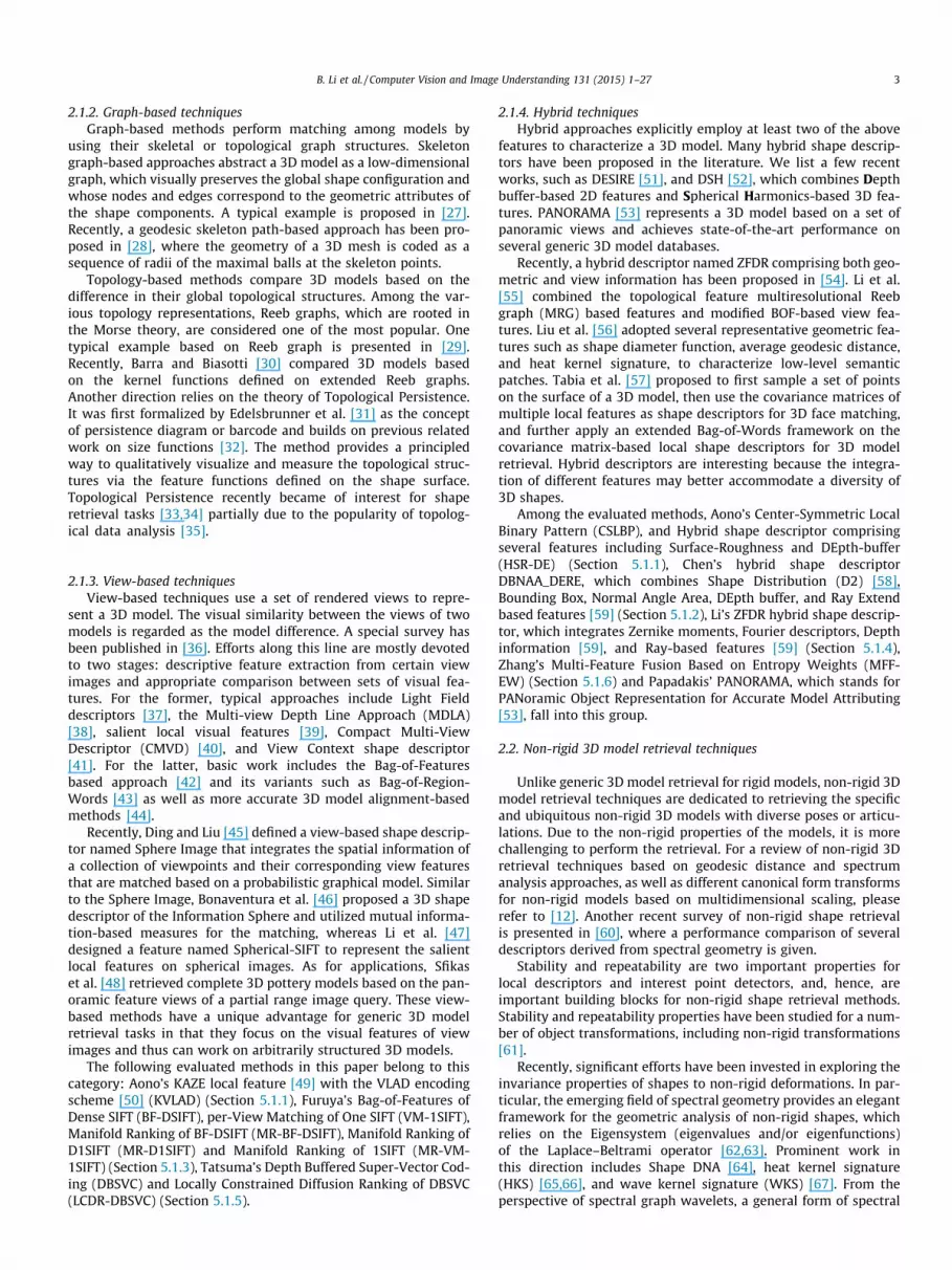
2.1.3. View-based techniquesView-based techniques use a set of rendered views to repre-

sent a 3D model. The visual similarity between the views of twomodels is regarded as the model difference. A special survey hasbeen published in [36]. Efforts along this line are mostly devotedto two stages: descriptive feature extraction from certain viewimages and appropriate comparison between sets of visual fea-tures. For the former, typical approaches include Light Fielddescriptors [37], the Multi-view Depth Line Approach (MDLA)[38], salient local visual features [39], Compact Multi-ViewDescriptor (CMVD) [40], and View Context shape descriptor[41]. For the latter, basic work includes the Bag-of-Featuresbased approach [42] and its variants such as Bag-of-Region-Words [43] as well as more accurate 3D model alignment-basedmethods [44].

Recently, Ding and Liu [45] defined a view-based shape descrip-tor named Sphere Image that integrates the spatial information ofa collection of viewpoints and their corresponding view featuresthat are matched based on a probabilistic graphical model. Similarto the Sphere Image, Bonaventura et al. [46] proposed a 3D shapedescriptor of the Information Sphere and utilized mutual informa-tion-based measures for the matching, whereas Li et al. [47]designed a feature named Spherical-SIFT to represent the salientlocal features on spherical images. As for applications, Sfikaset al. [48] retrieved complete 3D pottery models based on the pan-oramic feature views of a partial range image query. These view-based methods have a unique advantage for generic 3D modelretrieval tasks in that they focus on the visual features of viewimages and thus can work on arbitrarily structured 3D models.

The following evaluated methods in this paper belong to thiscategory: Aono’s KAZE local feature [49] with the VLAD encodingscheme [50] (KVLAD) (Section 5.1.1), Furuya’s Bag-of-Features ofDense SIFT (BF-DSIFT), per-View Matching of One SIFT (VM-1SIFT),Manifold Ranking of BF-DSIFT (MR-BF-DSIFT), Manifold Ranking ofD1SIFT (MR-D1SIFT) and Manifold Ranking of 1SIFT (MR-VM-1SIFT) (Section 5.1.3), Tatsuma’s Depth Buffered Super-Vector Cod-ing (DBSVC) and Locally Constrained Diffusion Ranking of DBSVC(LCDR-DBSVC) (Section 5.1.5).

2.1.4. Hybrid techniquesHybrid approaches explicitly employ at least two of the above

features to characterize a 3D model. Many hybrid shape descrip-tors have been proposed in the literature. We list a few recentworks, such as DESIRE [51], and DSH [52], which combines Depthbuffer-based 2D features and Spherical Harmonics-based 3D fea-tures. PANORAMA [53] represents a 3D model based on a set ofpanoramic views and achieves state-of-the-art performance onseveral generic 3D model databases.

Recently, a hybrid descriptor named ZFDR comprising both geo-metric and view information has been proposed in [54]. Li et al.[55] combined the topological feature multiresolutional Reebgraph (MRG) based features and modified BOF-based view fea-tures. Liu et al. [56] adopted several representative geometric fea-tures such as shape diameter function, average geodesic distance,and heat kernel signature, to characterize low-level semanticpatches. Tabia et al. [57] proposed to first sample a set of pointson the surface of a 3D model, then use the covariance matrices ofmultiple local features as shape descriptors for 3D face matching,and further apply an extended Bag-of-Words framework on thecovariance matrix-based local shape descriptors for 3D modelretrieval. Hybrid descriptors are interesting because the integra-tion of different features may better accommodate a diversity of3D shapes.

Among the evaluated methods, Aono’s Center-Symmetric LocalBinary Pattern (CSLBP), and Hybrid shape descriptor comprisingseveral features including Surface-Roughness and DEpth-buffer(HSR-DE) (Section 5.1.1), Chen’s hybrid shape descriptorDBNAA_DERE, which combines Shape Distribution (D2) [58],Bounding Box, Normal Angle Area, DEpth buffer, and Ray Extendbased features [59] (Section 5.1.2), Li’s ZFDR hybrid shape descrip-tor, which integrates Zernike moments, Fourier descriptors, Depthinformation [59], and Ray-based features [59] (Section 5.1.4),Zhang’s Multi-Feature Fusion Based on Entropy Weights (MFF-EW) (Section 5.1.6) and Papadakis’ PANORAMA, which stands forPANoramic Object Representation for Accurate Model Attributing[53], fall into this group.

2.2. Non-rigid 3D model retrieval techniques

Unlike generic 3D model retrieval for rigid models, non-rigid 3Dmodel retrieval techniques are dedicated to retrieving the specificand ubiquitous non-rigid 3D models with diverse poses or articu-lations. Due to the non-rigid properties of the models, it is morechallenging to perform the retrieval. For a review of non-rigid 3Dretrieval techniques based on geodesic distance and spectrumanalysis approaches, as well as different canonical form transformsfor non-rigid models based on multidimensional scaling, pleaserefer to [12]. Another recent survey of non-rigid shape retrievalis presented in [60], where a performance comparison of severaldescriptors derived from spectral geometry is given.

Stability and repeatability are two important properties forlocal descriptors and interest point detectors, and, hence, areimportant building blocks for non-rigid shape retrieval methods.Stability and repeatability properties have been studied for a num-ber of object transformations, including non-rigid transformations[61].

Recently, significant efforts have been invested in exploring theinvariance properties of shapes to non-rigid deformations. In par-ticular, the emerging field of spectral geometry provides an elegantframework for the geometric analysis of non-rigid shapes, whichrelies on the Eigensystem (eigenvalues and/or eigenfunctions)of the Laplace–Beltrami operator [62,63]. Prominent work inthis direction includes Shape DNA [64], heat kernel signature(HKS) [65,66], and wave kernel signature (WKS) [67]. From theperspective of spectral graph wavelets, a general form of spectral

4 B. Li et al. / Computer Vision and Image Understanding 131 (2015) 1–27

descriptors was presented in [68], which includes HKS and WKS asspecial cases. A classic work in shape retrieval applications is theShape Google algorithm [69], which aggregates spectral descriptorsbased on the Bag-of-Features framework. Later, as the spatial parti-tion version, an intrinsic spatial pyramid matching algorithm wasdeveloped in [70]. Despite the elegance and popularity of these spec-tral methods, they require the input 3D models to have a manifolddata structure, which is unrealistic for most models collected fromthe web. Therefore, extra preprocessing is generally needed toremesh the surfaces before feeding them into the framework.

2.3. Semantics-based 3D model retrieval techniques

Semantics-based 3D model retrieval techniques incorporatehigh-level semantic information of the query and/or 3D modelsinto the retrieval process to bridge the semantic gap existing in tra-ditional content-based 3D model retrieval techniques. A survey ofthree typical semantics processing techniques (relevance feedback,machine learning, and ontology) is presented in [71]. Typicalsemantics-based 3D retrieval approaches include relevance feed-back [72], semantic labeling [73], neural networks [74], supervised[75–78] or semi-supervised [79–81] learning, boosting [82], proto-types [83], autotagging [84], spectral clustering [85], manifoldranking [86], semantic tree [87], feature dimension reduction[88], semantic subspaces [89], class distances [54], semanticsannotation of 3D models [90], semantic correspondences [91],and sparse structure regularized ranking [92].

Recently, the attribute-based semantic approach has becomepopular and has demonstrated promising performance, such asmultiple shape indexes (attributes) [93] and attribute-augmentedsemantic hierarchy [94]. Gong et al. [95] proposed to use attributesignature (AS) and reference set signature (RSS) to perform seman-tic 3D model retrieval. They selected 11 attributes including sym-metry, flexibility, rectilinearity, circularity, dominant-plane, long,thin, swim, fly, stand with leg(s), and natural. They found that theirhigh-level semantic approaches (AS and RSS) can complement low-level features, and they non-trivially improve the retrieval perfor-mance when used in combination. They also mentioned that oneadvantage of their semantic features is the compactness (makingthem efficient for large-scale retrieval scenarios).

The following evaluated algorithms belong to this type: Aono’smachine learning-based method CSLBP⁄ (Section 5.1.1); the mani-fold ranking-based approaches, including Furuya’s MR-D1SIFT andMR-VM-1SIFT (Section 5.1.3) and Tatsuma’s LCDR-DBSVC(Section 5.1.5) Query-by-Model algorithms; and Furuya’s CDMR(Section 5.2.1) and Tatsuma’s SCMR-OPHOG (Section 5.2.3)Query-by-Sketch algorithms.

2.4. 3D model retrieval benchmarks

A recent overview of existing sketch-based 3D model retrievalbenchmarks is available in [10]. Hence, we mainly concentrateon the review of currently available generic or specialized 3Dmodel retrieval benchmarks for the Query-by-Model retrieval.

2.4.1. Generic 3D model retrieval benchmarksTo evaluate the performance of a generic 3D model retrieval

algorithm, researchers have built generic 3D model retrievalbenchmarks including: the Princeton Shape Benchmark (PSB) [7],the SHREC’12 Generic Track Benchmark (SHREC12GTB) [96], theToyohashi Shape Benchmark (TSB) [97], and the Konstanz 3DModel Benchmark (CCCC) [59].

2.4.2. Specialized 3D model retrieval benchmarksSpecialized 3D model retrieval benchmarks are dedicated to

testing the performance of a 3D model retrieval algorithm on a

particular type of 3D models, such as non-rigid, watertight, or pro-fessional. For example, the following specialized 3D benchmarksexist: the Watertight Model Benchmark (WMB) [98], the McGill3D Shape Benchmark (MSB) [99], Bonn’s Architecture Benchmark(BAB) [100], and the Engineering Shape Benchmark (ESB) [101].

Table 1 lists the basic classification information of the aboveeight benchmarks whereas Fig. 2 shows some example modelsfor the four specialized benchmarks. We selected these eightbenchmarks to create the 3D target dataset of our benchmark.

Aside from the above mentioned benchmarks, there are severalother benchmarks or 3D model resources that may have overlapwith the eight benchmarks we selected. They include: (1) generic3D model datasets like the National Taiwan University 3D modeldatabase (NTU) [37], the NIST dataset [102], the AIM@SHAPEShape Repository [103], and the SHREC contests datasets (genericretrieval tracks, 2006�2014) [104]; (2) specialized 3D modelretrieval benchmarks like the TOSCA [105] and SHREC contestsdatasets (non-rigid, watertight, textured 3D, CAD, protein, face,human, range scan or parts-based partial retrieval tracks,2006�2014) [104].

3. Benchmark

3.1. Motivation and considerations

The benchmark was motivated by the latest large collection ofhuman-drawn sketches built by Eitz et al. [6]. To explore humansketch recognition and how humans draw sketches, they collected20,000 human-drawn sketches, categorized into 250 classes, eachwith 80 sketches. This sketch dataset is exhaustive in terms ofthe number of object categories. Thus, we believe that a 3D modelretrieval benchmark based on their object categorizations will bemore comprehensive and appropriate than other currently avail-able 3D retrieval benchmarks to more objectively and accuratelyevaluate the real-world performance of a 3D model retrieval algo-rithm. In addition, the sketch dataset avoids the bias issue since itcontains the same number of sketches for every class, and thenumber of sketches for one class is also adequate for a large-scaleretrieval benchmark. Moreover, the sketch variation within oneclass is also sufficient.

SHREC13STB [5] has found 1258 relevant models for 90 of the250 classes from the PSB benchmark. However, it is neither com-plete nor large enough. 160 classes, i.e., the majority, have not beenincluded. Thus, we felt a new 3D model retrieval benchmark basedon Eitz et al.’s sketch dataset and SHREC13STB, but extended byfinding more models from other 3D data sources, was needed. Itis useful for the proper evaluation of sketch-based or modelquery-based 3D model retrieval algorithms, especially their scala-bility, which is very important in practice.

To this end, we built a unified large-scale benchmark support-ing both sketch and model queries by extending SHREC13STB bymeans of identifying and consolidating relevant models for the250 classes of sketches from the major prior 3D shape retrievalbenchmarks. When creating the benchmark, our target was to findmodels for as many of the 250 classes as possible, and, for eachclass, to find as many models as possible. These previous bench-marks have been compiled with different goals in mind and, todate, have not been considered in combination. Our work is thefirst to integrate them to form a new, larger benchmark corpusfor both Query-by-Model and Query-by-Sketch retrieval.

3.2. Building process

Based on the above considerations, to build up a better andmore comprehensive large-scale 3D retrieval benchmark, we

Table 1Classification information of the eight generic or specialized 3D model retrieval benchmarks.

Benchmarks Types Number of models Number of classes Average number of models per class

PSB Generic 907 (train) 90 (train) 10 (train)907 (test) 92 (test) 10 (test)

SHREC12GTB Generic 1200 60 20TSB Generic 10000 352 28CCCC Generic 473 55 9WMB Watertight (articulated) 400 20 20MSB Articulated 457 19 24BAB Architecture 2257 183 (function-based) 12 (function-based)

180 (form-based) 13 (form-based)ESB CAD 867 45 19

(a) ESB

(b) MSB

(c) WMB

(d) BAB

Fig. 2. Example 3D models in ESB, MSB, WMB and BAB datasets.

1 The large-scale 3D model retrieval benchmark (LSB) is available at http://www.itl.nist.gov/iad/vug/sharp/contest/2014/SBR/.

B. Li et al. / Computer Vision and Image Understanding 131 (2015) 1–27 5

extend the search to eight available benchmarks. To avoid addingreplicate models, aside from the PSB used in SHREC13STB, theother seven available 3D model benchmark sources we consideredinclude the SHREC12GTB, TSB, CCCC, WMB, MSB, BAB, and ESB, aslisted in Table 1.

We (one undergraduate student, one master student, oneresearcher with a master degree and one with a Ph.D. degree)adopted a voting scheme to classify models. For the classificationof each model, we obtained at least two votes. If these two votesagree with each other, we confirm that the classification is correct;otherwise, we performed a third vote to finalize the classification.During the building process, we only kept one model for themodels that have duplicate copies spanning different sourcedatasets.

In the end, we found 13680 sketches and 8987 models, classi-fied into 171 classes (for the remaining 79 classes we did not findrelevant models in the selected benchmarks), which substantiallyincrease the scale of the benchmark and form the currently largestunified retrieval benchmark. The average number of models in

each class is 53, which is also much more than any of the bench-marks in Table 1. This benchmark provides an important resourcefor the community of 3D model retrieval and will likely foster thedevelopment of practical Query-by-Model and Query-by-Sketch3D retrieval applications.

3.3. Unified large scale benchmark: LSB

Our extended large-scale 3D model retrieval benchmark (LSB)1

is motivated by the latest large collection of human-drawn sketchesbuilt by Eitz et al. [6] and the SHREC’13 Sketch Track Benchmark(SHREC13STB) [5]. The details of the benchmark are as follows.

3.3.1. 2D sketch datasetThe 2D sketch query set contains 13680 sketches (171 classes,

each with 80 sketches) from Eitz et al.’s [6] human sketch

6 B. Li et al. / Computer Vision and Image Understanding 131 (2015) 1–27

recognition dataset, each of which has relevant models in theselected 3D benchmarks. This sketch dataset was used as the 2Dquery sketch dataset in evaluating large scale sketch-based 3Dshape retrieval algorithms in the SHREC’14 track on large scalesketch-based 3D shape retrieval [2].

3.3.2. 3D model datasetIn total, the 3D model dataset of the LSB benchmark contains

8987 models classified into 171 classes. Each model is saved inthe ‘‘.OFF’’ format as a text file. This 3D dataset was used in evalu-ating Query-by-Model 3D shape retrieval algorithms in theSHREC’14 track on comprehensive 3D shape retrieval [1]. It wasalso used as the target 3D model dataset in evaluating sketch-based 3D shape retrieval algorithms in the SHREC’14 track onextended large scale sketch-based 3D shape retrieval [2].

3.3.3. Ground truthAll the sketches and models are categorized according to the

classifications in Eitz et al. [6] and the selected source benchmarks,respectively. In our classification and evaluation, we adopt theclass names from Eitz et al. [6].

3.3.4. Training and testing subsetsTo evaluate and compare the performance of both learning-

based and non-learning based Query-by-Sketch 3D model retrievalalgorithms, we randomly selected 50 sketches from each class fortraining and used the remaining 30 sketches per class for testing,while the 3D model dataset as a whole was used for both trainingand testing.

3.4. Properties of the LSB benchmark

Table 2 lists the correspondences between the target 3D modeldataset of LSB and its source benchmarks. The indexing and map-ping relationship between our models and their original names inthe source benchmarks, as well as and the name list of the 171classes are available on the websites [1,2]. The average numberof vertices per model is 5,233. Though, on average, the numberof models per class is 53, it ranges from only 1 (i.e., for the basket,cake, fire hydrant, giraffe, lion, owl, parking meter, parrot, penguin,tennis racket, and van classes) to more than 600 (i.e., the chair andtable classes have 632 and 601 models, respectively). The 79 clas-ses that we did not find relevant models for are listed in Table 3. Ascan be seen, quite a few of them are either only parts (i.e., arm, eye,mouth, foot, and feather), or less representative or common to see(i.e., angel, boomerang, crane, mermaid, and pretzel), or relativelyprofessional (i.e. harp, saxophone, and trombone). Therefore, the171 classes for which we have found relevant models in the eightmajor 3D benchmarks are more representative and, as a whole,cover the majority of normal objects that appear in our lives.

Note that in the area of image retrieval, benchmarks with mil-lions of image objects [106] are considered large-scale by currentstandards. Often, these image benchmarks are obtained by crawl-ing the web. In the 3D object case, compiling publicly availableobject repositories of large size is still a challenge. While a lot of

Table 2Composition of the 8987 target 3D models in terms of the eight generic or specialized 3D

Benchmarks Generic

PSB SHREC12GTB TSB

#Used models 1,371 940 4,617Used percentage 75.6% 78.3% 46.2%LSB percentage 15.3% 10.5% 51.4%Domain percentage 81.3%

3D content is available in private and commercial repositories,the number of unique 3D objects freely available on the web is lim-ited. Hence, million-sized 3D object benchmarks are not yet realis-tic. We therefore consider our LSB benchmark large in the sensethat it is based on freely available and carefully compiled content.Eventually, this situation may change due to wider availability andeasy-to-use 3D acquisition technology (see also Section 7).

3.5. Evaluation metrics

3.5.1. General evaluation metricsTo perform a comprehensive evaluation of a retrieval algorithm

based on either a sketch or model query, we employed seven com-monly used performance metrics [7,1,2] in Information RetrievalEvaluation that are also widely used in the 3D model retrieval field.They are Precision-Recall (PR) diagram, Nearest Neighbor (NN),First Tier (FT), Second Tier (ST), E-Measures (E), Discounted Cumu-lated Gain (DCG) [7], and Average Precision (AP) [54]. We havedeveloped code [1,2] to compute all of these metrics. Their mean-ing and definitions are listed below.

� Precision-Recall plot (PR): Assume there are n models in thedataset, precision P is to measure the accuracy of the rele-vant models among the top K (16 K 6 n) ranking results,while recall R is the percentage of the relevant class thathas been retrieved in the top K results.

� Nearest Neighbor (NN): NN is the precision of the top mostmodel.

� First Tier (FT): Assume there are C relevant models in thedatabase, FT is the recall of the top C � 1 (for Query-by-Model retrieval, excluding the query model itself) or thetop C (for Query-by-Sketch retrieval) retrieved models.

� Second Tier (ST): Similarly, ST is the recall of the top 2(C � 1)(for Query-by-Model retrieval) or the top 2C (for Query-by-Sketch retrieval) retrieved models.

� E-Measure (E): Since generally people are more interested inthe retrieval results on the first page, E-Measure is defined[7] to measure the composite retrieval performance of bothprecision and recall of the top 32 retrieved models (that is,the exact results that usually can be shown within one page),

E ¼ 21P þ 1

R

: ð1Þ

� Discounted Cumulated Gain (DCG): The positions where therelevant models appear in the retrieval list are importantsince people are more interested in the models in the frontpart of the list. DCG is therefore defined as the normalizedsummed weighted value about the positions of the relevantmodels. To compute DCG, the retrieval list R is first trans-formed into a vector G, where Gi ¼ 1 if Ri is a relevant model,otherwise Gi ¼ 0. Then, DCG is computed according to thefollowing equation:

model

CC

38804.

DCGi ¼G1 i ¼ 1;DCGi�1 þ Gi

lg2 i otherwise:

(

retrieval benchmarks: the number of used models and its percentages.

Non-rigid Professional

CC WMB MSB BAB ESB

2 44 367 1,239 27.8% 11.0% 80.3% 54.9% 3.1%

3% 0.5% 4.1% 13.8% 0.3%4.6% 14.1%

Table 3Seventy-nine remaining classes without relevant models in the selected benchmarks.

angel arm backpack bell binoculars boomerang bottle opener bulldozer cactus calculatorcanoe carrot cat cloud comb computer mouse crane machine crown donut envelopeeye feather flashlight foot frying pan grenade hamburger harp head phones hedgehoghot dog ipod lobster loudspeaker megaphone mermaid moon mosquito mouse (animal) mouthnose panda paper clip parachute pigeon pineapple pizza power outlet present pretzelpurse radio rainbow revolver rollerblades rooster Santa Claus saxophone snail snowboardsocks speed boat sponge bob squirrel strawberry streetlight sun swan T-shirt tigertomato toothbrush tractor trombone trousers trumpet walkie-talkie wheelbarrow zebra

B. Li et al. / Computer Vision and Image Understanding 131 (2015) 1–27 7

Finally, it is normalized by its optimum:

DCG ¼ DCGn

1þPC

j¼21

lg2 j

: ð2Þ

� Average Precision (AP): AP is used to measure the overallperformance. It is computed as the total area under thePrecision-Recall curve. Therefore, it combines both preci-sion and recall.

We need to mention that, for the seven metrics above, a highervalue indicates better performance.

3.5.2. Weighted evaluation metricsBesides the common definitions of the evaluation metrics, we

also have developed two weighted versions for the benchmarkby incorporating the model variations in each class. Basically, weuse the number of available models to define the model variation.We assume there is a linear correlation between the number ofavailable models in one class and the degree of variation of theclass. Therefore, we adopt a weight based on the number of modelsor its reciprocal to define each weighted performance metric.

The proportionally mp and reciprocally mr weighted metrics(m = NN/FT/ST/E/DCG/AP) are defined as follows.

mp ¼PM

i¼1ni �miPMi¼1ni

; ð3Þ

mr ¼PM

i¼11ni�miPM

i¼11ni

; ð4Þ

where M is the total number of model/sketch queries, ni is the sizeof the class to which the i-th query belongs, and mi is the non-weighted NN/FT/ST/E/DCG/AP metric value for the i-th query. mp

assigns bigger weights to the classes with more variations. In con-trast, mr highlights the overall performance in retrieving diverseclasses by assigning bigger weights to the classes with few mod-els/variations. It is also intended to avoid the bias on the perfor-mance evaluation because of the different number of models indifferent classes.

4. Contributors

The first five authors of this paper built the above benchmarkand organized the SHREC’14 tracks on the topics of large scalecomprehensive and sketch-based 3D model retrieval as well as thisfollow-up study. Information about the other contributors of thetwo tracks is listed next.

4.1. Query-by-Model retrieval

There are five groups who have successfully participated in theSHREC’14 Comprehensive 3D Shape Retrieval track. In total, theyhave submitted fourteen dissimilarity matrices. In addition, anew group (Zhang et al.) has contributed seven new methodsand the organizers also ran the PANORAMA [53] method on our

benchmark based on the publically available executable [107].Below are details about the contributors and their twenty-tworuns.

� CSLBP-Run-1, CSLBP-Run-2, CSLBP-Run-3, HSR-DE and KVLADsubmitted by Masaki Aono, Nihad Karim Chowdhury, HitoshiKoyanagi, and Ryuichi Kosaka from Toyohashi University ofTechnology, Japan (Section 5.1.1).

� DBNAA_DERE submitted by Qiang Chen and Bin Fang fromChongqing University, China (Section 5.1.2).

� BF-DSIFT, VM-1SIFT, MR-BF-DSIFT, MR-D1SIFT and MR-VM-1SIFT submitted by Takahiko Furuya and Ryutarou Ohbuchifrom the University of Yamanashi, Japan (Section 5.1.3).

� ZFDR submitted by Bo Li and Yijuan Lu from Texas State Uni-versity, USA; and Henry Johan from Fraunhofer IDM@NTU,Singapore (Section 5.1.4).

� DBSVC and LCDR-DBSVC submitted by Atsushi Tatsuma andMasaki Aono from Toyohashi University of Technology, Japan(Section 5.1.5).

� MSD, SDS, MFF-EW, SHELL, SECTOR, SECSHELL, and D2 submit-ted by Chaoli Zhang, Haisheng Li, and Yajuan Wan from theBeijing Technology and Business University, China(Section 5.1.6).

� PANORAMA [53] submitted by the organizers based on theresults from the publicly available executable [107].

4.2. Query-by-Sketch retrieval

Four groups have participated in the SHREC’14 track onExtended Large Scale Sketch-Based 3D Shape Retrieval. Twelverank list results (runs) for six different methods developed by fourgroups have been submitted. The participants and their runs arelisted next.

� BF-fGALIF, CDMR (rSM ¼ 0:1, a = 0.6), CDMR (rSM ¼ 0:1,a = 0.3), CDMR (rSM ¼ 0:05, a = 0.6), and CDMR (rSM ¼ 0:05,a = 0.3) submitted by Takahiko Furuya and Ryutarou Ohbu-chi from the University of Yamanashi, Japan (Section 5.2.1).

� SBR-VC (a = 1) and SBR-VC (a ¼ 12) submitted by Bo Li and Yij-

uan Lu from Texas State University, USA; Henry Johan fromFraunhofer IDM@NTU, Singapore; and Martin Burtscher fromTexas State University, USA (Section 5.2.2).

� OPHOG and SCMR-OPHOG submitted by Atsushi Tatsuma andMasaki Aono from Toyohashi University of Technology, Japan(Section 5.2.3).

� BOF-JESC (Words800_VQ), BOF-JESC (Words1000 _VQ), andBOF-JESC (FV_PCA32_Words128) submitted by ChangqingZou from the Chinese Academy of Sciences, China; HongboFu from the City University of Hong Kong, China; andJianzhuang Liu from Huawei Technologies Co. Ltd., China(Section 5.2.4).

To provide an even better overview of the twenty-six evaluated3D model retrieval algorithms, we classify them in Table 4 based

Table 4Classification of the twenty-six evaluated methods. When classifying Query-by-Sketch methods, we refer to [10] for ‘‘Feature type’’: local or global 2D feature. DFM: direct featurematching, BoW: Bag-of-Words, SVC: super-vector coding, BoF: Bag-of-Features, SL: supervised learning, MR: manifold ranking, LCDR: Locally Constrained Diffusion Ranking,CDMR: Cross-Domain Manifold Ranking.

Index Evaluated method Feature type Feature coding/matching Learning scheme Semantic information Section Reference(s)

Query-by-Model1 CSLBP Hybrid DFM No No Section 5.1.1 [108,109]2 HSR-DE Hybrid DFM No No Section 5.1.1 [110]3 KVLAD View-based DFM SL Yes Section 5.1.1 [49,50]4 DBNAA_DERE Hybrid DFM No No Section 5.1.2 [111]5 BF-DSIFT View-based BoW No No Section 5.1.3 [96,112,113]6 VM-1SIFT View-based DFM No No Section 5.1.3 [96,112]7 MR-BF-DSIFT View-based BoW MR No Section 5.1.3 [96,112–114]8 MR-D1SIFT View-based BoW + DFM MR No Section 5.1.3 [96,112–114]9 MR-VM-1SIFT View-based DFM MR No Section 5.1.3 [96,112,114]

10 ZFDR Hybrid DFM No No Section 5.1.4 [54]11 DBSVC View-based SVC No No Section 5.1.5 [115,116]12 LCDR-DBSVC View-based SVC MR (LCDR) No Section 5.1.5 [115–117]13 MFF-EW Hybrid DFM No Yes Section 5.1.6 [118,119,79]14 MSD Geometric DFM No No Section 5.1.6 [58]15 SDS Geometric DFM No No Section 5.1.6 [17]16 SHELL Geometric DFM No No Section 5.1.6 [17]17 SECTOR Geometric DFM No No Section 5.1.6 [17]18 SECSHELL Geometric DFM No No Section 5.1.6 [17]19 D2 Geometric DFM No No Section 5.1.6 [58]20 PANORAMA Hybrid DFM No No Section 2.1.4 [53]

Query-by-Sketch21 BF-fGALIF Local BoW No No Section 5.2.1 [120,10]22 CDMR Local BoW MR (CDMR) No Section 5.2.1 [120,10]23 SBR-VC Global DFM No No Section 5.2.2 [121,5,10]24 OPHOG Local DFM No No Section 5.2.3 [122]25 SCMR-OPHOG Local DFM MR (SCMR) No Section 5.2.3 [122,123,117]26 BOF-JESC Local BoF No No Section 5.2.4 [124–126]

8 B. Li et al. / Computer Vision and Image Understanding 131 (2015) 1–27

on the following taxonomy: type of feature (e.g., view-based, geo-metric, or hybrid), feature coding/matching methods (e.g., directfeature matching (DFM), Bag-of-Words (BoW) or Bag-of-Features(BoF) framework, super-vector coding (SVC), or sparse coding(SC)), learning scheme (e.g., manifold learning (MR), supervisedlearning (SL), unsupervised learning (USL), or deep learning (DL)),and semantic information (e.g., usage of classification or labelinformation). However, since 3D model retrieval methods havebecome more and more complex due to involvement of differentlocal/global/hybrid features, diverse feature coding methods andvarious machine learning strategies or semantic information arebeing used, making it difficult to provide both a descriptive and acompact taxonomy to classify and differentiate 3D model retrievalalgorithms.

We also need to mention that each method has some parametersettings, which can be found in the following section on methoddescription.

5. Methods

5.1. Query-by-Model retrieval methods

5.1.1. Hybrid shape descriptors CSLBP⁄, HSR-DE, and KVLAD, by M.Aono, N.K., Chowdhury, H. Koyanagi, and R. Kosaka

We have investigated accurate 3D shape descriptors over theyears for massive 3D shape datasets. In the Large Scale Compre-hensive 3D Shape Retrieval track, we have attempted to applythree different methods with five runs. Note that all the five runs,we apply pose normalization [85] as preprocessing.

For the first three runs, we applied CSLBP⁄, a hybrid shapedescriptor, composed of Center-Symmetric Local Binary Pattern(CSLBP) feature [108], Entropy descriptor [109], and optional ChainCode (CC). The difference between the three runs comes from thenumber of view projections and the existence of the optional CC:16 views for CSLBP in Run-1, 24 views for CSLBP in Run-2 and

Run-3, while no CC for Run-1 and Run-2 and CC addition in Run-3. CSLBP⁄ is computed by first generating depth buffer images frommultiple viewpoints for a given 3D shape object, then by analyzinggray-scale intensities to produce three-resolution level histograms(in our implementation, 256 � 256, 128 � 128, and 64 � 64), hav-ing 16 bins each, after segmenting each depth-buffer image intosub-images (16, 8, 4, respectively). In addition to CSLBP, we haveaugmented it with ‘‘Entropy’’, trying to capture the randomnessof surface shapes, resulting in CSLBP⁄.

For the fourth run, we applied HSR-DE, another hybrid shapedescriptor, composed of multiple Fourier spectra obtained by Hole,Surface-Roughness, Depth-buffer, Contour, Line, Circle, and Edgeimages, an extension to the method we published in [110]. Fig. 3illustrates the method adopted in Run-4.

For the fifth run, we applied KVLAD, a supervised learningmethod we developed by combining non-linear scale space [49]with the Vector of Locally Aggregated Descriptor (VLAD) [50]. Forthe training stage, we employ SHREC2011 data and generate a codebook of size 500, which is used for distance computation duringthe testing stage.

KVLAD is a combination of the KAZE local feature [49], which issupposed to be free from blurring along the sharp edge, with thelocation sensitive encoding scheme VLAD to produce ‘‘Visual Fea-tures’’, which was introduced by Jégou et al. [50]. VLAD differs fromthe histogram-based bag of visual words (BoVW) model in that itmaintains the residual vector during the encoding procedure ofvisual features. VLAD can be represented by the following formula:

vi ¼Xx2Ci

ðx� ciÞ; ð5Þ

where i ¼ 1;2; . . . ;K; ci is the centroid of the i-th cluster Ci, and x isa local feature in the cluster Ci. Each element of vector vi has thesame dimension of local features. Assume that we have d dimen-sional local features, then plain VLAD can be regarded as a d� Kdimensional matrix. Although Jégou et al. suggest that dimension

Fig. 3. An example of HSR-DE (Hole and Surface-Roughness descriptors with Depth-buffer and Edge features augmented) before conversion to Fourier spectra.

Fig. 4. DBNAA_DERE feature extraction procedure.

B. Li et al. / Computer Vision and Image Understanding 131 (2015) 1–27 9

reduction of plain VLAD works reasonably well, we keep all the dataas they are. The KVLAD visual feature is represented by thefollowing:

V � v1;v2; . . . ;vK½ �: ð6Þ

Dissimilarity computation is carried out such that we computeEuclidean distance between the visual features extracted from aquery and the visual features of each 3D model. Assume that avisual feature for a query is given by Q , and an arbitrary 3D modelis given by V. The distance or the dissimilarity between them iscomputed as follows:

distðQ ;VÞ ¼ffiffiffiffiffiffiffiffiffiffiffiffiffiffiffiffiffiffiffiffiffiffiffiffiffiffiffiffiffiffiffiffiffiffiffiffiffiffiffiffiffiffiffiffiffiffiffiffiffiffiXK

i¼1

Xd

j¼1ðQ i;j � Vi;jÞ2

r: ð7Þ

The search results computed from the above equation areranked in ascending order.

5.1.2. 3D model retrieval descriptor DBNAA_DERE, by Chen et al. [111]We propose a combined 3D model feature named DBNAA_DERE

which contains five different features: D2 [58], Depth Bufferimages (DE) feature, Ray Extent (RE) [59] feature, BoundingBox feature, and Normal Angle Area feature. Based on the analysison model surfaces, for each vertex we compute the mean angle andthe average area of its adjacent faces and then use them to form ajoint 2D histogram distribution, which we name Normal AngleArea feature. Then, we extract the D2 [58] feature and BoundingBox feature for each model, followed by linearly combining allthe three features together based on fixed weights to form a newfeature named D2 Bounding Box Normal Area feature (DBNAA)[111]. At last, we combine our DBNAA feature with Depth Buffer(DE) [59] and Ray Extent (RE) [59] features to build a more power-ful feature named DBNAA_DERE [111]. Fig. 4 shows the featureextraction procedure.

(1) DBNAA feature extraction. DBNAA comprises three compo-nents: D2 feature, Bounding Box feature and Normal AngleArea feature. The well-known D2 feature is first introducedby Osada et al. [58]. Here we use D2 as a component ofour combined feature, and choose the parameters as follows:N = 1024 samples and B = 1024 bins, which means we sam-ple N = 1024 sample points and divide the histogram into1024 bins. Finally, we have a 1024-dimensional vector torepresent each model.

Bounding Box feature of a model is extracted after applyingContinuous Principle Component Analysis (CPCA) [59] on itfor pose normalization.

L ¼ fZmax � Zmin;Ymax � Ymin;Xmax � Xming; ð8Þ

FBB ¼rankðL;1ÞrankðL;2Þ ;

rankðL;2ÞrankðL;3Þ

� �; ð9Þ

where Zmax/Zmin is the maximum/minimum value of the z-axis coordinates of all the vertices of the model. Similar arewith Ymax/Ymin and Xmax/Xmin. rankðÞ is a function to sort thevector in ascending order, rankðL;1Þ means the first numberin the sorted vector L. Finally, we get a two-dimensional vec-tor FBB to represent the Bounding Box feature of the model.NAA feature is based on the mean angle A and average area Sof each vertex,

A ¼ 1Nv j

Xfni ;njgFvj

ni � nj; ð10Þ

S ¼ 1Nvj

XNvj

i¼1

Si; ð11Þ

where Nv j is the number of adjacent faces of the j-th vertex.Fvj is a set of the normals of the adjacent faces of the j-thvertex, while ni/nj is the normal of face i/j. Si is the area ofthe i-th face, and S is the average area of the adjacent faces.An illustration to demonstrate the A and S joint distributioncan be found in [111]. After obtaining the mean angle A

Fig. 5.DSIFT a

10 B. Li et al. / Computer Vision and Image Understanding 131 (2015) 1–27

and average area S, we can use them to form a joint 2D dis-tribution histogram, where both A and S are divided into Nbins. N is empirically set to be 16. NAA feature is thereforean N⁄N feature matrix. According to our experiments, NAAfeature is suitable to differentiate models with similar D2features.After getting the above three types of features, we combinethe three features as below,

dDBNAA ¼ a dD þ b dB þ ð1� a� bÞ dNAA; ð12Þ

where a and b are set as follows: a = 0.65, and b = 0.15according to our experiments on the SHREC’12 Track: Generic3D Shape Retrieval [96] dataset. dD is a scalar, which meansthe ‘1-norm D2 distance of two models. dB and dNAA are theBounding Box and Normal Angle Area feature distance,respectively. We need to mention that when combining fea-tures we should first normalize different feature distances,which can be found in [111].

(2) DBNAA_DERE feature combination. Inspired by the ideaproposed in Li and Johan [54], we also integrate the DepthBuffer-based (DE) and Ray-Extent (RE) [59] features byadopting a similar framework as DBNAA:

dDBNAA DERE ¼ a dDBNAA þ b dDE þ ð1� a� bÞ dRE: ð13Þ

We set a = 0.3 and b = 0.35, which are similarly based on theexperiments on the SHREC’12 Track: Generic 3D ShapeRetrieval [96] dataset.

Since the label information for the test dataset of the bench-mark is assumed unknown for the purpose of benchmarking, ourclass information-based retrieval method is not applicable here.For more details about the shape descriptor computation, pleaserefer to [111].

5.1.3. Visual feature combination for 3D model retrieval, by T. Furuyaand R. Ohbuchi

Our algorithm is essentially the same as the one described in[96,112]. Fig. 5 illustrates overall processing flow of the algorithm.It starts with multi-viewpoint rendering of 3D models, followed byextraction of a global visual feature and a set of local visual fea-tures from an image rendered from a view. A distance between apair of 3D models is computed as a sum of distances learned fromtwo distinct features.

Our algorithm employs a view-based approach for it is able tocompare 3D models in almost any shape representations, e.g.,polygon soup, open mesh, or point cloud. A set of local featuresaggregated by using Bag-of-Features (BF) approach (BF-DSIFTbelow) is known to attain certain invariance against articulationof 3D shapes, e.g., bending of joints. Such a feature, however, isincapable of distinguishing differences among rigid shapes, e.g,pipes bent in U shape and in S shape. Thus, a fusion of an aggre-gated local feature, which is insensitive to deformation or articula-tion, with a global feature sensitive to global deformation andarticulation (VM-1SIFT below) could improve overall accuracy.

Two feature-adaptive distances computed from two visual features (BF-nd VM-1SIFT) are fused by summation.

5.1.3.1. Visual feature extraction. Our method first renders a 3Dmodel into range images from multiple viewpoints spaced uni-formly in solid angle space. For the SHREC’14 Comprehensive 3DShape Retrieval track, we used 42 viewpoints. Image resolutionfor each range image is 256 � 256 pixels. Then the algorithmextracts a set of local visual features, Dense SIFT (DSIFT) [113],from each range image. The algorithm also extracts a global visualfeatures, One SIFT (1SIFT) [112] from a range image.

For DSIFT visual feature extraction, we randomly and denselysample feature points on the range image with prior to concentratefeature points on or near 3D model in the image (see Fig. 6(b)).From each feature point sampled on the image, we extract SIFT[127], which is a multi-scale, rotation-invariant local visual fea-ture. The number of feature points per image is set to 300 as in[113], resulting in about 13 K DSIFT features per 3D model. Theset of dense local features are aggregated into a single feature vec-tor per 3D model by using the BF approach. We use the ERC-Treealgorithm [128] to accelerate both codebook learning (clusteringof local features) and vector quantization of local features intovisual words. A frequency histogram of vector-quantized DSIFTfeatures becomes a Bag-of-Features DSIFT, or BF-DSIFT feature vec-tor for the 3D model.

For 1SIFT extraction, we sample a feature point at the center ofthe range image and extract a SIFT feature from a large region cov-ering the entire 3D model (see Fig. 6(c)). The number of 1SIFT permodel is equal to the number of rendering viewpoints, i.e., 42. Notethat the set of 1SIFT features is not BF-aggregated but is comparedper-feature (i.e., per-view). Thus, the matching algorithm by using1SIFT is called per-View Matching 1SIFT (VM-1SIFT).

5.1.3.2. Distance computation. Our method uses two different dis-tance metrics for retrieval ranking; (1) fixed distance and (2) fea-ture-adaptive distance learned by using Manifold Ranking (MR)algorithm [114].

(1) Fixed distance. Symmetric version of Kullback–LeiblerDivergence (KLD) is used as fixed distance metric. KLD per-forms well when comparing a pair of probability distribu-tions, i.e., histograms. For the BF-DSIFT, the distancebetween a pair of 3D models xi; xj is equivalent to KLDbetween BF-DSIFT feature vectors of the two models (Eq.(14)). For the VM-1SIFT, the distance between a pair of 3Dmodels is calculated by using Eq. (15) where Nv is the num-ber of 1SIFT features per model and xip is 1SIFT featureextracted from the view p of 3D model xi.

dBF�DSIFTðxi;xjÞ ¼ dKLDðxi; xjÞ; ð14Þ

dVM�1SIFTðxi;xjÞ ¼XNv

p¼1

min16q6Nv

dKLDðxip;xjqÞ: ð15Þ

Feature-adaptive distance. To improve distance metric

(2)among 3D models, we compute feature-adaptive distanceson a manifold of 3D model features. To do so, we apply theMR algorithm to each of the BF-DSIFT feature manifold andthe VM-1SIFT feature manifold. For each feature, we firstgenerate a Nm � Nm affinity matrix W where Nm is the num-ber of 3D models (Nm ¼ 8987 for Query-by-Model retrievalon LSB) and Wij indicates similarity between a pair of 3Dmodels xi; xj. Wij is computed by using the followingequation,

dðxi ;xjÞ� �(

Wij ¼exp � r if i – j;

0 otherwise;

where d is fixed distance of either BF-DSIFT (Eq. (14)) orVM-1SIFT (Eq. (15)).

(a) Original SIFT [127] (b) DSIFT (c) 1SIFT

Fig. 6. Our method combines dense local visual feature (DSIFT) and global visual feature (1SIFT).

B. Li et al. / Computer Vision and Image Understanding 131 (2015) 1–27 11

We normalize W by computing S ¼ D�12WD�

12 where D is a diag-

onal matrix whose diagonal element is Dii ¼P

jWij.We use the following closed form solution for the MR to find

relevance values in F given ‘‘source’’ vector Y. In the source vectorY, an element corresponding to the query 3D model is set to 1 toserve as the source of diffusion, while the other elements corre-sponding to the database 3D models are set to 0. Fij is the relevancevalue between 3D models i and j. A higher relevance means ahigher similarity, or a smaller diffusion distance.

F ¼ ðI� aSÞ�1Y: ð16Þ

We add prefix ‘‘MR-’’ before the feature comparison method to indi-cate MR-processed algorithms (MR-BF-DSIFT and MR-VM-1SIFT).For parameters, we use r = 0.005 and a = 0.975 for MR-BF-DSIFT,and use r = 0.0025 and a = 0.9 for MR-VM-1SIFT. To furtherimprove retrieval accuracy, we combine diffusion distances of thetwo features. The diffusion distances of MR-BF-DSIFT and MR-VM-1SIFT are normalized and then summed with equal weight (MR-D1SIFT).

5.1.4. Hybrid shape descriptor ZFDR, by Li and Johan [54]The comprehensive 3D model dataset contains both generic and

professional (e.g. CAD and architecture models), rigid and non-rigid, articulated and non-articulated, watertight and non-water-tight models. Due to the variations in the types and robustnessconsiderations in retrieval performance, we employ the hybridshape descriptor ZFDR devised in [54] which integrates both visualand geometric information of a 3D model: Zernike moments andFourier descriptor features of 13 cube-based sample views; Depthinformation feature of 6 depth buffer views and Ray-based featuresbased on ray shooting from the center of the model to its farthestsurface intersection points. Visual information-based features (e.g.,Z and F) have good performance in characterizing some classes like‘‘sea animal’’, but for some other types of models like ‘‘car’’, depthbuffer-based features (e.g., D and R) are better [83]. We optimallyintegrate the above four different but complementary features toformulate the hybrid shape descriptor ZFDR to increase its differ-entiation power.

Fig. 7 illustrates the overview of the feature extraction process:3D model normalization mainly utilizing Continuous PrincipleComponent Analysis (CPCA) [59] and extraction of four componentfeatures Z, F, D and R. The details of the retrieval algorithm aredescribed as follows.

(1) View sampling. As a tradeoff between efficiency and accu-racy, the approach sets cameras on the 4 top corners, 3 adja-cent face centers and 6 middle edge points of a cube togenerate 13 silhouette views to represent a 3D model.

(2) Zernike moments and Fourier descriptors features (ZF).For each silhouette view, up to 10-th order Zernikemoments [129] (totally 35 moments) and first 10 centroid

distance-based Fourier descriptors [130] are computed torespectively represent the region-based and contour-basedvisual features of the silhouette views of the 3D model.

(3) Depth information and Ray-based features (DR). Toimprove the versatility of the descriptor in characterizingdiverse types of models, the depth buffer-based featureand ray-based with spherical harmonic representation fea-ture developed by Vranic [59] are integrated into the hybridshape descriptor. The executable files [59] are utilized toextract the 438-dimensional D and 136-dimensional Rfeatures.

(4) ZFDR hybrid shape descriptor distance. Scaled-‘1 (scalingeach component of two feature vectors by their respective‘1-norm before computing the summed component-wise ‘1

distance metric) [59] or Canberra distance (computing the‘1 component-wise distance between any two componentsof two feature vectors followed by normalizing it by theirsum, followed by summing all the component-wise dis-tances) [76] metric is first applied to measure the compo-nent distances dZ ; dF ; dD, and dR between two models. Then,the hybrid descriptor distance dZFDR is generated by linearlycombining the four component distances.

(5) Distance ranking and retrieval list output. Sort the hybriddistances between the query model and all the models in thedataset in ascending order and then list the modelsaccordingly.

Please refer to the original paper [54] for more details about thefeature extraction and retrieval process.

5.1.5. Unsupervised 3D model retrieval based on Depth BufferedSuper-Vector Coding and Locally Constrained Diffusion Ranking, by A.Tatsuma and M. Aono5.1.5.1. Depth buffered super-vector coding. We propose a new 3Dmodel feature known as Depth Buffered Super-Vector Coding(DBSVC), an approach categorized as a bag-of-features method[131,113]. DBSVC extracts 3D model features from rendered depthbuffer images using a super-vector coding method [115]. Fig. 8illustrates the generation of our proposed DBSVC feature. We firstapply Point SVD, a pose normalization method developed previ-ously by the authors [85]. Post pose normalization, we enclosethe 3D model with a unit geodesic sphere. From each vertex ofthe unit geodesic sphere, we render depth buffer images with300� 300 resolution, and a total of 38 viewpoints are defined.

After image rendering, we extract local features from eachdepth buffer image. The SURF-128 descriptor is a well-known localfeature vector with outstanding discrimination power [116]. TheSURF-128 descriptor outperforms the regular SURF descriptor,but it turns more sparse. Thus, we apply the power and the ‘2 nor-malization, which diminish the sparseness of the SURF-128descriptor, and call it the Power SURF descriptor. Moreover, we

Fig. 7. ZFDR feature extraction process [54].

Fig. 8. Overview of the Depth Buffered Super-Vector Coding.

12 B. Li et al. / Computer Vision and Image Understanding 131 (2015) 1–27

employ feature augmentation with patch coordinates [132]. ThePower SURF descriptors are extracted from 98� 98 pixel patchesarranged every 5 pixels.

To calculate DBSVC, we generate a codebook of visual words inadvance. The visual word is thus defined as the center of a clusterobtained by applying K-means clustering to the Power SURFdescriptors, which are extracted from 3D models in the trainingdataset prepared by removing the decimated and the duplicatedmodels from the NTU 3D Model Dataset (NMD) [37]. K-means clus-tering is performed with K ¼ 2048.

We calculate DBSVC with the codebook of K visual wordsv1; . . . ;vK . Given a set of local features x1; . . . ;xN extracted from a3D model, let aki ¼ 1 if xi is assigned to vk and 0 otherwise. For eachk ¼ 1; . . . ;K , we define,

bk ¼1N

XN

i¼1

aki; ð17Þ

ck ¼ cffiffiffiffiffibk

p; ð18Þ

uk ¼1ffiffiffiffiffibk

p XN

i¼1

akiðxi � vkÞ; ð19Þ

where c is a nonnegative constant and is chosen as 0.001 in ourimplementation. Then the DBSVC feature is obtained by,

fDBSVC ¼ ½c1;uT1; . . . ; cK ;uT

K �T: ð20Þ

To diminish the sparseness, the DBSVC feature is normalized usingthe power and the ‘2 normalization. We simply calculate the Euclid-ean distance for comparing DBSVC features between two 3Dmodels.

5.1.5.2. Locally constrained diffusion ranking. We calculate rankingscores using our modified manifold ranking algorithm. We usethe Locally Constrained Diffusion Process (LCDP) [117] for calculat-ing the affinity matrix in the manifold ranking algorithm [123], andcall this method Locally Constrained Diffusion Ranking (LCDR).LCDP aims at capturing the geometric structure of data manifolds,reducing the effect of noisy data points. Given a set of data pointsf1; . . . ; fn, the transition probability matrix on the k-nearest neigh-bor graph is defined by,

P ¼ T�1E; ð21Þ

where Eij ¼ expð�jjf i � f jjj2=r2Þ if f j belongs to the k-nearest neigh-bors of f i and Eij ¼ 0 otherwise, and Tii ¼

PjEij. Furthermore, LCDP

sets a high value to the transition probability between two datapoints if all the paths among their k-nearest neighbors are short.This property is implemented in the following update strategy,

Wðt þ 1Þ ¼ PWðtÞPT : ð22Þ

For the initial affinity matrix Wð0Þ, we use a symmetrically normal-ized affinity matrix, which is defined as

Wð0Þ ¼ Q�1=2AQ�1=2; ð23Þ

where Aij ¼ expð�jjf i � f jjj2=r2Þ and Qii ¼P

jAij.Our LCDR calculates ranking scores using the manifold ranking

algorithm with the affinity matrix W obtained by LCDP. Given acolumn vector y ¼ ½y1; . . . ; yn�

T with yi ¼ 1 if f i is a query andyi ¼ 0 otherwise, the ranking score vector r ¼ ½r1; . . . ; rn�T in LCDRis defined by,

r ¼ ðI � aMÞ�1y; ð24Þ

B. Li et al. / Computer Vision and Image Understanding 131 (2015) 1–27 13

where M ¼ D�1=2WD�1=2;Dii ¼P

jWij, and a 2 ½0;1Þ is a tuningparameter.

LCDR allows to calculate the ranking scores, which capturemore geometric structure of data manifolds than the conventionalmanifold ranking methods. However, LCDR requires much execu-tion time because of calculating the matrix product repeatedly.We fixed the LCDR parameters through preliminary experimentswith the Princeton Shape Benchmark [7]. We set k to 12;r to0:36;a to 0.99, and the maximum number of iterations to 10.

5.1.6. 3D shape retrieval based on MSD, SDS and MFF-EW, by C. Zhang,H. Li, Y. Wan

To accommodate the characteristics of the large-scale bench-mark dataset, we adopt two highly time-efficient geometry-basedretrieval algorithms, which are modified from Ankerst et al.’sShape Histogram algorithm [17] and Osada et al.’s Shape Distribu-tion (D2) algorithm (SD) [58]. In addition, to better represent thefeature of each category dataset, the multi-feature fusion methodbased on entropy weight is adopted.

5.1.6.1. Modified Shape Distribution (MSD). To enhance the perfor-mance of the SD, we modify the 3D normalization part in the pre-processing step, and construct a cubic spline interpolation curve torepresent the statistical shape distribution histogram.

(1) 3D model normalization and sampling. Firstly, we obtain amodel’s gravity center by accumulating the gravities of allthe faces on the surface of the 3D model. Then, we translatethe gravity center to the origin and scale the model to makethe radius of its bounding sphere to be 1. Consequently, theD2 distance feature value is compressed into the range of[0,2], which contributes to the scale invariance property ofour algorithm. Finally, we randomly sample 1024 samplepoints for each model. Fig. 9 shows examples.

(2) Cubic spline interpolation curve construction. To betterdescribe the statistical properties of a Shape Distributionhistogram, a cubic spline interpolation curve with 1026 con-trol points, instead of polynomial fitting or piecewise linearfunction [58], is used to represent the shape distribution.Some examples are listed in Fig. 10.

5.1.6.2. Shell-Distance-Sum (SDS) algorithm. 3D Shape Histogramalgorithm [17] can be broadly divided into three types: SHELL, SEC-TOR and SECSHELL. Our SDS is based on SHELL and makes animprovement in the step of constructing the shape histogram. Inour algorithm, we sum the distances between every point in eachof 120 bins and the gravity center of the model to represent thefeature of that bin, instead of counting the number of points fallinginto each bin. This improvement enables SDS to describe both the

Fig. 9. Example sample point set

location and the magnitude information of the vertices on a 3Dmodel. In addition, we normalize the 3D model first, as in the cor-responding steps described in MSD.

5.1.6.3. Multi-Feature Fusion Based on Entropy Weights (MFF-EW). Considering the complementarity between the candidatefeatures for fusion, we select the MSD and SDS features in ourmulti-feature fusion algorithm. We propose a novel multi-featurefusion algorithm by adaptively computing the fusion feature weightsusing entropy for each query, which is similar to [118,119].

(1) Information entropy calculation based on a query result.The theoretical basis of this step is to characterize the differ-entiation ability of a 3D shape feature based on the informa-tion entropy of its retrieval results. We need to mention thatthe classification information of the benchmark is alsoneeded in this step.

s for no

(1) For each query model q 2 U, where U represents the tar-get 3D model dataset, we obtain the top k retrieved mod-els Rf

qk when using the shape feature f. We set k = 10based on experimental results as well as by referring tothe approach in [79].

(2) Counting the number of models in the top k models thatbelong to the same category, denoted as Rf

qki, wherei ¼ 1;2; . . . n and n is the number of categories. Thenwe calculate the probability distribution of Rf

qki, denotedas fp1; p2; . . . ; pi; . . . ; png,

rmaliz

pi ¼Rf

qki

Rfqk

ð25Þ

(3) Computing the entropy of Rfqk,Xn

EðRfqkÞ ¼ �

i¼1

pi � log2pi: ð26Þ

(2) Calculating the weight of feature. Based on the analysis ofStep (1), a smaller entropy demonstrates that the corre-sponding 3D feature can better describe the models, andwe should assign a large weight for it. Therefore, we formu-late their relationship as follows,

Wfqk ¼

1� EðRfqkÞ

m�Pm

f¼1EðRfqkÞ

: ð27Þ

where m is the total number of the 3D features, andPmf¼1Wf

qk ¼ 1.

(3) Computing fusion dissimilarity distance. First, we normal-

ize each row of the dissimilarity distance matrices resultingfrom different features,

df 0 ði; jÞ ¼ df ði; jÞ �mini

maxi �mini; j ¼ 1;2; . . . ;n; ð28Þ

ed 3D models.

Fig. 10. Example cubic spline interpolation curves used to represent the Shape Distribution histograms.

14 B. Li et al. / Computer Vision and Image Understanding 131 (2015) 1–27

where df ði; jÞ and df 0 ði; jÞ are the pre-normalized and normalized dis-tances between model i and model j respectively, while maxi andmini are the maximum and minimum distances in the ith row.Finally, the fusion dissimilarity distance is,

Dfusionði; jÞ ¼Xm

f¼1

df 0 ði; jÞ �Wfqk: ð29Þ

In the experiments, we also provide the performance of our imple-mentations of the original D2, and three types of 3D Shape Histo-grams (SHELL, SECTOR and SECSHELL) as a baseline for reference.

Fig. 11. Feature comparison using Unsupervised Cross-Domain Manifold Ranking(CDMR).

5.2. Query-by-Sketch retrieval methods

5.2.1. Ranking on Cross-Domain Manifold for sketch-based 3D modelretrieval, by T. Furuya and R. Ohbuchi

To compare a hand-drawn sketch to a 3D model, most of exist-ing methods compare a sketch with a set of multi-view renderedimages of a 3D model. However, there is a gap between sketchesand rendered images of 3D models. As hand-drawn sketches con-tain ‘‘noise’’, such as shape abstraction, semantic influence, stylisticvariation, and wobbly lines, these sketches are often dissimilar torendered images of 3D models.

Our algorithm employs an unsupervised distance metric learn-ing to partially overcome the gap between sketches and 3D models[10,120]. Our algorithm called Cross-Domain Manifold Ranking, orCDMR [120], tries to bridge the gap between features extracted intwo heterogeneous domains, i.e., domain of sketches and domainof rendered images of 3D models. While the CDMR algorithm could

perform in either an unsupervised, semi-supervised, or supervisedmode, we use unsupervised CDMR in this paper.

Fig. 11 shows an overview of the CDMR. It first creates two sep-arate manifolds of features, i.e., a manifold of sketch features and amanifold of 3D model features. The feature manifolds are com-puted by using an algorithm best suited for each of the domains;BF-fGALIF [120] (slightly modified BF-GALIF [133]) is used to com-pare sketches and BF-DSIFT [113] is used to compare 3D models.These two feature manifolds are then inter-linked to form aCross-Domain Manifold (CDM) by using an algorithm capable ofsketch-to-3D comparison, that is, the BF-fGALIF. Using the CDM,similarity values between a sketch query and 3D models are

B. Li et al. / Computer Vision and Image Understanding 131 (2015) 1–27 15

computed by diffusing relevance on the CDM. The relevance origi-nates from the query, and it diffuses towards 3D models via edgesof the CDM by using a process identical to Manifold Ranking [123].The higher the relevance value of a 3D model, the closer it is to thequery.

Unlike previous sketch-to-3D model comparison algorithms,the CDMR tries to maintain manifolds of sketches and 3D models.This often positively contributes to ranking accuracy. Also, if alarge enough number of sketches and their inter-similarity valuesare available, the CDMR performs a form of automatic queryexpansion on the manifold of sketches.

5.2.1.1. Forming a cross domain manifold. A CDM is a graph, whosevertices are either sketches or 3D models. The CDM graph W isrepresented by a matrix having size ðNs þ NmÞ � ðNs þ NmÞ, whereNs and Nm are the number of sketches and 3D models in a databaserespectively. For Query-by-Sketch retrieval on LSB, Ns = 13680 andNm = 8987.

The element of the matrix W, i.e., Wij, indicates similaritybetween a sketch (or a 3D model) i and a sketch (or a 3D model)j. (For details, please refer to [120].) Distances are computed foreach pair of vertices i and j by using the feature comparison meth-ods i.e., BF-fGALIF and BF-DSIFT. The distances are then convertedinto similarities by using the following equation where dði; jÞ is thedistance between vertices i and j.

Wij ¼expð�dði; jÞ=rÞ if i – j;

0 otherwise:

�The parameter r controls diffusion of relevance value across the

CDM. We use different values rSS;rMM , and rSM to compute sketch-to-sketch similarity, 3D model-to-3D model similarity, and sketch-to-3D model similarity, respectively. These similarity values mustbe computed either by feature similarity or semantic similarity(if available).

As mentioned above, sketch-to-3D model comparison uses BF-fGALIF algorithm [10,120], which is a slightly modified version ofBF-GALIF [133]. BF-fGALIF compare a sketch and multi-view ren-dered images of a 3D model by using sets of Gabor filter-basedlocal features. A 3D model is rendered into Suggestive Contour(SC) [134] images from multiple viewpoints. The sketch imageand the SC images of the 3D model are rotation-normalized byusing responses of multi-orientation Gabor filters computed ofthe image. After normalizing for rotation, fGALIF features are den-sely extracted from the image. The set of fGALIF features are inte-grated into a feature vector per image by using Bag-of-Features(BF) approach. A BF feature of the sketch is compared against aset of per-view BF features of the 3D model to find a distancebetween the sketch and the 3D model.

For sketch-to-sketch comparison, BF-fGALIF features areextracted from the sketches. Unlike the BF-fGALIF for sketch-to-

View sampling

Viewpointentropy

3D visuacomplex

Shape

Query sketch

Retrieval S

Fig. 12. Overview of the SBR-VC algorithm: the first row is for the precom

3D model comparison, the BF-fGALIF for sketch-to-sketch compar-ison does not perform rotation normalization.

To compare 3D models, we use the BF-DSIFT [113] algorithm. Itis also a view-based algorithm. A set of multi-scale, rotation-invari-ant local visual features is densely extracted from multi-view ren-dered range images of a 3D model. The set of local visual features isthen BF-integrated per 3D model for comparison. A little moredetail on the BF-DSIFT is found in Section 5.1.3.

5.2.1.2. Ranking on the cross domain manifold. After generating Wrepresenting a CDM, Manifold Ranking (MR) algorithm [123] isapplied on W to diffuse relevance value over the CDM from aquery. We use the closed form of the MR (Eq. (30)) to find rele-vance values in F given ‘‘source’’ matrix Y. In Eq. (30), I is an iden-tity matrix and S is a symmetrically normalized matrix of W and ais a parameter. Fij is the relevance value of the 3D model j given thesketch i. A higher relevance means a smaller distance.

F ¼ ðI� aSÞ�1Y: ð30Þ

Using a naive algorithm, CDMR requires time complexityOððNs þ NmÞ2Þ for generating the CDM graph W and OððNs þ NmÞ3Þfor diffusing relevance over the CDM (Eq. (30)). As shown in theexperiments, computing CDMR is slower than other Query-by-Sketch retrieval algorithms. Among the parameters for the CDMR(i.e., rSS;rMM ;rSM and a), we fixed rSS to 0.02 and rMM to 0.005through preliminary experiments. For rSM and a), we tried the fol-lowing combinations of the parameters; (rSM;a) = (0.1, 0.6), (0.1,0.3), (0.05, 0.6), (0.05, 0.3).

5.2.2. Efficient sketch-based 3D model retrieval based on viewclustering and parallel shape context matching (SBR-VC) [121,5,10], byB. Li, Y. Lu, H. Johan, and M. Burtscher

The SBR-VC algorithm first clusters a set of sample views ofeach model into an appropriate number of representative viewsaccording to its visual complexity, which is defined as the view-point entropy distribution of its sample views. Next, a parallel rel-ative frame-based shape context (referred as relative shapecontext) matching [135] algorithm is employed to compute thedistances between a 2D sketch and the representative silhouetteviews of a 3D model. Before retrieval, the relative shape contextfeatures of the representative views of all 3D target models areprecomputed. Fig. 12 presents an overview of the algorithm, whichis described in more detail below.

5.2.2.1. Precomputation.(1) Viewpoint entropy-based adaptive view clustering. This

clustering is performed in four steps. For each 3D model,the first step computes the viewpoint entropy of 81 viewsthat are sampled by subdividing a regular icosahedron usingthe Loop subdivision [136] rule. The second step calculates

lity views number

assignment

Viewpoint entropy-based view clustering

context matching Ranking & output

tage:

putation whereas the second row is for the retrieval stage [5] [10].

16 B. Li et al. / Computer Vision and Image Understanding 131 (2015) 1–27

the viewpoint entropy-based 3D visual complexity for eachmodel. The mean and standard deviation entropies m and sof all sample views of each 3D model are computed first.The 3D visual complexity of each model is defined as

Fig. 13. Overview of the Overlapped Pyramid of HOG.

C ¼

ffiffiffiffiffiffiffiffiffiffiffiffiffiffiffiffiffiffibs2 þ bm2

2

s; ð31Þ

where bs and bm are the entropies s and m normalized relativeto their maximum and minimum over all the models. Hence,C 2 ½0;1�. This metric has the ability to quantitatively mea-sure the visual complexity difference between modelsbelonging to different categories. In the third step, the visualcomplexity C of a 3D model is utilized to determine the num-ber of representative views

Nc ¼ a � C � N0d e; ð32Þ

where a is a constant and N0 is the number of sample viewsfor each 3D model. N0 is 81 in the presented SBR-VC algo-rithm. For large-scale retrieval, a is chosen as 1 or 1

2, whichcorresponds to an average of 18.5 or 9.5 representative views,respectively, for each model in the dataset. The fourth stepapplies Fuzzy C-Means [137] view clustering to the view-point entropy values of the 81 sample views, together withtheir viewpoint locations, to generate the representativeviews for each model.

(2) Feature view generation. Outline feature views for the 2Dsketches and the 3D models are generated. In the 3D case,silhouette views are first rendered followed by outlinefeature extraction. In the 2D case, silhouette views are gen-erated based on binarization, Canny edge detection, closing(once), dilation (7 times in this case), and hole filling.

(3) Relative shape context computation. Rotation-invariantrelative shape context features [135] are extracted to repre-sent both sketches and sample views. 50 feature points areuniformly sampled for each outline feature view based oncubic B-Spline interpolation.

Fig. 14. Preprocessing steps of the Overlapped Pyramid of HOG.

5.2.2.2. Online retrieval. With a 2D query sketch, a target 3D data-base, and the precomputed relative shape context features of therepresentative views of each model, the online retrieval algorithmworks as follows.

(1) Sketch feature extraction. First, an outline feature view ofthe 2D sketch is generated. Then, its relative shape contextfeatures are computed in parallel within the following threesteps: outline magnitude computation, log-polar histogramgeneration and normalization.

(2) 2D-3D distance computation. The relative shape contextmatching is performed between the sketch and each repre-sentative view of a model and the minimum 2D-3D match-ing cost is chosen as the sketch-model distance. Thecomputation of 2D-3D distances between the sketch andall the 3D models is also performed in parallel.

(3) 2D-3D distance ranking. The sketch-model distances aresorted in ascending order and the models are rankedaccordingly.

SBR-VC (a ¼ 1) and SBR-VC (a ¼ 12) represent two runs of the

SBR-VC algorithm with corresponding a values. The 70x perfor-mance speedup achieved over the serial code [5] is mainly due tothe parallelization and code optimization of the relative shapecontext matching algorithm.

5.2.3. Unsupervised sketch-based 3D model retrieval based onOverlapped Pyramid of HOG and Similarity Constrained ManifoldRanking, by A. Tatsuma and M. Aono5.2.3.1. Overlapped Pyramid of HOG. We propose a new feature vec-tor known as Overlapped Pyramid of Histograms of OrientationGradients (OPHOG) which is an extended version of the Pyramidof Histograms of Orientation Gradients [122] proposed in the fieldof image classification. An overview of the proposed OPHOG isillustrated in Fig. 13. OPHOG divides an image into overlapped cellsby stages, and extracts an orientation histogram from each cell.

We perform preprocessing to a 3D model and a sketch imagebefore extracting OPHOG features as shown in Fig. 14. In the pre-processing of the 3D model, we generate depth buffer images with300� 300 resolution from the 102 viewpoints that are composedof the vertices of a unit geodesic sphere. To obtain a sketch-likeimage, we apply Laplacian filtering, thinning transformation andGaussian filtering to the depth buffer image. Similarly, in the pre-processing of the sketch image, we resize it to 300� 300 resolu-tion, and employ thinning transformation and Gaussian filtering.

After preprocessing, OPHOG divides a given image into cellsusing a regular sliding window determined by the spatial level.The window size w and stride size s are defined by the image sizeh and spatial level l as follows:

w ¼ h=2l; s ¼ w=2: ð33Þ

The OPHOG feature is obtained by concatenating all of the ori-entation histograms calculated for each cell. The orientation histo-gram is constructed by voting gradient magnitude to thecorresponding orientation bin. The gradient magnitude g and ori-entation h are defined as follows:

gðx; yÞ ¼ffiffiffiffiffiffiffiffiffiffiffiffiffiffiffiffiffiffiffiffiffiffiffiffiffiffiffiffiffiffiffiffiffiffiffiffiffiffiffiffiffiuxðx; yÞ2 þ uyðx; yÞ2

q; ð34Þ

hðx; yÞ ¼ tan�1 uxðx; yÞuyðx; yÞ

; ð35Þ

where,

(a) (b)

Fig. 15. Illustration for the junction-based extended shape context featuredescriptor. Two local patches on a junction of a query sketch and a model vieware shown in (a) and (b), respectively.

B. Li et al. / Computer Vision and Image Understanding 131 (2015) 1–27 17

uxðx; yÞ ¼ Lðxþ 1; yÞ � Lðx� 1; yÞ;uyðx; yÞ ¼ Lðx; yþ 1Þ � Lðx; y� 1Þ;

and Lðx; yÞ denotes the image value at pixel ðx; yÞ.Finally, to decrease the influence of the noise in a sketch image,

we transform the OPHOG feature vector into its rank order vectorand apply the ‘2 normalization.

During implementation, we set the number of histogram bins to40 and limit the number of levels to 3. For comparing a sketchimage to a 3D model, we calculate the minimum Euclidean dis-tance, which is denoted by the following equation:

dðs;mÞ ¼ mini¼1;���;102

jjfðsÞ � fðmÞi jj; ð36Þ

where fðsÞ is the feature vector of sketch image s, and fðmÞi denotesthe feature vector of the ith depth buffer image rendered from 3Dmodel m.

5.2.3.2. Similarity constrained manifold ranking. We also propose anextended manifold ranking method [123] constrained by the sim-ilarity between a sketch image and a 3D model. In the following,we call this method Similarity Constrained Manifold Ranking(SCMR).

Suppose we have feature vectors of 3D model f1; . . . ; fn. SCMRaims to assign to each feature vector f i a ranking score ri whichreflects the non linear structure of the data manifold. To reflectthe data relations represented with the affinity matrix W withinthe ranking scores, we defined the following cost function:

12

Xn

i;j¼1

riffiffiffiffiffiffiDiip � rjffiffiffiffiffiffi

Djj

p !2

Wij; ð37Þ

where Dii ¼P

jWij. To preserve the similarity between a querysketch-image and a target 3D model in the ranking score, we addthe following fitting constraint term:Xn

i¼1

ðri � ziÞ2; ð38Þ

where zi ¼ expð�dðs;miÞ2=r2Þ is the similarity between the querysketch-image and ith target 3D model.

The optimal ranking score is obtained by minimizing followingcost function:

JðrÞ ¼ 12

Xn

i;j¼1

riffiffiffiffiffiffiDiip � rjffiffiffiffiffiffi

Djj

p !2

Wij þ lXn

i¼1

ðri � ziÞ2; ð39Þ

where l > 0 is a regularization parameter. Differentiating JðrÞ withrespect to r and rearranging, we obtain

r ¼ ðI � aMÞ�1z; ð40Þ

where M¼D�1=2WD�1=2; r¼½r1; . . . ;rn�T; z¼½z1; . . . ;zn�T, and a2 ½0;1Þis a tuning parameter. Clearly, the matrix ðI�aMÞ�1 can be calcu-lated off-line. The ranking score can be obtained by simplematrix-based vector multiplication.

In SCMR, we use the DBSVC as the feature vector for a 3D model.Furthermore, we calculate the affinity matrix using the LCDP [117].We fixed the SCMR parameters through preliminary experimentswith the SHREC’13 Sketch Track Benchmark [5]. For the SCMR,we set r to 0.1 and a to 0.85. For the LCDP, we set the numberof nearest neighbors to 10, the Gaussian width to 0.45, and themaximum number of iterations to 10.

5.2.4. BOF-JESC based descriptor, by C. Zou, H. Fu, and J. LiuBOF-JESC follows the bag-of-features framework. It employs a

junction-based extended shape context to characterize the localdetails within the four concentric circles centered at the key points.

The motivation of the BOF-JESC descriptor comes from twoaspects: (1) the local patch centered at a junction takes intoaccount contour salience, hence can capture important cues forperceptual organization and shape discrimination, as discussed in[124], and (2) the local descriptor shape context [125] is tailoredfor the images in this work (i.e., the sketches or model views) sincethey only contain contours. It has been evaluated by [138] to havea high discrimination performance.

BOF-JESC extracts a global histogram for each image M (Mdenotes a binary image obtained from a query sketch/model viewin this work). Edge point location in a local patch of BOF-JESC isquantized into 40 bins as shown in Fig. 15 (i.e. the number ofpoints is recorded in each bin). In our experiments, the best perfor-mance is achieved by setting the radius of the log-polar coordinateto 0.075, 0.15, 0.25 and 0.35 of RM (RM ¼

ffiffiffiffiffiffiffiffiffiffiffiffiffiffiW Hp

where W and H isthe width and height of the bounding box of M). The circle with theshortest radius is divided into four bins, as shown in Fig. 15, whichis based on the fact that the bins with small areas are more sensi-tive to the statistics of the edge points.

The 40 dimensional local feature of BOF-JESC has the followingcharacteristics:

� BOF-JESC selects all the junctions (we uses the method in [124]to extract the junctions in M, and the points with degree one,e.g. the point p in Fig. 15(a), are also treated as junctions), andthe mid-points in the lines connecting two adjacent junctions(e.g. the point q in Fig. 15(a)) into the key-point set to generatelocal features.� BOF-JESC aligns the reference axis with h ¼ 0 of the log-polar

coordinate system to the average direction of the tangent linesof the ten nearest points in the longest edge connecting the cor-responding key-point, this step obtains a rotation invariance.� BOF-JESC quantizes the edge points on the boundary of two

neighboring bins into the bin with a greater angle (relative tothe reference axis in the anti-clockwise direction).� BOF-JESC normalizes a 40 dimensional local feature with‘1-norm regularization.

After the local features based on key-points are extracted fromall the model views in a database, BOF-JESC employs K-meansclustering to obtain d ‘‘visual words’’ and finally builds a global‘2-normalized histogram (i.e. a d dimensional feature vector) foreach model view in the off-line stage.

5.2.4.1. Implementation. We sample 42 views for each 3D modeluniformly on the unit viewpoint sphere. The vocabulary isobtained by the following steps: (1) concentrating the local fea-tures of all the model views in the database, (2) sampling 1 millionlocal features from concentrated features, (3) utilizing KNN to

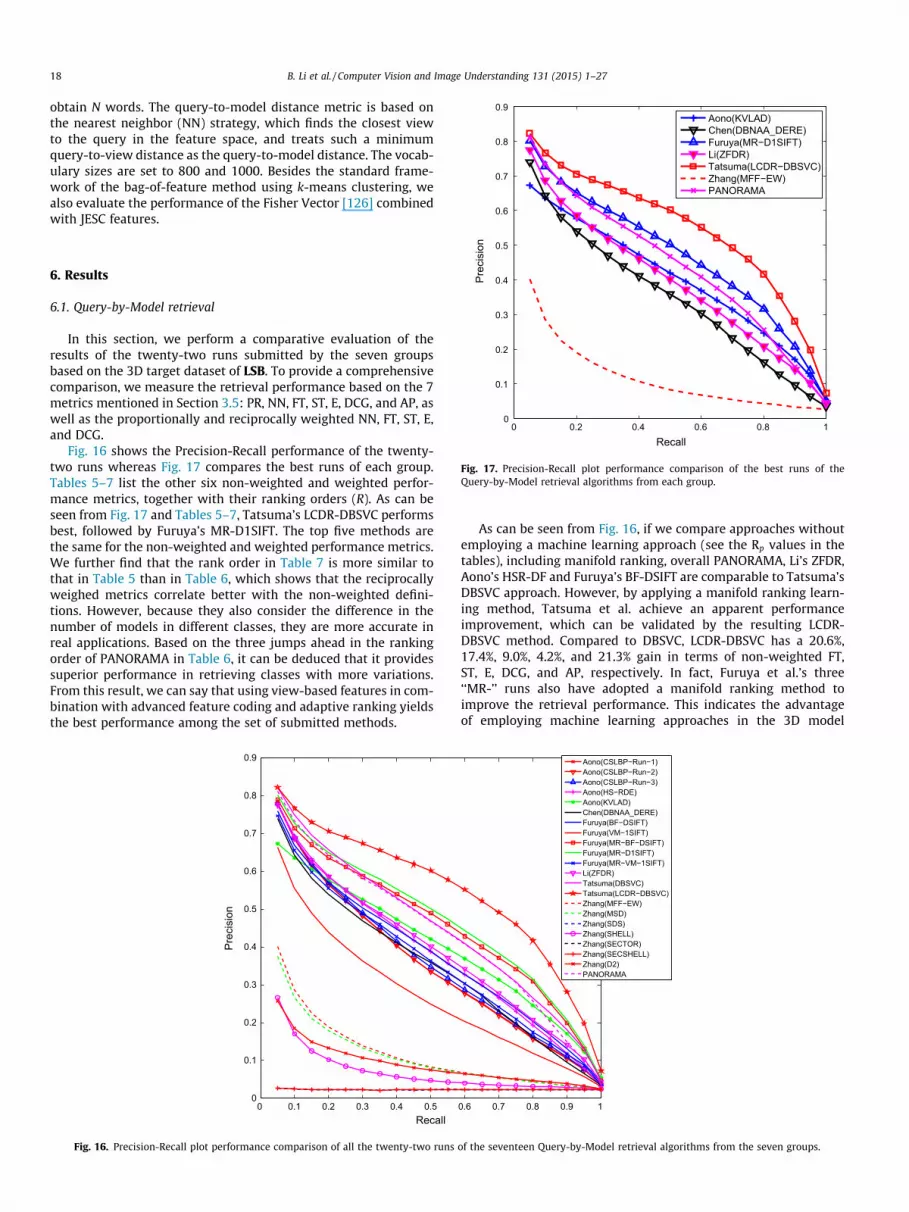
0.6

0.7

0.8

0.9Aono(KVLAD)Chen(DBNAA_DERE)Furuya(MR−D1SIFT)Li(ZFDR)Tatsuma(LCDR−DBSVC)Zhang(MFF−EW)PANORAMA

18 B. Li et al. / Computer Vision and Image Understanding 131 (2015) 1–27

obtain N words. The query-to-model distance metric is based onthe nearest neighbor (NN) strategy, which finds the closest viewto the query in the feature space, and treats such a minimumquery-to-view distance as the query-to-model distance. The vocab-ulary sizes are set to 800 and 1000. Besides the standard frame-work of the bag-of-feature method using k-means clustering, wealso evaluate the performance of the Fisher Vector [126] combinedwith JESC features.

0 0.2 0.4 0.6 0.8 10

0.1

0.2

0.3

0.4

0.5

Recall

Pre

cisi

onFig. 17. Precision-Recall plot performance comparison of the best runs of theQuery-by-Model retrieval algorithms from each group.

6. Results

6.1. Query-by-Model retrieval

In this section, we perform a comparative evaluation of theresults of the twenty-two runs submitted by the seven groupsbased on the 3D target dataset of LSB. To provide a comprehensivecomparison, we measure the retrieval performance based on the 7metrics mentioned in Section 3.5: PR, NN, FT, ST, E, DCG, and AP, aswell as the proportionally and reciprocally weighted NN, FT, ST, E,and DCG.

Fig. 16 shows the Precision-Recall performance of the twenty-two runs whereas Fig. 17 compares the best runs of each group.Tables 5–7 list the other six non-weighted and weighted perfor-mance metrics, together with their ranking orders (R). As can beseen from Fig. 17 and Tables 5–7, Tatsuma’s LCDR-DBSVC performsbest, followed by Furuya’s MR-D1SIFT. The top five methods arethe same for the non-weighted and weighted performance metrics.We further find that the rank order in Table 7 is more similar tothat in Table 5 than in Table 6, which shows that the reciprocallyweighed metrics correlate better with the non-weighted defini-tions. However, because they also consider the difference in thenumber of models in different classes, they are more accurate inreal applications. Based on the three jumps ahead in the rankingorder of PANORAMA in Table 6, it can be deduced that it providessuperior performance in retrieving classes with more variations.From this result, we can say that using view-based features in com-bination with advanced feature coding and adaptive ranking yieldsthe best performance among the set of submitted methods.

0 0.1 0.2 0.3 0.4 0.50

0.1

0.2

0.3

0.4

0.5

0.6

0.7

0.8

0.9

Recall

Pre

cisi

on

Fig. 16. Precision-Recall plot performance comparison of all the twenty-two runs

As can be seen from Fig. 16, if we compare approaches withoutemploying a machine learning approach (see the Rp values in thetables), including manifold ranking, overall PANORAMA, Li’s ZFDR,Aono’s HSR-DF and Furuya’s BF-DSIFT are comparable to Tatsuma’sDBSVC approach. However, by applying a manifold ranking learn-ing method, Tatsuma et al. achieve an apparent performanceimprovement, which can be validated by the resulting LCDR-DBSVC method. Compared to DBSVC, LCDR-DBSVC has a 20.6%,17.4%, 9.0%, 4.2%, and 21.3% gain in terms of non-weighted FT,ST, E, DCG, and AP, respectively. In fact, Furuya et al.’s three‘‘MR-’’ runs also have adopted a manifold ranking method toimprove the retrieval performance. This indicates the advantageof employing machine learning approaches in the 3D model

0.6 0.7 0.8 0.9 1

Aono(CSLBP−Run−1)Aono(CSLBP−Run−2)Aono(CSLBP−Run−3)Aono(HS−RDE)Aono(KVLAD)Chen(DBNAA_DERE)Furuya(BF−DSIFT)Furuya(VM−1SIFT)Furuya(MR−BF−DSIFT)Furuya(MR−D1SIFT)Furuya(MR−VM−1SIFT)Li(ZFDR)Tatsuma(DBSVC)Tatsuma(LCDR−DBSVC)Zhang(MFF−EW)Zhang(MSD)Zhang(SDS)Zhang(SHELL)Zhang(SECTOR)Zhang(SECSHELL)Zhang(D2)PANORAMA

of the seventeen Query-by-Model retrieval algorithms from the seven groups.

Table 5Performance metrics for the performance comparison of the twenty-two runs of the seventeen Query-by-Model retrieval algorithms from the seven groups. ‘‘R’’ denotes theranking order of all the twenty-two runs, while ‘‘Rp ’’ denotes the ranking order of all the runs that do not utilize any machine learning techniques or class information, that is, theruns of the pure shape descriptors themselves. Bold values indicate the best results.

Contributor Method NN FT ST E DCG AP R Rp

Aono CSLBP-Run-1 0.840 0.353 0.452 0.197 0.736 0.349 12 7CSLBP-Run-2 0.842 0.352 0.450 0.197 0.735 0.347 13 8CSLBP-Run-3 0.840 0.359 0.459 0.200 0.740 0.355 11 6HSR-DE 0.837 0.381 0.490 0.203 0.752 0.378 8 4KVLAD 0.605 0.413 0.546 0.214 0.746 0.396 6 –

Chen DBNAA_DERE 0.817 0.355 0.464 0.188 0.731 0.344 14 9

Furuya BF-DSIFT 0.824 0.378 0.492 0.201 0.756 0.375 9 5VM-1SIFT 0.732 0.282 0.380 0.158 0.688 0.269 15 10MR-BF-DSIFT 0.845 0.455 0.567 0.229 0.784 0.453 3 –MR-D1SIFT 0.856 0.465 0.578 0.234 0.792 0.464 2 –MR-VM-1SIFT 0.812 0.368 0.467 0.194 0.737 0.357 10 –

Li ZFDR 0.838 0.386 0.501 0.209 0.757 0.387 7 3

Tatsuma DBSVC 0.868 0.438 0.563 0.234 0.790 0.446 4 1LCDR-DBSVC 0.864 0.528 0.661 0.255 0.823 0.541 1 –

Zhang MFF-EW 0.566 0.138 0.204 0.076 0.570 0.114 16 –MSD 0.504 0.132 0.196 0.071 0.562 0.109 17 11SDS 0.486 0.074 0.114 0.041 0.511 0.023 20 14SHELL 0.483 0.078 0.119 0.043 0.513 0.069 19 13SECTOR 0.398 0.062 0.098 0.035 0.495 0.023 20 14SECSHELL 0.469 0.079 0.118 0.045 0.511 0.023 20 14D2 0.232 0.103 0.168 0.046 0.527 0.089 18 12

[53] PANORAMA 0.859 0.436 0.560 0.225 0.783 0.437 5 2

Table 6Proportionally weighted performance metrics for the performance comparison of the twenty-two runs of the seventeen Query-by-Model retrieval algorithms from the sevengroups. ‘‘R’’ denotes the ranking order of all the twenty-two runs, while ‘‘Rp ’’ denotes the ranking order of all the runs that do not utilize any machine learning techniques or classinformation, that is, the runs of the pure shape descriptors themselves. Bold values indicate the best results.

Contributor Method NN FT ST E DCG R Rp

Aono CSLBP-Run-1 0.880 0.379 0.502 0.145 0.800 11 7CSLBP-Run-2 0.881 0.375 0.495 0.145 0.798 13 9CSLBP-Run-3 0.878 0.381 0.505 0.146 0.802 10 6HSR-DE 0.882 0.405 0.539 0.148 0.812 6 3KVLAD 0.617 0.418 0.574 0.144 0.806 9 –

Chen DBNAA_DERE 0.859 0.398 0.544 0.136 0.799 12 8Furuya BF-DSIFT 0.868 0.392 0.529 0.143 0.809 7 4

VM-1SIFT 0.797 0.290 0.406 0.120 0.753 15 10MR-BF-DSIFT 0.877 0.464 0.607 0.156 0.834 5 –MR-D1SIFT 0.895 0.473 0.611 0.160 0.839 3 –MR-VM-1SIFT 0.868 0.388 0.501 0.142 0.798 13 –

Li ZFDR 0.879 0.398 0.535 0.148 0.809 7 4

Tatsuma DBSVC 0.898 0.444 0.604 0.162 0.839 3 2LCDR-DBSVC 0.892 0.541 0.723 0.169 0.872 1 –

Zhang MFF-EW 0.582 0.159 0.252 0.056 0.654 16 –MSD 0.544 0.157 0.249 0.054 0.652 17 11SDS 0.485 0.085 0.146 0.029 0.596 21 15SHELL 0.486 0.091 0.153 0.031 0.600 20 14SECTOR 0.446 0.071 0.124 0.028 0.587 22 16SECSHELL 0.503 0.091 0.150 0.034 0.601 19 13D2 0.281 0.139 0.234 0.038 0.632 18 12

[53] PANORAMA 0.891 0.472 0.636 0.158 0.840 2 1

B. Li et al. / Computer Vision and Image Understanding 131 (2015) 1–27 19

retrieval research field. We should mention that the above findingis consistent with the three types of metrics, including standard,proportionally, and reciprocally weighted ones.

To perform an approximate efficiency performance comparison,we asked the contributors to provide timing information in termsof average response time per query, as listed in Table 8. Obviously,ZFDR and BF-DSIFT are the most efficient ones, followed bythe Shape Histogram methods (SECTOR, SHELL, SECSHELL, SDS),MSD, MFF-EW, and VM-1SIFT, whereas the other methods aremuch slower. We also note that the best-performing methodLCDR-DBSVC is slower by an order of magnitude. This also raises

the issue of scalability of existing or new Query-by-Model retrievalalgorithms to large corpuses, and it deserves further efforts.

Among the seven group contributors, one group (Zhang) adoptsgeometry-based techniques, two groups (Furuya and Tatsuma) uti-lize view-based techniques, while four groups (Aono, Chen, Li, andPANORAMA [53]) follow a hybrid approach. If we consider theabove evaluation results as well, this demonstrates the popularityand superiority of hybrid techniques.

However, if we classify the contributing methods based on theproperties of the features used, we find that two groups (Aono andTatsuma) employ a local shape descriptor, four groups (Chen, Li,

Table 7Reciprocally weighted performance metrics for the performance comparison of the twenty-two runs of the seventeen Query-by-Model retrieval algorithms from the sevengroups. ‘‘R’’ denotes the ranking order of all the twenty-two runs, while ‘‘Rp ’’ denotes the ranking order of all the runs that do not utilize any machine learning techniques or classinformation, that is, the runs of the pure shape descriptors themselves. Bold values indicate the best results.

Contributor Method NN FT ST E DCG R Rp

Aono CSLBP-Run-1 0.663 0.303 0.359 0.180 0.571 10 7CSLBP-Run-2 0.668 0.304 0.359 0.180 0.571 10 7CSLBP-Run-3 0.658 0.310 0.365 0.183 0.573 9 6HSR-DE 0.656 0.318 0.380 0.189 0.582 8 5KVLAD 0.480 0.323 0.434 0.213 0.564 12 –

Chen DBNAA_DERE 0.626 0.281 0.339 0.169 0.552 14 9

Furuya BF-DSIFT 0.645 0.321 0.389 0.192 0.588 6 3VM-1SIFT 0.547 0.235 0.290 0.142 0.510 15 10MR-BF-DSIFT 0.680 0.376 0.444 0.221 0.619 4 –MR-D1SIFT 0.689 0.383 0.455 0.227 0.627 3 –MR-VM-1SIFT 0.626 0.300 0.359 0.179 0.564 12 –

Li ZFDR 0.659 0.326 0.392 0.194 0.588 6 3

Tatsuma DBSVC 0.707 0.371 0.445 0.224 0.628 2 1LCDR-DBSVC 0.718 0.428 0.506 0.255 0.658 1 –

Zhang MFF-EW 0.446 0.139 0.172 0.078 0.418 16 –MSD 0.395 0.124 0.157 0.070 0.400 17 11SDS 0.397 0.097 0.113 0.047 0.364 18 12SHELL 0.392 0.097 0.114 0.048 0.362 19 13SECTOR 0.300 0.063 0.080 0.035 0.327 22 16SECSHELL 0.370 0.095 0.111 0.047 0.357 20 14D2 0.160 0.069 0.102 0.046 0.338 21 15

[53] PANORAMA 0.687 0.350 0.421 0.210 0.612 5 2

Table 8Available timing information comparison of the seventeen Query-by-Model retrieval algorithms: T is the average response time (in seconds) per query. ‘‘R’’ denotes the rankingorder of all the seventeen runs, while ‘‘Rp ’’ denotes the ranking order of all the runs that do not utilize any machine learning techniques or class information, that is, the runs of thepure shape descriptors themselves. For PANORAMA [53], we collected the timing information based on the publically available executable [107]. Bold values indicate the bestresults.

Contributor (with computer configuration) Method Language T R Rp

Chen (CPU: Intel(R) Core i3–2350 M @2.3 GHz (only using one thread); Memory:6 GB; OS: Windows 2003 32-bit)

DBNAA_DERE C#, Matlab 58.82 11 10

Furuya (CPU: Intel(R) Core i7 3930 K @3.20 GHz, GPU: NVIDIA GeForce GTX 670(the programs ran on a single thread); Memory: 64 GB; OS: Ubuntu 12.04)

BF-DSIFT C++, CUDA 1.94 2 2VM-1SIFT C++ 9.60 10 9MR-BF-DSIFT C++, CUDA 65.17 13 –MR-VM-1SIFT C++, CUDA 65.87 14 –MR-D1SIFT C++, CUDA 131.04 15 –

Li (CPU: Intel(R) Xeon(R) CPU X5675 @3.07 GHz (2 processors, 12 cores);Memory: 20 GB; OS: Windows 7 64-bit)

ZFDR C/C++ 1.77 1 1

Tatsuma (CPU: Intel(R) Xeon(R) CPU E5–2630 @2.30 GHz (2 processors, 12cores); Memory: 64 GB; OS: Debian Linux 7.3)

DBSVC C++, Python 62.66 12 11

LCDR-DBSVC C++, Python 668.61 17 –

Zhang (CPU: Intel(R) Xeon(R) E5620 @ 2.40 GHz; Memory: 12.00 GB; OS:Windows 7 64-bit)

MFF-EW C++, Matlab 8.05 9 –MSD C++, Matlab 4.10 8 8SECSHELL C++, Matlab 3.48 4 4

(CPU: Intel(R) Core(TM) i5–2450 M @ 2.50 GHz; Memory: 2.45 GB; OS:Windows 7 32-bit)

SDS C++, Matlab 3.91 6 6SHELL C++, Matlab 3.65 5 5SECTOR C++, Matlab 3.29 3 3D2 C++, Matlab 4.00 7 7

[53] (CPU: Intel(R) Xeon(R) CPU X5675 @3.07 GHz (2 processors, 12 cores);Memory: 20 GB; OS: Windows 7 64-bit)

PANORAMA C++ 370.2 16 12

20 B. Li et al. / Computer Vision and Image Understanding 131 (2015) 1–27

Zhang, and PANORAMA [53]) adopt a global feature, and one group(Furuya) adopts both local and global features. The two groups(Tatsuma and Furuya) that extract local features have applied theBag-of-Words framework and K-means clustering on the local fea-tures. Within the submitted methods for Query-by-Model retrie-val, this shows the popularity of global shape descriptors and theBag-of-Words technique in dealing with local features.

6.2. Query-by-Sketch retrieval

This section presents a comparative evaluation of the twelveruns of the six methods submitted by the four groups based on

LSB. We measure the retrieval performance using the seven met-rics mentioned in Section 3.5: PR, NN, FT, ST, E, DCG, and AP.

As described in Section 3.3.4, the complete query sketch datasetis divided into ‘‘Training’’ and ‘‘Testing’’ datasets as needed bymachine learning-based retrieval algorithms. To provide completereference performance data for learning-based methods as well asnon-learning based approaches (including all of the six participat-ing methods), we evaluate the submitted results on the ‘‘Training’’,the ‘‘Testing’’, and the complete datasets. Fig. 18 compares their PRperformance, while Tables 9–10 compare the other six general andreciprocally weighted performance metrics on these threedatasets.

Furuya(BF−fGALIF)Furuya(CDMR (σSM=0.1, α=0.6))

Furuya(CDMR (σSM=0.1, α=0.3))

Furuya(CDMR (σSM=0.05, α=0.6))

Furuya(CDMR (σSM=0.05, α=0.3))

Li(SBR−VC (α=1))Li(SBR−VC (α=1/2))Tatsuma(OPHOG)Tatsuma(SCMR−OPHOG)Zou(BOF−JESC (Words800_VQ))Zou(BOF−JESC (Words1000_VQ))Zou(BOF−JESC(FV_PCA32_Words128))

Furuya(BF−fGALIF)Furuya(CDMR (σSM=0.1, α=0.6))

Furuya(CDMR (σSM=0.1, α=0.3))

Furuya(CDMR (σSM=0.05, α=0.6))

Furuya(CDMR (σSM=0.05, α=0.3))

Li(SBR−VC (α=1))Li(SBR−VC (α=1/2))Tatsuma(OPHOG)Tatsuma(SCMR−OPHOG)Zou(BOF−JESC (Words800_VQ))Zou(BOF−JESC (Words1000_VQ))Zou(BOF−JESC(FV_PCA32_Words128))

Furuya(BF−fGALIF)Furuya(CDMR (σSM=0.1, α=0.6))

Furuya(CDMR (σSM=0.1, α=0.3))

Furuya(CDMR (σSM=0.05, α=0.6))

Furuya(CDMR (σSM=0.05, α=0.3))

Li(SBR−VC (α=1))Li(SBR−VC (α=1/2))Tatsuma(OPHOG)Tatsuma(SCMR−OPHOG)Zou(BOF−JESC (Words800_VQ))Zou(BOF−JESC (Words1000_VQ))Zou(BOF−JESC(FV_PCA32_Words128))

Tatsuma(SCMR−OPHOG)Furuya(CDMR (σSM=0.05, α=0.6))

Li(SBR−VC (α=1))Zou(BOF−JESC (Words800_VQ))

Tatsuma(SCMR−OPHOG)Furuya(CDMR (σSM=0.05, α=0.6))

Li(SBR−VC (α=1))Zou(BOF−JESC (Words800_VQ))

Tatsuma(SCMR−OPHOG)Furuya(CDMR (σSM=0.05, α=0.6))

Li(SBR−VC (α=1))Zou(BOF−JESC (Words800_VQ))

0 0.1 0.2 0.3 0.4 0.5 0.6 0.7 0.8 0.9 10

0.05

0.1

0.15

0.2

0.25

Recall

Pre

cisi

on

(a) Training dataset

0 0.1 0.2 0.3 0.4 0.5 0.6 0.7 0.8 0.9 10

0.05

0.1

0.15

0.2

0.25

Recall

Pre

cisi

on

(b) Testing dataset

0 0.1 0.2 0.3 0.4 0.5 0.6 0.7 0.8 0.9 10

0.05

0.1

0.15

0.2

0.25

Recall

Pre

cisi

on

(c) Complete benchmark

0 0.2 0.4 0.6 0.8 10

0.05

0.1

0.15

0.2

0.25

Recall

Pre

cisi

on

(d) Training dataset (best runs)

0 0.2 0.4 0.6 0.8 10

0.05

0.1

0.15

0.2

0.25

Recall

Pre

cisi

on

(e) Testing dataset (best runs)

0 0.2 0.4 0.6 0.8 10

0.05

0.1

0.15

0.2

0.25

Recall

Pre

cisi

on

(f) Complete benchmark (best runs)

Fig. 18. Precision-Recall plot performance comparisons on different datasets of our LSB benchmark for the twelve runs of six Query-by-Sketch retrieval methods from thefour participating groups. Please note that the range of the precision axis is [0,0.25].

B. Li et al. / Computer Vision and Image Understanding 131 (2015) 1–27 21

Table 9Performance metrics comparison on different datasets of our LSB benchmark for the twelve runs of six Query-by-Sketch retrieval methods from the four participating groups. ‘‘R’’denotes the ranking order of all the twelve runs, while ‘‘Rp’’ denotes the ranking order of all the runs that do not utilize any machine learning techniques, that is, the runs of thepure shape descriptors themselves. Bold values indicate the best results.

Contributor Method NN FT ST E DCG AP R Rp

Training datasetFuruya BF-fGALIF 0.113 0.050 0.079 0.036 0.321 0.045 9 4

CDMR (rSM ¼ 0:1, a = 0.6) 0.069 0.046 0.074 0.031 0.308 0.048 7 –CDMR (rSM ¼ 0:1, a = 0.3) 0.104 0.055 0.087 0.039 0.324 0.053 5 –CDMR (rSM ¼ 0:05, a = 0.6) 0.085 0.058 0.094 0.040 0.325 0.060 2 –CDMR (rSM ¼ 0:05, a = 0.3) 0.109 0.057 0.090 0.041 0.329 0.055 4 –

Li SBR-VC (a = 1) 0.097 0.050 0.081 0.038 0.320 0.050 6 2SBR-VC (a ¼ 1

2) 0.094 0.047 0.077 0.035 0.316 0.046 8 3

Tatsuma OPHOG 0.158 0.066 0.097 0.051 0.340 0.060 2 1SCMR-OPHOG 0.158 0.118 0.172 0.078 0.375 0.132 1 –

Zou BOF-JESC (Words800_VQ) 0.107 0.043 0.068 0.031 0.312 0.042 10 5BOF-JESC (Words1000_VQ) 0.101 0.040 0.064 0.028 0.307 0.039 11 6BOF-JESC (FV_PCA32_Words128) 0.099 0.040 0.062 0.027 0.304 0.038 12 7

Testing datasetFuruya BF-fGALIF 0.115 0.051 0.078 0.036 0.321 0.044 9 4

CDMR (rSM ¼ 0:1, a = 0.6) 0.065 0.046 0.075 0.031 0.308 0.047 7 –CDMR (rSM ¼ 0:1, a = 0.3) 0.100 0.056 0.087 0.039 0.325 0.052 5 –CDMR (rSM ¼ 0:05, a = 0.6) 0.081 0.058 0.094 0.040 0.326 0.060 3 –CDMR (rSM ¼ 0:05, a = 0.3) 0.109 0.057 0.089 0.041 0.328 0.054 4 –

Li SBR-VC (a = 1) 0.095 0.050 0.081 0.037 0.319 0.050 6 2SBR-VC (a ¼ 1

2) 0.083 0.047 0.075 0.035 0.315 0.046 8 3

Tatsuma OPHOG 0.160 0.067 0.099 0.052 0.341 0.061 2 1SCMR-OPHOG 0.160 0.115 0.170 0.079 0.376 0.131 1 –

Zou BOF-JESC (Words800_VQ) 0.086 0.043 0.068 0.030 0.310 0.041 10 5BOF-JESC (Words1000_VQ) 0.082 0.038 0.062 0.027 0.304 0.037 11 6BOF-JESC (FV_PCA32_Words128) 0.089 0.038 0.060 0.026 0.302 0.036 12 7

Complete benchmarkFuruya BF-fGALIF 0.114 0.050 0.079 0.036 0.321 0.045 9 4

CDMR (rSM ¼ 0:1, a = 0.6) 0.068 0.046 0.074 0.031 0.308 0.048 7 –CDMR (rSM ¼ 0:1, a = 0.3) 0.102 0.055 0.087 0.039 0.324 0.053 5 –CDMR (rSM ¼ 0:05, a = 0.6) 0.084 0.058 0.094 0.040 0.325 0.060 3 –CDMR (rSM ¼ 0:05, a = 0.3) 0.109 0.057 0.090 0.041 0.329 0.054 4 –

Li SBR-VC (a = 1) 0.096 0.050 0.081 0.038 0.319 0.050 6 2SBR-VC (a ¼ 1

2) 0.090 0.047 0.077 0.035 0.316 0.046 8 3

Tatsuma OPHOG 0.159 0.066 0.098 0.051 0.341 0.061 2 1SCMR-OPHOG 0.158 0.117 0.171 0.078 0.376 0.132 1 –

Zou BOF-JESC (Words800_VQ) 0.099 0.043 0.068 0.031 0.311 0.042 10 5BOF-JESC (Words1000_VQ) 0.094 0.039 0.063 0.028 0.306 0.039 11 6BOF-JESC (FV_PCA32_Words128) 0.095 0.039 0.061 0.027 0.303 0.037 12 7

22 B. Li et al. / Computer Vision and Image Understanding 131 (2015) 1–27

As shown in the figure and tables, Tatsuma’s SCMR-OPHOG isthe best by a large margin, followed by their OPHOG and Furuya’sCDMR. Nevertheless, the overall performance of the top methodsfrom other groups are very close, while the closeness appearanceof the other methods in the Precision-Recall plots is partiallybecause of the distinct disparity between the best method and oth-ers. It appears that the other groups could catch up with OPHOG interms of overall performance (e.g., see the Rp values in Table 9, butafter employing the manifold ranking-based method SCMR, Tatsu-ma’s group achieved much better performance. For example, com-pared to OPHOG, SCMR-OPHOG achieves a gain of 77.3%, 74.5%,52.94%, 10.3%, and 116.4% in FT, ST, E, DCG, and AP, respectively.Compared to the performance obtained in the SHREC’12 andSHREC’13 sketch-based 3D model retrieval tracks [4]5, the perfor-mance of all approaches has decreased sharply due to the muchmore challenging data in the new LSB benchmark. In fact, thereis an additional drop when compared to the performance achievedby the evaluated Query-by-Model retrieval algorithms in Sec-tion 6.1, which again demonstrates the challenges and semanticgaps that exist in sketch-based 3D model retrieval. It also seemsworthwhile to pay more attention to scalability issues whendeveloping sketch-based 3D retrieval algorithms, especially for

large-scale retrieval applications. More details about the retrievalperformance with respect to different classes for each participatingmethod can be found on the SHREC’14 sketch track homepage [2].

For the proportionally weighted metrics, we find that theresults of the evaluated methods are very close. For example, theproportionally weighted (FT, ST, E, DCG, AP) of SBR-VC (a = 1) are1.0e�05⁄(1.25, 1.25, 1.25, 0.00, 3.75, 1.25), while for SCMR-OPHOG, they are 1.0e�05⁄(2.50, 1.25, 2.50, 1.25, 5.00, 1.25). Hence,the performance of the contributed methods in retrieving classeswith more variations/models is very close. If we consider the com-parison and analysis results of the three types of metrics based onthe Query-by-Model retrieval results in Section 6.1 as well, weregard the set of reciprocally weighted metrics as the more accu-rate and robust weighted version to evaluate either 2D or 3Dquery-based retrieval algorithms.

In addition, rather than having a consistent evaluation result asin the Query-by-Model retrieval algorithms evaluation, we findthere is some discrepancy in the case of sketch-based 3D retrievalevaluation: the ranking results of the methods are somehow differ-ent when based on the reciprocally weighted metrics. For example,if we compare the ranking results in Tables 9–10, we find the rank-ing order of OPHOG and CDMR (rSM ¼ 0:05, a = 0.3) to be flipped.

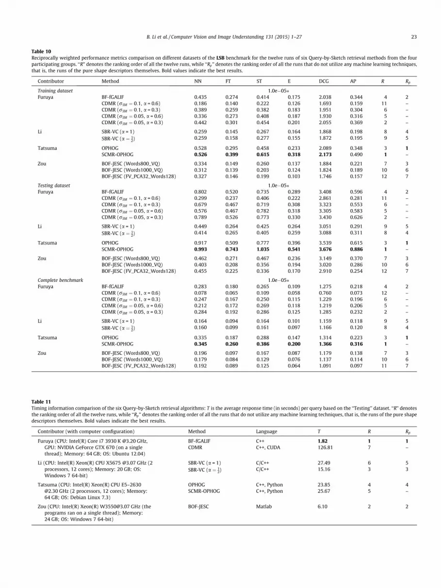
Table 10Reciprocally weighted performance metrics comparison on different datasets of the LSB benchmark for the twelve runs of six Query-by-Sketch retrieval methods from the fourparticipating groups. ‘‘R’’ denotes the ranking order of all the twelve runs, while ‘‘Rp ’’ denotes the ranking order of all the runs that do not utilize any machine learning techniques,that is, the runs of the pure shape descriptors themselves. Bold values indicate the best results.

Contributor Method NN FT ST E DCG AP R Rp

Training dataset 1.0e�05⁄Furuya BF-fGALIF 0.435 0.274 0.414 0.175 2.038 0.344 4 2

CDMR (rSM ¼ 0:1, a = 0.6) 0.186 0.140 0.222 0.126 1.693 0.159 11 –CDMR (rSM ¼ 0:1, a = 0.3) 0.389 0.259 0.382 0.183 1.951 0.304 6 –CDMR (rSM ¼ 0:05, a = 0.6) 0.336 0.273 0.408 0.187 1.930 0.316 5 –CDMR (rSM ¼ 0:05, a = 0.3) 0.442 0.301 0.454 0.201 2.055 0.369 2 –

Li SBR-VC (a = 1) 0.259 0.145 0.267 0.164 1.868 0.198 8 4SBR-VC (a ¼ 1

2) 0.259 0.158 0.277 0.155 1.872 0.195 9 5

Tatsuma OPHOG 0.528 0.295 0.458 0.233 2.089 0.348 3 1SCMR-OPHOG 0.526 0.399 0.615 0.318 2.173 0.490 1 –

Zou BOF-JESC (Words800_VQ) 0.334 0.149 0.260 0.137 1.884 0.221 7 3BOF-JESC (Words1000_VQ) 0.312 0.139 0.203 0.124 1.824 0.189 10 6BOF-JESC (FV_PCA32_Words128) 0.327 0.146 0.199 0.103 1.746 0.157 12 7

Testing dataset 1.0e�05⁄Furuya BF-fGALIF 0.802 0.520 0.735 0.289 3.408 0.596 4 2

CDMR (rSM ¼ 0:1, a = 0.6) 0.299 0.237 0.406 0.222 2.861 0.281 11 –CDMR (rSM ¼ 0:1, a = 0.3) 0.679 0.467 0.719 0.308 3.323 0.553 6 –CDMR (rSM ¼ 0:05, a = 0.6) 0.576 0.467 0.782 0.318 3.305 0.583 5 –CDMR (rSM ¼ 0:05, a = 0.3) 0.789 0.526 0.773 0.330 3.430 0.626 2 –

Li SBR-VC (a = 1) 0.449 0.264 0.425 0.264 3.051 0.291 9 5SBR-VC (a ¼ 1

2) 0.414 0.265 0.405 0.259 3.088 0.311 8 4

Tatsuma OPHOG 0.917 0.509 0.777 0.396 3.539 0.615 3 1SCMR-OPHOG 0.993 0.743 1.035 0.541 3.676 0.886 1 –

Zou BOF-JESC (Words800_VQ) 0.462 0.271 0.467 0.236 3.149 0.370 7 3BOF-JESC (Words1000_VQ) 0.403 0.208 0.356 0.194 3.020 0.286 10 6BOF-JESC (FV_PCA32_Words128) 0.455 0.225 0.336 0.170 2.910 0.254 12 7

Complete benchmark 1.0e�05⁄Furuya BF-fGALIF 0.283 0.180 0.265 0.109 1.275 0.218 4 2

CDMR (rSM ¼ 0:1, a = 0.6) 0.078 0.065 0.109 0.058 0.760 0.073 12 –CDMR (rSM ¼ 0:1, a = 0.3) 0.247 0.167 0.250 0.115 1.229 0.196 6 –CDMR (rSM ¼ 0:05, a = 0.6) 0.212 0.172 0.269 0.118 1.219 0.206 5 –CDMR (rSM ¼ 0:05, a = 0.3) 0.284 0.192 0.286 0.125 1.285 0.232 2 –

Li SBR-VC (a = 1) 0.164 0.094 0.164 0.101 1.159 0.118 9 5SBR-VC (a ¼ 1

2) 0.160 0.099 0.161 0.097 1.166 0.120 8 4

Tatsuma OPHOG 0.335 0.187 0.288 0.147 1.314 0.223 3 1SCMR-OPHOG 0.345 0.260 0.386 0.200 1.366 0.316 1 –

Zou BOF-JESC (Words800_VQ) 0.196 0.097 0.167 0.087 1.179 0.138 7 3BOF-JESC (Words1000_VQ) 0.179 0.084 0.129 0.076 1.137 0.114 10 6BOF-JESC (FV_PCA32_Words128) 0.192 0.089 0.125 0.064 1.091 0.097 11 7

Table 11Timing information comparison of the six Query-by-Sketch retrieval algorithms: T is the average response time (in seconds) per query based on the ‘‘Testing’’ dataset. ‘‘R’’ denotesthe ranking order of all the twelve runs, while ‘‘Rp ’’ denotes the ranking order of all the runs that do not utilize any machine learning techniques, that is, the runs of the pure shapedescriptors themselves. Bold values indicate the best results.

Contributor (with computer configuration) Method Language T R Rp

Furuya (CPU: Intel(R) Core i7 3930 K @3.20 GHz,GPU: NVIDIA GeForce GTX 670 (on a singlethread); Memory: 64 GB; OS: Ubuntu 12.04)

BF-fGALIF C++ 1.82 1 1CDMR C++, CUDA 126.81 7 –

Li (CPU: Intel(R) Xeon(R) CPU X5675 @3.07 GHz (2processors, 12 cores); Memory: 20 GB; OS:Windows 7 64-bit)

SBR-VC (a = 1) C/C++ 27.49 6 5SBR-VC (a ¼ 1

2) C/C++ 15.16 3 3

Tatsuma (CPU: Intel(R) Xeon(R) CPU E5–2630@2.30 GHz (2 processors, 12 cores); Memory:64 GB; OS: Debian Linux 7.3)

OPHOG C++, Python 23.85 4 4SCMR-OPHOG C++, Python 25.67 5 –

Zou (CPU: Intel(R) Xeon(R) W3550@3.07 GHz (theprograms ran on a single thread); Memory:24 GB; OS: Windows 7 64-bit)

BOF-JESC Matlab 6.10 2 2

B. Li et al. / Computer Vision and Image Understanding 131 (2015) 1–27 23

24 B. Li et al. / Computer Vision and Image Understanding 131 (2015) 1–27

The reciprocal version is to alleviate the bias influence due to thedifferences in the number of models that each class contains byproportionally weighting the performance per query by the reci-procal of the number of relevant models for the query. Therefore,it highlights the performance of classes with fewer models/varia-tions, which is usually even lower than the average performance.This results in the even smaller performance values in Table 10.We further find that this helps differentiate the performance ofthe various methods.

Similarly, we conducted an approximate efficiency evaluation.The average response time per query based on the ‘‘Testing’’ data-set using a modern computer is compared in Table 11. Obviously,BF-fGALIF is the most efficient, followed by BOF-JESC and SBR-VC(a ¼ 1

2). OPHOG, SCMR-OPHOG, and SBR-VC (a ¼ 1) are comparablein terms of speed, while CDMR is the slowest algorithm by an orderof magnitude. We believe this timing information is useful for anapproximate comparison of the runtime requirements of the algo-rithms even though they were obtained on different computers.

Finally, we classify all participating methods with respect to thetechniques employed according to the classification standardsdescribed in [10]: local/global 2D features, Bag-of-Words frame-work or direct feature matching, fixed/clustered views, and with/without view selection. Three groups (Furuya, Tatsuma, and Zou)utilize local features while one group (Li) employs a global feature.Two (Furuya and Zou) of the three methods based on local featuresapply the Bag-of-Features framework while manifold ranking isalso used in two (Furuya and Tatsuma) of the three local feature-based algorithms. Only one group (Li) performs view clusteringwhile the others employ a fixed view sampling. No group includesa view selection process in their methods.

7. Conclusions and future work

7.1. Conclusions

7.1.1. The LSB benchmarkThis paper describes the building process of LSB, a large-scale

3D model retrieval benchmark supporting both 3D model and 2Dsketch queries. Compared to other multimodal query-supported3D retrieval benchmarks, its 13680 sketches and 8987 models of171 classes make it the currently largest scale benchmark in termsof the number of models and sketches as well as the most compre-hensive benchmark in terms of the number of object classes andvariations within a class. Compared to previous sketch-based 3Dretrieval benchmarks, it is not only the largest and most compre-hensive but also the only currently available comprehensive 3Dmodel benchmark. Even compared to prior generic benchmarks,it is still among the largest and most comprehensive in terms ofthe number of categories. In addition to the LSB benchmark, wealso developed two versions of commonly used performance met-rics, proportionally-weighted and reciprocally-weighted, by incor-porating the model variations in each class based on the number ofavailable models it contains. We regard the reciprocally-weightedversion as more accurate than its original form in terms of reflect-ing the real performance of a 3D shape retrieval algorithm eitherusing model or sketch queries. We also hope that the large-scalesketch retrieval benchmark will prove useful for other researchersin our community.

7.1.2. Evaluation of Query-by-Model retrieval algorithmsBased on the 3D model dataset of the LSB benchmark, we orga-

nized the SHREC’14 large scale comprehensive 3D model retrievaltrack. In this paper, a comprehensive evaluation of twenty (twelvetrack participating and eight state-of-the-art or new) Query-by-Model retrieval algorithms has been conducted based on both

non-weighted and weighted performance metrics. A comparisonof approximate runtime information was also performed to pro-vide a reference on the efficiency of the evaluated methods, whichalso serves as evaluation of the scalability of each method w.r.tlarge-scale retrieval scenarios or real applications. According tothe evaluation results, among the submitted algorithms, hybridmethods, manifold ranking learning methods, and Bag-of-Wordsapproaches are more popular and promising in the scenario ofQuery-by-Model retrieval, which partially illustrates a currentresearch trend in the field of comprehensive 3D model retrieval.

7.1.3. Evaluation of Query-by-Sketch retrieval algorithmsBased on the complete LSB benchmark, we organized another

SHREC’14 track on large scale sketch-based 3D retrieval. The secondtrack is meant to foster this challenging and interesting researchdirection, encouraged by the success of the SHREC’12 and SHREC’13sketch-based 3D shape retrieval tracks. Though the latest bench-mark is by far the most challenging so far, we still attracted fourgroups who have successfully participated in the track and contrib-uted twelve runs of six methods, which have been comparativelyevaluated in this paper as well. We have noticed that the obtainedretrieval performance is far from satisfactory, and the performanceof existing sketch-based retrieval methods apparently drops whenscaled to a significantly larger collection. Local feature and manifoldranking based approaches also dominate the evaluated methods andoften achieve superior retrieval accuracy, but their performanceleaves room for further improvements.

7.2. Future work

The LSB benchmark provides a common platform to evaluate3D model retrieval approaches in the context of a large-scaleretrieval scenario. It helps identify state-of-the-art methods as wellas future research directions in this area. For promising futurework on sketch-based 3D retrieval algorithms, please refer to[10]. Here, we mainly list several important research directionsthat apply to both sketch and model query based 3D retrievalalgorithms.

� Benchmark. Since the current version of our LSB bench-mark contains only 171 of the full set of 250 classes fromEitz et al.’s sketch dataset, there is still room for furtherimprovement by finding models from additional sourcessuch as the Trimble 3D Warehouse (formerly the Google3D Warehouse) [139], to make it more complete and com-prehensive in terms of class variations. In addition, makingeach class contain the same number of sketches/modelswill help eliminate any bias, which we currently cope withusing the weighted metrics.

� Increasing amounts of 3D data. We expect that in thefuture, even more 3D object data will become available,due to technical advantages of 3D acquisition devices,cloud services and social media networks. In particular,the latter may include large amounts of noisy data, e.g.,from handheld and mobile devices. Then, the problem toretrieve among sets of 3D data of varying quality propertieswill become a challenge. Compiling benchmarks that con-trol for varying levels of quality of the 3D models will behelpful to foster research in this direction.

� Scalability of retrieval algorithms. Building scalable 3Dretrieval systems is of utmost importance for related inter-active applications. For Query-by-Sketch retrieval, animportant direction for future research in this area is todevelop more robust algorithms that scale to different sizesand diverse types of sketch queries and models. For Query-by-Model retrieval, though the performance is relatively

B. Li et al. / Computer Vision and Image Understanding 131 (2015) 1–27 25

speaking much better, it still requires further effort todevelop an interactive system for existing or new retrievalalgorithms w.r.t a large corpus by adopting additional tech-niques, such as parallelization (i.e., using multi-core CPUsor GPUs), as well as algorithm and code optimizations.

� Feature coding. Among the main parameters of 3D retrie-val algorithms, the coding of features has recently comeinto the focus of researchers. Techniques like sparse coding,Fisher coding, VLAD coding, etc. may provide for both effi-cient and effective retrieval. More systematic studies areneeded to assess the contribution of specific coding tech-niques to the overall method performance. In particular,it would be interesting to study if particular codings couldbe recommended for particular types of 3D features.

� Semantics-based 3D retrieval. As we saw, manifold learn-ing and attribute-based semantic retrieval approaches havebecome more and more important to bridge the gap in thepure content-based 3D model retrieval framework toachieve satisfactory accuracy. Therefore, we recommendutilizing techniques from other related disciplines, suchas machine learning, especially representation learning[140] including manifold learning and deep learning (i.e.,Caffe [141]), image retrieval (i.e., ImageNet [142]), and pat-tern recognition (i.e., [143], to develop higher level knowl-edge-based 3D retrieval algorithms.

Acknowledgments

The work of Bo Li and Yijuan Lu is supported by the Texas StateUniversity Research Enhancement Program (REP), Army ResearchOffice grant W911NF-12-1-0057, and NSF CRI 1305302 to Dr. Yiju-an Lu.

Henry Johan is supported by Fraunhofer IDM@NTU, which isfunded by the National Research Foundation (NRF) and managedthrough the multi-agency Interactive & Digital Media ProgrammeOffice (IDMPO) hosted by the Media Development Authority of Sin-gapore (MDA).

We would like to thank Yuxiang Ye and Natacha Feola whohelped us build the LSB benchmark.

We would like to thank Mathias Eitz, James Hays and MarcAlexa who collected the 250 classes of sketches. We would also liketo thank the following authors for building the 3D benchmarks:

� Philip Shilane, Patrick Min, Michael M. Kazhdan, and Tho-mas A. Funkhouser who built the Princeton Shape Bench-mark (PSB).

� Atsushi Tatsuma, Hitoshi Koyanagi, and Masaki Aono whobuilt the Toyohashi Shape Benchmark (TSB).

� Dejan Vranic and colleagues who built the Konstanz 3DModel Benchmark (CCCC).

� Daniela Giorgi who built the Watertight Shape Benchmark(WMB).

� Kaleem Siddiqi, Juan Zhang, Diego Macrini, Ali Sho-koufandeh, Sylvain Bouix, and Sven Dickinson who builtthe McGill 3D Shape Benchmark (MSB).

� Raoul Wessel, Ina Blümel, and Reinhard Klein from the Uni-versity of Bonn and the TIB Hannover who built the BonnArchitecture Benchmark (BAB).

� Subramaniam Jayanti, Yagnanarayanan Kalyanaraman,Natraj Iyer, and Karthik Ramani who built the EngineeringShape Benchmark (ESB).

References

[1] http://www.itl.nist.gov/iad/vug/sharp/contest/2014/Generic3D/, 2014.[2] http://www.itl.nist.gov/iad/vug/sharp/contest/2014/SBR/, 2014.

[3] A.-P. Ta, C. Wolf, G. Lavoué, A. Baskurt, 3D object detection and viewpointselection in sketch images using local patch-based Zernike moments, in:S.D. Kollias, Y.S. Avrithis (Eds.), CBMI, IEEE Computer Society, 2009, pp.189–194.

[4] B. Li, T. Schreck, A. Godil, M. Alexa, T. Boubekeur, B. Bustos, J. Chen, M. Eitz, T.Furuya, K. Hildebrand, S. Huang, H. Johan, A. Kuijper, R. Ohbuchi, R. Richter,J.M. Saavedra, M. Scherer, T. Yanagimachi, G.-J. Yoon, S.M. Yoon, SHREC’12track: sketch-based 3D shape retrieval, in: Eurographics Workshop on 3DObject Retrieval (3DOR), 2012, pp. 109–118.

[5] B. Li, Y. Lu, A. Godil, T. Schreck, M. Aono, H. Johan, J.M. Saavedra, S. Tashiro,SHREC’13 track: large scale sketch-based 3D shape retrieval, in: EurographicsWorkshop on 3D Object Retrieval (3DOR), 2013, pp. 89–96.

[6] M. Eitz, J. Hays, M. Alexa, How do humans sketch objects?, ACM Trans Graph.31 (2012) 44:1–44:10.

[7] P. Shilane, P. Min, M.M. Kazhdan, T.A. Funkhouser, The Princeton shapebenchmark, in: SMI, 2004, pp. 167–178.

[8] B. Li, Y. Lu, C. Li, A. Godil, T. Schreck, M. Aono, M. Burtscher, H. Fu, T. Furuya, H.Johan, et al., Shrec’14 track: extended large scale sketch-based 3D shaperetrieval, in: Eurographics Workshop on 3D Object Retrieval, 2014, pp. 121–130.

[9] B. Li, Y. Lu, C. Li, A. Godil, T. Schreck, M. Aono, Q. Chen, N. Chowdhury, B. Fang,T. Furuya, et al., Shrec’14 track: Large scale comprehensive 3D shape retrieval,in: Eurographics Workshop on 3D Object Retrieval, 2014, pp. 131–140.

[10] B. Li, Y. Lu, A. Godil, T. Schreck, B. Bustos, A. Ferreira, T. Furuya, M.J. Fonseca,H. Johan, T. Matsuda, R. Ohbuchi, P.B. Pascoal, J.M. Saavedra, A comparison ofmethods for sketch-based 3D shape retrieval, Comput. Vis. Image Underst.119 (2014) 57–80.

[11] Z. Liu, S. Bu, K. Zhou, S.-M. Gao, J. Han, J. Wu, A survey on partial retrieval of3D shapes, J. Comput. Sci. Technol. 28 (2013) 836–851.

[12] B. Li, A. Godil, H. Johan, Hybrid shape descriptor and meta similaritygeneration for non-rigid and partial 3D model retrieval, Multimedia ToolsAppl. (Online First Version)) (2013) 1–30.

[13] N. Iyer, S. Jayanti, K. Lou, Y. Kalyanaraman, K. Ramani, Three-dimensionalshape searching: state-of-the-art review and future trends, Comput. AidedDes. 37 (2005) 509–530.

[14] B. Bustos, D. Keim, D. Saupe, T. Schreck, D. Vranic, Feature-based similaritysearch in 3D object databases, ACM Comput. Surv. 37 (2005) 345–387.

[15] J.W.H. Tangelder, R.C. Veltkamp, A survey of content based 3D shape retrievalmethods, Multimedia Tools Appl. 39 (2008) 441–471.

[16] R. Osada, T. Funkhouser, B. Chazelle, D. Dobkin, Matching 3D models withshape distributions, in: Proc. of Shape Modeling and Applications, 2001, pp.154–166.

[17] M. Ankerst, G. Kastenmüller, H.-P. Kriegel, T. Seidl, 3D shape histograms forsimilarity search and classification in spatial databases, in: R.H. Güting, D.Papadias, F.H. Lochovsky (Eds.), SSD, Lecture Notes in Computer Science, vol.1651, Springer, 1999, pp. 207–226.

[18] A. Frome, D. Huber, R. Kolluri, T. Bulow, J. Malik, Recognizing objects in rangedata using regional point descriptors, in: Proc. of the European Conference onComputer Vision (ECCV), 2004.

[19] K.S. Huang, M.M. Trivedi, 3D shape context based gesture analysis integratedwith tracking using omni video array, in: Proceedings of the 2005 IEEEComputer Society Conference on Computer Vision and Pattern Recognition,2005, p. 80.

[20] M. Kortgen, G.-J. Park, M. Novotni, R. Klein, 3D shape matching with 3D shapecontexts, in: Proceedings of the 7th Central European Seminar on ComputerGraphics(CESCG), 2003.

[21] B. Horn, Extended gaussian images, Proc. of the IEEE 72 (1984) 1671–1686.[22] M. Ben-Chen, C. Gotsman, Characterizing shape using conformal factors, in:

Eurographics Workshop on 3D Object Retrieval (3DOR), 2008, pp. 1–8.[23] M.M. Kazhdan, T.A. Funkhouser, S. Rusinkiewicz, Rotation invariant spherical

harmonic representation of 3D shape descriptors, in: Symposium onGeometry Processing, 2003, pp. 156–164.

[24] X. Pan, Q. You, Z. Liu, Q.H. Chen, 3D shape retrieval by poisson histogram,Pattern Recogn. Lett. 32 (2011) 787–794.

[25] I. Sipiran, B. Bustos, T. Schreck, Data-aware 3D partitioning for generic shaperetrieval, Comput. Graphics 37 (2013) 460–472.

[26] K. Zou, W.-H. Ip, C.-H. Wu, Z. Chen, K.-L. Yung, C.-Y. Chan, A novel 3D modelretrieval approach using combined shape distribution, Multimedia ToolsAppl. 69 (2014) 799–818.

[27] H. Sundar, D. Silver, N. Gagvani, S.J. Dickinson, Skeleton based shape matchingand retrieval, in: Shape Modeling International, 2003, pp. 130–139.

[28] C. Li, A.B. Hamza, Symmetry discovery and retrieval of nonrigid 3D shapesusing geodesic skeleton paths, Multimedia Tools Appl. (2013) 1–21.

[29] M. Hilaga, Y. Shinagawa, T. Komura, T.L. Kunii, Topology matching for fullyautomatic similarity estimation of 3D shapes, in: SIGGRAPH 2001, 2001, pp.203–212.

[30] V. Barra, S. Biasotti, 3D shape retrieval using kernels on extended Reebgraphs, Pattern Recogn. 46 (2013) 2985–2999.

[31] H. Edelsbrunner, D. Letscher, A. Zomorodian, Topological persistence andsimplification, Discrete Comput. Geom. 28 (2002) 511–533.

[32] P. Frosini, Measuring shapes by size functions, in: Intelligent Robots andComputer Vision X: Algorithms and Techniques, International Society forOptics and Photonics, 1992, pp. 122–133.

[33] S. Biasotti, A. Cerri, D. Giorgi, M. Spagnuolo, PHOG: photometric andgeometric functions for textured shape retrieval, Computer GraphicsForum, vol. 32, Wiley Online Library, 2013, pp. 13–22.

26 B. Li et al. / Computer Vision and Image Understanding 131 (2015) 1–27

[34] C. Li, M. Ovsjanikov, F. Chazal, Persistence-based structural recognition, in:Computer Vision and Pattern Recognition, IEEE, 2014.

[35] G. Carlsson, Topology and data, Bull. Am. Math. Soc. 46 (2009) 255–308.[36] Q. Liu, A Survey of Recent View-Based 3D Model Retrieval Methods, CoRR abs/

1208.3670, 2012.[37] D.-Y. Chen, X.-P. Tian, Y.-T. Shen, M. Ouhyoung, On visual similarity based 3D

model retrieval, Comput. Graphics Forum 22 (2003) 223–232.[38] M. Chaouch, A. Verroust-Blondet, A new descriptor for 2D depth image

indexing and 3D model retrieval, in: ICIP (6), 2007, pp. 373–376.[39] R. Ohbuchi, K. Osada, T. Furuya, T. Banno, Salient local visual features for

shape-based 3D model retrieval, in: Shape Modeling International, 2008, pp.93–102.

[40] P. Daras, A. Axenopoulos, A 3D shape retrieval framework supportingmultimodal queries, Int. J. Comput. Vision 89 (2010) 229–247.

[41] B. Li, H. Johan, View context based 2D sketch-3D model alignment, in: WACV,IEEE Computer Society, 2011, pp. 45–50.

[42] Z. Lian, A. Godil, X. Sun, Visual similarity based 3D shape retrieval using Bag-of-Features, in: Shape Modeling International, 2010, pp. 25–36.

[43] Y. Gao, Y. Yang, Q. Dai, N. Zhang, 3D object retrieval with bag-of-region-words, in: ACM Multimedia, 2010, pp. 955–958.

[44] A. Axenopoulos, P.G. Litos, 3D model retrieval using accurate pose estimationand view-based similarity, in: Proceedings of the 1st ACM InternationalConference on Multimedia Retrieval, 2011, pp. 1–8.

[45] K. Ding, Y. Liu, Sphere image for 3-D model retrieval, IEEE Trans. Multimedia16 (2014) 1369–1376.

[46] X. Bonaventura, J. Guo, W. Meng, M. Feixas, X. Zhang, M. Sbert, 3D shaperetrieval using viewpoint information-theoretic measures, Comput. Animat.Virtual Worlds (2013) 1:1–1:13.

[47] L. Li, S. Zhang, X. Bai, L. Shao, Retrieving 3D model using compound-eye visualrepresentation, in: Computer-Aided Design and Computer Graphics (CAD/Graphics), 2013 International Conference on, 2013, pp. 172–179.

[48] K. Sfikas, T. Theoharis, I. Pratikakis, 3D object retrieval via range imagequeries in a bag-of-visual-words context, Visual Comput. 29 (2013) 1351–1361.

[49] P.F. Alcantarilla, A. Bartoli, A.J. Davison, KAZE Features, in: ECCV (6), 2012, pp.214–227.

[50] H. Jégou, M. Douze, C. Schmid, P. Pérez, Aggregating local descriptors into acompact image representation, in: CVPR, 2010, pp. 3304–3311.

[51] D.V. Vranic, DESIRE: a composite 3D-shape descriptor, in: ICME, 2005, pp.962–965.

[52] P. Papadakis, I. Pratikakis, T. Theoharis, G. Passalis, S.J. Perantonis, 3D objectretrieval using an efficient and compact hybrid shape descriptor, in:Eurographics Workshop on 3D Object Retrieval (3DOR), 2008, pp. 9–16.

[53] P. Papadakis, I. Pratikakis, T. Theoharis, S. Perantonis, PANORAMA: a 3D shapedescriptor based on panoramic views for unsupervised 3D object retrieval,Int. J. Comput. Vision 89 (2010) 177–192.

[54] B. Li, H. Johan, 3D model retrieval using hybrid features and class information,Multimedia Tools Appl. 62 (2013) 821–846.

[55] P. Li, H. Ma, A. Ming, Combining topological and view-based features for 3Dmodel retrieval, Multimedia Tools Appl. 65 (2013) 335–361.

[56] Z. Liu, S. Bu, J. Han, J. Wu, Sparse patch coding for 3D model retrieval, in: C.Gurrin, F. Hopfgartner, W. Hürst, H.D. Johansen, H. Lee, N.E. O’Connor (Eds.),MMM (2), Lecture Notes in Computer Science, vol. 8326, Springer, 2014, pp.116–127.

[57] H. Tabia, H. Laga, D. Picard, P.-H. Gosselin, Covariance descriptors for 3Dshape matching and retrieval, in: CVPR, 2014, pp. 4185–4192.

[58] R. Osada, T.A. Funkhouser, B. Chazelle, D.P. Dobkin, Shape distributions, ACMTrans. Graph. 21 (2002) 807–832.

[59] D. Vranic, 3D Model Retrieval, PhD thesis, University of Leipzig, 2004.[60] C. Li, A.B. Hamza, Spatially aggregating spectral descriptors for nonrigid 3D

shape retrieval: a comparative survey, Multimedia Syst. 20 (2014) 253–281.[61] E. Boyer, A.M. Bronstein, M.M. Bronstein, B. Bustos, T. Darom, R. Horaud, I.

Hotz, Y. Keller, J. Keustermans, A. Kovnatsky, R. Litman, J. Reininghaus, I.Sipiran, D. Smeets, P. Suetens, D. Vandermeulen, A. Zaharescu, V. Zobel,SHREC 2011: robust feature detection and description benchmark,Eurographics Workshop on Shape Retrieval 2 (2011) 79–86.

[62] R.R. Coifman, S. Lafon, Diffusion maps, Appl. Comput. Harmonic Anal. 21(2006) 5–30.

[63] B. Lévy, Laplace–Beltrami Eigenfunctions Towards an Algorithm that‘‘understands’’ Geometry, in: SMI, IEEE Computer Society, 2006, pp. 13:1–8.

[64] M. Reuter, F.-E. Wolter, N. Peinecke, Laplace–beltrami spectra as ‘shape-dna’of surfaces and solids, Comput. Aided Des. 38 (2006) 342–366.

[65] J. Sun, M. Ovsjanikov, L. Guibas, A concise and provably informative multi-scale signature based on heat diffusion, in: Computer Graphics Forum, vol. 28,2009, pp. 1383–1392.

[66] K. Gebal, J.A. Bærentzen, H. Aanæs, R. Larsen, Shape analysis using the autodiffusion function, Computer Graphics Forum, vol. 28, Wiley Online Library,2009, pp. 1405–1413.

[67] M. Aubry, U. Schlickewei, D. Cremers, The wave kernel signature: A quantummechanical approach to shape analysis, in: Proc. of ICCV Workshop onDynamic Shape Capture and Analysis, 2011, pp. 1626–1633.

[68] C. Li, A.B. Hamza, A multiresolution descriptor for deformable 3D shaperetrieval, Visual Comput. 29 (2013) 513–524.

[69] A.M. Bronstein, M.M. Bronstein, L.J. Guibas, M. Ovsjanikov, Shape google:geometric words and expressions for invariant shape retrieval, ACM Trans.Graphics (TOG) 30 (2011) 1.

[70] C. Li, A.B. Hamza, Intrinsic spatial pyramid matching for deformable 3D shaperetrieval, Int. J. Multimedia Inf. Retrieval 2 (2013) 261–271.

[71] B. Gao, H. Zheng, S. Zhang, An overview of semantics processing in content-based 3D model retrieval, in: International Conference on ArtificialIntelligence and Computational Intelligence, 2009. AICI ’09, vol. 2, 2009, pp.54–59.

[72] G. Leifman, R. Meir, A. Tal, Semantic-oriented 3D shape retrieval usingrelevance feedback, Visual Comput. 21 (2005) 865–875.

[73] S. Hou, K. Lou, K. Ramani, SVM-based semantic clustering and retrieval of a3D model database, Comput.-Aided Des. Appl. 2 (2005) 155–164.

[74] D. Xu, H. Li, 3D shape retrieval integrated with classification information, in:Fourth International Conference on Image and Graphics, 2007, ICIG 2007,2007, pp. 774–779.

[75] H. Laga, M. Nakajima, Supervised learning of salient 2D views of 3D models, J.Soc. Art Sci. 7 (2008) 124–131.

[76] H. Laga, M. Nakajima, Supervised learning of similarity measures for content-based 3D model retrieval, in: LKR, 2008b, pp. 210–225.

[77] H. Laga, Semantics-driven approach for automatic selection of best views of3D shapes, in: 3DOR, 2010, pp. 15–22.

[78] R. Wessel, R. Klein, Learning the compositional structure of man-madeobjects for 3D shape retrieval, in: 3DOR, 2010, pp. 39–46.

[79] B. Bustos, D.A. Keim, D. Saupe, T. Schreck, D.V. Vranic, Using entropy impurityfor improved 3D object similarity search, in: ICME, 2004, pp. 1303–1306.

[80] R. Ohbuchi, A. Yamamoto, J. Kobayashi, Learning semantic categories for 3Dmodel retrieval, in: Multimedia Information Retrieval, 2007, pp. 31–40.

[81] A. Yamamoto, M. Tezuka, T. Shimizu, R. Ohbuchi, SHREC’08 entry: semi-supervised learning for semantic 3D model retrieval, in: Shape ModelingInternational, 2008, pp. 241–243.

[82] H. Laga, M. Nakajima, A boosting approach to content-based 3D modelretrieval, in: GRAPHITE, 2007, pp. 227–234.

[83] S. Biasotti, D. Giorgi, S. Marini, M. Spagnuolo, B. Falcidieno, 3D classificationvia structural prototypes, in: B. Falcidieno, M. Spagnuolo, Y.S. Avrithis, I.Kompatsiaris, P. Buitelaar (Eds.), SAMT, Lecture Notes in Computer Science,vol. 4816, Springer, 2007, pp. 140–143.

[84] C. Goldfeder, P.K. Allen, Autotagging to improve text search for 3D models, in:JCDL, 2008, pp. 355–358.

[85] A. Tatsuma, M. Aono, Multi-fourier spectra descriptor and augmentation withspectral clustering for 3D shape retrieval, Visual Comput. 25 (2008) 785–804.

[86] R. Ohbuchi, T. Shimizu, Ranking on semantic manifold for shape-based 3Dmodel retrieval, in: Multimedia Information Retrieval, 2008, pp. 411–418.

[87] T. yang Lv, G. Liu, S. Huang, Z. Wang, Semantic 3D model retrieval based onsemantic tree and shape feature, in: Y. Chen, H. Deng, D. Zhang, Y. Xiao(Eds.), FSKD (5), IEEE Computer Society, 2009, pp. 452–457.

[88] R. Ohbuchi, M. Tezuka, T. Furuya, T. Oyobe, Squeezing bag-of-features forscalable and semantic 3D model retrieval, in: G. Quénot (Ed.), CBMI, IEEE,2010, pp. 1–6.

[89] L. Chen, B. Leng, Z. Xiong, C. Chen, A new framework for composing vectorialsemantic labels in 3D model retrieval, in: Society of Photo-OpticalInstrumentation Engineers (SPIE) Conference Series, volume 8205 of Societyof Photo-Optical Instrumentation Engineers (SPIE) Conference Series, 2011.

[90] T. Lv, S. Huang, P. Wu, D. Lang, Clustering analysis and semantics annotationof 3D models based on users’ implicit feedbacks, in: J. Wang, H. Xiong, Y.Ishikawa, J. Xu, J. Zhou (Eds.), WAIM, Lecture Notes in Computer Science, vol.7923, Springer, 2013, pp. 757–768.

[91] H. Laga, M. Mortara, M. Spagnuolo, Geometry and context for semanticcorrespondences and functionality recognition in man-made 3D shapes, ACMTrans. Graph. 32 (2013) 150.

[92] J.-Y. Wang, Y. Sun, X. Gao, Sparse structure regularized ranking, MultimediaTools Appl. (2014) 1–20.

[93] M.A. Kassimi, O.E. Beqqali, 3D model retrieval based on semantic and shapeindexes, CoRR abs/1111.6387 (2011).

[94] H. Zhang, Z.-J. Zha, Y. Yang, S. Yan, Y. Gao, T.-S. Chua, Attribute-augmentedsemantic hierarchy: towards bridging semantic gap and intention gap inimage retrieval, in: ACM Multimedia, 2013, pp. 33–42.

[95] B. Gong, J. Liu, X. Wang, X. Tang, Learning semantic signatures for 3D objectretrieval, IEEE Trans. Multimedia 15 (2013) 369–377.

[96] B. Li, A. Godil, M. Aono, X. Bai, T. Furuya, L. Li, R.J. López-Sastre, H. Johan, R.Ohbuchi, C. Redondo-Cabrera, A. Tatsuma, T. Yanagimachi, S. Zhang,SHREC’12 track: Generic 3D shape retrieval, in: M. Spagnuolo, M.M.Bronstein, A.M. Bronstein, A. Ferreira, (Eds.), 3DOR, EurographicsAssociation, 2012, pp. 119–126.

[97] A. Tatsuma, H. Koyanagi, M. Aono, A large-scale shape benchmark for 3Dobject retrieval: Toyohashi Shape Benchmark, in: Proc. of 2012 Asia PacificSignal and Information Processing Association (APSIPA2012), 2012.

[98] R.C. Veltkamp, F.B. ter Haar, SHREC 2007 3D Retrieval Contest, TechnicalReport UU-CS-2007-015, Department of Information and ComputingSciences, Utrecht University, 2007.

[99] K. Siddiqi, J. Zhang, D. Macrini, A. Shokoufandeh, S. Bouix, S.J. Dickinson,Retrieving articulated 3-D models using medial surfaces, Mach. Vis. Appl. 19(2008) 261–275.

[100] R. Wessel, I. Blümel, R. Klein, A 3D shape benchmark for retrieval andautomatic classification of architectural data, in: M. Spagnuolo, I. Pratikakis,R.C. Veltkamp, T. Theoharis, (Eds.), 3DOR, Eurographics Association, 2009, pp.53–56.

[101] S. Jayanti, Y. Kalyanaraman, N. Iyer, K. Ramani, Developing an engineeringshape benchmark for CAD models, Comput. Aided Des. 38 (2006) 939–953.

B. Li et al. / Computer Vision and Image Understanding 131 (2015) 1–27 27

[102] R. Fang, A. Godil, X. Li, A. Wagan, A new shape benchmark for 3D objectretrieval, in: ISVC (1), 2008, pp. 381–392.

[103] http://shapes.aimatshape.net/, 2014.[104] http://www.aimatshape.net/event/SHREC/, 2014.[105] A. Bronstein, M. Bronstein, R. Kimmel, Numerical Geometry of Non-Rigid

Shapes, first ed., Springer Publishing Company, Incorporated, 2008. prefix<http://tosca.cs.technion.ac.il/book/resources_data.html>.

[106] M. Douze, H. Jégou, H. Sandhawalia, L. Amsaleg, C. Schmid, Evaluation of GISTdescriptors for web-scale image search, in: S. Marchand-Maillet, Y.Kompatsiaris, (Eds.), Proceedings of the 8th ACM International Conferenceon Image and Video Retrieval, CIVR 2009, Santorini Island, Greece, July 8–10,2009, ACM, 2009.

[107] https://sites.google.com/site/pgpapadakis/software/, 2014.[108] M. Heikkilä, M. Pietikäinen, C. Schmid, Description of interest regions with

center-symmetric local binary patterns, in: P.K. Kalra, S. Peleg (Eds.), ICVGIP,Lecture Notes in Computer Science, vol. 4338, Springer, 2006, pp. 58–69.

[109] C.H. Chen, L.F. Pau, P.S.P. Wang, Handbook of Pattern Recognition andComputer Vision, 2nd ed., World Scientific Publishing Co., Inc., 1998.

[110] M. Aono, H. Koyanagi, A. Tatsuma, 3D shape retrieval focused on holes andsurface roughness, in: Proc. of 2013 Asia-Pacific Signal and InformationProcessing Association Annual Summit and Conference (APSIPA), 2013, pp. 1–8.

[111] Q. Chen, B. Fang, Y.-M. Yu, Y. Tang, 3D CAD model retrieval based on thecombination of features, Multimedia Tools Appl. (2014) (Online first version).

[112] R. Ohbuchi, T. Furuya, Distance metric learning and feature combination forshape-based 3D model retrieval, in: Proceedings of the ACM workshop on 3Dobject retrieval, 3DOR ’10, 2010, pp. 63–68.

[113] T. Furuya, R. Ohbuchi, Dense sampling and fast encoding for 3D modelretrieval using bag-of-visual features, in: Proceedings of the ACMInternational Conference on Image and Video Retrieval, CIVR ’09, 2009, pp.26:1–8.

[114] D. Zhou, O. Bousquet, T.N. Lal, J. Weston, B. Schölkopf, Learning with local andglobal consistency, in: S. Thrun, L.K. Saul, B. Schölkopf, (Eds.), NIPS, MIT Press,2003.

[115] X. Zhou, K. Yu, T. Zhang, T. Huang, Image classification using super-vectorcoding of local image descriptors, in: K. Daniilidis, P. Maragos, N. Paragios(Eds.), Computer Vision – ECCV 2010, Lecture Notes in Computer Science, vol.6315, Springer, Berlin Heidelberg, 2010, pp. 141–154.

[116] H. Bay, A. Ess, T. Tuytelaars, L. Van Gool, Speeded-up robust features (SURF),Comput Vision Image Understan. 110 (2008) 346–359.

[117] X. Yang, S. Köknar-Tezel, L.J. Latecki, Locally constrained diffusion process onlocally densified distance spaces with applications to shape retrieval, in:Proceedings of the 2009 IEEE Conference on Computer Vision and PatternRecognition, 2009, pp. 357–364.

[118] Busto, Benjamin, Keim, D. A, Saupe, Dietmar, Schreck, Tobias, Vranic, Dejan,Automatic selection and combination of descriptors for effective 3Dsimilarity search, in: Proc. IEEE Sixth International Symposium onMultimedia Software Engineering, IEEE, 2004, pp. 514–21.

[119] J. Chen, B. He, X. Wang, Hpal information entropy based combinationmethods for 3D model retrieval, J. Syst. Simul. (2012) 1777–1779.

[120] T. Furuya, R. Ohbuchi, Ranking on cross-domain manifold for sketch-based3D model retrieval, in: Cyberworlds 2013, 2013, pp. 274–281.

[121] B. Li, Y. Lu, H. Johan, Sketch-based 3D model retrieval by viewpoint entropy-based adaptive view clustering, in: Eurographics Workshop on 3D ObjectRetrieval (3DOR), 2013, pp. 49–56.

[122] A. Bosch, A. Zisserman, X. Munoz, Representing shape with a spatial pyramidkernel, in: Proceedings of the 6th ACM International Conference on Imageand Video Retrieval, CIVR ’07, 2007, pp. 401–408.

[123] D. Zhou, J. Weston, A. Gretton, O. Bousquet, B. Schölkopf, Ranking on datamanifolds, in: S. Thrun, L. Saul, B. Schölkopf (Eds.), Advances in NeuralInformation Processing Systems, vol. 16, MIT Press, Cambridge, MA, 2004.

[124] M. Maire, P. Arbelaez, C. Fowlkes, J. Malik, Using Contours to Detect andLocalize Junctions in Natural Images, in: CVPR, IEEE Computer Society, 2008.

[125] A.C. Berg, T.L. Berg, J. Malik, Shape matching and object recognition using lowdistortion correspondences, in: Proc. CVPR, 2005, pp. 26–33.

[126] F. Perronnin, Y. Liu, J. Sánchez, H. Poirier, Large-scale image retrieval withcompressed fisher vectors, in: CVPR, 2010, pp. 3384–3391.

[127] D.G. Lowe, Distinctive image features from scale-invariant keypoints, Int. J.Comput. Vision 60 (2004) 91–110.

[128] P. Geurts, D. Ernst, L. Wehenkel, Extremely randomized trees, Mach. Learn. 63(2006) 3–42.

[129] A. Khotanzad, Y. Hong, Invariant image recognition by Zernike moments, IEEETrans. Pattern Anal. Mach. Intell. 12 (1990) 489–497.

[130] D. Zhang, G. Luo, A comparative study on shape retrieval using FourierDescriptors with different shape signatures, in: Proc. of InternationalConference on Intelligent Multimedia and Distance Education (ICIMADE01),2001, pp. 1–9.

[131] A.M. Bronstein, M.M. Bronstein, L.J. Guibas, M. Ovsjanikov, Shape google:Geometric words and expressions for invariant shape retrieval, ACM Trans.Graphics 30 (2011) 1–20.

[132] J. Sánchez, F. Perronnin, T. de Campos, Modeling the spatial layout of imagesbeyond spatial pyramids, Pattern Recogn. Lett. 33 (2012) 2216–2223.

[133] M. Eitz, R. Richter, T. Boubekeur, K. Hildebrand, M. Alexa, Sketch-based shaperetrieval, ACM Trans. Graph. 31 (2012) 31:1–31:10.

[134] D. DeCarlo, A. Finkelstein, S. Rusinkiewicz, A. Santella, Suggestive contours forconveying shape, ACM Trans. Graph. 22 (2003) 848–855.

[135] S. Belongie, J. Malik, J. Puzicha, Shape matching and object recognition usingshape contexts, IEEE Trans. Pattern Anal. Mach. Intell. 24 (2002) 509–522.

[136] C. Loop, Smooth Subdivision Surfaces Based on Triangles, Master’s thesis,University of Utah, 1987.

[137] J.C. Bezdek, Pattern Recognition with Fuzzy Objective Function Algorithms,Kluwer Academic Publishers, Norwell, MA, USA, 1981.

[138] K. Mikolajczyk, C. Schmid, A performance evaluation of local descriptors, IEEETrans. PAMI 27 (2005) 1615–1630.

[139] https://3dwarehouse.sketchup.com/, 2014.[140] Y. Bengio, A.C. Courville, P. Vincent, Representation learning: a review and

new perspectives, IEEE Trans. Pattern Anal. Mach. Intell. 35 (2013) 1798–1828.

[141] Y. Jia, Caffe: An Open Source Convolutional Architecture for Fast FeatureEmbedding, 2013. <http://caffe.berkeleyvision.org/>.

[142] J. Deng, W. Dong, R. Socher, L.-J. Li, K. Li, L. Fei-Fei, ImageNet: a large-scalehierarchical image database, in: CVPR09, 2009.

[143] B. Li, Y. Lu, R. Fares, Semantic sketch-based 3D model retrieval, in: ICMEWorkshops, IEEE, 2013, pp. 1–4.