Embed Size (px)
Citation preview

A COMPREHENSIVE APPROACH OF GROUNDWATER
VULNERABILITY AND POTENTIALITY ASSESSMENT
OF MELAKA CATCHMENT IN MALAYSIA
MD. IMRAN HOSEN
FACULTY OF ENGINEERING
UNIVERSITY OF MALAYA
KUALA LUMPUR
2012

A COMPREHENSIVE APPROACH OF GROUNDWATER
VULNERABILITY AND POTENTIALITY ASSESSMENT
OF MELAKA CATCHMENT IN MALAYSIA
MD. IMRAN HOSEN
DISSERTATION SUBMITTED IN FULFILMENT
OF THE REQUIREMENTS FOR THE DEGREE OF
MASTER OF ENGINEERING SCIENCE
FACULTY OF ENGINEERING
UNIVERSITY OF MALAYA
KUALA LUMPUR
2012

UNIVERSITY MALAYA
ORIGINAL LITERARY WORK DECLARATION
Name of Candidate : MD. IMRAN HOSEN
Registration/Matric No :
Passport No : AA 3065323
Name of Degree : MASTER OF ENGINEERING SCIENCE
Title of Project Paper/Research Report/Dissertation/Thesis:
A COMPREHENSIVE APPROACH OF GROUNDWATER VULNERABILITY
AND POTENTIALITY ASSESSMENT OF MELAKA CATCHMENT IN
MALAYSIA
Field of Study : WATER RESOURCES ENGINEERING
I do solemnly and sincerely declare that:
(1) I am the sole author/writer of this work;
(2) This work is original;
(3) Any use of any work in which copyright exists was done by way of fair dealing and
for permitted purposes and any excerpt or extract form, or reference to or
reproduction of any copyright work has been disclosed expressly and sufficiently
and the title of the work and its authorship have been acknowledged in this work;
(4) I do not have any actual knowledge nor do I ought reasonably to know that the
making of this work constitutes an infringement of any copyright work;
(5) I hereby assign all and every rights in the copyright to this work to the University of
Malaya (“UM”), who henceforth shall be owner of the copyright in this and that any
reproduction or use in any form or by any means whatsoever is prohibited without
the written consent of UM having been first had and obtained;
(6) I am fully aware that if in the course of making this work I have infringed any
copyright whether intentionally or otherwise, I may be subject to legal action or any
other action as may be determined by UM.
Candidate’s Signature Date 4.10.2012
Subscribed and solemnly declared before,
Witness’s Signature Date
Name:
Designation:

ii
ABSTRACT
The present work attempts to interpret the groundwater potentiality and vulnerability
assessment of the Melaka catchment in Peninsular Malaysia. The study is also focused
on the groundwater quality of the study area. Groundwater level and quality is
deteriorating very fast in worldwide. Water demand is increasing day by day for the
increasing population as well as for industrial and agricultural activities. In Malaysia,
97% surface water and 3% groundwater is used for different sectors. Therefore,
groundwater can be used to meet the excessive demand of water in various purposes.
Focusing on these issues, it is essential to rapid reconnaissance that allows assessing
present groundwater condition and takes necessary actions to preserve this resource
against pollution. To understand and identify the groundwater potentiality and quality;-
geological, hydrogeological, geophysical, test drilling, pumping test and hydrochemical
investigations are carried out. Three drilling methods namely;- Rotary Drilling with
Water Circulation, Air Percussion Rotary and Air-Foam Rotary are used for this
purposes. The DRASTIC method is used to assess groundwater vulnerability and risk
together with Geographic Information System (GIS). The data correspond to the
parameters of the methods are processed to generate the shape file and then converted
into various thematic maps by ArcGIS software. The GIS is very important and
effective tool for handling a large amount of geological and hydrogeological data within
short time and minimal error.
Pumping test data are collected from 210 shallow and 17 deep boreholes to get well
inventory information. Analysis of these data confirmed that the aquifers consisting of
schist, sand, limestone as well as volcanic rocks are the most productive for
groundwater in the State of Melaka. The term ‘aquifer productivity’ represents the
potential of an aquifer to sustain various levels of borehole supply. The aquifer
productivity map is classified into three categories namely;- high (>12m3/h), moderate

iii
(3.6-12 m3/h) and low (<3.6 m3/h) based on the discharge capacity. The groundwater
potentiality of the study area is 35% low, 57% moderate and 8% high. Seven thematic
maps defining;- depth to water table, net recharge, aquifer media, soil media,
topography, impact of vadose zone and hydraulic conductivity are generated and
integrated to generate the final DRASTIC vulnerability map. The map is then overlaid
on the additional land use map to generate the risk map, which method is called
Modified DRASTIC method. Both methods have been validated using groundwater
quality data. The vulnerability map are classified into three categories namely;- high
(>159), moderate (120-159) and low (80-119). The DRASTIC vulnerability map shows
that an area of 11.02% has low vulnerability, an area of 61.53% has moderate
vulnerability and 23.45% of the area has high vulnerability in the Melaka State. On the
other hand, risk map indicates that 14.40% of the area is low vulnerability (100-139),
47.34% moderate vulnerability (140-175) and 38.26% high vulnerability (>175) in the
study area. The most vulnerability is seen around Melaka, Jasin and Alor Gajah City of
Melaka. The 52 shallow and 14 deep borehole groundwater samples are analyzed for
water quality. The analysis results indicate that groundwater quality is satisfactory for
drinking and other purposes, however turbidity, total dissolved solids, iron, chloride and
cadmium values are exceeded the limit of the drinking water quality standard in very
few cases. The ranges of pH are 4 - 8.2 for shallow and 5.2 - 8.1 for deep boreholes.
Therefore, groundwater in the State of Melaka can be used for drinking and other
purposes, in which some major treatments are recommended in few cases.

iv
ABSTRAK
Kajian ini mengkaji potensi air bawah tanah dan penilaian kelemahan tadahan Melaka
di Semenanjung Malaysia. Kajian ini juga memberi tumpuan kepada kualiti air bawah
tanah kawasan kajian. Paras air tanah dan kualiti merosot dengan sangat cepat di
seluruh dunia. Permintaan air semakin meningkat hari demi hari kerana jumlah
penduduk semakin meningkat serta untuk aktiviti perindustrian dan pertanian. Di
Malaysia, 97% permukaan air dan air bawah tanah 3% digunakan untuk sektor yang
berbeza. Oleh itu, air bawah tanah boleh digunakan untuk memenuhi permintaan air
yang berlebihan dalam pelbagai tujuan. Memberi tumpuan kepada isu-isu ini, ia adalah
penting untuk peninjauan pesat yang membolehkan penilaian keadaan air tanah
sekarang dan mengambil tindakan yang perlu untuk memelihara sumber ini daripada
pencemaran. Untuk memahami dan mengenal pasti potensi air bawah tanah dan kualiti;
- geologi, hidrogeologi, geofizik, ujian penggerudian, ujian pengepaman dan siasatan
hidrokimia dijalankan. Tiga kaedah penggerudian iaitu; - Penggerudian Rotary dengan
Edaran Air, Udara Rebana Rotary dan Udara-Buih Rotary digunakan bagi tujuan ini.
Kaedah drastik digunakan untuk menilai kelemahan air bawah tanah dan risiko
bersama-sama dengan Sistem Maklumat Geografi (GIS). Data yang sesuai dengan
parameter kaedah diproses untuk menjana fail bentuk dan kemudiannya ditukarkan ke
dalam peta pelbagai tema oleh perisian ArcGIS. GIS adalah sangat penting dan alat
yang berkesan untuk mengendalikan sejumlah besar data geologi dan hidrogeologi
dalam masa yang singkat dan mengurangkan kesilapan.
Data ujian pengepaman dikumpul dari kecetekan 210 dan 17 lubang gerudi yang dalam
untuk mendapatkan maklumat inventori yang baik. Analisis data ini mengesahkan
bahawa akuifer yang terdiri daripada syis, pasir, batu kapur serta batu-batu gunung
berapi yang paling produktif untuk air bawah tanah di Negeri Melaka. Istilah
'Produktiviti - akuifer' mewakili potensi akuifer untuk mengekalkan pelbagai peringkat

v
bekalan lubang gerudi. Peta akuifer produktiviti diklasifikasikan kepada tiga kategori
iaitu; tinggi (> 12m3/h), sederhana (3.6 -12m3/h) dan rendah (<3.6 m3/h) berdasarkan
kapasiti discaj. Potensi air bawah tanah kawasan kajian adalah 35% rendah, 57%
sederhana dan 8% tinggi. Tujuh tema peta yang menentukan; - kedalaman aras air,
aliran masuk bersih, media akuifer, media tanah, topografi, kesan zon vadose dan
konduktiviti hidraulik dijana dan disepadukan untuk menjana peta kelemahan drastik
akhir. Peta kemudian dilapisi peta guna tanah tambahan untuk menghasilkan peta risiko,
kaedah yang dipanggil Modified kaedah drastik. Kedua-dua kaedah telah disahkan
dengan menggunakan data kualiti air bawah tanah. Peta kelemahan dikelaskan kepada
tiga kategori iaitu; tinggi (> 159), sederhana (120-159) dan rendah (80-119). Peta
kelemahan drastik menunjukkan bahawa kawasan seluas 11.02% mempunyai
kelemahan rendah, kawasan seluas 61.53% mempunyai kelemahan sederhana dan
23.45% daripada kawasan ini mempunyai kelemahan yang tinggi di Negeri Melaka.
Sebaliknya, peta risiko menunjukkan bahawa 14.40% daripada keseluruhan kawasan
adalah berkelemahan rendah (100-139), 47.34% berkelemahan sederhana (140-175) dan
38.26% yang berisiko tinggi (> 175) di kawasan kajian. Kelemahan yang paling ketara
dilihat di sekitar Melaka, Jasin dan Alor Gajah Bandar Melaka. 52 dan 14 sampel air
bawah tanah yang cetek dalam lubang gerudi dianalisis untuk kualiti air. Keputusan
analisa menunjukkan bahawa kualiti air bawah tanah adalah memuaskan untuk
diminum dan tujuan lain, bagaimanapun kekeruhan, jumlah pepejal terlarut, besi,
klorida dan nilai kadmium melebihi had piawaian kualiti air minum dalam kes-kes yang
sangat jarang. Julat pH adalah 4 – 8.2 untuk cetek dan 5.2 – 8.1 untuk lubang-lubang
yang dalam. Oleh itu, air bawah tanah di Negeri Melaka boleh digunakan untuk
minuman dan tujuan lain, di mana beberapa rawatan utama adalah disarankan di dalam
beberapa kes.

vi
ACKNOWLEDGEMENTS
All praise to Allah. I am grateful to the Almighty Allah for giving the patience,
opportunity and courage to complete the thesis with successfully.
I would like to express foremost profound respect and gratitude to my honorable
supervisor Dr. Sharif Moniruzzaman Shirazi for his valuable continuous guidance,
helpful suggestions and constant encouragement to complete this thesis. His advice and
opinions were a great support for me to carry out this work. I would also like to express
my respect and gratitude to Dr. Shatirah Binti Mohamed Akib for her valuable
suggestions and co-operation for this thesis.
I am greatly owed to my mother and all family members. They provided continuous
support and encouragement. I also like to thank my friends and seniors to give their co-
operation and suggestions.
Finally, I would like to convey my thanks to the Department of Civil Engineering and
everyone who provided constant support and privileges. I also express my sincere
gratitude to University of Malaya (UM), Malaysia under UMRG research grant number
RG 092/10SUS for providing the necessary fund to fulfill the requirements of the entire
project.
Md. Imran Hosen
University of Malaya, 2012

vii
TABLE OF CONTENTS
ABSTRACT ..................................................................................................................... ii
ABSTRAK ...................................................................................................................... iv
ACKNOWLEDGEMENTS ............................................................................................ vi
LIST OF FIGURES ........................................................................................................ ix
LIST OF TABLES .......................................................................................................... xi
NOTATIONS ................................................................................................................. xii
LIST OF APPENDICES .............................................................................................. xvi
Chapter 1: INTRODUCTION ................................................................................ 1
1.1 General ........................................................................................................... 1
1.2 Problem Statement .......................................................................................... 2
1.3 Research Objectives........................................................................................ 4
1.4 Outline of the Thesis ....................................................................................... 4
Chapter 2: LITERATURE REVIEW .................................................................... 5
2.1 General ........................................................................................................... 5
2.2 Conventional DRASTIC Method .................................................................... 5
2.3 Sensitivity Analysis of the DRASTIC Parameters ........................................... 7
2.4 Different Equations for Net Recharge Calculation of the DRASTIC Method .. 8
2.5 Modified DRASTIC Approach ..................................................................... 12
2.6 Calibration of the DRASTIC Method............................................................ 15
2.7 Comparison of the DRASTIC with Other Methods ....................................... 18
2.8 Overview of the DRASTIC Method .............................................................. 22
Chapter 3: METHODOLOGY ............................................................................. 24
3.1 General ......................................................................................................... 24
3.2 Description of the Study Area ....................................................................... 24
3.2.1 Location ................................................................................................ 24
3.2.2 Climate .................................................................................................. 25
3.2.3 Dam and Water Plant ............................................................................. 25
3.3 Drilling Methodology ................................................................................... 26
3.4 The DRASTIC Model Description ................................................................ 27
3.4.1 DRASTIC Approach ............................................................................. 27
3.4.2 Description of the DRASTIC Method .................................................... 28
3.5 Development of the Modified DRASTIC Method ......................................... 32

viii
3.5.1 Modified Approach ............................................................................... 32
3.5.2 Land Use ............................................................................................... 32
3.5.3 Description of the Modified DRASTIC Method..................................... 33
Chapter 4: RESULTS AND DISCUSSIONS ....................................................... 36
4.1 General ......................................................................................................... 36
4.2 Groundwater Potentiality Investigation ......................................................... 36
4.2.1 Geology ................................................................................................. 36
4.2.2 Rainfall.................................................................................................. 38
4.2.3 Evaporation ........................................................................................... 39
4.2.4 Hydrogeological Investigation ............................................................... 40
4.2.5 Pump Test and Aquifer Productivity ...................................................... 42
4.3 Preparation of DRASTIC Parameter Maps .................................................... 44
4.3.1 Groundwater Depth ............................................................................... 44
4.3.2 The Recharge ........................................................................................ 46
4.3.3 Aquifer Media ....................................................................................... 48
4.3.4 Soil Media ............................................................................................. 49
4.3.5 Topography ........................................................................................... 51
4.3.6 Impact of Vadose Zone .......................................................................... 52
4.3.7 Hydraulic Conductivity.......................................................................... 53
4.3.8 Final Vulnerability Map......................................................................... 54
4.4 Final Risk Map ............................................................................................. 56
4.5 Validation of the DRASTIC Method ............................................................. 58
4.6 Groundwater Quality .................................................................................... 61
Chapter 5: CONCLUSIONS AND RECOMMENDATIONS ............................. 68
5.1 General ........................................................................................................... 68
5.2 Summary and Conclusions............................................................................ 68
5.3 Implication ................................................................................................... 70
5.4 Recommendations ........................................................................................ 71
REFERENCES ...............................................................................................................72

ix
LIST OF FIGURES
Figure 3.1: Melaka state of Peninsular Malaysia as study area ..........................................25
Figure 3.2: Land use map of Melaka State ........................................................................34
Figure 3.3: Study flow chart ..............................................................................................35
Figure 4.1: Geological map of Melaka ..............................................................................37
Figure 4.2: Annual rainfall in Melaka ...............................................................................38
Figure 4.3: Correlation between rainfall and net recharge..................................................39
Figure 4.4: Average daily evaporation in different years of Melaka...................................40
Figure 4.5: Typical lithology of deep aquifers in Melaka...................................................41
Figure 4.6: Typical lithology of shallow aquifers in Melaka ..............................................41
Figure 4.7: Well locations and aquifer potential map of Melaka ........................................44
Figure 4.8: Depth to groundwater map of Melaka .............................................................45
Figure 4.9: Net recharge map of the study area .................................................................47
Figure 4.10: Aquifer media map .......................................................................................49
Figure 4.11: Soil media map .............................................................................................50
Figure 4.12: Topography map ...........................................................................................51
Figure 4.13: Vadose zone map ..........................................................................................52
Figure 4.14: Hydraulic conductivity map ..........................................................................54
Figure 4.15: The DRASTIC aquifer vulnerability map ......................................................56
Figure 4.16: Modified DRASTIC aquifer vulnerability map..............................................57
Figure 4.17: Turbidity values in shallow and deep boreholes.............................................63
Figure 4.18: Total dissolved solids values in shallow and deep boreholes .........................63

x
Figure 4.19: pH values in shallow and deep boreholes ......................................................63
Figure 4.20: Chloride values in shallow and deep boreholes ..............................................64
Figure 4.21: Total Nitrogen values in shallow and deep boreholes ....................................64
Figure 4.22: Iron values in shallow and deep boreholes.....................................................64
Figure 4.23: Sodium values in shallow and deep boreholes ...............................................65
Figure 4.24: Sulphate values in shallow and deep boreholes ..............................................65
Figure 4.25: Cadmium values in shallow and deep boreholes ............................................65
Figure 4.26: Magnesium values in shallow and deep boreholes .........................................66
xi
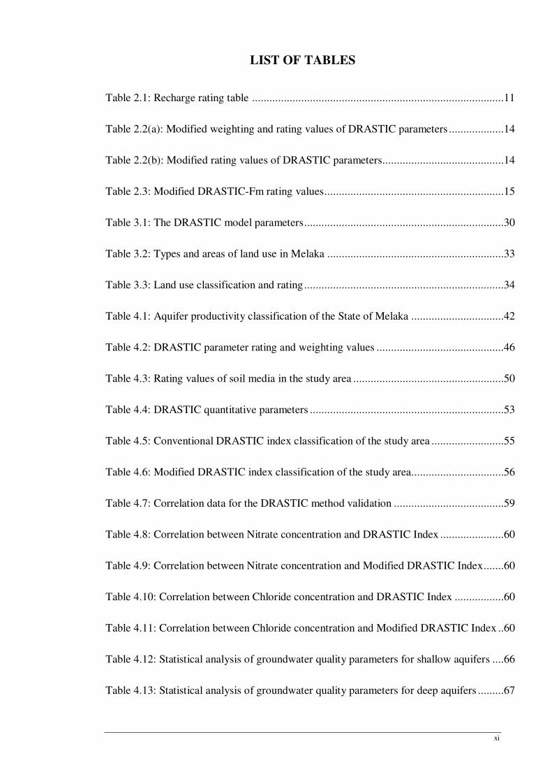
LIST OF TABLES
Table 2.1: Recharge rating table .......................................................................................11
Table 2.2(a): Modified weighting and rating values of DRASTIC parameters ...................14
Table 2.2(b): Modified rating values of DRASTIC parameters ..........................................14
Table 2.3: Modified DRASTIC-Fm rating values ..............................................................15
Table 3.1: The DRASTIC model parameters .....................................................................30
Table 3.2: Types and areas of land use in Melaka .............................................................33
Table 3.3: Land use classification and rating .....................................................................34
Table 4.1: Aquifer productivity classification of the State of Melaka ................................42
Table 4.2: DRASTIC parameter rating and weighting values ............................................46
Table 4.3: Rating values of soil media in the study area ....................................................50
Table 4.4: DRASTIC quantitative parameters ...................................................................53
Table 4.5: Conventional DRASTIC index classification of the study area .........................55
Table 4.6: Modified DRASTIC index classification of the study area ................................56
Table 4.7: Correlation data for the DRASTIC method validation ......................................59
Table 4.8: Correlation between Nitrate concentration and DRASTIC Index ......................60
Table 4.9: Correlation between Nitrate concentration and Modified DRASTIC Index .......60
Table 4.10: Correlation between Chloride concentration and DRASTIC Index .................60
Table 4.11: Correlation between Chloride concentration and Modified DRASTIC Index ..60
Table 4.12: Statistical analysis of groundwater quality parameters for shallow aquifers ....66
Table 4.13: Statistical analysis of groundwater quality parameters for deep aquifers .........67

xii
NOTATIONS
Notation Meaning
Ar Assigned ranges for critical parameter
AVI Aquifer Vulnerability Index
AWHC Available water holding capacity
CN Curve number
Cp Critical parameter
Db Diameter of basin
Dc Discontinuity ranges
DEM Digital Elevation Model
DI DRASTIC Index
DISCO DIScontinuities and protective COver parameter
Ep Evaporation
EPIK Epikarst, E; Protective cover, P; Infiltration conditions, I; and
Karst network development, K
Erate Elution rate
F Protection index
Fint Intermediate protection factor
F FD− Rate of the average of the distance from the faults system (F) and
the distance from the intersection locations between the faults
and the drainage systems (FD)
Fm Fracture Media
Fert Fertilizer input
GIS Geographic Information System
GOD Groundwater occurrence, G; Overall lithology of aquifer, O; and
Depth of groundwater level, D

xiii
Gv Groundwater vulnerability
H Length of the well screen, namely the saturated thickness of the
aquifer for full penetrating wells.
Ia Initial abstraction
Ir Weighted harmonic mean of vadose zone
Iri Rating of layer i of vadose zone
L Contaminant loading per land use category
Lr & Lw Land use rating and weighting
LU Land use
MAD Management allowable depletion (dimensionless)
n Porosity
N and N’ The number of data layers used to compute the V and V'
Nn Net recharge
Ncon Nitrate concentration in percolation water
Nw and Nr Weight and rating that given the total on-ground nitrogen loading
Pa Percentage of the total area covered by each land-use category
Pc Cumulative amount of rainfall
PI Percolation index
Pp Annual average rainfall/Precipitation
Pr and Pw Weight and rating of individual DRASTIC parameters that used
for effective weight calculation
Pt Protective cover ranges
Q Actual runoff
Qp Pumping rate of the well
r Rating of the parameters
Rc Radius of the circle

xiv
Rr Recharge rate
RF Rainfall factor
RPR Runoff potential ratio
RV Recharge value
SEEPAGE System for Early Evaluation of Pollution Potential of Agricultural
Groundwater Environments
Ssw Maximum watershed storage
SI Susceptibility index
SP Soil permeability
Sp Slope percentage
Sv Sensitivity analysis
Sw Volumes of storage water
Td Applied transformations to a data series
Tq Cumulative direct runoff
Tv Total thickness of the vadose zone
t Travel time for which volume was being calculated
Ti Thickness of the layer i
Vp Overall vulnerability index of a polygon.
V and V' Unperturbed and perturbed vulnerability indices
V(specific) Specific vulnerability
Vi Vulnerability index
Vintrinsic Intrinsic vulnerability
Vvxi Variation index omitting a parameter X (D, R, A, S, T, I or C)
Vxi Vulnerability index calculated without a parameter, X (D, R, A,
S, T, I, C)
w Weighting of the parameters

xv
We Effective weight
Wperc Percolation water
Xri and Xwi Range and weight for each parameter X
Z Root zone depth
α, β and γ Weighting coefficients of EPIK parameters

xvi
LIST OF APPENDICES
Appendix -A : List of publications…………………………………………..………81
Appendix - B: Aquifer distribution and geology map of Melaka…………….……..82
Appendix - C: Boreholes data of deep aquifers………………………………….….87
Appendix - D: Boreholes data of shallow aquifers……………………………….….93
Appendix - E: Drinking water quality standard – Malaysia, 1992…….………..…101
Appendix - F: Shallow and deep boreholes profile in Melaka………...…………...102
Appendix - G: Groundwater quality data in Melaka……………………….…….....112

CHAPTER 1 INTRODUCTION
1
Chapter 1
INTRODUCTION
1.1 General
Groundwater is the basic need for all human, animals and plants, particularly in the
region where other sources of water are lacking. Groundwater protection has become a
foremost concern since late 70's for public attention (U.S. Environmental Protection
Agency, 1990). Industrial wastes and chemicals also led to frequent pollution
problem. Some of those chemicals are penetrated into groundwater system and
causes contamination (Bedient et al., 1999). Very often groundwater is subjected to
severe anthropogenic activities which lead it to vulnerable. Groundwater vulnerability
refers to intrinsic characteristics that determine the sensitivity of the water to be
adversely affected by an imposed contaminant load. Intrinsic vulnerability mapping of
the groundwater is considered that some areas are more susceptible to contamination
than others (Piscopo, 2001). National Research Council (1993) define the term
"vulnerability" is the propensity or likelihood of pollutants to reach a particular position
in the groundwater system in which the pollutants preface at some location above the
uppermost aquifer. Specific vulnerability is more reliable and efficient than generic
vulnerability to contamination. Achieving the idle conditions of the specific
vulnerability is more difficult due to the adequate data sources. The term vulnerability
was used to more generalize case and reconnaissance level (Haertle, 1983; Aller et al.,
1987) and indicated as the potentiality of infiltration and dispersion of the pollutants
from the ground level into the groundwater system.
The groundwater vulnerability assessment mainly incorporates the geological and
hydro-geological settings and does not embrace pollutant attenuation. Preventive

CHAPTER 1 INTRODUCTION
2
actions are always better and cheaper than remediation and renovation of groundwater
contamination. Achieving these goals, the problem and its clarification can be predicted
with the help of groundwater vulnerability, quality and productivity assessment.
1.2 Problem Statement
The groundwater vulnerability is playing vital issue in worldwide. The anthropogenic
and agricultural activities are the most responsible for deterioration of groundwater
level and increasing vulnerability. The proper steps are urgent for water resources
development and to solve the problem of groundwater level deterioration and increasing
water demand (Nageswara & Narendra, 2006). Groundwater has major contribution in
agricultural, industrial and drinking as well as other municipal uses. Ensuring the
continuous water supply demand and mitigate adverse effect, the definite strategies and
guidelines are urgent for quality control, monitoring and management of groundwater
resource. The vulnerability assessment of groundwater is the most feasible step
regarding on these purposes.
Melaka State in Peninsular Malaysia is an important state for agricultural, industrial,
commercial and tourism aspects. It is subjected to limited groundwater resources
because of small land areas and comparatively low rainfall than other parts of Malaysia.
The most water supply systems are mainly depended on surface water or rainfall. For
the purposes of water supply, around 97% of the raw water is collected from streams or
rivers including impounding reservoirs and the remaining 3% of raw water are collected
from groundwater. The rural areas are not connected to sufficient treated drinking water
supply schemes. The clean water is supplied in some areas via sanitary wells and
gravity feed system. In this case, the house connections are not available with all water
supply schemes. The conventional treatment methods namely;- aeration, coagulation &
flocculation, sedimentation, filtration and chlorination are mostly used in major water

CHAPTER 1 INTRODUCTION
3
treatment plants of urban areas. However, only the chlorination is used in some small
water treatment plants which are not adequate. Potential water sources areas are
identified by traditionally have been known for good water quality in the rural areas. If
the water qualities of possible sources become satisfactory after test against the current
standard, then it is allowed to use for drinking and other purposes by the community.
Yet the users are also advised to boil water before consumption. Groundwater of
Melaka can be made a significant contribution in terms of increasing demand of safe
water and reduce the dependence on surface water. It also can be used as an important
source to meet the future water demand for the public supply.
The present study incorporates the concepts, significance and applicability of GIS-based
DRASTIC method for groundwater vulnerability and risk assessment. The DRASTIC is
an acronym for the seven factors considered in the method: Depth to water, net
Recharge, Aquifer media, Soil media, Topography, Impact of vadose zone, and
hydraulic Conductivity. The DRASTC method has been used to develop groundwater
vulnerability maps in many parts of the world; however, the effectiveness of the method
has shown mixed success (Rupert, 2001). DRASTIC maps are usually not calibrated to
measure contaminant concentrations (Rupert, 1999). It gives indication to the
vulnerability of groundwater to contamination regardless of the contaminant itself. In
addition, GIS technology is very helpful in facilitating data input and output processing
especially in watersheds where field data are regularly updated from frequent
monitoring and allows rapid visualization of raw data. The GIS is an efficient tool for
analyzing, interpreting and manipulating data as well as incorporating the geological,
hydrogeological and geomorphological data (Anbazhagan & Nair, 2004; Jha et al.,
2006; Jha & Peiffer, 2006). Moreover, this study also enforces the groundwater
productivity and quality in the study area as well as emphasized on the validation
system of the DRASTIC method.

CHAPTER 1 INTRODUCTION
4
1.3 Research Objectives
[a] To investigate the geological, hydrogeological, lithological and meteorological
settings as well as land use conditions of the study area.
[b] To assess the groundwater productivity and potentiality of the study area.
[c] To assess the groundwater vulnerability of the State of Melaka in Peninsular
Malaysia using the DRASTIC method and GIS techniques.
[d] To develop the modified DRASTIC method based on additional land use
parameter combining with conventional DRASTIC method.
[e] To assess the groundwater quality of the study area.
1.4 Outline of the Thesis
Chapter one is the introduction, where general background and research objectives are
provided. Chapter 2 reviews the literature on the DRASTIC method and GIS
techniques, where the original and modified DRASTIC parameters rating ranges and
weight are well described. The methodology that is used in order to complete the
research explained in chapter 3. In chapter 4, results and discussions are included. The
detail various thematic maps and results are described systematically. Chapter 5
concludes the research findings and suggests the future direction of research.

CHAPTER 2 LITERATURE REVIEW
5
Chapter 2
LITERATURE REVIEW
2.1 General
DRASTIC is the most reliable method for groundwater vulnerability assessment.
Firstly, the term vulnerability was used by a French hydrogeologist J. Margat in the late
60's in hydrogeology. After that it has been widely used in different parts of the world
since the last 1980's (Haertle, 1983; Aller, et al., 1987; Foster & Hirata, 1988). Under
this chapter, some previous research methodologies and outcomes were discussed on
the DRASTIC model and groundwater quality. Most of the cases, Remote Sensing
(RS), GIS, geological, hydrogeological, topographical, lithological, land use and
meteorological data were used. In some cases and regions, the researchers modified or
added or remove one or more parameters from conventional DRASTIC method and
proposed the new rating and weight range values. Sensitivity analysis enriched the
DRASTIC method’s accuracy and indicated the individual impotency of each
parameter. Anthropogenic impacts added to groundwater vulnerability and quality
assessment which had a significant effect on groundwater contamination. The concepts,
significance and applicability of GIS also described through the DRASTIC method for
groundwater vulnerability assessment.
2.2 Conventional DRASTIC Method
The DRASTIC method generally used seven hydrogeological parameters to assess
groundwater vulnerability. The parameters were considered as depth to groundwater
table (D), net recharge (R), aquifer media (A), soil media (S), topography (T), impact of
vadose zone (I) and hydraulic conductivity (C). The input information such as borehole

CHAPTER 2 LITERATURE REVIEW
6
data, meteorological data, hydrological data, geology data, soil data, lithology data,
contour map, topography map were used to develop the GIS database. The method was
used considering various circumstances such as arid or semi-arid regions, agricultural,
industrial, municipal, coastal, septic tank and landfill areas. The parameters were rated
and weighted due to their relative importance to contamination. Weighting and rating
ranges were considered from 1 to 5 and 1 to 10, respectively. A multiplier defined as
weight was multiplied with each parameter rating for each interval and then the
products were summed up to calculate the final DRASTIC index. This index indicated
the relative degree of groundwater vulnerability of an area. Higher the index value
indicated the greater possibility to contamination. Final vulnerability map was
generated by integrating all the thematic maps of DRASTIC parameters through the
GIS environment.
ArcGIS software was a powerful tool to generate different thematic maps, GIS
database, format conversion, overlaying maps, integrating maps and so on. Some
extension tools (Spatial analyst, 3D analyst and Geostatistical analyst) of GIS software
are extensively used in the DRASTIC method. Many researchers and scientists assessed
groundwater vulnerability using the Equation 2.1 based on the above concept (Kim &
Hamm, 1999; Ibe et al., 2001; Withowski et al., 2003; Tovar & Rodriguez, 2004; De
Silva & Hohne, 2005; Jasrotia & Singh, 2005; Shahid & Hazarika, 2007; Chitsazan &
Akhtari, 2009; Moghaddam et al., 2010).
DRASTIC Index (DI) Tr w r w r w r w r w r w r w
D D R R A A S S T I I C C= + + + + + + ..................... (2.1)
Where, w = weight of the parameters and r = ratings of the parameters. Groundwater
vulnerability assessment in the coastal region was an important issue. The colluvial-
alluvial sediment region was more vulnerable to contamination (Junior Silva & Pizani,
2003). The input data sources were used as groundwater depth, aquifer recharge,
lithology, soil types, topography and permeability. Anthropogenic activities and sea

CHAPTER 2 LITERATURE REVIEW
7
water intrusion were prevailing factor for groundwater vulnerability. Conventional
DRASTIC method was used in the arid region of Barka region of Oman (Jamrah et al.,
2008). The study showed the long-term changes of vulnerability index for 1995 and
2004. Groundwater samples were analyzed for major ions, nutrients, COD (Chemical
Oxygen Demand), BOD (Biochemical Oxygen Demand) and bacteria to cross check the
DRASTIC vulnerability index. Major anions such as No3-, No2
-, Cl-, So42-, Po4
2-, F-, and
Br- were analyzed to develop the correlations with vulnerability index values for
checking the DRASTIC method accuracy.
2.3 Sensitivity Analysis of the DRASTIC Parameters
Sensitivity analysis was carried out to show the relationship between the effective and
theoretical weight of the DRASTIC parameters. The analysis helped to avoid the
subjectivity to nature for vulnerability assessment which provided very important
information to assign the weighting and rating ranges of the parameters. Generally, map
removal sensitivity and single parameter removal sensitivity analysis were carried out to
indicate the most sensitive parameter for groundwater vulnerability. First one
represented the sensitivity of the final vulnerability map by removing one or more map
layers and worked out Equation (2.2). The single parameter removal sensitivity analysis
test indicated the influence of each parameter on final vulnerability measurement.
Effective weight of each subarea was estimated by the Equation (2.3). From the
sensitivity analyzed results, researchers can be understood that their assign weight was
perfect or need to modification. Both the conventional DRASTIC method and
sensitivity analysis were used to groundwater vulnerability assessment by many
researchers and scientists (Kwansiririkull et al., 2004; Babiker et al., 2005; El-Naqa et
al., 2006; Ckakraborty et al., 2007; Bazimenyera & Zhonghua, 2008; Rahman, 2008;
Hasiniaina et al., 2010; Al Hallaq & Elaish, 2011; Samake et al., 2011).
CHAPTER 2 LITERATURE REVIEW
8
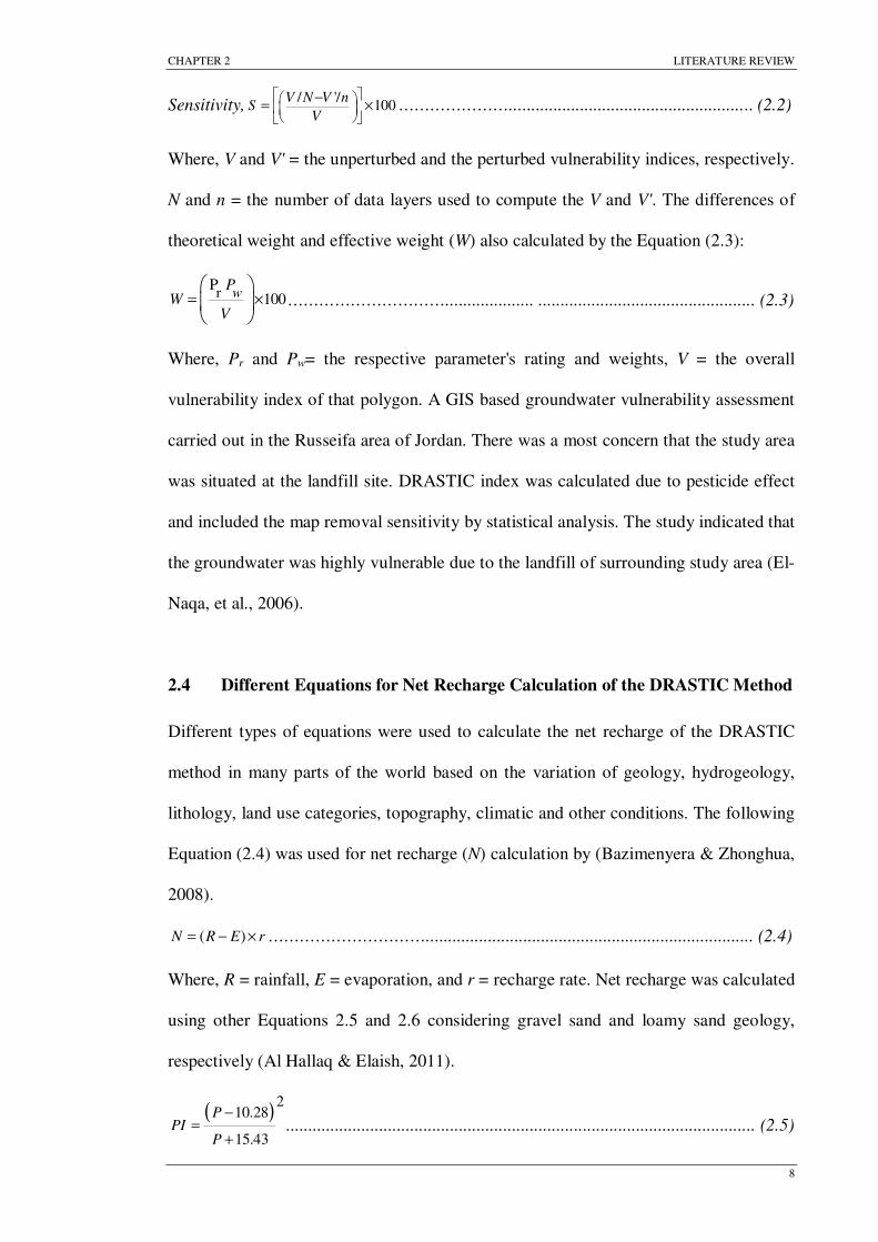
Sensitivity,/ '/
100V N V n
SV
−= × …………………....................................................... (2.2)
Where, V and V' = the unperturbed and the perturbed vulnerability indices, respectively.
N and n = the number of data layers used to compute the V and V'. The differences of
theoretical weight and effective weight (W) also calculated by the Equation (2.3):
rP
100wP
WV
= ×
………………………….................... ................................................. (2.3)
Where, Pr and Pw= the respective parameter's rating and weights, V = the overall
vulnerability index of that polygon. A GIS based groundwater vulnerability assessment
carried out in the Russeifa area of Jordan. There was a most concern that the study area
was situated at the landfill site. DRASTIC index was calculated due to pesticide effect
and included the map removal sensitivity by statistical analysis. The study indicated that
the groundwater was highly vulnerable due to the landfill of surrounding study area (El-
Naqa, et al., 2006).
2.4 Different Equations for Net Recharge Calculation of the DRASTIC Method
Different types of equations were used to calculate the net recharge of the DRASTIC
method in many parts of the world based on the variation of geology, hydrogeology,
lithology, land use categories, topography, climatic and other conditions. The following
Equation (2.4) was used for net recharge (N) calculation by (Bazimenyera & Zhonghua,
2008).
( )N R E r= − × ………………………….......................................................................... (2.4)
Where, R = rainfall, E = evaporation, and r = recharge rate. Net recharge was calculated
using other Equations 2.5 and 2.6 considering gravel sand and loamy sand geology,
respectively (Al Hallaq & Elaish, 2011).
( )2
10.28
15.43
PPI
P
−=
+.......................................................................................................... (2.5)

CHAPTER 2 LITERATURE REVIEW
9
( )2
15.05
22.57
PPI
P
−=
+.......................................................................................................... (2.6)
Where, PI = the percolation index and P = the annual average rainfall. Jayasekera et al.
(2011) estimated the recharge value by sum up the rainfall and irrigation return flow,
and subtracting the evapotranspiration. Soil moisture content was accounted to calculate
the irrigation return flow. The volume of storage water available for plants (S) was
calculated using Equation (2.7):
2
4 100
D AWHCbS MAD Z
π= × × × ....................................................................................... (2.7)
Where, Db = diameter of basin, Z = root zone depth; AWHC = available water holding
capacity, MAD = management allowable depletion (dimensionless). The assumptions
were Z = 0.5 m; AWHC = 8% and MAD = 1.0 for desert plants and 0.5 for others plants.
It was used the approximate infiltration fraction as 0.4 based on rainfall
(Kuruppuarachchi, 1995). The calculated fraction of irrigation water recharge to
groundwater table was 0.63 over the area. Fault system, fault density, the distance
between fault system intersection and drainage system intersection, rainfall amount,
slope of the area and soil permeability were greatly considered (Al-Hanbali & Kondoh,
2008) to estimate the net recharge using Equation (2.8).
RV RF S SP F FD= + + + − ………………………………….............…….......................... (2.8)
Where, RV = recharge value, RF = rainfall factor, F FD− = the rate of the average of
the distance from the faults system (F) and the distance from the intersection locations
between the faults and the drainage systems (FD). S = slope percentage, SP = soil
permeability. A study was carried out by greatly considered the net recharge calculation
method and its rating system by (Kim & Hamm, 1999). In this case, Soil Conservation
Service (SCS) method was used (Morel-Seytoux & Verdin, 1981) to define the net
recharge rate. Cumulative direct runoff (Tq) was calculated by the Equations (2.9 to
2.11):

CHAPTER 2 LITERATURE REVIEW
10
( )2
aq
a
P IT
P I S
−=
− +…………………………………………………....................................... (2.9)
, 0.2a
Again I S= ……………………………………………………..…............................ (2.10)
25400254S
CN= − ……………………………………………………...................................
(2.11)
Where, P = cumulative amount of rainfall, Ia = initial abstraction, S = maximum
watershed storage and CN = curve number. CN value was depended on the watershed
soil types and land use categories. The soil was classified according to SCS
classifications and land use was classified according to US geological survey. Under
SCS method, runoff potential was determined based on Antecedent Moisture
Conditions (AMC). CN and Sp values were taken with respect to AMC classification
which taken from SCS chart. Finally, cumulative direct runoff (Tq) was calculated for
each land-use category using the Equation (2.12):
( )2
0.2
0.8q
P ST
P S
−=
+…………………………………………......………................................ (2.12)
The net recharge rating ranges (Table 2.1) were developed based on Runoff Potential
Ratio (RPR) which calculated on each land use category and by the following Equation
(2.13):
qT
RPRP
= …………………………………………………....………………......................
(2.13)
To evaluate the relative weight of RPR value, the actual runoff (Q) was calculated using
Equation (2.14):
100
aq
PQ T= × ……………………………………………......………………........................ (2.14)

CHAPTER 2 LITERATURE REVIEW
11
Where, Pa = the percentage of the total area covered by each land-use category. The
new rating ranges of net recharge were selected based on (RPR), whereas RPR mainly
depended on land use categories. The study showed that shallow aquifers were more
vulnerable due to higher recharge, hydraulic conductivity and coarse soil. The domestic
and industrial waste water were the main sources of pollution.
Table 2.1: Recharge rating table (Kim & Hamm, 1999)
RPR (%) Runoff Land use Rating
0–15 Low Forest and agricultural land 5
15–25 Moderate Barren land and alluvium 4
25–30 High Residential area and channel deposit 2
130 Very high Water 1
A recession curve displacement method was used to estimate the net recharge. Stream
flow data within the study area were used for recession curve displacement method
(Fritch, et al., 2000) and suggested the three concepts for vadose zone rating ranges. (i)
If overlaying material's thickness of the aquifer was less or equal to the thickness of
weathered zone, then vadose zone media was considered as materials of the aquifer
media. (ii) If overlaying material's thickness of aquifer was greater than the weathered
zone, but less or equal to vadose zone , then the vadose zone could be adequately
described as a weighted average: [(the aquifer material media rating × its thickness) +
(the overlying material media rating × its thickness)]/total thickness of the vadose zone.
(iii) If overlaying material thickness of the aquifer was greater than the weathered zone
and vadose zone, then vadose zone should be rated according to the overlaying
materials characteristics.

CHAPTER 2 LITERATURE REVIEW
12
2.5 Modified DRASTIC Approach
Land use had a potential impact on groundwater vulnerability and risk mapping which
were produced as consequence of groundwater contamination. Modified DRASTIC
method was used to assess the groundwater vulnerability and risk mapping including
land use (Secunda et al., 1998; Al-Adamat, et al., 2003), and considered D, R, A, S, T
and I parameters because of lacking the hydraulic conductivity data. The fixed value 68
assumed instead of (DrDw + ArAw + IrIw) index value. Since the possible minimum and
maximum DRASTIC index was 24 and 220 and divided into four vulnerability classes
(i) 24–71 (No risk), (ii) 72–121 (Low), (iii) 122–170 (Moderate) and (iv) 171–220
(High). Final modified DRASTIC index (MDi) was calculated using the following
Equation (2.15):
( )i r wMD DI L L= + …………………………………………....……………........................ (2.15)
Where, DI = the DRASTIC index. Lr and Lw = the land use rate and weight,
respectively. Khan et al. (2010) focused on the land use and impact of vadose zone
effect on groundwater vulnerability and risk assessment using DRASTIC method. Land
use weight was considered as 5 and hydraulic mean approach (Hussain et al., 2005) was
used to calculate the impact of vadose zone parameter. The following Equation (2.16)
was used to achieve the approach and final vulnerability index calculated using the
Equation (2.1):
1
ri
ri
TI
Tn
i I
=
∑=
............................................................................................................. (2.16)
Where, Ir= the weighted harmonic mean of the vadose zone, T = the total thickness of
the vadose zone, Ti= thickness of the layer I, and Iri= the rating of the layer i. Al-
Hanbali & Kondoh (2008) also used the Equation (2.1) to assess groundwater
vulnerability. Modified DRASTIC parameters and rating ranges were used in most
cases of arid and semi-arid regions. Weight and rating ranges were changed due to
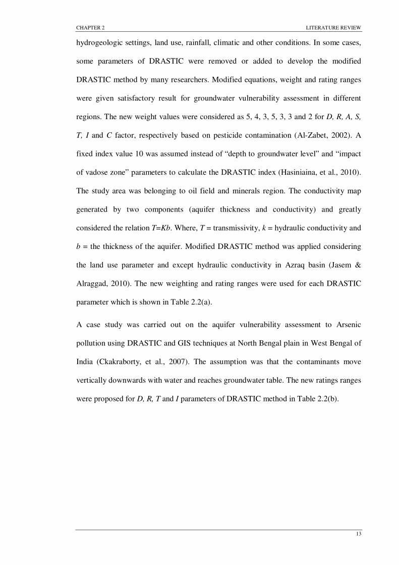
CHAPTER 2 LITERATURE REVIEW
13
hydrogeologic settings, land use, rainfall, climatic and other conditions. In some cases,
some parameters of DRASTIC were removed or added to develop the modified
DRASTIC method by many researchers. Modified equations, weight and rating ranges
were given satisfactory result for groundwater vulnerability assessment in different
regions. The new weight values were considered as 5, 4, 3, 5, 3, 3 and 2 for D, R, A, S,
T, I and C factor, respectively based on pesticide contamination (Al-Zabet, 2002). A
fixed index value 10 was assumed instead of “depth to groundwater level” and “impact
of vadose zone” parameters to calculate the DRASTIC index (Hasiniaina, et al., 2010).
The study area was belonging to oil field and minerals region. The conductivity map
generated by two components (aquifer thickness and conductivity) and greatly
considered the relation T=Kb. Where, T = transmissivity, k = hydraulic conductivity and
b = the thickness of the aquifer. Modified DRASTIC method was applied considering
the land use parameter and except hydraulic conductivity in Azraq basin (Jasem &
Alraggad, 2010). The new weighting and rating ranges were used for each DRASTIC
parameter which is shown in Table 2.2(a).
A case study was carried out on the aquifer vulnerability assessment to Arsenic
pollution using DRASTIC and GIS techniques at North Bengal plain in West Bengal of
India (Ckakraborty, et al., 2007). The assumption was that the contaminants move
vertically downwards with water and reaches groundwater table. The new ratings ranges
were proposed for D, R, T and I parameters of DRASTIC method in Table 2.2(b).

CHAPTER 2 LITERATURE REVIEW
14
Table 2.2(a): Modified weighting and rating values of DRASTIC parameters
Table 2.2(b): Modified rating values of DRASTIC parameters
DRASTIC-Fm (Fracture Media) method was applied to assess the groundwater
vulnerability for the structural characteristics of fractured bedrock aquifers (Denny et
al., 2007). The fractured media was strictly considered for the identifying its effect on
groundwater vulnerability. The fractured media was classified as three categories

CHAPTER 2 LITERATURE REVIEW
15
(Fracture orientation, Fracture length and Fracture density) and also the rating ranges
were assigned for those categories. The Fm factor was rated according to the rating
range in Table 2.3. The weight of Fm factor was considered as 3.
Table 2.3: Modified DRASTIC-Fm rating values
30° fault orientation classification and associated
DRASTIC-Fm ratings
Length classifications and associated
DRASTIC-Fm ratings
Fracture density classifications and associated
DRASTIC-Fm ratings
Exte
nsi
on
Minm Maxm Rating Fracture length
(m) Rating
Fracture density (fractures/m)
Rating
285 315 7 20000-25000 10 0-2 2
315 345 10 15000-20000 8 2-4 4
345 15 7 10000-15000 6 4-6 6
105 135 7 5000-10000 4 6-8 8
135 165 10 0-5000 2 >8 10
165 195 7 - - - -
Contr
acti
on 195 225 4 - - - -
225 255 2 - - - -
255 285 4 - - - -
15 45 4 - - - -
45 75 2 - - - -
75 105 4 - - - -
2.6 Calibration of the DRASTIC Method
Groundwater vulnerability was assessed in many parts of the world considering nitrate
contamination. Nitrogen is the basic need for agricultural plants to ensure the high
production (Lake et al., 2003; Schröder et al., 2004; Shirazi et al., 2011). Groundwater
greatly affected by the nitrate contamination all over the world (Birkinshaw & Ewen,
2000; Saâdi & Maslouhi, 2003; Kyllmar et al., 2005; Liu et al., 2005). Nitrate
contamination mainly occurred in the agricultural areas due to application of fertilizers.
The soil compositions (soil leaching potential) have a great effect on Decision Support
System to minimize the pollution of groundwater from agrochemicals (Brown et al.,
2003; Holman et al., 2004). The nitrate concentration in groundwater depends on soil
nitrate levels, and the timing and amount of surface loading (Di & Cameron, 2002). One
of the non-point source pollution of groundwater is caused by nitrate in the agricultural

CHAPTER 2 LITERATURE REVIEW
16
areas (Hubbard & Sheridan, 1994; Mclay et al., 2001; Shamrukh et al., 2001; Harter et
al., 2002; Almasri & Kaluarachchi, 2004; Chowdary et al., 2005). On-ground nitrogen
concentration was considered to assess the groundwater vulnerability. Nitrogen
database was very effective to validate the intrinsic vulnerability (Holman et al., 2005).
The on-ground nitrogen loading was rated and weighted, and then added with
DRASTIC index. Finally, the composite DRASTIC index (CDI) was calculated by the
following Equation (2.17):
w rCDI DI N N= + ....................................................................................................... (2.17)
Where, DI = the conventional DRASTIC index, Nw and Nr= the weight and rating that
given the total on-ground nitrogen loading. The intrinsic vulnerability was assessed to
nitrate contamination and considered five parameters for the modification of the
DRASTIC method (Mishima et al., 2011). Only vertical movement of contamination
was considered for this modification. In this case, the aquifers were shallow and aquifer
media was in narrow range. Soil media was governed by the aquifer media parameter.
Hydraulic conductivity and aquifer media were less effective for contamination. The
more recharge value was considered as less rating value and less recharge value was
considered as high rating value which was opposite of original DRASTIC and the
Equation (2.18) was used to calculate the nitrate concentration:
rate ertcon
perc
E FN
W
×= ..................................................................................................... (2.18)
Where, Ncon = nitrate concentration in percolation water (mg/L), Erate = elution rate, Fert
= fertilizer input (kg/ha), Wperc = percolation water (mm/year). Finally, Modified
DRASTIC index was calculated by Equation (2.19):
v r w r w r w r w r wG D D R R S S T T I I= + + + + ...................................................................... (2.19)
Where, Gv = groundwater vulnerability, r and w = rating and weighting of the
parameters. The new weighting and rating ranges were proposed for five parameters of

CHAPTER 2 LITERATURE REVIEW
17
DRASTIC based on agricultural areas (Javadi et al., 2011). The new rating ranges are
shown in Table 2.2(b).
DRASTIC method was improved by calibrating the point rating scheme, which
measured nitrate (NO3) & nitrite (NO2) concentration in groundwater (Rupert, 1999).
Statistical correlations were developed between the land use, soil, depth to groundwater
level and nitrate & nitrite concentrations. GIS and statistical techniques were applied to
enumerate the correlations. Based on the correlations the probability map of nitrate &
nitrite were generated. Then conventional DRASTIC map and probability map were
compared with the independent set of nitrate & nitrite data. The comparison showed
that poor correlations were found between the conventional DRASTIC map and nitrate
& nitrite concentrations. There was no significance difference of nitrate & nitrite
concentration in groundwater between the low, medium, high and very high
vulnerability category areas. Good correlations were found between the probability map
and nitrate & nitrite concentration. The significant difference of nitrate & nitrite
concentration in groundwater indicated between the low, medium, high and very high
vulnerability category areas. The study suggested that groundwater vulnerability and
probability maps can be used to develop the prevention guidelines for high susceptible
to contamination areas. Groundwater vulnerability was assessed considering the severe
human impact, semi-arid climate and very little slope variation (Chitsazan & Akhtari,
2009). The most aquifer systems of the study area were unconfined. DRASTIC method
was evaluated by the nitrate concentration value of the study area. The correlations were
shown between the DRASTIC parameters and nitrate concentration value using the
multivariate statistical method.

CHAPTER 2 LITERATURE REVIEW
18
2.7 Comparison of the DRASTIC with Other Methods
A regional scale of groundwater vulnerability assessment was carried out based on
nitrate contamination using the conventional DRARTIC and SEEPAGE (System for
Early Evaluation of Pollution Potential of Agricultural Groundwater Environments)
method (Navulur, 1996). The vulnerability map showed that 24% area was high
vulnerability and 28% very high vulnerability according to the assessment of DRASTIC
and SEEPAGE method, respectively. The Bayesian probability map also developed for
both methods for computing the probabilities of nitrate occurrence. The probability
maps showed that 26% and 21% area with a probability of nitrate recognition > 50%
using DRASTIC and SEEPAGE factors, respectively. The water quality data indicated
that 76% of the nitrate recognitions were within the areas with probability of
recognition > 50%. The study suggested that statistical techniques can be used to
generate the regional scale risk map where data availability is limited and DRASTIC
performance is better than SEEPAGE.
DRASTIC and AVI (Aquifer Vulnerability Index) methods were used to assess
groundwater vulnerability mapping and checked the validation of DRASTIC method
(Leal & Castillo, 2003). To validate the weighting and rating ranges of the parameters,
the raw data maps and parameter rating maps were compared. Overlaying isoline map
pair’s technique was used to compare between different maps. If major variations were
detected then the rating ranges were modified. Depth to groundwater table parameter
was adjusted and proposed for rescaling the rating ranges. The simplification was
represented by the matrix form as Equation (2.20):
= d r pT A C ....................................................................................................... (2.20)
Where, Ar = geological maps, well log data, pump test data. Td = the applied
transformations to a data series, and Cp = critical parameters. Again, critical parameter
Cp affected by the weight function W and it presented by Equation (2.21).

CHAPTER 2 LITERATURE REVIEW
19
[ ] [ ]= p
W C Vi ………………………………………….........……………….................... (2.21)
Where, W = the assigned weight, and Vi= the vulnerability index. Effective weight (We)
was calculated (Napolitano & Fabbri, 1996; Gogu & Dasargues, 2000) based on the
Equation (2.22).
100×
= ×ri wie
i
X XW
V................................................................................................... (2.22)
Where, Xri and Xwi= the ranges and weight for each parameter X, and Vi= the
vulnerability index. The vulnerability variation was calculated (Lodwik et al., 1990)
based on Equation (2.23) and proposed new rating for depth to groundwater table
parameter.
( )100
i xivxi
i
V VV
V
−= × ................................................................................................... (2.23)
Where, Vvxi = variation index omitting a parameter X (D, R, A, S, T, I or C), Vi =
vulnerability index in the point i, and Vxi = vulnerability index calculated without a
parameter, X (D, R, A, S, T, I, C). The comparison between different vulnerability
assessment method such as AVI, GOD (Groundwater occurrence, G; Overall lithology
of aquifer, O; and Depth to groundwater level, D), DRASTIC and EPIK (Epikarst, E;
Protective cover, P; Infiltration conditions, I; and Karst network development, K) were
conducted for diffuse flow carbonate aquifers (Vias et al., 2004). The aquifer was high
vulnerable according to the AVI method and moderate vulnerable according to the other
three methods. The vulnerability maps indicated that AVI method was not suitable
whereas GOD method was adequate for vulnerability assessment of diffuse flow
carbonate aquifers. Lithological parameters were the most significant for groundwater
pollution potential while depth to groundwater level had minor influence. High
vulnerability area was resulting by EPIK method for the fractured zones which
contradicted with very low karst areas. Among above methods, EPIK is adequate for
CHAPTER 2 LITERATURE REVIEW
20
karstification areas and GOD is adequate for poor karstification carbonate areas.
Moreover, DRASTIC and AVI methods are more suitable for land use management.
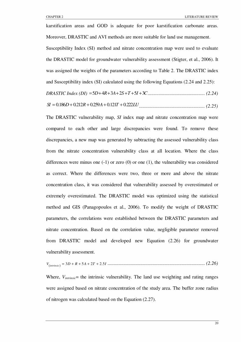
Susceptibility Index (SI) method and nitrate concentration map were used to evaluate
the DRASTIC model for groundwater vulnerability assessment (Stigter, et al., 2006). It
was assigned the weights of the parameters according to Table 2. The DRASTIC index
and Susceptibility index (SI) calculated using the following Equations (2.24 and 2.25):
DRASTIC Index (DI) 5 4 3 2 5 3D R A S T I C= + + + + + + ............................................... (2.24)
0.186 0.212 0.259 0.121 0.222= + + + +SI D R A T LU...................................................... (2.25)
The DRASTIC vulnerability map, SI index map and nitrate concentration map were
compared to each other and large discrepancies were found. To remove these
discrepancies, a new map was generated by subtracting the assessed vulnerability class
from the nitrate concentration vulnerability class at all location. Where the class
differences were minus one (-1) or zero (0) or one (1), the vulnerability was considered
as correct. Where the differences were two, three or more and above the nitrate
concentration class, it was considered that vulnerability assessed by overestimated or
extremely overestimated. The DRASTIC model was optimized using the statistical
method and GIS (Panagopoulos et al., 2006). To modify the weight of DRASTIC
parameters, the correlations were established between the DRASTIC parameters and
nitrate concentration. Based on the correlation value, negligible parameter removed
from DRASTIC model and developed new Equation (2.26) for groundwater
vulnerability assessment.
( ) 3 5 2 2.5intrinsic
V D R A T I= + + + + ................................................................................ (2.26)
Where, Vintrinsic= the intrinsic vulnerability. The land use weighting and rating ranges
were assigned based on nitrate concentration of the study area. The buffer zone radius
of nitrogen was calculated based on the Equation (2.27).

CHAPTER 2 LITERATURE REVIEW
21
π
⋅=
⋅ ⋅
p
c
Q tR
n H............................................................................................................ (2.27)
Where, Rc = the radius of the circle, Qp = the pumping rate of the well, t = the travel
time for which volume was being calculated, n = the porosity and H = the length of the
well screen. Finally, specific vulnerability of groundwater was calculated considering
land use parameter and by the Equation (2.28):
Aquifer Pollution Risk, ( )
3 5 2 2.5 5V D R A T I Lspecific
= + + + + + .................................. (2.28)
Where, L = the contaminant loading per land use category. EPIK and DRASTIC model
were used to assess the groundwater vulnerability and indicated the protection zone
(Hammouri & El-Naqa, 2008). The EPIK was a multi-attribute method which was
mainly used in karst region. The factor E and K were determined with respect to
geological and morphological information, whereas the P and I factor were determined
from soil and land use maps. The final protection index F was calculated by the
Equation (2.29):
F E p I Kα β γ δ= + + + ................................................................................................. (2.29)
Where, E = development of the Epikarst, P = effectiveness of the protective covers, I =
infiltration condition, K = development of the Karst network. Again α, β, γ and δ =
weighting coefficients. The DRASTIC model is a straightforward method and generally
it is applicable where the hydrological data are available. EPIK is used the region which
is subjected to karst features (holes, caves, sinkholes).
Groundwater vulnerability based approach was used to delineate the groundwater
protection zones around springs of fracture media (Pochon et al., 2008). Non-
consolidated porous media were used as protective materials. Considering the
hydrological diversity, individual solution was applied for each hydrological setting.
Distance method and isochrone protection method were applied for low vulnerability
and slightly vulnerability springs which consist of three protection zones such as S1, S2

CHAPTER 2 LITERATURE REVIEW
22
and S3. Zone S1 suggested that the distance must extended at least 10 m around or
upstream of the springs which integrated drains, draining trenches and galleries. Zone
S2 suggested the outer distance of S1 and S2 zones must at least 100m and zone S3
suggested that the distance between the external limits of S2 and S3 zones equal to the
same distance between the outer limits of S1 and S2 zones. DISCO (DIScontinuities
parameter, protective COver parameter) method was applied for highly vulnerable
springs which include characterization of hydrogeological properties of the fractured
aquifer and evaluation of the thickness and permeability of protective cover. The
method was applied at four stages. Firstly, the discontinuities and protective cover
parameters maps were prepared for whole catchment area and rated the value of 'D'
(range 0-3) and 'P' (range 0-4) based on hand drilling, on-site soil analysis, geo-
morphological map, geophysics and infiltration test. Secondly, intermediate protection
factor (Fint) was calculated by the Equation (2.30):
2int
= +D Pc t
F ............................................................................................................. (2.30)
Where, Dc = discontinuity range, and Pt = protective cover range. Then intermediate
protection map was prepared. Thirdly, final protection map was modified by updating
the intermediate protection map based on runoff parameter, slope gradient and soil
permeability. Fourthly, protection map was converted into protection zones using some
conversion factor. The discontinuity and protective cover factors were considered to
generate the discontinuity map and protection zone map for the study area. In
conclusion, the effectiveness of the study needs to verify from data of long term
groundwater quality monitoring and further case studies.
2.8 Overview of the DRASTIC Method
Groundwater vulnerability is a widespread problem in worldwide. Two main
components are considered for the DRASTIC method;- (i) the map able units which are

CHAPTER 2 LITERATURE REVIEW
23
called hydrogeologic settings, and (ii) the application of numerical values of the relative
ranking of the hydrogeologic factors. This chapter attempts to present the application of
the DRASTIC method for groundwater vulnerability assessment, moreover some
comparison between the DRASTIC and other related methods are presented. The GIS
techniques are provided the great facilities to accomplish and handle the complex and
extensive databases for groundwater vulnerability assessment. The salient literature
overviews are summarized below:
[a] The modified DRASTIC method is better than conventional DRASTIC method
in the arid, semi-arid, basaltic, and agricultural and land fill regions.
[b] Sensitivity analysis is very helpful for DRASTIC method. It indicates which
parameter has the most significant contribution to groundwater vulnerability.
The differences between theoretical and effective weights of DRASTIC
parameters are demonstrated by sensitivity analysis.
[c] Extensive approaches are established to net recharge calculation based on
different geological and hydrogeological conditions.
[d] The DRASTIC method is calibrated by nitrate concentration in groundwater or
others related method. The evaluation system is the comparison between
vulnerability index maps of various methods or correlation between the
vulnerability index values and nitrate concentration values over the study area.
[e] In some cases, the DRASTIC parameter's weighting and rating ranges can be
modified and one or more parameters also can be added or subtracted from
conventional DRASTIC method based on the geology, hydrogeology, land use
categories, climatic and others conditions.
[f] In agricultural areas, it is better to rescale the weighting and rating ranges of
conventional DRASTIC parameters due to land use and nitrate concentration
resulting from pesticides and fertilizers.

CHAPTER 3 METHODOLOGY
24
Chapter 3
METHODOLOGY
3.1 General
The chapter describes the approach and the development of conventional and modified
DRASTIC methods as well as drilling methodology to assess the groundwater
vulnerability, potentiality and quality of the State of Melaka in Peninsular Malaysia.
The preparation of data is discussed in detail for the development of groundwater
vulnerability and potentiality maps. The study focuses the modified DRASTIC method,
which included the land use parameter. This chapter contains of three sections, in which
first section addressing the drilling methodology, second the conventional DRASTIC
method and third the modified DRASTIC method.
3.2 Description of the Study Area
3.2.1 Location
Melaka is ranked as the third smallest state in Peninsular Malaysia with a land area of
1650 Sq. Km. The location is between latitudes 1◦06’ and 2◦30’ N and longitudes
101◦58’and 102◦35’ E (Figure 3.1). Melaka located on the southwestern coast of
Peninsular Malaysia opposite Sumatra, with the states of Negeri Sembilan to the north
and Johor to the east. The capital town of Melaka is strategically situated between the
two national capitals of Malaysia and Singapore. The State of Melaka is included three
important Districts, which are Alor Gajah, Melaka Tengah and Jasin. The Districts are
divided into 81 mukims (parishes). The population of Melaka is about 0.605 million and
the density is 385 persons per Sq. Km. (Statistics Department of Malaysia, 2000).

CHAPTER 3 METHODOLOGY
25
Figure 3.1: Melaka state of Peninsular Malaysia as study area
3.2.2 Climate
The weather of Melaka state is humid and hot through the year with heavy rainfall. The
rainfall is not uniform all over the year. It varies slightly month to month. Melaka State
is mostly wetted in September to December. Generally, it rains in the afternoon
resulting from the humid and hot temperature conditions. The ranges of temperature are
30°C - 35°C during the day, and 27°C - 29°C at night.
3.2.3 Dam and Water Plant
A dam is a barrier which impounds water or underground streams. Primary purpose of
dam is to retain water, while the other structures such as floodgates or levees are used to
manage or prevent water flow into specific land regions. Another function of dam is
used to generate electricity. Furthermore, it also uses to collect or storage water which
distributes this storage water into the various locations. The main water utility sources

CHAPTER 3 METHODOLOGY
26
of Melaka are some dams and water treatment plants. Melaka state has some important
dams and water treatment plants such as Durian Tunggal dam, Jus dam, Jerneh dam,
Cincin water plant, Merlimau water plant, Bertam water treatment plant, Gadek water
treatment plant and Asahan water treatment plant. Among these, the Durian Tunggal
and Jus dam are the main two dams in Melaka for water supply. The capacity of the
Durian Tunggal is 32,600 ML and the area of water catchment is 41.4 Km/m3 which is
8% of 505.5 Km/m3 of Melaka River water catchment. Jus is the largest dam in Melaka
and located in Jasin district. It's capacity is 45000 ML. Jas dam is filled by raw water
from the Durian Tunggal dam via Machap Pump Station with capacity of 100 ML per
day through the pipeline of 12.4 Km. About 80 to 90% water demand of Melaka is
supplied by the Melaka and Kesang River and the rest is imported from the Muar River
in Johor.
3.3 Drilling Methodology
The groundwater potentiality and quality assessment methodology include the
observation of the boreholes drilling operations in the study area. The boreholes were
drilled until reaching the fractured zones, which was the high potential for groundwater
storage. In order to understand and identify the groundwater quality and potentiality;-
geological, hydro-geological, geo-physical, test drilling, pumping test and hydro-
chemical investigations were carried out. The Melaka State Government built 238
shallow boreholes (depth < 20 m), which were distributed in the territory of Alor Gajah,
Central Melaka and Jasin, while more than 20 deep boreholes (depth > 50m) were
mostly drilled by the private sector under the supervision of Melaka territory.
The upper portion of the deep boreholes was formed by a 355 mm diameter steel casing
with a 200 mm PVC pipe casing being used in the lower parts. The drilling methods
were Rotary Drilling with Water Circulation, Air Percussion Rotary and Air-Foam

CHAPTER 3 METHODOLOGY
27
Rotary. The maximum drilling depth was around 200m. Rotary drilling with the water
circulation method was applied for the upper soft residual soil, sedimentary and
weathered bedrock. Air percussion rotary drilling was applied to drill the medium hard
and semi-weathered or unweathered bedrock for the 350 mm diameter borehole. An air
compressor was used to bring the rock chips to the ground surface generating 250 psi
pressure in which the borehole diameter was 210mm. Boreholes which were able to
meet the satisfactory discharge rate to be developed as production wells. The
development was conceded using the airlift method. The operation carried out for at
least 6 hrs or until the airlifted water became clean and sand free. The optimum yields
of the boreholes were estimated using the constant discharge rate and step drawdown
method. The rate of discharge was estimated by measuring the height of the water flow
over a 90º V-notch weir using the following Equation (3.1):
2.481.34Q H= ............................................................................................................... (3.1)
Where, Q = the rate of discharge (m3/day), and H = the vertical distance in meters from
the crest of the weir to the free water surface. The groundwater samples were collected
for quality analysis during the pumping tests. The quality analysis carried out according
to the Standard Method (APHA, 1981).
3.4 The DRASTIC Model Description
3.4.1 DRASTIC Approach
The DRASTIC vulnerability index is a linear combination of seven hydrogeological
factors. It is one of the most widely used methods to assess the intrinsic vulnerability of
groundwater to contamination (Rupert, 1999). The DRASTIC is also defined as Point
Count System Model (PCSM) or a Parameter Rating and Weighting Method. A
multiplier called weight is attributed to each DRASTIC parameter based on its relative
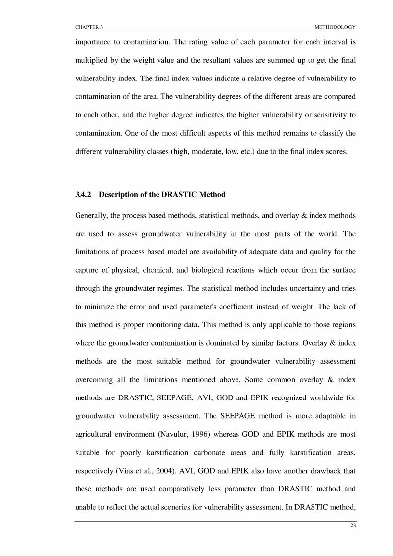
CHAPTER 3 METHODOLOGY
28
importance to contamination. The rating value of each parameter for each interval is
multiplied by the weight value and the resultant values are summed up to get the final
vulnerability index. The final index values indicate a relative degree of vulnerability to
contamination of the area. The vulnerability degrees of the different areas are compared
to each other, and the higher degree indicates the higher vulnerability or sensitivity to
contamination. One of the most difficult aspects of this method remains to classify the
different vulnerability classes (high, moderate, low, etc.) due to the final index scores.
3.4.2 Description of the DRASTIC Method
Generally, the process based methods, statistical methods, and overlay & index methods
are used to assess groundwater vulnerability in the most parts of the world. The
limitations of process based model are availability of adequate data and quality for the
capture of physical, chemical, and biological reactions which occur from the surface
through the groundwater regimes. The statistical method includes uncertainty and tries
to minimize the error and used parameter's coefficient instead of weight. The lack of
this method is proper monitoring data. This method is only applicable to those regions
where the groundwater contamination is dominated by similar factors. Overlay & index
methods are the most suitable method for groundwater vulnerability assessment
overcoming all the limitations mentioned above. Some common overlay & index
methods are DRASTIC, SEEPAGE, AVI, GOD and EPIK recognized worldwide for
groundwater vulnerability assessment. The SEEPAGE method is more adaptable in
agricultural environment (Navulur, 1996) whereas GOD and EPIK methods are most
suitable for poorly karstification carbonate areas and fully karstification areas,
respectively (Vias et al., 2004). AVI, GOD and EPIK also have another drawback that
these methods are used comparatively less parameter than DRASTIC method and
unable to reflect the actual sceneries for vulnerability assessment. In DRASTIC method,

CHAPTER 3 METHODOLOGY
29
the rating and weight values are assigned precisely according to the range and
individual categories of the each parameter in which the parameters are more
interrelated. So, if any case some data are unavailable or missing, it does not show the
great discrepancy in final vulnerability results. The DRASTIC method is based on the
assumptions that some known major factors control the groundwater vulnerability and
those can be weighted. It is very costly and time consuming to assess groundwater
vulnerability for a specific site, whereas DRASTIC method is more economic and less
time consumable to assess wide range of regional groundwater vulnerability
overcoming sloppy, uncontrolled development of land and undesirable activities. The
method was first developed by Aller et al. (1987) combined with the National Well
Association and the US Environmental Protection Agency (EPA) for evaluating the
groundwater susceptibility to contamination on a regional scale. Then the method has
been modified by many researchers and scientists based on geological or hydro-
geological settings, climate conditions and other specific situations. The most widely
used groundwater vulnerability mapping method to assess the groundwater vulnerability
for a wide range of contamination is an empirical model called DRASTIC (Evans &
Myers, 1990; Knox et al., 1993; Kim & Hamm, 1999; Fritch et al., 2000; Piscopo, 2001;
Al-Adamat et al., 2003; Thirumalaivasan et al., 2003; Murat et al., 2004; Herlinger &
Viero, 2006; Stigter et al., 2006; Rahman, 2008).
The method is being used more and more in Europe and Latin America (Leal &
Castillo, 2003; Lobo-Ferreira & Oliveira, 2003). The aim of the model is to identify the
areas, where a particular attention and more protection attempts are needed. The set of
variables are grouped into three categories; land surface factors, unsaturated zone
factors and aquifer or saturated zone factors which are the important considerations for
the DRASTIC model (Hasiniaina et al., 2010). The model has four assumptions;- (1)
The contaminants are induced at the ground surface, (2) Contaminant is flushed into the

CHAPTER 3 METHODOLOGY
30
groundwater system by precipitation, (3) The contaminant has the mobility of water,
and (4) The area being evaluated by DRASTIC is 100 acres or larger. The DRASTIC
parameters are weighted according to the assumption of Aller, et al. (1987) and
presented in Table 3.1.
In Melaka catchment, the DRASTIC method is used because the study focused on a
large region not on a specific local small field or special contaminants. Moreover, the
method is every cost effective and availability of required data.
Table 3.1: The DRASTIC model parameters
Factor Description Relative weight
Depth of water table
Represents the depth from the ground surface to the water table, deeper water table levels imply lesser chance for contamination to occur.
5
Net recharge Represents the amount of water that penetrates the ground surface and reaches the water table, recharge water represents the vehicle for transporting pollutants.
4
Aquifer media Refers to the saturated zone material properties, it controls the pollutant attenuation processes.
3
Soil media Represents the uppermost weathered portion of the unsaturated zone and controls the amount of recharge that can infiltrate downward.
2
Topography Refers to the slope of the land surface, it dictates whether the runoff will remain on the surface to allow contaminant percolation to the saturated zone
1
Impact of vadose zone
Is defined as the unsaturated zone material, it controls the passage and attenuation of the contaminated material to the saturated zone.
5
Hydraulic conductivity
Indicates the ability of the aquifer to transmit water, hence determines the rate of flow of contaminant material within the groundwater system.
3
The final vulnerability index is calculated based on the each parameter rating ranges
and its corresponding weights. The rating and weight ranges varies from 1 to 10 and 1
to 5, respectively. Each parameter is rated and weighted due to their relative importance

CHAPTER 3 METHODOLOGY
31
on groundwater contamination. The higher tendency to pollution is assigned as the
higher rating and weighting value of the respective parameter. Final DRASTIC Index is
calculated applying a linear combination of all parameters based on the following
Equation (3.2).
DRASTIC Index Tr w r w r w r w r w r w r w
D D R R A A S S T I I C C= + + + + + + .......................... (3.2)
Where D, R, A, S, T, I, and C represents the seven hydrogeological parameters and the
subscripts r and w represents the corresponding rating and weighting of the parameters,
respectively. The DRASTIC groundwater vulnerability mapping procedures are
incorporated with the help of GIS. The GIS is a computerized mapping and spatial data
analysis system, which enables to manipulation and analysis of spatially referenced
information. Though the DRASTIC method is not originally designed as a GIS-based
tool, the model lends itself for implementation (Merchant, 1994). GIS applications and
its variations in the DRASTIC method have been widely reported in the literature
(Trent, 1991; Lusch et al., 1992). The GIS is used for a number of procedures in this
study, including:- (i) converting all hardcopy map into a digital format, (ii) creating
thematic maps of DRASTIC parameters using water depth records, soil & well location
information, geological, hydrogeological, lithological, meteorological and pump test
data, and (iii) finally all the individual characteristic maps are overlaid to generate the
final vulnerability map. The flow chart of the model is shown in Figure 3.3.

CHAPTER 3 METHODOLOGY
32
3.5 Development of the Modified DRASTIC Method
3.5.1 Modified Approach
The development of risk map is the main focus in this section using the Modified
DRASTIC method. Additional land use activities and its impact are considered together
with other hydrogelogical settings to develop the modified DRASTIC method. The
intention is to help direct resources and land use activities to the appropriate areas.
3.5.2 Land Use
Most parts of Melaka are dominated by agricultural land, especially palm oil crop,
seasonal crops, forests and urban (Land and Mines Department of Melaka, 2003). The
main economic source of Melaka is tourism and manufacturing. Land use and water
demand increases day by day to meet the demands of the increasing population as well
as agricultural, industrial and tourism purposes. Water quality parameters can be greatly
hampered by land use pattern. Agricultural activities, septic system, dumping station,
industrial and commercial waste can change the characteristics of the groundwater
quality parameters (Nordin and Mohamed, 2003; Mohamed et al., 2009). Groundwater
quality, storage and flow paths are significantly hampered by mining operations (Vaht
et al., 2011). The combination of land use data with slope, soil texture map, rock
properties, drainage map, rainfall, and other factors like evapotranspiration and rainfall
distribution are very effective for identifying the groundwater potential zone (Amiri et
al., 2006). From the Melaka land use classification, it can be seen that major parts of the
area are used for agricultural activities. Other categories are governed by urban,
industrialization, horticultural land, forest land, swamps and marsh land and wetland
forest. The land use classification of the State of Melaka is shown in Table 3.2.

CHAPTER 3 METHODOLOGY
33
Table 3.2: Types and areas of land use in Melaka
Land use Classification
2007 2008 2009
Are
a
(Hec
tare
s)
Per
cen
tage
Are
a
(Hec
tare
s)
Per
cen
tage
Are
a
(Hec
tare
s)
Per
cen
tage
Forest 5079.66 3.06 5079.66 3.05 5079.66 3.05 Agriculture 99754.00 60.25 99754.00 59.98 99754.00 59.98 Urban and Industrial 7033.08 4.25 7033.08 4.23 7033.08 4.23 Aborigines Reserve 667.07 0.40 667.07 0.40 667.07 0.40 Federal Land 8159.63 4.93 2413.76 1.45 2413.76 1.45 State Land 716.83 0.43 706.38 0.42 706.38 0.42 Others 48157.57 26.68 50646.05 30.45 50646.05 30.45 Total 165567.88 100.0 166300.00 100.00 166300.00 100.00
Source: Department of Land and Mines, Melaka
3.5.3 Description of the Modified DRASTIC Method
The risk map is generated using the additional parameter (land use) combined with
conventional DRASTIC method, in which the method/technique has been called
modified DRASTIC method and the resulting index values are called modified
DRASTIC index (MDI). Risk map indicates the land use effect on the groundwater
vulnerability. Agricultural, industrial and urbanization impacts on the groundwater are
greatly focused in the risk map. To develop the risk map, the land use map is rated
according to the land use classifications as shown in Figure 3.2. Land use map indicates
that urban settlements are mostly concentrated surrounding of the Melaka city. The
most areas of the Melaka state are associated by permanent crops, grass land, palm oil
and other trees. Some areas also indicate forest land as well as horticultural activities.
Moreover, animal husbandry activities are significant in the study area. Agricultural,
urban, animal husbandry, horticultural and permanent crops land have higher possibility
to groundwater contamination by the various activities associated in those areas. So, the
higher rating values are assigned for the mentioned areas to calculate modified
DRASTIC index while water body, forest land, wetland, swamps and marsh land are

CHAPTER 3 METHODOLOGY
34
considered low rating values because of less susceptible to groundwater contamination
as shown in Table 3.3.
Figure 3.2: Land use map of Melaka State
Table 3.3: Land use classification and rating
Land Use Classification Rating
Animal Husbandry, Horticulture, Urban and Agricultural Areas 8 Palm Tree and Other Permanent Crops Land 5 Water Body 3 Swamps & Marsh land, Grass & Wetland and others 2 Forest Land 1
Land use map is converted into raster grid and multiplied by the weight of the land use
parameter (Lw = 5). The spatial relationship is established between land use and
groundwater vulnerability by overlaying the land use map on the conventional
DRASTIC vulnerability map. Final resultant grid coverage is added with conventional

CHAPTER 3 METHODOLOGY
35
DRASTIC index (DI). Modified DRASTIC Index (MDI) is calculated using the
Equation (3.3) and respective flow diagram is shown in Figure 3.3.
r wMDI DI L L= + ........................................................................................................ (3.3)
Where, r and w represent the rating and weight of the land use parameter.
Figure 3.3: Study flow chart
Slope classifications
Digital map of Slope
classifications [ T ]
Soil type map
Analysis of soil characteristics
Digital map of Soil type
[ S ]
Hydrogeology map
Determination of Aquifer type
Digital map of Aquifer type
[ A ]
Lithology data
Analysis of vadose zone
characteristics
Digital map of Impact of vadose
zone[ I ]
Determination of conductivity
Digital map ofConductivity
[ C ]
Groundwater level on point
of well
Digital map of Groundwater
level [ D ]
Land use map
Determination of
Pollutant
Topography map
DATA SOURCES
Pumping test data
Digital map of
Land use
Integrated DRASTIC Map
Spatial Data Analysis by GIS
Vulnerability and Risk Maps
Water quality data of groundwater
Geology map
Borehole dataMeteorological
data
Net RechargeCalculation
Digital map of Recharge
Classifications[ R ]
Validation of DRASTIC Method

CHAPTER 4 RESULTS AND DISCUSSIONS
36
Chapter 4
RESULTS AND DISCUSSIONS
4.1 General
As mentioned earlier in this thesis, the DRASTIC method relied on seven
hydrogeological parameters for generating the intrinsic vulnerability map. Since the
method involves the evaluation and characterization of highly distributed input data,
GIS was heavily utilized in data development and processing. This chapter describes the
development and processing of data for the DRASTIC method along with the
development of the vulnerability map in Melaka catchment and the associated results
and analysis. It also includes the groundwater potentiality and quality assessment results
of the study area. Different types of maps and histograms are generated to present the
results. Statistical analyses are also carried out for different groundwater quality
parameters.
4.2 Groundwater Potentiality Investigation
The details geological, hydrogeological, lithological, meteorological and pumping test
data are analyzed to evaluate the groundwater potentiality of the study area.
Hydrogeological settings and meteorological conditions are the main two factors for
groundwater occurrence and storage.
4.2.1 Geology
The geological features of Melaka were assessed in detail to obtain an overview
concerning the nature of the underlying formations and capabilities in terms of
groundwater potential (Appendix, B). The three major underlying geological formations

CHAPTER 4 RESULTS AND DISCUSSIONS
37
of the study area were metamorphic, sedimentary and igneous rock (Geological Survey,
1985). The geological formation of the most study area is governed by phyllite, schist
and slate. Second major parts were governed by acid intrusive rocks and granite. The
east boundary parts of Jasin District to Johor State were formed by sedimentary deposits
such as sand, limestone and alluvium as well as volcanic rock and metamorphic rock
(schist). These geological features of Melaka are shown in Figure 4.1. A case study of
Aboisso area (South-East of Cote d’ivoire) showed that the sedimentary rock
formations had rich storage of groundwater resources in the hard rock region (Dibi et
al., 2010). The small part of the study area consisted of sandstone and volcanic rock.
Satisfactory groundwater potential zones were found in the hard rock terrain
corresponding to the fracture valleys, pediments and high lineaments (Vijith, 2007). A
study carried out on groundwater potential zone in India and reported the most probable
groundwater potential zones were existed in the flood plains, filled valley and deeply
buried pediplain of the alluvial aquifer (Ganapuram et al., 2009). Another study carried
out by (Abiye & Kebede, 2011) for identifying groundwater potential zone in Blue Nile
River Basin Ethiopia and reported that quaternary lava deposits and alluvium sediments
bedrock were the most productive for groundwater.
Figure 4.1: Geological map of Melaka

CHAPTER 4 RESULTS AND DISCUSSIONS
38
4.2.2 Rainfall
The weather of Melaka is hot and humid throughout the year with a maximum
temperature of around 30ºC and dropping a few degrees at night. The rainfall intensity
slightly varies between the interior and coastal areas. Meteorological data of the study
area (at four stations Mardi Kuala Linggi, Felda Bukit Senggeh, Devon Estate and
Melaka) were collected from the Malaysian Meteorological Department and assessed to
estimate the average annual rainfall, net recharge and evaporation. In the interior land,
rainfall is observed to be 1500mm/year while for the coastal region it is 2000mm/year.
Rainfall also slightly varies according to season. The minimum rainfall occurs from
December to February and the rest of the year it is wet. In addition, the annual average
runoff depth in Melaka is about 500mm/year to 600mm/year whereas; in other parts of
Peninsular Malaysia it is about 1000mm/year. The annual average rainfall of Melaka
was between 1430mm/year (Minm) to 2152mm/year (Maxm) for years 1999 to 2009 as
shown in Figure 4.2. The correlation between rainfall and net recharge of the study area
are presented in Figure 4.3. The correlation is demonstrated that the net recharge
significantly increases with the increasing rainfall at around the Melaka rainfall station
because of fractured aquifer media and shallow aquifer, while the remaining area
around other three stations steadily increases.
Figure 4.2: Annual rainfall in Melaka
-
500
1,000
1,500
2,000
2,500
3,000
1999 2000 2001 2002 2003 2004 2005 2006 2007 2008 2009
Year
Annual ra
infa
ll (m
m)

CHAPTER 4 RESULTS AND DISCUSSIONS
39
Figure 4.3: Correlation between rainfall and net recharge
4.2.3 Evaporation
Generally, the effect of a cloudy day is less sunshine and thus less radiation resulting in
less temperature and evaporation, while the dry condition causes a high evaporation
rate. Malaysia is an equatorial country and the temperature fluctuation rate is very low
throughout the year. The annual temperature variation is less than 3°C for the east coast
in Peninsular Malaysia and other areas are less than 2°C. The average daily temperature
in Melaka State is around 26°C and the humidity range varies from around 90% in the
morning to 60% in the evening (Source: Meteorological Department, Melaka). In
Melaka, cloudiness and temperature, which are interrelated, are the most important
among all the factors affecting the rate of evaporation. The evaporation ranges of the
State were 4.0 to 4.9 mm/day between the years 1999 and 2009 as shown in Figure 4.4.
The figure shows that the evaporation rates do not varies significantly in the study area
because of the almost same weather condition of equatorial country through the whole
year.
y = 0.052x - 532.4R² = 0.81
0
100
200
300
400
500
600
700
1400 1500 1600 1700 1800 1900 2000 2100
Net
Rec
harg
e (
mm
/year
)
Annual Average Rainfall (mm/year)
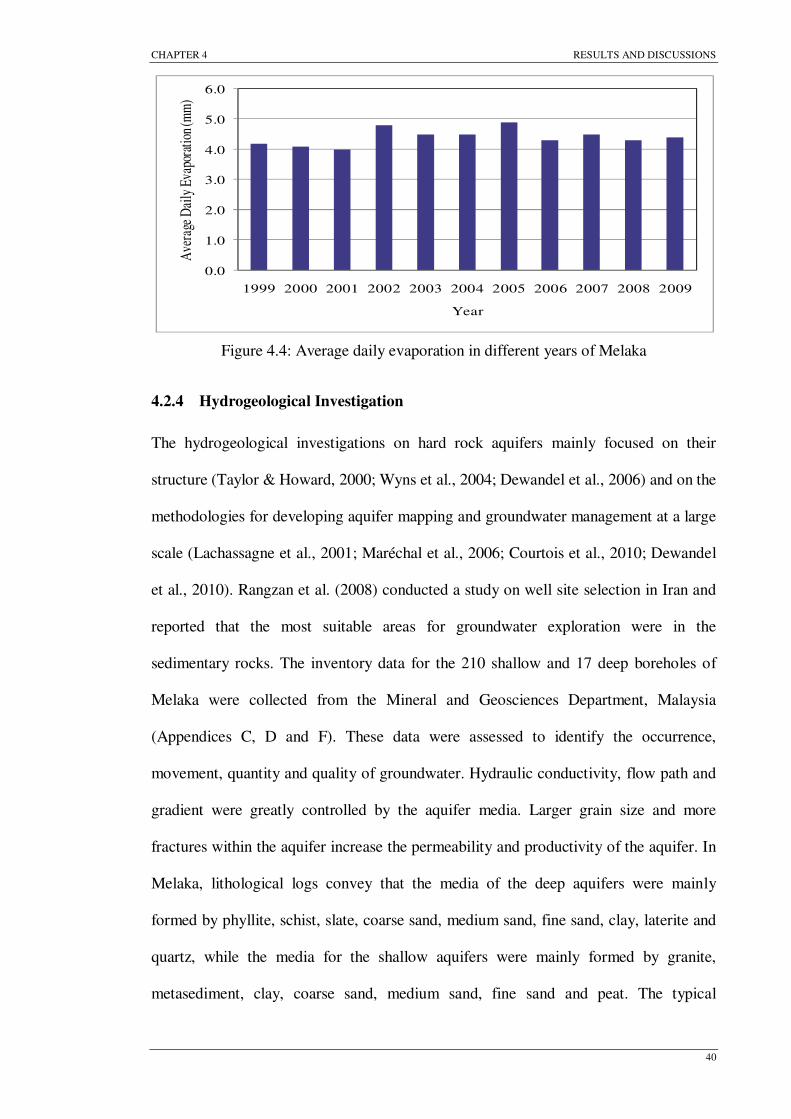
CHAPTER 4 RESULTS AND DISCUSSIONS
40
Figure 4.4: Average daily evaporation in different years of Melaka
4.2.4 Hydrogeological Investigation
The hydrogeological investigations on hard rock aquifers mainly focused on their
structure (Taylor & Howard, 2000; Wyns et al., 2004; Dewandel et al., 2006) and on the
methodologies for developing aquifer mapping and groundwater management at a large
scale (Lachassagne et al., 2001; Maréchal et al., 2006; Courtois et al., 2010; Dewandel
et al., 2010). Rangzan et al. (2008) conducted a study on well site selection in Iran and
reported that the most suitable areas for groundwater exploration were in the
sedimentary rocks. The inventory data for the 210 shallow and 17 deep boreholes of
Melaka were collected from the Mineral and Geosciences Department, Malaysia
(Appendices C, D and F). These data were assessed to identify the occurrence,
movement, quantity and quality of groundwater. Hydraulic conductivity, flow path and
gradient were greatly controlled by the aquifer media. Larger grain size and more
fractures within the aquifer increase the permeability and productivity of the aquifer. In
Melaka, lithological logs convey that the media of the deep aquifers were mainly
formed by phyllite, schist, slate, coarse sand, medium sand, fine sand, clay, laterite and
quartz, while the media for the shallow aquifers were mainly formed by granite,
metasediment, clay, coarse sand, medium sand, fine sand and peat. The typical
0.0
1.0
2.0
3.0
4.0
5.0
6.0
1999 2000 2001 2002 2003 2004 2005 2006 2007 2008 2009
Ave
rage
Dai
ly E
vapo
ratio
n (m
m)
Year

CHAPTER 4 RESULTS AND DISCUSSIONS
41
lithological formations of the study area are presented in Figures 4.5 and 4.6 for deep
and shallow aquifers, respectively.
Figure 4.5: Typical lithology of deep aquifers in Melaka
Figure 4.6: Typical lithology of shallow aquifers in Melaka

CHAPTER 4 RESULTS AND DISCUSSIONS
42
4.2.5 Pump Test and Aquifer Productivity
Based on the preliminary field survey and collected pump test data of Melaka, it is
possible to provide an overview of the groundwater condition of the study area
(Appendices C, D and F). The Productivity of the aquifer in the study area was tested by
pumping tests and deep drilling. The term ‘aquifer productivity’ represents the potential
of an aquifer to sustain various levels of borehole supply. Pumping test data were used
to determine the aquifer parameters in order to ensure the aquifer potentiality (Patra et
al., 1993; Singhal et al., 1998). The pump tests results of Melaka showed that the study
area was largely dominated by phyllite, slate, schist and granite. The rock type in each
borehole was categorized from the pump test data and hydrogeological map.
The aquifer productivity classifications are presented in Table 4.1 based on the
judgments of the typical long-term discharge rate in cubic meter per hour from the
reliable site and constructed boreholes. It is a comparative classification of productivity
among the boreholes of the study area. The aquifer productivity is classified by having a
typical yield ranges of <3.6 m3/h (low), 3.6-12 m3/h (moderate) and >12 m3/h (high).
Table 4.1: Aquifer productivity classification of the State of Melaka
District Total No.
of Boreholes
No. of Active
Boreholes
Productivity Classes Area (%)
Total Dischar
ge (m3/h)
High (>12 m3/h)
Moderate (3.6-12 m3/h)
Low (<3.6 m3/h)
Alor Gajah
80 5 12.3-18 8
274 31 3.6-12 54 22 0.2-3.5 38
Melaka Tengah
107
2 13.5-18 4
138 36 4-8.2 68 15 0.5-3.5 28
Jasin 71 5 13.6-18 10
211 24 4-12 50
19 0.5-3.5 40 * The productivity rating refers to the estimated typical long-term yield from properly sited and
constructed boreholes of the study area.

CHAPTER 4 RESULTS AND DISCUSSIONS
43
Investigation in the area of Alor Gajah indicated that the bedrock of shallow aquifers
was governed by phyllite, schist and granite. About 73 shallow boreholes gave different
discharge results. Most of the boreholes discharge was 3.6-12 m3/h and the discharge of
only a few shallow and deep aquifers gave a satisfactory result (>12 m3/h).
Groundwater potentiality was limited in the region of Central Melaka based on
lithology data and pump test. Among the 107 units, only 53 drill holes discharged at
138 m3/h. Moderate productivity aquifers were composed of phyllite, schist, and slate
which is a thin layer of metamorphic rock that is easily split. This layer has lower
permeability than the well-sorted, coarser and high productivity deposits that reduces
their potential for yielding large volumes of groundwater. Granite and acid intrusive
rocks were dominant in the low productivity aquifer bedrock which was not suitable for
the storage of groundwater.
The high potentiality of groundwater in the Jasin area had found in the schist, sand,
limestone and volcanic rocks region. Among the 63 shallow boreholes, it was possible
to extract groundwater from 50. The ranges of discharge of the most aquifers were 0.5-
12 m3/h. The discharge capacity of the aquifers was tested by drilling deep to find out
the value of the transmissivity coefficient (T) and hydraulic conductivity (K). A
pumping test was continuously carried out for 6 hours, before waiting for the
groundwater elevation to rise. The results were found to be 10m2/day for the
transmissivity coefficient (T) and 0.63 m/day for the hydraulic conductivity (K). The
aquifer productivity results for groundwater potential at Melaka indicated that 35% area
is low, 57% is moderate and 8% is high. The potential zones and existing well locations
in the study area are presented in Figure 4.7.

CHAPTER 4 RESULTS AND DISCUSSIONS
44
Figure 4.7: Well locations and aquifer potential map of Melaka
4.3 Preparation of DRASTIC Parameter Maps
Seven thematic maps are generated based on hydrogelogical settings (Appendices B-D
and F) to carry out the aquifer vulnerability assessment using the DRASTIC method
and GIS. DRASTIC method mainly comprises two factors; hydrogeological settings
and relative ranking of the parameters. The method is considered the generic pollutant
rather than specifics of the particular pollutant. The successive steps for preparing the
thematic maps for the DRASTIC parameters have been described in following order to
generate the final vulnerability map of groundwater.
4.3.1 Groundwater Depth
The depth of water table is defined as the distance in which the pollutants move through
the soil media before reaching the groundwater table. If depth to water table increases, it
facilitates the significant contaminant attenuation as the contaminant needs to travel
long distance and get enough time to contact with flow media. Depth of groundwater is

CHAPTER 4 RESULTS AND DISCUSSIONS
45
also important for oxidation process by atmospheric oxygen. Hence, the pollutant
elapsed time and attenuation depends on the soil media and the depth to the water table,
which has a significant effect on assigning the rating value of the parameter. Depth to
water table was calculated from the each groundwater level data and the well location.
The respective information was collected from boreholes log information, existing
groundwater level from shallow aquifers and drilling wells. The values of groundwater
depth are used to compute the rates according to the categories, which are summarized
in Table 4.2 and relevant information in Figure 4.8. The figure showed that the depth to
groundwater table distance was very low (1.0 m) along the bank of the Melaka Straight
and the depth increases from bank to the inland, where maximum water depth was 5
meters. The high rating value was assigned for shallow aquifer around the bank of
Melaka straight, while comparatively less rating value was assigned for the remaining
area due to increase distance of groundwater table.
Figure 4.8: Depth to groundwater map of Melaka

CHAPTER 4 RESULTS AND DISCUSSIONS
46
Table 4.2: DRASTIC parameter rating and weighting values
Rating D x (5) Depth of Water (m)
R x (4) Net Recharge (mm/year)
A x (3) Aquifer Media
10 0-1.5 Krast limestone 9 1.5-4.5 >250 Basalt 8 180-250 Sand and gravel 7 4.5-9.0 Massive sandstone, massive
limestone 6 100-180 Bedded sandstone, limestone, shale 5 9-15 Glacial 4 Weathered metamorphic / igneous 3 15-23 50-100 Metamorphic / igneous 2 23-31 Massive shale 1 >31 0-50 -
4.3.2 The Recharge
The net recharge is defined as the amount of water that reached into the groundwater
system resulting from the precipitation and artificial sources available. The recharge is
controlled by land cover, slope, rainfall, permeability of soil, drainage system and
lithological conditions. Recharge water a significant vehicle to percolating and
transferring of contaminants into the groundwater system. The dispersion and dilution
of pollutants in the vadose zone and saturated are controlled by net recharge. High
recharge indicates the high pollution potential to contamination. The groundwater
pollution and potentiality depend on the rate of net recharge through the faults and
fractures (Travaglia & Dainelli, 2003). In the study area, the shallow aquifers were
subjected to high recharge, which was mainly governed by precipitation. Most of the
cases, shallow aquifers recharged by direct rainfall, and recharge rate were greater than
the deep aquifers. The recharge map is generated from the rainfall data and using the
following Equation (4.1):
Net Recharge = (Rainfall - Evaporation) × Coefficient of Thiessen......................... (4.1)

CHAPTER 4 RESULTS AND DISCUSSIONS
47
In the Thiessen method (Thiessen and Alter, 1911), all the gauge locations are plotted
on the map at an appropriate scale. Next, the straight lines are drawn to connect the
gauges without crossing any other lines. Each connecting line is then bisected and a
perpendicular line is drawn through the connecting line. Each gauge is near the center
of a polygon whose size varies according to the spacing of the gauges. The area of each
polygon is then measured. The Coefficient of Thiessen is defined as the ratio between
the individual polygon area and the summation of all the polygon area. The 22 years
mean of annual rainfall (mm/year) and evaporation (mm/year) data were used to prepare
the recharge map based on Thiessen method. The net recharge distribution map is
presented in Figure 4.9 and respective information in Table 4.2. The map illustrated that
most parts of Melaka and East parts of the Alor Gajah district were subjected to high
recharge ranges from 475-714 mm/yr, mainly formed by Phyllite, Schist, Slate and
granite, while major part of Jasin district showed the recharge range from 382-474
mm/yr, formed by Schist, Sand, Limestone, Igneous rock and Granite. The remaining
area was under comparatively less recharge and mostly affected by high land.
Figure 4.9: Net recharge map of the study area

CHAPTER 4 RESULTS AND DISCUSSIONS
48
4.3.3 Aquifer Media
An aquifer is defined as a subsurface rock unit which will yield sufficient quantities of
water for use. It also defines the consolidated and unconsolidated rock, in which water
contained by fractures and pore spaces. Aquifer media controls the water flow through
the aquifers. The rate of contaminant transformation is controlled by flow path (Aller, et
al., 1987). Aquifer media has significant effect to control hydraulic conductivity as well
as contaminant attenuation process such as sorption and dispersion to occur while
contaminants pass through it. In order to assess the impact of the aquifer media on the
vulnerability of groundwater resources, GIS database are prepared from the data of
subsurface lithology. Each media is rated and weighted according to their relative
importance to contamination. Based on the number of 238 shallow and 20 deep
boreholes available data, the aquifer media map is generated which is shown in Figure
4.10 with relevant rating information in Table 4.2. The figure showed that the aquifer
media of the study area was mostly formed by Phyllite and its rating value assigned as
2. Second major formation was Acid Intrusive rock and third was Shale, Mudstone and
Siltstone, which rating values assigned 5 and 7, respectively due to their high porosity
and fracture characteristics for water storage.
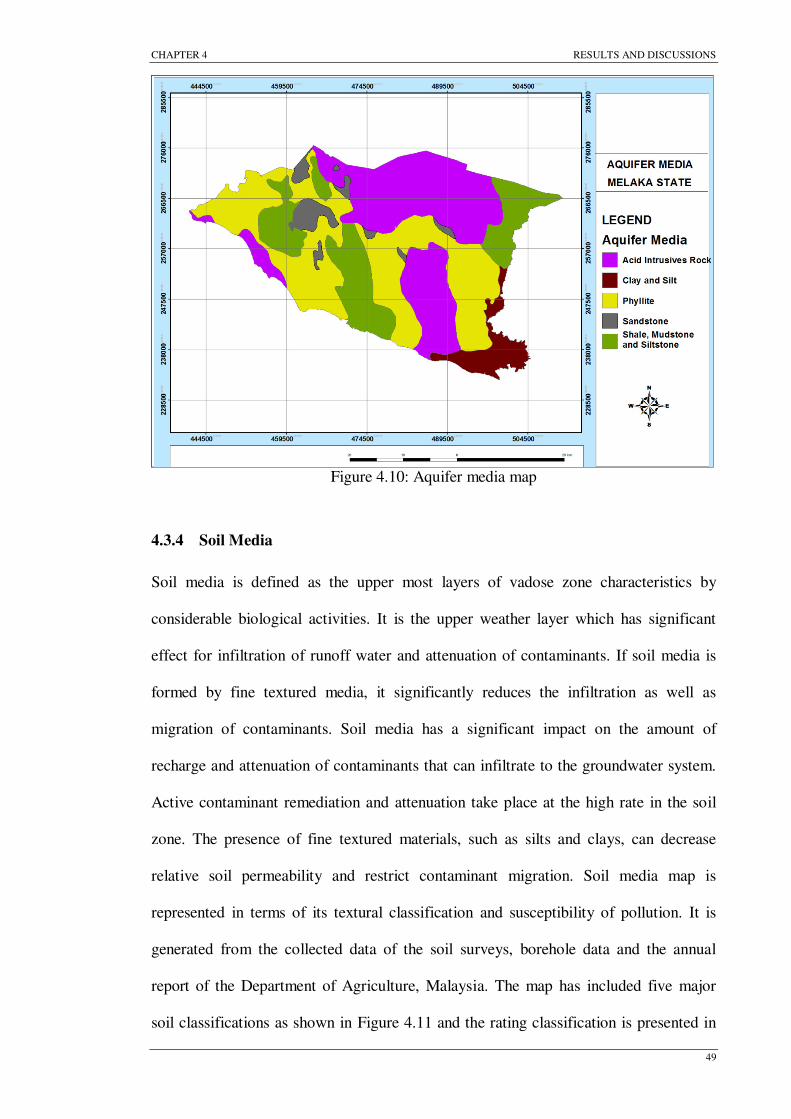
CHAPTER 4 RESULTS AND DISCUSSIONS
49
Figure 4.10: Aquifer media map
4.3.4 Soil Media
Soil media is defined as the upper most layers of vadose zone characteristics by
considerable biological activities. It is the upper weather layer which has significant
effect for infiltration of runoff water and attenuation of contaminants. If soil media is
formed by fine textured media, it significantly reduces the infiltration as well as
migration of contaminants. Soil media has a significant impact on the amount of
recharge and attenuation of contaminants that can infiltrate to the groundwater system.
Active contaminant remediation and attenuation take place at the high rate in the soil
zone. The presence of fine textured materials, such as silts and clays, can decrease
relative soil permeability and restrict contaminant migration. Soil media map is
represented in terms of its textural classification and susceptibility of pollution. It is
generated from the collected data of the soil surveys, borehole data and the annual
report of the Department of Agriculture, Malaysia. The map has included five major
soil classifications as shown in Figure 4.11 and the rating classification is presented in

CHAPTER 4 RESULTS AND DISCUSSIONS
50
Table 4.3. The map clearly indicates that the soil media mainly formed by Phyllite,
Schist and Slate in the major parts of the study area and its rating value was assigned 5,
while the maximum rating values were assigned as 7 and 9 for Alluvium and Volcanic
rocks, respectively.
Table 4.3: Rating values of soil media in the study area
Rating
S x (2)
Soil media
10 Thin or absent, gravel 9 Sand stone and volcanic 8 Peat 7 Shrinking and/or aggregate clay/Alluvium 6 Sandy loam, sys, sand, karts, volcanic 5 Loam 4 Silty loam 3 Clay loam 2 Muck, acid , granitoid 1 Non shrink and non-aggregated clay
Figure 4.11: Soil media map
CHAPTER 4 RESULTS AND DISCUSSIONS
51
4.3.5 Topography
Topography is defined as the slope discrepancy of land surface. Precipitation and
pollutant infiltration rate into groundwater are greatly controlled by the degree of the
slope. The degree of slope dictates where the precipitation will retain or run off on the
surface. On the similar manner, the contaminants will also leave its position as run off
or percolate into ground or eventually reach into the groundwater table (Brady & Weil,
2004). Generally, runoff is channeled out from higher to lower elevation and make the
lower area is more vulnerable. The topography in the DRASTIC method implies the
slope of the ground surface in percentage and is shown in Figure 4.12. In order to
compute the slope, the digital elevation model (DEM) of the Melaka catchment was
used through the GIS environment. There is a readily available option in the Spatial
Analyst of GIS, where it is straightforward to compute the slope of the ground surface
from the grid of the DEM. The relevant slope classification is presented in Table 4.4.
Topography map demonstrated that the slope range of the study area was very low
mostly laid from 0-5 percent. So, it had significant threat for groundwater
contamination, in which its rating values were assigned as high range between 7 and10.
Figure 4.12: Topography map

CHAPTER 4 RESULTS AND DISCUSSIONS
52
4.3.6 Impact of Vadose Zone
Vadose zone is defined as the unsaturated layer above the groundwater table which is
discontinuously saturated. The impact of vadose zone provides the first line natural
defense against the contaminants to pass into the groundwater system. It controls the
passage and attenuation of the contaminant into the aquifer. This zone is increased the
significant travel time of the contaminants before reaching the groundwater system. The
vadose zone has a significant effect to diminution groundwater pollution, because some
pollutant attenuation processes occur in this layer such as biodegradation, filtration,
mechanical straining, chemical reaction and dispersion (Piscopo, 2001). The impact of
vadose zone map is presented in Figure 4.13 and the relevant rating ranges are shown in
Table 4.4. The vadose zone formed by fine granite and gravel sand-clay mostly covered
the study area and the rating values were assigned as 8 and 6, respectively because of
their coarse texture formation, while another major formation of vadose governed by
Granite and its assigned rating was 1 due to the insufficient opportunities for occurring
some attenuation process through the media.
Figure 4.13: Vadose zone map

CHAPTER 4 RESULTS AND DISCUSSIONS
53
4.3.7 Hydraulic Conductivity
Hydraulic conductivity indicates the movement rate of groundwater through the
saturated zone and transport contaminants into groundwater system. It represents the
transfer speed of water through the aquifer of groundwater system. Contaminant
percolation tendency is controlled within this zone. Only vertical conductivity was
considered to assess the vulnerability, where higher rate conductivity indicates higher
pollution potential. The hydraulic conductivity map (Figure 4.14) was generated from
the pumping test data of 20 deep wells and improved after calibration of the
mathematical model in steady state. The vertical hydraulic conductivities of the aquifer
materials in the study area are commonly less than 1m/day and considered the constant
rating value one (1) through the whole study area which is shown in Figure 4.14 and
relevant classifications are shown in Table 4.4.
Table 4.4: DRASTIC quantitative parameters
T x ( 1 ) I x ( 5 ) C x ( 3 )
Rating Topography
(%) Vadose zone media
Hydraulic conductivity (m/s)
10 0 - 2 Karst limestone > 9.5×10⁻⁴ 9 2 - 3 Basalt 7 ×10⁻⁴ – 9.5×10⁻⁴ 8 3 – 4 Sand and gravel 5×10⁻⁴ – 7 ×10⁻⁴
7 4 – 5 Gravel and sand with silt and clay 20 ×10-4 – 5×10⁻⁴
6 5 – 6 Limestone, sandstone, slate 30×10-5 – 20×10-4 5 6 – 10 Sandy silt 20 ×10-5 – 30×10-5 4 10 -12 Metamorphic/ Igneous 15×1-5 – 20×10-5 3 12 – 16 Shale, silt, and clay 10 ×1-5– 15×10-5 2 16 - 18 Silt/clay 5×10⁻⁵ – 10×10-5
1 > 18 Confining layer, biotic- granite 1.5×10⁻⁷ – 5×10⁻⁵

CHAPTER 4 RESULTS AND DISCUSSIONS
54
Figure 4.14: Hydraulic conductivity map
4.3.8 Final Vulnerability Map
The seven hydro-geological parameters were deemed important to generate final
DRASTIC vulnerability map. The GIS coverage was all in raster format and the values
for each overlay are assigned according to the pixel value of each area that resulted
from multiplying the ratings with its appropriate DRASTIC weight. Combining the
hydrogeological setting results in a range of numerical values termed the DRASTIC
Index. Derived by combining the seven DRASTIC element index values, a range of
values are developed that have been classified to represent groundwater vulnerability.
These numbers are relative and have no intrinsic meaning other than in comparison with
other like DRASTIC indices. The classification scheme is implemented based on the
statistical grouping of DRASTIC index values. In order to maximize the difference
between classes, a Natural Breaks method is chosen for identifying areas that fall within
a low, medium, or high vulnerability region. The minimum and maximum range of

CHAPTER 4 RESULTS AND DISCUSSIONS
55
DRASTIC index was found as 23 and 230, respectively and classified into four classes
such as very low, low, moderate and high (Aller, et al., 1987). In this study, the resulted
DRASTIC index values laid between 80 and 185. Therefore, the DRASTIC index
values are classified into three categories namely;- high vulnerability (>159), moderate
vulnerability (120-159) and low vulnerability (80-119). The range of classifications and
the affected area categorization are presented in Table 4.5. The classifications ranges
are arbitrary and the corresponding categories can be varied which depend on the
personal judgment of the researcher.
Table 4.5: Conventional DRASTIC index classification of the study area
DRASTIC index DRASTIC range % of the area High vulnerability > 159 27.45 Moderate vulnerability 120–159 61.53 Low vulnerability 80–119 11.02
The final DRASTIC groundwater vulnerability map (Figure 4.15) is clearly indicated
that only a very small portion of the study area (North) is subjected to low vulnerability
(11.02%) which is high land, and major parts of the study area shows moderate
vulnerability to contamination (61.53%) is affected by agricultural and urban activities
as well as found high groundwater level along the bank of Melaka Straight and its
surrounding area. The area which is marked as high vulnerability (27.45%) to
contamination falls in and around Melaka, Jasin and Alor Gajah Cities. These areas are
threatened by high permeable and locally high recharge unconfined shallow aquifers.
Wastewater is resulted from the urban and industrial activities of the Melaka, Jasin and
Alor Gajah cities have significant effect to increase the high vulnerability of
groundwater surrounding the city areas.

CHAPTER 4 RESULTS AND DISCUSSIONS
56
Figure 4.15: The DRASTIC aquifer vulnerability map
4.4 Final Risk Map
The risk map is generated using the modified DRASTIC method based on land use
category, which indicates the area where anthropogenic activities is more liable for the
groundwater vulnerability in the study area. The risk map is classified into three
categories; low (100-139), moderate (140-175) and high (>175) vulnerability that is
presented in Table 4.6, whereas the classification concepts are same as final
vulnerability classification system.
Table 4.6: Modified DRASTIC index classification of the study area
MDI MDI range % of the area
High vulnerability > 175 38.26 Moderate vulnerability 140–175 47.34 Low vulnerability 100–139 14.40
The results of the analysis show that 38.26% of the area is high vulnerability, 47.34%
moderate vulnerability and 14.40% low vulnerability as presented in Figure 4.16. The
risk map indicates that high vulnerability area is increased more than 11% while

CHAPTER 4 RESULTS AND DISCUSSIONS
57
moderate vulnerability decreases around 14% compare to conventional DRASTIC
vulnerability map. The comparison of risk map and land use map clearly indicates that
the areas which are greatly affected by urban, industrial, agricultural, short term crop
land, animal husbandry and horticultural activities are showed the high vulnerability of
groundwater. Palm oil tree and other permanent crops are available in the moderate
vulnerability zone. Therefore, it indicates the main adverse effects on the groundwater
system are resulted from the agricultural, industrial and urban activities. The most
hazards exist around the Melaka, Jasin and Alor Gajah cities due to the infiltration of
urban and industrial waste water. Sea water intrusions also have significant effect to
increase the groundwater vulnerability of coastal and its surrounding region.
Figure 4.16: Modified DRASTIC aquifer vulnerability map

CHAPTER 4 RESULTS AND DISCUSSIONS
58
4.5 Validation of the DRASTIC Method
For the purpose of DRASTIC model validation, two groundwater quality parameters
such as nitrate and chloride are used as a controlling parameter. In natural condition,
nitrate is not generally present in groundwater. Usually it infiltrates from ground
surface. Therefore, it is more effective indicating parameter to represent the
groundwater contamination, where contaminants transport by infiltrate water from the
ground surface into groundwater system. Nitrate and chloride parameter are used to
develop the correlations with the values of conventional and modified DRASTIC index,
respectively. Correlation is a technique for investigating the relationship between two
quantitative, continuous variables. The linear correlation coefficient measures the
strength and the direction of a linear relationship between two variables. The linear
correlation coefficient is sometimes referred to as the Pearson product moment
correlation coefficient in honor of its developer Karl Pearson (Pearson, 1900).
In this study, the correlations are established based on Pearson's correlation method and
the SPSS software was used to develop the correlations. The required data such as
Nitrate and Chloride concentration values as well as conventional DRASTIC index (DI)
and modified DRASTIC index (MDI) values which are used to establish the
correlations as shown in Table 4.7. Firstly, DI and MDI values are used to establish the
correlation with Nitrate concentration values. The correlation coefficient values are
found 0.772 and 0.82 for the DI and MDI which represent the strong correlations with
them as shown in Tables 4.8 and 4.9. Secondly, Chloride concentration values are used
to make the correlation with DI and MDI values and found the coefficient values 0.617
and 0.695, respectively which also show the good correlations between the parameters
as shown in Tables 4.10 and 4.11.

CHAPTER 4 RESULTS AND DISCUSSIONS
59
Table 4.7: Correlation data for the DRASTIC method validation
Observation No.
NO3 Concentration (mg/l)
Cl Concentration (mg/l)
DI MDI
1 1 1 90 100 2 1 1 94 102 3 1 1 99 103 4 1 1 103 104 5 1 2 105 106 6 1 2 107 107 7 1 2 109 110 8 3 2 110 111 9 3 2 112 114
10 3 3 113 116 11 3 3 115 120 12 3 4 118 125 13 3 4 119 126 14 3 5 120 130 15 3 5 122 132 16 3 6 125 136 17 3 6 126 137 18 3 6 127 138 19 3 6 129 140 20 3 7 130 141 21 3 7 132 143 22 3 8 133 144 23 3 10 135 146 24 4 12 137 148 25 4 13 138 149 26 4 13 139 150 27 4 14 140 151 28 4 14 142 155 29 4 16 144 157 30 4 16 146 160 31 7 17 148 163 32 7 17 149 164 33 7 27 150 165 34 8 30 151 166 35 8 120 153 170 36 9 175 154 171 37 9 225 157 175 38 9 445 158 177 39 12 445 159 180 40 12 1025 161 185 41 13 1025 162 185 42 13 1750 165 190 43 13 1750 167 205 44 32 2200 173 210

CHAPTER 4 RESULTS AND DISCUSSIONS
60
Table 4.8: Correlation between Nitrate concentration and DRASTIC Index
Nitrate DI
Nitrate
Pearson Correlation 1 0.772**
Sig. (2-tailed) 0.000
N 44 44
DI
Pearson Correlation 0.772** 1
Sig. (2-tailed) 0.000
N 44 44
**. Correlation is significant at the 0.01 level (2-tailed).
Table 4.9: Correlation between Nitrate concentration and Modified DRASTIC Index
Nitrate MDI
Nitrate
Pearson Correlation 1 0.820**
Sig. (2-tailed) 0.000
N 44 44
MDI
Pearson Correlation 0.820** 1
Sig. (2-tailed) 0.000
N 44 44
**. Correlation is significant at the 0.01 level (2-tailed).
Table 4.10: Correlation between Chloride concentration and DRASTIC Index
Chloride DI
Chloride
Pearson Correlation 1 0.617**
Sig. (2-tailed) 0.000
N 44 44
DI
Pearson Correlation 0.617** 1
Sig. (2-tailed) 0.000
N 44 44
**. Correlation is significant at the 0.01 level (2-tailed).
Table 4.11: Correlation between Chloride concentration and Modified DRASTIC Index
Chloride MDI
Chloride
Pearson Correlation 1 0.695**
Sig. (2-tailed) 0.000
N 44 44
MDI
Pearson Correlation 0.695** 1
Sig. (2-tailed) 0.000
N 44 44
**. Correlation is significant at the 0.01 level (2-tailed).

CHAPTER 4 RESULTS AND DISCUSSIONS
61
The correlation coefficients are found 77% between nitrate concentrations and
conventional DRASTIC index values, and 82% between nitrate concentrations and
modified DRASTIC index values. Again, correlation coefficient is found 62% between
chloride concentrations and conventional DRASTIC index values as well as 70 %
between chloride concentrations and modified DRASTIC index values. In conclusion,
Minitab’s (Tables 4.9-4.12) from SPSS analysis output indicates that the strength of
association between the variables is moderate to high (r = 0.62-0.82), and the
correlation coefficient is high significantly different from zero (P < 0.001). All
correlation coefficients are statistically significant at 99% confidence level according to
Pearson's correlation method.
4.6 Groundwater Quality
Water quality is the most important issue for all living beings and different sectors of
use. The chemical composition of groundwater in bedrock often varies greatly from the
superficial drift deposit. The groundwater from bedrock is often more natural, more
basic, more reducing, more sodium-rich and contains more of most of the minor/trace
elements than drift groundwater. The 52 shallow and 14 deep boreholes groundwater
quality data were collected from Mineral and Geo-science Department (Appendix G)
and analyzed for major cations (Ca2+, Mg2+, Na+, Fe 2+, Mn+2 and K+) and anions
(HCO3-, SO2-
4 and Cl-). Other physico-chemical parameters like conductivity, pH, total
dissolved solids and turbidity were also measured. The different groundwater quality
parameter values are presented in the form of histograms from Figures 4.17 to 4.26 for
shallow and deep boreholes. The histograms represent the concentration values and its
frequency of individual groundwater quality parameter. The various groundwater
quality parameters of the study area are analyzed and mentioned its present state. The
groundwater quality of Central Melaka is in good condition and can be used as raw

CHAPTER 4 RESULTS AND DISCUSSIONS
62
water in accordance with the requirements based on the raw water quality standards by
the Ministry of Health Malaysia (Appendix E). However, some places, such as Mukim
Keeling, Cheng, Ayer Molek and Cage experience salty and brackish conditions as a
result of seawater intrusion. The groundwater is affected by the brackish nature in the
coastal region due to the seawater influence and hydrogeochemical process (Bahar &
Reza, 2010). The quality of ground water in Alor Gajah district is still eligible as a
source of water for residents. The quality of groundwater, particularly in the coastal
areas of Kuala Linggi is still contaminated by salt water due to the intrusion of
seawater. Over pumping and decreasing recharge rate causes aquifer depletion and leads
to the intrusion of seawater (Moustadraf et al., 2008; Pujari & Soni, 2008; Zhou, 2009).
Commonly, the coastal areas of this region are subjected to the brackish and salty
conditions located both on the alluvium stone and hard rock stone.
The groundwater quality analysis indicated that turbidity, total dissolved solids, iron,
chloride and cadmium values were high for both shallow and deep boreholes in few
parts of the study area. The pH values of shallow boreholes indicated that around 50%
of water samples were between 4-6.5 and the remaining 50% of water samples were
between 6.5 and 8.2. Again, the pH values of the deep boreholes indicated that about
50% of the samples were around 5.2 and the remaining 50% were between 6.7 and 8.5.
The high TDS values indicated that the groundwater was affected by the percolation of
agricultural, industrial and residential runoff water. The statistical analysis of different
water quality parameter values are presented in Tables 4.12 and 4.13 for shallow and
deep boreholes, respectively. The statistical results indicated that Conductivity, TDS,
Na, Cl and SO4 concentration values abruptly varies for shallow aquifer as well as for
deep aquifer except SO4. On the otherhand, pH, CO3, Cd and P values for shallow
aquifer and pH, NO3-N, Fe, K, Cd values for deep aquifer showed very close
differences, in which water samples collected from different boreholes of the study area.

CHAPTER 4 RESULTS AND DISCUSSIONS
63
Figure 4.17: Turbidity values in shallow and deep boreholes
Figure 4.18: Total dissolved solids values in shallow and deep boreholes
Figure 4.19: pH values in shallow and deep boreholes
S= Shallow borehole, D= Deep borehole,
0
2
4
6
8
10
12
14
16
5 15 25 35 45 60 80 100 120 140 160 180 200
Fre
quen
cy
Turbidity (NTU)
S D
0
1
2
3
4
5
6
7
20
60
100
140
180
220
260
300
340
380
420
760
800
840
880
920
960
1000
2000
3000
4000
Fre
quen
cy
Total dissolved solids (mg/l)
S D
0
5
10
15
20
25
4 5.5 6 7 8 8.5 10
Fre
quen
cy
pH
S D
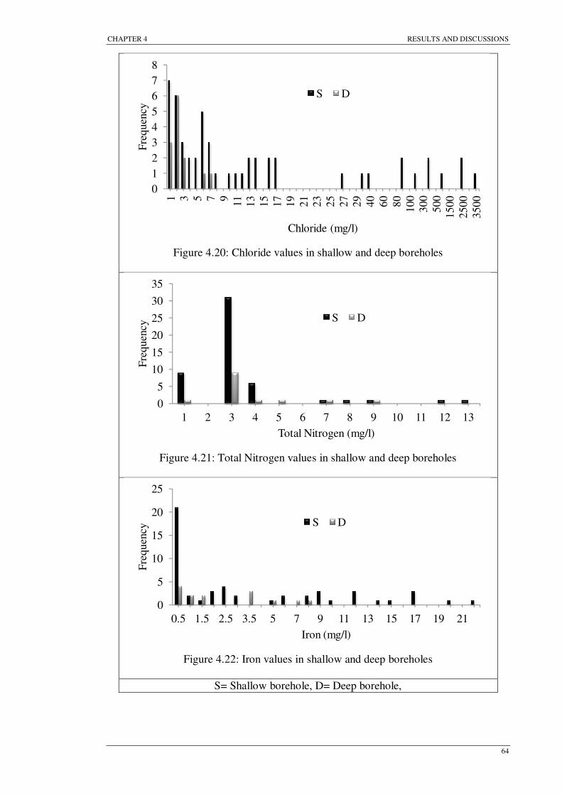
CHAPTER 4 RESULTS AND DISCUSSIONS
64
Figure 4.20: Chloride values in shallow and deep boreholes
Figure 4.21: Total Nitrogen values in shallow and deep boreholes
Figure 4.22: Iron values in shallow and deep boreholes
S= Shallow borehole, D= Deep borehole,
0
1
2
3
4
5
6
7
8
1 3 5 7 9
11 13
15
17
19
21
23
25
27
29
40
60
80
100
300
500
1500
2500
3500
Fre
quen
cy
Chloride (mg/l)
S D
0
5
10
15
20
25
30
35
1 2 3 4 5 6 7 8 9 10 11 12 13
Fre
quen
cy
Total Nitrogen (mg/l)
S D
0
5
10
15
20
25
0.5 1.5 2.5 3.5 5 7 9 11 13 15 17 19 21
Fre
quen
cy
Iron (mg/l)
S D

CHAPTER 4 RESULTS AND DISCUSSIONS
65
Figure 4.23: Sodium values in shallow and deep boreholes
Figure 4.24: Sulphate values in shallow and deep boreholes
Figure 4.25: Cadmium values in shallow and deep boreholes
S= Shallow borehole, D= Deep borehole,
0
1
2
3
4
5
6
7
1 3 5 7 9 11 13
15
17
19
30
50
70
90
150
250
350
450
1000
Fre
quen
cy
Sodium (mg/l)
S D
0
2
4
6
8
10
12
14
16
1 3 5 7 9 11 13 15 25 35 45 100 200 300
Fre
quen
cy
Sulphate (mg/l)
S D
0
5
10
15
20
25
30
35
0.01 0.02 0.03 0.04 0.05 0.1
Fre
quen
cy
Cadmium (mg/l)
S D
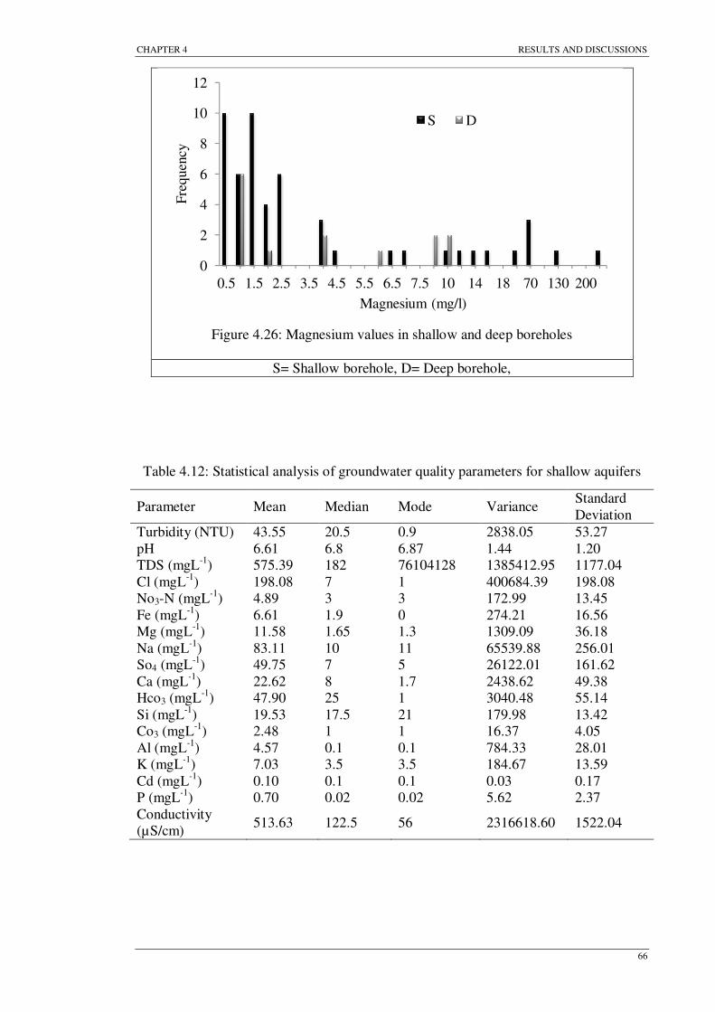
CHAPTER 4 RESULTS AND DISCUSSIONS
66
Figure 4.26: Magnesium values in shallow and deep boreholes
S= Shallow borehole, D= Deep borehole,
Table 4.12: Statistical analysis of groundwater quality parameters for shallow aquifers
Parameter Mean Median Mode Variance Standard Deviation
Turbidity (NTU) 43.55 20.5 0.9 2838.05 53.27 pH 6.61 6.8 6.87 1.44 1.20 TDS (mgL-1) 575.39 182 76104128 1385412.95 1177.04 Cl (mgL-1) 198.08 7 1 400684.39 198.08 No3-N (mgL-1) 4.89 3 3 172.99 13.45 Fe (mgL-1) 6.61 1.9 0 274.21 16.56 Mg (mgL-1) 11.58 1.65 1.3 1309.09 36.18 Na (mgL-1) 83.11 10 11 65539.88 256.01 So4 (mgL-1) 49.75 7 5 26122.01 161.62 Ca (mgL-1) 22.62 8 1.7 2438.62 49.38 Hco3 (mgL-1) 47.90 25 1 3040.48 55.14 Si (mgL-1) 19.53 17.5 21 179.98 13.42 Co3 (mgL-1) 2.48 1 1 16.37 4.05 Al (mgL-1) 4.57 0.1 0.1 784.33 28.01 K (mgL-1) 7.03 3.5 3.5 184.67 13.59 Cd (mgL-1) 0.10 0.1 0.1 0.03 0.17 P (mgL-1) 0.70 0.02 0.02 5.62 2.37 Conductivity (µS/cm)
513.63 122.5 56 2316618.60 1522.04
0
2
4
6
8
10
12
0.5 1.5 2.5 3.5 4.5 5.5 6.5 7.5 10 14 18 70 130 200
Fre
quen
cy
Magnesium (mg/l)
S D

CHAPTER 4 RESULTS AND DISCUSSIONS
67
Table 4.13: Statistical analysis of groundwater quality parameters for deep aquifers
Parameter Mean Median Mode Variance Standard Deviation
Turbidity (NTU) 14.06 9.2 1 242.30 15.57 pH 6.66 6.7 5.2 1.86 1.36 TDS (mgL-1) 1210.73 196 36285480 11539996 8897.05 Cl (mgL-1) 74.60 2 2 79687.31 282.29 No3-N (mgL-1) 3.92 3 3 9.72 3.12 Fe (mgL-1) 1.83 0.5 0.1,0.5 6.07 2.46 Mg (mgL-1) 8.74 2.4 0.1 443.69 21.06 Na (mgL-1) 148.6 7.4 12 194558.53 441.08 So4 (mgL-1) 40.29 4 1 8788.06 40.29 Ca (mgL-1) 44.21 14 11 3822.74 44.21 Hco3 (mgL-1) 76.72 18 5 8180.66 90.44 Si (mgL-1) 18 10 1 626.88 25.03 Co3 (mgL-1) 6.89 1 1 395.53 19.89 Al (mgL-1) 20.42 0.1 0.1 3698.43 60.81 K (mgL-1) 3.05 1 0.01 13.88 3.73 Cd (mgL-1) 1.17 0.02 0.01 8.40 2.90 P (mgL-1) 25.49 0.025 0.02 5479.25 74.02 Conductivity (µS/cm)
355.80 55 5 870428.30 932.96

CHAPTER 5 CONCLUSIONS AND RECOMMENDATIONS
68
Chapter 5
CONCLUSIONS AND RECOMMENDATIONS
5.1 General
The research findings, various issues and discussions have been placed in the previous
chapters. The methodologies, assessment and necessary discussion are placed there.
This chapter summarizes the research findings and recommends for further research
directions.
5.2 Summary and Conclusions
[a] The analysis of the hydraulic conductivity, transmissivity and aquifers yield
results indicates that the aquifers formed by schist, sand, limestone as well as
volcanic rocks are the most productive for groundwater.
[b] Groundwater potentiality is satisfactory in most places underlaid by phyllite,
schist and slate. This reason may first, be because the bedrock is fractured, and
second, because of the high recharge rate due to available rainfall.
[c] The productivity of the aquifer is classified by having a typical yield ranges of
<3.6 m3/h (low), 3.6-12 m3/h (moderate) and >12 m3/h (high). From the view of
aquifer productivity, 35% of the area has low potential, 57% has moderate
potential and 8% has high potential for groundwater. Most of the aquifers
located on the bank of the straits of Melaka are subjected to high groundwater
level.
[d] An attempt has been made to assess the aquifer vulnerability of Melaka
groundwater plain employing the empirical index model called DRASTIC
method. The GIS techniques have provided an efficient environment for analysis

CHAPTER 5 CONCLUSIONS AND RECOMMENDATIONS
69
and high capabilities in handling a large quantity of spatial data. The thematic
maps of the model are constructed, classified and encoded employing various
maps by GIS functions.
[e] The DRASTIC vulnerability map is classified into three categories namely;-
high vulnerability (>159), moderate vulnerability (120-159) and low
vulnerability (80-119). The vulnerability map shows that 27.45% of the area is
high vulnerability, which is mainly due to the aquifer media of the Melaka River
basin and its surrounding areas. About 61.53% of the area is categorized as
moderate vulnerability, which is under threatened by high permeable as well as
locally high recharge unconfined shallow aquifers, and 11.02% of the area is
under the low vulnerability which is high land and located in the north.
[f] The classifications of risk map are low vulnerability (100-139), moderate
vulnerability (140-175) and high vulnerability (>175). The results of the analysis
show that 38.26% of the area is high vulnerability, 47.34% moderate
vulnerability and 14.40% low vulnerability. Risk map shows that the high
vulnerability area increases more than 11% compare to conventional DRASTIC
vulnerability map, which is resulted from agricultural, urban and industrial
activities. Sea water intrusions effect on the groundwater vulnerability is greatly
noticed from the vulnerability and risk maps due to high groundwater level in
the coastal region.
[g] The groundwater quality analysis results indicate that the quality is almost
satisfactory for drinking and other purposes, however turbidity, total dissolved
solids, iron, chloride and cadmium values are exceeded the limit of the drinking
water quality standard in very few cases. The ranges of pH were 4 - 8.2 for
shallow and 5.2 - 8.1 for deep boreholes.

CHAPTER 5 CONCLUSIONS AND RECOMMENDATIONS
70
[h] Groundwater along the bank of Melaka straight is subjected to brackish and
salty conditions due to the intrusion of seawater. It is also affected by the
percolation water resulted from the urban and agricultural activities.
[i] In conclusion, groundwater in the State of Melaka can be used for the
development of the industrial and agricultural activities as well as domestic
water supply in remote areas, in which some major treatments are recommended
in few cases.
5.3 Implication
[a] Groundwater vulnerability, potentiality and quality maps play a prominent role
to make a sustainable water resources development plans. Groundwater
vulnerability and risk maps as well as productivity map can be used for
groundwater protection planning, decision making and management as well as
the category of environmental map.
[b] The groundwater vulnerability, risk and productivity maps can be used as a
preliminary screening tool for any area to get an overall understanding of the
groundwater condition.
[c] Organizations that can be benefited from the groundwater vulnerability, risk and
productivity maps of the Melaka State include the Department of Groundwater
Resources, Pollution Control Department, Department of Industrial Work and
the Office of the Environment Policy and Planning.
[d] The results of the present study can be helped for the regulatory agencies to
prioritize monitoring the problem closely and act accordingly. The respective
agencies can be observed the land use pattern to groundwater contamination and
can be taken the necessary actions to protect these resources. These results can
be used for groundwater exploration and dumping site selection in the study
area.

CHAPTER 5 CONCLUSIONS AND RECOMMENDATIONS
71
[e] The DRASTIC methodology is demonstrated in this study, and being generic in
nature. The method can be applied in other regions in Malaysia or elsewhere
with appropriate modification of the hydrogeological settings and providing
adequate data are available.
5.4 Recommendations
[a] The study is carried out considering only intrinsic vulnerability. It can be
developed the specific vulnerability map considering certain specific
contaminants.
[b] This study is only considered the rainfall and evaporation data to calculate the
net recharge. It can be considered the irrigation return flow, wastewater seepage
from sewerage, infiltration from soak pits and seepage from other water
networks to calculate the net recharge.
[c] Sensitivity analysis is not carried out in this study since most of the water
quality parameters concentration values are not exceeded the standard water
quality limit. Sensitivity analysis can be done for further study.
[d] Groundwater potentiality is assessed based only pumping test data and aquifer
productivity results. It can be assessed by developing the potentiality index
method based on the assign values called rating and weighting of some
hydrogeological settings like as DRASTIC index.
[e] Integrated Land use planning to solve conflicts between land use and
groundwater protection, as it takes, from the beginning, all relevant aspects into
consideration.
[f] Awareness creation on groundwater vulnerability to pollution among the
decision/policy makers and planners to give an impulse to environmental
thinking and public concern.

REFERENCES
72
REFERENCES
Abiye, T. A., & Kebede, S. (2011). The role of geodiversity on the groundwater resource potential in the upper Blue Nile River Basin, Ethiopia. Environmental Earth
Sciences, 64(5), 1283-1291.
Al-Adamat, R. A. N., Foster, I. D. L., & Baban, S. M. J. (2003). Groundwater vulnerability and risk mapping for the Basaltic aquifer of the Azraq basin of Jordan using GIS, Remote sensing and DRASTIC. Applied Geography, 23(4), 303-324.
Al-Hanbali, A., & Kondoh, A. (2008). Groundwater vulnerability assessment and evaluation of human activity impact (HAI) within the Dead Sea groundwater basin, Jordan. Hydrogeology Journal, 16(3), 499-510.
Al-Zabet, T. (2002). Evaluation of aquifer vulnerability to contamination potential using the DRASTIC method. Environmental Geology, 43(1), 203-208.
Al Hallaq, A. H., & Elaish, B. S. A. (2011). Assessment of aquifer vulnerability to contamination in Khanyounis Governorate, Gaza Strip—Palestine, using the DRASTIC model within GIS environment. Arabian Journal of Geosciences, DOI 10.1007/s12517-
011-0284-9, 1-15.
Aller, L., Bennett, T., Lehr, J. H., & Petty, R. J. (1985). DRASTIC; A standardized system for evaluating groundwater pollution potential using hydrogeologic settings: Ada, OK, United States Environmental Protection Agency, Robert S. Kerr Environmental Research Laboratory: EPA/600/2-85/0108.
Aller, L., Lehr, J. H., Petty, R., & Bennett, T. (1987). Drastic–a standardized system to evaluate groundwater pollution potential using hydrogeologic setting. Journal of the
Geological Society of India, 29(1), 23-37.
Almasri, M. N., & Kaluarachchi, J. J. (2004). Assessment and management of long-term nitrate pollution of ground water in agriculture-dominated watersheds. Journal of
Hydrology, 295(1-4), 225-245.
Amiri, F., Chaichi, M. R., & Nadi, A. (2006). RS and GIS application in site selection for artificial recharge of groundwater tables in dry regions of Isfahan (central part of Iran). Paper presented at the Proceedings of the Map India Conference, New Delhi, India, 30th January–1 February
Anbazhagan, S., & Nair, A. M. (2004). Geographic information system and groundwater quality mapping in Panvel Basin, Maharashtra, India. Environmental
Geology, 45(6), 753-761.
APHA (1981). Standard Methods for the Examination of Water and Wastewater, 15th ed., Washington D.C.: American Public Health Association.
Babiker, I. S., Mohamed, M. A. A., Hiyama, T., & Kato, K. (2005). A GIS-based DRASTIC model for assessing aquifer vulnerability in Kakamigahara Heights, Gifu Prefecture, central Japan. Science of The Total Environment, 345(1-3), 127-140.

REFERENCES
73
Bahar, M. M., & Reza, M. S. (2010). Hydrochemical characteristics and quality assessment of shallow groundwater in a coastal area of Southwest Bangladesh. Environmental Earth Sciences, 61(5), 1065-1073.
Bazimenyera, J. D. D., & Zhonghua, T. (2008). A GIS Based DRASTIC Model for Assessing Groundwater Vulnerability in Shallow Aquifer in Hangzhou-Jiaxing-Huzhou Plain, China. Research Journal of Applied Sciences, 3(8), 550-559.
Bedient, P. B., Rifai, H. S., & Newell, C. J. (1999). Groundwater contamination-transport and remediation. Prentice Hall, Englewood Cliff, New Jersey 640 p.
Birkinshaw, S. J., & Ewen, J. (2000). Nitrogen transformation component for SHETRAN catchment nitrate transport modelling. Journal of Hydrology, 230(1-2), 1-17.
Brady, N., & Weil, R. (2004). Elements of the Nature and Properties of Soils Prentice-
Hall New Jersey, USA Inc. Englewood Cliffs.
Brown, C. D., Hart, A., Lewis, K. A., & Dubus, I. G. (2003). p-EMA (I): simulating the environmental fate of pesticides for a farm-level risk assessment system. Agronomy, 23, 67-74.
Chitsazan, M., & Akhtari, Y. (2009). A GIS-based DRASTIC model for assessing aquifer vulnerability in Kherran Plain, Khuzestan, Iran. Water Resources Management,
23(6), 1137-1155.
Chowdary, V. M., Rao, N. H., & Sarma, P. B. S. (2005). Decision support framework for assessment of non-point-source pollution of groundwater in large irrigation projects. Agricultural Water Management, 75(3), 194-225.
Ckakraborty, S., Paul, P. K., & Sikdar, P. K. (2007). Assessing aquifer vulnerability to arsenic pollution using DRASTIC and GIS of North Bengal Plain: A case study of English Bazar Block, Malda District, West Bengal, India. Journal of Spatial Hydrology,
7(1), 101-121.
Courtois, N., Lachassagne, P., Wyns, R., Blanchin, R., Bougaïré, F. D., Somé, S., et al. (2010). Large-Scale Mapping of Hard-Rock Aquifer Properties Applied to Burkina Faso. Ground Water, 48(2), 269-283.
De Silva, C. S., & Hohne, S. (2005). Groundwater vulnerability assessment and protection measures–an example from Sweden. Journal of the National Science
Foundation of Sri Lanka, 34(1), 43-51.
Denny, S. C., Allen, D. M., & Journeay, J. M. (2007). DRASTIC-Fm: a modified vulnerability mapping method for structurally controlled aquifers in the southern Gulf Islands, British Columbia, Canada. Hydrogeology journal, 15(3), 483-493.
Dewandel, B., Lachassagne, P., Wyns, R., Maréchal, J. C., & Krishnamurthy, N. S. (2006). A generalized 3-D geological and hydrogeological conceptual model of granite aquifers controlled by single or multiphase weathering. Journal of Hydrology, 330(1-2), 260-284.
Dewandel, B., Perrin, J., Ahmed, S., Aulong, S., Hrkal, Z., Lachassagne, P. (2010). Development of a tool for managing groundwater resources in semi-arid hard rock

REFERENCES
74
regions: application to a rural watershed in South India. Hydrological Processes,
24(19), 2784-2797.
Di, H. J., & Cameron, K. C. (2002). Nitrate leaching in temperate agroecosystems: sources, factors and mitigating strategies. Nutrient Cycling in Agroecosystems, 46, 237-256.
Dibi, B., Doumouya, I., Brice Konan-Waidhet, A., Kouame, K.I., Angui, K.T. & Issiaka, S. (2010). Assessment of the groundwatyer potential zone in hard rock through the application of GIS: the case of Aboisso area. Journal of Applied Sciences, 10(18), 2058-2067.
El-Naqa, A., Hammouri, N., & Kuisi, M. (2006). GIS-based evaluation of groundwater vulnerability in the Russeifa area, Jordan. Revista mexicana de ciencias geológicas,
23(3), 277-287.
Evans, B. M., & Myers, W. L. (1990). A GIS-based approach to evaluating regional groundwater pollution potential with DRASTIC. Journal of Soil and Water
Conservation, 45(2), 242.
Foster, S. S. D., & Hirata, R. (1988). Groundwater pollution risk assessment: A methodology using available data. WHO-PAHO/HPE-CEPIS technical manual, Lima, Peru. 81 p.
Fritch, T. G., McKnight, C. L., Yelderman, J. r. J., & Arnold, J. G. (2000). An aquifer vulnerability assessment of the Paluxy aquifer, central Texas, USA, using GIS and a modified DRASTIC approach. Environmental Management, 25(3), 337-345.
Ganapuram, S., Kumar, G., Krishna, I., Kahya, E., & Demirel, M. (2009). Mapping of groundwater potential zones in the Musi basin using remote sensing data and GIS. Advances in Engineering Software, 40(7), 506-518.
Geological Survey (1985). Map of Geological Features in Peninsular Malaysia. Ipoh:
Director General of Geological Survey.
Gogu, R. C., & Dasargues, A. (2000). Sensivitivity analysis for the EPIK method of vulnerability assessment in a small karstic aquifer, southern Belgium. hydrogeology
Journal, 8(3), 337-345.
Haertle, A. (1983). Method of working and employment of EDP during the preparation of groundwater vulnerability maps. 142. IAHS Publication.
Hammouri, N., & El-Naqa, A. (2008). GIS based Hydrogeological Vulnerability Mapping of Groundwater Resources in Jerash Area-Jordan. Geofísica internacional,
47(2), 85-97.
Harter, T., Davis, H., Mathews, M. C., & Meyer, R. D. (2002). Shallow groundwater quality on dairy farms with irrigated forage crops. Journal of Contaminant Hydrology,
55(3-4), 287-315.
Hasiniaina, F., Zhou, J., & Guoyi, L. (2010). Regional assessment of groundwater vulnerability in Tamtsag basin, Mongolia using drastic model. Journal of American
Science, 6(11), 65-78.
REFERENCES
75
Herlinger, R., & Viero, A. P. (2006). Evaluation of contaminants retention in soils from Viamao District, Rio Grande do Sul State, Brazil. Environmental Geology, 50(1), 47-54.
Holman, I. P., Dubus, I. G., & Hollis, J. M. (2004). Using a linked soil model emulator and unsaturated zone leaching model to account for preferential flow when assessing the spatially distributed risk of pesticide leaching to groundwater in England and Wales. The Science of The Total Environment, 318(1-3), 73-88.
Holman, I. P., Palmer, R. C., Bellamy, P. H., & Hollis, J. M. (2005). Validation of a methodology for assessing intrinsic groundwater pollution vulnerability using a national nitrate database. hydrogeology Journal, 13(5-6), 665-674.
Hubbard, R. K., & Sheridan, J. M. (1994). Nitrates in groundwater in the Southeastern USA. In: Adriano DC, Iskandar AK, Murarka IP, editors. Contamination of groundwaters. Northwood, United Kingdom. . Science Reviews Ltd, 1994.- ISBN 0-
905927-44-3. p. 303-345.
Hussain, M. H., Singhal, D. C., Joshi, H., & Kumar, S. (2005). A comparative study of four schemes for groundwater vulnerability mapping in a diffuse flow carbonate aquifer under Mediterranean climatic conditions. Environmental Geology, 47, 586-595.
Ibe, K. M., Nwankwor, G. I., & Onyekuru, S. O. (2001). Assessment of ground water vulnerability and its application to the development of protection strategy for the water supply aquifer in Owerri, Southeastern Nigeria. Environmental Monitoring and
Assessment, 67, 323-360.
Jamrah, A., Al-Futaisi, A., Rajmohan, N., & Al-Yaroubi, S. (2008). Assessment of groundwater vulnerability in the coastal region of Oman using DRASTIC index method in GIS environment. Environmental Monitoring and Assessment, 147(1-3), 125-138.
Jasem, A. H., & Alraggad, M. (2010). Assessing Groundwater Vulnerability in Azraq Basin Area by a Modified DRASTIC Index. Water Resource and Protection, 2, 944-951.
Jasrotia, A. S., & Singh, R. (2005). Groundwater Pollution Vulnerability Using the Drastic Model in a GIS Environment, Devak-Rui Watersheds, India. Journal of
Environmental Hydrology, 13, p11.
Javadi, S., Kavehkar, N., Mousavizadeh, M. H., & Mohammadi, K. (2011). Modification of DRASTIC model to map groundwater vulnerability to pollution using nitrate measurements in agricultural areas. Journal of Agricultural Science and
Technology, 13(2), 239-249.
Jayasekera, D. L., Kaluarachchi, J. J., & Villholth, K. G. (2011). Groundwater stress and vulnerability in rural coastal aquifers under competing demands: a case study from Sri Lanka. Environmental Monitoring and Assessment, 176, 13-30.
Jha, M. K., Chowdhury, A., Chowdary, V. M., & Peiffer, S. (2006). Groundwater management and development by integrated remote sensing and geographic information systems: prospects and constraints. Water Resources Management, 21(2), 427-467.

REFERENCES
76
Jha, M. K., & Peiffer, S. (2006). Applications of Remote Sensing and GIS Technologies in Groundwater Hydrology: Past, Present and Future. Bayreuth University Press,
Bayreuth, Germany.
Junior Silva, G. C. D., & Pizani, T. C. (2003). Vulnerability assessment in coastal aquifers of Rio de Janeiro State, Brazil. Revista Latino-Americana de Hidrogeologia, 3, 93-98.
Khan, M. M. A., Umar, R., & Lateh, H. (2010). Assessment of aquifer vulnerability in parts of Indo Gangetic plain, India. International Journal of the Physical Sciences, Vol.
5(11), 1711-1720.
Kim, Y. J., & Hamm, S. Y. (1999). Assessment of the potential for groundwater contamination using the DRASTIC/EGIS technique, Cheongju area, South Korea. Hydrogeology journal, 7(2), 227-235.
Knox, R. C., Sabatini, D. A., & Canter, L. W. (1993). Subsurface transport and fate processes.
Kuruppuarachchi, D. S. P. (1995). Impact of irrigated agriculture on groundwater resources of Sri Lanka. Proc. Sri Lanka Association for Advancement of Science, 51, 53-54.
Kwansiririkull, K., Singharajwarapan, F. S., Mackay, R., Ramingwong, T., & Wongpornchai, P. (2004). Vulnerability Assessment of Groundwater Resources in the Lampang Basin of Northern Thailand. Journal of Environmental Hydrology, 12, p 23.
Kyllmar, K., Mårtensson, K., & Johnsson, H. (2005). Model-based coefficient method for calculation of N leaching from agricultural fields applied to small catchments and the effects of leaching reducing measures. Journal of Hydrology, 304(1-4), 343-354.
Lachassagne, P., Wyns, R., Bérard, P., Bruel, T., Chéry, L., Coutand, T. (2001). Exploitation of High-Yields in Hard-Rock Aquifers: Downscaling Methodology Combining GIS and Multicriteria Analysis to Delineate Field Prospecting Zones. Ground Water, 39(4), 568-581.
Lake, I. R., Lovett, A. A., Hiscock, K. M., Betson, M., Foley, A., Sünnenberg, G. (2003). Evaluating factors influencing groundwater vulnerability to nitrate pollution: developing the potential of GIS. Journal of Environmental Management, 68(3), 315-328.
Land and Mines Department of Melaka (2003). Report of Land Use in Melaka State Melaka.
Leal, J. A. R., & Castillo, R. R. (2003). Aquifer vulnerability mapping in the Turbio river valley, Mexico: A validation study. Geofísica internacional, 42(1), 141-156.
Liu, A., Ming, J., & Ankumah, R. O. (2005). Nitrate contamination in private wells in rural Alabama, United States. Science of The Total Environment, 346(1-3), 112-120.
Lobo-Ferreira, J., & Oliveira, M. (2003). On the Experience of Groundwater Vulnerability Assessment in Portugal: Aquifer Vulnerability and Risk International Workshop AVR03, Salamanca, Gto: Mexico.

REFERENCES
77
Lodwik, W. A., Monson, W., & Svoboda, L. (1990). Attribute error and sensitivity analysis of maps operation in geographical information systems – suitability analysis. Int. Jour. Geog. Info. Syst., 4, 413-428.
Lusch, D., Rader, C., Barrett, L., & Rader, N. (1992). Aquifer vulnerability to surface contamination in Michigan. Map and Descriptive Information. Center for Remote
Sensing, Michigan State Univ., East Lansing, MI.
Maréchal, J. C., Dewandel, B., Ahmed, S., Galeazzi, L., & Zaidi, F. K. (2006). Combined estimation of specific yield and natural recharge in a semi-arid groundwater basin with irrigated agriculture. Journal of Hydrology, 329(1-2), 281-293.
McLay, C. D. A., Dragten, R., Sparling, G., & Selvarajah, N. (2001). Predicting groundwater nitrate concentrations in a region of mixed agricultural land use: a comparison of three approaches. Environmental Pollution, 115(2), 191-204.
Merchant, J. W. (1994). GIS-based groundwater pollution hazard assessment: a critical review of the DRASTIC model. Photogrammetric engineering and remote sensing,
60(9), 1117-1128.
Mishima, Y., Takada, M., & Kitagawa, R. (2011). Evaluation of intrinsic vulnerability to nitrate contamination of groundwater: appropriate fertilizer application management. Environmental Earth Sciences, 63, 571–580.
Moghaddam, A. A., Fijani, E., & Nadiri, A. (2010). Groundwater Vulnerability Assessment Using GIS-Based DRASTIC Model in the Bazargan and Poldasht Plains. Journal of Environmental Studies, 35(52), 55-64.
Mohamed, A.F., Wan Yaacob, W.Z., Taha, M.R. & Samsudin, A.R. (2009). Groundwater and Soil Vulnerability in the Langat Basin Malaysia. European Journal of
Scientific Research, 27 (4), 628-635.
Morel-Seytoux, H. J., & Verdin, J. P. (1981). Extension of the Soil Conservation Service rainfall-runoff methodology for ungaged watersheds, Report FHWA/RD-81/060. Offices of Research & Development, Environmental Division, US Federal
Highway Administration p75.
Moustadraf, J., Razack, M., & Sinan, M. (2008). Evaluation of the impacts of climate changes on the coastal Chaouia aquifer, Morocco, using numerical modeling. Hydrogeology Journal, 16(7), 1411-1426.
Murat, V., Rivera, A., Pouliot, J., Miranda-Salas, M., & Savard, M. M. (2004). Aquifer vulnerability mapping and GIS: A proposal to monitor uncertainty associated with spatial data processing. GEOFISICA INTERNACIONAL-MEXICO-, 43(4), 551.
National Research Council (1993). Groundwater vulnerability assessment. Predicting relative contamination potential under conditions of uncertainty. National Academy
Press, Washington D.C., 224 p.
Nageswara, R. K., & Narendra, K. (2006). Mapping and evaluation of urban sprawling in the Mahadrigedda watershed in Vishakhapatnam metropolitan region using RS and GIS. Current Science, 91, 1552–1557.

REFERENCES
78
Napolitano, P., & Fabbri, A. G. (1996). Single parameter sensibility analysis for aquifer vulnerability assessment using DRASTIC and SINTACS in Kova K. And Nachtnebel H. P. (eds) Proc. HydrolGis Application of Geographic Information Systems in Hydrology and Water Resources Management. IAHS Publ., 235, 559-566.
Navulur, K. C. (1996). Groundwater vulnerability evaluation to nitrate pollution on a regional scale using GIS. Unpublished Doctoral dissertation, Purdue University,
Indiana, US.
Nordin, M. & Mohamed, A.F. (2003). Manufacturing Industries and Ecosystem Health: The Case of The Langat Basin, Managing for Healthy Ecosystems, ISBN 156670612, pp 1371 - 1383, CRC Lewis Publishers, Boca Raton, USA.
Panagopoulos, G. P., Antonakos, A. K., & Lambrakis, N. J. (2006). Optimization of the DRASTIC method for groundwater vulnerability assessment via the use of simple statistical methods and GIS. Hydrogeology journal, 14(6), 894-911.
Patra, H. P., Bandopadhyay, M., Banerjee, G., Mukherjee, S. N., & Chowdhury, M. (1993). Analysis of pump test data on Kasai river bed (West Bengal) - A case study. Paper presented at the Proceedings of the International Conference on Hydrology and Water Resources, New Delhi, India.
Pearson, K. (1900). On the criterion that a given system of deviations from the probable in the case of a correlated system of variables is such that it can be reasonably supposed to have arisen from random sampling. Phil. Mag., 5 (50), 157-175. Reprinted in K.
Pearson (1956), pp. 339-357.
Piscopo, G. (2001). Groundwater Vulnerability Map Explanatory Notes-Castlereagh
Catchment: Parramatta NSW: Australia NSW Department of Land and Water Conservation
Pochon, A., Tripet JP, Kozel R, Meylan B, Sinreich M, & Zwahlen F. (2008). Groundwater protection in fractured media: a vulnerability-based approach for delineating protection zones in Switzerland. Hydrogeology Journal, 16(7), 1267-1281.
Pujari, P. R., & Soni, A. K. (2008). Sea water intrusion studies near Kovaya limestone mine, Saurashtra coast, India. Environmental Monitoring and Assessment, 154(1-4), 93-109.
Rahman, A. (2008). A GIS based DRASTIC model for assessing groundwater vulnerability in shallow aquifer in Aligarh, India. Applied Geography, 28, 32-53.
Rangzan, K., Charchi, A., Asshirini, E., & Dinger, J. (2008). Remote Sensing and GIS approach for water-well site selection, southwest Iran. Environmental & Engineering
Geoscience, 14, 315-326.
Rupert, M. G. (1999). Improvements to the DRASTIC groundwater vulnerability mapping method. USGS science for changing world, 66, 1-6.
Rupert, M.G. (2001). Calibration of the DRASTIC groundwater vulnerability mapping method. Ground Water, 39(4), 625-630.

REFERENCES
79
Saâdi, Z., & Maslouhi, A. (2003). Modeling nitrogen dynamics in unsaturated soils for evaluating nitrate contamination of the Mnasra groundwater. Advances in
Environmental Research, 7(4), 803-823.
Samake, M., Tang, Z., Hlaing, W., Mbuein., & Kasereka, K. (2011). Groundwater Vulnerability Assessment in Shallow Aquifer in Linfen Basin, Shanxi Province, China Using DRASTIC Model. Journal of Sustainable Development, 4(1), 53-71.
Schröder, J. J., Scholefield, D., Cabral, F., & Hofman, G. (2004). The effects of nutrient losses from agriculture on ground and surface water quality: the position of science in developing indicators for regulation. Environmental Science & Policy, 7(1), 15-23.
Secunda, S., Collin, M. L., & Melloul, A. J. (1998). Groundwater vulnerability assessment using a composite model combining DRASTIC with extensive agricultural land use in Isael's Sharon region. Journal of Environmental Management, 54, 39-57.
Shahid, S., & Hazarika, M. K. (2007). Geographic Information System for the Evaluation of Groundwater Pollution Vulnerability of the Northwestern Barind Tract of Bangladesh. Environmental Research Journal, 1(1-4), 27-34.
Shamrukh, M., Corapcioglu, M. Y., Hassona, & Fayek, A. A. (2001). Modeling the Effect of Chemical Fertilizers on Ground Water Quality in the Nile Valley Aquifer, Egypt. Ground Water, 39(1), 59-67.
Shirazi, S. M., Sholichin, M., Jameel, M., Akib, S., & Azizi, M. (2011). Effects of different irrigation regimes and nitrogenous fertilizer on yield and growth parameters of maize. International Journal of Physical Sciences, 6(4), 677-683.
Singhal, D. C., Niwas, S., Shakeel, M., & Adam, E. M. (1998). Estimation of hydraulic characteristics of alluvial aquifers from electrical resistivity data. Journal of Geological
Society of India, 51, 461-470.
Statistics Department of Malaysia (2000). Population Distribution By Local Authority Areas and Mukim Population and Housing Census. Kuala Lumpur: Statistics
Department of Malaysia.
Stigter, T. Y., Ribeiro, L., & Dill, A. M. M. C. (2006). Evaluation of an intrinsic and a specific vulnerability assessment method in comparison with groundwater salinisation and nitrate contamination levels in two agricultural regions in the south of Portugal. Hydrogeology journal, 14(1), 79-99.
Taylor, R., & Howard, K. (2000). A tectono-geomorphic model of the hydrogeology of deeply weathered crystalline rock: Evidence from Uganda. Hydrogeology Journal, 8, 279–294.
Thiessen, A. J., & Alter, J. C. (1911). Precipitation Averages for Large Areas. Monthly
Weather Reoiew, 39, 1082-84.
Thirumalaivasan, D., Karmegam, M., & Venugopal, K. (2003). AHP-DRASTIC: software for specific aquifer vulnerability assessment using DRASTIC model and GIS. Environmental Modelling & Software, 18(7), 645-656.

REFERENCES
80
Tovar, M., & Rodriguez, R. (2004). Vulnerability assessment of aquifers in an urban-rural environment and territorial ordering in Leon, Mexico. Geofisica International,
43(4), 603-609.
Travaglia, C., & Dainelli, N. (2003). Groundwater search by RS: A methodological
approach. Paper presented at the Environmental and natural resources working paper no. 13, FAO, Rome, Italy.
Trent, V. P. (1991). " Drastic" Mapping to Determine the Vulnerability of Ground-Water to Pollution.
U.S. Environmental Protection Agency (1990). Citizen’s guide to ground-water protection. Office of water, U. S. EPA 440/6-90-004, 33 p.
Vaht, R., Mayes, W. & Luud, A. (2011). Impact of Oil Shale Mining on Flow Regimes in Northeast Estonia. Mine Water and the Environment, 30, 284–295.
Vias, J. M., Andreo, B., Perles, M. J., & Carrasco, F. (2004). A comparative study of four schemes for groundwater vulnerability mapping in a diffuse flow carbonate aquifer under Mediterranean climatic conditions. Environmental Geology, 47(4), 586-595.
Vijith, H. (2007). Groundwater potential in the hard rock terrian of western ghats: a case study from kottayam district, Kerala using resourcesat (IRS-P6) data and GIS techniques. Journal of the Indian Society of Remote Sensing, 35(2), 1-9.
Withowski, A. J., Rubin, K., kowalezyk, k., Rozkowski, A., & Wrobel, J. (2003). Groundwater vulnerability map of the Chraznow karstfissured Triassic aquifer (Poland). Environmental Geology, 44, 59-67.
Wyns, R., Baltassat, J. M., Lachassagne, P., Legchenko, A., Vairon, J., & Mathieu, F. (2004). Application of SNMR soundings for groundwater reserves mapping in weathered basement rocks (Brittany, France). Bull Soc Geol Fr 175(1), 21–34.
Zhou, Y. (2009). A critical review of groundwater budget myth, safe yield and sustainability. Journal of Hydrology, 370(1-4), 207-213.

APPENDICES
81
Appendix-A
LIST OF PUBLICATIONS
1. S.M. Shirazi, Imran Hosen, Mohammad Sholichin and Shatirah Akib (2011). Investigation of Groundwater Potential in Melaka District of Malaysia. Advanced Materials Research, 243-249, pp 4553-4556.
2. H.M. Imran and S.M. Shirazi (2012). Evaluation of Groundwater Contamination
at Melaka Catchment in Malaysia. Advanced Science letters, 14, 47-53. 3. S.M. Shirazi and H.M. Imran and Shatirah Akib (2012). GIS-based DRASTIC
Method for Groundwater Vulnerability Assessment: A Review. Journal of Risk
Research, 1-21.
4. S.M. Shirazi, H.M. Imran, Shatirah Akib, M. Sholichin and Z.B. Harun (2012). Groundwater Vulnerability Assessment in Melaka Catchment of Malaysia Using DRASTIC and GIS Techniques. Environmental Earth sciences. Under Review.
5. H.M. Imran and S.M. Shirazi (2012). Hydrogeological Investigation and Groundwater Quality Assessment of Melaka Catchment in Malaysia. Journal of Hydro-environment Research. Under Review.
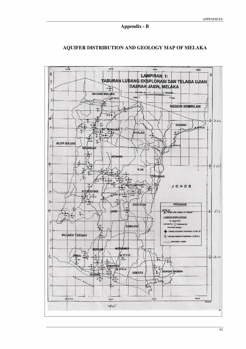
APPENDICES
82
Appendix - B
AQUIFER DISTRIBUTION AND GEOLOGY MAP OF MELAKA

APPENDICES
83

APPENDICES
84

APPENDICES
85

APPENDICES
86

APPENDICES
87
Appendix - C
BOREHOLES DATA OF DEEP AQUIFERS
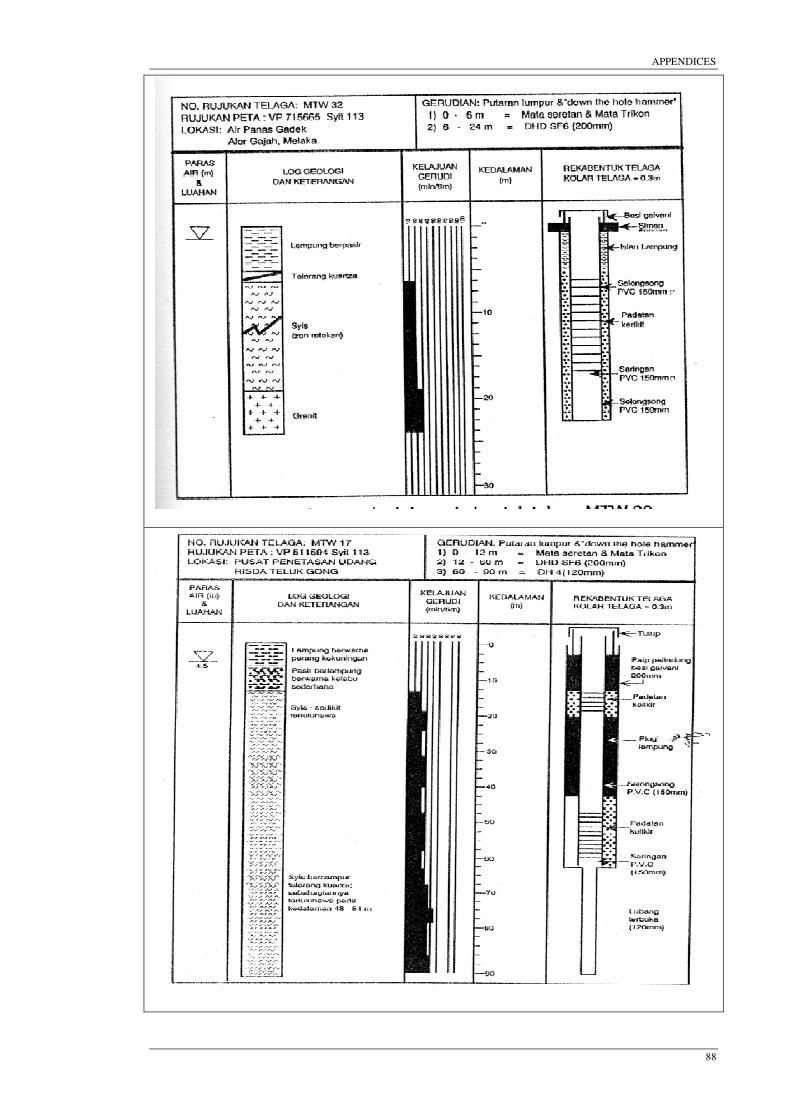
APPENDICES
88

APPENDICES
89

APPENDICES
90

APPENDICES
91

APPENDICES
92

APPENDICES
93
Appendix – D
BOREHOLES DATA OF SHALLOW AQUIFERS

APPENDICES
94

APPENDICES
95
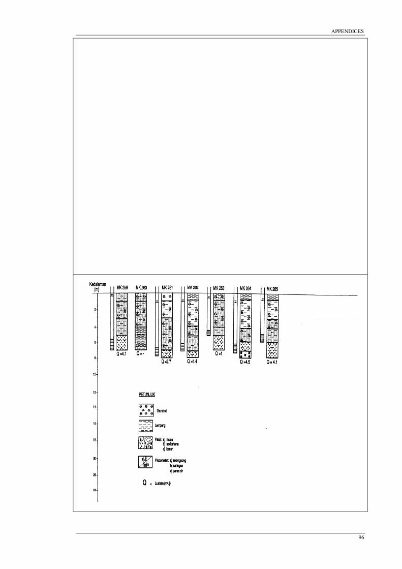
APPENDICES
96

APPENDICES
97

APPENDICES
98

APPENDICES
99

APPENDICES
100

APPENDICES
101
Appendix – E
DRINKING WATER QUALITY STANDARD – MALAYSIA, 1992
Table 1: Drinking Water Quality Standard - Malaysia, 1992
Parameter
Parameter Short
Name Group Raw Water Treated Water
Turbidity NTU
Physical
100 5
Color TCU 300(Hazen) 15
pH pH 5.5-9 6.5-9
Total Dissolved Solids TDS
Inorganic
1500 1000
Chloride Cl 250 250
Ammonia NH4-N 0.5 0.5
Nitrate No3-N 10 10
Iron Fe 1 0.3
Fluoride Fl 1.5 0.9
Total Nitrogen NO3 1 -
Violence 500 500
Manganese Mn
Element Effects
0.2 -
Copper Cu 1 1
Mercury Hg 0.001 0.001
Cadmium Cd 0.005 0.005
Arsenic As 0.05 0.05
Cyanide Cn 0.1 0.1
Lead Pb 0.1 0.05
Chromium Cr 0.05 0.05
Zink Zn 5 5
Sodium Na 200 200
Sulfate SO4 400 400
Selenium Se 0.01 0.01
Silver Ag 0.05 0.05
Magnesium Mg 150 150
Oil Mineral MykMin 0.3 0.3
Phenol C6H5OH 0.002 0.002

APPENDICES
102
Appendix – F
SHALLOW AND DEEP BOREHOLES PROFILE IN MELAKA
Table 1: The Number of Shallow Boreholes in Alor Gajah District
No. Code
Location Depth Discharge Main
Number (m) cu.m/hour Stone
1 MK 1 Kg Lendu 4.00 2.00 Granite
2 MK 2 Kg Pantai Belimbing 4.80 6.00 Phyllite
3 MK 3 Kg Melaka Pindah 3.60 3.50 Schist
4 MK 4 Tabika Kemas, Blimbing Dalam
6.20 2.00 Phyllite
5 MK 5 Kg Air Pasir 6.20 4.00 Granite
6 MK 6 Loji Air Gadek 13.00 11.40 Granite
7 MK 7 Kg Padang Kemunting 8.00 12.30 Granite
8 MK 8 Kg Pulau Sedang 7.50 4.50 Granite
9 MK 9 Kg Air Limau 4.00 1.00 Granite
10 MK 10 Kg Tehel Solok 9.50 2.00 Phyllite
11 MK 11 Kg Pantai Belimbing 6.10 9.00 Phyllite
12 MK 12 Kg Sungai Siput 5.50 12.00 Phyllite
13 MK 13 Kg Berisau 4.30 12.00 Phyllite
14 MK 14 Kg Air Pak Abas 4.50 5.00 Phyllite
15 MK 22 Pulau Sebang 10.00 9.00 Granite
16 MK 23 Ladang Liang Guat 10.00 9.50 Granite
17 MK 24 Kg Dalong 9.00 9.50 Granite
18 MK 25 Ladang Liang Guat 8.50 18.00 Granite
19 MK 26 Pulau Sebang 7.00 8.00 Granite
20 MK 27 Kg Padang Sebang 9.00 11.20 Granite
21 MK 28 Tg Rimau 6.50 3.60 Granite
22 MK 49 Solok Duku 7.00 12.70 Schist
23 MK 50 Solok Duku 6.00 2.00 Schist
24 MK 51 Kg Air Molek 12.50 8.00 Phyllite
25 MK 52 Telok Gong 15.00 4.50 Schist
26 MK 56 Padang Kemunting 4.00 3.00 Granite
27 MK 57 Kg Tengah 20.00 2.70 Schist
28 MK 59 Kg Nelayan Kuala Linggi 25.00 18.00 Granite
29 MK 61 Ladang Liang Guat 7.00 5.50 Granite
30 MK 62 Tanjung Bidara 8.00 0.50 Granite

APPENDICES
103
Table 1: The Number of Shallow Boreholes in Alor Gajah District (continue)
No. Code
Location Depth Discharge Main
Number (m) cu.m/hour Stone
31 MK 63 Pekan Lubak Cina 16.00 6.40 Phyllite
32 MK 64 Solok Air Batu 6.50 0.90 Phyllite
33 MK 65 Solok Mek Selama 2.00 0.00 Granite
34 MK 66 Loji Air Gadek 5.70 0.90 Granite
35 MK 68 Rumah Pam Durian Tunggal 13.00 0.00 Schist
36 MK 69 Rumah Pam Durian Tunggal 8.50 0.00 Granite
37 MK 70 Kg Gadek 7.50 0.00 Granite
38 MK 71 Kg Gadek 10.00 0.00 Granite
39 MK 72 Kg Tanjung Rimau 6.50 0.00 Granite
40 MK 73 Ladang Liang Guat 4.00 0.00 Granite
41 MK 74 Ladang Liang Guat 3.00 0.00 Granite
42 MK 75 Kg Kemuning 4.00 0.00 Granite
43 MK 77 Air Hitam Ulu 6.50 0.00 Granite
44 MK 78 Kg Lodang 3.00 0.00 Schist
45 MK 79 Kg Paya Rumput 4.00 0.00 Schist
46 MK 80 Solok Air Limau Nipis 3.50 0.00 Schist
47 MK 83 Ulu Lendu 3.00 0.00 Schist
48 MK 84 Felda Hutan fercha 8.00 0.60 Granite
49 MK 85 Kg Sungai Petai 4.60 0.00 Phyllite
50 MK 86 Kg Telok Gong 8.00 0.20 Granite
51 MK 87 Kg Solok Ubai 3.10 1.20 Granite
52 MK 88 Kg Sg Jernih 4.20 0.50 Granite
53 MK 89 Pekan Rembia 5.20 2.50 Phyllite
54 MK 90 Kg Tengah, Durian Tunggal 8.00 0.00 Schist
55 MK 119 Kampung Tanjung Dahan 18.00 0.00 Granite
56 MK 120 Kampung Tanjung Dahan 11.00 4.50 Schist
57 MK 138 Sg Buloh 4.00 1.00 Granite
58 MK 139 Kg Durian Daun 3.00 0.00 Phyllite
59 MK 150 Pasir Gempor 11.00 0.50 Granite
60 MK 152 Solok Mangga 7.00 0.00 Granite

APPENDICES
104
Table 1: The Number of Shallow Boreholes in Alor Gajah District (continue)
No. Code
Location Depth Discharge Main
Number (m) cu.m/hour Stone
61 MK 153 Solok Mangga 18.00 2.70 Granite
62 MK 154 Padang Kemunting 5.00 14.00 Granite
63 MK 155 Kg Hailan 6.00 8.00 Granite
64 MK 156 Jalan Kolam Air 10.00 12.00 Granite
65 MK 197 Pengkalan Balak 14.00 2.50 Granite
66 MK 198 Kuala Sg Baru 11.00 0.00 Schist
67 MK 199 Kg Telok Belanga 3.00 0.50 Granite
68 MK 200 Kg Telok Gong 13.00 1.40 Granite
69 MK 201 Sungai Tuang 14.00 0.50 Phyllite
70 MK 219 Kampung Pancor 3.00 0.00 Phyllite
71 MK 220 Masjid Durian Tunggal 6.00 0.50 Phyllite
72 MK 227 Kg Air Manggis 4.00 0.00 Granite
73 MK 232 Kg Paya Rumput 6.00 0.50 Granite
Table 2: The Number of Deep Boreholes in Alor Gajah District
No. Code
Location Depth Discharge Main
Number (m) cu.m/hour Stone
1 Pusat pertaian Sungai Udang 113 6 Phyllite/ Schist
2 Ladang sg. Baru, Mukim Masjid tanah 76 0 Phyllite
3 Ladang pegoh, Mukim Pengoh 68 9 Phyllite
4 Ladang Bertam, Mkm Durian Tunggal 76 6 Phyllite
5 Ladang Home, Mkm Kuala Sg Baru 77 8 Quartz
6 Kilang Sinma, Sg Baru Ilir 200 5 Schist
7 MARDEC Durian, Mkm Durian Tunggal
900 10 Phyllite

APPENDICES
105
Table 3: The Number of Shallow Boreholes in Melaka Tengah District
No. Code
Location Depth Discharge Main
Number (m) cu.m/hour Stone
1 MK 53 Kg Paya Rumput Jaya, Sg Udang
4.00 0.60 Granite
2 MK 54 Kg Paya Rumput Jaya, Sg Udang
5.00 8.20 Granite
3 MK 55 Kg Paya Rumput Jaya, Sg Udang
7.00 0.60 Granite
4 MK 60 Pusat Latihan Pertanian, Sg Udang
6.00 7.70 Granite
5 MK 67 Balai Polis Bandar Hilir 4.00 0.00 Schist
6 MK 81 Kelab Melaka, Tanjong Keling 4.00 0.00 Schist
7 MK 82 Kelab Melaka, Tanjong Keling 14.00 0.00 Schist
8 MK 91 Pusat Pertanian, Pulau Gadong 12.00 0.00 Metasediment
9 MK 92 Sekolah Munshi Abdullah, Air Keroh
2.80 0.00 Metasediment
10 MK 93 Kg Bt Baru Dalam 17.00 0.00 Metasediment
11 MK 111 Tangga Batu 5.25 0.00 Metasediment
12 MK 112 Tangga Batu 4.50 0.00 Metasediment
13 MK 113 Kg Tanah Merah 6.00 0.00 Metasediment
14 MK 114 Kg Tanah Merah 8.00 0.00 Metasediment
15 MK 115 Kg Tanah Merah 6.00 0.00 Metasediment
16 MK 116 Kg Batu Punggung, Pantai Kundur
10.00 0.00 Metasediment
17 MK 117 Pantai Tanah Merah, Pantai Kundur
14.00 0.00 Metasediment
18 MK 118 Kg Tambak Paya, Air Keroh 15.50 0.00 Metasediment
19 MK 121 Kg Paya Redan, Tiang Dua 10.00 0.70 Metasediment
20 MK 122 Kg Bukit Nibong, Tiang Dua 12.00 0.00 Metasediment
21 MK 123 Solok Hj. Madzuki, Bukit Lintang
3.25 0.00 Metasediment
22 MK 124 Pulau Gadong 2.00 0.00 Metasediment
23 MK 125 Kg Bertam Malim 2.00 0.00 Metasediment
24 MK 126 Permatang Kelebang 19.00 1.00 Metasediment
25 MK 127 Taman Bukit Rambai 4.25 0.00 Metasediment
26 MK 128 Surau sg Udang 3.50 0.00 Metasediment
27 MK 129 Kg Bukit Beruang 5.25 0.00 Metasediment
28 MK 141 Pantai Kundur 5.00 0.00 Schist

APPENDICES
106
Table 3: The Number of Shallow Boreholes in Melaka Tengah District (continue)
No. Code
Location Depth Discharge Main
Number (m) cu.m/hour Stone
31 MK 144 Bt 10, Kg Pantai Kundor 7.00 0.00 Schist
32 MK 145 Pantai Rombang 9.00 0.00 Schist
33 MK 146 Pantai Rombang 4.00 0.00 Schist
34 MK 147 Kg Pantai Kundor 8.50 0.50 Schist
35 MK 148 Pengkalan Perigi 5.00 0.00 Schist
36 MK 149 Pengkalan Perigi 4.00 0.00 Schist
37 MK 157 Sek Men Tun Tuah Bachang
10.50 0.00 Metasediment
38 MK 158 Kg Pantai Tanah Merah 9.00 1.00 Granite
39 MK 159 Kg Pantai Tanah Merah 9.00 1.00 Granite
40 MK 160 Masjid Jamek Kg Pernu 8.00 2.00 Metasediment
41 MK 98 Pengkalan Badak 15.00 0.00 Granite
42 MK 183 Pengkalan Rama 7.00 0.00 Metasediment
43 MK 184 Kg Pantai Rombang 9.00 1.50 Schist
44 MK 185 Kg Pantai Rombang 6.00 0.00 Schist
45 MK 186 Kg Pantai Rombang 8.00 2.00 Schist
46 MK 187 Kg Sg Lereh 11.00 0.50 Schist
47 MK 190 Kg Tanjung Keling 6.00 0.00 Metasediment
48 MK 191 Tanjung Keling 7.50 8.00 Metasediment
49 MK 192 Sg Lerek, Tg Keling 14.00 0.00 Metasediment
50 MK 196 Kg Nelayan Tg Keling 4.00 2.00 Metasediment
51 MK 202 Kg Telok Mas 8.00 0.00 Metasediment
52 MK 203 Kg Telok Mas 14.00 0.00 Metasediment
53 MK 204 Kg Ketapang Pernu 7.50 13.50 Metasediment
54 MK 205 Kg Solok Tengkera 9.50 2.50 Metasediment
55 MK 206 Jalan Tengkera 10.00 1.00 Metasediment
56 MK 207 Kg Ujong Pasir 8.00 0.00 Metasediment
57 MK 208 Pulau Dodol 2.50 0.00 Granite
58 MK 209 Pulau Dodol 2.00 0.00 Granite
59 MK 210 Kg Bukit Cina 5.00 0.00 Metasediment
60 MK 211 Padang Temu, Sg Duyong 14.00 0.00 Metasediment
61 MK 212 Masjid Bt Lima, Kandang 14.00 0.00 Metasediment
62 MK 216 Jalan Tanjung Minyak, Rembia
10.00 0.00 Metasediment

APPENDICES
107
Table 3: The Number of Shallow Boreholes in Melaka Tengah District (continue)
No. Code
Location Depth Discharge Main
Number (m) cu.m/hour Stone
64 MK 225 Bukit Rambai 10.00 0.00 Metasediment
65 MK 226 Tanjong Minyak 6.00 0.50 Metasediment
66 MK 233 Kem Terendak, Sg Udang 10.00 2.00 Granite
67 MK 234 Kem Terendak, Sg Udang 11.00 1.00 Granite
68 MK 235 Kem Terendak, Sg Udang 7.00 0.00 Granite
69 MK 236 Kem Terendak 10.00 1.00 Granite
70 MK 237 Kem Terendak 13.00 4.50 Granite
71 MK 238 Kem Terendak 10.00 0.50 Granite
72 MK 239 Kem Terendak 6.00 4.00 Granite
73 MK 240 Kem Terendak 6.00 1.00 Granite
74 MK 241 Kem Terendak 10.00 1.00 Granite
75 MK 242 Kem Terendak 10.00 4.50 Granite
76 MK 243 Kem Terendak 10.00 2.00 Granite
77 MK 244 Kem Terendak 10.00 7.00 Granite
78 MK 245 Kg Baru Pantai Kundor 8.00 1.00 Schist
79 MK 246 Kem Terendak 8.00 4.50 Granite
80 MK 247 Kem Terendak 8.00 2.00 Granite
81 MK 248 Kem Terendak 6.00 4.00 Granite
82 MK 249 Kem Terendak 8.00 3.50 Granite
83 MK 250 Kem Terendak 7.00 0.00 Granite
84 MK 251 Kem Terendak 3.00 0.00 Granite
85 MK 252 Kem Terendak 7.50 4.00 Granite
86 MK 253 Kem Terendak 7.50 5.50 Granite
87 MK 254 Kem Terendak 6.00 0.00 Granite
88 MK 255 Kem Terendak 7.50 2.00 Granite
89 MK 256 Kem Terendak 8.00 2.00 Granite
90 MK 257 Kem Terendak 6.50 0.00 Granite
91 MK 258 Kem Terendak 7.00 4.00 Granite
92 MK 259 Kem Terendak 9.00 8.00 Granite
93 MK 260 Kem Terendak 6.50 0.00 Granite

APPENDICES
108
Table 3: The Number of Shallow Boreholes in Melaka Tengah District (continue)
No. Code
Location Depth Discharge Main
Number (m) cu.m/hour Stone
94 MK 261 Kem Terendak 7.50 2.50 Granite
95 MK 262 Kem Terendak 8.00 1.50 Granite
96 MK 263 Kem Terendak 6.50 1.00 Granite
97 MK 264 Kem Terendak 7.50 4.50 Granite
98 MK 265 Kem Terendak 7.50 4.00 Granite
99 MK 106 Parit Perawas Sg Rambai 15.50 0.00 Schist
100 MK 107 Kg Cap Tangan 12.50 0.00 Schist
101 MK 108 Parit Penghulu Benting 14.00 0.00 Schist
102 MK 109 Kg Tasik Teluk Gong 19.50 0.00 Schist
Table 4: The Number of Deep Boreholes in Melaka Tengah District
No. Code
Location Depth Discharge Main
Number (m) cu.m/hour Stone
1 - Ladang Getah Lee, kerubong
75.00 5.00 Schist
2 - Taman Aggrerik, kelebang 20.00 5.00 Aluvium
3 - Hospital Besar Melaka 20.00 5.00 Schist
4 - Klinik Bukit Baru 30.00 4.00 Schist
5 - Kilang Kertas Seng Kong 100 18 Schist

APPENDICES
109
Table 5: The Number of Shallow Boreholes in Jasin District
No. Code
Location Depth Discharge Main
Number (m) cu.m/hour Stone
1 MK 10 Solok Tehel 9.50 2.00 Shale
2 MK 15 Pekan tehel 13.00 2.70 Shale
3 MK 16 Ulu Jasin 4.50 2.50 Shale
4 MK 17 Batu 21 jalan Selandar 6.00 16.00 Shale
5 MK 18 Batu 24 Ja;an Selandar 9.00 2.20 Shale
6 MK 19 Bukit Senggeh 5.00 18.50 Schist
7 MK 20 Anak Air keroh, Selandar 5.00 9.00 Schist
8 MK 21 Kg Tengah, Selandar 6.00 7.00 Schist
9 MK 29 Pulau selendar 7.00 1.00 Schist
10 MK 30 Pekan Jasin 8.50 12.30 Schist
11 MK 31 Lubok Kesau, Benban 11.50 5.50 Schist
12 MK 32 Kesang pajak 9.00 10.70 Schist
13 MK 33 Solok Pondok, Keempas 7.50 7.70 Schist
14 MK 34 Kesang Tua 8.00 5.50 Schist
15 MK 35 Sek Iskandar Syah 8.00 2.00 Schist
16 MK 36 Kg Kelubi 7.00 9.60 Schist
17 MK 37 Solok Gapam 8.00 5.50 Granite
18 MK 38 Km 14. Jln Jasin Bemban 9.50 0.70 Schist
19 MK 39 Km 7, Jasin Nyala 5.00 10.00 Schist
20 MK 40 Kg Rim 8.80 8.20 Schist
21 MK 41 Gong Bangkong 10.00 5.50 Schist
22 MK 42 Kg Tengah, Btg Melaka 4.00 4.00 Schist
23 MK 43 Solok Ulu Gapis 5.00 7.30 Schist
24 MK 44 Tedong Darat 8.00 10.30 Schist
25 MK 45 Tedong Darat 8.50 4.10 Schist
26 MK 46 Paya Rayong 12.50 2.00 Schist
27 MK 47 Seberang darat, Merlimau 12.00 2.00 Schist
28 MK 48 Ulu Jasin 5.50 3.30 Schist
29 MK 58 Serkam darat 15.00 2.30 Schist
30 MK 94 Solok Serompong 3.00 0.00 Granite

APPENDICES
110
Table 5: The Number of Shallow Boreholes in Jasin District (continue)
No. Code
Location Depth Discharge Main
Number (m) cu.m/hour Stone
31 MK 95 Ulu Duyung 4.50 0.00 Schist
32 MK 96 Selandar 5.00 0.00 Schist
33 MK 97 Paya Kundang 15.00 0.00 Granite
34 MK 99 Bukit Kajang 2.25 0.00 Granite
35 MK 100 Air Panas 2.25 0.00 Granite
36 MK 101 Cabau 7.00 0.00 Granite
37 MK 102 Asahan 4.50 0.00 Granite
38 MK 104 Paya Tanjung 7.00 0.00 Granite
39 MK 106 Parit Perawas 15.50 0.00 Laterite
40 MK 108 Parit Penghulu 14.00 0.00 Laterite
41 MK 109 Telok Gong 19.50 0.00 Schist
42 MK 110 Air Kangkong 110.00 0.00 Granite
43 MK 130 Kesang 11.00 0.00 Laterite
44 MK 133 Batu 21 Kesang 8.00 0.00 Laterite
45 MK 134 Heifer's Park 4.00 0.00 Laterite
46 MK 135 Batu 15 Merlimau 9.00 1.80 Granite
47 MK 136 Batu Melaka 4.00 0.00 Laterite
48 MK 161 Solok Pasal 10.00 0.00 Schist
49 MK 178 Kg Kumpai, Cenderah 14.00 4.00 Granite
50 MK 179 Kg Nelayan, Tg Keling 4.00 0.00 Schist
51 MK 180 Air Molek 14.00 1.40 Schist
52 MK 181 Solok Minyak barat 10.00 3.00 Schist
53 MK 193 Permatang Pasir 10.00 0.50 Schist
54 MK 76 Kg Tengah, Selandar 6.00 0.00 Schist
55 MK 213 Simpang Jasin_Bemban 6.00 0.00 Granite
56 MK 214 Air Barok 10.00 3.60 Granite
57 MK 215 Felda kemendor 8.00 1.00 Granite
58 MK 221 Felda Lembah Kesang 9.00 2.00 Granite
59 MK 223 Surau Cincin 3.50 0.00 Granite
60 MK 224 Simpang Kumpai 11.00 13.60 Granite
61 MK 229 Simpang Cincin/Tangkak 6.00 0.00 Granite
62 MK 230 Risda Sg Duyung 6.00 0.50 Granite
63 MK 231 Blai Islam 9.00 0.50 Granite
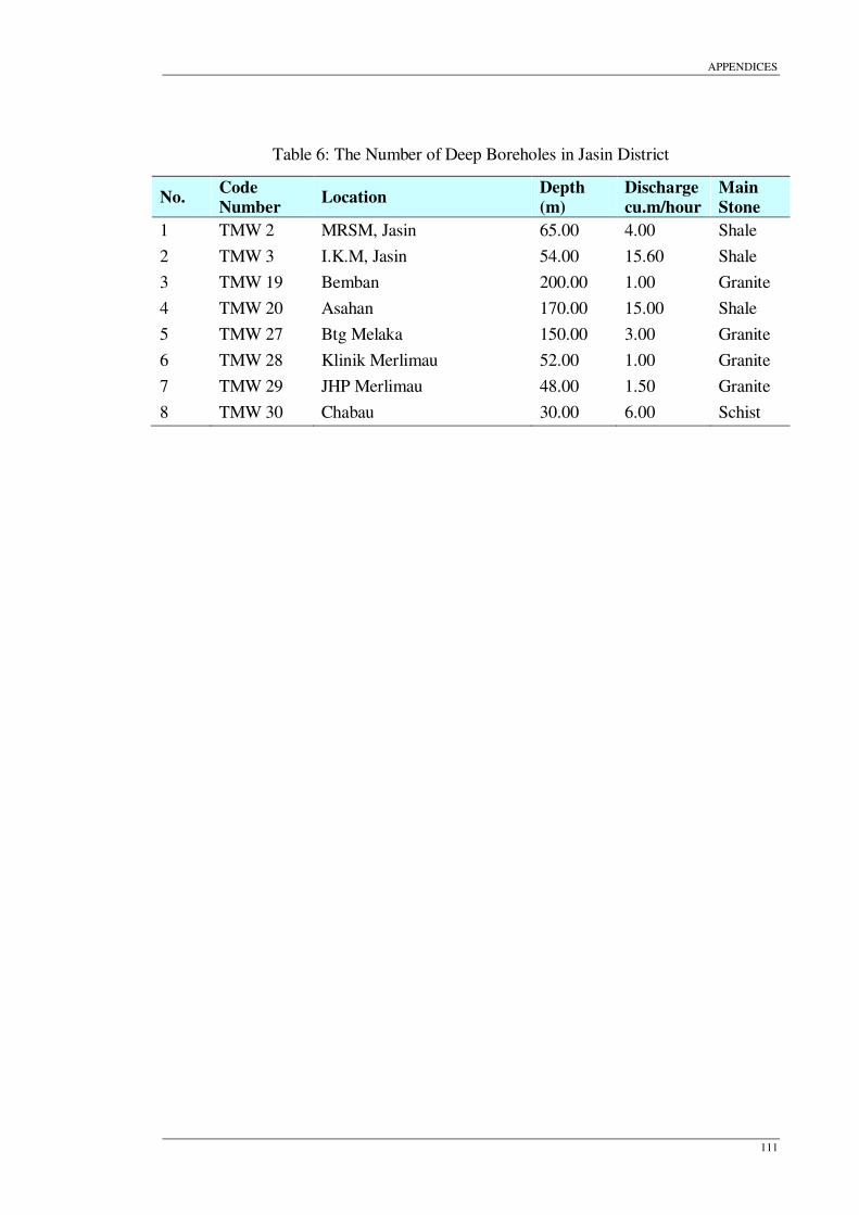
APPENDICES
111
Table 6: The Number of Deep Boreholes in Jasin District
No. Code
Location Depth Discharge Main
Number (m) cu.m/hour Stone
1 TMW 2 MRSM, Jasin 65.00 4.00 Shale
2 TMW 3 I.K.M, Jasin 54.00 15.60 Shale
3 TMW 19 Bemban 200.00 1.00 Granite
4 TMW 20 Asahan 170.00 15.00 Shale
5 TMW 27 Btg Melaka 150.00 3.00 Granite
6 TMW 28 Klinik Merlimau 52.00 1.00 Granite
7 TMW 29 JHP Merlimau 48.00 1.50 Granite
8 TMW 30 Chabau 30.00 6.00 Schist

APPENDICES
112
Appendix – G
GROUNDWATER QUALITY DATA OF MELAKA
Table 1: Water Quality Data in Shallow Boreholes – Alor Gajah District
Parameters MK-120 KSB-Ib) MK-52 MK-57 MK-200
Turbidity 3.5 0.9 0.9 150 38 Color 5 5 5 5 5 pH 8 5.2 7.4 7 3.7 TDS 6760 1936 222 2456 1038 Chloride (Cl) 3230 2220 40 980 16 Ammonia (NH4-N) 1.8 0.65 0.88 0.06 0.08 Nitrate (NO3-N) 9 96 12 <3 <3 Iron (Fe) 16.9 2.6 8.5 <0.1 6 Fluoride (F) <0.5 4.1 <0.5 <0.5 <0.5 Arsenic (As) <0.005 0.006 <0.005 <0.005 0.007 Copper <0.1 <0.1 <0.1 <0.1 <0.1 Magnesium (Mg) 232 116 9.9 62 1.1 Manganese (Mn) 8.3 2.4 <0.1 <0.1 0.4 Zink (Zn) <0.1 <0.1 0.1 <0.1 0.4 Sodium (Na) 1480 1015 37 575 11 Sulfate(So4) 450 210 70 73 28 Calcium(Ca) 220 147 4.2 36 4.6 Bicarbonate(Hco3) 127 23 35 260 <1 Silica(Si) 13 13 16 14 5.1 Carbonate(Co3) 5 <1 <1 3 <1 Aluminum(Al) 0.1 0.2 <0.1 <0.1 0.3 Potassium(K) 88 38 4.2 35 1.7 Cadmium(Cd) <0.1 <0.01 <0.1 <0.1 <0.01 Phosphorus(P) <0.02 0 <0.02 <0.02 0.03 Conductivity 10,200 2850 310 3670 144 Sodium nibs 16.61 15.2 2.25 13.47 1.20
Note: all parameter as concentration (mg/l), exclude pH, Turbidity and Conductivity

APPENDICES
113
Table 1: Water Quality Data in Shallow Boreholes – Alor Gajah District (continue)
Parameters MK-51 MK-12 MK-14 MK-7 MK-56
Turbidity 0.9 135 30 11 0 Color 5 5 5 5 5 pH 8 7.6 5.9 5 6.6 TDS 852 416 92 94 76 Chloride (Cl) 385 27 6 14 6 Ammonia (NH4-N) 0.72 0.02 0.02 0.06 0.02 Nitrate (NO3-N) 4 <3 <13 <3 <3 Iron (Fe) 8.8 2.4 0.4 2.1 0.1 Fluoride (F) <0.5 <0.5 <0.5 <0.5 <0.5 Arsenic (As) <0.005 <0.005 <0.005 <0.005 <0.005 Copper <0.1 <0.1 <0.1 <0.1 <0.1 Magnesium (Mg) 15 3.6 0.8 0.5 0.5 Manganese (Mn) 0.2 0.3 <0.1 <0.1 <0.1 Zink (Zn) 0.4 <0.1 0.1 <0.1 <0.1 Sodium (Na) 272 28 7.5 13 6.2 Sulfate(So4) 125 <5 <5 15 31 Calcium(Ca) 21 5 1.3 1.7 0.8 Bicarbonate(Hco3) 93 62 1 <1 <1 Silica(Si) 14 28 18 5.3 21 Carbonate(Co3) 4 <1 <1 <1 <1 Aluminum(Al) <0.1 <0.1 <0.1 <0.1 <0.1 Potassium(K) 10 10 1.3 3.5 <0.5 Cadmium(Cd) <0.1 <0.1 <0.1 <0.1 <0.1 Phosphorus(P) <0.02 <0.02 0.02 <0.02 <0.02 Conductivity 1,504 210 56 108 171 Sodium nibs 11.08 2.33 1.28 2.25 1.30
Note: all parameter as concentration (mg/l), exclude pH, Turbidity and Conductivity

APPENDICES
114
Table 1: Water Quality Data in Shallow Boreholes – Alor Gajah District (continue)
Parameters MK-154 MK-155 MK-197 MK-8 MK-22
Turbidity 9 14 24 185 148 Color 5 70 5 5 5 pH 4.5 6.8 5.6 6.6 6.5 TDS 128 104 306 328 164 Chloride (Cl) 17 13 7 12 8 Ammonia (NH4-N) 0.4 0.64 0.02 0.24 0.24 Nitrate (NO3-N) <3 3 <3 <3 3 Iron (Fe) 4.4 1.9 1.3 16.2 2.4 Fluoride (F) <0.5 <0.5 <0.5 <0.5 <0.5 Arsenic (As) <0.005 <0.005 <0.005 <0.005 <0.005 Copper <0.1 <0.1 <0.1 <0.1 <0.1 Magnesium (Mg) 1.3 1.8 0.8 2.1 3.9 Manganese (Mn) <0.1 <0.1 0.2 0.3 0.5 Zink (Zn) <0.1 <0.1 <0.1 <0.1 0.2 Sodium (Na) 19 10 5.3 14 14 Sulfate(So4) 35 15 <3 <0.5 <0.5 Calcium(Ca) 7.8 2.2 2.2 16 7.8 Bicarbonate(Hco3) 10 10 20 66 68 Silica(Si) 3.2 5.3 15 21 21 Carbonate(Co3) <1 <1 <1 <1 <1 Aluminum(Al) 0.1 0.6 <0.1 <1 0.2 Potassium(K) 4.3 8.6 2.7 3.5 5.1 Cadmium(Cd) <0.1 <0.1 <0.01 <0.1 <0.1 Phosphorus(P) 0.05 0.05 0.18 0.05 0.02 Conductivity 161 117 56 177 144 Sodium nibs 161 1.21 0.78 0.87 1.02
Note: all parameter as concentration (mg/l), exclude pH, Turbidity and Conductivity
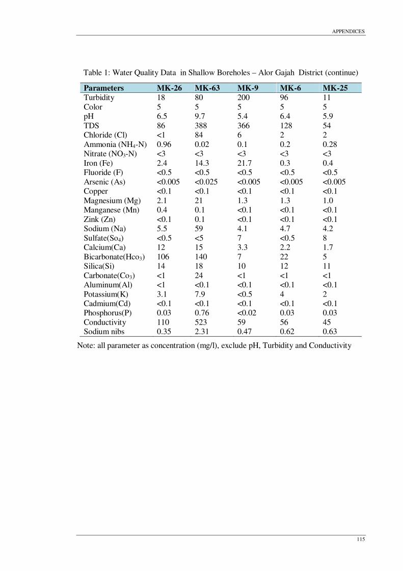
APPENDICES
115
Table 1: Water Quality Data in Shallow Boreholes – Alor Gajah District (continue)
Parameters MK-26 MK-63 MK-9 MK-6 MK-25
Turbidity 18 80 200 96 11 Color 5 5 5 5 5 pH 6.5 9.7 5.4 6.4 5.9 TDS 86 388 366 128 54 Chloride (Cl) <1 84 6 2 2 Ammonia (NH4-N) 0.96 0.02 0.1 0.2 0.28 Nitrate (NO3-N) <3 <3 <3 <3 <3 Iron (Fe) 2.4 14.3 21.7 0.3 0.4 Fluoride (F) <0.5 <0.5 <0.5 <0.5 <0.5 Arsenic (As) <0.005 <0.025 <0.005 <0.005 <0.005 Copper <0.1 <0.1 <0.1 <0.1 <0.1 Magnesium (Mg) 2.1 21 1.3 1.3 1.0 Manganese (Mn) 0.4 0.1 <0.1 <0.1 <0.1 Zink (Zn) <0.1 0.1 <0.1 <0.1 <0.1 Sodium (Na) 5.5 59 4.1 4.7 4.2 Sulfate(So4) <0.5 <5 7 <0.5 8 Calcium(Ca) 12 15 3.3 2.2 1.7 Bicarbonate(Hco3) 106 140 7 22 5 Silica(Si) 14 18 10 12 11 Carbonate(Co3) <1 24 <1 <1 <1 Aluminum(Al) <1 <0.1 <0.1 <0.1 <0.1 Potassium(K) 3.1 7.9 <0.5 4 2 Cadmium(Cd) <0.1 <0.1 <0.1 <0.1 <0.1 Phosphorus(P) 0.03 0.76 <0.02 0.03 0.03 Conductivity 110 523 59 56 45 Sodium nibs 0.35 2.31 0.47 0.62 0.63
Note: all parameter as concentration (mg/l), exclude pH, Turbidity and Conductivity

APPENDICES
116
Table 1: Water Quality Data in Shallow Boreholes – Alor Gajah District (continue)
Parameters MK-156 MK-72 MK-23 MK-24 MK-5
Turbidity 155 22 52 2.7 30 Color 5 5 5 5 5 pH 8.0 5.2 6.5 5.8 7.4 TDS 132 254 140 36 240 Chloride (Cl) 3 6 <1 <1 1 Ammonia (NH4-N) 1.4 0.04 0.44 0.32 0.02 Nitrate (NO3-N) <3 <1 <3 <3 <0.3 Iron (Fe) 17 0.1 0.7 2.6 11.1 Fluoride (F) 1 <0.5 <0.5 <0.5 <0.5 Arsenic (As) <0.005 0.017 <0.005 <0.005 <0.005 Copper <0.1 <0.1 <0.1 <0.1 <0.1 Magnesium (Mg) 1.3 0.3 2.4 0.8 1.8 Manganese (Mn) 0.3 <0.3 0.2 <0.1 0.1 Zink (Zn) <0.1 <0.1 <0.1 <0.1 <0.1 Sodium (Na) 15 62 10 1.4 7.7 Sulfate(So4) <5 7 <0.5 <0.5 <5 Calcium(Ca) 13 4.1 12 1.7 13 Bicarbonate(Hco3) 90 150 76 10 67 Silica(Si) 23 53 28 11 31 Carbonate(Co3) <1 6 <1 <1 <1 Aluminum(Al) <0.1 <0.1 <0.1 <0.1 <0.1 Potassium(K) 3.5 3.3 1.6 0.3 3.4 Cadmium(Cd) <0.1 <0.01 <0.1 <0.1 <0.1 Phosphorus(P) 0.03 14 0.03 0.02 0.77 Conductivity 138 311 124 26 129 Sodium nibs 1.06 8.11 0.69 0.22 0.55
Note: all parameter as concentration (mg/l), exclude pH, Turbidity and Conductivity

APPENDICES
117
Table 1: Water Quality Data in Shallow Boreholes – Alor Gajah District (continue)
Parameters MK-2 MK-3 MK-4 MK-49 MK-50
Turbidity 95 45 110 1.3 1.3 Color 5 5 5 5 5 pH 6.5 5.9 4 7.9 7.9 TDS 322 278 214 114 188 Chloride (Cl) 2 14 17 1 <1 Ammonia (NH4-N) 0.16 0.06 0.04 0.24 0.04 Nitrate (NO3-N) <3 4 8 4 4 Iron (Fe) 13.5 1.7 9.9 8.7 0.6 Fluoride (F) <0.5 <0.5 <0.5 <0.5 <0.5 Arsenic (As) <0.005 <0.005 <0.005 <0.005 <0.005 Copper <0.1 <0.1 <0.1 <0.1 <0.1 Magnesium (Mg) 19 0.8 <0.5 3.6 2.3 Manganese (Mn) 1.2 0.2 <0.1 0.2 <0.1 Zink (Zn) <0.1 <0.1 <0.1 <0.1 <0.1 Sodium (Na) 8.6 10 12 7.2 11 Sulfate(So4) 73 9 6 <5 <5 Calcium(Ca) 15 2.5 1.7 16 8 Bicarbonate(Hco3) 54 11 <1 76 61 Silica(Si) 38 21 10 42 68 Carbonate(Co3) <1 <1 <1 6 4 Aluminum(Al) <0.1 <0.1 <0.1 <0.1 <0.1 Potassium(K) 2 5.8 2.3 2.5 5.3 Cadmium(Cd) <0.1 <0.1 <0.1 <0.1 <0.1 Phosphorus(P) <0.02 <0.02 <0.02 <0.02 <0.02 Conductivity 281 97 152 120 111 Sodium nibs 0.36 1.41 2.15 0.41 0.88
Note: all parameter as concentration (mg/l), exclude pH, Turbidity and Conductivity

APPENDICES
118
Table 2: Water Quality Data in Deep Boreholes – Alor Gajah District
Parameters MTW-15 MTW-4 MTW-18 MTW-31 MTW-21
Turbidity 8.1 11 10 9.2 0.9
Color 5 5 5 5 5
pH 5.2 5.2 5.2 5.2 5.2
TDS 2720 54 80 28 196
Chloride (Cl) 1095 2 2 1 7
Ammonia (NH4-N) 0.08 0.28 <0.02 0.08 196
Nitrate (NO3-N) 9 <3 4 <3 7
Iron (Fe) 4.1 0.4 0.3 3.1 <0.02
Fluoride (F) 0.8 <0.5 <0.5 <0.5 5
Arsenic (As) 0.021 <0.005 <0.005 <0.005 1.3
Copper <0.1 <0.1 <0.1 <0.1 <0.5
Magnesium (Mg) 81 1.0 3.6 1.4 <0.005
Manganese (Mn) 1.9 <0.1 0.3 <0.5 <0.1
Zink (Zn) <0.1 <0.1 <0.1 <0.1 3.4
Sodium (Na) 445 4.2 2.5 6.7 0.3
Sulfate(So4) 204 8 4 7 4
Calcium(Ca) 200 1.7 1.3 0.2 15
Bicarbonate(Hco3) 49 5 5 5 <3
Silica(Si) 26 11 <0.1 11 16
Carbonate(Co3) 0.9 <1 <1 <1 78
Aluminum(Al) 0.2 <0.1 <0.1 <0.1 52
Potassium(K) 12 2 0.8 0.7 <1
Cadmium(Cd) <0.01 <0.1 <0.01 <0.01 0.1
Phosphorus(P) <0.02 0.03 <0.02 0 <0.01
Conductivity 3,700 45 55 31 <162
Sodium nibs 6.71 0.63 0.2 1.17 0.89
Note: all parameter as concentration (mg/l), exclude pH, Turbidity and Conductivity

APPENDICES
119
Table 3: Water Quality Data in Shallow Boreholes – Melaka Tengah District
Parameters MK-143 MK-192 MK- 241 MK-254 MK-126
Turbidity 36 31 5.6 4.3 7450 Color 5 4 5 5 5 pH 7 6.8 4.6 6.9 3.5 TDS 64 756 90 76 4732 Chloride (Cl) 7 90 10 5 <0.005 Ammonia (NH4-N) 0.08 0.02 0.02 0.02 0.1 Nitrate (NO3-N) 4 <3 7 <3 0.12 Iron (Fe) 7.9 5.3 7.9 <0.1 116.5 Fluoride (F) <0.5 <0.5 <0.5 <0.5 4.1 Arsenic (As) <0.005 <0.005 <0.005 <0.005 <0.1 Copper 0.5 <0.1 <0.1 <0.1 <0.1 Magnesium (Mg) 0.5 14 0.6 0.5 <0.02 Manganese (Mn) 0.1 0.3 <0.1 <0.1 0.2 Zink (Zn) <0.1 <0.1 <0.1 <0.1 176 Sodium (Na) 5.2 70 7.5 4.5 128 Sulfate(So4) 45 90 <5 <5 1080 Calcium(Ca) 1.7 31 1.6 1.6 25 Bicarbonate(Hco3) 5 1.18 5 20 <1 Silica(Si) 4.3 22 9.6 17 <1 Carbonate(Co3) <1 <1 <1 <1 2410 Aluminum(Al) 0.4 <0.1 <0.1 <0.1 200 Potassium(K) 4 19 3.3 3.5 4 Cadmium(Cd) <0.01 <0.01 <0.01 <0.01 <0.5 Phosphorus(P) <0.5 <0.5 <0.5 <0.5 4.2 Conductivity 56 665 68 44 15.1 Sodium nibs 4.9 14.7 7.1 4.3 5
Note: all parameter as concentration (mg/l), exclude pH, Turbidity and Conductivity

APPENDICES
120
Table 3: Water Quality Data in Shallow Boreholes – Melaka Tengah District (continue)
Parameters MK-126 MK-205 MK-202
Turbidity 3.5 14 41 Color 5 70 5 pH 4.2 6.8 7.1 TDS 4732 104 284 Chloride (Cl) 2410 13 5 Ammonia (NH4-N) 0.12 0.64 0.2 Nitrate (NO3-N) 4 3 <3 Iron (Fe) 116.5 1.9 1.1 Fluoride (F) <0.5 <0.5 <0.5 Arsenic (As) <0.005 <0.005 <0.005 Copper <0.1 <0.1 <0.1 Magnesium (Mg) 128 1.8 2 Manganese (Mn) 4.1 0.1 0.1 Zink (Zn) 0.2 <0.1 <0.1 Sodium (Na) 1080 10 11 Sulfate(So4) 200 14 9 Calcium(Ca) 176 2.2 2.4 Bicarbonate(Hco3) <1 10 35 Silica(Si) - - - Carbonate(Co3) <1 <1 <1 Aluminum(Al) 0.1 0.6 <1 Potassium(K) 25 8.6 2.2 Cadmium(Cd) <0.5 <0.5 <0.5 Phosphorus(P) 0.02 0.05 0.02 Conductivity 7450 117 78 Sodium nibs 15.1 1.2 1.27
Note: all parameter as concentration (mg/l), exclude pH, Turbidity and Conductivity

APPENDICES
121
Table 4: Water Quality Data in Deep Boreholes – Melaka Tengah District
Parameters MTW-14 MTW-25 MTW-12 MTW-9 MTW-10
Turbidity 8.1 <1 50 33 14
Color 5 5 5 5 5
pH 8.2 8.4 6.7 5.2 8
TDS 268 240 26040 32 242
Chloride (Cl) 0.7 3 13250 6 3
Ammonia (NH4-N) <0.04 0.08 1.1 0.2 0.02
Nitrate (NO3-N) 7 <3 100 <3 <3
Iron (Fe) 1 1 12 0.4 3.5
Fluoride (F) <0.5 <0.5 - <0.5 <0.5
Arsenic (As) <0.005 <0.005 <0.05 <0.005 <0.005
Copper <0.1 <0.1 <0.1 <0.1 <0.1
Magnesium (Mg) 5.7 23 859 0.4 7.6
Manganese (Mn) 0.2 0.1 <0.1 0.1 0.2
Zink (Zn) <0.1 <0.1 <0.1 <0.1 0.2
Sodium (Na) 12 <3 6700 4.1 11
Sulfate(So4) 12 <3 1690 <3 10
Calcium(Ca) 62 30 323 0.4 35
Bicarbonate(Hco3) 188 226 110 11 153
Silica(Si) 1 3 4.9 14 18
Carbonate(Co3) 5 <1 <1 <1 10
Aluminum(Al) 0.7 1 <0.2 <0.01 0.1
Potassium(K) 1 1 235 1.8 6.5
Cadmium(Cd) 8.2 8.4 <0.01 <0.01 <0.01
Phosphorus(P) 0.02 0.02 <0.5 <0.02 0.05
Conductivity 145 333 388000 38 274
Note: all parameter as concentration (mg/l), exclude pH, Turbidity and Conductivity

APPENDICES
122
Table 5: Water Quality Data in Shallow Boreholes – Jasin District
Parameters MK-19 MK-20 MK-30 MK-31 MK-32
Turbidity 5.7 4.7 37 18 27 Color 5 5 5 5 5 pH 7 8.2 7 5.9 7.9 TDS 84 148 176 168 122 Chloride (Cl) 6 4 16 7 2 Ammonia (NH4-N) 0.12 0.02 0.12 0.02 0.12 Nitrate (NO3-N) <3 <3 <3 <3 <3 Iron (Fe) - - - - - Fluoride (F) <0.5 <0.5 <0.5 <0.5 <0.5 Arsenic (As) - - - <0.005 <0.005 Copper - - - - - Magnesium (Mg) 1.3 1.0 1.8 1.3 2 Manganese (Mn) - - - - - Zink (Zn) - - - - - Sodium (Na) 8.4 9.6 11 6.7 5.9 Sulfate(So4) 7 <5 20 <5 <5 Calcium(Ca) 3.3 21 18 14 29 Bicarbonate(Hco3) 27 79 45 15 56 Silica(Si) 23 44 18 14 29 Carbonate(Co3) <1 7 <1 <1 <1 Aluminum(Al) <0.1 <0.1 <0.1 <0.1 <0.1 Potassium(K) 3.7 3.7 4.5 1.8 3.8 Cadmium(Cd) <0.1 - - - - Phosphorus(P) - 0.02 0.02 - - Conductivity 70 143 119 55 101 Sodium nibs - - - - -
Note: all parameter as concentration (mg/l), exclude pH, Turbidity and Conductivity

APPENDICES
123
Table 5: Water Quality Data in Shallow Boreholes – Jasin District (continue)
Parameters MK-41 MK-42 MK-43 MK-44 MK-46
Turbidity 85 17 19 8.9 4.6 Color 5 5 5 5 5 pH 6.8 8.5 6.7 7.9 6.8 TDS 110 124 80 204 422 Chloride (Cl) 1 11 2 30 157 Ammonia (NH4-N) - - - - - Nitrate (NO3-N) - - - - - Iron (Fe) - - - - - Fluoride (F) - - - - - Arsenic (As) <0.005 - - - - Copper - - - - - Magnesium (Mg) 1.3 2.3 1.3 2.5 11 Manganese (Mn) - - - - - Zink (Zn) - - - - - Sodium (Na) 5.5 12 5.3 2.7 71 Sulfate(So4) 10 <5 - - 12 Calcium(Ca) 22 15 - - 24 Bicarbonate(Hco3) 16 27 2.7 - 44 Silica(Si) 22 15 - - 32 Carbonate(Co3) - 8 - - - Aluminum(Al) <0.1 <0.1 <0.1 - - Potassium(K) 3.2 5.1 3.1 5.8 - Cadmium(Cd) - - - - - Phosphorus(P) - - - - - Conductivity 70 121 59 231 613 Sodium nibs - - - - -
Note: all parameter as concentration (mg/l), exclude pH, Turbidity and Conductivity

APPENDICES
124
Table 5: Water Quality Data in Shallow Boreholes – Jasin District (continue)
Parameters MK-47 MK-48 MK-214 MK-221 MK-224
Turbidity 93 <1 25 109 4.6 Color 5 5 5 5 5 pH 6.8 6.3 7 7 7.2 TDS 976 32 780 436 2040 Chloride (Cl) 389 3 4 3 2 Ammonia (NH4-N) - - 0.06 0.2 0.44 Nitrate (NO3-N) - - <3 <3 <3 Iron (Fe) - - 12 12 <0.1 Fluoride (F) - - <0.5 <0.5 <0.5 Arsenic (As) - - - - - Copper - - - - - Magnesium (Mg) 31 1.5 4.4 6.4 6.9 Manganese (Mn) - - <0.1 <0.2 <0.1 Zink (Zn) - - <0.1 0.1 <0.1 Sodium (Na) 193 3.4 17 11 11 Sulfate(So4) 35 <5 7 19 <3 Calcium(Ca) 31 0.8 26 14 40 Bicarbonate(Hco3) 93 6 128 76 188 Silica(Si) 21 10 24 34 28 Carbonate(Co3) - - <1 <1 <1 Aluminum(Al) - 1.1 0.1 <1 <0.1 Potassium(K) 20 - 2.5 3.3 1.6 Cadmium(Cd) - - <0.01 <0.01 <0.01 Phosphorus(P) - - <0.02 <0.02 <0.02 Conductivity 1404 35 224 158 295 Sodium nibs - - - - -
Note: all parameter as concentration (mg/l), exclude pH, Turbidity and Conductivity

APPENDICES
125
Table 6: Water Quality Data in Deep Boreholes – Jasin District
Parameters MTW-2 MTW-3 MTW-20 MTW-27 MTW-30
Turbidity 19 42 2.6 <1 <1 Color 5 5 5 5 5 pH 8.1 7.1 8 8 6.2 TDS 478 182 168 256 232 Chloride (Cl) 2 2 2 2 1 Ammonia (NH4-N) <0.02 0.12 <0.02 <0.02 <0.08 Nitrate (NO3-N) <3 <3 <3 <3 <3 Iron (Fe) 3.2 7.3 6.6 1.1 <0.1 Fluoride (F) <0.5 <0.5 <0.5 <0.5 <0.5 Arsenic (As) <0.005 <0.005 <0.005 <0.005 <0.3 Copper - - - - - Magnesium (Mg) 8.6 7.3 7.2 8.3 3.4 Manganese (Mn) 0.1 0.2 0.3 0.7 - Zink (Zn) <0.01 <0.01 1.2 0.4 <0.1 Sodium (Na) 7.3 7.4 12 16 3.6 Sulfate(So4) <5 <5 <3 1 3 Calcium(Ca) 43 11 14 42 55 Bicarbonate(Hco3) - 94 112 193 234 Silica(Si) - 52 61 77 - Carbonate(Co3) <1 <1 <1 <1 2 Aluminum(Al) 0.1 <0.1 <0.1 <0.1 0.1 Potassium(K) 9 7.2 3.9 5.1 3 Cadmium(Cd) <0.1 - <0.01 <0.01 <0.01 Phosphorus(P) <0.02 <0.02 0.06 <0.02 - Conductivity 306 156 179 299 348 Sodium nibs - - - - -
Note: all parameter as concentration (mg/l), exclude pH, Turbidity and Conductivity


