Embed Size (px)
Citation preview

Multi-Objective Based Approach for Groundwater QualityMonitoring Network Optimization
Tahoora Sheikhy Narany1 & Mohammad Firuz Ramli1 &
Kazem Fakharian2 & Ahmad Zaharin Aris1 &
Wan Nor Azmin Sulaiman1
Received: 18 December 2014 /Accepted: 3 August 2015# Springer Science+Business Media Dordrecht 2015
Abstract The process of designing a groundwater monitoring network is a very complicatedtask which helps to monitor the variation of contaminant factors in groundwater with aminimum number of sampling wells for saving resources and reducing monitoring cost. Theuncertainties involved in selecting the initial existing monitoring wells, in absence of primarywater quality data, was applied as a basic optimization criteria in this study, which could bequantified using geostatistical estimation error at all the potential monitoring locations. In theproposed methodology, natural contaminants factors (NCF) including; electrical conductivity,total dissolved solid, sodium, chloride, calcium and magnesium and anthropogenic contami-nant factors (ACF) including total and fecal Coliforms, nitrate, biological oxygen demand andchemical oxygen demand were applied as selected parameters for optimal designing ofmonitoring wells based on principal component analysis. Three different optimal monitoringwells scenarios were defined depending on the maximum density of sampling wells for NCFand ACF cases. The efficiency of proposed scenarios was estimated using mass estimationerrors and comparison between all the three scenarios of the two different cases. The novelapproach was developed by integrating geostatistical and statistical techniques, hydrochemicalfactors, and potential risk of aquifer to contamination, where optimal number of samplingwells was achieved by eliminating the redundant wells. The results show that the contamina-tion mass detection capacity of around 86 % can be estimated by 114 wells instead of sampling154 wells in the initial existing monitoring well in the study area, for both natural andanthropogenic contaminations.
Water Resour ManageDOI 10.1007/s11269-015-1109-5
* Tahoora Sheikhy [email protected]
1 Faculty of Environmental Studies, Universiti Putra Malaysia, 43400 UPM Serdang, Selangor,Malaysia
2 Department of Civil and Environmental Engineering, AmirKabir University of Technology, Tehran,Iran

Keywords Optimization . Groundwater . Uncertainty . Estimation error . Potential risk .
Geostatistics
1 Introduction
A monitoring network is generally applied for measuring changes of specific environmentalvariables to characterize environmental systems. Continuous monitoring of environmentalvariables is essential for effective management of natural sources and making decision aboutenvironmental protection (Chadalavada and Datta 2008). The process of designing a monitor-ing network is very complicated and it is not depend on a single approach. The number andlocation of the monitoring wells play a significant role in providing appropriate informationregarding to the monitoring objectives (Datta et al. 2009). The groundwater quality networkdesign, in the absence of prior water quality data, is highly subjective, and depend on theaccessibility and minimization of travel and collection time (Odom 2003). Therefore, thecollected data may show significant uncertainty, including shortage of information. Although,increase sampling locations can increase accuracy of information collected from monitoringwells, it probably provides redundant information and increased monitoring cost (SheikhyNarany et al. 2013). An effective groundwater quality monitoring well with sufficient infor-mation about variables could be selected based on the investigation of spatial structure ofgroundwater quality variables to be monitored (Mogheir et al. 2009). Therefore, in the optimalmonitoring network a minimum number of sampling wells should provide maximum infor-mation (Jang and Liu 2004). Since the location of the monitoring wells has a great influence onthe accuracy and reliability of the measured variables, the uncertainties involved whileselecting the locations of monitoring wells should be considered in the optimal monitoringwell design model.
The uncertainty associated with the monitoring network could be determined bygeostatistical estimation error as one of the unbiased optimization methods with a desireddegree of accuracy (Nabi et al. 2011). In this technique, the variance of the estimation errorwas computed by kriging estimation variance, which depends on the structure of the selectedparameters (Ahmed 2004). Therefore the variance of estimation error could be applied as anappropriate indicator of which distribution is best for a sampling well network by investigatingall the combinations between the available wells’ location and selecting the combination thatminimize estimation error (Nunes et al. 2004). One of the main advantages of kriging is that itreflects the level of estimated accuracy and reliability, while the number and location ofsampling wells have been changed in the study area (Theodossiou and Latinopoulos 2006).Moreover, the variance of the estimation error could be determined at the unknown pointswithout any actual measurement on that point, based on the geostatistical estimation technique(Ahmed et al. 2008).
Different statistical and geostatistical methods were applied by several researchers inmonitoring network design (Rouhani and Hall 1988; Theodossiou and Latinopoulos 2006;Ahmed et al. 2008; Chadalavada et al. 2011; Dhar and Patil 2012). Rouhani and Hall (1988)have applied a variance reduction technique to determine the number and position ofgroundwater monitoring wells by calculating the estimation variance at the center of a set ofdiscretized blocks in the area. Chadalavada et al. (2011) developed an uncertainty-basedoptimization model to design an optimal monitoring network for delineating groundwatercontamination in an unconfined aquifer based on preliminary data from an arbitrary existing
T.S. Narany et al.

monitoring wells. The designed network is evaluated by comparing the contaminant massestimation error and reducing the uncertainty in the existing monitoring wells.
Despite the several works for optimizing the monitoring network geostatistically based on thereduction of estimation error, most of the earlier researches have focused on optimization basedon a single parameter (Ahmed 2004; Theodossiou and Latinopoulos 2006; Zaidi et al. 2007).Since there is a large amount of basic information regarding the groundwater quality in the initialmonitoring network, principal component analysis (PCA) could be applied to examine therelationship between variables, and identify possible factors that influence water quality byreducing the existing dataset (Belkhiri and Narany 2015). Nabi et al. (2011) developed a methodfor optimization of a groundwater monitoring network based on the variance of estimation errorand factor analysis, which provided sufficient and non-redundant information on keyhydrochemical parameters. Besides, the significant role of water quality parameters in ground-water monitoring optimization, hydrogeological approaches should be applied to consider areaswith high pollution potential by different researchers (Baalousha 2010).
A novel approach was developed by the integration of geostatistical techniques, statisticalanalysis, hydrogeological setting, and hydrochemical parameters to optimizing an existinggroundwater quality monitoring wells. It is clearly shown that the developed network with asmaller number of monitoring wells is capable of providing accurate information for bettermanagement of the available sources under budgetary constraints.
2 Study Area
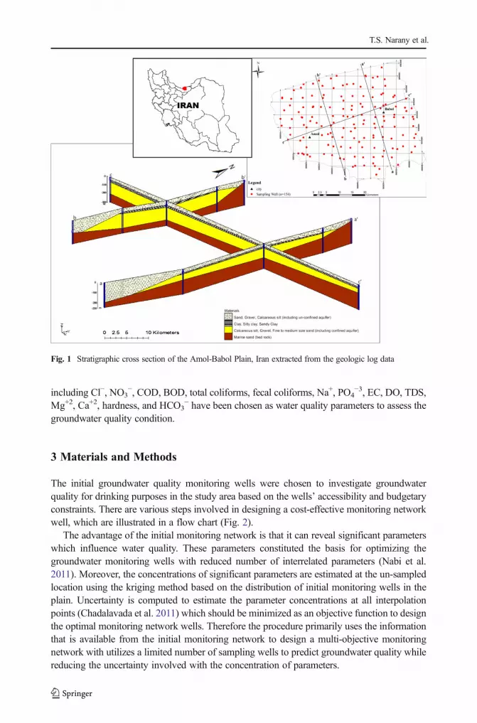
The performance of the developed optimized methodology is evaluated by using it in anexisting initial monitoring network in the Amol-Babol Plain, north Iran. The study area is oneof the fertile plain in Iran, where 67 % of land is covered by rice cultivation (Fakharian 2010).Besides agricultural activities as a main activity in the study area, the area is one of the famouseco-tourism attractions in the region. Groundwater is the main water supply due to semi-aridweather condition and overpopulation and urbanization issue in the study area, which posesintensive pressure on groundwater by over abstraction and utilization. The area of Amol-BabolPlain is about 1830 km2, approximately 45 km from north to south and 50 km from west toeast (Fig. 1). Hydrogeological investigation revealed that quaternary alluvial sediments,including deltaic and marine sediments of Haraz, Babolrud and Talar rivers covered theAmol-Babol Plain. From the western-eastern cross section (Fig. 1), the thick homogenousHaraz sediment layer gradually changes to a heterogeneous sediment layer of the Talar riverwhich consist of clay and sandy layers (Fakharian 2010). The thickness of alluvial depositsvaries from approximately 10 m near the coastal area in north to nearly 200 m in the Harazalluvial fan in the west. There are 61,498 shallow and 6,634 deep wells with various depthsfrom 3 to 198 m in the study area. The main direction of the groundwater flow is from therecharge zone in the south to the Caspian Sea in the north part of the plain. The totalabstraction of groundwater was 507 million m3 through wells, quants, and springs, of which94 % (around 342 million m3) was discharged from the wells (Jamab, 1995).
There are two major components of aquifer systems, including an unconfined aquifer whichis composed with sand, gravel and calcareous silt and covered 90% of the plain, and a confinedaquifer in calcareous silt, gravel and medium size sand, which covered 50 % of the study area.
The 154 existing monitoring wells were selected from the unconfined aquifer, which weremostly constructed by farmers for agricultural and domestic usages. 15 water quality variables,
Multi-Objective Based Approach for Groundwater Quality
including Cl−, NO3−, COD, BOD, total coliforms, fecal coliforms, Na+, PO4
−3, EC, DO, TDS,Mg+2, Ca+2, hardness, and HCO3
− have been chosen as water quality parameters to assess thegroundwater quality condition.
3 Materials and Methods
The initial groundwater quality monitoring wells were chosen to investigate groundwaterquality for drinking purposes in the study area based on the wells’ accessibility and budgetaryconstraints. There are various steps involved in designing a cost-effective monitoring networkwell, which are illustrated in a flow chart (Fig. 2).
The advantage of the initial monitoring network is that it can reveal significant parameterswhich influence water quality. These parameters constituted the basis for optimizing thegroundwater monitoring wells with reduced number of interrelated parameters (Nabi et al.2011). Moreover, the concentrations of significant parameters are estimated at the un-sampledlocation using the kriging method based on the distribution of initial monitoring wells in theplain. Uncertainty is computed to estimate the parameter concentrations at all interpolationpoints (Chadalavada et al. 2011) which should be minimized as an objective function to designthe optimal monitoring network wells. Therefore the procedure primarily uses the informationthat is available from the initial monitoring network to design a multi-objective monitoringnetwork with utilizes a limited number of sampling wells to predict groundwater quality whilereducing the uncertainty involved with the concentration of parameters.
Fig. 1 Stratigraphic cross section of the Amol-Babol Plain, Iran extracted from the geologic log data
T.S. Narany et al.

3.1 Principal Component Analysis
The principal component analysis (PCA) is a procedure for recognizing significant variablesbased on the majority of variance in a multi-dimensional dataset. This can be achieved byreducing the statistical noise in the data, exposing the outlier, and then arranging the compo-nents from the largest contribution to the least as accurately as possible with as few principalcomponents as possible. The distribution of the data is described by the linear combination ofthe components which are derived from some measure of relations such as covariance matrixor correlation (Mustapha et al. 2013). A simpler factor structure is provided using factorrotation to maximize the relationship between the variables. Therefore, varimax rotation isused to explain data easily by extracting the only components with eigenvalues higher thanone. The factor score is a measure of the statistical weight of each case on the extracted factorsand it is useful to create distribution maps based on the factor scores (Belkhiri and Narany2015). PCA can be calculated using the following equation:
γ ji ¼ fj1zi1þ fj2zi2þ⋯þ fjmþ zimþ ei j ð1ÞWhere, γ is the measured variable, fj is the factor loading, z is the factor score, e is the
residual term accounting errors, I and j is the sample number and m is the total number offactors.
3.2 Estimation Error
In geostatistical techniques the observation data are investigated to be the result of the randomfunction of regionalized variables with space coordinates, with some spatial covariance(Matheron 1963). Regionalized variables have spatial variability, and therefore the variable
Choose initial groundwater monitoring network wells
Obtain the groundwater quality parameter concentrations from observed wells
Identify significant parameters influencing groundwater quality and possible pollution
sources using principal component analysis (PCA)
Compute initial estimation error of monitoring wells using kriging method
Remove redundant wells based on the optimization assumptions in GIS environment:
- Remove wells with minimum estimation error
- Remove wells located in low and very low risk areas
- At least one well should be located in each 5*5 km
Choose the cost-effective monitoring network wells
Define three scenarios for density of monitoring wells based on EU (2001) and budgetary constraints.
Compute and compare estimation errors, standard deviation, and mass estimation
errors for each scenario
Fig. 2 Schematic diagram of the optimization of groundwater monitoring network well’s steps
Multi-Objective Based Approach for Groundwater Quality

fall between random variables and completely deterministic variables (Nunes et al. 2004).Since the regionalized variables show spatial continuity, the variation of variables is compli-cated and could not be describe by any deterministic function (Webster and Oliver 2007).Furthermore, although regionalized variables are spatially continuous, intensive sampling isexpensive and not possible. Therefore, unknown values should be estimated from data taken atspecific locations. Geostatistics use the stationary hypothesis on these procedures to estimateand simulate values for regionalized variables (Webster and Oliver 2007).
The spatial variability of regionalized variables is described by a semi-variogram, whichpractically calculates the mean square variability between two neighboring points of distance h:
γ hð Þ ¼ 1
2n hð ÞXn hð Þ
i¼1
z xþ hð Þ−z xð Þð Þ2h i
ð2Þ
Where, γ(h) is experimental variogram, z(x) and z(x+h) are the values of the variable atpoint x and at a point of distance h from point x.
Variogram modeling and estimation is extremely important for structural analysis andspatial interpolation (Li and Australia 2008). The best semivariogram model is fitted with atheoretical model, which could be chosen by using the ratio of nugget to sill. The ratio ofnugget to sill reflects the spatial heterogeneity of the data. If the ratio is close to one, then mostof the variability is results from random processes and then measurement error is high (Li andAustralia 2008).
Kriging is the best linear unbiased estimators of the surface at the specified locations topresent the possibility of estimation of the interpolation error of the regionalized variable,where there are no initial values (Jang and Liu 2004). Kriging shows some advantage comparewith other interpolation methods, since it consider: І) the number and configuration ofobservation points, ІІ) the position of observation point, ІІІ) the distance between observationpoints, and І ) the spatial continuity of the interpolated variable (Nabi et al. 2011).
The regionalized variable is assumed to be stationary without any drift, which allowsestimation of the unknown value at point xi, Z(x0) using a weighted average of the knownvalue, and it is unbiased if the sum of weights is one. Journal and Huijbregts (1978) defined thekriging system as equation 3 and 4:
Z x0ð Þ ¼Xn
i¼1
WiZ xið Þ ð3Þ
γ htAð Þ ¼X n
i¼1Wiγ hð Þ þ μ ð4Þ
Xn
i¼1
Wi ¼ 1 ð5Þ
Where n represents the number of sampled points used for the estimation, Wi is the weightassigned to the sampled point and Za is the actual value at the sampled point p, μ is theLagrange multiplier, and γ (hiA) is the average variogram between the point I and the area Awhere one extreme of the vector h is fixed in pi and the other extreme describes the area A
T.S. Narany et al.

independently. Since Wi correspond to the weights associated with the sampling points. Toensure that the estimates are unbiased the sum of the weight must be 1.
The estimation variance for Z(x0) is given by:
2Xn
i¼1
Wi γ xi;Að Þ−Xn
i¼1
Xn
i¼1
WiWJγ xi; x j� �
− γ A;Að Þ ð6Þ
Where, γ(xi,xj) is the semi-variance between the ith and jth sampling points, γ xi;Að Þ is theaverage semi-variance between the ith sampling point and area A, and γ A;Að Þ is the averagesemi-variance within the area A. The estimation variance is minimized consistent withequation (5), when:
Xn
i¼1
Wiγ xi; x j� �þ μ ¼ γ xi;Að Þ ð7Þ
This estimated value will most likely differ from the actual value at point xi, Zx0, and thisdifference is called the estimation error. Furthermore, a kriging estimator determines a varianceof estimation error (Eq 4), which quantifies the uncertainty in an estimate at each location(Jang and Liu 2004). Since the variance of the estimation error does not depend on the actualvalue of the measured variables, it is on the relative spatial distribution of the measuringlocations (Nunes et al. 2004). Therefore, the estimation variance depends on the configurationof the observation of the data points; it is possible to change by defining a different variogram.
σ2E ¼
Xn
i¼1
Wiγ hiAð Þ þ μ − γ hAAð Þ ð8Þ
Where γ (hiA) is the average variogram inside A.One of the important condition in optimality is that the variance of the estimation error
should be minimum (Ahmed et al. 2008). Although, the variance of estimation error decreaseas the number of points in the neighborhood is increased. The spatial distribution of themeasuring points also plays a significant role in the variance of the kriging estimation error(Ahmed 2004). Therefore, the variance of estimation error should be calculated prior todeciding to add a new sampling well or removing an existing well.
4 Results and Discussion
4.1 The Proposed Procedure for Designing Optimal Monitoring Network
Based on the literature, designing a monitoring network in an optimal manner is a controver-sial issue due to difficulties in the selection of spatial and temporal variations, variables to bemonitored, and the objectives of sampling (Mogheir et al. 2005; Masoumi and Kerachian2010). Despite several techniques being developed such as geostatistical technique, entropytheory, genetic algorithm, and hydrogeological evaluation, but no particular method is appli-cable to all situations. Therefore, the process of monitoring well selection should be both,representative of the entire groundwater system and also cost effective (Chadalavada et al.2011) with a minimum number of sampling wells. In this study, the new procedure has beensuggested based on the data from an existing monitoring network, where statistical analysis,
Multi-Objective Based Approach for Groundwater Quality

geostatistical techniques, hydrogeological and hydrochemical factors was integrated in a GISenvironment, as described in following optimization procedures:
4.1.1 Step One: Detection of Groundwater Contamination Source
Since the groundwater quality is influenced by different factors; detection of groundwatercontamination sources plays an important role in selecting appropriate factors for optimizinggroundwater monitoring networks. In most research, limited parameters have been applied askey factors for designing monitoring wells. For example Mogheir et al. (2006) applied salinity(Cl−), and Nitrate (NO3
−) as a major quality problem in the aquifer and Júnez-Ferreira andHerrera (2013) used hydraulic head. Based on the study (Nabi et al. 2011), multi parameterscould be combined with geostatistical analysis to define an optimized monitoring network.They suggested applying factor analysis to evaluate the interrelationship among variable, andreduce the original dataset into significant variables, which influence groundwater quality inthe basin. Therefore, in this study, the process of selecting significant factors influencegroundwater quality was addressed by applying PCA/FA on dataset collected from existingmonitoring wells (Table 1).
Following the methodology, the first two components explained 44.8 % of the totalvariance, by very high loading of Na+, Cl−, EC, and TDS, which show groundwater salinity,and Mg2+, Ca2+, and hardness which show groundwater hardness. These results suggest thatthe quality of groundwater in Amol-Babol Plain mainly is influenced by natural
Table 1 Principal component matrix for each parameter analyzed for groundwater
Parameter Rotated Component Matrix
Component
1 2 3 4 5
Cl− .754 .070 −.049 .079 −.078NO3
− −.173 .111 .188 −.040 .788
COD .135 .104 −.123 .891 −.034BOD .095 .019 .147 .911 .068
Total coliform .075 .071 .970 .025 .063
Fecal coliform .054 .062 .968 −.001 .066
Na+ .913 −.102 .013 .035 −.188PO4
3− .090 −.560 −.020 .102 .098
EC .939 .192 .109 .114 .067
DO −.366 .014 −.252 −.056 .592
TDS .937 .153 .130 .100 .049
Mg2+ .338 .745 .014 .022 −.075Ca2+ −.028 .745 .084 .199 .292
Hardness .189 .922 .057 .144 .167
HCO3− .323 .003 .110 .136 .589
Eigenvalue 4.2 2.48 1.90 1.52 1.18
% Variance 28.26 16.57 12.70 10.15 7.85
Total Variance 28.26 44.84 57.54 67.7 75.56
T.S. Narany et al.
contamination. The second three components explained by 30.7 % of the total variance, whichindicate anthropogenic contamination by high loading of total and fecal coliforms, COD,BOD, and NO3
−. Intensive agricultural activities would dominate the input of these chemicals,and biological pollution into groundwater, especially shallow wells in the north side of studyarea. In order to develop the optimized groundwater monitoring network, two different caseswere defined based on the PCA/FA results in the study area, including natural contaminationfactors (NCF) and anthropogenic contamination factors (ACN). The spatial variability of thesecases was defined by extracting factor scores and calculating experimental and theoreticalvariograms using the kriging method. Each defined case consists of three different scenarios,which are determined based on the following criteria.
4.1.2 Step Two: Consideration of the Potential Risk to the Aquifer from Contamination
Since the natural groundwater quality is mostly influenced by the geochemical processes basedon the reaction between infiltration water with the soils and rock-forming minerals and also byhuman activities which superimpose pollution on the groundwater, it is impossible to choosegroundwater monitoring wells without considering hydrogeological conditions of the aquiferand also spatial variety of land use activities. A combination of a vulnerability map and akriging variance map in GIS environment was suggested as an approach to design the optimalnetwork by Baalousha (2010). He mentioned that the area with high vulnerability to pollutionrequires an adequate number groundwater monitoring wells. Kriging variance may indicatewhether the number of wells is adequate to cover the study area, but cannot determine zonesthat need to be monitored. Therefore, the potential risk of groundwater to pollution should beconsidered as a significant factor in the optimization of monitoring wells, besides the role ofwater quality data from monitoring wells.
Since the majority (around 80 %) of study area is agricultural lands, utilization of organicand inorganic fertilizers by farmers may threaten the groundwater quality. The adverse impactof human activities is obvious where the presence of total and fecal coliforms and nitrate haddegraded the groundwater quality, mostly in shallow agricultural wells in north and centralsides of the Amol-Babol Plain (Table 1). Sheikhy Narany et al. (2013) integrated land use mapwith vulnerability map for mapping the potential risk of aquifer contamination in Amol-BabolPlain. Based on their study, the majority (around 88 %) of the aquifer was classified in the lowand moderate low risk index areas. Only a limited area (less than 11 %) was classified asmoderate risk index area.
4.1.3 Step Three: Determination of Density of Monitoring Network Wells
The design of monitoring network wells in the absence of primary data is highly subjec-tive. Chadalavada et al. (2011), mentioned that the maximum number of wells in aparticular management period is subjected to the budgetary constraints. The existingmonitoring data in the study area consist of 154 monitoring wells. The EU working groupon the implementation of the water directive recommends a density of about 1point/25 km2, where the groundwater body is expected to be Bunder pressure^ and 1 point/100 km2 (Rentier et al. 2006). Khairy (2009) suggested that the normal distance of themonitoring well is around 5 km.
In the initial monitoring network, the mean distance between sampling wells is 2060 m,which varied from a minimum of 197 m to a maximum of 4304 m. Based on the criteria about
Multi-Objective Based Approach for Groundwater Quality

density of monitoring network, with an area of 1830 km2, the number of sampling wells wassuggested to be around 75 in Amol-Babol Plain. The maximum numbers of monitoring wellsare presented as 130, 100, and 74 sampling wells in each case.
4.1.4 Step Four: Calculation of Spatial Estimation Variance
Spatial concentration estimation of variances had also been calculated using the krigingmethod at the interpolated location. Based on the optimization assumption, the optimizedmonitoring network should minimize the spatial concentration estimation variance by addingsampling wells where the uncertainty is high (Chadalavada et al. 2011). Sampling pointswithin areas of small estimation variance could also be excluded from the monitoring network,because the smaller the difference between measured and estimated values, the lesser theimportance of the specific sampling well for the simulation of groundwater quality distribution(Theodossiou and Latinopoulos 2006). In the existing monitoring network, the estimation errorbased on the NCF and ACN varied from 0.0035 to 2.4330 and from 0.0106 to 2.3630,respectively (Table 2).
4.1.5 Step Five: Identification the Potential Monitoring Wells Locations
All the criteria mentioned previously, should be considered in identifying the potentialmonitoring well locations. Exclusion of sampling wells require very careful thought since thiscould unpredictably increase estimation error reversing the actual criteria that led to theexclusion in the first place (Theodossiou and Latinopoulos 2006).
GIS software is a reliable tool for selecting excluding sampling wells based on theestimation error, distance of sampling wells, and potential risk of aquifer to contamina-tion. The priority of the sampling wells to be excluded from monitoring network wasdetermined based on the optimization criteria within GIS environment. The optimizationcommands were defined based on the sampling wells with minimum nearest distance,lowest estimation errors, and lowest risk of pollution (Fig. 3). After running eachcommand, the new nearest distance and estimation error were computed. The minimiza-tion process continues until it reach to a maximum acceptable sampling well of eachscenario.
Table 2 Results of the optimal network design for monitoring water quality at Amol-Babol Plain
Case Scenario (well number) Kriging Estimation Error Standard Deviation Mean Of well Distance
Minimum Mean Maximum
NCF 154 0.0035 0.5777 2.4334 0.4777 2060
130 0.0047 0.6524 2.4956 0.4982 2500
100 0.0141 0.7292 2.4660 0.5370 3160
74 0.0190 0.7976 2.7529 0.6326 3700
ACF 154 0.0106 0.8416 2.3629 0.4925 2060
130 0.0111 0.9356 2.3378 0.4819 2450
100 0.0561 1.0104 2.5163 0.5102 3180
74 0.0090 1.0431 2.5390 0.5452 3680
T.S. Narany et al.

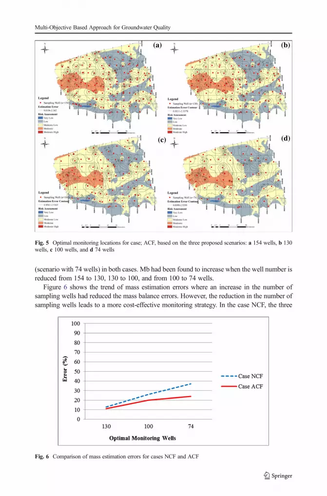
The specific optimization command was defined and performed for all scenarios in eachcase (Figs. 3). Areas of denser estimation error contours (Figs. 4 and 5) may indicate either thesampling wells with significant estimation error or the lack of measurement. Therefore, suchmonitoring wells are considered to be very important and indicate areas where there monitor-ing network needs to be denser (Theodossiou and Latinopoulos 2006). On the other hand,sampling wells in the sparse estimation error contours are the best choice to be excluded frommonitoring network. Depending on the type of contaminant sources, which may be natural oranthropogenic, the estimation error contours show different densities (Figs. 4 and 5). In theNCF case, high differences between measured and estimated natural contamination of waterwas recognized in the eastern side. On the other hand, sampling wells from the eastern sideshould be eliminated very carefully due to higher uncertainty in estimation (Fig. 4a). In theACF case, estimation error contours show high uncertainty in central and northern sides of theplain, probably due to the position of shallow wells, which are located in the northern side(Fig. 5a).
Shallow wells are usually threatened by agricultural and residential runoffs, and moresusceptible to by anthropogenic pollution compared to the deep wells. Choosing differentscenarios of monitoring wells in the network and identifying redundant monitoring wellsin the existing network, leads to examining the redundancy reduction in the monitoringnetwork. The performance of the developed network design may be evaluated by the meanof estimation error and standard deviation of each scenario is calculated in each step ofprocess (Table 2).
1, D; nearest wells distance
2, E; Estimation Error
3, R; Potential aquifer risk to pollution
Case: NCF
Scenario: 130 wells
YES
Is the well number reach to goal?
NO
Calculated new estimation errors and wells distance
Removed selected wells
Finish
First Command: "D1" <=1000 AND "E
2" <= 0.5 AND "R
3" <=Moderate
Second Command: "D" <=1500 AND "E" <= 0.5 AND "R" <=Moderate -low
Third Command: "D" <=2000 AND "E" <= 0.5 AND "R" <=low
Fourth Command: "D" <=2600 AND "E" <= 0.6 AND "R" <=low
Third repeat
Second repeat
Fourth repeat
Fig. 3 Example of minimization command for NCF case in the GIS software
Multi-Objective Based Approach for Groundwater Quality

4.2 Efficiency Evaluation of Designed Network
4.2.1 Mass Estimation Error
The efficiency of the developed designed models is evaluated in terms of the mass estimationerror for the illustrative problems (Chadalavada and Datta 2008), which is the error betweenthe contaminant mass estimated using the existing monitoring and designed monitoringnetwork (Chadalavada et al. 2011). If minimization of error is not a clear objective of theproposed optimization scenarios, the acceptability of a designed model could be established byassuming that the boundary of the study area and parameter values are deterministic in nature.Therefore, the exact mass of the contamination is assumed to be known. This mass is estimatedbased on the contamination concentration at existing monitoring wells using the kriginginterpolation method. The difference between mass estimation obtained from optimal moni-toring network (Mj) and mass estimation obtained from initial monitoring well (Mi) is the massbalance estimation error (Mb) to the designed monitoring network (Reed et al. 2000):
Mb ¼ absMi −M j
Mi
� �� �� 100 ð9Þ
The mass balance errors were calculated between the estimated M (existing monitoringwell) and M1 (scenario with 130 monitoring wells), M2 (scenario with 100 wells), and M3
(a) (b)
(c) (d)
Fig. 4 Optimal monitoring locations for case; NCF, based on the three proposed scenarios: a 154 wells, b 130wells, c 100 wells, and d 74 wells
T.S. Narany et al.
(scenario with 74 wells) in both cases. Mb had been found to increase when the well number isreduced from 154 to 130, 130 to 100, and from 100 to 74 wells.
Figure 6 shows the trend of mass estimation errors where an increase in the number ofsampling wells had reduced the mass balance errors. However, the reduction in the number ofsampling wells leads to a more cost-effective monitoring strategy. In the case NCF, the three
(a) (b)
(c) (d)
Fig. 5 Optimal monitoring locations for case; ACF, based on the three proposed scenarios: a 154 wells, b 130wells, c 100 wells, and d 74 wells
Fig. 6 Comparison of mass estimation errors for cases NCF and ACF
Multi-Objective Based Approach for Groundwater Quality

different scenarios including 130, 100, and 74 wells resulted in 12.9, 26.9, and 37 % massbalance error, respectively. These show that around 88, 74, and 63 % capacity to naturalcontaminant mass detection can be achieved for each scenario. In the case of ACF, threescenarios of 130, 100 and 74 wells, show 11.1, 20, and 23.9 % mass balance error, this showsaround 89, 80, and 77 % of capacity to anthropogenic contaminant mass detection at eachoptimal location, respectively. The mass estimation error in the NCF case is higher than in theACF case. This is due to natural contaminants being widely spread in the study area comparedto anthropogenic contaminant, which mostly accumulates in residential areas and agriculturallands, due to intensive human activities. Therefore, denser monitoring wells (scenario with 100monitoring well) can be used in the case NCF case and a scenario with 74 monitoring wellscan be used for the ACF case to detect the mass present in the system with around 23–26 %errors.
Intersection of selected scenarios including 100 wells for the NCF case and 74 wells for theACF case in the GIS environment represents 60 common sampling wells with the samecoordinate systems in both cases (Fig. 7). Therefore, in the case of groundwater qualitymonitoring strategy for both natural and anthropogenic contaminant sources, the total numberof 114 sampling wells, could be proposed, which shows 14.8 % mass balance error. Thisshows the natural and anthropogenic contaminant mass detection capacity of around 85 % canbe obtained from only 114 sampling wells (Fig. 7). The mean distance is 2760 m for 114sampling wells in the study area. These results indicate the significant role of redundancy anduncertainty in the monitoring network design.
Fig. 7 Optimal monitoring locations based on 114 sampling wells
T.S. Narany et al.

5 Conclusion
In the absence of primary data, groundwater monitoring network wells show significantredundancy or uncertainty of information. Therefore, the number and distribution of samplingwells should be selected in the optimal conditions to provide maximum information withminimum monitoring location. In this study, the proposed information-cost-effective monitor-ing network wells used preliminary data from initial existing monitoring wells to obtain, І)significant contaminant factors that influence groundwater quality using principal componentanalysis (PCA), and ІІ) uncertainty associated with the monitoring network using estimationerror in the kriging interpolation method. Moreover, the methodology suggested identifyingareas with high pollution potential as an important factor in monitoring network optimization.Three optimal number of sampling wells scenarios of 130, 100, and 74 wells were definedbased on the monitoring wells density criteria and contaminant sources in the study areaincluding, natural and anthropogenic contaminant factors. The performance of the proposedscenarios was evaluated by comparing the mass estimation error for each case. Although thescenarios with 100 and 74 sampling well for natural and anthropogenic contaminant factorsshow acceptable mass estimation error, respectively. The total number of 114 sampling wellswas chosen as optimal monitoring network wells by combining the best scenarios of each casein GIS environment. The reduction in the number of monitoring well shows that the contam-inant mass detection capacity of around 86 % can be obtained from only 114 wells instead of154 initial sampling wells. The redesigned network considers the budgetary constraint byimposing a limit on the maximum number of sampling wells.
Acknowledgments The authors acknowledge the Soil and Water Pollution Bureau of the Department ofEnvironment (DOE) in Iran for their financial support through a contract with Amirkabir University ofTechnology (AUT), Tehran, Iran. The financial support by DOE and the laboratory data and analyses providedby AUT are gratefully acknowledged. Special thanks are due to Mr. A. S. Mohammadlou for his sincerecooperation in providing the data.
References
Ahmed S (2004) Geostatistical estimation variance approach to optimizing an air temperature monitoringnetwork. Water Air Soil Pollut 158(1):387–399
Ahmed S, Jayakumar R, Salih A (2008) Groundwater dynamics in hard rock aquifers: sustainable managementand optimal monitoring network design. Springer
Baalousha H (2010) Assessment of a groundwater quality monitoring network using vulnerability mapping andgeostatistics: a case study from heretaunga plains, New Zealand. Agric Water Manag 97(2):240–246
Belkhiri L, Narany TS (2015) Using multivariate statistical analysis, geostatistical techniques and structuralequation modeling to identify spatial variability of groundwater quality. Water Resour Manag 1–17
Chadalavada S, Datta B (2008) Dynamic optimal monitoring network design for transient transport of pollutantsin groundwater aquifers. Water Resour Manag 22(6):651–670
Chadalavada S, Datta B, Naidu R (2011) Uncertainty based optimal monitoring network design for a chlorinatedhydrocarbon contaminated site. Environ Monit Assess 173(1–4):929–940
Datta B, Chakrabarty D, Dhar A (2009) Optimal dynamic monitoring network design and identification ofunknown groundwater pollution sources. Water Resour Manag 23(10):2031–2049
Dhar A, Patil RS (2012) Multiobjective design of groundwater monitoring network under epistemic uncertainty.Water Resour Manag 26(7):1809–1825
Fakharian K (2010) Hydrogeology report of Amol-Babol plain, study of prevention, control and reduce pollutionof Amol-Babol aquifer. Department of environment of Iran, through a contract with Amirkabir University ofTechnology
Multi-Objective Based Approach for Groundwater Quality

Jamab (1995) Soil and land classification and land resource evaluation (Persian version). Jamab Consluting Co.Ministry of Energy, Iran
Jang CS, Liu CW (2004) Geostatistical analysis and conditional simulation for estimating the spatial variabilityof hydraulic conductivity in the choushui river alluvial fan, Taiwan. Hydrol Process 18(7):1333–1350
Journel AG, Huijbregts CJ (1978) Mining Geostatistics. Academic Press, London, pp. 600Júnez-Ferreira H, Herrera G (2013) A geostatistical methodology for the optimal design of space–time hydraulic
head monitoring networks and its application to the Valle de Querétaro aquifer. Environ Monit Assess185(4):3527–3549
Khairy H (2009) Groundwater monitoring network optimization using geostatistical methods (case studyqaemshahr-joybar plain) (Persian ed.). Mazandaran Regional Water Company, Mazandaran, Iran
Li J, Australia G (2008) A review of spatial interpolation methods for environmental scientists, vol 137. GeosciAust Canberra
Masoumi F, Kerachian R (2010) Optimal redesign of groundwater quality monitoring networks: a case study.Environ Monit Assess 161(1–4):247–257
Matheron G (1963) Principles of geostatistics. Econ Geol 58(8):1246–1266Mogheir Y, De Lima JLMP, Singh VP (2005) Assessment of informativeness of groundwater monitoring in
developing regions (Gaza strip case study). Water Resour Manag 19(6):737–757Mogheir Y, Singh V, de Lima J (2006) Spatial assessment and redesign of a groundwater quality monitoring
network using entropy theory, Gaza strip, Palestine. Hydrogeol J 14(5):700–712Mogheir Y, De Lima JLMP, Singh VP (2009) Entropy and multi-objective based approach for groundwater
quality monitoring network assessment and redesign. Water Resour Manag 23(8):1603–1620Mustapha A, Aris A, Juahir H, Ramli M (2013) Surface water quality contamination source apportionment and
physicochemical characterization at the upper section of the jakara basin, Nigeria. Arab J Geosci 6(12):4903–4915. doi:10.1007/s12517-012-0731-2
Nabi A, Gallardo AH, Ahmed S (2011) Optimization of a groundwater monitoring network for a sustainabledevelopment of the maheshwaram catchment, India. Sustainability 3(2):396–409
Nunes L, Cunha M, Ribeiro L (2004) Groundwater monitoring network optimization with redundancy reduction.J Water Resour Plan Manag 130(1):33–43
Odom KR (2003) Assessment and redesign of the synoptic water quality monitoring network in the great smokymountains national park
Reed P, Minsker B, Valocchi AJ (2000) Cost‐effective long‐term groundwater monitoring design using a geneticalgorithm and global mass interpolation. Water Resour Res 36(12):3731–3741
Rentier C, Delloye F, Brouyère S, Dassargues A (2006) A framework for an optimised groundwater monitoringnetwork and aggregated indicators. Environ Geol 50(2):194–201
Rouhani S, Hall TJ (1988) Geostatistical schemes for groundwater sampling. J Hydrol 103(1):85–102Sheikhy Narany T, Ramli MF, Aris AZ, Sulaiman WNA, Fakharian K (2013) Spatial assessment of groundwater
quality monitoring wells using indicator kriging and risk mapping, amol-babol plain, Iran. Water 6(1):68–85Theodossiou N, Latinopoulos P (2006) Evaluation and optimisation of groundwater observation networks using
the Kriging methodology. Environ Model Softw 21(7):991–1000Webster R, Oliver MA (2007) Geostatistics for environmental scientists. John Wiley & SonsZaidi FK, Ahmed S, Dewandel B, Maréchal J-C (2007) Optimizing a piezometric network in the estimation of
the groundwater budget: a case study from a crystalline-rock watershed in southern India. Hydrogeol J 15(6):1131–1145
T.S. Narany et al.


