Embed Size (px)
Citation preview

Assessment of the Potential Impacts of Climate Variability and Shocks on Zimbabwe’s
Agricultural Sector: A Computable General Equilibrium (CGE) Analysis
15 December 2018
By: Pablo Benitez Brent Boehlert
Rob Davies Dirk van Seventer
Melissa Brown
Pub
lic D
iscl
osur
e A
utho
rized
Pub
lic D
iscl
osur
e A
utho
rized
Pub
lic D
iscl
osur
e A
utho
rized
Pub
lic D
iscl
osur
e A
utho
rized

i
Acknowledgements
The report was prepared by a World Bank team led by Pablo Benitez and Melissa Brown in collaboration
with Industrial Economics, incorporated as part of Zimbabwe’s Climate Change Technical Assistance (TA)
Program. The main contributors to the report are Pablo Benitez, Brent Boehlert, Rob Davies, Dirk van
Seventer, and Melissa Brown. The Climate Change TA received strategic guidance from Washington
Zhakata (Director of the Climate Change Management Department), Kudzai Ndidzano (Acting Deputy
Director) and Lawrence Mashungu (NDC focal point) at the Ministry of Lands, Agriculture, Water,
Climate and Rural Resettlement and Veronica Jakarasi (Manager, Climate Finance, IDBZ). Key guidance
for the analysis was also provided by staff from the Ministry of Lands, Agriculture, Water, Climate and
Rural Resettlement during a consultation workshop held on April 6, 2018. The team is also grateful to
Johannes Herderschee, Sebastien Dessus, Willem G. Janssen, Marko Kwaramba, Azeb Fissha, Holger A.
Kray, Rob Swinkels, Fadzai Naome Mukonoweshuro, Mandi Rukuni, and Gibson Guvheya for their
guidance and contributions. Special mention to World Bank’s Management including Paul Noumba Um,
Mukami Kariuki, Magda Lovei, Iain Shuker, Mark Cackler and peer-reviewers: James Thurlow and Will
Martin (International Food Policy Research Institute), and Govinda Timilsina, Ioannis Vasileiou and
Tobias Baedeker (World Bank). The financial support of the Climate Investment Readiness Program for
Africa (CIRPA) of GIZ, Zimbabwe’s Reconstruction Fund (ZIMREF), and the Global Food Crisis Fund is
gratefully acknowledged.
This work is a product of the staff of the World Bank with external contributions. The findings, interpretations, and conclusions
expressed do not necessarily reflect the views of the Bank, its Board of Executive Directors, or the governments they represent.

ii
Table Of Contents
Acronyms ..................................................................................................................................................... iv
Executive Summary .................................................................................................................................. ES-1
1. Introduction ..................................................................................................................................... 1
1.1 Objectives of this Analysis .................................................................................................. 2
1.2 Approach taken in this Report ............................................................................................ 3
1.3 Organization of this Report ................................................................................................. 4
2. Background: Climate Change and Zimbabwe’s Agricultural Sector................................................. 5
2.1 Agriculture in Zimbabwe ..................................................................................................... 5
2.2 Climate Change in Zimbabwe and Impacts on the Agricultural Sector .............................. 6
2.3 The Tension Between Investments for Economic Recovery and Climate Resilience ......... 8
3. Scenarios and Adaptation Options .................................................................................................. 9
3.1 Climate Scenarios ................................................................................................................ 9
3.2 Macroeconomic Scenario ................................................................................................. 11
3.3 Adaptation Options and Investment Packages ................................................................. 12
4. Findings .......................................................................................................................................... 14
4.1 Climate Change Impacts on Crop Yields ........................................................................... 14
4.2 Economy-wide Impacts of Climate Change and Benefits of Adaptation .......................... 16
4.2.1 Impacts under Weather and Climate Shocks ....................................................... 16
4.2.2 Benefits of Adaptation ......................................................................................... 17
4.2.3 Nature-Based Solutions for Increased Resilience ................................................ 19
5. Summary and Recommendations .................................................................................................. 20
5.1 Summary of Findings ........................................................................................................ 20
5.2 Policy Recommendations .................................................................................................. 21
References .................................................................................................................................................. 24
Appendix A. Modeling Framework ............................................................................................................. 26
A.1 Overview ........................................................................................................................... 26
A.2 Spatial Scale ...................................................................................................................... 26
A.3 Crop Model ....................................................................................................................... 28

iii
A.4 Economy-wide Model ....................................................................................................... 30
Appendix B. Description of Crop Modeling Approach .......................................................................... 33
B.1 Model Structure ................................................................................................................ 33
B.2 Inputs and Model Calibration ........................................................................................... 34
B.3 Model Outputs .................................................................................................................. 34
Appendix C. Economy-wide Modeling and the Underlying Social Accounting Matrix ......................... 35
Appendix D. Macroeconomic Balances and Domestic Linkages ........................................................... 39
D.1 Current Macroeconomic Balances .................................................................................... 39
D.2 Land Issues ........................................................................................................................ 41
D.3 Some Accounting .............................................................................................................. 42
D.4 Strengthening Domestic Linkages ..................................................................................... 42
D.5 Treatment of Investment Scenario Costs in the CGE ........................................................ 46
Appendix E. Effects of the Structure of the Economy................................................................................. 50
E.1 Effects of a More Integrated Economy ............................................................................. 50
E.2 Fixed versus Floating Exchange Rates ............................................................................... 52
Appendix F. Development of Investment Packages and Integration into CGE ........................................... 54
F.1 Development of Packages................................................................................................. 54
F.2 Treatment of Investment Scenario Costs in the CGE ........................................................ 55
Appendix G. Implementation of Adaptation Investments in the CGE Model ............................................ 58
Appendix H. Results of Engineering Cost Analysis ..................................................................................... 62
H.1 Impacts on Farm Revenues ............................................................................................... 62
H.2 Benefits from Adaptation ................................................................................................. 63
H.2.1 Adaptation Option 1: Irrigation ........................................................................... 63
H.2.2 Adaptation Option 2: Improved Crop Variety and Increased Inputs ................... 65
Appendix I. Study Caveats and Recommended Further Analysis .............................................................. 66
I.1 Study Caveats .................................................................................................................... 66
I.2 Recommended Further Analysis ....................................................................................... 68
Appendix J. Macroeconomic Effects .......................................................................................................... 70

iv
Acronyms
AER Agro-Ecological Region
B-C Benefit-Cost
BAU Business as Usual macroeconomic scenario
CGE Computable General Equilibrium
CMI Climate Moisture Index
CMIP3 Coupled Model Intercomparison Project phase 3
CMIP5 Coupled Model Intercomparison Project phase 5
GCM General Circulation Model
GDP Gross Domestic Product
ECRAI Enhancing the Climate Resilience of Africa’s Infrastructure
FAO U.N. Food and Agriculture Organization
FTLRP Fast Track Land Reform Programme
ha Hectares
HI Harvest Index
IFPRI International Food Policy Research Institute
INT Integrated Economy macroeconomic scenario
IPCC Intergovernmental Panel on Climate Change
IWR Irrigation water requirement
LS Large Scale Farms
LSCF Large Scale Commercial Farming
O&M Operations and Maintenance
R&D Research and development
SAM Social Accounting Matrix
SH Small Holder Farms
SSC Small Scale Commercial
USDA U.S. Department of Agriculture

ES-1
Executive Summary
Zimbabwe has a highly variable climate and is very vulnerable to the anticipated impacts of climate
change in southern Africa. Climate change is projected to not just change the long-term average
temperature and precipitation in the region, but also change their variability, particularly when it comes
to precipitation. These projected rising temperatures and more variable rainfall will have a major
impact on agricultural production in Zimbabwe during the period 2017-2030 and beyond.
This study aims to increase our understanding of the economic effects of climate change impacts on the
agricultural sector in Zimbabwe. The study assesses both the effects of changes in average temperature
and precipitation, as well as the effects of increases in variability. The latter is important because it links
to climate shocks (i.e., extreme weather events) in Zimbabwe. The study also explores the economy-
wide benefits of a set of priority climate change adaptation investments in the agricultural sector.
In order to quantitatively evaluate the impacts of climate change on Zimbabwe’s agricultural sector and
economy, this study combines climate change models with biophysical and economy-wide modeling.
Acknowledging the uncertainty of climate change, we consider impacts and benefits under three
different climate scenarios through 2030 (dry/hot, medium, and wettest). Out of many possible
adaptation options, two are examined in detail: the first scales up investments in irrigation while the
second invests in research and development (R&D) of new, more climate resilient crop varieties as well
as increased input (e.g. fertilizer) application. These two adaptation options are translated into
investment packages. Their impacts are evaluated using a Computable General Equilibrium Model (CGE)
representing Zimbabwe’s economy. The benefits of the different adaptation options are evaluated
relative to a “no adaptation” base option.
We find that regardless of climatic scenario, the effects of climate change on Gross Domestic Product
(GDP) are significant (Table ES-1).
Tab le ES -1 : Perce ntage ch ange in Z i mbabwe ’s 2 030 GDP under a n o -adaptat ion case , and under tw o
d i f ferent adaptat i on opt i on s , for three c l i mate scena r ios and one contr ol scena r io
Adaptation Option
Climate Scenario
Control Dry/Hot Medium Wet No Adaptation NA -2.3% -1.5% 1.4%
Irrigation 0.8% -1.1% -0.4% 2.0%
R&D and Inputs 1.6% -0.5% 0.4% 2.9%
Under the “no adaptation” base case, impacts under a dry/hot climate future can be up to 2.3% of
Zimbabwe’s 2030 GDP, or approximately $370 million annually based on 2016 GDP levels. On the other
hand, climate change may bring opportunities – under a wet scenario, GDP may rise by up to 1.4%.

ES-2
Adapting to climate change is a “win-win” situation for Zimbabwe, whether it means avoiding damages
under a dry scenario or enhancing GDP gains under a wetter future. Of the two adaptation options
considered, enhancing R&D and input application has a significantly larger effect on GDP than
investment in irrigation: under the wet scenario, the gains are higher for this option and under the dry
scenario, the losses are smaller. This R&D adaptation option also has a lower investment cost, making
the return on investment much higher than for the irrigation option.
Table ES-1 also shows that these two adaptation options are sensible regardless of whether climate
change occurs or not. The R&D and irrigation investments increase GDP by 1.6% and 0.8% under the “no
climate change” control scenario, which translates to approximately $260 and $130 million annually
based on 2016 GDP.
Several policy considerations and interventions are suggested by this study. We list some of them below.
It is important to emphasize that the study was limited in scope and the suggestions emanating from it
are broad. Clearly, implementing any specific policies would require further detailed analysis. For
example, we have shown that irrigation is a beneficial in in addressing climate change impacts. However,
implementing an irrigation strategy would require all the detailed studies of hydrology, terrain,
engineering, finance and other aspects that precede any irrigation project.
The suggested interventions all stem from the observation that climate change will significantly
impact Zimbabwe’s GDP. Climate change adaptation is ‘win-win’, and thus essential regardless of
climate futures; even in the wettest scenario, these investments make economic sense. Although the
direct impacts are on agriculture, they are multiplied up through its forward and backward linkages to
the rest of the economy. These indirect effects in turn feed back to the agricultural sector. The overall
impact on GDP is thus greater than the direct impact.
Both macroeconomic and sector specific policies are required. The foregoing observation highlights
that the scope for climate change adaptation interventions is the whole economy, not simply those
parts that are directly vulnerable to climate change. While some will target sectors, others are
macroeconomic in nature, related to the management of the overall economy.
Macroeconomic Policy Recommendations
• Climate adaptation policies and growth policies go hand in hand. While Zimbabwe’s most
pressing current economic concern is how to grow the economy, it is sensible to consider
climate change when designing growth policies.
• An integrated and more diversified economy is more resilient to climate change. Our
investigations suggest that the economy is more resilient to climate change the more integrated
and diversified it is.
• Attention should also be paid to sectors less vulnerable to climate change. Many adaptation
interventions will rightly focus on shock-proofing agriculture; however, attention should be paid
to less vulnerable sectors, such as mining, services, and tourism. The stronger these sectors are,
the more they can cushion the impact of climate shocks on agriculture and agricultural exports.

ES-3
• Open trade is necessary to reduce negative climate impacts. The study suggests that trade
policies are important for determining the impact of climate shocks. Climate shocks reduce
agricultural supplies. In the absence of other sources of supply, the prices of agricultural
products will rise, causing the sector to draw in more of Zimbabwe’s resources, even though its
productivity and thus food security are declining. This perverse effect can be avoided if imports
can fill the gap.
Sector-Specific Recommendations
• Non-structural interventions provide higher returns than infrastructure investments.
Interventions that require large scale investment can take time to roll out and are associated
with high direct and opportunity costs. Soft-interventions, such as better agricultural extension
or adoption of new varieties and farming practices can be cheaper, more flexible and quicker,
and therefore provide higher returns.
• Integrated management of natural resources (land and water) helps to build resilience while
managing other environmental challenges. Investments in integrated landscape management,
focusing on improved and diversified livelihoods, soil and land protection, and forestry and
watershed management would enable an improved and efficient response to climate risks.
• Improved water and crop management will be needed to compensate for possible
abandonment of rainfed crop and livestock production in certain regions. Under climate
change, reduced and more variable precipitation will threaten the viability of rainfed agriculture
and livestock production in some regions of Zimbabwe. Compensating for this loss will require
increasing the supply of agricultural products through various adaptation measures.

1
1. Introduction
Zimbabwe has a highly variable climate and is very vulnerable to the anticipated impacts of climate
change in southern Africa. Agricultural production in the country is prone to extreme weather events
(i.e., droughts and floods), which have major negative impacts on food security as well as on other areas
such as hydro-power generation, the agroprocessing industry and urban and rural water supply.
Climate change is projected to have a major impact on agricultural production in Zimbabwe between
2017-2030 and beyond. Climate change will manifest itself in changes to average weather conditions
over time, as well as increased variability of these same conditions. These manifestations of climate
change are set to affect agriculture dramatically. Crop yields will change and major droughts could
become twice as frequent, with adverse impacts on inclusive growth and poverty alleviation in rural
areas.
Most recently, the El Niño experienced during the 2015/16 season produced low rainfall and drought
conditions in the country, which led to a large drop in agricultural production and left a number of
districts with a food deficit and receiving food aid. At the peak of the lean season following this
2015/2016 El Niño event, and prior to the harvest of the 2016/17 season, an estimated 4 million people
suffered income deficits at the household level and were in need of temporary food aid.1
The direct impact of climate change on crop yields and water management is well documented, but
there are no estimates of the indirect effects at the aggregate sectoral and economy levels in
Zimbabwe.2 A deeper understanding of these indirect effects is important for a richer policy formulation
to combat climate change in Zimbabwe. For example, estimates of indirect effects are required if the
public sector in Zimbabwe has to decide whether to invest in a particular measure to mitigate the
impact of climate change on agricultural production – let’s say irrigation – or to invest in economic
activities that may offer employment after downturns in the agricultural sector. Accordingly, there has
been increased attention in development thinking that includes the importance of the rural nonfarm
economy as an integral component of rural development, rather than focusing solely on agricultural
production activities.
1 Note that it is important to distinguish El Niño events from long-term climate change. While the manifestations
of an El Nino event and future climate change could be similar (which is why we present an El Nino event here by way of an example) they are two distinct meteorological phenomena and should be treated as such.
2 Direct effects of climate change such as reduced crop yields can have indirect effects on other sectors through
linkages within the economy. For instance, food processing within the manufacturing sector may be dependent on agricultural output, and reduced incomes for farmers will affect consumer spending within Zimbabwe. Indirect effects capture these other impacts.

2
Additionally, Zimbabwe is affected by a variety of economic and climatic shocks, including changes in
commodity prices, exchange rates and changes in weather patterns. Weather-related shocks – floods
and droughts – affect the poor much more than other income groups, and it has been well-established
that the impacts of climate change will affect the poor disproportionately. The poor are predominantly
located in rural areas and depend directly or indirectly on agricultural production.
The impact of weather-related shocks on the poor appears to have changed over time. A comparison of
the impact of the drought in 1992 to the impact of the El Niño weather pattern in 2016 is illustrative.
The drought of 1992 was less severe than that of 2016, but the 1992 event had a larger impact on the
economy because the agricultural sector was more integrated with the manufacturing and services
sectors. At that time, backward and forward linkages to the agricultural sector were denser and hence
the crisis in the agricultural sector had a deeper impact on the manufacturing and services sectors, and
the economy as a whole. The El Niño-induced drought in 2016 may have been more severe than in 1992,
but the impacts were also more isolated given the long term decline in agricultural output since the
1990s. Nonetheless, this more recent event may also have a more lasting impact on poverty. Compared
to 1992 when the economy was more vibrant, the more constrained economic climate of 2016 was
marked by a restricted portfolio of off-farm livelihoods options for rural people. For example wage labor
or income generating opportunities in rural areas and small towns had decreased dramatically
compared to 1992 and did not offer income opportunities to those who suffered from a loss of
agricultural income. Hence to maintain the minimum consumption pattern – food principally – the poor
reduced their capital stock, often at fire-sale prices. So while the 1992 event may have had greater
impacts on the economy as a whole, the 2016 event may be associated with longer lasting impacts on
poverty.
As Zimbabwe continues to shape its future policy and investment framework – which would be expected
to deepen linkages between agriculture, manufacturing and service sectors – there will be a need to
ensure the impacts of climate change and variability are well understood. Implementation of policy
recommendations to deepen linkages between the agricultural and the manufacturing and services
sectors could boost employment and poverty alleviation, but may not immediately reduce the
vulnerability of the poor to weather-related shocks as immediate income-earning opportunities for the
poor who lose their income during an agricultural down turn may still be limited. Furthermore weather
related shocks in a larger agro-based manufacturing sector could deepen the economy-wide impact of a
contraction in the agricultural sector in line with the experience of the 1990’s. In this context it is
important to quantify both effects to inform the policy debate on measures to mitigate and/or adapt to
weather related shocks affecting the agricultural sector.
1.1 Objectives of this Analysis
This study aims to increase the understanding of the economic effects of climate change in Zimbabwe,
with specific attention to climate variability and shocks in the agriculture sector. The study explores the

3
impacts of climate change, and also the economy-wide benefits of a set of climate change investments
in the agricultural sector.
The study assesses both the effects of changes in average temperature and precipitation, as well as the
effects of increases in the variability of temperature and precipitation. The latter is important because it
links to climate shocks (i.e. extreme weather events) in Zimbabwe, which disproportionately impact the
poor in particular. The study assesses the economy-wide impact of shocks to the agricultural sector,
differentiated by large scale and small holder farm type.
This study forms an important part of a wider dialogue that is currently underway in the region, focusing
on agriculture and possible responses to climate change impacts expected to affect the agriculture
sector. There are a number of complementary studies and initiatives that have recently been completed
or are underway, including an ongoing World Bank assessment of agricultural innovation systems in the
context of agriculture disaster risk management. This assessment is looking at the capacity of the
agricultural innovation system to mitigate agricultural risks (mostly weather driven), as well as
examining options for leapfrogging these agricultural innovations. Additionally, as of 2017 the Zimbabwe
Reconstruction Fund has started implementing a $1.5 million Climate Change Technical
Assistance program seeking to further develop Zimbabwe’s strategies for climate smart agriculture,
energy and water use, and forestry. Among other focus areas, this program will help fill knowledge gaps
on how climate change is affecting agro-ecological zoning, irrigation, and livestock, all of which will help
farmers in Zimbabwe plan better and thus be more equipped to cope with impacts of climate change.
Furthermore, the Technical Centre for Agricultural and Rural Cooperation also has a 1.5 million Euro
regional project underway focusing on helping 150,000 smallholder farmers in Malawi, Zambia and
Zimbabwe address the impacts of climate change.
1.2 Approach taken in this Report
The relationships by which climate change translates to future economic and social impacts are not just
complex and diverse, but fraught with uncertainty. Acknowledging this, this study sets out to develop a
consistent framework for weighing up alternative future scenarios in which different policy responses
can be evaluated against each other. It uses a combination of climate change, biophysical and economic
models to assess the economic impact of climate change on the Zimbabwean agricultural sector, and
the benefits of a set of responses. The components of this modeling framework are described in more
detail in Appendix A.
Climate models are at the start of this modeling chain. Temperature and precipitation output from these
models (in the form of different climate scenarios) feed into a biophysical crop model (AquaCrop-
described fully in Appendix B), which produces crop yields as output. These climate change altered
yields are then directed into a Computable General Equilibrium (CGE) model of Zimbabwe’s economy
(described in more detail in Appendix C). These models collectively assess climate change trends and
weather-related shocks that could affect Zimbabwe during the period up to 2030.

4
The benefit of using an economy-wide analysis (rather than focusing just on the agricultural sector in
isolation) is in capturing agriculture/non-agriculture linkages, interactions, and policies; incorporating
tradeoffs between sectors (agriculture, energy and other sectors) as a result of climate change
adaptation strategies; and including structural change (moves toward commercial agriculture,
urbanization, manufacturing). Economy-wide models also allow for distributional impacts to be assessed
across farm type and region.
Given this study’s core reliance on a number of different models, each with their own shortcomings, it is
important to be clear about what we expect to learn from the model output. Even without the poor
data in Zimbabwe, it would be foolhardy to try to ‘forecast’ the future. The modeling approach
described here does not do so. There is too much uncertainty both about the extent of climate change
impacts and about future trajectories of the Zimbabwe economy. Rather, we use these models as
analytical devices to help us think consistently about possible scenarios and responses to them.
1.3 Organization of this Report
Having introduced the core objectives of and the approach taken in this study, Section 2 of this report
moves on to provide relevant background and context on Zimbabwe’s agricultural sector, as well as
summarizing the key challenges that climate change poses. Section 3 describes the climate and
macroeconomic scenarios used in this work, as well as the adaptation options evaluated. Section 4
documents the findings of the study from biophysical and economy-wide perspectives, and finally,
Section 5 provides a summary of the key findings and the policy recommendations.

5
2. Background: Climate Change and Zimbabwe’s Agricultural Sector
Climate change could have significant implications for Zimbabwe and its agriculture-based economy.
Understanding these implications and assessing possible adaptation strategies will be important moving
forward. To this end, this section provides necessary background and context on Zimbabwe’s
agricultural sector, the expected impacts of climate change in Zimbabwe, as well as the key mechanisms
by which climate change is expected to impact agriculture and the economy in the country.
2.1 Agriculture in Zimbabwe
Given the direct impact of climate change on the agricultural sector through changes in crop
productivity, it is useful to provide an overview of the make-up Zimbabwe’s agricultural sector and its
links to the rest of the economy.
Historically, Zimbabwe’s agriculture has been based on a dualistic land tenure system. Large Scale
Commercial Farming (LSCF) had freehold tenure, produced for the market, and used relatively capital
and input intensive technologies combined with wage labour. Production in Communal Lands was aimed
more towards subsistence, using less capital and input intensive technology and family labour, on land
held without title deeds (although with strong usufruct rights). Since these distinct areas were
designated by law, these two farming systems could be easily identified by geographical location.
Agricultural data were collected based on these locations and policies were often differentiated based
on the distinction.
The Fast Track Land Reform Programme (FTLRP) of the 2000s disrupted this duality, particularly with
respect to the LSCF area. This former LSCF area now comprises largely A1 (small scale) and A2 (large
scale) farmers. The former use technologies closer to those used by communal farmers than by the
commercial farmers they displaced. Although A2 farms are larger and are intended to be more
commercial than A1, they also use different technologies than their predecessors. Thus, the area
previously designated as LSCF, which could in the past have been modelled as having a narrow spread of
crop production technologies for each type of crop, now comprise A1, A2 and remaining LSCF,
encompassing a wide spread of technologies.
These technologies differ in
a. input-output relations: including wage, land and capital relations, but also linkages to the rest of
the economy;
b. extent of market orientation of production; and
c. scale of production

6
2.2 Climate Change in Zimbabwe and Impacts on the Agricultural Sector
Zimbabwe has historically been subject to a highly variable climate. Climate change is predicted to not
just change the long-term average temperature and precipitation in the region, but also change their
variability, particularly when it comes to precipitation. Although there remains much uncertainty
around these projections, output from running different future emissions scenarios through Global
Climate Change Models offers some consensus that
1. Temperatures are anticipated to rise across the whole country.
2. There is more uncertainty about the likely effects on precipitation.
3. The effects will vary across the country. The most likely scenarios are that the west and south
west of the country will, on average, get drier than they have been in the past, while the east
and north east of the country will get wetter on average.
These projected climatic changes will have direct effects on the productivity of crop production in
Zimbabwe. This can be seen in the remarkably strong relationship between GDP growth and rainfall in
the country, which is driven primarily by impacts on the agricultural sector (Figure 2-1). These impacts
will vary by crop, by region, and by farm system. Direct effects on crop production will probably be the
most significant way in which climate change will directly affect the economy3, but there will also be
implications for the rest of the economy. For instance, demand for inputs into agriculture will be
affected, while changed agricultural outputs will have consequences for agroprocessing. The
manufacturing sector will thus be affected through its forward and backward linkages to the agricultural
sector. In addition, there will be macroeconomic effects operating through induced changes in exports
and imports, changes in savings, in tax revenues and so on. There are thus several channels through
which climate change will affect the economy via the agriculture sector.
Figure 2 - 1:
Re lat i on sh ip betwe een
ra in fa l l var iab i l i ty and
rea l GDP gr owth in
Z i mbabwe, 197 9 to
1993 (S ource : Wor ld
Bank 20 18, P r inceton
Land Sur face Hydro l ogy
Dataset )
3 There are other important direct channels, such as through impacts on hydrology and electricity production, or through impacts on cattle and other livestock. We do not look at these in this study.
7
The occurrence and magnitude of these indirect effects will depend in part upon the structure of the
economy. How are different sectors connected economically? What role does agriculture play in
exports? What is the pattern of import dependence? They will also depend on responses to climate
change by both citizens and policy makers. Does a drop in agricultural productivity lead to greater rural-
urban migration? Do farmers switch away from more vulnerable crops? Do industries shift away from
processing crops whose supplies become less certain? Responses such as these change the structure of
the economy.
When assessing the impacts of these climatic changes, it is important to recognise the baseline set by
the historical weather record of the region and acknowledge that Zimbabwe’s weather future will be
variable and uncertain even in the absence of climate change. Farming systems, technologies and
policies have already adapted to historical weather. Thus, any impacts of climate change under a
particular climate change scenario should be measured as the difference between the outcomes under
that climate scenario and the expected outcome given historical weather patterns to which farming
systems have already grown accustomed.
Policy makers can use a variety of policies to mitigate the impacts of climate change on the agriculture
sector in Zimbabwe. Often there are alternative ways of tackling a single problem. For example, should
policy makers encourage farmers in drying areas to move, to change agricultural practices, or should
they invest in irrigation in those areas?
The actual impact of climate change will also depend on these responses. Since human behaviour is
involved, it is possible that action is taken in anticipation of futures that never materialise. Farmers may
shift out of some crop because they anticipate it will become less viable, or government may invest in
irrigation in anticipation of drying that does not occur. For instance, the 2017 droughts prompted groups
of smallholder farmers to move into no till agriculture to conserve water, bringing the total number of
famers employing this practice up to 300,000 (Bafana 2017). These actions will have impacts on the
economy, even if the anticipated futures do not materialise.
Furthermore, policy-makers are concerned not only about coping with weather shocks as they happen
in the short run but also with what those shocks imply for the economy’s medium to long term
trajectory. There are thus two related aspects of climate change that might concern policy makers: how
weather shocks will affect the economy in any given year and how they will affect the path of the
economy over a longer period.
The short run impact is related to the vulnerability of the economy. How big and how frequent are
weather shocks likely to be? How will they impact on agriculture? How will shocks to agriculture be
transmitted to the rest of the economy? The longer run impact is related to resilience. If the economy is
knocked off a trend growth path, how quickly, if ever, can it get back?
Climate vulnerability depends not only on the extent to which the economy is able to dampen weather-
induced fluctuations, but the way it does so. There are likely to be different consequences for the
economy, in both the short and the longer term, if small holder farmers respond to a negative weather

8
shock by selling cattle to pay school fees rather than by withdrawing their children from school. The
impact might be smoothed in the short term, but the long-term consequences can be rather negative.
The vulnerability in any period will influence the future path. The economy is path dependent:
investment in one year determines the growth of potential capacity in subsequent years. The response
to a weather shock in any one year will depend in part on what happened the previous year. Droughts
have longer lasting impacts on the economy if they follow each other than if they are years apart. Thus,
the arrival pattern of weather shocks matters.
2.3 The Tension Between Investments for Economic Recovery and Climate
Resilience
While all agricultural economies should consider the implications of climate change and possible
adaptation strategies, Zimbabwe’s economic trajectory over the past two decades means that its initial
conditions create a different problem.
Zimbabwe’s most pressing current economic concern is how to get the economy growing, creating more
jobs, higher incomes and a more equitable distribution of income. In short, how can the economy be
rebuilt to grow and be more inclusive? In the short to medium term, achieving these objectives appears
more important than worrying about some possible future climate shock. However, it may be sensible
to consider climate change when designing policies to achieve these goals. Creating a growing and
inclusive economy that is resilient to climate change is likely to be less costly in the long run than
creating structures that must be changed (and possibly dismantled) later.
However, there can be conflicts between these two goals, especially in the short-run. For example,
directing investment towards climate resilience might crowd out investment directed at growth. What
trade-off is acceptable is a subjective consideration, and for both welfare and political economy reasons,
achieving inclusive growth should be given more weight. This is why ‘climate smart’ or ‘win-win’
adaptation strategies should be adopted that both enhance agricultural productivity and increase
climate change resilience.

9
3. Scenarios and Adaptation Options
Having introduced the general approach that this study takes to explore the economic impact of climate
change on the Zimbabwean agricultural sector in Section 1.2, this chapter presents the climate and
macroeconomic scenarios considered, as well as the adaptation options and investments evaluated.
3.1 Climate Scenarios
For this work, a set of three future climate change scenarios was selected from the latest set of General
Circulation Model (GCM) runs employed by the Intergovernmental Panel on Climate Change (IPCC: the
CMIP5 ensemble). These scenarios were drawn from 65 bias-corrected and spatially disaggregated
climate runs developed in the Enhancing the Climate Resilience of Africa’s Infrastructure (ECRAI) study,
and were selected from a subset of 39 runs that have daily projections available. The scenarios are the
driest (and hottest), the wettest, and a medium scenario of the 39 runs for Zimbabwe. By including a
control climate path that generates weather patterns consistent with the historic record, ultimately a
total of four climate scenarios are included in this study.
Table 3-1 shows several characteristics of the three selected climate scenarios for the agricultural sector.
Average projected changes in precipitation through the 2021-2040 period range from -32% to +39%, and
average temperature increases range from 1.56°C to 1.90°C. These climate drivers affect maize yields
significantly, with average changes from -64% to +43%. Increased evapotranspiration cause sugar cane
irrigation water requirements to rise between 10% and 19%. Additionally, the specific climate models
these scenarios are associated with are also shown in Table 3-1.
Tab le 3 -1 : Charac ter i s t i cs of C MIP5 c l i mate sc enar i os
Figure 3-1 shows projected changes in precipitation and temperature under the 39 scenarios, with the
three climate scenarios used in this study highlighted. As expected, the dry/hot and wettest scenarios
show the most extreme drying and wetting trends over the period, whereas the medium scenario is
near the center of the distribution.
Mean Daily
(mm)
Dev from
Base
Mean (deg
C)
Delta from
Base
MIROC-ESM_rcp85 1.246 -32% 23.38 1.90 -64% 19% Dry/Hot
MIROC-ESM-CHEM_rcp45 1.560 -15% 23.05 1.56 -17% 10% Medium
GFDL-ESM2G_rcp85 2.537 39% 23.09 1.61 43% 12% Wettest
GCM/RCP
2021-2040 Precipitation 2021-2040 Temperature
Maize Yield
Dev (%)
Sugar
Change in
Irr (%) Designation

10
Figure 3 - 1: Average pr oje cted changes in
prec ip i tat i on and tempe rature over
Z i mbabwe under the 39 C MIP5 scenar ios ,
through the 2 021 -20 40 pe r iod
In order to ensure that the three scenarios
are statistically comparable, this study
adjusts the 1981-2008 baseline time series
using average monthly changes in
temperature and precipitation projected
through the 2021-2040 period under the
three climate scenarios. The result is a set
of three 28-year sequences that are
adjusted to represent “stationary”
conditions around 2030. The result is displayed in Figure 3-2 below for average precipitation across
Zimbabwe under the three climate scenarios, with the control shown as the dashed black line. Each
year in these 28-year sequences is independent, each generating an independent crop yield observation
in the crop model AquaCrop. As a result, this construction allows for an investigation of the role of both
climate variability and change.
Figure 3 - 2: Mean
annua l ra in fa l l over
Z i mbabwe, under the
contr o l and three
c l ima te scenar i os
Figure 3-3 provides another lens on variability in annual precipitation across the 28 years in each climate
scenario. Although the variability goes down under the dry/hot scenario in absolute terms, the
coefficient of variation (i.e., standard deviation divided by mean) increases by between 7% and 17%
across the three scenarios, relative to the baseline. In other words, variability increases relative to the
mean across all three climate scenarios examined.
As explained in the modeling framework presented in Appendix A, these three climate change scenarios
and one baseline scenario serve as input to the Aquacrop model, generating crop yields consistent with
altered future climatic conditions.

11
Figure 3 - 3: Mean annua l ra in fa l l over Z imbabwe a c ros s the 2 8 years
3.2 Macroeconomic Scenario
We can only speculate what the economy of Zimbabwe of 2030 will look like. The emergence of stronger
linkages will depend on a host of unknowable influences, including policy stances, behavioural responses
by non-state actors and more autonomous processes, from technological change through forces driven
by domestic, regional and global markets to idiosyncratic influences arising from individual firms and
entrepreneurs. We use a dynamic model to construct a hypothetical future for Zimbabwe in 2030 and
consider how that economy responds to weather shocks. We emphasise that this future is entirely
hypothetical; it is not a forecast of how the economy will look. Nonetheless, we have tried to make the
future plausible.
For the macroeconomic scenario developed, we begin by ameliorating some of the short run
macroeconomic imbalances that characterize Zimbabwe’s current economy, since these need to be
addressed if the Zimbabwean economy is to thrive. For instance, private savings are forced to become
positive and the current account deficit is kept within plausible bounds. We also make the budget deficit
reflect its current level so that the modeled economy starts from where we are now, not where the
economy was back in 2013. We then introduce a slight bias over time towards raising domestic supplies
and reducing imports as a source of supply. In Appendix E, we contrast this “integrated” economy
presented in the body of the report against a “business as usual” economy where the CGE model is run
forward without trying to force the development of domestic linkages to strengthen the economy.
Another key policy area is whether the exchange rate is permitted to respond to the shocks, or whether
changes in the current account balance adjust. We evaluate the effect of both fixed and floating
exchange rates in Appendix E to explore whether it influences how the weather shocks to agriculture
transmitted to the rest of the economy.
Note: the boxplot shows the span of projected changes across
the 28 years in the baseline and each of the three climate
scenarios. The box spans the 25th to 75th percentiles, and the
whiskers span the 5th to 95th percentiles; the center of the
solid circle indicates the mean and the center of the open
circle is the median (note the mean and median are often so
close as to be almost indistinguishable on this graph).

12
3.3 Adaptation Options and Investment Packages
In any given context, a range of adaptation options are available to respond to the threat of climate
change. In the agriculture sector in Zimbabwe for instance, one could consider converting rainfed
agriculture to irrigated agriculture to provide a safeguard against increased future precipitation
variability. Efforts could be made to develop or purchase more drought resilient crop varieties. Farmers
could consider switching between crops in response to expected changes in market conditions (price
ratios for different crops) or persistent weather changes. Or on a country scale, another adaptation
option could entail shifting crops to higher elevation, and thus cooler regions in response to increased
temperatures. More broadly, implementation of integrated landscape management, focusing on
improved and diversified livelihoods, soil and land protection, and forestry and watershed management
would also enable an improved response to climate risks.4
Ultimately, each of these adaptation options has the potential to offer benefits as compared to taking
no adaptation actions. To illustrate how the modeling framework developed in this study can be used to
quantitatively evaluate the potential gains from different adaptation options as compared to a “no
adaptation” baseline, this section selects just two of the adaptation options introduced above and
explains how they can be formulated into investments packages suitable for consideration in the CGE.
These two options were selected based on consultation and discussion with experts and stakeholders.
The intention of this study is not to comprehensively explore all possible adaptation options applicable
to agriculture in Zimbabwe, but rather to use just a few sample adaptation options to demonstrate how
they can be compared and evaluated.
Thus, by way of a demonstration, the following two adaptation options are considered quantitatively in
this analysis:
• Irrigation. Converting rainfed fields to irrigated fields requires upfront investment in irrigation
infrastructure, but can greatly increase crop production. However, this also requires access to a
water supply and can impact water users downstream. This analysis assumes that irrigation water
is made available through effective regional surface and groundwater investment and management
programs. This investment involves developing approximately 67,000 additional hectares of
irrigated land at a capital cost of $480 million
• Improved crop varieties and increased application of inputs (fertilizer). This adaptation option
considered enhancing crop varieties through either research and development (R&D) internally, or
purchase of improved crop varieties from a seed manufacturer. In the context of climate change, the
crops are bred for drought hardiness, for example, or higher yields under irrigation. More generally,
these enhanced varieties are assumed to require increased fertilizer application, which will also
increase production by adding nutrients to the soil. However, fertilized crops often require more
4 Many of these and other adaptation options are discussed more fully in the World Bank’s recent report on
Climate-Smart Agriculture.

13
water and crop-specific responses to fertilizers vary, complicating the return on investment.5 This
investment is planned for 56,000 hectares, but at the much lower initial investment cost of $22
million.
The difference between outcomes under one of these two adaptation options and the no adaptation
control provides an indication of the impacts of the adaptation measure being considered.6
In order to evaluate the macroeconomic consequences of these two adaptation options, they are
developed into illustrative investment packages, one focused on irrigation and one on improved crop
varieties. Both investment packages were designed to represent a significant enough investment to
generate non-trivial effects on the national economy. Each investment is assumed to occur over five
years, with recurring operations and maintenance (O&M) costs going forward. Appendix F describes in
detail how these investment packages were created and costed, while Appendix G describes how these
packages were integrated into the CGE model.
5 Note that both of these adaptation options have implications for greenhouse gas (GHG) emissions. Expanding irrigation will require greater water pumping and pressurization and thus energy use (some of which is fossil based), and fertilizer use leads to higher emissions of nitrous oxide, a potent GHG. To achieve Zimbabwe’s Nationally Determined Contributions (NDCs) of GHGs, the additional emissions from these adaptive measures would need to be mitigated.
6 Note that both of these adaptation options also have differing employment effects. For instance, the investment in irrigation would create jobs and economic spillovers during construction of canals. These employment effects of the different adaptation options have not been estimated in this study, but this is an important benefit of infrastructure investments.

14
4. Findings
This section reports the findings of the analysis, looking first at crop yield impacts under three different
climate scenarios (Section 4.1). The second half of this chapter presents how these crop yield impacts
translate to economy-wide impacts and examines the quantified benefits the two different adaptation
options explored (Section 4.2). Further results obtained from an “engineering cost” perspective (i.e.
where impacts of climate change and benefits of adaptation are measured by simply multiplying
changes in yields by the static 2030 forecast crop prices) are presented in Appendix H, with a number of
important study caveats and shortcomings detailed in Appendix I.
4.1 Climate Change Impacts on Crop Yields
As described in Section 1.2 (and detailed in Appendix A and B), the biophysical AquaCrop model was run
to simulate annual crop yields through 2030 based on a control scenario (no climate change) and three
climate change scenarios. Figure 4-1 summarizes the overall nationwide impacts of climate change on
crop production for the top six national crops by area, comparing production in 2030 to the historical
baseline. Changes in crop yields differ in sign across scenarios, ranging from -40% to +20%. Climate
change has a smaller effect on sugarcane because the crop is generally irrigated so water stress does not
affect yields. This of course assumes that water is available for irrigation, which is a strong assumption
given the projected declines in Zimbabwe’s average river runoff under the majority of climate
scenarios.7
Figure 4 - 1: I mpact o f c l im ate
change on average Z imbab we
crop y ie ld , base l ine to 20 3 0
7 Note that this study neither captures unmet irrigation demand from falling water availability, nor flooding damage to agricultural infrastructure under increasing precipitation due to climate change. In this study, the question of unmet irrigation water demand has been qualitatively described based on available data (see study caveats in Appendix I), but future studies should consider revisiting this question of water demand in a more quantitative, rigorous way. To evaluate water availability for irrigation would require a water system model be
developed for Zimbabwe, similar to the Zambezi model developed in the ECRAI study.

15
Zimbabwe is divided into five different Agro-Ecological Regions (AERs) (see Figure A-1 in Appendix A)
and climate change impacts are found to vary considerably across AERs. Figure 4-2 shows changes in
production across the five AERs for each of the top six crops and the three climate scenarios considered.
AER 5 tends to show the largest changes in yields because of its dry climate.
Figure 4 - 2: I mpact o f c l im ate change on average Z i mbabwe cr op pr oduc t i on b y AER, ba se l ine to 2 0 30
Changes in yields across farm types reflect differences in locational parameters, management, and
infrastructure (e.g., irrigation). Figure 4-3 shows that impacts on maize and cotton yields tend to be
more dampened in the LSCF and A2 areas than in the communal areas, due to the higher proportion of
lands in the former farm types that are irrigated.
Figure 4 - 3: I mpact o f c l im ate change on average Z i mbabwe cr op pr oduc t i on b y farm type , bas e l ine
to 20 30

16
4.2 Economy-wide Impacts of Climate Change and Benefits of Adaptation
In this section, we describe the results of the economy-wide model. It quantifies economy-wide impacts
of reduced yields under climate change, and the benefits of the irrigation and crop variety/inputs
adaptation options described above.
4.2.1 Impacts under Weather and Climate Shocks
Our initial interest is how weather shocks affect the hypothetical economy in 2030. To simulate the
weather shocks under the three different climate scenarios, and incorporate uncertainty, we run the
model under 28 different weathers for each climate scenario. The impacts for a particular climate
scenario vary depending on which weather shock is drawn, which allows us to produce a distribution of
the outcomes, capturing some uncertainty about what the future weather might be. The climate and
crop modeling does not assume that a scenario gives rise to uniform weather shocks. Even under a dry
and hot climate scenario, some weather is ‘better’ or ‘worse’ than others i.e., short-term variability
persists even within a single well-defined climate scenario. When this is translated into crop impacts, the
degree of variability further increases, since there are spatial variations which affect the spatially
heterogeneous pattern of farming.
These shocks potentially impact on a range of economic variables of interest: agriculture outputs,
employment, income distribution, fiscal and other macroeconomic balances and so on. Unfortunately,
the data on which our model is based do not allow us to say anything sensible about many of these. In
particular, the income distribution data released by ZimStat do not allow detailed investigation of
distributional impacts.8
We therefore focus primarily on impacts on GDP and its sectoral composition. Impacts on households,
employment and capital, as well as macroeconomic impacts (on the budget and the current account)
will be discussed broadly insofar as they help explain sectoral output results.
We will look at the various statistics generated, but it may be useful to illustrate results in a diagram
first. The bold line in Figure 4-4 shows the impacts of historical weather on GDP in the hypothetical
economy in 2030. The kernel density line on Figure 4-4 shows GDP, and the shape of this line is driven
by crop yields under 28 different weather patterns. The resemblance of GDP to a normal distribution
suggests that the underlying weather driving these GDP outcomes follows a similar distribution. The
average impact of the historical weather is zero; normal weather is calibrated to have no impact on
crops on average. However, there is variation around this distribution.
The other lines in Figure 4-4 show the distribution of impacts on GDP of the three different climate
change scenarios. The ‘historical’ series shows what the likely impact will be of the ‘normal’ weather
8 ZimStats is in the process of releasing the anonymised raw data for the Prices, Incomes and Consumption Expenditure Survey (PICES), which will permit a fuller distributional analysis to be undertaken.

17
variations. As Figure 4-4 shows, the climate change scenarios shift the average weather up and down,
as well as widen the distribution somewhat. This means that under these climate change scenarios,
there will be more years with strong agriculturally-driven shocks to GDP. All climate scenarios except
the wettest have negative impacts compared to the historical climate.
Figure 4 - 4: I mpact o f wea ther sc enar i os on G DP (% change in GD P vs . p r obab i l i ty dens i ty )
These figures highlight that there is
considerable overlap between the
different climate scenarios. Even the
most favourable scenario—the
wettest—overlaps with the least
favourable—dry/hot. Even if the most
favourable scenario materialises, there
is some probability that its worst years
will be worse than the best of the
dry/hot. These overlaps highlight that
two of the scenarios will not only have a
negative impact on average, but will
have good years that are almost never
better than the worst half of historical impacts. Although these outcomes all relate to a single year, they
have some implications for the resilience of the economy. ‘Bad’ years—which are worse than current
bad years—will generally not be followed by very good years, as has historically driven Zimbabwe’s post-
drought recovery. This suggests that, should the climate future of Zimbabwe be anything other than the
wettest scenario depicted here, it will be more difficult for Zimbabwe to recover from droughts than it
has been in the past.
4.2.2 Benefits of Adaptation
The general strategy of scenario modelling is to compare the outcome with whatever shock is
modelled—the shock scenario—with the outcome without the shock—the reference scenario. We then
attribute the differences to the shock. In this particular case, we are comparing a climate scenario, say,
dry/hot with adaptation with the same scenario without adaptation. Since all else remains the same, we
can attribute any differences to the adaptation.
Table 4-1 provides a full set of comparisons under the three climate scenarios and the two different
adaptation approaches considered. The figures show the deviation of the mean across all 28 weathers
under each climate scenario and adaptation from the initial value. Focusing on row [2], there is a 2.33%
reduction in GDP with no adaptation under the dry/hot scenario relative to a “control” scenario in 2030
with no climate change. The “historical” columns under the two adaptations reflect the increased GDP
levels that result from implementation of the adaptation without any climate change effect. For

18
instance, we see a 0.82% increase in GDP due to the irrigation investment. Under the dry/hot scenario
with irrigation, we see a 1.08% reduction in GDP, which is 1.25% higher than what would have occurred
without the irrigation investment.
Tab le 4 -1 : Impa cts under d i f ferent scenar i os : de via t ion s f r om contro l
NO ADAPTATION R&D AND INPUTS IRRIGATION
Dry
an
d H
ot
Me
diu
m
We
ttes
t
Co
ntr
ol
Dry
an
d H
ot
Me
diu
m
We
ttes
t
Co
ntr
ol
Dry
an
d H
ot
Me
diu
m
We
ttes
t
1 Impact of Direct Crop Yield Shocks on GDP
-1.85 -1.24 1.27 1.78 -0.34 0.48 3.14 0.82 -0.91 -0.35 1.96
2 Impact on GDP in 2030 Economy
-2.33 -1.48 1.37 1.63 -0.51 0.43 2.88 0.84 -1.08 -0.39 1.97
3 of which:
4 Large scale Agriculture -0.52 -0.36 0.28 0.41 0.18 0.28 0.5 0.06 -0.23 -0.17 0.20
5 Smallholder Agriculture -1.60 -0.95 1.03 1.08 -0.69 0.09 2.19 0.72 -0.76 -0.17 1.65
6 Mining 0.25 0.18 -0.13 -0.17 -0.02 -0.09 -0.24 -0.07 0.10 0.06 -0.16
7 Manufacturing -0.45 -0.36 0.16 0.25 0.10 0.15 0.29 0.12 -0.15 -0.12 0.20
8 Other -0.02 0.02 0.04 0.05 -0.07 0.00 0.13 0.01 -0.04 0.01 0.07
Source: Authors’ calculations from biophysical and CGE modelling
Continuing with our illustration of dry/hot with no adaptation (the first column of the table), agriculture
contributes 2.12% to the decline in GDP, with the largest decline being in SH Agriculture. This is not
unexpected, since SH farmers are less able to protect themselves than LS. However, the decline in
agriculture is larger than the impact of the direct shock in row [1]. Given that the latter are all to
agriculture, this means that the shocks are not only spread to the rest of the economy but are amplified
within the sector. Some of this amplification comes from adjustments to production within the affected
crops, while some comes from falling demand for agricultural outputs as the rest of the economy is
impacted. Non-agricultural sectors contribute 0.22% to the decline in GDP. However, this is a mix of a
positive impact on mining (as a result of exchange rate depreciation) and a negative impact on
manufacturing. The latter contributes to the decline in agriculture.
The figures in row [1] represent the sum of the average deviations of the yield shocks for each crop
under each climate and policy from the historical yield weighted by the share of the shocked crops in
GDP.
The remaining rows show the percentage deviations of the modelled GDP under each climate scenario
from the base level value of the variable concerned. All the modelling is under the assumption of a
flexible exchange rate.
The above table provides detailed information about the nature of the shocks which allow us to figure
out something about the mechanisms through which the climate scenarios work. Figure 4-5 presents

19
marginal changes in GDP attributable to the adaptation options, under each of the climate scenarios.
Several stylised facts stand out from the table and figure.
• Regardless of scenario, the effects of adaptations on GDP are significant. Enhancing R&D and
input application has a significantly larger effect on GDP than the irrigation investment.
• The benefits of the investments increase with drier conditions. This is more dramatic in the case
of the irrigation investment; the benefits under hot/dry are 1.25% of GDP, and under the
wettest scenario are only 0.6%.
• The R&D adaptation option outperforms the irrigation adaptation option across all climate
scenarios. This result is primarily driven by the AquaCrop modeling and the fact that the costs
per hectare of implementation are lower for the R&D adaptation option.
Figure 4 - 5: Marg ina l perc entage change in GD P re s u l t ing f r om each adaptat i on opt i on under the
three c l ima te scenar i os
4.2.3 Nature-Based Solutions for Increased Resilience
Cheaper alternatives to “pure” irrigation investments (e.g., dams) may exist by enhancing management
of natural systems for improved water management. Improving the watershed through afforestation,
revegetation, and improved soil management will lead to increased water retention and reduced
siltation, which will in turn increase the lifespan of existing and new dams. Increased water retention
also will decrease the severity of both droughts and floods events by reducing peak runoff and
increasing baseflow. Although the economic implications of these investment options are not
quantitatively evaluated here, nature-based interventions represent an important investment option for
Zimbabwe because of the benefits they stand to generate for agricultural yields, livelihoods, and
environmental outcomes.

20
5. Summary and Recommendations
This study is a first step in trying to understand the effects of climate change on Zimbabwe’s agricultural
sector and broader economy. Efforts to produce rigorous, quantitative studies in support of effective
climate change policy development must be ongoing, such that analyses are updated as better
information and analytical methods become available. In the meantime, the Government of Zimbabwe
needs to be able to adapt to uncertainties in a flexible manner. This section briefly reviews the findings
of the study, and provides key recommendations on policy and next steps.
5.1 Summary of Findings
This study combines biophysical and economy-wide modeling approaches to evaluate the impacts of
climate change on Zimbabwe’s agricultural sector, and the benefits of two different possible adaptation
options. Acknowledging the uncertainty of climate change, we consider impacts and benefits under
three climate scenarios through 2030 (dry/hot, medium, and wettest). The adaptation options are (1)
scale up investments in irrigation and (2) research and development of new crop varieties and increased
inputs, which are translated into investment packages to incorporate into the national CGE model used
in this study. In our illustrative investment package, the combined initial capital costs of these
investments is approximately $500 million, which would be annualized over time. These two adaptation
options are compared to a baseline option where no adaptation actions are completed.
We find that regardless of climate and economic scenario, the effects of climate change on GDP are
significant (Table 5-1). Under the “no adaptation” case, a dry climate future can result in losses of up to
2.3% of Zimbabwe’s 2030 GDP, or approximately $370 million annually based on 2016 GDP levels. On
the other hand, climate change may bring opportunities – under a wet scenario, GDP may increase by up
to 1.4% in 2030.
Adapting to climate change has the potential to be a “win-win” situation for Zimbabwe, whether it
means avoiding damages under a dry scenario or enhancing GDP gains under a wetter future. Of the
two adaptation options considered, enhancing R&D and increased input application has a significantly
larger effect on GDP than the irrigation investment. This option also has a lower investment cost,
making the return on investment much higher. These options are also sensible regardless of whether
climate change occurs or not – the R&D and irrigation investments increase GDP by 1.6% and 0.8%
under the “control” scenario, which translate to approximately $260 and $130 million annually based on
2016 GDP.

21
Tab le 5 -1 : Percentage change in Z i mbabwe ’s 2 030 G DP under a n o -adaptat i on case , and f r om ea ch
adaptat ion opt i on , under t hree c l i mate sc enar i os and one contr ol scenar io
Adaptation Option Climate Scenario
Control Dry/Hot Medium Wet
No Adaptation NA -2.3% -1.5% 1.4%
Irrigation 0.8% -1.1% -0.4% 2.0%
R&D and Inputs 1.6% -0.5% 0.4% 2.9%
As suggested above, a more comprehensive study would be needed to confirm these findings and
evaluate a broader range of adaptation options, most notably examining the behavioural response to
climate change both at the individual farm and national level, including crop switching as an adaptation
option and in response to improved production possibilities offered by irrigation. Until this proposed
extension, the GDP effects presented above are likely to be under-estimated for irrigation, especially
under the dry/hot scenario for smallholder agriculture. Recommended further analyses are described in
Appendix I.
5.2 Policy Recommendations
Several policy considerations and interventions are suggested by this study. We list some of them below.
It is important to emphasize that the study was limited in scope and the suggestions emanating from it
are broad. Clearly, implementing any specific policies would require further detailed analysis. For
example, we have shown that irrigation is a beneficial at dampening or avoiding climate change impacts.
However, implementing an irrigation strategy would require all the detailed studies of hydrology,
terrain, engineering, finance and other aspects that precede any irrigation project.
The suggested interventions all stem from the observation that climate change will significantly
impact Zimbabwe’s GDP. While there are possibilities that these impacts are positive, there is a greater
likelihood that they are negative: the dry and warm futures are more likely than the wettest. Climate
change adaptation is ‘win-win’, and thus essential regardless of climate futures; even in the wettest
scenario, these investments make economic sense. Although the direct impacts are on agriculture, they
are multiplied up through its forward and backward linkages to the rest of the economy. These indirect
effects in turn feed back to the agricultural sector. The overall impact on GDP is thus greater than the
direct impact.
Both macroeconomic and sector specific policies are required. The foregoing observation highlights
that the scope for climate change adaptation interventions is the whole economy, not simply those
parts that are directly vulnerable to climate change. While some will target sectors, others are
macroeconomic in nature, related to the management of the overall economy.

22
Macroeconomic Policy Recommendations
• Climate adaptation policies and growth policies go hand in hand. While Zimbabwe’s most
pressing current economic concern is how to grow the economy, it is sensible to consider
climate change when designing growth policies. There are several reasons for this. Firstly, there
is a complementarity between the two sets of policies. Many interventions to mitigate negative
climate impacts are also favorable to inclusive growth. Thus, interventions to reduce negative
climate impacts on agriculture, such as improved irrigation or greater research and
development, will foster inclusive growth in and of themselves. Second, the cost of adding a
climate adaptation dimension to growth actions, particularly investment, are often lower if they
are introduced initially rather than as post-investment modifications.
• An integrated and more diversified economy is more resilient to climate change. Not only can
climate adaptation strategies enhance growth, but the nature of growth can in turn influence
the impact of climate shocks. Our investigations suggest that the economy is more resilient to
climate change the more integrated and diversified it is. Thus, policies to promote international
competitiveness of domestic industries and rebuild linkages amongst them (which should be a
major aim of growth policies), stimulate not only inclusive growth but also climate resilience.
This is discussed in greater depth in Appendix E.
• Attention should also be paid to sectors less vulnerable to climate change. Many adaptation
interventions will rightly focus on shock-proofing agriculture, where the shock is initiated. At the
same time, however, attention should be paid to less vulnerable sectors, such as mining,
services and tourism. The stronger these sectors are, the more they can cushion the impact of
climate shocks on agriculture and agricultural exports. Our investigations also suggested that a
sector such as mining can act as a counter to climate shocks, depending on the way the
exchange rate is managed. A shock that reduces agricultural exports weakens the exchange rate
which stimulates mining exports.
• Open trade is necessary to reduce negative climate impacts. The study suggests that trade
policies are important for determining the impact of climate shocks. The climate shocks reduce
agricultural supplies. In the absence of other sources of supply, the prices of agricultural
products will rise, and in response, the sector will draw in more of Zimbabwe’s resources, even
though its productivity and thus food security are declining. This perverse effect can be avoided
if imports are permitted to fill the gap.
Sector-Specific Recommendations
• Non-structural interventions provide higher returns than infrastructure investments.
Interventions that require large scale investment can take time to roll out and are associated
with high direct and opportunity costs. Soft-interventions, such as better agricultural extension
or adoption of new varieties and farming practices can be cheaper, more flexible and quicker,
and therefore provide higher returns.

23
• Integrated management of natural resources (land and water) helps to build resilience while
managing other environmental challenges. Investments in integrated landscape management,
focusing on improved and diversified livelihoods, soil and land protection, and forestry and
watershed management would enable an improved and efficient response to climate risks.
These actions can reduce the severity of both floods and droughts, while enhancing soil
conservation and reducing reservoir sedimentation. These practices can in turn improve crop
yields both through reduced exposure to extreme events, and increased soil quality. However,
these do not necessarily compete for the same resources, and a balanced approach is needed.
• Improved water and crop management will be needed to compensate for possible
abandonment of rainfed crop and livestock production in certain regions. Under climate
change, reduced and more variable precipitation will threaten the viability of rainfed agriculture
and livestock production in some regions of Zimbabwe. Compensating for this loss will require
increasing the supply of agricultural products through improved water management and
distribution, expanded and more efficient irrigation systems, enhanced land and crop
management, and/or increased imports.

24
References
Abedinpour, M., Sarangi, A., Rajput, T. B. S., Singh, M., Pathak, H., & Ahmad, T. (2012). Performance
evaluation of AquaCrop model for maize crop in a semi-arid environment. Agricultural Water
Management, 110, 55–66. http://doi.org/10.1016/j.agwat.2012.04.001
Bafana, Busani. 2017. Faced with more drought, Zimbabwe’s farmers hang up their plows. Reuters, June
8. Accessed from https://www.reuters.com/article/us-zimbabwe-farming-drought/faced-with-
more-drought-zimbabwes-farmers-hang-up-their-plows-idUSKBN19002D.
Boehlert, B., S. Solomon, K.M. Strzepek. 2015. Water under a changing and uncertain climate: Lessons
from climate model ensembles. Journal of Climate. doi: 10.1175/JCLI-D-14-00793.1.
Cervigni, R., Liden, R. Neumann, J., Strzepek, K., 2015. Enhancing the Climate Resilience of Africa’s
Infrastructure: The Power and Water Sectors. Africa Development Forum series. Washington, DC:
World Bank. doi: 10.1596/978-1-4648-0466-3.
Dzingirai et al. (2014). Table 5, cited from FAO AquaStat Zimbabwe 2011.
https://books.google.com/books?isbn=1779222025.
FAO [U.N. Food and Agricultural Organization]. 2006. Fertilizer Use in Zimbabwe. Accessed:
http://www.fao.org/docrep/009/a0395e/a0395e09.htm#TopOfPage.
Farmer, William, Kenneth Strzepek, C. Adam Schlosser, Peter Droogers, and Xiang Gao. “A Method for
Calculating Reference Evapotranspiration on Daily Time Scales.” MIT Joint Program on the Science
and Policy of Global Change: Report No. 195, 2011.
Heng, L. K., Hsiao, T., Evett, S., Howell, T., & Steduto, P. (2009). Validating the FAO aquacrop model for
irrigated and water defi cient field maize. Agronomy Journal, 101(3), 488–498.
http://doi.org/10.2134/agronj2008.0029xs
Löfgren, Hans, Rebecca Lee Harris and Sherman Robinson with the assistance of Marcelle Thomas and
Moataz El-Said (2001). A Standard Computable General Equilibrium (CGE) Model in GAMS.
Washington DC, USA: International Food Policy Research Institute.
Princeton Land Surface Hydrology Research Group. 2013. Accessed from
http://hydrology.princeton.edu/data.pgf.php.
Ramankutty et al. (2008), "Farming the planet: 1. Geographic distribution of global agricultural lands in
the year 2000", Global Biogeochemical Cycles, Vol. 22, GB1003, doi:10.1029/2007GB002952.

25
Steduto, P., Hsiao, T. C., Raes, D., Fereres, E., Izzi, G., Heng, L., & Hoogeveen, J. (2011). Performance
review of AquaCrop - The FAO crop-water productivity model. ICID 21st International Congress on
Irrigation and Drainage, 231–248.
Stricevic, R., Djurovic, N., Cosic, M., & Pejic, B. (2011). Assessment of the Aquacrop Model in Simulating
Rainfed and Supplementally Irrigated Sweet Sorghum Growth Evaluation Du Modele Aquacrop
Pour Simuler La Croissance Du Sorgho Sucre Par Irrigation Pluviale Et Irrigation D ’ Appoint.
Strzepek, K., Yohe, G., Tol, R., and Rosegrant, M. 2007. The value of the high Aswan Dam to the
Egyptian economy. Ecological Economics. 66 (1): 117-126.
Strzepek, K., M. Jacobsen, B. Boehlert, and J. Neumann. 2013. Toward evaluating the effect of climate
change on investments in the water resources sector: insights from the forecast and analysis of
hydrological indicators in developing countries. Environmental Research Letters 8 044014
doi:10.1088/1748-9326/8/4/044014
Sutton, William R.; Srivastava, Jitendra P.; Neumann, James E.. 2013. Looking Beyond the Horizon : How
Climate Change Impacts and Adaptation Responses Will Reshape Agriculture in Eastern Europe and
Central Asia. Directions in development : agriculture and rural development;. Washington, DC:
World Bank.
Todorovic, M., Albrizio, R., Zivotic, L., Saab, M.-T. A., Stöckle, C., & Steduto, P. (2009). Assessment of
AquaCrop, CropSyst, and WOFOST Models in the Simulation of Sunflower Growth under Different
Water Regimes. Agronomy Journal, 101(3), 509. http://doi.org/10.2134/agronj2008.0166s
USDA [U.S. Department of Agriculture]. 2015. Zimbabwe Agricultural Economic Fact Sheet. Accessed:
https://www.fas.usda.gov/data/zimbabwe-zimbabwe-agricultural-economic-fact-sheet.
World Bank. 2018. Zimbabwe Data. Accessed from https://data.worldbank.org/country/zimbabwe.
ZimStat (2014 and 2016) Agriculture and Livestock Survey, 2012 and 2015, conducted by the Zimbabwe
National Statistics Agency.
26
Appendix A. Modeling Framework
A.1 Overview
This study uses a combination of climate change, biophysical and economic models to assess the
economic impact of climate change on the Zimbabwean agricultural sector, and the benefits of a set of
responses. Climate models are the first step in this modeling chain. Temperature and precipitation
output from these climate models feed into a biophysical crop model (AquaCrop), which produces crop
yields which are then directed into a Computable General Equilibrium (CGE) model of Zimbabwe’s
economy. These models collectively assess the impacts of climate change on the agricultural sector, and
the benefits of adaptation9 during the period up to 2030. These analyses suggest climate change will
have significant economic impacts that can be partly offset by cost effective adaptation responses, and
motivate using a general equilibrium approach to assess how these effects translate into economy-wide
and distributional impacts.
A.2 Spatial Scale
The models used in this study are run at a number of different spatial scales. The climate models used in
this study are drawn from the World Bank’s ERAI study that bias corrected and spatially downscaled 39
models for the African continent to a 0.5 degree spatial resolution. The models were from the latest
IPCC effort (5th Assessment), and have a daily time step. AquaCrop was processed at a 0.5 degree
spatial resolution to ensure location-specific soil and climate characteristics are captured, and then
aggregated up to the Agro-Ecological Region (AER) level for engineering cost analysis of the impact of
climate change and potential adaptation responses. The CGE model is at the national level, so all inputs
are aggregated to this scale from the upstream models.
Figure A-1 shows the different AERs of Zimbabwe, and Table A-1 provides a breakdown of total area
across the 13 crops analyzed in each of the AERs and farm types (LSCF, A1, A2, communal, small scale
commercial (SSC), old resettlement), according to the ZimStat survey. The majority of LSCF areas are
located in AER 2 and 5, and AER 2 contains the highest area of A2 and A1 farms. Communal areas, which
make up over half of the total number of farmed hectares, are most concentrated in AER 4. Across
9 Note that this analysis does not consider impacts to livestock. However, climate change is projected to affect the livestock sector and thus the macroeconomy of Zimbabwe. Since livestock, particularly cattle, in Zimbabwe play a role that extends well beyond simply being an agricultural output, negative shocks have ramifications throughout the rural economy. We have not modeled these here. Conducting such an analysis would require information on the distribution of livestock by type across the country, and relationships between livestock yields and (a) temperature which causes heat stress and (b) precipitation and/or river runoff, which may reduce drinking water availability.

27
crops, maize covers the highest total area at 1.25 million hectares (ha), followed by cotton (238,000 ha),
groundnuts (183,000 ha), tobacco (118,000 ha), and sugarcane (53,000 ha). The remaining crops
(soybeans, dry beans, sunflower, sweet potato, rice, potato, wheat, and barley) cover less than 50,000
ha each.
Figure A -1: Z i mbabwe agro -e co log ica l reg i on s
Tab le A - 1: Cr op area (ha)
grown in ea ch far m type a nd
AER w ith in Z imbabwe

28
A.3 Crop Model
As part of the initial analysis, the AquaCrop tool was calibrated to local yields obtained from the ZimStat
survey to each major farm type and within each AER to observe changes in yields across
ownership/income categories.10 The analysis was conducted at the 0.5-degree resolution for a
representative set of crops that was determined with the CGE modeling team. Analyses were
conducted for the full span of years in the project horizon (i.e. 2017 to 2030), crops, farm types, grid
cells, and for a set of priority policy/investment adaptions (e.g., irrigation technology, enhanced use of
inputs, crop switching; see Section A.3 below) that were identified in collaboration with the CGE team.
Model output is in the form of impacts of climate change on crop yields and irrigation water
requirements, as well as the improvements under each adaptation intervention type. All results are
scaled up from the grid cell to the AER level, using crop production data from ZimStat for weighting.
Soil conditions and spatial distribution of crops were taken from Ramankutty et al. (2008; at the grid
resolution) and ZimStat (at the AER level), and crop yield data were drawn from ZimStat (2014 and
2016). Irrigation coverage and spatial distribution were based on a range of sources, one of which was
the U.N. Food and Agricultural Organization’s (FAO’s) Global Map of Irrigation Areas.11
AquaCrop was calibrated to the average of observed yields from ZimStat surveys that took place in 2012
and 2015, with Table A-2 providing average crop yields within each of the different farm types.12 As
expected, differences across farm type are quite significant. For example, maize yields are over 3
tons/ha on LSCF lands and closer to 0.5 tons/ha on communal lands. The pattern of declining yields from
LSCF to A2 to A1 to communal is fairly consistent across the 13 crops. Appendix B provides a more
detailed description of the AquaCrop model.
10 AquaCrop is a daily process-based crop model that produces yields and water requirements. Data needs include soil conditions, climate, crop phenology, and a range of other inputs. For more information on AquaCrop, see http://www.fao.org/land-water/databases-and-software/aquacrop/en/.
11 See http://www.fao.org/NR/WATER/aquastat/irrigationmap/index10.stm 12 Note that this list of crops does not include sorghum or millet, both of which are important for communal food
production. This list of modeled crops was based on available data from ZIMSTAT.

29
Tab le A - 2: Average crop y ie ld s ( ton s/ha) w ith in ea c h farm type
Table A-3 presents the total crop areas and the breakdown between large scale (LS) and small holder
(SH) areas, where LS includes the LSCF and A2 categories, and SH includes the other four categories. The
last column compares yields between the two categories. For the majority of crops, SH comprise the
larger share of the area planted, particularly following redistributive land reform, while LS farms have
yields between 50% and 200% higher than SH farms.
Tab le A - 3: Cr op area s and breakdown between large sca le and s mal lh older far ms
The analysis of economic impacts and adaptation benefits relies on projected time series of 2017 to
2030 crop prices. The starting prices in 2017 are drawn from available information on the latest crop
Crop
Total Crop
Area (ha)
Share of Crop Area LS:SH Yield Ratio LS SH
Maize 1,246,444 8% 92% 3.27
Cotton 237,548 3% 97% 1.32
Groundnut 183,236 3% 97% 2.0
Tobacco 118,257 33% 67% 1.73
Sugarcane 52,952 100% 0% NA
Soybean 47,277 59% 41% 1.96
Dry Bean 39,596 17% 83% 1.59
Sunflower 18,283 6% 94% 1.78
Sweet Potato 11,427 5% 95% 0.61
Rice 4,248 3% 97% 0.86
Potato 2,444 40% 60% 2.8
Wheat 279 74% 26% 6.6
Barley 56 100% 0% NA

30
prices in Zimbabwe. Prices in 2030 are drawn from forecasted world crop prices from the International
Food Policy Research Institute (IFPRI), which rise between 10% and 40% from 2017 prices across crops.
Table A-4 provides the prices per ton for the top crops by area in Zimbabwe. Maize prices were taken
based on offers from the Grain Millers Association, which better reflect market conditions and
international parity than the higher price set by the Zimbabwean government.
Tab le A - 4: Recent ind icat i ve pr oducer pr ice/ ton for top s i x cr ops by area in Z im babwe
Crop Price/ton Year Comments
Maize $335 2016 Grain Millers Association price. Gov’t price set at $390/ton.
Cotton $550 2016 Government price.
Groundnut $1,300 2014 Tobacco $5,840 2016 Price of cured tobacco. AquaCrop yields downward adjusted.
Sugarcane $550 2016 Price of sugar. AquaCrop yields adjusted to sugar yields.13
Soybean $600 2013 Sources: Maize: http://www.herald.co.zw/millers-set-maize-price-at-335-per-ton/ Cotton: http://www.financialgazette.co.zw/zim-cotton-farmers-unlikely-to-benefit-from-rising-prices/ Groundnut: http://bulawayo24.com/index-id-news-sc-national-byo-49891.html Tobacco: https://www.theindependent.co.zw/2017/04/07/slight-improvement-tobacco-prices/ Sugarcane: http://www.herald.co.zw/raw-sugar-producer-price-up-26-percent/ Soybean: http://www.financialgazette.co.zw/imports-affect-local-soya-bean-prices/
Ultimately, the output from AquaCrop is in the form of rainfed and irrigated crop yields, which are then
converted to “shocks” by calculating deviations from the baseline mean yield for each year of the
analysis. These shocks feed into the economy-wide model described next.
A.4 Economy-wide Model
A CGE model for Zimbabwe was developed based on a 2013 Social Accounting Matrix (SAM).14 This
model allows assessment of the economy-wide impacts of selected shocks. The agricultural sector in the
model covers production by small holders and by larger commercial farms, each of them with
presumably different asset endowments and using a different production function. The model is
dynamic and is able to account for changes over time.
To assess the impact of climate change the CGE model proceeded in two phases.
1. In the first phase, a dynamic model was used to build the economy from 2013 to 2030, which
involved investment decisions. Investments were allocated on the basis of the existing capital
stock and the profitability in each sector, modified by other factors as determined necessary.
13 Assumed 7.9 tons sugarcane convert to 1 ton sugar. Based on Thangavelu (2004): https://link.springer.com/article/10.1007/BF02942725.
14 Rob Davies, Marko Kwaramba and Dirk van Seventer (2017).

31
Thus the model was first run dynamically on the base economy from 2013 to 2030 to determine
a reference 2030 economy.
2. In the second phase, a static CGE model was used to shock the 2013 and 2030 economies with
28 different weather patterns. In this second phase, capital allocation did not occur as the
model is static. This ultimately allowed the determination of climate change impacts by
comparing the state of the 2030 economy both with and without varying degrees of climate
change.
The dynamic impact of climate change shocks on the agricultural sector itself is assessed on the basis of
an engineering cost model. The model is informed by estimates of the impact of climate change on crop
yield in small holder and large farms separately. As described below, the model is adjusted to evaluate
the economic benefits of different climate change adaptation measures. Appendix C provides a more
detailed description of the CGE model.
A note must be made here about the nature of Zimbabwe’s current economic situation and the impact
this has on the economy-wide model used in this study. As introduced in Section 2.3, Zimbabwe’s past
economic decline has now resulted in economic growth and recovery being the most pressing national
economic concerns. This transitional nature and highly uncertain future of the Zimbabwean economy
makes economy-wide modelling even more uncertain and problematic than normal. Typical modeling
strategy lays down a ‘business as usual’ reference path over the desired period, then runs the relevant
model with the desired policy or other differences (‘shocks’) to see how the modeled economy deviates
from the reference path. Since the only difference between the two paths is the applied shock, the
differences between the two can be ascribed to the shock.
But what does Zimbabwe’s ‘business as usual’ look like? The economy currently faces severe
macroeconomic, employment and other problems, to the extent that it is both unsustainable and sub-
optimal. We do not want to lay down a reference path that projects these problems into the future. But
choosing which features will change, how they will change and over what period is highly speculative.
There are two aspects to this problem. First, the data on which our economy-wide model is based are
representative of the Zimbabwean economy in 2013. Since then there have been some negative
movements. The government budget was then reasonably balanced; now the deficit is around 9% of
Gross Domestic Product (GDP). We need to adjust the data to reflect the economy’s current state.
Secondly, even in 2013, the economy was characterised by negative features; private savings and the
current account balance were both negative. Calibrating the economy-wide model on these macro-
imbalances would build them into the structure and behaviour of the model. It does not seem sensible
to project an economy in 2030 with negative private savings rates, so we ensured positive savings rates
by running the model forward and exogenously forcing household savings up.
Apart from these macro-imbalances there are other fundamental features of the economy that are
probably wrong to carry forward. Even in 2017, the agricultural sector remains in flux. Industry is
operating at less than full capacity. Unemployment is high. It would be unduly pessimistic to assume the

32
structure of the economy in 2030, our target year, will continue to have these features of the current
economy. Yet we have little idea of how and when they might change.
There are also other, perhaps more fundamental, aspects of the economy that will also change in
unknowable ways. Chief amongst these for the purposes of this study are interindustry linkages, which
are a central determinant of the extent to which shocks in one sector spread through the economy.
Falling agricultural output could affect fertilizer producers through reduced demand for fertilizers and
textile producers through reduced supply of cotton. The shock to agriculture is transmitted to
manufacturing through backward and forward linkages. The transmitted repercussions might in turn be
magnified through the secondary effects of the changes in the fertilizer and textile sectors, and so on.
The size of the overall impact will depend in part on the strength of inter-industry linkages.
Although the data are weak, qualitative evidence suggests that Zimbabwe’s economic problems over the
past two decades have ruptured the network of linkages that previously drove the economy. Putting the
economy on to a more robust development path will likely require re-establishing them. The nature of
the economy of the future will be different depending on the extent to which domestic interindustry
linkages have been strengthened. This will likely be one determinant of the economy-wide impact of
climate change induced weather shocks.

33
Appendix B. Description of Crop Modeling Approach
The analysis described in this report relies on the AquaCrop model to evaluate the impacts of climate
change and adaptation measures on crop yields across Zimbabwe. AquaCrop is a “water-driven” crop
model developed by the FAO. AquaCrop has been compared to both field measurements (Heng et al.
2009; Steduto 2011; Abedinpour et al. 2012; Stricevic et al. 2011) and to other crop models (Todorovic
et al. 2009). Despite the simple structure and limited input requirements, AquaCrop performs well
within the error of other, often more complex, crop models. In addition, AquaCrop is ideally suited for
assessing climate-induced changes—specifically, precipitation, and temperature changes—as opposed
to changes in soil, pests etc.
B.1 Model Structure
In AquaCrop, the above-ground biomass of the crop is based on the product of a water productivity
parameter and the sum of daily transpiration. Water productivity is a calibrated parameter and is crop
dependent. Transpiration is determined using a “green canopy cover” (as opposed to a leaf area index)
and is impacted by a number of “stressors” including soil fertility, temperature stress, and water-related
stress, among others. These stressors vary by crop life stage so that stress during important stages (e.g.,
germination or fertilization) in a crop’s life impact the biomass more than stresses in less important
stages. Above-ground biomass is used to produce a yield based on a Harvest Index (HI), which
represents the portion of the crop that is a harvestable product. HI is also adjusted based on stressors
that impact the harvestable product only. Figure B-1 shows the configuration of AquaCrop.
Figure B -1 . Aquacr op stru cture

34
Irrigation water requirement (IWR) is defined in this context as the ideal amount of water used for
irrigation purposes by the farmer(s) given field-level infrastructure, crop parameters, soil characteristics,
and field management. This value does not take into consideration the availability of water, either by
surface-water or groundwater, in the system. That limitation is usually handled through a water systems
model. Besides the various decisions made by the people involved in the irrigation scheme, climate
impacts the IWR through changes in precipitation (that which infiltrates through the soil) and dryness
conditions (primarily driven by temperature and precipitation).
B.2 Inputs and Model Calibration
The input required for AquaCrop are climate parameters, soil parameters, crop parameters, field
management (including irrigation infrastructure), and irrigated area (although used in post-processing).
Since AquaCrop runs on a daily time-step, the time-dependent parameters are required to be at the
daily scale. Reference evapotranspiration (ET0), a required parameter that is estimated based on primary
climate parameters, is estimated using the Modified Hargreaves method adjusted for a daily timestep as
described in Farmer et al. (2011). This estimation requires mean daily temperature, daily temperature
range, and daily precipitation.
We have developed a calibration procedure using the AquaCrop model. This uses the suggestions
provided in the AquaCrop manual for “calibration” but packages these suggestions within an automated
calibration module. This allows the use of observed yields to modify the crop parameters and soil
conditions until the simulated yields closely matched the observed yields.
Losses from irrigation infrastructure and conveyance can be modeled with efficiency factors. These
efficiency factors are used in post-processing of irrigation demands estimated by AquaCrop. The losses
in the soil column are modeled directly in AquaCrop using information on irrigation scheduling, if
available. However, using a fixed irrigation schedule assumes the farmers do not adjust to changing
climate conditions. Another option is to estimate scheduling using soil moisture conditions, i.e., once the
soil reaches a dryness threshold, the farmer irrigates until the soil is sufficiently wet. This approach
assumes the farmer will adjust irrigation application as climate changes. For example, if the climate
conditions are dryer, the farmer will irrigate more based on observable soil wetness conditions. We can
call this the “smart farmer” assumption. For this study, we assume the farmer adjusts the irrigation
schedule and application in response to changing soil conditions.
B.3 Model Outputs
The rainfed and irrigated yields are converted to “shocks” by calculating deviations from the baseline
mean yield for each year of the analysis.

35
Appendix C. Economy-wide Modeling and the Underlying Social Accounting
Matrix
The economy-wide analysis in this report is undertaken using a CGE model, which uses data primarily
from a SAM. This appendix explains briefly what both are, how we have applied them for this study and
how they are used.
A SAM is an economy-wide data framework that depicts the circular flows for a country or region over a
given period in a detailed way. SAMs are disaggregated into different accounts that make and receive
payments. The detail captured in the disaggregation of these accounts varies depending on the purpose
of the SAM and on data availability. SAMs are comprehensive (they combine data on every flow or
transaction amongst the accounts they depict), complete (they cover the entire economy) and
consistent (the total inflows into an account must match its total outflows).
The SAM was used as the main data source for the CGE model of Zimbabwe that was used to quantify
the economy-wide impacts of several possible climate change related scenarios. The model draws on
the static IFPRI Standard model developed by Hans Lofgren, Sherman Robinson and colleagues (Lofgren
et al. 2001). The model comprises 36 industries, producing 32 homogeneous commodities. It includes
one type of labour and one representative household. Government, enterprises and the rest of the
world are also represented.
Behavioural equations in CGE models capture the decision-making process of industries and households
who maximise profits and utility subject to costs and purchasing power respectively. Producers use both
domestic and imported intermediate goods and services, as well as services of factors of production.
Production factors include capital, labour and, in the case of agriculture, land, livestock and fishing
stocks. Intermediate goods and services use is governed by Leontief functions while the use of
production factors is specified according to constant elasticity of substitution functions. As a result, fixed
shares of goods and services are required in the production process, but production factors can be
substituted for each other in response to changes in their relative prices. Elasticities of substitution are
set at 3.0, in the absence of empirical evidence.
Commodities are sold to other industries as intermediate inputs, to households and government for
final consumption, to an investment account and to the rest of the world as exports. The shares of
domestic output supplied to domestic and international markets is based on relative prices. The trade-
off is governed by a constant elasticity of transformation function. Similarly, the shares of domestic
output and imports in the total supply of goods and services is based on relative prices, with the trade-
off represented by an Armington function. We assume that Zimbabwe is too small to directly affect
global prices which are therefore determined outside the model. We assume that these do not change
relative to Zimbabwean prices.

36
The representative household earns income from providing services of labour, land, livestock, fishing
stocks and capital assets to industries. It also receives transfers from government and the rest of the
world. Returns to foreign labour, land and capital are expatriated. Households consume both domestic
and foreign commodities, pay taxes, transfer money abroad and save. Consumption is based on a linear
expenditure system of demand.
The model is a recursive dynamic model. Each year is solved separately and there is no forward looking
behaviour. After the model is solved for one year, the investment generated adds to capital stock in the
following year. The distribution of investment across industries is governed by a combination of the
share of each activity’s capital in total capital stock and its rate of return. In addition to updating capital
stocks, various exogenous variables, such as labour supplies, sector productivities and world prices, are
updated. The different components of the CGE model are shown in Figure C-1 below.
Figure C - 1: S t ructur e of p ayment f l ows in the stand ard CGE mode l
Source: Strzepek et al. 2007
In each year, commodity and factor markets are assumed to clear. In addition, macro-economic
consistency requires balance between incomes and expenditures. This is ensured through several
adjustment rules specifying how the current account, the government budget and the overall savings
and investment balance adjust to shocks. The modelling framework provides considerable flexibility to
vary these rules. However, in this study we generally do not vary them for different scenarios, and they
are generally set as follows:
Exchange Rate and Current Account Balance: We assume a flexible exchange rate while the current
account balance is fixed. We are able to change the balance exogenously to reflect higher or lower
foreign borrowing.

37
Government Budget: We assume that the government budget balance is flexible, constrained by
taxation. There may be small shifts in tax revenue, in response to changes in the tax base, but tax rates
do not change endogenously. Thus, if government raises its spending, its surplus is reduced. This set-up
allows us to change the income tax rate if desired.
Savings and investment: In aggregate, national savings – derived from enterprises, households,
government and foreigners – must equal investment for national accounting consistency. We assume
that both investment and government spending are fixed ratios of share of domestic absorption
(domestic final demand). Since domestic absorption comprises investment, government expenditure
and private consumption spending, our assumption also fixes the ratio of private consumption
expenditure. If the level of savings does not match investment, both households and enterprises are
assumed to adjust their savings rates.
This savings and investment set up provides a balanced adjustment mechanism, generally ensuring that
there are not violent changes in the components of absorption. Since growth is partly driven by
investment it also smooths out the growth path.
We also must choose how best to reflect adjustment processes in factor markets.
Labour markets: Given low unemployment rates in Zimbabwe, we assume that the unemployment rate
does not fall. Within any given year, total employment remains fixed and employers can only increase
their workforce by raising wages to entice workers away from other employers. Within any year, the
economy is thus labour constrained. However, between years the overall workforce grows exogenously.
We selected a rate slightly above the population growth rate to capture a rising labour market
participation rate. The allocation of the additional labour to different sectors is affected through the
market.
Capital market: Within each year, capital is assumed to be fixed in each sector. Total capital is thus
given. Returns to capital within different sectors can vary, depending on conditions in their product
markets, but there is no mobility of capital between sectors. Of course, while the sectoral pattern of
capital is fixed in the short-run, it can change over time as new capital stock is allocated to sectors that
generate higher returns. This is a common assumption in modelling and is also necessary to allow us to
look at the implications of changing capital in some sectors.
Land market: We also assume that land is sector specific for the crops that use it. This is necessary in
certain scenarios where we wish to change land use patterns exogenously. Unlike capital, whose overall
growth is determined endogenously through investment, we assume that the aggregate supply of land is
exogenously determined.
It is possible to change any or all these assumptions relatively easily, should the need arise. Any changes
made to the above choices will be highlighted under the scenarios for which they are made.
Setting up and using the CGE model: The use of the CGE model to investigate alternative scenarios is
conceptually straightforward. We begin by specifying a reference path (sometimes referred to as a
Business as Usual path) for the period. We then introduce the change(s) (‘shocks’) associated with a

38
particular scenario and see how its path deviates from that of the reference or base scenario. Since we
know that the only differences between the two scenarios are those we introduced, we can ascribe the
deviations to those differences.

39
Appendix D. Macroeconomic Balances and Domestic Linkages
D.1 Current Macroeconomic Balances
Although there are many nuances about Zimbabwe’s current macroeconomic disequilibrium, the most
relevant depiction for our story is around growth and the saving investment balance.
In broad terms, we can consider the potential sources of growth in a simple Solow framework. In
standard macroeconomic terms, GDP growth will arise from a combination of capital, employment and
productivity growth:
Y K K L L
dAg s g s g
A (1)
Although the first term on the right is often referred to as total factor productivity growth, and ‘explains’
the growth that is not correlated with factor input growth, in Zimbabwe a major component of it will be
changes in capacity utilization. It is possible to split the term to show the effects of each of these
separately, although it is difficult to identify them econometrically.
We can decompose (1) further into sectors and capture the effect of changes in the composition of
output.
The change in capital in (1) comes from investment, which brings in the second important relationship
for understanding Zimbabwe’s current position and the problems of transition to normality. National
Income accounting means we can write the savings-investment identity as:
P G FS S S I (2)
Although this is true as a matter of definition, putting in numbers for Zimbabwe requires consistent
measurement of the components. This is difficult because the published accounts do not give all the
required information.
The 2017 Budget Review provides the figures shown in Table D-1.

40
Tab le D -1 : Budget re v iew outcome
2012 2013 2014 2015 2016
actual actual actual estimate projection
GROSS CAPITAL FORMATION 13.6 13.0 13.2 14.5 16.9
TOTAL SAVINGS 3.2 (3.8) (5.0) 8.6 20.8
EXTERNAL SAVINGS 18.1 11.3 9.0 10.8 9.1
PUBLIC SAVINGS 3.4 1.6 1.4 1.1 (1.5)
PRIVATE SAVINGS (18.3) (16.7) (15.4) (3.3) 13.2
RESIDUAL 10.4 16.8 18.2 5.9 (3.9)
The figures are inconsistent. The reason may be that transfers from abroad are not included, but that
seems unlikely; it would imply there is a net outflow of transfers in 2016.
Despite the inconsistencies, the numbers broadly tell the story of where Zimbabwe is currently:
• a high current account deficit (positive foreign savings)
• a rising budget deficit (negative public savings); and
• negative private savings.
Our view of the figures in Table D-1 is
• They understate the Budget Deficit. Some of the figures categorised as investment in the Budget
are in fact transfers, that private savings remain strongly negative; and that investment is
therefore lower than suggested.
The most pressing problem for Zimbabwe is how to move from its current position to a more normal
one. If it wants to maintain—or even raise—investment, where are the additional savings to come from?
If it is to reduce foreign savings to a more sustainable level, domestic savings must rise. Assuming it
cannot reduce the budget deficit, private savings not only has to rise but must become positive. What
process is likely to bring this about?
In effect, there needs to be an economic regime switch, regardless of any climate change adaptation.
The policies required to bring this about are complex and debatable and are not the focus of this note.
However, we can try to ask whether policies to promote climate resilience might compliment or hinder a
switch.

41
D.2 Land Issues
1. We treat land as a specific factor of production into agricultural production. There are several ways
in which it can be treated. Table D-2Table summarises the broad options.
a. Closure 1: Land is a permanently fixed input. Basically, farmers continue using the same area
to plant the same crops. Although this is an unrealistic scenario, it is a useful experimental
set-up if we want to make specific changes to the area allocated to any single crop.
b. Closure 2: although the total area under cropping remains fixed for each farm type, the
pattern of crop allocation within each farm type can vary. This suggests that the split
between farm types is rigid, but farm types can respond to changes in crop returns. (This
could represent changes within farmers or between farmers of the same type). It means
that, within each farm type, allocation of more land to one crop means that less must be
allocated to others. It captures what might be interpreted as market induced responses to
land allocation between crops. However, the ‘institutional’ structure of land remains fixed,
unless changed exogenously.
c. Closure 3: although total area under crops does not change, the use between both crops
and farm types can change. The changes are all ‘market driven’, in that they are an outcome
of behavioural responses to changing prices, productivity and costs. Although the total area
under cropping is fixed, it can be changed exogenously to represent, for example, expansion
of farming due to population increases.
d. Closure 4: everything is flexible. Farmers of each type can expand crops without restriction.
The supply of land for cropping is perfectly elastic.
2. One way to think of the land – from a purely economic point of view—is that there are two different
agricultural technologies used for each crop. As land is switched from one to the other, the average
technology changes.
Tab le D -2 : Al terna t i ve lan d c l osures
Crop Farm type Total
Closure 1 Fixed Fixed Fixed
Closure 2 Flexible Fixed Fixed
Closure 3 Flexible Flexible Fixed
Closure 4 Flexible Flexible Flexible

42
D.3 Some Accounting
S Y C (3)
where S = national savings, Y = Gross National Disposable Income and C = private plus government
consumption expenditure
P GGDP NFA NTA C C I E M NFA NTA (4)
P GGNDI C C I CAB (5)
P GGNDI C C CAB I (6)
FS S I (7)
Gross National Disposable Income can be split into private and public sector income. These will take into
account ‘transfers’ between the two institutions, such as taxation. The exact nature of the split will
depend on where the boundary between private sector and ‘government’ is drawn. If we count all levels
of government plus state owned enterprises as ‘government’ (more correctly the ‘public’ sector) then
public sector income will include losses made by the SOEs. It does not matter so long as we are
consistent.
If we make this split then (6) can be written as
P P G GGNDI C GNDI C CAB I (8)
Thus
P G FS S S I (9)
D.4 Strengthening Domestic Linkages
It is useful to unpack the notion of linkages a little further to be more precise about what we mean by
‘strengthening domestic linkages’.
Technology is an important determinant of linkages between any two industries. Whether or not one
activity uses inputs from another depends on the nature of the production process: eggs are not
normally inputs into vehicle construction. These technical relations underlie inter-industry linkages in
the economy. Firms have backward linkages to other firms based on what they buy from them and
forward linkages that depend on who they sell to.
The technical relations tell us how much fertilizer is needed per tonne of maize produced. But it does
not tell us whether that linkage is to domestic or foreign producers of fertilizer. It does not matter to a
43
farmer whether she gets the fertilizer she needs from a local producer or it is imported, so long as she
can get it. However, this does matter for economy-wide impacts. If the fertilizer can be produced
domestically, attempts to raise agricultural output will stimulate the domestic fertilizer sector; if it must
be imported, it will not.
Economists represent these technical relations by a technology matrix, A. Each column in A shows the
inputs that the sector in the column, j, requires from sectors in rows, i, per unit of output. The actual
amount required per unit of output is denoted by aij. A is simply a matrix of all aij’s. We can separate the
aij’s into dij’s and mij’s, showing the amounts of domestic and imported input per unit of output,
respectively. Our interest largely lies in the d’s. If the a’s are truly technical—determined by production
technology—they will only change through technical change.15
This is not the place to consider definitively what the impact Zimbabwe’s economic turmoil over the
past two decades has been, but we can lay out some considerations in relation to interindustry
relations.16 The strength of backward linkages of a sector will depend on
• the size of the purchasing sector: the bigger the sector is the more significant its backward
linkages will be, other things equal;
• the importance of the input in the production of the purchasing sector: inputs which account for
higher shares of costs will be stimulated more;
• the extent to which the input is supplied by domestic industry.
Economic decline has weakened domestic linkages through all three of these channels. As agricultural
output fell, so its impact on supplying industries was reduced. As inputs became hard to source so it is
likely that purchased inputs were economised on. Farmers reduced their reliance on purchased
fertilizer, in part switching to non-purchased substitutes such as manure and in part taking the hit in
yields by using less optimal inputs. And as domestic capacity to produce fertilizers went down, so
farmers switched, where possible, to imports.
On top of these influences, the demand for fertilizer was affected by changes in the nature of the
products produced.
We illustrate these shifts by reference to fertilizer and farming, but we think that it applies across all
backward linkages. Their scale has been reduced as the economy shrunk. They have been weakened as
producers tried to reduce costs and they have been externalised as imports have replaced domestic
supplies.
15 In fact, since we are dealing with aggregated sectors, the a’s are weighted averages and could change because the composition of output changes. Thus, if maize production uses relatively more domestic inputs than tobacco, but we represent only agriculture in the model, a change in the composition of agricultural production towards maize will raise the domestic linkages of agriculture. However, data limitations prevent us from digging beneath this level: if we have the data to do that we should construct a model that shows maize and tobacco separately.
16 The start of hollowing out of linkages can be traced to the introduction of the Structural Adjustment Programme in 1991.
44
When we consider the resuscitation of the economy, we must think how these linkages might be
restored
In Zimbabwe, the capacity for shifting to domestic goods is enhanced in part by the legacy of recent
years. Technology adoption has been constrained in recent years, so there is some scope for domestic
inputs to become more competitive as new technologies are adopted. In addition, it is possible for
capacity utilisation to increase, making domestic goods relatively more competitive. This is a two-way
process: improved competitiveness is needed to enhance capacity utilisation and the uptake of new
technologies; while the latter two are needed to raise competitiveness.
As indicated earlier, we are not forecasting what might happen. The foregoing discussion is simply
intended to suggest that it is plausible that Zimbabwe’s domestic inter-industry linkages can be
strengthened not through technical change but through import replacement. For this to be a beneficial
process, the import replacement must be driven by domestic competitiveness not by creating barriers to
imports. The latter simply raises the costs for domestic users, reducing competitiveness. To the extent
that the domestic industry is unable to replace the import, an import barrier also imposes a strong non-
cost based constraint on production.
In this study we are particularly concerned with the linkages between agriculture and industry. Our
sense is that these linkages have been emasculated over the past two or three decades. Since climate
change impacts directly through the agricultural sector which feeds through to industry through both
backward and forward linkages, we focus on that channel in this study.
We can construct a measure of the difference in integration in our two hypothetical economies by
considering the nature of their multipliers. Multipliers show the direct and indirect impact of a change in
demand for a good on the level of output in the economy. We construct a set of multipliers for the BAU
and INT economies, using the generated SAMs. We use a Supply-Use Table multiplier rather than an
input-output multiplier, because Supply-Use Table multipliers distinguish between activities and the
products they make (unlike an input output table in which activities and commodities are merged). This
permits the impact of a rise in demand for a commodity on the level of domestic production to be
separated from that on the total supply of commodities (both domestically produced and imported).
The ratio of the impact on activities to commodities should be higher in the INT than in the BAU
economy.
Table D-3 provides a comparison of the multipliers in our two hypothetical economies. The figures in
columns 1 and 3 show what the impact of a one unit rise in the demand for the product in the row will
be on the sum of all activity outputs in the BAU and INT economies respectively. The figures in columns
2 and 4 show the impact of the same rise in demand on the total supply of all commodities.
Thus a $1.00m rise in final demand for food products (row 14) in the BAU economy will require total
supply of all commodities to rise by $1.70m (in column 2). Obviously the supply has to rise by at least
$1.00m since at least $1.00m more food products have to be supplied. But the overall rise is greater
than that, since commodities are recuired in the production processes, so there are knock on effects.
This increase in overall supply is from a mix of local and imported goods. Column 1 of row 14 shows that

45
output of all domestic activities taken together rises by $0.92m; the increase in domestic output does
not even match the increase in final demand for food products.
The same pattern is reflected across all commodities, as is usual in all open economies: increases in
demand can be met by a combination of increased domestic production and imports. Column 5 shows
the ratio of the two multipliers for the BAU economy. It is always less than one, but varies across the
sectors, from as low as 0.14 for Chemicals to as high as 0.93 for Public Services.17
The intention constructing the Integrated economy is to shift the balance between these two
multipliers. Columns 3 and 4 show the outcomes, with column 6 showing the ratios. We can see the
ratios have all risen. While a rise in demand for food products has a bigger impact on the supply of food
commodities than in BAU – requiring it to rise by $1.90m—the impact on domestic activities is larger.
The ratio rises from 0.54 to 0.67. One interpretation of this is that for every additional dollar of
commodity supply required, the domestic supply will provide 0.67 cents, as opposed to 0.54 cents
previously.
These results show that the integrated economy is indeed more integrated. There are larger knock-on
effects on domestic production than under the business as usual economy..
Notice that the ratio for Chemical Products (row 18) has almost doubled. This is what will result from an
enhancement of the domestic fertilizer industry.
17 The difference between the two multipliers is due not only to imports but also to indirect taxes on commodities, but these account for a small part of the difference.

46
Tab le D -3 : Compar is on of mul t ip l ie r s in BAU and INT econ omie s
Business as Usual Multipliers 2030
Integrated Economy Multipliers 2030
Ratio of Act to Com Multipliers
Act Com Act Com BAU INT
[1] [2] [3] [4] [5] [6]
1 Tobacco 1.23 1.77 1.31 1.78 0.69 0.74
2 Maize 1.01 1.54 1.28 1.65 0.66 0.77
3 Other Grains 0.67 1.39 1.01 1.54 0.48 0.66
4 Sugar 1.37 2.02 1.44 1.98 0.68 0.73
5 Cotton 1.15 1.57 1.20 1.59 0.73 0.75
6 Other industrial crops 1.50 2.17 1.62 2.20 0.69 0.73
7 Horticulture and vegetables 1.20 1.69 1.36 1.74 0.71 0.78
8 Cattle 1.46 1.88 1.46 1.76 0.78 0.83
9 Poultry 1.44 2.00 1.49 1.91 0.72 0.78
10 Other livestock 1.25 1.59 1.20 1.41 0.79 0.86
11 Dairy 1.43 1.99 1.47 1.88 0.72 0.78
12 Forestry products 1.13 1.60 1.17 1.60 0.71 0.73
13 Mining products 1.12 1.50 1.15 1.52 0.75 0.76
14 Manufactured food products 0.92 1.70 1.28 1.90 0.54 0.67
15 Manufactured tobacco products 1.91 2.36 1.99 2.38 0.81 0.84
16 Textiles, clothing & footwear 0.44 1.22 0.59 1.26 0.36 0.47
17 Wood, paper & printing 0.93 1.49 1.03 1.52 0.62 0.68
18 Chemical products incl petrol 0.17 1.19 0.32 1.25 0.14 0.26
19 Other manuf products 0.35 1.27 0.45 1.32 0.27 0.34
20 Electricity & water 1.03 1.25 1.11 1.28 0.82 0.87
21 Construction 1.09 1.22 1.10 1.22 0.89 0.90
22 Private services 1.24 1.63 1.40 1.70 0.76 0.83
23 Public services 1.20 1.30 1.23 1.30 0.93 0.95
Source: Authors’ own calculations
D.5 Treatment of Investment Scenario Costs in the CGE
One adaptation option for drier futures is to invest in irrigation. We explore this in the modelling. It is
useful to think intuitively about likely impacts, to help design the modelling strategy.
An intuitive account
The benefits from irrigation are reasonably clear. It will raise productivity in the irrigated activities in the
absence of CC and will reduce negative impacts of CC induced weather shocks when they do occur.
These positive impacts will have positive spillovers to the rest of the economy.

47
Other direct impacts anticipated could include the injection of demand while the irrigation
infrastructure is being built, through a standard investment multiplier process. Typically, these benefits
are claimed when large investment projects are proposed. However, the effect will depend on whether
the irrigation investment represents additional investment in the economy or whether it displaces other
investment that would have taken place. With Zimbabwe’s tight current account constraint, it is likely
that the latter will be the case. From a modelling perspective we think it is better to assume the latter,
since we focus on the irrigation investment as such and not on the injection of new investment.
The costs are less obvious. The direct costs will be building the irrigation infrastructure and operational
costs for running irrigated farms. But there will also be indirect costs, primarily the opportunity costs
associated with investment in irrigation rather than in foregone alternatives. These are particularly
pertinent in Zimbabwe as it attempts to rebuild its economy.
If we were comparing the irrigation project with a specific alternative—say improving transport
infrastructure—we could compare internal rates of return, appropriately estimated to capture social as
well as private returns. However, that is not the case in this study. The investment resources for
irrigation do not result in a reduction of investment in one specific sector, but rather from all sectors.
The impact on any specific sector is relatively small.
Investment in irrigation competes with other investment not only through the macroeconomic channel,
which requires aggregate savings and investment to be equal, but also through microeconomic
channels. The irrigation investment requires cement. That must be provided from local suppliers or
through imports. If local cement capacity is limited, there could be a price rise, affecting all other users
of cement. If the cement is imported, there could be exchange rate depreciation, affecting other users
of foreign exchange.
In an economy-wide setting, savings—the source of investment resources—may be endogenous to the
pattern of investment. It is possible that investment in irrigation generates slower output (and income)
growth than investment elsewhere. If savings depend on income, the reduced savings reduces
investment in the future, inducing a vicious circle.
Investments typically have a build phase before the additional capacity created comes into operation.
Resources are thus used before output rises. The length of the build phase will vary across sectors and
projects; building a large dam and extensive irrigation canals will likely take longer than expanding
capacity in a textile factory. The phasing in of the additional capacity will also depend on the nature of
the project. If the investment is truly lumpy and must be fully completed before it can be used, there
could be a significant delay before the output and productivity enhancing effects come into play. Thus,
completing a large dam will have little effect on agricultural output before completion, while small dams
with localised irrigation might be brought on stream in small doses, raising productivity, before the
complete project is finished.
The immediate impact of the irrigation investment will thus depend on its profile and on the output-
reducing effects of crowding out investment from other destinations.

48
All investment ultimately raises capacity in the economy. However, infrastructure investment works
slightly differently from private investment. The latter raises output directly by raising capacity. The
former affects output more indirectly through its impact on productivity of sectors using the
infrastructure. Its impact on output and growth therefore depends on the response of the sectors
intended to benefit from it.
Modelling strategy
With these preliminaries out of the way, we discuss the modelling strategy adopted.
The biophysical modelling gives us three sets of data.
• The estimate of capital costs of the irrigation required to achieve these productivity off-sets in
each crop;
• The impact of irrigation on yields of crops/farm types in 2030 under the different climate
scenarios. Not all crops or farm types are affected;
• The estimated annual operating costs associated with the irrigation.
Ideally, we would like to explore these in a dynamic model, with irrigation taking place, and having
productivity enhancing effects, over time. However, as explained elsewhere, we did not use the dynamic
model to examine CC effects, since we are unable to compare arrivals of historical and CC-induced
weather shocks. Similarly, we do not know the time profile of the irrigation investment and, more
importantly, the time profile of its impact on agricultural productivity.
Our broad modelling strategy therefore was to use the dynamic model to generate a new hypothetical
economy for 2030, assuming investment in irrigation takes place before 2030. We then used this new
economy to compare the with-irrigation climate productivity shocks for 2030 with the outcomes under
the no-irrigation shocks we ran previously.
We explored alternative profiles of the irrigation investment: spread over each year between 2020 and
2029, bunched towards the beginning or towards the end of the period. None of these had a significant
impact on the hypothetical 2030 economy generated. Indeed the 2030 with investment economy
generated was never significantly different from the previous hypothetical economies. (We tested the
SAM by calculating multipliers, which were essentially the same).
We therefore dropped the modelling of the investment.
The insignificant impact of the irrigation investment in the model is driven by two assumptions. Firstly,
there are no additional resources for investment via foreign savings: aggregate investment does not rise.
Secondly, although the irrigation investment reduces investment elsewhere, it is not taken away from
any one destination but spread over all sectors. Its impact on any single sector is thus small and the
capital structure in 2030 is unaffected.

49
We think these assumptions are a reasonable reflection of what is likely to be the case in reality. If there
is significant donor support for irrigation in the future, its impact will be because of the inflow of foreign
resources, not because they flow into irrigation. In addition, we think the nature of irrigation investment
is such that it can be rolled out in small instalments, avoiding some of the problems associated with
lumpiness discussed above.

50
Appendix E. Effects of the Structure of the Economy
In this Appendix, we seek to explore the impact of climate change for these two macroeconomic
scenarios, specifically examining whether (a) the structure of the economy matters and (b) management
of the exchange rate matters. As explained in the modeling framework presented in Appendix A, these
two macroeconomic scenarios serve as input to the economy-wide model (described in Appendix C),
evaluating the economy-wide impacts of altered crop yields.
E.1 Effects of a More Integrated Economy
Although we cannot forecast the nature of the 2030 economy, we can consider alternative scenarios
and develop ‘what-if’ experiments. For instance, how will the economy-wide impact of a given weather-
induced shock differ between a more and a less integrated economy, or a more and less urbanized
economy? Although these are necessarily hypothetical experiments, we can learn something useful by
playing them. We are not trying to answer the question of how weather shocks differ between
Zimbabwe and Sweden, but rather between different but attainable visions for Zimbabwe.
Here we use the dynamic model to construct an alternative hypothetical future to the “integrated”
economy presented in this report. Ultimately, the two scenarios differ only in the extent to which the
domestic linkages differ.
Note that one could envision many possible different macroeconomic scenarios that could be
considered. The rationale for the choice of these two macroeconomic scenarios among all other
possibilities is discussed further in Appendix D. In brief, these two scenarios were selected specifically to
help examine the question of whether rebuilding the broken linkages in the economy would help to
enhance climate resilience.
Macroeconomic scenario #1: ‘Business as usual’ (BAU) economy scenario
In this scenario, the CGE model is run forward without trying to force the
development of domestic linkages to strengthen the economy.
Macroeconomic scenario #2: Integrated (INT) economy scenario
In this scenario, a slight bias is introduced over time towards raising domestic
supplies and reducing imports as a source of supply.

51
As shown in Table E-1, we find that an integrated and more diversified economy in 2030 is more resilient
to climate change. The benefits of a 1.4% increase in the economy under a wet scenario are not as high
as under the business-as-usual economy, but the damages of -2.3% under a dry scenario are also lower
than the damages experienced under business-as-usual. This narrowing of the range of possible
outcomes is a desirable characteristic of an economy when planning for an uncertain future. This
suggests that economic policies to strengthen linkages that are good for development are also good for
building climate change resilience. Making Zimbabwean producers more competitive is generally a more
effective means of strengthening linkages, rather than making foreign imports more expensive
Tab le E -1: Percentage cha nge in Z i mbabwe ’s 2 030 G DP under a n o -adaptat i on case , and under two
d i f ferent adaptat i on opt i ons , for t hree c l i mate scena r ios and one contr ol scena r io
No Adaptation R&D and Inputs Irrigation
Dry
an
d H
ot
Me
diu
m
We
tte
st
Co
ntr
ol
Dry
an
d H
ot
Me
diu
m
We
tte
st
Co
ntr
ol
Dry
an
d H
ot
Me
diu
m
We
tte
st
1 Impact of Direct Crop Yield Shocks on GDP
-1.85 -1.24 1.27 1.78 -0.34 0.48 3.14 0.82 -0.91 -0.35 1.96
2 Impact on GDP in INT Economy
-2.33 -1.48 1.37 1.63 -0.51 0.43 2.88 0.84 -1.08 -0.39 1.97
3 of which:
4 Large scale Agriculture
-0.52 -0.36 0.28 0.41 0.18 0.28 0.5 0.06 -0.23 -0.17 0.20
5 Smallholder Agriculture
-1.60 -0.95 1.03 1.08 -0.69 0.09 2.19 0.72 -0.76 -0.17 1.65
6 Mining 0.25 0.18 -0.13 -0.17 -0.02 -0.09 -0.24 -0.07 0.10 0.06 -0.16
7 Manufacturing -0.45 -0.36 0.16 0.25 0.10 0.15 0.29 0.12 -0.15 -0.12 0.20
8 Other -0.02 0.02 0.04 0.05 -0.07 0.00 0.13 0.01 -0.04 0.01 0.07
9 Impact on GDP in BAU Economy
-2.46 -1.51 1.45 1.85 -0.6 0.54 3.27 0.88 -1.3 -0.43 2.15
10 of which:
11 Large scale Agriculture
-0.42 -0.32 0.24 0.47 0.20 0.31 0.60 0.05 -0.25 -0.19 0.22
12 Smallholder Agriculture
-1.83 -1.02 1.14 1.25 -0.81 0.17 2.49 0.77 -0.96 -0.18 1.82
13 Mining 0.25 0.19 -0.13 -0.19 -0.02 -0.10 -0.27 -0.08 0.12 0.07 -0.17
14 Manufacturing -0.43 -0.38 0.15 0.27 0.11 0.16 0.31 0.12 -0.16 -0.14 0.21
15 Other -0.04 0.02 0.04 0.05 -0.08 0.00 0.13 0.01 -0.05 0.01 0.07
Source: Authors’ calculations from biophysical and CGE modelling

52
E.2 Fixed versus Floating Exchange Rates
Another key policy area is whether the exchange rate is permitted to respond to the shocks, or whether
changes in the current account balance adjust. This is relevant to current policy discussions in
Zimbabwe, although it seems unlikely that the economy will continue to be dollarised in 2030. More
importantly, management of the exchange rate is a key policy area when responding to weather shocks.
There is a legitimate argument that, if shocks are known to be of short duration, the best response
might be to borrow abroad, letting foreign debt rise, rather than to let the exchange rate absorb most of
the foreign consequences of the shock. However, when that argument was put forward in the context of
structural adjustment debates in the 1980s and 1990s, it was based on macroeconomic fundamentals
and did not consider consequences for sectoral structure.
It is useful to think of the channels through which the shocks work with floating as compared to fixed
exchange rates. In both cases the shock directly affects crop production: we expect the changes in these
sectors to be bigger than in other sectors which are shocked only indirectly. There are several channels
through which the general equilibrium shocks work:
1. Inter-industry linkages: these not only spread the shocks to other sectors, but also create
feedbacks. Shocks through this channel depend on the structure of the economy.
2. Competition for resources: if a resource is used in different activities and has fixed or
constrained supply, the shocks can lead to the reallocation from sectors experiencing negative
shocks to those experiencing positive ones. These shifts could be relative: if all sectors decline,
resources will be reallocated to sectors which decline relatively less.
3. Income distribution effects: The reallocation of resources and changes in factor prices affect the
distribution of income. This can affect demand for consumer goods.
4. Macroeconomic effects: These depend on the mechanisms that constrain adjustment in the
economy (‘closure rules’). Appendix J describes in detail how our model captures these macro-
economic effects.
The fundamental difference between the two exchange rate regimes is illustrated in Figure E-1. This
shows the impacts of the various weather shocks that materialise under the dry/hot climate scenario on
total imports and exports. As expected, the effects are generally negative as expected. The negative
weather shocks reduce agricultural output and thus exports. When the current account balance has to
remain fixed, imports have to be reduced in line with the falling exports. Although some of this
reduction in imports is brought about by falling GDP, real exchange rate depreciation is also required.
The left panel of Figure E-1 shows that the percentage impact on imports is roughly the same as that of
exports. When the exchange rate is fixed, as in the right hand panel of Figure E-1, although exports fall
there is no need for a matching fall in imports, since the current account balance is allowed to fall. The
negative weather shock is accommodated by foreign borrowing.
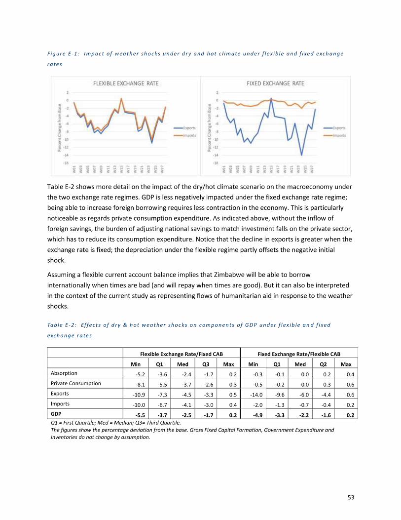
53
Figure E -1 : I mpac t of wea ther sh ocks under d ry and hot c l i mate under f lex ib le and f i xed exchange
rates
Table E-2 shows more detail on the impact of the dry/hot climate scenario on the macroeconomy under
the two exchange rate regimes. GDP is less negatively impacted under the fixed exchange rate regime;
being able to increase foreign borrowing requires less contraction in the economy. This is particularly
noticeable as regards private consumption expenditure. As indicated above, without the inflow of
foreign savings, the burden of adjusting national savings to match investment falls on the private sector,
which has to reduce its consumption expenditure. Notice that the decline in exports is greater when the
exchange rate is fixed; the depreciation under the flexible regime partly offsets the negative initial
shock.
Assuming a flexible current account balance implies that Zimbabwe will be able to borrow
internationally when times are bad (and will repay when times are good). But it can also be interpreted
in the context of the current study as representing flows of humanitarian aid in response to the weather
shocks.
Tab le E -2: Ef fe ct s of d ry & h ot wea ther shoc ks on comp onents of GDP under f lex ib le an d f i xed
exchange ra te s
Flexible Exchange Rate/Fixed CAB Fixed Exchange Rate/Flexible CAB
Min Q1 Med Q3 Max Min Q1 Med Q2 Max
Absorption -5.2 -3.6 -2.4 -1.7 0.2 -0.3 -0.1 0.0 0.2 0.4
Private Consumption -8.1 -5.5 -3.7 -2.6 0.3 -0.5 -0.2 0.0 0.3 0.6
Exports -10.9 -7.3 -4.5 -3.3 0.5 -14.0 -9.6 -6.0 -4.4 0.6
Imports -10.0 -6.7 -4.1 -3.0 0.4 -2.0 -1.3 -0.7 -0.4 0.2
GDP -5.5 -3.7 -2.5 -1.7 0.2 -4.9 -3.3 -2.2 -1.6 0.2
Q1 = First Quartile; Med = Median; Q3= Third Quartile. The figures show the percentage deviation from the base. Gross Fixed Capital Formation, Government Expenditure and Inventories do not change by assumption.

54
Appendix F. Development of Investment Packages and Integration into CGE
F.1 Development of Packages
The development of investment packages presented here uses cost figures for research and development taken
from a previous World Bank study for Europe and Central Asia. Instituting a research and development program in
Zimbabwe may be more or less expensive than doing so in Europe and Central Asia, however, no more obviously
applicable costs estimates were readily available within Africa. This source of uncertainty should be noted when
interpreting the quantitative results presented in this report.
Irrigation systems. This investment involves developing approximately 67,000 additional hectares of
irrigated land at a capital cost of $480 million, with an even mix of new and rehabilitated irrigation
systems. Capital costs for these systems were drawn from Dzingirai et al. (2014), who indicate that new
sprinkler systems cost $8500/ha and rehabilitated systems are $3000/ha. In addition, the costs of
providing a fixed quantity of upstream storage are also added to the totals. These irrigation system costs
only include hard infrastructure investment, covering field and conveyance infrastructure and water
storage, but do not include other soft investment requirements such as water management extension
services etc. Note that the necessary investment for the irrigation adaptation option looks expensive relative to
the second option described below. However, investment in irrigation would create jobs and economic spillovers
during construction of canals etc. While this study does not capture these impacts, this is an area to keep in mind
for future enhancements to this work.
Improved crop varieties and increased inputs. This investment is planned for 56,000 hectares, but at
the much lower initial investment cost of $22 million. Annual costs of this intervention are
proportionately much higher (for fertilizer and seed purchases), at $11 million per year. To illustrate the
potential resources needed to develop improved crop varieties that are tailored to local conditions,
costs were adopted from a World Bank study of climate change adaptation in Eastern Europe and
Central Asia (Sutton et al. 2013). In this study, capital and O&M costs of developing an agricultural
research and development center were estimated based on World Bank Project Appraisal Documents
(PADs) from countries in the region, averaged to a per hectare level, and then compared to the farm
revenue gains from higher performing varieties. This current study applies a similar approach to provide
indicative potential returns of such a program in Zimbabwe. For fertilizer costs, according to FAO
(2006), average application rates of fertilizer for the LSCF farms were 290 kg/ha when the study was
conducted, whereas on communal and SSC farms, rates were 15 kg/ha and 33 kg/ha respectively.18 The
analysis assumes that current application of fertilizer on the three farm types is 30 kg/ha, and that this
18 Note that the authors acknowledge these estimates of LSCF application rates may be higher than current levels for a number of reasons related to land reform.

55
increases to approximately 240 kg/ha (for groundnuts, see the example below) to realize the modeled
yield improvements in AquaCrop. Costs per year for the additional fertilizer were $126/ha, with prices
taken from local sources. For example, in 2015, two of the most common fertilizers, compound D and
AN, were $0.55/kg and $0.62/kg respectively, according to local newspaper articles (e.g.,
http://www.herald.co.zw/fertiliser-prices-drop-again/). Note that the fertilizer application from local
sources has been severely constrained in recent years, and that increasingly farmers have been relying
on imports.
F.2 Treatment of Investment Scenario Costs in the CGE
One adaptation option for drier futures is to invest in irrigation. We explore this in the modelling. It is
useful to think intuitively about likely impacts, to help design the modelling strategy.
An intuitive account
The benefits from irrigation are reasonably clear. It will raise productivity in the irrigated activities in the
absence of CC and will reduce negative impacts of CC induced weather shocks when they do occur.
These positive impacts will have positive spillovers to the rest of the economy.
Other direct impacts anticipated could include the injection of demand while the irrigation
infrastructure is being built, through a standard investment multiplier process. Typically, these benefits
are claimed when large investment projects are proposed. However, the effect will depend on whether
the irrigation investment represents additional investment in the economy or whether it displaces other
investment that would have taken place. With Zimbabwe’s tight current account constraint, it is likely
that the latter will be the case. From a modelling perspective we think it is better to assume the latter,
since we focus on the irrigation investment as such and not on the injection of new investment.
The costs are less obvious. The direct costs will be building the irrigation infrastructure and operational
costs for running irrigated farms. But there will also be indirect costs, primarily the opportunity costs
associated with investment in irrigation rather than in foregone alternatives. These are particularly
pertinent in Zimbabwe as it attempts to rebuild its economy.
If we were comparing the irrigation project with a specific alternative—say improving transport
infrastructure—we could compare internal rates of return, appropriately estimated to capture social as
well as private returns. However, that is not the case in this study. The investment resources for
irrigation do not result in a reduction of investment in one specific sector, but rather from all sectors.
The impact on any specific sector is relatively small.
Investment in irrigation competes with other investment not only through the macroeconomic channel,
which requires aggregate savings and investment to be equal, but also through microeconomic
channels. The irrigation investment requires cement. That must be provided from local suppliers or
through imports. If local cement capacity is limited, there could be a price rise, affecting all other users
of cement. If the cement is imported, there could be exchange rate depreciation, affecting other users
of foreign exchange.

56
In an economy-wide setting, savings—the source of investment resources—may be endogenous to the
pattern of investment. It is possible that investment in irrigation generates slower output (and income)
growth than investment elsewhere. If savings depend on income, the reduced savings reduces
investment in the future, inducing a vicious circle.
Investments typically have a build phase before the additional capacity created comes into operation.
Resources are thus used before output rises. The length of the build phase will vary across sectors and
projects; building a large dam and extensive irrigation canals will likely take longer than expanding
capacity in a textile factory. The phasing in of the additional capacity will also depend on the nature of
the project. If the investment is truly lumpy and must be fully completed before it can be used, there
could be a significant delay before the output and productivity enhancing effects come into play. Thus,
completing a large dam will have little effect on agricultural output before completion, while small dams
with localised irrigation might be brought on stream in small doses, raising productivity, before the
complete project is finished.
The immediate impact of the irrigation investment will thus depend on its profile and on the output-
reducing effects of crowding out investment from other destinations.
All investment ultimately raises capacity in the economy. However, infrastructure investment works
slightly differently from private investment. The latter raises output directly by raising capacity. The
former affects output more indirectly through its impact on productivity of sectors using the
infrastructure. Its impact on output and growth therefore depends on the response of the sectors
intended to benefit from it.
Modelling strategy
With these preliminaries out of the way, we discuss the modelling strategy adopted.
The biophysical modelling gives us three sets of data.
• The estimate of capital costs of the irrigation required to achieve these productivity off-sets in
each crop;
• The impact of irrigation on yields of crops/farm types in 2030 under the different climate
scenarios. Not all crops or farm types are affected;
• The estimated annual operating costs associated with the irrigation.
Ideally, we would like to explore these in a dynamic model, with irrigation taking place, and having
productivity enhancing effects, over time. However, as explained elsewhere, we did not use the dynamic
model to examine CC effects, since we are unable to compare arrivals of historical and CC-induced
weather shocks. Similarly, we do not know the time profile of the irrigation investment and, more
importantly, the time profile of its impact on agricultural productivity.
Our broad modelling strategy therefore was to use the dynamic model to generate a new hypothetical
economy for 2030, assuming investment in irrigation takes place before 2030. We then used this new

57
economy to compare the with-irrigation climate productivity shocks for 2030 with the outcomes under
the no-irrigation shocks we ran previously.
We explored alternative profiles of the irrigation investment: spread over each year between 2020 and
2029, bunched towards the beginning or towards the end of the period. None of these had a significant
impact on the hypothetical 2030 economy generated. Indeed the 2030 with investment economy
generated was never significantly different from the previous hypothetical economies. (We tested the
SAM by calculating multipliers, which were essentially the same).
We therefore dropped the modelling of the investment.
The insignificant impact of the irrigation investment in the model is driven by two assumptions. Firstly,
there are no additional resources for investment via foreign savings: aggregate investment does not rise.
Secondly, although the irrigation investment reduces investment elsewhere, it is not taken away from
any one destination but spread over all sectors. Its impact on any single sector is thus small and the
capital structure in 2030 is unaffected.
We think these assumptions are a reasonable reflection of what is likely to be the case in reality. If there
is significant donor support for irrigation in the future, its impact will be because of the inflow of foreign
resources, not because they flow into irrigation. In addition, we think the nature of irrigation investment
is such that it can be rolled out in small instalments, avoiding some of the problems associated with
lumpiness discussed above.

58
Appendix G. Implementation of Adaptation Investments in the CGE Model
Each adaptation investment has three aspects:
• the impact of the intervention on crop yields;
• the annual operational cost of the intervention; and
• the capital cost of the intervention.
It is useful to look at the gross benefits of the intervention—the impacts arising from the positive
impacts of the intervention on crop yields—and the net benefits—the gross benefits less the annual
operational costs.
There are thus three sub-scenarios for each of the three climate scenarios: without intervention, gross
intervention impacts and net intervention impacts. For each, we can also distinguish, as noted above,
between fixed and flexible exchange rates. Although we ran all these through our model, we cannot
report all the results, nor is it useful to do so. Rather, we want to extract some general lessons, using the
modelling scenarios to both to guide and illustrate our interpretation.
Although they differ in magnitude and sign, all of the initial shocks are of the same type: yields of certain
crops increase or fall. It is useful to have some idea of how these changes work in principle. We use
maize and the dry and hot climate scenario to illustrate, since these have some significant impacts.
Say a negative weather shock reduces maize yields and, other things equal, output. Since the weather
shock does not directly reduce the demand for maize, the price of maize will rise.19 There is thus an
incentive to supply more maize. The additional supply can come from increased production or from
reduced net exports—switching from exports to the domestic market and/or importing. To the extent
that the latter cannot completely compensate for the fall in output, there is an incentive for domestic
producers to off-set the negative yields shock by increasing inputs into maize production. There might
be a change in material inputs, such as fertilizer, or in primary inputs, such as labour, capital and—
importantly—land. There is thus what seems to be a perverse response: declining productivity leads to
maize attracting more rather than less resources.20 We might assume that falling yields will discourage
producers, but that ignores the compensating price effects.
19 In basic economic terms, the negative yield shock shifts the supply curve to the left. 20 Notice that there is a difference between a negative weather shock under historical weather patterns and under
a climate scenario. In the former case, producers know that there are weather variations and it is only after the land has been planted that it is known to be a bad season. With knowledge that climate is changing, the arrival of a bad weather can change expectations—this is the new normal—and therefore behaviour. We should ideally use a dynamic model to explore this. Although we do not do so here, the static model results can be interpreted as long run outcomes.
59
In our modelling we focus on the weather under different climate scenarios for a single year. However,
over time the dry and hot climate scenario implies a declining yield; the drop is not a one-off drop but a
deterioration. In this case, the result we find here implies that resources shift into a sector with declining
productivity. This is the opposite of what a developing country should be doing. We want resources to
shift into sectors with high and growing productivity. Although the response is rational from the point of
view of the individual farmers it may not be socially optimal.
As noted above this effect on domestic resource allocation can be offset by declining net exports. The
space for this to happen will vary from sector to sector. Zimbabwe does not export a great deal of its
maize crop, limiting the potential for export switching. The possibility of raising imports is not limited by
the initial share of imports (about 14% in the integrated economy in 2030) but rather by policy. Since
the climate shock hits local producers there may be calls for them to be protected from imports; such a
response would exacerbate the sub-optimal resource shifts we describe above.
Finally, the process we have described could be affected by what happens globally. Although
Zimbabwe’s maize yields might fall, they may fall more in relevant foreign producers. Zimbabwe’s
competitive advantage could rise.
The dualistic nature of Zimbabwe’s agriculture adds a further dimension to the above. The yield shocks
differ across the two farm types, since they use different technologies. In addition, the responses differ
since they are constrained in different ways. The shocks therefore have distributional consequences.
The above general arguments focus on the sectors directly affected by the climate. They apply to all
sectors receiving negative shocks, but obviously vary with the precise features of the sectors.
Example: Irrigation Investment
One adaptation option for drier futures is to invest in irrigation infrastructure to store water and to
supply it to where and when it is needed. We consider such an option in this section. We begin with
observations about investment in general, to set the stage for the more detailed investigation in the
modelling scenarios.
Investments have a build phase before the additional capacity created comes into operation. Resources
are thus used before output rises. The build phase will vary across sectors and projects—building a dam
will likely take longer than expanding capacity in a textile factory. The phasing in of the additional
capacity will also depend on the nature of the project. Completing a large dam will have little effect on
agricultural output until the irrigation structures have been completed. However, small dams with
localised irrigation, might be brought on stream, raising productivity, before the complete project is
finished.
The impact of the investment in irrigation will depend crucially on how the investment is
accommodated. If the investment envelope is constrained because savings cannot be raised, resources
will be channelled away from other investments, reducing growth in other sectors. The crucial question
is whether the investment in irrigation induces the higher savings necessary to accommodate it.
We can construct plausible stories why it might.

60
• If the irrigation project is part of a donor package, foreign savings will rise (the current account
balance will worsen). This might be at the expense of rising debt.
• Domestic savings might also rise. In Zimbabwe’s current economic situation with high
unemployment, it might be thought that an injection of investment demand will have a
multiplier effect, so that GDP and savings rise. However, Zimbabwe’s growth is not constrained
by inadequate labour supplies, but by capacity, foreign exchange, credit and so on. It is
therefore unlikely that the irrigation investment will create a growth spurt that allows either
private savings to rise because of higher incomes or public savings to rise because of higher
revenue.
In the modelled scenarios, we assume that total investment is fixed so that investment in irrigation
means reduced investment in other sectors. While donor support for irrigation may be forthcoming, we
feel it is not the relevant option to consider at this stage. It is trivial to argue that increasing investment
by raising foreign savings imposes no opportunity cost on the economy: if donors are willing to build for
us, we can freely spend our income on other things. But the initial question for policy makers should be
what the implications of the scheme are if Zimbabwe supplies all the resources itself. There are
competing demands for investment in Zimbabwe, especially as it attempts to reconstruct the economy,
so channeling investment into irrigation has opportunity costs in the form of foregone investment
elsewhere.21
Investment in irrigation competes with other investment not only through the macroeconomic channel,
which requires aggregate savings and investment to be equal, but also through microeconomic
channels. The irrigation investment requires cement. That must be provided from local suppliers or
through imports. If local cement capacity is limited, there could be a price rise, affecting all other users
of cement. If the cement is imported, there could be exchange rate depreciation, affecting other users
of foreign exchange.
All investment ultimately raises capacity in the economy. However, infrastructure investment works
slightly differently from private investment. The latter raises output directly by raising capacity. The
former affects output more indirectly through its impact on productivity of sectors using the
infrastructure. Its impact on output and growth therefore depends on the response of the sectors
intended to benefit from it.
With these preliminaries out of the way, we discuss the modelling strategy
The biophysical modelling has given us three sets of data.
21 If donors are willing to provide the resources for massive irrigation investment—presumably on the presumption that it will benefit Zimbabweans, one should consider whether similar support for investment elsewhere might not have even more beneficial impacts. Of course, if Zimbabwe does not reduce its own investment because of the donor support, the principle of fungibility suggests the donors are supporting the least productive investment undertaken.

61
• The estimate of capital costs of the irrigation required to achieve these productivity off-sets in
each crop;
• The impact of irrigation on yields of crops/farm types under the different climate scenarios. Not
all crops or farm types are affected; and
• The estimated annual operating costs associated with the irrigation.
Our broad modelling strategy is to assume that the investments are made before 2030 and then
compare the with-irrigation climate productivity shocks for 2030 with the outcomes under the no-
irrigation shocks we ran previously. To do this we have to run a dynamic model to create a new
hypothetical SAM representing the economy in 2030 after the irrigation investment has occurred.
The costs of the irrigation, and its impact on crops were estimated by the biophysical modellers and are
discussed elsewhere.
The capital costs relate to the total cost of irrigation. In aggregate they constitute about 27% of Gross
Fixed Capital Formation in 2013. While we would not expect this investment to take place in one year,
we do not have a profile for how it might be spread out. We assume that the whole project takes five
years, starting in 2023. We also assume that no benefits flow from the investment until after it is
completed. Agricultural productivity is unaffected until it is completed.
In addition to the capital costs, irrigation imposes operational costs on the irrigated crop producers.
Their costs of production rise as a direct consequence of the irrigation, as they incur maintenance and
replacement costs. The estimates of these amount to about 6.0% of the gross value of output of the
irrigated crops in 2013. To model these we need to make some assumptions about how they are
accommodated in the cost structures of the crop producers.
Ultimately, the O&M costs are integrated into the CGE analysis, but integrating the capital costs would
require a dynamic model with impact shocks over time.

62
Appendix H. Results of Engineering Cost Analysis
H.1 Impacts on Farm Revenues
This section presents the economic findings of the study from an “engineering cost” perspective, where
impacts of climate change and benefits of adaptation are measured by simply multiplying changes in
yields by the static 2030 forecast crop prices described in Table A-3.
In terms of economic impacts, total average baseline agricultural revenues for the 13 crops considered
in this study are estimated at approximately $1 billion annually, based on the production estimates from
ZimStat and the prices described in Table A-3. This estimate falls roughly within the expected range –
the gross income from agriculture in Zimbabwe in 2014 was approximately $1.5 billion, of which $760
million was from field crops (USDA 2015).
Table G-1 shows the impacts of climate change on crop revenues, broken down across farm types and
climate scenarios. The overall economic effects of climate change range from an annual loss of $186
million under the dry/hot scenario, to a gain of $129 million under the wettest scenario – this is
between a 15% loss and 11% gain in total revenues. The communal farm types, which support by far the
largest number of livelihoods, are projected to experience the largest reductions (and gains) in
revenues. On the other hand, the LSCF farm types experience almost no downside risk because of their
relatively high dependence on irrigation – in the dry/hot scenario, any reduced rainfed yields are offset
by beneficial temperature effects.22
Tab le G - 1: Impa ct o f c l im ate change on average annua l cr op re v enues by farm type
Farm Type Control
Revenues
Climate Scenario
Dry/Hot Medium Wettest
LSCF $427.1 ($0.9) $3.3 $26.5
A2 $233.2 ($35.7) ($16.1) $26.4
A1 $136.6 ($36.6) ($16.8) $19.5
Communal $330.3 ($89.7) ($39.7) $44.4
SSC $17.8 ($4.6) ($2.4) $2.4
Old Resettle $77.3 ($18.2) ($10.8) $9.3
TOTAL $1,222 ($185.8) ($82.4) $128.5
Change -15% -7% 11%
22 This is not to suggest that no LSCF farmers would be negatively affected by climate change, but rather that on average, the effects are generally positive.

63
Table G-2 presents these effects across the different AERs. AER 2 is shown to have the highest impacts,
both losses and gains and positive. AER 5 shows limited negative impacts because a large fraction of
these revenues are from irrigated sugarcane, which are protected from water stress impacts by
assumption. As noted above, water for irrigation could certainly be limited under a dry climate change
future.
Tab le G - 2: Impa ct o f c l im ate change on average annua l cr op re venues by AER
AER Control
Revenues
Climate Scenario
Dry/Hot Medium Wettest
1 $17.6 ($4.0) ($2.8) $0.8
2 $422.5 ($90.3) ($51.2) $49.4
3 $146.7 ($47.0) ($19.7) $22.2
4 $144.8 ($42.9) ($16.4) $22.8
5 $490.6 ($1.5) $7.7 $33.4
TOTAL $1,222 ($185.8) ($82.4) $128.5
Change -15% -7% 11%
H.2 Benefits from Adaptation
We next ask how adaptation can improve this situation. The remainder of this Appendix examines this
question from an engineering cost perspective, whereas Chapter 4.2 considers this question using
general equilibrium model outcomes. The agricultural sector adaptation analysis considers two options
and one baseline “no adaptation” option to illustrate how damages under the drier scenarios could be
reduced. Several general assumptions are central to this analysis. Because this is an analysis of
conditions in 2030 under 28 different possible weather outcomes, capital costs of investments are
annualized to 2030 based on assumed infrastructure lifespans and at a discount rate of 5% based on
earlier work conducted with the World Bank. O&M costs are also included in the analysis, and are
documented in the individual sections on adaptation options below.
H.2.1 Adaptation Option 1: Irrigation
Irrigation can enhance yields by reducing water stress, which is particularly important in the drier
regions of Zimbabwe. Two alternatives were considered – construction of new irrigation systems, and
rehabilitation of the many dilapidated systems that are in place. Capital costs for new and rehabilitated
systems are reported in Section 3.3.2, and incorporate an assumed volume of storage per hectare.
Error! Reference source not found. shows the B-C ratios for these investments on maize and tobacco
farms, with benefits being the average increase in revenues from irrigating (i.e., irrigated minus rainfed
revenues) in 2030, and costs the annualized stream of capital and O&M expenditures in 2030. Maize
and tobacco are two of the crops that receive the highest level of returns on irrigation and thus the
highest amounts of investment. Note that tobacco represented approximately 5% of Zimbabwe’s 2013
GDP, so is an important crop for the economy.

64
Tab le G - 3: Benef i t - cost rat i os for new and rehab i l i ta ted i r r igat i on sy ste m s ac ros s farm types and
AERs, ma ize , 2 03 0
Maize Tobacco
Farm Type
New Irrigation Rehabilitated Irrigation New Irrigation Rehabilitated Irrigation
AER
Base
Dry/H
ot
Me
diu
m
We
ttest
Base
Dry/H
ot
Me
diu
m
We
ttest
Base
Dry/H
ot
Me
diu
m
We
ttest
Base
Dry/H
ot
Me
diu
m
We
ttest
LSCF
1 2.01 2.74 2.49 1.77 3.98 5.44 4.93 3.52 0.33 0.4 0.39 0.28 0.65 0.8 0.78 0.55
2 1 1.5 1.21 0.67 1.98 2.96 2.39 1.33 1.06 1.41 1.41 0.66 2.11 2.79 2.8 1.31
3 0.6 0.77 0.67 0.51 1.19 1.52 1.32 1.01 1.11 1.27 1.21 0.88 2.2 2.52 2.39 1.75
4 0.68 0.81 0.74 0.6 1.34 1.61 1.47 1.18 2.67 2.93 2.87 2.2 5.29 5.8 5.69 4.36
5 1.16 1.26 1.19 1.06 2.3 2.5 2.35 2.1 NA NA NA NA NA NA NA NA
A2
1 0.31 0.42 0.39 0.28 0.62 0.84 0.77 0.56 1.28 1.6 1.54 1.09 2.55 3.17 3.05 2.16
2 0.57 0.85 0.69 0.38 1.13 1.69 1.36 0.76 0.99 1.29 1.23 0.65 1.97 2.57 2.43 1.3
3 0.8 1.02 0.89 0.68 1.59 2.03 1.77 1.35 2.29 2.61 2.49 1.82 4.54 5.18 4.93 3.6
4 0.6 0.71 0.65 0.54 1.19 1.41 1.28 1.07 NA NA NA NA NA NA NA NA
5 0.3 0.32 0.3 0.27 0.59 0.64 0.6 0.53 NA NA NA NA NA NA NA NA
A1
1 0.33 0.44 0.4 0.29 0.65 0.88 0.8 0.57 1.39 1.73 1.67 1.18 2.76 3.44 3.31 2.34
2 0.34 0.51 0.41 0.23 0.67 1 0.81 0.45 0.77 1.01 0.96 0.51 1.53 2 1.89 1.01
3 0.56 0.71 0.61 0.48 1.1 1.4 1.21 0.95 1.36 1.55 1.47 1.08 2.69 3.07 2.92 2.13
4 0.38 0.45 0.41 0.34 0.76 0.9 0.82 0.68 2.38 2.61 2.54 1.98 4.71 5.17 5.03 3.93
5 0.15 0.16 0.15 0.13 0.29 0.32 0.3 0.27 0.32 0.34 0.33 0.27 0.63 0.67 0.65 0.54
Comm
1 0.38 0.46 0.45 0.35 0.75 0.92 0.9 0.7 1.32 1.64 1.58 1.12 2.61 3.25 3.13 2.21
2 0.16 0.24 0.21 0.11 0.31 0.48 0.42 0.22 0.77 1 0.95 0.51 1.52 1.99 1.88 1
3 0.31 0.39 0.35 0.26 0.61 0.77 0.69 0.52 1.8 2.05 1.95 1.42 3.56 4.06 3.87 2.83
4 0.22 0.27 0.25 0.2 0.44 0.53 0.49 0.39 1.07 1.17 1.13 0.9 2.11 2.32 2.24 1.78
5 0.19 0.21 0.2 0.18 0.39 0.42 0.4 0.35 2.38 2.55 2.45 2.02 4.73 5.05 4.85 4.01
SCC
1 0.14 0.17 0.17 0.13 0.28 0.35 0.34 0.26 NA NA NA NA NA NA NA NA
2 0.12 0.18 0.16 0.08 0.23 0.36 0.32 0.17 0.72 0.94 0.89 0.48 1.43 1.87 1.77 0.94
3 0.36 0.45 0.4 0.3 0.71 0.89 0.8 0.6 1.79 2.04 1.94 1.42 3.54 4.04 3.85 2.81
4 0.22 0.26 0.24 0.19 0.43 0.52 0.49 0.38 1.3 1.43 1.4 1.05 2.57 2.83 2.77 2.09
5 0.07 0.07 0.07 0.06 0.13 0.15 0.14 0.12 NA NA NA NA NA NA NA NA
Old Settle
1 0.24 0.29 0.28 0.22 0.47 0.57 0.56 0.44 1.5 1.86 1.79 1.27 2.96 3.7 3.56 2.52
2 0.2 0.31 0.27 0.15 0.4 0.62 0.54 0.29 0.35 0.47 0.49 0.23 0.7 0.94 0.97 0.46
3 0.33 0.42 0.37 0.28 0.66 0.83 0.74 0.56 0.92 1.07 1.04 0.71 1.82 2.12 2.05 1.4
4 0.18 0.21 0.2 0.16 0.35 0.42 0.39 0.31 1.76 1.94 1.9 1.43 3.49 3.84 3.76 2.84
5 0.26 0.29 0.28 0.24 0.52 0.58 0.55 0.48 NA NA NA NA NA NA NA NA
Generally, tobacco responds more positively to irrigation than maize, except in some AERs for the LSCF
farm type. The benefits of irrigation for maize are largely below one for all small holder farm types

65
(owing to lower starting yields and prices), whereas benefits for tobacco are generally high for all farm
types. Not surprisingly, rehabilitated irrigation has higher B-C ratios than construction of new systems
because of the lower capital costs.
H.2.2 Adaptation Option 2: Improved Crop Variety and Increased Inputs
Unlike irrigation, this adaptation option focuses on communal, SCC, and old resettlement farm types.
For instance, Table G-4 shows B-C ratios for improved variety and increased fertilizer application to
groundnuts. Enhancing crop variety adaptation to drier and hotter climates also stands to improve the
resilience of farming systems to climate change. The modeled higher performing varieties in AquaCrop
proportionately increase yields, such that under wetter scenarios yields increase more in absolute terms
than in drier conditions. Fertilizer application has a similar effect: under rainfed conditions, net benefits
tend to be highest in the wetter scenarios, as increased application also increases crop water demands.
Tab le G - 4: Benef i t - cost rat i os for increa sed fer t i l i ze r app l ica t i on a cross far m t ypes and AER s,
g roundnuts , 20 30.
Farm Type
Rainfed Irrigated
AER
Base
Dry/H
ot
Me
diu
m
We
ttest
Base
Dry/H
ot
Me
diu
m
We
ttest
Comm
1 2.92 2.43 2.64 2.81 2.59 2.51 2.51 2.51
2 2.59 1.99 2.43 2.61 2.84 2.84 2.84 2.84
3 1.72 1.1 1.57 1.75 2.26 2.24 2.24 2.24
4 1.31 0.9 1.2 1.38 1.83 1.81 1.82 1.81
5 0.43 0.23 0.35 0.49 1.35 1.31 1.3 1.3
SCC
1 1.26 1.03 1.13 1.2 1.07 1.04 1.04 1.04
2 2.04 1.37 1.91 2.03 2.66 2.65 2.65 2.65
3 2.8 1.91 2.56 2.86 3.47 3.44 3.44 3.44
4 1.17 0.81 1.06 1.23 1.62 1.61 1.61 1.61
5 0.53 0.29 0.44 0.59 1.39 1.34 1.33 1.34
Old Settle
1 NA NA NA NA NA NA NA NA
2 3.25 2.5 3.05 3.28 3.57 3.56 3.56 3.56
3 1.96 1.33 1.78 2 2.42 2.4 2.4 2.4
4 1.17 0.81 1.06 1.23 1.62 1.61 1.61 1.61
5 1.51 0.82 1.24 1.67 4.01 3.88 3.85 3.86

66
Appendix I. Study Caveats and Recommended Further Analysis
I.1 Study Caveats
This study is subject to several key sources of uncertainty, some of which are partly addressed in the
analytical design (climate projections) and others that are well outside of the scope of this study (e.g.,
geopolitical uncertainty).
Uncertainty in climatic projections. Taking the Zambezi River basin as an example, climate projections
obtained from the GCMs reflect deep uncertainty as illustrated by the Climate Moisture Index (CMI) in
Figure H-1. CMI is a measure of aridity in the region and the green and blue dots corresponding to the
Zambezi display the uncertainty in the results spectrum obtained from Coupled Model Intercomparison
Project phase 3 (CMIP3) and phase 5 (CMIP5) suite of models. Hence, it is of paramount importance to
consider this inherent climate uncertainty while formulating agricultural response strategies (Boehlert et
al. 2015, Strzepek et al. 2013).
Figure H -1 : C l i mate chang e proj ec t i ons acr oss Afr ica ’ s r i ver bas ins
Note: The CMI combines the effect of rainfall and temperature projections. The index values vary between −1 and +1, with lower values representing more arid conditions. The chart reports CMI values (averaged over the period 2010–50) projected by climate models included in the CMIP3 and CMIP5 ensembles. In each basin, the red dot denotes the average value of CMI in the historical baseline. Dots to the right of the historical value refer to projections of wetter climate; dots to the left indicate projections of drier climate. Source: Cervigni et al. (2015).

67
Water availability for irrigation. This study evaluates the full impacts of climate change on rainfed
agriculture and the temperature effects on irrigated agriculture, but does not analyze the impact on
irrigation water availability or the resulting effects on irrigated crop yields. Under a dry/hot scenario,
water availability will fall and irrigation water requirements will rise, creating the potential for large
increases in unmet irrigation water demand and increasing levels of pressure on already falling
groundwater supplies. This will have a potentially significant effect on Zimbabwe’s economy, but to
properly project unmet irrigation water requirements would require a water systems model that was
unavailable for this study. Cervigni et al. (2015) applied such a model to evaluate irrigation water
availability in the Zambezi, and found that large increases in unmet demand would occur under many of
the climate scenarios considered (Figure H-2).
Figure H -2 : Change in unmet i r r iga t i on wa ter de ma nd and hydro power genera t i on in the Za mbez i
Bas in under 12 1 future c l i mate s , re lat i ve to h i stor ic a l cond it i ons
Source: Cervigni et al. 2015
Effects of climate change on pest behaviour. Climate change can also affect agricultural output by
changing pest behaviour. The rapid spread of fall army worm from the Americas to Africa is probably
driven by climate change. Its impact is already substantial and could potentially be devastating. Since it
appears to be most destructive in rainy periods immediately following a drought, it could reduce the
potential for recovery from severe drought periods. We have not modelled this.
Effect of irrigation investments on crop mix. This study assumes that specific crops, such as maize, are
grown in areas where irrigation investments occur. Once irrigation is available, farmers may instead

68
shift to higher value cash crops. This would have the effect of reducing food self-sufficiency but
potentially increasing the economic returns from the agricultural sector.
Global macroeconomic effects. Climate change will also affect Zimbabwe because of impacts elsewhere
in the world. Global commodity prices can change because of impacts far away. Oil prices can change
because of policy decisions taken elsewhere. While Zimbabwe has little influence on these, they can
impact the Zimbabwean economy. These impacts should be considered when designing responses.
Investing in irrigation for a particular crop, which is anticipated to become harder to produce in
Zimbabwe, makes more sense if its global price is more likely to rise than fall.
I.2 Recommended Further Analysis
As suggested above, a more comprehensive study would be needed to confirm these findings and
evaluate a broader range of adaptation options, most notably examining the behavioural response to
climate change both at the individual farm and national level, including crop switching as an adaptation
option and in response to improved production possibilities offered by irrigation. Until this proposed
extension, the GDP effects presented above are likely to be under-estimated for irrigation, especially
under the dry/hot scenario for smallholder agriculture.
This study is a first step in trying to understand the effects of climate change on Zimbabwe’s agricultural
sector and economy. Such efforts must be ongoing, with analyses updated and refined as better
information and analytical methods become available. For instance, one such area of new insights is the
growing acceptance that forests can play an important role for watershed protection and achieve better
irrigation outcomes, while supporting income diversification. A study commissioned to investigate the
benefits of more effective catchment and forest management on the agricultural sector would help to
justify making these investments. Such a study would evaluate how changes in land use and
management affect the variability of downstream water availability and likelihood of extreme events,
using software such as the Soil Water Assessment Tool (SWAT).
On the biophysical side, a Zimbabwe-wide water balance model would allow for evaluation of unmet
demand for irrigation water, which is a critical risk under climate change. The ongoing drafting of the
National Water Resources Master Plan is a significant undertaking in this direction. Energy-water
linkages are also central, as much irrigation requires electricity for groundwater pumping or
pressurization and a dry climate future will threaten watersheds and hydroelectric reservoirs thereby
driving electricity prices up. Evaluating these interlinked and varied effects in an integrated framework
is important and should be undertaken in the future. Additionally, future unmet water demand could
also potentially be damped through water pricing, with the understanding that this would require the
implementation of a system of metering and policies that are currently not in place.
Furthermore, this study considers only two sample adaptation options out of many possible others. It is
recommended that a more comprehensive adaptation study be conducted to investigate a much

69
broader range of options, including ecosystem based approaches, crop switching and risk management,
as informed by stakeholder preferences. In addition to future work evaluating a more comprehensive
menu of adaptation options, it would also be helpful to consider different possible options in
conjunction with each other, grouped into a variety of different adaptation packages.
The economy-wide model itself could also be enhanced. First, this analysis does not integrate the
investment costs into the economy over time. Doing so would allow a more thorough evaluation of the
net effects of these investments, and of the opportunity costs relative to potentially higher return
alternatives. One of these alternatives may be a more significant investment in the manufacturing
sector, which could help to avoid the middle income trap as Zimbabwe continues to develop. Next, this
study evaluates aggregate GDP effects, but the government should also take into effect distributional
effects across income category, urban/rural, across genders and others. This would require that
enhanced demographic and economic data be input into the SAM used in this study. Additionally, this
report has not taken into account the regional dimension of climate change impacts on agriculture: it
has not considered migration, or proactively shifting crops into higher altitude areas as temperature
rises. Finally, future work could examine adaptation options for agriculture through the lens of existing
national, sub-national and regional policies and with international commitments in mind.

70
Appendix J. Macroeconomic Effects
Macroeconomic effects: These depend on the mechanisms that constrain adjustment in the economy
(‘closure rules’). Our model reflects these in three important areas:
a. The Government Budget Balance: We assume that the government budget balance can vary. Thus, if
a fall in GDP causes a fall in government revenue, the government does not reduce its expenditure
but rather allows the budget balance to fall. Similarly for GDP increases. In essence, government
treats both negative and positive weather shocks as temporary and is not credit constrained.
b. The Current Account Balance: We explore alternative adjustment constraints here. We compare the
implications of holding the exchange rate fixed and allowing the current account balance to adjust
against the alternative of holding the current account balance fixed and allowing the exchange rate
to adjust.
c. The Savings and Investment Balance: National accounting consistency requires that aggregate
investment expenditure must equal national savings. We assume that investment expenditure is
determined outside the model and that national savings adjusts to ensure equality.
These three areas interact with each other. National savings comes from domestic private savings by
households and enterprises, from domestic public savings (the government budget balance) and from
foreign savings (the negative of the current account balance):
Investment Private Savings by Government Saving Foreign Savings= Gross Fixed Capital Formation
households and firms = Budget Surplus = - Current Account Balance+ Change in Inventories
p g fI S S S
We assume that investment is exogenous: one or other component of savings has to change to maintain
the SI balance. When we assume foreign savings is fixed, the adjustment has to come through the two
domestic sources of savings. Government savings might change, due to changes in the tax base and
prices, but government does not adjust explicitly to the shock. Any residual difference between
investment and national savings will have to be accommodated by private savings. These will change
because of income and price changes, but it is unlikely these changes will exactly match what is
required. Further changes will have to be induced by changing the savings behaviour of firms and/or
households, so that they save a higher or lower proportion of their income. In this set-up a large part of
the burden of adjustment is placed on households.
This burden on households is reduced when foreign savings is able to adjust (with the exchange rate
fixed), since changes in foreign savings partially supply the change in national savings required to match
aggregate investment expenditure.


