A family of linearizable recurrences with the Laurent property

Submitted exclusively to the London Mathematical Societydoi:10.1112/0000/000000

A family of linearisable recurrences with the Laurent property

A.N.W. Hone and C. Ward

Abstract

We consider a family of nonlinear recurrences with the Laurent property. Although theserecurrences are not generated by mutations in a cluster algebra, they fit within the broaderframework of Laurent phenomenon algebras, as introduced recently by Lam and Pylyavskyy.Furthermore, each member of this family is shown to be linearisable in two different ways, in thesense that its iterates satisfy both a linear relation with constant coefficients and a linear relationwith periodic coefficients. Associated monodromy matrices and first integrals are constructed,and the connection with the dressing chain for Schrodinger operators is also explained.

1. Introduction

A nonlinear recurrence relation is said to possess the Laurent property if all of its iterates areLaurent polynomials in the initial data with integer coefficients. Particular recurrences of theform

xn+Nxn = F (xn+1, . . . , xn+N−1) , (1.1)

with F being a polynomial, first gained wider notice through the article by Gale [10], whichhighlighted the fact that such nonlinear relations can unexpectedly generate integer sequences.The second order recurrence

xn+2xn = x2n+1 + 1 (1.2)

is one of the simplest examples of this type. With the initial values x0 = 1, x1 = 1, this generatesa sequence beginning 1, 1, 2, 5, 13, 34, 89, 233, . . ., and it turns out that xn is an integer for alln, but it is not obvious why this should be so. The fact that (1.2) has the Laurent propertyprovides an explanation: if x0 and x1 are considered as variables, then each xn is an elementof the Laurent polynomial ring Z[x±10 , x±11 ], and so generates an integer when evaluated atx0 = x1 = 1.

One of the motivations behind Fomin and Zelevinksky’s cluster algebras, introduced in [5],was to provide an axiomatic framework for the Laurent property, which arises in many differentareas of mathematics. A cluster is an N -tuple x = (x1, x2, . . . , xN ) which can be mutated indirection j for each choice of j ∈ {1, . . . , N}, to produce a new cluster x′ with componentsx′k = xk for k 6= j and x′j determined by the exchange relation

x′jxj =∏

bij>0

xbiji +

∏bij<0

x−biji (1.3)

for a coefficient-free cluster algebra, where B = (bij) is an associated skew-symmetrizable N ×N integer matrix. There is also an associated operation of matrix mutation, B → B′, the precisedetails of which are not needed here.

In general, sequences of mutations in a cluster algebra do not generate orbits of a fixed map,since the exponents in (1.3) both depend on j and vary under the mutation of the matrix B.

2000 Mathematics Subject Classification 11B37 (primary), 13F60, 37J35 (secondary).

CW was supported by EPSRC studentship EP/P50421X/1.

Page 2 of 14 A.N.W. HONE AND C. WARD

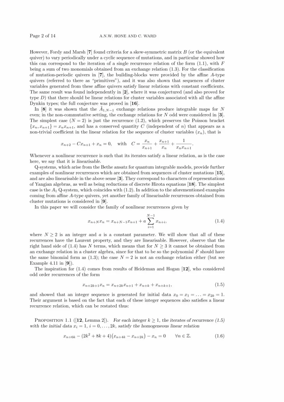
However, Fordy and Marsh [7] found criteria for a skew-symmetric matrix B (or the equivalentquiver) to vary periodically under a cyclic sequence of mutations, and in particular showed howthis can correspond to the iteration of a single recurrence relation of the form (1.1), with Fbeing a sum of two monomials obtained from an exchange relation (1.3). For the classificationof mutation-periodic quivers in [7], the building-blocks were provided by the affine A-typequivers (referred to there as “primitives”), and it was also shown that sequences of clustervariables generated from these affine quivers satisfy linear relations with constant coefficients.The same result was found independently in [2], where it was conjectured (and also proved fortype D) that there should be linear relations for cluster variables associated with all the affineDynkin types; the full conjecture was proved in [16].

In [8] it was shown that the A1,N−1 exchange relations produce integrable maps for Neven; in the non-commutative setting, the exchange relations for N odd were considered in [3].The simplest case (N = 2) is just the recurrence (1.2), which preserves the Poisson bracket{xn, xn+1} = xnxn+1, and has a conserved quantity C (independent of n) that appears as anon-trivial coefficient in the linear relation for the sequence of cluster variables (xn), that is

xn+2 − Cxn+1 + xn = 0, with C =xnxn+1

+xn+1

xn+

1

xnxn+1.

Whenever a nonlinear recurrence is such that its iterates satisfy a linear relation, as is the casehere, we say that it is linearisable.

Q-systems, which arise from the Bethe ansatz for quantum integrable models, provide furtherexamples of nonlinear recurrences which are obtained from sequences of cluster mutations [15],and are also linearisable in the above sense [3]. They correspond to characters of representationsof Yangian algebras, as well as being reductions of discrete Hirota equations [18]. The simplestcase is the A1 Q-system, which coincides with (1.2). In addition to the aforementioned examplescoming from affine A-type quivers, yet another family of linearisable recurrences obtained fromcluster mutations is considered in [9].

In this paper we will consider the family of nonlinear recurrences given by

xn+Nxn = xn+N−1xn+1 + a

N−1∑i=1

xn+i, (1.4)

where N ≥ 2 is an integer and a is a constant parameter. We will show that all of theserecurrences have the Laurent property, and they are linearisable. However, observe that theright hand side of (1.4) has N terms, which means that for N ≥ 3 it cannot be obtained froman exchange relation in a cluster algebra, since for that to be so the polynomial F should havethe same binomial form as (1.3); the case N = 2 is not an exchange relation either (but seeExample 4.11 in [9]).

The inspiration for (1.4) comes from results of Heideman and Hogan [12], who consideredodd order recurrences of the form

xn+2k+1xn = xn+2kxn+1 + xn+k + xn+k+1, (1.5)

and showed that an integer sequence is generated for initial data x0 = x1 = . . . = x2k = 1.Their argument is based on the fact that each of these integer sequences also satisfies a linearrecurrence relation, which can be restated thus:

Proposition 1.1 ([12, Lemma 2]). For each integer k ≥ 1, the iterates of recurrence (1.5)with the initial data xi = 1, i = 0, . . . , 2k, satisfy the homogeneous linear relation

xn+6k − (2k2 + 8k + 4)(xn+4k − xn+2k

)− xn = 0 ∀n ∈ Z. (1.6)

LINEARISABLE RECURRENCES WITH THE LAURENT PROPERTY Page 3 of 14

When N = 3 the recurrence (1.4) coincides with (1.5) for k = 1, and is a special case of amore general third order recurrence that is shown to be linearisable in [14].

In the case of (1.4) it turns out that the integer sequence generated by choosing all N datato take the value 1 is related to the Fibonacci numbers, which we denote by fn (with theconvention that f0 = 0, f1 = 1). The analogue of Proposition 1.1 is as follows.

Proposition 1.2. For each integer N ≥ 2, the iterates of recurrence (1.4) with the initialdata xi = 1, i = 0, . . . , p = N − 1, satisfy the homogeneous linear relation

xn+3p − (f2p+2 + pf2p − f2p−2 + 1)(xn+2p − xn+p

)− xn = 0 ∀n ∈ Z. (1.7)

1.1. Outline of the paper

Although (1.4) cannot be obtained from a cluster algebra, in the next section we brieflyexplain how it fits into the broader framework of Laurent phenomenon algebras (LP algebras),introduced in [17], which immediately shows that the Laurent property holds. In the thirdsection we present Theorem 3.3, our main result on the linearisability of (1.4); in additionto a linear relation with coefficients that are first integrals (i.e. conserved quantities like Cabove), the iterates also satisfy a linear relation with periodic coefficients. Although the resultessentially follows by adapting methods from [9], the complete proof involves the detailedstructure of monodromy matrices associated with an integrable Hamiltonian system, namelythe periodic dressing chain of [20]; this connection is explained in section 4. Section 5 containsour conclusions, while the properties of the particular family of integer sequences in Proposition1.2 are reserved for an appendix.

2. Laurent phenomenon algebras

A seed in a cluster algebra is a pair (x, B), where x is a cluster and B is a skew-symmetrizableinteger matrix; for each index j, an associated exchange polynomial is given by the right handside of (1.3). In the setting of LP algebras, introduced recently by Lam and Pylyavskyy [17],the exchange polynomials are allowed to be irreducible polynomials with an arbitrary numberof terms, rather than just binomials. The Laurent phenomenon for certain recurrences of thetype (1.1) with non-binomial F was already observed in Gale’s article [10], with Fomin andZelevinsky’s Caterpillar Lemma eventually providing a means to prove the Laurent propertyin this more general setting [6]. The axioms of an LP algebra, which we briefly describe below,guarantee that mutations of an initial seed always produce Laurent polynomials in the initialcluster variables.

A seed in an LP algebra of rank N is a pair of N -tuples t = (x,F), where x is acluster, and the entries of F are exchange polynomials Fj ∈ P := S[x1, . . . , xN ], where Sis a coefficient ring. The exchange polynomials must satisfy the conditions that (1) Fj isirreducible in P and not divisible by any variable xi, and (2) Fj does not involve the variablexj , for j = 1, . . . , N . A set of exchange Laurent polynomials {F1, . . . , FN} is also definedsuch that, for all j, (i) there are ai ∈ Z≤0 for each i 6= j with Fj = Fj

∏i6=j x

aii , and (ii)

Fi|xj←Fj/x ∈ S[x±11 , . . . , x±1j−1, x±1, x±1j+1, . . . , x

±1N ] and is not divisible by Fj . Note that here (as

in [6], for instance) we use F |x←g(x,y,...) to denote the result of substituting g(x, y, . . .) for x inF = F (x, y, . . .). Mutation in direction j gives (x,F)→ (x′,F′), where the cluster variables ofthe new seed are given by x′k = xk for k 6= j and x′j = Fj/xj . For the new exchange polynomials,set

Gk = Fk

∣∣∣xj←

Fj |xk←0

x′j


and define Hk by removing all common factors with Fj |xk←0 from Gk; then F ′k = MHk whereM is a Laurent monomial in the new cluster variables. Lam and Pylyavskyy proved in [17,Theorem 5.1] that the Laurent phenomenon holds for LP algebras, which means that clustervariables obtained by arbitrary sequences of mutations belong to S[x±11 , . . . , x±1N ].

To see how each of the recurrences (1.4) fits into the LP algebra framework, we take thecoefficient ring S = Z[a]. The initial seed is then given by t1 = {(x1, F1), . . . , (xN , FN )}, withthe irreducible exchange polynomials

F1 = xNx2 + a

N∑i=2

xi, FN = xN−1x1 + a

N−1∑i=1

xi, Fk = a+ xk−1 + xk+1 otherwise.

Mutating t1 in direction 1 gives a new seed t2 = {(xN+1, F′1), (x2, F

′2), . . . (xN , F

′N )}, containing

one new cluster variable x′1 = xN+1, where

F ′1 = F1, F ′2 = xN+1x3 + a

N+1∑i=3

xi, F ′N = a+ xN−1 + xN+1, F ′k = Fk otherwise.

The seeds t1 and t2 are similar to each other, in the sense of 3.4 in [17] (see also section7 therein): they are transformed one to the other by (x1, x2, . . . , xN )→ (x2, x3, . . . , xN+1),corresponding to a single iteration of (1.4), and successive iterations are generated by mutatingt2 in direction 2, and so forth. For the rest of the paper, it will be more convenient to takex0, x1, . . . , xN−1 as initial data, and introduce the ring of Laurent polynomials

RN := Z[a, x±10 , . . . , x±1N−1],

in order to make the following statement.

Theorem 2.1. For each N the Laurent property holds for (1.4), i.e. xn ∈ RN ∀n ∈ Z.

Working in the ambient field of fractions Q(a, x0, . . . , xN−1), it is also worth noting that,from the form of (1.4), the iterates xn can be written as subtraction-free rational expressionsin a and the initial data, and hence are all non-vanishing.

3. Linearisability

In order to show that the iterates of (1.4) satisfy linear relations, we begin by noting thatthe nonlinear recurrence can be rewritten using a 2× 2 determinant as

Dn = a

N−1∑i=1

xn+i, where Dn :=

∣∣∣∣ xn xn+N−1xn+1 xn+N

∣∣∣∣ , (3.1)

and proceed to consider the 3× 3 matrix

Ψn =

xn xn+N−1 xn+2N−2xn+1 xn+N xn+2N−1xn+2 xn+N+1 xn+2N

. (3.2)

Iterating (1.4) with initial data (x0, x1, . . . , xN−1) is equivalent to iterating the birational map

ϕ : (x0, x1, . . . , xN−1) 7→

(x1, x2, . . . ,

(xN−1x1 + a

N−1∑i=1

)/x0

). (3.3)

The key to obtaining linear relations for the variables xn is the observation that the determinantof the matrix Ψn is invariant under n→ n+ 1, meaning that it provides a conserved quantityfor the map ϕ.


Lemma 3.1. The determinant of the matrix Ψn is invariant under the map ϕ defined bythe recurrence (1.4). In other words, if it is written in terms of the initial data as

det Ψn = µ(x0, x1, . . . , xN−1), (3.4)

then the function µ is a first integral, i.e. it satisfies ϕ∗µ = µ.

Proof. To begin with, we note that the identity

Dn+1 −Dn = a(xn+N − xn+1) (3.5)

follows from (3.1). We wish to show that det Ψn+1 = det Ψn for all n. However, since allformulae remain valid under shifting each of the indices by an arbitrary amount, it is sufficientto perform the calculation with n = 0 for ease of notation. Using the method of Dodgsoncondensation [4] to expand the 3× 3 determinant in terms of 2× 2 minors, we calculate

det Ψ0 =1

xN

∣∣∣∣ D0 DN−1D1 DN

∣∣∣∣ =1

xN

∣∣∣∣ D1 + a(x1 − xN ) DN + a(xN − x2N−1)D1 DN

∣∣∣∣=

a

xN

(DN (x1 − xN )−D1(xN − x2N−1)

),

where we have used (3.5). Similarly, by using (3.5) again, we have

det Ψ1 =1

xN+1

∣∣∣∣ D1 DN

D2 DN+1

∣∣∣∣ =1

xN+1

∣∣∣∣ D1 DN

D1 + a(xN+1 − x2) DN + a(x2N − xN+1)

∣∣∣∣=

a

xN+1

(D1(x2N − xN+1)−DN (xN+1 − x2)

).

Taking the difference and multiplying by a common denominator gives

xNxN+1

a(det Ψ1 − det Ψ0) = DN

(− xN (xN+1 − x2)− xN+1(x1 − xN )

)+D1

(xN (x2N − xN+1) + xN+1(xN − x2N−1)

)= −DND1 +D1DN = 0,

as required. Hence the determinant of the 3× 3 matrix Ψn is a conserved quantity (independentof n). Starting from the matrix (3.2) with n = 0, det Ψ0 can be rewritten as a rational functionof the initial values x0, . . . , xN−1, denoted µ as in (3.4), by repeatedly using (1.4) to express x2Nas a rational function of terms of lower index, then x2N−1, etc. By construction, the pullbackof this function satisfies ϕ∗µ = µ · ϕ = µ, so µ is a first integral for the map (3.3).

Remark 1. The first integral µ is a rational function, or more precisely a Laurentpolynomial, in terms of the variables x0, . . . , xN−1. To verify that it is not identically zero,it is enough to check that one specific choice of initial values gives a non-vanishing valueof µ. In particular, for the sequence beginning with all N initial values equal to 1, thevalue of µ can be calculated by using the formulae (6.1) found in the Appendix, which givesµ(1, 1, . . . , 1) = f2pp

2 6= 0 (where p = N − 1).

Corollary 3.2. If the sequence (xn) satisfies (1.4), then det Ψn = 0, where

Ψn =

xn xn+N−1 xn+2N−2 xn+3N−3xn+1 xn+N xn+2N−1 xn+3N−2xn+2 xn+N+1 xn+2N xn+3N−1xn+3 xn+N+2 xn+2N+1 xn+3N

. (3.6)


Proof. Note that from (3.1) it follows that Dn is a subtraction-free rational expression inthe initial data, hence is non-vanishing for all n. Applying Dodgson condensation again yields

det Ψn =det Ψn det Ψn+N − det Ψn+1 det Ψn+N−1

Dn+N= 0,

since, by Lemma 3.1, det Ψn is independent of n.

The fact that the 4× 4 matrix in (3.6) has a non-trivial kernel is enough to show thatsequences (xn) generated by (1.4) also satisfy linear recurrence relations. There are two typesof relation, corresponding to the kernel of Ψn, and to the kernel of its transpose, respectively.In order to describe these relations more explicitly, it is helpful to introduce the functions

Jn =xn+2 + xn + a

xn+1, (3.7)

which turn out to be periodic with respect to n.

Theorem 3.3. The iterates of the recurrence (1.4) satisfy the pair of homogeneous linearrelations

xn+3N−3 −K(xn+2N−2 − xn+N−1)− xn = 0, (3.8)

xn+3 − (1 + Jn+1)xn+2 + (1 + Jn)xn+1 − xn = 0, (3.9)

where K is a first integral (independent of n), and the coefficients of (3.9) are periodic, suchthat Jn+N−1 = Jn for all n.

Proof. From Corollary 3.2, the existence of the two linear relations follows by argumentswhich are almost identical to those used for the proof of Lemma 5.1 in [9]. We first sketch theessential argument for (3.8), before discussing further details of the coefficients in each relation.

Without loss of generality, a non-zero vector wn in the kernel of Ψn can be written innormalised form as wn = (An, Bn, Cn,−1)T . Indeed, the last entry cannot vanish, for otherwisethere would be a non-trivial kernel for the 3× 3 matrix Ψn given by (3.2), contradicting theremark that µ is not identically zero. The first three rows of the equation Ψnwn = 0 producethe linear system

Ψn

An

Bn

Cn

=

xn+3N−3xn+3N−2xn+3N−1

, (3.10)

while the last three rows of the same equation give

Ψn+1

An

Bn

Cn

=

xn+3N−2xn+3N−1xn+3N

. (3.11)

Each of the systems (3.10) and (3.11) can be solved for the vector (An, Bn, Cn)T , and the twodifferent expressions that result differ by a shift n→ n+ 1, which implies that this vector mustbe independent of n. Upon applying Cramer’s rule to the system (3.10), the first componentcan be simplified as An = det Ψn+N−1/ det Ψn = 1, by Lemma 3.1. Supposing that they arenot trivially constant, the other two components are first integrals, so we may set K(1) = Cn

and K(2) = −Bn, and then the equation for wn gives the relation

xn+3N−3 −K(1)xn+2N−2 +K(2)xn+N−1 − xn = 0, (3.12)

where the coefficients are all independent of n.


By considering the kernel of ΨTn , an almost identical argument shows that (xn) also satisfies

a four-term linear relation with coefficients that are periodic with period N − 1. However, thisfour-term relation can be obtained more directly in another way. Upon setting En := xn+Nxn −xn+N−1xn+1 − a(xn+1 + . . .+ xn+N−1), which vanishes for all n whenever (1.4) holds, takingthe forward difference En+1 − En = 0 and rearranging yields

xn+N+1 + xn+N−1 + a

xn+N=xn+2 + xn + a

xn+1. (3.13)

Comparison of the above identity with (3.7) reveals that the sequence of quantities Jn isperiodic with period p = N − 1: the left hand side of (3.13) is Jn+p, and the right hand side isJn. Now rearranging (3.7) clearly gives an inhomogeneous linear equation, namely

xn+2 − Jnxn+1 + xn + a = 0. (3.14)

The forward difference operator applied to the latter equation produces (3.9).

As we shall see, the coefficients K and Jn are themselves Laurent polynomials in the initialdata, meaning that the each of the linear relations (3.12) and (3.9) offers an alternative proofof Theorem 2.1. The periodicity of the quantities (3.7) immediately implies the following.

Corollary 3.4. For all n ∈ Z the iterates of (1.4) satisfy xn ∈ Z[a, x0, x1, J0, J1, . . . , JN−2].

Note that the latter result gives a stronger version of the Laurent property for the nonlinearrecurrence (1.4). Indeed, it is clear from the formula (3.7) that Jn ∈ RN for n = 0, . . . , N − 3,while (using (1.4) to substitute for xN ) the same formula for n = N − 2 gives

JN−2 =xN−2xN−1

+x1x0

+a

xN−1x0

N−1∑i=0

xi ∈ RN .

Observe that the foregoing proof of Theorem 3.3 is not yet complete: so far we have notshown that the coefficients K(1) and K(2) in (3.12) coincide, which is required for the relation(3.8) to hold. Cramer’s rule applied to the linear system (3.10) produces formulae for thesecoefficients as ratios of 3× 3 determinants, but it is not apparent from these formulae whyK(1) = K(2) = K. An explanation for this coincidence is postponed until the next section, butfirst we present an example.

Example 3.5. For N = 3 the nonlinear recurrence (1.4) is

xn+3xn = xn+2xn+1 + a(xn+2 + xn+1), (3.15)

which is the same as Heideman and Hogan’s recurrence (1.5) for k = 1 and a = 1, and is alsoa special case of the third order recurrence considered in section 5 of [14]. In accordance with(3.12), the iterates of (3.15) satisfy xn+6 −K(xn+4 − xn+2)− xn = 0, where the first integralK can be expressed as a Laurent polynomial in the initial data x0, x1, x2 as follows:

K = 1 +x0x2

+x2x0

+ a

(x0x1x2

+x2x0x1

+ 2

2∑i=0

1

xi

)+ a2

(1

x0x1+

1

x1x2+

1

x2x0

). (3.16)

This agrees with the result of Theorem 5.1 in [14], and with the particular integer sequenceconsidered in [12]: putting the initial data x0 = x1 = x2 = 1 with a = 1 into (3.16) gives theconstant value K = 14, in accordance with Proposition 1.1 for k = 1.


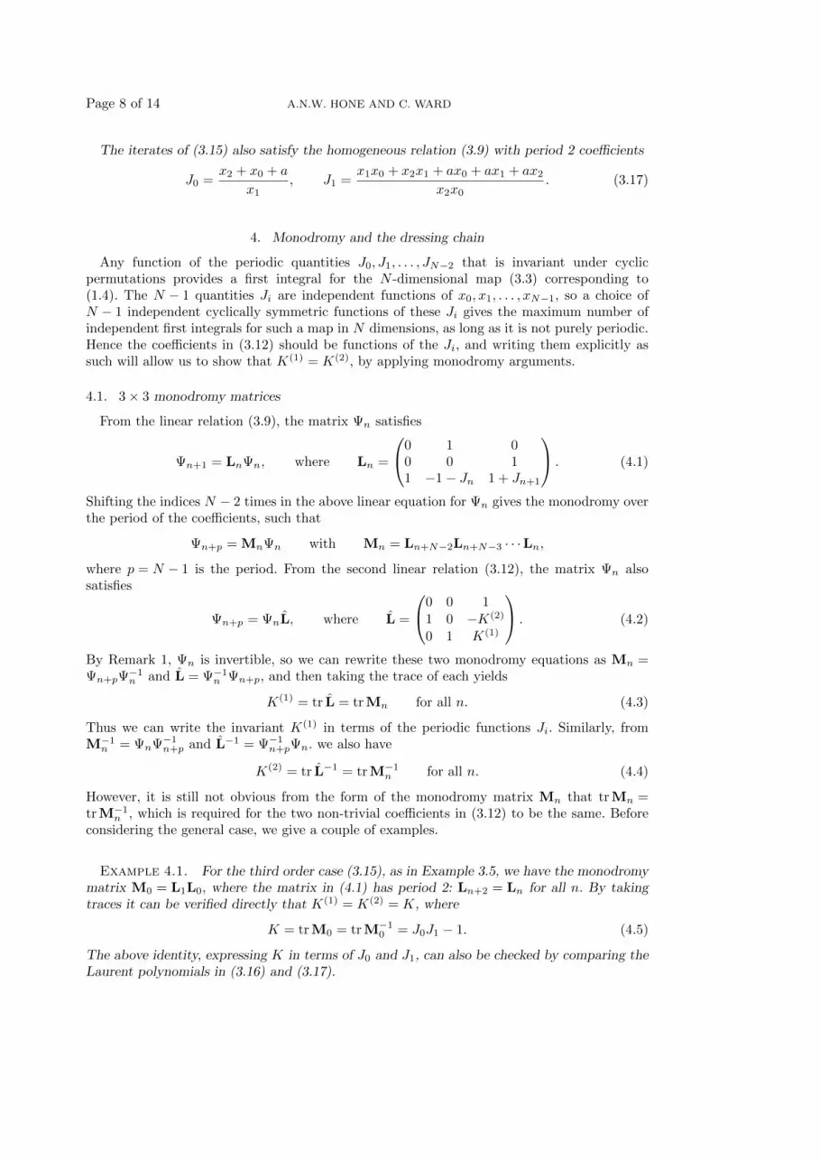
The iterates of (3.15) also satisfy the homogeneous relation (3.9) with period 2 coefficients

J0 =x2 + x0 + a

x1, J1 =

x1x0 + x2x1 + ax0 + ax1 + ax2x2x0

. (3.17)

4. Monodromy and the dressing chain

Any function of the periodic quantities J0, J1, . . . , JN−2 that is invariant under cyclicpermutations provides a first integral for the N -dimensional map (3.3) corresponding to(1.4). The N − 1 quantities Ji are independent functions of x0, x1, . . . , xN−1, so a choice ofN − 1 independent cyclically symmetric functions of these Ji gives the maximum number ofindependent first integrals for such a map in N dimensions, as long as it is not purely periodic.Hence the coefficients in (3.12) should be functions of the Ji, and writing them explicitly assuch will allow us to show that K(1) = K(2), by applying monodromy arguments.

4.1. 3× 3 monodromy matrices

From the linear relation (3.9), the matrix Ψn satisfies

Ψn+1 = LnΨn, where Ln =

0 1 00 0 11 −1− Jn 1 + Jn+1

. (4.1)

Shifting the indices N − 2 times in the above linear equation for Ψn gives the monodromy overthe period of the coefficients, such that

Ψn+p = MnΨn with Mn = Ln+N−2Ln+N−3 · · ·Ln,

where p = N − 1 is the period. From the second linear relation (3.12), the matrix Ψn alsosatisfies

Ψn+p = ΨnL, where L =

0 0 11 0 −K(2)

0 1 K(1)

. (4.2)

By Remark 1, Ψn is invertible, so we can rewrite these two monodromy equations as Mn =Ψn+pΨ−1n and L = Ψ−1n Ψn+p, and then taking the trace of each yields

K(1) = tr L = trMn for all n. (4.3)

Thus we can write the invariant K(1) in terms of the periodic functions Ji. Similarly, fromM−1n = ΨnΨ−1n+p and L−1 = Ψ−1n+pΨn. we also have

K(2) = tr L−1 = trM−1n for all n. (4.4)

However, it is still not obvious from the form of the monodromy matrix Mn that trMn =trM−1n , which is required for the two non-trivial coefficients in (3.12) to be the same. Beforeconsidering the general case, we give a couple of examples.

Example 4.1. For the third order case (3.15), as in Example 3.5, we have the monodromymatrix M0 = L1L0, where the matrix in (4.1) has period 2: Ln+2 = Ln for all n. By takingtraces it can be verified directly that K(1) = K(2) = K, where

K = trM0 = trM−10 = J0J1 − 1. (4.5)

The above identity, expressing K in terms of J0 and J1, can also be checked by comparing theLaurent polynomials in (3.16) and (3.17).


Example 4.2. For N = 4 the nonlinear recurrence (1.4) becomes

xn+4xn = xn+3xn+1 + a(xn+1 + xn+2 + xn+3).

The functions defined by (3.7), which appear as entries in (4.1), have period 3. They are

J0 =x0 + x2 + a

x1, J1 =

x1 + x3 + a

x2, J2 =

x0x2 + x1x3 + a(x0 + x1 + x2 + x3)

x0x3,

with Jn+3 = Jn for all n. Upon taking the trace of monodromy matrix M0 = L2L1L0, andthat of its inverse, it follows from (4.3) and (4.4) that K(1) = K(2) = K, where

K = J0J1J2 − (J0 + J1 + J2) + 1 (4.6)

is the explicit formula for K as a symmetric function of J0, J1, J2.

4.2. Connection with the dressing chain

A one-dimensional Schrodinger operator can be factorised as L = −(∂ + f)(∂ − f), where∂ denotes the operator of differentiation with respect to the independent variable, z say, andf = f(z). The dressing chain, as described in [20], is the set of ordinary differential equations

(fi + fi+1)′ = f2i − f2i+1 + αi, (4.7)

where αi are constant parameters, and the prime denotes the z derivative. These equationsarise from successive Darboux transformations Li → Li+1 that are used to generate a sequenceof Schrodinger operators (Li); the nature of the Darboux transformation is such that eachoperator is obtained from the previous one by a reordering of factors and a constant shift:

Li = −(∂ + fi)(∂ − fi) −→ Li+1 = −(∂ − fi)(∂ + fi) + αi = −(∂ + fi+1)(∂ − fi+1).

Of particular interest is the periodic case, where Li+p = Li for all i. In that case, all indicesin (4.7) should be read mod p, and this becomes a finite-dimensional system for the fi. Asnoted in [20], the properties of this system depend sensitively on the parameters αi: when∑

i αi 6= 0 the general solutions correspond to Painleve transcendents or their higher orderanalogues (see [19] and references for further details), while for

∑i αi = 0 the solutions are of

an algebro-geometric nature, corresponding to finite gap solutions of the KdV equation; thelatter connection goes back to results of Weiss [21].

Here we are concerned with the case∑

i αi = 0 only, so following [20] we use parametersβi such that αi = βi − βi+1 mod p. For p odd there is an invertible transformation fi to newcoordinates, that is

Ji = fi + fi+1, i = 1, . . . , p, (4.8)

and in [20] (where the coordinates Ji are denoted gi) it was shown that in this case theperiodic dressing chain is a bi-Hamiltonian integrable system, meaning that it has a pencilof compatible Poisson brackets together with the appropriate number of Poisson-commutingfirst integrals to satisfy the requirements of Liouville’s theorem. (For p odd the transformation(4.8) is not invertible, but there is a degenerate Poisson bracket for the dressing chain suchthat it is an integrable system on a generic symplectic leaf.) A recent development was theobservation in [9] that (with all βi = 0) a combination of these compatible brackets for thedressing chain coordinates Ji arises by reduction from the log-canonical Poisson structure forthe cluster variables in cluster algebras associated with affine A-type Dynkin quivers. In thiscontext, a further observation was that the linear relations between cluster variables found in[7] (see also [2, 8, 16]), which are of the form

xn+2p − κxn+p + xn = 0, (4.9)


have a non-trivial coefficient κ which is the generating function for the first integrals of thedressing chain (expressed in terms of suitable variables Ji). The key to understanding theseobservations is the following result, which is omitted from the published version of [9] butappeared in the original preprint.

Lemma 4.3. If a 2× 2 monodromy matrix is defined by

M∗ =

(0 ζ11 J1

) (0 ζ21 J2

). . .

(0 ζp1 Jp

), (4.10)

then (with indices read mod p) the trace is given by the explicit formula

trM∗ =

p∏i=1

(1 + ζi

∂2

∂Ji∂Ji+1

) p∏n=1

Jn.

Proof. This is very similar to the proof of Theorem 2 in [20], where a Lax equation for thedressing chain is given for a different monodromy matrix, written in terms of the variables fi.The above identity for the trace of M∗ follows by calculating the coefficient of each monomialin the ζj on either side of the equation, using the relations(

0 01 J1

) (0 01 J2

). . .

(0 01 J`

)= J1J2 . . . J`−1

(0 01 J`

)and (

0 01 Jj

) (0 10 0

) (0 01 Jk

)=

(0 01 Jk

),

and noting that in the latter relation the central matrix on the left is nilpotent.

Remark 2. For the period p dressing chain (4.7) with αi = βi − βi+1, the Poisson-commuting first integrals are found in terms of the variables Ji by setting ζi = βi − λ in (4.10)and expanding trM∗ in powers of the spectral parameter λ.

The 2× 2 monodromy matrix (4.10) also provides the key to understanding the detailedstructure of the linear relation (3.8) associated with (1.4).

Theorem 4.4. In terms of the quantities Jn defined in (3.7), the coefficient K in (3.8) isgiven by the formula

K = 1 +

p∏i=1

(1− ∂2

∂Ji∂Ji+1

) p∏n=1

Jn. (4.11)

Proof. Upon introducing the 2× 2 matrices

Φn =

(xn xn+1

xn+p xn+p+1

), L∗n =

(0 −11 J1

), C =

(0 10 1

),

the inhomogeneous linear equation (3.14) implies that

Φn+1 = ΦnL∗n − aC. (4.12)

Seeking an appropriate inhomogeneous counterpart of (3.8), we define the matrix

M∗n = L∗nL∗n+1 · · ·L∗n+p−1,


which (up to cyclic permutations) is a special case of the monodromy matrix M∗ above,obtained from (4.10) by setting ζi = −1 for all i. Now, by applying a shift to (4.12), we have

Φn+2 = (ΦnL∗n − aC)L∗n+1 − aC = ΦnL

∗nL∗n+1 − aC(L∗n+1 + I)

(with I being the 2× 2 identity matrix), and so by induction, after a total of p− 1 shifts, wefind that

Φn+p = ΦnM∗n − aCKn, (4.13)

where

Kn = L∗n+1 · · ·L∗n+p−1 + L∗n+2 · · ·L∗n+p−1 + . . .+ L∗n+p−1 + I.

Note that the entries of L∗n, and hence those of M∗n and Kn, are all periodic with period p,so from (4.13) it follows that

Φn+2p = Φn+pM∗n − aCKn = Φn(M∗n)2 − aCKn(M∗n + I).

The latter equation can be further simplified with the use of the Cayley-Hamilton theorem,which gives

(M∗n)2 − κM∗n + I = 0, with κ = trM∗n,

and hence (after using (4.13) once again) we find

Φn+2p = κΦn+p − Φn − aCKn

(M∗n + (1− κ)I

).

The (1, 1) entry of the above matrix equation yields an inhomogeneous version of (4.9), namely

xn+2p − κxn+p + xn + aJn = 0, (4.14)

where the quantity Jn is periodic with period p. We claim that this is the desired inhomogeneouscounterpart of (3.8). Indeed, applying the shift n→ n+ p to (4.14) and then subtracting theoriginal equation gives

xn+3p − (κ+ 1)(xn+2p − xn+p

)− xn = 0,

which is (3.8) with K = κ+ 1, and the formula (4.11) then follows from Lemma 4.3. This alsoverifies that K(1) = K(2) in (3.12), completing the missing step in the proof of Theorem 3.3.

Remark 3. Observe that 1 is a root of the characteristic polynomial of the linear relation(3.8), which means that this homogeneous equation is a total difference. Hence, using S todenote the shift operator, we obtain the relation(

S3p−1 + . . .+ S2p − κ(S2p−1 + . . .+ Sp) + Sp−1 + . . .+ S + 1)xn + aK = 0,

where K is a first integral. In the case p = N − 1 = 2, a formula for K as a Laurent polynomialin the initial data can be found in [14] (see Theorem 5.1 therein). Although we do not havea general formula for K, analogous to (4.11), direct calculation shows that K = J0 + J1 + 4for p = 2, and K = J0J1 + J1J2 + J2J0 + 2(J0 + J1 + J2) + 3 for p = 3. Moreover, in the casesp = 2, 3, 4, 5 we have verified with computer algebra that K is given in terms of the 3× 3determinant (3.4) by

K =µ

a3,

and we conjecture that this is always so.

Remark 4. The form of the inhomogeneous relation (4.14) means that the solution of theinitial value problem for (1.4) can be written explicitly using Chebyshev polynomials of the


first and second kind with argument κ/2, that is

Tj(cos θ) = cos jθ, Uj(cos θ) =sin(j + 1)θ

sin θ, where κ = 2 cos θ.

For details of the solution in the case N = 3, see Proposition 5.2 in [14].

5. Conclusions

We have shown that each of the nonlinear recurrences (1.4) fits into the framework of Lamand Pylyavskyy’s LP algebras, implying that the Laurent property holds. Furthermore, eachrecurrence is linearisable in two different ways: with a constant-coefficient homogeneous linearrelation, and with another such relation with periodic coefficients. The connection betweenthe first integral K in (3.8) and the Poisson-commuting first integrals of the dressing chain isintriguing: it raises the question of whether LP algebras might admit natural Poisson and/orpresymplectic structures, analogous to those for cluster algebras [11].

The recurrences (1.5) considered by Heideman and Hogan also possess the Laurent property.(See [13] for a more detailed discussion.) It can also be shown that, beyond the linear relation(1.6) for a particular integer sequence, the result of Proposition 1.1 extends to arbitrary initialdata. In this case there is also an analogue of (3.9), with periodic coefficients, but with a morecomplicated structure. These results will be presented elsewhere.

To conclude we should like to mention that, after this paper was submitted, Pavlo Pylyavskyymade us aware of recent work by Alman, Cuenca and Huang, who independently found therecurrences (1.4) within the context of LP algebras: see family (3) in Theorem 3.9 of thepreprint [1].

6. Appendix

Here we consider the particular family of integer sequences that is generated by iteratingeach recurrence (1.4) with all N initial data set to the value 1, and prove the following result.

Theorem 6.1. For each N ≥ 2, the recurrence (1.4) with initial values xn = 1 for n =0, . . . , p = N − 1 generates a sequence of integers (xn) which is symmetric in the sense thatxn = xp−n for all n ∈ Z. The first few terms are given by

xp+j = f2j p+ 1, x2p+j = f2jf2p p2 +

(f2j(f2p+2 + 1)− f2j−2f2p

)p+ 1, j = 0, . . . , p. (6.1)

In general, for each k ≥ 0 the terms xkp+j for 1 ≤ j ≤ p can be written as polynomials in pwhose coefficients are themselves polynomials in Fibonacci numbers with even index.

First of all, to see why xn = xp−n, observe that the nonlinear recurrence (1.4) has two obvioussymmetries: translating n, and replacing n by −n. Combining these two symmetries, it followsthat the sequence (xp−n) satisfies (1.4) whenever the sequence (xn) does; the fact that theinitial data 1, 1, . . . , 1 is symmetric under n→ p− n implies that these two sequences coincide.

The rest of the proof proceeds inductively, and relies on various identities for Fibonaccinumbers; note that the convention f0 = 0, f1 = 1 is taken for the initial Fibonacci numbers.From the Fibonacci recurrence fn+2 = fn+1 + fn it follows that the even index terms satisfy

f2n+4 = 3f2n+2 − f2n. (6.2)


For n = 0, . . . , p− 1 the relation (1.4) is satisfied by the initial data and the first set of termsin (6.1) by virtue of the identity

f2n+2 − f2n = f2n + f2n−2 + . . .+ f2 + 1, (6.3)

which follows from (6.2) by induction. To verify the formula for the second set of terms in(6.1), it suffices to substitute these expressions into (1.4) with n = p, . . . , 2p− 1 and comparecoefficients of powers of p on both sides, making use of (6.3) again, together with the identity∣∣∣∣ f2j−2 f2j

f2j f2j+2

∣∣∣∣ = −1.

The fact that the latter 2× 2 determinant is a constant (independent of j) follows from (6.2),while the value −1 is obtained immediately from f0 = 0, f±2 = ±1.

Proposition 1.2 is now seen to be a special case of Theorem 3.3, by making use of Theorem 6.1.Indeed, from (3.8) with n = j − p for 1 ≤ j ≤ p, the above choice of initial data and the termsin (6.1), as well as the symmetry of the sequence, yields K = (x2p+j − x−p+j)/(xp+j − xj) =(x2p+j − x2p−j)/(xp+j − xj) = f2pp+ f2p+2 + 1− (f2j−2f2p + f2p−2j)/f2j . In order to see whythe latter expression is a constant (independent of j), and to obtain the particular form ofthe coefficient K that appears in (1.7), it is enough to verify the identity f2jf2p−2 − f2j−2f2p =f2p−2j , which is done by writing the even index Fibonacci numbers as f2n = sinhnθ/sinh θ with

θ = log(

3+√5

2

), and using the addition formula for the hyperbolic sine.

References

1. J. Alman, C. Cuenca and J. Huang, Laurent Phenomenon Sequences, (2013), arXiv:1309.0751v22. I. Assem, C. Reutenauer and D. Smith, Friezes, Adv. Math. 225, (2010) 3134-3165.3. P. Di Francesco, Discrete integrable systems, positivity and continued fraction rearrangements, Lett.

Math. Phys. 96 (2011) 299-324.4. C.L. Dodgson, Condensation of determinants, Proc. R. Soc. Lond., 15, (1866) 150-155.5. S. Fomin and A. Zelevinsky, Cluster algebras I: Foundations, J. Amer. Math. Soc. 15 (2002) 497-529.6. S. Fomin and A. Zelevinsky, The Laurent Phenomenon, Advances in Applied Mathematics 28 (2002)

119-144.7. A.P. Fordy and R.J. Marsh, Cluster Mutation-Periodic Quivers and Associated Laurent Sequences, J.

Algebr. Comb., 34 (2009) 19-66.8. A.P. Fordy, Mutation-Periodic Quivers, Integrable Maps and Associated Poisson Algebras, Philos. Trans.

R. Soc. Lond. Ser. A, 369 (2010) 1264-1279.9. A.P. Fordy and A.N.W. Hone, Discrete integrable systems and Poisson algebras from cluster maps,

Commun. Math. Phys. (2013) at press, arXiv:1207.6072v210. D. Gale, The strange and surprising saga of the Somos sequences, Mathematical Intelligencer 13 (1) (1991)

40–42.11. M. Gekhtman, M.Shapiro and A. Vainshtein, Cluster algebras and Weil–Petersson forms, Duke Math. J.

127 (2005), 291–311.12. P. Heideman and E. Hogan, A New Family of Somos-like Recurrences, Elec. J. Comb., 15, (2008) #R54.13. E. Hogan, Experimental Mathematics Applied to the Study of Nonlinear Recurrences, PhD thesis, Rutgers

University, 2011.14. A.N.W. Hone, Nonlinear recurrence sequences and Laurent polynomials, Number Theory and Polynomials

(ed. J.McKee and C. Smyth), LMS Lecture Note Series, 352, (2008) 188-210.15. R. Kedem, Q-Systems as cluster algebras, J. Phys. A. 41 (2008) 194011.16. B. Keller and S. Scherotzke, Linear recurrence relations for cluster variables of affine quivers, Adv.

Math. 228, (2011) 1842-186217. T. Lam and P. Pylyavskyy, Laurent phenomenon algebras, (2012), arXiv:1206.2611v218. W. Nahm and S. Keegan, Integrable deformations of CFTs and the discrete Hirota equations,

arXiv:0905.3776v219. K. Takasaki, Spectral Curve, Darboux Coordinates and Hamiltonian Structure of Periodic Dressing

Chains, Commun. Math. Phys. 241 (2003) 111–142.20. A.P. Veselov and A.B. Shabat, Dressing chains and the spectral theory of the Schrodinger Operator,

Funct. Anal. Appl., 27, (1993) 81–96.21. J. Weiss, Periodic fixed points of Backlund transformations and the KdV equation, J. Math. Phys., 27

(1986) 2647–2656.


A.N.W. Hone and C. WardSchool of Mathematics, Statistics &

Actuarial ScienceUniversity of Kent, Canterbury CT2 7NFU.K.

[email protected]@kent.ac.uk

Documents

A family of linearizable recurrences with the Laurent property