PROPERTY TAXES AND PROPERTY VALUES:EVIDENCE FROM PROPOSITION 2½

Kevin Lang Department of Economics

Boston University270 Bay State RoadBoston MA 02215

and

Tianlun JianMassachusetts Financial Services

Boston, MA

Latest Revision: August 3, 2000

This research was supported in part by NSF grant SBR-9515052. We are grateful to Eli Berman, HarveyBeth, Kathy Bradbury, John Conley, Dennis Epple, Ed Glaeser, Hideo Konishi, Jim Poterba, Brian Sullivanand participants in the Boston University Applied Microeconomics workshop and the 1997 ASSAmeetings for helpful comments and discussions. We thank Roger Hatch, John Sanguinet, and Julie Slavetof the Massachusetts Department of Revenue and Donald Buckhotz and Scott Keese of the MassachusettsTaxpayers Foundation for providing data and other assistance. The usual caveat applies.

ABSTRACT

We examine the effect of Proposition 2½ on revenues and housing prices in Massachusetts.Communities that were initially constrained by the law, saw large increases in state aid and the use offees. We use these initial constraints as instruments for changes in other components of revenue whiletreating the change in the property tax as exogenously determined by Proposition 2½ . Our resultsstrongly suggest that communities that were able to increase their property taxes more rapidly sawgreater increases in their housing values in the period following passage of the law.

1The rules governing tax increases for bond issues are somewhat different. We skip over thesedetails since they are unimportant for the purposes of this paper.

I. Introduction

In November 1980, Massachusetts voters passed a tax revolt law commonly known as

Proposition 2½. Subject to certain exceptions, the law limited the property tax rate to 2½% of the

assessed value of property. Communities with tax rates in excess of 2½% were required to reduce their

tax revenues by 15% per year until they complied with the law. Almost half of Massachusetts

communities had to cut taxes in the first year the law was in effect. Two communities required four years

to reach compliance with the tax rate limitation. Once the tax rate limit has been met, Proposition 2½

invokes a tax levy limit. Communities can set taxes below the levy limit but may not exceed it. The levy

limit on existing property increases by 2½% (nominal) per year. However, if a community chooses not

to tax at its limit one year, it does not affect the levy limit. Thus if a community that is taxing at its limit

chooses not to increase its taxes one year so that it is approximately 2½% below its limit, the following

year it may increase taxes by approximately 5%. New growth in a given year can be added to the tax

base and taxed at the community's normal tax rate. Thereafter, it becomes part of the tax base and is

subject to the 2½% growth limitation.

Communities may also increase their levy limit by submitting a Proposition 2½ override to the

electorate.1 By the end of the period we study, the levy limit rather than the tax rate limit was the

constraining factor for those communities constrained by the law. In principle, therefore, communities

were not constrained since they had the option to vote further tax increases. In practice, during the

period we study, relatively few communities passed overrides while many were at or near their levy

limits. This suggests that by requiring an override, the levy limit did constrain taxes.

2

2For a review of the Massachusetts economy and state economic policy from 1975 to 1986 seeFerguson and Ladd, 1986.

Proposition 2½ significantly changed both the level and composition of local government

revenues. Real per capita local government revenues declined from 1981 to 1984 and did not regain

their 1981 level until 1988 despite a booming Massachusetts economy over this period.2 As of 1992,

real per capita local revenues were less than 3% above their pre-Proposition 2½ level. Moreover, real

per capita property taxes declined and remained almost 10% below their pre-Proposition 2½ level in

1992. The loss was made up in part by increased state aid which rose dramatically between 1981 and

1988 and then declined sharply. The rest of the loss was made up by increases in fees and charges

which increased by close to 80% going from 11% to 18% of local government revenues between 1981

and 1992.

It would be unfair to describe Proposition 2½ as a "natural experiment." The law was crafted by

people not nature. Nevertheless, the institutional structures it generated and the changes it imposed on

communities allow us to identify the impact of local government spending and revenue structure on

property values.

The popular debate over tax limitation measures primarily concerns two different conceptions of

government. Supporters maintain that local governments are run by inefficient bureaucracies and believe

that budgets can be cut without a significant reduction in services. Opponents generally believe that

reducing tax revenues will reduce services (Ladd and Wilson, 1982). The two views are not necessarily

in contradiction -- local government could be inefficiently run, but given inherent inefficiencies, services

might be provided at the level desired by the electorate.

In economists' terms, the issue is whether government provides the desired level of public goods

3

given constraints on its behavior. These may include union rent-seeking, difficulties motivating workers,

(political or legal) requirements that they pay above market wages, etc. If part of any tax increase is

captured by government workers, reducing taxes will restrain wages but will also lower utility if

government has already taken the impact of tax revenues on wages into account when setting tax levels.

In order to examine the maximization hypothesis, we develop a model in which utility differences

are capitalized into housing prices. There is a tendency in the literature for papers concerned with the

effects of interjurisdictional variation in taxes or services (e.g. Polinsky and Rubinfeld, 1978; Case and

Grant, 1991) to work within a framework derived from the Tiebout model. However, other models will

have similar features. Hobson (1986) shows that when the population is fully mobile, differences in tax

rates across communities (holding services constant) will be capitalized into land rents. Thus while the

burden of the average property tax rate may be shifted among factors of production or to renters

depending on supply and substitution elasticities, land rents capture property tax differentials. The link

between service levels and taxes on the one hand and property values on the other is quite general

(Mieszkowski/Zodrow, 1989).

Oates's path-breaking paper (1969) was the first to confront the inter-jurisdictional capitalization

hypothesis empirically. He argued that the Tiebout model implies that services will increase property

values while taxes will reduce them and confirmed these predictions. However, Edel and Sclar (1974),

Hamilton (1976) and Meadows (1976) pointed out that in Tiebout equilibrium land values are

independent of the level of service provided. Therefore, either the New Jersey municipalities were not in

equilibrium or the Tiebout model requires modification. The ensuing research has tended to present itself

as either examining disequilibrium or studying whether service and tax differentials are capitalized into

housing values without directly relating the research to the Tiebout model (see Shenkel and Gaines,

4

1978; Brueckner, 1979; Taylor, 1991; and related work by Ladd and Bradbury, 1988).

Testing for capitalization within a Tiebout model is problematic, because the model suggests no

obvious reason why public services and tax levels should not be perfectly related. Under the Tiebout

model, either service levels or tax levels is a sufficient statistic for public good provision (Hamilton,

1976). Conditional on the service level, the tax rate is therefore purely a measure of house values.

Since housing values are in the denominator of the tax rate, the tax rate variable will be negatively

correlated with housing values. Since tax levels and service levels are positively correlated, OLS

estimates will tend to generate a positive coefficient on service levels and a negative coefficient on tax

rates even if we are in full Tiebout equilibrium.

Oates recognized the difficulties with the endogeneity of taxes and services and proposed a

2SLS estimator. However, Pollakowski (1973) challenged the choice of instruments. We can translate

his argument into somewhat more modern language. There is a hedonic relation between housing prices

and housing characteristics including the local public finance characteristics. If we need to instrument for

local taxes and services, we must find variables that influence their levels but are not correlated with the

error term. Since the error term includes any unmeasured housing characteristics, it is difficult to think of

factors that affect the demand for local public goods but for which we can convincingly argue that they

do not affect the demand for other housing characteristics. In the absence of the Tiebout model, we face

the opposite problem. Without a well-formulated theory of why spending and service levels differ, it is

difficult to argue convincingly whether instruments are needed or what are potential instruments.

The approach taken here is somewhat different. We use the experiment induced by Proposition

5

3Bradbury, Mayer and Case (1996) also uses Proposition 2½ to generate instruments for fiscalvariables. The relation between our results and the results in that paper is discussed in the conclusion.

2½ to avoid the problem of the lack of suitable instruments.3 We treat Proposition 2½ as a constraint

on government optimization. More heavily constrained communities will be further from the optimum

and hence will suffer larger declines in housing prices.

II. The Model

The model developed in this section is oriented towards laying the ground work for our empirical

analysis. It therefore does not include much of the richness of recent research on Tiebout economies

(see Conley and Wooders, 1997, for a review). In particular, since we consider the effects of

Proposition 2½ over a short period, we treat both the aggregate housing stock and its distribution across

communities as fixed. We also ignore consumer heterogeneity and concentrate on the consequences of

heterogeneity across communities.

Each community provides a public good which we think of as education since most

Massachusetts communities spend over half their budget on education. Public education must be

provided to all members of the community on an equal basis. However, the cost of providing education

of a given quality is a fixed amount per member of the population. Thus the public good is really a

publicly provided private good or in Bewley’s (1981) terminology, a pure public service. Since the size

of each community is fixed, the community cares only about the average (or total) cost of providing

education to its residents. We thus ignore aggregate crowding issues.

A1. The cost of producing the public good in community i is ciG per member of the community

where ci is the marginal cost of producing the good and G is the number of units of the public

good provided to each member of the community.

6

G can be thought of as school quality. It should be noted that the marginal cost of a unit of quality varies

across communities. This assumption is the major departure from the standard model which typically

assumes that all communities face the same cost structure. “c” may capture the reputation of the local

school system. If the schools already have a good reputation, it may be cheaper to produce good

schools than if they start off with a poor or indifferent reputation. In a more complex model this might

capture peer effects. Costs might also differ because of varying ability of public sector unions to capture

rents along the lines discussed in Gyourko and Tracy (1989, 1991) or the presence of an exogenous

amenity that is complementary with the public good. Note that the communities differ with regard to the

marginal cost of producing G. Differences in fixed costs will be capitalized into housing prices but will

not alter the level of the good provided. Provided that all types want at least some of the public good,

fixed costs do not affect the allocation of types to communities.

We find it natural to assume that marginal cost varies among communities once we recognize that

history matters. In a fuller model with heterogeneous consumers, the cost of providing the good might

depend on the characteristics of the population (Conley and Wooders, 1997). We believe that our

estimating equation would be justified in such a model, but the technical difficulties of developing the

theory would be much greater.

Alternatively, the public good could be a combination of, for example, schooling and clean air

with the level of air quality outside the control of the community. Even if the cost of providing a given

level of school quality is the same in all communities, the cost of providing the composite public good will

be higher in areas with bad air quality.

A2. The public good may be financed through property taxes, T, state aid, A, and/or fees, F.

Property taxes are subsidized at rate t through the income tax system while fees are not so that

7

the net cost to residents is (1-t)T+F. The rental cost of housing is h+(1-t)T+F.

It is evident that fees are dominated by property taxes in the absence of constraints on property

taxation. Fees will only be used in the presence of a measure limiting the tax rate and therefore will be

ignored for the moment.

A3. There are a homogeneous private good that serves as numeraire and a homogeneous public

good (G). There is a large number of homogeneous individuals with differentiable utility u(Y-p,G)

where Y is exogenous income and p is the rental cost of housing including taxes. u is assumed to

be quasi-concave and twice differentiable with (Mu/MY)Y-p=0=(Mu/MG)G=0 = 4.

It should be noted that Y is assumed to be independent of the level of the public good.

Massachusetts communities are small relative to the labor market in which they operate. We therefore

do not believe that the provision of public goods to residents in any one community could affect wages

either in that community relative to other communities or in the labor market as a whole. In principle,

providing public goods to workers in a community could affect wages, but the goods provided by

Massachusetts communities are overwhelmingly oriented towards residents. In particular, spending on

education typically accounts for half or more of all local spending.

A4. The housing stock is fixed and homogeneous.

Thus, we abstract from the effects of property taxation on the quality of housing. Since we will

be examining interjurisdictional effects within Massachusetts, it seems safe to ignore the impact of the law

on the return to capital in the United States. On the other hand, it is possible that Proposition 2½

affected the nature of housing in the state. Our empirical work covers the period from 1984 to 1988.

The stock of housing was large relative to new construction over this period. If anything the reduction in

taxes should have increased new construction. We therefore believe that we will not violate reality

8

significantly if we treat the housing stock as fixed.

A5. Each community chooses the level of the public good to maximize the utility of a

representative resident.

We define an equilibrium as one with T, F, h and G related to c so that no individual wishes to

move:

(1) u(Y-(1-t)T(c)-F(c)-h(c), G(c)) = u*

for all inhabited communities and

(2) u(Y-(1-t)T(c)-F(c), G(c)) < u*

for all uninhabited communities. All communities with cost below some critical value of c will be

inhabited while the remaining communities will not. No individual will want to move if housing prices, G,

T and F are set such that individuals are indifferent among all communities with a positive population and

utility is below this level for unpopulated communities even when the price of housing is 0.

Given that individuals are homogeneous, the equilibrium entails each community choosing G such

that

(3) (1-t)cu1=u2,

and setting T=cG and F=0. h then adjusts to ensure that conditions (1) and (2) hold.

Although the level of the public good and housing prices are positively correlated, the correlation

between the tax rate and housing prices or the tax level and housing prices may be positive or negative.

To see this, note that if the elasticity of demand for public goods is greater than -1, total expenditure on

public goods (taxes) will be higher in communities where their marginal cost is higher. These are also the

communities in which housing prices are lowest. So the tax level and housing prices will be negatively

correlated. If the elasticity is less than -1, the tax level and housing prices will be positively correlated.

9

If the demand for public goods is sufficiently elastic, the tax rate and housing prices will be positively

correlated. This suggests that attempts to test Tiebout-type models on cross-section data are not likely

to be informative.

The assumption that individuals are homogeneous is clearly strong, but it largely serves to

eliminate technical difficulties. Under a condition such as that used by Westhoff (1977) to ensure sorting

of types in equilibrium, equation (1) will hold for marginal individuals. If communities are sufficiently

homogeneous, the choice of the public good in each community will satisfy (3) approximately for each

resident.

We eliminate G to get the utility of a representative resident as a function of housing prices and

revenue variables alone

(4) u = u(Y - h - (1-t)T - F, [A+T+F]/c).

Under Proposition 2½ communities are constrained to keep their tax rate below .025 so that

T<.025h. If this constraint is binding, we have

(5) u2c > u1 > u2(1-t)c, T = bh

with the first inequality being strict only if F>0.

It is not clear to what extent communities in Massachusetts are actually free to set fees optimally.

State law prevents fees from exceeding the cost of providing the service. There is some flexibility in

defining the service (e.g. recreation versus golf, tennis, basketball, etc.) and some ability to inflate the

cost of services by decisions regarding the allocation of fixed costs. Still, we are aware that at least

some communities viewed themselves as constrained by the limit on fees.

Both in the presence and absence of constraints on taxes, housing prices adjust so that

individuals are just indifferent between living in their own community and one with almost the same cost

10

4In a more general model individuals and communities would be matched on the basis of tastes andcosts. In this case, we would need to assume that the law did not change which communities andindividuals were matched. There are situations in which this assumption would not be reasonable. Forexample if laws limiting taxes applied only to some communities, a community with a low cost ofproducing the public good might be constrained to produce less of the public good than a higher costcommunity. In this case, it is likely that the individuals with a stronger desire for the public good wouldend up in the higher cost community. Given the universal nature of Proposition 2½ withinMassachusetts, this does not appear to be a concern in our case.

of producing the public good:

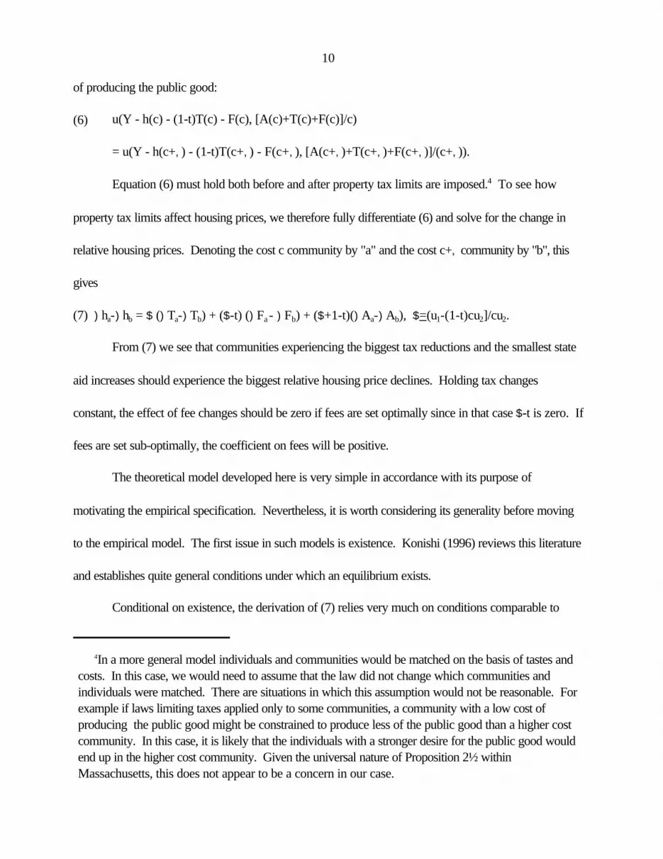
(6) u(Y - h(c) - (1-t)T(c) - F(c), [A(c)+T(c)+F(c)]/c)

= u(Y - h(c+,) - (1-t)T(c+,) - F(c+,), [A(c+,)+T(c+,)+F(c+,)]/(c+,)).

Equation (6) must hold both before and after property tax limits are imposed.4 To see how

property tax limits affect housing prices, we therefore fully differentiate (6) and solve for the change in

relative housing prices. Denoting the cost c community by "a" and the cost c+, community by "b", this

gives

(7) )ha-)hb = $ ()Ta-)Tb) + ($-t) ()Fa - )Fb) + ($+1-t)()Aa-)Ab), $=(u1-(1-t)cu2]/cu2.

From (7) we see that communities experiencing the biggest tax reductions and the smallest state

aid increases should experience the biggest relative housing price declines. Holding tax changes

constant, the effect of fee changes should be zero if fees are set optimally since in that case $-t is zero. If

fees are set sub-optimally, the coefficient on fees will be positive.

The theoretical model developed here is very simple in accordance with its purpose of

motivating the empirical specification. Nevertheless, it is worth considering its generality before moving

to the empirical model. The first issue in such models is existence. Konishi (1996) reviews this literature

and establishes quite general conditions under which an equilibrium exists.

Conditional on existence, the derivation of (7) relies very much on conditions comparable to

11

5In Epple et al (1984), the requirement is that higher income individuals be located in communitieswith higher levels of the public good. A comparable result will occur in this model regarding tastes andthe level of the public good. However, as noted, we make a stronger assumption regarding efficientmatching.

those that Epple at al (1984) argue will be present in any equilibrium -- stratification (segmentation of

communities by type), boundary indifference (the border consumer is indifferent between two

communities), and ascending bundles (in this case the relation between costs and tastes).5 Complete

stratification is not necessary. Epple et al (1978) show that a model in which communities are sorted

by type of individual but are too large to be perfectly homogeneous and in which the level of public good

provision is determined by the median voter generates results that are quite close to the Tiebout model.

The work of Nechyba (1997) is perhaps the most directly applicable to this model. He shows

that if the number of communities is finite, for a given type of house, individuals will be stratified by their

preference for the public good. If housing is homogeneous, this result is similar to that of Epple et al

(1978) although it is derived under quite different assumptions. However, if housing is heterogeneous,

some individuals may prefer the public good/tax rate combination of another community. In this case, it

is not obvious that we can make strong statements about the coefficients in (7). Instead the empirical

counterpart of (7) simply becomes an ad hoc estimating equation.

Since neither Nechyba nor the earlier authors allow for communities with differing production

functions, their results are not directly applicable to the empirical work developed here. Nevertheless,

on the basis of those papers, it is reasonable to conclude that adding individual heterogeneity would be

technically difficult but unlikely to change the results. Adding housing heterogeneity would mean that tax

restrictions might affect the prices of different types of houses in different ways.

An additional key feature of the equilibrium is that the allocation of individuals to communities is

12

independent of the tax restriction. This is plausible when the housing stock is exogenous, a common

assumption in models establishing the existence of equilibrium (e.g. Nechyba, 1997). However, when

the housing stock is endogenous, in the absence of strict zoning laws, changes in property taxes may

alter the equilibrium level of congestion and thus which individuals locate in which communities. We rely

on a combination of zoning regulations, and the fact that the housing stock is large relative to new

building to justify our assumption.

Equation (7) models the effects of property tax constraints as working only through their impact

on revenues and not through the level of the public good. Under the assumption that the public good is

homogeneous, total revenue is a sufficient statistic for the level of public good. In reality, of course,

public goods are not homogeneous. Equation (7) therefore requires either that the composition of the

public goods is chosen optimally or that it is independent of the level of revenue.

Finally, although we have modeled fees as independent of use of the public good, this is not

always the case. Some depend on usage as in the case where there is a daily fee for use of the local

swimming pool. Others, provide access to a public good but do not depend on use. Thus, for example,

many Massachusetts communities have a flat annual fee for trash removal. As we would expect from the

model, local receipts (mostly fees and fines) rose significantly following the passage of Proposition 2½.

Our discussions with local officials suggest that the largest growth came from establishing trash fees

which closely approximates the increase in fees modeled above and from very large increases in water

and sewage fees related to the Boston Harbor clean-up, which does not. If demand for services

financed through services is elastic and if the marginal cost of providing the service is positive, fees set

somewhat below marginal cost (to take account of tax advantages) will be efficient.

III. Data and Estimation

13

The approach used here is closest to Rosen (1982) who examines the capitalization of tax rate

reductions following the passage of Proposition 13 in California. Rosen argues that the state bailout left

the change in services nearly uniform across communities while Proposition 13 significantly limited the

ability of communities to find other local sources of funds. For these reasons the approach taken here is

somewhat different.

The data are drawn from the Massachusetts Department of Revenue municipal data bank. The

data bank includes information on tax rates, revenues by source (e.g. property taxes, fees and fines,

state aid). Massachusetts communities are required to reassess all property at 100% of value at least

every three years. Therefore, in principle, all property in Massachusetts is assessed at full market value

at least once every three years. The Massachusetts Department of Revenue releases data on the value

of property in each community every two years. The DOR estimate adjusts the most recent assessment

for developments in the property market since that assessment took place. The data bank also contains

information on the years for which a general reassessment took place so that we can control for

systematic errors in the process by which the DOR adjusts the data from the older assessments.

Unfortunately, although the Classification Law (1979) required all communities to assess property by

class at 100% of market value at least once every three years, some communities did not comply with

the law until 1986.

We choose 1984 as our starting date to balance two concerns -- the need to have precise data

on as many communities as possible and the need to have data sufficiently early to capture the impact of

the constraints imposed by the law. A number of factors suggest that prior to 1984 data problems are

severe. Although the Classification Law was passed in 1979, many communities dragged their feet on

reassessing property. The tax limits imposed by Proposition 2½ created an additional impetus to

14

6Conditional on the community’s reported assessed value, in 1982 the state’s estimates of equalizedvalues were lower for communities that were more heavily constrained by Proposition 2½. This isconsistent with the hypothesis that state estimates were directly influenced by the impact of the law onthe community. It is also, however, consistent with more benign interpretations such as that constrainedcommunities assessed property values more aggressively in order to reduce the Proposition 2½constraint.

revaluation. This process was largely completed by 1984. Prior to 1984 many communities did not

perform full reassessments on a regular basis, giving the state less information on which to base its

estimates of equalized property values. State estimates of the growth of equalized values between 1980

and 1982 are, in fact, highly negatively correlated with the growth between 1982 and 1984 (r=-.32). In

contrast, the correlations between the 1982-84 and 1984-86 and the 1984-86 and 1986-88 growth

rates are approximately 0. This suggests either considerable higher measurement error than usual or a

very significant transitory component to the 1982 levels.

Moreover, the changes in assessed value as reported by municipalities between 1982 and 1984

have little explanatory power for changes in equalized value as estimated by the state over this period. If

we regress the percentage change in equalized value on the percentage change in assessed value and

controls for when the assessments took place, the coefficient on assessed value is .02. Even if we limit

ourselves to communities with reassessments in both 1981-82 and 1983-84, this coefficient rises to only

.51. In contrast, a similar regression for the period 1984-88, restricted to communities with an

assessment in the period 1982-84 (and within three years after the first of these assessments) yields a

coefficient of .99. At the best, this comparison suggests that prior to 1984, the state was working with

very noisy assessment data on which to based its estimate of equalized values. At worst, the state’s

estimate of equalized values may have been directly influenced by the perceived impact of Proposition

2½.6

15

In addition, although the impact of Proposition 2½ was first felt in 1982, there was a great deal

of uncertainty about the law. It is reasonable to expect that individuals understood the workings of the

law and expected it to be upheld by the legislature by 1984.

On the other hand, the law continued to affect municipalities differentially even after 1984.

Cutler, Elmendorf and Zeckhauser (1997, table 4) estimate that a $100 increase in the initial constraint

imposed by Proposition 2½ lowered tax revenues by an additional $13 (from $86 to $99 per $100

initial constraint) between 1984 and 1988 and increased state aid by an additional $50 and total

revenues by an additional $30.

We confirm below that the initial constraints have explanatory power for changes in revenue and

revenue structure for the 1984-88 period. Moreover, as discussed below, changes in revenues between

1982 and 1984 have little in any predictive power for changes between 1984 and 1988, suggesting that

the impact of Proposition 2½ on this period can be studied in isolation.

Our choice to examine changes in property values starting in 1984 implicitly assumes that in

1984 the market did not anticipate the revenue changes that would take place over the next four years.

We find this assumption plausible given the high degree of uncertainty surrounding the impact of the law

and the state of the economy. To cast light on the predictability of the revenue changes, we examined

the correlation of the percentage change in each component of revenue between 1982 and 1984 and the

percentage change between 1984 and 1988. The correlations were .15 for the levy, -.21 for state aid

and -.32 for local receipts. To some extent, these correlations will give a misleading indication of the

predictability of revenue changes if there are random variations in 1984 revenues that are included in the

data but discounted by individuals. As a guard against this problem, we also examined the relations by

regressing the 1984-1988 percentage changes on the 1982-1984 percentage changes using whether or

16

7Preliminary experiments indicated that the results were unaffected by whether we divided by 1980or 1990 population or the earlier period by 1980 and the later period by 1990 population. There wassome tendency for the last approach to lower the coefficient on the tax levy but even this effect wasinconsistent. In none of our experiments did it change the interpretation of the results.

not the community was constrained to lower the levy in 1982 and in 1983 as instruments. The relation

between the earlier and later changes is positive but falls short of significance at the .05 level and the R2 is

less than .025 in all three cases. We therefore conclude that it would have been difficult for individuals in

1984 to fully predict the impact of Proposition 2½ on the level and composition of future revenues. We

therefore find it plausible that the law had effects that were not fully capitalized by 1984. As a further

check on our results, we also experiment with using the change in property values between 1982 and

1984 as the dependent variable with 1984-88 changes in revenue components as explanatory variables.

Our decision to examine changes through 1988 reflects additional concerns. First, initially

Proposition 2½ impacted communities largely by forcing them to reduce their tax rate. By 1986 the tax

rate limit was irrelevant, and the provision limiting tax revenue growth to 2½% became more important.

Finally, the dramatic end of the Massachusetts miracle in 1989 generated renewed disruption, raising

questions about whether markets were fully adjusted to the new environment in the next few years.

Our measure of property values is the Department of Revenue's estimate of the equalized value

of property divided by 1990 population estimates from the U.S. Census.7 This measure has the

advantage of being available for the period prior to Proposition 2½, thereby allowing us to perform

certain checks on our estimation. It is also available for all the observations in our sample. In contrast,

the assessed value of residential housing was not available for 20% of our sample. Moreover,

individuals at the Department of Revenue expressed concern about the accuracy of the assessed value of

residential housing data in 1984. Nevertheless, since we do not have a good measure of nonresidential

17

development, there is a risk that this measure will capture the growth of commercial property rather than

an increase in the value of existing property. Across Massachusetts residential property accounts for

over three-quarters of total assessed value. Nevertheless, if there were significant areas of commercial

development not accompanied by new housing, this could cause a problem for our estimates. We

address this issue below.

By law, assessments must be based on sales of property occurring within a narrow window

around the data of the assessment. As a consequence, communities with few transactions have

inaccurate assessments. These are reflected in large changes in the average assessment. Communities

with fewer than forty property transactions in 1984 are excluded from our restricted sample. This results

in a loss of 76 small communities from the sample all with populations below 6100. We further exclude

from our restricted sample thirteen communities that had not complied with the Classification Law by

1984.

The model applies to communities with a fixed housing stock and to the change in the value of a

fixed stock. The results below exclude communities in which the number of housing units increased by

more than 20% between the 1980 and 1990 censuses. The results in the loss of 84 communities ranging

in population from 1,481 to 49,832 from the restricted sample. The restricted sample contains 178

communities.

Some readers were concerned that our results are driven by our exclusion restrictions. We

therefore present our principal estimates using the full sample of 351 communities. As will be apparent,

these results are better in the sense that they tell a similar story to that of the restricted sample but

present fewer anomalies. Nevertheless, for the reasons outlined above, we prefer the restricted sample

and concentrate on those results.

18

8This implicitly assumes that $ is the same for all communities. Although this assumption is strong, itis not fundamentally different from the standard fixed coefficient assumption for OLS.

Our basic strategy is to estimate an empirical version of equation (7). Before doing so, there are

a number of complications we must address. The major difficulty is that in contrast with the model, the

nature of the housing stock varies among communities. If we assume that, except for the role of revenue

changes, all property would have increased in value at the same rate, we can approximate (7) using a

semi-log equation in which the dependent variable is the change in the log of the equalized value of

property. We regress the dependent variable on the change in real per capita property taxes, real state

aid and real local receipts all measured in 1984 dollars. In addition, because property value increases

may have varied among types of communities, we include six dummy variables for community type as

defined by the Massachusetts Department of Revenue. To guard against systematic errors in adjusting

older assessments, we include dummy variables for the years in which the most recent assessments prior

to 1984 and 1988 took place.

In order to move from equation (7) to an empirical specification, we sum (7) over all

communities and divide by the number of communities to get an expression for

)ha - Eb )hb /N, the difference between the increase in property values in one community versus the

average of all communities as a function of the difference between the change in its revenue components

versus the state average.8 Finally, we note that OLS on levels is equivalent to OLS on deviations from

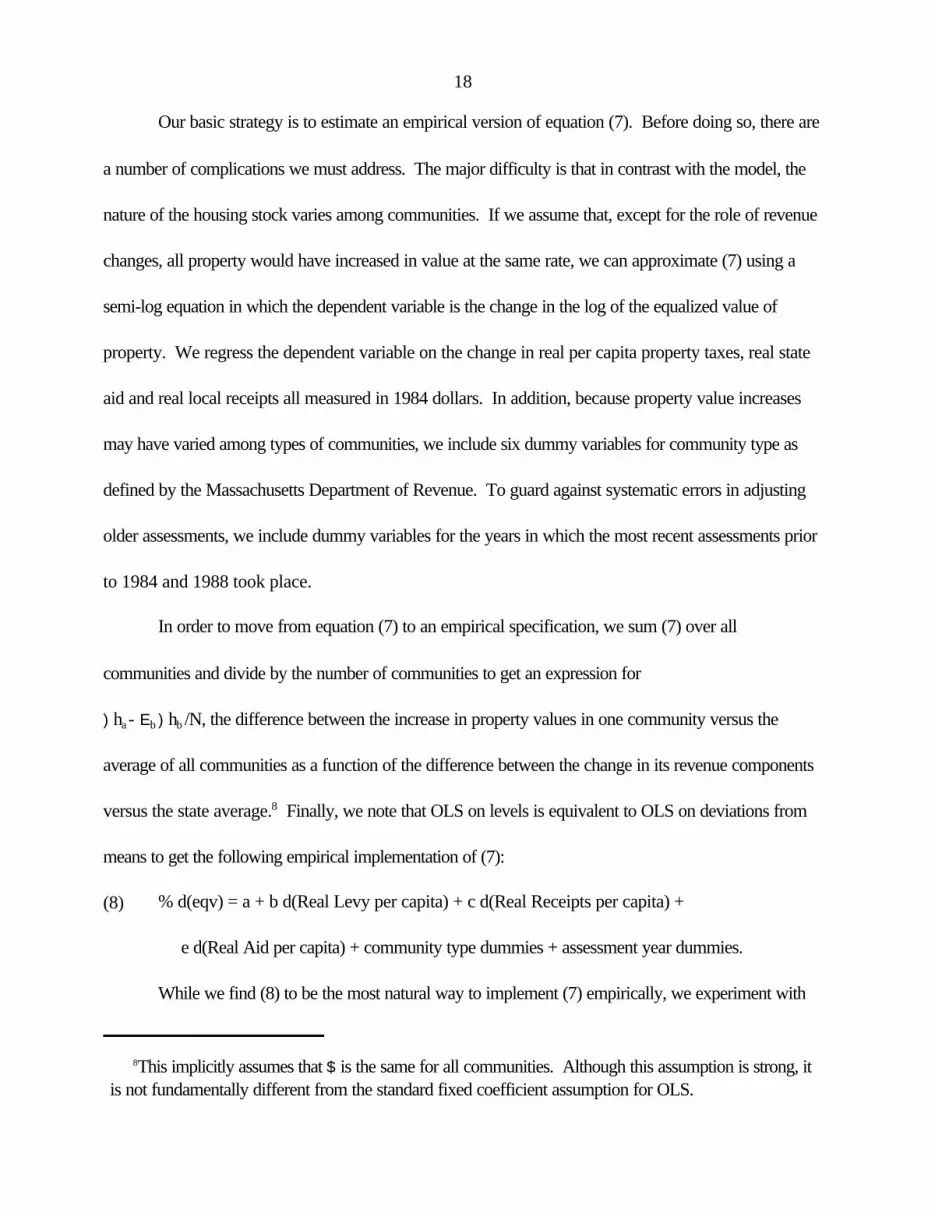
means to get the following empirical implementation of (7):

(8) % d(eqv) = a + b d(Real Levy per capita) + c d(Real Receipts per capita) +

e d(Real Aid per capita) + community type dummies + assessment year dummies.

While we find (8) to be the most natural way to implement (7) empirically, we experiment with

19

using the level of the equalized value as the dependent variable. When we do so, we regress the level of

equalized value on lagged equalized value as well as the remaining variables to capture the fact that, over

this period, the price of property grew at a rate well above the overall inflation rate.

The final issue we must address is endogeneity of the revenue variables. Since the state aid

formula explicitly relies on equalized value as one determinant, the change in state aid is clearly

endogenous. Formal tests confirm this.

Proposition 2½ largely eliminated the endogeneity of property tax revenues by initially forcing

some communities to reduce their tax rates and then by constraining the rate of growth of tax revenues.

More importantly, in contrast to the practice in many areas, it decouples tax revenue from property

values. When property values rise, the tax rate must be reduced to keep tax revenues constant except

for the permitted 2.5% growth rate. While not all communities were at their levy limit, over the period

we study housing prices were rising sufficiently rapidly that almost all communities would have exceeded

their levy limit if they did not adjust the tax rate. Thus there is no automatic relation between property

values and tax revenues.

There are three reasons that the tax levy may nevertheless still be endogenous. First,

communities are not required to collect all the tax revenues permitted by Proposition 2½, and some

choose not to. Secondly, the limit is adjusted for new development. New development will therefore

simultaneously raise tax revenues and equalized value. We experimented with using open space

(unimproved land) in 1984 as a proxy for development potential and including it in the equation.

However, preliminary estimates found no relation between open space and equalized value growth, and

we dropped this direction of inquiry. Finally, a community is allowed to exceed the restriction on the

growth of tax revenues (but not the restriction on the tax rate) by a vote of 50% of the participating

20

electorate. In the early years of Proposition 2½ such overrides were infrequent. Nevertheless, if

overrides are more likely when property values are rising, there may be a endogeneity problem. The

possibility of overriding means that the law might have been irrelevant. In fact, property taxes declined

and fees rose following passage of the law, suggesting that despite the override provision, the law was

binding. Moreover, Cutler, Elmendorf, and Zeckhauser (1997) report that between 1984 and 1990

overrides and exclusions added about .1% per year to the tax levy (with such votes being more common

towards the end of the period than towards the beginning). In addition, they find that

overrides/exclusions are less common when property values are rising, suggesting that failure to control

for the endogeneity of overrides creates a downward bias on the estimated impact of taxes on property

values, although this bias is likely to be small.

Similarly, local receipts may be endogenous if they respond to changes in property values.

While we have used local receipts as a proxy for fees, they include fines and motor vehicle excise tax

receipts (set at 2.5% by law). If people buy more or less expensive cars when the cost of property

increases, there may be an endogeneity problem.

We have a number of potential instruments. Between 1984 and 1988, state aid increased

rapidly and was aimed at those communities impacted most severely by Proposition 2½. We therefore

include measures of whether the community was constrained to cut taxes in 1982 and 1983 as potential

instruments. The severity of the cuts required by Proposition 2½ would be less in a community which

could lower its tax rate by moving to 100% assessment. We estimate the "true tax rate" as the tax levy

in 1981 divided by mean of the 1980 and 1982 equalized values. The true rate and its square are

potential instruments. Finally, the existence of open space may have allowed communities to avoid the

limits of Proposition 2½ by tailoring development to their needs. We experiment with the ratio of the

21

value of open space to other property values as an instrument. Our strategy is to treat the change in

state aid as endogenous and then test for the endogeneity of the two remaining revenue variables.

Descriptive statistics for key variables are given in Table 1. It is apparent that spending per

capita rose rapidly during this period even adjusted for inflation. This reflects the recovery from the

1982 recession and the booming economy of the Massachusetts miracle. Percentage increases in state

aid and fees were much more rapid than increases in the property tax levy.

Before turning to the results, it is important to note that they can only tell us about the impact of

changes in relative revenues among Massachusetts communities. Because all of the variation in the data

occurs within Massachusetts, we cannot address the impact of Proposition 2½ on the state as a whole.

It is possible that the law affected all communities positively or negatively (for example by increasing or

reducing the demand for labor across the state). Our work cannot address that issue directly.

IV. Results

The first column of Table 2 gives the results of estimating equation (8) treating the change in aid

as endogenous. The results are consistent with the theory if communities are constrained in their ability

to raise receipts to their optimal level. The effect of increases in state aid is statistically significant and

large in magnitude. The results suggest that a real increase in state aid of $100 per capita increases

property values by 49%. Increases in property taxes and in local receipts also have large and

statistically significant effects on property values. A $100 increase in property taxes per capita increases

property values by 27% while a comparable increase in fees raises property values by 21%. The

difference between the effect of property taxes and local receipts (mostly fees and fines) is plausible

given the tax-deductibility of property taxes. However, the estimates are too imprecise to allow us to

22

9This test consists of regressing the residuals from the structural equation on the first-stageregressors. N times the R2 from this auxiliary regression is distributed as a P2 with degrees of freedomequal to the number of over-identifying restrictions. It is equivalent to a test of whether adding theover-identifying regressors to the structural equation would change the results. This can be interpretedin at least two ways -- whether all choices of subsets of first-stage regressors would give the sameanswer or whether some of the first-stage regressors are correlated with the error term (conditional onthe others not being correlated with the error term).

conclude that property taxes are preferable to fees as theory suggests. The magnitude of the effect also

seems somewhat high, a point to which we return later.

The remainder of column (1) addresses two key issues. The first is whether the excluded first-

stage regressors have any explanatory power in the first-stage regressions. The F-test indicates that the

five excluded regressors are highly significant. However, visual inspection suggests that only the

variables measuring whether the community was constrained to lower property taxes in 1982 and 1983

actually provide identification. The second issue is whether the variables that are assumed to be

exogenous are correlated with the error term. The statistic for the Sargan-Basmann test of the over-

identifying restrictions is 8.07 well below standard significance levels for a P2(4).9

Nevertheless, there is reason for concern. If only two of the five first-stage regressors are

providing identification, then the presence of the remaining three first-stage regressors may be lowering

the power of the test. In column (2), we therefore present estimates using only the two variables

indicating the community was constrained to lower taxes as additional first-stage regressors. The

substantive results are effectively unchanged. The magnitude of the increase in the F-statistic confirms

that the remaining three variables had almost no explanatory power in the first-stage regression. The

Basmann-Sargan statistic falls to .25, well below its expected value of 1 with one degree of freedom.

Although the Basmann-Sargan test indicates that there is no need to be concerned about the

23

endogeneity of changes in the tax levy and local receipts, in column (3) we address directly the effect of

treating these variables as endogenous. For this estimation, we return to the original five excluded

variables used in the first column. While the F-statistic suggests that the five coefficients do not jointly

help to explain changes in receipts, this is somewhat misleading. Examination of individual equations (not

shown) reveals that aid responds to the constraints variables, the tax levy to the "true rate" in 1981 and

receipts to the availability of open space. The t-statistic on this last variable is just over 2 in the receipts

equation. We must therefore be somewhat guarded in our belief that we have adequate instruments, but

there is nevertheless reason to believe that the instruments are not excessively weak. The Basmann-

Sargan OID test is significant at the .1 level but not the .05 level. We conclude on the basis of the

results in the first three columns that there is reason to be concerned that either the true rate variables or

the open space variable is not a valid instrument although the results are not conclusive. We therefore

proceed with caution.

The main substantive result from column (3) is that when we treat all sources of revenue as

endogenous, the data are insufficient to provide us with any real insight. The impact of increases in the

tax levy essentially falls to zero. However, the standard error is sufficiently large that we cannot reject

the null that the coefficients in the first and third columns are the same. More formally, using a Durbin-

Hausman-Wu test, we fail to reject the exogeneity of the tax levy and receipts at any conventional level

of significance. We conclude that there is no strong evidence that we should treat receipts and taxes as

endogenous.

The fourth column addresses the issue of whether it is necessary to treat state aid as

endogenous. It is simultaneously a check on the power of the test and an exploration of an alternate

approach to estimation. One can think of the Basmann-Sargan test in this setting as a test of whether the

24

10All variables were obtained from the 1990 Census.

simultaneous equation system is recursive. There are thus six identifying assumptions -- that five

variables are excluded from the equalized value equation and that the covariance of the error terms in the

equalized value and aid equations is zero. Only one identifying assumption is necessary. The Basmann-

Sargan test statistic is 20.8, well above conventional significance levels. If we use only the two

constraint variables as excluded regressors, the test statistic is 10.8, which is again highly significant. We

conclude that it is necessary to treat aid as endogenous to changes in equalized value and that there is

reason to believe that our tests of exogeneity are reasonably powerful.

We prefer the sparse specification used in the previous columns. We believe that it is difficult to

be confident that most other community characteristics are exogenous to housing price. Nevertheless,

we recognize that it is possible that housing price changes are correlated with the revenue variable,

because of some sort of shift in tastes. For example, increasing income inequality may have increased

both spending and housing prices in more expensive communities. We believe that Proposition 2½

makes this implausible. However, in order to guard against this possibility, column (5) modifies the

specification of column (2) by adding controls for the educational and occupational make-up of the

community, income levels in the community and the age of the housing stock.10 Although the income and

education variables turn out to enter the equation significantly, it is evident that including these variables

has almost no effect on the parameters of interest. The coefficient on receipts falls somewhat and ceases

to be significant at the .05 level. The coefficient on state aid rises slightly while the coefficient on the levy

falls slightly. The F-test on the excluded first-stage regressors remains highly significant while the OID

test falls to .11.

25

Table 3 replicates Table 2 except that it uses all available communities. Columns (1) and (3) are

missing communities that had not conformed to the Classification Law by 1984 and thus did not have

information on the value of undeveloped land. The remaining columns use all 351 communities.

Superficially the results in Table 3 seem similar to those in Table 2 and, for some specifications,

possibly better. The estimated impact of increases in the levy falls but becomes more precise and

remains highly significant. Most importantly, the coefficient on local receipts falls to 0 as implied by the

theory. In some specifications, the impact of state aid is greater than in Table 2 where they already

seemed somewhat too high. However, in column (2) which was the preferred specification in Table 2,

the coefficient on state aid is similar in the two tables.

This superficial similarity is, in fact, misleading. The test of over-identifying restrictions in column

(1) rejects these restrictions. This raises the concern that either the levy or local receipts should be

treated as endogenous. A Durbin-Wu-Hausman test based on the estimates in column (3) confirms that

the levy although not local receipts should be treated as endogenous. Of course, the DWH test may

indicate endogeneity because one of the supposedly exogenous first-stage regressors is, in fact,

endogenous. Column (2) appears to provide support for this interpretation since when the set of first-

stage regressors is restricted, we cannot reject the over-identifying restrictions. However, the excluded

first-stage regressors have no explanatory power for the property tax levy. As a result, the OID test has

no power against correlation between the tax levy and the error term.

Taking these results together, we find a strong basis for concern that when we use the entire

sample, the tax levy should be treated as endogenous, evidence that supports our original sample

exclusion decisions. At the same time, the fact that the broad results for the full sample resemble those

for the restricted sample supports the view that our results are not driven by our sample selection

26

11The simplest reason is that communities typically set a tax rate per $1000 of valuation. If a tax rateof $10.00 would lead the community to exceed its levy limit, then it can only set a tax rate of $9.99

criteria.

The evidence from the OID and DWH tests suggests that, using our restricted sample, the tax

levy is not endogenous. Nevertheless, we consider this issue in greater detail. Endogeneity may arise for

at least three reasons. First, in many jurisdictions outside of Massachusetts the tax rate is not directly

affected by assessments. Increased assessments almost automatically increase tax revenue unless the

political authorities make a conscious decision to lower the tax rate. The combination of Proposition 2½

and the requirement that all properties by assessed at 100% of fair market value severed this link.

Second, since Proposition 2½ raises the levy limit in response to new growth, new growth can cause an

increase in the tax levy. By restricting the sample, we have attempted to eliminate this form of

endogeneity. The statistical analysis supports our view that we have been successful in this respect.

Finally, increased housing prices may increase the demand for public goods. Although overrides and

exclusions were relatively rare during the period we study, it is possible that property value increases

caused voters to support increased taxes. Our statistical tests should catch this source of endogeneity.

Even if they do not, Cutler, Elmendorf and Zeckhauser (1997) find that rising property values reduce

support for overrides/exclusions, thus suggesting that any bias is in the opposite direction.

As a final check, we further restrict the sample to ensure that we capture only exogenous

changes in the tax levy. In Table 4, we report the result of various sample restrictions. In each case, we

rely on the degree of excess taxing capacity. In principle, a constrained community should be at 100% of

its levy limit. However, practical factors may prevent the community from reaching this theoretical

maximum.11 We experiment with treating communities as constrained if they are within .1% or 1% of

27

which could leave it up to .1% below its levy limit. We chose the .1% level because it should eliminateshortfalls due to the number of digits problem with tax rates and 1% because discussions with financialadministrators indicated that other practical problems sometimes caused them to fall short of their levylimit, especially in the early years of Proposition 2½.

their levy limit. Unfortunately data on excess taxing capacity do not appear to be available prior to 1985.

In table 4, we treat communities as constrained if they were within the relevant range in either 1985 or

1988. The first and third columns impose that communities be within 1% and .1% of their levy limits

while the second and fourth columns also impose the data restrictions discussed in the data section.

All four estimates indicate that increases in the levy were associated with faster growth of

property values and that state aid had an even larger effect. The former effect is larger when the sample

is restricted as in Table 2. The estimated impact of changes in local receipts never reaches conventional

levels of significance.

So far we have used changes in equalized value of our measure of property values. We have

done so because we are concerned that assessed values may be unreliable. Prior to Proposition 2½

communities had an incentive to undervalue property. After 1979, they were prohibited by law from

doing so, and by 1984 most communities were in apparent conformity with the law. After Proposition

2½ communities that were constrained by 2½% tax limit had an incentive to over-assess property. Thus

we could easily find that those communities that reduced property taxes the most, also increased

assessments the most even if there were no real impact on property values.

Nevertheless, relying on equalized values has the disadvantage that it includes the value of

commercial and industrial property and open space. While we have restricted our sample to

communities with little residential growth, we cannot preclude the possibility that changes in equalized

value and the tax levy are positively correlated because commercial growth raises both.

28

Therefore in Table 5 we use the change in assessed residential property value as the dependent

variable. In addition, to the variables used in the previous specifications, we control for the change in

number of housing units between 1980 and 1990. This is never significant in the restricted sample as

would be expected since the communities in this sample experienced little new construction.

The first two columns in Table 5 replicate those in the first two columns in Table 2 except for the

change in dependent variable. The results are quite similar except that the positive impact of the

increases in the levy is somewhat attenuated using residential property values. This is consistent with

some bias being introduced by the inclusion of commercial property in equalized value. The excluded

first-stage regressors have almost no explanatory power for local receipts in this specification. Column

(3) resembles column (3) of Table 2 but treats the levy as endogenous but receipts as exogenous. The

results in columns (1) and (3) are almost identical except for the much higher standard errors that arise

when we treat the levy as endogenous. The results thus support our view that the change in the tax levy

can be treated as exogenous.

We do not present the results for the first three columns using the entire sample of 334

communities for which data on assessed values by property class are available. The results are similar to

those for the restricted sample except that the coefficient on local receipts is negative and statistically

significant. Using the full sample, the OID test rejects the choice of instruments for the specification with

all five excluded first-stage regressors. Visual inspection of the auxiliary regression used in the test

indicates that constrained to reduce taxes in 1983 is the source of the rejection. Column (4) gives the

results when the remaining first-stage regressors are used. The results are similar to those obtained in

Table 3. We note that for this specification, we simultaneously pass standard specification tests and

obtain reasonably precise estimates even though the tax levy is treated as endogenous. Again the results

29

reinforce our view that for this sample period the levy can be treated as exogenous.

The results in Table 5 indicate that our findings do not depend on our choice of equalized value

as our dependent variable. In Table 6, we return to using equalized value to provide some

additional tests of our specification. In all specifications we treat state aid as endogenous and use the

two variables measuring constraints as additional first-stage regressors. In columns (1) and (2) we treat

1988 nominal per capita equalized value as the dependent variable and include 1984 per capita

equalized value as an exogenous explanatory variable. In the first column, we do not constrain the

coefficients on the different years. We cannot reject the hypothesis that 1988 equalized value depends

only on 1984 equalized value and the real change in the three components of revenue.

In column (2), we therefore impose the constraint. The results are similar to those obtained in

table 2. Increases in all three components of revenue have a positive effect on property values. State

aid has the biggest effect followed by increases in the tax levy. However, the coefficient on state aid is

poorly determined and thus not statistically significant.

One advantage of the specification in column (2) is that it allows us to think more carefully about

the plausibility of the magnitude of the effects. A $1 increase in state aid must be worth at least $1

(ignoring the fact that a small fraction of the $1 comes from income taxes collected in the community).

The community could reduce fees by $1 and provide the same public services. If the community is

constrained, then it can use the increase in state aid to relax the constraint and receive a benefit valued at

more than $1. If the change in state aid is expected to be permanent, then the benefit should be

capitalized into the price of the house. If people discount the benefits at 5%, the estimate in column (2)

30

12Recall that the dependent variable is measured in $1988 while the explanatory variables are in$1984.

13Further evidence comes from the large sums of money contributed to campaigns intended tooverride Proposition 2½. Proponents of a $2.5 million override is one community with which we arefamiliar collected about $25,000 for their campaign. Donated time would bring the overall expenditureto well over $1 million.

suggests that $1 per year of state aid provides $3.63 per year of benefits.12 This appears somewhat high

to us but given the imprecision with which the coefficient is estimated is not unreasonable.13

One possible explanation for the high coefficients is that people interpreted the change from

1984 to 1988 not as a permanent change in the level but as an indicator of future rates of growth of

revenues. In the light of the booming Massachusetts economy, many communities expected state aid

and other revenue components to continue growing.

To cast light on this explanation, we repeat our analysis for the period 1984-1992. Given the

ups and downs experienced by the Massachusetts economy over this period, it is less likely that

individuals interpreted changes between 1984 and 1992 as indicators of future changes rather than new

levels. By 1992 most communities expected the growth of state aid and other revenues to be low.

Column (3) presents estimates for 1984-1992 that are analogous to those provided in table 2 for

the 1984-1988 period. We use the constraint variables and the true 1981 tax rate variables as first-

stage regressors. Preliminary tests rejected the exogeneity of the open space variables and indicated

that all four remaining first-stage regressors were required to create a powerful instrument. The F-test

on the four excluded regressors is 2.85. The Basmann-Sargan test-statistic is 6.32, well below its

critical value at the .05 level with three degrees of freedom.

The coefficients in column (3) are substantially smaller than those shown in the first two columns

31

of table 2. The impact of state aid is about half of that estimated for the 1984-1988 period and falls

short of statistical significance at conventional levels. The impact of increases in the tax levy is about

one-third of the estimate for the shorter period but remains highly significant. Both of these results are

consistent with the hypothesis that the relation between past growth and expected future growth declined

between 1988 and 1992. Finally, we note that the coefficient on receipts falls to zero, consistent with

the model outlined in the previous section. Perhaps communities learned how to avoid constraints on

fees or improved their ability to set them optimally.

Given that two studies (ours and Bradbury et al, 1996) obtain similar results for 1984-88 and

1990-94, it is natural to ask whether the findings would also apply to 1980-84 when the impact of

Proposition 2½ was arguably greatest and the change in tax levy plausibly most exogenous. Despite our

concerns about the uncertainty about the law in the aftermath of its passage and the quality of the

equalized value data for the earlier period, we attempt to replicate our study for 1982 to 1984 since we

can think of no valid instruments for the 1980 to 1982 period and equalized value is not available for

1981. We restrict the sample to the 199 communities that reassessed property in either 1981 or 1982 so

as to minimize that data quality issues. It is not, however, feasible, for reasons of sample size to further

restrict the sample.

We redefine the “true tax rate” as the 1981 tax levy/equalized value 1980, to avoid it being

correlated with the change in equalized value by construction. We use the true tax rate, its square and its

cube as identifying instruments. Because state aid depends on equalized valuations, we must continue to

instrument for changes in state aid. For this period, we must also be concerned about the potential

endogeneity of the tax levy. Since Proposition 2½ constrains the tax rate to be less than 2½%,

communities which otherwise would have been constrained by the tax rate cap were less constrained if

32

they experienced greater growth in property values. As a consequence, growth in property values could

affect the change in the tax levy over this period. However, by 1984 only 3 of the 199 communities were

constrained by the tax rate (although many were constrained by the levy limit); so this may not be an

important source of endogeneity.

Table 7 shows the results of this estimation. Note that all coefficients are multiplied by 1000

rather than the 100 used in tables 2-5. In the first column, only state aid is treated as endogenous while

in the second column both aid and the tax levy are endogenous. Given that the test of the over-identifying

restrictions falls well short of statistical significance, it is not surprising that the parameters are similar in

the two columns. At least when the levy is treated as exogenous, higher property tax increases (or

smaller declines) are associated with faster growth of equalized values. The estimated size of this effect

is, however, much smaller than for the 1984-1988 period. Moreover, the absence of a significant effect

of state aid is surprising as is the larger albeit imprecisely measured effect of local receipts.

The third and fourth columns of Table 7 address the issue of whether changes in revenues

associated with Proposition 2½ were anticipated and thus capitalized into housing prices by 1984. We

add the 1984-88 revenue changes to our specification. The results in column 3 show that future tax levy

changes were capitalized into housing prices. The effect of future state aid changes is large, negative and

very imprecisely measured, consistent with the view that the large state aid changes between 1984 and

1988 were not anticipated in 1984. The fourth column drops future state aid changes from the

specification. The results continue to strongly support a positive impact of the levy change on growth of

equalized value. The higher coefficient on future changes is somewhat surprising, but we cannot reject

the hypothesis that the coefficients on the 1982-84 and 1984-88 changes in levy are identical. Finally,

we cannot reject the hypothesis that changes in local receipts do not affect property values.

33

In sum, the results for 1982-84 confirm the results for 1984-88. Indeed they are in many ways

more plausible since the magnitudes of the effects are more consistent with our expectations.

Nevertheless, because of the data concerns raised earlier, we lean more heavily on the results from the

later period.

The results in Table 7 indicate that changes in property values are associated with the changes

that took place in the later period. This is consistent with the capitalization hypothesis. However, it is

also possible that the results merely capture a trend in property values that happens to be correlated with

revenue changes. Column (4) of Table 6 provides a final check on whether the specification is capturing

some other factors. In this column we replace equalized values for 1984-1988 (but not the revenue

variables) with values for 1976-1980. We then repeat the estimation of table 2 (column (2)). If our

revenue variables were capturing some other factor, then we might expect that they would also explain

growth of equalized value between 1976 and 1980. For example, if we were capturing communities on

the outer edge of Boston that were growing rapidly, we would expect relatively rapid growth over the

entire twelve year period. In fact, the results in column (4) of table 6 are quite different from the

previous estimates. The coefficients on the tax levy and receipts are effectively zero. While the growth

of state aid is associated with changes in equalized value between 1976 and 1980, the sign is the

opposite from that obtained for 1984-1988. We therefore conclude that our revenue components are

not mere proxies for fast-growing communities.

V. Discussion and Conclusion

Our results strongly suggest that communities that were able to increase revenues more rapidly in

the wake of the Proposition 2½ tax limit in Massachusetts experienced faster growth of property values.

Our results are thus consistent with a model in which communities seek to provide the desired level of

34

public services given constraints on their efficiency. Indeed our results for 1984-1992 fit such a model

almost perfectly.

Bradbury, Mayer and Case (1996) obtain similar results for the 1990-1994 period using a

model that closely resembles ours. Aside from the time period, the papers differ somewhat in their

emphasis. They concentrate on the effect of changes in the composition of expenditure while we focus

on changes in the structure of revenues. For reasons discussed above, it is impossible to identify

separately the impact of changes in revenues and expenditures. Our theoretical model assumes that the

distribution of expenditures is efficient given the level and composition of revenues. For purposes of the

empirical work, we could have assumed that the distribution of expenditures was independent of the

composition of revenues. In contrast, Bradbury et al examine the impact of the distribution of

expenditures on housing values. Implicitly, they also assume that the distribution of expenditures is

independent of the composition of revenues. Despite this difference in emphasis, our results are similar.

Both studies find that increased expenditure/revenue generally raised property values although the impact

differs across expenditure types or revenue sources.

Our findings underscore the importance of careful thought about the nature of endogeneity when

studying Proposition 2½. Vigdor (1998) is superficially very close to our work here and to Bradbury et

al. He regresses various measures of property value increase from 1980 to 1990 on the change in state

aid and the tax rate reduction required by Proposition 2½. We can interpret this specification as the

reduced-form of a system in which state aid is exogenous and the tax levy and local receipts are

endogenous. Yet both the formal link and the statistical evidence suggest that state aid must be treated as

endogenous. In contrast the case for changes in the tax levy being endogenous is weaker and that for

changes in local receipts quite weak. For the 1984-88 period, when we treat state aid as exogenous and

35

local receipts and the tax levy as endogenous, the coefficient on the tax levy is consistently negative and

sometimes statistically significant.

We conclude that the evidence is compelling that restrictions on a community’s ability to raise

taxes did lower its property values. This raises the immediate question as to why Massachusetts voters

supported Proposition 2½. In our view the most plausible explanation is that voters simply used the

wrong model. Many were convinced that taxes could be cut with only a negligible impact on public

services.

There are, however, alternative explanations. One is that voters foresaw that limiting property

taxes would shift taxation towards income taxes. For many voters this shift would have been desirable.

A second explanation is that the benefits and costs of taxation are distributed unequally. We are unable

to investigate whether tax limits help some classes of property such as expensive single-family homes.

Despite this caveat, our results are consistent with models of local public finance that emphasize

the importance of the role of local taxes in determining efficient levels of local public goods. They

suggest that tax limits may have severe adverse effects that are not anticipated by their proponents.

REFERENCES

Aaron, Henry J., Who Pays the Property Tax?, Washington, DC: Brookings Institution, 1975.

Bewley, Truman, “A Critique of Tiebout’s Theory of Local Public Expenditures,” Econometrica, 49(May 1981): 713-40.

Bradbury, Katharine, Mayer, Christopher J. and Case, Karl E., "Property Tax Limits and Local FiscalBehavior: Did Massachusetts Towns Spend Too Little on Town Services under Proposition 2½?"Federal Reserve Bank of Boston, unpublished, 1996.

Brueckner, Jan K., "Property Values, Local Public Expenditure, and Economic Efficiency," Journal ofPublic Economics, 11 (April 1979): 223-45.

36

Case, Karl E. and Grant, James H., "Property Tax Incidence in a Multijurisdictional Model," PublicFinance Quarterly, 19 (October 1991): 379-92.

Conley, John P. and Wooders, Myrna, "Anonymous Pricing in Public Goods Economies," University ofIllinois, Champaign, unpublished, 1997.

Cutler, David, Elmendorf, Douglas and Zeckhauser, Richard, “Restraining the Leviathan: Property TaxLimitation in Massachusetts,” FEDS Working Paper No. 1997-47, 1997.

Edel, Matthew and Sclar, Elliott, "Taxes, Spending, and Property Values: Supply Adjustment in aTiebout-Oates Model," Journal of Political Economy, 82 (Sept./Oct. 1974): 941-54.

Epple, Dennis, Filmon, Radu and Romer, Thomas, "Equilibrium among Local Jurisdictions: Toward anIntegrated Treatment of Voting and Residential Choice," Journal of Public Economics, 24 (August1984): 281-308.

Epple, Dennis, Zelenitz, Allan and Visscher, Michael, "A Search for Testable Implications of the TieboutHypothesis," Journal of Political Economy, 86 (June 1978), 405-25.

Ferguson, Ronald F., and Ladd, Helen F., "Massachusetts," in Fosler, R. Scott, ed., The NewEconomic Role of American States: Strategies in a Competitive World Economy, Oxford and NewYork: Oxford University Press, 1988: 19-87.

Gyourko, Joseph, and Tracy, Joseph, "The Structure of Local Public Finance and the Quality of Life,"Journal of Political Economy, 99 (August 1991): 774-806.

______, "On the Political Economy of Land Value Capitalization and Local Public Sector Rent-Seekingin a Tiebout Model," Journal of Urban Economics, 26 (September 1988): 152-73.

Hamilton, Bruce W., "Capitalization of Intrajurisdictional Differences in Local Tax Prices," AmericanEconomic Review, 66 (December 1976a): 743-53.

______, "The Effects of Property Taxes and Local Public Spending on Property Values: A TheoreticalComment," Journal of Political Economy, 84 (June 1976): 647-50.

Hobson, Paul, "The Incidence of Heterogeneous Residential Property Taxes," Journal of PublicEconomics, 29 (April 1986): 363-73.

Konishi, Hideo, "Voting with Ballots and Feet: Existence of Equilibrium in a Local Public GoodEconomy," Journal of Economic Theory, 68 (February 1996): 480-509.

Ladd, Helen F. and Bradbury, Katharine L., "City Taxes and Property Tax Bases," National TaxJournal, 41 (December 1988): 503-23.

37

______, and Wilson, Julie Boatright, "Why Voters Support Tax Limitations: Evidence fromMassachusetts' Proposition 2½," National Tax Journal, 35 (June 1982): 121-48.

Meadows, George Richard, "Taxes, Spending, and Property Values: A Comment and Further Results,"Journal of Political Economy, 84 (Part 1, August 1976): 869-80.

Mieszkowski, Peter, "The Property Tax: An Excise Tax or a Profits Tax?" Journal of Public Economics,1 (April 1972): 73-96.

Nechyba, Thomas J., “Existence of Equilibrium and Stratification in Local and Hierarchical TieboutEconomies with Property Taxes and Voting,” Economic Theory, 10 (1997): 277-304.

Oates, Wallace E. "The Effects of Property Taxes and Local Public Spending on Property Values: AnEmpirical Study of Tax Capitalization and the Tiebout Hypothesis," Journal of Political Economy, 77(Nov./Dec. 1969): 957-71.

Pollakowski, Henry O., "The Effects of Property Taxes and Local Public Spending on Property Values:A Comment and Further Results," Journal of Political Economy, 81 (July-August 1973): 994-1003.

Polinsky, A. Mitchell, and Daniel L. Rubinfeld, "The Long-Run Effect of a Residential Property Tax andLocal Public Services," Journal of Urban Economics, 5 (April 1978): 241-62.

Rosen, Kenneth T., "The Impact of Proposition 13 on House Prices in Northern California: A Test ofthe Interjurisdictional Capitalization Hypothesis," Journal of Political Economy, 90 (February 1982):191-200.

Scotchmer, Suzanne, "Public Goods and the Invisible Hands," in Quigley, John and Smolensky, Eugene,eds., Modern Public Finance, Cambridge, MA: Harvard University Press, 1994: 93-119.

Shenkel, William M., and Gaines, James P., "The Effect of Property Tax Variation on Housing Values,"Review of Business and Economic Research, 13 (Spring 1978): 80-91.

Taylor, Lori, "Government Budgets and Property Values," Federal Reserve Bank of Dallas EconomicReview, (September 1991): 1-7.

Tiebout, Charles M., "A Pure Theory of Local Expenditures," Journal of Political Economy, 64(October 1956): 416-24.

Vigdor, Jacob L., “Was Tiebout Wrong? Local Taxes and the Growth of Cities,” Harvard University,unpublished, 1998

Westhoff, Frank, "Existence of Equilibria in Economies with a Local Public Good," Journal of EconomicTheory, 14 February 1977): 84-112.

38

Zodrow, George R. and Mieszkowski, Peter, "The New View of the Property Tax: A Reformulation,"Regional Science and Urban Economics, 16 (August 1986): 309-27.

TABLE 1

DESCRIPTIVE STATISTICS

Mean Max Min Stan. Dev.

Constrained 1982 0.54 1.00 0.00 0.50

Constrained 1983 0.13 1.00 0.00 0.34

Per Capita Aid 1984 222.32 552.62 40.36 87.39

Per Capita Aid 1988 337.64 842.18 61.33 144.22

Per Capita Levy 1984 506.59 1145.36 135.40 196.90

Per Capita Levy 1988 632.66 1518.50 181.28 249.05

Per Capita Receipts 1984 112.16 1063.75 24.82 117.27

Per Capita Receipts 1988 178.23 1332.07 51.94 151.94

Equalized Value Per Capita 1984 26366.32 87151.71 10568.85 12452.36

Equalized Value Per Capita 1988 64153.53 191231.10 21392.63 29662.26

Certification Year

1982 0.34 1.00 0.00 0.47

1983 0.50 1.00 0.00 0.50

1984 0.33 1.00 0.00 0.47

1986 0.44 1.00 0.00 0.50

1987 0.37 1.00 0.00 0.48

1988 0.20 1.00 0.00 0.40

TABLE 2DETERMINANTS OF PERCENTAGE INCREASE IN EQUALIZED VALUE

(1984-1988)

(1) (2) (3) (4) (5)

)Levy/100 0.27 0.27 0.02 0.22 0.23(0.07) (0.07) (0.20) (0.05) (0.07)

)Aid/100 0.49 0.53 0.44 0.07 0.59(0.19) (0.20) (0.20) (0.05) (0.23)

)Receipts/100 0.21 0.22 0.51 0.19 0.14(0.09) (0.09) (0.47) (0.07) (0.09)

F-test excluded inst. Aid 3.55 8.78 8.78 - 6.10 Levy - - 3.81 - Receipts - - 1.22 -

OID test 8.07 0.25 5.49 20.8 0.91

______________________________________________________________________________Two-stage least squares estimates. The explanatory variables are expressed in real per capita terms. Allspecifications include six community type dummies and six dummies for the timing of the assessments. Standarderrors are in parentheses. Based on a sample of 178 Massachusetts communities.

(1) Aid endogenous, additional first-stage regressors -- constrained in 1982, constrained in 1983, true taxrate in 1981 and its square, open space ratio in 1984

(2) Aid endogenous, additional first-stage regressors -- constrained in 1982, constrained in 1983

(3) Aid, levy, receipts endogenous, additional first-stage regressors -- constrained in 1982, constrained in1983, true tax rate in 1981 and its square, open space ratio in 1984

(4) None endogenous, additional first-stage regressors for purposes of OID test -- constrained in 1982,constrained in 1983, true tax rate in 1981 and its square, open space ratio in 1984

(5) Same specification as (2) with median year housing was built, %high school graduates, %collegegraduates, %executives and professionals, %white collar, median family income and per capita income asadditional exogenous explanatory variables.

TABLE 3DETERMINANTS OF PERCENTAGE INCREASE IN EQUALIZED VALUE

(1984-1988)

(1) (2) (3) (4) (5)

)Levy/100 0.13 0.12 -0.06 0.11 0.10(0.03) (0.02) (0.07) (0.05) (0.02)

)Aid/100 0.94 0.52 0.46 0.09 0.84(0.25) (0.20) (0.27) (0.05) (0.35)

)Receipts/100 -0.13 -0.00 -0.22 0.08 -0.14(0.09) (0.07) (0.27) (0.05) (0.11)

F-test excluded inst. Aid 5.16 11.07 4.54 - 5.51 Levy - - 14.52 - Receipts - - 3.92 -

OID test 11.49 0.63 5.46 38.65 0.11

N 335 351 335 351 351______________________________________________________________________________Two-stage least squares estimates. The explanatory variables are expressed in real per capita terms. Allspecifications include six community type dummies and six dummies for the timing of the assessments. Standarderrors are in parentheses. For descriptions of specifications, see footnotes to Table 2.

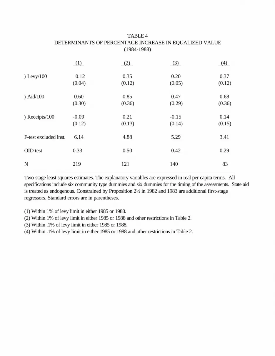
TABLE 4DETERMINANTS OF PERCENTAGE INCREASE IN EQUALIZED VALUE

(1984-1988)

(1) (2) (3) (4)

)Levy/100 0.12 0.35 0.20 0.37(0.04) (0.12) (0.05) (0.12)

)Aid/100 0.60 0.85 0.47 0.68(0.30) (0.36) (0.29) (0.36)

)Receipts/100 -0.09 0.21 -0.15 0.14(0.12) (0.13) (0.14) (0.15)

F-test excluded inst. 6.14 4.88 5.29 3.41

OID test 0.33 0.50 0.42 0.29

N 219 121 140 83______________________________________________________________________________Two-stage least squares estimates. The explanatory variables are expressed in real per capita terms. Allspecifications include six community type dummies and six dummies for the timing of the assessments. State aidis treated as endogenous. Constrained by Proposition 2½ in 1982 and 1983 are additional first-stageregressors. Standard errors are in parentheses.

(1) Within 1% of levy limit in either 1985 or 1988.(2) Within 1% of levy limit in either 1985 or 1988 and other restrictions in Table 2.(3) Within .1% of levy limit in either 1985 or 1988.(4) Within .1% of levy limit in either 1985 or 1988 and other restrictions in Table 2.

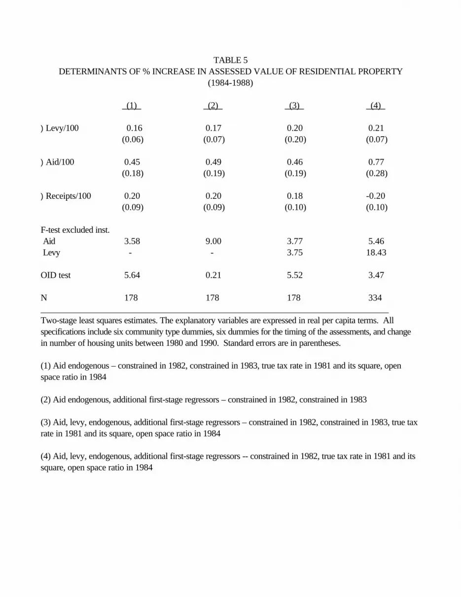
TABLE 5DETERMINANTS OF % INCREASE IN ASSESSED VALUE OF RESIDENTIAL PROPERTY

(1984-1988)

(1) (2) (3) (4)

)Levy/100 0.16 0.17 0.20 0.21(0.06) (0.07) (0.20) (0.07)

)Aid/100 0.45 0.49 0.46 0.77(0.18) (0.19) (0.19) (0.28)

)Receipts/100 0.20 0.20 0.18 -0.20(0.09) (0.09) (0.10) (0.10)

F-test excluded inst. Aid 3.58 9.00 3.77 5.46 Levy - - 3.75 18.43

OID test 5.64 0.21 5.52 3.47

N 178 178 178 334_____________________________________________________________________________Two-stage least squares estimates. The explanatory variables are expressed in real per capita terms. Allspecifications include six community type dummies, six dummies for the timing of the assessments, and changein number of housing units between 1980 and 1990. Standard errors are in parentheses.

(1) Aid endogenous – constrained in 1982, constrained in 1983, true tax rate in 1981 and its square, openspace ratio in 1984

(2) Aid endogenous, additional first-stage regressors – constrained in 1982, constrained in 1983

(3) Aid, levy, endogenous, additional first-stage regressors – constrained in 1982, constrained in 1983, true taxrate in 1981 and its square, open space ratio in 1984

(4) Aid, levy, endogenous, additional first-stage regressors -- constrained in 1982, true tax rate in 1981 and itssquare, open space ratio in 1984

TABLE 6

DETERMINANTS OF EQUALIZED VALUE 1984-1988 1984-1992 1976-1980 (1) (2) (3) (4)

)Levy 62.09 0.10 0.00(14.90) (0.03) (0.04)

)Aid 85.33 0.26 -0.27(64.52) (0.18) (0.11)

)Receipts 58.30 0.00 -0.05 (21.60) (0.02) (0.05)

Levy 1988 74.24 (51.25)

Levy 1984 -61.59 (42.19)

Aid 1988 169.65(484.61)

Aid1984 -241.15(742.78)

Receipts 1988 42.26 (25.74)

Receipts 1984 -47.03 (32.26)

Equalized Val. 2.07 2.261984 (0.51) (0.14)

OID test - 0.33 6.32 0.09______________________________________________________________________________2SLS estimates with aid endogenous and constrained in 1982 and in 1983 as additional first-stage regressors.In (3) the true 1981 tax rate and its square are also used. Explanatory variables are expressed in real per capitaterms. All specifications include six community type dummies and six dummies. Standard errors are inparentheses. In columns (3)- (4) coefficients are multiplied by 100. (1), (2) Dependent variable - nominalequalized value per capita. (3)- (4) Dependent variable - percent change in equalized value per capita.

TABLE 7

DETERMINANTS OF PERCENTAGE EQUALIZED VALUE GROWTH(1982-1984)

(1) (2) (3) (4) )Levy 81-84 0.11 0.13 0.18 0.14

(0.05) (0.19) (0.07) (0.05)

)Aid 81-84 -0.07 -0.08 1.29 0.71(0.37) (0.41) (0.68) (0.43)

)Receipts 81-84 0.31 0.34 -0.11 0.03(0.20) (0.33) (0.28) (0.21)

)Levy 84-88 0.31 0.27 (0.09) (0.07)

)Aid 84-88 -1.45

(1.10)

)Receipts 84-88 0.78 0.28 (0.42) (0.15)

OID test 3.20 3.18 >0.01 2.65______________________________________________________________________________All coefficients are multiplied by 1000. 2SLS estimates with aid (and levy in column (2)) endogenous andlevy81/equalized value 1980, its square and its cube as identifying first-stage regressors. All specificationsinclude six community type dummies and three dummies for the timing of the assessments. Sample restricted to199 communities with revaluations in 1981 or 1982. Standard errors are in parentheses.