A Fourier Spectral Method forHomogeneous Boltzmann Equations

Lorenzo PARESCHI(∗) and Benoit PERTHAME(∗∗)

(*) Dipartimento di Matematica, Universita di BolognaPiazza Porta S. Donato 5, 40127 Bologna, Italy

(**) Universite Paris 6 et CNRS, Laboratoire d’Analyse NumeriqueBC 187, 4 place Jussieu, 75252 Paris Cedex 05, France

andINRIA-Rocquencourt, MENUSIN, B.P. 105, 78153 Le Chesnay Cedex, France

Abstract

A numerical method for the solution of the spatially homogeneous Boltzmannequation is proposed. The scheme is based first in expanding the distribution func-tion in Fourier series, then in finite difference discretizing in time and velocity space.This allows an accurate evaluation of the collision operator with a reduced com-putational cost. Moreover, for a class of collision kernels, this approach leads to aquadrature formula that can be computed through a fast algorithm. First resultson a twodimensional problem confirm the efficiency of the method.

1. Introduction

The Boltzmann equation describes the temporal evolution of the one particle

distribution function f = f(x,v, t), being t the time, x the position and v the

velocity of particles, in a gas of molecules interacting through binary collisions

[Ce], [TM]. The rate of change of the distribution function is governed by a

balance of free streaming of particles in space, and of relaxation to equilibrium

due to collisions.

Schemes based on splitting the physical processes of streaming and relax-

ation are widely used, both in stochastic as in deterministic methods, to solve

numerically the Boltzmann equation. Due to the large number of integration

1

variables in the collision term and to the stiffness of this term near the fluid

regime the main difficulties rely in the approximation of the relaxation process.

This is usually achieved by means of random particle methods [Bi], [Pe], [Na],

which essentially are based on a particle approximation of the densities as a sum

of Dirac masses and on a random integration of the collision operator. These

methods, because of the Monte Carlo procedure, are expensive for unsteady

flows and always present fluctuating results. On the other hand the high cost of

deterministic methods [MRS], [Mo] make these schemes usable only in physical

situations that do not require a large number of point in the velocity field to

approximate correctly the solution.

The goal of the paper is to develop a numerical method for the collision

phase which presents the characteristics of accuracy typical of spectral ap-

proaches but with a reduced computational cost. Our method is derived di-

rectly from the continuous Boltzmann equation by representing the solution to

the problem as a truncated Fourier series (a similar idea have been explored in

[GM],[GP] in a different way). For general kernels this approach leads to an ’ex-

act’ numerical scheme that can be computed with a first reduction in the cost.

In particular, for the class of models, which are referred to as Maxwell models,

with an energy independent collision rate we derive an approximation formula

that can be evaluated through a fast algorithm.

In the next paragraphs we describe the main characteristics of the approx-

imation of the relaxation phase in Fourier variables and discuss a first bidimen-

sional test case.

2. The collision phase

The collision phase is characterized by the spatially homogeneous Boltz-

mann equation ⎧⎨

⎩

∂f

∂t=

1

ϵQ (f, f)

f(x,v, t = 0) = f0(x,v)(2.1)

2

being Q(f, f) the bilinear collision operator

Q(f, f) =

∫

IR3×S2

β(g · ng

, g)[f(v′)f(w′)− f(v) f(w)]dwdn. (2.2)

In the above expressions ϵ is the Knudsen number, g = v − w is the relative

velocity and v′ and w′ are the post-collision velocities given by

v′ = (v +w)/2 + gn/2, w′ = (v +w)/2− gn/2.

Let us remark that in (2.1) the definition domain of the distribution function f

is the velocity space IR3 whereas the variable x acts as a parameter.

During the evolution process, Boltzmann’s collision operator preserves local

mass, momentum and energy∫

IR3

Q(f, f)(v)(1,v, v2)dv = (0, 0, 0). (2.3)

The first problem that one has to deal with is the fact that a numerical ap-

proximation to (2.1) requires the initial given density f0 in a compact support

whereas the steady state solution is a local Maxwellian that clearly does not have

this property. As a consequence of this, relations (2.3) are no longer verified in

a bounded domain. To avoid this fact previous authors proposed to modify the

collision mechanics in order to satisfy the conservation laws.

Here we consider a more natural approach to the problem for a distribution

function f with supp(f(v)) ⊂ BR, where BR is the ball of radius R centered in

the origin. From the conservation of energy

(v′)2 + (w′)2 = v2 + w2 ≤ 2R2

and hence v′, w′ ≤√2R.

This implies that the collision operator has compact support with

supp(Q(f, f)(v)) ⊂ B√2R.

In order to write a scheme for the approximation of (2.2) we define the

distribution function f(v) on the cube

C(2+√2)R = [−(2 +

√2R), (2 +

√2R)]3

3

by assuming {f(v) = 0 on C(2+√

2)R \ BR

f(v) = f(v) onBR.(2.4)

The following proposition holds:

Proposition 2.1: Let supp(f(v)) ⊂ BR and f defined by (2.4), then we have

Q(f, f) =

∫

BR×S2

β[f(v′)f(w′)− f(v)f(w)]χ(g ≤ 2R)χ(v ≤√2R)dwdn (2.5)

where χ(·) is the indicator function.

Proof:

Indeed

(i) If v′,w′ ∈ BR, then

g = |v −w| = |v′ −w′| ≤ 2R

thus χ(g ≤ 2R) = 1, and also

v2 ≤ v2 + w2 = (v′)2 + (w′)2 ≤ 2R2

hence v ≤√2R and χ(v ≤

√2R) = 1.

(ii) If v′ (or w′) ∈ C(2+√2)R \ BR, then

f(v′) = 0 (or f(w′) = 0),

and (2.5) is clear.

(iii) If v′ and w′ ∈ C(2+√2)R then

χ(v ≤√2R)χ(g ≤ 2R) = 0

and again (2.5) is true.

Otherwise v ≤√2R, g ≤ 2R implies

v′ = (v +w)/2 + gn/2 = v + (gn− g)/2

4

thus v′ ≤ v + g ≤ (2 +√2)R which contradicts the assumption (iii).

By virtue of this result the problem of the evaluation of f has been reduced

to a bounded domain (time dipendent) adapted for numerical methods and in

which the fundamental properties of the Boltzmann equation still hold.

3. A Spectral Approximation

Let us consider the distribution function f extended by periodicity to a

periodic function on CT = [−T, T ]3, T = (2 +√2)R.

The approximation function fN on CT is sought in the form of the truncated

Fourier series [CHQZ]

fN (v) =N∑

h=−N

φheiv·hπ/T

φh =1

(2π)3

∫

[−T,T ]3f(v)e−iv·hπ/Tdv

(3.1)

where in (3.1) for simplicity of notations we used a single index for the three-

dimensional sum over the vector h.

Now by substituting expression (3.1) in (2.2) we obtain

Q(fN , fN)(v) =N∑

h,k=−N

φhφk

∫β{eiv

′·hπ/T eiw′·kπ/T − eiv·hπ/T eiw·kπ/T }χ(g ≤ 2R)χ(v ≤

√2R)dwdn

(3.2)

=N∑

h,k=−N

φhφkeiv·(h+k)π/T βR(h,k). (3.3)

We have set

βR(h,k) =

∫β{ei(gn·(h−k)−g·(h+k))π/2T − e−ig·kπ/T }χ(g ≤ 2R)dgdn (3.4)

5

Now it is remarkable that (3.4) is a scalar quantity completely independent on

the function fN and on the argument v, depending just on the particular kernel

structure and on the radius R. Moreover the following holds:

Proposition 3.1: βR(h,k) is a function of |h−k|, |h+k| and (h−k) · (h+k).

Remark: This proposition can be useful because, in a numerical method, the

βR(h,k) are stored and it explains how to diminish the information to be saved.

Proof:

Set

g = gm, h+ k = |h+ k|l1, h− k = |h− k|l2.

Then

βR(h,k) =

∫β(m · n, g){eigλ(n·l2µ

−1−m·l1µ)π/2T

− eigλ(m·l2µ−1−m·l1µ)π/2T }χ(g ≤ 2R)gdgdmdn

(3.5)

with

λ =1

2(|h− k|)1/2(|h+ k|)1/2, µ = (|h− k|)−1/2(|h+ k|)1/2.

Now by noting with Φ(l1, l2) the quantity (3.5) as a function of l1 and l2 we

have

Φ(l1, l2) = Φ(R · l1, R · l2)

for any unitary transform R (rotation or symmetry) of IR2.

In complex notation l1 = eiθ1 ,l2 = eiθ2 , R = e±iθ. Choosing R = e−iθ2

Φ(eiθ1 , eiθ2) = Φ(ei(θ1−θ2), 1)

= Ψ(ei(θ1−θ2))

= Ψ(e−i(θ1−θ2)).

Thus

Φ(l1, l2) = Ψ(cos(θ1 − θ2)) = Ψ(l1 · l2).

6

Finally by rewriting equation (3.3) in the form

Q(fN , fN)(v) =N∑

l=−N

Qleiv·lπ/T

Ql =N∑

h,k=−Nh+k=l

φhφk βR(h,k).

(3.6)

we can state the following:

Proposition 3.2: Let f(v) be a distribution function with compact support

expanded in Fourier series as in (3.1). Then Q(fN , fN)(v) can be computed

exactly with O(N2) operations, being N the total number of Fourier coefficients.

Remark: The usual cost for a method based on N parameters is O(N2M)

where M >> 1 is the angle discretization.

4. Maxwellian kernels

Therefore, the implementation of (3.6) is reduced to calculating and storing

just once integrals like (3.4). For the general situation these terms are a huge

number depending on the characteristics of β.

In particular, for Maxwellian kernels, β = β(g·ng ), that is for particles inter-

acting with a collision rate independent on the relative velocity, as R → ∞, Ql

concentrates on a circle for each l.

In fact, for these molecules, the gain part of the collision operator can be

written in the form

Q+(f, f) =

∫

IR3

∫

{h·k=0}β(

(h− k)

|h− k|· (h+ k)

|h+ k|)Φ(h)Φ(k)

|h− k|2ev(h+k)dkdh. (4.1)

Here Φ denotes the usual Fourier transform [Bo].

This does not make much sense for a general periodic function, but it sug-

gests that in this limit formula (3.6) can be reduced to the vectors h,k with

h · k = 0. Thus a good approximation of (3.6) is given by

Ql ≃N∑

h,k=−Nh+k=lh·k=0

φhφk β∞(h,k), (4.2)

7

which means a computational cost ofO(N logN). In fact (3.6a) can be evaluated

through the classical FFT algorithm whereas the orthogonality relation reduces

the number of operations in (3.6b) from N2 to N logN .

To conclude this section we observe that the macroscopic quantities, mass,

momentum and energy are defined by means of the Fourier coefficients as

ρ(t) = (2T )3φ0(t)

u(t) =N∑

h=−N

φhG(h)

e(t) =N∑

h=−N

φhL(h)

(4.3)

where

G(h) =1

(2T )3

∫

[−T,T ]3vei2πhv/Tdv

L(h) =1

(2T )3

∫

[−T,T ]3v2ei2πhv/Tdv.

(4.4)

These functions vanish except on the three orthogonal axes in the frequency

space defined by hx = 0, hy = 0 and hz = 0.

5. Numerical results

In order to test the validity of the method we have considered a bidimen-

sional problem for a Maxwellian gas. For the time discretization of (2.1) we use

the first order scheme proposed in [GPT] which has good properties of accuracy

and stability. The practical implementation is performed by using the FFT al-

gorithm for the computation of the Fourier coefficients on a 32× 32 points grid.

Due to approximations, formula (4.2) is no more conservative in momentum and

energy (mass is preserved). We note that coefficients G(h), and L(h) have a

highly oscillating behaviour which strongly damps with h. In particular, by

analogy with the previous remark, in the limit situation as R → ∞ equations

(3.9b-c) collapse to the values of the gradient and the Laplacian of the Fourier

transform at the origin.

8

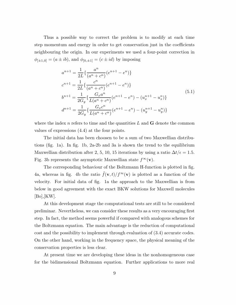
Thus a possible way to correct the problem is to modify at each time

step momentum and energy in order to get conservation just in the coefficients

neighbouring the origin. In our experiments we used a four-point correction in

φ[±1,0] = (a± ib), and φ[0,±1] = (c± id) by imposing

an+1 =1

2L{ an

(an + cn)(en+1 − en)}

cn+1 =1

2L{ cn

(an + cn)(en+1 − en)}

bn+1 =1

2Gy{ Gxan

L(an + cn)(en+1 − en)− (un+1

x − unx)}

dn+1 =1

2Gy{ Gxcn

L(an + cn)(en+1 − en)− (un+1

y − uny )}

(5.1)

where the index n refers to time and the quantities L and G denote the common

values of expressions (4.4) at the four points.

The initial data has been choosen to be a sum of two Maxwellian distribu-

tions (fig. 1a). In fig. 1b, 2a-2b and 3a is shown the trend to the equilibrium

Maxwellian distribution after 2, 5, 10, 15 iterations by using a ratio ∆t/ϵ = 1.5.

Fig. 3b represents the asymptotic Maxwellian state f∞(v).

The corresponding behaviour of the Boltzmann H-function is plotted in fig.

4a, whereas in fig. 4b the ratio f(v, t)/f∞(v) is plotted as a function of the

velocity. For initial data of fig. 1a the approach to the Maxwellian is from

below in good agreement with the exact BKW solutions for Maxwell molecules

[Bo],[KW].

At this development stage the computational tests are still to be considered

preliminar. Nevertheless, we can consider these results as a very encouraging first

step. In fact, the method seems powerful if compared with analogous schemes for

the Boltzmann equation. The main advantage is the reduction of computational

cost and the possibility to implement through evaluation of (3.4) accurate codes.

On the other hand, working in the frequency space, the physical meaning of the

conservation properties is less clear.

At present time we are developing these ideas in the nonhomogeneous case

for the bidimensional Boltzmann equation. Further applications to more real

9

computations will depend upon the possibility to extend a formula like (4.2) to

more general collision kernels.

Acknowledgement

L. Pareschi would like to thank the INRIA, MENUSIN, at Rocquencourt

for its kind hospitality during his visits there.

References

[Ce]. C. Cercignani, Theory and application of the Boltzmann equation, Springer

Verlag, New York (1988).

[CHQZ]. C. Canuto, M.Y. Hussaini, A. Quarteroni, T.A. Zang, Spectral methods in

fluid dynamics, Springer Verlag, New York (1988).

[Bi]. G.A. Bird, Molecular gas dynamics, Clarendon Press, Oxford, (1994).

[Bo]. A.V. Bobylev, The theory of the nonlinear spatially uniform Boltzmann

equation for Maxwell molecules, Soviet Scient. Rev. C,20, (1988), 111-233.

[GM]. Y.N. Grigoriev, A.N. Mikhalitsyn, A spectral method of solving Boltzmann’s

kinetic equation numerically, U.S.S.R. Comp. Math. Phys., 23, 6, (1983),

105-111.

[GP]. E. Gabetta, L. Pareschi, The Maxwell gas and its Fourier transform towards

a numerical approximation, Series on Advances in Math. for App. Scie.,

23, (1994), 197-201.

[GPT]. E. Gabetta, L. Pareschi, G. Toscani, Wild sums and numerical approxima-

tion of Boltzmann equation, Pubblicazioni IAN di Pavia, N.941, 1994.

[KW]. M. Krook, T. T. Wu, Phys. Rev. Lett. 36, (1976), 1107.

[Mo]. Y. Morchoisne, Une methode de differences finies pour la resolution de l’e-

quation de Boltzmann: Traitment du terme de collision, C. R. Acad. Sci.

313, Serie II, (1991), 1513-1518.

10

[MRS]. Y.L. Martin, F. Rogier, J. Schneider, Une methode deterministe pour la

resolution de l’equation de Boltzmann inhomogene, C. R. Acad. Sci. 314,

Serie I, (1992) 483-487.

[Na]. K. Nambu, Direct simulation scheme derived from the Boltzmann equation.

I. Monocomponent Gases, J. Phys. Soc. Japan, 52, (1983), 2042-2049.

[Pe]. B. Perthame, Introduction to the theory of random particle methods for

Boltzmann equation, in Advances in Kinetic Theory and Computing, B.

Perthame Editor, World Scientific, 1994.

[TM]. C. Truesdell, R.C. Muncaster, Fundamentals of Maxwell’s kinetic theory of

a simple monoatomic gas, Academic Press, New York (1980).

11

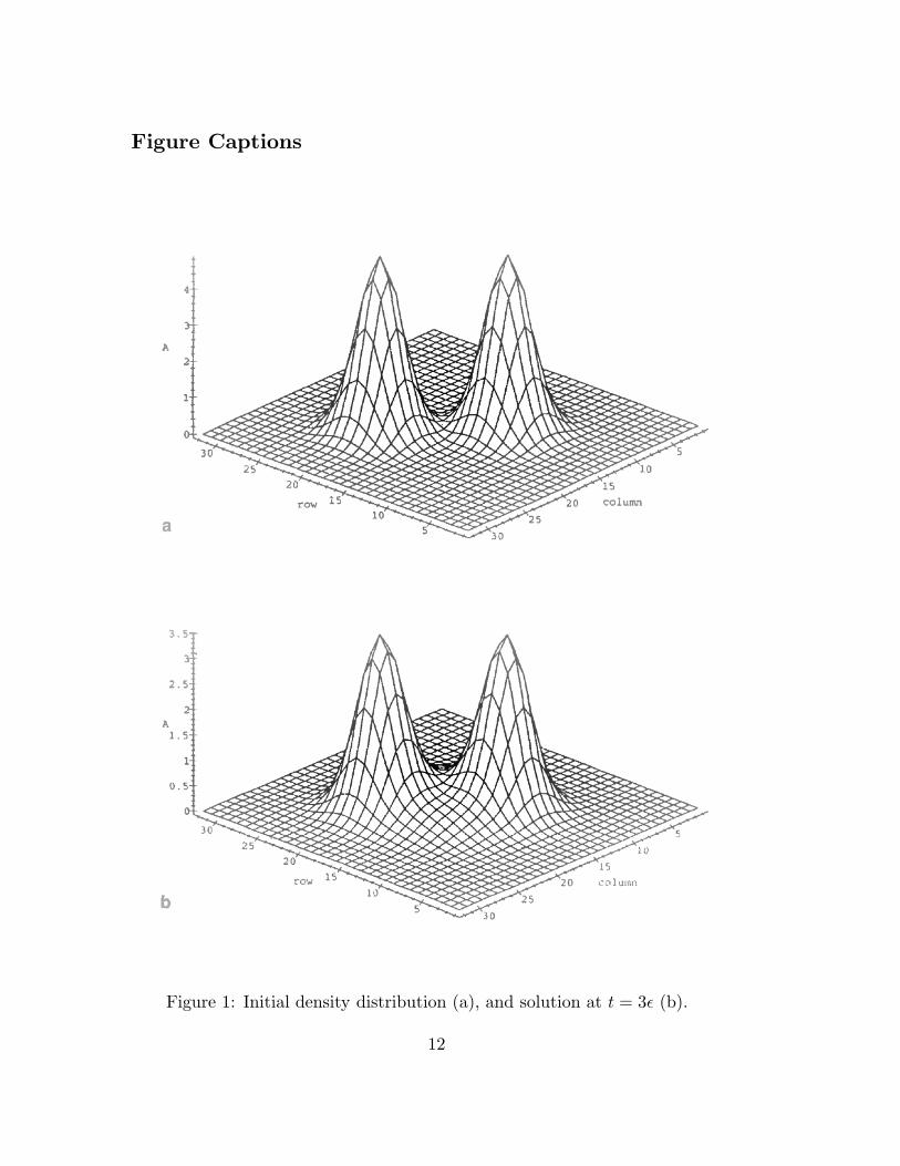
Figure Captions

Figure 1: Initial density distribution (a), and solution at t = 3ϵ (b).

12

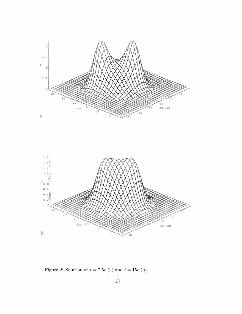
Figure 2: Solution at t = 7.5ϵ (a) and t = 15ϵ (b).

13

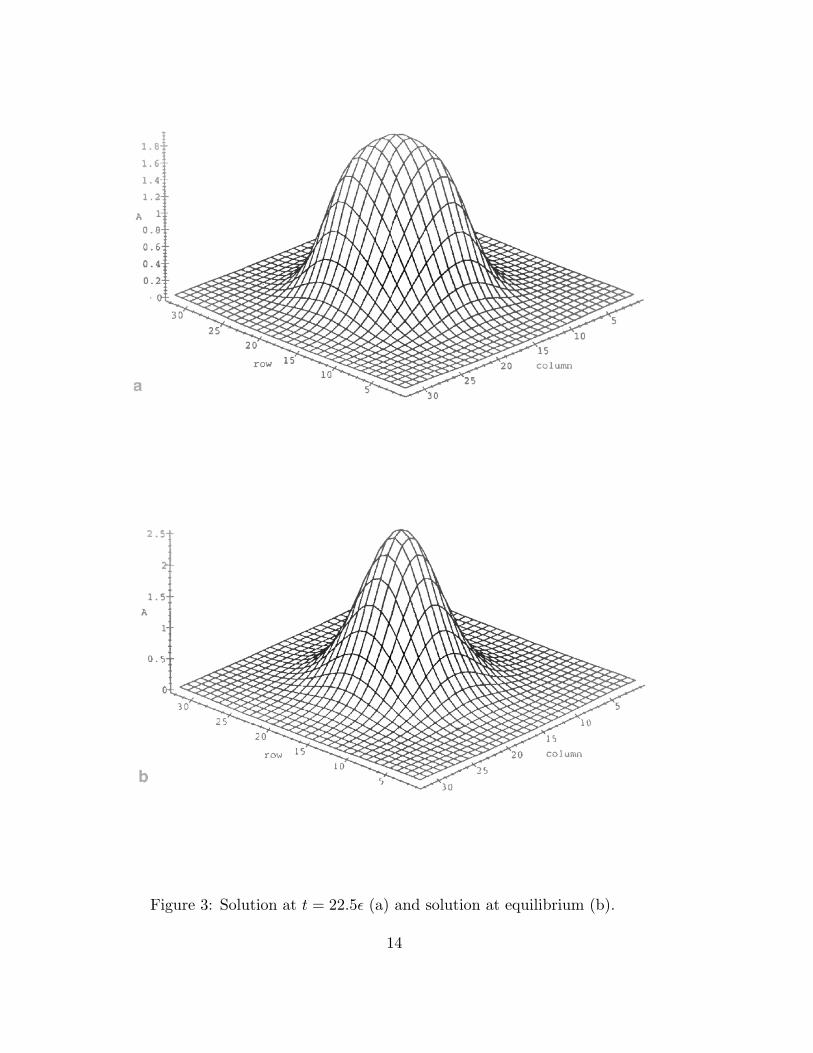
Figure 3: Solution at t = 22.5ϵ (a) and solution at equilibrium (b).

14

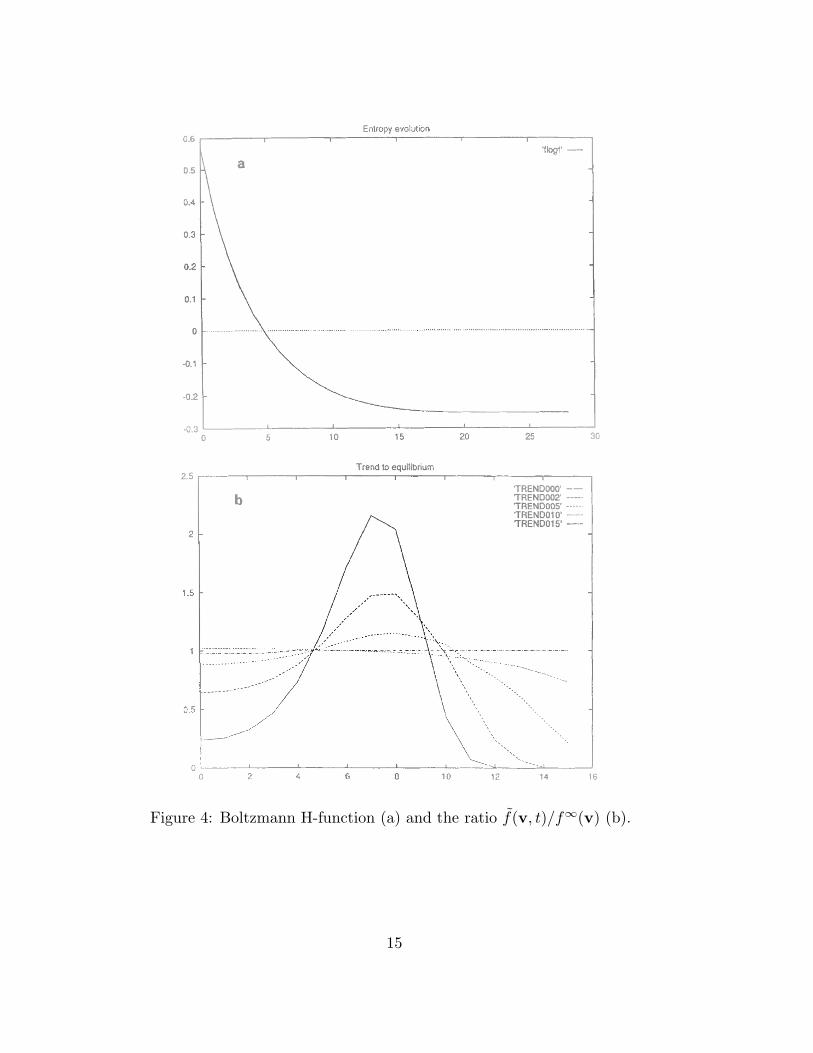
Figure 4: Boltzmann H-function (a) and the ratio f(v, t)/f∞(v) (b).

15