1

A global hydrological simulation to specify the sources of water used by humans

Naota Hanasaki12, Sayaka Yoshikawa3, Yadu Pokhrel4, Shinjiro Kanae3 1 National Institute for Environmental Studies, Tsukuba, Japan 5 2 International Institute for Applied System Analyses, Laxenburg, Austria 3 Department of Civil and Environmental Engineering, Tokyo Institute of Technology, Tokyo, Japan 4 Department of Civil and Environmental Engineering, Michigan State University, East Lansing, USA

Correspondence to: Naota Hanasaki (hanasaki@nies.go.jp)

10

Abstract. Humans abstract water from various sources to sustain their livelihood and society. Some global hydrological

models (GHMs) include explicit schemes of human water abstraction, but the representation and performance of these schemes

remain limited. We substantially enhanced the water abstraction schemes of the H08 GHM. This enabled us to estimate water

abstraction from six major water sources, namely, river flow regulated by global reservoirs (i.e., reservoirs regulating the flow

of the world’s major rivers), aqueduct water transfer, local reservoirs, seawater desalination, renewable groundwater, and 15

nonrenewable groundwater. In its standard setup, the model covers the whole globe at a spatial resolution of 0.5° × 0.5°, and

the calculation interval is one day. All the interactions were simulated in a single computer program and all water fluxes and

storage were strictly traceable at any place and time during the simulation period. A global hydrological simulation was

conducted to validate the performance of the model for the period of 1979-2013 (land use was fixed for the year 2000). The

simulated water fluxes for water abstraction were validated against those reported in earlier publications, and showed a 20

reasonable agreement at the global and country level. The simulated monthly river discharge and terrestrial water storage

(TWS) for six of the world’s most significantly human-affected river basins were compared with gauge observations and the

data derived from the Gravity Recovery and Climate Experiment (GRACE) satellite mission, respectively. It is found that the

simulation including the newly added schemes outperformed the simulation without human activities. The simulated results

indicated that, in 2000, of the 3628±75 km3yr-1 global freshwater requirement, 2839±50 km3yr-1 was taken from surface water 25

and 789±30 km3yr-1 from groundwater. Streamflow, aqueduct water transfer, local reservoirs, and seawater desalination

accounted for 1786±23, 199±10, 106±5, and 1.8±0 km3yr-1 of the surface water, respectively. The remaining 747±45 km3yr-1

freshwater requirement was unmet, or surface water was not available when and where it was needed in our simulation.

Renewable and nonrenewable groundwater accounted for 607±11 and 182±26 km3yr-1 of the groundwater total, respectively.

Each source differed in its renewability, economic costs for development, and environmental consequences of usage. The 30

model is useful for performing global water resource assessments by considering the aspects of sustainability, economy, and

environment.

2

1. Introduction

Water is an indispensable resource for human society. The securing of water resources is an important global challenge in the

21st century, because the demand for water is projected to increase due to the growing population, increased economic activity,

and changing climate (Oki and Kanae, 2006). To quantify global water availability and use in the past, present, and future, a

number of global hydrological models (GHMs) have been developed to provide an explicit representation of human water use, 5

including H08 (Hanasaki et al., 2008a,b, 2010), WaterGAP (Alcamo et al., 2003; Döll et al., 2003, 2012, 2014), LPJmL

(Gerten et al., 2004; Rost et al., 2008, Biemans et al., 2011), PCR-GLOBWB (van Beek et al., 2011; Wada et al., 2011, 2014),

WBMplus (Vörösmarty et al., 1989; Wisser et al. 2010), HiGW-MAT (Pokhrel et al., 2012a,b, 2015), and others. The history

of model development is well summarized in Nazemi and Wheater (2015a,b), Bierkens (2015), Sood and Smakhtin (2015), and

Pokhrel et al. (2016). 10

The fundamental objectives of GHMs are twofold. The first objective is to estimate flows and stocks of natural hydrological

components (e.g., river water, soil moisture, and groundwater) and human water use at sufficiently high spatial and temporal

resolution. This objective has been largely achieved in the last two decades by developing physical hydrological models to

solve the surface water balance (e.g., Döll et al., 2003; Gerten et al., 2004; Hanasaki et al., 2008a; van Beek et al., 2011),

developing water use models to estimate irrigation, industrial, municipal, and other water requirements (e.g., Döll and Siebert, 15

2002; Alcamo et al., 2003; Rost et al., 2008; Hanasaki et al., 2008b, Wada et al., 2011; Flörke et al., 2013), and developing

global gridded data to provide the boundary conditions of such models (e.g., Döll et al., 2003; Siebert et al., 2005; Lehner et al.,

2011). The second objective is to represent the interaction between natural hydrology and human water use within a single

modeling framework. Water abstraction from rivers was first implemented in GHMs (e.g., Hanasaki et al., 2008b; Rost et al.,

2008). This enabled the GHMs to represent the fundamental nature-human interactions, in which upstream water abstraction 20

reduces water availability in downstream areas.

One of the remaining challenges of GHMs is to enable water abstraction from various water sources including the effects of

water infrastructure. Water sources can be separated into surface water and groundwater. Groundwater is a renewable water

source, but it could be depleted if the volume of water abstraction exceeds the recharge (e.g., Wada et al., 2010). Hence it

should be further separated into renewable and nonrenewable (overexploited) categories. River flow has been the dominant 25

surface water source for humans since ancient times. Because river flow has substantial temporal variations, it is regulated and

stored in artificial reservoirs and ponds, which can be used in periods of low flow. Furthermore, because river flow is

accessible to regions located along the channel, aqueducts have been constructed to transfer it to regions located further away.

This infrastructure has a critically important role in enhancing the utility of river flow. Other water sources include lakes,

glaciers, and seawater desalination. Seawater desalination is an emerging water source in arid coastal regions and has been 30

boosted by recent technological advances (Ghaffour et al., 2013). Most advanced GHMs have already implemented some of

the water sources referred to above (see Table S1), but none include all of them in a single hydrological model.

3

To overcome this limitation, we enhanced the H08 model. The H08 model is one of the earliest models to provide global

simulations by considering interactions between the natural water cycle and human water use. The human activities considered

in the model include water abstraction for irrigation water, operation of reservoirs, and water abstraction from rivers (see

Appendix A for technical details). Our enhancement enabled H08 to: (1) explicitly represent groundwater recharge and

availability, (2) estimate the geographical distribution and volume of water abstracted from groundwater, while distinguishing 5

between the renewable and nonrenewable portions, (3) estimate water transferred over a distance via aqueducts, (4) better

represent local reservoirs and estimate water abstraction from them, (5) estimate seawater desalination, and (6) better represent

the process of water abstraction and estimate delivery loss and return flow. By incorporating these six schemes, H08 has

become one of the most detailed GHMs for attributing the water sources available to humanity (see Table S1).

2. Methods 10

2.1. Newly added schemes

Six schemes or additional components were developed and implemented into H08 (Hanasaki et al. 2008a,b, 2010, 2013a,b),

namely, groundwater recharge, groundwater abstraction, aqueduct water transfer, local reservoirs, seawater desalination, and

return flow and delivery loss schemes. Note that the local reservoir scheme was replaced with that of the original H08, whereas

the other five schemes were new additions. Figure 1 shows a schematic diagram of the enhanced H08. 15

The description of the individual schemes is provided in the following subsections. Each description begins with a brief

technical review of existing schemes, and is followed by detailed model formulations. Other than the newly added schemes,

the formulations of H08 were identical to those of the original H08, which are reported in Hanasaki et al. (2008a,b, 2010). See

Appendix A for concise model descriptions.

2.1.1. Groundwater recharge 20

Groundwater flow is a fundamental hydrological process. Although it is difficult to represent the groundwater process

precisely at any spatial scale in hydrological modeling (e.g., Healey, 2010), let alone at the global scale, considerable efforts

have been made in recent decades. Döll et al. (2002) and Döll and Fiedler (2008) first developed a model to estimate

groundwater recharge globally and incorporated it into the WaterGAP model. They estimated the fraction of total runoff that

recharges aquifers by using the available global digital maps of slope, soil texture, geology, and permafrost. The approach is 25

simple and computationally inexpensive, but the results are largely dependent on various parameters. An alternative approach

is to estimate groundwater recharge by solving the Richards’ equation (Richards, 1931). This is suitable for hydrological

models with multiple soil moisture layers and an explicit physical representation of the soil moisture dynamics (e.g. Fan et al.,

2007, Niu et al., 2007). Some studies have taken an intermediate position between these approaches. Van Beek and Bierkens

(2008) developed a GHM that included a linear groundwater reservoir and incorporated it into the PCRaster Global Water 30

Balance (PCR-GLOBWB) model. Koirala et al. (2014) developed a groundwater sub-model for the Human Intervention and

4

Ground Water coupled MATSIRO (HiGW-MAT) model by adopting the statistical-dynamical approach of Yeh and Eltahir

(2005).

To represent groundwater recharge, the algorithm developed by Döll and Fiedler (2008) was adopted and added to the land

surface hydrology sub model of H08. Their approach was compatible with H08, which has only one soil layer and is considered

reliable because their model has been validated in numerous subsequent publications (e.g., Döll et al., 2012, Döll et al., 2014). 5

A complete description is provided in the appendixes of Döll and Fiedler (2008), but the methodology is briefly described here.

Groundwater recharge (Qrc [kg m-2 s-1]) is formulated as below:

𝑄𝑄𝑄𝑄𝑄𝑄 = 𝑚𝑚𝑚𝑚𝑚𝑚 (𝑄𝑄𝑄𝑄𝑄𝑄𝑚𝑚𝑚𝑚𝑚𝑚 , 𝑓𝑓𝑟𝑟 ∙ 𝑓𝑓𝑡𝑡 ∙ 𝑓𝑓ℎ ∙ 𝑓𝑓𝑝𝑝𝑝𝑝 ∙ 𝑄𝑄𝑄𝑄𝑄𝑄𝑄𝑄) (1)

where Qrcmax is the maximum groundwater recharge [kg m-2 s-1], fr is a relief-related factor (0 < fr < 1), ft is a

soil-texture-related factor (0 < ft < 1), fh is a hydrogeology-related factor (0 < fh < 1), fpg is a permafrost/glacier-related factor (0 10

< fpg < 1), and Qtot is the total runoff [kg m-2 s-1]. Qrcmax, fr, ft, fh, and fpg are determined by the look-up-tables provided in

Tables A1-A4 of Döll and Fiedler et al. (2008), which link these factors with global geographical maps.

Four global maps were used as the inputs of the scheme. The maps used in this study differed from those used in Döll and

Fiedler (2008) because the maps they referred to have been substantially updated. For relief, the Global Relief Data were used,

which are included in the Harmonized World Soil Database v 1.1 (HWSD; FAO et al., 2012). The data provide the global 15

distribution of relief in eight categories. For soil texture, the Soil Texture Map for the Global Soil Wetness Project Phase 3

(GSWP3; http://hydro.iis.u-tokyo.ac.jp/~sujan/research/gswp3/soil-texture-map.html) was used. The soil texture data were

subdivided into 13 classes covering the whole globe at the spatial resolution of 0.5° × 0.5°. For hydrogeological data,

OneGeology (http://www.onegeology.org/) was used, which is an international initiative of the world’s various geological

surveys. For permafrost and glacier data, the Circum-Arctic Map of Permafrost and Ground-Ice Conditions by the National 20

Snow Ice Data Center of the USA was used (Brown et al., 2002).

The groundwater recharge drains into the renewable groundwater reservoir (see Fig 1). The water balance of the renewable

groundwater reservoir is expressed as: 𝑑𝑑𝑑𝑑𝑟𝑟𝑝𝑝𝑑𝑑𝑑𝑑𝑡𝑡

= 𝑄𝑄𝑄𝑄𝑄𝑄 − 𝑄𝑄𝑄𝑄 − 𝑊𝑊𝑊𝑊𝑟𝑟𝑝𝑝𝑑𝑑𝑊𝑊

(2)

where Srgw is the storage of the renewable groundwater reservoir [kg m-2], Qb is the baseflow [kg m-2 s-1] WArgw is the total 25

withdrawal-based abstraction from renewable groundwater [kg s-1], and A is the area of a grid cell [m2]. Importantly, there is no

capillary rise (i.e., water in the renewable groundwater reservoir does not move into the soil moisture reservoir). The baseflow

(Qb) [kg m-2 s-1] or outflow from the renewable groundwater reservoir is estimated as:

𝑄𝑄𝑄𝑄 = 𝑑𝑑𝑟𝑟𝑝𝑝𝑑𝑑𝑚𝑚𝑚𝑚𝑚𝑚𝜏𝜏

� 𝑑𝑑𝑟𝑟𝑝𝑝𝑑𝑑𝑑𝑑𝑟𝑟𝑝𝑝𝑑𝑑𝑚𝑚𝑚𝑚𝑚𝑚

�𝛾𝛾 (3)

where Srgwmax is the maximum storage capacity of the renewable groundwater reservoir [kg m-2], τ is a time constant [s], and γ 30

is a shape parameter [-]. In this study, we set Srgwmax, τ, and γ at 150 kg m-2, 100 days, and 2.0, respectively. These numbers

were empirically derived. For τ, Döll et al. (2012) also adopted the same number. Equations (2-3) were solved explicitly, or

the fluxes were determined by the state variables of the previous time step.

5

In addition to the renewable groundwater, we added a nonrenewable groundwater reservoir (see Fig. 1). This is a hypothetical

groundwater reservoir that stores a limitless volume of water, and is isolated from both soil moisture and the renewable

groundwater reservoir (i.e., no recharge and no capillary rise), which is explained in the next subsection.

2.1.2. Groundwater abstraction

Groundwater is an essential source of water for humans, and accounts for 26% of the total water withdrawal in 2010 (Margat 5

and van der Gun, 2013). Until recently, some GHMs that included groundwater reservoirs explicitly incorporated groundwater

abstraction. To the best of our knowledge, Wada et al. (2010) was the first study to combine the modeled groundwater recharge

and statistics-based abstraction. The authors spatially distributed national groundwater use statistics and calculated the balance

of groundwater recharge and abstraction. Subsequently, Döll et al. (2012; 2014), Wada et al. (2014), and Pokhrel et al. (2015)

improved their models to better represent groundwater abstraction. The algorithm for groundwater abstraction typically 10

consists of two parts. The first separates the groundwater abstraction requirement from the total water requirement (see

Appendix A), and the second fulfills the groundwater requirement from groundwater resources. For the first part that separates

the groundwater requirement, the earlier studies can be roughly classified into two types. One relies on national statistics of

groundwater usage (e.g., Döll et al., 2012) and the other on conceptual models (e.g., Wada et al., 2014). The former has the

advantage of constraining the results by statistics, but it becomes problematic when the model is applied to regions and periods 15

where data are lacking. The latter has the opposite strengths and weaknesses. For the second part, regarding the fulfillment of

the groundwater requirement, some models take water from the groundwater reservoir (e.g., Döll et al., 2012), while others

take water from the baseflow (e.g., Wada et al., 2014).

To represent groundwater abstraction, an algorithm similar to Döll et al. (2012) was added to the water abstraction sub model

of H08. As mentioned earlier, there is a statistical approach (e.g., Döll et al., 2012) and a modeling approach (Wada et al., 20

2014) for separating the groundwater requirement from the total water requirement. We tested both and found a substantial

difference between the two approaches (data not shown). We finally adopted the former method because it had less uncertainty

in reproducing the historical past.

Similarly to Döll et al. (2012), we estimated the fractional contribution of surface and groundwater abstraction toward the total

water requirement for each sector. For irrigation, we estimated the surface and groundwater fraction from the area of irrigated 25

cropland. The global distribution of the area equipped with and without groundwater irrigation facilities was provided by

Siebert et al. (2010), and covers the world at a spatial resolution of 0.5° × 0.5°. We assumed that all irrigation water was

supplied by groundwater (surface water) if cropland was equipped with (without) groundwater irrigation facilities. To estimate

the fractional contribution of surface and groundwater for industrial and municipal purposes, the International Groundwater

Resources Assessment Centre (IGRAC, 2004) groundwater use database was used. This provides sector- and source-specific 30

(surface and groundwater) water use for nations from 1995. For the nations where both sector and source information was

available the fraction was used throughout the simulation period. For the nations where data were lacking (i.e., the majority of

nations), we used the fraction for representative countries in the region, as shown in Table A1. We adopted the Food and

6

Agriculture Organization of the United Nations (FAO) regional classification, which subdivides the world into 22 regions. For

each region, representative countries were selected for which the complete data were available. If data were available for more

than one country, the country with the larger population was used. As the groundwater use fraction varies considerably among

countries (and among regions within countries), this assumption propagates notable uncertainties in the results. The fractional

contribution of the overall water requirement assigned to groundwater is shown in Fig. 2. 5

Once the daily water requirement was assigned to groundwater in each grid cell, water was first abstracted from the renewable

groundwater reservoir to meet the overall requirement. If the renewable groundwater was depleted, water was abstracted from

the nonrenewable groundwater reservoir, which corresponds to the overexploitation of groundwater in reality. In a

mathematical form, the withdrawal-based water abstraction (i.e., including return flow and delivery loss) from renewal and

nonrenewal groundwater (Wrgw and Wngw) [kg s-1] is expressed as follows: 10

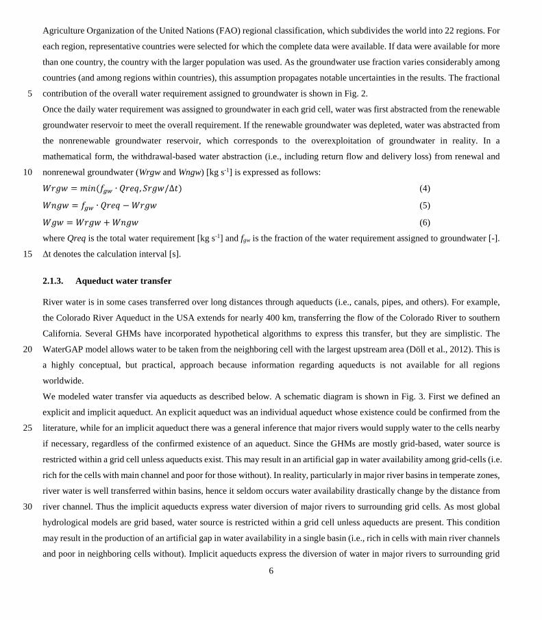
𝑊𝑊𝑄𝑄𝑊𝑊𝑊𝑊 = 𝑚𝑚𝑚𝑚𝑚𝑚 (𝑓𝑓𝑝𝑝𝑑𝑑 ∙ 𝑄𝑄𝑄𝑄𝑄𝑄𝑄𝑄, 𝑆𝑆𝑄𝑄𝑊𝑊𝑊𝑊/∆𝑄𝑄) (4)

𝑊𝑊𝑚𝑚𝑊𝑊𝑊𝑊 = 𝑓𝑓𝑝𝑝𝑑𝑑 ∙ 𝑄𝑄𝑄𝑄𝑄𝑄𝑄𝑄 −𝑊𝑊𝑄𝑄𝑊𝑊𝑊𝑊 (5)

𝑊𝑊𝑊𝑊𝑊𝑊 = 𝑊𝑊𝑄𝑄𝑊𝑊𝑊𝑊 + 𝑊𝑊𝑚𝑚𝑊𝑊𝑊𝑊 (6)

where Qreq is the total water requirement [kg s-1] and fgw is the fraction of the water requirement assigned to groundwater [-].

Δt denotes the calculation interval [s]. 15

2.1.3. Aqueduct water transfer

River water is in some cases transferred over long distances through aqueducts (i.e., canals, pipes, and others). For example,

the Colorado River Aqueduct in the USA extends for nearly 400 km, transferring the flow of the Colorado River to southern

California. Several GHMs have incorporated hypothetical algorithms to express this transfer, but they are simplistic. The

WaterGAP model allows water to be taken from the neighboring cell with the largest upstream area (Döll et al., 2012). This is 20

a highly conceptual, but practical, approach because information regarding aqueducts is not available for all regions

worldwide.

We modeled water transfer via aqueducts as described below. A schematic diagram is shown in Fig. 3. First we defined an

explicit and implicit aqueduct. An explicit aqueduct was an individual aqueduct whose existence could be confirmed from the

literature, while for an implicit aqueduct there was a general inference that major rivers would supply water to the cells nearby 25

if necessary, regardless of the confirmed existence of an aqueduct. Since the GHMs are mostly grid-based, water source is

restricted within a grid cell unless aqueducts exist. This may result in an artificial gap in water availability among grid-cells (i.e.

rich for the cells with main channel and poor for those without). In reality, particularly in major river basins in temperate zones,

river water is well transferred within basins, hence it seldom occurs water availability drastically change by the distance from

river channel. Thus the implicit aqueducts express water diversion of major rivers to surrounding grid cells. As most global 30

hydrological models are grid based, water source is restricted within a grid cell unless aqueducts are present. This condition

may result in the production of an artificial gap in water availability in a single basin (i.e., rich in cells with main river channels

and poor in neighboring cells without). Implicit aqueducts express the diversion of water in major rivers to surrounding grid

7

cells, reflecting our general observation that river water is well transferred within a basin, particularly in major river basins in

temperate zones. Hence, water availability seldom differs drastically with distance from main river channels.

For both types of aqueduct, global digital maps were prepared. For explicit aqueducts, the geographical locations of 55 major

aqueducts were identified. We collected publications relating to major aqueducts in six countries, namely, China, Egypt, India,

Israel, Pakistan, and the USA (listed in Table A2) and compiled them electronically on geographic information system (GIS) 5

software. We selected the aqueducts longer than 50 km or the length of the edge of a 0.5° × 0.5° grid cell. Then the origin (i.e.,

the point at which an aqueduct is diverted from the river), destination and route of each aqueduct were georeferenced on the

digital river network. The maps for the western USA, central China, the eastern Mediterranean region, and the Indian

Subcontinent are shown in Fig. 4. Because we set the base year at 2000, the south-north water transfer in China, which is

facilitated by one of the largest aqueducts in the world (completed in 2014) was not included in this map. 10

For implicit aqueducts, we considered that river water in a certain grid cell could be transferred to the neighboring cells if the

following conditions were met. First, the origin and destination were in the same basin (i.e., no inter-basin water transfer).

Second, the elevation of the destination had to be lower than the origin, which indicated that the gravity transfer of water was

possible. To determine this, we used global elevation data from ETOPO1 Global Relief (Amante and Eakins, 2009). We

up-scaled from the original resolution of 1’ × 1’ into 0.5° × 0.5° by extracting the minimum elevation. Third, the river 15

sequence of the destination had to be lower than that of the origin. The river sequence is a type of stream order assigned to

every grid cell (see the numbers on boxes in Fig. 3). It takes the value one at the cell of headwater, and subsequently the value

increases by one as the cell moves downstream. This condition was required to maintain the water balance of the river system,

because the calculation of river routing in H08 is conducted in the order of the river sequence. The river routing calculation at

the origin of aqueduct water transfer had to be conducted after the total volume of water transferred was fixed. 20

Because information regarding the capacity of aqueducts (i.e., the maximum rate of water transfer) was not available for most

cases, we assumed that water could be transferred unless the river flow at the origin was depleted. Due to limitations in data

availability, we assumed that both explicit and implicit aqueducts transfer water without any loss and delay. Hereafter, water

withdrawal via aqueducts is expressed as Waq in all mathematical expressions. Note that water withdrawal via aqueducts is

generally not distinguished from water withdrawal from a river in reality, and is seldom recorded independently. This point is 25

revisited in Section 3.1.3.

2.1.4. Local reservoirs

To represent flow regulation by the major dams in the global river network, several algorithms have been devised (Hanasaki et

al., 2006; Haddeland et al., 2006) and implemented in GHMs (Hanasaki et al., 2008b, Döll et al., 2009; Biemans et al., 2011).

How best to represent minor reservoirs located in tributaries remains to be determined. We defined the term global reservoirs to 30

be reservoirs located in the main channel of major rivers, which were explicitly delineated by the digital global river map used

in the GHM, and defined local reservoirs as those located in the tributaries. A straightforward approach is to add the storage

capacity of local reservoirs to that of global reservoirs (e.g., Wada et al., 2014), but this may overestimate the regulated flow

8

capacity. Some studies have treated global and local reservoirs differently. The original H08 assumed that all reservoirs with

less than 1 km3 of storage capacity were local reservoirs (Hanasaki et al., 2010; they referred to them as “medium-size

reservoirs”). Because the geographical information regarding local reservoirs was not available at that time, the authors

spatially distributed the national total capacity of local reservoirs weighted by the population distribution. They assumed that

local reservoirs were not regulating river flows, but acted as an ideal water storage location within grid cells. All the runoff 5

generated in a grid cell runs into storage and the stored water can be used at any time. Wisser et al. (2010) introduced a

similar algorithm for local reservoirs (they referred to them as "small reservoirs") into WBMplus (note that the abstraction

from “small reservoirs” becomes unrealistically large, as much as 989 km3yr-1 in their formulations, i.e., one third of the total

global water withdrawal).

We modified the original H08 algorithms for global and local reservoir operation (i.e., Hanasaki et al., 2006; 2010) as below. A 10

schematic diagram of global and local reservoirs is shown in Fig. 1.

First, the GRanD global inventory of reservoirs (Lehner et al., 2011) was used to identify the location of global and local

reservoirs. Global and local reservoirs were distinguished by their catchment area. GRanD includes the specifications of 6852

reservoirs with a storage capacity larger than 0.1 km3, and all of them are georeferenced on the digital river network of

HydroSHEDS (Lehner et al., 2008) at a spatial resolution of 15 arc-second. This enabled us to estimate the catchment area of 15

all the reservoirs, which has seldom been performed in previous global inventories of large dams. We set the threshold of 5000

km2 (equivalent to the area of approximately two 0.5° × 0.5° grid cells) to separate global and local reservoirs. Note that the

shape of the watershed and channel was not well reproduced in the digital river map of 0.5° × 0.5° for basins less than 5000

km2. This resulted in 963 reservoirs with 4773 km3 of total storage capacity being categorized as global reservoirs, and the

remaining 5824 reservoirs (1300 km3) being categorized as local reservoirs. In cases where multiple reservoirs were assigned 20

to one cell, their capacity was aggregated in each grid cell. The catchment area of a local reservoir was equal to that of the

largest within a grid cell, unless the area did not exceed the area of the grid cell.

Runoff generated within the catchment area of a local reservoir flows into storage. When the storage exceeds its storage

capacity, the excess water flows into a river (Fig. 1). The storage in a local reservoir acts as an ideal tank, with water loss due to

surface evaporation and other factors ignored. A local reservoir is accessible from the grid cells where it is located. It is also 25

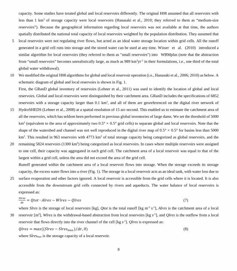
accessible from the downstream grid cells connected by rivers and aqueducts. The water balance of local reservoirs is

expressed as: 𝑑𝑑𝑆𝑆𝑟𝑟𝑆𝑆𝑆𝑆𝑑𝑑𝑡𝑡

= 𝑄𝑄𝑄𝑄𝑄𝑄𝑄𝑄 ∙ 𝐴𝐴𝐴𝐴𝑄𝑄𝑄𝑄𝐴𝐴 −𝑊𝑊𝐴𝐴𝑄𝑄𝑄𝑄𝐴𝐴 − 𝑄𝑄𝐴𝐴𝑄𝑄𝑄𝑄𝐴𝐴 (7)

where Slres is the storage of local reservoirs [kg], Qtot is the total runoff [kg m-2 s-1], Alres is the catchment area of a local

reservoir [m2], Wlres is the withdrawal-based abstraction from local reservoirs [kg s-1], and Qlres is the outflow from a local 30

reservoir that flows directly into the river channel of the cell [kg s-1]. Qlres is expressed as:

𝑄𝑄𝐴𝐴𝑄𝑄𝑄𝑄𝐴𝐴 = 𝑚𝑚𝑚𝑚𝑚𝑚 ((𝑆𝑆𝐴𝐴𝑄𝑄𝑄𝑄𝐴𝐴 − 𝑆𝑆𝐴𝐴𝑄𝑄𝑄𝑄𝐴𝐴𝑚𝑚𝑚𝑚𝑚𝑚) 𝛥𝛥𝑄𝑄⁄ , 0) (8)

where Slresmax is the storage capacity of a local reservoir.

9

2.1.5. Seawater desalination

Seawater desalination is a practical method to obtain freshwater in arid coastal regions. It currently accounts for approximately

0.1% of the total water withdrawal in the world, but production is rapidly increasing in arid regions (www.desaldata.com).

Desalination was not incorporated in most of GHMs until recently. Oki et al. (2001) included the reported values of desalinated

water production in total freshwater resources in a nation-based water scarcity assessment. Wada et al. (2011) spatially 5

distributed the reported national volume of desalinated water produced along the coastline and assumed it was an available

freshwater resource in the PCR-GLOBWB model. Recently, Hanasaki et al. (2016) developed a stand-alone model to estimate

the geographical extent of areas where desalinated seawater is used and the volume of production.

We incorporated the seawater desalination scheme of Hanasaki et al. (2016) into H08. Their seawater desalination scheme

consists of two parts. The first estimates the geographical extent of the area utilizing seawater desalination (AUSD), where 10

seawater desalination is likely to be the dominant local water source. The second estimates the volume of water production.

Hanasaki et al. (2016) found that the AUSD can be defined as all grid cells meeting all of three conditions, namely, the nations

whose gross domestic product (GDP) exceeds 14,000 USD person-1 yr-1 in terms of purchasing power parity (PPP), the

humidity index (precipitation over potential evapotranspiration) falls below 8%, and the cells are located within three

consecutive 0.5° × 0.5° grid cells (approximately 165 km along the equator) of seashore. By assuming seawater desalination is 15

not used for irrigation, and all of the municipal and industrial water withdrawal in AUSD cells is abstracted by seawater

desalination, which is supported by the available statistical records in Hanasaki et al. (2016), we could estimate the quantitative

spatiotemporal distribution of withdrawal from seawater desalination. Hereafter, water withdrawal of seawater desalination is

expressed as Wdes in mathematical expressions.

2.1.6. Return flow and delivery loss 20

Return flow and delivery (conveyance) loss are important processes in water abstraction. Döll and Siebert (2002) reported that

of the 2549 km3yr-1 of global total water withdrawn for irrigation, 1092 km3yr-1 is used for consumption (evapotranspiration),

which indicates that nearly 60% of water withdrawn for irrigation becomes return flow and delivery loss. We defined return

flow as the flow of water that is withdrawn from sources, but is not consumed and is discharged into the original or some other

water body. Delivery loss is the flow of water that is evaporated during delivery. LPJmL includes the return flow and delivery 25

loss of irrigation (Rost et al., 2008). In their model, a certain fraction of abstracted water is delivered to cropland, which is

determined by the regional irrigation efficiency. The authors then assumed that 50% of the undelivered water returns to the

river channel, and the remaining 50% is lost due to evaporation.

To represent return flow and delivery loss for surface water abstraction, the algorithm of Rost et al. (2008) was adopted. Water

abstraction is expressed as follows: 30

𝑊𝑊 = 𝐶𝐶 + 𝐿𝐿 + 𝑅𝑅 (9)

𝐶𝐶 = 𝑄𝑄𝑊𝑊 (10)

10

𝐿𝐿 = 𝐴𝐴 (1 − 𝑄𝑄)𝑊𝑊 (11)

𝑅𝑅 = (1 − 𝐴𝐴)(1 − 𝑄𝑄)𝑊𝑊 (12)

where W is withdrawal-based water abstraction taken from various sources [kg s-1], C is the consumptive water use, or the

volume of water evaporated or transpired at the destination [kg s-1]. L is the delivery loss or the volume of water evaporated

during delivery [kg s-1], R is the return flow (drainage) to the river stream [kg s-1], e is the ratio of consumption to withdrawal 5

[-], and l is the proportion lost during delivery [-]. W, C, L, e, and l are all sector and water-source specific. Return flow was

drained into the subsequent downstream grid cell in the next time step (i.e. next day in a standard model set up).

The coefficient e for each sector was determined as follows. For surface water irrigation, the irrigation efficiency rate provided

by Döll and Siebert (2002) was used. For groundwater irrigation, the rate was set at unity globally; we assumed that the

irrigation wells are all located near to where the water was used. This does not necessarily mean that the abstracted 10

groundwater was all consumed by evapotranspiration. As described in Appendix A, in H08, irrigation water is added to the soil

moisture of the irrigated portion of a grid cell. A substantial portion of it eventually turns into subsurface runoff and

groundwater recharge, which is not used for evapotranspiration by plants. For industrial and municipal water, this proportion

was set at 0.1 and 0.15 based on work by Shikilomanov (2000) for both surface and groundwater. To the best of our knowledge,

there is no systematic global inventory of the amount lost during delivery (l). Following Rost et al. (2008), for surface water 15

irrigation, we assumed the proportion lost was 0.5 globally. For groundwater irrigation, we assumed there was zero loss

globally because we assumed the distance of delivery to be negligible. Industrial and municipal water is drained underground;

hence, we also assumed the loss to be zero globally, because water is seldom lost by evaporation, at least in the urbanized areas

where the majority of industrial and municipal water is used.

2.1.7. Surface water balance 20

Surface water abstraction is represented as follows. To fulfill the surface water requirement, water is first taken from local river

flow, which is regulated by a global reservoir. If the river is depleted and the surface water requirement is not fulfilled, water

was taken from the river flow at the origin of an aqueduct. If the surface water requirement is still not met, water is taken from

a local reservoir in the same cell or from an upstream location. If the grid cells in question are categorized as the AUSD (see

Section 2.1.5), the surface water requirement for industrial and municipal water is taken from seawater desalination, and 25

neither river flow nor local reservoirs are used. If the surface water requirement is still not met, the remaining volume is classed

as the surface water deficit or the volume of water that is unable to be abstracted from available surface water sources.

Water was abstracted by sector in the order of municipality, industry, and irrigation. The order of water withdrawal reflects the

distinct differences in water use intensity on the general premise that priority should be given to high value-added products in

resources allocation. Municipal, industrial, and agricultural water use intensities per value added (service, manufacturing and 30

power generation, and agricultural sectors) are estimated at 0.012, 0.063, and 2.2 106m3 106USD-1, respectively.

The H08 model provides two modes of surface water deficit. Option 1 is to secure the fulfillment of the water requirement by

assuming an imaginary unlimited surface water source and taking water from it as necessary. This is referred to as water

11

abstraction from unspecified surface water (USW). A precondition of this study was that water withdrawal estimates were

based on values reported in the AQUASTAT database. As shown in Section 2.2.1 and Appendix A, municipal and industrial

water requirements were taken from the database, and simulated irrigation water ws also carefully compared with these data

(Supplemental Text S1). Here we presumed that AQUASTAT reported the volume of water that was actually abstracted in

each nation. Option 1 strictly followed this condition and compensated with unspecified surface water in case where surface 5

water data were not available. Option 2 is to abandon the fulfilment of the water requirement and leave the remaining volume

as a deficit. In other words, option 1 places more reliance on the estimated water requirement, which is largely statistically

based (i.e., the national annual water withdrawal volume for municipal and industrial use was derived from the AQUASTAT

database; Appendix A) or well validated (i.e., the national annual simulated irrigation water withdrawal volume agrees well

with AQUASTAT data; Appendix A, Figure S2). It is difficult to explain where USW comes from, which is a key shortcoming 10

of this option. Note that adding water from imaginary source to the H08 is nearly the only way to quantitatively estimate the

volume of missing source water, particularly for irrigation. As shown in Appendix A, the irrigation water requirement was

determined by the soil moisture deficit which shows highly nonlinear behavior and interacts with other components. An

imaginary source of water fills the deficit at every calculation interval, such that the accumulation of water equals the volume

of missing source water. In contrast, option 2 places less reliance on the estimated water requirement. In this study, we used 15

option 1. The estimated volume of abstraction from USW should be interpreted with care, and further consideration is given in

Section 3.4.

The incorporation and coupling of all the schemes enabled H08 to express water abstraction as follows:

𝑊𝑊𝑄𝑄𝑄𝑄𝑄𝑄 = 𝑊𝑊𝑊𝑊𝑊𝑊 + 𝑊𝑊𝐴𝐴𝑄𝑄𝑓𝑓 (13)

where Wtot and Wsrf are total and surface water withdrawal, respectively [kg s-1]. Wsrf is expressed as, 20

𝑊𝑊𝐴𝐴𝑄𝑄𝑓𝑓 = 𝑊𝑊𝑄𝑄𝑚𝑚𝑊𝑊 + 𝑊𝑊𝑚𝑚𝑄𝑄 + 𝑊𝑊𝐴𝐴𝑄𝑄𝑄𝑄𝐴𝐴 + 𝑊𝑊𝑊𝑊𝑄𝑄𝐴𝐴 + 𝑊𝑊𝑊𝑊𝐴𝐴𝑊𝑊 (14)

where Wriv and Wusw are the withdrawal-based abstraction from a river and USW [kg s-1], respectively. When Option 1 is

taken, the following relationship is established:

𝑊𝑊𝐴𝐴𝑄𝑄𝑓𝑓 = �1 − 𝑓𝑓𝑝𝑝𝑑𝑑�×𝑄𝑄𝑄𝑄𝑄𝑄𝑄𝑄 (15)

2.2. Data 25

2.2.1. Geographical data

Various geographical maps were used to set the boundary condition of the sub-models of H08, as shown in Table 1. We used

the same setting as Hanasaki et al. (2013b) in this study. The geographical data used covered the whole globe, except

Antarctica, at a spatial resolution of 0.5° × 0.5° for the year 2000. Temporal variations in geographical conditions were not

considered in this study due to lack of reliable and consistent information. 30

The geographical data directly relevant to the key results are described here. The irrigation water requirement was substantially

influenced by the irrigated area (Siebert et al., 2010), crop type (Monfreda et al., 2010), crop intensity, and irrigation efficiency

12

(Döll and Siebert, 2002). The industrial and municipal water requirement was determined by national estimates for the year

2000 provided by AQUASTAT (www.fao.org/nr/aquastat/). The national estimates were spatially interpolated and weighted

by the population distribution of the Center for International Earth Science Information Network (CIESIN) and Columbia

University and Centro Internacional de Agricultura Tropical (CIAT) (2005).

2.2.2. Meteorological data 5

To run H08, a global meteorological dataset is required. We used the WATCH forcing data methodology applied to European

Centre for Medium-Range Weather Forecasts (ECMWF) re-analysis (ERA)-Interim data (hereafter WFDEI, Weedon et al.,

2014) in this study. The WATCH forcing methodology represents sub-daily reanalysis data scaled arithmetically to make the

mean values and the range of variation consistent with spatio-temporary coarse ground observation data. WFDEI contain eight

meteorological variables, namely, air temperature, specific humidity, wind speed, surface air pressure, longwave and 10

shortwave downward radiation, rainfall, and snowfall. All variables are indispensable in the H08 model to solve the land

surface water and energy balance. WFDEI covers the whole globe at a spatial resolution of 0.5° × 0.5°, and the period of

1979-2013 at a daily interval.

2.3. Simulations

Simulations were conducted for 35 years from 1979 to 2013 using WFDEI. The simulations for the last 30 years were used for 15

analyses (1984-2013), with the first five years used only as a spin-up. The geographical data were fixed at the year 2000 due to

the limited availability of temporal variations. The calculation interval was a day. This means that all the water flows

accompanying both natural and human processes were calculated and exchanged among components at a daily interval, strictly

tracking all water fluxes and storage; therefore, no unexplained water imbalance.

As mentioned above, the original H08 consists of six sub-models (land surface hydrology, river routing, reservoir operation, 20

water abstraction, crop growth, and environmental flow requirement). We developed six new schemes. Two simulations with

different combinations of sub-models and schemes were conducted in this study. The first was a naturalized simulation, which

disabled all of the sub-models of human activity (NAT). For this simulation, only the land surface hydrology sub-model

enhanced by the groundwater recharge scheme and the river routing sub-models were used. The second was a simulation that

enabled all sub-models of human activities to be enhanced by the abovementioned six schemes (ALL). For this simulation, the 25

daily grid-based water requirement was fulfilled by any one of the six explicit water sources (i.e., renewable groundwater,

nonrenewable groundwater, river, aqueduct water transfer, local reservoirs, seawater desalination) or USW. In addition, two

auxiliary simulations were conducted. One is the simulation to reproduce the behavior of the original H08 (the ORIG

simulation) which is described in Supplemental Text S4. The other is the simulation to allow additional abstraction from the

renewable groundwater reservoir in case unspecified surface water is used (the SWT simulation) which is described in 30

Supplemental Text S5.

13

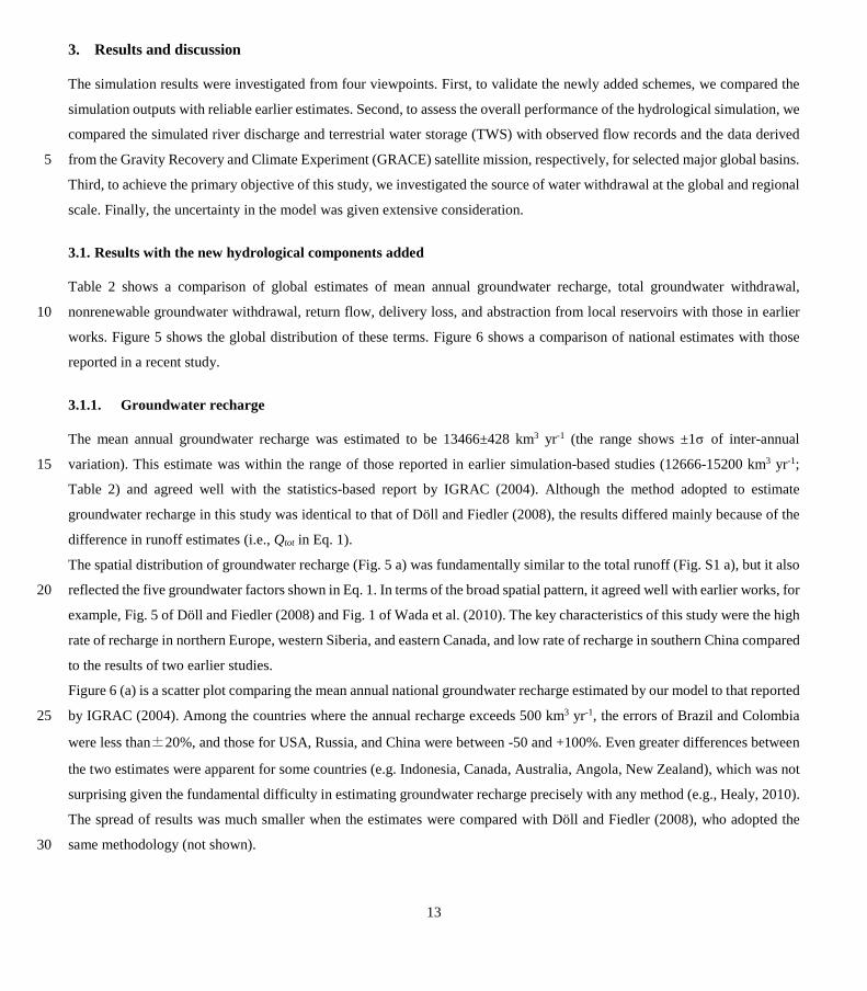
3. Results and discussion

The simulation results were investigated from four viewpoints. First, to validate the newly added schemes, we compared the

simulation outputs with reliable earlier estimates. Second, to assess the overall performance of the hydrological simulation, we

compared the simulated river discharge and terrestrial water storage (TWS) with observed flow records and the data derived

from the Gravity Recovery and Climate Experiment (GRACE) satellite mission, respectively, for selected major global basins. 5

Third, to achieve the primary objective of this study, we investigated the source of water withdrawal at the global and regional

scale. Finally, the uncertainty in the model was given extensive consideration.

3.1. Results with the new hydrological components added

Table 2 shows a comparison of global estimates of mean annual groundwater recharge, total groundwater withdrawal,

nonrenewable groundwater withdrawal, return flow, delivery loss, and abstraction from local reservoirs with those in earlier 10

works. Figure 5 shows the global distribution of these terms. Figure 6 shows a comparison of national estimates with those

reported in a recent study.

3.1.1. Groundwater recharge

The mean annual groundwater recharge was estimated to be 13466±428 km3 yr-1 (the range shows ±1σ of inter-annual

variation). This estimate was within the range of those reported in earlier simulation-based studies (12666-15200 km3 yr-1; 15

Table 2) and agreed well with the statistics-based report by IGRAC (2004). Although the method adopted to estimate

groundwater recharge in this study was identical to that of Döll and Fiedler (2008), the results differed mainly because of the

difference in runoff estimates (i.e., Qtot in Eq. 1).

The spatial distribution of groundwater recharge (Fig. 5 a) was fundamentally similar to the total runoff (Fig. S1 a), but it also

reflected the five groundwater factors shown in Eq. 1. In terms of the broad spatial pattern, it agreed well with earlier works, for 20

example, Fig. 5 of Döll and Fiedler (2008) and Fig. 1 of Wada et al. (2010). The key characteristics of this study were the high

rate of recharge in northern Europe, western Siberia, and eastern Canada, and low rate of recharge in southern China compared

to the results of two earlier studies.

Figure 6 (a) is a scatter plot comparing the mean annual national groundwater recharge estimated by our model to that reported

by IGRAC (2004). Among the countries where the annual recharge exceeds 500 km3 yr-1, the errors of Brazil and Colombia 25

were less than±20%, and those for USA, Russia, and China were between -50 and +100%. Even greater differences between

the two estimates were apparent for some countries (e.g. Indonesia, Canada, Australia, Angola, New Zealand), which was not

surprising given the fundamental difficulty in estimating groundwater recharge precisely with any method (e.g., Healy, 2010).

The spread of results was much smaller when the estimates were compared with Döll and Fiedler (2008), who adopted the

same methodology (not shown). 30

14

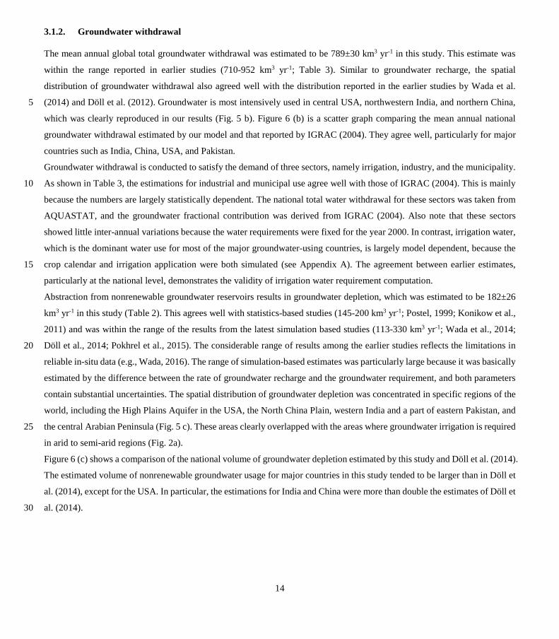
3.1.2. Groundwater withdrawal

The mean annual global total groundwater withdrawal was estimated to be 789±30 km3 yr-1 in this study. This estimate was

within the range reported in earlier studies (710-952 km3 yr-1; Table 3). Similar to groundwater recharge, the spatial

distribution of groundwater withdrawal also agreed well with the distribution reported in the earlier studies by Wada et al.

(2014) and Döll et al. (2012). Groundwater is most intensively used in central USA, northwestern India, and northern China, 5

which was clearly reproduced in our results (Fig. 5 b). Figure 6 (b) is a scatter graph comparing the mean annual national

groundwater withdrawal estimated by our model and that reported by IGRAC (2004). They agree well, particularly for major

countries such as India, China, USA, and Pakistan.

Groundwater withdrawal is conducted to satisfy the demand of three sectors, namely irrigation, industry, and the municipality.

As shown in Table 3, the estimations for industrial and municipal use agree well with those of IGRAC (2004). This is mainly 10

because the numbers are largely statistically dependent. The national total water withdrawal for these sectors was taken from

AQUASTAT, and the groundwater fractional contribution was derived from IGRAC (2004). Also note that these sectors

showed little inter-annual variations because the water requirements were fixed for the year 2000. In contrast, irrigation water,

which is the dominant water use for most of the major groundwater-using countries, is largely model dependent, because the

crop calendar and irrigation application were both simulated (see Appendix A). The agreement between earlier estimates, 15

particularly at the national level, demonstrates the validity of irrigation water requirement computation.

Abstraction from nonrenewable groundwater reservoirs results in groundwater depletion, which was estimated to be 182±26

km3 yr-1 in this study (Table 2). This agrees well with statistics-based studies (145-200 km3 yr-1; Postel, 1999; Konikow et al.,

2011) and was within the range of the results from the latest simulation based studies (113-330 km3 yr-1; Wada et al., 2014;

Döll et al., 2014; Pokhrel et al., 2015). The considerable range of results among the earlier studies reflects the limitations in 20

reliable in-situ data (e.g., Wada, 2016). The range of simulation-based estimates was particularly large because it was basically

estimated by the difference between the rate of groundwater recharge and the groundwater requirement, and both parameters

contain substantial uncertainties. The spatial distribution of groundwater depletion was concentrated in specific regions of the

world, including the High Plains Aquifer in the USA, the North China Plain, western India and a part of eastern Pakistan, and

the central Arabian Peninsula (Fig. 5 c). These areas clearly overlapped with the areas where groundwater irrigation is required 25

in arid to semi-arid regions (Fig. 2a).

Figure 6 (c) shows a comparison of the national volume of groundwater depletion estimated by this study and Döll et al. (2014).

The estimated volume of nonrenewable groundwater usage for major countries in this study tended to be larger than in Döll et

al. (2014), except for the USA. In particular, the estimations for India and China were more than double the estimates of Döll et

al. (2014). 30

15

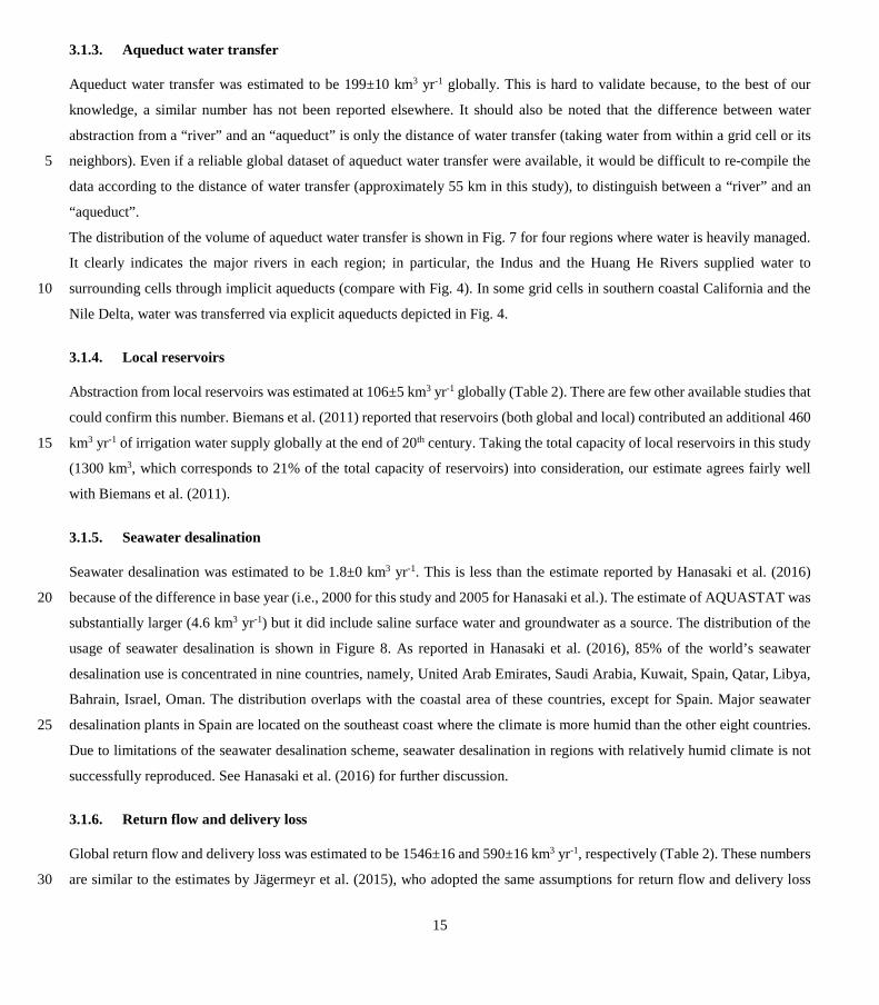
3.1.3. Aqueduct water transfer

Aqueduct water transfer was estimated to be 199±10 km3 yr-1 globally. This is hard to validate because, to the best of our

knowledge, a similar number has not been reported elsewhere. It should also be noted that the difference between water

abstraction from a “river” and an “aqueduct” is only the distance of water transfer (taking water from within a grid cell or its

neighbors). Even if a reliable global dataset of aqueduct water transfer were available, it would be difficult to re-compile the 5

data according to the distance of water transfer (approximately 55 km in this study), to distinguish between a “river” and an

“aqueduct”.

The distribution of the volume of aqueduct water transfer is shown in Fig. 7 for four regions where water is heavily managed.

It clearly indicates the major rivers in each region; in particular, the Indus and the Huang He Rivers supplied water to

surrounding cells through implicit aqueducts (compare with Fig. 4). In some grid cells in southern coastal California and the 10

Nile Delta, water was transferred via explicit aqueducts depicted in Fig. 4.

3.1.4. Local reservoirs

Abstraction from local reservoirs was estimated at 106±5 km3 yr-1 globally (Table 2). There are few other available studies that

could confirm this number. Biemans et al. (2011) reported that reservoirs (both global and local) contributed an additional 460

km3 yr-1 of irrigation water supply globally at the end of 20th century. Taking the total capacity of local reservoirs in this study 15

(1300 km3, which corresponds to 21% of the total capacity of reservoirs) into consideration, our estimate agrees fairly well

with Biemans et al. (2011).

3.1.5. Seawater desalination

Seawater desalination was estimated to be 1.8±0 km3 yr-1. This is less than the estimate reported by Hanasaki et al. (2016)

because of the difference in base year (i.e., 2000 for this study and 2005 for Hanasaki et al.). The estimate of AQUASTAT was 20

substantially larger (4.6 km3 yr-1) but it did include saline surface water and groundwater as a source. The distribution of the

usage of seawater desalination is shown in Figure 8. As reported in Hanasaki et al. (2016), 85% of the world’s seawater

desalination use is concentrated in nine countries, namely, United Arab Emirates, Saudi Arabia, Kuwait, Spain, Qatar, Libya,

Bahrain, Israel, Oman. The distribution overlaps with the coastal area of these countries, except for Spain. Major seawater

desalination plants in Spain are located on the southeast coast where the climate is more humid than the other eight countries. 25

Due to limitations of the seawater desalination scheme, seawater desalination in regions with relatively humid climate is not

successfully reproduced. See Hanasaki et al. (2016) for further discussion.

3.1.6. Return flow and delivery loss

Global return flow and delivery loss was estimated to be 1546±16 and 590±16 km3 yr-1, respectively (Table 2). These numbers

are similar to the estimates by Jägermeyr et al. (2015), who adopted the same assumptions for return flow and delivery loss 30

16

(Rost et al., 2008). Both return flow and delivery loss were spatially concentrated in Asia, where surface irrigation is

predominant (Figs. 5 d-e and 2 a). This primarily reflects the practice of paddy irrigation, which requires large amounts of

irrigation water to flood the paddy field, with an accompanying low irrigation efficiency.

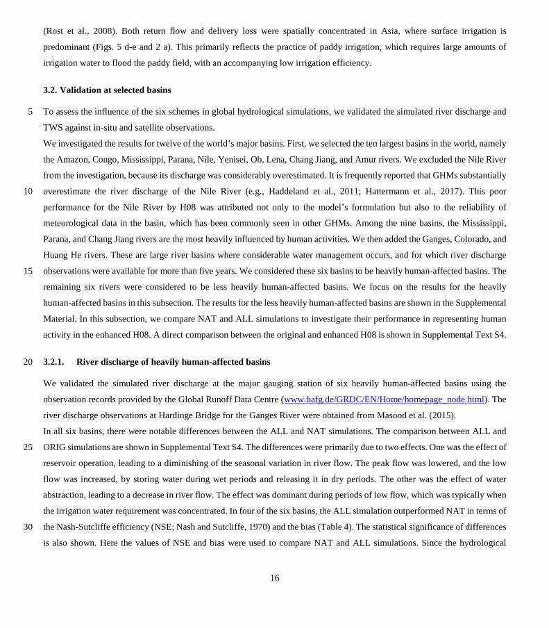
3.2. Validation at selected basins

To assess the influence of the six schemes in global hydrological simulations, we validated the simulated river discharge and 5

TWS against in-situ and satellite observations.

We investigated the results for twelve of the world’s major basins. First, we selected the ten largest basins in the world, namely

the Amazon, Congo, Mississippi, Parana, Nile, Yenisei, Ob, Lena, Chang Jiang, and Amur rivers. We excluded the Nile River

from the investigation, because its discharge was considerably overestimated. It is frequently reported that GHMs substantially

overestimate the river discharge of the Nile River (e.g., Haddeland et al., 2011; Hattermann et al., 2017). This poor 10

performance for the Nile River by H08 was attributed not only to the model’s formulation but also to the reliability of

meteorological data in the basin, which has been commonly seen in other GHMs. Among the nine basins, the Mississippi,

Parana, and Chang Jiang rivers are the most heavily influenced by human activities. We then added the Ganges, Colorado, and

Huang He rivers. These are large river basins where considerable water management occurs, and for which river discharge

observations were available for more than five years. We considered these six basins to be heavily human-affected basins. The 15

remaining six rivers were considered to be less heavily human-affected basins. We focus on the results for the heavily

human-affected basins in this subsection. The results for the less heavily human-affected basins are shown in the Supplemental

Material. In this subsection, we compare NAT and ALL simulations to investigate their performance in representing human

activity in the enhanced H08. A direct comparison between the original and enhanced H08 is shown in Supplemental Text S4.

3.2.1. River discharge of heavily human-affected basins 20

We validated the simulated river discharge at the major gauging station of six heavily human-affected basins using the

observation records provided by the Global Runoff Data Centre (www.bafg.de/GRDC/EN/Home/homepage_node.html). The

river discharge observations at Hardinge Bridge for the Ganges River were obtained from Masood et al. (2015).

In all six basins, there were notable differences between the ALL and NAT simulations. The comparison between ALL and

ORIG simulations are shown in Supplemental Text S4. The differences were primarily due to two effects. One was the effect of 25

reservoir operation, leading to a diminishing of the seasonal variation in river flow. The peak flow was lowered, and the low

flow was increased, by storing water during wet periods and releasing it in dry periods. The other was the effect of water

abstraction, leading to a decrease in river flow. The effect was dominant during periods of low flow, which was typically when

the irrigation water requirement was concentrated. In four of the six basins, the ALL simulation outperformed NAT in terms of

the Nash-Sutcliffe efficiency (NSE; Nash and Sutcliffe, 1970) and the bias (Table 4). The statistical significance of differences 30

is also shown. Here the values of NSE and bias were used to compare NAT and ALL simulations. Since the hydrological

17

parameters of H08 were not tuned at individual basins, the results of NSE and bias in some basins were not as high as those of

calibrated models (see Hattermann et al. 2017 for comprehensive discussion).

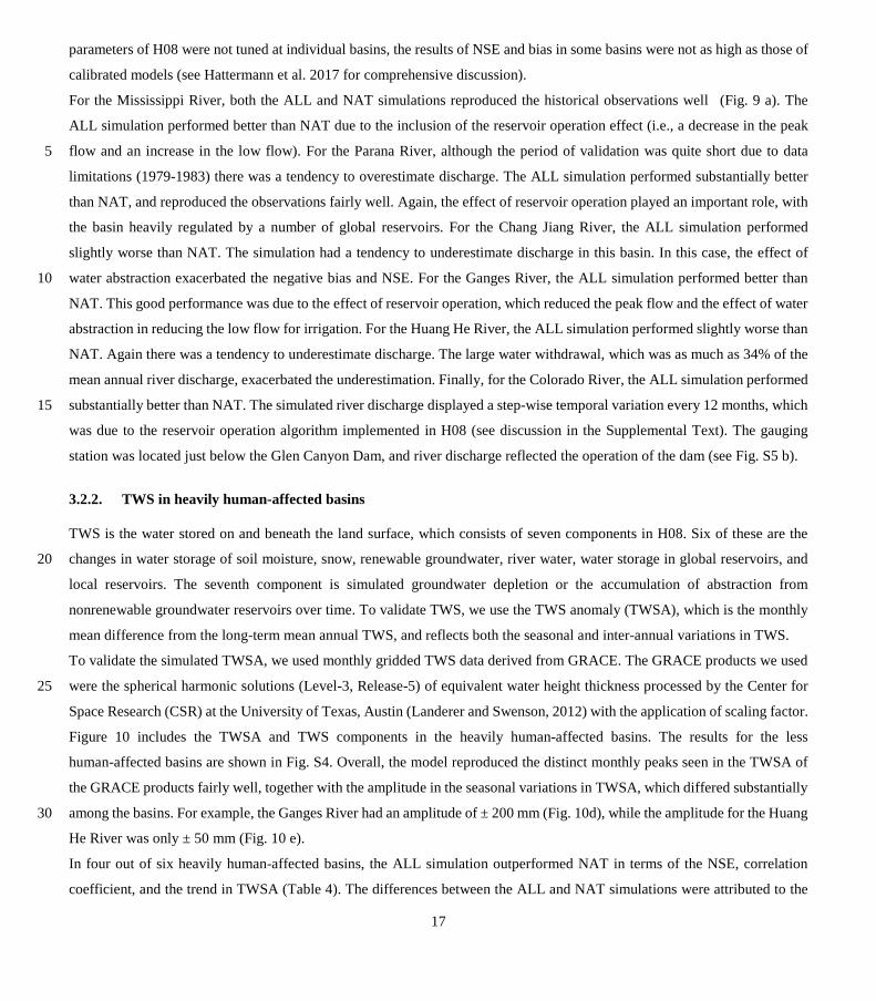
For the Mississippi River, both the ALL and NAT simulations reproduced the historical observations well (Fig. 9 a). The

ALL simulation performed better than NAT due to the inclusion of the reservoir operation effect (i.e., a decrease in the peak

flow and an increase in the low flow). For the Parana River, although the period of validation was quite short due to data 5

limitations (1979-1983) there was a tendency to overestimate discharge. The ALL simulation performed substantially better

than NAT, and reproduced the observations fairly well. Again, the effect of reservoir operation played an important role, with

the basin heavily regulated by a number of global reservoirs. For the Chang Jiang River, the ALL simulation performed

slightly worse than NAT. The simulation had a tendency to underestimate discharge in this basin. In this case, the effect of

water abstraction exacerbated the negative bias and NSE. For the Ganges River, the ALL simulation performed better than 10

NAT. This good performance was due to the effect of reservoir operation, which reduced the peak flow and the effect of water

abstraction in reducing the low flow for irrigation. For the Huang He River, the ALL simulation performed slightly worse than

NAT. Again there was a tendency to underestimate discharge. The large water withdrawal, which was as much as 34% of the

mean annual river discharge, exacerbated the underestimation. Finally, for the Colorado River, the ALL simulation performed

substantially better than NAT. The simulated river discharge displayed a step-wise temporal variation every 12 months, which 15

was due to the reservoir operation algorithm implemented in H08 (see discussion in the Supplemental Text). The gauging

station was located just below the Glen Canyon Dam, and river discharge reflected the operation of the dam (see Fig. S5 b).

3.2.2. TWS in heavily human-affected basins

TWS is the water stored on and beneath the land surface, which consists of seven components in H08. Six of these are the

changes in water storage of soil moisture, snow, renewable groundwater, river water, water storage in global reservoirs, and 20

local reservoirs. The seventh component is simulated groundwater depletion or the accumulation of abstraction from

nonrenewable groundwater reservoirs over time. To validate TWS, we use the TWS anomaly (TWSA), which is the monthly

mean difference from the long-term mean annual TWS, and reflects both the seasonal and inter-annual variations in TWS.

To validate the simulated TWSA, we used monthly gridded TWS data derived from GRACE. The GRACE products we used

were the spherical harmonic solutions (Level-3, Release-5) of equivalent water height thickness processed by the Center for 25

Space Research (CSR) at the University of Texas, Austin (Landerer and Swenson, 2012) with the application of scaling factor.

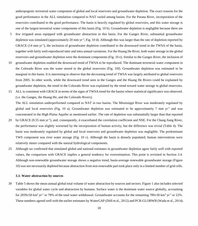
Figure 10 includes the TWSA and TWS components in the heavily human-affected basins. The results for the less

human-affected basins are shown in Fig. S4. Overall, the model reproduced the distinct monthly peaks seen in the TWSA of

the GRACE products fairly well, together with the amplitude in the seasonal variations in TWSA, which differed substantially

among the basins. For example, the Ganges River had an amplitude of ± 200 mm (Fig. 10d), while the amplitude for the Huang 30

He River was only ± 50 mm (Fig. 10 e).

In four out of six heavily human-affected basins, the ALL simulation outperformed NAT in terms of the NSE, correlation

coefficient, and the trend in TWSA (Table 4). The differences between the ALL and NAT simulations were attributed to the

18

anthropogenic terrestrial water component of global and local reservoirs and groundwater depletion. The exact reasons for the

good performance in the ALL simulation compared to NAT varied among basins. For the Parana River, incorporation of the

reservoirs contributed to the good performance. The basin is heavily regulated by global reservoirs, and this water storage is

one of the largest terrestrial water components of this basin (Fig. 10 b). Groundwater depletion is negligible because there are

few irrigated areas equipped with groundwater abstraction in this basin. For the Ganges River, substantial groundwater 5

depletion was simulated (approximately 20 mm yr-1; Fig. 10 d). Although this was larger than the rate of depletion reported by

GRACE (14 mm yr-1), the inclusion of groundwater depletion contributed to the downward trend in the TWSA of the basin,

together with fairly well-reproduced inter and intra annual variations. For the Huang He River, both water storage in the global

reservoirs and groundwater depletion were the dominant components (Fig. 10 e). Similar to the Ganges River, the inclusion of

groundwater depletion enabled the downward trend of TWSA to be reproduced. The dominant terrestrial water component in 10

the Colorado River was the water stored in the global reservoirs (Fig. 10f). Groundwater depletion was estimated to be

marginal in this basin. It is interesting to observe that the decreasing trend of TWSA was largely attributed to global reservoirs

from 2005. In other words, while the downward trend seen in the Ganges and the Huang He Rivers could be explained by

groundwater depletion, the trend in the Colorado River was explained by the trend toward water storage in global reservoirs.

ALL is consistent with GRACE in terms of the signs of TWSA trend for the basins where statistical significance was observed. 15

(i.e. the Ganges, the Huang He, and the Colorado Rivers).

The ALL simulation underperformed compared to NAT in two basins. The Mississippi River was moderately regulated by

global and local reservoirs (Fig. 10 a). Groundwater depletion was estimated to be approximately 7 mm yr-1 and was

concentrated in the High Plains Aquifer as mentioned earlier. The rate of depletion was substantially larger than that reported

by GRACE (0.55 mm yr-1), and, consequently, it exacerbated the correlation coefficient and NSE. For the Chang Jiang River, 20

the performance was slightly worsened by the incorporation of human activity, but the difference was trivial (Table 4). The

basin was moderately regulated by global and local reservoirs and groundwater depletion was negligible. The predominant

TWS component was river water storage (Fig. 10 c). Although the basin is densely populated, human interventions were

relatively minor compared with the natural hydrological components.

Although we confirmed that simulated global and national estimates in groundwater depletion agree fairly well with reported 25

values, the comparison with GRACE implies a general tendency for overestimation. This point is revisited in Section 3.4.

Although non-renewable groundwater storage shows a negative trend, basin-average renewable groundwater storage (Figure

10) was not necessarily depleted because abstraction from non-renewable part took place only in a limited number of grid cells.

3.3. Water abstraction by sources

Table 5 shows the mean annual global total volume of water abstraction by sources and sectors. Figure 1 also includes selected 30

variables for global water cycle and abstraction by humans. Surface water is the dominant water source globally, accounting

for 2839±50 km3 yr-1 or 78% of the total water withdrawal. Groundwater accounts for the remaining 789±30 km3 yr-1 or 22%.

These numbers agreed well with the earlier estimates by WaterGAP (Döll et al., 2012) and PCR-GLOBWB (Wada et al., 2014).

19

Total, surface, and groundwater water withdrawal were very close to the values obtained from AQUASTAT and IGRAC

(2004).

The enhanced H08 enabled us to break down these estimates further in terms of water sources and sectors. For irrigation water,

more than half of the surface water consumed comes from rivers. Aqueducts and local reservoirs also make important

contributions (9 and 5%, respectively). No seawater desalination was used because it was assumed it was not used for irrigation. 5

USW (see Section 2.1.7) was very large in the irrigation sector. It accounted for 33% of the annual total agricultural water

withdrawal. This large volume of USW is discussed in Section 3.4.1. As for groundwater, 31% was obtained from

nonrenewable sources. For industrial and municipal water use, river water withdrawal accounts for most of the surface water

supply (85 and 90%, respectively). The majority of surface water comes from rivers in our simulation. As shown earlier,

seawater desalination provided 0.4 and 1.4 km3 yr-1 of industrial and municipal water, respectively. Although the numbers are 10

small, this can sustain arid regions where the availability of alternative water sources is limited. The fractional contributions of

USW and nonrenewable groundwater withdrawal for these sectors were substantially smaller than those for irrigation (10 and

6% for industrial water and 7 and 5% for municipal water, respectively). This was due to the order of water abstraction. As

described in Section 2.1.7, water was abstracted from sources in the order of seawater desalination (only for industrial and

municipal use in limited areas), rivers, aqueducts, and local reservoirs, and for sectors in the order of municipalities, industry, 15

and irrigation. Municipalities have more opportunities to obtain river water than other sectors.

For reference, the simulation outputs of the original H08 configuration (i.e. the ORIG simulation) are also shown in Table 5.

Total water consumption (not withdrawal, see Appendix A) for all sectors was estimated to be 1496±45 km3 yr-1. River water

and medium-sized reservoirs (i.e., local reservoirs in this study) supplied 684±14 and 63±3 km3 yr-1, respectively, and the

remaining 749±42 km3 yr-1 was supplied from nonlocal and nonrenewable blue water (NNBW; i.e., the sum of the abstraction 20

from nonrenewable groundwater and the surface water deficit in this study). Although the estimated total consumption

compared well with earlier simulation-based estimations, further validation was hampered for two reasons. One was the

availability of validation data or consumption-based statistics regarding water use. The other was that the highly idealized and

conceptual water-source components in the original H08 were hard to interpret. For example, because the source of water was

not separated into surface and groundwater, Hanasaki et al. (2010) explained that renewable and nonrenewable groundwater 25

was “implicitly” included in river water and NNBW, respectively. These problems were fully addressed by the incorporation

of the six schemes in H08.

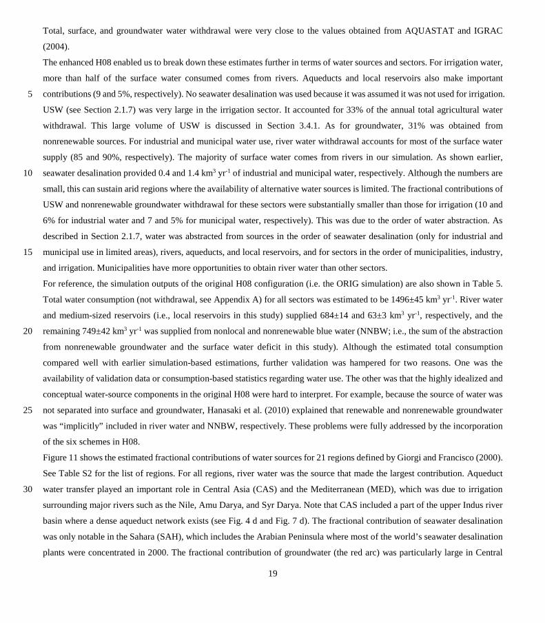
Figure 11 shows the estimated fractional contributions of water sources for 21 regions defined by Giorgi and Francisco (2000).

See Table S2 for the list of regions. For all regions, river water was the source that made the largest contribution. Aqueduct

water transfer played an important role in Central Asia (CAS) and the Mediterranean (MED), which was due to irrigation 30

surrounding major rivers such as the Nile, Amu Darya, and Syr Darya. Note that CAS included a part of the upper Indus river

basin where a dense aqueduct network exists (see Fig. 4 d and Fig. 7 d). The fractional contribution of seawater desalination

was only notable in the Sahara (SAH), which includes the Arabian Peninsula where most of the world’s seawater desalination

plants were concentrated in 2000. The fractional contribution of groundwater (the red arc) was particularly large in Central

20

North America (CNA), Central America (CAM), SAH, and South Asia (SAS). The fractional contribution of nonrenewable

groundwater, seawater desalination, and USW (the black arc) was particularly large in CNA, SAH, SAS, East Africa (EAF),

CAS, and Tibet (TIB). All of these are arid or semi-arid regions. Note that TIB included a major part of the Xinjiang Uyghur

Autonomous Region in China and part of northwestern India, with both having an arid and semi-arid climate and a vast

irrigation area. The black arc is marginal only for the regions in northern latitudes, such as Alaska (ALA), Greenland (GRL), 5

Northern Europe (NEU), and North Asia (NAS). The results indicate that further investigation is needed on the consistency

between the simulated water availability and use in mid to low latitudes.

3.4. Uncertainties

Although H08 has been substantially improved by incorporating the six schemes, uncertainties still remain. In this subsection,

we summarize the key uncertainties and challenges, with a particular focus on the terms USW and nonrenewable groundwater. 10

3.4.1. Unspecified surface water (USW)

The key precondition of H08 (and to the best of our knowledge all of the GHMs with human water abstraction) is that the water

requirement is first determined and, subsequently, water withdrawal from specific sources is estimated taking spatiotemporal

water availability into account. Hence, USW can be regarded as the inconsistency between the water availability and water 15

requirement. USW was simulated to be 747 km3yr-1 by introducing USW (see description of Option 1 in Section 2.1.7). As

shown in Table 5, the simulated total water withdrawal (3628 km3yr-1), which is identical to the water requirement when option

1 is taken for USW, was close to the reported global water withdrawal (3550 km3yr-1, AQUASTAT) and the fractional

contributions of surface water and groundwater were also close to the ratio reported by IGRAC (2004). However, in the H08

simulation the water requirement is not fulfilled by accessible surface water. 20

Figure 12 (a) shows the global distribution of USW. USW was extensively distributed in the Indian subcontinent, China, and

western North America, particularly concentrated in northern India, Pakistan, and coastal northern China. The majority of

USW was attributed to the shortage in surface irrigation water (Table 5).

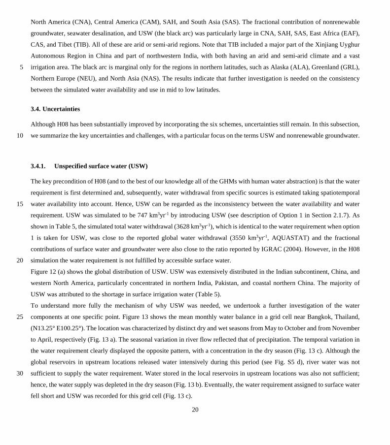
To understand more fully the mechanism of why USW was needed, we undertook a further investigation of the water

components at one specific point. Figure 13 shows the mean monthly water balance in a grid cell near Bangkok, Thailand, 25

(N13.25° E100.25°). The location was characterized by distinct dry and wet seasons from May to October and from November

to April, respectively (Fig. 13 a). The seasonal variation in river flow reflected that of precipitation. The temporal variation in

the water requirement clearly displayed the opposite pattern, with a concentration in the dry season (Fig. 13 c). Although the

global reservoirs in upstream locations released water intensively during this period (see Fig. S5 d), river water was not

sufficient to supply the water requirement. Water stored in the local reservoirs in upstream locations was also not sufficient; 30

hence, the water supply was depleted in the dry season (Fig. 13 b). Eventually, the water requirement assigned to surface water

fell short and USW was recorded for this grid cell (Fig. 13 c).

21

Figure 12 (b) shows the area supplied by global and local reservoirs. It shows the total storage capacity of all global and local

reservoirs in upstream locations divided by the number of seconds in a year, or the rate of flow if the reservoirs released all of

the stored water constantly during a year. The area supplied is extensive; however, compared with the area of USW (Fig. 12a),

the water stored in the reservoirs was not sufficient to fully meet the USW. For example, the USW was concentrated in

northwestern India and northeastern China, while only a few local reservoirs were located in these regions. 5

3.4.2. Nonrenewable groundwater

The estimation of the volume of abstracted nonrenewable groundwater contained considerable uncertainties. Although the

estimated volume of abstracted global total nonrenewable groundwater agreed well with earlier estimates (113-330 km3yr-1;

Table 5), the simulated trends of TWSA for selected basins, as shown in Fig. 10, tended to be overestimated. This contradiction

was largely attributed to the uncertainty in both the quantitative and geographic estimation of nonrenewable groundwater 10

usage. As shown in Fig. 6c, the national estimates still differed substantially from the earlier simulation-based estimates. These

results imply that nonrenewable groundwater might be overestimated to some extent.

3.4.3. Potential sources of uncertainty

There were four major sources of uncertainty in this study, which, potentially, caused the paradoxes of USW and nonrenewable

groundwater. The first was the limitation in the performance of physical hydrological sub-models. In particular, the rate of 15

river flow in the dry season and groundwater recharge influenced the simulation of water availability. Although the key

hydrological processes were represented, the land surface hydrology and river routing sub-models of H08 are relatively simple

(Appendix A). Moreover, the hydrological parameters were not tuned to individual basins, which yielding a generally lower

reproducibility of historical river flow observations (e.g. Hattermann et al., 2017). In cases in which the H08 model was

applied to specific basins, sensitivity testing and hydrological parameter calibration were conducted systematically using 20

reliable long-term observations (e.g. Hanasaki et al. 2014; Masood et al. 2015). Conversely, when H08 is applied globally, as

in this study, these procedures are difficult to perform because observations are not available for vast areas and simulation

periods. Without ground truthing, the sensitivity test cannot be interpreted, and parameter calibration cannot be performed.

This is particularly true for groundwater parameters because very few reliable observations representing the grid-cell size (i.e.

0.5° × 0.5°) are available. Also, the global climate data we used contained uncertainties. There are still considerable 25

discrepancies among the latest global meteorological data sets (e.g., Müller-Schmied et al., 2014), which implies that there are

regions where the input data are likely to be not well constrained by observations.

The second source of uncertainty was that H08 still omits some important water sources. They include, small ponds and

reservoirs, and melt water from glaciers. In this study, we accounted for 6852 major reservoirs, totaling 6197 km3 of storage

capacity, which were registered in the GRanD database as global and local reservoirs. Lehner et al. (2011) estimated that the 30

total number and water storage of reservoirs in the world is 16.7 million and 8070 km3, respectively, which implies

approximately 16 million and 2000 km3 minor ponds and reservoirs are still not accounted for in this study. No database of

22

such ponds and reservoirs has been developed yet, but if they were included, the temporal gap between water requirement and

availability would be further diminished. Glacier melt water, which was not considered in this study, might increase surface

water availability in some regions of the world, typically central Asia. Hirabayashi et al. (2010) estimated the annual global

total melt water from glaciers to be 19.8 km3 yr-1 (1990-2003). In addition, improvements are also needed for the aqueduct

database. Although aqueducts were considered in the model, the number and coverage of explicit aqueducts was less than the 5

actual situation.

The third source of uncertainty was that the models and algorithms for the water requirement. Because it is by far the largest

water user of the three sectors considered in the study, the estimation of irrigation water is crucially important. Probably the

largest assumption in H08 is that the irrigation water requirement is fully met (i.e., soil moisture is kept at a certain level; see

Appendix A) during the cropping period. This may overestimate the irrigation water requirement in arid and semi-arid climates 10

where deficit irrigation is practiced (Döll et al., 2014). We note that Siebert et al. (2015) developed the global distribution of

irrigated areas from 1900 to 2005, which would be an important contribution to simulations incorporating inter-annual

variations in the irrigation water requirement. We fixed the irrigated area throughout the simulation period, however, because

little information is available on annual variation in crop practice (e.g. crop type, fractions of surface water and groundwater

dependence). Further incorporation of local agricultural practices into the model is crucial to improve its performance. This 15

includes crop type, cultivars, planting, and harvesting date, timing and intensity of irrigation, permitted water use, and

irrigation equipment, all of which affect the temporal variation and volume of the irrigation water requirement. Water source

separation into surface and ground water is determined by the single factor termed the fraction of water requirement to

groundwater. Due to lack of data availability, the same factor is applied for vast areas ignoring the actual local heterogeneity

which is also a source of uncertainty. 20

The fourth source of uncertainty regards spatiotemporal resolution, which should be further investigated. It was a fundamental

presumption of this study that the minimum temporal and spatial unit of hydrology and water use was one day and one 0.5° ×

0.5° grid cell. A further increase in spatiotemporal resolution would enhance the use of return flow, which would increase the

gross water availability.

4. Conclusions 25

Six schemes were added to the H08 model to represent human water abstraction more accurately and ensure the all water fluxes

and storage are traceable in each grid cell at a daily interval. Our model indicated that in the year 2000, of a total freshwater

abstraction of 3628 km3yr-1, 2839 km3yr-1 was from surface water and 789 km3yr-1 was from groundwater. Streamflow,

aqueducts, local reservoirs, and seawater desalination accounted for 1786, 199, 106, and 1.8 km3yr-1 of the surface water,

respectively, while 747 km3yr-1 of surface water requirement was unmet. Renewable and nonrenewable groundwater 30

accounted for 607 and 182 km3yr-1, respectively. These estimations agreed well with earlier studies that were based on

23

statistics and simulations. Furthermore, the incorporation of these six schemes improved the river discharge and TWSA

simulations in heavily human-affected basins.

Every water source differed in its renewability, economic costs for development, and environmental consequences for usage.

To cope with the increasing water requirement and changing climate in the 21st century, efficient water management is

crucially important all over the world. The enhanced H08 model can incorporate the aspects of sustainability, economy, and 5

environment into forthcoming global water resource assessments.

Among the six schemes, local reservoirs, aqueduct water transfer, and seawater desalination were incorporated into GHMs for

the first time, to the best of our knowledge. The key concept of a local reservoir is that of isolating the storage of reservoirs in

tributaries from global river systems. This is a practical way to express the role of small reservoirs in the limited spatial

resolution of a GHM. The aqueduct water transfer scheme enables water from major rivers to be distributed to surrounding grid 10

cells. Because a comprehensive digital global inventory of aqueducts is not currently available, the scheme includes an

algorithm to infer the potential routes of aqueducts. This scheme reduces the gap in water availability in the grid cells between

periods when the major rivers are flowing and when they are not. This function is potentially useful in high-resolution water

resource modeling (e.g., Wada et al., 2016), although inter-cell water transfer is a key technical issue that needs to be resolved.

The seawater desalination scheme enables the intensive water-use taking place in some of the arid coastal regions (e.g., the 15

Gulf countries) to be explained. Although the contribution of seawater desalination is currently limited in terms of quantity and

spatial extent, it could expand considerably due to socio-economic conditions and climate change (Hanasaki et al., 2016).

Acknowledgment

This work was mainly supported by the Japan Society for the Promotion of Science (JSPS) KAKENHI Grant Number

16H06291. It was partially supported by JSPS KAKENHI Grant Number 25820230, the Environment Research and 20

Technology Development Fund (S-14) of the Ministry of the Environment, Japan, and the Core Research for Evolutionary

Science and Technology (CREST), Japan Science and Technology Agency. The present work was partially developed within

the framework of the Panta Rhei Research Initiative of the International Association of Hydrological Sciences (IAHS) by the

Water Scarcity Assessment: Methodology and Application working group. The authors thank Yoshihide Wada for providing

technical details regarding PCR-GLOBWB and Hodaka Kamoshida for technical assistance with handling GIS data. Map 25

colors were based on www.ColorBrewer.org, by Cynthia A. Brewer, Penn State. Observed runoff data were kindly provided by

the Global Runoff Data Centre, 56068 Koblenz, Germany.

Appendix A

The H08 model is a grid-cell based GHM. Although the name H08 is used to refer to “a model described in Hanasaki et al.

(2008a,b)”, we also included additional sub-models described in Hanasaki et al. (2010 and 2013a,b) in H08. The H08 model 30

24

has been used in several advanced global water-resource assessments to assess water scarcity globally, with consideration

given to the seasonality of water availability and use, in historical periods (Hanasaki et al. 2008b) and future periods under

comprehensive global change scenarios (Hanasaki et al. 2013a,b). It has also been used to estimate the global flow of so-called

‘virtual water’, providing details of the sources of water and their temporal evolution (Hanasaki et al., 2010; Hanasaki, 2016;

Dalin et al., 2012). The model has participated in major international model inter-comparison projects, such as EU Water and 5

Global Change (EU-WATCH; Haddeland et al., 2011) and Inter-Sectoral Impact Model Intercomparison Project (ISIMIP;

Schewe et al., 2014; Haddeland et al., 2014), to identify its strengths and weaknesses among the other influential models that

are currently available. Recently, H08 has been applied in regional domains, with calibrated hydrological parameters

(Hanasaki et al., 2014; Mateo et al., 2014; Masood et al., 2015).

The original H08 model consists of six sub-models, namely land surface, river routing, reservoir operation, crop growth, 10

environmental flow, and water abstraction. The formulations of these sub-models are described in detail in Hanasaki et al.

(2008a,b, 2010). In the standard simulation settings, H08 covers the whole globe at a resolution of 1° × 1° or 0.5° × 0.5° to

assess the geographical heterogeneity of hydrology and water use. Typically, the simulation period is several decades and the

calculation interval is one day. The six sub-models exchange water fluxes and update the water storage at each calculation

interval, with no unexplained water balance (the error is less than 0.01% of the total input precipitation). These characteristics 15

have enabled explicit simulations of the major interactions between the natural water cycle and major human activities around

the globe. The source code and H08 manuals are open to the public, and are available at http://h08.nies.go.jp.

The land surface sub-model is a bucket model (Manabe et al., 1969; Robock et al., 1995), with a simple drainage scheme that

generates subsurface runoff (Gerten et al., 2004). It solves the energy balance of the land surface and the water balance of the

top 1 m of soil. It estimates surface runoff, which is generated when the soil is saturated, and subsurface runoff, which is 20

generated regularly as a function of soil moisture. A land grid cell is subdivided into four sub-cells to represent the different

land uses, namely, double-crop irrigated, single-crop irrigated, rainfed cropland, and non-cropland. The fractional

contributions of each sub-cell are determined by the specific geographical maps listed in Table 1. The river routing sub-model

is a simple scheme to transport total runoff (sum of surface and subsurface runoff) through the digital grid-based river network

(Oki et al., 1999). When a river section includes large reservoirs (LRs; corresponding to global reservoirs in this study), the 25

river flow is regulated following the specific reservoir operation rule generated by the reservoir operation sub-model. LRs are

defined as reservoirs with more than 1 km3 of total storage capacity (Hanasaki et al., 2006). LRs, which total 507 in number and

4411 km3 in storage capacity, are explicitly georeferenced in the digital river network of H08. The crop growth sub-model

plays two roles. One is to estimate the planting date of crops globally. This is done by the use of a stand-alone crop growth

model prior to a H08 hydrological simulation, using the planting and harvesting date in a year that yields maximum crop 30

production. The other role is to simulate crop growth during a H08 hydrological simulation, which provides the daily status of

cultivation for use in the water abstraction sub-model. The environmental flow sub-model estimates the river flow that should

be kept in the river channel for the aquatic ecosystem. The water abstraction sub-model, which was the main concern of this

study, is described in detail in the next paragraph.

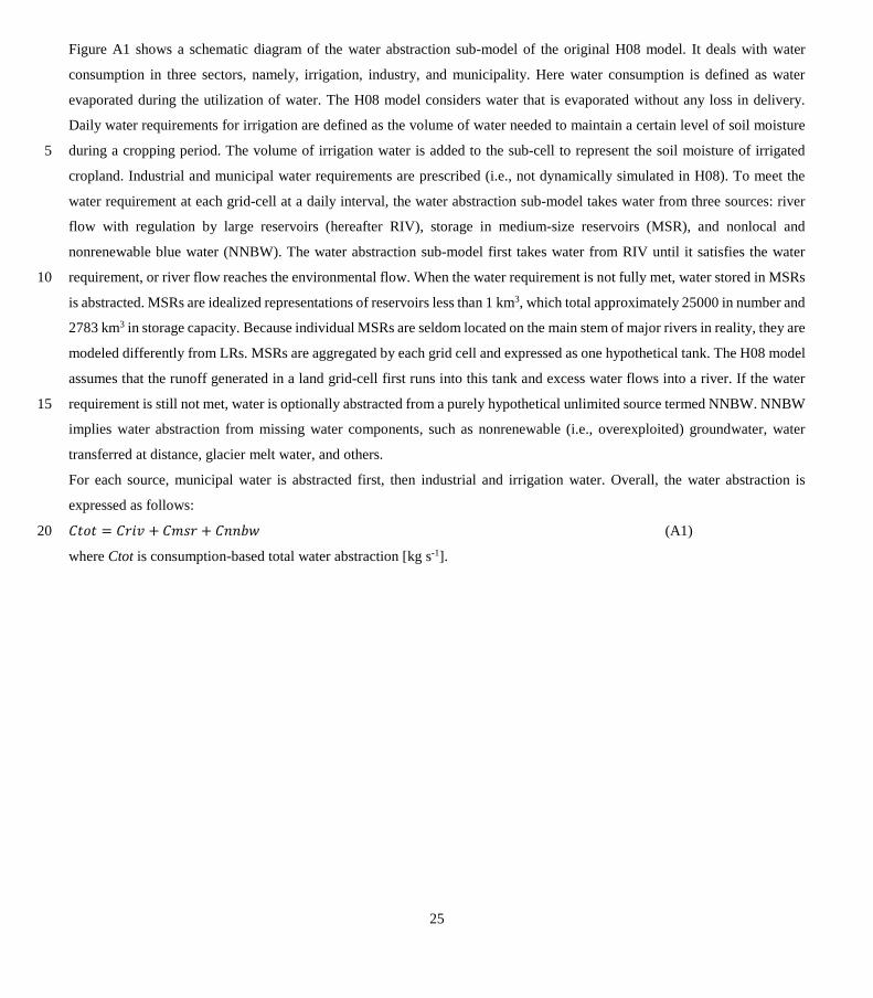
25

Figure A1 shows a schematic diagram of the water abstraction sub-model of the original H08 model. It deals with water

consumption in three sectors, namely, irrigation, industry, and municipality. Here water consumption is defined as water

evaporated during the utilization of water. The H08 model considers water that is evaporated without any loss in delivery.

Daily water requirements for irrigation are defined as the volume of water needed to maintain a certain level of soil moisture

during a cropping period. The volume of irrigation water is added to the sub-cell to represent the soil moisture of irrigated 5

cropland. Industrial and municipal water requirements are prescribed (i.e., not dynamically simulated in H08). To meet the

water requirement at each grid-cell at a daily interval, the water abstraction sub-model takes water from three sources: river

flow with regulation by large reservoirs (hereafter RIV), storage in medium-size reservoirs (MSR), and nonlocal and

nonrenewable blue water (NNBW). The water abstraction sub-model first takes water from RIV until it satisfies the water

requirement, or river flow reaches the environmental flow. When the water requirement is not fully met, water stored in MSRs 10

is abstracted. MSRs are idealized representations of reservoirs less than 1 km3, which total approximately 25000 in number and

2783 km3 in storage capacity. Because individual MSRs are seldom located on the main stem of major rivers in reality, they are

modeled differently from LRs. MSRs are aggregated by each grid cell and expressed as one hypothetical tank. The H08 model

assumes that the runoff generated in a land grid-cell first runs into this tank and excess water flows into a river. If the water

requirement is still not met, water is optionally abstracted from a purely hypothetical unlimited source termed NNBW. NNBW 15

implies water abstraction from missing water components, such as nonrenewable (i.e., overexploited) groundwater, water

transferred at distance, glacier melt water, and others.

For each source, municipal water is abstracted first, then industrial and irrigation water. Overall, the water abstraction is

expressed as follows:

𝐶𝐶𝑄𝑄𝑄𝑄𝑄𝑄 = 𝐶𝐶𝑄𝑄𝑚𝑚𝑊𝑊 + 𝐶𝐶𝑚𝑚𝐴𝐴𝑄𝑄 + 𝐶𝐶𝑚𝑚𝑚𝑚𝑄𝑄𝑊𝑊 (A1) 20

where Ctot is consumption-based total water abstraction [kg s-1].

26

References

Alcamo, J., Döll, P., Henrichs, T., Kaspar, F., Lehner, B., Rösch, T., and Siebert, S.: Development and testing of the

WaterGAP 2 global model of water use and availability, Hydrolog. Sci. J., 48, 317-337, 10.1623/hysj.48.3.317.45290,

2003.

Amante, C., and Eakins, B. W.: ETOPO1 1 Arc-Minute Global Relief Model: Procedures, Data Sources and Analysis, National 5

Geophysical Data Center, NOAA. NOAA Technical Memorandum NESDIS NGDC-24, 19, 2009.

Biemans, H., Haddeland, I., Kabat, P., Ludwig, F., Hutjes, R. W. A., Heinke, J., von Bloh, W., and Gerten, D.: Impact of

reservoirs on river discharge and irrigation water supply during the 20th century, Water Resour. Res., 47, W03509,

10.1029/2009wr008929, 2011.

Bierkens, M. F. P.: Global hydrology 2015: State, trends, and directions, Water Resour. Res., 51, 4923-4947, 10

10.1002/2015WR017173, 2015.

Brown, J., Ferrians, O., Heginbottom, J. A., and Melnikov, E.: Circum-Arctic Map of Permafrost and Ground-Ice Conditions,

Version 2, National Snow and Ice Data Center, Boulder, Colorado USA, 2002.

Center for International Earth Science Information Network (CIESIN) Columbia University, and Centro Internacional de

Agricultura Tropical (CIAT): Gridded Population of the World Version 3 (GPWv3): Population Grids, Socioeconomic 15

Data and Applications Center (SEDAC) Columbia University, Palisades, NY, 2005.

Dalin, C., Konar, M., Hanasaki, N., Rinaldo, A., and Rodriguez-Iturbe, I.: Evolution of the global virtual water trade network,

P. Natl. Acad. Sci. USA, 109, 5989-5994, 10.1073/pnas.1203176109, 2012.

Dirmeyer, P. A., Gao, X. A., Zhao, M., Guo, Z. C., Oki, T. K., and Hanasaki, N.: GSWP-2 - Multimodel analysis and

implications for our perception of the land surface, B. Am. Meteorol. Soc., 87, 1381-1397, 10.1175/BAMS-87-10-1381, 20

2006.

Döll, P., and Siebert, S.: Global modeling of irrigation water requirements, Water Resour. Res., 38, 1037,

10.1029/2001WR000355, 2002.

Döll, P., Lehner, B., and Kaspar, F.: Global Modeling of Groundwater Recharge, in Proceedings of Third International

Conference on Water Resources and the Environment Research, Technical University of Dresden, Germany, 27-31, 25

2002.

Döll, P., Kaspar, F., and Lehner, B.: A global hydrological model for deriving water availability indicators: model tuning and

validation, J. Hydrol., 270, 105-134, 10.1016/S0022-1694(02)00283-4, 2003.

Döll, P., and Fiedler, K.: Global-scale modeling of groundwater recharge, Hydrol. Earth Syst. Sci., 12, 863-885,

10.5194/hess-12-863-2008, 2008. 30

Döll, P., Fiedler, K., and Zhang, J.: Global-scale analysis of river flow alterations due to water withdrawals and reservoirs,

Hydrol. Earth Syst. Sci., 13, 2413-2432, 10.5194/hess-13-2413-2009, 2009.

27

Döll, P., Hoffmann-Dobrev, H., Portmann, F. T., Siebert, S., Eicker, A., Rodell, M., Strassberg, G., and Scanlon, B. R.: Impact

of water withdrawals from groundwater and surface water on continental water storage variations, J. Geodyn, 59–60,

143-156, 10.1016/j.jog.2011.05.001, 2012.

Döll, P., Müller Schmied, H., Schuh, C., Portmann, F. T., and Eicker, A.: Global-scale assessment of groundwater depletion

and related groundwater abstractions: Combining hydrological modeling with information from well observations and 5

GRACE satellites, Water Resour. Res., 50, 5698-5720, 10.1002/2014wr015595, 2014.

Fan, Y., Miguez-Macho, G., Weaver, C. P., Walko, R., and Robock, A.: Incorporating water table dynamics in climate

modeling: 1. Water table observations and equilibrium water table simulations, Journal of Geophysical Research:

Atmospheres, 112, D10125, 10.1029/2006JD008111, 2007.

FAO, IIASA, ISRIC, ISSCAS, and JRC: Harmonized World Soil Database (version 1.2), FAO, Rome, Italy, IIASA, 10

Laxenburg, Austria, 2012.

Flörke, M., Kynast, E., Bärlund, I., Eisner, S., Wimmer, F., and Alcamo, J.: Domestic and industrial water uses of the past 60

years as a mirror of socio-economic development: A global simulation study, Global Environ. Chang., 23, 144-156,

10.1016/j.gloenvcha.2012.10.018, 2013.

Feitelson, E. and Rosenthal, G.: Desalination, space and power: The ramifications of Israel’s changing water geography, 15

Geoforum, 43, 2, 272-284, 10.1016/j.geoforum.2011.08.011, 2012.

Gerten, D., Schaphoff, S., Haberlandt, U., Lucht, W., and Sitch, S.: Terrestrial vegetation and water balance - hydrological

evaluation of a dynamic global vegetation model, J. Hydrol., 286, 249-270, 10.1016/j.jhydrol.2003.09.029, 2004.

Ghaffour, N., Missimer, T. M., and Amy, G. L.: Technical review and evaluation of the economics of water desalination:

Current and future challenges for better water supply sustainability, Desalination, 309, 197-207, 20

10.1016/j.desal.2012.10.015, 2013.

Giorgi, F., and Francisco, R.: Uncertainties in regional climate change prediction: a regional analysis of ensemble simulations

with the HADCM2 coupled AOGCM, Clim. Dyn., 16, 169-182, 10.1007/pl00013733, 2000.

Haddeland, I., Lettenmaier, D. P., and Skaugen, T.: Effects of irrigation on the water and energy balances of the Colorado and

Mekong river basins, J. Hydrol., 324, 210-223, 10.1016/j.jhydrol.2005.09.028, 2006. 25

Haddeland, I., Clark, D. B., Franssen, W., Ludwig, F., Voß, F., Arnell, N. W., Bertrand, N., Best, M., Folwell, S., Gerten, D.,

Gomes, S., Gosling, S. N., Hagemann, S., Hanasaki, N., Harding, R., Heinke, J., Kabat, P., Koirala, S., Oki, T., Polcher,

J., Stacke, T., Viterbo, P., Weedon, G. P., and Yeh, P.: Multimodel Estimate of the Global Terrestrial Water Balance:

Setup and First Results, J. Hydromet., 12, 869-884, 10.1175/2011jhm1324.1, 2011.

Haddeland, I., Heinke, J., Biemans, H., Eisner, S., Flörke, M., Hanasaki, N., Konzmann, M., Ludwig, F., Masaki, Y., Schewe, 30

J., Stacke, T., Tessler, Z. D., Wada, Y., and Wisser, D.: Global water resources affected by human interventions and

climate change, P. Natl. Acad. Sci. USA, 111, 3251-3256, 10.1073/pnas.1222475110, 2014.

Hanasaki, N., Kanae, S., and Oki, T.: A reservoir operation scheme for global river routing models, J. Hydrol., 327, 22-41,

10.1016/j.jhydrol.2005.11.011, 2006.

28

Hanasaki, N., Kanae, S., Oki, T., Masuda, K., Motoya, K., Shirakawa, N., Shen, Y., and Tanaka, K.: An integrated model for

the assessment of global water resources - Part 1: Model description and input meteorological forcing, Hydrol. Earth Syst.

Sci., 12, 1007-1025, 10.5194/hess-12-1007-2008, 2008a.

Hanasaki, N., Kanae, S., Oki, T., Masuda, K., Motoya, K., Shirakawa, N., Shen, Y., and Tanaka, K.: An integrated model for

the assessment of global water resources - Part 2: Applications and assessments, Hydrol. Earth Syst. Sci., 12, 1027-1037, 5

10.5194/hess-12-1027-2008, 2008b.

Hanasaki, N., Inuzuka, T., Kanae, S., and Oki, T.: An estimation of global virtual water flow and sources of water withdrawal

for major crops and livestock products using a global hydrological model, J. Hydrol., 384, 232-244,

10.1016/j.jhydrol.2009.09.028, 2010.

Hanasaki, N., Fujimori, S., Yamamoto, T., Yoshikawa, S., Masaki, Y., Hijioka, Y., Kainuma, M., Kanamori, Y., Masui, T., 10

Takahashi, K., and Kanae, S.: A global water scarcity assessment under Shared Socio-economic Pathways – Part 1:

Water use, Hydrol. Earth Syst. Sci., 17, 2375-2391, 10.5194hess-17-2375-2013, 2013a.

Hanasaki, N., Fujimori, S., Yamamoto, T., Yoshikawa, S., Masaki, Y., Hijioka, Y., Kainuma, M., Kanamori, Y., Masui, T.,

Takahashi, K., and Kanae, S.: A global water scarcity assessment under Shared Socio-economic Pathways – Part 2:

Water availability and scarcity, Hydrol. Earth Syst. Sci., 17, 2393-2413, 10.5194/hess-17-2393-2013, 2013b. 15

Hanasaki, N., Saito, Y., Chaiyasaen, C., Champathong, A., Ekkawatpanit, C., Saphaokham, S., Sukhapunnaphan, T., Sumdin,

S., and Thongduang, J.: A quasi-real-time hydrological simulation of the Chao Phraya River using meteorological data

from the Thai Meteorological Department Automatic Weather Stations, Hydrological Research Letters, 8, 9-14,

10.3178/hrl.8.9, 2014.

Hanasaki, N.: Estimating Virtual Water Contents Using a Global Hydrological Model: Basis and applications, in: Terrestrial 20

Water Cycle and Climate Change: Natural and Human-Induced Impacts, edited by: Tang, Q., and Oki, T., John Wiley &

Sons, Inc., 209-228, 2016.

Hanasaki, N., Yoshikawa, S., Kakinuma, K., and Kanae, S.: A seawater desalination scheme for global hydrological models,

Hydrol. Earth Syst. Sci., 20, 4143-4157, 10.5194/hess-20-4143-2016, 2016.

Hattermann, F. F., Krysanova, V., Gosling, S. N., Dankers, R., Daggupati, P., Donnelly, C., Flörke, M., Huang, S., Motovilov, 25

Y., Buda, S., Yang, T., Müller, C., Leng, G., Tang, Q., Portmann, F. T., Hagemann, S., Gerten, D., Wada, Y., Masaki, Y.,

Alemayehu, T., Satoh, Y., and Samaniego, L.: Cross‐scale intercomparison of climate change impacts simulated by

regional and global hydrological models in eleven large river basins, Climatic Change, 141, 561-576,

10.1007/s10584-016-1829-4, 2017.

Healey, R. W.: Estimating ground water recharge, Cambridge University Press, Cambridge, UK, 245 pp.245, 2010. 30

Hirabayashi, Y., Döll, P., and Kanae, S.: Global-scale modeling of glacier mass balances for water resources assessments:

Glacier mass changes between 1948 and 2006, J. Hydrol., 390, 245-256, 10.1016/j.jhydrol.2010.07.001, 2010.

International Groundwater Resources Assessment Centre (IGRAC): Global Groundwater Information System (GGIS), 2004.

29

Jägermeyr, J., Gerten, D., Heinke, J., Schaphoff, S., Kummu, M., and Lucht, W.: Water savings potentials of irrigation

systems: global simulation of processes and linkages, Hydrol. Earth Syst. Sci., 19, 3073-3091,

10.5194/hess-19-3073-2015, 2015.

Koirala, S., Yeh, P. J. F., Hirabayashi, Y., Kanae, S., and Oki, T.: Global-scale land surface hydrologic modeling with the

representation of water table dynamics, Journal of Geophysical Research: Atmospheres, 119, 75-89, 5

10.1002/2013JD020398, 2014.

Konikow, L. F.: Contribution of global groundwater depletion since 1900 to sea-level rise, Geophys. Res. Lett., 38, L17401,

10.1029/2011gl048604, 2011.

Landerer, F. W., and Swenson, S. C.: Accuracy of scaled GRACE terrestrial water storage estimates, Water Resour. Res., 48,

W04531, 10.1029/2011WR011453, 2012. 10

Lehner, B., Verdin, K., and Jarvis, A.: New global hydrography derived from spaceborne elevation data. , Eos Trans AGU 89:,

93-94, 2008.

Lehner, B., Liermann, C. R., Revenga, C., Vörösmarty, C., Fekete, B., Crouzet, P., Döll, P., Endejan, M., Frenken, K.,

Magome, J., Nilsson, C., Robertson, J. C., Rödel, R., Sindorf, N., and Wisser, D.: High-resolution mapping of the world's

reservoirs and dams for sustainable river-flow management, Front Ecol Environ, 9, 494-502, 10.1890/100125, 2011. 15

Manabe, S.: Climate and the ocean circulation 1. The atmospheric circulation and the hydrology of the earth's surface, Mon.

Weather Rev., 97, 739-774, 10.1175/1520-0493(1969)097<0739:CATOC>2.3.CO;2, 1969.

Margat, J., and van der Gun, J.: Groundwater around the world, Taylor & Francis Group, London, UK, 348 pp., 2013.

Masood, M., Yeh, P. J. F., Hanasaki, N., and Takeuchi, K.: Model study of the impacts of future climate change on the

hydrology of Ganges–Brahmaputra–Meghna basin, Hydrol. Earth Syst. Sci., 19, 747-770, 10.5194/hess-19-747-2015, 20

2015.

Mateo, C. M., Hanasaki, N., Komori, D., Tanaka, K., Kiguchi, M., Champathong, A., Sukhapunnaphan, T., Yamazaki, D., and

Oki, T.: Assessing the impacts of reservoir operation to floodplain inundation by combining hydrological, reservoir

management, and hydrodynamic models, Water Resour. Res., 50, 7245-7266, 10.1002/2013wr014845, 2014.

Mingzhou, Q., Jackson, R. H., Zhongjin, Y., Jackson, M. W., and Bo, S.: The effects of sediment-laden waters on irrigated 25

lands along the lower Yellow River in China, J. Environ Manage, 85, 858-865, 10.1016/j.jenvman.2006.10.015, 2007.

Monfreda, C., Ramankutty, N., and Foley, J. A.: Farming the Planet. Part 2: The Geographic Distribution of Crop Areas and

Yields in the Year 2000, Glob. Biogeochem. Cycles, 22, GB1022, 10.1029/2007GB002947, 2008.

Müller Schmied, H., Eisner, S., Franz, D., Wattenbach, M., Portmann, F. T., Flörke, M., and Döll, P.: Sensitivity of simulated

global-scale freshwater fluxes and storages to input data, hydrological model structure, human water use and calibration, 30

Hydrol. Earth Syst. Sci., 18, 3511-3538, 10.5194/hess-18-3511-2014, 2014.

Nash, J. E., and Sutcliffe, J. V.: River flow forecasting through conceptual models part I — A discussion of principles, J.

Hydrol., 10, 282-290, 10.1016/0022-1694(70)90255-6, 1970.

30

Nazemi, A., and Wheater, H. S.: On inclusion of water resource management in Earth system models - Part 1: Problem

definition and representation of water demand, Hydrol. Earth Syst. Sci., 19, 33-61, 10.5194/hess-19-33-2015, 2015.

Nazemi, A., and Wheater, H. S.: On inclusion of water resource management in Earth system models - Part 2: Representation

of water supply and allocation and opportunities for improved modeling, Hydrol. Earth Syst. Sci., 19, 63-90,

10.5194/hess-19-63-2015, 2015. 5

National Water Development Agency (NWDA): Inter Basin Water Transfer Links, available at

http://www.nwda.gov.in/index.asp?langid=1 (last access: 1 June, 2016), 2016.

National Water Resources Plan Egypt (NWRP): Water for the Future, National Water Resources Plan for Egypt 2017, 2005.

Niu, G.-Y., Yang, Z.-L., Dickinson, R. E., Gulden, L. E., and Su, H.: Development of a simple groundwater model for use in

climate models and evaluation with Gravity Recovery and Climate Experiment data, Journal of Geophysical Research: 10

Atmospheres, 112, D07103, 10.1029/2006JD007522, 2007.

Oki, T., Nishimura, T., and Dirmeyer, P.: Assessment of annual runoff from land surface models using Total Runoff

Integrating Pathways (TRIP), J. Meteorol. Soc. Jpn., 77, 235-255, 10.2151/jmsj1965.77.1B_235, 1999.

Oki, T., Agata, Y., Kanae, S., Saruhashi, T., Yang, D. W., and Musiake, K.: Global assessment of current water resources using

total runoff integrating pathways, Hydrolog. Sci. J., 46, 983-995, 10.1080/02626660109492890, 2001. 15

Oki, T., and Kanae, S.: Global Hydrological Cycles and World Water Resources, Science, 313, 1068-1072,

10.1126/science.1128845, 2006.

Pokhrel, Y., Hanasaki, N., Koirala, S., Cho, J., Yeh, P. J. F., Kim, H., Kanae, S., and Oki, T.: Incorporating Anthropogenic

Water Regulation Modules into a Land Surface Model, J. Hydromet., 13, 255-269, 10.1175/jhm-d-11-013.1, 2012a.

Pokhrel, Y. N., Hanasaki, N., Yeh, P. J. F., Yamada, T. J., Kanae, S., and Oki, T.: Model estimates of sea-level change due to 20

anthropogenic impacts on terrestrial water storage, Nature Geosci., 5, 389-392, 10.1038/ngeo1476, 2012b.

Pokhrel, Y. N., Koirala, S., Yeh, P. J. F., Hanasaki, N., Longuevergne, L., Kanae, S., and Oki, T.: Incorporation of groundwater

pumping in a global Land Surface Model with the representation of human impacts, Water Resour. Res., 51, 78-96,

10.1002/2014wr015602, 2015.

Pokhrel, Y. N., Hanasaki, N., Wada, Y., and Kim, H.: Recent progresses in incorporating human land–water management into 25

global land surface models toward their integration into Earth system models, Wiley Interdisciplinary Reviews: Water, 3,

548-574, 10.1002/wat2.1150, 2016.

Postel, S.: Pillar of sand -Can the irrigation miracle last?, W.W. Norton and Company, Inc., New York, USA, 1999.

Richards, L. A.: Capillary conduction of liquids through porous mediums, Physics, 1, 318-333, 10.1063/1.1745010, 1931.

Robock, A., Vinnikov, K. Y., Schlosser, C. A., Speranskaya, N. A., and Xue, Y. K.: Use of Midlatitude Soil-Moisture and 30

Meteorological Observations to Validate Soil-Moisture Simulations with Biosphere and Bucket Models, J. Clim., 8,

15-35, 10.1175/1520-0442(1995)008<0015:UOMSMA>2.0.CO;2, 1995.

Rost, S., Gerten, D., Bondeau, A., Lucht, W., Rohwer, J., and Schaphoff, S.: Agricultural green and blue water consumption

and its influence on the global water system, Water Resour. Res., 44, W09405, 10.1029/2007WR006331, 2008.

31

Schewe, J., Heinke, J., Gerten, D., Haddeland, I., Arnell, N. W., Clark, D. B., Dankers, R., Eisner, S., Fekete, B. M.,

Colón-González, F. J., Gosling, S. N., Kim, H., Liu, X., Masaki, Y., Portmann, F. T., Satoh, Y., Stacke, T., Tang, Q.,

Wada, Y., Wisser, D., Albrecht, T., Frieler, K., Piontek, F., Warszawski, L., and Kabat, P.: Multimodel assessment of

water scarcity under climate change, P. Natl. Acad. Sci. USA, 111, 3245-3250, 10.1073/pnas.1222460110, 2014.

Shiklomanov, I. A.: Appraisal and assessment of world water resources, Water Int., 25, 11-32, 10.1080/02508060008686794, 5

2000.

Siebert, S., Döll, P., Hoogeveen, J., Faures, J. M., Frenken, K., and Feick, S.: Development and validation of the global map of

irrigation areas, Hydrol. Earth Syst. Sci., 9, 535-547, 10.5194/hess-9-535-2005, 2005.

Siebert, S., Burke, J., Faures, J. M., Frenken, K., Hoogeveen, J., Döll, P., and Portmann, F. T.: Groundwater use for irrigation

– a global inventory, Hydrol. Earth Syst. Sci., 14, 1863-1880, 10.5194hess-14-1863-2010, 2010. 10

Siebert, S., Kummu, M., Porkka, M., Döll, P., Ramankutty, N., and Scanlon, B. R.: A global data set of the extent of irrigated

land from 1900 to 2005, Hydrol. Earth Syst. Sci., 19, 1521-1545, 10.5194/hess-19-1521-2015, 2015.

Sood, A., and Smakhtin, V.: Global hydrological models: a review, Hydrolog. Sci. J., 60, 549-565,

10.1080/02626667.2014.950580, 2015.

State Water Project (SWP): The California State Water Project, available at http://www.water.ca.gov/swp/docs/SWPmap.pdf 15

(last access: 1 June, 2016), 2016.

Ullah, M. K., Habib, Z. and Muhammad, S.: Spatial distribution of reference and potential evapotranspiration across the Indus

Basin Irrigation Systems. Lahore, Pakistan: International Water Management Institute (IWMI working paper 24), 2011.

van Beek, L. P. H., and Bierkens, M. F. P.: The Global Hydrological Model PCR-GLOBWB: Conceptualization,

Parameterization and Verification, Department of Physical Geography, Utrecht University, Utrecht, The Netherlands, 20

2008.

van Beek, L. P. H., Wada, Y., and Bierkens, M. F. P.: Global monthly water stress: 1. Water balance and water availability,

Water Resour. Res., 47, W07517, 10.1029/2010wr009791, 2011.

Vörösmarty, C. J., Moore III, B., Grace, A. L., Gildea, M. P., Melillo, J. M., Peterson, B. J., Rastetter, E. B., and Steudler, P.

A.: Continental scale models of water balance and fluvial transport: An application to South America, Global 25

Biogeochem. Cy., 3-3, 241-265, 10.1029/GB003i003p00241, 1989.

Wada, Y., van Beek, L. P. H., van Kempen, C. M., Reckman, J. W. T. M., Vasak, S., and Bierkens, M. F. P.: Global depletion

of groundwater resources, Geophys. Res. Lett., 37, L20402, 10.1029/2010GL044571 2010.

Wada, Y., van Beek, L. P. H., Viviroli, D., Dürr, H. H., Weingartner, R., and Bierkens, M. F. P.: Global monthly water stress:

2. Water demand and severity of water stress, Water Resour. Res., 47, W07518, 10.1029/2010wr009792, 2011. 30

Wada, Y., Wisser, D., and Bierkens, M. F. P.: Global modeling of withdrawal, allocation and consumptive use of surface water

and groundwater resources, Earth Syst. Dynam., 5, 15-40, 10.5194/esd-5-15-2014, 2014.

Wada, Y., de Graaf, I. E. M., and van Beek, L. P. H.: High-resolution modeling of human and climate impacts on global water

resources, Journal of Advances in Modeling Earth Systems, 8, 735-763, 10.1002/2015MS000618, 2016.

32

Wada, Y.: Modeling Groundwater Depletion at Regional and Global Scales: Present State and Future Prospects, Surveys in

Geophysics, 37, 419-451, 10.1007/s10712-015-9347-x, 2016.

Weedon, G. P., Balsamo, G., Bellouin, N., Gomes, S., Best, M. J., and Viterbo, P.: The WFDEI meteorological forcing data

set: WATCH Forcing Data methodology applied to ERA-Interim reanalysis data, Water Resour. Res., 50, 7505-7514,

10.1002/2014WR015638, 2014. 5

Wisser, D., Fekete, B. M., Vörösmarty, C. J., and Schumann, A. H.: Reconstructing 20th century global hydrography: a

contribution to the Global Terrestrial Network- Hydrology (GTN-H), Hydrol. Earth Syst. Sci., 14, 1-24,

10.5194/hess-14-1-2010, 2010.

Yeh, P. J.-F., and Eltahir, E. A. B.: Representation of Water Table Dynamics in a Land Surface Scheme. Part I: Model

Development, J. Climate, 18, 1861-1880, 10.1175/jcli3330.1, 2005. 10

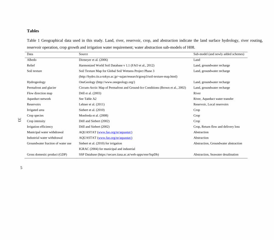
33

Tables

Table 1 Geographical data used in this study. Land, river, reservoir, crop, and abstraction indicate the land surface hydrology, river routing,

reservoir operation, crop growth and irrigation water requirement; water abstraction sub-models of H08. Data Source Sub-model (and newly added schemes)

Albedo Dirmeyer et al. (2006) Land

Relief Harmonized World Soil Database v 1.1 (FAO et al., 2012) Land, groundwater recharge

Soil texture Soil Texture Map for Global Soil Wetness Project Phase 3

(http://hydro.iis.u-tokyo.ac.jp/~sujan/research/gswp3/soil-texture-map.html)

Land, groundwater recharge

Hydrogeology OneGeology (http://www.onegeology.org/) Land, groundwater recharge

Permafrost and glacier Circum-Arctic Map of Permafrost and Ground-Ice Conditions (Brown et al., 2002) Land, groundwater recharge

Flow direction map Döll et al. (2003) River

Aqueduct network See Table A2 River, Aqueduct water transfer

Reservoirs Lehner et al. (2011) Reservoir, Local reservoirs

Irrigated area Siebert et al. (2010) Crop

Crop species Monfreda et al. (2008) Crop

Crop intensity Döll and Siebert (2002) Crop

Irrigation efficiency Döll and Siebert (2002) Crop, Return flow and delivery loss

Municipal water withdrawal AQUASTAT (www.fao.org/nr/aquastat/) Abstraction

Industrial water withdrawal AQUASTAT (www.fao.org/nr/aquastat/) Abstraction

Groundwater fraction of water use Siebert et al. (2010) for irrigation

IGRAC (2004) for municipal and industrial

Abstraction, Groundwater abstraction

Gross domestic product (GDP) SSP Database (https://secure.iiasa.ac.at/web-apps/ene/SspDb) Abstraction, Seawater desalination

5

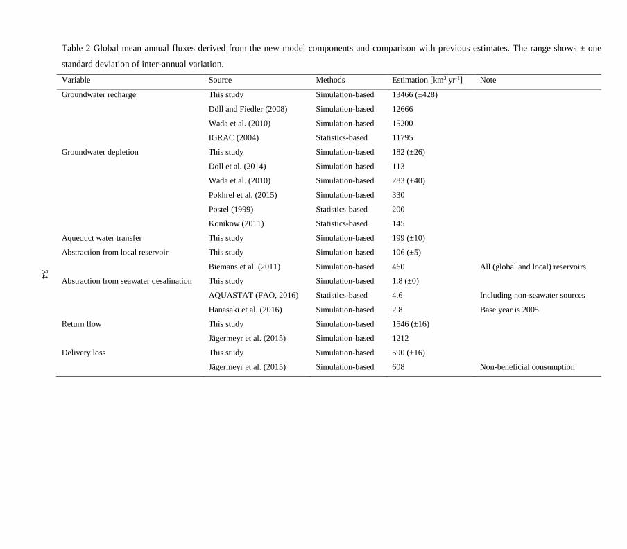
34

Table 2 Global mean annual fluxes derived from the new model components and comparison with previous estimates. The range shows ± one

standard deviation of inter-annual variation.

Variable Source Methods Estimation [km3 yr-1] Note

Groundwater recharge This study Simulation-based 13466 (±428)

Döll and Fiedler (2008) Simulation-based 12666

Wada et al. (2010) Simulation-based 15200

IGRAC (2004) Statistics-based 11795

Groundwater depletion This study Simulation-based 182 (±26)

Döll et al. (2014) Simulation-based 113

Wada et al. (2010) Simulation-based 283 (±40)

Pokhrel et al. (2015) Simulation-based 330

Postel (1999) Statistics-based 200

Konikow (2011) Statistics-based 145

Aqueduct water transfer This study Simulation-based 199 (±10)

Abstraction from local reservoir This study Simulation-based 106 (±5)

Biemans et al. (2011) Simulation-based 460 All (global and local) reservoirs

Abstraction from seawater desalination This study Simulation-based 1.8 (±0)

AQUASTAT (FAO, 2016) Statistics-based 4.6 Including non-seawater sources

Hanasaki et al. (2016) Simulation-based 2.8 Base year is 2005

Return flow This study Simulation-based 1546 (±16)

Jägermeyr et al. (2015) Simulation-based 1212

Delivery loss This study Simulation-based 590 (±16)

Jägermeyr et al. (2015) Simulation-based 608 Non-beneficial consumption

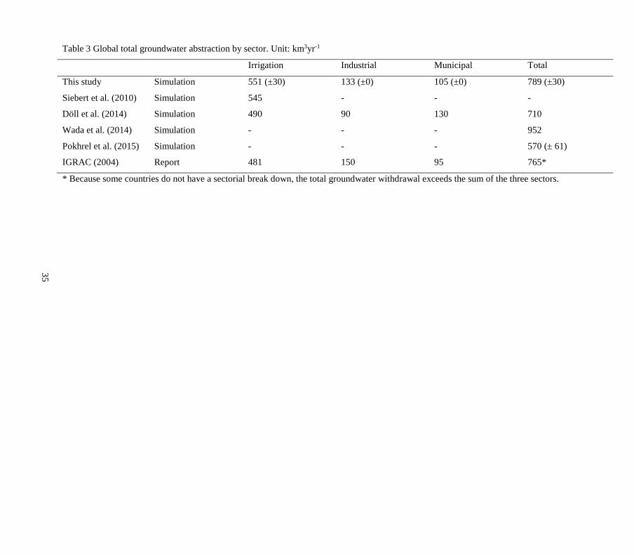
35

Table 3 Global total groundwater abstraction by sector. Unit: km3yr-1

Irrigation Industrial Municipal Total

This study Simulation 551 (±30) 133 (±0) 105 (±0) 789 (±30)

Siebert et al. (2010) Simulation 545 - - -

Döll et al. (2014) Simulation 490 90 130 710

Wada et al. (2014) Simulation - - - 952

Pokhrel et al. (2015) Simulation - - - 570 (± 61)

IGRAC (2004) Report 481 150 95 765*

* Because some countries do not have a sectorial break down, the total groundwater withdrawal exceeds the sum of the three sectors.

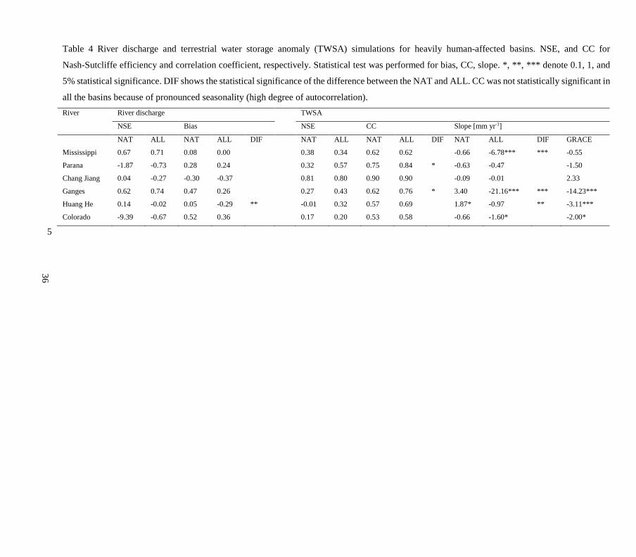
36

Table 4 River discharge and terrestrial water storage anomaly (TWSA) simulations for heavily human-affected basins. NSE, and CC for

Nash-Sutcliffe efficiency and correlation coefficient, respectively. Statistical test was performed for bias, CC, slope. *, **, *** denote 0.1, 1, and

5% statistical significance. DIF shows the statistical significance of the difference between the NAT and ALL. CC was not statistically significant in

all the basins because of pronounced seasonality (high degree of autocorrelation). River River discharge TWSA

NSE Bias NSE CC Slope [mm yr-1]

NAT ALL NAT ALL DIF NAT ALL NAT ALL DIF NAT ALL DIF GRACE

Mississippi 0.67 0.71 0.08 0.00 0.38 0.34 0.62 0.62 -0.66 -6.78*** *** -0.55

Parana -1.87 -0.73 0.28 0.24 0.32 0.57 0.75 0.84 * -0.63 -0.47 -1.50

Chang Jiang 0.04 -0.27 -0.30 -0.37 0.81 0.80 0.90 0.90 -0.09 -0.01 2.33

Ganges 0.62 0.74 0.47 0.26 0.27 0.43 0.62 0.76 * 3.40 -21.16*** *** -14.23***

Huang He 0.14 -0.02 0.05 -0.29 ** -0.01 0.32 0.57 0.69 1.87* -0.97 ** -3.11***

Colorado -9.39 -0.67 0.52 0.36 0.17 0.20 0.53 0.58 -0.66 -1.60* -2.00*

5

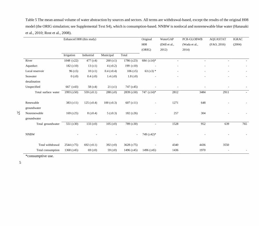
37

Table 5 The mean annual volume of water abstraction by sources and sectors. All terms are withdrawal-based, except the results of the original H08

model (the ORIG simulation; see Supplemental Text S4), which is consumption-based. NNBW is nonlocal and nonrenewable blue water (Hanasaki

et al., 2010; Rost et al., 2008). Enhanced H08 (this study) Original

H08

(ORIG)

WaterGAP

(Döll et al.,

2012)

PCR-GLOBWB

(Wada et al.,

2014)

AQUASTAT

(FAO, 2016)

IGRAC

(2004)

Irrigation Industrial Municipal Total

River 1048 (±22) 477 (±4) 260 (±1) 1786 (±23) 684 (±14)* - - - -

Aqueduct 182 (±10) 13 (±1) 4 (±0.2) 199 (±10) - - - - -

Local reservoir 96 (±5) 10 (±1) 0.4 (±0.4) 106 (±5) 63 (±3) * - - - -

Seawater

desalination

0 (±0) 0.4 (±0) 1.4 (±0) 1.8 (±0) - - - - -

Unspecified 667 (±43) 58 (±4) 21 (±1) 747 (±45) - - - - -

Total surface water 1993 (±50) 559 (±0.1) 288 (±0) 2839 (±50) 747 (±14)* 2812 3484 2911 -

Renewable

groundwater

383 (±11) 125 (±0.4) 100 (±0.3) 607 (±11) - 1271 648 - -

Nonrenewable

groundwater

169 (±25) 8 (±0.4) 5 (±0.3) 182 (±26) - 257 304 - -

Total groundwater 551 (±30) 133 (±0) 105 (±0) 789 (±30) - 1528 952 639 765

NNBW - - - - 749 (±42)* - - - -

Total withdrawal 2544 (±75) 692 (±0.1) 392 (±0) 3628 (±75) - 4340 4436 3550

Total consumption 1368 (±45) 69 (±0) 59 (±0) 1496 (±45) 1496 (±45) 1436 1970 - -

*consumptive use.

5

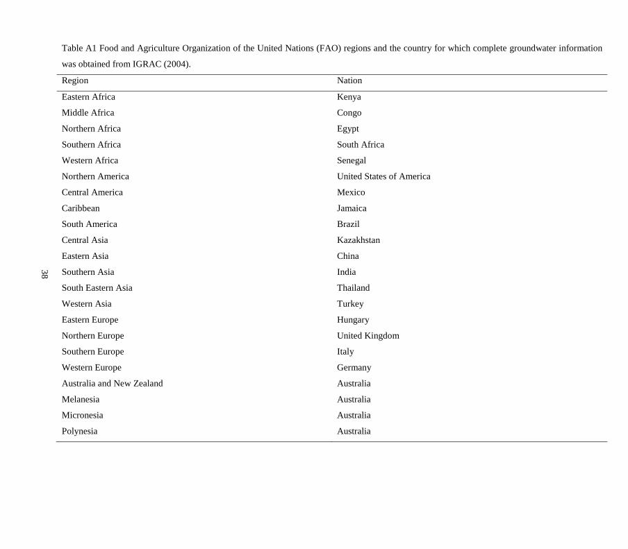
38

Table A1 Food and Agriculture Organization of the United Nations (FAO) regions and the country for which complete groundwater information

was obtained from IGRAC (2004).

Region Nation

Eastern Africa Kenya

Middle Africa Congo

Northern Africa Egypt

Southern Africa South Africa

Western Africa Senegal

Northern America United States of America

Central America Mexico

Caribbean Jamaica

South America Brazil

Central Asia Kazakhstan

Eastern Asia China

Southern Asia India

South Eastern Asia Thailand

Western Asia Turkey

Eastern Europe Hungary

Northern Europe United Kingdom

Southern Europe Italy

Western Europe Germany

Australia and New Zealand Australia

Melanesia Australia

Micronesia Australia

Polynesia Australia

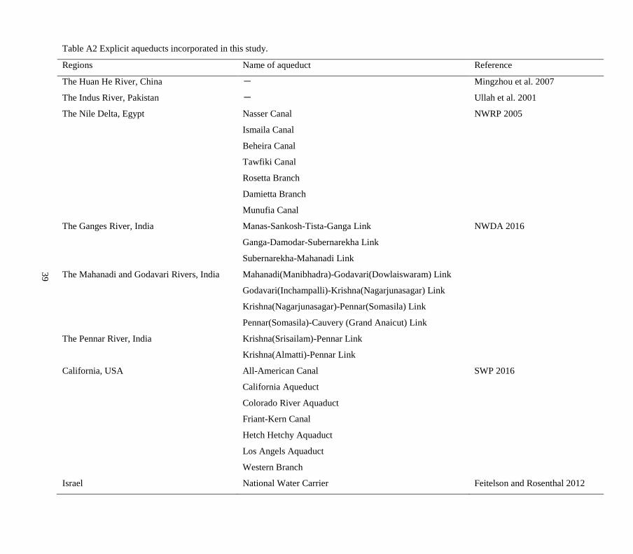
39

Table A2 Explicit aqueducts incorporated in this study.

Regions Name of aqueduct Reference

The Huan He River, China － Mingzhou et al. 2007

The Indus River, Pakistan － Ullah et al. 2001

The Nile Delta, Egypt Nasser Canal

Ismaila Canal

Beheira Canal

Tawfiki Canal

Rosetta Branch

Damietta Branch

Munufia Canal

NWRP 2005

The Ganges River, India Manas-Sankosh-Tista-Ganga Link

Ganga-Damodar-Subernarekha Link

Subernarekha-Mahanadi Link

NWDA 2016

The Mahanadi and Godavari Rivers, India Mahanadi(Manibhadra)-Godavari(Dowlaiswaram) Link

Godavari(Inchampalli)-Krishna(Nagarjunasagar) Link

Krishna(Nagarjunasagar)-Pennar(Somasila) Link

Pennar(Somasila)-Cauvery (Grand Anaicut) Link

The Pennar River, India Krishna(Srisailam)-Pennar Link

Krishna(Almatti)-Pennar Link

California, USA All-American Canal

California Aqueduct

Colorado River Aquaduct

Friant-Kern Canal

Hetch Hetchy Aquaduct

Los Angels Aquaduct

Western Branch

SWP 2016

Israel National Water Carrier Feitelson and Rosenthal 2012

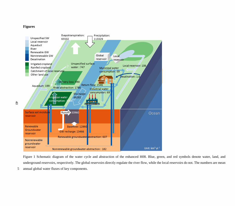
40

Figures

Figure 1 Schematic diagram of the water cycle and abstraction of the enhanced H08. Blue, green, and red symbols denote water, land, and

underground reservoirs, respectively. The global reservoirs directly regulate the river flow, while the local reservoirs do not. The numbers are mean

annual global water fluxes of key components. 5

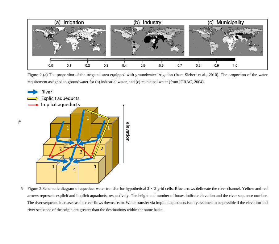
41

Figure 2 (a) The proportion of the irrigated area equipped with groundwater irrigation (from Siebert et al., 2010). The proportion of the water

requirement assigned to groundwater for (b) industrial water, and (c) municipal water (from IGRAC, 2004).

Figure 3 Schematic diagram of aqueduct water transfer for hypothetical 3 × 3 grid cells. Blue arrows delineate the river channel. Yellow and red 5

arrows represent explicit and implicit aquaducts, respectively. The height and number of boxes indicate elevation and the river sequence number.

The river sequence increases as the river flows downstream. Water transfer via implicit aqueducts is only assumed to be possible if the elevation and

river sequence of the origin are greater than the destinations within the same basin.

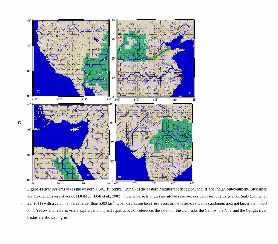
42

Figure 4 River systems of (a) the western USA, (b) central China, (c) the eastern Mediterranean region, and (d) the Indian Subcontinent. Blue lines

are the digital river network of DDM30 (Döll et al., 2002). Open inverse triangles are global reservoirs or the reservoirs listed in GRanD (Lehner et

al., 2011) with a catchment area larger than 5000 km2. Open circles are local reservoirs or the reservoirs with a catchment area not larger than 5000 5

km2. Yellow and red arrows are explicit and implicit aqueducts. For reference, the extent of the Colorado, the Yellow, the Nile, and the Ganges river

basins are shown in green.

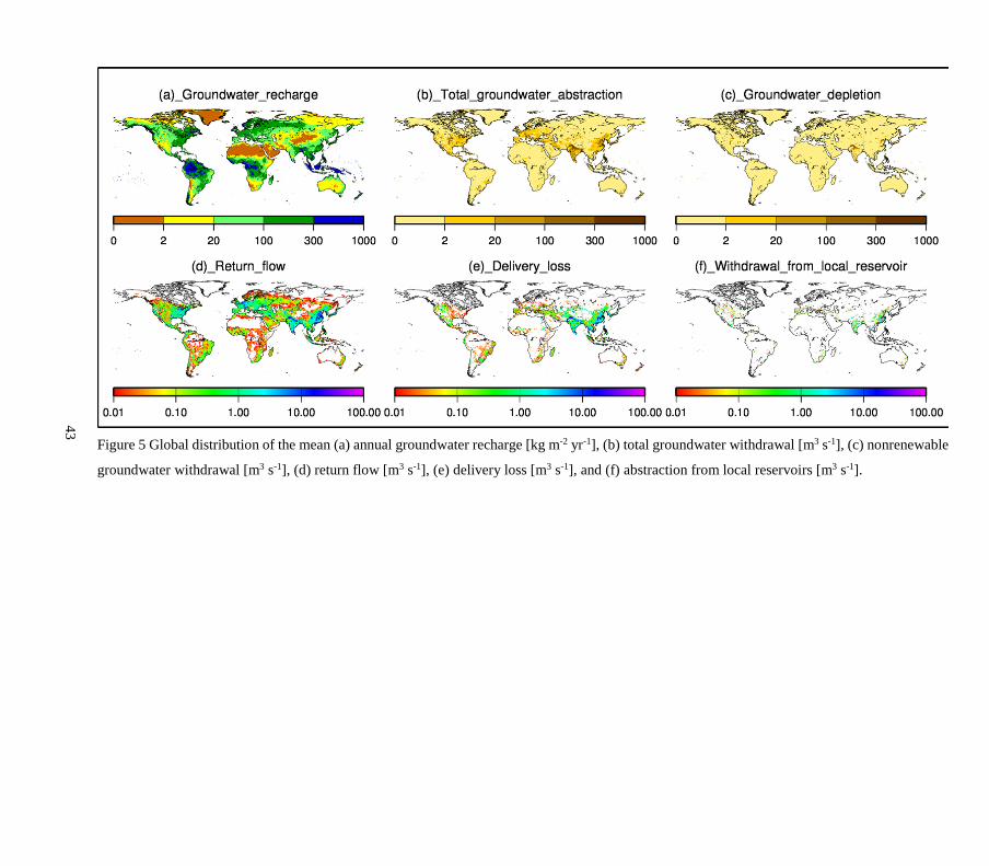
43

Figure 5 Global distribution of the mean (a) annual groundwater recharge [kg m-2 yr-1], (b) total groundwater withdrawal [m3 s-1], (c) nonrenewable

groundwater withdrawal [m3 s-1], (d) return flow [m3 s-1], (e) delivery loss [m3 s-1], and (f) abstraction from local reservoirs [m3 s-1].

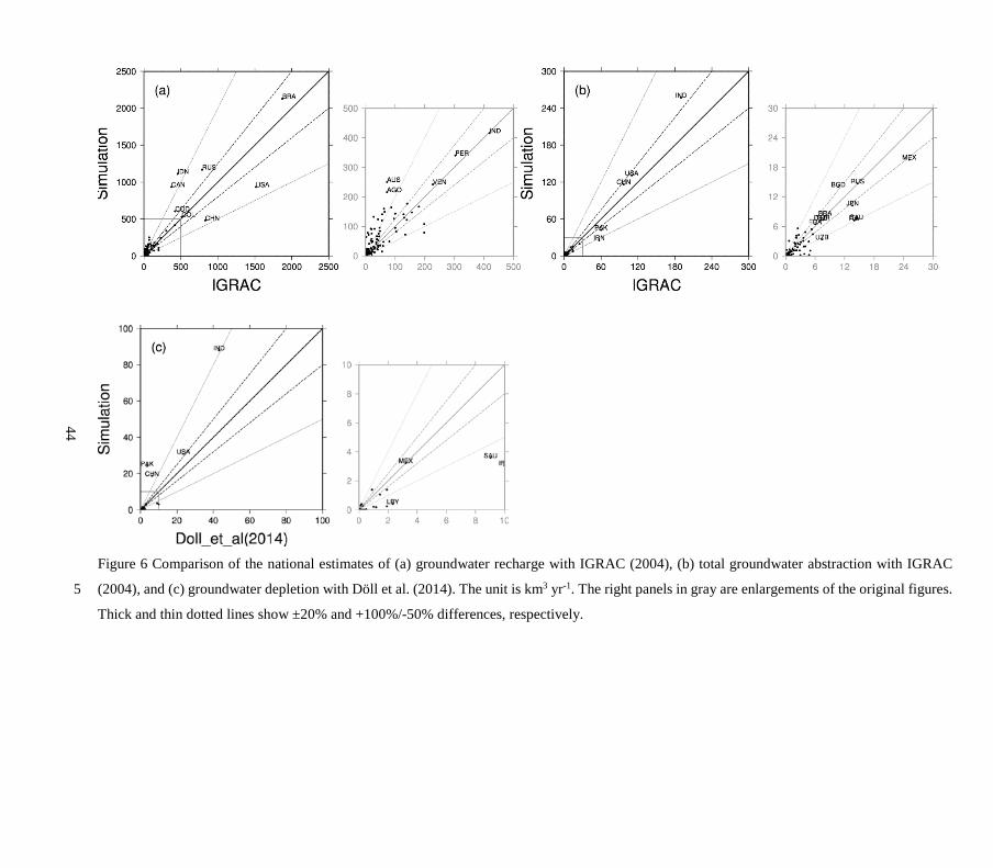
44

Figure 6 Comparison of the national estimates of (a) groundwater recharge with IGRAC (2004), (b) total groundwater abstraction with IGRAC

(2004), and (c) groundwater depletion with Döll et al. (2014). The unit is km3 yr-1. The right panels in gray are enlargements of the original figures. 5

Thick and thin dotted lines show ±20% and +100%/-50% differences, respectively.

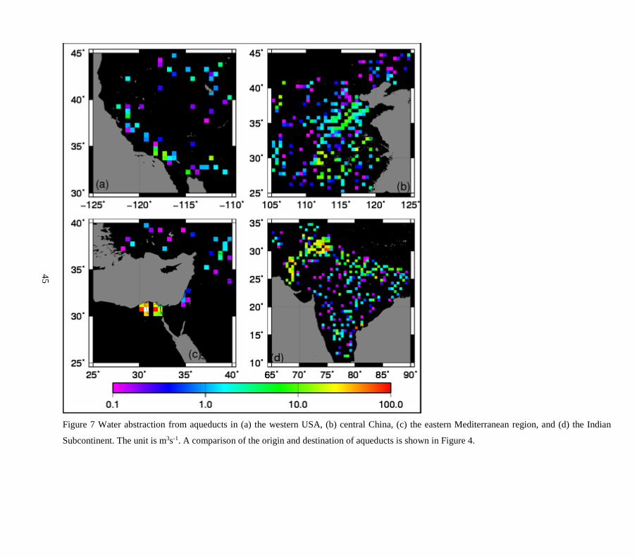
45

Figure 7 Water abstraction from aqueducts in (a) the western USA, (b) central China, (c) the eastern Mediterranean region, and (d) the Indian

Subcontinent. The unit is m3s-1. A comparison of the origin and destination of aqueducts is shown in Figure 4.

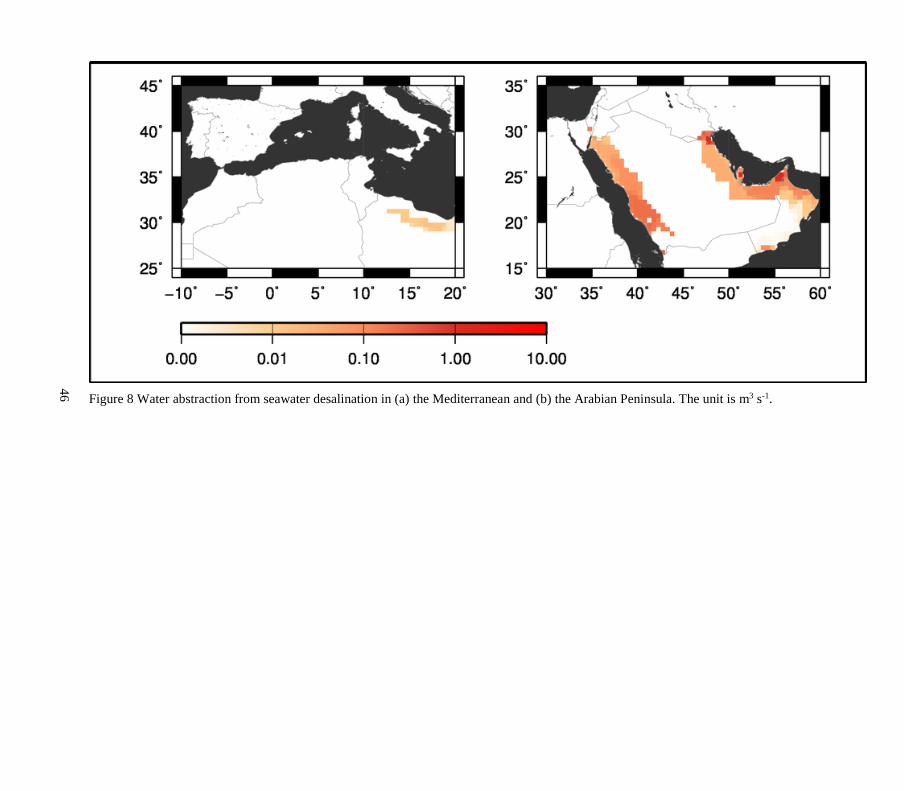
46

Figure 8 Water abstraction from seawater desalination in (a) the Mediterranean and (b) the Arabian Peninsula. The unit is m3 s-1.

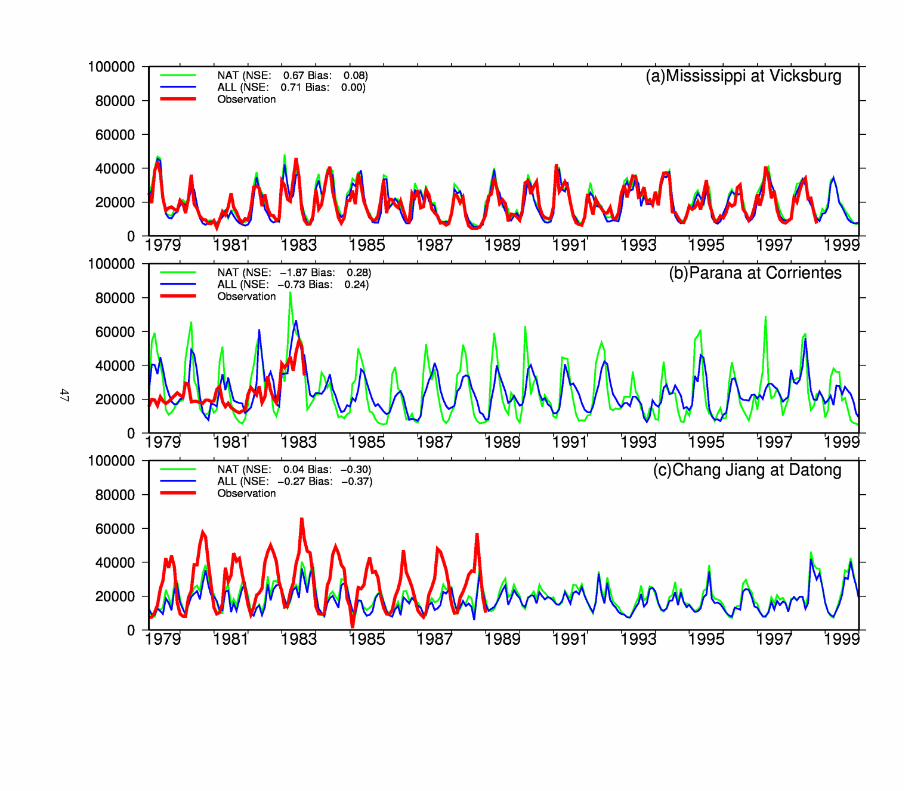
47

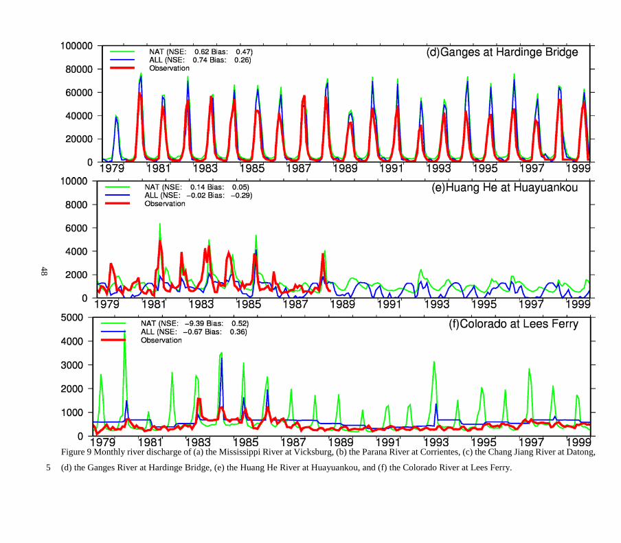
48

Figure 9 Monthly river discharge of (a) the Mississippi River at Vicksburg, (b) the Parana River at Corrientes, (c) the Chang Jiang River at Datong,

(d) the Ganges River at Hardinge Bridge, (e) the Huang He River at Huayuankou, and (f) the Colorado River at Lees Ferry. 5

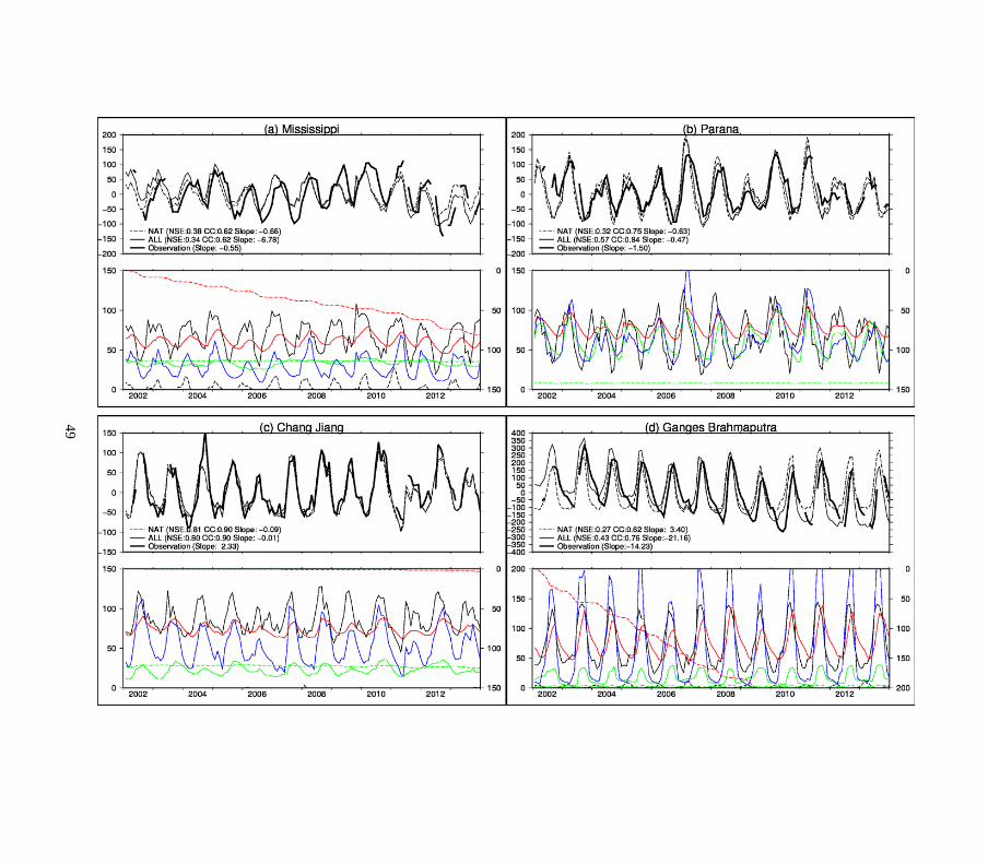
49

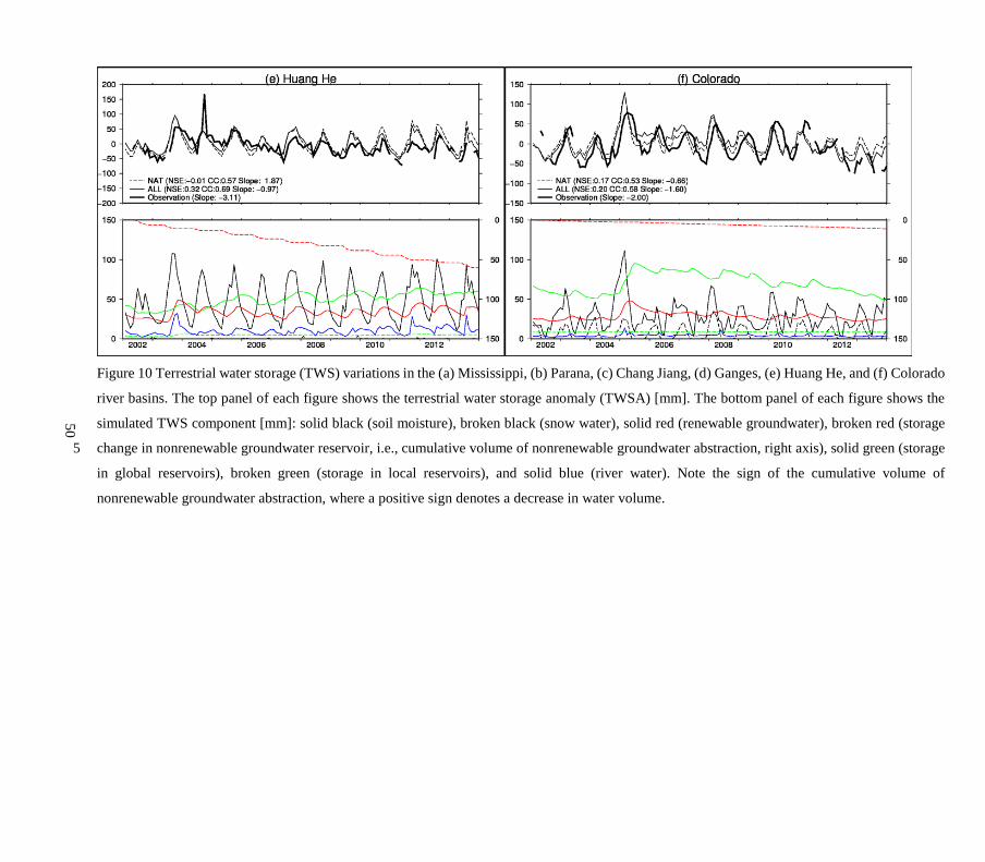
50

Figure 10 Terrestrial water storage (TWS) variations in the (a) Mississippi, (b) Parana, (c) Chang Jiang, (d) Ganges, (e) Huang He, and (f) Colorado

river basins. The top panel of each figure shows the terrestrial water storage anomaly (TWSA) [mm]. The bottom panel of each figure shows the

simulated TWS component [mm]: solid black (soil moisture), broken black (snow water), solid red (renewable groundwater), broken red (storage

change in nonrenewable groundwater reservoir, i.e., cumulative volume of nonrenewable groundwater abstraction, right axis), solid green (storage 5

in global reservoirs), broken green (storage in local reservoirs), and solid blue (river water). Note the sign of the cumulative volume of

nonrenewable groundwater abstraction, where a positive sign denotes a decrease in water volume.

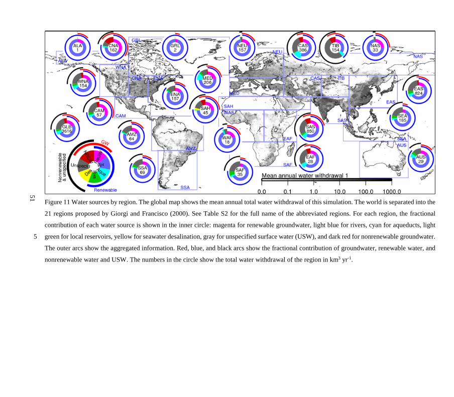
51

Figure 11 Water sources by region. The global map shows the mean annual total water withdrawal of this simulation. The world is separated into the

21 regions proposed by Giorgi and Francisco (2000). See Table S2 for the full name of the abbreviated regions. For each region, the fractional

contribution of each water source is shown in the inner circle: magenta for renewable groundwater, light blue for rivers, cyan for aqueducts, light

green for local reservoirs, yellow for seawater desalination, gray for unspecified surface water (USW), and dark red for nonrenewable groundwater. 5

The outer arcs show the aggregated information. Red, blue, and black arcs show the fractional contribution of groundwater, renewable water, and

nonrenewable water and USW. The numbers in the circle show the total water withdrawal of the region in km3 yr-1.

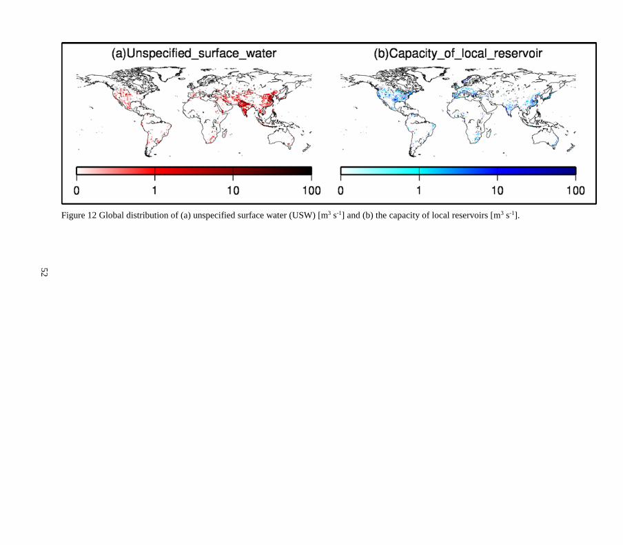
52

Figure 12 Global distribution of (a) unspecified surface water (USW) [m3 s-1] and (b) the capacity of local reservoirs [m3 s-1].

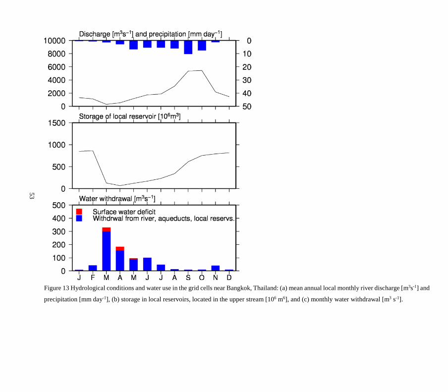
53

Figure 13 Hydrological conditions and water use in the grid cells near Bangkok, Thailand: (a) mean annual local monthly river discharge [m3s-1] and

precipitation [mm day-1], (b) storage in local reservoirs, located in the upper stream [106 m6], and (c) monthly water withdrawal [m3 s-1].

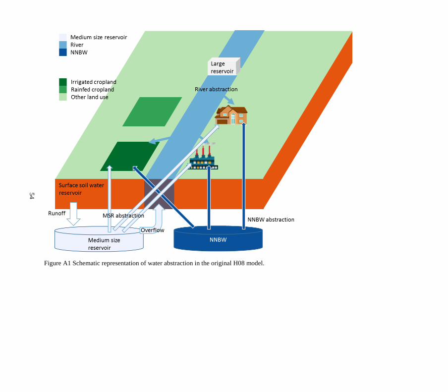
54

Figure A1 Schematic representation of water abstraction in the original H08 model.