arX

iv:2

204.

0210

7v1

[ph

ysic

s.fl

u-dy

n] 5

Apr

202

2

A GPU-accelerated computational fluid dynamics solver for

assessing shear-driven indoor airflow and virus transmission

by scale-resolved simulations

Marko Korhonena,∗, Alpo Laitinena, Gizem Ersavas Isitmana, Jose L. Jimenezb, VilleVuorinena

aDepartment of Mechanical Engineering, Aalto University, P.O. Box 14100 FI-00076 AALTO,

FinlandbDepartment of Chemistry and CIRES, University of Colorado, 216 UCB, Boulder, CO 80309-0216,

USA

Abstract

We explore the applicability of MATLAB for 3D computational fluid dynamics (CFD) ofshear-driven indoor airflows. A new scale-resolving, large-eddy simulation (LES) solvertitled DNSLABIB is proposed for MATLAB utilizing graphics processing units (GPUs).In DNSLABIB, the finite difference method is applied for the convection and diffusionterms while a Poisson equation solver based on the fast Fourier transform (FFT) is em-ployed for the pressure. The immersed boundary method (IBM) for Cartesian grids isproposed to model solid walls and objects, doorways, and air ducts by binary mask-ing of the solid/fluid domains. The solver is validated in two canonical reference cases.Then, we demonstrate the validity of DNSLABIB in a room geometry by comparing theresults against another CFD software (OpenFOAM). Next, we demonstrate the solverperformance in several isothermal indoor ventilation configurations and the implicationsof the results are discussed in the context of airborne transmission of COVID-19. Thenovel numerical findings using the new CFD solver are as follows. First, a linear scalingof DNSLABIB is demonstrated and a speed-up by a factor of 3-4 is also demonstratedin comparison to similar OpenFOAM simulations. Second, ventilation in three differ-ent indoor geometries are studied at both low (0.1m/s) and high (1m/s) airflow ratescorresponding to Re = 5000 and Re = 50000. An analysis of the indoor CO2 concen-tration is carried out as the room is emptied from stale, high CO2 content air. Weestimate the air changes per hour (ACH) values for three different room geometries andshow that the numerical estimates from 3D CFD simulations may differ by 80–150 %(Re = 50000) and 75–140 % (Re = 5000) from the theoretical ACH value based onthe perfect mixing assumption. Third, the analysis of the CO2 probability distributions(PDFs) indicates a relatively non-uniform distribution of fresh air indoors. Fourth, uti-lizing a time-dependent Wells-Riley analysis, an example is provided on the growth of thecumulative infection risk which is shown to reduce rapidly after the ventilation is started.The average infection risk is shown to reduce by a factor of 2 for lower ventilation rates(ACH=3.4-6.3) and 10 for the the higher ventilation rates (ACH=37-64). Finally, weutilize the new solver to comment on respiratory particle transport indoors. The pri-mary contribution of the paper is to provide an efficient, GPU compatible CFD solverenvironment enabling scale-resolved simulations (LES/DNS) of airflow in large indoor

1

geometries on a desktop computer. The demonstrated efficacy of MATLAB for GPUcomputing indicates a high potential of DNSLABIB for various future developments onairflow prediction.

Keywords: Computational Fluid Dynamics (CFD), COVID-19 / SARS-CoV-2, indoorventilation, air changes per hour (ACH), Wells-Riley infection model

1. Introduction

The COVID-19 pandemic has set an unprecedented demand for multidisciplinary re-search to comprehend the transmission mechanisms of the SARS-CoV-2 virus [1]. At theonset of the pandemic, the virus was initially assumed to transmit predominantly vialarger droplets and fomites present on surfaces [1]. However, since the early 2020, con-sistent and mounting evidence on the airborne transmission of the SARS-CoV-2 virushas accumulated [2–14]. Within the aerosol physics community, the suspension timeof airborne particles in air has been well-established for a century. Therefore, duringthe pandemic, the fluid physics research community has further revisited various fac-tors affecting particle transport in the air. These include the impact of particle size ontheir ability to remain airborne, the effect of relative humidity on particle shrinkage aswell as particle transport over large distances in turbulent indoor airflow [15]. Indeed,early scientific contributions on the airborne transmission of the virus were providedby the physics-based computational fluid dynamics (CFD) simulations, which addressedthe airborne transport of small particles in different indoor settings. For instance, As-cione et al. conducted a comprehensive study on the effects of various HVAC retrofittingalternatives in a university faculty which included CFD simulations on the ventilationconfigurations [16]. Zhang et al. performed CFD analysis of humidity and temperaturedistributions and ventilation performance in an indoor space using Ansys FLUENT [17].Abuhegazy et al. provided a CFD simulation of a classroom in FLUENT and a detaileddiscussion on how windows, glass barriers as well as aerosol size and source might effectthe particle trajectories [18]. Other CFD studies have considered the impact of venti-lation on the distribution of aerosols from coughing using a commercial software [19]and particle trajectories in OpenFOAM [20] as well as utilizing far-UVC lightning as avirus inactivator [21]. Furthermore, various elements impacting the spread of airborneparticles, such as ventilation, air filters and masks, have been considered in assortedCFD publications [22–28]. At present, the aerosol inhalation route is broadly acknowl-edged to be one of the key mechanisms, possibly the main mechanism, of SARS-CoV-2transmission [1, 2, 29].

From the modeling perspective, Reynolds-averaged Navier-Stokes (RANS) modelinghas been favored over scale-resolved simulations in indoor airflow simulations in the pastdespite the reduced accuracy and the evidence to its inability to capture essential tur-bulent phenomena in such flows [30, 31]. While large-eddy simulation (LES) and direct

∗Corresponding authorEmail addresses: marko.korhonen@aalto.fi (Marko Korhonen), alpo.laitinen@aalto.fi (Alpo

Laitinen), gizem.ersavasisitman@aalto.fi (Gizem Ersavas Isitman), jose.jimenez@Colorado.EDU(Jose L. Jimenez), ville.vuorinen@aalto.fi (Ville Vuorinen)

Preprint submitted to Elsevier April 6, 2022

numerical simulation (DNS) can certainly mitigate these problems, these methods natu-rally imply more computational effort due to increased mesh sizes and level of complexity.In order to promote such scale-resolving approaches in realistic indoor airflow modeling,efficient computational approaches are therefore required.

In this context, the advances in GPU based computing may prove increasingly ben-eficial for these large simulations, since their architecture is well suited for performingparallel computations on large numerical systems [32] and their value specifically for CFDhas also been established [33, 34]. In addition to incompressible Navier-Stokes solvers [35–38], successful GPU implementations have been produced for multiphase flows [39–41],direct numerical simulations [42–44] and reactive flows [45, 46], for instance. Of the mostrecent work, GPU enabled CFD simulations based on the concept of artificial compress-ibility method has been demonstrated in PyFr [47–49], which has been since augmentedwith optimal Runge-Kutta schemes [50] and locally adaptive pseudo-time stepping [51]for increased performance. Additionally, in [52], a modified Chorin-Temam projectionmethod was implemented with spectral methods and utilized in solving the Navier-Stokesequations in a periodic flow geometry on a CPU in 2D. During the pandemic, the code(DNSLAB) by Vuorinen et al. [52] was extended by the authors to 3D and renderedcompatible with GPUs for periodic flows without walls. The multidisciplinary researchconsortium work by Vuorinen et al. in the spring of 2020 was among the first systematicCFD assessments of COVID-19 airborne transmission [22]. These investigations, usingseveral open-source CFD codes, implied that the DNSLAB runs on a GPU clearly out-performed OpenFOAM simulations on a supercomputer in terms of computational timefor simple problem types, i.e. fully periodic flows.

While the computational capabilities of GPUs for CFD have certainly been recog-nized by many, the inherent power of these devices can be offset by the steeply increas-ing requirement for technical expertise as the efficient implementation of the system ofequations generally involves a suitable API, such as CUDA [53]. Therefore, a more sim-plified software environment for these GPU implementations, such as MATLAB, wouldbe preferable for the majority of users. Indeed, MATLAB has been endorsed in manyother fields of scientific computing, including neuroscience [54, 55], modeling of electricalcircuits and systems [56–58] and control and communication systems [59–62]. However,similar adoption of the software in the CFD community has not been materialized andas a result, its increasing potential as an accessible computational tool may therefore beneglected. In our view, a streamlined LES simulation software with the capacity to solvevery large systems rapidly in MATLAB is therefore warranted.

Hence, in an effort to bridge the research gap, we present a GPU compatible CFDsolver for shear-driven airflow problems in simplified geometries. In our software, ease ofuse and performance are emphasized to allow scale-resolved turbulent flow simulations(similar to LES and DNS) in typical indoor environments involving ventilation airflow,for instance. The main objectives of the paper are as follows. First, to explore thepossibility of performing incompressible 3D scale-resolved flow simulations on a GPUin MATLAB. Second, to implement and validate a simplified immersed boundary (IB)method in MATLAB in order to explore indoor settings with solid obstacles, walls, tablesand furniture. Third, to employ the new solver to characterize indoor airflow for threedifferent ventilation configurations and discuss the findings in the context of airbornetransmission of COVID-19.

The paper is organized as follows: first, we introduce the underlying system of equa-3

tions, the IB method, the concept of mask functions and sources/sinks as well as thedefinition of hard walls in this context. Next, we present 2 canonical reference cases forvalidating the code. Then, the performance of the newly developed DNSLABIB codeis demonstrated in 1) the ventilation-induced emptying of a room of stale air, utilizingvarious ventilation setups, and 2) the emission of exhaled aerosols from respiratory ac-tivities such as speaking. Finally, we reiterate the main results and insights obtained inthese simulations in light of the airborne infection risk.

2. Theory and methods

2.1. Theoretical and numerical framework

In the present work the focus is on low-speed, isothermal gas flows which can bemodeled using the incompressible Navier-Stokes equations. Additionally, we study thetransport of a passive scalar field representing the indoor CO2 concentration. At theend of the paper, the airborne trajectories of a small number of Lagrangian particles isalso studied assuming one-way coupling. The pressure-velocity coupling is based on theprojection method [63], where the time integration is carried out using a 4th order explicitRunge-Kutta scheme. Additionally, the spatial derivatives in the momentum equation arediscretized using 2nd order central differences in the skew-symmetric, energy conservativeform (see e.g. [64]). In the projection step, the pressure equation is solved in the Fourierspace using the highly efficient fast Fourier transform (fft) method in MATLAB. Thefft method is considered to be a key enabler for large scale CFD simulation in Matlabalthough it restricts the simulations to fully Cartesian, equispaced grids. The projectionstep is executed only once per time step in order to speed up the code. Based on ourexperience, this approximation has a negligible influence on the actual numerical solution.

The governing equations for the fluid read

∇ · u = 0, (1)

∂u

∂t+∇ · (uu) = −∇p+ ν∇2u+ S(x, y, z) ·

uset − u

τf+ b (2)

∂c

∂t+∇ · (uc) = αc∇ · [β(x, y, z)∇c] + S(x, y, z) ·

cset − c

τf(3)

c|β=0 = 0, u|β=0 = 0,∂c

∂n |β=0= 0, (4)

where u is the velocity, p is the pressure divided by the fluid density ρ, ν is the kinematicviscosity, b is a body force, c is the passive concentration field and αc is the diffusivity ofthe concentration. The binary mask function β is used to mark the fluid phase (β = 1)and the solid phase (β = 0) respectively. On the no-slip walls, velocities are simplymultiplied by β.

In Eqs. (1) and (2), two additional terms appear: S(x, y, z) (uset − u) /τf , and b. Thelatter term is a simple body force which is needed for pressure driven flows. The former isa forcing term adjusting the velocity to a target value at the flow inlets such as windowsand ventilation ducts etc. This approach is needed since the present solver is periodic incontrast to non-periodic cases where the Dirichlet/Neumann boundary conditions for uand p can be provided as usual. In brief, the term S(x, y, z) (uset − u) /τf is formulated

4

Figure 1: In the demonstration above, a window is located at a wall (left) and air is entering throughthe window. A plane, spanned by the blue lines, displays the inflow velocity field, constrained in placewith the mask S(x, y, z) (middle). Furthermore, the mask along the red line in the left-hand-side figureis plotted on the right.

in order to establish the desired velocity uset within the relaxation time scale τf . Bysetting S(x, y, z) = 1 at the specific location, where the velocity must reach the valueuset and S(x, y, z) = 0 otherwise, the coordinate dependent mask function S(x, y, z)geometrically confines the momentum source to the targeted region of the geometry.A respective source term is also utilized in the scalar equation in order to investigatemixing.

A general mask function based on the hyperbolic tangent function is illustrated inFig. 1 and reads

S(x, y, x) =1

2

(

1− tanh(Bx

[

|x− xc|

Wx/2−

Wx/2

|x− xc|

]

)

)

·

1

2

(

1− tanh(By

[

|y − yc|

Wy/2−

Wy/2

|y − yc|

]

)

)

·

1

2

(

1− tanh(Bz

[

|z − zc|

Wz/2−

Wz/2

|z − zc|

]

)

)

, (5)

where xc, yc and zc are the volumetric center coordinates of the source region, whileWx, Wy and Wz are the window/inlet/ventilation duct dimensions of this region. Thisfunction obtains values in the range [0,1] and Bx,y,z defines the smoothness of the tran-sition between the two endpoints. In the example of Fig. 1, a window is located at awall (left) and an inflow of air with a constant velocity is forced with the mask function.The inflow velocity on a plane spanned by the blue lines smoothly decreases to zero atthe windows edges (middle). The behavior of the mask function along the red line showsthis continuous transition in more detail along the x-axis (right). Here, the width of thetransition region, denoted by δ, is highly dependent on the Bx parameter in Eq. (5).

Furthermore, the FFT approach in the pressure equation entails a periodic solution,which requires special consideration when creating inflow/outflow boundary conditions.In general, these can be imposed as follows in our code. Inflow through an opening (e.g.

5

Figure 2: The spectral approach employed in solving the pressure equation in this work necessitatesmaintaining periodicity in the solution. This may be achieved naturally by a suitable inflow/outflowsetup (left) or extending the fluid region beyond the system of interest (right).

window or ceiling vent) requires either 1) modeling another window on the opposite sideof the room from which the flow can exit (Fig. 2 left), or 2) extending the fluid regionaround the room so that airflow can enter and leave the room to conserve mass (Fig. 2right). While option A is used in the cross-draught cases, option B is used in the ceilingventilation case. We note that option B requires more computational resources since anextra flow passage needs to be modeled around the room.

Additionally, to model the subgrid scale effects and stabilize the flow, we utilizeexplicit filtering of the velocity and scalar fields at the end of each timestep using a 6thorder filter. The filter is defined as follows

φ = φ+Σiγxi

∂6φ

∂x6i

, (6)

where the filter coefficient is chosen so that the Nyqvist frequency is zeroed in the Fourier

space i.e. γxi=

∆x6

i

π6 . The filter resembles a standard hyperviscosity term but avoids thecross-derivatives [65].

2.2. Solution of the pressure equation in Fourier space

The pressure equation requires particular attention near the walls. In the conventionalprojection method, one obtains a u∗ from the Navier-Stokes equation without a pressuregradient and then corrects u∗ with the pressure gradient which is solved from the Poissonequation

∇ · β(x, y, z)∇p = ∇ · u∗ (7)

u = u∗ −∇p (8)

In the expression above, the mask function β is simply used to implement the Neumannboundary condition directly to the Laplacian operator ∇ · β(x, y, z)∇p. The Fourier

6

transform of this equation can not be directly determined. However, by adding andsubtracting 1 from β, one has ∇ · β(x, y, z)∇p = ∇ · (1 + β(x, y, z) − 1)∇p. Finally,the pressure equation can be recast into the following equation where the left hand sideoperator now has a well-defined Fourier transform

∆pk+1 = ∇ · (1− β(x, y, z))∇pk +∇ · u∗. (9)

We iterate equation (9) n times evaluating the right hand side of the equation by centraldifferences from the previous available value of pressure (pk) and the non-solenoidalvelocity u∗ acquired from the momentum equation. Generally, the equation convergesvery quickly and a hard-coded value n = 4 is used here. The velocity field is thencorrected as u = u∗ −∇p, utilizing the converged solution for the pressure to yield thesolenoidal field satisfying Eq. (1).

2.3. Lagrangian particles

Proceeding to Lagrangian particles, the equations of motion (EoM) read

dup

dt=

Cd

τp(uf − up) + g, (10)

τp =ρpd

2

18ρfν, (11)

Rep =|uf − up|d

ν, (12)

Cd = 1 +1

6Re2/3p , (13)

where Rep is the particle Reynolds number, τp is the particle settling time scale, describ-ing the delay of the particle in adjusting to altered flow conditions, and Cd refers to thedrag coefficient of a particle. The subscripts p and f indicate particle and fluid proper-ties, respectively, g is the gravitational force, d is the particle radius and ρ is the (bulk)density. These equations describe the trajectory of a particle which experiences the effectof gravity as well as the drag imposed by the surrounding fluid. Since the particle re-laxation time scale τp is generally small for particles of interest here (micrometer scale),the particle equations of motion are solved using the implicit Euler method, enablinglarger time steps. Two key quantities from the EoM above are the particle terminalvelocity v∗ = gτp as well as the particle sedimentation time from height h expressed asτs = h/v∗. For h = 1.5 m and d=5/10/30 µm solid particles τs is approximately 36/9/1min respectively if the ambient airflow is non-existent. In practice this simple analysis(see e.g. [22]) indicates that particles with sizes up to 100 µm can traverse significantdistances and thus they pose a risk of also being inhaled. We further address this aspectat the end of this paper.

2.4. Overview of the DNSLABIB code

As stated earlier, we implement a numerical code to solve the governing equations (2), (3)and (9) using the MATLAB language. Accordingly, no code compilation nor external de-pendencies are required and the supported platforms currently include Windows, Linuxand macOS. Our open-source code is freely available and the structure of the program

7

Figure 3: A flow chart illustrating the code execution pipeline.

is illustrated in Fig. 3. The user initializes a case and controls the subsequent simula-tion principally via the "SetParameters.m", "CreateFields.m", "CreateGeometry.m","CreateSourceMasks.m" and "InitializeDrops.m" scripts. In "SetParameters.m",the user provides the necessary information regarding the simulation geometry, fluid prop-erties and data outputting. Importantly, the user also specifies the maximum Courantnumber, as the implementation utilizes dynamic time stepping (in "AdjustDt.m"). In"CreateGeometry.m", the user specifies the obstacles in the flow domain by formingthe β(x, y, z) field with primitive shapes. Then, in "CreateSourceMasks.m", the userspecifies the location of the sources/sinks. The user also decides on whether the sim-ulation is run on CPUs or GPUs, leading to calls to either "CreateCpuArrays.m" or"CreateGpuArrays.m". Finally, the number, size and location of Lagrangian particles isassigned in "InitializeDrops.m", after which the simulation may be launched by run-ning "NS3dLab.m". This main simulation loop calls various other functions designed tosolve the fluid and particle equations which we introduced above. "SolveNavierStokes.m"("SolveScalar.m") implements the explicit RK4 time integration, updating the convec-tive and diffusive terms in the Navier-Stokes (passive scalar transport) equations via callsto "ContructVelocityIncrement.m" ("ContructScalarIncrement.m"). Finally, theprojection step is performed in "Project.m". In an analogous manner, "SolveDrops.m"advances the particle trajectories and velocities in time by constructing the terms in theequations of motion in "AdvanceDrops.m". Based on the settings provided by the userin "SetParameters.m" the main loop issues calls intermittently to "writeHDF5.m" tooutput simulation data. Since for large systems containing tens or hundreds of millions

8

of cells and a vast number of time steps, the fluid data may routinely reach extremesizes, and therefore, special consideration must be given to the data format. Currently,the code can be set to output the fluid data in HDF5 compliant format along with theassociated XMDF metadata file or in the MATLAB native format (.mat). Additionally,the Lagrangian particle data is outputted in raw text data. In our experience, visualiz-ing large fluid data sets in HDF5 format via external software, such as ParaView, yieldssuperior read and rendering performance to many other options available. For standardusers with more modest data outputting requirements, the flow quantities, such as thevelocity field, pressure, the passive concentration (and their respective time averages)can also be forwarded to a .mat file for quick access and analysis.

2.5. Advantages and limitations of DNSLABIB

As noted, the main objective of the paper is to develop an efficient GPU-compatiblecode in MATLAB for performing scale-resolved 3D CFD simulations. Before proceedingto results, the expected advantages and limitations of DNSLABIB should be mentioned.The expected advantages of DNSLABIB include:

• Potentially high performance, specifically for large systems, due to the GPU imple-mentation. The primary contributors to the observed performance include avoidingloops (vectorization) as well as the efficient gpuArray structure and fft functionin MATLAB

• Avoiding the use of a supercomputer.

• Ease of use in configuring and executing a case for simple geometries with solidobjects.

• Scale-resolved simulations present the opportunity to capture physical flow featuressuch as shear-driven turbulent flow, mixing, and flow recirculation zones.

In contrast, the main limitations of the present DNSLABIB implementation include:

• Local mesh refinement is presently not possible due to the incorporation of fft forthe pressure equation. The mesh resolution needs to be uniform.

• Since mesh refinement is not possible, only vents and windows with a relativelylarge diameter can be resolved (e.g. over 20 computational cells per diameter) atthe moment.

• Wall models are currently not implemented in the code and one needs to rely onconstant grid resolution even at the walls.

• The obstacles are presented as simple blocks.

• Thermal sources/sinks are not presently accounted for although they are known tobe of high importance in indoor airflow configurations.

In the present paper, the main focus is in understanding the GPU compatibility ofthe present immersed boundary approach in MATLAB. Here, wall functions are not inthe focus but, instead, we aim at resolving the shear-driven flows as well as possible

9

on uniform grids. Commonly, the absence of wall models is considered detrimental tothe solution accuracy in wall-turbulence driven, high Reynolds number flows, especiallyon coarse computational grids. Here, we carry out a sensitivity assessment on Reynoldsnumber effects and discuss the cases Re = 5000 (window airflow 0.1m/s) and Re = 50000(window airflow 1m/s) to better understand how Re affects the ventilation rate whenthe airflow velocity changes. In the present cases, near-wall air velocities are rather lowspeed on the order of ∼ 0.01− 0.1 m/s so that the length scales of the viscous wall layerscales y+ < 5 − 10 are mostly reached. For Re = 50000, 88% of the computationalcells have y+ < 10. For Re = 5000 all near-wall cells have y+ < 10 while ≈98% of thenear-wall cells have y+ < 5.

3. Results

Next, the performance of DNSLABIB is explored by introducing several simulationcases of increasing complexity. First, the code is validated in two canonical referencecases: the laminar channel flow and vortex shedding due to a rectangular body mountedinto the channel. Then, we further validate the code against a scale-resolved simulationof an indoor ventilation setup performed in OpenFOAM. A number of indoor ventilationsetups are then examined to study the removal of stale air from the room and assess theinfection risk in these configurations in the context of COVID-19.

3.1. Validation and benchmarking

3.1.1. 2D laminar flows

Property Channel Channel & Cubic obstacleChannel width (D) [m] 2π ≈ 6.28 2π ≈ 6.28

Wall width [m] 0.05 ·D ≈ 0.31 0.05 ·D ≈ 0.31x-dimension (Lx) [m] 8.8 ·D ≈ 55.3 8.8 ·D ≈ 55.3y-dimension (Ly) [m] 1.1 ·D ≈ 6.91 1.1 ·D ≈ 6.91

Obstacle edge length (h) [m] – D/6 ≈ 1.05Grid 1584 × 198 1584 × 198 / 3168 × 396Re 500 84 (at obstacle)

Table 1: The simulation parameters for the flow in a channel and vortex shedding cases.

First, a laminar channel flow driven by a pressure gradient is examined to test theIB method. The simulation parameters for this case are detailed in Tab. 1. The flow isinitialized by setting a body force (acceleration) in the x-direction b = b/ρ = (bx, 0, 0). Inthis simple channel flow, the Navier-Stokes equations imply an analytical velocity profileacross the channel U(y) = (−bx/2ν)y

2 + (bxD/2ν)y which translates to a bulk velocity

of Ub =1D

∫ D

0U(y)dy = bxD

2

12ν . Since the Reynolds number is Re = UbD/ν = bxD3/12ν2,

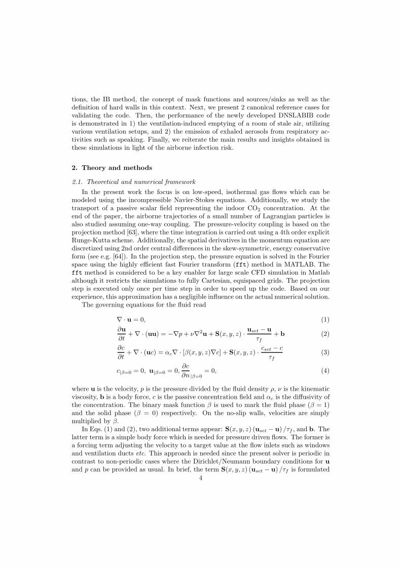
fixing the ratio bx/ν fixes the Reynolds number, which is set to Re = 500 here. As notedin Fig. 4 b), the present simple example indicates that the analytical parabolic velocityprofile is recovered in the simulation with the relative error remaining below 10−5 .

Next, as depicted in Fig. 5 a), a cube is placed at the centre line of the channel. Thepurpose of the test case is to demonstrate the performance of DNSLABIB when the wakeinteracts dynamically with the channel walls, resulting in vortex shedding. The cube is

10

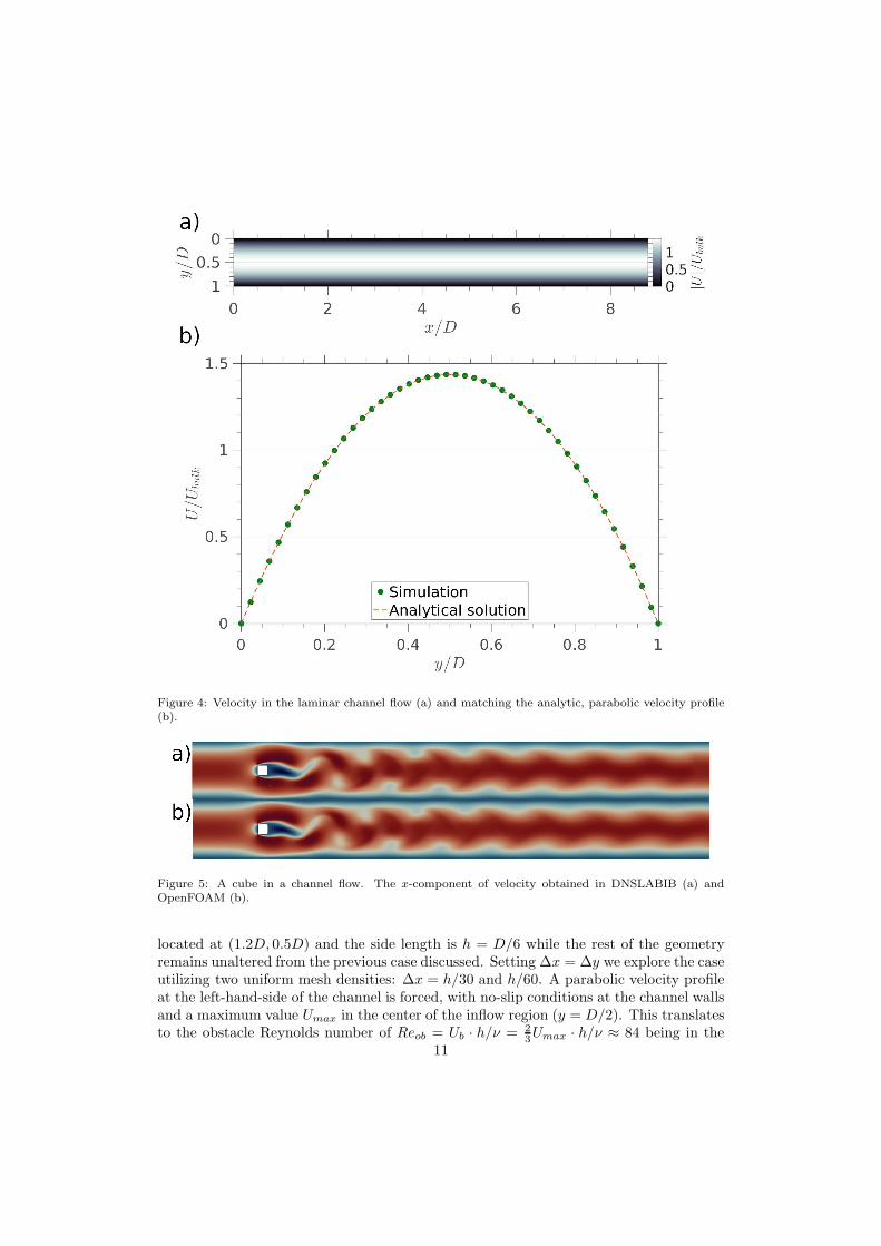
Figure 4: Velocity in the laminar channel flow (a) and matching the analytic, parabolic velocity profile(b).

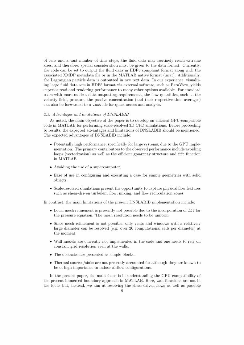
Figure 5: A cube in a channel flow. The x-component of velocity obtained in DNSLABIB (a) andOpenFOAM (b).

located at (1.2D, 0.5D) and the side length is h = D/6 while the rest of the geometryremains unaltered from the previous case discussed. Setting ∆x = ∆y we explore the caseutilizing two uniform mesh densities: ∆x = h/30 and h/60. A parabolic velocity profileat the left-hand-side of the channel is forced, with no-slip conditions at the channel wallsand a maximum value Umax in the center of the inflow region (y = D/2). This translatesto the obstacle Reynolds number of Reob = Ub · h/ν = 2

3Umax · h/ν ≈ 84 being in the

11

unsteady vortex shedding regime. The subsequent Karman vortex street is examinedin more detail in Fig. 5, where the x-component of the velocity field is examined insteady-state in both DNSLABIB (a) and OpenFOAM (b). The reference OpenFOAMsimulations are carried out with the standard incompressible PIMPLE-solver utilizing asecond order accurate backward method in time, the linear (corrected) interpolation forthe convection terms, and linear central differencing for the diffusion terms (see e.g. [66]for a similar approach). In contrast to DNSLABIB, OpenFOAM boundary conditionsare provided in a standard manner using Dirichlet/Neumann conditions.

As expected, both approaches indicate periodic vortex shedding at a distinct oscilla-tion frequency f . For the fine grid DNSLABIB simulations, the Strouhal number of theoscillation St = fh/Ub ≈ 0.2094 while the mean drag coefficient CD ≈ 3.05. The resultsare in excellent agreement with the respective values computed in OpenFOAM on thesame grid resolution with St ≈ 0.2094 and CD ≈ 3.09.

Code Cells per obstacle size Strouhal number (St) Drag coefficient (CD)DNSLABIB 30 × 30 0.2097 3.12DNSLABIB 60 × 60 0.2094 3.05OpenFOAM 30 × 30 0.192 3.21OpenFOAM 60 × 60 0.2094 3.09

Table 2: A cube in a channel flow: comparison of the Strouhal number and the drag coefficient obtainedby DNSLABIB and OpenFOAM on two different grid resolutions.

3.1.2. 3D turbulent flow indoors

In the following, airflow is simulated in a more challenging validation case at Re =5000 involving a large indoor space (8 m x 8 m x 3 m along x-, y- and z-axis, respectively)with open windows. The space is divided into two larger rooms and a corridor (3 rooms intotal) which are connected by doorways. A cross-draught is then generated as air entersand exits through the windows, ventilating the room. In addition to the Re = 5000 withwindow airflow peak velocity Uin = 0.1m/s, we also investigate a higher inflow velocity ofUin=1m/s corresponding to Re = 50000. The main validation is based on the Re = 5000case which is also rather challenging in terms of fluid dynamics while the Re = 50000case is investigated to better understand the Re sensitivity of DNSLABIB and to showthat the code stays numerically stable at extreme Reynolds numbers as well. Both ofthese cases are turbulent and hence non-trivial.

Fig. 6 illustrates the setup in more detail for Re = 50000. The Re = 5000 case wouldremain qualitatively very similar with 10× slower timescales due to the 10-fold lowervelocity scales. The midcut plane displaying the cross-section of the room is portrayedhere at z = 1.5 m. The x-component of the instantaneous velocity field is presentedcomparing DNSLABIB (a) and OpenFOAM (b) at the midcut. The panels (c) and (d)present the temporally averaged x-component of velocity for DNSLABIB and Open-FOAM respectively. Here, red color implies positive value for the velocity component,while blue suggests negative values. First, the mean velocity data in c) and d) indicatea good agreement. The key physical phenomena of the turbulent flows are marked in a)as follows. I: The shear layer generated turbulence exhibits a Kelvin-Helmholtz insta-bility a few window widths from the window (see also Fig. 10). II: Negative velocities

12

Figure 6: Instantaneous x-component of velocity at the midcut plane using DNSLABIB (a) and Open-FOAM (b). The time-averaged velocity fields obtained in DNSLABIB and OpenFOAM are visualized in(c) and (d) respectively. I Kelvin-Helmholtz instability, II recirculation zones and III flow acceleration.

and formation of recirculation zones are observed next to the walls aligned with the flowdirection. III: The flow accelerates at the more narrow doorways. These physical phe-nomena are well known and expected and it is therefore crucial that they are correctlycaptured by DNSLABIB and in qualitative agreement with the OpenFOAM code.

Fig. 7 a) details the location of three sampling lines on the midcut plane, along whichthe x-velocity component is interpolated and compared between the two computationaltools in b) for the Re = 5000 case. The comparison indicates good agreement betweenDNSLABIB and the OpenFOAM simulations. Notably, the comparison in the presentflow setup is computationally rather demanding because the flow is highly transitionaland the window width is large compared to the room dimensions so that the wallsare relatively close to the shear layers. Considering these aspects, the present resultsfor DNSLABIB at Re = 5000 can be considered to be in very good agreement withOpenFOAM. For Re = 50000, the agreement is still satisfactory. We remind that for

13

Figure 7: The time averaged x-component of velocity obtained in DNSLABIB and OpenFOAM alongthree sampling lines (b) for Re = 5000 (low ventilation rate). The sampling lines are displayed in (a)at the midcut of the simulation geometry and the arrows indicate the plotting direction (from 0 to 8m).The agreement appears very good.

the lower Reynolds number all near-wall cells have y+ < 10 while 98% of them arebelow y+ < 5. For the higher Reynolds number approximately 88% of the cells havey+ < 10. Hence, the present results provide numerical evidence that, in particular forthe Re = 5000 case, the mean velocity gradients are well resolved all the way to thewalls.

3.2. DNSLABIB performance on a GPU

Next, we discuss the simulation time for the three-room configuration emphasizingthe performance of DNSLABIB in comparison to OpenFOAM. The number of total com-putational cells for the DNSLAB case is approximately 33.3 · 106 while the OpenFOAMcase contains ∼ 16.2 · 106 cells. The DNSLABIB run for a reference room simulationtakes approximately 48 hours on a single NVIDIA Tesla A100 GPU. In contrast, theparallel OpenFOAM simulation, executed on 1040 CPU cores (Intel Xeon Gold 6230),consumes approximately 155 hours of computational time for the respective simulatedphysical time. Not only is the DNSLABIB run by a factor of 3x faster than the Open-FOAM run with almost double the computational cell count, DNSLABIB can run on amore lightweight platform containing a single GPU, avoiding using a supercomputer.

A systematic DNSLABIB scaling test for the reference room case is shown in Fig. 8detailing the computational time as a function of the mesh size as the mesh is refined. Thecomputational time is defined as the execution time of a single (NVIDIA Tesla V-100)GPU to reach a simulation time of 120 seconds (starting from t0 = 0 s). The relation-ship is linear which is an ideal result indicating no superfluous overhead is generated insimulations involving a larger number of computational cells. This result is reasonable,since the simulation data is completely contained within the VRAM of the GPU in ourbenchmark cases and thereby any degree of extraneous communication overhead shouldbe avoided.

14

Figure 8: The computational time required as a function of the system size plotted for the 3RW case atRe = 50000 (high ventilation rate). The relationship seems linear, which is ideal, indicating there is noextraneous communication overhead during the simulation. The device memory (NVIDIA Tesla V100)inhibits further benchmarking beyond N = 2 · 107.

3.3. Three indoor airflow configurations

3.3.1. Room setups and overview of the airflow

In addition to the previously validated case, Fig. 9 displays two additional ventilationsetups with the white cloud portraying the entering fresh airflow which is assumed tobe isothermal. Here, the studied rooms are empty even though simple block shapedfurniture can be easily included in DNSLABIB. Fig. 9 a) corresponds to the original3-room case while b) shows a case where the room dividers have been removed and theresulting space becomes one single open room. In panel c), the room dividers remainremoved but the ventilation airflow is now generated by vents located at the ceiling asthe windows are closed. In reality, the incoming airflow is commonly directed by gridsto enhance mixing, break strong air currents and thereby enhance the indoor airflowcomfort as well. Here, however, the inflow is simply modeled as plain air jets. Theparameters applied in these cases are detailed in Tab. 3 and in the following discussion,the cases are referred to as 3RW (3 rooms with windows), 1RW (1 room with windows)and 1RV (1 room with vents), respectively. For consistency, we have matched the inflowrate of air in these cases.

Panels d)-e) in Fig. 9 also display the instantaneous spatial patterns in the CO2

concentration field for the three setups at the midcut plane at t = 20 s for 3RW (d),1RW (e) and 1RV (f) cases respectively (Re = 50000). Here, the black (white) colordesignates areas of stale (fresh) air. For instance, in e) and f), numerous pockets ofstale air appear which remain stagnant and poorly ventilated. Some of these pockets areexpected and intuitive (room corners) while some are less intuitive such as the boundaryof the wall separating the two windows in e). The formation of stagnation zones is

15

Figure 9: Three ventilation setups with an identical airflow rate. a) Cross-draught via windows and thespace is divided to 3 smaller rooms (3RW). b) Cross-draught via windows without room-dividers (1RW).c) Vents located at the ceiling without room-dividers (1RV). d)-e) display slices of the instantaneousCO2 fields for the respective cases.

expected based on known fluid dynamics and flow recirculation near the room corners.Furthermore, turbulent airflow affects the mixing of the fresh and stale air. We notethat qualitatively very similar results are observed for the cases with Re = 5000 butthe flow simply evolves 10 times slower due to the lower window airflow velocity (notshown herein for brevity). From the viewpoint of infection risk, strong variance in theCO2 content of a room also indicates a potential spatial variance in the infection risk ofan airborne disease. While indoor CO2 measurements have recently been employed as aproxy to monitoring the virus concentration during the COVID-19 pandemic [67–70], onecould argue that the information provided by CO2 sensors can yield misleading outputif such local variances are not quantified while designing the measurement setup. Theobservations highlight the importance of accounting for the uncertainty resulting from thegeometric features of indoor spaces. Gaining a complete three dimensional description of

16

Property 1 room (windows) 3 rooms (windows) 1 room (vents)Case abbreviation 1RW 3RW 1RV

x-dimension (Lx) [m] 8 8 8y-dimension (Ly) [m] 8 8 8z-dimension (Lz) [m] 3 3 3

Grid (fine) 430 × 430 × 180 430 × 430 × 180 450 × 450 × 200Kin. viscosity [m/s2] 1.6 · 10−5 (air) 1.6 · 10−5 (air) 1.6 · 10−5 (air)

Uin/Uout [m/s] 1.0/0.1 1.0/0.1 1.0/0.1Awind [m2] 1.2 1.2 –Avent [m

2] – – 1.2Window count 4 4 –Vent count – – 4

Re 50000 / 5000 50000 / 5000 50000 / 5000

Table 3: The simulation parameters for the three room configurations for the two Reynolds numbers.

the airflow characteristics is typically only accessible via scale-resolved CFD simulations.In practice, personal CO2 meters offer real time air quality monitoring at the location ofany individual.

3.3.2. Ventilation characteristics

A commonly used engineering metric for the ventilation rate is the air changes perhour ([ACH]=1/h) defined as

ACH =V

V, (14)

where V ([V ]=m3) is the room volume and V is the volumetric airflow into the room([V ]=m3/h). In practice, ACH depends on the room airflow details, heat sources andgeometrical features. ACH value can be measured by CO2 measurements [71]. Here, weestimate ACH as follows [72]. A room is initially saturated with a relatively high CO2

content stale air (here: 1000 ppm). Then, fresh outdoor air with a low CO2 concentration(here: 400 ppm) is released into the room via windows or ventilation ducts. The meanCO2 concentration as a function of time can then be monitored to yield the ACH value.

Fig. 10 demonstrates the CO2 concentration in the 3RW simulation (Re = 50000),where the stale air is gradually displaced by clean air over time. The window jets arenoted to either impinge on the opposite wall in the back room or alternatively exit almostdirectly through the doorway to the corridor. Regions of lower ventilation performancecan emerge near wall corners within re-circulation areas (e.g. the region in close proximityof the window at lower left corner of the frame). For the 1RW case, the absence of theadditional walls imply that the window jets exit through the opposite windows withrelatively less mixing of stale and clean air.

The mean CO2 concentration can be monitored to yield the actual ACH value of eachventilation setup which differs from the theoretical ACH value. In Fig. 11, the mean CO2

content as a function of simulation time t is plotted for the studied cases. Panel a) cor-responds to simulations at Re = 50000 and b) to Re = 5000. The standard deviation isplotted as well with the error bars to indicate the uncertainty of the CO2 distributionsfor each case. Simultaneously, the analytical expression 400 · exp(−ACH · t) + 600 based

17

Figure 10: The substitution of stale air i.e. 1000 ppm CO2 concentration (black) with fresh air i.e. 400ppm CO2 concentration (white) in the 3RW case using DNSLABIB at Uin = 1m/s (Re = 50000, highventilation rate). Midcut planes of CO2 concentration at a) t = 0 s, b) t = 20 s, c) t = 60 s and d)t = 180 s.

on the ventilation theory of perfectly mixed air is displayed. The theoretical ACH coef-ficient is determined as the ratio of the flow mass fluxes involved and the room volumefor both Re = 50000 and Re = 5000 as ACH =

(

2 · 1.2m2 · 1.0m/s)

/ [8m · 8m · 3m] = 45

1/h and ACH =(

2 · 1.2m2 · 0.1m/s)

/ [8m · 8m · 3m] = 4.5 1/h, respectively. The com-putational ACH values for the various cases can be acquired by imposing a fit of the formf(t) = C0 exp(−ACHfit · t)+C1 to the data presented in Fig. 11. These values, displayedin Tab. 4, vary between 82% - 150% (Re = 50000) and 75% - 139% (Re = 5000) of thetheoretical mixing ventilation value. For Re = 50000, the displayed ACH values are high(35-70) yet the values are consistent with some of the reported values obtained in exper-imental settings involving natural ventilation [73, 74]. For Re = 5000, the ACH values(3.4-6.2) correspond to typical values observed in mechanical ventilation setups. For bothReynolds numbers, the ventilation generated by the ceiling vents (1RV) outperforms the

18

Figure 11: The time-evolution of the mean carbon dioxide content in each of the ventilated room scenariospresented earlier for the high ventilation rate, Re = 50000 (a) and the low ventilation rate, Re = 5000(b). The concentration in the room, which is initially saturated with stale air, decreases in an almostexponential manner. Clear deviations from the theoretically derived behavior is observed.

19

Simulation ACH ACHmin- ACHmax γmin ... γmax

DNSLABIB - 1RW 36.9/3.48 35.8 – 37.9 / 3.38 – 3.59 0.80 – 0.84 / 0.75 – 0.80DNSLABIB - 1RV 67.6/6.21 67.4 – 67.8 / 6.17 – 6.24 1.50 – 1.51 / 1.37 – 1.39DNSLABIB - 3RW 48.8/5.00 48.2 – 49.4 / 4.94 – 5.06 1.07 – 1.10 / 1.10 – 1.12OpenFOAM - 3RW 50.5/4.53 50.0 – 51.0 / 4.51 – 4.54 1.11 – 1.13 / 1.00 – 1.01Theoretical value 45.0 / 4.5 – –

Table 4: The ACH values estimated for Re = 5000/50000 simulations via curve fitting f(t) =C0 exp(−ACH · t) + C1 to each 〈CO2〉 displayed in Fig. 11. The last two columns detail the rangeof ACH values based on the error estimates (see Fig. 11) and their values normalized by the theoreticalACH value.

various cross-draught setups (3RW, 1RW) and among the two cross-draught simulations,the space with room dividers exhibits enhanced ventilation performance. This is due tothe improved mixing of the air masses via a combination of jet impingement, turbulenceand flow re-circulation within the back room, which were already discussed in conjunc-tion with Figs. 10 and 6. This suggests that the net impact of the solid obstacles on theACH value is more ambiguous than one might anticipate as it may depend on the exactdetails of the airflow and airflow-obstacle interactions. However, the present numericalfindings at Re = 5000 and Re = 50000 based on full 3D numerical data imply that thetheoretical ACH value may be highly inaccurate and off-set by a factor of 0.75-1.51.

In order to explore the fine structures in Fig. 10 and the CO2 profiles they entail, thedistribution of CO2 content in these cases is examined in Fig. 12, where the normalizeddistribution function f(CO2) is plotted for different instances of time, where t = 0 sdenotes the start of the simulation. The respective DNSLABIB and OpenFOAM resultsfor 3RW are displayed in a) and b) (Re = 5000) and c) and d) (Re = 50000) whilethe profiles from the 1RW and 1RV simulations obtained with DNSLABIB are plottedin c) and d) (Re = 50000). Initially, the probability distribution peaks at CO2 = 1000ppm. As the simulation and the state of ventilation progresses, the distribution veerstowards the lower end of the CO2 spectrum as anticipated. Furthermore, the distributionfunctions clearly imply non-homogeneous mixing of the air, perceived as flat and uniformdistributions, supporting the observations made earlier.

Therefore, based on the present numerical findings, we find that the airflow signifi-cantly affects the mixing patterns and dilution of the CO2 concentration in the configura-tions considered here. The routinely employed definition of ACH is limited to conditionsof perfect and extremely rapid mixing, rarely encountered in realistic indoor ventilationsetups. In reality, as exemplified by the results in Fig. 11, the standard deviation in CO2

concentration levels can be in the order of 10 − 20% of the mean value or higher, alsopointing to non-homogeneous mixing of the air masses. However, the numerical resultsindicate that the main difference between the present empty rooms stems from the flowgeometry and air supply configuration while the local variation of ACH can be relativelyimportant as well. In the presence of large pieces of furniture (e.g. book shelves) orroom dividers, the local variation of ACH may become more prominent which could beconsidered more in the future.

20

Figure 12: The distribution function f(CO2) of the carbon dioxide content at t = 200 s, t = 600 s,t = 1600 s for the 3RW case at Re = 5000 (low ventilation rate) in DNSLABIB (a) and OpenFOAM (b).Additionally, the distribution is displayed at t = 20 s, t = 60 s, t = 160 for these cases at Re = 50000(high ventilation rate) in c) and d). Finally, the profiles are also plotted for the DNSLAB simulationsof the 1RW case (e) and 1RV case (f).

3.4. Infection risk

Having extracted the ACH values from each simulation case by numerical fitting in theprevious discussion, we next proceed to the more practical implications of these resultsin terms of the infection risk. Therefore, a framework for relating the ACH and infectionrisk is required. During the COVID-19 pandemic, the classical Wells-Riley equationhas been utilized extensively for infection risk assessment [3, 75–80]. According to theWells-Riley model, the infection probability (Pinf ) can be calculated as follows

Pinf = 1− exp(−Iqpt

V), (15)

where I is the number of infectious people in the modeled setting, q is the rate ofgeneration of the infectious units termed ”quanta”, p is the respiratory rate of a person,

21

t is the exposure time and V is the air exchange rate (in units of [m3/h]). This form ofthe model assumes 1) a steady state situation reached over a longer period of time duringwhich the infectious emit virus to the air, 2) immediate and uniform mixing in the roomso that distance from the source is not taken into account, and 3) constant removal ofairborne particles by the ventilation. As a remark, under steady state conditions, theargument in the exponential function is simply the inhaled dose which is proportionalto the average concentration ([cq]=1/m3) of quanta in the room air which (I=1) can becalculated simply as follows [22]

cq =q

V=

q

ACH · V. (16)

Here, we address the infection risk in the three indoor settings, assuming that aninfectious person has occupied the space for a period of time, saturated the room withexhaled air (high CO2 content) and dispersed infectious quanta to the space which remaininfectious. Then, the infected person leaves the room, ventilation is commenced and theinfection risk for a person entering the room starts accumulating. We therefore rewritethe Wells-Riley model as follows

Pinf = 1− exp(−Q(t)), (17)

Q(t) = p

∫ t

0

cq(t) = C0p

∫ t

0

exp(−ACH · t)dt =C0p

ACH[1− exp(−ACH · t)] , (18)

where Q(t) is the effective dose a person has accumulated during time t and cq(t) isthe time-dependent average concentration of quanta in the room air. We assume thatcq is directly proportional to the previously discussed mean CO2 content, i.e. cq(t) =C0 exp(−ACH · t), where C0 represents the initial, homogeneous concentration of quantain the room saturated with stale air. This assumption considers only the small aerosolswhich remain airborne for very long periods of time (see next section).

Fig. 13 a) presents the infection risk based on Eq. (18) with the initial values of(a) 100 quanta and (b) 500 quanta homogeneously spread in the room volume, C0 ={100, 500}/(8 · 8 · 3) ≈ {0.52, 2.60} quanta/m3. In the COVID-19 context [81, 82] suchvalues could be representative to a person performing activities in an indoor setting overa 1 hour period, releasing pathogens either at a moderate (medium vocal activities, suchas talking) or very high rate (singing), respectively. The present demonstrative casesare displayed for Re = 50000 and Re = 5000 plotted with solid and transparent curvesrespectively. Furthermore, as the respiration rate of a person, the value of p = 1.2m3/h isapplied herein [22]. The key observation from panel a) is that a high enough ventilationrate reduces the average infection risk extremely efficiently.

The average infection risk approaches≈ 24% probability level if ventilation is switchedoff for the considered time window of 30 minutes compared to the probability of 0.9-1.9 %calculated for the well-ventilated cases. Even in the worst-performing ventilation setup(1RW), the infection risk reduces by a factor of 10. Similar reductions are also apparentin the results presented in panel b), where the absolute reduction in the infection risk iseven greater (≈ 80 %). For the lower ventilation rate (Re = 5000), the risk is typicallyreduced by a factor of 2 for each setup. For instance, in a), the ventilation setups at lowinflow rate reduce the infection risk from 24 % to 9-13 % and in b), from 80 % to around37-53 %. Yet, this can be considered to be a significant gain. As demonstrated herein,

22

Figure 13: The average infection risk accumulates as a function of time. Here, a scenario is illustratedwhere an infectious person has released virus to the air and a susceptible person arrives to the roomat time t = 0 s. Initial conditions (a) C0 = 100 quanta/Vroom and (b) C0 = 500 quanta/Vroom. Allconfigurations are highly effective in reducing the risk of infection at higher ventilation rates. At lowerventilation rates (transparent lines), the risk reduction is also significant.

23

window ventilation and enhancement of mechanical ventilation could be considered to bepowerful complementary tools in keeping the society open and reducing infection risksin public places such as schools, choir practices, shops and bars. As an additional note,HEPA filters deliver clean air at a certain volumetric flow rate and in analogy with ACHdefinition, an effective air change eACH (volume of filtered air / room volume) can bedefined. HEPA filters offer an energy efficient way in reducing indoor virus concentrationto increase the effective ACH value ACH∗=ACH + eACH and correspondingly lowerthe virus concentration indoors. In the future, DNSLABIB could be used to model airfiltration devices positioned at different indoor locations via the volumetric source terms.

3.5. Dispersion of airborne particles

In the previous section, we discussed the reduced infection risk associated with variousventilation setups. The estimates considered only the fraction of the airborne particleswhich are small enough so that they can be directly correlated with the indoor CO2

concentration. But what size particles are small enough to follow the airflow? During theCOVID-19 pandemic there has been a major scientific debate on the distinction betweenan aerosol and a droplet. In the aerosol community it is well understood that particlesup to sizes of 50-100 µm are able to easily remain airborne over extended times anddistances because they evaporate quickly [22]. However, until COVID-19, the medicalliterature, including WHO in their early guidance in 3/2020, adhered to an erroneous 5µm cutoff. Such an unfortunate misconception biased the early attention towards surfacetransmission which was a major error corrected later on in the pandemic when COVID-19was noted to be airborne by WHO [29]. Presently, there is a broad scientific consensus onthe airborne route as a major driver for the ongoing pandemic [5, 83]. Next, we discusshow solid particles between 1-100 µm travel in the air using DNSLABIB.

Fig. 14 presents two time snapshots of an exhaling person 0.2 seconds (a) and 0.8seconds (b) after start of exhalation. The air pulse is modelled as a particle laden jet witha diameter of D = 3 cm. The Reynolds number of the exhaled jet is Re = 7000. Thegray cloud represents the passive scalar field generated in this expulsion of air posing highCO2 concentration while the red/green/blue droplets present large (90-100 µm), medium(10-30 µm) and small (1-10 µm) particles emitted from the airways, respectively. Thesesize classes are chosen in order to comply with the clinical evidence from human expiredaerosol measurements [84]. The distribution of the particle sizes in our simulation is20% (90-100 µm), 53.3% (10-30 µm) and 26.7% (1-10 µm) of the total particle count(200), respectively. Here, particle evaporation is neglected so that the observed picturecorresponds to a conservative situation where particles sink significantly faster than theywould sink in reality e.g. at a RH=30-40% indoor relative humidity [22].

Notably, the smaller particles up to 30 µm remain airborne and they are transportedeasily through the air by the spreading air jet for considerable distances, the trajectorieshaving a clear correlation to the exhaled CO2 plume. This is consistent with our previousfindings [22] where particles of size 20 µm were shown to be transported over shelves of asupermarket between two aisles. However, the particle behavior also simply follows fromthe the particle sedimentation time in still air with τs being 36 min, 9 min and 1 min forparticle sizes of 5 µm, 10 µm and 30 µm, respectively.

Finally, Fig. 15 illustrates the aerosol emitting person placed in a room with a cross-draught and room dividers (3RW). The person emitting the infectious aerosols is locatedin the left upper corner of the room at a) t = 0 s, b) t = 20 s, c) t = 40 s and d) t = 100

24

Figure 14: Here, an exhalation is modeled as a particle laden jet. In this particular example, solid andnon-evaporating particles of size 30 µm are noted to remain airborne and easily travel horizontally toreach the airways of another person. For practical mucus droplets, evaporation shifts the critical size toa much larger value, up to 100 µm [5, 22].

s respectively. The simulations suggest that the smallest aerosols (≤ 30 µm) can rapidlytravel significant distances following the airflow, bypassing the solid walls.

The results displayed here also suggest revisiting social distancing guidelines andprotection measures in combating infectious respiratory disease. Within one minute, thetwo individuals separated from the initial aerosol source by two large walls have beenexposed to the smallest aerosols. Since the aerosols travel from room to room and furtherto the corridor, this example clearly supports the notion that in general, room dividers,plexi-glasses or visors do not provide sufficient protection from aerosols.

4. Conclusions

In the present work, we endeavored to create a CFD tool for scale-resolved simulationswith reduced computational effort. Therefore, the DNSLABIB software was programmedin the MATLAB language and implemented on a GPU. Extending the capabilities ofMATLAB to the realm of CFD, DNSLABIB provides the end-user with prior CFDexperience a starting point for further exploration.

DNSLABIB implements solid obstacles in a simplified manner via the ImmersedBoundary (IB) method and the simulations are executed on a GPU. DNSLABIB wasvalidated in two canonical reference cases, the pressure-driven channel flow and a chan-nel flow past a bluff body. The code was utilized to study three separate indoor ventila-tion configurations using scale-resolving simulations. In one of these cases, a comparisonagainst a respective OpenFOAM simulation was performed as well. A superior perfor-mance of DNSLABIB over the corresponding OpenFOAM implementation was discov-ered, the speed-up factor being in the order of 3 while avoiding usage of a supercomputerwhich is considered as a major step advocating the usage of GPUs for indoor airflowassessment.

The ventilation characteristics in the three cases were studied by monitoring the CO2

concentration as it is routinely adopted as a measured proxy for airborne transmissionrisk. The CO2 distributions and mean value over time revealed highly inhomogeneousmixing of air, contrasting the common assumption of ideally mixed air employed to

25

Figure 15: A simulation of a room with the person emitting infectious aerosols located in the top leftcorner (3RW case at Re = 50000, high ventilation rate). The a), b), c) and d) panels correspond to thesimulation times t = 0 s, t = 20 s, t = 40 s and t = 100 s, respectively after the onset of aerosol emissionby the person.

determine the ACH value. The actual ACH for each case was determined and significantdeviations from the theoretical value were noted. Collectively, the results indicatedthe presence of strong local variations in the CO2 concentration indoors. This furtheremphasizes the need to better understand the full 3D airflow features indoors usingscale-resolved simulations to ensure high air quality both locally and on average.

The extracted ACH parameters were further applied in the Wells-Riley model toassess the infection risk associated with each ventilation setup in the context of COVID-19. The provided examples indicate significantly reduced infection risk if windows areopened immediately after entering a room with stale, virus-contaminated air. However, itshould be highlighted that the actual benefits of ventilation emerge only if the inhalationdose Q remains small enough which can be achieved by 1) minimizing exposure time and2) minimizing airborne virus concentration via enhanced ventilation and/or air filtrationor masks. Even in the most conservative scenarios with the lowest ventilation rates

26

(ACH=3.4-6.3), we provided numerical examples on cases where the infection risk wasreduced by a factor of 2, which is very significant per se. For the well ventilated cases(ACH=37-67), over a 10-fold decrease in the infection risk was observed.

Finally, the transportation of respiratory particles in an exhaled jet was investigated.The studied condition resembles a case with a relative humidity of RH=100% whereparticle size reduction due to evaporation does not occur [22]. In such a conservativesetup, solid particles up to 30 µm in size were witnessed to remain airborne for prolongedperiods of time and they were therefore shown to affect observers in the consideredpremises over extended distances as well. It is clear that the traditional 5 µm cutoff issimply erroneous. However, the numerical example in question indicates that the largeparticles with sedimentation time on the order of ∼1-10 seconds will exit the exhaledair jet region quickly after which they will settle on the floor and surfaces. For largeparticles (here: 90-100µm), it is clear that the direction and strength of the exhaled andthe ambient airflow will play a major role in how well those particles may reach otherpeople’s airways near-by before settling down. The medium particles (here: 10-30 µm)are clearly able to stay airborne for a long duration of time and travel over extendeddistances. The smallest particles (here: <10 µm) are able to remain airborne for verylong periods of time. The inhalation of small and medium aerosols is the most likely routeof virus transmission as they can be unconditionally inhaled over short and long distancesand their viral content [1] as well as their number-concentration is abundant [84].

The complexity underlying the ventilation cases studied here also suggests numerousvenues for future research. A logical continuation could be the development of a wallmodel to more accurately consider boundary layers at high shear surfaces. However,as noted here in particular for Re = 5000, this aspect may not be completely criticalfor low-speed indoor airflows if most of the near-wall y+ values remain small enough.Additionally, since indoor airflow can be considerably affected by buoyancy effects, suchas heat generated by the occupants, adding an appropriate coupling (e.g. Boussinesqapproximation) between the heat sources (sinks) and the momentum equation would bereasonable as well.

Code availability

The DNSLABIB package is freely available at https://github.com/Aalto-CFD/DNSLABIB.

Acknowledgements

We thank the Academy of Finland for their financial support (grant No. 335516) andthe Aalto Science-IT project for the high-performance computational resources.

References

[1] C. C. Wang, K. A. Prather, J. Sznitman, J. L. Jimenez, S. S. Lakdawala, Z. Tufekci, L. C. Marr,Airborne transmission of respiratory viruses, Science 373 (6558) (2021) eabd9149.

[2] R. Tellier, COVID-19: the case for aerosol transmission, Interface Focus 12 (2) (2022) 20210072.[3] M. Auvinen, J. Kuula, T. Gronholm, M. Suhring, A. Hellsten, High-resolution large-eddy simula-

tion of indoor turbulence and its effect on airborne transmission of respiratory pathogens—modelvalidation and infection probability analysis, Physics of Fluids 34 (1) (2022) 015124.

27

[4] E. L. Anderson, P. Turnham, J. R. Griffin, C. C. Clarke, Consideration of the aerosol transmissionfor COVID-19 and public health, Risk Analysis 40 (5) (2020) 902–907.

[5] S. Tang, Y. Mao, R. M. Jones, Q. Tan, J. S. Ji, N. Li, J. Shen, Y. Lv, L. Pan, P. Ding, et al.,Aerosol transmission of SARS-CoV-2? evidence, prevention and control, Environment international144 (2020) 106039.

[6] M. Jayaweera, H. Perera, B. Gunawardana, J. Manatunge, Transmission of COVID-19 virus bydroplets and aerosols: A critical review on the unresolved dichotomy, Environmental research (2020)109819.

[7] R. Mittal, R. Ni, J.-H. Seo, The flow physics of COVID-19, Journal of fluid Mechanics 894 (2020).[8] A. C. Fears, W. B. Klimstra, P. Duprex, A. Hartman, S. C. Weaver, K. S. Plante, D. Mirchandani,

J. A. Plante, P. V. Aguilar, D. Fernandez, et al., Persistence of severe acute respiratory syndromecoronavirus 2 in aerosol suspensions, Emerging infectious diseases 26 (9) (2020) 2168.

[9] N. Van Doremalen, T. Bushmaker, D. H. Morris, M. G. Holbrook, A. Gamble, B. N. Williamson,A. Tamin, J. L. Harcourt, N. J. Thornburg, S. I. Gerber, et al., Aerosol and surface stability ofSARS-CoV-2 as compared with SARS-CoV-1, New England journal of medicine 382 (16) (2020)1564–1567.

[10] R. Zhang, Y. Li, A. L. Zhang, Y. Wang, M. J. Molina, Identifying airborne transmission as thedominant route for the spread of COVID-19, Proceedings of the National Academy of Sciences117 (26) (2020) 14857–14863.

[11] N. Wilson, A. Norton, F. Young, D. Collins, Airborne transmission of severe acute respiratorysyndrome coronavirus-2 to healthcare workers: a narrative review, Anaesthesia 75 (8) (2020) 1086–1095.

[12] K. J. Godri Pollitt, J. Peccia, A. I. Ko, N. Kaminski, C. S. Dela Cruz, D. W. Nebert, J. K.Reichardt, D. C. Thompson, V. Vasiliou, COVID-19 vulnerability: the potential impact of geneticsusceptibility and airborne transmission, Human genomics 14 (2020) 1–7.

[13] Y. Li, H. Qian, J. Hang, X. Chen, P. Cheng, H. Ling, S. Wang, P. Liang, J. Li, S. Xiao, et al.,Probable airborne transmission of SARS-CoV-2 in a poorly ventilated restaurant, Building andEnvironment (2021) 107788.

[14] A. Henriques, N. Mounet, L. Aleixo, P. Elson, J. Devine, G. Azzopardi, M. Andreini, M. Rognlien,N. Tarocco, J. Tang, Modelling airborne transmission of SARS-CoV-2 using CARA: risk assessmentfor enclosed spaces, Interface Focus 12 (2) (2022) 20210076.

[15] I. Eames, J.-B. Flor, Spread of infectious agents through the air in complex spaces, Interface Focus12 (2) (2022) 20210080.

[16] F. Ascione, R. F. De Masi, M. Mastellone, G. P. Vanoli, The design of safe classrooms of educationalbuildings for facing contagions and transmission of diseases: A novel approach combining audits,calibrated energy models, building performance (BPS) and computational fluid dynamic (CFD)simulations, Energy and Buildings 230 (2021) 110533.

[17] F. Zhang, Y. Ryu, Simulation study on indoor air distribution and indoor humidity distribution ofthree ventilation patterns using computational fluid dynamics, Sustainability 13 (7) (2021) 3630.

[18] M. Abuhegazy, K. Talaat, O. Anderoglu, S. V. Poroseva, Numerical investigation of aerosol trans-port in a classroom with relevance to COVID-19, Physics of Fluids 32 (10) (2020) 103311.

[19] L. Borro, L. Mazzei, M. Raponi, P. Piscitelli, A. Miani, A. Secinaro, The role of air conditioningin the diffusion of Sars-CoV-2 in indoor environments: A first computational fluid dynamic model,based on investigations performed at the vatican state children’s hospital, Environmental Research193 (2021) 110343.

[20] W. Liu, T. van Hooff, Y. An, S. Hu, C. Chen, Modeling transient particle transport in transientindoor airflow by fast fluid dynamics with the markov chain method, Building and Environment186 (2020) 107323.

[21] A. G. Buchan, L. Yang, K. D. Atkinson, Predicting airborne coronavirus inactivation by far-UVCin populated rooms using a high-fidelity coupled radiation-CFD model, Scientific reports 10 (1)(2020) 1–7.

[22] V. Vuorinen, M. Aarnio, M. Alava, V. Alopaeus, N. Atanasova, M. Auvinen, N. Balasubramanian,H. Bordbar, P. Erasto, R. Grande, et al., Modelling aerosol transport and virus exposure withnumerical simulations in relation to SARS-CoV-2 transmission by inhalation indoors, Safety Science130 (2020) 104866.

[23] J. Ren, Y. Wang, Q. Liu, Y. Liu, Numerical study of three ventilation strategies in a prefabricatedCOVID-19 inpatient ward, Building and Environment 188 (2021) 107467.

[24] T. Dbouk, D. Drikakis, On airborne virus transmission in elevators and confined spaces, Physics ofFluids 33 (1) (2021) 011905.

28

[25] C. K. Ho, Modeling airborne pathogen transport and transmission risks of SARS-CoV-2, Appliedmathematical modelling 95 (2021) 297–319.

[26] C. K. Ho, Modelling airborne transmission and ventilation impacts of a COVID-19 outbreak ina restaurant in guangzhou, china, International Journal of Computational Fluid Dynamics (2021)1–19.

[27] H. Li, K. Zhong, Z. J. Zhai, Investigating the influences of ventilation on the fate of particlesgenerated by patient and medical staff in operating room, Building and Environment 180 (2020)107038.

[28] A. Khosronejad, C. Santoni, K. Flora, Z. Zhang, S. Kang, S. Payabvash, F. Sotiropoulos, Fluiddynamics simulations show that facial masks can suppress the spread of COVID-19 in indoor envi-ronments, AIP Advances 10 (12) (2020) 125109.

[29] W. H. O. (WHO), Coronavirus disease (COVID-19): How is it transmitted?URL https://www.who.int/news-room/questions-and-answers/item/coronavirus-disease-covid-19-how-is-it-transmitted

[30] P. V. Nielsen, Fifty years of CFD for room air distribution, Building and Environment 91 (2015)78–90.

[31] B. Blocken, LES over RANS in building simulation for outdoor and indoor applications: a foregoneconclusion?, in: Building Simulation, Vol. 11, Springer, 2018, pp. 821–870.

[32] G. Pratx, L. Xing, GPU computing in medical physics: A review, Medical physics 38 (5) (2011)2685–2697.

[33] K. E. Niemeyer, C.-J. Sung, Recent progress and challenges in exploiting graphics processors incomputational fluid dynamics, The Journal of Supercomputing 67 (2) (2014) 528–564.

[34] Y. Liu, X. Liu, E. Wu, Real-time 3D fluid simulation on GPU with complex obstacles, in: 12thPacific Conference on Computer Graphics and Applications, 2004. PG 2004. Proceedings., IEEE,2004, pp. 247–256.

[35] C. E. Scheidegger, J. L. Comba, R. D. Da Cunha, Practical CFD simulations on programmablegraphics hardware using SMAC, in: Computer Graphics Forum, Vol. 24, Wiley Online Library,2005, pp. 715–728.

[36] A. F. Shinn, S. P. Vanka, Implementation of a semi-implicit pressure-based multigrid fluid flowalgorithm on a graphics processing unit, in: ASME International Mechanical Engineering Congressand Exposition, Vol. 43864, 2009, pp. 125–133.

[37] J. Thibault, I. Senocak, CUDA implementation of a Navier-Stokes solver on multi-GPU desktopplatforms for incompressible flows, in: 47th AIAA aerospace sciences meeting including the newhorizons forum and aerospace exposition, 2009, p. 758.

[38] T. Brandvik, G. Pullan, An accelerated 3D Navier–Stokes solver for flows in turbomachines, ASME.J. Turbomach. 133 (2) (2010) 021025.

[39] M. Griebel, P. Zaspel, A multi-GPU accelerated solver for the three-dimensional two-phase in-compressible Navier-Stokes equations, Computer Science-Research and Development 25 (1) (2010)65–73.

[40] P. Zaspel, M. Griebel, Solving incompressible two-phase flows on multi-GPU clusters, Computers& Fluids 80 (2013) 356–364.

[41] J. M. Kelly, E. A. Divo, A. J. Kassab, Numerical solution of the two-phase incompressible Navier–Stokes equations using a GPU-accelerated meshless method, Engineering Analysis with BoundaryElements 40 (2014) 36–49.

[42] A. Shinn, S. Vanka, W.-m. Hwu, Direct numerical simulation of turbulent flow in a square ductusing a graphics processing unit (GPU), in: 40th Fluid Dynamics Conference and Exhibit, 2010, p.5029.

[43] F. Salvadore, M. Bernardini, M. Botti, GPU accelerated flow solver for direct numerical simulationof turbulent flows, Journal of Computational Physics 235 (2013) 129–142.

[44] A. Khajeh-Saeed, J. B. Perot, Direct numerical simulation of turbulence using GPU acceleratedsupercomputers, Journal of Computational Physics 235 (2013) 241–257.

[45] Y. Shi, W. H. Green, H.-W. Wong, O. O. Oluwole, Accelerating multi-dimensional combustion sim-ulations using GPU and hybrid explicit/implicit ODE integration, Combustion and Flame 159 (7)(2012) 2388–2397.

[46] K. Spafford, J. Meredith, J. Vetter, J. Chen, R. Grout, R. Sankaran, Accelerating S3D: a GPGPUcase study, in: European Conference on Parallel Processing, Springer, 2009, pp. 122–131.

[47] F. D. Witherden, A. M. Farrington, P. E. Vincent, PyFR: An open source framework for solv-ing advection–diffusion type problems on streaming architectures using the flux reconstructionapproach, Computer Physics Communications 185 (11) (2014) 3028–3040.

[48] B. C. Vermeire, F. D. Witherden, P. E. Vincent, On the utility of GPU accelerated high-order

29

methods for unsteady flow simulations: A comparison with industry-standard tools, Journal ofComputational Physics 334 (2017) 497–521.

[49] N. A. Loppi, F. D. Witherden, A. Jameson, P. E. Vincent, A high-order cross-platform incompress-ible Navier–Stokes solver via artificial compressibility with application to a turbulent jet, ComputerPhysics Communications 233 (2018) 193–205.

[50] B. C. Vermeire, N. A. Loppi, P. E. Vincent, Optimal Runge–Kutta schemes for pseudo time-steppingwith high-order unstructured methods, Journal of Computational Physics 383 (2019) 55–71.

[51] N. A. Loppi, F. D. Witherden, A. Jameson, P. E. Vincent, Locally adaptive pseudo-time steppingfor high-order flux reconstruction, Journal of Computational Physics 399 (2019) 108913.

[52] V. Vuorinen, K. Keskinen, Dnslab: A gateway to turbulent flow simulation in matlab, ComputerPhysics Communications 203 (2016) 278–289.

[53] J. Nickolls, I. Buck, M. Garland, K. Skadron, Scalable parallel programming with cuda: Is cudathe parallel programming model that application developers have been waiting for?, Queue 6 (2)(2008) 40–53.

[54] P. Peyk, A. De Cesarei, M. Junghofer, Electromagnetoencephalography software: overview andintegration with other EEG/MEG toolboxes, Computational intelligence and neuroscience 2011(2011).

[55] D. F. Goodman, R. Brette, The brian simulator, Frontiers in neuroscience 3 (2009) 26.[56] M. Daowd, N. Omar, P. Van Den Bossche, J. Van Mierlo, Passive and active battery balancing com-

parison based on MATLAB simulation, in: 2011 IEEE Vehicle Power and Propulsion Conference,IEEE, 2011, pp. 1–7.

[57] P. Mohanty, G. Bhuvaneswari, R. Balasubramanian, N. K. Dhaliwal, MATLAB based modelingto study the performance of different MPPT techniques used for solar PV system under variousoperating conditions, Renewable and Sustainable Energy Reviews 38 (2014) 581–593.

[58] S. Alegre, J. V. Mıguez, J. Carpio, Modelling of electric and parallel-hybrid electric vehicle usingMatlab/Simulink environment and planning of charging stations through a geographic informationsystem and genetic algorithms, Renewable and Sustainable Energy Reviews 74 (2017) 1020–1027.

[59] D.-W. Gu, P. Petkov, M. M. Konstantinov, Robust control design with MATLAB®, SpringerScience & Business Media, 2005.

[60] L. Wang, Model predictive control system design and implementation using MATLAB®, SpringerScience & Business Media, 2009.

[61] J. G. Proakis, M. Salehi, G. Bauch, Contemporary communication systems using MATLAB, Cen-gage Learning, 2012.

[62] Y. S. Cho, J. Kim, W. Y. Yang, C. G. Kang, MIMO-OFDM wireless communications with MAT-LAB, John Wiley & Sons, 2010.

[63] C. Canuto, M. Y. Hussaini, A. Quarteroni, T. A. Zang, Spectral methods: evolution to complexgeometries and applications to fluid dynamics, Springer Science & Business Media, 2007.

[64] V. Vuorinen, J.-P. Keskinen, C. Duwig, B. J. Boersma, On the implementation of low-dissipativeRunge–Kutta projection methods for time dependent flows using OpenFOAM®, Computers &Fluids 93 (2014) 153–163.

[65] A. Johansen, H. Klahr, Dust diffusion in protoplanetary disks by magnetorotational turbulence,The Astrophysical Journal 634 (2) (2005) 1353.

[66] P. Peltonen, K. Saari, K. Kukko, V. Vuorinen, J. Partanen, Large-eddy simulation of local heattransfer in plate and pin fin heat exchangers confined in a pipe flow, International Journal of Heatand Mass Transfer 134 (2019) 641–655.

[67] F. Villanueva, A. Notario, B. Cabanas, P. Martın, S. Salgado, M. F. Gabriel, Assessment of CO2and aerosol (pm2. 5, pm10, ufp) concentrations during the reopening of schools in the COVID-19pandemic: The case of a metropolitan area in central-southern spain, Environmental Research 197(2021) 111092.

[68] H. Kitamura, Y. Ishigaki, T. Kuriyama, T. Moritake, CO2 concentration visualization for COVID-19 infection prevention in concert halls, Environmental and Occupational Health Practice 3 (1)(2021).

[69] I. Poza-Casado, A. Llorente-Alvarez, M. A. Padilla-Marcos, Indoor air quality in naturally ventilatedclassrooms. lessons learned from a case study in a COVID-19 scenario, Sustainability 13 (15) (2021)8446.

[70] C.-Y. Chen, P.-H. Chen, J.-K. Chen, T.-C. Su, Recommendations for ventilation of indoor spacesto reduce COVID-19 transmission, Journal of the Formosan Medical Association 120 (12) (2021)2055–2060.

30

[71] L. Schibuola, C. Tambani, High energy efficiency ventilation to limit COVID-19 contagion in schoolenvironments, Energy and Buildings 240 (2021) 110882.

[72] T. Bartzanas, C. Kittas, A. Sapounas, C. Nikita-Martzopoulou, Analysis of airflow through ex-perimental rural buildings: Sensitivity to turbulence models, Biosystems engineering 97 (2) (2007)229–239.

[73] A. R. Escombe, C. C. Oeser, R. H. Gilman, M. Navincopa, E. Ticona, W. Pan, C. Martınez,J. Chacaltana, R. Rodrıguez, D. A. J. Moore, et al., Natural ventilation for the prevention ofairborne contagion, PLoS medicine 4 (2) (2007) e68.

[74] H. Qian, Y. Li, W. Seto, P. Ching, W. Ching, H. Sun, Natural ventilation for reducing airborneinfection in hospitals, Building and Environment 45 (3) (2010) 559–565.

[75] H. Dai, B. Zhao, Association of the infection probability of COVID-19 with ventilation rates inconfined spaces, in: Building Simulation, Vol. 13, Springer, 2020, pp. 1321–1327.

[76] C. Sun, Z. Zhai, The efficacy of social distance and ventilation effectiveness in preventing COVID-19transmission, Sustainable cities and society 62 (2020) 102390.

[77] A. Foster, M. Kinzel, Estimating COVID-19 exposure in a classroom setting: A comparison betweenmathematical and numerical models, Physics of Fluids 33 (2) (2021) 021904.

[78] S. Park, Y. Choi, D. Song, E. K. Kim, Natural ventilation strategy and related issues to preventcoronavirus disease 2019 (COVID-19) airborne transmission in a school building, Science of theTotal Environment 789 (2021) 147764.

[79] Z. Peng, J. L. Jimenez, Exhaled CO2 as a COVID-19 infection risk proxy for different indoorenvironments and activities, Environmental Science & Technology Letters 8 (5) (2021) 392–397.

[80] Z. Wang, E. R. Galea, A. Grandison, J. Ewer, F. Jia, A coupled computational fluid dynamicsand Wells-Riley model to predict COVID-19 infection probability for passengers on long-distancetrains, Safety science 147 (2022) 105572.

[81] G. Buonanno, L. Stabile, L. Morawska, Estimation of airborne viral emission: Quanta emission rateof SARS-CoV-2 for infection risk assessment, Environment international 141 (2020) 105794.

[82] G. Buonanno, L. Morawska, L. Stabile, Quantitative assessment of the risk of airborne transmissionof SARS-CoV-2 infection: prospective and retrospective applications, Environment international145 (2020) 106112.

[83] T. Greenhalgh, J. L. Jimenez, K. A. Prather, Z. Tufekci, D. Fisman, R. Schooley, Ten scientificreasons in support of airborne transmission of SARS-CoV-2, The lancet 397 (10285) (2021) 1603–1605.

[84] G. Johnson, L. Morawska, Z. Ristovski, M. Hargreaves, K. Mengersen, C. Y. H. Chao, M. Wan,Y. Li, X. Xie, D. Katoshevski, et al., Modality of human expired aerosol size distributions, Journalof Aerosol Science 42 (12) (2011) 839–851.

31