Embed Size (px)
Citation preview

1
A Hebbian learning rule mediates asymmetric plasticity in aligning sensory representations. Ilana B. Witten�*, Eric I. Knudsen*, & Haim Sompolinsky** �Corresponding author: [email protected] * Neurobiology Department, Stanford University Medical Center, Stanford, CA, 94305 ** Racah Institute of Physics and Center for Neural Computation, Hebrew University, Jerusalem Israel 91904 and Center for Brain Science, Harvard University, Cambridge MA, 02138 Running head: A Hebbian learning rule mediates asymmetric plasticity
Page 1 of 46 Articles in PresS. J Neurophysiol (June 4, 2008). doi:10.1152/jn.00013.2008
Copyright © 2008 by the American Physiological Society.

2
Abstract.
In the brain, mutual spatial alignment across different sensory representations can
be shaped and maintained through plasticity. Here, we use a Hebbian model to account
for the synaptic plasticity that results from a displacement of the space representation for
one input channel relative to that of another, when the synapses from both channels are
equally plastic. Surprisingly, although the synaptic weights for the two channels obeyed
the same Hebbian learning rule, the amount of plasticity exhibited by the respective
channels was highly asymmetric and depended on the relative strength and width of the
receptive fields (RFs): the channel with the weaker or broader RFs always exhibited most
or all of the plasticity. A fundamental difference between our Hebbian model and most
previous models is that in our model synaptic weights were normalized separately for
each input channel, insuring that the circuit would respond to both sensory inputs. The
model produced three distinct regimes of plasticity dynamics (winner-take-all, mixed-
shift and no-shift), with the transition between the regimes depending on the size of the
spatial displacement and the degree of correlation between the sensory channels. In
agreement with experimental observations, plasticity was enhanced by the accumulation
of incremental adaptive adjustments to a sequence of small displacements. These same
principles would apply not only to the maintenance of spatial registry across input
channels, but also to the experience-dependent emergence of aligned representations in
developing circuits.
Keywords: Hebbian, crossmodal, learning, plasticity, computation
Introduction.
When analyzing stimuli, the central nervous system integrates information from
many different sources. The information can arise from functionally distinct channels
within the same sensory modality, such as the representations of movement and color or
the representations of the visual scene from the two eyes, or it can arise from different
sensory modalities, such as the auditory and visual representations of an object's location.
In order to integrate information appropriately, the brain must associate information from
different channels that correspond to the same object.
Page 2 of 46
3
The plasticity of convergent spatial information across channels has been studied
with various experimental manipulations. For instance, when a tadpole’s eye is rotated in
its orbit, the visual map of space in the optic tectum that originates from the rotated
ipsilateral eye reorganizes and re-aligns with the visual map of space that originates from
the contralateral eye (Udin and Grant 1999). Analogously, when barn owls are fitted with
optical displacing prisms, the auditory space map shifts to align with the displaced visual
space map (DeBello and Knudsen 2004; Knudsen 2002). When barn owls are fitted
instead with acoustic devices that alter auditory spatial cues, again the auditory space
map shifts to align with the visual space map (Gold and Knudsen 1999).
In principle, realignment of spatial representations across input channels could be
achieved either by partial adjustments in both of the representations, or by complete
adjustment of one of the representations. However, experiments show that when a
tadpole’s eye is experimentally rotated, binocular realignment is mediated predominantly
by plasticity of the inputs from the ipsilateral eye, and when a barn owl is fitted with
optical displacing prisms or acoustic devices, auditory-visual realignment is
accomplished predominantly by plasticity of the auditory inputs. Thus, in both of these
systems, plasticity appears to be highly asymmetric between the two sensory channels.
A simple explanation of these results would be that (contralateral) visual synapses
are incapable of plasticity. However, there is extensive evidence of visual plasticity
throughout the brain, including in the projection from the contralateral retina to the optic
tectum. The retinotectal synapses in the tadpole can be potentiatated or depressed,
depending on the temporal relationship between presynaptic and postsynaptic activity
(Zhang et al. 1998). Tectal neurons can rapidly develop directional sensitivity after
stimulation with moving visual stimuli (Engert et al. 2002). Additionally, in a variety of
model systems, when part of the tectum is ablated, the retinal projections compress into
the remainder of the tectum. Conversely, when part of the retina is ablated, the remaining
projections expand to fill the entire tectum (Udin and Fawcett 1988). When an additional
eye is surgically implanted in a tadpole, the projections from the implanted eye to the
optic tectum form ocular dominance columns that interdigitate with the tectal projections
from the contraletral eye (Constantine-Paton and Law 1978; Reh and Constantine-Paton
1985).
Page 3 of 46

4
Given that both input channels are capable of plasticity, the naïve expectation is
that Hebbian learning would cause both input channels to shift equally in response to a
sensory misalignment. Contrary to this expectation, we find that Hebbian learning
typically causes substantial asymmetry in the amount of plasticity across input channels
even when both channels are equally capable of plasticity. We show that small
differences in the relative strength of drive and in the relative width of the receptive fields
across input channels leads to dramatic differences in the plasticity expressed by each
input channel. Thus, relative differences in input strength and RF width across channels
can result in a dominance of one input channel over another in guiding plasticity and
could account for the development and maintenance of aligned sensory representations in
the brain.
Methods.
The architecture of our model is shown in Figure 1. For concreteness, we refer to
the two sensory input layers that converge onto the output cell as visual and auditory,
similar to the organization in the superior colliculus or optic tectum (but they could just
as well be spatiotopic representations of any two sensory parameters in any part of the
brain). Each of the presynaptic sensory layers consists of a one dimensional map of
spatially selective cells. uai and uv
i are the presynaptic firing rates of the ith cell in the
auditory and visual layers, respectively. wai describes the synaptic weight between the ith
neuron in the auditory layer and the postsynaptic cell. Similarly, wvi describes the weight
between the ith neuron in the visual layer and the postsynaptic cell. The postsynaptic
neuron has a firing rate r.
In the left column of Figure 1, the visual field was not displaced, and auditory and
visual activity arising from the same stimulus object were aligned across the two input
layers. In the right column of Figure 1, visual and auditory activity arising from the same
stimulus object was misaligned across the two input layers, as would result, for example,
from a change in eye position or optical prisms, or from a systematic misrouting of
connections during development. The projection of the visual field onto the visual layer
was displaced by 45o to the left.
Presynaptic layer
Page 4 of 46

5
Auditory and visual stimuli created Gaussian distributions of activity in the
presynaptic layers that were centered at θa(t) and θv(t), the position of the auditory and the
visual stimulus in the outside world. The ith cell in either layer fired maximally in
response to a stimulus positioned at θi in the external world. The distributions of activity
in the presynaptic layers were modeled as follows:
22
22
2/))((
2/))((
)()(
)()(vvi
aai
tvv
iv
taa
ia
eNtStu
ekNtStuσθθ
σθθ
−−
−−
=
=(1)
σa and σv represent the widths of the auditory and visual activity distributions. aN and vN
represent the normalization terms for the Gaussians such that Nztui
iv =∑ )( and
Nkztui
ia =∑ )( , where N is the number of neurons in each of the presynaptic layers and
z is a scaling factor. Thus, k denotes the ratio of the total activity in the auditory and the
visual presynaptic layers.
∑∑
=
i
iv
i
ia
tu
tuk
)(
)((2)
As derived in the Supplemental Materials, given the above constraints, the
normalization terms are
22
aa N
Nσπ
= ; 2
2
vv N
Nσπ
= (3)
The relative width of auditory and visual activity distributions is determined by
the variable b:22 / vab σσ= (4)
The binary variables Sa and Sv, which can either be 0 or 1, represent whether or
not the auditory or visual stimulus was present at a given point in time (0 corresponds to
not present; 1 corresponds to present). Assuming a probability p of the stimulus being
present at a given point in time, the average values of these variables are as follows:
<Sa(t)> = p
<Sv(t)> = p (5)
<Sa(t) Sv(t)> = fp
Page 5 of 46
6
The variable f denotes the strength of temporal correlation between the auditory
and visual presynaptic activity. If there were perfect correlation between auditory and
visual presynaptic activity, f would equal 1. In reality, f is expected to be significantly
less than 1 because most stimuli are not bimodal. If auditory and visual activity are
uncorrelated, f equals p. If the two modalities are anti-correlated, f vanishes. Since p is
likely to be much smaller than 1, we will consider here the entire range between zero and
1 as the relevant range of f.
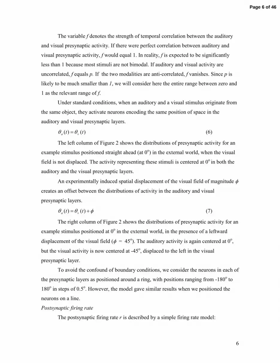
Under standard conditions, when an auditory and a visual stimulus originate from
the same object, they activate neurons encoding the same position of space in the
auditory and visual presynaptic layers.
)()( tt va θθ = (6)
The left column of Figure 2 shows the distributions of presynaptic activity for an
example stimulus positioned straight ahead (at 0o) in the external world, when the visual
field is not displaced. The activity representing these stimuli is centered at 0o in both the
auditory and the visual presynaptic layers.
An experimentally induced spatial displacement of the visual field of magnitude φ
creates an offset between the distributions of activity in the auditory and visual
presynaptic layers.
φθθ += )()( tt va (7)
The right column of Figure 2 shows the distributions of presynaptic activity for an
example stimulus positioned at 0o in the external world, in the presence of a leftward
displacement of the visual field (φ = 45o). The auditory activity is again centered at 0o,
but the visual activity is now centered at -45o, displaced to the left in the visual
presynaptic layer.
To avoid the confound of boundary conditions, we consider the neurons in each of
the presynaptic layers as positioned around a ring, with positions ranging from -180o to
180o in steps of 0.5o. However, the model gave similar results when we positioned the
neurons on a line.
Postsynaptic firing rate
The postsynaptic firing rate r is described by a simple firing rate model:
Page 6 of 46

7
)( iv
iv
i
ia
iar wuwur
dtdr ∑ ++−=τ (8)
We assume that the time scale rτ of the adjustment of the firing rate of the
postsynaptic neuron is short relative to the time scale of the sensory stimulation as well as
the modulation in a neuron’s synaptic weights, hence equation (8) reduces to
)( iv
iv
i
ia
ia wuwur ∑ += (9)
Synaptic plasticity
The synaptic weights were adjusted according to a variant of a Hebbian learning
rule.
iv
iv
iv
ia
ia
ia
Hwdt
dw
Hwdt
dw
+−=
+−=(10)
where
+
+
+−><=
+−><=
∑
∑][
][
awIruH
awIruH
j
jv
iv
iv
j
ja
ia
ia
[x]+ = max(x,0) (11)
The terms iaH and i
vH comprise several components that are summed and
thresholded above zero. The threshold serves to avoid a runaway of synaptic strengths.
However, its specific form is not crucial for our results, as we found that replacing the
threshold nonlinearity with a sigmoidal nonlinearity does not affect our central findings.
The first component of iaH and i
vH is the Hebbian correlation term, >< iaru or >< i
vru ,
the time averaged product of the firing rate for the postsynaptic neuron (r) and the ith
presynaptic neuron (uai or uv
i). The second component is a subtractive suppressive term, -
∑j
jawI or - ∑
j
jvwI , which suppresses the growth of the total synaptic weights of each
sensory modality. Finally, a constant synaptic potentiation term, a, strengthens each
synapse at each iteration and prevents the decay of all the weights to zero. The terms iaw− and i
vw− in equations (10) are local weight decay terms which guarantee the overall
stabilization of the pattern of synaptic weights.
Page 7 of 46

8
We combine equations (9), (10) and (11), taking out the weights wa and wv from
the time averaging, under the assumption that they change much more slowly in time
than the presynaptic and postsynaptic firing rates. This yields the following equations:
+
+
∑∑∑
∑∑∑
+−++−=
+−++−=
][
][
j
vj
j
aj
vaij
j
vj
vvij
vi
vi
j
aj
j
vj
avij
j
aj
aaij
ai
ai
awIwCwCwdt
dw
awIwCwCwdt
dw
(12)
The ijC terms correspond to the time averaged correlation in presynaptic activity,
tj
aia
aaij uuC >=< ; t
jv
iv
vvij uuC >=< (13)
tj
via
avij uuC >=< ; t
ja
iv
vaij uuC >=<
As derived in the Supplemental Materials, under the assumption that stimulus
positions are uniformly distributed in space, the correlations correspond to Gaussian
distributions, with amplitudes, Jaa and Jvv,
∑ −−
−−
=
j
aaaaij
aji
aji
eeJC 22
22
4/)(
4/)(
σθθ
σθθ
;∑ −−
−−
=
j
vvvvij
vji
vji
eeJC 22
22
4/)(
4/)(
σθθ
σθθ
(14)
The intramodal correlations are centered at θi = θj because a neuron’s firing rate
is always most correlated with its own firing rate (Figure 3A). This is true regardless of
the presence of a spatial displacement of the visual field. For the auditory and visual
intramodal correlations depicted in Figure 3A, the auditory correlation is broader than the
visual, reflecting the fact that, for this example, the distribution of auditory presynaptic
activity is broader than that of the visual (b = 1.5, k = 1).
Under standard conditions, the crossmodal correlation terms ( avijC and va
ijC ) are
also centered at the position θi = θj because correlated auditory and visual stimuli are
aligned in space and the visual field is not displaced (Figure 3B, solid line).
∑ −−
−−
=
j
avavij
avji
avji
eeJC 22
22
2/)(
2/)(
σθθ
σθθ
;∑ −−
−−
=
j
avvaij
avji
avji
eeJC 22
22
2/)(
2/)(
σθθ
σθθ
(15)
A displacement of the visual field causes the crossmodal terms to be offset from
θi = θj by the displacement (φ) because correlated auditory and visual activity
Page 8 of 46

9
distributions in the presynaptic layers are now misaligned (Figure 3B, dotted line and
dashed line).
∑ −−
+−−
=
j
avavij
avji
avji
eeJC 22
22
2/)(
2/)(
σθθ
σφθθ
;∑ −−
−−−
=
j
avvaij
avji
avji
eeJC 22
22
2/)(
2/)(
σθθ
σφθθ
(16)
avijC and va
ijC are offset from θi = θj in opposite directions. avijC is centered at θi =
θj -φ since an auditory neuron at position i is most correlated with a visual neuron a
distance -φ away (Figure 3B, dotted line). Conversely, vaijC is centered at θi = θj+φ since
a visual neuron at position i is most correlated with an auditory neuron a distance +φ
away (Figure 3B, dashed line).
The magnitudes of the correlations, Jaa, Jav, and Jvv, are related by k, the relative
strength of auditory and visual presynaptic activity, and f, the correlation between
auditory and visual presynaptic activity.2/ kJJ vvaa = (17)
fkJJ vvav =/
The width of the crossmodal correlation, avσ , is a function of the width of the
distributions of presynaptic activity.
222vaav σσσ += (18)
Alternate forms of the model
To test whether the results were dependent on the specific form of the synaptic
suppressive term, we introduced two alternate versions of the model. The first (“Alternate
Form A”) included a multiplicative normalization in addition to the subtractive
suppressive term. We added a multiplicative term to the model, rather than replacing our
subtractive term with a multiplicative term, because a multiplicative normalization on its
own fails to generate restricted receptive fields (Miller and MacKay 1994) . In “Alternate
Form A”, at every iteration, the value of the synaptic weights are normalized by the sum
of the weights, and multiplied by a constant c, as shown below.
∑
∑←
←
j
vj
vi
vi
j
aj
ai
ai
wcww
wcww
/
/(19)
Page 9 of 46

10
The second alternate form of the model (“Alternate Form B”) was a linear variant
of a BCM learning rule (Bienenstock et al. 1982). It involved implementing a sliding
threshold to replace the original subtractive suppressive term. We replace (11) with the
following terms:
+
+
+>><−<=
+>><−<=
])([
])([2
2
aurJrHaurJrH
ivBCM
iv
iaBCM
ia (20)
Expanding >< 2r based on (9) and (13), we get
∑∑∑ ++>=<kj
vk
avjk
aj
kj
vk
vvjk
vj
kj
ak
aajk
aj wCwwCwwCwr
,,,
2 2 (21)
This sliding threshold results in the “Alternate Form B” as follows
+
+
+++−++−=
+++−++−=
∑∑∑∑∑
∑∑∑∑∑
])2([
])2([
,,,
,,,
awCwwCwwCwJwCwCwdt
dw
awCwwCwwCwkJwCwCwdt
dw
kj
vk
avjk
aj
kj
vk
vvjk
vj
kj
ak
aajk
ajBCM
j
aj
vaij
j
vj
vvij
vi
vi
kj
vk
avjk
aj
kj
vk
vvjk
vj
kj
ak
aajk
ajBCM
j
vj
avij
j
aj
aaij
ai
ai
(22)
Additionally, to test whether the results of the model were sensitive to the form of
the nonlinearity, we developed an alternate form of the model with a different
nonlinearity. In this third alternate form of the model (“Alternate Form C”), the threshold
nonlinearity in (11) is replaced with a sigmoidal nonlinearity
)tanh(1)( xxf β+= (23)
Therefore, “Alternate Form C” takes the form
)(
)(
∑∑∑
∑∑∑
+−++−=
+−++−=
j
vj
j
aj
vaij
j
vj
vvij
vi
vi
j
aj
j
vj
avij
j
aj
aaij
ai
ai
awIwCwCfwdt
dw
awIwCwCfwdt
dw
(24)
Assessment of postsynaptic RFs
The auditory and visual RFs of the postsynaptic neuron ( )( iaF θ and )( ivF θ )
were calculated by convolving the presynaptic response to a stimulus at a given position,
iθ , with the corresponding synaptic weights.
( ) ( )ja i a a j i
jF w uθ θ θ= −∑ ; ( ) ( )j
v i v v j ij
F w uθ θ θ= −∑ (25)
Page 10 of 46

11
Numerical calculations
To update the synaptic weights, the differential equations (12) were solved
numerically in Matlab using the Euler method. Gaussian distributed noise, scaled by the
square root of the time step, was added at each iteration to simulate biological noise.
In our simulations, Jvv was fixed at 2.5, σv was fixed at 5o, and I was fixed at 100,
unless otherwise stated. The synaptic weights were initialized as Gaussian distributions
centered at 0o (amplitude of 1; width at half-max of 10o). Before the spatial displacement
of the visual field was applied, the simulation was run for 30 time points to allow the
weights to stabilize. The constant potentiation term a was set to 1. The magnitude of the
noise that was added to the weights at each time point was 0.001.
The important free parameters that were studied in this work are listed in Table 1.
Table 1- Free parameters that were studied b Relative width of auditory and visual presynaptic activity distributions
k Relative total strength of auditory and visual presynaptic activity distributions
f Strength of crossmodal correlations
φ Magnitude of spatial displacement of the visual field
Results.
The goal of this work was to understand the dynamics of the compensatory
plasticity that occurs in response to a spatial displacement of one input channel relative to
another when both channels are equally plastic. In particular, we were interested in how
plasticity divides between different input channels that converge onto a postsynaptic cell
when the input channels are spatially misaligned. For concreteness, we refer to the two
sensory input layers as visual and auditory, similar to the organization in the optic tectum.
Our paradigm for inducing synaptic plasticity in the auditory and visual channels
involved two stages. First, the synaptic weights were initialized by running the simulation
with a non-displaced visual field. Then, after the synaptic weights had stabilized, we
introduced a displacement in the visual field. The auditory and visual RFs of the
postsynaptic neuron served as the read-out of plasticity. We studied the influences of
three factors in determining the extent and dynamics of RF plasticity for each modality
(Table 1): 1) differences in the profile of presynaptic activity between the two modalities
Page 11 of 46
12
(b and k), 2) the strength of the crossmodal correlation (f), and 3) the magnitude of the
visual field displacement (φ).
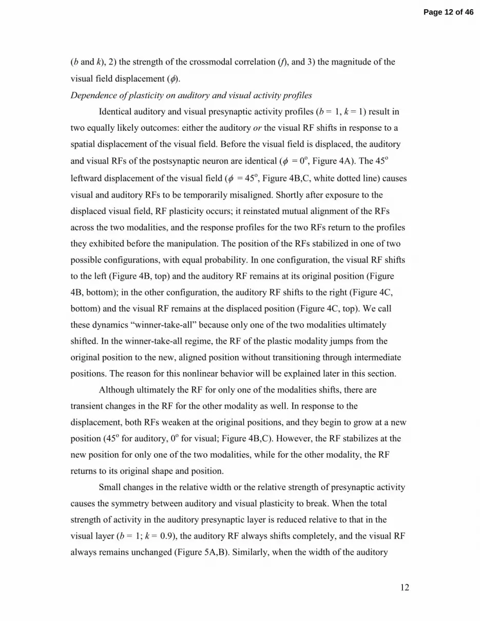
Dependence of plasticity on auditory and visual activity profiles
Identical auditory and visual presynaptic activity profiles (b = 1, k = 1) result in
two equally likely outcomes: either the auditory or the visual RF shifts in response to a
spatial displacement of the visual field. Before the visual field is displaced, the auditory
and visual RFs of the postsynaptic neuron are identical (φ = 0o, Figure 4A). The 45o
leftward displacement of the visual field (φ = 45o, Figure 4B,C, white dotted line) causes
visual and auditory RFs to be temporarily misaligned. Shortly after exposure to the
displaced visual field, RF plasticity occurs; it reinstated mutual alignment of the RFs
across the two modalities, and the response profiles for the two RFs return to the profiles
they exhibited before the manipulation. The position of the RFs stabilized in one of two
possible configurations, with equal probability. In one configuration, the visual RF shifts
to the left (Figure 4B, top) and the auditory RF remains at its original position (Figure
4B, bottom); in the other configuration, the auditory RF shifts to the right (Figure 4C,
bottom) and the visual RF remains at the displaced position (Figure 4C, top). We call
these dynamics “winner-take-all” because only one of the two modalities ultimately
shifted. In the winner-take-all regime, the RF of the plastic modality jumps from the
original position to the new, aligned position without transitioning through intermediate
positions. The reason for this nonlinear behavior will be explained later in this section.
Although ultimately the RF for only one of the modalities shifts, there are
transient changes in the RF for the other modality as well. In response to the
displacement, both RFs weaken at the original positions, and they begin to grow at a new
position (45o for auditory, 0o for visual; Figure 4B,C). However, the RF stabilizes at the
new position for only one of the two modalities, while for the other modality, the RF
returns to its original shape and position.
Small changes in the relative width or the relative strength of presynaptic activity
causes the symmetry between auditory and visual plasticity to break. When the total
strength of activity in the auditory presynaptic layer is reduced relative to that in the
visual layer (b = 1; k = 0.9), the auditory RF always shifts completely, and the visual RF
always remains unchanged (Figure 5A,B). Similarly, when the width of the auditory
Page 12 of 46

13
presynaptic activity profile is increased relative to that of the visual profile, but the total
strength of activity is the same across the modalities, the auditory RF always shifts
completely, while the visual RF remains unchanged (Figure 5C,D).
The relationship between which modality shifts and the relative width and the
relative total strength of presynaptic activity is shown in Figure 6 (black line). A good
predictor of which modality shifts is the relative strength of the mean presynaptic
weights: the modality with the weaker mean synaptic weights tends to be the modality
that shifts (Figure 6, comparison of red dotted line and black line). The mean strength of
the synaptic weights is determined by the presynaptic activity. Both decreasing the
strength of the presynaptic activity and increasing the width of the presynaptic activity
leads to a weakening of the mean synaptic weights, which in turn leads to the asymmetry
in the resulting plasticity, for reasons that are discussed below.
To gain an intuition for how auditory and visual RFs shift to compensate for the
displacement of the visual field, we must first understand the terms that drive plasticity.
The auditory and visual synaptic weights are strengthened by two correlation terms
(equation 12): the correlation of presynaptic activity within each modality (intramodal
correlation; aaijC and vv
ijC ) and the correlation of presynaptic activity across the two
modalities (crossmodal correlation; avijC and va
ijC ). The intramodal correlation strengthens
the synaptic weights without causing them to shift position in the presynaptic layer, while
the crossmodal correlation causes the weights to shift their position to compensate for the
visual field displacement. In the absence of a spatial displacement of the visual field, the
crossmodal correlation is centered at zero (Figure 3B, solid line), driving the auditory and
visual RFs to be aligned in space. In the presence of a spatial displacement of the visual
field, the crossmodal correlation terms are offset by the magnitude of the displacement
(Figure 3B, dashed and dotted lines), driving the RFs for the two modalities to separate
by the magnitude of the displacement.
The crossmodal correlation term is convolved with the visual synaptic weights
(∑j
vj
avij wC in equation 12) in order to drive auditory plasticity and is convolved with the
auditory synaptic weights to drive visual plasticity (∑j
aj
vaij wC in equation 12). Figure 7
Page 13 of 46

14
displays the distributions of synaptic weights and the convolution of the weights with the
correlation terms at several important time points in the simulation. Before the visual
field displacement, the auditory and visual weights are centered at zero (Figure 7A).
Similarly, both the intramodal correlation convolved with the appropriate weights (Figure
7D) and the crossmodal correlation convolved with the appropriate weights (Figure 7G)
are centered at zero. This is because both the intramodal and the crossmodal correlations
are centered at zero for the non-displaced visual field (Figure 3A and 3B, solid lines).
Since the weights and convolution terms are aligned, there is no force driving the
synaptic weights to shift. Immediately after the visual field displacement, there is not yet
a change in the synaptic weights and the weights are still centered at zero (Figure 7B).
The intramodal term convolved with the appropriate weights also remains unchanged
(Figure 7E). However, there is an important change in the crossmodal term convolved
with the synaptic weights. Since the crossmodal correlations are now offset from 0
(Figure 3B, dashed and dotted lines), the convolutions of the crossmodal correlations
with the weights are now offset from zero (Figure 7H). These terms now drive the
auditory weights to shift to the right and the visual weights to shift to the left. After
adaptation to the visual field displacement, the auditory weights are shifted to the right
and the visual weights remain at the original position (Figure 7C). Both the intramodal
correlations convolved with the appropriate weights (Figure 7F) and the crossmodal
correlations convolved with the appropriate weights (Figure 7I) are aligned with the
weights, so there is no term driving further changes in the distributions of the weights.
Why does the auditory, and not the visual, RF shift when the auditory presynaptic
activity is weaker or broader than the visual? When the presynaptic visual activity is
either stronger or more narrowly distributed than the auditory presynaptic activity, the
mean visual synaptic weights become stronger than the mean auditory weights (Figure 6,
red dotted line). As a result, the crossmodal term driving auditory plasticity (∑j
vj
avij wC in
equation 12; Figure 7H, blue line) becomes larger than the crossmodal term driving
visual plasticity (∑j
aj
vaij wC in equation 12; Figure 7H, red line), causing the auditory
weights to shift preferentially (Figure 7C). Notably, a narrowing of the presynaptic
activity leads to a weakening of the mean synaptic weights, even when the mean
Page 14 of 46

15
presynaptic activity is unchanged, an effect that is likely mediated by the nonlinearity
(equation 12).
Regimes with different dynamics of plasticity
So far, we have discussed winner-take-all dynamics, in which the input channel
with the weaker or broader RFs shifts by the entire visual field displacement, while the
RFs for the other input channel remains at their original position (Figure 4 and Figure 5).
Interestingly, the model produces two additional regimes with different plasticity
dynamics: a mixed-shift regime and a no-shift regime. In the mixed-shift regime (Figure
8A), the RFs of both modalities shifts and the RFs moved continuously from one position
to another (in contrast to the jump in RF position, characteristic of the winner-take-all
regime). Although both modalities shift to some extent in the mixed-shift regime, the
modality with stronger or broader input activity exhibits a greater shift (Figure 8B). The
boundary between which modality exhibits the majority of the shift is similar, but not
identical, to that in the winner-take-all regime (Figure 6). In the no-shift regime (Figure
8C), neither RF shifts, despite the displacement of the visual field, and the auditory and
visual RFs remain misaligned.
The transition between these three dynamic regimes depends primarily on two
parameters: the magnitude of the spatial displacement and the strength of the crossmodal
correlation. The magnitude of the visual field displacement (φ) affected plasticity by
determining the extent of the overlap between the crossmodal and the intramodal
correlation terms (Figure 3). As the visual field displacement increases, the overlap
decreases. The strength of the crossmodal correlations affects the dynamics because it is
the crossmodal correlations that drive plasticity. As the crossmodal correlations (f )
approach zero, the force driving plasticity approach zero as well.
The boundaries of the three regimes (winner-take-all, mixed-shift, no-shift) are
shown in Figure 9A as a function of the visual field displacement (φ) and the crossmodal
correlation (f). Understanding these boundaries requires considering the force acting on
the synaptic weights after the visual field was displaced. Immediately after a visual field
displacement, both auditory and visual synaptic weights decrease in magnitude at their
original position because they are no longer strengthened by the crossmodal correlation
term, which is shifted to a new position by the visual field displacement. This causes a
Page 15 of 46

16
decrease in the strength of the postsynaptic firing rate during the time points following
the visual field displacement (for example, see Figure 4). The decayed synaptic weights
can be estimated based on the condition in which there is no crossmodal correlation (f =
0). We calculated the force on the decayed weights (right-hand side of equation 12) and
used it to predict the regime boundaries, as described below. Notably, now we consider
the net force on the weights, incorporating the synaptic suppressive term and the
nonlinearity, whereas in Figure 7 we displayed only the contributions from the
correlation term.
The winner-take-all regime occurs when there was little overlap between the
crossmodal and the intramodal correlations (large φ) and the crossmodal correlation was
strong (large f). In this condition, the force on the synaptic weights is greater than zero for
at least one of the modalities at the aligned position of the RF (because of the large value
of f; Figure 9B, lower panel), and equal to zero for positions between the aligned position
and the initial position for both modalities (because of the large value of φ). This
distribution of the force caused the weights (for the auditory channel) to jump to the new
position, and grow rapidly through positive feedback (Figure 9B).
The no-shift regime occurrs when the crossmodal correlation (f) is small and the
spatial displacement (φ) is large relative to the crossmodal correlation. In this condition,
there is little overlap between the intramodal and the crossmodal correlations, and the
crossmodal correlation is weak. The force acting on the synaptic weights is near zero for
all positions for both modalities, so neither RF shifts (“no-shift”; Figure 9C).
The mixed-shift regime occurrs when the spatial displacement (φ) is small. In this
condition, there is substantial overlap between the crossmodal and the intramodal
correlations after the visual field displacement. This overlap creates a positive driving
force on the synaptic weights at all positions ranging from the initial to the aligned
position, so the RFs shift continuously, and both modalities shift (“mixed-shift”; Figure
9D). As shown in Figure 8A for the same parameter values, the auditory RFs shift
substantially more than the visual RFs.
After RFs shift, the RF shape recovers to that observed before plasticity (for
example, see Figure 8A). This is because both before the visual field was displaced, and
after the auditory RF shifts in response to the displaced visual field, the crossmodal
Page 16 of 46
17
correlation is aligned with the RF, so the force driving the synaptic weights is identical
(equation 12). However, when the RF does not shift in response to a displaced visual
field (“no-shift”; Figure 8C), the RF remains in a weakened state. This is because the
crossmodal correlation term remains misaligned with the RF, so the crossmodal
correlation does not strengthen the synaptic weights at the RF.
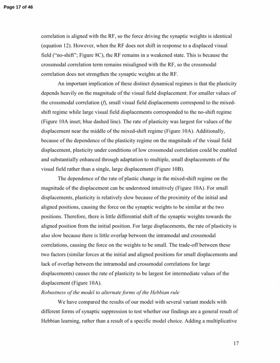
An important implication of these distinct dynamical regimes is that the plasticity
depends heavily on the magnitude of the visual field displacement. For smaller values of
the crossmodal correlation (f), small visual field displacements correspond to the mixed-
shift regime while large visual field displacements corresponded to the no-shift regime
(Figure 10A inset; blue dashed line). The rate of plasticity was largest for values of the
displacement near the middle of the mixed-shift regime (Figure 10A). Additionally,
because of the dependence of the plasticity regime on the magnitude of the visual field
displacement, plasticity under conditions of low crossmodal correlation could be enabled
and substantially enhanced through adaptation to multiple, small displacements of the
visual field rather than a single, large displacement (Figure 10B).
The dependence of the rate of plastic change in the mixed-shift regime on the
magnitude of the displacement can be understood intuitively (Figure 10A). For small
displacements, plasticity is relatively slow because of the proximity of the initial and
aligned positions, causing the force on the synaptic weights to be similar at the two
positions. Therefore, there is little differential shift of the synaptic weights towards the
aligned position from the initial position. For large displacements, the rate of plasticity is
also slow because there is little overlap between the intramodal and crossmodal
correlations, causing the force on the weights to be small. The trade-off between these
two factors (similar forces at the initial and aligned positions for small displacements and
lack of overlap between the intramodal and crossmodal correlations for large
displacements) causes the rate of plasticity to be largest for intermediate values of the
displacement (Figure 10A).
Robustness of the model to alternate forms of the Hebbian rule
We have compared the results of our model with several variant models with
different forms of synaptic suppression to test whether our findings are a general result of
Hebbian learning, rather than a result of a specific model choice. Adding a multiplicative
Page 17 of 46
18
normalization of the synaptic weights to the model does not change the winner-take-all
behavior (“Alternate Form A”, Fig. 11A,B). Likewise, implementing the competition
across synapses by a sliding threshold, similar to the BCM model, rather than by the
subtractive suppressive term, does not alter the finding of winner-take-all dynamics
(“Alternate Form B”, Fig. 11C,D).
In order to test whether our results depend critically on the choice of nonlinearity,
we compared the results of the model with a variant model that used an alternate form of
the nonlinearity. Specifically, we replaced the threshold nonlinearity with a sigmoidal
nonlinearity (“Alternate Form C”, Figure 11E,F). We found that winner-take-all
behavior persists even with this very different form of the nonlinearity.
Plasticity dynamics for parameters chosen to approximate RF properties in barn owl OT
So far, we have explored the dynamics of the model under the conditions that the
auditory presynaptic activity is slightly broader than the visual (b=1.5) and the total
strength of the presynaptic activity are identical (k=1). These parameter values allow for a
clear differentiation between the three dynamic regimes. However, in experiments, much
greater differences between RF properties have been reported. For example, in the optic
tectum of the barn owl, auditory RFs are three times broader than visual RFs (half-max
auditory RF: 30o; half-max visual RF: 10o) (Knudsen 1982). We chose model parameters
for the presynaptic activity to reflect these postsynaptic RF widths. However, the strength
of the responses across modalities have not been reported. Therefore, we chose a value
for auditory RF strength that was 50% larger than that of visual RF strength, a difference
that was chosen to minimize the asymmetry in the resulting plasticity. For the model
parameters that reflect these conditions (b=3.8; k=1.5; φ=23o), although the dynamics are
in the mixed-shift regime, there is still an extreme asymmetry in the plasticity expressed
by each modality: the visual RF only shifts by 2o, while the auditory shifts by 21o (Figure
12). Thus, for these values of the presynaptic activity, the model behaves qualitatively
similarly to the winner-take-all regime, with the auditory modality exhibiting the vast
majority of the plasticity.
Discussion.
Page 18 of 46

19
In this work, we used a Hebbian model to explore the synaptic plasticity that
results from a spatial displacement of one input representation relative to another. Our
main discovery is that equal capacities for Hebbian plasticity in two input channels does
not result in equal plasticity in the two channels under the vast majority of conditions.
Small differences in the relative strength or width of RFs between the two channels has a
dramatic impact on the plasticity that occurs, with the channel with the weaker or broader
RFs exhibiting most or all of the plasticity. These principles, which are robust to the
specific form of the model, apply not only to the maintenance of spatial registry across
inputs, but also to the experience-dependent emergence of aligned representations in
developing circuits.
Our model predicts different regimes of plasticity depending on the size of the
sensory displacements and the strength of the correlation across the input channels. When
the displacement is large and the crossmodal correlation is strong, our model results in
winner-take-all dynamics, with all plasticity being expressed by the weaker or more
broadly tuned channel. In the winner-take-all regime, the dominant process is a decline of
the receptive field at the original position and a concomitant growth of the receptive field
at the new position (for example, Figure 4B). Even in this regime, the dynamics may be
complex, with, for example, initial increases in the synaptic weights at the aligned
positions for both channels (for example, Figure 4B) before plasticity in one of the
channels takes over. When the displacement is small, the mixed-shift regime occurs. In
the mixed-shift regime, the process is dominated by a gradual shift of both receptive
fields from their initial positions to the aligned positions. When the displacements are
large and the correlation is small, the no-shift regime occurs.
Reports in the tectum of juvenile barn owls indicate that both a jump in the RF to
a new position (winner-take-all) and a gradual shift of the RF position (mixed-shift) exist
in response to the same visual field displacement (Brainard and Knudsen 1995). During
the course of plasticity, at some sites, auditory RFs are bimodal, with a peak at both the
original and the new position, suggestive of winner-take-all dynamics (a jump in the
auditory RF rather than a gradual shift). Meanwhile, at other sites, auditory RFs shifted
to intermediate degrees, which is suggestive of mixed-shift dynamics. These differences
may reflect local differences in RF width and strength in a circuit operating near the
Page 19 of 46

20
boundary between mixed-shift and winner-take-all regimes. Future experiments should
vary the magnitude of the displacement and look for a transition between the dynamical
regimes, as well as a relationship between the auditory and visual RF properties at a
particular site and the dynamics expressed at that site.
The observed asymmetry in the amount of plasticity expressed by each input
channel is a purely dynamical phenomenon: when the input from one channel is
displaced, the transient force on the synaptic weights of the weaker or more broadly
tuned channel is stronger than the force on the synaptic weights of the stronger or more
sharply tuned channel, giving rise to a strong imbalance in the trajectories of the synaptic
plasticity across the two channels. In the winner-take-all regime, the force that drives
plasticity is present only at the new location, but vanishes at intermediate locations. The
force vanishes at intermediate locations because of the nonlinearity in the learning rule,
coupled with a lack of overlap between the intramodal and crossmodal terms for large
displacements. Because of this, there is no strengthening of the synaptic weights at
intermediate locations, but instead there is a strengthening of the weights at the new
location for the modality experiencing the stronger force.
The finding of winner-take-all plasticity dynamics holds not only for our main
Hebbian model, but also for the three alternate Hebbian models we presented. In our
main model, the relative mean strength of the synaptic weights, which is determined by
both the relative strength and width of the presynaptic activity, is a good predictor of
which modality shifted (Figure 6, red versus black line). It remains to be explored
whether the relative mean weights or other criteria determine the 'winning' modality in
the three alternate models. In particular, for the case of the multiplicative normalization
(Alternate Model A), the relative mean strength of synaptic weight is immaterial since
the weights are normalized at every iteration such that their mean strengths are identical
for the two modalities.
Comparison to previous theoretical studies
An advantage of our Hebbian learning rule compared to previous rules is that the
synaptic normalization is not a hard constraint. In other words, the mean strength of the
weights is not fixed to a particular value, a demand that is biologically unlikely. Instead,
Page 20 of 46

21
the overall strength of the weight is determined by the nonlinearity and the subtractive
suppressive terms, which result in an approximate normalization. In contrast to many
previous approaches, this yields synaptic weight profiles that are spatially constrained,
smooth and not saturated at their maximum values.
Another novel feature of our model is that the synaptic suppressive terms are is
local to each modality (see eq. 11), rather than the fully global competition across
modalities used in most previous competitive Hebbian models, such as those describing
the development of ocular dominance columns (Miller 1996). Because of this difference,
in our model, both input channels are represented by the postsynaptic cell, whereas in the
previous models, ultimately only one of the two inputs channels drives the postsynaptic
cell. This explains why our model does not reduce to previous models of ocular
dominance plasticity (e.g. (Miller 1996)) when the crossmodal correlation is zero (f=0).
In order for the postsynaptic neuron to be driven by both input modalities, the
exact form of this intramodal competition is not important. What is important is that the
competition within a modality is stronger than the one across modalities. This condition
makes sense for all circuits that must combine information across input channels. An
important question is whether such a specific competition is biologically realized. We
hypothesize that in the case of the optic tectum, synaptic terminals from different input
modalities segregate on different parts of the dendritic tree of the tectal neuron. If true, a
local homeostatic suppressive term may provide the required mechanism. There is both
experimental and theoretical evidence in support of such a mechanism. Synaptic
normalization has recently been shown to occur independently at different synapses (Hou
et al. 2008), although there is evidence of more global mechanisms as well (Ibata et al.
2008). Additionally, a theoretical study found that if synaptic normalization is based on
local activity, then the resulting learning rule normalizes weights separately in different
dendritic compartments (Rabinowitch and Segev 2006).
Our approach differs from previous theoretical studies of crossmodal plasticity in
the barn owl. A previous Hebbian model reproduced experimental plasticity results based
on the assumption that visual connections were not capable of plasticity (Gelfand et al.
1988). Another model involved a spike timing based mechanism to preferentially bias the
circuit towards auditory (and not visual) plasticity (Mysore and Quartz 2005). Based on
Page 21 of 46
22
the results of our model, such assumptions may be unnecessary: differences in receptive
field properties may be sufficient to lead to a great asymmetry in the division of plasticity
across input channels. Another model assumed that auditory synapses were strengthened
by a reward signal that was activated whenever the animal successfully foveated a target
(Rucci et al. 1997), a mechanism that has not been supported by subsequent experiments
(Hyde and Knudsen 2001).
In contrast to mechanistic approaches, other studies have implemented functional
approaches, maximizing the mutual information between the stimulus and the neural
output. They achieved plasticity of the auditory and not the visual RFs based on the
assumption that either the signal-to-noise ratio (Kardar and Zee 2002) or the strength
(Atwal 2004) of the auditory inputs is much less than that of the visual inputs.
Relationship to experimental findings
When inputs have been displaced in experimental systems, the resulting plasticity
is often asymmetrical. For example, when barn owls are fitted with optical displacing
prisms, auditory plasticity reinstates crossmodal alignment, while visual plasticity has not
been observed, even though visual plasticity in the tectum has been reported in other
species following other manipulations. Similarly, when juvenile frogs are raised with a
rotated eye, plasticity of the input from the ipsilateral eye reinstates binocular alignment.
In both cases, there is a dramatic asymmetry in the plasticity exhibited by the two input
channels.
Our findings suggest that the imbalance of plasticity across input channels in
these experiments could be explained mechanistically by differences in RF properties of
the two channels. In the barn owl optic tectum, a site of crossmodal realignment (DeBello
and Knudsen 2004), auditory RFs are three times broader than visual RFs (Knudsen
1982). According to our model, this substantial difference in the RF width would cause
auditory RFs to shift by the entire displacement in the winner-take-all regime and to shift
by most of the displacement in the mixed-shift regime. Another site of auditory plasticity
in the system is the external nucleus of the inferior colliculus (ICX), which is one step
earlier in the auditory processing stream from the optic tectum. Given that the optic
tectum exhibits plasticity in owls that show no plasticity in the ICX (DeBello and
Knudsen 2004), and that the optic tectum is required for plasticity in the ICX (Hyde and
Page 22 of 46

23
Knudsen 2001), it is possible that the plasticity initially occurs in the optic tectum by the
mechanism described here, and then propagates back to the ICX.
The imbalance of plasticity observed in the frog optic tectum, a site of binocular
realignment, could also be explained by differences in RF properties. Most sites are
driven more strongly by inputs from the contralateral rather than the ipsilateral eye
(Gaillard 1985). As we have shown, these differences in RF properties are sufficient to
cause the observed asymmetry in RF plasticity, where the contralateral, and not the
ipsilateral, RFs are plastic.
In experimental models, an important factor that affects the capacity for plasticity
is the magnitude of the spatial displacement imposed on one of the input channels. For
both adult barn owls adapting to auditory-visual misalignments, as well as frogs adapting
to binocular misalignments, plasticity is enhanced through training with multiple, smaller
displacements (Keating et al. 1975; Keating and Grant 1992; Linkenhoker and Knudsen
2002). Our computational model reproduces the enhanced plasticity resulting from
incremental training (Figure 10B). The inability to adapt to large displacements follows
from the fact that as displacements increase, the model circuit transitions from the mixed-
shift to the no-shift regime (Figure 9A).
In our computational model, the strength of the crossmodal correlation plays an
important role in determining the nature of the plasticity. The behavioral state of the
animal during the period of plasticity could affect the strength of the crossmodal
correlation. For example, during hunting, owls exhibit heightened attention to certain
bimodal stimuli, e.g. a scurrying mouse. Attention is known to increase firing rates
substantially (Desimone and Duncan 1995; Knudsen 2007; Reynolds and Chelazzi 2004).
Higher firing rates in response to bimodal stimuli would result in a stronger crossmodal
correlation. As the crossmodal correlation increases, the dynamics transition from the no-
shift to the winner-take-all regime (Figure 9A). This could explain the observation that
adult owls have a greater capacity for plasticity when they are allowed to hunt live mice
(Bergan et al. 2005).
Testable predictions for future experiments
One prediction of our model is that visual plasticity in the barn owl system should
be maximized in the incremental training experiments because, in that case, the system
Page 23 of 46

24
should be in the mixed-shift regime. Gradual shifts in the auditory receptive field
position, as predicted by the mixed-shift regime, have indeed been observed in the optic
tectum of the barn owl (Brainard and Knudsen 1995). However, shifts in visual receptive
fields were not reported. This can be explained by the fact that auditory fields are three
times wider than visual RFs (Knudsen 1982). Therefore, according to the model, there
should be very little change in the visual RF position, on the order of 1o. This magnitude
of shift is well below the resolution of previous measurements. Future experiments could
test for effects of incremental training on visual RFs in the tectum.
A second prediction of our model is that manipulating the relative quality of
auditory and visual stimuli during learning should change the division of plasticity across
the two modalities. For example, if owls were reared with both diffusing and displacing
lenses, such that visual responses were significantly weaker than auditory responses,
plasticity of visual RFs should result.
A third prediction is that responses should weaken in animals that do not adjust to
the displacement of the visual field, as in Figure 8C. Adult barn owls, which are normally
not plastic in response to experience with a displaced visual field, should have weaker
responses after experience with misaligned bimodal inputs in comparison to control
animals. Indeed, weakened auditory responses in optic tecta that do not have adaptively
shifted auditory RFs has been reported anecdotally (Brainard and Knudsen 1998).
Another example of plasticity occurs within the auditory system without reference
to a visual input (Miller and Knudsen 2003). Plasticity occurs in the auditory thalamus
after barn owls are fitted with an acoustic filtering device that alters auditory spatial cues
in a frequency dependent manner. In response to these devices, the tuning of each
frequency channel shifts appropriately to regain spatial alignment across frequency
channels. The division of the adaptive plasticity across frequency channels is unknown.
Our model predicts that, under these conditions, the frequency channels with the broader
or weaker RFs will be the ones to shift their patterns of inputs.
Page 24 of 46

25
Figure Legends.
Figure 1: Schematic diagram of the model. Left: Non-displaced projection of the
visual field. Right: Displaced projection of the visual field. Visual space projects
topographically onto visual presynaptic neurons (“visual presynaptic layer”). Auditory
space is represented topographically by auditory presynaptic neurons (“auditory
presynaptic layer”). Both the visual and auditory presynaptic layers connect via synapses
with a postsynaptic neuron. The model explored the effect of a displacement of the
projection of the visual field onto the visual presynaptic layer on the patterns of auditory
and visual synaptic weights on the postsynaptic neuron.
Figure 2: Examples of activity in the presynaptic layers. Left: When the projection of
the visual field is not displaced, visual and auditory stimuli originating at 0o in space (red
square for visual; blue square for auditory) activate the corresponding regions in the
visual and auditory presynaptic layers with a Gaussian distribution of activity. The height
of the vertical bars in the presynaptic layers denotes the strength of the activity. Right:
When the projection of the visual field was displaced, stimuli originating from the same
location in space activated misaligned regions in the visual and auditory presynaptic
layers.
Figure 3: Examples of intramodal and crossmodal correlations. A. The auditory ( aaijC ,
blue trace) and visual ( vvijC , red trace) intramodal correlations. B. The crossmodal
correlations ( avijC ) when the visual field is not displaced (φ = 0o, solid trace) and when
the visual field is displaced (φ = 45o, dotted trace). Other parameters: k = 1, b = 1.5, f =
0.5.
Figure 4: Receptive field plasticity when auditory and visual presynaptic activity
profiles are identical (k = 1, b = 1). A. Identical auditory (blue) and visual (red) RFs for
the postsynaptic neuron, after training the model with a non-displaced visual field. B.
Visual (top) and auditory (bottom) RFs for the postsynaptic neuron as a function of time.
Page 25 of 46

26
Before time 0, the visual field was not displaced. At time 0 (dashed line), the projection
of the visual field was displaced by 45o. In this run of the model, the visual RF, and not
the auditory RF, shifted to compensate for the visual field displacement. C. Same as in B,
but in this run of the model, the auditory RF, and not the visual RF, shifted to compensate
for the visual field displacement. Other parameters: f = .5; φ = 45o.
Figure 5: Winner-take-all plasticity for non-identical auditory and visual presynaptic
activity profiles. A,B. Total auditory presynaptic activity, summed across all neurons,
was weaker than visual activity, but the widths of the activity profiles were identical (k =
.9, b = 1). C,D. The auditory presynaptic activity profile was broader than visual, but the
total strength, summed across the presynaptic layers, was identical (k = 1, b = 1.5). A,C.
Auditory and visual RFs for the postsynaptic neuron, following training the model with a
non-displaced visual field. B,D. Visual (top) and auditory (bottom) RFs for the
postsynaptic neuron as a function of time. Before time 0, the visual field was non-
displaced. At time of 0 (dashed line), the visual field was displaced by 45o. In both cases,
only the auditory RF shifted in response to the displaced visual field. Other parameters: f
= .5; φ = 45o.
Figure 6: The modality that shifted depended on the relative width (b) and strength (k)
of the presynaptic activity profiles. The boundary between the region of visual versus
auditory plasticity is denoted by the black solid line. To the right of the solid line, only
the visual RFs shifted; to the left, only the auditory RF shifted. The boundary between the
regions in which the visual versus auditory synaptic weights were weaker is denoted by
the red dotted line. To the right of the dotted line, the visual synaptic weights (averaged
across all synapses) were weaker; to the left, the auditory synaptic weights (averaged
across all synapses) were weaker. Other parameters: f = .5, φ = 45o.
Figure 7: Distribution of synaptic weights and correlations convolved with the weights
at various timepoints. The left column: before the visual field displacement; the central
column: immediately after the visual field displacement (φ = 45o); the right column: after
adaptation to the displacement. A-C. The distribution of synaptic weights, with red lines
Page 26 of 46

27
corresponding to visual weights and blue lines corresponding to auditory weights. D-F.
The intramodal correlations convolved with the appropriate weights, from equation 12.
G-I. The crossmodal correlation convolved with the appropriate weights, from equation
12. In D-I, the red lines represent the term that contributes to visual plasticity (bottom
line in equation 12), and the blue line represent the term that contributes to auditory
plasticity (top line in equation 12). Other parameters: f = .5; k = 1, b = 1.5.
Figure 8: Two additional regimes of plasticity dynamics in response to a displacement
of the visual field. A. In the mixed-shift regime, the RFs for both input channels shifted
continuously, and both RFs shifted to some extent. The mixed shift regime occurred
when the displacement was small (this example: φ = 15o), and the crossmodal correlation
was low (this example: f = .1). Before time 0, the visual field was not displaced. At time
of 0 (dashed line), the visual field was displaced by 15o. Other parameters: k = 1, b = 1.5.
B. Relative plasticity across input channels in the mixed shift regime as a function of the
relative width (b) and strength (k) of the presynaptic activity profiles, quantified as
follows: (Shiftauditory – Shiftvisual)/(Shiftauditory + Shiftvisual). White asterisk represents value
of b and k used in the other panels. C. In the no-shift regime, neither the auditory nor the
visual RF shifted in response to the displaced visual field. The no-shift regime occurred
when the visual field displacement was large (this example: φ = 45o) and the crossmodal
correlation was low (this example: f = .1). Other parameters: k = 1, b = 1.5.
Figure 9: Plasticity regimes depended on the magnitude of the visual field
displacement and on the strength of the crossmodal correlation. A. Phase diagram
showing the boundaries between the no-shift, mixed-shift, and winner-take-all regimes as
a function of the visual field displacement (φ) and the correlation strength (f). B. Force on
the auditory (top panel) and visual (bottom panel) synaptic weights for the winner-take-
all regime (φ = 45o, f = .5). C. Force on the visual (top panel) and auditory (bottom
panel) synaptic weights for the no-shift regime (φ = 45o, f = .1). D. Force on the auditory
(top panel) and visual (bottom panel) synaptic weights for the mixed-shift regime (φ =
15o, f = .1). In B-D, arrows indicate the initial position of the RF immediately after the
Page 27 of 46

28
visual field displacement (initial), and the position of the RF if it were to shift fully
(aligned). Other parameters: k = 1; b = 1.5.
Figure 10: Kinetics of plasticity. A. Average rate of RF plasticity as a function of the
magnitude of the visual field displacement (f = .1). Inset: dotted blue line shows the
transect through the phase diagram in Fig. 8A that corresponds to the parameters used to
generate this data. B. Total shift (summed across both modalities) in response either to a
large displacement of the visual field applied at time 0, in which case no shift occurred
(solid black line; φ = 45o, f = .1) or to three sequential displacements of one third the size,
applied at times 0, 15, and 30 (solid red line; φ = 15o, f = .1). Dotted lines indicate the
magnitude of the visual field displacement. Other parameters: k = 1; b = 1.5.
Figure 11: Alternate forms of the model reproduce winner-take-all dynamics. A,B. A
multiplicative normalization was introduced to the original model (see Methods,
“Alternate Form A”; Jvv=10, c=.5; f=1). C,D. A variant of a BCM normalization was
introduced to the original model (see Methods, “Alternate Form B”; Jvv=1.2, JBCM=.1; f
=1). E,F. A sigmoidal nonlinearity replaced the threshold nonlinearity (see Methods,
“Alternate Form C”; Jvv=100; I=1000; β=.1; f=.5). A,C,E. Auditory and visual RFs for
the postsynaptic neuron, following training the model with a non-displaced visual field.
B,D, F. Visual (top) and auditory (bottom) RFs for the postsynaptic neuron as a function
of time. Before time 0, the visual field was non-displaced. At time of 0 (dashed line), the
visual field was displaced by 45o. In all cases, only the auditory RF shifted in response to
the displaced visual field. Other parameters: k = 1; b = 1.5; φ = 45o.
Figure 12: Dynamics for parameter values that approximate the RF properties in the
barn owl optic tectum. Auditory and visual presynaptic activity were chosen to reflect the
values in the optic tectum. A. Auditory and visual RFs for the postsynaptic neuron,
following training the model with a non-displaced visual field. The width at half-max is
30o for the auditory RF and 10o for the visual RF. B. Visual (top) and auditory (bottom)
RFs for the postsynaptic neuron as a function of time. Before time 0, the visual field was
non-displaced. At time of 0 (dashed line), the visual field was displaced by 45o. In both
Page 28 of 46

29
cases, only the auditory RF shifted in response to the displaced visual field. Other
parameters: b=3.8; k=1.5; f= .5; φ = 23o; σav=3o.
Acknowledgements: We would like the thank the Methods in Computational Neuroscience course at the Marine Biological Laboratories for the hospitality and support. Additionally, thanks to M. Goldman, J. Bergan, D. Winkowski, S. Mysore, and A. Asadollahi for helpful comments on this manuscript. IBW and EIK were supported by NIH grants; IBW received additional support from an NSF Graduate Research Fellowship. HS was partially supported by a grant from the Israeli Science Foundation.
REFERENCES
Atwal GS. Dynamic plasticity in coupled avian midbrain maps. Phys Rev E Stat Nonlin Soft Matter Phys 70: 061904, 2004.Bergan JF, Ro P, Ro D, and Knudsen EI. Hunting increases adaptive auditory map plasticity in adult barn owls. J Neurosci 25: 9816-9820, 2005. Bienenstock EL, Cooper LN, and Munro PW. Theory for the development of neuron selectivity: orientation specificity and binocular interaction in visual cortex. J Neurosci 2:32-48, 1982. Brainard MS and Knudsen EI. Dynamics of visually guided auditory plasticity in the optic tectum of the barn owl. J Neurophysiol 73: 595-614, 1995. Brainard MS and Knudsen EI. Sensitive periods for visual calibration of the auditory space map in the barn owl optic tectum. J Neurosci 18: 3929-3942, 1998. Constantine-Paton M and Law MI. Eye-specific termination bands in tecta of three-eyed frogs. Science 202: 639-641, 1978. DeBello WM and Knudsen EI. Multiple sites of adaptive plasticity in the owl's auditory localization pathway. J Neurosci 24: 6853-6861, 2004. Desimone R and Duncan J. Neural mechanisms of selective visual attention. Annu Rev Neurosci 18: 193-222, 1995. Engert F, Tao HW, Zhang LI, and Poo MM. Moving visual stimuli rapidly induce direction sensitivity of developing tectal neurons. Nature 419: 470-475, 2002. Gaillard F. Binocularly driven neurons in the rostral part of the frog optic tectum. JComp Physiol [A] 157: 47-55, 1985. Gelfand JJ, Pearson JC, Spence CD, and Sullivan WE. Multisensor integration in biological systems. IEEE International Symposium on Intelligent Control, Arlington, VA, USA, 1988, p. 147-153. Gold JI and Knudsen EI. Hearing impairment induces frequency-specific adjustments in auditory spatial tuning in the optic tectum of young owls. J Neurophysiol 82: 2197-2209, 1999. Hou Q, Zhang D, Jarzylo L, Huganir RL, and Man HY. Homeostatic regulation of AMPA receptor expression at single hippocampal synapses. Proc Natl Acad Sci U S A 105: 775-780, 2008. Hyde PS and Knudsen EI. A topographic instructive signal guides the adjustment of the auditory space map in the optic tectum. J Neurosci 21: 8586-8593, 2001.
Page 29 of 46

30
Ibata K, Sun Q, and Turrigiano GG. Rapid synaptic scaling induced by changes in postsynaptic firing. Neuron 57: 819-826, 2008. Kardar M and Zee A. Information optimization in coupled audio-visual cortical maps. Proc Natl Acad Sci U S A 99: 15894-15897, 2002. Keating MJ, Beazley L, Feldman JD, and Gaze RM. Binocular interaction and intertectal neuronal connexions: dependence upon developmental stage. Proc R Soc Lond B Biol Sci 191: 445-466, 1975. Keating MJ and Grant S. The Critical Period for Experience-dependent Plasticity in a System of Binocular Visual Connections in Xenopus laevis: Its Temporal Profile and Relation to Normal Developmental Requirements. Eur J Neurosci 4: 27-36, 1992. Knudsen EI. Auditory and visual maps of space in the optic tectum of the owl. JNeurosci 2: 1177-1194, 1982. Knudsen EI. Fundamental Components of Attention. Annu Rev Neurosci, 2007. Knudsen EI. Instructed learning in the auditory localization pathway of the barn owl. Nature 417: 322-328, 2002. Linkenhoker BA and Knudsen EI. Incremental training increases the plasticity of the auditory space map in adult barn owls. Nature 419: 293-296, 2002. Miller GL and Knudsen EI. Adaptive plasticity in the auditory thalamus of juvenile barn owls. J Neurosci 23: 1059-1065, 2003. Miller KD. Synaptic economics: competition and cooperation in synaptic plasticity. Neuron 17: 371-374, 1996. Miller KD, MacKay, D.J.C. The role of constraints in Hebbian learning. Neural Computation 6: 100-126, 1994. Mysore SP and Quartz SR. Modeling structural plasticity in the barn owl auditory localization system with a spike-time dependent Hebbian learning rule. IEEE International Joint Conference on Neural Networks, 2005., 2005, p. 2766- 2771.Rabinowitch I and Segev I. The interplay between homeostatic synaptic plasticity and functional dendritic compartments. J Neurophysiol 96: 276-283, 2006. Reh TA and Constantine-Paton M. Eye-specific segregation requires neural activity in three-eyed Rana pipiens. J Neurosci 5: 1132-1143, 1985. Reynolds JH and Chelazzi L. Attentional modulation of visual processing. Annu Rev Neurosci 27: 611-647, 2004. Rucci M, Tononi G, and Edelman GM. Registration of neural maps through value-dependent learning: Modeling the alignment of auditory and visual maps in the barn owl's optic tectum. Journal of Neuroscience 17: 334-352, 1997. Udin SB and Fawcett JW. Formation of topographic maps. Annu Rev Neurosci 11: 289-327, 1988. Udin SB and Grant S. Plasticity in the tectum of Xenopus laevis: binocular maps. Prog Neurobiol 59: 81-106, 1999. Zhang LI, Tao HW, Holt CE, Harris WA, and Poo M. A critical window for cooperation and competition among developing retinotectal synapses. Nature 395: 37-44, 1998.
Page 30 of 46

Figure 1: Schematic diagram of the model. Left: Non-displaced projection of the visual field. Right: Displaced projection of the visual field. Visual space projects topographically
onto visual presynaptic neurons ("visual presynaptic layer"). Auditory space is represented topographically by auditory presynaptic neurons ("auditory presynaptic layer"). Both the visual and auditory presynaptic layers connect via synapses with a
postsynaptic neuron. The model explored the effect of a displacement of the projection of the visual field onto the visual presynaptic layer on the patterns of auditory and visual
synaptic weights on the postsynaptic neuron. 215x279mm (600 x 600 DPI)
Page 31 of 46

Figure 2: Examples of activity in the presynaptic layers. Left: When the projection of the visual field is not displaced, visual and auditory stimuli originating at 0 in space (red square for visual; blue square for auditory) activate the corresponding regions in the
visual and auditory presynaptic layers with a Gaussian distribution of activity. The height of the vertical bars in the presynaptic layers denotes the strength of the activity. Right: When the projection of the visual field was displaced, stimuli originating from the same
location in space activated misaligned regions in the visual and auditory presynaptic layers.
215x279mm (600 x 600 DPI)
Page 32 of 46

Figure 3: Examples of intramodal and crossmodal correlations. A. The auditory ( Caaij, blue
trace) and visual (Cvvij , red trace) intramodal correlations. B. The crossmodal correlations
(Cavij) when the visual field is not displaced ( = 0 , solid trace) and when the visual
field is displaced ( = 45 , dotted trace). Other parameters: k = 1, b = 1.5, f = 0.5. 215x279mm (600 x 600 DPI)
Page 33 of 46
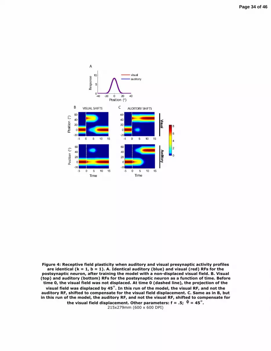
Figure 4: Receptive field plasticity when auditory and visual presynaptic activity profiles are identical (k = 1, b = 1). A. Identical auditory (blue) and visual (red) RFs for the
postsynaptic neuron, after training the model with a non-displaced visual field. B. Visual (top) and auditory (bottom) RFs for the postsynaptic neuron as a function of time. Before
time 0, the visual field was not displaced. At time 0 (dashed line), the projection of the visual field was displaced by 45 . In this run of the model, the visual RF, and not the
auditory RF, shifted to compensate for the visual field displacement. C. Same as in B, but in this run of the model, the auditory RF, and not the visual RF, shifted to compensate for
the visual field displacement. Other parameters: f = .5; = 45 .215x279mm (600 x 600 DPI)
Page 34 of 46

Figure 5: Winner-take-all plasticity for non-identical auditory and visual presynaptic activity profiles. A,B. Total auditory presynaptic activity, summed across all neurons, was weaker than visual activity, but the widths of the activity profiles were identical (k = .9, b = 1). C,D. The auditory presynaptic activity profile was broader than visual, but the total
strength, summed across the presynaptic layers, was identical (k = 1, b = 1.5). A,C. Auditory and visual RFs for the postsynaptic neuron, following training the model with a
non-displaced visual field. B,D. Visual (top) and auditory (bottom) RFs for the postsynaptic neuron as a function of time. Before time 0, the visual field was non-
displaced. At time of 0 (dashed line), the visual field was displaced by 45 . In both cases, only the auditory RF shifted in response to the displaced visual field. Other parameters: f
= .5; = 45 .215x279mm (600 x 600 DPI)
Page 35 of 46

Page 36 of 46

Figure 6: The modality that shifted depended on the relative width (b) and strength (k) of the presynaptic activity profiles. The boundary between the region of visual versus
auditory plasticity is denoted by the black solid line. To the right of the solid line, only the visual RFs shifted; to the left, only the auditory RF shifted. The boundary between the
regions in which the visual versus auditory synaptic weights were weaker is denoted by the red dotted line. To the right of the dotted line, the visual synaptic weights (averaged across all synapses) were weaker; to the left, the auditory synaptic weights (averaged
across all synapses) were weaker. Other parameters: f = .5, = 45 .215x279mm (600 x 600 DPI)
Page 37 of 46

Figure 7: Distribution of synaptic weights and correlations convolved with the weights at various timepoints. The left column: before the visual field displacement; the central column: immediately after the visual field displacement ( = 45 ); the right column:
after adaptation to the displacement. A-C. The distribution of synaptic weights, with red lines corresponding to visual weights and blue lines corresponding to auditory weights. D-F. The intramodal correlations convolved with the appropriate weights, from equation
12. G-I. The crossmodal correlation convolved with the appropriate weights, from equation 12. In D-I, the red lines represent the term that contributes to visual plasticity
(bottom line in equation 12), and the blue line represent the term that contributes to auditory plasticity (top line in equation 12). Other parameters: f = .5; k = 1, b = 1.5.
215x279mm (600 x 600 DPI)
Page 38 of 46

Page 39 of 46

Figure 8: Two additional regimes of plasticity dynamics in response to a displacement of the visual field. A. In the mixed-shift regime, the RFs for both input channels shifted
continuously, and both RFs shifted to some extent. The mixed shift regime occurred when the displacement was small (this example: = 15o), and the crossmodal correlation was low (this example: f = .1). Before time 0, the visual field was not displaced. At time of 0 (dashed line), the visual field was displaced by 15o. Other parameters: k = 1, b = 1.5. B. Relative plasticity across input channels in the mixed shift regime as a function of the relative width (b) and strength (k) of the presynaptic activity profiles, quantified as
follows: (Shift_auditory - Shift_visual)/(Shift_auditory + Shift_visual). White asterisk represents value of b and k used in the other panels. C. In the no-shift regime, neither the
auditory nor the visual RF shifted in response to the displaced visual field. The no-shift regime occurred when the visual field displacement was large (this example: = 45o)
and the crossmodal correlation was low (this example: f = .1). Other parameters: k = 1, b
Page 40 of 46

= 1.5. 215x279mm (600 x 600 DPI)
Page 41 of 46

Figure 9: Plasticity regimes depended on the magnitude of the visual field displacement and on the strength of the crossmodal correlation. A. Phase diagram showing the
boundaries between the no-shift, mixed-shift, and winner-take-all regimes as a function of the visual field displacement ( ) and the correlation strength (f). B. Force on the
auditory (top panel) and visual (bottom panel) synaptic weights for the winner-take-all regime ( = 45 , f = .5). C. Force on the visual (top panel) and auditory (bottom panel) synaptic weights for the no-shift regime ( = 45 , f = .1). D. Force on the auditory (top
panel) and visual (bottom panel) synaptic weights for the mixed-shift regime ( = 15 , f= .1). In B-D, arrows indicate the initial position of the RF immediately after the visual field displacement (initial), and the position of the RF if it were to shift fully (aligned).
Other parameters: k = 1; b = 1.5. 215x279mm (600 x 600 DPI)
Page 42 of 46

Page 43 of 46

Figure 10: Kinetics of plasticity. A. Average rate of RF plasticity as a function of the magnitude of the visual field displacement (f = .1). Inset: dotted blue line shows the
transect through the phase diagram in Fig. 8A that corresponds to the parameters used to generate this data. B. Total shift (summed across both modalities) in response either to a
large displacement of the visual field applied at time 0, in which case no shift occurred (solid black line; = 45 , f = .1) or to three sequential displacements of one third the
size, applied at times 0, 15, and 30 (solid red line; = 15 , f = .1). Dotted lines indicate the magnitude of the visual field displacement. Other parameters: k = 1; b = 1.5.
215x279mm (600 x 600 DPI)
Page 44 of 46

Figure 11: Alternate forms of the model reproduce winner-take-all dynamics. A,B. A multiplicative normalization was introduced to the original model (see Methods, 'Alternate Form A'; Jvv=10, c=.5; f=1). C,D. A variant of a BCM normalization was
introduced to the original model (see Methods, 'Alternate Form B'; Jvv=1.2, JBCM=.1; f =1). E,F. A sigmoidal nonlinearity replaced the threshold nonlinearity (see Methods, 'Alternate
Form C'; Jvv=100; I=1000; =.1; f=.5). A,C,E. Auditory and visual RFs for the postsynaptic neuron, following training the model with a non-displaced visual field. B,D, F. Visual (top) and auditory (bottom) RFs for the postsynaptic neuron as a function of time. Before time 0, the visual field was non-displaced. At time of 0 (dashed line), the
visual field was displaced by 45o. In all cases, only the auditory RF shifted in response to the displaced visual field. Other parameters: k = 1; b = 1.5; = 45o.
215x279mm (600 x 600 DPI)
Page 45 of 46

Figure 12: Dynamics for parameter values that approximate the RF properties in the barn owl optic tectum. Auditory and visual presynaptic activity were chosen to reflect the values in the optic tectum. A. Auditory and visual RFs for the postsynaptic neuron,
following training the model with a non-displaced visual field. The width at half-max is 30o for the auditory RF and 10o for the visual RF. B. Visual (top) and auditory (bottom)
RFs for the postsynaptic neuron as a function of time. Before time 0, the visual field was non-displaced. At time of 0 (dashed line), the visual field was displaced by 23o. Other
parameters: b=3.8; k=1.5; f= .5; = 23o; Jav=3. 215x279mm (600 x 600 DPI)
Page 46 of 46


