Embed Size (px)
Citation preview

NeuroImage 114 (2015) 57–70
Contents lists available at ScienceDirect
NeuroImage
j ourna l homepage: www.e lsev ie r .com/ locate /yn img
A jackknife approach to quantifying single-trial correlation betweencovariance-based metrics undefined on a single-trial basis
Craig G. Richter a,b,⁎, William H. Thompson a,c, Conrado A. Bosman d,e, Pascal Fries a,e
a Ernst Strüngmann Institute (ESI) for Neuroscience in Cooperation with Max Planck Society, 60528 Frankfurt, Germanyb Laboratoire de Neurosciences Cognitives, École Normale Supérieure, 75005 Paris, Francec Department of Clinical Neuroscience, Karolinska Institute, 171 76 Stockholm, Swedend Cognitive and Systems Neuroscience Group, Swammerdam Institute for Life Sciences, Center for Neuroscience, University of Amsterdam, 1098 XH Amsterdam, Netherlandse Donders Institute for Brain, Cognition and Behaviour, Radboud University Nijmegen, 6525 EN Nijmegen, Netherlands
⁎ Corresponding author at: Ernst Strüngmann InstitCooperation with Max Planck Society, 60528 Frankfurt, G
E-mail address: [email protected] (C.G. Richter
http://dx.doi.org/10.1016/j.neuroimage.2015.04.0401053-8119/© 2015 The Authors. Published by Elsevier Inc
a b s t r a c t
a r t i c l e i n f oArticle history:Received 27 June 2014Accepted 20 April 2015Available online 24 April 2015
Keywords:Single-trial correlationJackknifeFunctional connectivityCoherenceGranger causalitySpectral analysis
The quantification of covariance between neuronal activities (functional connectivity) requires the observationof correlated changes and therefore multiple observations. The strength of such neuronal correlations may itselfundergo moment-by-moment fluctuations, which might e.g. lead to fluctuations in single-trial metrics such asreaction time (RT), or may co-fluctuate with the correlation betwe'en activity in other brain areas. Yet, quantify-ing the relation between moment-by-moment co-fluctuations in neuronal correlations is precluded by the factthat neuronal correlations are not defined per single observation. The proposed solution quantifies this relationby first calculating neuronal correlations for all leave-one-out subsamples (i.e. the jackknife replications of allobservations) and then correlating these values. Because the correlation is calculated between jackknife replica-tions, we address this approach as jackknife correlation (JC). First, we demonstrate the equivalence of JC toconventional correlation for simulated paired data that are defined per observation and therefore allow thecalculation of conventional correlation. While the JC recovers the conventional correlation precisely, alternativeapproaches, like sorting-and-binning, result in detrimental effects of the analysis parameters. We then explorethe case of relating two spectral correlation metrics, like coherence, that require multiple observation epochs,where the only viable alternative analysis approaches are based on some formof epoch subdivision,which resultsin reduced spectral resolution and poor spectral estimators. We show that JC outperforms these approaches,particularly for short epoch lengths, without sacrificing any spectral resolution. Finally, we note that the JC canbe applied to relate fluctuations in any smooth metric that is not defined on single observations.
© 2015 The Authors. Published by Elsevier Inc. This is an open access article under the CC BY license(http://creativecommons.org/licenses/by/4.0/).
Introduction
Brain activity exhibits a very high degree of moment-to-momentvariability. Activity fluctuations in one brain area are often correlatedto fluctuations in other areas. These inter-areal correlations themselvesmost likely also undergo moment-to-moment fluctuations in strength,and it is an intriguing question whether those fluctuations are relatedto fluctuations in behavior, in the activity of other brain areas, or inthe strength of correlation between other brain areas. Consider the fol-lowing example: Areas A and B might show beta-band coherence, andat the same time areas B and C might show gamma-band coherence.This might lead us to wonder if the interaction between areas A and Bis related to the interaction between B and C. Determining such a rela-tion is highly desirable for neuroimaging applications where the
ute (ESI) for Neuroscience inermany.).
. This is an open access article under
correlation between elements of large-scale networks is an issue ofgreat interest (Park and Friston, 2013; Turk-Browne, 2013). Yet, this isdifficult to achieve, because determining the strength of correlation al-ready entails the observation of changes in one signal and related changesin another signal. Thus, determining correlation requires multiple obser-vations and therefore, the strength of correlation cannot be determinedon a single observation, i.e. it cannot be determined on a moment-by-moment basis. So, is it impossible to relate fluctuations in the correlationstrength between two areas to fluctuations in other parameters?
Here, we present an approach that achieves this: The Jackknife Cor-relation (JC). JC builds on the work of Stahl and Gibbons (2004), whichextended the jackknife method of Miller et al. (1998) to the case ofquantifying correlations between brain potentials and behavioral vari-ables. They demonstrate that correlating jackknife estimates of thelateralized readiness potential to personality metrics is superior tosingle-subject based approaches. JC transfers this rationale to the caseof correlations involving covariance-based metrics, which are strictlynot defined for single observations. JC enables the correlation of these
the CC BY license (http://creativecommons.org/licenses/by/4.0/).

58 C.G. Richter et al. / NeuroImage 114 (2015) 57–70
metrics to other metrics, like RT (that are defined on single observa-tions), but crucially, JC also allows the correlation of these metrics toeach other like in the above example of correlating the A–B beta-bandcoherence to the B–C gamma-band coherence. Thereby, it is an impor-tant new tool for the investigation of functional connectivity.
The jackknife technique successively leaves out each observationonce. Each time one observation is left out, this results in an all-but-one ensemble of observations, called a jackknife replication. Thereby,for N observations, there are N jackknife replications. Each jackknifereplication contains N-1 observations, and thereby allows quantifyingthe correlation strength across those N-1 observations. These correla-tion strengths fluctuate across the N jackknife replications. Becauseeach jackknife replication leaves out only one observation, the varianceacross jackknife replications is small. Yet because each jackknife replica-tion leaves out precisely one observation, the variance across jackknifereplications is a precise transform of the variance across the original ob-servations. Because correlation is driven solely by covariance and nor-malized for the variances of the correlated signals, the correlationbetween jackknife replications is in fact identical to the correlation be-tween the original observations. We will demonstrate this first for sim-ulated data that are defined for each single observation. We proposethat this is an answer to the abovementioned question, namely thatthe same approach can be taken for testingwhether fluctuations in cor-relation are related to other parameters, even though it may not be pos-sible to determine the value of either variable on amoment-by-momentbasis, as is the case for ensemblemetrics such as coherence.We supportthe proposal by simulating data with an autoregressivemodel such thatthe correlation was dependent on a fluctuating pre-determined controlparameter. This pre-specified relation between the control parameterand the correlation was then successfully recovered through JC.
Alternative approaches to computing correlation upon covariance-based metrics
Approaches to this problem can be divided into two classes. The firstseeks to determine a value for the covariance-based metric or each sin-gle trial. The second approach estimates the ensemble metric over sub-groups of trials formed by decomposing the total number of trials intosubensembles. Consider the following example: Supposewewish to in-vestigate the trial-by-trial correlation between reaction time (RT) andinter-areal gamma-band coherence. While RT is defined on each trial,coherence is not. Coherence quantifies the consistency of phase rela-tions across multiple trials, which renders it undefined at the level of asingle trial. The first approach would attempt to determine the coher-ence of each single trial by subdividing each trial into multiple epochsand computing the coherence over each of these sub-segments(Welch, 1967; Lachaux et al., 2000). Alternatively, one could achievethe same single-trial estimate by applying multiple data tapers overthe single epoch (Mitra and Pesaran, 1999). Yet, both methods are lim-ited by the nature of brain dynamics in general, where periods of inter-est are often present for only brief instances, such that single trials aretypically too short to derive multiple spectral estimators, or applylarge numbers of tapers. Another approach to estimating coherence ona single-trial basis, which is in fact closely related to JC, is the use ofjackknife pseudovalues (Womelsdorf et al., 2006). The jackknifepseudovalue is an estimate of the single-trial value of a statistic that isbased on the difference between 1) the statistic calculated across all tri-als (weighted by n) and 2) the statistic calculated on all-but-one trial(weighted by n-1). A problem with the pseudovalue approach canarise e.g. from the following combination of facts: 1) the difference be-tween the all-trial and the leave-one-out estimate is very small, and2)many interestingmetrics, like coherence, carry a sample-size depen-dent bias (Maris et al., 2007), i.e. the coherence biaswill be slightly larg-er for the leave-one-out estimate than for the complete estimate. Whilethe bias from point 2) is small, also the difference from point 1) is small,and this combination can lead to problems with the single-trial
estimate, that necessitate complicated solutions. These problems arefully avoided by JC, because it calculates the correlation directly be-tween the jackknife replications of the statistic without attempting toestimate the statistic on a single trial. If one nevertheless wants to esti-mate coherence on the single trial level, e.g. for illustration purposes,then the pseudovalue approach might be used together with a bias-freemetric of interaction strength, like the recently introduced pairwisephase consistency metric, PPC (Vinck et al., 2010). To summarize,single-trial estimation approaches all suffer from either reduced accura-cy of the estimate, or excessive computational complexity, thus it ismost desirable toworkwith coherence estimates computed overmulti-ple trials.
The second approach does just this andwe address it as sorting-and-binning. Sorting-and-binning can only be used if one of the variables isdefined on the basis of single observations. The observations are sortedand binned according to this (single-observation-defined) variable. Forthis variable, the mean per bin is computed. For the other variable,which is not defined on a single observation, the covariance-basedmet-ric is calculated separately per bin, across the multiple observationswithin each bin. Finally, the correlation between the two metrics iscomputed across the bins. This approach can be found in a largenumber of studies ranging beyond neuroscience. See Liang et al.(2002),Hanslmayr et al. (2007),Womelsdorf et al. (2007) andvanElswijk et al. (2010) as examples of the technique. It's important tonote that if neither quantity over which we wish to perform the corre-lation is defined on a single-observation basis, then this method cannotbe applied, since sorting cannot be performed. JC is not limited in thisway since neither variable need be defined for a single trial. We willfurther investigate the process of sorting-and-binning to illustratesome often overlooked statistical pitfalls of this technique while in par-allel developing the mechanics of JC.
The sorting-and-binning approach
The sorting-and-binning approach proceeds in the following man-ner: Suppose we have 1000 trials. We can sort these according to RT,bin them into 20 bins of 50 trials, calculate the mean RT per bin, calcu-late coherence per bin across the 50 trials in the bin, andfinally calculatethe correlation between RT and coherence across the 20 bins. With thisapproach, the coherence per bin can be computed, because each bincomprises 50 trials. We will demonstrate below that such a binningstrategy carries substantial statistical costs. Suppose we have only 200trials. We do not want to bin them into 20 non-overlapping bins of 10trials each, because 10 trials will result in poor coherence estimates.On the other hand, non-overlapping 50-trial bins will result in only 4bins, which is a very low n for useful correlation. Thus, wemight consid-er overlapping our bins. If the 50-trial bins are overlapped by 40 trials,this furnishes us with 16 bins. We will demonstrate that the combina-tion of binning with overlap incurs further costs.
To simplify this demonstration, we begin with two correlated ran-dom variables, of 1000 trials, that are both defined on a single-trialbasis, such as e.g. the gamma-band power of two brain areas. We usethemean as the statistical operation we apply to each bin. The variableswere generatedwith a covariance of 0.1, which leads to a Pearson corre-lation coefficient of r(998) = 0.1, p b 0.0018. The r-value and p-valuesurfaces (Fig. 1) were computed using a grid of combinations betweenoverlap percentages and bin sizes, which was selected so as to includeonly those combinations that used all of the data with no remainder,i.e. the final bin terminated on the final data sample. This grid is irregu-larly spaced. For a maximum bin size of 250 trials, this resulted in 1286bin/overlap combinations, which each resulted in a Pearson productmoment-correlation coefficient r and significance level p. To establishstatistical stability, these values were evaluated 10,000 times and aver-aged. Correlation coefficients were converted to t-values and assessedfor significance using Student's t-distribution (Rahman, 1968). Theresulting irregular grid of r- and p-values was interpolated to an even

50100
150200
0
50
100
0
0.2
0.4
0.6
0.8
1
r
50 100 150 2000
0.2
0.4
0.6
0.8
1
trials per bin
r
0 20 40 60 800
0.2
0.4
0.6
0.8
1
% overlap
r
50100
150200
0
50
100
0
0.02
0.04
0.06
0.08
0.1
% overlaptrials per bin
p−va
lue
50 100 150 2000
0.02
0.04
0.06
0.08
0.1
trials per bin
p−va
lue
0 20 40 60 800
0.02
0.04
0.06
0.08
0.1
% overlap
p−va
lue
50100
150200
0
50
100
10−10
10−8
10−6
10−4
10−2
100
p−va
lue
50 100 150 200
10−10
10−5
100
trials per bin
p−va
lue
0 20 40 60 80
10−10
10−5
100
% overlap
p−va
lue
A B C
D E F
G H I
% overlaptrials per bin
% overlaptrials per bin
Fig. 1. Parametric examination of the effect of sorting-and-binning on Pearson's product moment correlation coefficient (r), and its statistical significance. A. Parametric surface depicting theeffect on r as the bin size and degree of overlap are varied. B. Correspondingmap of the parametric change in statistical significance (p-value) for the r-values shown in A. C. Same as B, butwithlogarithmic p-value axis. D. The effect of bin size on r shown for three overlap parameters. G. The effect of overlap on r shown for bin sizes of 20 (yellow), 120 (orange) and 245 (red). E, H.Corresponding p-values for D andG. These p-values are false and are depicted only for illustration purposes (seemain text). F, I. Same as E and H, butwith logarithmic p-value axis. The dashedblack line marks the 0.05 significance threshold in all p-value plots. The dashed orange line in H and I shows the correct (Monte-Carlo based) p-values for the middle bin size.
59C.G. Richter et al. / NeuroImage 114 (2015) 57–70
grid with a spacing of 5 trials using Delaunay triangulation. All simula-tions were performed using MATLAB (The MathWorks, Inc.).
We can now examine the various binning/overlap parameteriza-tions (Fig. 1). For the case of zero overlap, Fig. 1 demonstrates that an in-creasing number of trials per bin results in a correlation coefficient thatincreases from the true trial-by-trial value of 0.1 to a value close to 1(blue curve in Fig. 1A). This can be explained by examining the scatterplots in Fig. 2(E, F, I, and J), which show that the residuals (the distanceof each point from the line of best fit) decrease as the bin size increases.This effect is due to the averaging out of random variation in the data.While the large r is not incorrect if considered in the context of its calcu-lation, and it might appeal to a scientist looking for a clear effect, thereare several points that have to be considered: 1) When the r-value iscomputed between the single-trial variables, then the squared r-valuegives the variance in one variable explained by the variance in theother, i.e. r and r-squared can be used directly as metrics of an effectsize (Cohen, 1988). After binning, the (squared) r-value cannot any-more be interpreted in this way. Readers need to take this into accountwhen interpreting r-values obtained with binning. 2) The resulting r-valuewill depend on the original r-value and also on the amount of bin-ning. When binning differs, e.g. between different studies, this rendersthe r-values incomparable. 3) The amount of binning affects the p-
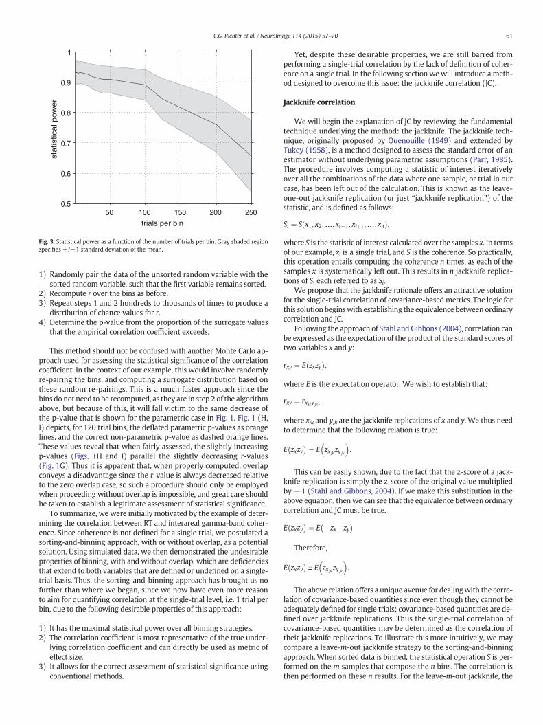
value. Fig. 1 reveals that the increase in the correlation coefficient ismir-rored by an increase in the p-value,which is simply explained by the de-crease in n (the number of bins) as the bin size increases. As aconsequence, with increasing bin size, more and more tests will fail toreach significance. We illustrate this with the power analysis shown inFig. 3. The curve in Fig. 3 corresponds to the zero-overlap tests shownby the blue curves in Figs. 1 and 2. Statistical power is the probabilityof correctly identifying an experimental effect, and thus quantifies thesensitivity of a test. To establish the statistical power as a function ofbin size we performed the following Monte-Carlo simulation (keepingthe type I error rate fixed at 0.05). We first simulated (using theMATLAB function mvnrnd) two random variables of sample size n andexpected correlation r, and computed the observed correlation r inthat sample. This was repeated 1000 times, leading to a randomizationdistribution for r. Second,we generated two randomvariables of samplesize n and correlation r of zero, and computed the correlation r0, again1000 times, leading to a randomization distribution for r0. From this lat-ter distribution, we determined the 95th percentile. Finally, we deter-mined the proportion of the randomization distribution of r thatexceeded the 95th percentile of the randomization distribution of r0.This proportionwas taken as the power for detecting a significant corre-lation, given r and n. For a true r of 0.1, Fig. 1A shows the estimates of r

50 100 150 200 2500
0.5
1
r
binned correlation
50 100 150 200 2500
0.05
0.1
trials per bin
p−va
lue
250 200 150 100 50
leave−m−out jackknife correlation
−250 −200 −150 −100 −50
trials left out = m
−4 −2 0 2
−2
0
2
Sorted rv
Uns
orte
d rv
5 10 x 10−3
0.034
0.036
0.038
Sorted rv
Uns
orte
d rv
−2 0 2
−0.2
0
0.2
0.4
Sorted rv
Uns
orte
d rv
−0.1 0 0.1
0.02
0.03
0.04
0.05
Sorted rv
Uns
orte
d rv
−1 0 1
−0.1
0
0.1
0.2
Sorted rv
Uns
orte
d rv
−0.2 0 0.2
0.02
0.04
0.06
Sorted rv
Uns
orte
d rv
−1 0 1−0.1
0
0.1
Sorted rv
Uns
orte
d rv
−0.4 0 0.4−0.02
0
0.02
0.04
0.06
0.08
Sorted rv
Uns
orte
d rv
A B
C D
E GF H
I KJ L
Fig. 2. Equivalence of binned correlation with leave-m-out jackknife correlation. A, B. Pearson's r as a function of bin size (A), and as a function of the number of trials left out (B). C, D.Corresponding p-values for panels A and B. E, F, I, J. Scatter plots of the bin averages of the sorted and unsorted random variables (rv) for the 4 correspondingly colored points shownin A and C. G, H, K, L. Scatter plots of the leave-m-out averages of the sorted and unsorted random variables (rv) for the 4 correspondingly colored points shown in B and D.
60 C.G. Richter et al. / NeuroImage 114 (2015) 57–70
for different overlap percentages and bin sizes. For zero overlap and arepresentative subset of bin sizes, we determined the number of binsn and the estimate of r (the latter by reading from Fig. 1A). For thosepairs of r and n, we determined the statistical power, as explainedabove, 100 times and show the average statistical power across those100 repetitions in Fig. 3.
As suspected based on the behavior of the p-value with increasingbin size, the statistical power systematically decreases as the bin sizeis increased from 1 trial to 250 trials. As bin size increases, the num-ber of bins decreases, thus though the correlation coefficientsincrease (Figs. 2E, F, I, and J), this increase is countered by a decreasein the number of observations, which results in a net loss of statisticalpower.
To summarize, the binning of data (even without overlap betweenbins), results in an increase in the correlation coefficient due to smooth-ing of the data, and a decrease in the statistical power of the test. Thusthis analysis indicates that the optimal approach is to not use a binningstrategy, such that statistical power ismaximized and the r and r2 valuescan directly be taken as metrics of effect size.
Let's now consider the effects of overlapping the bins. It is apparentfrom the r surfaces/lines in Figs. 1A, D, and G, that binning with overlapleads to the same inflation of the correlation coefficient that occurswithout overlap. It is also clear that overlapping the bins also leads toa marginal decrease in the r-value, but more worrisome is the massivedecrease in the p-value as overlap is increased. Following the coloredcurves (red, orange, yellow) in Figs. 1B, C, H, and I, we can see that thep-value dramatically decreases as overlap is increased. The result ap-pears attractive, since large r-values are achieved in combination withimpressively small p-values, but these results are false, because thedata points entered into the correlation analysis are not independentdue to the bin overlap. With an increasing degree of overlap, the binsbecome less independent, which effectively inflates the degrees of free-dom (df), such that from the point of view of the test, there are far moreobservations thanwere in fact there. This is basic statistics, but the issueshould be kept in mind since in more complex designs, this violationmay be more difficult to spot. If conditions demand that overlap mustbe used, the statistical inflation may be corrected by applying thefollowing Monte Carlo approach to computing the p-value:
50 100 150 200 2500.5
0.6
0.7
0.8
0.9
1st
atis
tica
l po
we
r
trials per bin
Fig. 3. Statistical power as a function of the number of trials per bin. Gray shaded regionspecifies +/−1 standard deviation of the mean.
61C.G. Richter et al. / NeuroImage 114 (2015) 57–70
1) Randomly pair the data of the unsorted random variable with thesorted random variable, such that the first variable remains sorted.
2) Recompute r over the bins as before.3) Repeat steps 1 and 2 hundreds to thousands of times to produce a
distribution of chance values for r.4) Determine the p-value from the proportion of the surrogate values
that the empirical correlation coefficient exceeds.
This method should not be confused with another Monte Carlo ap-proach used for assessing the statistical significance of the correlationcoefficient. In the context of our example, this would involve randomlyre-pairing the bins, and computing a surrogate distribution based onthese random re-pairings. This is a much faster approach since thebins do not need to be recomputed, as they are in step 2 of the algorithmabove, but because of this, it will fall victim to the same decrease ofthe p-value that is shown for the parametric case in Fig. 1. Fig. 1 (H,I) depicts, for 120 trial bins, the deflated parametric p-values as orangelines, and the correct non-parametric p-value as dashed orange lines.These values reveal that when fairly assessed, the slightly increasingp-values (Figs. 1H and I) parallel the slightly decreasing r-values(Fig. 1G). Thus it is apparent that, when properly computed, overlapconveys a disadvantage since the r-value is always decreased relativeto the zero overlap case, so such a procedure should only be employedwhen proceeding without overlap is impossible, and great care shouldbe taken to establish a legitimate assessment of statistical significance.
To summarize, we were initially motivated by the example of deter-mining the correlation between RT and interareal gamma-band coher-ence. Since coherence is not defined for a single trial, we postulated asorting-and-binning approach, with or without overlap, as a potentialsolution. Using simulated data, we then demonstrated the undesirableproperties of binning, with and without overlap, which are deficienciesthat extend to both variables that are defined or undefined on a single-trial basis. Thus, the sorting-and-binning approach has brought us nofurther than where we began, since we now have even more reasonto aim for quantifying correlation at the single-trial level, i.e. 1 trial perbin, due to the following desirable properties of this approach:
1) It has the maximal statistical power over all binning strategies.2) The correlation coefficient is most representative of the true under-
lying correlation coefficient and can directly be used as metric ofeffect size.
3) It allows for the correct assessment of statistical significance usingconventional methods.
Yet, despite these desirable properties, we are still barred fromperforming a single-trial correlation by the lack of definition of coher-ence on a single trial. In the following section wewill introduce a meth-od designed to overcome this issue: the jackknife correlation (JC).
Jackknife correlation
We will begin the explanation of JC by reviewing the fundamentaltechnique underlying the method: the jackknife. The jackknife tech-nique, originally proposed by Quenouille (1949) and extended byTukey (1958), is a method designed to assess the standard error of anestimator without underlying parametric assumptions (Parr, 1985).The procedure involves computing a statistic of interest iterativelyover all the combinations of the data where one sample, or trial in ourcase, has been left out of the calculation. This is known as the leave-one-out jackknife replication (or just “jackknife replication”) of thestatistic, and is defined as follows:
Si ¼ S x1; x2;…; xi−1; xiþ1;…; xnð Þ;
where S is the statistic of interest calculated over the samples x. In termsof our example, xi is a single trial, and S is the coherence. So practically,this operation entails computing the coherence n times, as each of thesamples x is systematically left out. This results in n jackknife replica-tions of S, each referred to as Si.
We propose that the jackknife rationale offers an attractive solutionfor the single-trial correlation of covariance-basedmetrics. The logic forthis solution beginswith establishing the equivalence between ordinarycorrelation and JC.
Following the approach of Stahl and Gibbons (2004), correlation canbe expressed as the expectation of the product of the standard scores oftwo variables x and y:
rxy ¼ E zxzy� �
;
where E is the expectation operator. We wish to establish that:
rxy ¼ rx jky jk;
where xjk and yjk are the jackknife replications of x and y. We thus needto determine that the following relation is true:
E zxzy� � ¼ E zx jk zy jk
� �:
This can be easily shown, due to the fact that the z-score of a jack-knife replication is simply the z-score of the original value multipliedby −1 (Stahl and Gibbons, 2004). If we make this substitution in theabove equation, thenwe can see that the equivalence between ordinarycorrelation and JC must be true.
E zxzy� � ¼ E −zx−zy
� �
Therefore,
E zxzy� �
≡ E zx jk zy jk
� �:
The above relation offers a unique avenue for dealingwith the corre-lation of covariance-based quantities since even though they cannot beadequately defined for single trials; covariance-based quantities are de-fined over jackknife replications. Thus the single-trial correlation ofcovariance-based quantities may be determined as the correlation oftheir jackknife replications. To illustrate this more intuitively, we maycompare a leave-m-out jackknife strategy to the sorting-and-binningapproach.When sorted data is binned, the statistical operation S is per-formed on the m samples that compose the n bins. The correlation isthen performed on these n results. For the leave-m-out jackknife, the

62 C.G. Richter et al. / NeuroImage 114 (2015) 57–70
correlation is performed on the n results of the function S applied to thedata remaining after each bin ofm trials has been left out once. The sym-metry of thesemethods is apparent in Figs. 2A–D, where leave-m-out JChas been applied to the numerical data used to investigate the conse-quences of sorting-and-binning, i.e. data forwhich single-trial estimatesare available. Figs. 2A–D show the comparison of correlations based onbinning without overlap (Figs. 2A and C), and leave-m-out JC (Figs. 2Band D). What is immediately obvious from the topmost panels is thatthe correlation functions are mirror symmetric. Comparison of the left-most point of the binned correlation (Figs. 2A and C), corresponding to abin size of 1; with the rightmost point of the leave-m-out JC (Figs. 2Band D), which corresponds to the leave-one-out JC, reveals preciselythe same r-values and p-values. Thus, as dictated by the mathematicalproof, conventional correlation is equivalent to JC.
JC has a particular strength that should be noted. Since the methoddoes not require the sorting of any variables, neither variable involvedin the correlation needs to be defined on a single-trial basis. Thismeans that the method may be used to assess the correlation betweentwo variables that are both not defined on the level of a single trial.
Note that the JC entails an inversion and compression of the sampledistributions by the jackknife method. This can be seen by comparingthe binned versus the leave-m-out jackknife scatter plots in Figs. 2E–L.The leave-m-out jackknife scatter plots are up/down and left/right mir-ror reversals of the scatter plots that result from binning. Furthermore,the JC scatter plots contain smaller values, because they essentially rep-resent only the small changes in the function Fwhen a single trial out of1000 trials is left out. Both the compression and the double inversion areirrelevant for correlation analysis. The compression is compensated bythe fact that the correlation coefficient normalizes the covariance bythe product of the variances of each of the two variables. The inversionis irrelevant, because it occurs in both variables, and correlation is in-variant to the sequence of the paired variables. Yet, if instead of linearcorrelationmetrics, non-linearfits are to be performed, or non-linear ef-fects are qualitatively assessed visually from the data, onemust be care-ful to provide the correct interpretation. To illustrate this point, Fig. 4shows the effect of the JC for two example variables with a non-linearrelation. This makes the inversion very apparent and the potential formisinterpretation quite obvious.
It must also be noted that the jackknife technique in general, andthereby also the JC, should only be used in combination with statisticswhose underlying distributions are smooth (Miller, 1974; Efron, 1979;Parr, 1985). An example of a statistic that is not smooth is the median.The jackknife replications of themedian of a distribution are themiddletwo values of the distribution. These two values do not capture the var-iance contained in the full distribution, which we attempt to capture
0.2 0.4 0.6 0.8
0.20.40.60.8
rv 1
rv 2
0.5015 0.502 0.5025 0.503
0.1985
0.199
0.1995
0.2
rv 1 (leave−1−out)
rv 2
(le
ave−
1−ou
t)
Fig. 4. The jackknife procedure causes an inversion of the distribution and a variancecompression of random variable 1 (rv1) and random variable 2 (rv2).
with the jackknife method. Most functional connectivity metrics, suchas coherence, are based on an averaging operation over the trial dimen-sion, and thus should be suitable for use with the JC.
Numerical investigation of JC and application to simulated data:methods
Wehave demonstrated in Fig. 2 that, for parameters that are definedon a single trial, the JC is identical to the conventional single-trial corre-lation. Ideally, we would want to show that the same holds for metricsof interactions like coherence. Yet, this is problematic since the coher-ence is not defined for single spectral estimates, and therefore, the JCfor coherence cannot be compared against a ground-truth estimate.While we cannot estimate coherence for single spectral estimates, wemay generate simulated data epochs with a coherence that is propor-tional to a coupling parameter c using a generative model (Brovelli,2012). If we further vary c across multiple instantiations of this genera-tive model, we can expect that c will be correlated with the single-trialcoherence. We employ such a setup to test whether trial-by-trial corre-lation generated in this way can be recovered by the JC technique.
We constructed the following autoregressive (AR) model to gener-ate appropriate data to test the JC technique in a system exhibitinginter-areal coherence and unidirectional GC:
xt ¼ 0:95xt−1−0:8xt−2 þ εx;tyt ¼ 0:8yt−1−0:5yt−2 þ cxt−1 þ εy;t ;
where xt and yt represent time series from two brain areas. xt is a func-tion of its own values at one and two time steps in the past, i.e. xt − 1 andxt − 2, weighted by some chosen coefficients (0.95 and −0.8), plus εx,t,i.e. an noise term (also called the innovation). The situation is similarfor yt, except that it is a function not only of its own past values plusthe noise term, but also of yt − 1, weighted by c. This model is a bivariate(two signals) autoregressive (the signals depend on their own past)model of order two (they depend on two time steps into the past), i.e.it is an AR(2) model. We chose an AR(2) model specifically, because itis the model of minimal complexity that generates synthetic data withband limited power, coherence, and GC spectra. The crucial aspect ofthe model is that it exhibits unidirectional coupling and thereby coher-ence that is determined by the parameter c. This will allow us to vary cfrom trial to trial and thereby generate fluctuations in coherence thatare perfectly rank-correlated with the fluctuations in c. While c mighttranslate into the coherence magnitude in a non-linear way, it doestranslate in a monotonic and smooth way and this guarantees that theexpected rank correlation has a value of one. Fifty time-series pairswere generated for the bivariate AR(2) process with each time-seriesmodulated by a unique coupling parameter value c chosen randomlyfrom a uniform distribution between 0 and 0.1. Each time series was25,600 samples long at a sampling rate of 500 Hz, resulting in51.2 second segments. AR models cannot only generate simulatedtime series, but they can also be fit to experimental or to simulateddata in order to quantify the spectral properties, like power, coherenceor GC. For all parametric analyses of the generated data, AR modelingwas performed using software developed by Steven Bressler andMingzhou Ding. The model parameters were determined using avectorized implementation of the algorithmofMorf et al. (1978), gener-ously provided by Anil Seth and Lionel Barnett (Barnett and Seth, 2014).Bivariate AR(2) models were fit to the synthetic time-series pairs usingportions of the data truncated to varying lengths (see Fig. 6). In the caseof conventional single-trial correlation,models were fit to the data fromeach trial pair, while in the case of JC, models were fit using all trialsminus one for all leave-one-out possibilities. Coherence and Grangercausality spectra (Granger, 1969; Geweke, 1982) were derived fromthe fitted AR(2) models, and the max of the spectrum was selected.For these max values we then determined their correlation with thecoupling coefficient c. This procedure was repeated 1000 times with

63C.G. Richter et al. / NeuroImage 114 (2015) 57–70
the mean taken over the resulting ensemble of Spearman's rho correla-tion coefficients to achieve sufficiently smooth estimates. All p-valueswere determined parametrically.
Spectral estimates were also obtained using non-parametric analy-sis. All non-parametric spectral connectivity analyses were performedusing Fieldtrip (Oostenveld, et al., 2011). Spectral estimates werecomputed via a Fourier transform using the multi-taper method(Mitra and Pesaran, 1999; Thomson, 1982) with a spectral smoothingof +/−10 Hz. We compared the JC approach to a non-JC approachbased on epoch subdivision of single trials. In the subdivision-based ap-proach, for data windows less than 400 ms in length, the cross-spectraldensity (CSD) was computed as the mean of the estimates derivingfrom the multiple data tapers. For trial lengths longer than 400 ms,400 ms windows with 300 ms overlap were employed. In these cases,the CSD was computed as the mean over tapers and windows. For theJC-based approach, the CSD was determined via jackknifing, which en-tails taking the mean CSD resulting from all trials minus one, for eachwindow, for all leave-one-out combinations. Coherence spectra werederived from the power and CSD, while GC spectra were determinedusing non-parametric spectral factorization, which is a method ofobtaining GC from non-parametric spectral estimates such as the Fouri-er or wavelet transform (Dhamala et al., 2008a,b; Wilson, 1972). Thisprocedure was performed for each 400 ms window and followingWelch'smethod (1967) the coherence andGC spectra for each jackknifereplicationwere determined as the average over thewindows. The peakvalue of the coherence andGC spectrawas determined, and themean ofthe frequency band of +/−30 Hz around this peak was used for subse-quent JC and conventional single-trial correlations. As for the parametriccase, this procedure was repeated 1000 times to achieve smooth esti-mates of Spearman's rho and parametrically determined p-values.
Numerical investigation of JC and application to simulated data:results
We fit an AR(2) model to the first 10 s of the simulated data toinspect the spectral properties of the simulated data (Fig. 5). The useof a long 10-second segment allows us to capture the parameters of
0 50 100 1500
0.1
0.2
pow
er
0 50 100 1500
0.02
0.04
0 50 100 150 0 50 100 150
0 50 100 1500
0.2
0.4
cohe
renc
e
0
0.05
0.1
0
0.2
0.4
0
0.2
0.4
c-pa
ram
eter
GC
frequency
frequency (Hz) frequency (Hz)
frequency (Hz) frequency (Hz)
xt yt xt yt
xt yt
ytxtA B
C
D E
Fig. 5. Spectral properties of the bivariate autoregressive model for various values of thecoupling parameter c. A. Power of variable Xt for the 50 simulated time series. B. Powerof variable Yt for the 50 simulated time series. C coherence between Xt and Yt for the 50simulated time series. D. Granger causality of Xt to Yt for the 50 simulated time series. E.Granger causality of Yt to Xt for the 50 simulated time series. Colorbar denotes the magni-tude of the coupling coefficient c.
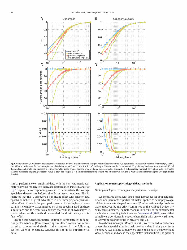
themodel almost perfectly, and clearly see the effects ofmodulating pa-rameter c. It is apparent that in all spectra, where there is spectral ener-gy, that there is a peak between 70 and 90 Hz, corresponding to thegamma band, as specified by the model parameters. It is also apparentthat the single-trial power of xt (Fig. 5A) is not modulated by c, whichis evident since the progression of color from the smallest to largestpeak does not follow the color scheme corresponding to parameter c,whereas the power of yt (Fig. 5B), though lower in overall value,shows modulation by c based on the color progression. This is due tothe unidirectional flow of power from xt to yt that is modulated by c.The coherence shown in Fig. 5C shows clear modulation by c, and theGC (Figs. 5D and E) shows unidirectional coupling also modulated byc. We determined the JC between c and coherence or GC influence andconfirmed that it approaches a value of one for long epoch lengths(Fig. 6A for coherence, B for GC influence). These JCs are shown inblue for spectral estimates derived from fitting AR models, and in goldfor spectral estimates derived non-parametrically. For shorter epochlengths, the JC decays. Short epochs realize the properties of the gener-ative model only in an imperfect way. Thus, the decay in JC correlationaway from the value of one is not necessarily due to an imperfect esti-mation of the underlying correlation, but it is likely due to the factthat the correlation between, on the one hand c, and on the otherhand the short-epoch coherence is actually low. In order to substantiatethis claim,we turn again to a case inwhichwe can quantify themetric ofinterest on data epochs of arbitrary length. We generated 50 Gaussianrandom signalswith zeromean and unit variance.We then added a ran-dom offset o to each of these signals, drawn from a uniform randomdis-tribution between zero and one. We then correlated the o to the meanscalculated over data epochs of variable length (randomly subsampledfrom the full-length signal). The result is shown in Fig. 7. As the dataepochs get shorter, the correlation between the epochs' means andthe values of r falls off in a way that is very similar to the drop-off in cor-relation seen in Fig. 6. This effect is solely due to error between the sub-sample means and the original offsets (which are equal to the full-length data means). Thus, this is not due to an error in estimating themean, but rather it is due to the failure of the shorter data segment toexpress the expected mean of the process. With this in mind, we cango back to Fig. 6. With the imperfect expression of the model parame-ters in short epochs explaining an overall drop-off, we can turn to thedifferences between different approaches to estimating the correlationbetween short epochs across single trials. In Figs. 6A and B, we seethat indeed as the trial length decreases, so does the correlation coeffi-cient. The critical test for JC is to determine if, for a given epoch length,themethod is providing superior estimates of the correlation coefficientin comparison to conventional approaches to this problem.We comparethe JC against conventional single-trial correlations, which attempt toestimate the Fourier transform from single, short data epochs using ei-ther overlapping data windows (Fig. 6, green lines) or single-trialAR(2)models (Fig. 6, red lines). We see in Figs. 6A and B that at the lon-gest epoch length, the correlation coefficient based on either conven-tional single-trial metrics approached one, like the JC correlations.Critically, as the epoch length decreased, the JC estimates of the correla-tion coefficients remained above the correlation coefficients based onsingle trial parametric estimates (Fig. 6, red lines) and non-parametricestimates (Fig. 6, green lines). This is even more evident if we plot thepercentage difference between the estimator with the largest correla-tion coefficient at each trial length and each of the different metrics, asshown in Figs. 6C and D, where we see similar performance betweenthe JC on parametrically and non-parametrically derived estimatorswhen the trial length exceeds 300ms. The small superiority of paramet-ric JC versus non-parametric JC, particularly for shortwindow lengths, islikely due to two effects: 1) data windowing effects in the non-parametric approach, which are exacerbated at short epoch lengthsand 2) the fact that the data had been generated with a parametricmodel and therefore might be fitted particularly well with a parametricmodel. As will be shown in the following section, both metrics show
102
103
104
0
0.2
0.4
0.6
0.8
1Granger Causality
102
103
104
102
103
104
0
0.02
0.04
0.06
0.08
0.1
trial length (ms)
102
103
104
0
0.2
0.4
0.6
0.8
1
rho
Coherence
102
103
104
100
80
60
40
20
0
102
103
104
0
0.02
0.04
0.06
0.08
0.1
p−va
lue
trial length (ms)
A B
C D
E F
% s
mal
ler
than
bes
t est
imat
e
100
80
60
40
20
0
parameric JCnon-parameric JCparameric single-trialnon-parameric single-trial
Fig. 6. Comparison of JCwith conventional spectral correlationmethods as a function of trial length on simulated time series. A, B. Spearman's rank correlation of the coherence (A) andGC(B), with the coefficient c for the 50 coupled simulated time series Xt and Yt as a function of trial length. Blue squares depict parametric JC, gold triangles depict non-parametric JC, reddiamonds depict single-trial parametric estimation, while green crosses depict a window-based non-parametric approach. C, D. Percentage that each correlation metric is smallerthan the metric yielding the greatest rho-value at each trial length. E, F. p-Values corresponding to each rho-value shown in A and B with dashed lines marking the 0.05 significancethreshold.
64 C.G. Richter et al. / NeuroImage 114 (2015) 57–70
similar performance on empirical data, with the non-parametric esti-mator showing moderately increased performance. Panels E and F ofFig. 6 display the corresponding p-values to demonstrate the averageepoch length necessary before a significant result is obtained. This il-lustrates that the JC discovers a significant effect with shorter dataepochs, which is of great advantage in neuroimaging analysis. An-other effect of note is the poor performance of the single-trial non-parametric window-based method on short epochs. Based on thesesimulations and the empirical analyses that will be shown below, itis advisable that this method be avoided for short data epochs infavor of JC.
In conclusion, these numerical examples demonstrate the supe-rior performance of JC in recovering simulated correlations com-pared to conventional single trial estimates. In the followingsection, we will investigate whether this holds for experimentaldata.
Application to neurophysiological data: methods
Electrophysiological recordings and experimental paradigm
We compared the JC with single-trial approaches for both paramet-ric and non-parametric spectral estimators applied to neurophysiologi-cal data to evaluate the performance of JC. All experimental procedureswere approved by the ethics committee of the Radboud UniversityNijmegen (Nijmegen, The Netherlands). For details of the experimentalmethods and recording techniques see Bosman et al. (2012), except thatstimuli were positioned in opposite hemifields with only one stimulusco-activating recording sites in areas V1 and V4.
Two rhesus monkeys (Macaca mulatta) were trained to perform acovert visual spatial attention task. We show data in this paper frommonkey K. Two grating stimuli were presented, one in the lower rightvisual hemifield, and one in the upper left visual hemifield. The gratings

100
101
102
103
0
0.2
0.4
0.6
0.8
1
length (samples)
r
Fig. 7. The effect of trial length (samples) on the correlation (r) between twoperfectly cor-related random variables.
65C.G. Richter et al. / NeuroImage 114 (2015) 57–70
were isoluminant and iso-eccentric drifting sinusoidal gratings with adiameter of 3° visual angle, a spatial frequency of 0.66 cycles/degree,drift velocity of 1.2°/s, with a resulting temporal frequency of 0.8 -cycles/s and 100% contrast. The two gratings had orientations thatwere always 90° away from each other and, when they were moving,inconsistent with the interpretation of a chevron pattern seen throughtwo apertures. For a given session, two orientations were chosen, andon a given trial, the orientation shown contralateral to the ECoG gridwas chosen from those two orientations pseudorandomly. The stimuliwere presented on a CRT monitor with a 120 Hz refresh rate non-interlaced. For each trial, one stimulus was randomly tinted yellow,and the other blue. Local field potentials (LFP) were recorded from theleft hemisphere with a subdural electrocorticographic (ECoG) gridconsisting of 252 electrodes (1 mm diameter), spaced 2–3 mm apart.Signals from immediately neighboring electrodeswere subtracted to re-move the common recording reference, because otherwise the commonreference leads to artifactual coherence/GC influence. We refer to thebipolar derivative resulting from the subtraction of two neighboringelectrodes as a “site”. For coherence andGC influence analysis,we inves-tigated interactions between primary visual cortex (V1) and extrastriatevisual cortex (V4). The assignment of electrodes to brain areas wasbased on macaque brain atlases. The current analysis examined 29sites recorded from area V1 and 17 sites recorded from area V4,resulting in 493 V1–V4 site pairs.
The covert spatial attention task consisted of three successiveepochs. 1) The prestimulus period where the monkey had achieved fix-ation. 2) The pre-cue period where the stimulus gratings had appearedand themonkeywaited for a color cue, and 3) the cue period, where thefixation point changed color to indicate to which stimulus the monkeyshould attend, and respond to (the target).While the stimuli were pres-ent, either the target or distractor could change shape at any time. Themonkey was rewarded for responses to a change of the shape of targetstimulus.
For the examples presented in this paper, trials were selected fromdata segments that spanned at least 2 s from cue onset prior to any stim-ulus change. The first 0.4 s of this segmentwere discarded to avoid tran-sients generated by the cue change, leaving 1.6 s for analysis.Correlations were then assessed for 8 different pairs of data windowsof varying length from 0.1–0.8 s. Each pair consisted of an early andlate segment such that the early windows always terminated one sam-ple prior to 1.2 s, whereas the later windows always commenced at1.2 s. 352 trials were selected from 9 sessions. Trials were included
where attention was directed to either visual hemifield, i.e. data werepooled across attention conditions.
Spectral estimation
The spectral properties of the data were determined both paramet-rically via AR modeling, and non-parametrically via Fourier analysis sothe performance of JC could be compared for both techniques. Paramet-ric spectral estimates were computed in the following way. Data wasresampled to 250Hz. The coherence, and Granger Causal (GC) influencein the “bottom-up” direction (V1 to V4) were then obtained by fittingbivariate autoregressive (AR) models with model order 9, computedfor each V1–V4 pair of sites. The model order was determined via theminimaof the Bayesian Information Criterion (BIC) andAkaike Informa-tion Criterion (AIC), between model orders 1 and 25. When the modelwas used for more than one data epoch, e.g. for JC on all-but-one trial,the fit was simultaneously to the ensemble of epochs (Ding et al.,2000), where a separate model was constructed for each leave-one-out jackknife replication. For the non-parametric JC analyses, Fouriertransforms were computed using the multi-taper method (Mitra andPesaran, 1999; Thomson, 1982) on de-meaned data segments with+/−10Hz smoothing. For the JC approach, all thedata segments (8 var-iable lengths from0.1–0.8 s)were zero-padded to 1 s, resulting in a con-sistent 1 Hz spectral grid, with the CSD for each jackknife replicationderived as the mean CSD over trials after one trial had been left out.Spectral coherence was computed for each jackknife replication, whileGC was determined via non-parametric spectral factorization of eachreplication. Identical to theparametricmethod, coherencewas analyzedbetween V1 and V4 channels and the “bottom-up” direction was ana-lyzed from V1 to V4 for the GC. The single-trial approach followed thatof Brovelli (2012), where a 250 ms window (zero-padded to 1 s), wasmoved at 5 ms steps throughout each single trial, to construct multipleestimates of the CSD, where coherence and GC were determined fromthe average of these CSD estimates. To ensure that at least ten CSD esti-mates were averaged before computing coherence or GC, only trialswith lengths of at least 300 ms were analyzed.
A standardized peak frequencywas employed for all analyses whereactivitywas assessed at a single spectralmaximum. To establish this, co-herence and GC were estimated over the entire 1.6 s of data. This wasdone for both parametric and non-parametric implementations. AHann taper was used for the non-parametric estimation, otherwise allthe spectral estimation parameters were identical to those outlinedabove. The peak GC and coherence were found to lie in the gammaband at 74 Hz for the parametrically derived estimates and 75 Hz forthe non-parametric technique, whichwere subsequently used through-out, for the parametric and non-parametric analyses, respectively.
Statistical analysis
We determined the correlation between coherence (or GC influ-ence) from two neighboring within-trial epochs, across trials, for eachfrequency–frequency combination. Correlations were computed eitherbetween conventional single-trial estimates or using the JC. This wasdone for all frequency–frequency combinations between 51 and100 Hz. For the assessment of statistical significance of correlations, aMonte Carlo approach was employed andwas identical for both the co-herence and GC, and parametric and non-parametric cases. The test sta-tistic used was the mean Spearman's rho computed over the jackknifereplications from the early and late epochs for all the possible V1–V4pairs. To construct the surrogate distribution, the JC between the earlyand late epochs was determined after the jackknife replications hadbeen randomly paired, i.e. the trial order of the early epoch was ran-domized with respect to the late. Note that the random trial reorderingwas identical for each V1–V4 site pair. This was repeated 1000 times toform a null distribution ofmean Spearman's rho values,which functions

66 C.G. Richter et al. / NeuroImage 114 (2015) 57–70
to disrupt the empirical relationship between the early and late epochsingle trial pairs, so that their empirical degree of correlation can becomparedwith the distribution of correlation coefficients that occurreddue to chance. When we computed JC on eight neighboring windowsranging from 0.1 to 0.8 s, this procedure was repeated for each of theeight epoch lengths, resulting in eight null distributions. When testingfor cross-frequency interactions, the issue of multiple comparisonsneeded to be addressed. To correct for the multiple comparisons overthe 50 × 50 frequency combinations, the largest absolute value of thecorrelation across all frequency–frequency combinations was selectedfor each of the 1000permutations, resulting in a distribution ofmaximaltest statistics (Nichols and Holmes, 2002). Empirical test statistic valueswere considered significant at p = 0.05, two-tailed, if their absolutevalue was larger than the 975th percentile of the distribution. Wherep-values smaller than 0.05 are shown for visualization purposes, thetail of the distribution above the 975th value was extrapolated with aGeneralized Pareto distribution function, an appropriate distributionfor modeling the extreme values of a distribution.
A parametric approach was used to assess the statistical significanceof a representative single channel pair over the eight neighboringepochs. Here we wished to show the precise p-value that correspondedwith each rho-value, whichwas not feasible using a non-parametric ap-proach since the p-values are sufficiently small that a Monte Carlomethod is not computationally tractable to estimate these values. Weused the standard approach, where the rho-value and number of trialsare used to derive a t-statistic, which in combination with the corre-sponding degrees of freedom yields the p-value from Student'st-distribution (Rahman, 1968).
100 200 300 400 500 600 700 800
mea
n rh
o
Coherence
100
80
60
40
20
0
trial length (ms)
% s
mal
ler
than
bes
t est
imat
e
100 200 300 400 500 600 700 800
A B
C D
parameric JCnon-parameric JCparameric single-trialnon-parameric single-trial
−0.05
0
0.05
0.1
0.15
Fig. 8. Comparison of JC with conventional spectral correlation methods as a function of trial lebottom-up GC (B) between two neighboring time windows, averaged over V1–V4 site pairs. Tmean rho-value at which the statistical significance is 0.05, with each color corresponding tothan themetric yielding the greatest rho-value at each trial length. Gold triangles depict non-paestimation, while green crosses depict a window-based non-parametric approach.
Application to neurophysiological data: results
Bosman et al. (2012) have established that areas V1 and V4 showrobust gamma band coherence and bottom-up GC during sustainedattention. It is well known that the correlation between neighboringtime-points in a trial dissipates as the temporal distance betweenthem increases (autocorrelation). We capitalize on this property tocompare JC with single-trial methods for both parametric and non-parametric spectral estimators of the strength of V1–V4 gamma coher-ence and bottom-up GC influence. The logic is that neighboringwindows should show correlated coherence and GC, which we can as-sess using JC. To achieve this, we calculated the correlation betweenthe magnitude of gamma band coherence (and bottom-up GC influ-ence) from two neighboringwithin-trial analysis windows, across trials.Fig. 8 shows the same characteristic pattern that resulted from the nu-merical simulations (Fig. 7), where the correlation coefficients increaseas the data window is increased in length. Asmentioned above, the twodata windows were neighboring within a given trial, and one mighttherefore be concerned that longer windows included data temporallymore adjacent, and therefore more correlated. To counter this potentialeffect, the windows were designed such that the end point of the firstwindow coincided with the starting point of the second window,which results in longer windows possessing data that are temporallymore distant. In agreement with the simulations, the JC curves for theaverage over all V1–V4 site pairs (Figs. 8A and B, parametric: bluelines, non-parametric gold lines) show a considerable improvementover conventional single trial approaches (Figs. 8A and B, parametric:red line, non-parametric: green lines). Fig. 9 shows an example V1–V4
100 200 300 400 500 600 700 800
Granger Causality
trial length (ms)
100
80
60
40
20
0
100 200 300 400 500 600 700 800
−0.05
0
0.05
0.1
0.15
ngth for V1–V4 channel pairs. A, B. Spearman's rank correlation of the coherence (A) andhe shaded area indicates the standard error of the mean (s.e.m). Dashed lines denote thethe respective correlation metric. C, D. Percentage that each correlation metric is smallerrametric JC, blue squares depict parametric JC, red diamonds depict single-trial parametric

−0.2
0
0.2
0.4
0.6Granger Causaility
−0.2
0
0.2
0.4
0.6Coherence
10−20
10−10
100
p−va
lue
trial length (ms)100 200 300 400 500 600 700 800
trial length (ms)100 200 300 400 500 600 700 800
10−20
10−10
100
200
160
120
80
40
0
rho
100 200 300 400 500 600 700 800200
160
120
80
40
0
100 200 300 400 500 600 700 800
100 200 300 400 500 600 700 800 100 200 300 400 500 600 700 800
A B
C D
E F
% s
mal
ler
than
bes
t est
imat
e
parameric JCnon-parameric JCparameric single-trialnon-parameric single-trial
Fig. 9. Comparison of JC with conventional spectral correlation methods as a function of trial length for a selected V1–V4 channel pair. A, B. Spearman's rank correlation of the coherence(A) and bottom-up GC (B) between two neighboring timewindows for a selected V1 channel and V4 channel pair. C, D. Percentage that each correlationmetric is smaller than themetricyielding the greatest rho-value at each trial length. E, F. p-Values corresponding to each rho-value shown inA andB.Gold triangles depict non-parametric JC, blue squares depict parametricJC, red diamonds depict single-trial parametric estimation, while green crosses depict a window-based non-parametric approach.
67C.G. Richter et al. / NeuroImage 114 (2015) 57–70
pair of sites employing the same plotting conventions a Fig. 6. As in thegroup average, the JC correlation curves (Figs. 9A and B) show amarkedincrease over the conventional single-trial approaches. Figs. 9E and F re-veal that JC ismuchmore sensitive for revealing correlations.While con-ventional correlation approaches do not reach significance, JC issignificant forwindow lengths of 200ms and beyond, for both coherenceand GC influence. These results demonstrate that for biologically/behav-iorally interesting window lengths, the JC method substantially outper-forms conventional approaches. It is also apparent that the parametricand non-parametric JC approaches provide similar results. Parametric JCwas slightly superior for coherence on the shortest windows. Non-parametric JC was slightly superior for coherence at all other windowlengths and considerably superior for GC at all window lengths (Fig. 8D).
For the shortest data window of 100 ms, we now apply the JC ap-proach for all frequency–frequency combinations. Fig. 10 reveals
significant correlation of the coherence for a range of frequenciessurrounding the gamma band peak, both when determined non-parametrically (Fig. 10A) and parametrically (Fig. 10C). The precisespectral extent of the peaks is due to the specific choices of the para-metric and non-parametric spectral estimation, i.e. the model orderand the number of data tapers. The JCs of GC (Fig. 10B for non-parametric JC and D for parametric JC) show similar results.Fig. 10E shows a small significant region for parametrically deter-mined single-trial coherence, while Fig. 10F shows no significantcross-frequency correlation for single-trial parametric estimates ofGC, consistent with the numerical simulations (Fig. 6) and single-frequency analyses (Figs. 8 and 9).
Taken together, the empirical results demonstrate that over allwindow lengths tested, JC substantially outperforms conventionalsingle-trial methods.

frequency (Hz)
Granger CausailityCoherence
0.6
0.7
0.8
0.6
0.7
0.8
mea
n rh
o
p−va
lue
0.6
0.8
0.6
0.8
frequency (Hz)
mea
n rh
o
0
p−va
lue
0 0.0050.01
00.0050.01
mea
n rh
o
p−va
lue
0 0.0050.01
00.0050.01
mea
n rh
o
p−va
lue
6070
8090
1000 0.050.1
frequency (Hz)
60 70 80 90 10000.050.1
mea
n rh
o
p−va
lue
0 0.050.1
00.050.1
mea
n rh
o
p−va
lue
6070
8090
100
60 70 80 90 100
6070
8090
100frequency (H
z)
60 70 80 90 100
6070
8090
100
60 70 80 90 100
6070
8090
100
60 70 80 90 100
6070
8090
100
60 70 80 90 100frequency (Hz)
−0.025
−0.02
−0.015
−0.01
−0.005
0
0.005
0.01
0.015
0.02
0.025
−0.025
−0.02
−0.015
−0.01
−0.005
0
0.005
0.01
0.015
0.02
0.025
−0.025
−0.02
−0.015
−0.01
−0.005
0
0.005
0.01
0.015
0.02
0.025
−0.025
−0.02
−0.015
−0.01
−0.005
0
0.005
0.01
0.015
0.02
0.025
−0.025
−0.02
−0.015
−0.01
−0.005
0
0.005
0.01
0.015
0.02
0.025
−0.025
−0.02
−0.015
−0.01
−0.005
0
0.005
0.01
0.015
0.02
0.025
5e-2
5e-5
5e-5
5e-2
0
5e-5
5e-2
5e-5
5e-2
0
5e-5
5e-2
5e-5
5e-2
0
5e-5
5e-2
5e-5
5e-2
0
5e-5
5e-2
5e-55e-2
0
5e-4
5e-2
5e-2
5e-3
5e-4
5e-3
5e-4
5e-4
B
C D
E F
A
Fig. 10. Average correlation between two 100 ms neighboring windows over all V1–V4 pairs. A, B. Mean JC for coherence (A) and GC (B) computed from non-parametric estimates. C, D.Mean JC for coherence (C) and GC (D) computed from parametric spectral estimates. E, F. Conventional correlation computed from parametric single-trial estimates. For each panel (A–F),the central plot depicts themean correlation over channel pairs for each frequency–frequency combination,with different shadings reflecting p-values of 0.01, 0.001, 0.0001, and 0.00001.Contour lines correspondwith shading transitions, with the gray-scale value corresponding to the p-value, wherewhite indicates the lowest p-value and black the largest. Spectral plots tothe left of the frequency–frequencymap correspond to the average spectrum over V1–V4 pairs of the earlier time window, while spectral plots below themap correspond to the averagespectrumof the later timewindow. Colorbars indicate themean correlation over pairs and the corresponding p-values, with shading and gray-scale lines following the same convention asthe shaded areas and contour lines of the frequency–frequency maps.
68 C.G. Richter et al. / NeuroImage 114 (2015) 57–70
Discussion
To summarize, we presented jackknife correlation (JC) that allowsthe relation of moment-by-moment fluctuations in correlation strengthto other parameters, even though either correlation metric may not bedefined on a moment-by-moment basis, i.e. on the basis of a single
observation. We started out by investigating an approach that hasbeen commonly used in the case of assessing correlation between asingle-trial defined variable and an undefined variable, namely thesorting-and-binning approach. In this case, the single-observation-defined variable allows the sorting-and-binning, which in turn allowsthe calculation of the single-observation-undefined metric over the

69C.G. Richter et al. / NeuroImage 114 (2015) 57–70
multiple observations in each bin. The sorting-and-binning approach isoften used with overlapping bins in order to copewith limited numbersof observations. We demonstrated that the sorting-and-binning ap-proach leads to correlation coefficients that depend on the choice ofbin size and bin overlap and therefore can only be interpreted withthese parameters in mind, which makes them difficult to compareacross studies. Furthermore, we found that statistical powerwas actual-ly maximal when correlations were determined across single observa-tions, rather than across binned data. Since sorting-and-binning maybe considered a form of factorial design, where bin is considered a fac-tor, our numerical results support the arguments presented by Stahland Gibbons (2004), that the correlative framework is indeed themore powerful approach. Moreover, when overlapping bins are used,a failure to control for the lack of independence between bins can leadto erroneous p-values with a dramatic overestimation of statistical sig-nificance. These difficulties and insights motivated the introduction ofJC, which was shown to optimally address the above concerns.
The JC not only provides a quantitative improvement of estimationproperties in comparison to the sorting-and-binning approach, butmost critically, it allows for the extension of correlation to cases whereneither variable is defined on the level of a single trial. While thesorting-and-binning approach always requires that one of the correlat-ed variables be defined for single observations, the JC does not requirethis and therefore allows determination of the correlation betweentwo single-observation-undefined metrics. This allows, for example,the investigation of whether the functional connectivity betweenbrain areas A and B depends on the functional connectivity betweenbrain areas C and D.
In the same vein, we note that the scope of the JC reaches beyond re-latingfluctuations in correlation strength. The JC can facilitate the inves-tigation of relations for any metric that is defined only across multipleobservations (or observation epochs) and that is a smooth function ofthe observations (i.e. leaving out one of many observations results in acorrespondingly small change). For example, the variance is a smoothfunction that is defined only across multiple observations. The JC pro-vides a straightforward approach to relating e.g. fluctuations in neuro-nal response variance to stimulus or task parameters, or even relatingfluctuations in neuronal response variances between different brainareas. Additionally, use of the JC is not limited to electrophysiologicaldata, but is equally applicable to all time-series analyses, such as thatused in fMRI or in fields outside of neuroscience.
Here, we were particularly interested in frequency-resolved, i.e.spectral, analyses. The estimation of any spectral estimator, in order todefine frequency, requiresmultiple observations to form an observationepoch of finite length. The epoch length in turn defines the frequencyresolution of the spectral estimator. Spectrally resolvedmetrics of corre-lation, like coherence, when estimated at the maximal spectral resolu-tion allowed by a given epoch length, are strictly not defined on thebasis of a single observation epoch. This can in principle be overcomeby either cutting individual epochs into multiple shorter epochs, by ap-plying multiple orthogonal taper windows, or by fitting a parametricmodel with its typically relatively low order. Yet, all those approachesreduce the spectral degrees of freedom in some form, either by essen-tially downsampling the spectral resolution (in the case of cuttinginto segments), by rendering neighboring spectral estimates non-independent through spectral boxcar smoothing (multi-tapering), orby a reduction of the full spectral complexity of the data to a small num-ber of model parameters (parametric model). Furthermore, shortepochs cannot be subdivided in many sub-epochs, and metrics that re-quiremany epochs for a proper estimationwill remain poorly estimatedon the basis of few sub-epochs.We compared these approaches directlyto the JC method. This demonstrated the superior performance of JC ondata generated from a simulated system of coupled brain areas. Thisanalysis was repeated on empirical data recorded from the macaquemonkey, where again JC showed an enhanced ability to recover corre-lated trial-by-trial fluctuations in inter-areal connectivity metrics.
Acknowledgments
This work was supported by the Human Frontier Science ProgramOrganization Grant RGP0070/2003 (P.F.), the Volkswagen FoundationGrant I/79876 (P.F.), the European Science Foundation (044.035.003)European Young Investigator Award Program (P.F.), the EuropeanUnion (HEALTH-F2-2008-200728 to P.F.), the LOEWE program(“Neuronale Koordination Forschungsschwerpunkt Frankfurt” to P.F.),the Ministry of Economic Affairs and the Ministry of Education, Cultureand Science, Netherlands (BrainGain to P.F., Robert Oostenveld. andJan-Mathijs Schoffelen.), and the Netherlands Organization for ScientificResearch Grant452-03-344 (P.F.).
References
Barnett, L., Seth, A.K., 2014. The MVGC multivariate granger causality toolbox: a new ap-proach to Granger-causal inference. J. Neurosci. Methods 223, 50–68. http://dx.doi.org/10.1016/j.jneumeth.2013.10.018.
Bosman, C.A., Schoffelen, J.-M., Brunet, N., Oostenveld, R., Bastos, A.M., Womelsdorf, T., etal., 2012. Attentional stimulus selection through selective synchronization betweenmonkey visual areas. Neuron 75 (5), 875–888. http://dx.doi.org/10.1016/j.neuron.2012.06.037.
Brovelli, A., 2012. Statistical analysis of single-trial Granger causality spectra. Comput.Math. Methods Med. 2012, 697610. http://dx.doi.org/10.1155/2012/697610.
Cohen, J., 1988. Statistical Power Analysis for the Behavioral Sciences. second ed.Lawrence Erlbaun Associates.
Dhamala, M., Rangarajan, G., Ding, M., 2008a. Estimating Granger causality from fourierand wavelet transforms of time series data. Phys. Rev. Lett. 100 (1), 018701.
Dhamala, M., Rangarajan, G., Ding, M., 2008b. Analyzing information flow in brainnetworks with nonparametric Granger causality. NeuroImage 41 (2), 354–362.http://dx.doi.org/10.1016/j.neuroimage.2008.02.020.
Ding, M., Bressler, S.L., Yang, W., Liang, H., 2000. Short-window spectral analysis of corti-cal event-related potentials by adaptive multivariate autoregressive modeling: datapreprocessing, model validation, and variability assessment. Biol. Cybern. 83 (1),35–45.
Efron, B., 1979. Bootstrap methods: another look at the jackknife. Ann. Stat. 7 (1), 1–26.Geweke, J., 1982. Measurement of linear dependence and feedback between multiple
time series. J. Am. Stat. Assoc. 77 (378), 304–313.Granger, C., 1969. Investigating Causal Relations by Econometric Models and Cross-
spectral Methods. Econometrica 37 (3), 424–438.Hanslmayr, S., Aslan, A., Staudigl, T., Klimesch, W., Herrmann, C.S., Bauml, K.-H., 2007.
Prestimulus oscillations predict visual perception performance between and withinsubjects. NeuroImage 37 (4), 1465–1473. http://dx.doi.org/10.1016/j.neuroimage.2007.07.011.
Lachaux, J.-P., Rodriguez, E., Le Van Quyen, M., Lutz, A., Martinerie, J., Varela, F.J., 2000.Studying single-trials of phase synchronous activity in the brain. Int. J. BifurcationChaos 10 (10), 2429–2439. http://dx.doi.org/10.1142/S0218127400001560.
Liang, H., Bressler, S.L., Ding, M., Truccolo, W.A., Nakamura, R., 2002. Synchronized activityin prefrontal cortex during anticipation of visuomotor processing. Neuroreport 13(16), 2011–2015.
Maris, E., Schoffelen, J.-M., Fries, P., 2007. Nonparametric statistical testing of coherencedifferences. J. Neurosci. Methods 163 (1), 161–175. http://dx.doi.org/10.1016/j.jneumeth.2007.02.011.
Miller, R.G., 1974. The jackknife— a review. Biometrika 61 (1), 1–15. http://dx.doi.org/10.1093/biomet/61.1.1.
Miller, J., Patterson, T., Ulrich, R., 1998. Jackknife-based method for measuring LRP onsetlatency differences. Psychopysiology 35 (1), 99–115.
Mitra, P.P., Pesaran, B., 1999. Analysis of dynamic brain imaging data. Biophys. J. 76 (2),691–708. http://dx.doi.org/10.1016/S0006-3495(99)77236-X.
Morf, M., Vieira, A., Lee, D., Kailath, T., 1978. Recursive multichannel maximum entropyspectral estimation. IEEE Trans. Geosci. Electron. 16 (2), 85–94.
Nichols, T.E., Holmes, A.P., 2002. Nonparametric permutation tests for functional neuro-imaging: a primer with examples. Hum. Brain Mapp. 15, 1–25.
Oostenveld, R., Fries, P., Maris, E., Schoffelen, J.-M., 2011. FieldTrip: open source softwarefor advanced analysis of MEG, EEG, and invasive electrophysiological data. Comput.Intell. Neurosci. 2011. http://dx.doi.org/10.1155/2011/156869.
Park, H.-J., Friston, K., 2013. Structural and functional brain networks: from connections tocognition. Science 342 (6158), 1238411. http://dx.doi.org/10.1126/science.1238411.
Parr, W.C., 1985. Jackknifing differentiable statistical functionals. J. R. Stat. Soc. Ser. B 47,56–66.
Quenouille, M.H., 1949. Approximate tests of correlation in time-series. J. R. Stat. Soc. B 11,68–84.
Rahman, N.A., 1968. A Course in Theoretical Statistics. Charles Griffin and Company.Stahl, J., Gibbons, H., 2004. The application of jackknife-based onset detection of
lateralized readiness potential in correlative approaches. Psychopysiology 41 (6),845–860.
Thomson, D.J., 1982. Spectrum estimation and harmonic analysis. Proc. IEEE 70,1055–1096.
Tukey, J.W., 1958. Bias and confidence in not-quite large samples (abstract). Ann. Math.Stat. 29, 614.
Turk-Browne, N.B., 2013. Functional interactions as big data in the human brain. Science342 (6158), 580–584. http://dx.doi.org/10.1126/science.1238409.

70 C.G. Richter et al. / NeuroImage 114 (2015) 57–70
van Elswijk, G., Maij, F., Schoffelen, J.-M., Overeem, S., Stegeman, D.F., Fries, P., 2010.Corticospinal beta-band synchronization entails rhythmic gain modulation.J. Neurosci. 30 (12), 4481–4488. http://dx.doi.org/10.1523/JNEUROSCI.2794-09.2010.
Vinck, M., van Wingerden, M., Womelsdorf, T., Fries, P., Pennartz, C.M.A., 2010. Thepairwise phase consistency: a bias-free measure of rhythmic neuronal synchroniza-tion. NeuroImage http://dx.doi.org/10.1016/j.neuroimage.2010.01.073.
Welch, P., 1967. The use of fast fourier transform for the estimation of power spectra: amethod based on time averaging over short, modified periodograms. IEEE Trans.Audio Electroacoust. 15 (2), 70–73. http://dx.doi.org/10.1109/TAU.1967.1161901.
Wilson, G.T., 1972. The factorization of matricial spectral densities. SIAM J. Appl. Math. 23(4), 420–426.
Womelsdorf, T., Fries, P., Mitra, P.P., Desimone, R., 2006. Gamma-band synchronization invisual cortex predicts speed of change detection. Nature 439 (7077), 733–736. http://dx.doi.org/10.1038/nature04258.
Womelsdorf, T., Schoffelen, J.-M., Oostenveld, R., Singer, W., Desimone, R., Engel, A.K.,Fries, P., 2007. Modulation of neuronal interactions through neuronal synchroniza-tion. Science 316 (5831), 1609–1612. http://dx.doi.org/10.1126/science.1139597.


