Introducing flexibility in digital circuit evolution:

exploiting undefined values in binary truth tables

Ricky Ledwith1, Julian F. Miller

2

Dept of Electronics, The University of York, York, UK

rl527@york.ac.uk1, jfm7@ohm.york.ac.uk2

Abstract. Evolutionary algorithms can be used to evolve novel digital circuit

solutions. This paper proposes the use of flexible target truth tables, allowing

evolution more freedom where values are undefined. This concept is applied to

three test circuits with different distributions of “don’t care” values. Two

strategies are introduced for utilising the undefined output values within the

evolutionary algorithm. The use of flexible desired truth tables is shown to

significantly improve the success of the algorithm in evolving circuits to

perform this function. In addition, we show that this flexibility allows evolution

to develop more hardware efficient solutions than using a fully-defined truth

table.

Keywords: Genetic Programming (GP), Evolutionary Algorithms, Cartesian

Genetic Programming (CGP), Evolvable Hardware, “Don’t Care” Logic.

1 Introduction

The graph-based genetic programming system Cartesian Genetic Programming

(CGP) [1] can be used to evolve digital circuits. CGP differs from most other genetic

programming systems in its distinction between genotype and phenotype

representations. In CGP genotypes are represented as a list of integers mapped to

directed graphs, as opposed to the more typical tree mapping structure. This provides

a more general framework for solving a range of problems, and has been proven

effective in evolving solutions for symbolic regression [1], digital filters [2][3] and

combinational digital circuits [4].

The evolution of digital circuits utilises a version of CGP where the behaviour of

nodes are characterised by Boolean logic equations. A genotype is mapped to a

phenotype by realisation of the digital circuit constructed from the nodes (and

connections) encoded within the genotype. Since not all of the nodes will have

connections that influence the outputs, either directly or indirectly, some of the nodes

do not contribute to the resulting circuit. This introduces a level of neutrality to CGP,

whereby multiple genotypes are mapped to the same phenotype and hence have equal

fitness values.

Extrinsic evolution is employed, whereby circuit phenotypes are evaluated in

software. An assemble-and-test approach is used, where the phenotype circuit is

constructed from its components and simulated. The binary truth table of the

assembled circuit is then compared with the desired circuit truth table. The fitness

function performs this comparison, with the fitness being the number of correct output

bits in the table. Extrinsic evolution is accepted by many to be most suited to digital

circuit evolution, as it has the advantage of providing symbolic solutions that can be

implemented on a variety of devices. This method is used by Miller et al in [4] and

[5].

Limitations of this system arise when attempting to evolve a circuit for which there

are outputs whose value is not specified for a given input pattern. These unspecified

values are referred to as “don’t cares”. Since an assemble-and-test strategy is being

used, the entire truth table must be encoded and provided to the program at run-time

to be available for the comparison tests. This requires each output value to be

specified for all possible input combinations, and hence “don’t care” values must be

assigned a value. Arbitrarily selecting a value for these situations restricts the

evolution of the circuit by forcing the program to evolve solutions which satisfy the

entire truth table, including those values which are unspecified in the real-world.

This investigation looks at the potential improvements that can be achieved with

the use of “don’t care” logic in the desired truth table, by modifying the fitness

function to allow this flexibility.

This paper is organised as follows. Section 2 details how digital circuits are

encoded and evolved using CGP. Section 3 introduces an example application area of

“don’t care” logic, and provides the test problems for use in evolution trials. In

Section 3 the changes to CGP in order to allow exploitation of undefined truth table

values are described. Results of the changes on evolution of the example circuits are

given in Section 5, and conclusions drawn in Section 6.

2 Digital Circuit Evolution

2.1 Genotype encoding

The digital circuit encoding used in this paper has been developed and improved over

a number of years by Miller et al, as seen in [4][5]. A digital circuit is considered as a

specific case of the general acyclic directed graph model used in Cartesian Genetic

Programming [1].

A graph in CGP is seen as a rectangular array of nodes, characterised by the

number of columns, the number of rows, and levels-back. The number of nodes in use

by the algorithm is the product of the graph dimensions number of columns and

number of rows. The levels-back parameter specifies the maximum number of

columns to the left of a node its inputs can originate from. This also controls how

many columns from the furthermost right hand side of the grid outputs can be taken

from. Nodes cannot be connected to nodes within the same column. The graph has a

feed-forward structure, whereby a node may not receive inputs from nodes in columns

to its right. Fig. 1 displays these values diagrammatically, showing an example of a 5

by 4 array with levels-back of 3, where node 21 receives inputs from nodes 10 and 12

both within 3 columns to the left.

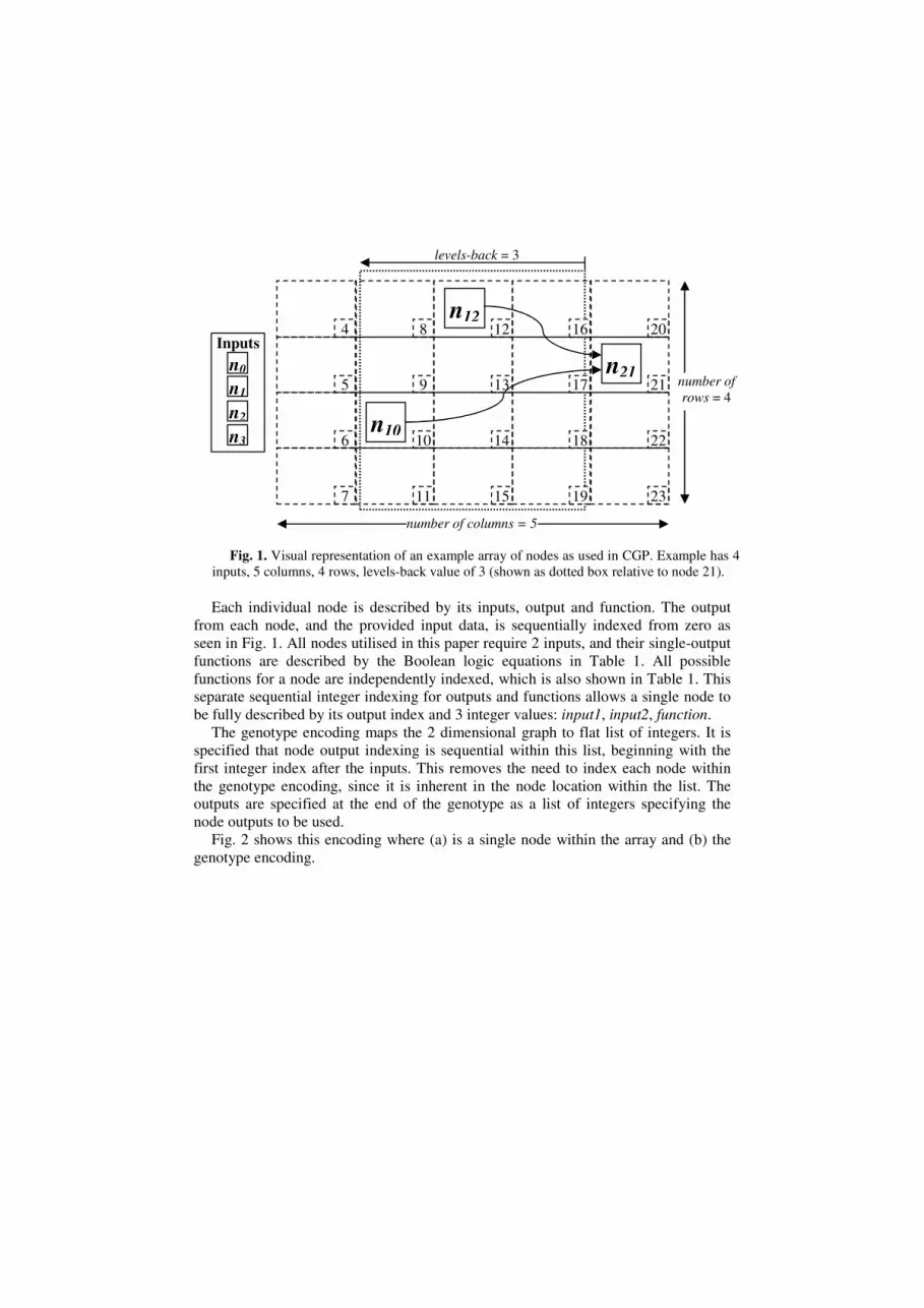
Each individual node is described by its inputs, output and function. The output

from each node, and the provided input data, is sequentially indexed from zero as

seen in Fig. 1. All nodes utilised in this paper require 2 inputs, and their single-output

functions are described by the Boolean logic equations in Table 1. All possible

functions for a node are independently indexed, which is also shown in Table 1. This

separate sequential integer indexing for outputs and functions allows a single node to

be fully described by its output index and 3 integer values: input1, input2, function.

The genotype encoding maps the 2 dimensional graph to flat list of integers. It is

specified that node output indexing is sequential within this list, beginning with the

first integer index after the inputs. This removes the need to index each node within

the genotype encoding, since it is inherent in the node location within the list. The

outputs are specified at the end of the genotype as a list of integers specifying the

node outputs to be used.

Fig. 2 shows this encoding where (a) is a single node within the array and (b) the

genotype encoding.

4 8 12 16 20

5 9 13 17 21

6 10 14 18 22

7 11 15 19 23

n21

n12

n10

levels-back = 3

number of columns = 5

number of

rows = 4

Inputs

n0

n1

n2

n3

Fig. 1. Visual representation of an example array of nodes as used in CGP. Example has 4

inputs, 5 columns, 4 rows, levels-back value of 3 (shown as dotted box relative to node 21).

Table 1. Allowed node functions, as used by Miller [4]

Functional index Logic expression Functional index Logic expression

0 0 10

1 1 11

2 12

3 13

4 14

5 15

6 16

7 17

8 18

9 19

nx

Function Output x

Input 1

Input 2

nx nx+1 Outputs

...... ......

Input 2

Input 1

Function

(a)

(b)

Fig. 2. Graphical representation of how a single node (a) with 2 inputs and a function

index is encoded into the genotype (b).

2.2 Fitness evaluation

To calculate the fitness of a genotype the evolved program’s output is compared

with the desired output as specified in a truth table. To do this comparison, the CGP

program makes efficient use of the processor by carrying out comparisons on multiple

lines of a truth table simultaneously. This technique was introduced by R Poli [6], and

considers a 32-bit processor as 32 individual 1-bit processors for simple logic

functions. Since bit comparison can be achieved by utilising simple logic functions

(See Section 4.1), this technique can be exploited to carry out comparisons of up to 32

lines of a truth table in just a few single-cycle operations. The genotype fitness is then

defined as the total number of correct output bits in the resulting phenotype.

In order for this to be achieved, the desired truth table must be provided in a 32-bit

representation within the configuration file which describes the intended system.

2.3 The Evolutionary Algorithm

A form of the (1 + λ)-ES evolutionary algorithm discussed by Bäck et al [7] is used

throughout this paper. This strategy has also been used by Miller et al [4][5] and been

shown to produce good results. The algorithm implements neutral search whereby if

a parent and offspring have equal fitness, the offspring is always chosen in the

interests of finding neutral solutions. Neutral search has been shown to be crucial to

the efficiency of CGP [1][8]. The algorithm can be described by the following steps:

1. Randomly initialize a population of λ valid genotypes, where constraints

discussed in Section 2.1 are adhered to.

2. Evaluate fitness of each genotype.

3. Identify fittest genotype, giving priority to offspring if parent and offspring

have equal fitness. Copy fittest genotype into the new population to become

the new parent.

4. Produce (λ – 1) offspring to fill population by creating mutated versions of

parent genotype.

5. Destroy old population and return to step 2 using new population, unless a

perfect solution or maximum number generations has been reached.

3 Problem Space

This investigation into the use of “don’t care” logic will be tested by attempting to

evolve the circuits for three problem areas.

3.1 Quotient and Remainder Hardware Divider

Division in microprocessors is most often performed by algorithms such as “shift

and subtract” [9] or SRT (Sweeney, Robertson, and Tocher). Faster algorithms can

also be used such as Newton-Raphson and Goldschmidt, both of which are

implemented in some AMD processors [10]. This paper, however, looks at

developing a simple divider implemented entirely in hardware by standard logic

gates. This circuit is selected as it demonstrates a clearly apparent and understandable

existence of undefined outputs; since calculations involving a division by zero are

mathematically undefined. The divider will take the form of a quotient and remainder

divider, with a single status output for the divide by zero (DIV/0) error.

For 2 inputs A and B, where B is non-zero, this circuit will compute outputs Q and

R to satisfy the following equation:

(1)

For the case where B is equal to zero the solution is undefined and the status output

D goes active (defined as ‘1’ for this case). At this point all of the bits in the both

output buses Q and R are undefined.

As an initial investigation into the performance gains of “don’t care” logic, and in

order to keep the complexity of the tests low, this paper will only consider a 2-bit

divider. The 2-bit divider has 4 single-bit inputs (A1, A0, B1, B0), and 5 single-bit

outputs (Q1, Q0, R1, R0, D). The efficiency of evolution making use of “don’t care”

logic will be compared against using fully-defined logic.

3.2 Finite State Machine Logic

“Don’t care” states often arise when designing next state and output logic for a

finite state machine (FSM). Each state in the FSM must be assigned a binary value,

and hence if the number of states is not an exact power of two there will be unused

binary values. These unused values will result in entire “don’t care” rows in the truth

table.

The FSM used in this paper is of a Mealy structure, where the output(s) depend on

both the current state and current input pattern. The logic to be designed will be

required to produce both the next state value and the output.

The basis for the FSM was chosen to be the MCNC91 benchmark dk27, which has

7 states. The state assignment is therefore 3-bit, and one value is unused (chosen as

000). For simplicity the 2-bit output in the dk27 circuit was flattened into a single bit

output. With the single-bit input this results in a circuit with 4 inputs and 4 outputs,

and two rows of “don’t care” values.

3.3 Distributed Don’t Cares

The previous test cases both result in clusters of “don’t care” values, where all or

most of a row is undefined for specific input patterns. In order to ensure the

experimental results are reflective of a range of circuits, this test case comprises a

truth table designed under the constraints of a maximum of one “don’t care” value per

truth table row.

The circuit was chosen to have 4 inputs and 4 outputs to match the finite state

machine. The outputs were randomly generated, with ones and zeros having equal

probability. The “don’t care” states were also generated randomly, with probability of

a “don’t care” within any row being 50%, and equal probabilities for each output. The

resulting truth table is shown in Table 2.

Table 2. Truth table for the distributed “don't care” circuit, showing maximum of one

undefined output per row.

Inputs Outputs Inputs Outputs

A B C D W X Y Z A B C D W X Y Z

0 0 0 0 1 X 1 1 1 0 0 0 0 1 X 0

0 0 0 1 0 0 1 0 1 0 0 1 X 1 0 1

0 0 1 0 1 1 1 X 1 0 1 0 1 0 1 0

0 0 1 1 1 X 1 1 1 0 1 1 1 1 0 1

0 1 0 0 1 1 0 1 1 1 0 0 0 0 0 1

0 1 0 1 X 0 0 1 1 1 0 1 X 0 1 1

0 1 1 0 X 0 1 0 1 1 1 0 1 0 1 X

0 1 1 1 0 X 1 0 1 1 1 1 1 0 0 0

4 Implementation of Don’t Care Flexibility

4.1 Simple Don’t Care Bitmask

In order to implement “don’t care” logic, it was necessary to add a method of

describing undefined states. In order to maintain efficient fitness evaluation, no

changes were made to the 32-bit truth table representation method. Instead, an

additional section was added describing a 32-bit bitmask for each value in the table.

In this bitmask, a value of ‘1’ indicates the truth table value is valid and fixed, and a

value of ‘0’ indicates flexibility (an undefined value). Before the comparison between

the actual and desired truth table value is carried out, both undergo a logical AND

operation with the bitmask. This process ensures that all undefined states appear as

‘0’ in both the actual and desired truth tables, and hence match. This method allows

for minimal changes to the fitness evaluation code, and thus minimises extra

computational time. The fitness comparison for a single value thus changes from that

in equation (2) to equation (3); where A is the actual output from the phenotype under

evaluation, D is the desired output, and b the bitmask.

. (2)

. (3)

Extra efficiency can be gained if it is ruled that all undefined values are assigned

the value of ‘0’ in the desired truth table, thus the logical AND with the bitmask is not

required for the desired truth table, resulting in equation (4). This comparison requires

only one addition logical operation from the original, and hence should not slow the

fitness evaluation by more than one clock cycle per 32-bit comparison.

. (4)

4.2 Extended Don’t Care Method

The simple “don’t care” method allows evolution the flexibility of exploiting all of

the undefined states. The concept can however be extended further to allow evolution

even more control over exactly how to utilise the undefined outputs.

This is achieved by appending additional genes to the chromosome, to describe

how to interpret each of the available undefined outputs. A simple binary gene

representing whether or not to use each “don’t care” was first considered, however

this method would then restrict evolution to the values encoded in the configuration

file truth table. The extended version instead uses genes with 3 possible values: 0, 1,

or 2. A value of zero or one specifies that the desired output should be interpreted as a

‘0’ or ‘1’ respectively. This effectively removes the “don’t care” from the desired

truth table and replaces it with a zero or one. A value of two represents the desired

output should be considered as a “don’t care” state, and treated as in the simple

method. The fitness evaluation is then the same as for the simple method, however the

desired truth table row and “don’t care” bitmask must be constructed for each

evaluation using the “don’t care” genes in the current chromosome.

5 Evolved Data

5.1 Test Structure and Parameters

The size of the node array was not kept constant for each test case, since the

differing complexities require different array sizes. However the maximum number of

generations was fixed for all tests at 100,000. The gates allowed were 6, 7, 10, 11 and

15 (See Table 1).

For each test circuit the mutation rate was varied, with 100 runs for each mutation

rate executed using: the fully defined truth table, the truth table with “don’t care”

bitmask using the simple strategy, and the truth table with “don’t care” bitmask using

the extended strategy.

5.2 Success of Evolving 2-bit Hardware Divider

The following parameters were used for evolution of the 2-bit hardware divider

detailed in Section 3.1: Number of rows and columns was 4 and levels-back was also.

The mutation rate was varied from 2% to 20% (in steps of 2.0%), and 100 runs for

each mutation rate using each truth table description were executed.

Fig. 3, clearly shows the improved performance of evolution using the flexible

truth table compared with the fully defined truth table. It also highlights the improved

performance of the extended strategy to the simple version for this circuit. Error bars

of plus and minus one standard deviation are plotted in Fig. 3; however all but one are

less than 1.00 and thus may not be visible. This low standard deviation is expected

since it is often only the final 1% of the solution that is the most difficult to evolve, as

shown by [11].

Fig. 3. Graph of the number of perfect solutions reached (out of 100 runs) by using standard

and “don’t care” truth tables for the 2-bit hardware divider.

5.3 Success of Evolving FSM Next State Logic

The FSM next state and output logic is detailed in Section 3.2. The CGP grid was

6x6 with levels back equal to 6. The mutation rate was varied from 2% to 10% (in

steps of 1.0%), and 100 runs for each mutation rate using the fully defined truth table

and each strategy for the incompletely defined truth table were executed.

The results are displayed in Fig. 4, which also shows the improved performance of

evolution using the flexible truth table compared with the fully defined truth table. In

contrast to the hardware divider, the simple “don’t care” strategy outperforms the

extended version for this circuit. Error bars of plus and minus one standard deviation

are plotted.

5.4 Success of Evolving Distributed Don’t Cares Circuit

Since this circuit was designed to mimic the complexity of the FSM logic, the same

experimental parameters were used. The mutation rate was also varied from 2% to

10% in steps of 1.0%. The results are displayed in Fig. 5, which once again supports

previous results of improved performance using the flexible truth table compared with

the fully defined truth table. The simple “don’t care” strategy also outperforms the

extended version for this circuit. Error bars of plus and minus one standard deviation

are plotted in Fig. 5.

Fig. 4. Graph of the number of perfect solutions reached (out of 100 runs) by using standard

and “don’t care” truth tables for the FSM next state and output logic.

5.5 Efficiency of Evolved Circuits

Whilst it is advantageous to consider the computational benefits of the flexible truth

table, perhaps more exciting is to consider the hardware efficiency of the evolved

solutions. To enable evolution to continue beyond the initial perfect solution and

attempt to reduce hardware requirements, the genotype fitness for perfect circuits

must be modified. The simple modification defines fitness for perfect genotypes as

the maximum fitness plus the number of redundant nodes (nodes which do not

contribute to the outputs). This causes the algorithm to always run until the maximum

number of generations is reached, attempting to reduce the number of active nodes.

This algorithm was executed on each test case with the parameters and varying

mutation rates given in previous sections. The array size was also varied, up to a

maximum of 100 available nodes.

Conventional methods such as the Karnaugh map allow minimised Boolean

equations to be obtained from a desired truth table (See [12] for a good explanation).

The Karnaugh map can be used to identify a benchmark for the hardware

requirements of the test circuits. A Karnaugh map was constructed for each of the

outputs of each circuit, and the sum-of-products Boolean equations obtained.

Restricting the logic gates to only those available to the evolved circuits, the number

of 2-input gates required to synthesise each circuit can be found. This is shown in

Table 3.

Table 3. Number of 2-input gates required to synthesis test circuits from Karnaugh map

minimised sum-of-products

Circuit Number of 2-input gates required

2-bit Divider 16

FSM Logic 41

Distributed Don’t Cares 35

Fig. 5. Graph of the number of perfect solutions reached (out of 100 runs) by using standard

and “don’t care” truth tables for the distributed “don’t care” circuit.

Hardware divider: The most efficient solution in terms of hardware requirements for

the hardware divider was found to require 8 gates, a hardware saving of 50%

compared with that found by conventional methods in Table 3. This solution used the

simple “don’t care” strategy. It is worth noting that without the “don’t care”

modification, the most efficient solution required 10 gates.

Finite State Machine Logic: The most hardware efficient design for the finite state

machine next state and output logic required 14 gates, a hardware saving of 66%. This

solution was also found using the simple “don’t care” strategy, and the most efficient

solution without truth table flexibility required 19 gates.

Distributed Don’t Cares: Once again the simple strategy outperformed the extended

version for finding efficient solutions, with the least number of gates required being

15. Without any truth table flexibility, a solution requiring 18 gates was also

achieved.

Clearly, the extended strategy for “don’t care” utilisation does not offer any

benefits to the simple version for finding efficient circuits. The use of flexible truth

tables does however have a clear advantage, resulting in at least a 20% reduction in

hardware for all three test circuits, compared with standard CGP.

6 Conclusion

The motivation behind introducing flexibility in the desired truth table has been

discussed in this paper, and a method for implementing this technique using a “don’t

care” bitmask has been shown. Two strategies have been introduced for making use

of available undefined states, and it has been shown that the best strategy is dependent

on the circuit under test. Using three circuits with incompletely defined truth tables,

the use of unfixed output values has been demonstrated to increase the performance of

CGP, as well as producing more hardware efficient designs.

Allowing “don’t care” logic in the truth table can be thought of as increasing the

potential number of perfect truth tables, and hence perfect phenotypes. Since CGP

already has a many-to-one genotype-phenotype mapping, increasing the number of

perfect phenotypes significantly increases the number of perfect fitness genotypes.

This greatly increases the level of neutrality in the search space, which has been

shown to improve performance [1][8]. Considered from this perspective, the results

found in this paper agree with those found by Miller et al.

7 Bibliography

1. Miller, J. F., Thomson P. Cartesian Genetic Programming. Proc. European Conf.

on Genetic Programming. Springer LNCS 1802 (2000) 121-132.

2. Miller, J. F, Evolution of Digital Filters using a Gate Array Model, Proceedings

of the EvoIASP'99 Workshop on Image Analysis and Signal Processing, Springer

LNCS Vol. 1596 (1999) pp. 17-30.

3. Miller, J. F, Digital Filter Design at Gate-level using Evolutionary Algorithms,

Proc. Genetic and Evolutionary Computation Conference (1999) pp. 1127-1134.

4. Miller, J. F, Job D., Vassilev V.K. Principles in the Evolutionary Design of

Digital Circuits - Part I. Journal of Genetic Programming and Evolvable

Machines, 1 (2000) 8-35.

5. Miller, J. F., Thomson, P., and Fogarty, T., Designing Electronic Circuits Using

Evolutionary Algorithms. Arithmetic Circuits: A Case Study, Genetic Algorithms

and Evolution Strategies in Engineering and Computer Science, D. Quagliarella,

J. Periaux, C. Poloni, and G. Winter (eds.), Wiley (1997) pp. 105-131.

6. Poli, R., Sub-machine-code GP: New results and extensions, in Proceedings of

the 2nd European Workshop on Genetic Programming, R. Poli, P. Nordin, W. B.

Langdon, and T. Fogarty (eds.), Springer, LNCS Vol. 1598 (1999) pp. 65-82.

7. Bäck, T., Hoffmeister, F., Schwefel, H. P., A survey of evolution strategies, in

Proceedings of the 4th International Conference on Genetic Algorithms, R.

Belew and L. Booker (eds.), Morgan Kaufmann (1991) pp. 2-9

8. Miller J.F., Smith S.L. Redundancy and Computational Efficiency in Cartesian

Genetic Programming. IEEE Trans. on Evol. Comput., 10 (2006) pp. 167-174

9. R.F. Shaw. Arithmetic Operations in a Binary Computer. The Review of

Scientific Instruments Volume 21, Number 8, 1950.

10. Stuart F. Oberman, "Floating Point Division and Square Root Algorithms and

Implementation in the AMD-K7 Microprocessor", in Proc. IEEE Symposium on

Computer Arithmetic, pp. 106-115, 1999

11. J. R. Koza, Genetic Programming: On the Programming of Computers by Means

of Natural Selection, MIT Press: Cambridge, MA, 1992.

12. Holder, M.E., "A modified Karnaugh map technique," Education, IEEE

Transactions on , vol. 48, no.1, pp. 206-207, Feb. 2005