A KdV-like advection–dispersion equation with some remarkable properties

This article appeared in a journal published by Elsevier. The attachedcopy is furnished to the author for internal non-commercial researchand education use, including for instruction at the authors institution

and sharing with colleagues.

Other uses, including reproduction and distribution, or selling orlicensing copies, or posting to personal, institutional or third party

websites are prohibited.

In most cases authors are permitted to post their version of thearticle (e.g. in Word or Tex form) to their personal website orinstitutional repository. Authors requiring further information

regarding Elsevier’s archiving and manuscript policies areencouraged to visit:

http://www.elsevier.com/copyright

http://www.elsevier.com/copyright

Author's personal copy

A KdV-like advection–dispersion equation with someremarkable properties

Abhijit Sen a,⇑, Dilip P. Ahalpara a, Anantanarayanan Thyagaraja b, Govind S. Krishnaswami c

a Institute for Plasma Research, Bhat, Gandhinagar 382 428, Indiab H.H. Wills Physics Laboratory, University of Bristol, Tyndall Avenue, BS8 1TL, UKc Chennai Mathematical Institute, SIPCOT IT Park, Siruseri 603103, India

a r t i c l e i n f o

Article history:Received 4 February 2012Received in revised form 26 February 2012Accepted 1 March 2012Available online 9 March 2012

Keywords:Genetic programmingAdvection dispersion equationTravelling wavesRecurrence

a b s t r a c t

We discuss a new non-linear PDE, ut þ ð2uxx=uÞux ¼ �uxxx , invariant under scaling of depen-dent variable and referred to here as SIdV. It is one of the simplest such translation andspace–time reflection-symmetric first order advection–dispersion equations. This PDE(with dispersion coefficient unity) was discovered in a genetic programming search forequations sharing the KdV solitary wave solution. It provides a bridge between non-linearadvection, diffusion and dispersion. Special cases include the mKdV and linear dispersiveequations. We identify two conservation laws, though initial investigations indicate thatSIdV does not follow from a polynomial Lagrangian of the KdV sort. Nevertheless, it pos-sesses solitary and periodic travelling waves. Moreover, numerical simulations revealrecurrence properties usually associated with integrable systems. KdV and SIdV are thesimplest in an infinite dimensional family of equations sharing the KdV solitary wave. SIdVand its generalizations may serve as a testing ground for numerical and analytical tech-niques and be a rich source for further explorations.

� 2012 Elsevier B.V. All rights reserved.

1. Introduction

Several equations of physics have been discovered by searching for one that admits a particular type of solution that wasknown to exist on physical grounds. Perhaps the most celebrated example is the discovery of Schrödinger’s equation of quan-tum mechanics via de Broglie’s hypothesis that free particles are described by plane matter waves. The KdV equation of fluidflow in a canal [1],

ut þ 6uux þ uxxx ¼ 0 ð1Þ

was motivated (and in part discovered) by the search for an equation possessing Scott Russell’s [2] ‘wave of translation’ as asolution. This is the solitary wave

uðx; tÞ ¼ c2

sech2ffiffifficp

2ðx� ct � x0Þ

� �for c > 0; x0 2 R: ð2Þ

The KdV equation is the simplest conservative 1-dimensional wave equation with weak advective non-linearity and disper-sion. Thus it is widely applicable and has been used to model acoustic solitons in plasmas [3,4], internal gravity waves [5] inthe oceans and even blood pressure pulses [6]. Its significance was greatly amplified by Zabusky and Kruskal’s discovery [3]

1007-5704/$ - see front matter � 2012 Elsevier B.V. All rights reserved.http://dx.doi.org/10.1016/j.cnsns.2012.03.001

⇑ Corresponding author. Tel.: +91 9825051578; fax: +91 7923969016.E-mail address: [email protected] (A. Sen).

Commun Nonlinear Sci Numer Simulat 17 (2012) 4115–4124

Contents lists available at SciVerse ScienceDirect

Commun Nonlinear Sci Numer Simulat

journal homepage: www.elsevier .com/locate /cnsns


that KdV displays the Fermi–Pasta–Ulam recurrent behavior and lack of thermalization [7] in a spatially periodic domain(see also [8,9]). This was subsequently attributed to the even more remarkable asymptotic superposition principle for scat-tering of KdV solitary waves and existence of infinitely many local conserved quantities in involution [10]. Moreover, KdV isthe prototype for an integrable non-linear PDE, its initial value problem can be solved by the inverse scattering transform[11].

We were therefore excited to find that the KdV equation is not the only one with the sech2 solitary wave solution. Thisserendipitous discovery happened in the course of an investigation undertaken by two of the present authors [12] to improvethe efficiency and accuracy of a genetic programming (GP) based method (see Appendix A) to deduce model equations from aknown analytic solution [13]. As a benchmark exercise to test out the method for application to nonlinear PDEs, the travel-ling wave (2) was given to the program, expecting it to find the KdV equation. But, surprisingly, before finding the KdV equa-tion, it found a different equation

ut þ2uxx

u

� �ux ¼ uxxx; ð3Þ

which had the same solitary wave solution. Subsequently, we found that (3) is the simplest in a vast family of equations shar-ing the KdV solitary wave. We think of (3) as a non-linear wave equation for the dispersive advection of the real wave ampli-tude u. Unlike the KdV equation, where the advecting velocity V ¼ 6u is linear, here it is a quotient V ¼ ð2uxx=uÞ. As aconsequence (3) is ‘scale-invariant’ under dilation u! ku of dependent variable. Scale-invariant advective velocities have ap-peared before e.g., the E�B

B2 velocity that is invariant under a rescaling of fields, charges and currents in a plasma. We refer to(3) as the (� = 1 case of the) SIdV equation.1 Like KdV, faster SIdV solitary waves are narrower, but due to scale invariance,height and speed are generally unrelated, as in classical linear wave equations, but unlike KdV and the non-linear Schrödingerequation (NLSE).

In (3) the dimension-L3=T coefficients of the dispersive and advective terms are both equal to one. This is of course veryspecial. More generally we consider the SIdV equation

ut þ2auxx

u

� �ux ¼ �auxxx: ð4Þ

x!ffiffiffia3p

x eliminates the L3=T-dimensional constant a, leaving one dimensionless parameter � measuring the strength of dis-persion relative to advection. Unlike KdV, where they scale differently in x, here both scale as L�3. Though we have not foundan experimental system modelled by (4), it is just as simple and universal among scale-invariant advection–dispersion equa-tions as KdV is among all such equations. For generic �, we have identified 2 conserved densities. This is similar to inviscidEulerian hydrodynamics, but unlike KdV and NLSE which possess an infinite number. While SIdV shares solitary waves withKdV at � = 1, non-linear diffusion and solvability emerge elsewhere. Despite being non-linear, scale-invariance ensures SIdVhas exact plane wave solutions. Furthermore, it possesses bounded spatially periodic travelling waves and similarity solu-tions. However, SIdV cannot arise from a polynomial Lagrangian in the sort of variable that works for KdV. We evade thisobstruction at some special values of �. Remarkably, numerical evolution of (3) shows Fermi–Pasta–Ulam-like Birkhoff recur-rence [9] despite no sign of soliton scattering!

2. General properties of the SIdV equation

2.1. Symmetries and conservation laws

SIdV (4) is a non-linear advection–dispersion equation for the real wave amplitude u(x, t) that is being advected by theflow V ¼ 2uxx=u. It is scale-invariant2 under u! ku. In fact, (4) is the simplest non-linear translation and scale-invariant advec-tion–dispersion equation that is first order in time. The lowest order dispersive term is uxxx, so any such equation can be writtenas ut þ Vux ¼ a�uxxx for some scale-invariant advective velocity V. Without requiring scale-invariance, the simplest choice V / uleads to KdV. KdV is symmetric under space–time (PT) reflection ðx; tÞ ! ð�x;�tÞ. Now if we also require scale-invariance, thesimplest advecting velocities that preserve PT symmetry are V / uxx

u and uuxx

. The former leads to (4) in units where a ¼ 1. Thelatter choice too has some notable properties (see Section 7).

Non-zero constants are the simplest solutions of (4). Linearization about a constant yields a plane wave with cubic dis-persion x ¼ �k3 and the characteristic property that the ratio of phase to group velocity is 1/3, as in the linear KdV equation.Remarkably, despite being non-linear, (4) also admits exact plane wave solutions u ¼ A sin kx� ð�� 2Þk3t þu

� �.

KdV is invariant under Galilean boosts x! xþ ct if u transforms as u! uðxþ ct; tÞ � ðc=6Þ. However, SIdV is not invariantunder du ¼ bþ ctux for any constants b and c – 0. However, Galilean boosts could be implemented in a more intricate man-ner that we have not identified.

Multiplying by u, and using uu3x ¼ uuxx � 12 u2

x

� �x, (4) is written in conservation form

1 The acronym SIdV highlighting scale-invariance is related to KdV as Sine–Gordon is related to Klein–Gordon.2 SIdV (4) is not invariant under dilations of x and has a dimensional scale a which we set to 1.

4116 A. Sen et al. / Commun Nonlinear Sci Numer Simulat 17 (2012) 4115–4124


12½u2�t þ 1þ �

2

� �u2

x � �uuxx

x¼ 0: ð5Þ

It follows that I ¼R

u2dx is conserved. This suggests u2 is the concentration of some substance whose total amount is con-served. Similarly, multiplying (4) by u�2=� we get

u1�2=�� t þ ð2� �Þ u�2=�uxx

� �x ¼ 0: ð6Þ

So J ¼R

u1�2=�dx is also conserved. For e.g., when � ¼ 1; J ¼R

1u dx, so on a bounded domain, J is finite for any strictly positive/

negative initial condition. These integrals of motion, travelling waves (Section 3.2) and numerical evolution (Section 5) indi-cate that SIdV is generically non-dissipative.

2.2. Preservation of positivity of u(x)

At first sight, it appears that u = 0 is a singular point of (4). But u can vanish at points where ux or uxx also vanish, provideduxxux=u is finite, e.g., the above plane wave vanishes at isolated points. Among travelling waves, this is generic, near onewhere u and uxx have common zeros, there is another solution with the same property. However, in the numerical and ana-lytical examples studied, if uðx;0Þ > 0, it remains positive for t > 0. Let us use the second conserved quantity J ¼

R1u dx to

sketch why this is the case for � = 1 on a bounded domain.3 Suppose uðx;0Þ > 0 and J is finite at t ¼ 0. At t1 > 0, let uðxÞ developits first zero, this cannot be a first-order zero as u was strictly positive. Then Jðt1Þ ¼ 1, contradicting the constancy of J! Sostrictly positive initial data cannot develop a zero and therefore must remain positive4.

2.3. Behaviour of SIdV at some special values of dispersion coefficient

2.3.1. Reduction to a linear dispersive wave equation when � ¼ �2=3For � ¼ �2=3, SIdV may be reduced to a linear dispersive equation for u2. If we write uuxx ¼ ðuuxÞx � u2

x ¼ 12 ðu2Þx � u2

x in theconservation law form (5) of SIdV, we get

12@tu2 þ @x 1þ 3�

2

� �u2

x ��2

u2� �xx

¼ 0: ð7Þ

If � ¼ �2=3, we see that q ¼ u2 satisfies a linear KdV equation

qt þ23qxxx ¼ 0: ð8Þ

So for � ¼ � 23 ;q ¼ u2 is a sort of Cole–Hopf transformation that linearizes the equation. The general solution is a linear com-

bination of plane waves

qðx; tÞ ¼ u2ðx; tÞ ¼Z

R

~qðkÞei kxþ23k3tð Þ dk

2pwhere ~qðkÞ ¼

ZR

u2ðx;0Þe�ikxdx: ð9Þ

This solution could serve as the 0th order of a perturbative solution of SIdV for nearby �.

2.3.2. The dispersionless limit � = 0The special case � = 0 of (4) gives a non-dispersive non-linear advection equation

ut þ2uxx

uux ¼ 0: ð10Þ

It may be written as a conservation law ðu2Þt þ ð2u2x Þx ¼ 0 for the ‘charge’ density u2 with flux u2

x . Being a second orderparabolic PDE, (10) may also be viewed as an unusual non-linear diffusion equation ut ¼ auxx for the ‘temperature’ u. Theeffective thermal diffusivity a ¼ �2ux=u could be of either sign. Thus SIdV is a remarkable bridge connecting dispersion,non-linear advection and non-linear diffusion. We expect (10) to have instabilities if a becomes negative since time-reversedheat equations are ill-posed. So we may think of the dispersive term in SIdV as a regularization of (10), just as KdV is aregularization of the kinematic wave equation (KWE) ut þ 6uux ¼ 0. Remarkably, even without a dispersive regularization,(10) has smooth solutions. Indeed, unlike the KWE, (10) admits waves that preserve their shape. The general travelling waveof (10) is u ¼ A cosðkxþ 2k3t þ /Þ. These plane waves may however be unstable, as the diffusivity oscillates in sign!

3 A similar argument can be given for any e for which a conserved density diverges at u ¼ 0 sufficiently fast.4 We assume that uðxÞ cannot develop an ‘integrable’ zero for which J is finite. An ‘integrable’ zero where u � jxja for a < 1 would mean u forms a cusp and

ceases to be thrice continuously differentiable. Assuming the solution remains sufficiently smooth, such possibilities are eliminated. Our numerical simulationsdid not indicate cusp formation, though it is an open question whether SIdV preserves regularity of initial data.

A. Sen et al. / Commun Nonlinear Sci Numer Simulat 17 (2012) 4115–4124 4117


2.3.3. SIdV to mKdV when � ¼ 2=3We did not find any value of � at which a transformation reduces the SIdV to the KdV equation. But there are special val-

ues of � at which it comes close. First, the rational non-linearity of SIdV can be written as a polynomial while retaining theadvection–dispersion structure of the equation. To do so, we use the invariance of SIdV under rescaling to choose u dimen-sionless and put u ¼ ew. Then5

wt þ ð2� �Þw2x þ ð2� 3�Þwxx

� �wx ¼ �wxxx: ð11Þ

This polynomial form of SIdV was convenient for numerical evolution and also in our search for a Lagrangian. It also indicatesthat � ¼ 2; 2

3 are somewhat special. At these values, we get KdV-like dispersive wave equations with advecting velocities/ w2x

and wxx. These are among the simplest PT symmetric advecting velocities beyond KdV. Moreover, at � = 2/3, the sign of the‘local diffusivity’ is reversed. We see qualitative effects of this reversal in the stability of our numerical simulations as � isdecreased below 2/3. What is more, at � = 2/3 SIdV is reducible to the modified KdV (mKdV) equation. Differentiating in xat � = 2/3, putting v = wx and letting x! �x and t ! 3

2 t, we get the defocusing mKdV equation, which is integrable and re-lated to KdV via the Miura transform [14]

v t � 6v2vx þ v3x ¼ 0: ð12Þ

3. Some similarity and travelling wave solutions of SIdV

3.1. Similarity solutions

SIdV is invariant under6 x! kx and t ! k3t. So we seek solutions uðx; tÞ ¼ f ðzÞ in the similarity variable z ¼ x3=54t. We get athird order non-linear ODE for f(z)

�z2

2f 000f � z2f 00f 0 þ �zf 00f � 2z

3f 02 þ �

9þ z

� �f 0f ¼ 0: ð13Þ

By the substitution g ¼ f 0=f we reduce this to a cubic 2nd order ODE with variable coefficients

�z2

2g00 þ 3�

2� 1

� �z2gg0 þ �zg0 þ �

2� 1

� �z2g3 þ �� 2

3

� �zg2 þ �

9þ z

� �g ¼ 0: ð14Þ

We have not solved the similarity ODE in general, but in the dispersionless limit � = 0, it becomes a linear ODE with a regularsingularity at z = 0

zf 0 þ 23

f 0 � f ¼ 0: ð15Þ

The two linearly independent solutions may be expressed in terms of the confluent hypergeometric function 0F1(a,z) or themodified Bessel function of the 1st kind In(z):

f1ðzÞ¼0F123; z

� �¼ 1þ 3z

2þ . . . ¼ C

23

� �z

16I�1

32ffiffiffizp� �

and

f2ðzÞ ¼ z130F1

43; z

� �¼ z

13 1þ 3z

4þ . . .

� �¼ C

43

� �z

16I1

32ffiffiffizp� �

: ð16Þ

Both f1 and f2 are monotonic and grow / e2ffiffizp

as z!1. So they are bounded at late times (z! 0 or t � x3) but are un-bounded at early times (z!1 or x3 � t ! 0). Interestingly, there is a unique (up to scale) linear combinationf ðzÞ ¼ Cð4=3Þf1ðzÞ � Cð2=3Þf2ðzÞ that is bounded for all z P 0 ðx; t P 0Þ. It begins at f ð0Þ ¼ Cð4=3Þ and monotonically decaysto zero as z!1.

3.2. Travelling waves

Here we discuss travelling waves (u ¼ f ðnÞwith n ¼ x� ct) for SIdV (4) on the unbounded domain�1 < n <1. Travellingwaves must satisfy the third order non-linear ODE �cff 0 þ 2f 0f 0 � �ff 000 ¼ 0. We may write this in ‘conservation law’ form

� c2ðf 2Þ0 þ 2þ �

2ðf 02Þ0 � �ðff 00Þ0 ¼ 0 ð17Þ

5 Of course, if we restrict to real w, this equation will apply to solutions where u remains everywhere positive.6 More generally, SIdV is invariant under x! kx; t ! k3t;u! kcu for any c. So t�c=3uðx; tÞ ¼ f ðzÞ is a scale invariant combination. Since c is arbitrary, we

restrict here to the simplest case c ¼ 0.



and integrate once to get

2�ff 00 � ð�þ 2Þf 02 þ cf 2 þ 3B ¼ 0: ð18Þ

The substitutions p ¼ f 0 and F ¼ p2 give us a first order linear ODE for Fðf Þ:

�fF 0ðf Þ � ð�þ 2ÞF þ cf 2 þ 3B ¼ 0 or �F 0ðwÞ � ð�þ 2ÞF þ ce2w þ 3B ¼ 0; ð19Þ

where f ¼ ew. This inhomogeneous 1st order ODE is reduced to quadrature using the integrating factor e�ð1þ2=�Þw. For �– 0, interms of rðwÞ ¼ e�ð1þ2=�ÞwFðwÞ, we get

�r0 þ 3Be�ð1þ2=�Þw þ ceð1�2=�Þw ¼ 0: ð20Þ

For �– 0;�2, we integrate to get

FðwÞ ¼ Aeð1þ2�Þw þ c�e2w

2� � þ3B�þ 2

: ð21Þ

In other words, the equation for travelling waves has been reduced to quadrature

Zdn ¼ �

ZdfffiffiffiffiffiffiffiffiffiFðf Þ

p where F ¼

c2 f 2 þ 3B

2 if � ¼ 0:12 Af 2 � cf 2 log f þ 3B

4 if � ¼ 2;c4 f 2 þ 3B

2 log f � 12 A if � ¼ �2; and

Af ð1þ2�Þ þ c�

2��

f 2 þ 3B�þ2 otherwise:

8>>>>><>>>>>:

ð22Þ

This travelling wave integral can be understood by a mechanical analogy [14]. It is the zero ‘energy’ conditionE ¼ f 02 þ Vðf Þ ¼ 0 for the ‘coordinate’ f ðnÞ at ‘time’ n of a non-relativistic particle of mass 2 moving in the 1-dimensional po-tential Vðf Þ ¼ �Fðf Þ. Bounded travelling waves correspond to bound trajectories of this particle. Plotting V(f) shows that, forappropriate ranges of A, B and c, there are bounded spatially periodic/solitary travelling waves with heights between succes-sive real simple/double zeros of V(f). For generic �, the travelling wave integral

RF�1=2df cannot be evaluated using elemen-

tary functions. But for � ¼ 1;0;�2=3, the integral is trigonometric/exponential and for � ¼ 2=3;1 it is elliptic.To illustrate, we consider the case � = 1 where SIdV shares solitary wave solutions with KdV. Here we must evaluate an

elliptic integralRðAf 3 þ cf 2 þ BÞ�1=2df , and bounded travelling waves are (limits of) cnoidal waves. Suppose A > 0 and

Fðf Þ ¼ Af 3 þ cf 2 þ B ¼ Aðf � f1Þðf � f2Þðf � f3Þ has three simple real zeros 0 P f1 < f2 < f3 P 0. Then we have a periodic cnoi-dal wave with trough at f1 and crest at f2, determined by

�ðn� n1Þ ¼Z f

f1

dgffiffiffiffiffiffiffiffiffiffiffiffiffiffiffiffiffiffiffiffiffiffiffiffiffiffiffiffiffiffiffiffiffiffiffiffiffiffiffiffiffiffiffiffiffiffiffiffiffiffiffiAðg � f1Þðg � f2Þðg � f3Þ

p where f ðn1Þ ¼ f1: ð23Þ

Transforming to g ¼ f1 þ ðf2 � f1Þ sin2 h and defining the shape parameter 0 6 m ¼ f2�f1f3�f16 1, (23) becomes a standard incom-

plete elliptic integral of the first kind. It is inverted in terms of a Jacobi elliptic function cnðu; mÞ ¼ cos /, with moduluskðm ¼ k2Þ

n ¼ n1 �2uffiffiffiffiffiffiffiffiffiffiffiffiffiffiffiffiffiffiffiffi

Aðf3 � f1Þp where u ¼

Z /

0

dhffiffiffiffiffiffiffiffiffiffiffiffiffiffiffiffiffiffiffiffiffiffiffiffiffiffi1�m sin2 h

p : ð24Þ

At the upper limit g ¼ f ¼ f2 � ðf2 � f1Þ cos2 /, so the cnoidal wave for A > 0 is

f ¼ f2 � ðf2 � f1Þcn2 12

ffiffiffiffiffiffiffiffiffiffiffiffiffiffiffiffiffiffiffiffiAðf3 � f1Þ

qðn� n1Þ; m

� �: ð25Þ

Its shape depends on m while its wavelength and speed are

k ¼ 4KðmÞffiffiffiffiffiffiffiffiffiffiffiffiffiffiffiffiffiffiffiffiAðf3 � f1Þ

p and c ¼ �Aðf1 þ f2 þ f3Þ: ð26Þ

Here KðmÞ ¼R p=2

0dhffiffiffiffiffiffiffiffiffiffiffiffiffiffiffiffi

1�m sin2 hp is the complete elliptic integral of the 1st kind.

The advecting velocity field V ¼ 2f 00

f for cnoidal waves is finite since f and f 00 have common zeros. Moreover, by modifyingthe parameters A; fi, we get nearby waves with the same feature. Unlike for KdV, where the shape, speed and wavelength ofcnoidal waves are non-trivially modified upon a rescaling of amplitude, here f # kf produces a new cnoidal wave with thesame m; c; k and phase n1, since the constants transform as ðA;B; fiÞ# ðA=k; k2B; kfiÞ.

If A < 0, the cnoidal wave extends between f2 and f3 and is given by

f ðnÞ ¼ f2 þ ðf3 � f2Þcn2 12


qðn� n3Þ; ~m

� �; ð27Þ

where ~m ¼ ðf3 � f2Þ=ðf3 � f1Þ and k ¼ 4Kð ~mÞffiffiffiffiffiffiffiffiffiffiffiffiffiffiffiffiffiffiffiffiAðf1 � f3Þ

p.



Solitary waves are cnoidal waves of infinite wavelength. They occur when a pair of simple zeros of F coalesce to form adouble zero. For example, if f3 ! f2 in (25) holding f1;2 and A > 0 fixed, then m! 1�;KðmÞ ! 1 and we get a left-moving sol-itary wave of depression

f ðnÞ ! f2 � ðf2 � f1Þsech2 12


qðn� n1Þ

� �for A > 0: ð28Þ

If the zeros f1 ! f2 coalesce in (27) we get a left-moving solitary wave of elevation

f ðnÞ ! f2 þ ðf3 � f2Þsech2 12


qðn� n3Þ

� �for A < 0: ð29Þ

Finally, if A! 0, cnoidal waves reduce to sinusoidal waves with cubic dispersion,

f ðnÞ ¼ N sinffiffiffiffiffiffi�cp

n� n0ð Þ� �

; c < 0;N arbitrary: ð30Þ

4. Search for a variational principle for SIdV

To relate symmetries to integrals of motion, it is interesting to find a Lagrangian or Hamiltonian formulation for SIdV. Theexistence of a Lagrangian for a given equation depends on the field variables used and the sort of Lagrangian allowed. Forinstance, the dispersive term uxxx in KdV ut þ 6uux þ uxxx ¼ 0 is not the variation of any polynomial in u and its derivatives.This is because every quadratic differential polynomial in u involving three x-derivatives is a total derivative. Yet, as is well-known, if we put u ¼ vx, KdV follows from the Lagrangian density 1

2 vtvx � v3x � 1

2 v2xx.

In looking for a Lagrangian for SIdV, we choose to work with w ¼ log u, which satisfies the KdV-like Eq. (11) with poly-nomial non-linearity. By analogy with KdV, we put w ¼ /x and seek a polynomial action in / and its derivatives, whose Euler–Lagrange (EL) equations are

/xt þ ð2� �Þ/2xx þ ð2� 3�Þ/xxx

� �/xx ¼ �/xxxx: ð31Þ

/ is a natural variable since the linear part of the equation /xt ¼ �/4x admits the polynomial Lagrangian L0 ¼ 12 /t/x þ �

2 /2xx.

We wish to add potentials V ;W to L0 to reproduce the quadratic /xx/3x and cubic terms /3xx in (31). To do so, we note a couple

of general features. If V is a monomial of degree n in / and its x-derivatives, then (1) the resulting terms in the EL equationform a differential polynomial of degree n� 1, and (2) the total number of x-derivatives in each term of the differential poly-nomial are the same as in V. Therefore, to produce /3

xx in the EL equation, W must be a quartic differential polynomial with 6x-derivatives, and to give /xx/3x;V must be a cubic differential polynomial with 5 derivatives. In other words,

V ¼ a1///5x þ a2//x/4x þ a3//2x/3x þ a4/x/x/3x þ a5/x/2x/2x ¼X

i

aiV i: ð32Þ

Can ai be chosen so that the variation ofR

Vdx gives ð2� 3�Þ/xx/3x? Unfortunately not, as7

dd/ðxÞ

ZVð/ðyÞÞdy ¼ �ð10a1 � 5a2 þ a3 þ 4a4 � 2a5Þð2/xx/xxx þ /x/4xÞ: ð33Þ

For no choice of ai can we produce just a quadratic monomial / /xx/xxx in the EL equation. Similarly, we showed that there isno quartic differential polynomial W that gives /3

xx upon variation. We conclude that there is no polynomial Lagrangian in /and its derivatives leading to SIdV.

However, the polynomiality assumption is quite strong. There may be a non-polynomial Lagrangian in / or one in a var-iable non-locally related to /. An interesting example of such a possibility occurs when � ¼ � 2

3 and SIdV becomes the lineardispersive equation qt þ ð2=3Þqxxx ¼ 0 upon substituting q ¼ u2. This equation follows from L ¼ 1

2 wtwx � 13 w2

xx, where wx ¼ q.However, w ¼

R xe2/y dy is non-locally related to /, so the Lagrangian is non-local in /.Another way around this negative result is that there may be a Hamiltonian that is a differential polynomial in /, but with

non-canonical Poisson brackets. Such a possibility is realized if � ¼ 2=3, when SIdV can be transformed into the mKdV equa-tion v t � 6v2vx þ v3x ¼ 0 by the substitution v ¼ ux

u and a rescaling (Section 2.3.3). mKdV admits a Hamiltonian formulationv t ¼ fH;vg with

H ¼ 12

Zv2

x þv4

6

� �dx and fvðxÞ;vðyÞg ¼ �@xdðx� yÞ: ð34Þ

So for � ¼ 2=3, SIdV admits a polynomial Hamiltonian in the variable v ¼ ðlog uÞx ¼ wx ¼ /xx. It would be interesting to find aHamiltonian/Lagrangian formulation of SIdV for other values of �.

7 In particular, this means all the Vi differ from one another by total x-derivatives.



5. Numerical evolution of SIdV solitary waves: recurrent behavior

We numerically solved8 the SIdV initial value problem for � = 1 on the interval ½�p;p� with periodic boundary conditions.Numerical evolution of one sech2 wave produced a right-moving travelling wave, as expected from the exact solution onð�1;1Þ. We also considered two solitary waves9

uðx;0Þ ¼X

j

A1sech2ffiffiffiffiffic1p

2ðx� x1 þ 2pjÞ

� �þ A2sech2

ffiffiffiffiffic2p

2ðx� x2 þ 2pjÞ

� �: ð35Þ

When the two solitary waves were initially separated by some distance but had the same heights and speed, they were ob-served to travel without much interaction, just like individual solitary waves.

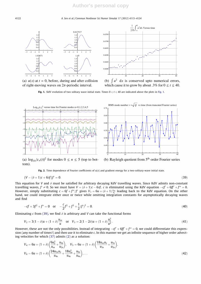
Next, we gave the two waves the same initial amplitudes A1;2 ¼ 1 but different speeds (or widths) ðc1; c2Þ ¼ ð4;2Þ andlocations ðx1; x2Þ ¼ ð�p=2;p=4Þ at t ¼ 0 (Fig. 1(a)). So it would take each wave by itself a time of p

2 and p to traverse the2p-interval. Solitary waves that decay at 1 must be right-moving, so we couldn’t give them opposing velocities. Butc1 > c2, so wave-1 caught up with wave-2 due to periodic boundary conditions and collided with it from the rear. Then theyseparated into a small leading wave and a larger trailing wave. The original solitary waves did not retain their shapes. Thesmaller wave that emerged from the collision moved faster and caught up with the bigger one by going round the circle.During the next collision, the smaller wave rear-ended the larger one. The large one in front morphed into a fast small wave,leaving behind a slow large wave. This is illustrated in the last three plots of Fig. 1(a). Qualitatively, this pattern seemed torepeat as the IVP was solved up to t = 40, allowing more than two dozen collisions to be observed.10

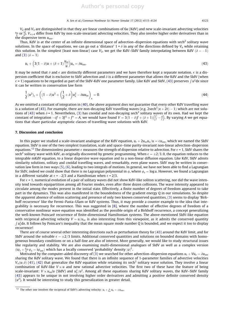
Though not KdV solitons, the solitary waves that were involved in these collisions displayed a certain coherence, they didnot dissipate nor degenerate into ripples. Despite not being periodic, the evolution seemed to approximately revisit earlierconfigurations. Interestingly, there was no equipartitioning of wave intensity. We illustrate this in Fig. 2(a) by plotting theabsolute squares of the first few Fourier coefficients of uðxÞ as a function of time.11 There is some exchange of intensity amongthe first 3 or so Fourier modes c0;1;2, with an approximate periodicity of T � 3. But there is no appreciable leakage to higher Fou-rier modes jc3;4;5j2, which are uniformly three to six orders of magnitude smaller than jc0j2. There is some growth in jc4;5j2. Butthis can’t be distinguished from an accumulation of numerical errors, which also caused the integral of motion I ¼

Ru2dx to

increase by 0.3% over a time 0 6 t 6 40 (Fig. 1(b)).What is more, though the Raleigh quotient (‘gradient energy’ or mean square mode number)

QðtÞ ¼Rjuxðx; tÞj2dxRjuðx; tÞj2dx

¼P

nn2jcnðtÞj2PnjcnðtÞj2

ð36Þ

is not conserved, it seems to oscillate between bounded limits (Fig. 2(b)). The rms mode number hovers around m ¼ffiffiffiffiQp� 1

2. Acalibration of Q using the linear dispersive equation ut ¼ u3x indicates that there are about 2N þ 1 ¼

ffiffiffiffiffiffiffiffiffiffiffiffiffiffiffiffiffiffi12Q þ 1p

� 2 activedegrees of freedom present, c0 being the dominant one, with some contribution from c�1. These numerical simulations indi-cate that in a periodic domain, the SIdV equation displays recurrent behaviour (for � = 1) despite possessing only two(known) constants of motion.

6. Advection–dispersion equations sharing KdV solitary waves

One of the questions that puzzled us after the discovery of (3) by genetic programming, was whether there are other suchnon-linear advection–dispersion equations, sharing the sech2 wave with KdV [16–18]. To explore this question let us con-sider the following generalized form of an advection dispersion equation,

ut þ Vux ¼ dauxxx; ð37Þ

where d is an arbitrary dimensionless parameter and Vðu;ux . . .Þ is an arbitrary function. We work in units where a = 1 andassume the advecting velocity Vðu;ux . . .Þ to be translation-invariant, so that constants are generically solutions. We look forall V and d for which (37) admits every asymptotically decaying KdV travelling wave as a solution. We proceed by supposingthat every decaying travelling wave uðx; tÞ ¼ f ðx� ctÞ f ðnÞ that solves (1) also solves (37) for the same speed c. Then

�cf 0 þ 6ff 0 þ f 000 ¼ 0 and � cf 0 þ Vf 0 � df 000 ¼ 0: ð38Þ

Eliminating f 000 we get

8 The evolution was done using NDSolve on Mathematica. Stability of the numerical evolution was slightly enhanced by working with w ¼ log u whichsatisfies wt ¼ w3x þwxwxx �w3

x . Positivity of uðx; 0Þ was preserved at all times.9 The sum over j 2 Z ensures that the initial condition satisfies periodic boundary conditions uð�pÞ ¼ uðpÞ. In practice, the sum was restricted to jjj 6 3 since

the remaining terms are exponentially small for �p 6 x 6 p.10 A maximum of 1200 grid points were placed at an average spacing of 0.1% the domain width (2p). The qualitative features reported here were unchanged

by adding 200 more points. Over the time interval 0 6 t 6 40;1800 nearly equal steps were taken with an average time step of 1.4% of the time it took wave-1in isolation to traverse the domain.

11 cnðtÞ ¼ 12pR

uðx; tÞe�inxdx, the negative coefficients jc�nj2 ¼ jcnj2 contain no new information for real uðx; tÞ.



fV � ðdþ 1Þc þ 6dfgf 0 ¼ 0: ð39Þ

This equation for V and d must be satisfied for arbitrary decaying KdV travelling waves. Since KdV admits non-constanttravelling waves, f 0 – 0. So we must have V ¼ ðdþ 1Þc � 6df . c is eliminated using the KdV equation �cf 0 þ 6ff 0 þ f 000 ¼ 0.However, simply substituting c ¼ 6f þ f 000=f 0 gives V1 ¼ 6uþ ðdþ 1Þ u3x

uxleading back to the KdV equation. On the other

hand, we could integrate either once or twice while omitting integration constants for asymptotically decaying wavesand find

�cf þ 3f 2 þ f 00 ¼ 0 or � c2

f 2 þ f 3 þ 12ðf 0Þ2 ¼ 0: ð40Þ

Eliminating c from (39), we find d is arbitrary and V can take the functional forms

V2 ¼ 3ð1� dÞuþ ð1þ dÞuxx

uor V3 ¼ 2ð1� 2dÞuþ ð1þ dÞu

2x

u2 : ð41Þ

However, these are not the only possibilities. Instead of integrating �cf 0 þ 6ff 0 þ f 000 ¼ 0, we could differentiate this expres-sion (any number of times!) and then use it to eliminate c. In this manner we get an infinite sequence of higher order advect-ing velocities for which (37) admits (2) as a solution:

V4 ¼ 6uþ ð1þ dÞ 6u2x

uxxþ u4x

u2x

� �; V5 ¼ 6uþ ð1þ dÞ 18uxxux

u3xþ u5x

u3x

� �;

V6 ¼ 6uþ ð1þ dÞ 24u3xux

u4xþ 18u2

xx

u4xþ u6x

u4x

� �; . . . ð42Þ

Fig. 1. SIdV evolution of two solitary wave initial state. Times 0 6 t 6 40 are indicated above the plots in Fig. 1.

Fig. 2. Time dependence of Fourier coefficients of u(x) and gradient energy for a two-solitary-wave initial state.



V2 and V3 are distinguished in that they are linear combinations of 6u (KdV) and new scale-invariant advecting velocitiesuxxu or u2

xu2. VnP4 differ from KdV by non-scale-invariant advecting velocities. They also involve higher order derivatives than in

the dispersive term uxxx.Thus, KdV is at the center of an infinite dimensional space of advection–dispersion equations with sech2 solitary wave

solutions. In the space of equations, we can go out a ‘distance’ 1 + d in any of the directions defined by Vn while retainingthis solution. In the simplest (least non-linear) case V2, we get the KdV–SIdV family interpolating between KdV ðd ¼ �1Þand (3) ðd ¼ 1Þ

ut þ 3ð1� dÞuþ ðdþ 1Þuxx

u

� �ux ¼ duxxx: ð43Þ

It may be noted that d and � are distinctly different parameters and we have therefore kept a separate notation. � is a dis-persion coefficient that is exclusive to SIdV advection and d is a different parameter that allows the KdV and the SIdV (when� = 1) equations to be regarded as part of the SIdV-KdV one parameter family. Like KdV and SIdV, (43) preserves

Ru2dx since

it can be written in conservation law form

12ðu2Þt þ ð1� dÞu3 þ 1

2þ d

� �u2

x � duuxx

� �x¼ 0: ð44Þ

As we omitted a constant of integration in (40), the above argument does not guarantee that every other KdV travelling waveis a solution of (43). For example, there are non-decaying KdV travelling waves (e.g. 2sech2ðxþ 2tÞ � 1Þ which are not solu-tions of (43) when d = 1. Nevertheless, (3) has cnoidal and non-decaying sech2 solitary waves of its own. Had we kept theconstant of integration �cf þ 3f 2 þ f 00 ¼ A, we would have found V ¼ 3ð1� dÞf þ ðdþ 1Þ f 00

f � Af

� �. By varying A we get equa-

tions that share particular asymptotic classes of travelling wave solutions with KdV.

7. Discussion and conclusion

In this paper we studied a scale-invariant analogue of the KdV equation, ut þ 2uxxux=u ¼ �uxxx, which we named the SIdVequation. SIdV is one of the two simplest translation, scale and space–time parity-invariant non-linear advection–dispersionequations.12 The dimensionless parameter �measures the strength of dispersion relative to advection. For � = 1, SIdV shares thesech2 solitary wave with KdV, as originally discovered by genetic programming. When � ¼ �2=3;0, the equation reduces to theintegrable mKdV equation, to a linear dispersive wave equation and to a non-linear diffusion equation. Like KdV, SIdV admitssimilarity solutions, solitary and cnoidal travelling waves, and remarkably, even plane waves. SIdV may be written in conser-vation law form in two ways (5), (6), leading to two integrals of motions. In general, we have not been able to find a Lagrangianfor SIdV, indeed we could show that there is no Lagrangian polynomial in /, where /x ¼ log u. However, we found a Lagrangianin a different variable at � = �2/3 and a Hamiltonian when � = 2/3.

For � = 1, numerical evolution of a pair of solitary waves did not show KdV-like soliton scattering, nor did the wave inten-sity tend towards equipartition among all Fourier modes, even after three dozen collisions. The wave intensity appeared tocirculate among the modes present in the initial state. Effectively, a finite number of degrees of freedom appeared to takepart in the dynamics. This was also manifested in the boundedness of the gradient energy Q in our simulations. So despitethe apparent absence of soliton scattering and presence of only two known conserved quantities, (3) seems to display ‘Birk-hoff recurrence’ like the Fermi–Pasta–Ulam or KdV systems. Thus, it may provide a counter example to the idea that inte-grability is necessary for recurrence. This was suggested in [8], where the number of effective degrees of freedom of aconservative nonlinear wave equation was identified as the possible origin of a Birkhoff recurrence, a concept generalizingthe well-known Poincaré recurrence of finite-dimensional Hamiltonian systems. The above-mentioned SIdV-like equationwith reciprocal advecting velocity V ¼ u=uxx is also interesting from this viewpoint, as it admits the conserved quantityR

u2x dx. It follows by Poincare’s inequality that the mean square mode number Q is bounded, and we expect it too to display

recurrence!There are of course several other interesting directions such as perturbation theory for (43) around the KdV limit, and for

SIdV around the solvable � ¼ �2=3 limits. Additional conserved quantities and solutions on bounded domains with homo-geneous boundary conditions or on a half-line are also of interest. More generally, we would like to study structural issueslike regularity and stability. We are also examining multi-dimensional analogues of SIdV as well as a complex versionðiwt þ wxx

w wx ¼ iwxxxÞ which has a locally conserved ‘probability’ density jwj2.Motivated by the computer-aided discovery of (3) we searched for other advection–dispersion equations ut þ Vux ¼ duxxx

sharing the KdV solitary wave. We found that there is an infinite sequence of 1-parameter families of advective velocitiesVnðu; dÞ (41), (42) that generalize the KdV equation while retaining its sech2 solitary wave solution. They involve a linearcombination of KdV-like V / u and new rational advective velocities. The first two of these have the feature of beingscale-invariant: V / uxx/u (SIdV) and u2

x=u2. Among all these equations sharing KdV solitary waves, the KdV–SIdV family(43) appears to be unique in not involving higher order derivatives and admitting a positive definite conserved density(u2). It would be interesting to study this generalization in greater detail.

12 The other one involves the reciprocal of SIdV’s advecting velocity: ut þ uuxx

ux ¼ �uxxx .



Acknowledgement

The work of GSK was supported by a Ramanujan grant of the Dept. of Science and Technology, Govt. of India.

Appendix A. Computer-aided discovery of SIdV equation

The basic idea behind Genetic Programming (GP) is to simulate a stochastic process by which genetic traits evolve in off-spring, through a random combination of the genes of the parents. Following the seminal work by Koza [15], the GP frame-work provides a very useful stochastic engine to discover various solution regimes in a complex search terrain of a givenproblem. It is known that an evolutionary method is especially useful when direct methods are not available. In order toset up a GP engine, a non-linear chromosome structure representing a candidate solution is set up that can potentially growto a true solution by successive applications of GP operators of selection, copy, crossover and mutation. The quality of a givenchromosome is defined and scaled down typically to a fitness range [0,1] with fitness 1 signifying a true solution. Stochas-tically generated chromosomes fill an initial pool that is evolved through successive generations in which potentially strongcandidate chromosomes are selected based on their fitness values. They undergo possible refinements through GP operatorsand hopefully march towards a solution with fitness = 1. In using GP to deduce a PDE like the KdV (in symbolic form) from ananalytic travelling wave solution, one begins by considering a general expression for a third order ODE,

f 000ðnÞ ¼ C n; f ðnÞ; f 0ðnÞ; f 00ðnÞð Þ; ð45Þ

where f(n) is a function of the travelling wave phase n ¼ x� ct. For example, a chromosome during a GP iteration could beC ¼ 1:1f 00 þ 2f 0ðf 0 � 3f Þ þ n. The fitness parameter is then estimated at each stage by examining the mean-squared differencebetween the ‘chromosomal value’ of f 000 and its value at the given analytic solution. GP follows a ‘fitness driven evolutionpath’ by minimizing the error in admitting the given function as a solution. We carried out a number of GP experimentsfor the sech2 KdV solitary wave (2). Due to a stochastic search procedure adopted by GP, it was found to be too slow. Weimproved and accelerated it by introducing a sniffer technique [12] that carried out a local search at regular intervals to en-hance the minimization procedure. Our improved GP approach was quite successful in inferring PDEs. Starting with the KdVsolitary wave and its derivatives, the method not only reproduces the KdV equation, but also gives the SIdV Eq. (3).

References

[1] Korteweg DJ, de Vries G. On the change of form of long waves advancing in a rectangular canal and on a new type of long stationary wave. Philos Mag1895;39:422–43.

[2] Scott Russell J. Report on waves. In: Fourteenth meeting of the British Association for the advancement of science; 1844.[3] Zabusky NJ, Kruskal MD. Interaction of solitons in a collisionless plasma and the recurrence of initial states. Phys Rev Lett 1965;15:240–3.[4] Washimi H, Taniuti T. Propagation of ion acoustic solitary waves of small amplitude. Phys Rev Lett 1966;17:996–8.[5] Benney DJ. Long nonlinear waves in fluid flows. J Math Phys 1966;45:52–69.[6] Yomosa S. Solitary waves in large blood vessels. J Phys Soc Japan 1987;56:506–20.[7] Fermi E, Pasta J, Ulam S. Studies of nonlinear problems. Reprinted in Lectures in applied mathematics, vol. 15, New York: American Math. Society;

1955.[8] Thyagaraja A. Recurrent motions in certain continuum dynamical systems. Phys Fluids 1979;22(11):2093–6.[9] Thyagaraja A. Recurrence phenomena and the number of effective degrees of freedom in nonlinear wave motion. Nonlinear waves. Debnath L, editor,

Camb. Univ. Press; 1983. p. 308–25 [Chapter 17].[10] Miura RM, Gardner CS, Kruskal MD. Korteweg–de Vries equation and generalizations II Existence of conservation laws and constants of motion. J Math

Phys 1968;9:1204–9.[11] Miura RM. The Korteweg-de Vries equation a survey of results. SIAM Rev 1976;18: 412–59.[12] Ahalpara DP, Sen A. A sniffer technique for an efficient deduction of model dynamical equations using genetic programming. In: S. Silva et al., editors.

Proceedings of the 14th European Conference, EuroGP 2011, Torino, Italy, April 2011, Lecture Notes in Computer Science, LNCS, vol. 6621; 2011. p. 1–12.

[13] Kudryashov NA. Nonlinear differential equations with exact solutions expressed via the Weierstrass function. Z Naturforsch 2004; 59a: 443–54.[14] Drazin PG, Johnson RS. Solitons an introduction. Cambridge Texts in Applied Mathematics; 1996.[15] Koza JR. Genetic Programming: on the programming of computers by means of natural selection and genetics, Cambridge, MA: MIT Press; 1992.[16] Kudryashov NA, Sinelshchikov DI. Nonlinear waves in bubbly liquids with consideration for viscosity and heat transfer. Phys Lett A 2010;374:2011–6.[17] Randrt M. On the Kudryashov-Sinelshchikov equation for waves in bubbly liquids. Phys Lett A 2011;375:3687–92.[18] Ryabov PN. Exact solutions of the Kudryashov-Sinelshchikov equation. Appl Math Comput 2010;217:3585–90.


Documents

A KdV-like advection–dispersion equation with some remarkable properties