Embed Size (px)
Citation preview

Mechanics of Time-Dependent Materials3: 159–203, 1999.© 2000Kluwer Academic Publishers. Printed in the Netherlands.
159
A Lattice Model for Viscoelastic Fracture
L.I. SLEPYANDepartment of Solid Mechanics, Materials and Structures, Tel Aviv University, 69978 Israel;E-mail: [email protected]; and Department of Civil and Environmental Engineering, ClarksonUniversity, Potsdam, NY 13699-5710, U.S.A.
M.V. AYZENBERG-STEPANENKOInstitute for Industrial Mathematics, 4 Yehuda Hanachtom, Beer-Sheva, 84249 Israel
J.P. DEMPSEYDepartment of Civil and Environmental Engineering, Clarkson University,Potsdam, NY 13699-5710, U.S.A.; E-mail: [email protected]
(Received 17 August 1998; accepted in revised form 12 August 1999)
Abstract. A plane, periodic, square-cell lattice is considered, consisting of point particles connec-ted by mass-less viscoelastic bonds. Homogeneous and inhomogeneous problems for steady-statesemi-infinite crack propagation in an unbounded lattice and lattice strip are studied. Expressionsfor the local-to-global energy-release-rate ratios, stresses and strains of the breaking bonds as wellas the crack opening displacement are derived. Comparative results are obtained for homogeneousviscoelastic materials, elastic lattices and homogeneous elastic materials. The influences of viscosity,the discrete structure, cell size, strip width and crack speed on the wave/viscous resistances to crackpropagation are revealed. Some asymptotic results related to an important asymptotic case of largeviscosity (on a scale relative to the lattice cell) are shown. Along with dynamic crack propagation, atheory for a slow crack in a viscoelastic lattice is derived.
Key words: asymptotics, clamped strip, cohesive-zone models, dynamic, fracture, Mode III, quasi-static, square-cell, steady-state, viscoelastic lattice
Nomenclature
a = the bond lengthAe = aµε2(+0)/2 = elastic energy of a broken bondAv = total energy of a broken bondA0 = aσ (+0)ε(+0)/2 = effective elastic energy of a broken bondc = the long shear wave speedCα = αc/a = the nondimensional parameter of viscosityE = (1+ ikVα)(1+ ikVβ) = the complex modulusG = the global energy release rate as an energy flux from infinityGe = Ae/a,Gv = Av/a,G0 = A0/a = local energy release ratesh = [2E(1− cosk)+ (0+ ikV )2]1/2k = the Fourier transform parameterL = r/h = L+L−L+(k) (L−(k)) = regular in the upper (lower) half-planeKIII = the Mode III stress intensity factor

160 L.I. SLEPYAN ET AL.
L+α = L+(i/Vα)M = the particle mass at each node in the latticem = node number of a particle on a plane parallel to the crack planen = node number of a particle on a plane perpendicular to the crack
lying between the linesn = 0 andn = 1N = −(N + 1) ≤ n ≤ N = a lattice strip of width(2N + 1)aq = external loadingr = (h2+ 4E)1/2
Rv = Gv/G, Re = Ge/G, R0 = G0/G
S = φ + (1− φ)/L+αt = timeu = displacementum,n = displacement of the particle marked by numbersm andnuF (k) = the Fourier transform ofu(η)V = v/c = the nondimensional crack speedVα = αv/a = a nondimensional creep timeVβ = βv/a = a nondimensional relaxation timex = ma = the horizontal coordinatey = na = the vertical coordinateα = the creep timeβ = the relaxation timeη = m− vt/a = the steady-state coordinateµ = the bond stiffnessσ = tensile forceσ+(k) (σ−(k)) = the right (left) Fourier transform ofσ(η)σ+α = σ+(i/Vα)φ = β/α
9 =√
2N + 1�ε = strainε+(k) (ε−(k)) = the right (left) Fourier transform ofε(η)� = exp
[∫∞0 ArgL(ξ)dξ/πξ
]
1. Introduction
In the case of a viscoelastic material, the shortcomings of both the continuum andthe singular fracture model are most pronounced, as was recognized by Williams(1962). Williams modified the singular elastic stress distribution to be finite andconstant over a lengthδ, with the load on the uncracked ligament being carried bya series of discrete Voigt elements. The shortcomings of homogeneous viscoelasticmodels are as follows: there is a weak dependence of energy dissipation on thecrack velocity for slow crack speeds, the quasi-static limit for the resistance tocrack propagation does not coincide with that for a stationary crack, and, if therelaxation time approaches zero, the local energy release vanishes as well (Nuis-mer, 1974; Knauss and Mueller, 1975). In the latter case, if one were to use anenergy criterion for crack growth, there is no way that such growth can occur. Theseshortcomings are due to the fact that the strain rate is infinite at the propagatingcrack tip for any nonzero crack velocity.

A LATTICE MODEL FOR VISCOELASTIC FRACTURE 161
To facilitate the discussion of discreteversuscontinuum studies, the term ‘ho-mogeneous’ will be used in this paper to signify a continuum with no length scale;the term ‘homogeneous viscoelastic model’ will signify a combined continuum-singular fracture model.
Traditionally, the homogeneous viscoelastic models have been modified to in-corporate a cohesive zone ahead of the physical crack. In these cohesive zonemodels, cohesive stresses compensate the singularity at the crack tip, and governthe crack opening profile. The support of these stresses is completely defined bysuch a dependence and the requirement that the strain and strain rate be bounded.Note that the cohesive zone model was initially introduced by Barenblatt for ho-mogeneous elastic bodies. Cohesive zones do not influence the steady-state crackpropagation criterion (Willis, 1967b), and are important in the case of viscoelasticfracture.
The necessary and sufficient formulation of a cohesive zone model has not beenstated: each is, in fact, ratherad hocand questions of uniqueness and realism arealways in the background (Costanzo and Walton, 1998; Langer and Lobkovsky,1998). In an attempt to both provide an alternative model and eventually explorethe deficiencies and advantages of cohesive zone models, a lattice model for vis-coelastic fracture is introduced in this paper. For instance, both approaches canprovide a viscoelastic fracture model in which the near crack tip strains and thestrain rates are finite, and the viscoelastic properties transition smoothly to theelastic behavior. Conversely, the viscoelastic lattice fracture model (VLFM) is notamenable toad hocor supplementary modifications. In cohesive zone models, thezone itself is a contiguous but separate entity, whilst in the proposed VLFM thelocation, orientation, and shape of the process zone are generally not prescribedapriori .
Quasi-static studies of viscoelastic fracture have been mainly devoted to poly-mers (Knauss, 1970, 1973, 1974, 1976, 1986, 1989, 1993; Knauss and Dietmann,1970; Wnuk and Knauss, 1970; Mueller and Knauss, 1971; Schapery, 1975a,1975b, 1975c; Kanninen and Popelar, 1985) and concrete (Bažant and Jirásek,1993; Wu and Bažant, 1993; Bažant and Li, 1997; Bažant and Planas, 1998). Dy-namic nonlattice studies of viscoelastic fracture include those by Willis (1967a),Kostrov and Nikitin (1970), Atkinson and List (1972), Atkinson and Popelar(1979), Popelar and Atkinson (1980), Sills and Benveniste (1981), Walton (1982,1987, 1995), Lee and Knauss (1989), Herrmann and Walton (1991, 1994), Waltonand Herrmann (1992), Ryvkin and Banks-Sills (1992, 1994) and Geubelle et al.(1998). Surveys of the latter studies were provided by Freund (1990) and Walton(1995).
An important type of cohesive-zone model originated with a paper by Hillerborget al. (1976). Hillerborg required that the post-peak tensile softening behavior beincorporated by a fundamental but experimentally corroborated stress-separationcurve. This type of model is now known as the ‘fictitious crack model.’ Thefictitious crack model studies by Li and Liang (1986) and Mulmule and Demp-

162 L.I. SLEPYAN ET AL.
sey (1997, 1998), which treat the bulk material behavior as either linearly elasticor linearly viscoelastic, portray the ability of this approach to analyze problemsundergoing the growth of large-scale process zones. In the viscoelastic fictitiouscrack model (VFCM), the dependence of the cohesive stress on the crack openingdisplacement and the rate of the crack opening displacement is governed by astress-separation law, which is, in effect, a constitutive equation for this particularcohesive crack model. Mulmule and Dempsey (1998) formulated and applied aVFCM model to the fracture of sea ice. There the weight function method wasused to compute the required parameters such as the stress intensity factor and thecrack opening displacements. The desired stress-separation curves were backed outby modeling the loadversuscrack opening displacements at several points.
The dynamic Mode III elastic fracture of a square lattice was considered bySlepyan (1981a, 1981b, 1982a) for sub-critical and super-critical crack speeds.The Modes I and II fracture of an elastic triangular lattice were studied byKulakhmetova et al. (1984). In these works, the structure-dependent total en-ergy dissipation was analytically found for the three modes as functions of thecrack velocity. Similar relations were obtained by Slepyan (1976) and Marder andGross (1995) for elastic lattice strips. The same problems for anisotropic lattices(lattices which correspond to anisotropic elastic media) were solved by Kulakh-metova (1985a, 1985b). Some general conclusions concerning the resistance tocrack propagation in a complex medium are presented in Slepyan (1982b, 1984).Mikhailov and Slepyan (1986) investigated crack propagation in a composite ma-terial model. Slepyan and Kulakhmetova (1986) made use of this approach for amodel of rock joints. Finally, the papers by Slepyan and Troyankina (1984, 1988)were devoted to fracture waves in piece-wise-linear and nonlinear chain structures.Such structures are used to simulate phase transition dynamics in structured media.Reviews of works devoted to the fracture of elastic lattices have been provided bySlepyan (1990, 1993, 1998). In addition, a number of works have been devoted tothe stability of crack propagation in discrete elastic lattices (Fineberg et al., 1991,1992; Marder, 1991; Marder and Xiangmin Liu, 1993; Marder and Gross, 1995).
In the present paper, steady-state crack propagation in viscoelastic lattices isconsidered. To be specific, consider an unbounded medium and a J-type circularcontour surrounding the crack tip. The total energy flux through this contour canbe expressed as the sum of two terms: the first being carried by long-wave/lowfrequency waves, as in the case of a homogeneous body, the second by high fre-quency waves associated with the discrete lattice structure. The first propagatesfrom the far-field to the crack tip, the second away from the crack tip. The firstinward traveling energy flux dissipates (in part) during propagation to the cracktip: this is dissipation by the viscoelastic behavior of the material itself. The secondoutward traveling energy flux dissipates as well (completely). This dissipation isalso caused by the material’s viscoelasticity. It is important to note that the secondenergy flux term does not arise in the fracture of a homogeneous nonlattice materialmodel. If the radius of the contour is very large, only the first term is involved, and

A LATTICE MODEL FOR VISCOELASTIC FRACTURE 163
the corresponding energy release rate is termed from here on the total or far-fieldenergy release rate. If the contour is shrunk onto the crack tip (in this paper, thiscontour would encircle one bond), both energy fluxes are present: the first is nowless than the far-field, the second is actually maximum. The difference between thefirst and second is in fact the local energy release rate which goes to fracture itself.The definition of this local energy release rate can include only the elastic energyof the breaking bond, or its total energy. This will be discussed more specificallylater in the paper.
The amount by which the far-field energy has decreased during propagation tothe crack tip may be called the viscous resistance, while the second or outgoingenergy flux may be called the wave resistance to crack propagation. In general,the wave and viscous resistances are interconnected. However, it is shown in animportant asymptotic case of large viscosity (Cα � 1), that they may be separated.For a nonzero crack velocity, the wave resistance is asymptotically defined by thatin an elastic lattice with the glassy (short time) modulus, and the viscous resistancecorresponds to a homogeneous viscoelastic material. In the case of a viscoelasticlattice, vanishingly small creep and relaxation times correspond to an elastic limit,whereas there is no such limit in the case of a homogeneous viscoelastic material.
In addition, the quasi-static limit for a viscoelastic lattice, in contrast to a homo-geneous material, corresponds to the stationary crack. In the case of large viscosity,this leads to a pronounced influence on the resistance to crack propagation overthe initial portion of the crack velocity regime: the resistance increases very fastwith this velocity from the stationary value. The corresponding theory for a slowcrack in a viscoelastic lattice is derived and relations for the resistance to the crackpropagationversusthe crack velocity are presented. For the unbounded lattice,such a dependence is expressed in an explicit analytical form.
The square-cell lattice considered in this paper represents Mode III fracture.The fracture Modes I and II based on the triangular-cell lattice will be consideredseparately.
2. General Formulation
A square-cell plane lattice is considered. The lattice is assumed to consist of pointparticles, each of massM, connected by massless viscoelastic bonds, as portrayedin Figure 1. Leta, µ, σ andε be the bond length, its stiffness, tensile force andstrain, respectively.
Each bond is assumed to satisfy the standard viscoelastic material stress-strainrelation:
σ + β dσ
dt= µ
(ε + αdε
dt
), (1)
wheret is time;α andβ are creep and relaxation times, respectively, andβ/α = φ.It is assumed thatα ≥ β ≥ 0. This means that a passive, stable material of the

164 L.I. SLEPYAN ET AL.
0 a 2a 3a ma-2a -a-3a
a
2a
3a
na
-a
-2a
-3a
-na
x
y
-ma
Figure 1. The square-cell unbounded lattice.
bonds is considered (see Appendix 1). Note that, under zero initial conditionsσ =ε = 0 (t = 0), the caseα = β corresponds to an elastic material. A more generalviscoelastic stress-strain relation is considered in Appendix 2.
A crack, formed by the breakage of individual massless viscoelastic bonds, isassumed to propagate with a constant velocity,v, between two neighboring hori-zontal lines of particles:y = 0 andy = −a (Figure 1). This means that the timeinterval between the breaks of two neighboring bonds,a/v, is assumed to be aconstant. Accordingly, the displacement of each particle is represented in the form
u = u(η, y), η = (x − vt)/a. (2)
Note thatx andy are discrete coordinates of the particles. Conversely,η can beviewed as a continuous variable because of continuous time,t . Dependencies ofthe same type are valid for the force and strain of each bond. The breakage of abond placed on the crack line is assumed to occur atη = 0. Thus, the crack isplaced atη < 0 and the intact bonds are placed in front of the crack,η > 0.
Symmetry of deformation of the lattice is assumed:
u(η,−a − y) = −u(η, y), ε(η) = [u(η,0) − u(η,−a)]/a = 2u/a, (3)
where the crack opening displacementu = u(η) = u(η,0). Thus the viscoelasticrelation (1) forη > 0 can be rewritten as
σ (η)− Vβσ ′(η) = µ(ε(η)− Vαε′(η)) = 2µ[u(η)− Vαu′(η)]/a, (4)
where the parameters are introduced as
Vα = αv
a, Vβ = βv
a. (5)

A LATTICE MODEL FOR VISCOELASTIC FRACTURE 165
Note that the viscoelastic relation (4) is valid for a bond before it is broken, andthat it does not incorporate a jump inσ atη = 0. Because of this consideration, theright-sided Fourier transform (identified from here on by the subscript ‘+’) is usedin the form
σ+(k) =∞∫+0
σ (η)eikη dη, ε+(k) =∞∫+0
ε(η)eikη dη (Im k > 0), (6)
where the symbol ‘+0’ means the zero limit of a positive value. Similarly, the left-sided Fourier transform is defined as
σ−(k) =0∫
−∞σ (η)eikη dη, u−(k) =
0∫−∞
u(η)eikη dη (Im k < 0). (7)
Note that for a broken bond the notion ‘strain’ atη < 0 has no meaning. In additionto the right-sided and left-sided Fourier transforms defined above, the double-sidedFourier transform, is required. In a generalized sense
uF (k) =∞∫−∞
u(η)eikη dη = lim(u+ + u−) (Im k→ 0). (8)
In (8) the Fourier transform is valid for ordinary and generalized functions of slowgrowth: functions that can grow withη → ±∞, but not faster than a power ofη.While being defined on the realk-axis, the Fourier transform can be analyticallyextended into the complexk-plane.
The right-sided Fourier transformation of relation (4) leads to
(1+ ikVβ)σ+ + Vβσ (+0) = µ[(1+ ikVα)ε+ + Vαε(+0)]. (9)
In view of the fact thatσ+(k) andε+(k) are regular functions in the upper half-planeof the complex variablek, it now follows that
ε+β ≡ ε+(i
Vβ
)= φ
µ(1− φ) [µVαε(+0)− Vβσ (+0)],
σ+α ≡ σ+(i
Vα
)= 1
(1− φ) [µVαε(+0)− Vβσ (+0)]. (10)
Hence, from Equations (9) and (10),
ε+ = 2u+a, E = 1+ ikVα
1+ ikVβ , φ = β
α,
ε+ = σ+µ− (1− φ) σ+α + ikVασ+
µ(1+ ikVα) =σ+µE− (1− φ)σ+αµ(1+ ikVα), (11)

166 L.I. SLEPYAN ET AL.
where the pointk = i/Vα is regular. Note thatE and 1/E could have been markedby the subscript ‘−’ because these functions have no singular point in the lowerhalf-plane of the complexk-plane.
The Fourier transform of (4) leads to the relation
σF = 2µ
aEuF . (12)
If uF is replaced byu+, this equality gives us a different function, sayσF∗ :
σF∗ =2µ
aEu+. (13)
The termσ∗(η) equalsσ (η) defined by Equation (12), but only forη > 0 becauseE = E−. ThusσF∗ is not equal toσ+. However, in the following, a relation betweenu+ andσ+ is required, and this is the reason why Equation (11) is used but notEquation (13).
From Equation (11) it follows that
ε(+0) = limk→i∞
(−ik)ε+(k) = φ
µσ(+0)+ (1− φ) σ+α
µVα. (14)
Equations (11) and (14) play a crucial role in the description of steady-state crackpropagation through a layer of viscoelastic bonds. The limiting strain,ε(+0), de-pends on only two parameters of the stress distribution: the limiting stress,σ (+0),and the Fourier transform of stress atk = i/Vα: σ+α. Note that whenVα,→ 0
σ+α =∞∫
0
σ (η)e−η/Vα dη ∼ Vασ (+0). (15)
In this case
σ+α + ikVασ+ ∼ Vα[ikσ+ + σ (+0)] = −Vα(
dσ
dη
)+→ 0, (16)
and as follows from Equation (11)
ε+ ∼ σ+/µ, ε(+0) ∼ σ (+0)/µ. (17)
The latter results correspond to an elastic material with an equilibrium (longtime) modulus as expected. WhenVα → ∞, assumingσ (η)→ 0 whenη → ∞,it is evident that
σ+α/Vα → 0, ε(+0) ∼ σ (+0)φ/µ, (18)
that corresponds to the glassy modulus as it must.Let c be the critical crack velocity in the corresponding homogeneous elastic
material (c is the long shear wave velocity for Mode III fracture). The crack velo-city v is said to be ‘slow’ ifv � c. If Cα ≡ αc/a is large, the strain decreases

A LATTICE MODEL FOR VISCOELASTIC FRACTURE 167
rapidly fromσ/µ and approaches the lower valueφσ/µ over the initial portion ofthe crack velocity regime.
The local energy release (the energy spent on fracture itself) may be defined inseveral ways. Consider, for instance, the total viscoelastic work,Av, accumulated ina broken bond, its elastic energy,Ae, which corresponds to the equilibrium modulusand an effective elastic energy,A0, based on the limiting stress,σ (+0), and strain,ε(+0). The viscoelastic per-bond energy is defined by
Av = ax/v∫−∞
σdε
dtdt = −a
∞∫0
σ (η)dε
dηdη. (19)
Using Parseval’s relation for Fourier transforms of two real functions,
∞∫−∞
f (x)g(x)dx = 1
2π
∞∫−∞
f F (k)gF (k)dk, (20)
one can rewrite this expression in the following forms.
Av = a
2π
∞∫−∞
σ+(k)[ikε+ + ε(+0)]dk
= aσ 2(+0)
2µ+ (1− φ) a
2πµ
∞∫−∞
ikVα
1+ ikVα(
dσ
dη
)+σ+(k)dk
= aφσ 2(+0)
2µ− (1− φ) a
2πµ
∞∫−∞
1
1+ ikVα(
dσ
dη
)+σ+(k)dk
(dσ
dη
)+= −[ikσ+ + σ (+0)]. (21)
In the derivation of this formula, note that∞∫−∞
σ+(k)1+ ikVα dk = 0
because the integrand is regular in the lower half of thek-plane and it iso(1/|k|)for |k| → ∞. In this connection, note also that
1
2π
∞∫−∞[ikσ+(k)+ σ (+0)]σ+(k)dk

168 L.I. SLEPYAN ET AL.
= − 1
2π
∞∫−∞
(dσ
dη
)+σ+(k)dk = −
∞∫0
σdσ
dηdη = σ 2(+0)
2. (22)
The expression (21) has the following asymptotes:
Av ∼ aσ 2(+0)
2µ(Vα → 0), Av ∼ aφσ 2(+0)
2µ(Vα →∞). (23)
The associated elastic and effective elastic energies of a broken bond have muchsimpler expressions:
Ae = aµε2(+0)
2= 2µu2(+0)
a, A0 = aσ (+0)ε(+0)
2. (24)
The local energy release rates are now given by
Gv = pAv, Ge = pAe, G0 = pA0, (25)
wherep is a number of the breaking bonds per unit length of the crack. In theproblem considered below,p = 1/a.
Note that for a realistic case whenσ ≥ µε and forη > 0,σ (η) < σ(+0) (giventhatσ (+0) = σmax), it is clear that
µε2(+0)
2≤ −
∞∫0
σdε
dηdη < σ(+0)ε(+0). (26)
Thus,
Ge ≤ Gv < 2G0. (27)
The global, far-field energy release rate,G, corresponds to the low-rate modulus(or equivalently, the elastic homogeneous material). The local and global energyreleases differ by energy dissipation:
G = Gv +D0 = Ge +D, (28)
whereD0 is the total dissipation rate outside the breaking bonds andD is the samebut including dissipation in the breaking bonds.
In this paper, no particular definition of the local energy release rate is favored asa crack extension criterion. The main goal is to derive comparative results for thelocal-to-global energy release ratios, stresses and elongation under the influenceof the discrete structure and the viscoelasticity of the lattice. Simply note that anincrease in a global-to-local energy release ratio is associated with an increase inthe resistance to crack propagation.
Much of the discussion and portrayal of the results will involve the normalizedlocal energy release rates, which are defined as
Rv = Gv
G, Re = Ge
G, R0 = G0
G. (29)

A LATTICE MODEL FOR VISCOELASTIC FRACTURE 169
These parameters record the lattice influence and are from hereon referred to as‘lattice factors’. Note that a decrease in the resistance (G) actually implies anincrease inR0, and vice versa.
3. Unbounded Square-Cell Lattice
The dynamic equation of the lattice shown in Figure 1 is
M
(1+ β d
dt
)d2um,n
dt2
= µ
a
(1+ α d
dt
)(um+1,n + um−1,n + um,n+1 + um,n−1 − 4um,n), (30)
wherem andn are horizontal and vertical numbers of a particle, respectively (m ≡x/a, n ≡ y/a). This equation is valid for particles that are not connected by bondsacross the crack path or on the cracked surfaces: forn > 0 andn < −1.
Via a long-wave (low-frequency) approximation, the lattice corresponds toa plane homogeneous body of densityM/a2 and shear modulusµ/a. Accord-ingly, the shear wave propagation velocity is given byc = √aµ/M . The crackpropagation problem is considered below for 0≤ V = v/c < 1.
Assumingun = un(η), η = m − vt/a, whereη is treated as a continuousvariable for eachm, one can rewrite equation (30) in the form
v2
c2
(1− Vβ d
dη
)d2un(η)
dη2
=(
1− Vα d
dη
)[un(η + 1)+ un(η − 1)+ un+1(η)+ un−1(η)− 4un(η)] (31)
while in terms of the two-sided Fourier transform
(h2+ 2E)uFn − E(uFn+1+ uFn−1) = 0, (32)
where
h2 = 2E(1− cosk)+ (0+ ikV )2, r2 = h2+ 4E,
E = 1+ ikVα1+ ikVβ , V = v
c, 0+ ikv = lim
s→+0(s + ikv) (33)
(see Appendix 4 in connection with the last limit).Equation (32) is satisfied by the expression
uFn = uFλn1,2, uF = uF0 (34)
with
λ1 ≡ λ = r − hr + h, λ2 = 1
λ. (35)

170 L.I. SLEPYAN ET AL.
For the problem of a crack in an unbounded lattice, given anti-symmetric deform-ations and thatuFn → 0 whenn→±∞,
uFn = uFλn (n ≥ 0), uFn = −uFλ−(n+1) (n ≤ −1) (36)
Note that|λ| < 1 if s in Equation (33) is positive. Indeed, ifs > 0
sgn ImE = sgnk (α ≥ β), −π < Arg h2 < π,
Reh > 0, Rer > 0, sgn Imh = sgn Imr (37)
and it follows from this that
|r − h| < |r + h|. (38)
Consider now the linen = 0. Letσm be the stress that acts on the particle (m,0)from below. Then Equation (30) takes the form(
1+ β d
dt
)(M
d2um,0
dt2+ σm
)= µ
a
(1+ α d
dt
)(um+1,0+ um−1,0+ um,1− 3um,0). (39)
From this it follows that
(σm)F = σ+ + σ− = −(µ/a)[(h2+ E)uF − EuF1 ] (40)
or, using Equations (33–36),
σ+ + σ− = −µh(r + h)2a
uF = −µh(r + h)2a
(u+ + u−). (41)
Substitutingu+ from Equation (11) into Equation (41) gives
L
2Eσ+ + µ
au− = −L− 1
2Eσ− + (1− φ) σ+α
2(1+ ikVα) (42)
with
L = r
h. (43)
It follows from Equation (37) that the index of this function is zero:
IndL(k) = 1
2π[ArgL(+∞)− ArgL(−∞)] = 0. (44)
In addition,L(k) = 1 (k→ ±∞), and for realk
lnL(k) = ln |L(k)| + iArgL(k)→ 0 (k→±∞) (45)
A LATTICE MODEL FOR VISCOELASTIC FRACTURE 171
with ArgL(0) = 0,
ln |L(−k)| = ln |L(k)|, ArgL(−k) = −ArgL(k). (46)
The functionLmay now be represented by the product
L = L+L−, (47)
where
L+(k) = exp
1
2πi
∞∫−∞
lnL(ξ)
ξ − k dξ
(Im k > 0),
L−(k) = exp
− 1
2πi
∞∫−∞
lnL(ξ)
ξ − k dξ
(Im k < 0) (48)
with
ArgL(ξ) = 0 (ξ = 0,−∞,+∞). (49)
In Equation (48),L+ is a regular function ofk in the upper half-plane, whileL−is a regular function ofk in the lower half-plane ofk. These functions have thefollowing asymptotes:
L+ ∼(
4
1− V 2
)1/4�√
0− ik (k→ 0),
L− ∼(
4
1− V 2
)1/4 1
�√
0+ ik , (k→ 0),
L+ = 1 (k = i∞), L− = 1 (k = −i∞). (50)
In the derivation of the expressions in (50), it has been noted that|L| and ArgL areeven and odd functions ofξ as stated in Equation (46). The constant� is definedby the equality
� = exp
1
π
∞∫0
ArgL(ξ)
ξdξ
. (51)
Note that Argr < Arg h (k > 0). Hence ArgL < 0 and� < 1.Equation (42) may now be expressed in the form
L+2σ+ + µE
aL−u− = −L+σ−
2+ σ−
2L−+ (1− φ) σ+αE
2(1+ ikVα)L− . (52)

172 L.I. SLEPYAN ET AL.
Consider now the external loadingσ 0 (with σ− as its Fourier transform) to beof the form:
σ 0 = −q exp(−ik0η)H(−η), σ− = − q
0+ i(k − k0), Im k0 ≥ 0, (53)
whereH is the Heaviside unit step function. In this case the first term on the right-hand side of Equation (52) can be represented in the form:
−L+σ−2= [L+(k)− L+(k0+ i0)]q
2[0+ i(k − k0)] + L+(k0+ i0)q2[0+ i(k − k0)] . (54)
The pointk = k0 is regular in the first term on the right-hand side of Equation (54).This term is regular in the upper half-plane. The remaining terms on the right-handsides of Equations (54) and (52) are regular in the lower half-plane. It now followsfrom Equations (52–54), given thatσ+ → 0 when k→ i∞,
σ+ = [L+(k)− L+(k0+ i0)]q[0+ i(k − k0)]L+(k) , (55)
u− = [L−(k)L+(k0+ i0)− 1]aq2µ[0+ i(k − k0)]E + (1− φ) aσ+α
2µ(1+ ikVα), (56)
where
σ+α = Vα[L+(k0+ i0)− L+α]qL+α(1+ ik0Vα)
,
L+α = exp
1
2πi
∞∫−∞
lnL(ξ)
ξ − i/Vα dξ
. (57)
This solution is valid ifL+(k0) 6= ∞. If k0 = 0 this function is infinite (inthis case of an unbounded lattice). This property provides a way to obtain thecomplementary solution.
The above particular solution is now used to derive the solution for homogen-eous boundary conditions. Let
qL+(k0) = C, (C = const) with lim q = 0 (k0→ 0). (58)
It now follows from Equation (55) that
σ+ = 1/L+(k0)− 1/L+(k)0+ i(k − k0)
C. (59)
Because the pointk = k0 6= 0 is regular, the denominator of this expression maybe replaced by−[0− i(k − k0)]. Next, separate Equation (59) into two terms
σ+ = C
[0− i(k − k0)]L+(k) −C
[0− i(k − k0)]L+(k0). (60)

A LATTICE MODEL FOR VISCOELASTIC FRACTURE 173
The limit (k0→ 0) of each term may now be considered separately. In the limit ask0→ 0, the second term vanishes, and the Fourier transform of the solution takesthe form
σ+α = VαC
L+α,
σ+(k) = C
(0− ik)L+(k),
u−(k) = aCL−(k)2µE(0+ ik) + (1− φ)
aσ+α2µ(1+ ikVα) . (61)
The limiting stress and strain atη = +0 are of a special interest. These valuescan be obtained by means of the formulas:
σ (+0) = limk→i∞(−ik)σ+(k),
ε(+0) = 2 limk→−i∞
(ik)u−(k)/a = 2u(−0)/a, (62)
leading to
σ (+0) = C, ε(+0) = CS/µ, S = φ + (1− φ)/L+α. (63)
Note that the expression forε(+0) is based on displacement continuity at the cracktip (ε(+0) = 2u(+0)/a = 2u(−0)/a), which is valid due to the presence of inertia(provided by the mass of the particles). The same expression forε(+0) also followsfrom Equation (14).
The unknown constantC can be expressed in terms of the far-field stress intens-ity factor. Indeed, its value corresponds to the long-wave approximation (k → 0)which follows from Equations (50) and (61) and coincides with the classicalsolution for a homogeneous elastic body:
σ+ ∼(
1− V 2
4
)1/4C
�(0− ik)−1/2,
KIII =(1− V 2
)1/4 C√a�
, (64)
where it is taken into account that the averaged stresses are equal toσ/a. Thefar-field energy release rate is (see, e.g., Freund, 1990)
G = aK2III
2µ√
1− V 2. (65)
Thus
C = √aKIII�(1− V 2)−1/4 = �√2Gµ, (66)

174 L.I. SLEPYAN ET AL.
and
σ (+0) = C = �√2Gµ, (67)
ε(+0) = Sσ (+0)
µ= S�
√2G
µ. (68)
Now the energy release ratios can be written. For the viscoelastic latticeconsidered, the ratio ofGv/G can be expressed based on the expression in Equa-tions (21) and (25). Taking into account Equations (61), (66) and (67) this ratio isgiven by
Rv = Gv
G= �2
1− (1− φ) 1
π
∞∫−∞
Vα
1+ ikVαL+(k)− 1
|L+(k)|2 dk
. (69)
The corresponding ratios based on the effective elastic energy and the purely elasticenergy of the broken bond are
Re = Ge
G= µε2(+0)
2G= S2�2, R0 = G0
G= σ (+0)ε(+0)
2G= S�2. (70)
These expressions reduce to the results obtained by Slepyan (1981a, 1982b) for theelastic lattice (providedα→ β):
Re = R0 = �2 (E = 1). (71)
Identical results are obtained in the limit asα→ 0 (0≤ β ≤ α).The role of the discrete structure of the lattice on the dimensionless viscoelastic
parametersCα = αc/a andφ = β/α are shown in Figures 2–7. These plots revealthe crack-speed-dependent dissipation by both high-frequency wave radiation andviscosity. The number of such waves, and the energy which they carry out of thepropagating crack tip, depend mainly on the crack speed. In particular, only onewave mode is excited if the crack speed exceeds half the longitudinal shear wavespeed (approximately), while the number of different wave modes is unbounded asthe crack speed tends to zero. This results in a nonmonotone dependence on crackspeed for lowv/c values. At the same time, the influence of viscosity increasesasφ = β/α decreases. This, in turn, leads to an increase in the total resistanceto crack propagation (which is inversely proportional toR0) and damping of thedynamic effects due to the radiation.
For the case of relatively low dissipation, it can be seen that a minimum in theenergy radiation exists (as a maximum ofR0). This minimum occurs at half thecritical speed, as in the case of elastic lattices (see also Slepyan, 1998). Radiationincreases without bound as the crack speed approaches the long shear wave speed,while remaining nonzero as the crack speed tends to zero. In the latter quasi-static

A LATTICE MODEL FOR VISCOELASTIC FRACTURE 175
Figure 2. Effective energy release ratiosversusvelocity for a range ofφ values, givenCα = αc/a = 10.
Figure 3. Effective energy release ratiosversusvelocity for a range ofCα = αc/a values,given thatφ = 0.5.
case, the radiation energy,D = D0 = G −G0 =√
2G0, whereG0 is the fractureenergy on the microscale.
For cases in which the resistance decreases (that is,R0 increases, as for thecurves forφ = 0.75, 0.9, and 1.0 in Figure 2) over the initial crack speed re-gion, slow stable steady-state crack growth is not possible, given a limiting-straincriterion (see also Marder and Gross, 1995). However, for a large viscosity,Cα,and smallφ, the energy release ratio first decreases with the crack speed. In other
176 L.I. SLEPYAN ET AL.
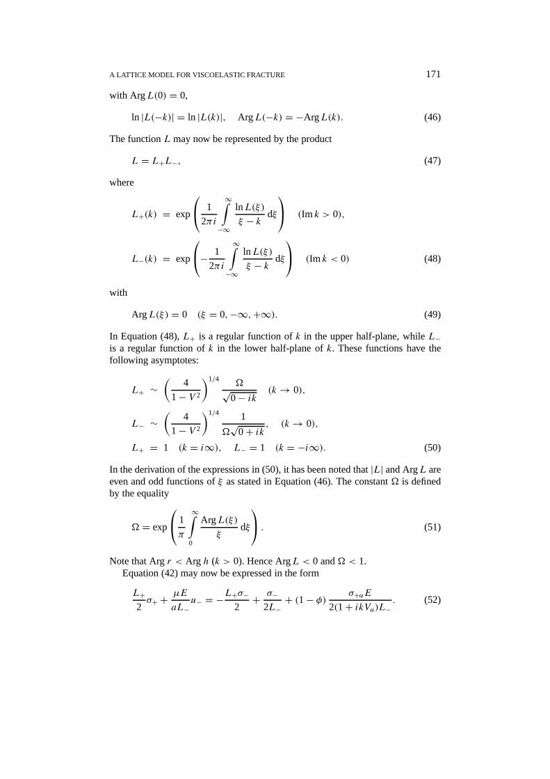
Figure 4. Effective energy release ratiosversusvelocity for a range ofCα = αc/a values,given thatφ = 0.9.
Figure 5. Effective energy release ratiosversusvelocity for a range ofCα = αc/a values,given thatφ = 0.1.
words, the wave resistance increases and hence slow crack growth is possible.This is one of the most important phenomena exhibited by this viscoelastic latticemodel. An increase in the relaxation time,β, leads to the elastic-type behaviorof the energy release ratio, while an increase in the creep time,α, results insuppression of the dynamic effects.

A LATTICE MODEL FOR VISCOELASTIC FRACTURE 177
Figure 6. Effective energy release ratiosversuslog10(αc/a) for a range ofv/c values, giventhatφ = 0.1.
Figure 7. Energy release ratio for the elastic lattice (φ = 1)
3.1. TRANSITION TO A HOMOGENEOUSMATERIAL
The Fourier-description of the problem for a homogeneous material follows fromthat for the lattice as an asymptote fork → 0, by the substitution ofk2/2 for1− cosk in h2 and 4E for r2; E equalsE under the condition thata = 1 (underthese conditionk becomes the dimensional parameter of the Fourier transformationoverx). In addition, the second term in the expression foru− in (61) is negligiblein comparison with the first term because it is finite while the first term isO(k−3/2)
if k → 0. Note that this term represents the crack opening displacements whicharise due to the extension of the bonds between the particles on the linesn = 0 and
178 L.I. SLEPYAN ET AL.
n = −1 in front of the crack. In the classical formulation for a homogeneous body,there is no such layer and there is no corresponding term. Thus
E = 1+ ikαv1+ ikβv ,
h2 = Ek2+ (0+ ikV )2,
L = 2
√E
h, L+ = 1√
0− ik ,
σ+(k) = C1√0− ik , C1 = const,
L− = 2
(1+ iαvk
1− V 2+ ikv(α − βV 2)
)1/2 1√0+ ik ,
u−(k) = C1/E
(0+ ik)3/2(
1+ iαvk1− V 2+ ikv(α − βV 2)
)1/2
. (72)
In the case of a homogeneous material, the expression for the energy release rateat the moving crack tip corresponds to an elastic body with the short term modulusbecause the stress/strain rates tend to infinity in the vicinity of the crack tip and isgiven by (Slepyan, 1990)
G0 = limp→∞p
2σ+(ip)u−(−ip) = C21
φ√1− V 2φ
. (73)
The far-field energy release rateG is given by the long-wave approximation (k→0) and corresponds to an elastic material loaded under the same conditions. FromEquation (73), under the condition thatα = β,
G = C21√
1− V 2. (74)
Note that this expression coincides with that in Equation (65). Thus the energyrelease ratioG0/G is given by
R0 = G0
G= φ
√1− V 2
1− V 2φ. (75)
Note that this ratio depends onφ = α/β but notα andβ separately. This conclu-sion, however, is valid only for a homogeneous viscoelastic material but not for alattice.

A LATTICE MODEL FOR VISCOELASTIC FRACTURE 179
3.2. TRANSITION TO AN ELASTIC LATTICE
Let 0< Vβ < Vα → 0. In this case, it follows from Equation (57) thatL+α → 1.Now the relations (67–70) become as follows:
σ (+0) = �√2G, ε(+0)→ �√
2G,
Gv
G→ Ge
G→ G0
G→ �2. (76)
At the same time,E → 1 (so long as|k| does not tend to infinity), and hence thefunction� defined by Equation (51) tends to that based onE = 1. Thus, in contrastto a homogeneous viscoelastic material, the results for a viscoelastic lattice tend tothose for the elastic lattice when the creep and relaxation times,α andβ, tendto zero. This conclusion is not unexpected. Indeed, in the case of a homogeneousviscoelastic material there is no time-unit besidesα andβ, and hence the associatedenergy release ratios can depend only on the ratio of these parameters. In contrast,a lattice model harbors a time-unit associated with the structure, and an elasticlattice retains a limit with respect to ratios of the creep and relaxation times to thistime-unit.
Note that for an elastic lattice, the ratios considered in Equation (76) are in-dependent of the elastic modulusµ/a. It manifests itself only in the dependence�(V ).
3.3. QUASI-STATIC LIMIT
For a homogeneous material, Equation (75) provides that
R0 = G0
G= β
α(v = +0). (77)
Thus in a viscoelastic homogeneous material, there is a finite dissipation even for avanishing crack velocity. This is a manifestation of the fact that the energy releaseat a moving crack tip corresponds to an elastic body with the glassy modulus, whilethe far field corresponds to the low-rate modulus.
In contrast, the quasi-static limit of the local energy release for a viscoelasticlattice obviously corresponds to an elastic lattice. Indeed, in the case of a largetime-interval between the breakage of two neighboring bonds, the influence ofviscosity on the lattice state has time to vanish. Thus, dissipation does not changethe final strain energy of the bond before it breaks, and this energy is the same as inthe elastic lattice. In this quasi-static case, the resistance caused by viscosity in theviscoelastic lattice is the same as the wave resistance in the elastic lattice. It can bedetermined by the formula (Slepyan, 1982a)
R0 = exp
− 1
π
π∫0
lnL(k)dk
(v = +0, ArgL = 0), (78)

180 L.I. SLEPYAN ET AL.
where the functionL for the discrete Fourier transformation overx is the same asfor the continuous transformation fort = 0 (see Appendix 3).
In the case of the square-cell lattice,
R0 = exp
− 1
2π
π∫0
ln4+ 2(1− cosk)
2(1− cosk)dk
= √2− 1. (79)
3.4. VISCOELASTIC LATTICE WITH α ≥ β = 0
As first pointed out by Kostrov and Nikitin (1970), for crack propagation in aviscoelastic homogeneous material with 0= β < α, the energy release at thepropagating crack tip is zero. This can be easily seen in Equation (75). This effectis a consequence of the fact that in this case the short term modulus is infinite. Adifferent conclusion is reached via a viscoelastic lattice model. Indeed, in the caseof a lattice, the glassy modulus does not play such a dramatic role, and ifβ = 0,Equations (63), (67) and (68) give
σ (+0) = �√2Gµ, ε(+0) = �
L+α
√2G
µ(80)
and the energy release ratio (69) is still nonzero as are the ratios in (70).
3.5. VISCOELASTIC LATTICE WITH vα →∞, α/β = CONST
For a given 0< V < 1, whenVα →∞, the functionL+α in Equation (57) behavesas
L+α ∼[
4
1− V 2
]1/4√Vα�→∞ (81)
and hence (see Equation (70))
Re ∼ φ2�2, R0 ∼ φ�2. (82)
To proceed, represent the integrand in (51) as the sum∞∫
0
ArgL(ξ)
ξdξ = Iel+ Ihv,
Iel =∞∫δ
ArgL(ξ)
ξdξ,
Ihv =δ∫
0
ArgL(ξ)
ξdξ, δ→ 0, Cαδ→∞, (83)

A LATTICE MODEL FOR VISCOELASTIC FRACTURE 181
whereIhv andIel denote the ‘homogeneous viscoelastic’ and ‘elastic lattice’ por-tions, respectively. InIel, one may replaceE by α/β. With δ small inIhv, one mayreplace 2(1− cosk) by k2 andr2 by 4E. That is,
Iel ∼∞∫
0
ArgL(ξ)dξ
ξ
(E = α
β
),
Ihv = 1
2
δ∫0
Arg1+ iξVα
1− V 2+ iξ(Vα − V 2Vβ)
dξ
ξ
∼ 1
2
∞∫0
Arg1+ iξ
1− V 2+ i(1− V 2φ)ξ
dξ
ξ
= π
4ln
1− V 2
1− V 2φ. (84)
Now
�el = exp(Iel/π), �hv = exp(Ihv/π) =(
1− V 2
1− V 2φ
)1/4
. (85)
The integralIel corresponds to an elastic lattice with the instantaneous modulus:
Rel = �2el
(E = α
β
), (86)
while Ihv, corresponds to a homogeneous viscoelastic material (see Equations (82)and (75)),
Rhv = φ√
1− V 2
1− V 2φ= φ�2
hv. (87)
The energy release ratio for a homogeneous viscoelastic material is portrayedin Figure 8.
Under the conditions considered here, the function� in (51) may now berepresented via the product
� = �el�hv (88)
and hence
σ (+0) = �el�hv
√2Gµ, ε(+0) = φ�el�hv
√2G/µ. (89)
Since the second term in the last expression forAv in (21) tends to zero forVα → 0,it follows that
Re ∼ φRelRhv, Rv ∼ R0 ∼ RelRhv. (90)

182 L.I. SLEPYAN ET AL.
Figure 8. Energy release ratioversusvelocity for a homogeneous viscoelastic material.
A natural separation of the lattice and viscosity effects has now been obtained.Note that this case (Vα → ∞ with φ = const) corresponds to a large viscosity aswell as a small size of the lattice cell under given viscosity. Indeed, an increase ofthe parametersVα andVβ is equivalent to a decrease of the lattice cell size.
For finite steady-state crack speeds, the viscous resistance to crack propagationis high if the ratioα/β is large. At the same time, the quasi-static limit correspondsto the elastic lattice case which is independent of viscosity. Evidently, a pronouncedinfluence of viscosity on the resistance to crack propagation in a lattice is possible:the resistance increases very fast with crack velocity in the low velocity regime.
The above separation may be useful even in numerical simulations of vis-coelastic fracture based on a lattice model. When the crack speed variabilitycorresponds to a large viscosity time-scale, the lattice effect can be separated andthe coupling with a homogeneous viscoelastic material model becomes transparent.
4. Lattice Strip
Consider now a square-cell lattice strip. Let the particles on the linesn = N andn = −N − 1 be fixed (see Figure 9). At the crack surfacesη < 0, an externalloading,±q = const, is expected to act on the particlesn = 0 and−1, respectively.The crack propagates between the linesn = 0 andn = −1 and the displacementfield is anti-symmetric. In the case of this clamped strip
uFn = uF0λn − λ2N−n
1− λ2N(n ≥ 0),
uFn = −uF0λ−1−n − λ2N+1+n
1− λ2N(n ≤ −1). (91)

A LATTICE MODEL FOR VISCOELASTIC FRACTURE 183
Figure 9. A square-cell clamped lattice strip.
The same dynamic equations (30) and (39) govern the deformations, where
σ− = −q = const (η < 0). (92)
The following expression for the Fourier transform ofσm follows from Equa-tions (39) and (91),
σ+ = q− − µa[(h2+ E)uF − EuF1 ]
= q− − µh
2aω1(u+ + u−), (93)
in which
q− = qF = q
0+ ik , ω1 = (r + h)2N − (r − h)2N(r + h)2N+1+ (r − h)2N+1
. (94)
Substituting foru+ in Equation (93) by the expression in (11), an equation identicalto (42) is obtained, but with a different expression for the functionL:
L = rω2
h= 4Eω1
h+ 1, ω2 = (r + h)2N+1− (r − h)2N+1
(r + h)2N+1+ (r − h)2N+1. (95)
In contrast to the unbounded lattice, the coefficient,L/(2E), and the right partof Equation (42) are now meromorphic functions: they do not contain branchpoints. Indeed
L = D1
D2(96)

184 L.I. SLEPYAN ET AL.
with
D1 =N∑m=0
(2N + 1
2m+ 1
)(r2)N−m(h2)m,
D2 =N∑m=0
(2N + 1
2m
)(r2)N−m(h2)m, (97)
where(N
m
)is a binomial coefficient(0≤ m ≤ N). Further
L→ 1 (k→ ±∞), L→ 2N + 1 (k→ 0), IndL = 0. (98)
The last equality follows from the inequality (37) which shows that Reω2 > 0. Atthe same time,ω2→ 1 (k → ±∞). The trajectory forω2 in the complexk-planeis closed and the pointk = 0 lies outside the area enclosed by this trajectory.
Equation (42) can now be rewritten in the form (52)
L+2σ+ + µE
aL−u−
= q
2(0+ ik)(L+ − 1
L−
)+ (1− φ) σ+α
2(1+ ikVβ)L− , (99)
whereL+ andL− are defined by Equations (48) and (96). For the lattice strip, thelatter decomposition gives the following asymptotic expressions:
L+(k)→ 1 (k→+i∞),L−(k)→ 1 (k→−i∞),L+(k)→
√2N + 1� (k→ 0),
L−(k)→√
2N + 1/� (k→ 0),
� = exp
1
π
∞∫0
ArgL(ξ)
ξdξ
. (100)
The first term on the right-hand side of Equation (99) must be expressed as thesum of two terms, one regular in the upper half-plane and one regular in the lowerhalf-plane (remembering thatE = E−). This is done as follows:
q
2(0+ ik)(L+ − 1
L−
)= C+ + C−,
C+ = q[L+(k)− L+(0)]2(0+ ik) , C− = q
2(0+ ik)(L+(0)− 1
L−(k)
). (101)

A LATTICE MODEL FOR VISCOELASTIC FRACTURE 185
The solution of Equation (99) is now given by
σ+ = q
0+ ik(
1− L+(0)L+(k)
),
u− = qa
2µE(0+ ik) [L+(0)L−(k)− 1] + (1− φ) σ+α2(1+ ikVα) . (102)
Subsequently (compare with (14)),
σ (+0) = limp→∞pσ+(ip) = q[L+(0)− 1],
ε(+0) = 2u(0)
a= 2
alimp→∞pu−(−ip)
= q
µ
{φ[L+(0)− 1] + (1− φ)
[L+(0)L+α
− 1
]},
u(−∞) = limp→0
pu−(−ip) = qaN/µ. (103)
The global energy release rate can be defined as the total work of the traction minusthe elastic energy per unit length of the lattice strip far to the left of the crack tip.It is
G = 2[qu(−∞)− qu(−∞)/2] = q2N/µ. (104)
For the clamped lattice strip, the energy release ratios are given by
R0 = 1
2N(9 − 1)
[φ(9 − 1)+ (1− φ)
(9
L+α− 1
)],
Re = 1
2N
[φ(9 − 1)+ (1− φ)
(9
L+α− 1
)]2
,
9 = √2N + 1�. (105)
These expressions tend to the corresponding expressions in (70) for the unboundedlattice whenN →∞.
5. Quasi-Static Behavior
For both the unbounded lattice and the lattice strip, the case of slow steady-statecrack propagation (v � c) is considered. In fact, the asymptotic behavior is ex-amined forV → 0 without restrictions respective to the parameterVα: it can tendto zero, a nonzero value, or infinity. In this case, in the determination of the energyrelease ratios, the inertia of the lattice can be neglected because the correspondingterm tends to zero for any finitek.

186 L.I. SLEPYAN ET AL.
The functionL(k) has a static limit forV → 0 which is independent of thecreep and relaxation timesα andβ. In the limiting case, it is a periodic, nonnegativefunction, and the periodT = 2π . The factorization of a Cauchy-type integral fora periodic function is required in this case. Eatwell and Willis (1982) and Slepyan(1982a) showed that any nonnegative, periodic, locally integrable functionL(k)
may be factorized as follows (ArgL = 0), withL = L+L−,
L±(k) = exp
± 1
2iT
T/2∫−T/2
InL(ξ) cotπ(ξ − k)
Tdξ
, (106)
where Imk > 0 for L+ and Imk < 0 for L−, respectively;T is the period. Thelimiting values are (noting thatL(−ξ) = L(ξ))
L+(k) → L+∞ (k→ i∞),L−(k) → L+∞ (k→−i∞),
L+∞ = exp
1
T
T/2∫0
InL(ξ)dξ
, (107)
and
L+α = exp
1
2iT
T/2∫−T/2
InL(ξ) cotπ
T
(ξ − i
Vα
)dξ
. (108)
The expressions in (61) are unmodified.For the unbounded square-cell lattice, the functionL in Equation (106) can be
re-expressed in the form
L =(
4+ 2(1− cosk)
2(1− cosk)+ 0
)1/2
=(
1+ sin2 k/2
sin2 k/2+ 0
)1/2
. (109)
For this function, the following explicit factorization is valid:
L+ =[
sin(k/2+ iArsh 1)
sin(k/2+ i0)]1/2
=[√
2 sink/2+ i cosk/2
sin(k/2+ i0)
]1/2
,
L− =[
sin(k/2− iArsh 1)
sin(k/2− i0)]1/2
=[√
2 sink/2− i cosk/2
sin(k/2− i0)
]1/2
. (110)
Note that this factorization differs from that derived above in Equation (48) in spiteof the fact that the functionL in Equation (109) is the limit of that defined by

A LATTICE MODEL FOR VISCOELASTIC FRACTURE 187
Equation (43) forV → 0. The asymptotes ofL± are
L+ ∼√
2
0− ik , L− ∼√
2
0+ ik (k→ 0),
L+ ∼√√
2+ 1 (k→ i∞),
L− ∼√√
2− 1 (k→−i∞), (111)
and
L+α =(√
2+ coth1
2Vα
)1/2
. (112)
On the basis of these results and the general solution in (61), the far-field stressis given by
σ+ ∼ C√2(0− ik) . (113)
From this it follows that
KIII = C/√a, C = √2Gµ. (114)
The Fourier transforms of the stress and crack opening displacement can now beexplicitly written in terms of the far-field energy release rate:
σ+α = Vα√
2Gµ
L+α,
σ+ =√
2Gµ
0− ik[
sin(k/2+ i0)√2 sink/2+ i cosk/2
]1/2
,
u− = a
2E
√2G/µ
0+ ik
[√2 sink/2− i cosk/2
sin(k/2− i0)
]1/2
+ a (1− φ) σ+α2µ(1+ ikVα) . (115)
Note that only the crack opening displacement depends on the crack speed (dueto the presence of the second term); the stresses do not. By neglecting inertia, thestress distribution is independent of viscosity.
Displacement continuity is not maintained in the vicinity of a crack tip amassless viscoelastic lattice:
u(+0) 6= u(−0). (116)
In this case, the limiting strain of the breaking bond is defined by the formula in(14) only.

188 L.I. SLEPYAN ET AL.
The limiting stress, strain and displacement discontinuity are
σ (+0) = ϑ√
2Gµ,
ε(+0) = ϑZ√
2G/µ,
u(−0)− u(+0) = limk→−i∞
(iku−)− aε(+0)/2= aϑφ√G/µ (117)
in which
ϑ =√√
2− 1,
Z = φ + (1− φ)[(√
2− 1)
(√2+ coth
1
2Vα
)]−1/2
. (118)
For the slow steady-state fracture of an unbounded viscoelastic lattice, theenergy release ratios are
Re = Ge
G= (√2− 1)Z2, R0 = G0
G= (√2− 1)Z. (119)
Each ratio approaches the value√
2 − 1 at zero crack velocity (compare withEquation (79)).
These results, derived independently of the dynamic treatment, present exactquasi-static asymptotes for low crack velocities (V � 1) in an unbounded lattice,valid for any value of the parameterVα. While the dynamic asymptote forV →0, and the quasi-static solution itself are different, the difference manifests itselfjust after the breakage of a bond. Then, due to a large time-interval between thebreakage of neighboring bonds, the dynamic state quickly approaches the quasi-static state. When the parameterVα � 1 the energy release ratios
Re ∼ R0 ∼ (√
2− 1). (120)
However, if it happens thatV � 1, Cα � 1, φ � 1, such that for a small increasein the crack velocity the parameterVα becomes large, these same ratios are muchreduced
Re ∼ (√
2− 1)φ2, R0 ∼ (√
2− 1)φ. (121)
This reduction, which correlates with an increase in the resistance to crack propaga-tion, occurs over a small portion of the steady-state crack speed regime. Thus, inthis model, the speed of a slowly propagating crack will depend very strongly onthe applied load or the far-field energy release rate. In these considerations, it hasbeen assumed that a stable crack obeys a criterion likeG0 ≤ Gc, yet in the case ofa slowly propagating crack, it is the same as a limiting strain criterion:ε(+0) ≤ εc.
Consider now the case of slow steady-state crack propagation (v � c) in aclamped square-cell lattice strip. The quasi-static solution may be deduced based

A LATTICE MODEL FOR VISCOELASTIC FRACTURE 189
on the formulas (102) and (14) forσ+ andε+, respectively, and by noting (96–97),with
L = D1s
D2s,
3 = sin2 k/2+ 0
1+ sin2 k/2,
D1s =N∑m=0
(2N + 1
2m+ 1
)3m,
D2s =N∑m=0
(2N + 1
2m
)3m. (122)
In this case,
L+(0) =√
2N + 1,
L+α → L+∞ (Vα → 0),
L+α → L+(0) (Vα →∞) (123)
and
σ (+0) = q(√2N + 1/L+∞ − 1), ε(+0) = qZ1/µ. (124)
in which
Z1 = φ(√
2N + 1
L+∞− 1
)+ (1− φ)
(√2N + 1
L+α− 1
). (125)
For the slow steady-state fracture of an clamped viscoelastic lattice, the energyrelease ratios are
Re = Z21/2N, R0 = (
√2N + 1/L+∞ − 1)Z1/2N. (126)
These ratios have the following asymptotes:
Re ∼ R0 ∼ (√
2N + 1/L+∞ − 1)2/2N (Vα → 0),
Re ∼ φ2(√
2N + 1/L+∞ − 1)2/2N (Vα →∞),R0 ∼ φ(
√2N + 1/L+∞ − 1)2/2N, (Vα →∞). (127)

190 L.I. SLEPYAN ET AL.
6. Discussion
The role of the discrete structure of the lattice and the dimensionless viscoelasticparametersVα = αv/a andφ = β/α are shown in Figures 2–7. From the macro-level point of view, both the radiation by high-frequency waves due to the structureresponse and dissipation itself can be called ‘dissipation’. The latter quantity isthe difference between the total energy release,G, as the energy flux from infinityand the energy lost in the breaking bonds,G0. For these plots, the latter energy isdefined in terms of the limiting tensile force and strain:G0 = σ (+0)ε(+0)/2 andthe ratio,R0 = G0/G, is shown.
The curveφ = 1 shown in Figure 2 corresponds to an elastic lattice (shownseparately in Figure 7). The dependence forφ = 1 is characterized by the followingdistinctive features. The dissipation is finite for a vanishing crack speed:R0(0) =√
2−1. This is due to radiation by high-frequency waves which are excited by eachbreak of the bond. In the presence of viscosity (φ < 1), these waves dissipate butthe long-wave energy flux from infinity does not (sincev = +0), and this initialpoint,R0(0), is the same for any dissipation. Next,R0 possesses a maximum foreach value ofφ (if φ is not too low), and hence the dissipation (by this radiation)has a minimum at approximately half the shear wave speed (v/c ≈ 1/2). Further,R0 has a nonmonotone dependence on crack speed for lowv/c values. This is amanifestation of a strong dependence on the number of different waves, and theenergy which they carry away from the propagating crack tip, on the crack speed.Finally, the energy release ratio tends to zero and hence the resistance to crackpropagation increases without bound as the crack speed approaches the shear wavespeed. As can be seen in Figure 2, the influence of viscosity increases shouldφ =β/α decrease further; this results in a monotonic increase of the resistance over thewhole crack speed range (0< v/c < 1).
An influence ofCα = αc/a on the considered dependencies forφ = 0.5,0.9and 0.1 are presented in Figures 3, 4 and 5, respectively. The viscosity has almostno influence forφ = 0.9 (Figure 4), cannot prevent the nonmonotonic behaviorwhen φ = 0.5 (Figure 3), and has a strong influence in the case ofφ small(Figure 5). The influence ofCα for some values of the crack speed in the lattercase is shown in Figure 6.
The energy release ratio for a homogeneous viscoelastic material is portrayedin Figure 8. In contrast to a lattice, the result here depends onφ only and there isno pronounced increase of the resistance to crack propagation over an initial regionof the crack speed. Hence slow crack growth cannot occur within the frameworkof a homogeneous viscoelastic material model.
The role of the discrete structure of the lattice strip, and the nondimensionalparametersVα andφ, and the strip width is shown in Figures 10–15. In each figure,the curves differ by the parameterN which characterizes the strip width,(2N+1)a.These plots correspond toφ = 0.5 andCα = 0.1, 1, 2, 10 and 100 in Figures 10,11, 12, 13 and 14, respectively. The results for the elastic lattice strip are presented

A LATTICE MODEL FOR VISCOELASTIC FRACTURE 191
Figure 10. Effective energy release ratioversus velocity for the lattice strip withCα = 0.1, φ = 0.5.
Figure 11. Effective energy release ratioversus velocity for the lattice strip withCα = 1, φ = 0.5.
in Figure 15. Forφ = 0.5, an increase inCα does not eliminate the nonmonotonicbehavior of the energy release ratioversuscrack speed. Also, the lattice strip resultsdiffer from those for the unbounded lattice even for rather large values ofN . Atthe same time, qualitatively, the plots forN = ∞ andN = 10 are similar. Theseconclusions are important as regards the interpretation of numerical modeling usinglattice strips of finite width. The energy release ratio decreases with a decreaseof the strip width (considering that the bond length,a, remains the same). The
192 L.I. SLEPYAN ET AL.
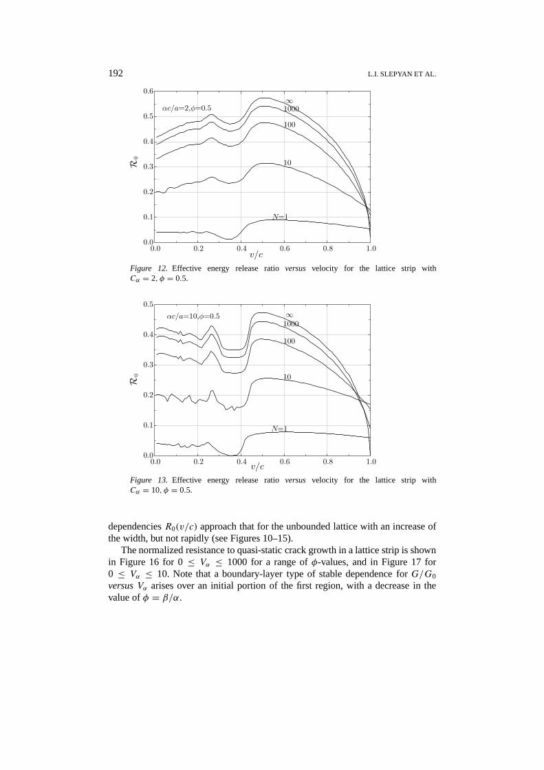
Figure 12. Effective energy release ratioversus velocity for the lattice strip withCα = 2, φ = 0.5.
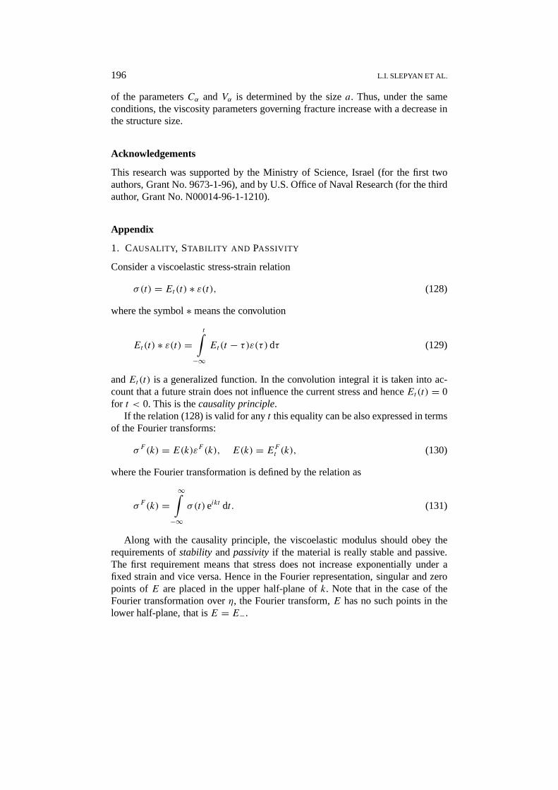
Figure 13. Effective energy release ratioversus velocity for the lattice strip withCα = 10, φ = 0.5.
dependenciesR0(v/c) approach that for the unbounded lattice with an increase ofthe width, but not rapidly (see Figures 10–15).
The normalized resistance to quasi-static crack growth in a lattice strip is shownin Figure 16 for 0≤ Vα ≤ 1000 for a range ofφ-values, and in Figure 17 for0 ≤ Vα ≤ 10. Note that a boundary-layer type of stable dependence forG/G0
versusVα arises over an initial portion of the first region, with a decrease in thevalue ofφ = β/α.

A LATTICE MODEL FOR VISCOELASTIC FRACTURE 193
Figure 14. Effective energy release ratioversus velocity for the lattice strip withCα = 100, φ = 0.5.
Figure 15. Energy release ratios for the elastic lattice strip (φ = 1).
7. Conclusions
In this paper, the main aspects of steady-state crack propagation in a square-cellviscoelastic lattice have been studied. In an elastic lattice, there is structure butno viscosity. In viscoelastic homogeneous and cohesive-zone models, there is vis-cosity but no material structure. In this viscoelastic lattice model, there are bothmaterial structure and viscosity. Coupling the latter two factors causes a diversearray of crack propagation phenomena. As shown, these factors can be separatedin the case of pronounced viscosity,Cα = cα/a → ∞, φ = β/α = const.

194 L.I. SLEPYAN ET AL.
Figure 16. Normalized resistance to quasi-static crack growth in a lattice stripversus0≤ Vα ≤ 1000 for a range ofφ-values.
Figure 17. Normalized resistance to quasi-static crack growth in a lattice stripversus0≤ Vα ≤ 10 for a range ofφ-values.
No dynamic effects such as radiation given steady-state crack propagation exist inthe cohesive zone models. Also, the lattice differs (from cohesive zone models)by a regular structure, the same in the crack path and in the bulk of the material.This creates no artificial restrictions on the crack-speed-dependent distribution ofdissipation caused by viscosity.
The dynamic viscoelastic lattice model reduces to the requisite quasi-static limitand homogeneous viscoelastic material behavior. The first limit coincides withthe static state. However, during slow crack growth, radiation still occurs because

A LATTICE MODEL FOR VISCOELASTIC FRACTURE 195
of discrete bond-rupture events. In the homogeneous material case, an importantboundary-layer-type dependence, which is revealed by the lattice model in the caseof pronounced viscosity, is lost as follows: in a viscoelastic lattice, the rapid rise inresistance for early crack acceleration allows slow cracks to grow stably. Formally,this phenomenon manifests itself in a very rapid rise in the value ofVα = vα/a
due solely to a small increase of the normalized crack speedV = v/c from v = 0(if the parameterCα is large). In homogeneous materials,Vα = ∞ for anyv > 0becausea = 0, and this physically important behavior cannot be modeled.
In contrast to an elastic lattice, the high-frequency waves cannot propagate asoscillations of the lattice structure in the viscoelastic lattice from infinity becauseof dissipation due to viscosity. The only structure-associated waves which exist areexcited by the propagating crack. For moderate viscosity, the amount of energycarried away from the crack tip by these waves decreases with an increase of thecrack speed (for slow crack speeds). In this case, slow crack growth is not possible.With increasing viscosity, that is, for an increase ofCα given thatφ is low, theresistance by viscosity increases and the role of the radiation resistance becomesless important. The latter observation, however, does not concern the zero-speedlimit where the influence of high frequency wave radiation on the resistance tocrack propagation remains important.
The solutions derived in this paper give the relations between the global (far-field) and local energy release rates, and relations between the far-field energyrelease rate and the breaking bond strain. These crack-speed and viscosity-dependent relations can be used for the crack propagation determination undergiven conditions and fracture criterion. However, in the formulation adopted in thispaper, the crack speed is prescribed and the energy release ratios are consideredunder a given speed. In general, to come to a conclusion whether a steady-statesolution exists, and if it does, at what crack speed one has to invoke a material-dependent fracture criterion and to trace whether it is satisfied by the solution (overeach successive time-interval from one periodic bond-fracture to the next). Theanalysis shows, in particular, that for large viscosity the limiting strain consideredis maximal at the end of each such time-interval. Were one to use the limitingstrain criterion as a fracture criterion, the solutions derived in this paper could beused to determine the associated crack speed. This observation applies equally toslow stable crack growth.
Note that the lattice model can also be looked upon as a finite-element ap-proximation of a continuous material. Numerical simulations of this type oflattice model, including various nonlinear extensions, requires no additional finite-element approximation. On the other hand, the analytical solutions derived for theinfinite lattice and lattice strip, and phenomena revealed by this model, can serveas benchmark solutions for finite-element analyses.
Finally, the solutions derived are expressed in terms of nondimensional para-metersCα = αc/a, Vα = αv/a andφ. This suggests a structure-associated sizeeffect. Indeed, for given relaxation and creep times and the crack speed, the size
196 L.I. SLEPYAN ET AL.
of the parametersCα andVα is determined by the sizea. Thus, under the sameconditions, the viscosity parameters governing fracture increase with a decrease inthe structure size.
Acknowledgements
This research was supported by the Ministry of Science, Israel (for the first twoauthors, Grant No. 9673-1-96), and by U.S. Office of Naval Research (for the thirdauthor, Grant No. N00014-96-1-1210).
Appendix
1. CAUSALITY, STABILITY AND PASSIVITY
Consider a viscoelastic stress-strain relation
σ (t) = Et(t) ∗ ε(t), (128)
where the symbol∗means the convolution
Et(t) ∗ ε(t) =t∫
−∞Et(t − τ)ε(τ)dτ (129)
andEt(t) is a generalized function. In the convolution integral it is taken into ac-count that a future strain does not influence the current stress and henceEt(t) = 0for t < 0. This is thecausality principle.
If the relation (128) is valid for anyt this equality can be also expressed in termsof the Fourier transforms:
σF (k) = E(k)εF (k), E(k) = EFt (k), (130)
where the Fourier transformation is defined by the relation as
σF (k) =∞∫−∞
σ (t)eikt dt. (131)
Along with the causality principle, the viscoelastic modulus should obey therequirements ofstability andpassivityif the material is really stable and passive.The first requirement means that stress does not increase exponentially under afixed strain and vice versa. Hence in the Fourier representation, singular and zeropoints ofE are placed in the upper half-plane ofk. Note that in the case of theFourier transformation overη, the Fourier transform,E has no such points in thelower half-plane, that isE = E−.

A LATTICE MODEL FOR VISCOELASTIC FRACTURE 197
The feature of passivity means that work cannot be negative, that is
A =t∫
0
σ (t)ε dt ≥ 0
(ε = dε
dt
). (132)
Consider a closed path of strain:ε = 0 for t < 0 andt > T <∞. In this case, theParseval equality can be used in the form
A =T∫
0
σ (t)ε dt = 1
2π
∞∫−∞
E(k)εF (k)(ε)F (k)dk
= 1
2π
∞∫−∞
E(k)ik|εF (k)|2 dk = − 1
π
0∫−∞
ImE(k)|εF (k)|2k dk
= − 1
π
∞∫0
ImE(k)|εF (k)|2k dk. (133)
It follows from this that for a passive material
Im kE(k) ≤ 0. (134)
Note that this inequality is changed for the opposite one in the case of the Four-ier transformation overη. For the above-considered constitutive equation (1),Equation (134) leads to the inequalityα ≥ β.
2. GENERALIZED STANDARD MODEL
Consider a more general one-dimensional force-strain relation for a viscoelasticbond:∏
n
(1+ βn d
dt
)σ =
∏n
(1+ αn d
dt
)ε, 1≤ n ≤ n∗. (135)
Here, note the restriction that no two values amongαn, βn are the same. For asteady-state problem in which the considered functions depend onη only, thisrelation takes the form∏
n
(1− Vβn d
dη
)σ =
∏n
(1− Vαn d
dη
)ε. (136)
Using the right-sided Fourier transformation it can be found that
σ+∏n
(1+ ikVβn)− 2u+∏n
(1+ ikVαn) =∑n
ankn−1, (137)

198 L.I. SLEPYAN ET AL.
where the polynomial of the powern∗ − 1 in the right part arises as a result of thistransformation; it depends on values ofσ (+0) andu(0) and their derivatives up tothe ordern∗ − 1. The constantsan are defined by the requirement thatσ+ andu+do not contain poles and zeros in the upper half-plane ofk, i.e., they really can bemarked by the subscript+. These conditions are satisfied by the expressions
σ+(k) = 2
∏n(1+ ikVαn)∏n(1+ ikVβn)
u+(k)
− 2n∗∑m=1
∏n(1− αn/βm)u+[i/Vβm]
(1+ ikVβm)∏n6=m(1− βn/βm),
u+(k) =∏n(1+ ikVβn)
2∏n(1+ ikVαn)
σ+(k)
−n∗∑m=1
∏n(1− βn/αm)σ+[i/Vαm]
2(1+ ikVαm)∏n6=m(1− αn/αm). (138)
In the simplest casen∗ = 1,∏n6=m = 1, and the relation in (11) is obtained.
3. CONTINUOUS AND DISCRETEFOURIER TRANSFORMS
Consider a functionf (x−vt), x = an, n = 0,±1, . . .. The Fourier transformationover(−vt/a) leads to
f (−vt/a)(k)
=∞∫−∞
f (x − vt)eikη−ikn d(−vt/a) = e−iknf F (k), (139)
where
f F (k) =∞∫−∞
f (η)eikη dη, η = (x − vt)/a. (140)
The discrete Fourier transform of (139) is
g(k, q) =∞∑
n=−∞f (−vt/a) eiqn = 2πf F (k)δ(k − q), (141)
whereδ is the Dirac delta-function.The discrete Fourier transform off follows from using the inverse transforma-
tion of (141) overk:
f n(q) = 1
2π
∞∫−∞
g(k, q)eikvt/a dk = f F (q)eiqvt/a. (142)

A LATTICE MODEL FOR VISCOELASTIC FRACTURE 199
In the problems considered in this paper, the discrete Fourier transform is neededfor t = 0, when the limiting stress and strain are achieved in the bond with thecoordinatex = 0. For this time the discrete and continuous transformations giveus the same result:
f n(q) = f F (q). (143)
4. CAUSALITY PRINCIPLE FORSTEADY-STATE SOLUTIONS
A steady-state solution for a domain unbounded in thex-direction can be non-unique due to the existence of one or a set of inherent solutions as free waves whichcan be considered as produced by sources at infinity. The existence of such wavesreflects itself by singular and zero points on the realk-axis of the Fourier transformsof the steady-state solutions. If such sources are not allowed by the problem for-mulation, they must be excluded from the solution. This can be achieved in variousways, in particular by the use of a rule based on the causality principle. Under thisprinciple, the steady-state solution is considered as a limit (timet → ∞) of thesolution to the corresponding transient problem with zero initial conditions.
Consider the inverse Laplace (with respect to timet) and Fourier (with respectto the coordinatex) transformations, and let it beuLF (s, k), of a functionu(t, x)
u(t, x) = 1
2π
1
2πi
∞∫−∞
i∞+0∫−i∞+0
uLF (s, k)est−ikx ds dk. (144)
The solution is required to become steady-state in the coordinate system movingalong thex-coordinate with velocityv, that is in the coordinateη = x − vt .Substitutex = η + vt in the representation (144), giving
u(t, x) = w(t, η)
= 1
2π
1
2πi
∞∫−∞
i∞+0∫−i∞+0
uLF (s, k)e(s−ikv)t−ikη ds dk. (145)
Now denotes = ikv + p, wherek is assumed to be real, Rep = +0:
w(t, η) = 1
2π
1
2πi
∞∫−∞
i∞+0∫−i∞+0
uLF (p + ikv, k)ept−ikη dp dk. (146)
The last equality is the inverse Laplace transform (with respect to the explicitlywritten t) and Fourier transform (with respect toη) transformations ofwLF(p, k) =uLF (p + ikv, k) of the originalw(t, η). From this it follows that the doubletransformation in the moving coordinate system is
wLFη(p, k) = uLF (p + ikv, k). (147)

200 L.I. SLEPYAN ET AL.
It is assumed that a limit of the functionw(t, η) exists whent →∞, η = const.The well-known limiting theorem states:
If a limit of a functionf (t) with t →∞ exists, it is
limt→∞f (t) = lim
p→0pf L(p), (148)
wheref L(p) is the Laplace transform off (t). For our problem this means that
limt→∞w
Fη(t, k) = limp→+0
puLF (p + ikv, k). (149)
However, if a nonzero limit exists, its Laplace transform contains the multiplier1/p as for each constant original. Thus the causality-principle-based rule states:
For a steady-state solution, in the Fourier transform corresponding to the movingcoordinate system, each productikv must be supplemented by the term+0 whichmeans the limit from the right.
This makes the solution uniquely defined. Mathematically, it makes the realk-axisfree of the singular and zero points.
References
Atkinson, C. and List, R.D., ‘A moving crack problem in a viscoelastic solid’,Internat. J. Engrg. Sci.10, 1972, 309–322.
Atkinson, C. and Popelar, C.H., ‘Antiplane dynamic crack propagation in a viscoelastic strip’,J.Mech. Phys. Solids27, 1979, 431–439.
Bažant, Z.P. and Jirásek, M., ‘R-curve modeling of rate and size effects in quasibrittle fracture’,Internat. J. Fracture62, 1993, 355–373.
Bažant, Z.P. and Li, Y.-N., ‘Cohesive crack model with rate-dependent crack opening and viscoelasti-city: I. Mathematical model and scaling’,Internat. J. Fracture86, 1997, 247–265.
Bažant, Z.P. and Planas, J.,Fracture and Size Effect in Concrete and Other Quasibrittle Materials,CRC Press, Boca Raton, FL, 1998.
Costanzo, F. and Walton, J.R., ‘A study of dynamic crack growth in elastic materials using a cohesivezone model’,Internat. J. Engrg. Sci.35, 1997, 1085–1114.
Costanzo, F. and Walton, J.R., ‘Numerical simulations of a dynamically propagating crack with anonlinear cohesive zone’,Internat. J. Fracture91, 1998, 373–389.
Eatwell, G.P. and Willis, J.R., ‘The Excitation of a fluid-loaded plate stiffened by a semi-infinitearray of beams’,IMA J. Appl. Mech.29(3), 1982, 247–270.
Fineberg, J., Gross, S.P., Marder, M. and Swinney, H.L., ‘Instability in dynamic fracture’,Phys. Rev.Lett.67(4), 1991, 457–460.
Fineberg, J., Gross, S.P., Marder, M. and Swinney, H.L., ‘Instability in the propagation of fast cracks’,Phys. Rev. B45(10), 1992, 5146–5154.
Freund, L.B.,Dynamic Fracture Mechanics, Cambridge University Press, Cambridge, 1990.Geubelle, P.H., Daniluk, M.J. and Hilton, H.H., ‘Dynamic mode III fracture in viscoelastic media’,
Int. J. Solids Structures35, 1998, 761–782.Herrmann, J.M. and Walton, J.R., ‘A comparison of the dynamic transient antiplane shear crack
energy release rate for standard linear solid and power law type viscoelastic materials’,ASME J.Energy Res. Tech.113, 1991, 222–229.

A LATTICE MODEL FOR VISCOELASTIC FRACTURE 201
Herrmann, J.M. and Walton, J.R., ‘On the energy release rate for dynamic transient mode 1 crackpropagation in a general viscoelastic body’,Quart. Appl. Math.52, 1994, 201–228.
Hillerborg, A., Modéer, M. and Petersson, P.E., ‘Analysis of crack formation and crack growth inconcrete by means of fracture mechanics and finite elements’,Cem. & Concrete Res.6, 1976,773–782.
Kanninen, M.F. and Popelar, C.H.,Advanced Fracture Mechanics, Oxford University Press, Oxford,1985.
Knauss, W.G., ‘Delayed failure – The Griffith problem for linearly viscoelastic materials’,Internat.J. Fracture6, 1970, 7–20.
Knauss, W.G., ‘The mechanics of polymer fracture’,Appl. Mech. Rev.26, 1973, 1–17.Knauss, W.G., ‘On the steady propagation of a crack in a viscoelastic sheet: experiments and ana-
lysis’, in Deformation and Fracture of High Polymers, H.H. Kausch, J.A. Hassel and R.I. Jaffe(eds.), Plenum Press, New York, 1974, 501–541.
Knauss, W.G., ‘Fracture of solids possessing deformation rate sensitive material properties’, inDe-formation and Fracture of High Polymers, H.H. Kausch, J.A. Hassel and R.I. Jaffe (eds.), PlenumPress, New York, 1976, 501–541.
Knauss, W.G., ‘The mechanics of polymer fracture’, inApplied Mechanics Update, C.R. Steele andG.S. Springer (eds.), ASME, New York, 1986, 211–216.
Knauss, W.G., ‘Time dependent fracture of polymers’, inAdvances in Fracture Research, Vol. 4, K.Salama, K. Ravi-Chandar, D.M.R. Taplin and P. Rama Rao (eds.), Pergamon Press, New York,1989, 2683–2711.
Knauss, W.G., ‘Time dependent fracture and cohesive zones’,J. Engrg. Mat. & Tech.115, 1993,262–267.
Knauss, W.G. and Dietmann, H., ‘Crack propagation under variable load histories in linearlyviscoelastic solids’,Internat. J. Engrg. Sci.8, 1970, 643–656.
Knauss, W.G. and Mueller, H.K., ‘On the governing equations for quasi-static crack growth inlinearly viscoelastic materials’,ASME J. Appl. Mech.42, 1975, 520–521.
Kostrov, B.V. and Nikitin, L.V., ‘Some general problems of mechanics of brittle fracture’,Arch.Mech. Stos.22, 1970, 749–775.
Kulakhmetova, Sh.A., ‘Influence of anisotropy of a lattice on an energy outflow from a propagatingcrack’,Vestnik LGU22, 1985a, 51–57 [in Russian].
Kulakhmetova, Sh.A., ‘Dynamics of a crack in an anisotropic lattice’,Sov. Phys. Dokl.30(3), 1985b,254–255.
Kulakhmetova, Sh.A., Saraikin, V.A. and Slepyan, L.I., ‘Plane problem of a crack in a lattice’,Mech.Solids19(3), 1984, 101–108.
Langer, J.S. and Lobkovsky, A.E., ‘Critical examination of cohesive-zone models in the theory ofdynamic fracture,’J. Mech. Phys. Solids46, 1998, 1521–1556.
Lee, O.S. and Knauss, W.G., ‘Dynamic crack propagation along a weakly bonded plane in apolymer’,Exp. Mech.29, 1989, 342–345.
Li, V.C. and Liang, E., ‘Fracture processes in concrete and fiber reinforced cementitious composites’,ASCE J. Engrg. Mech. Div.112, 1986, 566–586.
Marder, M., ‘New dynamical equation for cracks,Phys. Rev. Lett.66, 1991, 2484–2487.Marder, M. and Gross, S., ‘Origin of crack tip instabilities’,J. Mech. Phys. Solids43, 1995, 1–48.Marder, M. and Xiangmin Liu, ‘Instability in lattice fracture’,Phys. Rev. Lett.71(15), 1993, 2417–
2420.Mikhailov, A.M. and Slepyan, L.I., ‘Steady-state motion of a crack in a unidirectional composite’,
Mech. Solids21(2), 1986, 183–191.Mueller, H.K. and Knauss, W.G., ‘Crack propagation in a linearly viscoelastic strip’,J. Appl. Mech.
38, 1971, 483–488.Mulmule, S.V. and Dempsey, J.P., ‘Stress-separation curve for saline ice using the fictitious crack
model’,ASCE J. Engrg. Mech.123, 1997, 870–877.

202 L.I. SLEPYAN ET AL.
Mulmule, S.V. and Dempsey, J.P., ‘A viscoelastic fictitious crack model for the fracture of sea ice’,Mech. Time-Dependent Mater.1, 1998, 331–356.
Nuismer, R.J., ‘On the governing equations for quasi-static crack growth in linearly viscoelasticmaterials’,ASME J. Appl. Mech.41, 1974, 631–634.
Popelar, C.H. and Atkinson, C., ‘Dynamic crack propagation in a viscoelastic strip’,J. Mech. Phys.Solids28, 1980, 79–93.
Ryvkin, M. and Banks-Sills, L., ‘Steady-state mode iii propagation of an interface crack in aninhomogeneous viscoelastic strip’,Internat. J. Solids and Structures30, 1992, 483–498.
Ryvkin, M. and Banks-Sills, L., ‘Mode III delamination of a viscoelastic strip from a dissimilarviscoelastic half-plane’,Internat. J. Solid and Structures31, 1994, 551–566.
Schapery, R.A., ‘A theory of crack initiation and growth in viscoelastic media I. Theoreticaldevelopment’,Internat. J. Fracture11, 1975a, 141–159.
Schapery, R. A., ‘A theory of crack initiation and growth in viscoelastic media II. Approximatemethod of analysis’,Internat. J. Fracture11, 1975b, 369–388.
Schapery, R.A., ‘A theory of crack initiation and growth in viscoelastic media III. Analysis ofcontinuous growth’,Internat. J. Fracture11, 1975c, 549–562.
Sills, L.B. and Benveniste, Y., ‘Steady state propagation of a mode III interface crack in aninhomogeneous viscoelastic media’,Internat. J. Engrg. Sci.19, 1981, 1255–1268.
Slepyan, L.I., ‘Dynamics of a crack in a lattice’,Sov. Phys. Dokl.26, 1981a, 538–540.Slepyan, L.I., ‘Crack propagation in high-frequency lattice vibrations’,Sov. Phys. Dokl.26(9), 1981b,
900–902.Slepyan, L.I., ‘Antiplane problem of a crack in a lattice’,Mech. Solids17(5), 1982a, 101–114.Slepyan, L.I., ‘The relation between the solutions of mixed dynamic problems for a continuous elastic
medium and a lattice’,Sov. Phys. Dokl.27(9), 1982b, 771–772.Slepyan, L.I., ‘Dynamics of brittle fracture in media with a structure’,Mech. Solids19(6), 1984,
114–122.Slepyan, L.I., ‘Dynamics of brittle fracture in media with a structure – Inhomogeneous problems’, in
Mathematical Methods of Mechanics of Solids, R.V. Goldstein and O.A. Oleinik (eds.), Nauka,Moscow, 1986, 143–149 [in Russian].
Slepyan, L.I.,Mechanics of Cracks, 2nd edition, Sudostroenie, Leningrad, 1990 [in Russian].Slepyan, L.I., ‘Role of microstructure in fracture and phase transition dynamics’, inMECAMAT’93:
International Seminar on Micromechanics of Materials, Editions EYROLLES, Moret-sur-Loing,France, 1993, 246–257.
Slepyan, L.I., ‘Crack dynamics’, inFracture: A Topical Encyclopedia of Current Knowledge Ded-icated to Alan Arnold Griffith, G. Cherepanov (ed.), Krieger Publishing Company, Melbourne,U.S.A., 1998, 620–661.
Slepyan, L.I. and Kulakhmetova, Sh.A., ‘Crack propagation in a bed consisting of rigid blocks withelastic interlayers’,Phys. Solid Earth22(12), 1986, 977–982.
Slepyan, L.I. and Troyankina, L.V., ‘Fracture wave in a chain structure’,J. Appl. Mech. Techn. Phys.25(6), 1984, 921–927.
Slepyan, L.I. and Troyankina, L.V., ‘Shock waves in a nonlinear chain’, inStrength and Visco-plasticity, R.V. Gol’dstein (ed.), Nauka, Moscow, 1988, 301–305 [in Russian].
Walton, J.R., ‘On steady-state propagation of anti-plane shear crack in an infinite general linearlyviscoelastic body’,Quart. Appl. Math.40, 1982, 37–52.
Walton, J.R., ‘The dynamic energy release rate for a steadily propagating antiplane shear crack in alinear viscoelastic body’,J. Appl. Mech.54, 1987, 635–641.
Walton, J.R., ‘Dynamic viscoelastic fracture’, inCrack and Contact Problems for ViscoelasticBodies, G.A.C. Graham and J.R. Walton (eds.), Springer-Verlag, Wien, 1995, 259–311.
Walton, J.R. and Herrmann, J.M., ‘A new method for solving dynamically accelerating crack prob-lems: Part 1. The case of a semi-infinite mode III crack in elastic material revisited’,Quart. Appl.Math.50, 1992, 373–387.

A LATTICE MODEL FOR VISCOELASTIC FRACTURE 203
Williams, M.L., ‘The fracture of viscoelastic material’, inFracture of Solids, D.C. Drucker and J.J.Gilman (eds.), Interscience Publishers, 1962, 157–188.
Willis, J.R., ‘Crack propagation in viscoelastic media’,J. Mech. Phys. Solids15, 1967a, 229–240.Willis, J.R., ‘A comparison of the fracture criteria of Griffith and Barenblatt’,J. Mech. Phys. Solids
15, 1967b, 151–162.Wnuk, M.P. and Knauss, W.G., ‘Delayed fracture in viscoelastic-plastic solids’,Internat. J. Solids
and Structures6, 1970, 995–1009.Wu, Z.S. and Bažant, Z.P., ‘Finite element modeling of rate effect in concrete fracture with influence
of creep’, inCreep and Shrinkage of Concrete, Z.P. Bažant and I. Carol (eds.), E & FN Spon,London, 1993, 424–432.