A Lyapunov Formulation of Nonlinear Small Gain Theorem forInterconnected ISS Systems� yZhong-Ping Jiangz, Iven M. Y. Mareelsx and Yuan Wang{Submitted to AutomaticaRevised January 20, 1996Abstract. The goal of this paper is to provide a Lyapunov statement and proof of the recentnonlinear small-gain theorem for interconnected input/state stable (iss) systems. An iss-Lyapunovfunction for the overall system is obtained from the corresponding Lyapunov functions for both thesubsystems.Keywords. Interconnected systems, nonlinear gain, Lyapunov function, stability.1 IntroductionThe notion of nonlinear gains has recently been acknowledged of interest by a number of authors.Its use in generalizing the classical small (�nite) gain theorem for nonlinear feedback systems waspointed out in Hill (1991) and Mareels and Hill (1992) within the input-output context. A similaridea of nonlinear gains was also introduced in the independent work of Sontag (1989, 1990, 1995) in astate-space setting. Recently, the authors of (Jiang et al. 1994) have combined the idea of nonlineargains from the above two di�erent areas and established an L1 version of the nonlinear small gaintheorem in which the role of the initial conditions is made explicit and asymptotic stability (in theLyapunov sense) for the internal states is included. Related results and applications of the nonlinearsmall-gain theorem in nonlinear robust stability and nonlinear stabilization have been pursued in(Jiang 1993, Jiang et al. 1994, Praly and Jiang 1993, Jiang and Mareels 1995, Teel and Praly toappear, Lin et al. to appear, Praly and Wang 1994). These studies are based on the concept of gainfunctions. It is well known that Lyapunov functions play an important role in analysis and design of�The preliminary version of this paper was presented at the IFAC Symposium on Nonlinear Control Systems Designwhich was held in Tahoe City, California during 25-28 June 1995. Corresponding author Z.-P. Jiang's Telephone +616 249 2461; Fax +61 6 279 8088; Email zjiang@syseng.anu.edu.au.yThe work of Z.-P. Jiang and I. Mareels were supported in part by the funding of the activities of the CRC forRobust and Adaptive Systems by the Australian Government under the Cooperative Research Centers program. Thework of Y. Wang was supported in part by NSF Grants DMS-9457826 and DMS-9403924.zDepartment of Systems Engineering, Australian National University, Canberra ACT 0200, AUSTRALIA.xDepartment of Engineering, FEIT, Australian National University, ACT 0200, AUSTRALIA.{Department of Mathematics, Florida Atlantic University, Boca Raton, FL 33431, USA.1

nonlinear dynamical systems, and it is therefore natural to ask whether these nonlinear small-gainresults can be derived using Lyapunov-like arguments.In this paper, we report on some preliminary results in this direction. The main contribution ofthe paper is to establish a Lyapunov-type nonlinear small-gain theorem whose proof relies upon theconstruction of appropriate Lyapunov functions.The layout of the paper is as follows. We start with some mathematical preliminaries in whichwe introduce the basic de�nitions and recall some results. The main result is stated and illustratedin Section 3. Section 4 is devoted to the proof of the main result. We conclude in Section 5. Theappendix contains some technical lemmas used in the main proof.2 Mathematical Preliminaries2.1 NotationWe employ j � j to denote the usual Euclidean norm for vectors and k � k to denote the L1 norm fortime functions. For a real-valued di�erentiable function V , rV stands for its gradient. xT is thetransposition of the vector x 2 IRn.2.2 isps-Lyapunov functionsBefore stating our main theorem in Section 3, we introduce in this section some stability notions andsome basic results.Consider the following controlled dynamical system :_x = f(x; u) (1)where x 2 IRn , u 2 IRm , and f : IRn� IRm ! IRn is a locally Lipschitz map. Controls are measurableessentially bounded functions from IR+ to IRm .Recall that a function : IR+ ! IR+ is of class K if it is continuous, strictly increasing and (0) = 0. It is of class K1 if, in addition, it is unbounded. A function � : IR+ � IR+ ! IR+ is ofclass KL if, for each �xed t, the function �(�; t) is of class K and, for each �xed s, the function �(s; �)is decreasing and tends to zero at in�nity.De�nition 2.1 (Jiang et al. 1994, Jiang 1993) The system (1) is said to be input-to-state practicallystable (isps) if there exist a function � of class KL, a function of class K and a nonnegativeconstant d such that, for each initial condition x(0) and each measurable essentially bounded controlu(�) de�ned on [0;1), the solution x(�) of system (1) exists on [0;1) and satis�es :jx(t)j � �(jx(0)j; t) + (kuk) + d 8t � 0 (2)When (2) is satis�ed with d = 0, the system (1) is said to be input-to-state stable (iss), a notionoriginally introduced by Sontag (1989, 1990).De�nition 2.2 A smooth (i.e., C1) function V is said to be an isps-Lyapunov function for system(1) if 2

� V is proper, positive de�nite, that is, there exist functions 1, 2 of class K1 such that 1(jxj) � V (x) � 2(jxj); 8 x 2 IRn : (3)� there exist a positive-de�nite function �, a class K function � and a nonnegative constant csuch that the following implication holds:njxj � �(juj) + co =) rV (x) f(x; u) � ��(jxj) : (4)When (4) holds with c = 0, V is called an iss-Lyapunov function for system (1).Remark 2.3 Observe that this de�nition is slightly di�erent from the original de�nition proposedby Sontag and Wang (1995a) in that � is only required to be positive de�nite rather than class Kas in (Sontag and Wang 1995a). The equivalence of both de�nitions can be shown, see also Remark4.2 in (Lin et al. to appear).Remark 2.4 One can de�ne the isps-Lyapunov function in a slightly di�erent way. Instead ofrequiring (4) holds for V , one asks the following holds for V :rV (x)f(x; u)� �a(V (x)) + �(juj) + d (5)for some functions a 2 K1, � 2 K, and some constant d � 0. Correspondingly, one asks d = 0 in (5)for V to be an iss-Lyapunov function.It is immediate that system (1) admits an isps- (resp. iss)-Lyapunov function satisfying (3)-(4)if and only if it admits an isps- (resp. iss)-Lyapunov function satisfying (3) and (5), cf. (Sontag andWang 1995a).Recently, the equivalence between the isps property and the existence of an isps-Lyapunov func-tion was shown in (Sontag and Wang 1995b), i.e.:Proposition 2.5 The system (1) is isps (resp. iss) if and only if it has an isps- (resp. iss)-Lyapunovfunction.3 Main ResultThe main purpose of this section is to derive a Lyapunov-type nonlinear small-gain theorem, ratherthan gain functions based small-gain theorem as in (Jiang et al. 1994, Jiang 1993), for interconnectedsystems : _x1 = f1(x1; x2; u1) (6)_x2 = f2(x1; x2; u2) (7)where, for i = 1; 2, xi 2 IRni , ui 2 IRmi , and fi : IRn1 � IRn2 � IRmi ! IRni is locally Lipschitz.Assume that, for i = 1; 2, there exists an isps-Lyapunov function Vi for the xi-subsystem suchthat the following holds: 3

1. there exist functions i1; i2 2 K1 so that i1(jxij) � Vi(xi) � i2(jxij) ; 8 xi 2 IRni : (8)2. there exist functions �i 2 K1, �i; i 2 K and some constant ci � 0 so that V1(x1) �maxn�1(V2(x2)); 1(ju1j) + c1o impliesrV1(x1) f1(x1; x2; u1) � ��1(V1) (9)and V2(x2) � maxn�2(V1(x1)); 2(ju2j) + c2o impliesrV2(x2) f2(x1; x2; u2) � ��2(V2): (10)In the following we will give a nonlinear small-gain condition under which an isps-Lyapunov functionfor the interconnected system (6)-(7) may be expressed in terms of isps-Lyapunov functions for thetwo subsystems.Theorem 3.1 Assume that, for i = 1; 2, the xi-subsystem has an isps-Lyapunov function Vi satis-fying (8), (9) and (10). If there exists some c0 � 0 such that�1 � �2(r) < r ; 8 r > c0 ; (11)then the interconnected system (6)-(7) is isps. Furthermore, if c0 = c1 = c2 = 0, then the system isiss. In particular, the zero solution of (6)-(7) with no input (i.e. u = 0) is globally asymptoticallystable.Remark 3.2 Condition (11) is equivalent to�2 � �1(r) < r ; 8 r > c0 (12)where c0 � 0, and c0 = 0 if and only if c0 = 0.Proof: Assume that (11) holds. De�nec0 = supfr : �2 � �1(r) � rg : (13)First notice that, with (11), we have :�2 � �1(r) < r ; 8 r 2 (�2(c0); �2(1)): (14)From this it follows that c0 � �2(c0). Therefore (12) follows from (13) readily.By symmetry, one knows that if (12) holds, then (11) holds with c0 � �1(c0). 2Remark 3.3 If V1 and V2 are isps-Lyapunov functions for the subsystems satisfying (8), andrV1(x1) f1(x1; x2; u1) � �a1(V1(x1)) + �x1(V2(x2)) + �u1 (ju1j) + d1 ; (15)rV2(x1) f2(x1; x2; u2) � �a2(V2(x2)) + �x2(V1(x1)) + �u2 (ju2j) + d2 (16)4

for some ai 2 K1, �xi ; �ui 2 K and di � 0 (i = 1; 2), then �1, �2 can be chosen as�1(r) = a�11 � (Id + ") � �x1(r)�2(r) = a�12 � (Id + ") � �x2(r)for any " > 0, where Id stands for the identity function: Id(r) = r for all r. Thus, condition (11)becomes that there exist " > 0 and r0 � 0 such thata�12 � (Id + ") � �x2 � a�11 � (Id + ") � �x1 (r) < r; 8 r � r0 : (17)Corollary 3.4 If, for i = 1; 2, Vi is an isps-Lyapunov function of the xi-subsystem satisfying (8),(15) and (16) with �x1(s) = �1 a2(s) ; �x2(s) = �2 a1(s)for some �1 > 0 and �2 > 0, then condition (17) is satis�ed if �1�2 < 1. So the conclusion ofTheorem 3.1 holds.Note that Corollary 3.4 may be seen as an extension of (Gruji�c and �Siljak 1973, Theorem 1) in thecase of two subsystems. Also note that, in this case, the composite functions �1V1(x1) + �2V2(x2)form a family of smooth isps-Lyapunov functions for the overall system, provided that �1 > 0, �2 > 0and �1�1 < �2 < �1=�2.Remark 3.5 It is of interest to note that condition (11) is very similar to the so-called nonlinearsmall-gain conditions utilized in (Jiang et al. 1994, Jiang 1993, Teel and Praly to appear). In fact,in our case, �1 or a�11 � (Id + ") � �x1 (resp. �2 or a�12 � (Id + ") � �x2 ) may be seen as an input-outputgain (Jiang et al. 1994, Jiang and Mareels 1995) for the x1 (resp. x2) subsystem with V2 (resp. V1)as input and V1 (resp. V2) as output.In order to illustrate the usefulness of Theorem 3.1 in testing the global asymptotic stability ofnonlinear systems, we give an elementary example.Example 3.6 Consider the three-dimensional nonlinear system :_z1 = �z1 + z31z2_z2 = �z2 � z61z2 + z23_z3 = �z33 + 0:5jz1j 32 (18)Let x1 = (z1 z2)T and x2 = z3. As it can be directly checked, V1(x1) = 12z21 + 12z22 is an iss-Lyapunovfunction for the x1-subsystem of (18) with x2 as input and gains in (4) of the form�1(r) = 83� 2"1 r2for su�ciently small "1 > 0. Also, V2(x2) = 12x22 is an iss-Lyapunov function for the x2-subsystem of(18) with x1 as input and gains in (4) of the form�2(r) = 2 13(4� "2) 23 r 12for su�ciently small "2 > 0. Simple calculation shows that there exist su�ciently small "1 > 0, "2 > 0such that �1 � �2(r) < r for all r > 0, namely condition (11) holds with c0 = 0. Therefore, fromTheorem 3.1, it follows that the system (18) is globally asymptotically stable at (z1; z2; z3) = (0; 0; 0).5

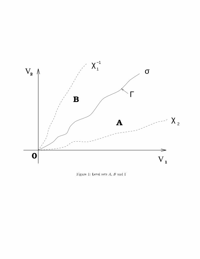
4 Proof of Theorem 3.1To simplify the proof of Theorem 3.1, the following observation is useful.Lemma 4.1 For any �1, �2, c1 and c2 satisfying (9)-(10), if (11) holds with c0 > 0, then we canalways choose e�1, e�2, ec1 and ec2 such that (9), (10) are satis�ed and (11) holds with ec0 = 0. Inaddition, ec1 = ec2 = 0 if c0 = c1 = c2 = 0.Proof: Let c� = 2c0 and pick any K1-function e�2 with the property that e�2(r) = �2(r) for all r � c�,and �1 � e�2(r) < r for all r > 0 (this is always possible because �1 � e�2(r) = �1 � �2(r) < r forall r � c�). With the new gain function e�2, it holds that �2(r) � maxfe�2(r); �2(c�)g. By (10), itfollows that rV2(x2)f2(x1; x2; u) � ��2(V2) whenever V2(x2) � maxne�2(V1(x1)); 2(ju2j) + ~c2o,where ec2 = c2 + �2(c�) = c2 + �2(2c0).De�ning e�1 = �1 and ec1 = c1 ends the proof. 2Proof of Theorem 3.1 : In the light of Lemma 4.1, we may assume, without loss of generality, thatc0 = 0 in (11). Denote b = limr!1�1(r) (19)(note that b =1 if �1 2 K1). Then ��11 is de�ned on [0; b), ��11 (r)!1 as r! b�, and�2(r) < ��11 (r) ; 8 r 2 (0; b) :Now we let b�1 be a function of K1 such that� b�1(r) � ��11 (r) for each r 2 [0; b);� �2(r) < b�1(r) for all r > 0.(Note that one can let b�1(r) = ��11 (r) if �1 2 K1.) Applying Lemma A.1 in the appendix to �2 andb�1, one sees that there exists a K1-function � continuously di�erentiable on (0; 1) with �0(r) > 0for all r > 0 such that �2(r) < �(r) < b�1(r); 8 r > 0 :Now we de�ne V (x1; x2) = maxn�(V1(x1)); V2(x2)o : (20)Clearly V is proper and positive de�nite. Also note that �(V (x1)) is locally Lipschitz on IRn1 n f0g,and V2 is locally Lipschitz everywhere. It is then a standard fact that V is locally Lipschitz onIRn n f0g where n = n1 + n2. Therefore, V is di�erentiable almost everywhere (a.e.).Let f(x; u) = (f1(x1; x2; u1)T ; f2(x1; x2; u2)T )T and u = (uT1 ; uT2 )T . In the following we showthat there exist a positive de�nite function �, a K-function and a constant c � 0 such that thefollowing implication holds:nV (x) � (juj) + co =) rV (x) f(x; u) � ��(V (x)) ; a: e: (21)To this purpose, we de�ne the following sets, as shown in Figure 1:A = n(x1; x2) : V2(x2) < �(V1(x1))o ;B = n(x1; x2) : V2(x2) > �(V1(x1))o ;� = n(x1; x2) : V2(x2) = �(V1(x1))o :6

Now �x any point p = (p1; p2) 6= (0; 0), and a control value v = (v1; v2). There are three cases:Case 1: p 2 A. In this case V (x1; x2) = �(V1(x1)) in a neighborhood of p, and consequently,rV (p)f(p; v) = �0(V1(p1))rV1(p1) f1(p1; p2; v1) : (22)For p 2 A, it holds that V2(p2) < �(V1(p1)), and therefore, V1(p1) > �1(V2(p2)). This then impliesrV1(p1)f1(p1; p2; v1) � ��1(V1(p1))whenever V1(p1) � 1(jv1j) + c1. From this it follows that for p 2 A,rV (p)f(p; v)� �b�1(V (p)) (23)whenever V (p) � �( 1(jv1j) + c1), where b�1 is a positive de�nite function given byb�1(s) = �0(��1(s))�1(��1(s)) 8s > 0: (24)We now let b 1(r) = �( 1(r + c1))� �( 1(c1)); (25)and let bc1 = �( 1(c1)). Then (23) becomesrV (p) f(p; v)� �b�1(V (p)) ; (26)whenever V (p) � b 1(jv1j) + c1.Case 2: p 2 B. Using exactly the same arguments as in Case 1, one shows that in this case,rV (p) f(p; v) � ��2(V (p)) ; (27)whenever V (p) � 2(jv2j) + c2.Case 3: p 2 �. First note that for the locally Lipschitz function V , it holds thatrV (p) f(p; v) = ddt ����t=0 V ('(t)); a: e:;where '(t) = ('1(t); '2(t)) is the solution of the initial value problem_'(t) = f('(t); v); '(0) = p :Assume p = (p1; p2) 6= (0; 0) is such thatV1(p1) � 1(jv1j) + c1; (28)V2(p2) � 2(jv2j) + c2 : (29)It then holds that r�(V1(p1)) f1(p1; p2; v1) � �b�1(V (p));rV2(p2) f2(p1; p2; v2) � ��2(V (p)):7

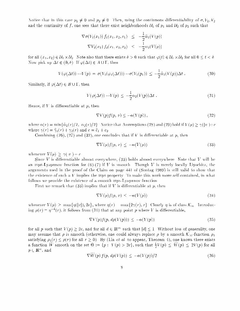
Notice that in this case p1 6= 0 and p2 6= 0. Then, using the continuous di�erentiability of �; V1; V2and the continuity of f , one sees that there exist neighborhoods U1 of p1 and U2 of p2 such thatr�(V1(x1)) f1(x1; x2; v1) � �12 b�1(V (p))rV2(x2) f2(x1; x2; v2) � �12�2(V (p))for all (x1; x2) 2 U1�U2. Note also that there exists � > 0 such that '(t) 2 U1�U2 for all 0 � t < �.Now pick up �t 2 (0; �). If '(�t) 2 A [ �, thenV ('(�t))� V (p) = �(V1('1(�t)))� �(V1(p1)) � �12 b�1(V (p))�t : (30)Similarly, if '(�t) 2 B [ �, thenV ('(�t))� V (p) � �12�2(V (p))�t : (31)Hence, if V is di�erentiable at p, thenrV (p)f(p; v) � ��(V (p)) ; (32)where �(r) = minfb�1(r)=2; �2(r)=2g. Notice that Assumptions (28) and (29) hold if V (p) � (jvj)+cwhere (r) = b 1(r) + 2(r) and c = bc1 + c2.Combining (26), (27) and (32), one concludes that if V is di�erentiable at p, thenrV (p)f(p; v) � ��(V (p)) (33)whenever V (p) � (jvj) + c.Since V is di�erentiable almost everywhere, (33) holds almost everywhere. Note that V will bean isps-Lyapunov function for (6)-(7) if V is smooth. Though V is merely locally Lipschitz, thearguments used in the proof of the Claim on page 441 of (Sontag 1989) is still valid to show thatthe existence of such a V implies the isps property. To make this work more self-contained, in whatfollows we provide the existence of a smooth isps-Lyapunov function.First we remark that (33) implies that if V is di�erentiable at p, thenrV (p)f(p; v) � ��(V (p)) (34)whenever V (p) � maxf�(jvj); 2cg, where �(r) = maxf2 (r); rg. Clearly � is of class K1. Introduc-ing �(r) = ��1(r), it follows from (34) that at any point p where V is di�erentiable,rV (p)f(p; d�(V (p))) � ��(V (p)) (35)for all p such that V (p) � 2c, and for all d 2 IRm such that jdj � 1. Without loss of generality, onemay assume that � is smooth (otherwise, one could always replace � by a smooth K1-function �1satisfying �1(r) � �(r) for all r � 0). By (Lin et al. to appear, Theorem 4), one knows there existsa function fW smooth on the set � := fp : V (p) > 2cg, such that 12V (p) � fW (p) � 2V (p) for allp 2 IRn , and rfW (p) f(p; d�(V (p)) � ��(V (p))=2 (36)8

for all p 2 �, and all jdj � 1. To get an isps-Lyapunov function that is smooth everywhere, one�nds a smooth, proper and positive de�nite function W such that W (p) = fW (p) for all p such thatV (p) > ec for any ec > 2c. For such a choice of W , it holds thatrW (p) f(p; d�(V (p)) � ��(V (p))=2 (37)for all p such that V (p) � ~c, all jdj � 1, which implies that rW (p) f(p; v) � ��(V (p))=2 for all(p; v) such that V (p) � ��1(jvj) and V (p) � ec. Since both W and V are positive de�nite and proper,there exist a positive de�nite function ��, a K-function � and a constant �c � 0 such that there holdsthe following implication:nW (p) � � (jvj) + �co =) rW (p) f(p; v) < ���(W (p)) : (38)Finally note that if c1 = c2 = c0 = 0, then (36) holds for all p 6= 0 and all jdj � 1. Then onecan directly apply (Lin et al. to appear, Proposition 4.2) to fW and f to get a smooth, proper andpositive de�nite function W such that (37) holds for all p 6= 0 and jdj � 1. With this, one gets (38)with �c = 0. Hence, V and W provide iss-Lyapunov functions for the system. 25 ConclusionIn this short paper, we gave an alternative proof of the so-called nonlinear small gain theorem forinterconnected iss systems by means of iss-Lyapunov function arguments. An iss-Lyapunov functionfor the total system is generated from the corresponding iss-Lyapunov functions for the subsystems.The key technique was to modify appropriately the gain function (i.e. � in (4)) for each subsystem.It complements the techniques of changing supply functions in a di�erential dissipation inequality(cf. (5)) proposed in the recent contribution (Sontag and Teel 1995) for single iss systems.ReferencesGruji�c, L. T. and D. D. �Siljak (1973). Asymptotic stability and instability of large-scale systems.IEEE Transactions on Automatic Control, 18, 636{645.Hill, D. J. (1991). A generalization of the small-gain theorem for nonlinear feedback systems. Auto-matica, 27(6), 1047{1050.Jiang, Z. P. (1993). Quelques R�esultats de Stabilisation Robuste. Application �a la Commande. PhDthesis. �Ecole des Mines de Paris.Jiang, Z. P. and I. M. Y. Mareels (1995). Robust control of time-varying nonlinear cascaded systemswith dynamic uncertainties. European Control Conference (ECC'95), pp. 659-664, Roma, Italy.Jiang, Z. P., A. Teel and L. Praly (1994). Small-gain theorem for ISS systems and applications.Mathematics of Control, Signals, and Systems, 7, 95-120.Lin, Y., E. D. Sontag and Y. Wang (to appear). A smooth converse Lyapunov theorem for robuststability. SIAM Journal on Control and Optimization. (Preliminary version in \Recent resultson Lyapunov-theoretic techniques for nonlinear stability", in Proc. Amer. Automatic ControlConference, Baltimore, June 1994, pp. 1771-1775.).9

Mareels, I. M. Y. and D. J. Hill (1992). Monotone stability of nonlinear feedback systems. Journalof Mathematical Systems Estimation Control, 2, 275{291.Praly, L. and Z. P. Jiang (1993). Stabilization by output feedback for systems with ISS inversedynamics. Systems and Control Letters, 21, 19-34.Praly, L. and Y. Wang (1994). Stabilization in spite of matched unmodelled dynamics and an equiv-alent de�nition of input-to-state stability. Submitted to MCSS.Sontag, E. D. (1989). Smooth stabilization implies coprime factorization. IEEE Trans. Automat.Control, 34, 435{443.Sontag, E. D. (1990). Further facts about input to state stabilization. IEEE Trans. Automat. Control,35, 473{476.Sontag, E. D. (1995). State-space and i/o stability for nonlinear systems. In: Feedback Control,Nonlinear Systems, and Complexity, Lecture Notes in Control and Information Sciences (B. A.Francis and A. R. Tannenbaum, Eds.). Springer-Verlag.Sontag, E. D. and A. Teel (1995). Changing supply functions in input/state stable systems. IEEETrans. Automat. Control, 40, 1476-1478.Sontag, E. D. and Y. Wang (1995a). On characterizations of the input-to-state stability property.Systems & Control Letters, 24, 351-359.Sontag, E. D. and Y. Wang (1995b). On characterizations of set input-to-state stability. In: Prep.IFAC Nonlinear Control Systems Design Symposium (NOLCOS '95), pp. 226-231, Tahoe City,CA.Teel, A. and L. Praly (to appear). Tools for semi-global stabilization by partial state and outputfeedback. SIAM Journal on Control and Optimization.Appendix{Technical LemmasThe following technical lemma is used in the proof of Theorem 3.1.Lemma A.1 Let �1 2 K and �2 2 K1 satisfying �1(r) < �2(r) for all r > 0. Then there exists aK1-function � such that� �1(r) < �(r) < �2(r) for all r > 0;� �(r) is C1 on (0; 1), and �0(r) > 0 for all r > 0.Before proving this lemma, we �rst give an intermediate result.Lemma A.2 Let �0 : [0; 1)! [0; 1) be a continuous function such that �0(0) = 0 and �0(r) > 0for all r > 0. Then there exists a continuous function � : [0; 1)! [0; 1) such that� �(r) < �0(r) for all r > 0; 10

� � is C1 on (0; 1), and �0(r) � 1=2 for all r > 0.Proof : We may assume that �0(r) � 1=2 for all r � 0. Otherwise use minf1=2; �0(r)g to replace�0(r). Let �1(r) = 8><>: mins2[r;2]�0(s) ; if 0 � r � 1,mins2[1;r+1]�0(s) ; if r > 1:Note then that �1 is not increasing on (1; 1), and not decreasing on (0; 1). Also note that �1(r) ��0(r) for all r � 0, and �1(r� 1) � �0(r) for all r � 1. To get a desired function �, we let�(r) = 8>><>>: Z r0 �1(s) ds if 0 � r � 1,Z rr�1 �1(s) ds if r > 1:It is easy to see that � is continuously di�erentiable, and �0(r) � �1(r) � 1=2 for all r > 0. Observethat �(r) � r�1(r) � �0(r) for r 2 [0; 1]; �(r) � �1(r � 1) � �0(r) for r � 2. Furthermore, forr 2 (1; 2), it holds that �(r) = Z 1r�1 �1(s) ds+ Z r1 �1(s) ds� �1(1)(2� r) + �1(1)(r� 1)= �1(1) � �0(r) :Hence, � has all the desired properties. 2Now, we return to prove Lemma A.1.Proof of Lemma A.1 : Let �0(r) = r� ��12 � �1(r)2 :Then ��12 � �1(r) < r � �0(r), and consequently,�1(r) < �2(r � �0(r)) ; 8 r > 0 :By Lemma A.2, one knows that there exists a function � such that 0 < �(r) < �0(r) and �0(r) � 1=2for all r > 0. Again, without loss of generality, we may assume that �(r) � 1 for all r � 0. Now welet �(0) = 0 and �(r) = 1�(r) Z rr��(r) �2(s) ds 8 r > 0 :Note then that �1(r) < �2(r � �(r)) < �(r) < �2(r) for all r > 0. Since � is C1 on (0; 1), it followsthat � is C1 on (0; 1), and�0(r) = � �0(r)�2(r) Z rr��(r)�2(s) ds + 1�(r) ��2(r)� �2(r� �(r))(1� �0(r))�= 1�(r) h�2(r)� �2(r � �(r))� �0(r)�(r) Z rr��(r)�2(s) ds + �0(r) �2(r� �(r))i :11

In the case when �0(r) � 0, one has� �0(r)�(r) Z rr��(r)�2(s) ds + �0(r) �2(r� �(r)) � 0 : (39)If �0(r) > 0, then ��0(r)�(r) Z rr��(r)�2(s) ds + �0(r) �2(r � �(r))� ��0(r) �2(r) + �0(r) �2(r � �(r))= ��0(r)��2(r)� �2(r � �(r))� ;and therefore, �0(r) � 1�(r) (1� �0(r))(�2(r)� �2(�(r)))� 12�(r)��2(r)� �2(r � �(r))� (40)Combining (39) and (40), one gets �0(r) > 0 for all r > 0. Hence � is a strictly increasing function.To conclude that � 2 K1, note that �(r) � �2(r� 1), and therefore, �(r)!1 as r!1. 2

12

V

V

1

2

0

A

BΓ

σ

χ

χ

2

1

−1

Figure 1: Level sets A, B and �