A microfluidics study of the triggering of underwater landslides by earthquakes�

M. El Bettah� � �

, S.T. Grilli�, C.D.P. Baxter

�, K. Bollinger

�, M. Krafczyk

�and C. Janßen

�1. Department of Ocean Engineering, University of Rhode Island (URI), Narragansett, RI, USA

2. Institute for Computational Modeling in Civil Engineering, Technical University of Braunschweig (TUB), Braunschweig, Germany

ABSTRACT

Underwater landslides may be triggerred by the reduction insoil strength (sometimes up to the point of liquefaction) causedby excess inter-granular pore pressures resulting from sesimicactivity. Here, we study micro-mechanical processes responsiblefor such excess pore pressure build up in soils, by way of mi-crofluidics technologies, with the long term goal of contributingto the prediction of tsunamigenic landslides. Thus, both large-and small-scale experiments are performed; the former arestandard cyclic triaxial tests, using both natural and idealizedsaturated soils, while the latter take place in custom-fabricatedmini-channels, filled with water or with a mixture of water andidealized sediments. In parallel, a new Computational FluidDynamics model is developed based on the lattice-Boltzmannmethod (for the fluid phase), coupled with a “physics engine”(for the solid/granular phase). After being validated for standardanalytical solutions for steady flows, the model is used to simulatethe behavior of an ideal saturated granular soil, represented byrigid spheres. In future work, once it is made both more generaland efficient, the model will be used to simulate mini-channelexperiments, such as reported here, as well as cyclic triaxial tests.

KEYWORDS : Microfluidics technology; Lattice-BoltzmannMethod; Pore pressure; Soil liquefaction; Underwater landslide.

INTRODUCTION

Although “co-seismic” tsunamis generated by earthquakes oflarge magnitude (

� � �) may be very devastating (e.g., the

12/26/04 Indian Ocean tsunami; [18]), they are fortunatelyquiterare. By contrast, the more frequent average magnitude earth-quakes (

� � � � �) may destabilize sediments on, or near,

�Accepted for ISOPE 2008 Conf.(Vancouver, Canada,07/08)

the continental shelf slope, causing underwater landslides, whichmay themselves create significant, or even sometimes catastrophictsunamis for nearby coastal areas (e.g., [27]). These so-called“landslide” tsunamis are usually made of shorter and more dis-persive waves (e.g., [19, 30]), which upon propagating onlya fewto tens of minutes, due to bathymetric focusing or wave guideef-fects, may concentrate their energy over narrow sections ofthecoastline, yielding large runup and inundation (e.g., [30,27]).While landslide tsunami generation, propagation, and coastal im-pact, have been well studied, both experimentally and numerically(by this group, e.g., [8, 9, 19, 30], and others), particularly forrigid slides (i.e., cohesive sediment), the triggering of submarinelandslides in less- or non-cohesive soils, by the combination ofseismic loading (i.e., cyclic ground shaking) causing oscillatoryexcess pore pressures, resulting in a reduction in soil strength orpossibly liquefaction, is still poorly understood.

In this work, we study the triggering of the instability of anunderwater slope, made of porous sediment, caused by the com-bination of seismically induced: (a) horizontal accelerations, thatmay cause inertia forces exceeding the shear strength of thesed-iment; and (b) oscillatory excess pore pressures that may cause areduction or a total disapearance of shear strength. Some under-water landslides may in turn be tsunamigenic, but this aspect isbeyond the scope of this work. Pore pressure build-up is stronglydependent upon dynamic flow propagation in the “micro-channel”network forming the sediment matrix, a process that is poorly un-derstood and usually represented by an ad hoc (macroscopic)con-stitutive law. Using such constitutive laws, Navier-Stokes solverswith multiple-fluid representation have been used to simulate un-derwater landslides and tsunami generaiton (e.g., [1]). The novelapproach presented here combines standard large-scale model-ing and experiments, with new small-scale microfluidics experi-ments and numerical modeling. Large-scale modeling of under-water slope failure was studied in earlier work, using a state-of-the-art continuum modeling finite difference program (FLAC � ;[7]). Macroscopic laboratory experiments (cyclic triaxial tests)were also performed in earlier work, for both natural and ideal-

1

ized (glass spheres) sediment samples, under controlled oscilla-tory pressure loading leading to soil liquefaction [16].

In this paper, we detail novel microfluidic experiments andtheir modeling. Mini-channels were fabricated and tested at URIfor flow properties, in a newly designed aparatus (Fig. 1), with thegoal of : (i) understanding and measuring the complex structure ofdynamic pressure propagation in water filled channels (for refer-ence) but, more importantly, in water-sediment mixtures; and (ii)to develop new macroscopic constitutive laws, relevant to the sub-marine landslide triggering problem. The second key componentof this work was the CFD modeling of the new microfluidic ex-periments and earlier triaxial tests, in order to both gain additionalphysical insight into flow processes and use the model to performa broader parametric study. The CFD simulations are performedwith a model combining a pre-existing Lattice-Boltzmann model(LBM) and a “physics engine”. The LBM, developed at TUB[21, 29, 6, 2], simulates fluid flows by solving a simplified Boltz-mann equation (over a lattice) that can be shown, to the limit, toyield approximate solutions of Navier-Stokes equations. The sed-iment grains, represented by rigid spherical particles, interactingwith each other and with the surrounding fluid, are modeled withthe PE. Details of models are given later. Results of initialLBMsimulations and of microfluidic experiments, f or academic andless academic test cases, are presented in the following, togetherwith a summary of various methodologies.

Figure 1: Experimental set-up (left). Example of mini-channeltested in the set-up, fabricated using soft lithography (right)

THE LATTICE BOLTZMANN METHOD

Many commercial CFD softwares (such as Fluent � ) solvefluid dynamics using various forms of Navier-Stokes equations,derived from mass, momentum and energy conservation, assum-ing the fluid is s a continuum. In microfluidics applications,however, one is more interested in studying phenomena from amicro/meso-scale point-of-view. Hence, it appears more naturalto consider the fluid as a group of particles, interacting with eachother and with the surrounding medium, such as done with theLBM, or its ancestor the lattice-gas method, developed fromthekinetic theory of gases. Hence, the LBM simulates compressiblefluid behavior, but converges to an incompressible solutionfor lowMach numbers (i.e., when the fluid velocity is small comparedtosound speed).

The primary variable of the Boltzmann equation is a particledistribution function� � � � � � � � , which describes the (normalized)probability to find a particle with microscopic velocity� at point� (i.e., 3D positon vector) and time� . In the LBM, one defines aset of (� ) discrete particle velocities� , and a simplified collisionoperator (see, e.g., [26]). The resulting set of partial differentialequations governing particle distributionsand interacitons is givenby, �

� �� � � � � � � � � � � � � � � � � � � � � �

(1)

Here, the so-called D3Q19 model [24] is used to de-fine relationships between particles over the lattice (3 di-mensions, 19 velocities) with the following definition ofconstant microscopic velocities: � � � � � � � � � � � �� � � � � � � � � � � � � � � � � � � � � � � � � � � � � � � � � � � � ,where� is a constant(Fig. 2).

Figure 2:D3Q19 grid pattern used in LBM

Eqs. (1) are discretized by Finite Difference as,

� � � � � � � � � � � � � � � � � � � � � � � � � � � � � � � �(2)

where� � is time step,

� � � � � � is grid spacing, and theso-called “Bhatnagar-Gross-Krook”-collision operator [3] (alsoknown as single-relaxation-time collision operator) is given by,

� � � � �� � � � � ! � (3)

with � a microscopic relaxation time, measured in units of� � ,

and � ! the equilibrium distributions, which are usually taken assecond-order polynomials of the moments, defined later follow-ing [24]. Eqs. (2) corresponds to a two-step procedure: (i) thedistributions are modified by (collision step); and (ii) advectedto the corresponding neighboring grid nodes (propagation step).Discrete moments are defined to compute the macroscopic fluidvelocity " and hydrodynamic pressure# as,

" � � � � � � �$ � � � � �

% � � � � � � � (4)

# � � � � � � � �& $ � � � � � � � �& % � � � � � � (5)

where� �& � � � � �is the speed of sound. Using either a Chapman-

Enskog expansion [13] or an asymptotic expansion based on thediffusive scaling [20], it can be shown that flow properties de-fined by these moments approximate those from weakly com-pressible Navier-Stokes equations, to the first-order in time andsecond-order in space, when assuming the following relationshipbetween microscopic relaxation time and fluid kinematic viscosity� : � � � � � � � � � � � � � � � � � � � �

.

For the simulations described below, we use a variant of theMulti-Relaxation Time model, which maps the distributionsbe-fore collision to a set of well-defined moments, for which thenon-conserved higher-order moments are relaxed, with differentrelaxation times, which are subject to optimization in terms of sta-bililty and accuracy. After the collision operator is applied, thesemoments are mapped back to the velocity space (i.e., the distri-butions) where the propagation step is computed. Details can befound in [5, 22, 6, 28].

Figure 3:Simple bounce back scheme

Figure 4:Second-order bounce-back scheme [15]

In the LBM, by nature, boundary conditions have to be di-rectly specified on the distribution functions for the boundarynodes, which is quite different from macroscopic CFD meth-ods. No-slip boundary conditions are modeled with a so-calledbounce-back scheme, in which the particle distribution func-tion “bounces” against the boundary, as shown in Fig.3, caus-ing the mean momentum exchange to be equal to zero. Thismethod can be extended to non-straight as well as moving bound-aries, by using a second-order interpolation in the bounce-backscheme (Fig.4), identifying two different cases, depending onwhether the distance� between the boundary and the node is :(i) � � � � � � � � � �; or (ii) � � � � � � � � � �. Formal interpolationschemes are given in Eq. (6),

� � � � � � � � � � � � � � � � � � � � � � � � � $ � � �� �&

� � � �� � � �

� � � � � � �� � � � � � $ � � �

� � �& (6)

where subscript� denotes the symmetrical distribution function,with � � � � . A good overview to the treatment of boundaryconditions in the LBM can be found,e.g., in [17].

Forces on a rigid submerged body are evaluated in the LBMduring the propagation, based on momentum transfer betweenfluid particles and the immerse body, resulting from collisions[23]. For a straight boundary, we have,

� � � � � � � �� � � � � " � � � � � � � � � � (7)

with � � the moving boundary velocity. This basic scheme caneasily be extended to non-uniform grids (see, e.g., [4]).

The efficiency and accuracy of the LBM method to solveclassic CFD problems has been demonstratde in many papers. Astudy of transient laminar flows, for instance, is presentedin [14].In addition, the method can be efficiently parallelized to benefitfrom massively parallel hardware [12].

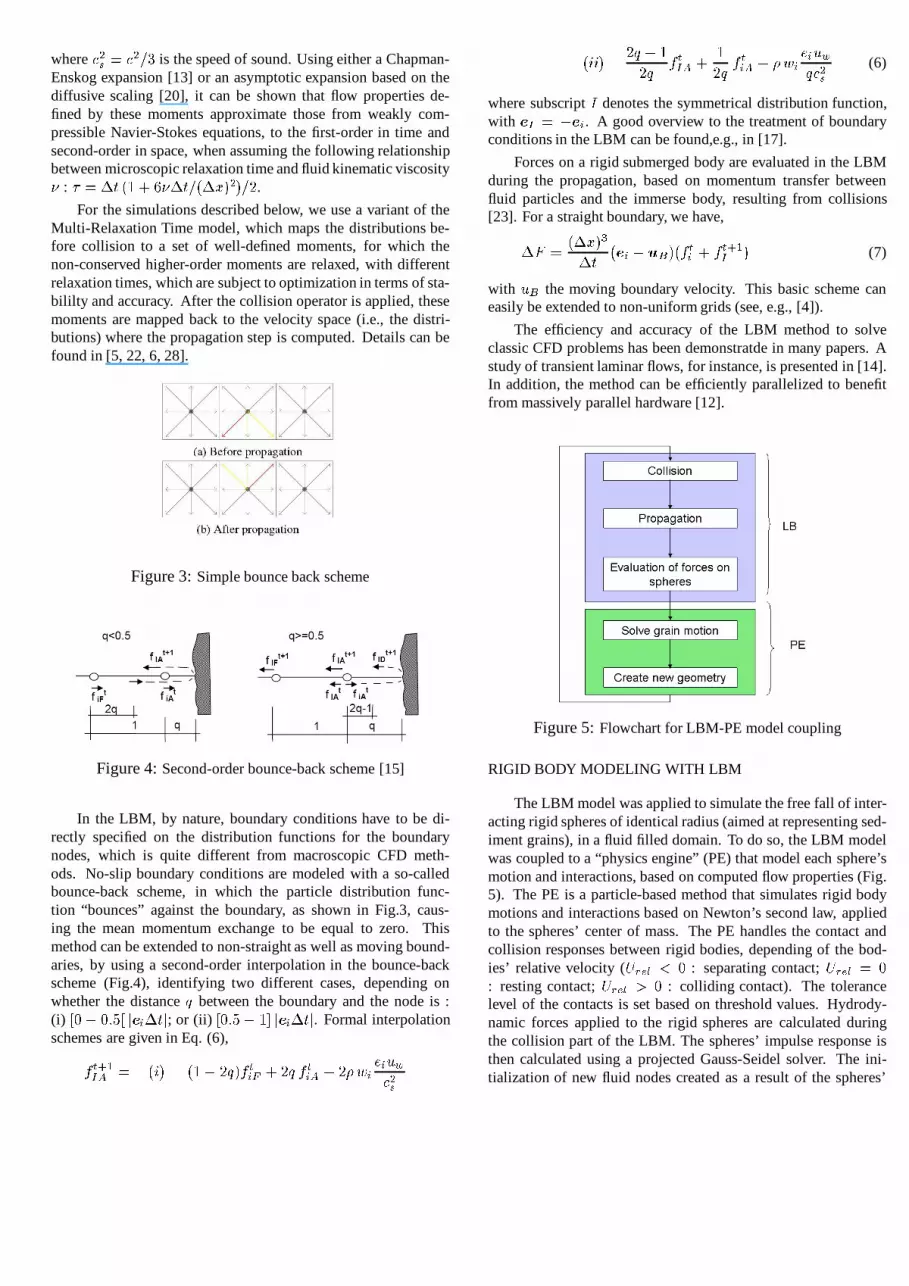
Figure 5:Flowchart for LBM-PE model coupling

RIGID BODY MODELING WITH LBM

The LBM model was applied to simulate the free fall of inter-acting rigid spheres of identical radius (aimed at representing sed-iment grains), in a fluid filled domain. To do so, the LBM modelwas coupled to a “physics engine” (PE) that model each sphere’smotion and interactions, based on computed flow properties (Fig.5). The PE is a particle-based method that simulates rigid bodymotions and interactions based on Newton’s second law, appliedto the spheres’ center of mass. The PE handles the contact andcollision responses between rigid bodies, depending of thebod-ies’ relative velocity (� � � �

�: separating contact;� � �

� �: resting contact;� � �

� �: colliding contact). The tolerance

level of the contacts is set based on threshold values. Hydrody-namic forces applied to the rigid spheres are calculated duringthe collision part of the LBM. The spheres’ impulse responseisthen calculated using a projected Gauss-Seidel solver. Theini-tialization of new fluid nodes created as a result of the spheres’

displacement is done by performing local collision/propagationsteps, on the newly created fluid nodes, until convergence ofthefluid characteristics (pressure/higher order moment) is achieved.This approach has helped improving the forces’ accuracy andre-ducing errors on both sphere drag force and velocity, as wellasoscillations of various parameters during the simulations.

Practically, the PE consists in a library of C++ routines,developed at the University of Erlangen-Nurnberg (Germany)[11], that is coupled to the LBM model for computing spheres’interactions and resulting changes in flow properties, in themanner described above. The simulation of free falling spheres issplit into two phases: (i) an initialization, in which each sphereis fixed to an initial position and the LBM model is run untilconvergence of flow properties to a steady state is achieved;(ii)each sphere is released to fall and interact with other spheres inthe cylinder, under the action of gravity.

APPLICATIONS OF LBM-PE MODEL

Flow in a circular pipe

We simulate a gravity driven laminar flow, through a slop-ing circular pipe of radius� and angle� , by specifying volumeforces :� # � � � � $ � � � � � in the LBM. For laminar flows, Navier-Stokes equations yield the classical axisymmetricPoiseuille flowsolution,

� � � � � � �� � #� � (8)

with � $ � the fluid dynamic viscosity.

The model is first run for a pipe of radius� � � � � m, slope

angle � � � , and length� � � � �

m, with a fluid of density$ � � � � � �kg/m� and kinematic viscosity� � � � � � �

m�/s. The

Reynolds numberRe=� � � � � � � � � � �

(with � � � � � � � � �m/s for

� � �from Eq. (8)) is well wihin the laminar regime.

Results are calculated for a series of increasingly refined LBMgrids sizes,

� � � � � � �to

� � � � �, starting from a state of rest;

in each case, time step is selected based on a CFL = 1 criterion.Periodic boundary conditions are specified at the inlet and outletboundaries (i.e., fields on the inlet boundary are set equal to thoseon the outlet boundary at the previous time step) and a no-slipboundary condition is applied at the wall (second-order bounce-back scheme). Table 1 shows relative mean, maximum, and RMSerrors of LBM results for the axial velocity� � � at the middlesection of the pipe, compared to the theoretical value from Eq. (8),as a function of grid size. We see that numerical results convergeto the analytic solution as grid size is reduced. A closer inspectionwould show that the convergence rate is� � � � � �

, as expectedfrom the selected LBM scheme.

The model is then run for higher slope angles, and thusReynolds numbers, in order to verify that numerical errors remainacceptable. Mean, maximum, and RMS errors are similarlyreported in Table 2, for the coarser grid size

� � � � � � �. We

see that numerical errors remain quite similar over a large rangeof Reynolds numbers within the laminar regime,Re � 1–21.

� �max. error RMS error mean error

5 � � � �

2.879 3.764 0.8642.5

� � � �1.452 1.483 0.237

1.66 � � � �

0.997 0.786 0.1021.25

� � � �0.754 0.556 0.063

1 � � � �

0.560 0.269 0.027

Table 1:Relative errors (%) of axial velocity� � � , compared toEq. (8), as a function of LBM grid size forRe = 1.07.

� Re max. error RMS error mean error

1 1.07 0.560 0.270 0.02710 10.65 0.523 0.258 0.02620 20.97 0.523 0.256 0.026

Table 2:Relative errors (%) of axial velocity� � � , compared toEq. (8), as a function of Reynolds number for

� � � � � � �.

Single falling sphere in a fluid

Assuming a sphere of radius� and density$ & , falling inan unbounded Newtonian fluid of density$ � and viscosity

,

the balance of weight (� � � � � � � � � � $ & � ) buoyancy (� �� � � � � � � � $ � � ) and drag (� � � � � � � $ � � � � � � � �

) forces (� �� � � ) yields a terminal velocity of,

� � � � �� � � � � � � � � � � � �

(9)

with � � $ & � $ � . AssumingRe� � � � � � � � �

(1) for laminarflows, Stokes solution yields the drag coefficent for the sphere :� � � � � �

Re.

Schiller and Naumann [25] extended the latter equation tohigherRe values as,� � � � � � � � � �

Re ! " # $ � �Re. Moreover,

for a finite width LBM domain, e.g., represented by a circularpipeof radius� , such as used in the above application, additional cor-rections must be made to� � values. These were given in [10] asa perturbation expansion of% � � � � , yielding,

� � & � � �Re

� � � Re� ! " # $ �

� � � � � � % '� � � � � � % � � � � � % � � � � � � � % ' � � � � � � � % " � (10)

which predicts the drag force� & � � � � � � $ � � � & � � � � �with a

95% accuracy, for% �� �

andRe � �

.

We run the LBM model for :� � � � m, � � � � �

m,$ & � � � � � �kg/m� , � � � � � �

m�/s and$ � � � � � � �

kg/m� ;length � � � �

m was selected in order for the sphere to reachsteady state before impacting the cylinder’s bottom. No-slipconditions are specified on the lateral boundary as well as onthetop and bottom sides of the cylinder, as recommended in [23].Avelocity continuity boundary condition is specified on the rigidsphere’s boundary (modified second-order bounce-back scheme

� �Error on� � & Error on �

0.0025 0.07 16.690.0017 0.08 9.160.0013 0.15 7.900.001 0.06 8.88

Table 3: Relative error (%) of computed drag coefficient� � &and fall velocity of the sphere� , as compared to theory (Eqs. (9)and (10)) for different grid sizes andRe=0.41.

$ & Re Error on� � & Error on �2,000 0.41 0.06 8.884,000 1.15 0.02 10.696,000 1.83 0.01 11.048,000 2.47 0.06 10.6610,000 3.09 0.29 9.84

Table 4:Same errors as in Table 3, for differentRe values, with� � � � � � �.

for moving boundaries, defined in [23]). We first performedcomputations in a series of increasingly refined LBM grids, withsize

� � � � � � � to 0.001, starting from a state of rest. As

before, time step is selected based on a CFL = 1 criterion. Table 3shows numerical errors for� � & and � as compared to Eqs. (9)and (10), for a lowRe=0.41, as a function of mesh size. We see areasonable convergence of numerical results towards the expectedvalues. We then use

� � � � � � �to compute the drag coefficient

and fall velocity as a function ofRe (changed by varying thesphere density). Table 4 shows a good accuracy for all selectedcases.

Figure 6: Simulation of 6 falling spheres (color scale indicatesvelocity magnitude) ; (a)-(d) shows results for increasingtime.

Multiple-spheres test-cases

Having validated LBM simulations for both a Poiseuilleflow and for one single falling/settling sphere, other caseswereperformed for multiple interacting falling spheres, for which notheoretical solution exists. Fig. 6 thus shows 4 stages of flow

Figure 7:LBM-PE simulations with 4,500 spheres in a cylindri-cal domain, for a specified inlet velocity achievingRe = 0.1; in(a)-(b), color reflect a pressure scale

and interactions of 6 falling spheres. Steady state is reached inFig. 6b and, in Fig. 6c, the 3 leading spheres are approachingthebottom and slow down. Hence, flow velocities increase ahead ofthe 3 following spheres. In Fig. 6d, spheres impact the cylinderbottom, rebound, and roll over each other.

Perspectives

More complex applications, which are still ongoing, will ul-timately involve the computation of unsteady flows in a circular(or rectangular) domain filled with a large number� (typically10,000) of interacting spheres of varying radii� , achieving aspecified porosity� , e.g., representing a porous medium in a mini-channel. For a cylindrical domain (� � � � , for instance, we find,

� � � � �� � � �

�% � � � � (11)

Similar to the work in [32], we are first testing cases of asteady flow through a sphere-filled pipe (e.g., Fig. 7), to verifythe standard Darcy law is retrieved for low porosity� . We willthen test cases with cyclic pressure loading at the pipe extremitiesand/or harmonic horizontal acceleration specified as a volumeforce. Such cases will yield soil liquefaction under some specificloading.

MICROFLUIDICS EXPERIMENTS

Experiments were performed in custom fabricated mini-channels (Fig. 1) filled with water, or with a mixture of waterand idealized sediment made of standardized glass beads of 10-50

m in diameter, to both provide data for LBM-PE model val-

idation and gain physical insight into the pore pressure responseof soils, due to dynamic seismic-like loading. Two different typesof experiments were designed and performed, for which pressurevariation was measured at several gates (side channels) along themain channel, using pressure transducers connected to a mani-fold (Fig. 1) : (a) steady state flows were created by specifying aconstant pressure gradient between both extremitites of the mini-channel; and (b) dynamic (essentially cyclic) pressure pulses weregenerated in the mini-channel using a pump.

We only tested one channel geometry so far, but we are plan-ning in future work to vary properties of the channel (cross-section/length/branches), together with the frequency and ampli-tude of the pressure variation, in order to investigate effects of

these on measurements, in relation to pore pressure generation insoils.

In all experiments, we first use pure water and estimateeffects of the channel itself on fluid flow, essentially throughenergy dissipation; this yields hydrodynamic characteristics of thechannel (e.g., friciton coefficient). We then repeat experimentsusing the mixture of water and glass beads and estimate thehydrodynamic properties of glass beads by removing the knownchannel effects. Cyclic test results will be processed thisway andwe will then attempt to correlate these to triaxial test results [16]and CFD simulations of both with the LBM-PE model.

Mini-channel and its equipment

Considerable efforts in miniaturization since the 1980s led tothe development of Micro Electro Mechanical Systems (MEMS),such as mini- and micro-channels, and to their increasing usein chemichal and biomedical applications. Here, we built mini-channels by soft-lithography, which allows for a quick fabricationof rectangular mini-channels, using the properties of polymeriza-tion of polydimethylsiloxane (PDMS).

The mini-channel shown in Fig. 1, used in experimentsreported here, is� � �

mm long, 1 mm wide, and 0.2 mm deep.Four branches, spaced 10 mm apart, allow for pressure measure-ments using transducers connected to 4 gates; 2 additional gatesare located at the entrance and exit of the main channel. These sixgates are connected to pressure transducers via a custom mademanifold (Fig. 1) The transducers are Honywell type stainlesssteel strain gauges (non-linearity of +/- 0.1% of the full scale,pressure range : 0–200 psi), and Omega DP25-S strain gaugepanel meters are used to digitize the pressure (Fig. 1); these areconnected to a control unit recording measurements at a specifiedsampling frequency (typically 12 Hz). A pressure panel (Fig. 1)is used to specify a constant or cyclic pressure at the channel inlet.

Experiments

Eq. (8) gives the axial flow velocity� � � � , in a circular cylin-der of radius� , due to a specified pressure gradient, for steadylaminar flows with lowRe (Poiseuille flow). The latter is typicalin microfluidics applications dominated by viscosity. Eq. (8) canstill be used as a reference for non-circular channels by introduc-ing the hydraulic diameter,� � � � � � �

, where�

is the chan-nel cross-sectional area and

�its perimeter. We further define:

Re� � � � � � , with � � � � �

the mean flow velocity, where�

denotes flow rate. With these definitions, Eq. (8) yields,

� � � � � � � � � � �� �� � with � � � �

�#� � � ��� � (12)

and� � � � � � �for a circular cross section. For Fig. 1’s channel

:� � � �

mm�,� � � �

mm and� � � � � � �mm.

In fluid flows through narrow pipes, changes in pressure takeplace along the length of the pipe, due to both continuous anddis-crete frictional losses. The former are due to viscous shearstressalong the pipe boundary, as in Eq. (12), while the latter are addi-tional energy losses due to abrupt changes in the pipe geometry,such as branching-out/inlet/outlet. Hence, the specified pressure

Figure 8: Pressure measured as a function of mean flow speed,in Fig. 1’s channel, filled with a water-bead mixture, at gate: G1(inlet) (� ); G2 (� ); G3 (� ); G4 ( ); G5 ( ). Solid lines denotequadratic curve fits forced to (0,0);# � �

(atmosph.) at gate G6.

gradient,

�# � � � � � # � � # � � � � , must overcome all such pressure

drops (i.e., head losses) due to energy losses, with# � the pressureat the inlet and# � at the outlet. If the mini-channel cross-sectionremains constant, for a constant flow rate, there is no changeinmean flow velocity along the pipe. Bernouilli equation can thenbe used to relate the total energy loss along the channel to thespecified pressure difference,

� # � # � � # � . Assuming a hori-zontal channel, we find,

� # � �� $ � � � � �� � � %

� (13)

with � � the average (continuous) skin friction coefficient and the � -th discrete head loss coefficient.

In mini-channel experiments with steady flows (Fig. 1), Eq.(13) can be applied between each pair of pressure gates. Thus, us-ing measured pressures, values of� � and are first calculated asa function of� (or more specifically as a funcion ofRe). Resultsare first calculated for pure water and then for the water-beadsmixture. The channel frictional properties can thus be removed toestimate those of the idealized saturated porous medium modeledby the glass beads, under various types of flows.

According to Darcy’s law, in a porous medium of low per-meability � (i.e., clays, silts), the small flow velocity is propor-tional to the pressure gradient:

� # � � $ � � � � � � ; this applieswhen Re �

�,000 or so. For larger permeability andRe val-

ues, according to Vorchheimer equation, a quadratic term appears:

� # � � $ � � � � � � � � � �; this applies whenRe

� � �,000 or so.

Eq. (10) is consistent with Darcy’s law prediction, since for smallRe : � � � � � � 1/Re � � � � ; hence, Eq. (13) yields

� # � �for the continuous friction term. By contrast, for largeRe, thedrag coefficient of a small rigid sphere becomes constant in theturbulent regime and Eq. (13) yields

� # � � �for the continuous

friction term, which is consistent with Vorchheimer equation.

Fig. 8 shows the pressure# measured at gates G1-G5 as afunction of mean flow speed� , in the mini-channel of Fig. 1 filled

Figure 9:Pressure drop between inlet and outlet, as a function offlow speed, in Fig. 1’s channel filled with a water-bead mixture :measurements (� ); linear (—–) and quadratic (- - - -) fits.

with a water-beads mixture. G1 denotes the inlet, and pressure atthe outlet G6 is atmospheric,# " � �

. Hence, in this configuration,� # � # � � # " . We see, pressure varies linearly for low� (�� � � �m/s) and then becomes quadratic. Specificaly, Fig. 9 plots� # as a function of� and shows both linear and quadratic fits,

representative of Darcy’s and Vorchheimer’s laws, respectively.With the former, we find� � � � � � � � ' m/s (� � � � � � �

), andwith the latter� � � � � � � � � ' m/s (� � � � � � �

). For � � � � � �m/s, the maximum observed value of the mean velocity, we haveRe = 1, indicating laminar creeping flows in all cases.

Similar experiments, run with the mini-channel filled onlywith water showed, as expected, much larger velocities, varyingbetween� � �

and 2 m/s for the same pressure gradients as inFig. 8. Eq. (13) was applied to those measurements and frictionalcharacteristics of the mini-channel,� � � and � � � � � � �

,were calculated. For the continuous friction coefficient wefound,in particular, � � � � � � � �

Re� � ! " �

(with � � � �). A similar

analysis was repeated for the results of Fig. 8 obtained for themini-channel filled with the water-bead mixture. We thus found,� � � � � � � � � �

� � � � � � �Re

� � ! � �(with � � � � � � �

), yieldingthe continuous friction coeficient due only to the water-beadmedium as, � � �

� � � � � Re

� � ! � # , which is close to thetheoretical value expected from Darcy’s law. Additionally, thediscontinuous coefficients for the water-bead filled channelwere obtained (not shown). These results, together with variousforms of Eq. (13), make it possible to predict the pressure atgates G1-G6, without running experiments, including variouscontributions to the pressure drop, Fig. 10, for instance showssuch a prediction for� � � � � � �

m/s.

CONCLUSIONS

Although computations described in the perspective sectionare sill ongoing and no comparison with microfluidics results weredone so far, based on prelminary results, we believe our LBM-PE approach is more general, consistent, and accurate than ear-lier proposed methods, and will yield a numerical tool able to

Figure 10:Pressure at gages G1-G6, for� � � � � � � m/s, in

Fig. 1’s channel filled with water-bead mixture : predicted con-tinuous losses in channel (� � � ) (� ); predicted continuous lossesdue to beads (� � � ) ( ); total predicted continuous losses (� � )(� ); predicted discrete losses due to branching ( ) ( ); totalpredicted losses (� ); total measured losses (- - - -).

investigate the micro-mechanical behavior of soilds undercom-plex seismically induced harmonic pore pressures and horizontalaccelerations.

Initial experiments performed in mini-channels filled withan idealized sediment, for steady flows, led to promising re-sults showing the expected fluid behaviors at the of the micro-mechanical level. Experiments with cyclic pressure loading areongoing and will be similarly analyzed in order to relate macro-scopic measured parameters, such as pressure drop, to the micro-mechanical properties of the medium. These experiments willboth help gaining additional physical insight into pore-pressurebuild-up and serve as a data set for validating the LBM-PE model,which in turn wil be use to perform broader parametric studies.

Ultimately, all these results will contribute to developing newmacroscopic constitutive laws for predicting underwater slidetriggering.

ACKNOWLEDGEMENTS

This research was supported by the NSF-PIRE program at URIand the TUB. The author would like to thank Klaus Iglberger(University of Nurnberg-Erlangen).

REFERENCE

[1] Abadie, S., Morichon, D., Grilli, S.T. and Glockner, S.(2008) “VOF/Navier-Stokes numerical modeling of sur-face waves generated by subaerial landslides,”La HouilleBlanche, 1 (Feb. 2008), 21-26.

[2] Ahrenholz, B., Tolke, J. and Krafczyk, M. (2006) ”Lattice-Boltzmann simulations in reconstructed parametrizedporous media,”Intl. J. Comp. Fluid Dyn., 20(6), 369-377.

[3] Bhatnagar, P.L., E.P. Gross and M. Krook (1954) “A Modelfor Collision Processes in Gases,”Phys. Rev., 94, 511-.

[4] Crouse, B., E. Rank, M. Krafczyk and J. Tolke (2002) “ALB-based approach for adaptive flow simulations,”J. Mod-ern Phys B, 17, 109-112.

[5] d’Humieres, D. (1992) “Generalized lattice-Boltzmannequations,”Rarefied Gas Dynamics: Theory and Simula-tions(Prog. Astronaut. Aeronaut., B. D. Shizgal and D. P.Weave, eds.), AIAA, Washington DC, Vol.159, 450–458.

[6] d’Humieres, D., Ginzburg, I., Krafczyk, M., Lallemand,P., and Luo, L. (2002) ”Multiple-relaxation-time latticeBoltzmann models in three dimensions,”Phil. Trans. R.Soc. Lond., A360, 437-451.

[7] Drouin Y. (2006)Study of soil liquefaction and its effectson tsunamogenics landslides.Senior Thesis Report, EcoleCentrale de Nantes/University of Rhode Island. 69 pps.

[8] Enet F. and Grilli S.T. (2005) ”Tsunami Landslide Gener-ation: Modelling and Experiments,”In Proc. 5th Intl. onOcean Wave Measurement and Analysis(Madrid, Spain,July 2005), IAHR Publ., paper 88, 10 pps.

[9] Enet, F. and Grilli, S.T. (2007) ”Experimental Study ofTsunami Generation by Three-dimensional Rigid Under-water Landslides,”J. Waterway Port Coast. and Oc. En-gng., 133(6), 442-454.

[10] Fayon, A., Happel, J. (1960) ”Effect of a cylindricalboundary on fixed rigid sphere in a moving fluid,”AIChEJ., 6(1), 55-58.

[11] Freudiger, S., J. Hegewald and M. Krafczyk (2008) “Sim-ulation of moving particles in 3D with the Lattice Boltz-mann method,”Comput. Math. with Appl., 55, 14611468.

[12] Freudiger, S., J. Hegewald and M. Krafczyk (2008) “A par-allelization concept for a multi-physics lattice Boltzmannprototypebased on hierarchical grids,”Intl. J. Comp. FluidDyn.(in press).

[13] Frisch, U., D. d’Humieres, B. Hasslacher, P. Lallemand,Y. Pomeau and J.-P. Rivet (1987) “Lattice Gas Hydrody-namics in Two and Three Dimensions,”J. Complex Syst.,1, 75–136.

[14] Geller, S., M. Krafczyk, J. Tolke, S. Turek and J.Hron (2006) “Benchmark computations based on Lattice-Boltzmann, Finite Element and Finite volume Methods forlaminar Flows,”Comp. and Fluids, 35, 888–897.

[15] Geller, S., J. Tolke and M. Krafczyk (2007)Lattice-Boltzmann Method on quadtree type grids for Fluid-Structure-Interaction, TU Braunschweig.

[16] Gemme, D.A. (2008)Effect of Particle Size on DynamicPore Pressure Buildup in Soils. Master’s Thesis, Dept. ofOcean Engng., Univ. of Rhode Island, 88 pps.

[17] Ginzburg, I. and D. d’Humieres (2003) “Multireflectionboundary conditions for lattice Boltzmann models,”Phys.Rev., 68, 606-614.

[18] Grilli, S.T., Ioualalen, M, Asavanant, J., Shi, F., Kirby, J.and Watts, P. (2007) ”Source Constraints and Model Sim-ulation of the December 26, 2004 Indian Ocean Tsunami,”J. Waterway Port Coast. and Oc. Engng., 133(6), 414-428.

[19] Grilli, S.T. and Watts, P. (2005) ”Tsunami generation bysubmarine mass failure Part I : Modeling, experimen-tal validation, and sensitivity analysis,”J. Waterway PortCoast. and Oc. Engng., 131(6), 283-297.

[20] Junk, M., A. Klar and L.-S. Luo (2005) “Asymptotic anal-ysis of the lattice Boltzmann equation,”J. Comp. Phys.,210(2), 676–704.

[21] Krafczyk, M., Lehmann, P., Philippova, O., Hnel, D. andLantermann, U. (2000) ”Lattice Boltzmann Simulations ofcomplex Multi-Phase Flows,Multifield Problems: State ofthe art”, Hrsg.: A.-M.-Sndig et al.,Springer Verlag, 50-57.

[22] Lallemand, P. and L.-S. Luo (2000) “Theory of the lat-tice Boltzmann method: Dispersion, dissipation, isotropy,Galilean invariance, and stability,”Phys. Rev., 61(6),6546–6562.

[23] Nguyen, N.Q., Ladd, A.J.C. (2004) ”Sedimentation ofhard-sphere suspensions at low Reynolds number,”J.Fluid Mech,535, 73-104.

[24] Qian, Y. H. , D. d’Humieres and P. Lallemand (1992) “Lat-tice BGK models for Navier-Stokes equation,”Europhys.Letters, 17(6), 479–484.

[25] Schiller, L., Naumann, A.Z. (1933) ”Uber die grundle-genden Berechnungen bei der Schwerkraftaufbereitung,”Zeitschrift Des Vereines Deutsc. Ing., 77(12), 318-320.

[26] Succi, S. (2001)The Lattice Boltzmann Equation for FluidDynamics and Beyond. Oxford University Press.

[27] Tappin, D.R., Watts, P. and Grilli, S.T. (2008) ”The PapuaNew Guinea tsunami of 1998: anatomy of a catastrophicevent,”Natural Haz. and Earth Syst. Sc., 8, 243-266.

[28] Tolke, J., S. Freudiger and M. Krafczyk (2006) “An adap-tive scheme for LBE multiphase flow simulations on hier-archical grids,”Comp. and Fluids, 35, 820-830.

[29] Tolke, J., Krafczyk, M., Schulz, M. and Rank, E. (2002)”Lattice Boltzmann simulations of binary flow throughporous media,”Phil. Trans. R. Soc. Lond., A360, 535-545.

[30] Watts, P., Grilli, S.T., Kirby, J. T., Fryer, G. J. and Tap-pin, D. R. (2003) ”Landslide tsunami case studies using aBoussinesq model and a fully nonlinear tsunami genera-tion model,”Natural Haz. and Earth Syst. Sc., 3, 391-402.

[31] Watts, P., Grilli, S.T., Tappin D., and Fryer, G.J. (2005)”Tsunami generation by submarine mass failure Part II :Predictive Equations and case studies,”J. Waterway PortCoast. and Oc. Engng., 131(6), 298-310.

[32] Zeghal, M. and El Shamy, U. (2004) “Dynamic responseand liquefaction of saturated granular soils: a micro-mechanical approach,”Cyclic Behaviour of Soils and Liq-uefaction Phenomena. Taylor & Francis Group, London.