A Model for Flow-enhanced Nucleation Based on Fibrillar Dormant Precursors

Full Paper

A Model for Flow-enhanced Nucleation Basedon Fibrillar Dormant Precursors

Peter C. Roozemond, Rudi J. A. Steenbakkers, Gerrit W. M. Peters*

A model for flow-enhanced nucleation is presented based on the concept of a polymer meltcontaining a fixed number of nucleation precursors with a fixed size distribution. Depending onthe size, precursors can either be active (i.e. susceptible to nucleation, the characteristic time scaleof which is governed by the deformation rate) andgrow into a spherulite or remain dormant. The sizedistribution of precursors is derived by combiningnucleation theory and experimentally determinedquiescent spherulite number densities. Longitudi-nal precursor growth, causing activation of dormantprecursors, is a function of molecular deformation:the stretch of high molecular weight chains. Boththe eXtended Pom-Pom and the Rolie-Poly modelare tested to calculate the molecular deformation.A quantitative agreement is found between simu-lations and experimental results.

Introduction

The mechanical properties of polymer products strongly

depend on processing conditions since these determine, to a

great extent, the structure. For semi-crystalline polymers,

flow-induced crystallization (FIC) plays a major role in this.

Crystallization of polymers can be divided into three

regimes;

(i) Q

P.MP.Fa

Macro

� 20

uiescent crystallization, if no flow is applied or the

flow is too weak to have a significant influence on the

crystallization process. Spherulitic crystalline struc-

tures (spherulites) are formed.

(ii) F
low-enhanced nucleation (FEN) occurs if the flow is
sufficiently strong (sufficiently high deformation rate

and time) to influence the nucleation kinetics. The

number density of spherulites is increased.

C. Roozemond, R. J. A. Steenbakkers, Gerrit W. M. Petersaterials Technology, Eindhoven University of Technology,O. Box 513, 5600MB, Eindhoven, The Netherlandsx: (þ31) 402447355; E-mail: [email protected]

mol. Theory Simul. 2011, 20, 000–000

11 WILEY-VCH Verlag GmbH & Co. KGaA, Weinheim wileyonlin

Early View Publication; these are NOT

(iii) O

elibrar

th

riented precursor structures are formed if a flow that

is sufficiently strong is applied for a longer period of

time. As a result, oriented crystalline structures, such

as shish-kebabs, are formed.

Different approaches are used to model FIC. Some

researchers start with the classical result for homogeneous

nucleation known as the Hoffman/Lauritzen expres-

sion.[1,2] It contains the free energy as a driving force of

which the entropic part is adapted by including the

decrease due to the molecular orientation caused by the

flow. A model using this approach was derived by Ziabicki

and Alfonso, but the entropy change due to orientation

alone could not reproduce effects as dramatic as observed

in experiments.[3] A second approach starts from the stat-

istical description of the evolution of the precursor size

distribution in the melt[4] and, again, incorporates the effect

of flow by adapting the free energy. For a model that

y.com DOI: 10.1002/mats.201000059 1

e final page numbers, use DOI for citation !! R

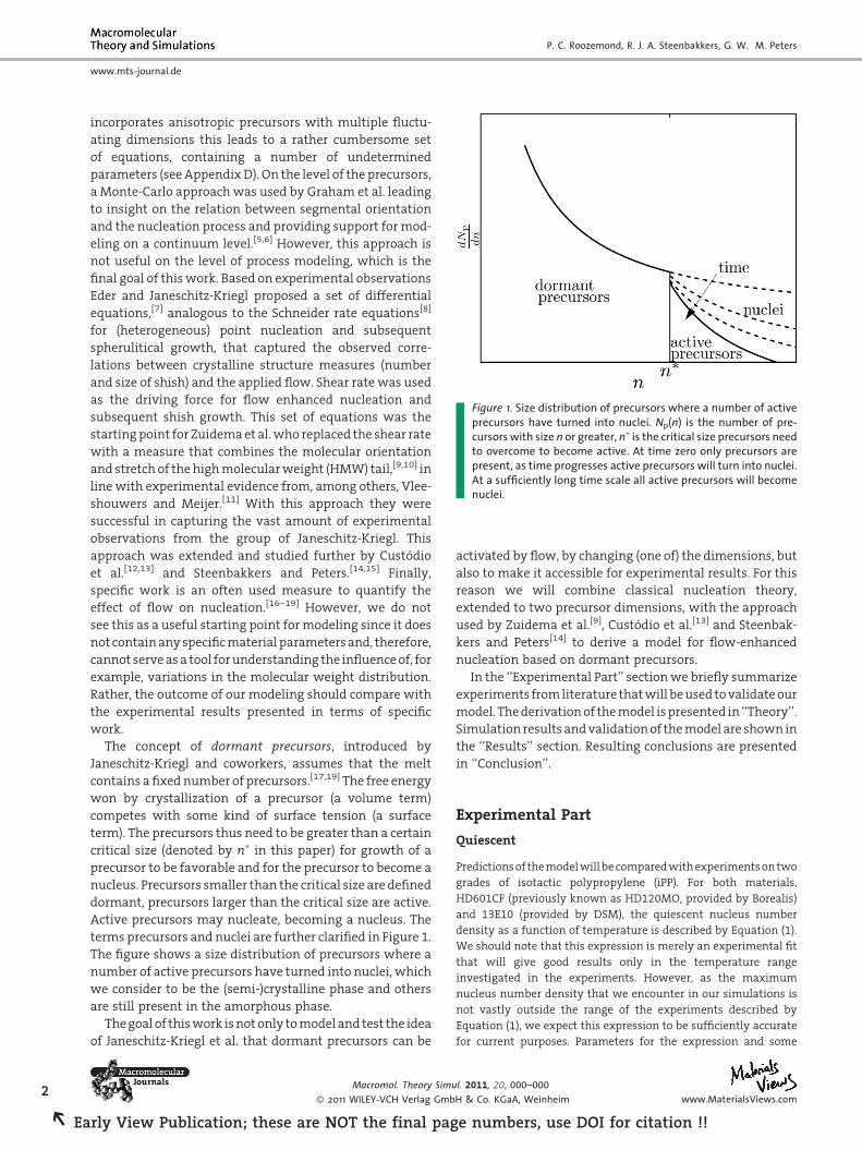
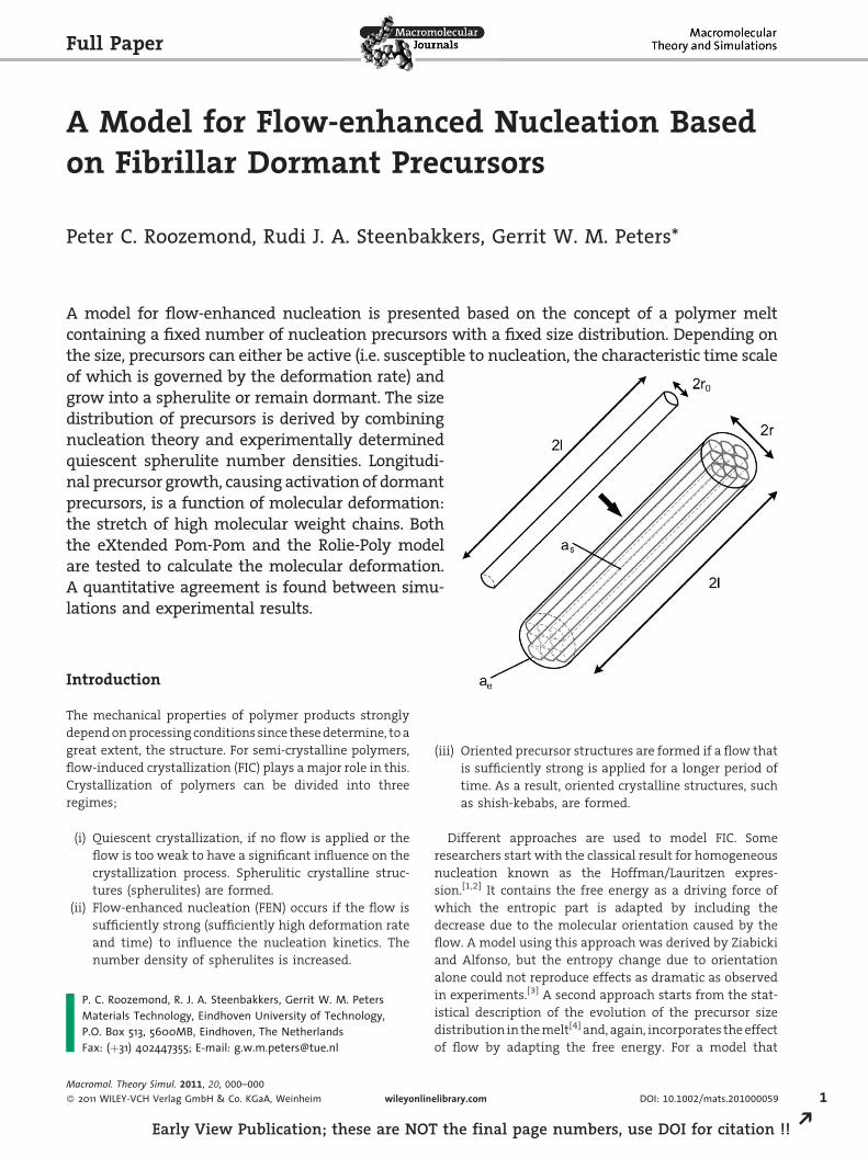
Figure 1. Size distribution of precursors where a number of activeprecursors have turned into nuclei. Np(n) is the number of pre-cursors with size n or greater, n� is the critical size precursors needto overcome to become active. At time zero only precursors arepresent, as time progresses active precursors will turn into nuclei.At a sufficiently long time scale all active precursors will becomenuclei.

2

REa

www.mts-journal.de

P. C. Roozemond, R. J. A. Steenbakkers, G. W. M. Peters

incorporates anisotropic precursors with multiple fluctu-

ating dimensions this leads to a rather cumbersome set

of equations, containing a number of undetermined

parameters (see Appendix D). On the level of the precursors,

a Monte-Carlo approach was used by Graham et al. leading

to insight on the relation between segmental orientation

and the nucleation process and providing support for mod-

eling on a continuum level.[5,6] However, this approach is

not useful on the level of process modeling, which is the

final goal of this work. Based on experimental observations

Eder and Janeschitz-Kriegl proposed a set of differential

equations,[7] analogous to the Schneider rate equations[8]

for (heterogeneous) point nucleation and subsequent

spherulitical growth, that captured the observed corre-

lations between crystalline structure measures (number

and size of shish) and the applied flow. Shear rate was used

as the driving force for flow enhanced nucleation and

subsequent shish growth. This set of equations was the

starting point for Zuidema et al. who replaced the shear rate

with a measure that combines the molecular orientation

and stretch of the high molecular weight (HMW) tail,[9,10] in

line with experimental evidence from, among others, Vlee-

shouwers and Meijer.[11] With this approach they were

successful in capturing the vast amount of experimental

observations from the group of Janeschitz-Kriegl. This

approach was extended and studied further by Custodio

et al.[12,13] and Steenbakkers and Peters.[14,15] Finally,

specific work is an often used measure to quantify the

effect of flow on nucleation.[16–19] However, we do not

see this as a useful starting point for modeling since it does

not contain any specific material parameters and, therefore,

cannot serve as a tool for understanding the influence of, for

example, variations in the molecular weight distribution.

Rather, the outcome of our modeling should compare with

the experimental results presented in terms of specific

work.

The concept of dormant precursors, introduced by

Janeschitz-Kriegl and coworkers, assumes that the melt

contains a fixed number of precursors.[17,19] The free energy

won by crystallization of a precursor (a volume term)

competes with some kind of surface tension (a surface

term). The precursors thus need to be greater than a certain

critical size (denoted by n� in this paper) for growth of a

precursor to be favorable and for the precursor to become a

nucleus. Precursors smaller than the critical size are defined

dormant, precursors larger than the critical size are active.

Active precursors may nucleate, becoming a nucleus. The

terms precursors and nuclei are further clarified in Figure 1.

The figure shows a size distribution of precursors where a

number of active precursors have turned into nuclei, which

we consider to be the (semi-)crystalline phase and others

are still present in the amorphous phase.

The goal of this work is not only to model and test the idea

of Janeschitz-Kriegl et al. that dormant precursors can be

Macromol. Theory Simu

� 2011 WILEY-VCH Verlag Gmb

rly View Publication; these are NOT the final pag

activated by flow, by changing (one of) the dimensions, but

also to make it accessible for experimental results. For this

reason we will combine classical nucleation theory,

extended to two precursor dimensions, with the approach

used by Zuidema et al.[9], Custodio et al.[13] and Steenbak-

kers and Peters[14] to derive a model for flow-enhanced

nucleation based on dormant precursors.

In the ‘‘Experimental Part’’ section we briefly summarize

experiments from literature that will be used to validate our

model. The derivation of the model is presented in ‘‘Theory’’.

Simulation results and validation of the model are shown in

the ‘‘Results’’ section. Resulting conclusions are presented

in ‘‘Conclusion’’.

Experimental Part

Quiescent

Predictions of the model will be compared with experiments on two

grades of isotactic polypropylene (iPP). For both materials,

HD601CF (previously known as HD120MO, provided by Borealis)

and 13E10 (provided by DSM), the quiescent nucleus number

density as a function of temperature is described by Equation (1).

We should note that this expression is merely an experimental fit

that will give good results only in the temperature range

investigated in the experiments. However, as the maximum

nucleus number density that we encounter in our simulations is

not vastly outside the range of the experiments described by

Equation (1), we expect this expression to be sufficiently accurate

for current purposes. Parameters for the expression and some

l. 2011, 20, 000–000

H & Co. KGaA, Weinheim www.MaterialsViews.com

e numbers, use DOI for citation !!

Table 1. Material parameters.

Material Grade Mw Mw=Mn Z¼Mw=Me Isotacticity Nref Tref TN Refs.

kg �mol�1 [-] [-] % m�3 -C -C�1

iPP2 HD601CF 365 5.4 70 97.5 1:14� 1013 110 0.115 [16,20]

iPP3 13E10 636 6.9 122 94.7 4:05� 1012 140 0.109 [16,21]

A Model for Flow-enhanced Nucleation Based on . . .

www.mts-journal.de

physical properties of the materials are shown in Table 1.

Numbering of the materials is adopted from Housmans et al.[16]

Figas

Figas

www.M

Nn ¼ Nref expð�cNðT�TrefÞÞ (1)

The above expression yields a cumulative number density

namely that of the nuclei obtained at constant temperature T in a

quiescent melt. Under these conditions, in temperature ranges of

practical interest, active precursors nucleate instantaneously, [17]

as evidenced by the narrow size distribution of spherulites even in

systems containing very low amounts of heterogeneous sub-

stances. Thus Nn is equal to the cumulative number of active

ure 2. Quiescent nucleus number density of iPP2 versus temperaturea function of shear time for different shear rates (b). Lines are to

ure 3. Quiescent nucleus number density of iPP3 versus temperaturea function of shear time for different shear rates (b). Lines are to

aterialsViews.com

Macromol. Theory Simul.



precursors per unit volume of the amorphous phase (their actual

number in general depends on the space filling at hand, which

depends on the thermal history). The differential number density

N0n,[19] which is obtained by calculating the increase in spherulite

number density DNn for a certain decrease of the temperature DT, or

(a) anguide

(a) anguide

2011, 2

H & Co

the

N0n ¼ �@Nn

@T¼ cNNref exp �cN T�Trefð Þð Þ (2)

From this expression the number of nuclei that will appear at a

certain temperature can be obtained by integration from the

experimental temperature to the nominal melting temperature.

Figure 2(a) and 3(a) show both the cumulative number density Nn

d flow-enhanced nucleus number density at T¼ 138 8C for iPP2,the eye.

d flow-enhanced nucleus number density at T¼ 138 8C for iPP3,the eye.

0, 000–000

. KGaA, Weinheim3

final page numbers, use DOI for citation !! R

2r0

2r2l

4

REa

www.mts-journal.de


and differential number density N0n for materials iPP2 and iPP3,

respectively. The solid line shows (1), the dashed line shows (2). The

circles show measurements of the spherulite number density

obtained from optical microscopy.[20,21]

2l

a s

a e

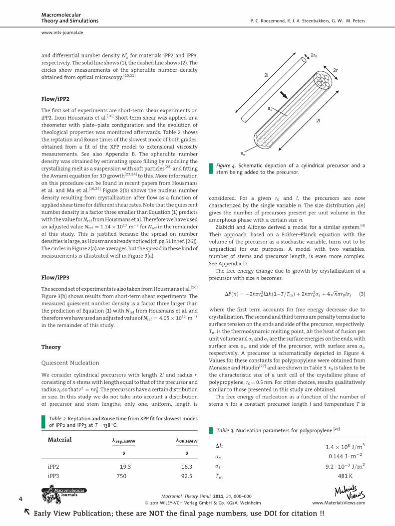
Figure 4. Schematic depiction of a cylindrical precursor and astem being added to the precursor.

Flow/iPP2

The first set of experiments are short-term shear experiments on

iPP2, from Housmans et al.[16] Short term shear was applied in a

rheometer with plate–plate configuration and the evolution of

rheological properties was monitored afterwards. Table 2 shows

the reptation and Rouse times of the slowest mode of both grades,

obtained from a fit of the XPP model to extensional viscosity

measurements. See also Appendix B. The spherulite number

density was obtained by estimating space filling by modeling the

crystallizing melt as a suspension with soft particles[22] and fitting

the Avrami equation for 3D growth[23,24] to this. More information

on this procedure can be found in recent papers from Housmans

et al. and Ma et al.[16,25] Figure 2(b) shows the nucleus number

density resulting from crystallization after flow as a function of

applied shear time for different shear rates. Note that the quiescent

number density is a factor three smaller than Equation (1) predicts

with the value for Nref from Housmans et al. Therefore we have used

an adjusted value Nref ¼ 1:14� 1013 m�3 for Nref in the remainder

of this study. This is justified because the spread on number

densities is large, as Housmans already noticed (cf. pg 51 in ref. [26]).

The circles in Figure 2(a) are averages, but the spread in these kind of

measurements is illustrated well in Figure 3(a).

Flow/iPP3

The second set of experiments is also taken from Housmans et al.[16]

Figure 3(b) shows results from short-term shear experiments. The

measured quiescent number density is a factor three larger than

the prediction of Equation (1) with Nref from Housmans et al. and

therefore we have used an adjusted value of Nref ¼ 4:05� 1012 m�3

in the remainder of this study.

Theory

Quiescent Nucleation

We consider cylindrical precursors with length 2l and radius r,

consisting of n stems with length equal to that of the precursor and

radius r0 so that r2 ¼ nr20. The precursors have a certain distribution

in size. In this study we do not take into account a distribution

of precursor and stem lengths; only one, uniform, length is

Table 2. Reptation and Rouse time from XPP fit for slowest modesof iPP2 and iPP3 at T¼ 138 8C.

Material lrep,HMW l0R,HMW

s s

iPP2 19.3 16.3

iPP3 750 92.5




considered. For a given r0 and l, the precursors are now

characterized by the single variable n. The size distribution r(n)

gives the number of precursors present per unit volume in the

amorphous phase with a certain size n.

Ziabicki and Alfonso derived a model for a similar system.[4]

Their approach, based on a Fokker–Planck equation with the

volume of the precursor as a stochastic variable, turns out to be

unpractical for our purposes. A model with two variables,

number of stems and precursor length, is even more complex.

See Appendix D.

The free energy change due to growth by crystallization of a

precursor with size n becomes

Tab

Dh

se

ss

Tm

l. 2011

H & Co

e nu

D~FðnÞ ¼ �2npr20lDh 1�T=Tmð Þ þ 2npr2

0se þ 4ffiffiffinp

pr0lss (3)

the first term accounts for free energy decrease due to
where
crystallization. The second and third terms are penalty terms due to

surface tension on the ends and side of the precursor, respectively.

Tm is the thermodynamic melting point, Dh the heat of fusion per

unit volume and se and ss are the surface energies on the ends, with

surface area ae, and side of the precursor, with surface area as,

respectively. A precursor is schematically depicted in Figure 4.

Values for these constants for polypropylene were obtained from

Monasse and Haudin[27] and are shown in Table 3. r0 is taken to be

the characteristic size of a unit cell of the crystalline phase of

polypropylene, r0¼ 0.5 nm. For other choices, results qualitatively

similar to those presented in this study are obtained.

The free energy of nucleation as a function of the number of

stems n for a constant precursor length l and temperature T is

le 3. Nucleation parameters for polypropylene.[27]

1:4� 108 J=m3

0.144 J �m�2

9:2 � 10�3 J=m2

481 K

, 20, 000–000

. KGaA, Weinheim www.MaterialsViews.com

mbers, use DOI for citation !!

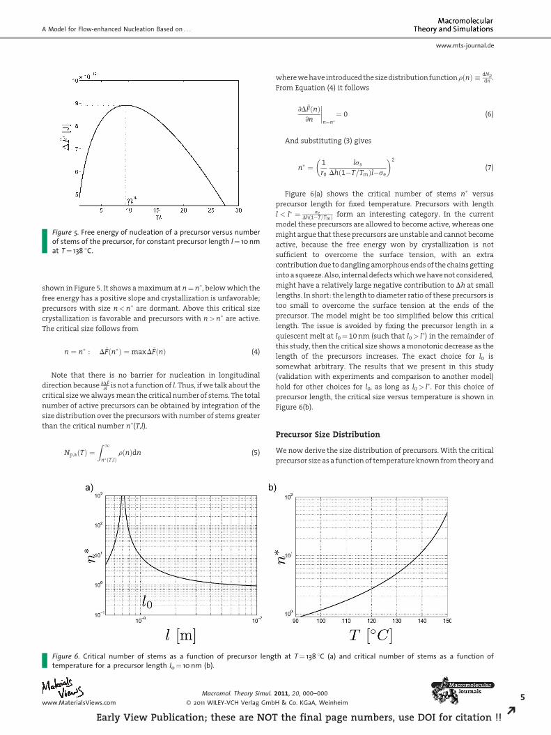
Figure 5. Free energy of nucleation of a precursor versus numberof stems of the precursor, for constant precursor length l¼ 10 nmat T¼ 138 8C.


www.mts-journal.de

shown in Figure 5. It shows a maximum at n¼n�, below which the

free energy has a positive slope and crystallization is unfavorable;

precursors with size n<n� are dormant. Above this critical size

crystallization is favorable and precursors with n>n� are active.

The critical size follows from

Figtem

www.M

n ¼ n� : D~Fðn�Þ ¼maxD~FðnÞ (4)

Note that there is no barrier for nucleation in longitudinal

direction because @D~F@l is not a function of l. Thus, if we talk about the

critical size we always mean the critical number of stems. The total

number of active precursors can be obtained by integration of the

size distribution over the precursors with number of stems greater

than the critical number n�(T,l),

Np;aðTÞ ¼Z 1

n�ðT;lÞrðnÞdn (5)

ure 6. Critical number of stems as a function of precursor lengperature for a precursor length l0¼ 10 nm (b).

aterialsViews.com




where we have introduced the size distribution functionrðnÞ � dNp

dn .

From Equation (4) it follows

th at T

2011, 2

H & Co

the

@D~FðnÞ@n

��n¼n�¼ 0 (6)

substituting (3) gives
And
n� ¼ 1

r0

lss

Dh 1�T=Tmð Þl�se

� �2

(7)

�
Figure 6(a) shows the critical number of stems n versus
precursor length for fixed temperature. Precursors with length

l < l� ¼ seDh 1�T=Tmð Þ form an interesting category. In the current

model these precursors are allowed to become active, whereas one

might argue that these precursors are unstable and cannot become

active, because the free energy won by crystallization is not

sufficient to overcome the surface tension, with an extra

contribution due to dangling amorphous ends of the chains getting

into a squeeze. Also, internal defects which we have not considered,

might have a relatively large negative contribution to Dh at small

lengths. In short: the length to diameter ratio of these precursors is

too small to overcome the surface tension at the ends of the

precursor. The model might be too simplified below this critical

length. The issue is avoided by fixing the precursor length in a

quiescent melt at l0¼10 nm (such that l0> l�) in the remainder of

this study, then the critical size shows a monotonic decrease as the

length of the precursors increases. The exact choice for l0 is

somewhat arbitrary. The results that we present in this study

(validation with experiments and comparison to another model)

hold for other choices for l0, as long as l0> l�. For this choice of

precursor length, the critical size versus temperature is shown in

Figure 6(b).

Precursor Size Distribution

We now derive the size distribution of precursors. With the critical

precursor size as a function of temperature known from theory and

¼ 138 8C (a) and critical number of stems as a function of

0, 000–000

. KGaA, Weinheim5

final page numbers, use DOI for citation !! R

6

REa

www.mts-journal.de


the differential nucleus number density at a range of temperatures

obtained from experiments, theory, and experiment can be

combined to obtain the number of precursors that become active

at a certain value for the critical size. Assuming, in accordance with

the idea of dormant precursors proposed by Janeschitz-Kriegl,[17,19]

that the size distribution is fixed, this gives us the precursor size

distribution. Using the expression for the differential number

density as a function of temperature Equation (2), and Equation (7)

for the critical size as a function of temperature, we obtain the

following expression for the size distribution as a function of

critical size r(n�)

d

dn�

Fig

rly V

Z 1n�ðTÞ

rðnÞdn ¼ NnðTÞ

Z 1n�ðTÞ

rðnÞdn ¼ �rðn�Þ ¼ @Nn

@T

@T

@n�

rðn�Þ ¼ cNNrefe�cN Tm 1�se=ðlDhÞ�ss=ðffiffiffiffin�p

r0DhÞð Þ�Trefð Þ

� ssTm

2Dhr0n�ffiffiffiffiffin�p

(8)

In our model the size distribution of precursors does not change

with temperature and thus the above equation is valid as a size

distribution function

rðnÞ ¼ cNNrefe�cN Tm 1�se=ðlDhÞ�ss=ðffiffiffinp

r0DhÞð Þ�Trefð Þ ssTm

2Dhr0n32

(9)

The size distribution of precursors in the melt calculated using

the above procedure for both iPP2 and iPP3 is shown in Figure 7.

Flow-enhanced Nucleation

The effect of flow is modeled by increasing the length of the

precursors by an amount of Dl. Precursors with length l that are

dormant in a quiescent melt (i.e., n<n�(l)) may become active

because, as shown in Figure 6(a), n� for a precursor with length

lþ Dl is smaller than the critical size for a precursor with length l; i.e.

ure 7. Size distribution of precursors for iPP2 and iPP3.



iew Publication; these are NOT the final pag

activation by flow occurs if n > n�ðlþ DlÞ, where n�ðlþ DlÞ is the

critical number of stems for a precursor with length lþ Dl.

The time evolution of the number of active precursors, i.e. the

number of precursors pushed over the activation barrier per unit

time, can be expressed in the following way

l. 2011

H & Co

e nu

_Np;a¼ �dNp;a

dn�_n��Np;a

tpn

¼ �rðn�Þ @n�

@l_lþ @n�

@T_T

� ��Np;a

tpn

(10)

where _l is the longitudinal precursor growth rate, the total length

increase follows from integration over time of the growth rate,

Dl ¼R

_ldt. The first term accounts for the number of precursors

activated by the flow per unit time. All simulations in this paper

are in isothermal conditions and thus _T ¼ 0, but the model can

also be used to simulate non isothermal cases. The second term

comes from active precursors nucleating, which happens with a

characteristic timescale tpn,

_Nn ¼Np;a

tpn(11)

well known that microscopic pictures of iPP during flow-
It is
enhanced nucleation experiments show that all spherulites

become visible at approximately the same moment in time, and

that their diameters are nearly equal.[15,28] This means that the

large majority of nuclei is created at approximately the same

moment in time. Furthermore, we have not observed significant

numbers of spherulites during flow in our current and previous

experimental work, even when the duration of flow was long

enough to observe them with optical microscopy.[14,15] This

assumption is supported by X-ray measurements of Mahendra-

singam et al. during film drawing of PET.[29] They observed that, for

high strain rates, crystallinity only started developing after the end

of the draw. Based on these observations, we assume that the

characteristic time of nucleation is much longer than the duration

of flow in our short-term shear experiments and that nucleation is

instantaneous in the absence of flow. Hence we set tpn¼1 during

flow and tpn¼0 after flow.

We notice that the precursor activation rate (Eq. 10) can be

written as a factor times the longitudinal growth rate _l for

isothermal flow-enhanced nucleation. This factor, �rðn�Þ @n�@l is

shown for a range of lengths in Figure 8. Because this quantity does

not vary largely (just a factor 4) over the range of precursors lengths

encountered in experiments (the maximum length reached is

�35 nm, see Figure 12(b)), the creation rate of active precursors (in

the absence of nucleation) is approximately proportional to the

growth rate of the precursors.

_Np;a � _l (12)

It is well known that the high molecular weight (HMW) fraction

of a polydisperse melt has a dominant influence on the flow-

enhanced nucleation process.[11,30–32] Steenbakkers and Peters

found the fourth power of the average stretch of the primitive

paths of chains in the HMW mode of the material (L) to be a good

measure of the increase in nucleation rate.[14,15] Graham and

, 20, 000–000



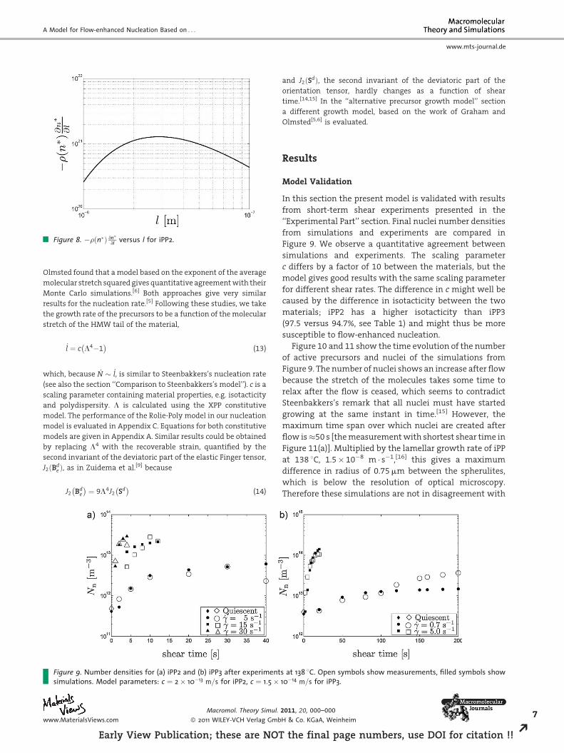
Figure 8. �rðn�Þ @n�@l versus l for iPP2.


www.mts-journal.de

Olmsted found that a model based on the exponent of the average

molecular stretch squared gives quantitative agreement with their

Monte Carlo simulations.[6] Both approaches give very similar

results for the nucleation rate.[5] Following these studies, we take

the growth rate of the precursors to be a function of the molecular

stretch of the HMW tail of the material,

Figsim

www.M

_l ¼ c L4�1� �

(13)

which, because _N � _l, is similar to Steenbakkers’s nucleation rate

(see also the section ‘‘Comparison to Steenbakkers’s model’’). c is a

scaling parameter containing material properties, e.g. isotacticity

and polydispersity. L is calculated using the XPP constitutive

model. The performance of the Rolie-Poly model in our nucleation

model is evaluated in Appendix C. Equations for both constitutive

models are given in Appendix A. Similar results could be obtained

by replacing L4 with the recoverable strain, quantified by the

second invariant of the deviatoric part of the elastic Finger tensor,

J2ðBde Þ, as in Zuidema et al.[9] because

J2 Bde

� �¼ 9L4J2 Sd

� �(14)

ure 9. Number densities for (a) iPP2 and (b) iPP3 after experimentulations. Model parameters: c ¼ 2� 10�13 m=s for iPP2, c ¼ 1:5�

aterialsViews.com




and J2ðSdÞ, the second invariant of the deviatoric part of the

orientation tensor, hardly changes as a function of shear

time.[14,15] In the ‘‘alternative precursor growth model’’ section

a different growth model, based on the work of Graham and

Olmsted[5,6] is evaluated.

Results

Model Validation

In this section the present model is validated with results

from short-term shear experiments presented in the

‘‘Experimental Part’’ section. Final nuclei number densities

from simulations and experiments are compared in

Figure 9. We observe a quantitative agreement between

simulations and experiments. The scaling parameter

c differs by a factor of 10 between the materials, but the

model gives good results with the same scaling parameter

for different shear rates. The difference in c might well be

caused by the difference in isotacticity between the two

materials; iPP2 has a higher isotacticity than iPP3

(97.5 versus 94.7%, see Table 1) and might thus be more

susceptible to flow-enhanced nucleation.

Figure 10 and 11 show the time evolution of the number

of active precursors and nuclei of the simulations from

Figure 9. The number of nuclei shows an increase after flow

because the stretch of the molecules takes some time to

relax after the flow is ceased, which seems to contradict

Steenbakkers’s remark that all nuclei must have started

growing at the same instant in time.[15] However, the

maximum time span over which nuclei are created after

flow is�50 s [the measurement with shortest shear time in

Figure 11(a)]. Multiplied by the lamellar growth rate of iPP

at 138 8C, 1.5� 10�8 m � s�1,[16] this gives a maximum

difference in radius of 0.75 mm between the spherulites,

which is below the resolution of optical microscopy.

Therefore these simulations are not in disagreement with

s at 138 8C. Open symbols show measurements, filled symbols show10�14 m=s for iPP3.

2011, 20, 000–000

H & Co. KGaA, Weinheim7

the final page numbers, use DOI for citation !! R

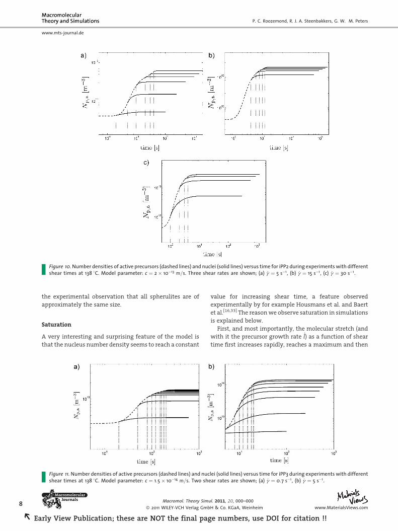
Figure 10. Number densities of active precursors (dashed lines) and nuclei (solid lines) versus time for iPP2 during experiments with differentshear times at 138 8C. Model parameter: c ¼ 2� 10�13 m=s. Three shear rates are shown; (a) _g ¼ 5 s�1, (b) _g ¼ 15 s�1, (c) _g ¼ 30 s�1.

8

REa

www.mts-journal.de


the experimental observation that all spherulites are of

approximately the same size.

Saturation

A very interesting and surprising feature of the model is

that the nucleus number density seems to reach a constant

Figure 11. Number densities of active precursors (dashed lines) and nucshear times at 138 8C. Model parameter: c ¼ 1:5� 10�14 m=s. Two she




value for increasing shear time, a feature observed

experimentally by for example Housmans et al. and Baert

et al.[16,33] The reason we observe saturation in simulations

is explained below.

First, and most importantly, the molecular stretch (and

with it the precursor growth rate _l) as a function of shear

time first increases rapidly, reaches a maximum and then

lei (solid lines) versus time for iPP3 during experiments with differentar rates are shown; (a) _g ¼ 0:7 s�1, (b) _g ¼ 5 s�1.

l. 2011, 20, 000–000



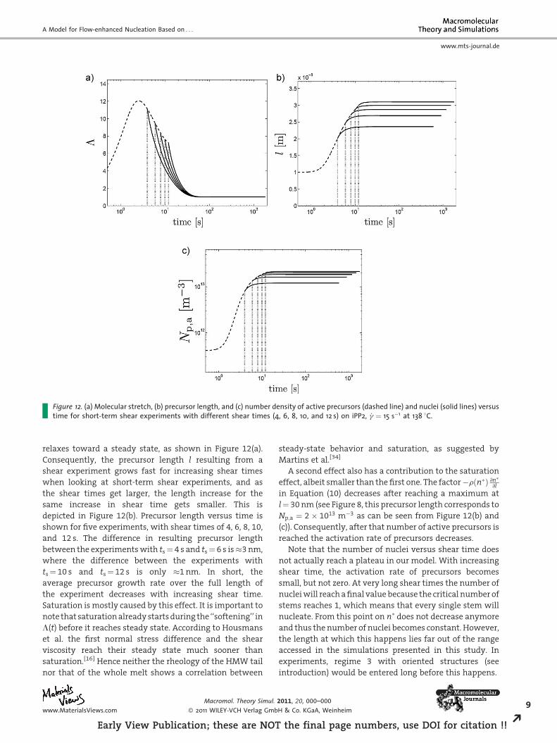
Figure 12. (a) Molecular stretch, (b) precursor length, and (c) number density of active precursors (dashed line) and nuclei (solid lines) versustime for short-term shear experiments with different shear times (4, 6, 8, 10, and 12 s) on iPP2, _g ¼ 15 s�1 at 138 8C.


www.mts-journal.de

relaxes toward a steady state, as shown in Figure 12(a).

Consequently, the precursor length l resulting from a

shear experiment grows fast for increasing shear times

when looking at short-term shear experiments, and as

the shear times get larger, the length increase for the

same increase in shear time gets smaller. This is

depicted in Figure 12(b). Precursor length versus time is

shown for five experiments, with shear times of 4, 6, 8, 10,

and 12 s. The difference in resulting precursor length

between the experiments with ts¼ 4 s and ts¼ 6 s is�3 nm,

where the difference between the experiments with

ts¼ 10 s and ts¼ 12 s is only �1 nm. In short, the

average precursor growth rate over the full length of

the experiment decreases with increasing shear time.

Saturation is mostly caused by this effect. It is important to

note that saturation already starts during the ‘‘softening’’ in

L(t) before it reaches steady state. According to Housmans

et al. the first normal stress difference and the shear

viscosity reach their steady state much sooner than

saturation.[16] Hence neither the rheology of the HMW tail

nor that of the whole melt shows a correlation between

www.MaterialsViews.com




steady-state behavior and saturation, as suggested by

Martins et al.[34]

A second effect also has a contribution to the saturation

effect, albeit smaller than the first one. The factor�rðn�Þ @n�@l

in Equation (10) decreases after reaching a maximum at

l¼ 30 nm (see Figure 8, this precursor length corresponds to

Np;a ¼ 2� 1013 m�3 as can be seen from Figure 12(b) and

(c)). Consequently, after that number of active precursors is

reached the activation rate of precursors decreases.

Note that the number of nuclei versus shear time does

not actually reach a plateau in our model. With increasing

shear time, the activation rate of precursors becomes

small, but not zero. At very long shear times the number of

nuclei will reach a final value because the critical number of

stems reaches 1, which means that every single stem will

nucleate. From this point on n� does not decrease anymore

and thus the number of nuclei becomes constant. However,

the length at which this happens lies far out of the range

accessed in the simulations presented in this study. In

experiments, regime 3 with oriented structures (see

introduction) would be entered long before this happens.

2011, 20, 000–000



10

REa

www.mts-journal.de


Comparison with Steenbakkers’s Model

We compare simulation results from our model with

the model presented by Steenbakkers and Peters.[14,15]

The flow-induced creation rate of active precursors in this

model can be simplified to

rly V

_Npf ¼ gp L4�1� �

�Npf

tpn(15)

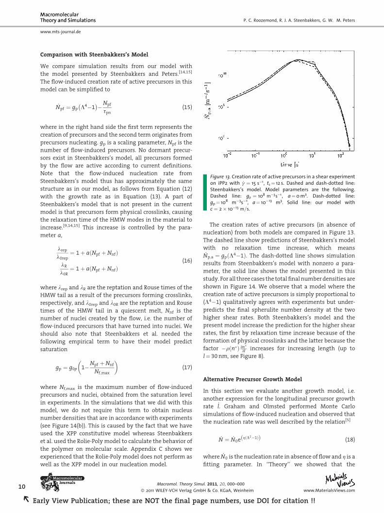
Figure 13. Creation rate of active precursors in a shear experimenton iPP2 with _g ¼ 15 s�1, ts¼ 12 s. Dashed and dash-dotted line:Steenbakkers’s model. Model parameters are the following.Dashed line: gp ¼ 108 m�3s�1, a¼0 m3. Dash-dotted line:gp¼ 108 m�3s�1, a¼ 10�13 m3. Solid line: our model withc ¼ 2� 10�13 m=s.

where in the right hand side the first term represents the

creation of precursors and the second term originates from

precursors nucleating. gp is a scaling parameter, Npf is the

number of flow-induced precursors. No dormant precur-

sors exist in Steenbakkers’s model, all precursors formed

by the flow are active according to current definitions.

Note that the flow-induced nucleation rate from

Steenbakkers’s model thus has approximately the same

structure as in our model, as follows from Equation (12)

with the growth rate as in Equation (13). A part of

Steenbakkers’s model that is not present in the current

model is that precursors form physical crosslinks, causing

the relaxation time of the HMW modes in the material to

increase.[9,14,15] This increase is controlled by the para-

meter a,

lrep

l0rep¼ 1þ aðNpf þ NnfÞ

lR

l0R¼ 1þ aðNpf þ NnfÞ

(16)

where lrep and lR are the reptation and Rouse times of the

HMW tail as a result of the precursors forming crosslinks,

respectively, and l0rep and l0R are the reptation and Rouse

times of the HMW tail in a quiescent melt, Nnf is the

number of nuclei created by the flow, i.e. the number of

flow-induced precursors that have turned into nuclei. We

should also note that Steenbakkers et al. needed the

following empirical term to have their model predict

saturation

gp ¼ g0p 1�Npf þ Nnf

Nf;max

� �(17)

where Nf,max is the maximum number of flow-induced

precursors and nuclei, obtained from the saturation level

in experiments. In the simulations that we did with this

model, we do not require this term to obtain nucleus

number densities that are in accordance with experiments

(see Figure 14(b)). This is caused by the fact that we have

used the XPP constitutive model whereas Steenbakkers

et al. used the Rolie-Poly model to calculate the behavior of

the polymer on molecular scale. Appendix C shows we

experienced that the Rolie-Poly model does not perform as

well as the XPP model in our nucleation model.




The creation rates of active precursors (in absence of

nucleation) from both models are compared in Figure 13.

The dashed line show predictions of Steenbakkers’s model

with no relaxation time increase, which means_Np;a ¼ gpðL4�1Þ. The dash-dotted line shows simulation

results from Steenbakkers’s model with nonzero a para-

meter, the solid line shows the model presented in this

study. For all three cases the total final number densities are

shown in Figure 14. We observe that a model where the

creation rate of active precursors is simply proportional to

(L4�1) qualitatively agrees with experiments but under-

predicts the final spherulite number density at the two

higher shear rates. Both Steenbakkers’s model and the

present model increase the prediction for the higher shear

rates, the first by relaxation time increase because of the

formation of physical crosslinks and the latter because the

factor �rðn�Þ @n�@l increases for increasing length (up to

l¼ 30 nm, see Figure 8).

Alternative Precursor Growth Model

In this section we evaluate another growth model, i.e.

another expression for the longitudinal precursor growth

rate _l. Graham and Olmsted performed Monte Carlo

simulations of flow-induced nucleation and observed that

the nucleation rate was well described by the relation[5]

l. 2011

H & Co

e nu

_N ¼ _N0e hðL2�1Þð Þ (18)

where _N0 is the nucleation rate in absence of flow and h is a

fitting parameter. In ‘‘Theory’’ we showed that the

, 20, 000–000



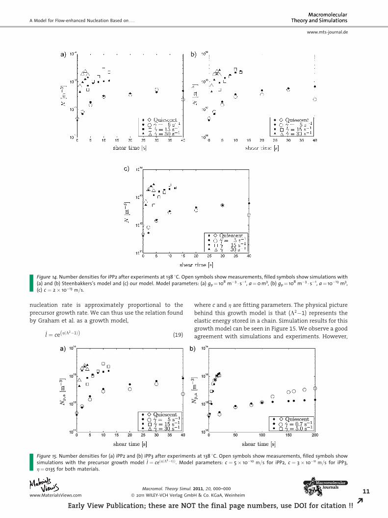
Figure 14. Number densities for iPP2 after experiments at 138 8C. Open symbols show measurements, filled symbols show simulations with(a) and (b) Steenbakkers’s model and (c) our model. Model parameters: (a) gp¼ 108 m�3 � s�1, a¼0 m3, (b) gp¼ 108 m�3 � s�1, a¼ 10�13 m3,(c) c ¼ 2� 10�13 m=s.


www.mts-journal.de

nucleation rate is approximately proportional to the

precursor growth rate. We can thus use the relation found

by Graham et al. as a growth model,

Figsimh¼

www.M

_l ¼ ce hðL2�1Þð Þ (19)

ure 15. Number densities for (a) iPP2 and (b) iPP3 after experimentulations with the precursor growth model _l ¼ ceðhðL

2�1ÞÞ. Model0135 for both materials.

aterialsViews.com




where c and h are fitting parameters. The physical picture

behind this growth model is that (L2�1) represents the

elastic energy stored in a chain. Simulation results for this

growth model can be seen in Figure 15. We observe a good

agreement with simulations and experiments. However,

s at 138 8C. Open symbols show measurements, filled symbols showparameters: c ¼ 5� 10�10 m=s for iPP2, c ¼ 3� 10�11 m=s for iPP3,

2011, 20, 000–000



12

REa

www.mts-journal.de


we prefer the power law of molecular stretch (Eq. 13)

because it requires just one scaling parameter to give

equally good results.

Conclusion

A model was derived for flow-enhanced nucleation based

on the concept of a melt containing a fixed number of

fibrillar flow-activatable nucleation precursors. Longitudi-

nal precursor growth, causing activation of dormant

precursors, is a function of molecular deformation: the

average stretch of the primitive path of chains in the HMW

tail of the material, calculated from a rheological consti-

tutive model. Both the Rolie-Poly and the eXtended Pom-

Pom model were evaluated. The nucleation model was

found to perform best in combination with the XPP model.

Simulations of the model give quantitative agreement with

experiments on two grades of iPP. Per material, a single

scaling parameter suffices for the whole range of shear rates

applied. The difference in scaling parameter between the

two grades can be explained by the different isotacticities of

the materials. Surprisingly, the model predicts saturation of

the number density of nuclei with increasing shear time

without any phenomenological terms. The model can also

be applied to non-isothermal cases.

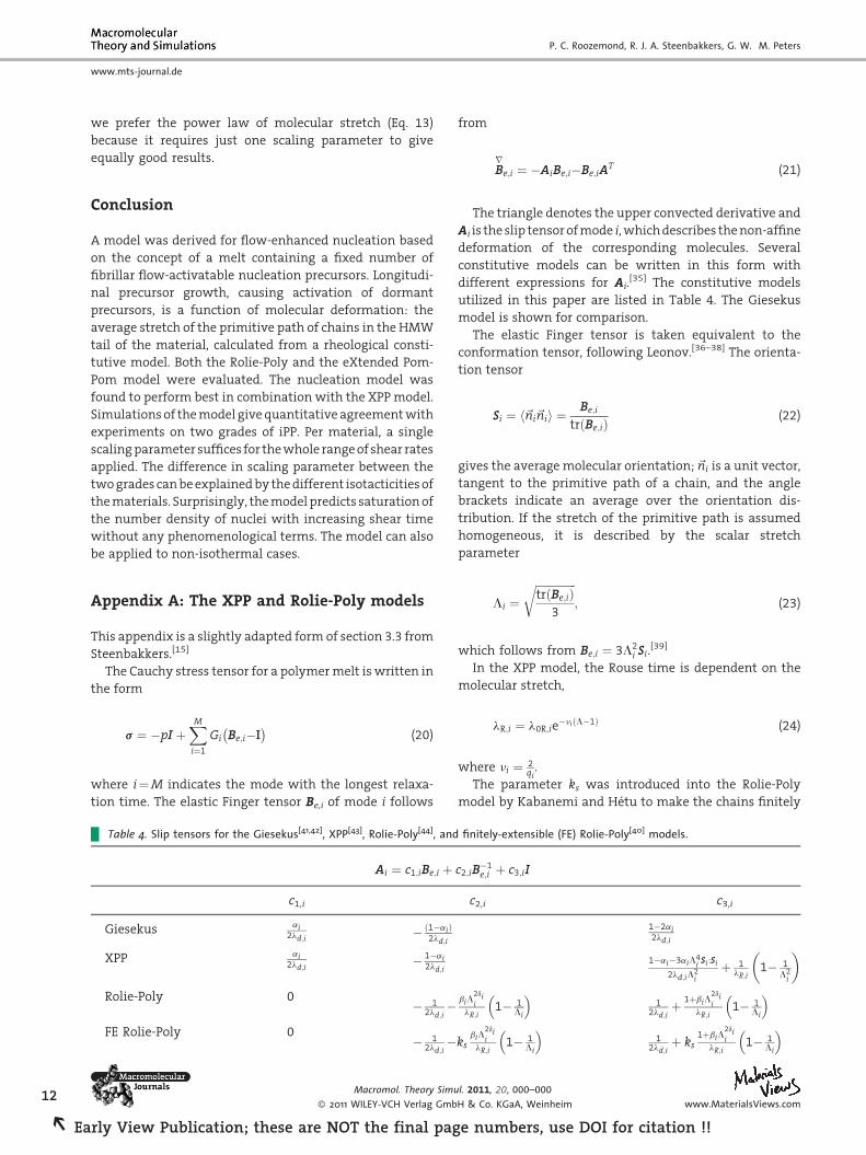
Appendix A: The XPP and Rolie-Poly models

This appendix is a slightly adapted form of section 3.3 from

Steenbakkers.[15]

The Cauchy stress tensor for a polymer melt is written in

the form

Tab

Gie

XPP

Rol

FE

rly V

s ¼ �pI þXM

i¼1

Gi Be;i�I� �

(20)

where i¼M indicates the mode with the longest relaxa-

tion time. The elastic Finger tensor Be,i of mode i follows

le 4. Slip tensors for the Giesekus[41,42], XPP[43], Rolie-Poly[44], and

Ai ¼ c1;iBe;i þ

c1,i

sekus ai2ld;i

� ð1�aiÞ2ld;i

ai2ld;i

� 1�ai2ld;i

ie-Poly 0� 1

2ld;i�

Rolie-Poly 0� 1

2ld;i�




from

finite

c2;iB�1e;i

c2,i

biL2dii

lR;i

�

ksbiL

2d

ilR;i

l. 2011

H & Co

e nu

Br

e;i ¼ �AiBe;i�Be;iAT (21)

The triangle denotes the upper convected derivative and

Ai is the slip tensor of mode i, which describes the non-affine

deformation of the corresponding molecules. Several

constitutive models can be written in this form with

different expressions for Ai.[35] The constitutive models

utilized in this paper are listed in Table 4. The Giesekus

model is shown for comparison.

The elastic Finger tensor is taken equivalent to the

conformation tensor, following Leonov.[36–38] The orienta-

tion tensor

Si ¼ h~ni~nii ¼Be;i

trðBe;iÞ(22)

gives the average molecular orientation; ~ni is a unit vector,

tangent to the primitive path of a chain, and the angle

brackets indicate an average over the orientation dis-

tribution. If the stretch of the primitive path is assumed

homogeneous, it is described by the scalar stretch

parameter

Li ¼ffiffiffiffiffiffiffiffiffiffiffiffiffiffiffitrðBe;iÞ

3

r; (23)

which follows from Be;i ¼ 3L2i Si.

[39]

In the XPP model, the Rouse time is dependent on the

molecular stretch,

lR;i ¼ l0R;ie�niðL�1Þ (24)

where ni ¼ 2qi

.

The parameter ks was introduced into the Rolie-Poly

model by Kabanemi and Hetu to make the chains finitely

ly-extensible (FE) Rolie-Poly[40] models.

þ c3;iI

c3,i

1�2ai2ld;i

1�ai�3aiL4i

Si :Si

2ld;iL2i

þ 1lR;i

1� 1L2

i

� �

1� 1Li

1

2ld;iþ 1þbiL

2dii

lR;i1� 1

Li

� i

1� 1Li

� 1

2ld;iþ ks

1þbiL2dii

lR;i1� 1

Li

�

, 20, 000–000




www.mts-journal.de

extensible.[40] ks is a nonlinear spring coefficient, given by

Figsho

www.M

ksðLÞ ¼1�1=L2

max

� �3�L2=L2

max

� �1�L2=L2

max

� �3�1=L2

max

� � (25)

where Lmax is the maximum molecular stretch possible.

Appendix B: Parameters for the ConstitutiveModels

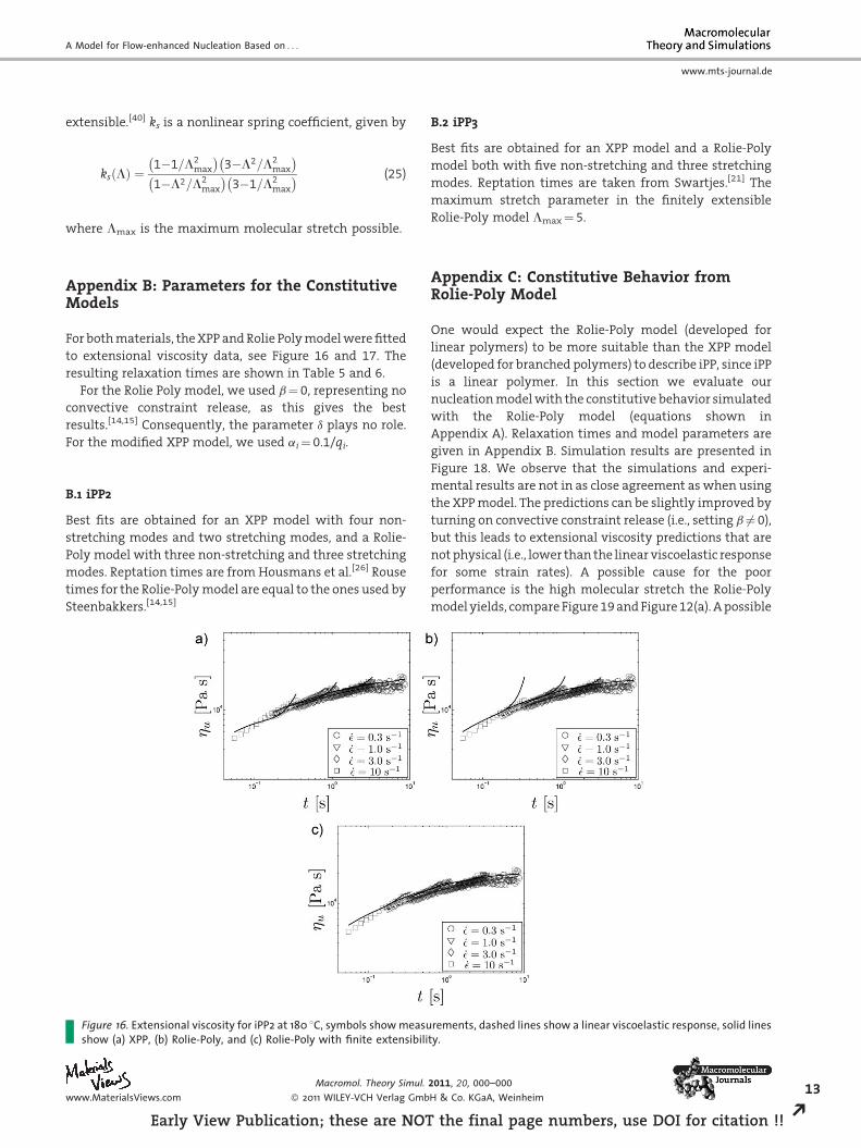
For both materials, the XPP and Rolie Poly model were fitted

to extensional viscosity data, see Figure 16 and 17. The

resulting relaxation times are shown in Table 5 and 6.

For the Rolie Poly model, we used b¼ 0, representing no

convective constraint release, as this gives the best

results.[14,15] Consequently, the parameter d plays no role.

For the modified XPP model, we used ai¼ 0.1/qi.

B.1 iPP2

Best fits are obtained for an XPP model with four non-

stretching modes and two stretching modes, and a Rolie-

Poly model with three non-stretching and three stretching

modes. Reptation times are from Housmans et al.[26] Rouse

times for the Rolie-Poly model are equal to the ones used by

Steenbakkers.[14,15]

ure 16. Extensional viscosity for iPP2 at 180 8C, symbols show measuw (a) XPP, (b) Rolie-Poly, and (c) Rolie-Poly with finite extensibili

aterialsViews.com




B.2 iPP3

Best fits are obtained for an XPP model and a Rolie-Poly

model both with five non-stretching and three stretching

modes. Reptation times are taken from Swartjes.[21] The

maximum stretch parameter in the finitely extensible

Rolie-Poly model Lmax¼ 5.

Appendix C: Constitutive Behavior fromRolie-Poly Model

One would expect the Rolie-Poly model (developed for

linear polymers) to be more suitable than the XPP model

(developed for branched polymers) to describe iPP, since iPP

is a linear polymer. In this section we evaluate our

nucleation model with the constitutive behavior simulated

with the Rolie-Poly model (equations shown in

Appendix A). Relaxation times and model parameters are

given in Appendix B. Simulation results are presented in

Figure 18. We observe that the simulations and experi-

mental results are not in as close agreement as when using

the XPP model. The predictions can be slightly improved by

turning on convective constraint release (i.e., setting b 6¼ 0),

but this leads to extensional viscosity predictions that are

not physical (i.e., lower than the linear viscoelastic response

for some strain rates). A possible cause for the poor

performance is the high molecular stretch the Rolie-Poly

model yields, compare Figure 19 and Figure 12(a). A possible

rements, dashed lines show a linear viscoelastic response, solid linesty.

2011, 20, 000–000



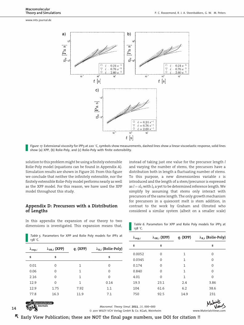
Figure 17. Extensional viscosity for iPP3 at 220 8C, symbols show measurements, dashed lines show a linear viscoelastic response, solid linesshow (a) XPP, (b) Rolie-Poly, and (c) Rolie-Poly with finite extensibility.

14

REa

www.mts-journal.de


solution to this problem might be using a finitely extensible

Rolie-Poly model (equations can be found in Appendix A).

Simulation results are shown in Figure 20. From this figure

we conclude that neither the infinitely extensible, nor the

finitely extensible Rolie-Poly model performs nearly as well

as the XPP model. For this reason, we have used the XPP

model throughout this study.

Table 6. Parameters for XPP and Rolie Poly models for iPP3 at

Appendix D: Precursors with a Distributionof Lengths

In this appendix the expansion of our theory to two

dimensions is investigated. This expansion means that,

Table 5. Parameters for XPP and Rolie Poly models for iPP2 at138 8C.

lrep,i l0R,i (XPP) qi (XPP) lR,i (Rolie-Poly)

s s s

0.01 0 1 0

0.06 0 1 0

2.16 0 1 0

12.9 0 1 0.14

12.9 1.75 7.92 1.1

77.8 16.3 11.9 7.1




instead of taking just one value for the precursor length l

and varying the number of stems, the precursors have a

distribution both in length a fluctuating number of stems.

To this purpose, a new dimensionless variable s is

introduced and the length of a stem/precursor is expressed

as l¼ sl0 with l0 a yet to be determined reference length. We

simplify by assuming that stems only interact with

precursors of the same length. The only growth mechanism

for precursors in a quiescent melt is stem addition, in

contrast to the work by Graham and Olmsted who

considered a similar system (albeit on a smaller scale)

138 8C.

lrep,i l0R,i (XPP) qi (XPP) lR,i (Rolie-Poly)

s s s

0.0052 0 1 0

0.0345 0 1 0

0.174 0 1 0

0.840 0 1 0

4.01 0 1 0

19.3 23.1 2.4 3.86

104 61.6 6.2 38.6

750 92.5 14.9 231

l. 2011, 20, 000–000



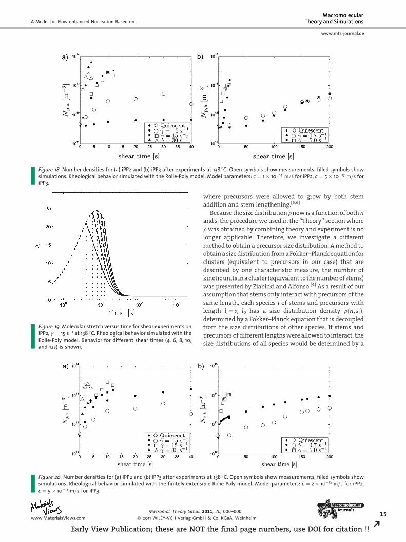
Figure 18. Number densities for (a) iPP2 and (b) iPP3 after experiments at 138 8C. Open symbols show measurements, filled symbols showsimulations. Rheological behavior simulated with the Rolie-Poly model. Model parameters: c ¼ 1� 10�14 m=s for iPP2, c ¼ 5� 10�17 m=s foriPP3.

Figure 19. Molecular stretch versus time for shear experiments oniPP2, _g ¼ 15 s�1 at 138 8C. Rheological behavior simulated with theRolie-Poly model. Behavior for different shear times (4, 6, 8, 10,and 12s) is shown.

Figure 20. Number densities for (a) iPP2 and (b) iPP3 after experimentsimulations. Rheological behavior simulated with the finitely extensc ¼ 5� 10�13 m=s for iPP3.






www.mts-journal.de

where precursors were allowed to grow by both stem

addition and stem lengthening.[5,6]

Because the size distribution r now is a function of both n

and s, the procedure we used in the ‘‘Theory’’ section where

r was obtained by combining theory and experiment is no

longer applicable. Therefore, we investigate a different

method to obtain a precursor size distribution. A method to

obtain a size distribution from a Fokker–Planck equation for

clusters (equivalent to precursors in our case) that are

described by one characteristic measure, the number of

kinetic units in a cluster (equivalent to the number of stems)

was presented by Ziabicki and Alfonso.[4] As a result of our

assumption that stems only interact with precursors of the

same length, each species i of stems and precursors with

length li¼ si l0 has a size distribution density rðn; siÞ,determined by a Fokker–Planck equation that is decoupled

from the size distributions of other species. If stems and

precursors of different lengths were allowed to interact, the

size distributions of all species would be determined by a

s at 138 8C. Open symbols show measurements, filled symbols showible Rolie-Poly model. Model parameters: c ¼ 2� 10�12 m=s for iPP2,

2011, 20, 000–000



16

REa

www.mts-journal.de


system of coupled Fokker–Planck equations with a large

number of unknown diffusion parameters, making the

model useless for current purposes.

The Fokker–Planck equation for species i is

rstðn;

rly V

@rðn; si; tÞ@t

� @

@n

Dgrðn; siÞ

�@rðn; si; tÞ

@n

þ rðn; si; tÞkT

@D~Fðn; siÞ@n

��¼ 0

(26)

where Dgr is the coefficient of growth diffusion and D~F is

the driving force of crystallization of a precursor with sizes

n, si. A steady state distribution density can be derived

following the same procedure as Ziabicki and Alfonso[4];

@rstðn; si; tÞ@t

¼ @

@n

Dgrðn; siÞ

�@rstðn; si; tÞ

@n

þ rstðn; si; tÞkT

@D~Fðn; siÞ@n

��¼ 0

(27)

@rstðn; siÞ@n

þ rstðn; siÞkT

@D~Fðn; siÞ@n

¼ C

Dgrðn; siÞ(28)

where C is a constant. We define Aðn; siÞ ¼1

kT

@~Fðn; siÞ@n

. As

an ansatz for the steady state distribution density we take

rst ¼ Fðn; siÞexp

Z nmax

nAðn0; siÞdn0

� �(29)

where nmax n� is a maximum for the precursor size

considered. Substituting into Equation (28) gives

@Fðn; siÞ@n

¼ C

Dgrðn; siÞexp �

Z nmax

nAðn0; siÞdn0

� �

Fðn; siÞ¼ Fðnmax; siÞ�C

Z nmax

n

1

Dgrðn0; siÞ

exp �Z nmax

n0Aðn00; siÞdn00

� �dn0

(30)

[4]
After applying the boundary conditions,
rstðn ¼ 1; siÞ ¼ r1ðsiÞ (31)

rstðn ¼ nmax n�; siÞ ¼ Fðnmax; siÞ ¼ 0 (32)

the steady state distribution for species i becomes

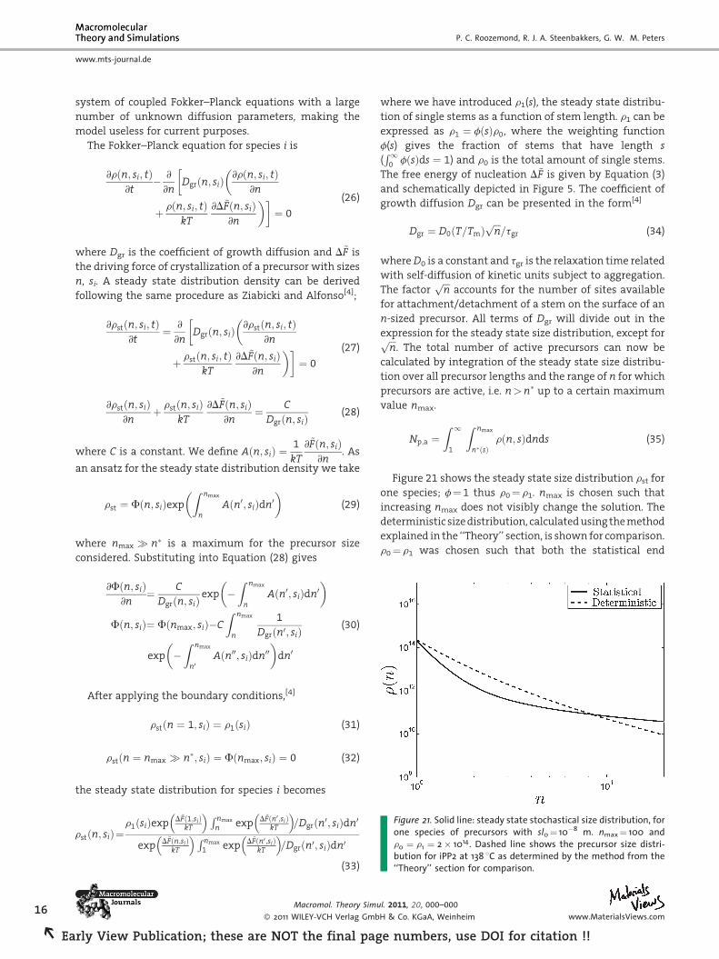
Figure 21. Solid line: steady state stochastical size distribution, forone species of precursors with sl0¼ 10�8 m. nmax¼ 100 andr0 ¼ r1 ¼ 2� 1014. Dashed line shows the precursor size distri-bution for iPP2 at 138 8C as determined by the method from the‘‘Theory’’ section for comparison.

siÞ¼r1ðsiÞexp D~Fð1;siÞ

kT

� R nmax

n exp D~Fðn0;siÞkT

� =Dgrðn0; siÞdn0

exp D~Fðn;siÞkT

� R nmax

1 exp D~Fðn0;siÞkT

� =Dgrðn0; siÞdn0

(33)




where we have introduced r1(s), the steady state distribu-

tion of single stems as a function of stem length. r1 can be

expressed as r1 ¼ fðsÞr0, where the weighting function

f(s) gives the fraction of stems that have length s

(R1

0 fðsÞds ¼ 1) and r0 is the total amount of single stems.

The free energy of nucleation D~F is given by Equation (3)

and schematically depicted in Figure 5. The coefficient of

growth diffusion Dgr can be presented in the form[4]

l. 2011

H & Co

e nu

Dgr ¼ D0 T=Tmð Þffiffiffinp

=tgr (34)

where D0 is a constant and tgr is the relaxation time related

with self-diffusion of kinetic units subject to aggregation.

The factorffiffiffinp

accounts for the number of sites available

for attachment/detachment of a stem on the surface of an

n-sized precursor. All terms of Dgr will divide out in the

expression for the steady state size distribution, except forffiffiffinp

. The total number of active precursors can now be

calculated by integration of the steady state size distribu-

tion over all precursor lengths and the range of n for which

precursors are active, i.e. n>n� up to a certain maximum

value nmax.

Np;a ¼Z 1

1

Z nmax

n�ðsÞrðn; sÞdnds (35)

Figure 21 shows the steady state size distribution rst for

one species; f¼ 1 thus r0¼ r1. nmax is chosen such that

increasing nmax does not visibly change the solution. The

deterministic size distribution, calculated using the method

explained in the ‘‘Theory’’ section, is shown for comparison.

r0¼ r1 was chosen such that both the statistical end

, 20, 000–000




www.mts-journal.de

deterministic size distributions have an equal amount of

precursors with size n¼ 1.

Unfortunately, at this moment this steady state dis-

tribution is of no use for the flow-enhanced nucleation

model presented in this study, for the following reasons.

First, the statistical model actually describes sporadic

nucleation, whereas the nucleation is mainly athermal in

flow-induced crystallization. Second, the main motivation

for deriving the statistical size distribution was to be able to

extend the present model to two dimensions. Because we

have no way to directly determine the weighting function

f(s), we cannot derive a unique function for the two-

dimensional precursor size distribution and therefore the

statistical approach, as the deterministic approach, is only

applicable to the one-dimensional case.

Acknowledgements: We would like to thank Prof. Dr. Han Slot forhelpful discussions on the statistical size distribution. Also, we arethankful to Dr. Markus Gahleitner for kindly providing isotacticty,nucleus number density data and nucleus growth rate data foriPP2. This work was supported by the Dutch TechnologyFoundation (STW), grant no. 08083.

Received: August 23, 2010; Revised: October 14, 2010; Publishedonline: DOI: 10.1002/mats.201000059

Keywords: crystallization; flow-enhanced nucleation; poly(pro-pylene) (PP); simulations; viscoelastic constitutive models

[1] S. Coppola, N. Grizzuti, Macromolecules 2001, 34, 5030.[2] N. Devaux, B. Monasse, J. M. Haudin, P. Moldenaers,

J. Vermant, Rheol. Acta. 2004, 43, 210.[3] A. Ziabicki, G. C. Alfonso, Macromol. Symp. 2002, 185, 211.[4] A. Ziabicki, G. C. Alfonso, Colloid Polym. Sci. 1994, 27, 1027.[5] R. S. Graham, P. D. Olmsted, Phys. Rev. Lett. 2009, 103.[6] R. S. Graham, P. D. Olmsted, Faraday Discuss. 2010, 144, 1.[7] G. Eder, H. Janeschitz-Kriegl, ‘‘Structure development during

processing: crystallization’’ in: Materials Science and Technol-ogy: Processing of Polymers - A Comprehensive Treatment, Vol.18, Wiley-VCH, Weinheim, 1997, pp 269–342.

[8] W. Schneider, A. Koppl, J. Berger, Int. Polym. Process. II 1988, 3,151.

[9] H. Zuidema, G. W. M. Peters, H. E. H. Meijer, Macromol. TheorySimul. 2001, 10, 447.

[10] H. Zuidema, PhD thesis, Eindhoven University of Technology,2000. available at www.mate.tue.nl/mate/pdfs/64.pdf.

[11] S. Vleeshouwers, H. E. H. Meijer, Rheol. Acta. 1996, 35, 391.[12] F. J. M. F. Custodio, PhD thesis, Eindhoven University of

Technology, 2009. available at www.mate.tue.nl/mate/pdfs/10371.pdf.





[13] F. J. M. F. Custodio, R. J. A. Steenbakkers, P. D. Anderson, G. W.M. Peters, H. E. H. Meijer, Macromol. Theory Simul. 2009, 18,469.

[14] R. J. A. Steenbakkers, G. W. M. Peters, Accepted in J. Rheol.2011.

[15] R. J. A. Steenbakkers, PhD thesis, Eindhoven University ofTechnology, 2009. available at www.mate.tue.nl/mate/pdfs/11262.pdf.

[16] J. W. Housmans, R. J. A. Steenbakkers, P. C. Roozemond, G. W.M. Peters, H. E. H. Meijer, Macromolecules 2009, 42, 5728.

[17] H. Janeschitz-Kriegl, Colloid Polym. Sci. 2003, 281, 1157.[18] H. Janeschitz-Kriegl, E. Ratajski, M. Stadlbauer, Rheol. Acta.

2003, 42, 355.[19] H. Janeschitz-Kriegl, E. Ratajski, Polymer 2005, 46, 3856.[20] M. Gahleitner, Personal communication, 2010.[21] F. H. M. Swartjes, PhD. Thesis, Eindhoven University of Tech-

nology, 2001. available at www.mate.tue.nl/mate/pdfs/901.pdf.

[22] R. J. A. Steenbakkers, G. W. M. Peters, Rheol. Acta. 2008, 47,643.

[23] M. Avrami, J. Chem. Phys. 1939, 7, 1103.[24] M. Avrami, J. Chem. Phys. 1940, 8, 212.[25] Z. Ma, R. J. A. Steenbakkers, J. Giboz, G. W. M. Peters, Rheol.

Acta., Published online on Dec 8 2010.[26] J. W. Housmans, PhD. Thesis, Eindhoven University of Tech-

nology, 2008. available at www.mate.tue.nl/mate/pdfs/10021.pdf.

[27] B. Monasse, J. M. Haudin, Colloid Polym. Sci. 1986, 264, 117.[28] M. Stadlbauer, H. Janeschitz-Kriegl, G. Eder, J. Rheol. 2004, 48,

631.[29] A. Mahendrasingam, C. Martin, W. Fuller, D. J. Blundell, R. J.

Oldman, J. L. Harvie, D. H. MacKerron, C. Riekel, Polymer 1999,40, 5553.

[30] E. L. Heeley, C. M. Fernyhough, R. S. Graham, P. D. Olmsted,N. J. Inkson, J. Emberey, D. J. Groves, T. C. B. McLeish, A. C.Morgovan, F. Meneau, W. Bras, A. J. Ryan, Macromolecules2006, 39, 5058.

[31] O. O. Mykhaylyk, P. Chambom, R. S. Graham, J. P. A. Fair-clough, P. D. Olmsted, A. J. Ryan, Macromolecules 2008, 41,1901.

[32] L. Yang, R. H. Somani, I. Sics, B. S. Hsiao, R. Kolb, H. Fruitwala,C. Ong, Macromolecules 2004, 37, 4845.

[33] J. Baert, P. van Puyvelde, Macromolecules 2006, 39, 9215.[34] J. A. Martins, W. Zhang, A. M. Brito, Macromolecules 2006, 39,

7626.[35] G. W. M. Peters, F. P. T. Baaijens, J. Non-Newton. Fluid Mech.

1997, 68, 205.[36] A. I. Leonov, Rheol. Acta. 1976, 15, 85.[37] A. I. Leonov, J. Non-Newton. Fluid Mech. 1987, 25, 1.[38] A. I. Leonov, J. Non-Newton. Fluid Mech. 1992, 42, 323.[39] P. Rubio, M. H. Wagner, J. Rheol. 1999, 43, 1709.[40] K. K. Kabanemi, J. F. Hetu, Rheol. Acta. 2009, 48, 801.[41] H. Giesekus, J. Non-Newton. Fluid Mech. 1982, 11, 69.[42] H. Giesekus, Rheol. Acta. 1982, 21, 366.[43] W. M. H. Verbeeten, G. W. M. Peters, F. P. T. Baaijens, J. Non-

Newton. Fluid Mech. 2004, 117, 73.[44] A. E. Likhtman, R. S. Graham, J. Non-Newton. Fluid Mech. 2003,

114, 1.

2011, 20, 000–000



Documents

A Model for Flow-enhanced Nucleation Based on Fibrillar Dormant Precursors