Computers & Operations Research 39 (2012) 687–697

Contents lists available at ScienceDirect

Computers & Operations Research

0305-05

doi:10.1

� Corr

E-m

journal homepage: www.elsevier.com/locate/caor

A modified artificial bee colony algorithm

Wei-feng Gao �, San-yang Liu

Department of Mathematics, Xidian University, Xi’an, Shannxi 710071, PR China

a r t i c l e i n f o

Available online 25 June 2011

Keywords:

Artificial bee colony algorithm

Initial population

Solution search equation

Differential evolution

48/$ - see front matter & 2011 Elsevier Ltd. A

016/j.cor.2011.06.007

esponding author.

ail address: gaoweifeng2004@126.com (W.-f.

a b s t r a c t

Artificial bee colony algorithm (ABC) is a relatively new optimization technique which has been shown

to be competitive to other population-based algorithms. However, there is still an insufficiency in ABC

regarding its solution search equation, which is good at exploration but poor at exploitation. Inspired

by differential evolution (DE), we propose an improved solution search equation, which is based on that

the bee searches only around the best solution of the previous iteration to improve the exploitation.

Then, in order to make full use of and balance the exploration of the solution search equation of ABC

and the exploitation of the proposed solution search equation, we introduce a selective probability P

and get the new search mechanism. In addition, to enhance the global convergence, when producing

the initial population, both chaotic systems and opposition-based learning methods are employed. The

new search mechanism together with the proposed initialization makes up the modified ABC (MABC for

short), which excludes the probabilistic selection scheme and scout bee phase. Experiments are

conducted on a set of 28 benchmark functions. The results demonstrate good performance of MABC in

solving complex numerical optimization problems when compared with two ABC-based algorithms.

& 2011 Elsevier Ltd. All rights reserved.

1. Introduction

Learning from life system, people have developed manyoptimization computation methods to solve complicated pro-blems in recent decades, such as genetic algorithm (GA) inspiredby the Darwinian law of survival of the fittest [1], particle swarmoptimization (PSO) inspired by the social behavior of bird flockingor fish schooling [2], ant colony optimization (ACO) inspired bythe foraging behavior of ant colonies [3], and biogeography-basedoptimization (BBO) inspired by the migration behavior of islandspecies [4]. We call this kind of algorithms for scientific computa-tion as ‘‘artificial-life computation’’ [5]. Artificial bee colonyalgorithm (ABC) is such a new computation technique developedby Karaboga [6] based on simulating the foraging behavior ofhoney bee swarm. Numerical comparisons demonstrated that theperformance of ABC is competitive to other population-basedalgorithms with an advantage of employing fewer control para-meters [7–9]. Due to its simplicity and ease of implementation,ABC has captured much attention and has been applied to solvemany practical optimization problems [10–12] since its inventionin 2005.

However, similar to other evolutionary algorithms, ABC alsofaces up to some challenging problems. For example, the converg-ence speed of ABC is typically slower than those of representative

ll rights reserved.

Gao).

population-based algorithms (e.g., differential evolution (DE) [13] andPSO) when handling those unimodal problems [9]. What is more, ABCcan easily get trapped in the local optima when solving complexmultimodal problems [9]. The reasons are as follows. It is well knownthat both exploration and exploitation are necessary for a population-based optimization algorithm. In the optimization algorithms, theexploration refers to the ability to investigate the various unknownregions in the solution space to discover the global optimum. While,the exploitation refers to the ability to apply the knowledge of theprevious good solutions to find better solutions. In practice, theexploration and exploitation contradicts to each other. In order toachieve good performances on problem optimizations, the twoabilities should be well balanced. While, the solution search equationof ABC which is used to generate new candidate solutions based onthe information of previous solutions, is good at exploration but poorat exploitation [14], which results in the above two insufficiencies.

Therefore, accelerating convergence speed and avoiding thelocal optima have become two most important and appealinggoals in ABC research. A number of variant ABC algorithms have,hence, been proposed to achieve these two goals [14–16].However, so far, it is seen to be difficult to simultaneously achieveboth goals. For example, the chaotic ABC algorithm (CABC) in [16]focuses on avoiding the local optima, but brings in a more extrafunction evaluations in chaotic search as a result.

To achieve the both goals, inspired by DE, we propose animproved solution search equation, which is based on that the beesearches only around the best solution of the previous iteration toimprove the exploitation. Then, in order to make full use of and

W.-F. Gao, S.-Y. Liu / Computers & Operations Research 39 (2012) 687–697688

balance the exploration of the solution search equation of ABC andthe exploitation of the proposed solution search equation, weintroduce a selective probability P and get the new search mechan-ism. In addition, to enhance the global convergence, when producingthe initial population, both chaotic systems and opposition-basedlearning method are employed. The new search mechanismtogether with the proposed initialization makes up the modifiedABC (MABC for short), which excludes the probabilistic selectionscheme and scout bee phase. The rest of this paper is organized asfollows. Section 2 summarizes ABC. The improved ABC algorithm ispresented in Section 3. Section 4 presents and discusses theexperimental results. Finally, the conclusion is drawn in Section 5.

2. Artificial bee colony algorithm

Artificial bee colony algorithm (ABC), proposed by Karaboga in2005 for real-parameter optimization, is a recently introducedoptimization algorithm which simulates the foraging behavior ofa bee colony [6]. ABC classifies the foraging artificial bees intothree groups, namely, employed bees, onlooker bees and scoutbees. Half of the colony consists of employed bees, and the otherhalf includes onlooker bees. Employed bees search the foodaround the food source in their memory, meanwhile they passtheir food information to onlooker bees. Onlooker bees tend toselect good food sources from those founded by the employedbees, then further search the foods around the selected foodsource. Scout bees are translated from a few employed bees,which abandon their food sources and search new ones.

Similar to the other population-based algorithms, ABC is aniterative process. The units of the basic ABC can be explained asfollows:

2.1. Initialization of the population

The initial population of solutions is filled with SN number ofrandomly generated n-dimensional real-valued vectors (i.e., foodsources). Let Xi ¼ fxi,1,xi,2, . . . ,xi,ng represent the ith food source inthe population, and then each food source is generated as follows:

xi,j ¼ xmin,jþrandð0,1Þðxmax,j�xmin,jÞ, ð2:1Þ

where i¼ 1,2, � � � ,SN,j¼ 1,2, � � � ,n. xmin,j and xmax,j are the lowerand upper bounds for the dimension j, respectively. These foodsources are randomly assigned to SN number of employed beesand their fitnesses are evaluated.

2.2. Initialization of the bee phase

At this stage, each employed bee Xi generates a new foodsource Vi in the neighborhood of its present position by usingsolution search equation as follows:

vi,j ¼ xi,jþfi,jðxi,j�xk,jÞ, ð2:2Þ

where kAf1,2, � � � ,SNg and jAf1,2, � � � ,ng are randomly chosenindexes; k has to be different from i; fi,j is a random number inthe range [�1, 1].

Once Vi is obtained, it will be evaluated and compared to Xi. Ifthe fitness of Vi is equal to or better than that of Xi, Vi will replaceXi and become a new member of the population; otherwise Xi isretained. In other words, a greedy selection mechanism isemployed between the old and candidate solutions.

2.3. Calculating probability values involved in probabilistic selection

After all employed bees complete their searches, they sharetheir information related to the nectar amounts and the positions

of their sources with the onlooker bees on the dance area. Anonlooker bee evaluates the nectar information taken from allemployed bees and chooses a food source site with a probabilityrelated to its nectar amount. This probabilistic selection dependson the fitness values of the solutions in the population. A fitness-based selection scheme might be a roulette wheel, ranking based,stochastic universal sampling, tournament selection or anotherselection scheme. In basic ABC, roulette wheel selection schemein which each slice is proportional in size to the fitness value isemployed as follows:

pi ¼ fi

XSN

j ¼ 1

fj

,, ð2:3Þ

where fi is the fitness value of solution i. Obviously, the higher thefi is, the more probability that the ith food source is selected.

2.4. Onlooker bee phase

An onlooker bee evaluates the nectar information taken from allthe employed bees and selects a food source Xi depending on itsprobability value pi. Once the onlooker has selected her food sourceXi, she produces a modification on Xi by using Eq. (2.2).As in the case of the employed bees, if the modified food sourcehas a better or equal nectar amount than Xi, the modified foodsource will replace Xi and become a new member in the population.

2.5. Scout bee phase

If a food source Xi cannot be further improved through apredetermined number of trials limit, the food source is assumedto be abandoned, and the corresponding employed bee becomes ascout. The scout produces a food source randomly as follows:

xi,j ¼ xmin,jþrandð0,1Þðxmax,j�xmin,jÞ, ð2:4Þ

where j¼ 1,2, � � � ,n.

2.6. Main steps of the artificial bee colony algorithm

Based on the above explanation of initializing the algorithmpopulation, employed bee phase, probabilistic selection scheme,onlooker bee phase and scout bee phase, the pseudo-code of theABC algorithm is given below:

Algorithm 1 (Artificial bee colony algorithm).

01: Initialize the population of solutions xi,j, i¼ 1,2 � � � SN,

j¼ 1,2 � � �n, triali ¼ 0, triali ¼ 0 is the non-improvementnumber of the solution Xi, used for abandonment

02: Evaluate the population03: cycle¼104: repeat

{– – Produce a new food source population for employedbees – –}

06: for i¼ 1 to SN do07: Produce a new food source Vi for the employed bee

of the food source Xi using (2.2) and evaluate itsquality

08: Apply a greedy selection process between Vi and Xi

and select the better one

09: If solution Xi does not improve triali ¼ trialiþ1,

otherwise triali ¼ 010: end for11: Calculate the probability values pi by (2.3) for the

solutions using fitness values{– – Produce a new food source population for onlookerbees – –}

W.-F. Gao, S.-Y. Liu / Computers & Operations Research 39 (2012) 687–697 689

12: t¼ 0,i¼ 113: repeat14: if randomopi then15: Produce a new Vi food source by (2.2) for onlooker

bee16: Apply a greedy selection process between Vi and Xi

and select the better one

17: If solution Xi does not improve triali ¼ trialiþ1,

otherwise triali ¼ 018: t¼ tþ1

19: endif20: until (t¼SN)

{– – Determine Scout – –}

21: if maxðtrialiÞ4 limit then22: Replace Xi with a new randomly produced solution

by (2.4)23: end if24: Memorize the best solution achieved so far25: cycle¼cycleþ126: until (cycle¼Maximum Cycle Number)

3. Modified artificial bee colony algorithm

3.1. Initial population

Population initialization is a crucial task in evolutionary algo-rithms because it can affect the convergence speed and the qualityof the final solution. If no information about the solution is available,then random initialization is the most commonly used method togenerate candidate solutions (initial population). Owing to therandomness and sensitivity dependence on the initial conditionsof chaotic maps, chaotic maps have been used to initialize thepopulation so that the search space information can be extracted toincrease the population diversity in [16]. At the same time, accord-ing to [17], replacing the random initialization with the opposition-based population initialization can get better initial solutions andthen accelerate convergence speed. So this paper proposes a novelinitialization approach which employs opposition-based learningmethod and chaotic systems to generate initial population. Here,sinusoidal iterator is selected and its equation is defined as follows:

chkþ1 ¼ sinðpchkÞ,chkAð0,1Þ,k¼ 0,1,2, . . . ,K , ð3:1Þ

where k is the iteration counter and K is the preset maximum numberof chaotic iterations. The mapped variables in Eq. (3.1) can distribute

Table 1Effect of the selective probability P on the performance of MABC.

Algorithm Sphere Rosebrock

MABC (P¼0.0) Mean 1.86e�36 3.07e�00

SD 1.46e�36 3.45e�00

MABC (P¼0.1) Mean 2.57e�35 3.04e�00

SD 2.44e�35 3.95e�00

MABC (P¼0.3) Mean 5.48e�34 1.01e�00

SD 3.87e�34 1.41e�00

MABC (P¼0.5) Mean 7.57e�33 1.67e�00

SD 3.28e�33 1.43e�00

MABC (P¼0.7) Mean 9.43e�32 6.11e�01

SD 6.67e�32 4.55e�01

MABC (P¼0.9) Mean 2.47e�30 9.55e�01

SD 2.53e�30 1.03e�00

MABC (P¼1.0) Mean 4.33e�30 1.47e�00

SD 4.21e�30 1.22e�00

in search space with ergodicity, randomness and irregularity. Basedon these operations, we propose the following algorithm to generateinitial population which can be used instead of a pure randominitialization.

Algorithm 2 (A novel initialization approach).

01: Set the maximum number of chaotic iteration KZ300,the population size SN, and the individual counter

i¼ 1,j¼ 1{– – chaotic systems – –}

03: for i¼1 to SN do04: for j¼1 to n do05: Randomly initialize variables ch0,jA ð0,1Þ, set

iteration counter k¼006: for k¼1 to K do07: chkþ1,j ¼ sinðpchk,jÞ

08: end for09: xi,j ¼ xmin,jþchk,jðxmax,j�xmin,jÞ

10: end for11: end for

{– – Opposition-based learning method – –}

13: Set the individual counter i¼ 1,j¼ 114: for i¼1 to SN do15: for j¼ 1 to n do16: oxi,j ¼ xmin,jþxmax,j�xi,j

17: end for18: end for19: Selecting SN fittest individuals from set the fXðSNÞ [ OXðSNÞg

as initial population.

3.2. A modified search equation

Differential evolution (DE) [13] has been shown to be a simpleyet efficient evolutionary algorithm for many optimization pro-blems in real-world applications. It follows the general procedureof an evolutionary algorithm. After initialization, DE enters a loopof evolutionary operations: mutation, crossover, and selection.There are several variant DE algorithms which are different inthat their mutation strategies are adopted differently. The follow-ing is a mutation strategy frequently used in the literature:

DE=best=1 : Vi ¼ XbestþFðXr1�Xr2Þ, ð3:2Þ

where i¼ f1,2, � � � ,SNg and r1 and r2 are mutually differentrandom integer indices selected from f1,2, � � � ,SNg. F, commonlyknown as scaling factor or amplification factor, is a positive real

Griewank Rastrigin NC-Rastrigin Ackley

3.28e�04 3.32e�02 0 2.88e�14

1.83e�03 1.78e�01 0 3.63e�15

2.46e�04 6.22e�02 0 3.00e�14

1.36e�03 2.41e�01 0 1.42e�15

4.00e�05 5.02e�03 0 3.12e�14

2.15e�04 7.05e�02 0 1.77e�15

0 0 0 3.59e�14

0 0 0 3.39e�15

0 0 0 4.13e�14

0 0 0 2.17e�15

3.54e�18 0 0 5.27e�14

7.28e�17 0 0 6.19e�15

6.66e�15 0 0 6.62e�14

3.44e�14 0 0 1.10e�14

W.-F. Gao, S.-Y. Liu / Computers & Operations Research 39 (2012) 687–697690

number, typically less than 1.0 that controls the rate at which thepopulation evolves.

The best solutions in the current population are very usefulsources that can be used to improve the convergence performance.The example is the DE/best/1, where the best solutions explored inthe history are used to direct the movement of the currentpopulation. Based on the variant DE algorithm and the property ofABC, the solution search equation is devised as follows:

ABC=best=1 : vi,j ¼ xbest,jþfi,jðxr1,j�xr2,jÞ, ð3:3Þ

where the indices r1 and r2 are mutually exclusive integers randomlychosen from f1,2, � � � ,SNg, and different from the base index i; Xbest isthe best individual vector with the best fitness in the currentpopulation and jAf1,2, . . . ,ng is randomly chosen indexes; fi,j is arandom number in the range [�1, 1]. In Eq. (2.2), the coefficient fi,j isa uniform random number in [�1, 1] and xk,j is a random individual

Table 2Benchmark functions used in experiments.

Function

f1ðXÞ ¼Pn

i ¼ 1 x2i

f2ðXÞ ¼Pn

i ¼ 1ð106Þði�1Þ=ðn�1Þx2

i

f3ðXÞ ¼Pn

i ¼ 1 ix2i

f4ðXÞ ¼Pn

i ¼ 1 jxijðiþ1Þ

f5ðXÞ ¼Pn

i ¼ 1 jxijþQn

i ¼ 1 jxij

f6ðXÞ ¼maxifjxij,1r irng

f7ðXÞ ¼Pn

i ¼ 1ðbxiþ0:5cÞ2

f8ðXÞ ¼Pn

i ¼ 1 ix4i

f9ðXÞ ¼Pn

i ¼ 1 ix4i þrandom½0,1Þ

f10ðXÞ ¼Pn�1

i ¼ 1½100ðxiþ1�x2i Þ

2þðxi�1Þ2�

f11ðXÞ ¼ ½x2i �10 cosð2pxiÞþ10�

f12ðXÞ ¼ ½y2i �10 cosð2pyiÞþ10�

yi ¼

xi jxijo 12

roundð2xiÞ

2jxijZ

12

8><>:

f13ðXÞ ¼1

4000

Pni ¼ 1 x2

i �Qn

i ¼ 1 cosxiffiffi

ip

� �þ1

f14ðXÞ ¼ 418:98288727243369nn�Pn

i ¼ 1 xi sinðffiffiffiffiffiffiffijxijpÞ

f15ðXÞ ¼�20 exp �0:2

ffiffiffiffiffiffiffiffiffiffiffiffiffiffiffiffiffiffiffiffiffiffi1

n

Pni ¼ 1 x2

i

r !�exp

1

n

Pni ¼ 1 cosð2pxiÞ

� �þ20þe

f16ðXÞ ¼pn f10 sin2

ðpy1ÞþPn�1

i ¼ 1ðyi�1Þ2½1þ10 sin2ðpyiþ1Þ�

þðyn�1Þ2gþPn

i ¼ 1 uðxi,10,100,4Þ

yi ¼ 1þ 14 ðxiþ1Þ uxi ,a,k,m ¼

kðxi�aÞm xi 4a

0 �arxi ra

kð�xi�aÞm xi o�a

8><>:

f17ðXÞ ¼1

10 fsin2ðpx1Þþ

Pn�1i ¼ 1ðxi�1Þ2½1þsin2

ð3pxiþ1Þ�

þðxn�1Þ2½1þsin2ð2pxiþ1Þ�gþ

Pni ¼ 1 uðxi ,5,100,4Þ

f18ðXÞ ¼Pn

i ¼ 1 jxi � sinðxiÞþ0:1 � xij

f19ðXÞ ¼Pn�1

i ¼ 1ðxi�1Þ2½1þsin2ð3pxiþ1Þ�þsin2

ð3px1Þ

þjxn�1j½1þsin2ð3pxnÞ�

f20ðXÞ ¼PD

i ¼ 1ðPkmax

k ¼ 0½ak cosð2pbkðxiþ0:5ÞÞ�Þ�D

Pkmax

k ¼ 0½ak

cosð2pbk0:5Þ�,a¼ 0:5,b¼ 3,kmax ¼ 20

f21ðXÞ ¼ 0:5þsin2ð

ffiffiffiffiffiffiffiffiffiffiffiffiffiffiffiffiffiffiffiPni ¼ 1 x2

i

q�0:5

ð1þ0:001ðPn

i ¼ 1 x2i ÞÞ

2

f22ðXÞ ¼1n

Pni ¼ 1ðx

4i �16x2

i þ5xiÞ

f23ðXÞ ¼�Pn

i ¼ 1 sinðxiÞ sin20 i� x2i

p

!

f24ðXÞ ¼Pn

i ¼ 1 z2i Z ¼ X�O

f25ðXÞ ¼ ½z2i �10 cosð2pziÞþ10� Z ¼ X�O

f26ðXÞ ¼1

4000

Pni ¼ 1 z2

i �Qn

i ¼ 1 cosð ziffiip Þþ1 Z ¼ X�O

f27ðXÞ ¼�20 exp �0:2

ffiffiffiffiffiffiffiffiffiffiffiffiffiffiffiffiffiffiffiffiffiffi1

n

Pni ¼ 1 z2

i

r !�exp

1

n

Pni ¼ 1 cosð2pziÞ

� �Z ¼ X�O

f28ðXÞ ¼Pn

i ¼ 1 jzi � sinðziÞþ0:1 � zij Z ¼ X�O

in the population. Therefore, the solution search dominated by Eq.(2.2) is random enough for exploration. In other words, the solutionsearch equation described by Eq. (2.2) is good at exploration but poorat exploitation. However, according to Eq. (3.3), ABC/best/1 can drivethe new candidate solution only around the best solution of theprevious iteration. Therefore, the proposed solution search equationdescribed by Eq. (3.3) can increase the exploitation of ABC.

3.3. The proposed approach

From the above explanation, it is clear that ABC/best/1 has agood capacity of the exploitation. Unfortunately, ABC/best/1 canreduce the exploration of ABC. If all bees produce new foodsources using (3.3), the algorithm can easily get trapped in thelocal optima when solving complex multimodal problems. Inother words, ABC which is good at exploration but poor at

Search range Min

[�100,100]n 0

[�100,100]n 0

[�10,10]n 0

[�10,10]n 0

[�10,10]n 0

[�100,100]n 0

[�100,100]n 0

[�1.28,1.28]n 0

[�1.28,1.28]n 0

[�10,10]n 0

[�5.12,5.12]n 0

[�5.12,5.12]n 0

[�600,600]n 0

[�500,500]n 0

[�32,32]n 0

[�50,50]n 0

[�50,50]n 0

[�10,10]n 0

[�10,10]n 0

[�0.5,0.5]n 0

[�100,100]n 0

[�5,5]n�78.33236

½0,p�n �99.2784 for n¼100

[�100,100]n 0

[�5.12,5.12]n 0

[�600,600]n 0

[�32,32]n 0

[�10,10]n 0

W.-F. Gao, S.-Y. Liu / Computers & Operations Research 39 (2012) 687–697 691

exploitation results in a slow convergence. While ABC/best/1,which is good at exploitation but poor at exploration, cannotavoid premature convergence. To address this contradiction, wepropose the new search mechanism which introduces the selec-tive probability P to balance the exploration of the solution searchequation (2.2) and the exploitation of the modified solutionsearch equation (3.3). The new search mechanism withAlgorithm 2 makes up MABC. Based on the above explanation,the pseudo-code of MABC is given below:

Algorithm 3 (Modified artificial bee colony algorithm).

01: Set the population size SN, give the maximum number offunction evaluations, Max:FE

02: Perform Algorithm 2 to create an initial population

fXiji¼ 1,2, � � � ,SNg, calculate the function values of the

population ffiji¼ 1,2, � � � ,SNg

03: While (stopping criterion is not met, namelyFEoMax:FE) do

04: for i¼ 1 to SN do{– – Produce a new food source using the new searchmechanism– –}

06: Choose Xr1,Xr2 randomly from the current population,The indices r1,r2 are mutually exclusive integers

Table 3Best, worst, median, mean and standard deviation values obtained by ABC and MABC th

Fun Dim Best Worst

f1 30 ABC 2.02e�10 1.07e�09

MABC 1.69e�32 2.48e�31

60 ABC 3.49e�10 3.27e�09

MABC 9.29e�30 1.55e�28

100 ABC 3.87e�10 3.11e�09

MABC 4.65e�28 2.63e�27

f2 30 ABC 2.65e�07 1.32e�05

MABC 2.55e�29 1.99e�27

60 ABC 2.14e�07 6.25e�06

MABC 3.65e�26 8.69e�25

100 ABC 4.00e�07 6.46e�06

MABC 3.17e�24 3.73e�24

f3 30 ABC 9.03e�12 4.62e�11

MABC 3.57e�33 5.29e�32

60 ABC 7.95e�11 3.17e�10

MABC 5.61e�30 3.29e�29

100 ABC 2.82e�10 2.85e�09

MABC 1.50e�28 8.74e�28

f4 30 ABC 1.34e�18 4.29e�16

MABC 1.26e�74 1.34e�68

60 ABC 4.88e�11 7.62e�10

MABC 5.16e�65 9.54e�62

100 ABC 2.52e�08 2.05e�06

MABC 7.76e�52 8.74e�48

f5 30 ABC 1.28e�06 2.63e�06

MABC 8.41e�18 4.09e�17

60 ABC 5.77e�06 9.29e�06

MABC 5.30e�16 8.72e�16

100 ABC 1.28e�06 1.59e�05

MABC 2.08e�15 6.63e�15

f6 30 ABC 1.30eþ01 2.07eþ01

MABC 9.16e�00 1.42eþ01

60 ABC 3.79eþ01 4.65eþ01

MABC 2.92eþ01 4.03eþ01

100 ABC 5.30eþ01 6.14eþ01

MABC 5.70eþ01 6.23eþ01

f7 30 ABC 0 0

MABC 0 0

60 ABC 0 0

MABC 0 0

100 ABC 0 0

MABC 0 0

randomly chosen from the range ½1,SN�, which are alsodifferent from the index i

07: Randomly choose j from f1,2, � � � ,ng and produce

fi,jA ½�1,1�

08: Generate a new food source Vi according to

vi,j ¼ xbest,jþfi,jðxr1,j�xr2,jÞ

09: if f ðViÞo f ðXiÞ then10: Xi ¼ Vi

11: else then12: if randð0,1ÞoP then14: Randomly choose j from f1,2, � � � ,ng,

kAf1,2, � � � ,SNg which has to be different from i

and produce fi,jA ½�1,1�

15: Generate a new food source Vi according to

vi,j ¼ xi,jþfi,jðxi,j�xk,jÞ

16: if f ðViÞo f ðXiÞ then17: Xi ¼ Vi

18: endif19: end if20: end if21: end for22: end while (FE¼Max:FE)

rough 30 independent runs on function from f1 to f7.

Median Mean SD Significant

2.02e�10 5.21e�10 2.46e�10

1.80e�32 9.43e�32 6.67e�32 þ

3.27e�09 1.09e�09 9.37e�10

4.68e�29 6.03e�29 4.31e�29 þ

3.87e�10 1.64e�09 9.85e�10

1.86e�27 1.43e�27 8.12e�28 þ

7.71e�07 4.10e�06 3.85e�06

1.99e�27 3.66e�28 5.96e�28 þ

4.53e�06 2.31e�06 2.18e�06

3.65e�26 3.51e�25 2.72e�25 þ

1.37e�06 1.79e�06 1.63e�06

3.17e�24 3.52e�24 2.47e�25 þ

1.56e�11 2.22e�11 1.14e�11

4.62e�33 2.10e�32 1.56e�32 þ

3.17e�10 1.89e�10 9.14e�11

6.24e�30 1.39e�29 8.84e�30 þ

4.21e�10 1.25e�09 9.75e�10

1.72e�28 4.46e�28 2.08e�28 þ

1.82e�16 1.45e�16 1.55e�16

7.02e�71 2.70e�69 5.38e�69 þ

4.88e�11 2.14e�10 2.75e�10

3.59e�64 3.00e�62 3.87e�62 þ

6.75e�08 4.83e�07 7.88e�07

8.01e�52 1.92e�48 3.42e�48 þ

1.28e�06 1.83e�06 4.80e�07

8.41e�18 2.40e�17 9.02e�18 þ

6.81e�06 7.23e�06 1.28e�06

8.33e�16 6.96e�16 1.20e�16 þ

1.29e�05 1.30e�05 1.93e�06

6.46e�15 4.41e�15 1.50e�15 þ

1.52eþ01 1.80eþ01 2.25e�00

1.26eþ01 1.02eþ01 1.49e�00 þ

4.18eþ01 4.22eþ01 2.73e�00

3.80eþ01 3.77eþ01 3.14e�00 þ

5.30eþ01 5.76eþ01 2.74e�00

5.76eþ01 5.98eþ01 1.60e�00 .

0 0 0

0 0 0 NA

0 0 0

0 0 0 NA

0 0 0

0 0 0 NA

W.-F. Gao, S.-Y. Liu / Computers & Operations Research 39 (2012) 687–697692

3.4. Adjusting the selective probability P

Note that the parameter P plays an important role in balancing theexploration and exploitation of the candidate solution search. When P

takes 0, only Eq. (3.3) is at work. When P increases from 0 to 1, theexploration of Eq. (2.2) will also increase correspondingly. However, P

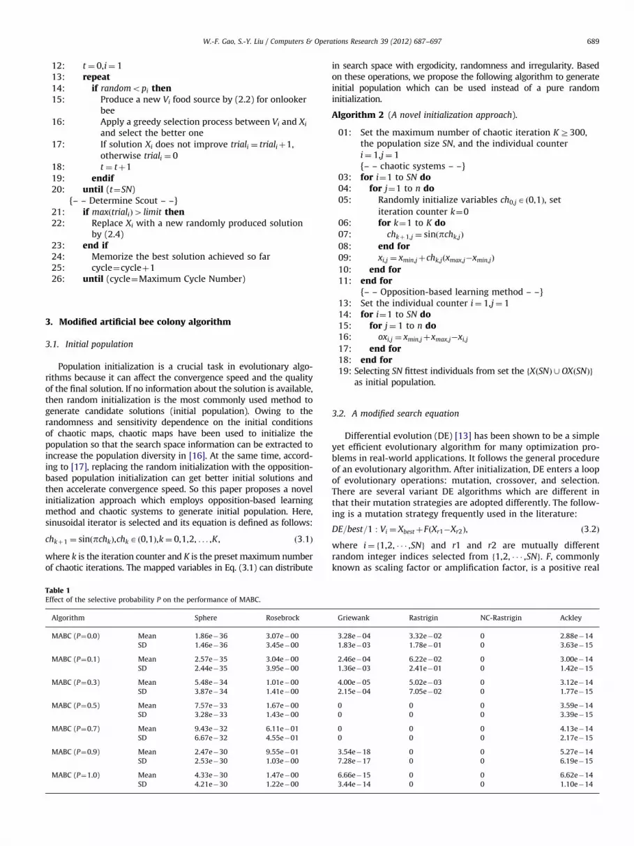
should not be too large because the large value of P might weaken theexploitation of the algorithm. Therefore the selective probabilityparameter P needs to be tuned. In this section, six different kinds ofthirty-dimensional (30-D) test functions are used to investigate theimpact of this parameter. They are the Sphere, Rosenbrock, Griewank,Rastrigin, NC-Rastrigin and Ackley functions [15] as defined inSection 4. MABC runs 30 times on each of these functions, and themean and standard deviation values of the final results are pre-sented in Table 1. As all test functions are minimization problems,the smaller the final result, the better it is. From Table 1, we canobserve that P can influence the results. When P is 0, we obtain afaster convergence velocity and better results on the Sphere andAckley functions. For the other four test functions, better results areobtained when P is around 0.7. At the same time, P has a smallereffect on the Sphere and Ackley functions than for the other four testfunctions. Hence, in our experiments, the selective probability P is

Table 4Best, worst, median, mean and standard deviation values obtained by ABC and MABC

Fun Dim Best Worst

f8 30 ABC 1.26e�29 1.86e�28

MABC 8.80e�69 5.97e�67

60 ABC 4.90e�28 2.00e�26

MABC 4.49e�64 2.37e�61

100 ABC 1.31e�26 1.41e�25

MABC 3.99e�61 1.56e�59

f9 30 ABC 6.03e�02 1.27e�01

MABC 1.84e�02 4.58e�02

60 ABC 1.87e�01 2.65e�01

MABC 9.20e�02 1.33e�01

100 ABC 3.96e�01 4.92e�01

MABC 1.64e�01 2.56e�01

f10 30 ABC 2.12e�02 2.20e�00

MABC 4.09e�02 1.95e�00

60 ABC 1.88e�01 5.75e�00

MABC 2.17e�01 5.26e�00

100 ABC 5.48e�01 3.94e�00

MABC 5.13e�01 7.77e�00

f11 30 ABC 3.58e�10 1.46e�01

MABC 0 0

60 ABC 3.21e�10 1.99e�00

MABC 0 0

100 ABC 5.40e�09 1.99e�00

MABC 0 0

f12 30 ABC 8.96e�10 1.00e�00

MABC 0 0

60 ABC 2.17e�07 3.025e�00

MABC 0 0

100 ABC 2.00e�00 7.21e�00

MABC 0 0

f13 30 ABC 4.74e�12 1.35e�07

MABC 0 0

60 ABC 7.99e�12 1.05e�09

MABC 0 0

100 ABC 6.29e�13 3.05e�08

MABC 0 0

f14 30 ABC 1.54e�06 2.37eþ02

MABC �1.81e�12 0

60 ABC 3.55eþ02 7.69eþ02

MABC 2.91e�11 3.63e�11

100 ABC 7.81eþ02 1.55eþ03

MABC 1.09e�10 1.23e�10

set at 0.7 for all test functions. Above all, the proposed approach isable to reach the balance between exploration and exploitation.

4. Experimental studies on function optimization problems

4.1. Benchmark functions and parameter settings

In this section, MABC is applied to minimize a set of 26scalable benchmark functions of dimensions D¼30, 60 or 100[9,14,17] and a set of two functions of higher dimension D¼100,200 or 300 [17], as shown in Table 2.

Summarized in Table 2 are the 28 scalable benchmark func-tions. f1�f6 and f8 are continuous unimodal functions. f7 is adiscontinuous step function, and f9 is a noisy quartic function. f10

is the Rosenbrock function which is unimodal for D¼2 and 3 butmay have multiple minima in high dimension cases [18]. f112f23

are multimodal and the number of their local minima increasesexponentially with the problem dimension. f242f28 are shiftedfunctions and O is a randomly generated shift vector located insearch range. In addition, f14 is the only bound-constrainedfunction investigated in this paper.

through 30 independent runs on function from f8 to f14.

Median Mean SD Significant

1.64e�29 5.51e�29 6.70e�29

1.01e�68 1.45e�67 2.28e�67 þ

4.90e�28 6.53e�27 7.23e�27

2.37e�61 5.00e�62 9.38e�62 þ

1.34e�26 5.65e�26 4.90e�26

3.99e�61 5.72e�60 5.32e�60 þ

7.67e�02 8.74e�02 1.77e�02

4.48e�02 3.71e�02 8.53e�03 þ

2.43e�01 2.39e�01 2.86e�02

1.21e�01 1.14e�01 1.16e�02 þ

4.70e�01 4.55e�01 3.20e�02

2.56e�01 2.31e�01 2.79e�02 þ

5.56e�01 4.23e�01 4.34e�01

2.34e�01 6.11e�01 4.55e�01 .

1.80e�00 1.86e�00 1.36e�00

1.30e�00 1.51e�00 1.34e�00 þ

6.33e�01 1.59e�00 1.23e�00

6.71e�01 1.98e�00 1.30e�00 .

5.50e�10 4.81e�03 2.57e�02

0 0 0 þ

1.28e�05 3.71e�01 5.97e�01

0 0 0 þ

1.99e�00 1.10e�00 8.21e�01

0 0 0 þ

1.77e�08 1.12e�01 2.97e�01

0 0 0 þ

1.09e�00 1.47e�00 9.47e�01

0 0 0 þ

5.02e�00 4.74e�00 2.01e�00

0 0 0 þ

1.77e�08 1.61e�08 3.99e�08

0 0 0 þ

1.45e�11 1.39e�10 3.10e�10

0 0 0 þ

1.01e�10 2.01e�09 1.32e�09

0 0 0 þ

3.76e�01 8.86eþ01 8.62eþ01

0 �1.21e�13 4.53e�13 þ

7.69eþ02 5.40eþ02 1.41eþ02

2.91e�11 3.56e�11 2.18e�12 þ

1.51eþ03 1.29eþ03 2.23eþ02

1.16e�10 1.19e�10 4.06e�12 þ

W.-F. Gao, S.-Y. Liu / Computers & Operations Research 39 (2012) 687–697 693

The set of experiments tested on 28 numerical benchmarkfunction are performed to compare the performance of MABCwith that of ABC. In all simulations, as the number of optimizationparameters increases, we set the maximum number of functionevaluations to be 150,000, 300,000 and 500,000 for each function(the population size is 150, namely, SN¼75), respectively. Allresults reported in this section are obtained based on 30independent runs.

4.2. Experimental results

The performance on the solution accuracy of ABC is comparedwith that of MABC. The results are shown in Tables 3–6 in termsof the best, worst, median, mean and standard deviation of thesolutions obtained in the 30 independent runs by each algorithm.Fig. 1 graphically presents the comparison in terms of conver-gence characteristics of the evolutionary processes in solving theeight different problems.

An interesting result is that the two ABC-based algorithmshave most reliably found the minimum of f7. It is a region ratherthan a point in f7 that is the optimum. Hence, this problem mayrelatively be easy to solve with a 100% success rate. Important

Table 5Best, worst, median, mean and standard deviation values obtained by ABC and MABC

Fun Dim Best Worst

f15 30 ABC 2.26e�06 8.32e�06

MABC 3.64e�14 4.35e�14

60 ABC 2.44e�06 1.57e�05

MABC 1.14e�13 1.57e�13

100 ABC 5.12e�06 1.38e�05

MABC 3.27e�13 3.98e�13

f16 30 ABC 7.83e�12 1.93e�11

MABC 1.57e�32 2.73e�32

60 ABC 2.64e�11 9.54e�11

MABC 1.49e�31 1.17e�30

100 ABC 3.71e�11 1.88e�10

MABC 1.05e�30 3.12e�30

f17 30 ABC 3.85e�10 1.53e�09

MABC 5.91e�32 4.47e�31

60 ABC 9.13e�10 7.83e�09

MABC 1.84e�29 7.44e�29

100 ABC 2.43e�11 2.35e�10

MABC 1.07e�28 2.95e�28

f18 30 ABC 2.99e�05 1.05e�04

MABC 3.74e�18 6.54e�16

60 ABC 2.18e�04 1.24e�03

MABC 2.55e�16 1.90e�15

100 ABC 7.13e�04 1.27e�02

MABC 2.38e�15 9.68e�15

f19 30 ABC 1.11e�10 9.73e�10

MABC 1.34e�31 2.08e�31

60 ABC 9.00e�11 4.52e�09

MABC 9.48e�31 8.80e�30

100 ABC 1.68e�10 3.50e�09

MABC 4.02e�29 1.56e�28

f20 30 ABC 1.38e�01 1.62e�01

MABC 0 0

60 ABC 1.87e�01 3.51e�01

MABC 0 1.42e�14

100 ABC 6.66e�00 7.48e�00

4.26e�14 5.68e�14 4.26e�14

f21 30 ABC 4.147e�01 4.598e�01

MABC 2.277e�01 3.455e�01

60 ABC 4.960e�01 4.976e�01

MABC 4.796e�01 4.903e�01

100 ABC 4.996e�01 4.998e�01

MABC 4.988e�01 4.992e�01

observations about the convergence rate and reliability of differ-ent algorithms can be made from the results presented in Fig. 1and Tables 3–6. These results suggest that the convergence rate ofMABC is better than ABC on the most test functions. In particular,MABC can find optimal solutions on functions f112f13, f25, f26 andf20, f24 with D¼30. MABC offers the higher accuracy on almost allthe functions except functions f6 with D¼100 and f10 with D¼30,100. In the case of functions f6 with D¼100 and f10 with D¼30, 100,simulation results show that the convergence rate of MABC is worsethan ABC. While, as the results obtained by MABC are of the sameorder of magnitude as the results by ABC on these two functions, thesuperiority of ABC to MABC is not very obvious in terms of the best,worst, median, mean and standard deviation of the solutions. In aword, the superiority in terms of search ability and efficiency ofMABC should be attributed to an appropriate balance betweenexploration and exploitation.

In the 9th columns of Tables 3–6, we report the statisticalsignificance level of the difference of the means of the twoalgorithms. Note that here ‘þ ’ indicates the t value is signifi-cant at a 0.05 level of significance by two-tailed test, ‘.’ standsfor the difference of means is not statistically significant and‘NA’ means not applicable, covering cases for which the two

through 30 independent runs on function from f15 to f21.

Median Mean SD Significant

7.17e�06 4.83e�06 2.12e�06

3.99e�14 4.13e�14 2.17e�15 þ

2.44e�06 7.79e�06 3.63e�06

1.32e�13 1.37e�13 1.24e�14 þ

5.94e�06 1.02e�05 2.92e�06

3.27e�13 3.56e�13 2.29e�14 þ

1.31e�11 1.39e�11 3.82e�12

1.57e�32 1.90e�32 3.70e�33 þ

2.64e�11 4.98e�11 2.69e�11

9.50e�31 6.19e�31 3.62e�31 þ

1.24e�10 9.50e�11 5.34e�11

1.05e�30 1.89e�30 8.42e�31 þ

7.63e�10 1.06e�09 4.24e�10

1.12e�31 2.23e�31 1.46e�31 þ

6.41e�09 4.42e�09 2.44e�09

4.50e�29 3.80e�29 1.87e�29 þ

6.85e�11 1.11e�10 7.39e�11

1.40e�28 1.81e�28 6.44e�29 þ

1.05e�04 7.66e�05 2.76e�05

1.48e�17 1.58e�16 2.48e�16 þ

3.25e�04 5.78e�04 3.51e�04

4.45e�16 8.20e�16 4.69e�16 þ

7.13e�04 7.62e�03 5.10e�03

7.76e�15 5.83e�15 1.97e�15 þ

1.11e�10 7.34e�10 3.26e�10

1.34e�31 1.48e�31 2.30e�32 þ

7.00e�10 1.63e�09 1.60e�09

3.35e�30 4.08e�30 2.58e�30 þ

3.50e�09 2.42e�09 1.24e�09

1.31e�28 8.49e�29 3.57e�29 þ

1.39e�01 1.46e�01 1.09e�02

0 0 0 þ

2.93e�01 2.77e�01 6.77e�02

7.10e�15 9.94e�15 5.68e�15 þ

7.26e�00 7.07e�00 4.08e�00

5.21e�14 6.69e�15 þ

4.524e�01 4.413e�01 1.81e�02

3.121e�01 2.952e�01 3.17e�02 þ

4.974e�01 4.971e�01 5.90e�04

4.850e�01 4.840e�01 3.62e�03 þ

4.998e�01 4.997e�01 4.51e�05

4.991e�01 4.990e�01 1.75e�04 þ

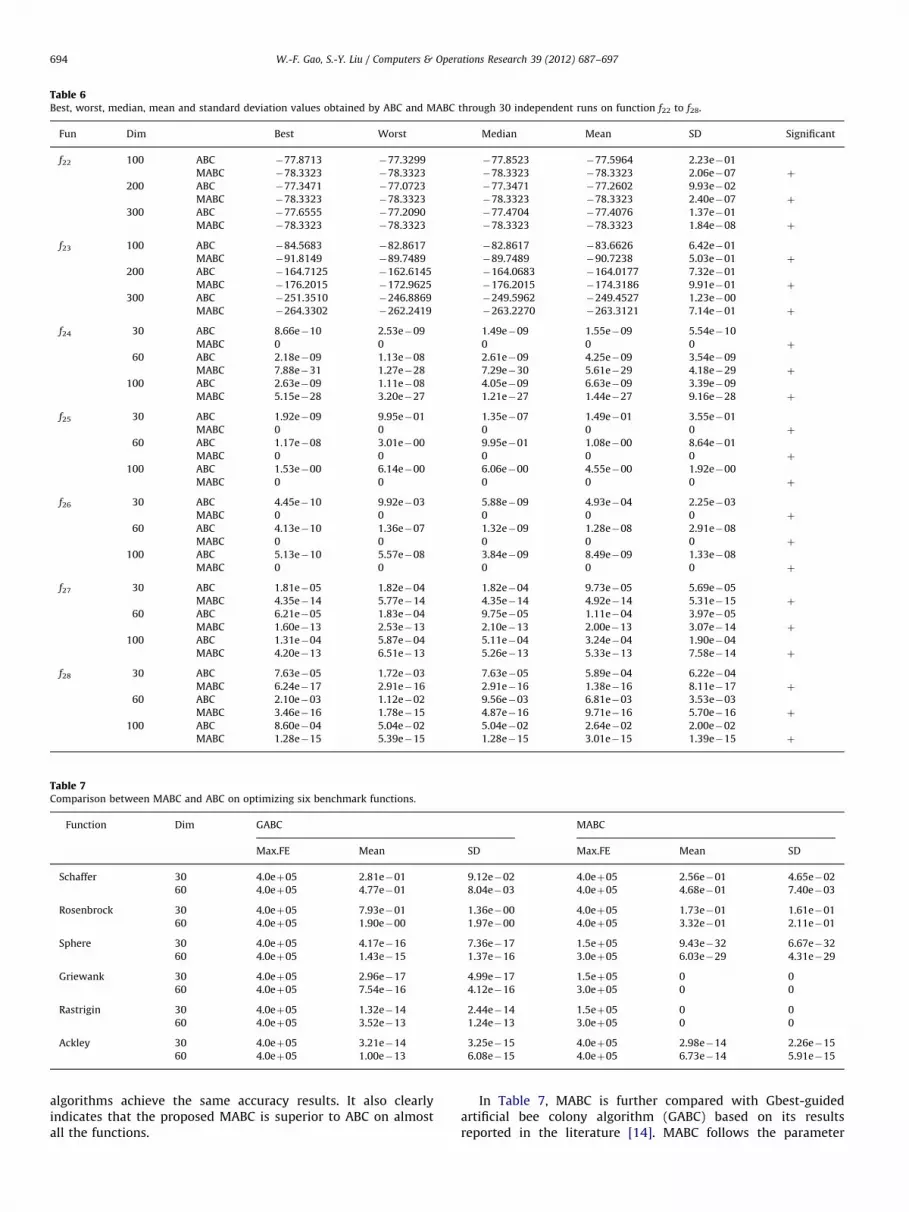
Table 6Best, worst, median, mean and standard deviation values obtained by ABC and MABC through 30 independent runs on function f22 to f28.

Fun Dim Best Worst Median Mean SD Significant

f22 100 ABC �77.8713 �77.3299 �77.8523 �77.5964 2.23e�01

MABC �78.3323 �78.3323 �78.3323 �78.3323 2.06e�07 þ

200 ABC �77.3471 �77.0723 �77.3471 �77.2602 9.93e�02

MABC �78.3323 �78.3323 �78.3323 �78.3323 2.40e�07 þ

300 ABC �77.6555 �77.2090 �77.4704 �77.4076 1.37e�01

MABC �78.3323 �78.3323 �78.3323 �78.3323 1.84e�08 þ

f23 100 ABC �84.5683 �82.8617 �82.8617 �83.6626 6.42e�01

MABC �91.8149 �89.7489 �89.7489 �90.7238 5.03e�01 þ

200 ABC �164.7125 �162.6145 �164.0683 �164.0177 7.32e�01

MABC �176.2015 �172.9625 �176.2015 �174.3186 9.91e�01 þ

300 ABC �251.3510 �246.8869 �249.5962 �249.4527 1.23e�00

MABC �264.3302 �262.2419 �263.2270 �263.3121 7.14e�01 þ

f24 30 ABC 8.66e�10 2.53e�09 1.49e�09 1.55e�09 5.54e�10

MABC 0 0 0 0 0 þ

60 ABC 2.18e�09 1.13e�08 2.61e�09 4.25e�09 3.54e�09

MABC 7.88e�31 1.27e�28 7.29e�30 5.61e�29 4.18e�29 þ

100 ABC 2.63e�09 1.11e�08 4.05e�09 6.63e�09 3.39e�09

MABC 5.15e�28 3.20e�27 1.21e�27 1.44e�27 9.16e�28 þ

f25 30 ABC 1.92e�09 9.95e�01 1.35e�07 1.49e�01 3.55e�01

MABC 0 0 0 0 0 þ

60 ABC 1.17e�08 3.01e�00 9.95e�01 1.08e�00 8.64e�01

MABC 0 0 0 0 0 þ

100 ABC 1.53e�00 6.14e�00 6.06e�00 4.55e�00 1.92e�00

MABC 0 0 0 0 0 þ

f26 30 ABC 4.45e�10 9.92e�03 5.88e�09 4.93e�04 2.25e�03

MABC 0 0 0 0 0 þ

60 ABC 4.13e�10 1.36e�07 1.32e�09 1.28e�08 2.91e�08

MABC 0 0 0 0 0 þ

100 ABC 5.13e�10 5.57e�08 3.84e�09 8.49e�09 1.33e�08

MABC 0 0 0 0 0 þ

f27 30 ABC 1.81e�05 1.82e�04 1.82e�04 9.73e�05 5.69e�05

MABC 4.35e�14 5.77e�14 4.35e�14 4.92e�14 5.31e�15 þ

60 ABC 6.21e�05 1.83e�04 9.75e�05 1.11e�04 3.97e�05

MABC 1.60e�13 2.53e�13 2.10e�13 2.00e�13 3.07e�14 þ

100 ABC 1.31e�04 5.87e�04 5.11e�04 3.24e�04 1.90e�04

MABC 4.20e�13 6.51e�13 5.26e�13 5.33e�13 7.58e�14 þ

f28 30 ABC 7.63e�05 1.72e�03 7.63e�05 5.89e�04 6.22e�04

MABC 6.24e�17 2.91e�16 2.91e�16 1.38e�16 8.11e�17 þ

60 ABC 2.10e�03 1.12e�02 9.56e�03 6.81e�03 3.53e�03

MABC 3.46e�16 1.78e�15 4.87e�16 9.71e�16 5.70e�16 þ

100 ABC 8.60e�04 5.04e�02 5.04e�02 2.64e�02 2.00e�02

MABC 1.28e�15 5.39e�15 1.28e�15 3.01e�15 1.39e�15 þ

Table 7Comparison between MABC and ABC on optimizing six benchmark functions.

Function Dim GABC MABC

Max.FE Mean SD Max.FE Mean SD

Schaffer 30 4.0eþ05 2.81e�01 9.12e�02 4.0eþ05 2.56e�01 4.65e�02

60 4.0eþ05 4.77e�01 8.04e�03 4.0eþ05 4.68e�01 7.40e�03

Rosenbrock 30 4.0eþ05 7.93e�01 1.36e�00 4.0eþ05 1.73e�01 1.61e�01

60 4.0eþ05 1.90e�00 1.97e�00 4.0eþ05 3.32e�01 2.11e�01

Sphere 30 4.0eþ05 4.17e�16 7.36e�17 1.5eþ05 9.43e�32 6.67e�32

60 4.0eþ05 1.43e�15 1.37e�16 3.0eþ05 6.03e�29 4.31e�29

Griewank 30 4.0eþ05 2.96e�17 4.99e�17 1.5eþ05 0 0

60 4.0eþ05 7.54e�16 4.12e�16 3.0eþ05 0 0

Rastrigin 30 4.0eþ05 1.32e�14 2.44e�14 1.5eþ05 0 0

60 4.0eþ05 3.52e�13 1.24e�13 3.0eþ05 0 0

Ackley 30 4.0eþ05 3.21e�14 3.25e�15 4.0eþ05 2.98e�14 2.26e�15

60 4.0eþ05 1.00e�13 6.08e�15 4.0eþ05 6.73e�14 5.91e�15

W.-F. Gao, S.-Y. Liu / Computers & Operations Research 39 (2012) 687–697694

algorithms achieve the same accuracy results. It also clearlyindicates that the proposed MABC is superior to ABC on almostall the functions.

In Table 7, MABC is further compared with Gbest-guidedartificial bee colony algorithm (GABC) based on its resultsreported in the literature [14]. MABC follows the parameter

W.-F. Gao, S.-Y. Liu / Computers & Operations Research 39 (2012) 687–697 695

settings in the original paper of GABC [14]. It is clear that MABCworks better in all cases and achieves better performancethan GABC.

Summarizing the earlier statements, the ability of MABC isthat it can prevent bees from falling into the local minimum,reduce evolution process significantly and more efficiently (con-verges faster), compute with more efficiency, and improve bees’searching abilities for ABC.

0 2 4 6 8 10 12 14 16x 104

10−20

10−15

10−10

10−5

100

105

FE

fitne

ss

f13 function with D = 30

ABCMABC

fitne

ss

0 2 4 6 8 10 12 14 16x 104

0.25

0.3

0.35

0.4

0.45

0.5

FE

fitne

ss

f21 function with D = 30fit

ness

0 0.5 1 1.5 2 2.5 3 3.5

x 105

10−15

10−10

10−5

100

105

FE

fitne

ss

f11 function with D = 60

fitne

ss

0 1 2 3 4 5 6x 105

10−15

10−10

10−5

100

105

FE

fitne

ss

f18 function with D = 100

fitne

ss

ABCMABC

ABCMABC

ABCMABC

Fig. 1. Convergence performance of the diff

4.3. Effects of each modification on the performance of MABC

In order to analyze the modifications respectively, we call thebasic ABC with the proposed initialization as ABC1, and therandom initialization with the proposed search mechanism(i.e., MABC without the proposed initialization) as ABC2. Wecompare the convergence performance of the different ABCs onthe four test functions to see that how much the initialization and

0 2 4 6 8 10 12 14 16x 104

10−15

10−10

10−5

100

105

FE

f20 function with D = 30

0 0.5 1 1.5 2 2.5 3 3.5x 105

10−30

10−25

10−20

10−15

10−10

10−5

100

105

1010

FE

f1 function with D = 60

0 0.5 1 1.5 2 2.5 3 3.5

x 105

10−15

10−10

10−5

100

105

FE

f12 function with D = 60

0 1 2 3 4 5 6x 105

10−30

10−25

10−20

10−15

10−10

10−5

100

105

FE

f19 function with D = 100

ABCMABC

ABCMABC

ABCMABC

ABCMABC

erent ABCs on the eight test functions.

0 2 4 6 8 10 12 14 16x 104

10−35

10−30

10−25

10−20

10−15

10−10

10−5

100

105

FE

fitne

ss

function f1 with D = 30

ABCABC1ABC2MABC

0 2 4 6 8 10 12 14 16x 104FE

0 2 4 6 8 10 12 14 16x 104FE

0 2 4 6 8 10 12 14 16x 104FE

function f3 with D = 30

10−15

10−10

10−5

100

105

fitne

ss

10−35

10−30

10−25

10−20

10−15

10−10

10−5

100

105

fitne

ss

10−2

10−4

10−6

10−8

10−10

10−12

10−14

100

102

fitne

ss

function f11 with D = 30 function f15 with D = 30

ABCABC1ABC2MABC

ABCABC1ABC2MABC

ABCABC1ABC2MABC

Fig. 2. Convergence performance of the different ABCs on the four test functions.

W.-F. Gao, S.-Y. Liu / Computers & Operations Research 39 (2012) 687–697696

the search mechanism make contribution to improving theperformance of the algorithm respectively. The results are pre-sented in Fig. 2. It can be observed that, ABC1 and ABC2 aresuperior to ABC, which implies that both the initialization and thesearch mechanism have positive effect on the performance of thealgorithm. Especially, ABC2 greatly outperforms ABC. On the otherhand, the performance comparisons of ABC2 and MABC are not soapparent as those of ABC1 and MABC, which means that thesearch mechanism plays a pivotal role in the proposed algorithm.However, though the contribution of the initialization is far lessthan the search mechanism, the comparisons of MABC and ABC2,ABC and ABC1 show the initialization is at work.

5. Conclusion

In this paper, we have developed a novel optimization algo-rithm, called MABC, through introducing the modified solutionsearch equation to ABC and proposing a new framework withoutprobabilistic selection scheme and scout bee phase. In addition,the initial population is generated by combining chaotic systemswith opposition-based learning method to enhance the globalconvergence. The experimental results tested on 28 benchmarkfunctions show that MABC outperforms ABC and MABC. As aconsequence, MABC may be a promising and viable tool to dealwith complex numerical optimization problems. It is desirable tofurther apply MABC to solving those more complex real-worldcontinuous optimization problems, such as clustering, datamining, design and optimization of communication networks.The future work includes the studies on how to extend MABC tohandle those combinatorial optimization problems, such as flowshop scheduling problem, vehicle routing problem and travelingsalesman problem.

Acknowledgments

This work is supported by National Nature Science Foundationof China (No. 60974082), Fundamental Research Funds for theCentral Universities (No. JY10000970006, No. K50510700004) andFoundation of State Key Lab. of Integrated Services Networks ofChina.

References

[1] Tang KS, Man KF, Kwong S, He Q. Genetic algorithms and their applications.IEEE Signal Processing Magazine 1996;13:22–37.

[2] Kennedy J, Eberhart R. Particle swarm optimization. In: IEEE internationalconference on neural networks; 1995. p. 1942–8.

[3] Dorigo M, Stutzle T. Ant colony optimization. Cambridge: MA MIT Press;2004.

[4] Simon D. Biogeography-based optimization. IEEE Transaction on EvolutionaryComputation 2008;12:702–13.

[5] Wang DW. Colony location algorithm for assignment problems. Journal ofControl Theory and Applications 2004;2:111–6.

[6] Karaboga D. An idea based on honey bee swarm for numerical optimization.Technical Report-TR06, Kayseri, Turkey: Erciyes University; 2005.

[7] Karaboga D, Basturk B. A powerful and efficient algorithm for numericalfunction optimization: artificial bee colony (ABC) algorithm. Journal of GlobalOptimization 2007;39:171–459.

[8] Karaboga D, Basturk B. On the performance of artificial bee colony (ABC)algorithm. Applied Soft Computing 2008;8:687–97.

[9] Karaboga D, Basturk B. A comparative study of artificial bee colony algorithm.Applied Mathematics and Computation 2009;214:108–32.

[10] Singh A. An artificial bee colony algorithm for the leaf-constrained minimumspanning tree problem. Applied Soft Computing 2009;9:625–31.

[11] Kang F, et al. Structural inverse analysis by hybrid simplex artificial beecolony algorithms. Computers & Structures 2009;87:861–70.

[12] Samrat L, et al. Artificial bee colony algorithm for small signal modelparameter extraction of MESFET. Engineering Applications of ArtificialIntelligence 2010;11:1573–2916.

[13] Storn R, Price K. Differential evolution–A simple and efficient heuristic forglobal optimization over continuous spaces. Journal of Global Optimization2010;23:689–94.

W.-F. Gao, S.-Y. Liu / Computers & Operations Research 39 (2012) 687–697 697

[14] Zhu GP, Kwong S. Gbest-guided artificial bee colony algorithm for numericalfunction optimization. Applied Mathematics and Computation 2010,doi:10.1016/j.amc.2010.08.049.

[15] Akay B, Karaboga D. A modified artificial bee colony algorithm for real-parameter optimization. Information Sciences 2010, doi:10.1016/j.ins.2010.07.015.

[16] Alatas B. Chaotic bee colony algorithms for global numerical optimization.Expert Systems with Applications 2010;37:5682–7.

[17] Rahnamayan S, et al. Opposition-based differential evolution. IEEE Transac-tion on Evolutionary Computation 2008;12:64–79.

[18] Shang YW, Qiu YH. A note on the extended Rosenbrock function. Evolu-tionary Computation 2006;14:119–26.