A Monomial Chaos Approach for Efficient Uncertainty Quantification in Nonlinear Problems

Copyright © by SIAM. Unauthorized reproduction of this article is prohibited.

SIAM J. SCI. COMPUT. c© 2008 Society for Industrial and Applied MathematicsVol. 30, No. 3, pp. 1296–1317

A MONOMIAL CHAOS APPROACH FOR EFFICIENTUNCERTAINTY QUANTIFICATION IN NONLINEAR PROBLEMS∗

JEROEN A. S. WITTEVEEN† AND HESTER BIJL†

Abstract. A monomial chaos approach is presented for efficient uncertainty quantification innonlinear computational problems. Propagating uncertainty through nonlinear equations can becomputationally intensive for existing uncertainty quantification methods. It usually results in a setof nonlinear equations which can be coupled. The proposed monomial chaos approach employs apolynomial chaos expansion with monomials as basis functions. The expansion coefficients are solvedfor using differentiation of the governing equations, instead of a Galerkin projection. This results in adecoupled set of linear equations even for problems involving polynomial nonlinearities. This reducesthe computational work per additional polynomial chaos order to the equivalence of a single Newtoniteration. Error estimates are derived, and monomial chaos is applied to uncertainty quantification ofthe Burgers equation and a two-dimensional boundary layer flow problem. The results are comparedwith results of the Monte Carlo method, the perturbation method, the Galerkin polynomial chaosmethod, and a nonintrusive polynomial chaos method.

Key words. uncertainty quantification, polynomial chaos, computational fluid dynamics, nondeterministic approaches

AMS subject classifications. 65C20, 65C30, 65N30

DOI. 10.1137/06067287X

1. Introduction. In practical computational problems, physical parameters andboundary conditions are often subject to uncertainty. Until recently, these physicaluncertainties were usually neglected, which resulted in a single deterministic run forthe mean values of the uncertain parameters. Nowadays, such a deterministic simu-lation is no longer adequate for reliable computational predictions. Therefore, therehas recently been a growing interest in accounting for physical uncertainties in com-putational problems [4].

Modeling uncertainty has been common in computational structure mechanicsfor some time now [15]. Uncertainty analysis in computational fluid dynamics is rel-atively new [12, 19, 24]. An important characteristic of problems in fluid dynamics isthat they are governed by a system of nonlinear partial differential equations. Thediscretization of these equations for realistic flows results in computational problemsinvolving millions of unknowns. This makes deterministic computational fluid dynam-ics already computationally intensive. Therefore, it is important to apply uncertaintyquantification methods which can deal with the nonlinearities in an efficient way.By developing efficient methods, uncertainty quantification can become economicallyfeasible in practical flow problems.

Physical problems are usually described mathematically in terms of differentialequations. The uncertainty in these problems can often be modeled by parametricuncertainties. Therefore, parametric uncertainty is considered in a physical model

∗Received by the editors October 20, 2006; accepted for publication (in revised form) November29, 2007; published electronically March 21, 2008. This research is supported by the TechnologyFoundation STW, applied science division of NWO, and the technology programme of the Ministryof Economic Affairs.

http://www.siam.org/journals/sisc/30-3/67287.html†Department of Aerospace Engineering, Delft University of Technology, Kluyverweg 1, 2629 HS

Delft, The Netherlands ([email protected], [email protected]).

1296


A MONOMIAL CHAOS APPROACH 1297

described by the following differential equation for u(x, t, ω) with operator L andsource term S:

(1.1) L(x, t, α(ω);u(x, t, ω)) = S(x, t, α(ω)), x ∈ D, t ∈ [0, T ],

with appropriate initial and boundary conditions and α(ω) an uncertain parameterwith a known uncertainty distribution. The argument ω is used to emphasize the factthat an uncertain variable is a function of the random event ω ∈ Ω of the probabilityspace (Ω, σ, P ). Equation (1.1) is an uncertainty quantification problem for the uncer-tain variable u(x, t, ω). Below, four widely used uncertainty quantification methodsare briefly reviewed for comparison with the proposed monomial chaos approach: theMonte Carlo method, the perturbation method [10], the Galerkin polynomial chaosmethod [3], and a nonintrusive polynomial chaos method [9]. For simplicity, themethods are reviewed for the case of a single uncertain parameter α(ω). They allhave extensions to higher dimensions.

The Monte Carlo method. A robust approach to solving (1.1) is the Monte Carlomethod. It is based on solving the deterministic problem multiple times for a set ofN realizations of the uncertain parameter {αk}Nk=1 with αk ≡ α(ωk),

(1.2) L(x, t, αk;uk(x, t)) = S(x, t, αk), k = 1, . . . , N,

with uk(x, t) ≡ u(x, t, ωk). The stochastic properties of the output can be obtainedfrom the set of N realizations of the uncertain variable {uk(x, t)}Nk=1. Due to the slowconvergence rate, the standard Monte Carlo approach can be impractical when solvinga single deterministic problem already involving a large amount of computationalwork. Methods exist to improve the convergence rate of standard Monte Carlo, suchas Latin-hypercube sampling and variance reduction techniques; see, for example, [6].

The perturbation method. A fast method for determining low-order statistics isthe perturbation method (also called the moment method) [7, 10, 16]. It has recentlybeen applied to problems in computational fluid dynamics [12, 17]. In the perturbationmethod the statistical moments of the output are expanded around the expectedvalue of the uncertain parameter using Taylor series expansions. These expansionsare usually truncated at second order, since for higher orders the equations becomeextremely complicated [3, 10]. The second-order estimate of the mean value is givenby [10] as

(1.3) E[u(x, t, ω)] ≈ u(x, t, ω)

∣∣∣∣α=μα

+1

2Var(α(ω))

∂2u

∂α2

∣∣∣∣α=μα

,

with μα ≡ E[α(ω)]. For the first-order approximation, this relation reduces toE[u(x, t, ω)] ≈ u(x, t, ω)|μα . The first-order estimate of the variance is given as

(1.4) Var[u(x, t, ω)] ≈(∂u

∂α

∣∣∣∣α=μα

)2

Var[α(ω)].

The moment approximations require the computation of the first and second sensitiv-ity derivatives of the solution u(x, t, ω) with respect to the uncertain parameter α(ω)for α(ω) = μα. A method for evaluating these sensitivity derivatives is the continuoussensitivity equation method [7, 16]. In the continuous sensitivity equation method a

differential equation for the ith sensitivity derivative ∂iu∂αi |μα

is obtained by implicit


1298 JEROEN A. S. WITTEVEEN AND HESTER BIJL

differentiation of the governing equation (1.1) with respect to α for α(ω) = μα. Theresulting equation is called the ith continuous sensitivity equation

(1.5)∂i

∂αiL(x, t, α(ω);u(x, t, ω))

∣∣∣∣μα

=∂i

∂αiS(x, t, α(ω))

∣∣∣∣μα

.

The application of the perturbation method is limited to low-order approximationsfor small perturbations, i.e., inputs with a small variance. Furthermore, the methodcannot readily be extended to compute the probability distribution function of theresponse process [3, 10].

The Galerkin polynomial chaos method. A method that is not limited to low-order statistics and small perturbations is the polynomial chaos expansion introducedby Ghanem and Spanos [3]. The method has recently been applied to computationalfluid dynamics [19, 24]. The polynomial chaos expansion is a polynomial expansionof orthogonal polynomials in terms of random variables to approximate the uncer-tainty distribution of the output. The method is based on the homogeneous chaostheory of Wiener [21]. The homogeneous polynomial chaos expansion, which is basedon Hermite polynomials and Gaussian random variables, can approximate any func-tional in L2(C) and converges in the L2(C) sense [2]. It can achieve an exponentialconvergence rate for Gaussian input distributions due to the orthogonality of the Her-mite polynomials with respect to the Gaussian measure. The exponential convergencehas been extended to other input distributions by employing other basis polynomials[20, 22, 23]. The expansion coefficients are determined in the context of a stochas-tic finite element approach by using a Galerkin projection in probability space. Thepolynomial chaos expansions of the uncertain input parameter α(ω) and the uncertainsolution u(x, t, ω) are

(1.6) α(ω) =1∑

j=0

αjΦj(ξ(ω)), u(x, t, ω) =

∞∑i=0

ui(x, t)Φi(ξ(ω)),

where {Φi(ξ)}∞i=0 is a set of orthogonal polynomials and the random variable ξ(ω)is given by a linear transformation of α(ω) to an appropriate standard domain, i.e.[−1, 1], [0,∞), or (−∞,∞). Due to this linear transformation the polynomial chaosexpansion of α(ω) in (1.6) is exact within the first two terms. For the numericalimplementation the polynomial chaos expansion for u(x, t, ω) in (1.6) is truncated to(p+1) terms, where p is the polynomial chaos order of the approximation. Substitutingthe truncated expansions into (1.1) and performing a Galerkin projection onto eachpolynomial basis {Φi(ξ)}pi=0 results in a coupled set of (p+1) deterministic equations

(1.7)

⟨L

⎛⎝x, t,

1∑j=0

αjΦj ;

p∑i=0

uiΦi

⎞⎠ ,Φk

⟩=

⟨S

⎛⎝x, t,

1∑j=0

αjΦj

⎞⎠ ,Φk

⟩

for k = 0, 1, . . . , p. This system of equations can be solved using standard iterativemethods [5]. The Galerkin polynomial chaos method can be intrusive to implementand computationally intensive to solve, due to the coupled set of equations (1.7).

A nonintrusive polynomial chaos method. To avoid solving a coupled set ofequations, a nonintrusive polynomial chaos method can be used. It approximatesthe polynomial chaos coefficients by solving a series of deterministic problems. Anexample of a nonintrusive polynomial chaos method is the method of Hosder and



Walters (see [9, 18]). The polynomial chaos expansion coefficients {uk(x, t)}pk=0

in (1.6) are approximated by evaluating the deterministic problem at (p + 1) pointsin random space {ξk}pk=0, with ξk ≡ ξ(ωk),

(1.8) L(x, t, αk;u∗k(x, t)) = S(x, t, αk), k = 0, 1, . . . , p,

where u∗k(x, t) is the realization of u(x, t, ω) for α(ω) = αk. The polynomial chaos co-

efficients {uk(x, t)}pk=0 are then approximated by the following relatively small linearsystem:

(1.9)

⎛⎜⎜⎜⎜⎝

Φ0(ξ0) Φ1(ξ0) · · · Φp(ξ0)

Φ0(ξ1) Φ1(ξ1) · · · Φp(ξ1)

......

. . ....

Φ0(ξp) Φ1(ξp) · · · Φp(ξp)

⎞⎟⎟⎟⎟⎠

⎛⎜⎜⎜⎜⎝

u0(x, t)

u1(x, t)

...

up(x, t)

⎞⎟⎟⎟⎟⎠ =

⎛⎜⎜⎜⎜⎝

u∗0(x, t)

u∗1(x, t)

...

u∗p(x, t)

⎞⎟⎟⎟⎟⎠ ,

which can be solved using a single LU decomposition. This nonintrusive polynomialchaos method can be shown to converge to the Galerkin polynomial chaos expansioncoefficients under certain conditions [9]. As for the Monte Carlo method (1.2), non-intrusive polynomial chaos results in a set of equations (1.8) which coincide with thedeterministic problem for varying parameter values. However, the number of deter-ministic evaluations can be orders of magnitude smaller than for a standard MonteCarlo simulation due to the combination with the polynomial chaos expansion.

Compared to solving the problem deterministically, using a nonintrusive poly-nomial chaos method results in a multiplication of computational work by a factor(p + 1). For computationally very intensive problems this increase of computationalwork can be a major drawback for the application of uncertainty quantification. Con-sider, for example, practical applications of nonlinear computational fluid dynamicsin time dependent problems involving complex geometries. These deterministic prob-lems can already take weeks or even longer to solve. An increase of this amount ofcomputational work by a factor (p + 1) is significant. Especially in iterative designprocesses of industrial applications this can make uncertainty quantification imprac-tical. On the other hand, uncertainty quantification is in these cases essential forrobust design optimization. Therefore, there is a need for a further reduction of thecomputational costs of uncertainty quantification methods.

In this paper, a monomial chaos approach is proposed to reduce the costs of uncer-tainty quantification in computationally intensive nonlinear problems. The methodemploys the polynomial chaos expansion with monomials as basis functions. Themonomial chaos expansion coefficients are solved for using differentiation of the gov-erning equations, instead of a Galerkin projection. This results in a decoupled set oflinear equations even for problems involving polynomial nonlinearities. This reducesthe computational work per additional polynomial chaos order to the equivalence of asingle Newton iteration. Therefore, monomial chaos can be a computationally efficientalternative for existing uncertainty quantification methods in nonlinear problems. Themonomial chaos approach is introduced in this paper for one uncertain input param-eter to demonstrate the properties of the method and to make a basic comparisonwith other uncertainty quantification methods. The extension of monomial chaos tomultiple uncertain parameters and random fields is briefly addressed.

The paper is organized as follows. The monomial chaos is introduced and er-ror estimates derived in section 2. In section 3 the monomial chaos is applied to



the Burgers equation to demonstrate the properties of the proposed approach for astandard nonlinear advection-diffusion test problem in one dimension. The resultsare compared with results of the perturbation method, the Galerkin polynomial chaosmethod, and the nonintrusive polynomial chaos method in section 4. In section 5 themonomial chaos is applied to a two-dimensional boundary layer flow problem as anexample of a standard nonlinear test problem from two-dimensional incompressiblefluid dynamics. In section 6 the conclusions are summarized.

2. The monomial chaos approach. In this section the monomial chaos ap-proach is proposed. In section 2.1 the monomial chaos approach is introduced ingeneral as applied to (1.1). Error estimates are given in section 2.2.

2.1. The monomial chaos formulation. The monomial chaos approach em-ploys a polynomial chaos expansion with monomials as basis functions to determinethe uncertainty distribution of the output. The equations for the monomial chaosexpansion coefficients are obtained by differentiating the deterministic equation withrespect to the uncertain input parameter. This results in a decoupled set of (p + 1)equations for the (p + 1) coefficients of a pth-order monomial chaos expansion, inwhich each equation solves for a monomial chaos coefficient sequentially. Due to theproduct rule the differentiation of the governing equations also results in a set oflinear equations even for problems involving polynomial nonlinearities. This reducesthe additional computational work per polynomial chaos order to the equivalence ofa single Newton iteration. Therefore, monomial chaos can be an efficient alternativefor uncertainty quantification in computationally intensive nonlinear problems.

Consider the application of monomial chaos to a physical model involving poly-nomial nonlinearities and parametric uncertainty given by (1.1),

L(x, t, α(ω);u(x, t, ω)) = S(x, t, α(ω)).

The uncertain parameter α(ω) and the solution u(x, t, ω) are expanded into a poly-nomial chaos expansion

(2.1) α(ω) =1∑

j=0

αjΨj(ξ(ω)), u(x, t, ω) =

∞∑i=0

ui(x, t)Ψi(ξ(ω)),

where the random variable ξ(ω) is given by a linear transformation of the uncertaininput parameter α(ω) to an appropriate standard domain, i.e., [−1, 1], [0,∞), or(−∞,∞) [23]. Due to this linear transformation the polynomial chaos expansion ofα(ω) in (2.1) is exact within the first two terms. In the monomial chaos the basispolynomials {Ψi(ξ)}∞i=0 are monomials around ξ(ω) = μξ with μξ ≡ E[ξ(ω)]:

(2.2) Ψi(ξ(ω)) = (ξ(ω) − μξ)i, i = 0, 1, . . . .

These monomials are chosen as basis functions because they satisfy the property

(2.3)djΨi

dξj

∣∣∣∣ξ=μξ

=

{i!, i = j,

0, i �= j,

which says that taking the jth derivative of the monomials {Ψi(ξ)}∞i=0 with respect toξ at ξ(ω) = μξ results in a nonzero term for i = j only. This property of monomialsresults in the decoupled set of equations for the monomial chaos coefficients {ui(x, t)}.



Substitution of the monomial chaos expansions (2.1) with (2.2) into the governingequation (1.1) results in

(2.4) L

⎛⎝x, t,

1∑j=0

αjΨj(ξ);

∞∑i=0

ui(x, t)Ψi(ξ)

⎞⎠ = S

⎛⎝x, t,

1∑j=0

αjΨj(ξ)

⎞⎠ .

To obtain a set of equations for the expansion coefficients of the solution {ui(x, t)},(2.4) is differentiated with respect to ξ for ξ(ω) = μξ. Taking the kth derivativeof (2.4) results in an equation for the kth expansion coefficient uk(x, t),

∂k

∂ξkL

⎛⎝x, t,

1∑j=0

αjΨj(ξ);

∞∑i=0

ui(x, t)Ψi(ξ)

⎞⎠

∣∣∣∣∣ξ=μξ

=∂k

∂ξkS

⎛⎝x, t,

1∑j=0

αjΨj(ξ)

⎞⎠

∣∣∣∣∣ξ=μξ

(2.5)

for k = 0, 1, . . . . This set of equations can be discretized using standard discretizationtechniques [8]. Due to the combination of differentiation of (2.4) and property (2.3),all higher-order coefficients {ui(x, t)}∞i=k+1 drop out of the equation, which results in a

decoupled set of equations for uk(x, t) in terms of {ui(x, t)}k−1i=0 . This is illustrated in

section 3 where the monomial chaos is applied to the Burgers equation. Furthermore,the decoupled set of equations (2.5) is linear in uk(x, t) due to the product rule indifferentiation, even if the governing equation (1.1) contains polynomial nonlinearities(except for k = 0). The equation for k = 0 coincides with the deterministic problemfor the expected value of the uncertain parameter μα. For nonlinear problems solvedusing Newton linearization, the additional computational work per polynomial chaosorder is proportional to one Newton iteration.

A pth-order monomial chaos approximation of the solution u(x, t, ω) is given bytruncating the monomial chaos expansion for u(x, t, ω) in (2.1) at p. The monomialchaos coefficients {αj}1

j=0 of the uncertain parameter α(ω) with a known uncertaintydistribution can be determined by differentiating the monomial chaos expansion forα(ω) in (2.1) with respect to ξ for ξ(ω) = μξ, which results, using property (2.3), in

(2.6) αj =1

j!

djα

dξj

∣∣∣∣ξ=μξ

, j = 0, 1,

where djαdξj |μξ

is known and α0 = μα.

Equations (2.5) are similar to the continuous sensitivity equations (1.5) of theperturbation method, which are obtained by implicit differentiation. The monomialchaos method can be viewed as an extension of the perturbation method, which is usu-ally limited to second-order approximations of the first two moments. The monomialchaos approach can be employed for obtaining higher-order approximations of theuncertainty distribution and the statistical moments of the output at computationalcosts equivalent to those of the perturbation method.

On the other hand, in the monomial chaos approach the uncertain parameter andvariables are expanded in a polynomial expansion as in the polynomial chaos method,using monomials instead of orthogonal polynomials in the polynomial chaos method.

https://www.researchgate.net/publication/258225325_Numerical_Computation_of_Internal_and_External_Flow-Vol_I?el=1_x_8&enrichId=rgreq-92f4b1e28b6b056f003e1b384522a6eb-XXX&enrichSource=Y292ZXJQYWdlOzIyMDQxMjE3NTtBUzoxMDMxNDI1MjM5MzI2ODFAMTQwMTYwMjUwMjU2Nw==



The monomial chaos approach can therefore be applied to the same set of arbitraryinput probability distributions as the polynomial chaos method. The outputs of themonomial chaos approach are higher-order approximations of the distribution andthe statistical moments by solving a decoupled set of linear equations, instead of apossibly coupled set of nonlinear equations in the polynomial chaos method.

Next to the relatively low computational work per polynomial chaos order themonomial chaos has additional advantages which are important for practical appli-cations. First, the polynomial chaos order of the monomial chaos approximation canbe determined during the computation while solving for the higher-order coefficientssequentially. Second, the equations (2.5) depend only on the mean value of the un-certain input parameter μα. Therefore, the influence of different input uncertaintydistributions and variances can be studied after solving (2.5) once. This is an im-portant property since in practical problems the input distribution itself can also besubject to uncertainty.

The monomial chaos is moderately intrusive, since for solving (2.5) the summationof the matrix and vector entries in the deterministic solver have to be modified. Fordecreasing the intrusiveness of the monomial chaos, the differentiation of the governingequations can be replaced by finite difference differentiation in random space.

Here, the monomial chaos approach is considered for a single uncertain input pa-rameter. The monomial chaos approach can be extended to multiple uncertain inputparameters by introducing a vector of random variables ξ(ω) = (ξ1(ω), . . . , ξn(ω)),where n is the number of uncertain input parameters. The basis consists in thatcase of multidimensional monomials Ψi(ξ(ω)), which are tensor products of the one-dimensional monomials Ψi(ξj(ω)). The set of equations for the monomial chaoscoefficients (2.5) is then derived using mixed partial derivatives of (2.4) with respectto the random variables {ξj(ω)}nj=0.

The uncertainty quantification methods reviewed in section 1 can also be extendedto multiple uncertain input parameters. For comparison, in the extension of theperturbation method to multiple uncertain input parameters, the statistical momentsof the output are expanded around the expected value of the uncertain parametersusing multidimensional Taylor series expansions. The polynomial chaos method canbe extended to n uncertain parameters by using a multidimensional polynomial chaosexpansion in (1.6). The multidimensional polynomial chaos expansion is based on avector of random variables ξ(ω) = (ξ1(ω), . . . , ξn(ω)) and multidimensional orthogonalpolynomials Φi(ξ(ω)).

A random field can be handled by the monomial chaos method by first represent-ing the random field in terms of a finite number of independent random input pa-rameters using a Karhunen–Loeve expansion [11] as in the polynomial chaos method.For a random field with a relatively high spatial correlation, the number of randominput parameters needed to reach a reasonable accuracy with the Karhunen–Loeveexpansion can be small. In that case the monomial chaos method can be applied tothe random input parameters to resolve the effect of the random field. For randomfields and random processes with low correlation the required number of random in-put parameters can be much higher, and approaches other than the monomial chaosmethod or the polynomial chaos method can be more competitive.

2.2. Error estimates. In this section error estimates for the monomial chaosapproach are derived. For simplicity the arguments x and t are dropped. Aftercomputing the monomial chaos coefficients in (2.5), approximations of the mean μu,variance σ2

u, higher-order moments, and the distribution function can be derived. If



the uncertain variable u(ω) is expanded in an infinite monomial chaos series, the meanμu is given in terms of the monomial chaos coefficients {ui}∞i=0 by

(2.7) μu =

∞∑i=0

uiμξ,i,

with μξ,i the ith central statistical moment of ξ(ω),

(2.8) μξ,i =

∫supp(ξ)

Ψi(ξ)pξ(ξ)dξ,

with μξ,0 = 1, μξ,1 = 0 and where supp(ξ) and pξ(ξ) are the support and the proba-bility density of ξ(ω), respectively. The variance σ2

u is given by

(2.9) σ2u =

∞∑i=0

∞∑j=0

uiujμξ,i+j ,

with

(2.10) ui =

{ui − μu, i = 0,

ui, i = 1, 2, . . . .

In the numerical implementation the infinite series in (2.7) and (2.9) are truncated ata polynomial chaos order p. The errors in the approximation in the mean εμu

and thevariance εσ2

udue to the truncation of the monomial chaos expansion are then given

by

(2.11) εμu = −∞∑

i=p+1

uiμξ,i,

and

(2.12) εσ2u

= −2

∞∑i=p+1

∞∑j=p+1

uiujμξ,i+j .

If the monomial chaos coefficients ui decrease fast enough with i for i = p+1, p+2, . . . ,such that the leading truncation error term is due to neglecting the (p+1)th coefficient,then the truncation errors can be estimated as

(2.13) εμu ≈ −up+1μξ,p+1

and

(2.14) εσ2u≈ −2u2

p+1μ2ξ,p+1,

which says that the leading error term in the approximation of the variance σ2u results

in an underestimation. These a posteriori error estimates can be used in a stop-ping criterion for determining the polynomial chaos order p of the monomial chaosapproximation.

Another contribution to the error in the mean μu and the variance σ2u can be due

to the divergence of the monomial chaos expansion in a part of the domain of ξ(ω). In



case of an input distribution with an infinite support, i.e., ξ(ω) ∈ (−∞,∞), there isalways a domain ξ(ω) ∈ (−∞, ξ−]∪ [ξ+,∞) in which the monomial chaos expansion ofu(ω), (2.1), diverges. However, it is demonstrated in the following propositions thatthe divergence of the monomial chaos expansion in ξ(ω) ∈ (−∞, ξ−]∪ [ξ+,∞) resultsin errors εμu , εσ2

uwhich are in general small with respect to the truncation errors εμu

and εσ2u, and the mean μu and variance σ2

u.Proposition 2.1. Let ξ(ω) ∈ (−∞,∞) and let ξ(ω) ∈ (ξ−, ξ+) be the domain of

convergence of the monomial chaos expansion of u(ω), (2.1). If the probability densitypξ(ξ) of ξ(ω) decreases fast enough as ξ → ±∞ such that

(2.15)

∞∑i=0

|ui|∣∣∣∣∣∫

(−∞,ξ−]∪[ξ+,∞)

Ψi(ξ)pξ(ξ)dξ

∣∣∣∣∣ ∣∣∣∣∣∣

∞∑i=p+1

ui

∫ ξ+

ξ−Ψi(ξ)pξ(ξ)dξ

∣∣∣∣∣∣ ,then the error in the monomial chaos approximation of the mean μu due to the di-vergence of the monomial chaos expansion in ξ(ω) ∈ (−∞, ξ−] ∪ [ξ+,∞) is smallcompared to the truncation error; i.e., |εμu | |εμu |.

Proof. The error εμuin the monomial chaos approximation of the mean μu due

to the divergence in ξ(ω) ∈ (−∞, ξ−] ∪ [ξ+,∞) is defined as

(2.16) εμu=

∞∑i=0

ui

∫(−∞,ξ−]∪[ξ+,∞)

Ψi(ξ)pξ(ξ)dξ,

with

(2.17)∣∣∣∣∣∞∑i=0

ui

∫(−∞,ξ−]∪[ξ+,∞)

Ψi(ξ)pξ(ξ)dξ

∣∣∣∣∣ ≤∞∑i=0

|ui|∣∣∣∣∣∫

(−∞,ξ−]∪[ξ+,∞)

Ψi(ξ)pξ(ξ)dξ

∣∣∣∣∣ .The truncation error εμu

in the monomial chaos approximation of the mean μu dueto the truncation of the monomial chaos expansion at p is given by (2.11),

εμu = −∞∑

i=p+1

ui

∫ ∞

−∞Ψi(ξ)pξ(ξ)dξ(2.18)

= −∞∑

i=p+1

ui

∫(−∞,ξ−]∪[ξ+,∞)

Ψi(ξ)pξ(ξ)dξ −∞∑

i=p+1

ui

∫ ξ+

ξ−Ψi(ξ)pξ(ξ)dξ,

with

(2.19)∣∣∣∣∣∣∞∑

i=p+1

ui

∫(−∞,ξ−]∪[ξ+,∞)

Ψi(ξ)pξ(ξ)dξ

∣∣∣∣∣∣ ≤∞∑i=0

|ui|∣∣∣∣∣∫

(−∞,ξ−]∪[ξ+,∞)

Ψi(ξ)pξ(ξ)dξ

∣∣∣∣∣ .According to the assumption, |εμu | |εμu |.

Proposition 2.2. Let ξ(ω) ∈ (−∞,∞), and let ξ(ω) ∈ (ξ−, ξ+) be the domainof convergence of the monomial chaos expansion of u(ω), (2.1). If (i) the probabilitydensity pξ(ξ) of ξ(ω) decreases fast enough as ξ → ±∞ such that

(2.20)

∣∣∣∣∣∞∑i=0

ui

∫(−∞,ξ−]∪[ξ+,∞)

Ψi(ξ)pξ(ξ)dξ

∣∣∣∣∣ ∣∣∣∣∣∞∑i=0

ui

∫ ξ+

ξ−Ψi(ξ)pξ(ξ)dξ

∣∣∣∣∣ ,



or (ii) the probability density pξ(ξ) of ξ(ω) decreases fast enough as ξ → ±∞ such that(2.15) holds and the probability density pξ(ξ)of ξ(ω) decreases fast enough as ξ → ±∞such that

(2.21)

∣∣∣∣∣∣∞∑

i=p+1

ui

∫ ∞

−∞Ψi(ξ)pξ(ξ)dξ

∣∣∣∣∣∣ ∣∣∣∣∣

p∑i=0

ui

∫ ∞

−∞Ψi(ξ)pξ(ξ)dξ

∣∣∣∣∣ ,then |εμu

| |μu|.Proof. The error εμu

in the monomial chaos approximation of the mean μu dueto the divergence in ξ(ω) ∈ (−∞, ξ−] ∪ [ξ+,∞) is given by (2.16),

εμu =

∞∑i=0

ui

∫(−∞,ξ−]∪[ξ+,∞)

Ψi(ξ)pξ(ξ)dξ.

The mean μu is given by (2.7) and (2.8), which can be written as

(2.22) μu =

∞∑i=0

ui

∫(−∞,ξ−]∪[ξ+,∞)

Ψi(ξ)pξ(ξ)dξ +

∞∑i=0

ui

∫ ξ+

ξ−Ψi(ξ)pξ(ξ)dξ.

According to assumption (i), |εμu | |μu|. The mean μu based on an infinite monomialchaos series expansion of u(ω) is given by (2.7) and (2.8), which can also be writtenas

(2.23) μu =

p∑i=0

ui

∫ ∞

−∞Ψi(ξ)pξ(ξ)dξ +

∞∑i=p+1

ui

∫ ∞

−∞Ψi(ξ)pξ(ξ)dξ.

The error εμu in the monomial chaos approximation of the mean μu due to the trun-cation of the monomial chaos expansion at p is given by (2.11),

(2.24) εμu= −

∞∑i=p+1

ui

∫ ∞

−∞Ψi(ξ)pξ(ξ)dξ.

According to assumption (ii), we have |εμu | |μu|. The result of Proposition 2.1gives |εμu

| |μu|.An example of a probability distribution that can satisfy the assumptions of

Propositions 2.1 and 2.2 is the Gaussian distribution with density function pξ(ξ) =

(1/√

2πσ2ξ )exp(−(ξ − μξ)

2/(2σ2ξ )), and μξ and σ2

ξ the mean and variance of ξ(ω),

respectively. This probability density function is exponentially decreasing as ξ → ±∞.Whether a given Gaussian probability distribution satisfies the assumptions dependson the combination of a not too large variance of the uncertain input parameterthrough σ2

ξ and sufficient regularity of the uncertain variable u(ω) through {ui}∞i=0,

ξ−, and ξ+. One can use (2.15), (2.20), and (2.21) to verify whether the monomialchaos expansion of a certain order p is appropriate to use in a particular application.Similar propositions hold for the variance σ2

u and the errors εσ2u

and εσ2u.

3. Application of monomial chaos. In this section the monomial chaos isapplied to the Burgers equation. The test problem is intended for demonstratingthe properties of monomial chaos applied to a nonlinear problem and for comparingthe results to those of other methods. The Burgers equation is often used to study



0 0.2 0.4 0.6 0.8 10

0.2

0.4

0.6

0.8

1

ν=0→

←ν=0.25

←ν=0.5←ν=1ν=2→

ν=∞→

sensor location x=0.5→

position x

velo

city

u

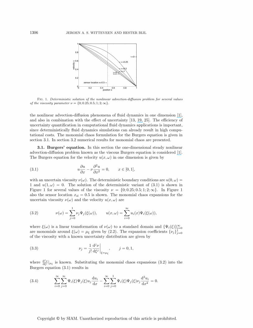
Fig. 1. Deterministic solution of the nonlinear advection-diffusion problem for several valuesof the viscosity parameter ν = {0; 0.25; 0.5; 1; 2;∞}.

the nonlinear advection-diffusion phenomena of fluid dynamics in one dimension [1],and also in combination with the effect of uncertainty [13, 19, 25]. The efficiency ofuncertainty quantification in computational fluid dynamics applications is important,since deterministically fluid dynamics simulations can already result in high compu-tational costs. The monomial chaos formulation for the Burgers equation is given insection 3.1. In section 3.2 numerical results for monomial chaos are presented.

3.1. Burgers’ equation. In this section the one-dimensional steady nonlinearadvection-diffusion problem known as the viscous Burgers equation is considered [1].The Burgers equation for the velocity u(x, ω) in one dimension is given by

(3.1) u∂u

∂x− ν

∂2u

∂x2= 0, x ∈ [0, 1],

with an uncertain viscosity ν(ω). The deterministic boundary conditions are u(0, ω) =1 and u(1, ω) = 0. The solution of the deterministic variant of (3.1) is shown inFigure 1 for several values of the viscosity ν = {0; 0.25; 0.5; 1; 2;∞}. In Figure 1also the sensor location xsl = 0.5 is shown. The monomial chaos expansions for theuncertain viscosity ν(ω) and the velocity u(x, ω) are

(3.2) ν(ω) =1∑

j=0

νjΨj(ξ(ω)), u(x, ω) =

∞∑i=0

ui(x)Ψi(ξ(ω)),

where ξ(ω) is a linear transformation of ν(ω) to a standard domain and {Ψi(ξ)}∞i=0

are monomials around ξ(ω) = μξ given by (2.2). The expansion coefficients {νj}1j=0

of the viscosity with a known uncertainty distribution are given by

(3.3) νj =1

j!

djν

dξj

∣∣∣∣ξ=μξ

, j = 0, 1,

where djνdξj |μξ

is known. Substituting the monomial chaos expansions (3.2) into the

Burgers equation (3.1) results in

(3.4)

∞∑i=0

∞∑j=0

Ψi(ξ)Ψj(ξ)ujdui

dx−

∞∑i=0

1∑j=0

Ψi(ξ)Ψj(ξ)νjd2ui

dx2= 0.

https://www.researchgate.net/publication/37425937_Computation_Fluid_Mechanics_and_Heat_Transfer?el=1_x_8&enrichId=rgreq-92f4b1e28b6b056f003e1b384522a6eb-XXX&enrichSource=Y292ZXJQYWdlOzIyMDQxMjE3NTtBUzoxMDMxNDI1MjM5MzI2ODFAMTQwMTYwMjUwMjU2Nw==


https://www.researchgate.net/publication/235082312_Uncertainty_Analysis_for_Fluid_Mechanics_with_Applications?el=1_x_8&enrichId=rgreq-92f4b1e28b6b056f003e1b384522a6eb-XXX&enrichSource=Y292ZXJQYWdlOzIyMDQxMjE3NTtBUzoxMDMxNDI1MjM5MzI2ODFAMTQwMTYwMjUwMjU2Nw==



Taking the kth derivative of (3.4) with respect to ξ for ξ(ω) = μξ and using theLeibniz identity and property (2.3) results in a differential equation for uk(x),

(3.5)

k∑l=0

(k

l

)uk−l(x)

dul

dx−

k∑l=max{0,k−1}

(k

l

)νk−l

d2ul

dx2= 0, k = 0, 1, . . . .

Terms without uk(x) can be brought to the right-hand side of (3.5), which results in

u0du0

dx− ν0

d2u0

dx2= 0, k = 0,(3.6a)

ukdu0

dx+ u0

duk

dx− ν0

d2uk

dx2= −

k−1∑l=1

(k

l

)uk−l(x)

dul

dx+ kν1

d2uk−1

dx2, k = 1, 2, . . . .

(3.6b)

As mentioned before, the equation for k = 0, (3.6a), coincides with the deterministicproblem for the mean value of the uncertain viscosity ν0. Equations (3.6b) form adecoupled set of equations for the higher-order monomial chaos coefficients uk(x),with k = 1, 2, . . . , as function of {uj(x)}k−1

j=0 which can be solved sequentially forincreasing k. These equations are linear in uk(x). The computational work for solv-ing each equation of (3.6b) is equivalent to one Newton iteration for solving (3.6a).Therefore, monomial chaos results in relatively low computational costs per additionalpolynomial chaos order compared to the deterministic solve.

A pth-order approximation of the solution for u(x, ω) can be obtained by trun-cating the monomial expansion for u(x, ω) in (3.2) at p. The error estimates (2.13)and (2.14) can be used to determine a suitable polynomial chaos order p of the ap-proximation. Equations (2.7) and (2.9) can be used to determine the approximationof the mean and the variance of the velocity u(x, ω).

3.2. Results for Burgers’ equation. In this section results of the monomialchaos for the Burgers equation are presented. In section 4, the results of the monomialchaos approach are compared to results of the perturbation method, the Galerkinpolynomial chaos method, and a nonintrusive polynomial chaos method as reviewedin section 1. For this comparison two error measures are used for the error in themean εμu(x) and the variance εσ2

u(x) at the sensor location xsl = 0.5:

(3.7) εμu =

∣∣∣∣μu(xsl) − μu,ref(xsl)

μu,ref(xsl)

∣∣∣∣ , εσ2u

=

∣∣∣∣∣σ2u(xsl) − σ2

u,ref(xsl)

σ2u,ref(xsl)

∣∣∣∣∣ .The reference solution is a Monte Carlo simulation based on 106 realizations of theuncertain parameter ν(ω) evenly spaced in sample space ω ∈ [0, 1]. Approximationsof the probability distribution function and the probability density function are alsopresented. A second-order finite volume method is used to discretize the spatial do-main. The nonlinear problem is solved using Newton linearization with an appropriateconvergence criterion εnl = 10−9 for the L∞-norm of the residual, which results forthis problem in four Newton iterations.

The mean value of the uncertain input is assumed to be μν = 1. Probabilitydistributions with either a finite or a (semi-)infinite support of the uncertain viscosityν(ω) are considered. The uniform distribution is chosen for the distribution on thefinite domain. This corresponds to the assumption of an interval uncertainty, which




0 0.2 0.4 0.6 0.8 10

0.2

0.4

0.6

0.8

1

postition x

velo

city

u

p=7

meanuncertainty bars

(a) mean and uncertainty bars

0.52 0.54 0.56 0.58 0.6 0.62 0.64 0.66

0

0.2

0.4

0.6

0.8

1

velocity u

prob

abili

ty d

istr

ibut

ion

func

tion

exactMCh p=7MCh p=3

(b) distribution function at xsl

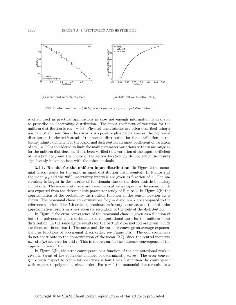
Fig. 2. Monomial chaos (MCh) results for the uniform input distribution.

is often used in practical applications in case not enough information is availableto prescribe an uncertainty distribution. The input coefficient of variation for theuniform distribution is covν = 0.3. Physical uncertainties are often described using anormal distribution. Since the viscosity is a positive physical parameter, the lognormaldistribution is selected instead of the normal distribution for the distribution on the(semi-)infinite domain. For the lognormal distribution an input coefficient of variationof covν = 0.2 is considered to limit the main parameter variations to the same range asfor the uniform distribution. It has been verified that variation of the input coefficientof variation covν and the choice of the sensor location xsl do not affect the resultssignificantly in comparison with the other methods.

3.2.1. Results for the uniform input distribution. In Figure 2 the mono-mial chaos results for the uniform input distribution are presented. In Figure 2(a)the mean μu and the 90% uncertainty intervals are given as function of x. The un-certainty is largest in the interior of the domain due to the deterministic boundaryconditions. The uncertainty bars are asymmetrical with respect to the mean, whichwas expected from the deterministic parameter study of Figure 1. In Figure 2(b) theapproximation of the probability distribution function at the sensor location xsl isshown. The monomial chaos approximations for p = 3 and p = 7 are compared to thereference solution. The 7th-order approximation is very accurate, and the 3rd-orderapproximation results in a less accurate resolution of the tails of the distribution.

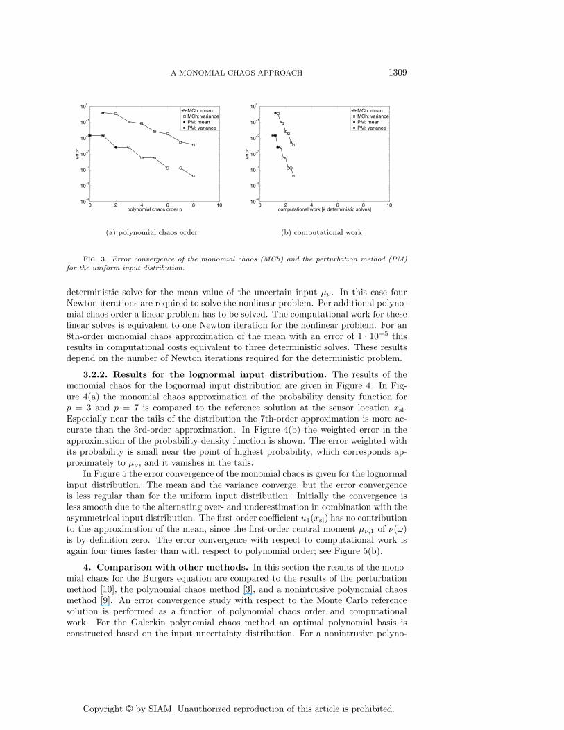
In Figure 3 the error convergence of the monomial chaos is given as a function ofboth the polynomial chaos order and the computational work for the uniform inputdistribution. In the same figure results for the perturbation method are given, whichare discussed in section 4. The mean and the variance converge on average exponen-tially as functions of polynomial chaos order; see Figure 3(a). The odd coefficientsdo not contribute to the approximation of the mean (2.7), since the central momentsμν,i of ν(ω) are zero for odd i. This is the reason for the staircase convergence of theapproximation of the mean.

In Figure 3(b), the error convergence as a function of the computational work isgiven in terms of the equivalent number of deterministic solves. The error conver-gence with respect to computational work is four times faster than the convergencewith respect to polynomial chaos order. For p = 0 the monomial chaos results in a



0 2 4 6 8 1010

−6

10−5

10−4

10−3

10−2

10−1

100

polynomial chaos order p

erro

r

MCh: meanMCh: variancePM: meanPM: variance

(a) polynomial chaos order

0 2 4 6 8 1010

−6

10−5

10−4

10−3

10−2

10−1

100

computational work [# deterministic solves]

erro

r


(b) computational work

Fig. 3. Error convergence of the monomial chaos (MCh) and the perturbation method (PM)for the uniform input distribution.

deterministic solve for the mean value of the uncertain input μν . In this case fourNewton iterations are required to solve the nonlinear problem. Per additional polyno-mial chaos order a linear problem has to be solved. The computational work for theselinear solves is equivalent to one Newton iteration for the nonlinear problem. For an8th-order monomial chaos approximation of the mean with an error of 1 · 10−5 thisresults in computational costs equivalent to three deterministic solves. These resultsdepend on the number of Newton iterations required for the deterministic problem.

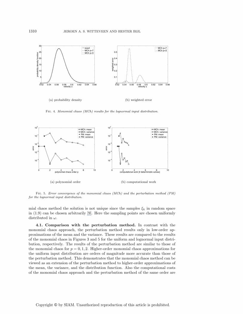
3.2.2. Results for the lognormal input distribution. The results of themonomial chaos for the lognormal input distribution are given in Figure 4. In Fig-ure 4(a) the monomial chaos approximation of the probability density function forp = 3 and p = 7 is compared to the reference solution at the sensor location xsl.Especially near the tails of the distribution the 7th-order approximation is more ac-curate than the 3rd-order approximation. In Figure 4(b) the weighted error in theapproximation of the probability density function is shown. The error weighted withits probability is small near the point of highest probability, which corresponds ap-proximately to μν , and it vanishes in the tails.

In Figure 5 the error convergence of the monomial chaos is given for the lognormalinput distribution. The mean and the variance converge, but the error convergenceis less regular than for the uniform input distribution. Initially the convergence isless smooth due to the alternating over- and underestimation in combination with theasymmetrical input distribution. The first-order coefficient u1(xsl) has no contributionto the approximation of the mean, since the first-order central moment μν,1 of ν(ω)is by definition zero. The error convergence with respect to computational work isagain four times faster than with respect to polynomial order; see Figure 5(b).

4. Comparison with other methods. In this section the results of the mono-mial chaos for the Burgers equation are compared to the results of the perturbationmethod [10], the polynomial chaos method [3], and a nonintrusive polynomial chaosmethod [9]. An error convergence study with respect to the Monte Carlo referencesolution is performed as a function of polynomial chaos order and computationalwork. For the Galerkin polynomial chaos method an optimal polynomial basis isconstructed based on the input uncertainty distribution. For a nonintrusive polyno-

https://www.researchgate.net/publication/267778567_A_Non-Intrusive_Polynomial_Chaos_Method_For_Uncertainty_Propagation_in_CFD_Simulations?el=1_x_8&enrichId=rgreq-92f4b1e28b6b056f003e1b384522a6eb-XXX&enrichSource=Y292ZXJQYWdlOzIyMDQxMjE3NTtBUzoxMDMxNDI1MjM5MzI2ODFAMTQwMTYwMjUwMjU2Nw==

https://www.researchgate.net/publication/230872901_Stochastic_Finite_Elements?el=1_x_8&enrichId=rgreq-92f4b1e28b6b056f003e1b384522a6eb-XXX&enrichSource=Y292ZXJQYWdlOzIyMDQxMjE3NTtBUzoxMDMxNDI1MjM5MzI2ODFAMTQwMTYwMjUwMjU2Nw==



0.52 0.54 0.56 0.58 0.6 0.62 0.64 0.660

5

10

15

20

25

30

velocity u

prob

abili

ty d

ensi

ty fu

nctio

n

exactMCh p=7MCh p=3

(a) probability density

0.52 0.54 0.56 0.58 0.6 0.62 0.64 0.660

0.1

0.2

0.3

0.4

0.5

velocity u

wei

ghte

d er

ror

MCh p=7MCh p=3

(b) weighted error

Fig. 4. Monomial chaos (MCh) results for the lognormal input distribution.

0 2 4 6 8 10

10−4

10−3

10−2

10−1

100


erro

r


(a) polynomial order

0 2 4 6 8 10

10−4

10−3

10−2

10−1

100


erro

r



Fig. 5. Error convergence of the monomial chaos (MCh) and the perturbation method (PM)for the lognormal input distribution.

mial chaos method the solution is not unique since the samples ξk in random spacein (1.9) can be chosen arbitrarily [9]. Here the sampling points are chosen uniformlydistributed in ω.

4.1. Comparison with the perturbation method. In contrast with themonomial chaos approach, the perturbation method results only in low-order ap-proximations of the mean and the variance. These results are compared to the resultsof the monomial chaos in Figures 3 and 5 for the uniform and lognormal input distri-bution, respectively. The results of the perturbation method are similar to those ofthe monomial chaos for p = 0, 1, 2. Higher-order monomial chaos approximations forthe uniform input distribution are orders of magnitude more accurate than those ofthe perturbation method. This demonstrates that the monomial chaos method can beviewed as an extension of the perturbation method to higher-order approximations ofthe mean, the variance, and the distribution function. Also the computational costsof the monomial chaos approach and the perturbation method of the same order are




0 2 4 6 8 1010

−6

10−4

10−2

100


erro

r

MCh: meanMCh: variancePC: meanPC: variance


0 2 4 6 8 10 1210

−6

10−4

10−2

100


erro

r



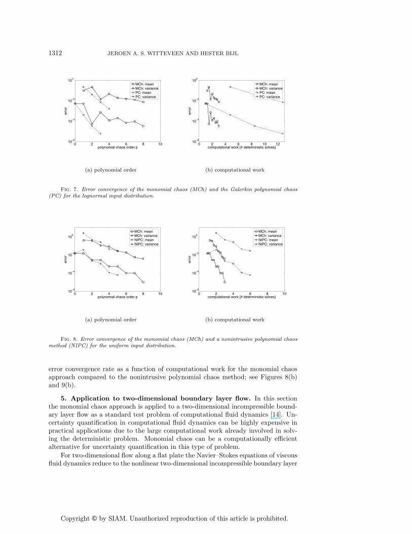
Fig. 6. Error convergence of the monomial chaos (MCh) and the Galerkin polynomial chaos(PC) for the uniform input distribution.

similar; see Figures 3(b) and 5(b). For higher-order approximations the monomialchaos approach maintains these low computational costs per additional polynomialchaos order.

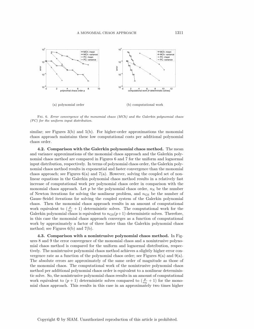
4.2. Comparison with the Galerkin polynomial chaos method. The meanand variance approximations of the monomial chaos approach and the Galerkin poly-nomial chaos method are compared in Figures 6 and 7 for the uniform and lognormalinput distribution, respectively. In terms of polynomial chaos order, the Galerkin poly-nomial chaos method results in exponential and faster convergence than the monomialchaos approach; see Figures 6(a) and 7(a). However, solving the coupled set of non-linear equations in the Galerkin polynomial chaos method results in a relatively fastincrease of computational work per polynomial chaos order in comparison with themonomial chaos approach. Let p be the polynomial chaos order, nN be the numberof Newton iterations for solving the nonlinear problem, and nGS be the number ofGauss–Seidel iterations for solving the coupled system of the Galerkin polynomialchaos. Then the monomial chaos approach results in an amount of computationalwork equivalent to ( p

nN+ 1) deterministic solves. The computational work for the

Galerkin polynomial chaos is equivalent to nGS(p+1) deterministic solves. Therefore,in this case the monomial chaos approach converges as a function of computationalwork by approximately a factor of three faster than the Galerkin polynomial chaosmethod; see Figures 6(b) and 7(b).

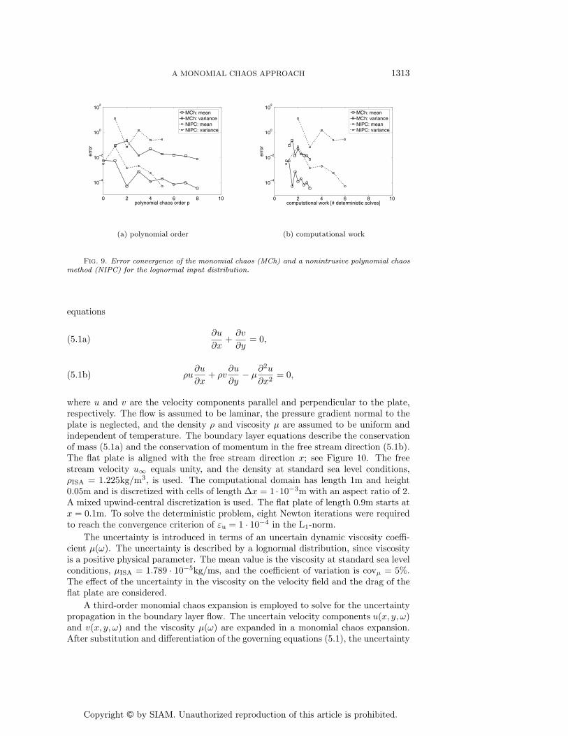
4.3. Comparison with a nonintrusive polynomial chaos method. In Fig-ures 8 and 9 the error convergence of the monomial chaos and a nonintrusive polyno-mial chaos method is compared for the uniform and lognormal distribution, respec-tively. The nonintrusive polynomial chaos method achieves a slightly higher error con-vergence rate as a function of the polynomial chaos order; see Figures 8(a) and 9(a).The absolute errors are approximately of the same order of magnitude as those ofthe monomial chaos. The computational work of the nonintrusive polynomial chaosmethod per additional polynomial chaos order is equivalent to a nonlinear determinis-tic solve. So, the nonintrusive polynomial chaos results in an amount of computationalwork equivalent to (p + 1) deterministic solves compared to ( p

nN+ 1) for the mono-

mial chaos approach. This results in this case in an approximately two times higher



0 2 4 6 8 1010

−6

10−4

10−2

100


erro

r



0 2 4 6 8 10 1210

−6

10−4

10−2

100


erro

r



Fig. 7. Error convergence of the monomial chaos (MCh) and the Galerkin polynomial chaos(PC) for the lognormal input distribution.

0 2 4 6 8 1010

−6

10−4

10−2

100


erro

r

MCh: meanMCh: varianceNIPC: meanNIPC: variance


0 2 4 6 8 1010

−6

10−4

10−2

100


erro

r



Fig. 8. Error convergence of the monomial chaos (MCh) and a nonintrusive polynomial chaosmethod (NIPC) for the uniform input distribution.

error convergence rate as a function of computational work for the monomial chaosapproach compared to the nonintrusive polynomial chaos method; see Figures 8(b)and 9(b).

5. Application to two-dimensional boundary layer flow. In this sectionthe monomial chaos approach is applied to a two-dimensional incompressible bound-ary layer flow as a standard test problem of computational fluid dynamics [14]. Un-certainty quantification in computational fluid dynamics can be highly expensive inpractical applications due to the large computational work already involved in solv-ing the deterministic problem. Monomial chaos can be a computationally efficientalternative for uncertainty quantification in this type of problem.

For two-dimensional flow along a flat plate the Navier–Stokes equations of viscousfluid dynamics reduce to the nonlinear two-dimensional incompressible boundary layer

https://www.researchgate.net/publication/51997480_Boundary-Layer_Theory?el=1_x_8&enrichId=rgreq-92f4b1e28b6b056f003e1b384522a6eb-XXX&enrichSource=Y292ZXJQYWdlOzIyMDQxMjE3NTtBUzoxMDMxNDI1MjM5MzI2ODFAMTQwMTYwMjUwMjU2Nw==



0 2 4 6 8 10

10−4

10−2

100

102


erro

r



0 2 4 6 8 10

10−4

10−2

100

102


erro

r



Fig. 9. Error convergence of the monomial chaos (MCh) and a nonintrusive polynomial chaosmethod (NIPC) for the lognormal input distribution.

equations

∂u

∂x+

∂v

∂y= 0,(5.1a)

ρu∂u

∂x+ ρv

∂u

∂y− μ

∂2u

∂x2= 0,(5.1b)

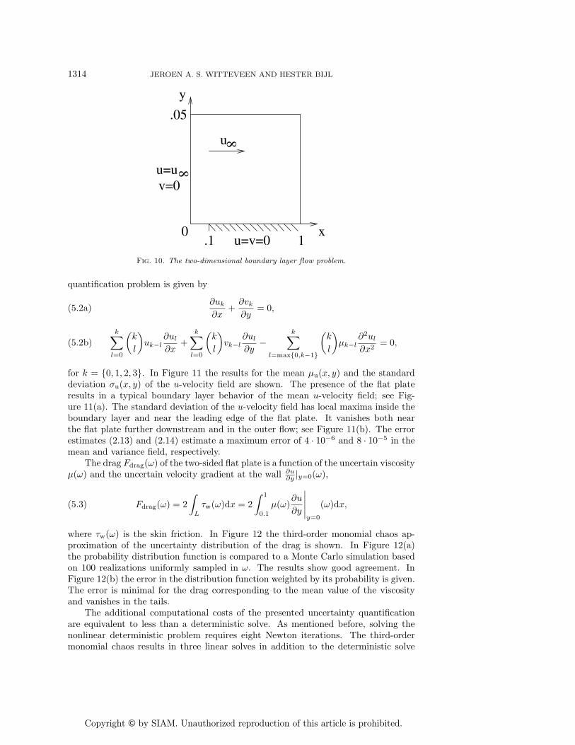
where u and v are the velocity components parallel and perpendicular to the plate,respectively. The flow is assumed to be laminar, the pressure gradient normal to theplate is neglected, and the density ρ and viscosity μ are assumed to be uniform andindependent of temperature. The boundary layer equations describe the conservationof mass (5.1a) and the conservation of momentum in the free stream direction (5.1b).The flat plate is aligned with the free stream direction x; see Figure 10. The freestream velocity u∞ equals unity, and the density at standard sea level conditions,ρISA = 1.225kg/m3, is used. The computational domain has length 1m and height0.05m and is discretized with cells of length Δx = 1 ·10−3m with an aspect ratio of 2.A mixed upwind-central discretization is used. The flat plate of length 0.9m starts atx = 0.1m. To solve the deterministic problem, eight Newton iterations were requiredto reach the convergence criterion of εu = 1 · 10−4 in the L1-norm.

The uncertainty is introduced in terms of an uncertain dynamic viscosity coeffi-cient μ(ω). The uncertainty is described by a lognormal distribution, since viscosityis a positive physical parameter. The mean value is the viscosity at standard sea levelconditions, μISA = 1.789 · 10−5kg/ms, and the coefficient of variation is covμ = 5%.The effect of the uncertainty in the viscosity on the velocity field and the drag of theflat plate are considered.

A third-order monomial chaos expansion is employed to solve for the uncertaintypropagation in the boundary layer flow. The uncertain velocity components u(x, y, ω)and v(x, y, ω) and the viscosity μ(ω) are expanded in a monomial chaos expansion.After substitution and differentiation of the governing equations (5.1), the uncertainty



x

y

.05

.10

u

u=v=0

8

8u=uv=0

1Fig. 10. The two-dimensional boundary layer flow problem.

quantification problem is given by

∂uk

∂x+

∂vk∂y

= 0,(5.2a)

k∑l=0

(k

l

)uk−l

∂ul

∂x+

k∑l=0

(k

l

)vk−l

∂ul

∂y−

k∑l=max{0,k−1}

(k

l

)μk−l

∂2ul

∂x2= 0,(5.2b)

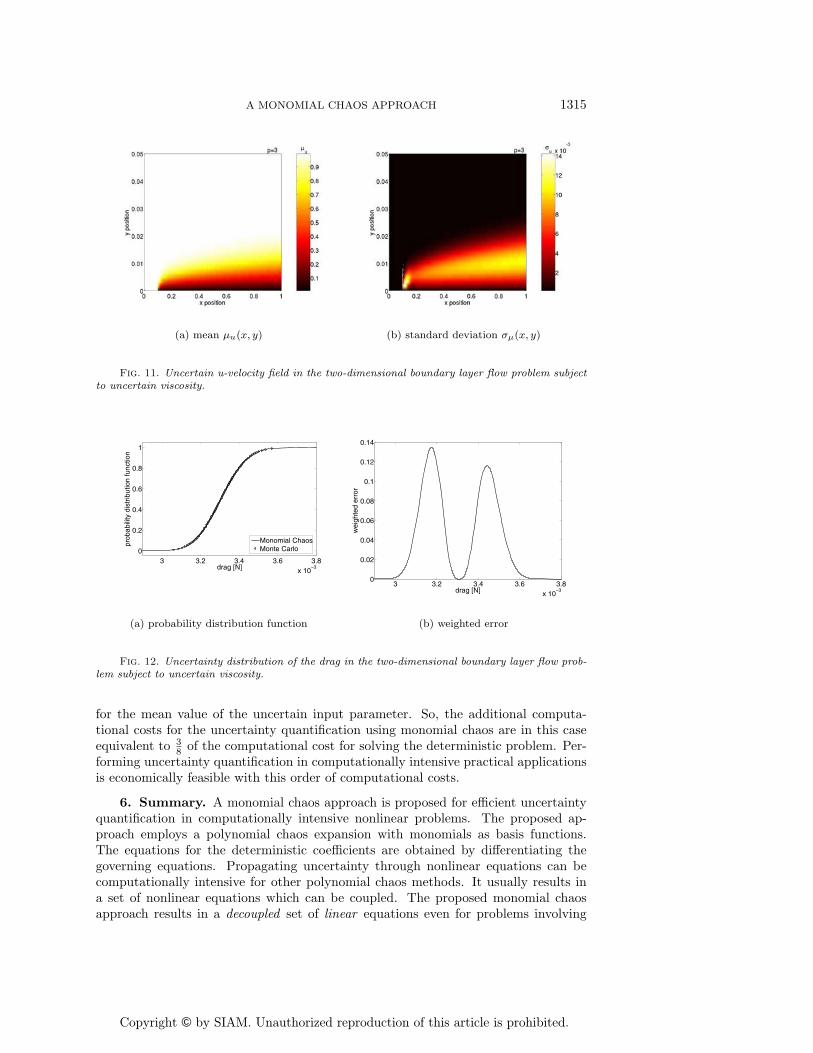
for k = {0, 1, 2, 3}. In Figure 11 the results for the mean μu(x, y) and the standarddeviation σu(x, y) of the u-velocity field are shown. The presence of the flat plateresults in a typical boundary layer behavior of the mean u-velocity field; see Fig-ure 11(a). The standard deviation of the u-velocity field has local maxima inside theboundary layer and near the leading edge of the flat plate. It vanishes both nearthe flat plate further downstream and in the outer flow; see Figure 11(b). The errorestimates (2.13) and (2.14) estimate a maximum error of 4 · 10−6 and 8 · 10−5 in themean and variance field, respectively.

The drag Fdrag(ω) of the two-sided flat plate is a function of the uncertain viscosityμ(ω) and the uncertain velocity gradient at the wall ∂u

∂y |y=0(ω),

(5.3) Fdrag(ω) = 2

∫L

τw(ω)dx = 2

∫ 1

0.1

μ(ω)∂u

∂y

∣∣∣∣∣y=0

(ω)dx,

where τw(ω) is the skin friction. In Figure 12 the third-order monomial chaos ap-proximation of the uncertainty distribution of the drag is shown. In Figure 12(a)the probability distribution function is compared to a Monte Carlo simulation basedon 100 realizations uniformly sampled in ω. The results show good agreement. InFigure 12(b) the error in the distribution function weighted by its probability is given.The error is minimal for the drag corresponding to the mean value of the viscosityand vanishes in the tails.

The additional computational costs of the presented uncertainty quantificationare equivalent to less than a deterministic solve. As mentioned before, solving thenonlinear deterministic problem requires eight Newton iterations. The third-ordermonomial chaos results in three linear solves in addition to the deterministic solve



(a) mean μu(x, y) (b) standard deviation σμ(x, y)

Fig. 11. Uncertain u-velocity field in the two-dimensional boundary layer flow problem subjectto uncertain viscosity.

3 3.2 3.4 3.6 3.8x 10

−3

0

0.2

0.4

0.6

0.8

1

drag [N]

prob

abili

ty d

istr

ibut

ion

func

tion

Monomial ChaosMonte Carlo

(a) probability distribution function

3 3.2 3.4 3.6 3.8x 10

−3

0

0.02

0.04

0.06

0.08

0.1

0.12

0.14

drag [N]

wei

ghte

d er

ror

(b) weighted error

Fig. 12. Uncertainty distribution of the drag in the two-dimensional boundary layer flow prob-lem subject to uncertain viscosity.

for the mean value of the uncertain input parameter. So, the additional computa-tional costs for the uncertainty quantification using monomial chaos are in this caseequivalent to 3

8 of the computational cost for solving the deterministic problem. Per-forming uncertainty quantification in computationally intensive practical applicationsis economically feasible with this order of computational costs.

6. Summary. A monomial chaos approach is proposed for efficient uncertaintyquantification in computationally intensive nonlinear problems. The proposed ap-proach employs a polynomial chaos expansion with monomials as basis functions.The equations for the deterministic coefficients are obtained by differentiating thegoverning equations. Propagating uncertainty through nonlinear equations can becomputationally intensive for other polynomial chaos methods. It usually results ina set of nonlinear equations which can be coupled. The proposed monomial chaosapproach results in a decoupled set of linear equations even for problems involving



polynomial nonlinearities. This reduces the computational work per additional poly-nomial chaos order to the equivalence of a single Newton iteration. Error estimatesfor the monomial chaos approach have been presented. It has been demonstratednumerically that the monomial chaos approach can achieve a 2–3 times faster con-vergence as a function of computational work than other polynomial chaos methods.Application to a two-dimensional flow problem demonstrated that the additional com-putational work for performing an uncertainty quantification using monomial chaoscan be smaller than a single deterministic solve.

REFERENCES

[1] D. A. Anderson, J. C. Tannehill, and R. H. Pletcher, Computational Fluid Mechanicsand Heat Transfer, Ser. Comput. Methods Mech. Thermal Sci., McGraw–Hill, New York,1997.

[2] R. H. Cameron and W. T. Martin, The orthogonal development of nonlinear functionals inseries of Fourier-Hermite functionals, Ann. Math., 48 (1947), pp. 385–392.

[3] R. G. Ghanem and P. Spanos, Stochastic Finite Elements: A Spectral Approach, Springer-Verlag, New York, 1991.

[4] R. G. Ghanem and S. F. Wojtkiewicz, eds., Special issue on uncertainty quantification,SIAM J. Sci. Comput., 26 (2004), issue 2.

[5] A. Greenbaum, Iterative Methods for Solving Linear Systems, SIAM, Philadelphia, 1997.[6] J. M. Hammersley and D. C. Handscomb, Monte Carlo Methods, Methuen’s Monographs on

Applied Probability and Statistics, Fletcher & Son, Norwich, CT, 1964.[7] E. J. Haug, K. Choi, and V. Komkov, Design Sensitivity Analysis of Structural Systems,

Academic Press, Orlando, FL, 1986.[8] C. Hirsch, Numerical Computation of Internal and External Flows, Vol. 1: Fundamentals of

Numerical Discretization, Wiley, Chichester, UK, 1988.[9] S. Hosder, R. W. Walters, and R. Perez, A non-intrusive polynomial chaos method for

uncertainty propagation in CFD simulations, in Proceedings of the 44th AIAA AerospaceSciences Meeting and Exhibit, Reno, NV, 2006, AIAA-2006-891.

[10] M. Kleiber and T. D. Hien, The Stochastic Finite Element Method, John Wiley and Sons,New York, 1992.

[11] M. Loeve, Probability Theory, 4th ed., Springer-Verlag, New York, 1977.

[12] J.-N. Mahieu, S. Etienne, D. Pelletier, and J. Borggaard, A second-order sensitivityequation method for laminar flow, Int. J. Comput. Fluid D, 19 (2005), pp. 143–157.

[13] L. Mathelin and O. P. Le Maitre, A posteriori error analysis for stochastic finite elementsolutions of fluid flows with parametric uncertainties, in Proceedings of the EuropeanConference on Computational Fluid Dynamics (ECCOMAS CFD 2006), Egmond aan Zee,The Netherlands, P. Wesseling, E. Onate, and J. Periaux, eds., TU Delft, The Netherlands,2006.

[14] H. T. Schlichting and K. Gersten, Boundary-Layer Theory, Springer, Berlin, 2000.[15] G. I. Schueller, ed., A state-of-the-art report on computational stochastic mechanics, Prob.

Engrg. Mech., 12 (1997), pp. 197–321.[16] L. G. Stanley and D. L. Stewart, Design Sensitivity Analysis: Computational Issues of

Sensitivity Equation Methods, Frontiers Appl. Math. 25, SIAM, Philadelphia, 2002.[17] E Turgeon, D. Pelletier, and J. Borggaard, A general continuous sensitivity equation

formulation for complex flows, Numer. Heat Transfer B, 42 (2002), pp. 485–408.[18] R. W. Walters, Towards stochastic fluid mechanics via polynomial chaos—Invited, in Pro-

ceedings of the 41st AIAA Aerospace Sciences Meeting and Exhibit, Reno, NV, 2003,AIAA-2003-0413.

[19] R. W. Walters and L. Huyse, Uncertainty Analysis for Fluid Mechanics with Applications,NASA research report NASA/CR-2002-21149, NASA Langley Research Center, Hampton,VA, 2002; available online from http://historical.ncstrl.org/tr/pdf/icase/TR-2002-1.pdf.

[20] X. Wan and G. E. Karniadakis, Beyond Wiener-Askey expansions: Handling arbitrary PDFs,J. Sci. Comput., 27 (2006), pp. 455–464.

[21] N. Wiener, The homogeneous chaos, Amer. J. Math., 60 (1938), pp. 897–936.[22] J. A. S. Witteveen and H. Bijl, Modeling arbitrary uncertainties using Gram-Schmidt poly-

nomial chaos, in Proceedings of the 44th AIAA Aerospace Sciences Meeting and Exhibit,Reno, NV, 2006, AIAA-2006-896.




https://www.researchgate.net/publication/245185869_A_State-of-the-Art_Report_on_Computational_Stochastic_Mechanics?el=1_x_8&enrichId=rgreq-92f4b1e28b6b056f003e1b384522a6eb-XXX&enrichSource=Y292ZXJQYWdlOzIyMDQxMjE3NTtBUzoxMDMxNDI1MjM5MzI2ODFAMTQwMTYwMjUwMjU2Nw==

https://www.researchgate.net/publication/245185869_A_State-of-the-Art_Report_on_Computational_Stochastic_Mechanics?el=1_x_8&enrichId=rgreq-92f4b1e28b6b056f003e1b384522a6eb-XXX&enrichSource=Y292ZXJQYWdlOzIyMDQxMjE3NTtBUzoxMDMxNDI1MjM5MzI2ODFAMTQwMTYwMjUwMjU2Nw==

https://www.researchgate.net/publication/51997480_Boundary-Layer_Theory?el=1_x_8&enrichId=rgreq-92f4b1e28b6b056f003e1b384522a6eb-XXX&enrichSource=Y292ZXJQYWdlOzIyMDQxMjE3NTtBUzoxMDMxNDI1MjM5MzI2ODFAMTQwMTYwMjUwMjU2Nw==

https://www.researchgate.net/publication/268563792_Modeling_Arbitrary_Uncertainties_Using_Gram-Schmidt_Polynomial_Chaos?el=1_x_8&enrichId=rgreq-92f4b1e28b6b056f003e1b384522a6eb-XXX&enrichSource=Y292ZXJQYWdlOzIyMDQxMjE3NTtBUzoxMDMxNDI1MjM5MzI2ODFAMTQwMTYwMjUwMjU2Nw==



https://www.researchgate.net/publication/266732113_Towards_Stochastic_Fluid_Mechanics_via_Polynomial_Chaos?el=1_x_8&enrichId=rgreq-92f4b1e28b6b056f003e1b384522a6eb-XXX&enrichSource=Y292ZXJQYWdlOzIyMDQxMjE3NTtBUzoxMDMxNDI1MjM5MzI2ODFAMTQwMTYwMjUwMjU2Nw==









https://www.researchgate.net/publication/44507349_Iterative_methods_for_solving_linear_systems?el=1_x_8&enrichId=rgreq-92f4b1e28b6b056f003e1b384522a6eb-XXX&enrichSource=Y292ZXJQYWdlOzIyMDQxMjE3NTtBUzoxMDMxNDI1MjM5MzI2ODFAMTQwMTYwMjUwMjU2Nw==

https://www.researchgate.net/publication/220411960_Special_Issue_on_Uncertainty_Quantification?el=1_x_8&enrichId=rgreq-92f4b1e28b6b056f003e1b384522a6eb-XXX&enrichSource=Y292ZXJQYWdlOzIyMDQxMjE3NTtBUzoxMDMxNDI1MjM5MzI2ODFAMTQwMTYwMjUwMjU2Nw==

https://www.researchgate.net/publication/220411960_Special_Issue_on_Uncertainty_Quantification?el=1_x_8&enrichId=rgreq-92f4b1e28b6b056f003e1b384522a6eb-XXX&enrichSource=Y292ZXJQYWdlOzIyMDQxMjE3NTtBUzoxMDMxNDI1MjM5MzI2ODFAMTQwMTYwMjUwMjU2Nw==

https://www.researchgate.net/publication/220395581_Beyond_Wiener-Askey_Expansions_Handling_Arbitrary_PDFs?el=1_x_8&enrichId=rgreq-92f4b1e28b6b056f003e1b384522a6eb-XXX&enrichSource=Y292ZXJQYWdlOzIyMDQxMjE3NTtBUzoxMDMxNDI1MjM5MzI2ODFAMTQwMTYwMjUwMjU2Nw==

https://www.researchgate.net/publication/220395581_Beyond_Wiener-Askey_Expansions_Handling_Arbitrary_PDFs?el=1_x_8&enrichId=rgreq-92f4b1e28b6b056f003e1b384522a6eb-XXX&enrichSource=Y292ZXJQYWdlOzIyMDQxMjE3NTtBUzoxMDMxNDI1MjM5MzI2ODFAMTQwMTYwMjUwMjU2Nw==

https://www.researchgate.net/publication/230872719_The_Orthogonal_Development_of_Non-Linear_Functionals_in_Series_of_Fourier-Hermite_Functionals?el=1_x_8&enrichId=rgreq-92f4b1e28b6b056f003e1b384522a6eb-XXX&enrichSource=Y292ZXJQYWdlOzIyMDQxMjE3NTtBUzoxMDMxNDI1MjM5MzI2ODFAMTQwMTYwMjUwMjU2Nw==

https://www.researchgate.net/publication/230872719_The_Orthogonal_Development_of_Non-Linear_Functionals_in_Series_of_Fourier-Hermite_Functionals?el=1_x_8&enrichId=rgreq-92f4b1e28b6b056f003e1b384522a6eb-XXX&enrichSource=Y292ZXJQYWdlOzIyMDQxMjE3NTtBUzoxMDMxNDI1MjM5MzI2ODFAMTQwMTYwMjUwMjU2Nw==



https://www.researchgate.net/publication/282714892_The_Homogeneous_Chaos?el=1_x_8&enrichId=rgreq-92f4b1e28b6b056f003e1b384522a6eb-XXX&enrichSource=Y292ZXJQYWdlOzIyMDQxMjE3NTtBUzoxMDMxNDI1MjM5MzI2ODFAMTQwMTYwMjUwMjU2Nw==





[23] D. Xiu and G. E. Karniadakis, The Wiener–Askey polynomial chaos for stochastic differentialequations, SIAM J. Sci. Comput., 24 (2002), pp. 619–644.

[24] D. Xiu and G. E. Karniadakis, Modeling uncertainty in flow simulations via generalizedpolynomial chaos, J. Comput. Phys., 187 (2003), pp. 137–167.

[25] D. Xiu and G. E. Karniadakis, Uncertainty modeling of Burgers’ equation by generalizedpolynomial chaos, in Computational Stochastic Mechanics, 4th International Conference onComputational Stochastic Mechanics, Corfu, Greece, 2002, P. D. Spanos and G. Deodatis,eds., Millpress, Rotterdam, The Netherlands, 2003, pp. 655–661.

https://www.researchgate.net/publication/222545943_Modeling_uncertainty_in_flow_simulations_via_generalized_polynomial_chaos?el=1_x_8&enrichId=rgreq-92f4b1e28b6b056f003e1b384522a6eb-XXX&enrichSource=Y292ZXJQYWdlOzIyMDQxMjE3NTtBUzoxMDMxNDI1MjM5MzI2ODFAMTQwMTYwMjUwMjU2Nw==

https://www.researchgate.net/publication/222545943_Modeling_uncertainty_in_flow_simulations_via_generalized_polynomial_chaos?el=1_x_8&enrichId=rgreq-92f4b1e28b6b056f003e1b384522a6eb-XXX&enrichSource=Y292ZXJQYWdlOzIyMDQxMjE3NTtBUzoxMDMxNDI1MjM5MzI2ODFAMTQwMTYwMjUwMjU2Nw==

Documents

A Monomial Chaos Approach for Efficient Uncertainty Quantification in Nonlinear Problems