Embed Size (px)
Citation preview

arX
iv:0
907.
0021
v1 [
hep-
th]
30
Jun
2009
A natural fuzzyness of de Sitter space-time
Jean-Pierre Gazeau∗ and Francesco Toppan†
∗Laboratoire Astroparticules et Cosmologie (APC, UMR 7164),
Boite 7020 Universite Paris Diderot Paris 7,P10, rue Alice Domon et Leonie Duquet 75205, Paris Cedex 13, France.
†TEO, CBPF, Rua Dr. Xavier Sigaud 150,cep 22290-180, Rio de Janeiro (RJ), Brazil.
June 30, 2009
Abstract
A non-commutative structure for de Sitter spacetime is naturally introducedby replacing (“fuzzyfication”) the classical variables of the bulk in terms of the dSanalogs of the Pauli-Lubanski operators. The dimensionality of the fuzzy variablesis determined by a Compton length and the commutative limit is recovered for dis-tances much larger than the Compton distance. The choice of the Compton lengthdetermines different scenarios. In scenario I the Compton length is determined bythe limiting Minkowski spacetime. A fuzzy dS in scenario I implies a lower bound(of the order of the Hubble mass) for the observed masses of all massive particles(including massive neutrinos) of spin s > 0. In scenario II the Compton length isfixed in the de Sitter spacetime itself and grossly determines the number of finiteelements (“pixels” or “granularity”) of a de Sitter spacetime of a given curvature.
CBPF-NF-007/09
∗e-mail: [email protected]†e-mail: [email protected]
1

1 Introduction
Within the framework of Quantum Physics in Minkowskian space-time, an elementaryparticle, say a quark, a lepton, or a gauge boson, is identified through some basic attributeslike mass, spin, charge and flavour. The (rest) mass is certainly the most basic attributefor an elementary particle. Now, for a particle of non-zero mass, its relation to space-time geometry on the quantum scale is irremediably limited by its (reduced) Comptonwavelength
λcmp =~
mc. (1)
It is sometimes claimed that λcmp represents “the quantum response of mass to localgeometry” since it is considered as the cutoff below which quantum field theory, whichcan describe particle creation and annihilation, becomes important.
Now we know, essentially since Wigner, that mass and spin attributes of an “elemen-tary system” emerge from space-time symmetry. These arguments rest upon the Wignerclassification of the Poincare unitary irreducible representations (UIR) [1, 2]: the UIR’s ofthe Poincare group are completely characterized by the eigenvalues of its two Casimir op-erators, the quadratic C0
2 = P µ Pµ = P 02 −P2 (Klein-Gordon operator) with eigenvalues〈C0
2〉 = m2 c2 and the quartic C04 = W µWµ, Wµ = 1
2ǫµνρσJνρP σ (Pauli-Lubanski operator)
with eigenvalues (in the non-zero mass case) 〈C04〉 = −m2 c2 s(s + 1)~2.
These results lead us to think that the mathematical structure to be retained in thedescription of mass and spin is the symmetry group, here the Poincare group P, of space-time and not the space-time itself. The latter may be described as the coset P/L, whereL is the Lorentz subgroup. On the other hand we know that a UIR of P is the quantumversion (“quantization”) of a co-adjoint orbit [3] of P, viewed as the classical phase spaceof the elementary system. The latter is also described as a coset: for an elementary systemwith non-zero mass and spin the coset is P/(time-translations×SO(2)). This coset is byfar more fundamental than space-time.
Since a co-adjoint orbit may be viewed as a phase space or set of initial conditionsfor the motion of an elementary particle, and so is proper to the latter, the existenceof a “minimal” length provided by its Compton wavelength leads us to consider thespace-time as a “fuzzy manifold” proper to this system. This raises the question toestablish a consistent model of a fuzzy Minkowski space-time issued from the PoincareUIR associated to that elementary system. The answer is not known in the case of a flatgeometry. However note that the Pauli-Lubanski vector components W µ could be of someuse in the “fuzzyfication” of the light-cone in Minkowski, just through the replacementxµ → W µ and by dealing with massless UIR’s of the Poincare group in such a way thatthe second Casimir C0
4 is fixed to zero. The non-commutativity stems from the rules[W µ, W ν ] = −iǫµνρσP ρW σ and the covariance is granted thanks to the rules [Wµ, Pν] = 0and [Jµν , Wρ] = i (ηµρWν − ηνρWµ).
In this note we show that there exists a consistent way for defining such a structurefor any “massive system” if we deal instead with a de Sitter space-time.
The organization of the paper is as follows. In Section 2 we recall the basic featuresof the de Sitter space-time and of its application to the cosmological data suggesting anaccelerating universe. In Section 3 we compactly present the main properties of the de
2

Sitter group UIR’s. In section 4 we discuss the contraction limits of the de Sitter UIR’sto the Poincare UIR’s. The main results are discussed in Section 5 and 6. In Section 5 anon-commutative structure is naturally introduced in dS spacetime by assuming the bulkvariables being replaced by “fuzzy” variables (similarly to the analogous non-commutativestructure of the fuzzy spheres) which, in a given limit, recover the commutative case. The“de Sitter fuzzy Ansatz” implies a lower bound (of the order of the observed Hubblemass 1 ≈ 1.2 10−42GeV ) for the observed masses of the massive particles of spin s > 0.In Section 6 the “de Sitter fuzzy Ansatz” is applied to the desitterian physics and itscosmological applications. In the Conclusions we discuss the implication of these resultsand outline possible developments.
2 The de Sitter hypothesis
In a curved background the mass of a test particle can always be considered as therest mass of the particle as it should locally hold in a tangent minkowskian space-time.However, when we deal with a de Sitter or Anti de Sitter background, which are constantcurvature space-times, another way to examine this concept of mass is possible and shouldalso be considered. It is precisely based on symmetry considerations in the above Wignersense, i.e. based on the existence of the simple de Sitter or Anti de Sitter groups thatare both one-parameter deformations of the Poincare group. We recall that the de Sitter[resp. Anti de Sitter] space-times are the unique maximally symmetric solutions of thevacuum Einstein’s equations with positive [resp. negative] cosmological constant Λ. Theirrespective invariance (in the relativity or kinematical sense) groups are the ten-parameterde Sitter SO0(1, 4) and Anti de Sitter SO0(2, 3) groups. Both may be seen as deforma-tions of the proper orthochronous Poincare group R1,3 ⋊ SO0(1, 3), the kinematical groupof Minkowski. Exactly like for the flat case, dS and AdS space-times can be identified ascosets SO0(1, 4)/Lorentz and SO0(2, 3)/Lorentz respectively, and coadjoint (∼= adjoint)orbits of the type SO0(1, 4)/SO(1, 1)× SO(2) (resp. SO0(2, 3)/SO(2)× SO(2)) can beviewed as phase space for “massive” elementary systems with spin in dS (resp. AdS).Since the beginning of the eighties the de Sitter space has been considered as a key modelin inflationary cosmological scenario where it is assumed that the cosmic dynamics wasdominated by a term acting like a cosmological constant. More recently, observationson far high redshift supernovae, on galaxy clusters and on cosmic microwave backgroundradiation (see for instance [4]), suggest an accelerating universe. This can be explained ina satisfactory way with such a term. This constant, denoted by Λ, is linked to the (con-stant) Ricci curvature 4Λ of these space-times and it allows to introduce the fundamentalcurvature or inverse length Hc−1 =
√|Λ|/3 ≡ R−1, (H is the Hubble constant).
To a given (rest minkowskian) mass m and to the existence of a non-zero curvature isnaturally associated the typical dimensionless parameter for dS/AdS perturbation of theminkowskian background:
ϑmdef=
~√|Λ|√
3mc=
~ H
mc2=
mH
m, (2)
3

where we have also introduced a “Hubble mass” mH through
mH =~H
c2. (3)
We can also introduce the Planck units, defining the regime in which quantum gravitybecomes important, which are determined in terms of ~, c and the gravitational constantG, through the positions
length : lP l =
√~G
c3≈ 1.6× 10⁻³³cm,
mass : mP l =
√~c
G,≈ 2.2× 10⁻⁵g ≈ 1.2× 10¹⁹GeV/c2,
time : tP l =
√~G
c5≈ 5.4× 10−44s,
temperature : TP l =
√~c5
GkB2 ≈ 1.4× 1032K. (4)
The observed value of the Hubble constant is
H ≡ H0 = 2.5× 10⁻¹⁸s−1. (5)
Associated to the Planck mass, we have the dimensionless parameter ϑP l through
ϑP l =mH0
mP l
= tP lH0 ≈ 1.3× 10−61, (6)
while
Λt2P lc2 = ΛlP l
2 = 9ϑP l2 ≈ 1.6× 10−121 (7)
(namely, the cosmological constant is of the order 10−120 when measured in Planck units)and
R
lP l
= (H0tpl)−1 ≈ 0.8× 1061. (8)
As a consequence, if lP l is a minimal discretized length, ( RlPl
)3 ≈ 10180 measures the
number of discrete elements (“atoms”) in a quantum de Sitter universe.We give in Table below the values assumed by the quantity ϑm when m is taken as
some known masses and Λ (or H0) is given its present day estimated value. We easilyunderstand from this table that the currently estimated value of the cosmological constanthas no practical effect on our familiar massive fermion or boson fields. Contrariwise,adopting the de Sitter point of view appears as inescapable when we deal with infinitelysmall masses, as is done in standard inflation scenario.
4
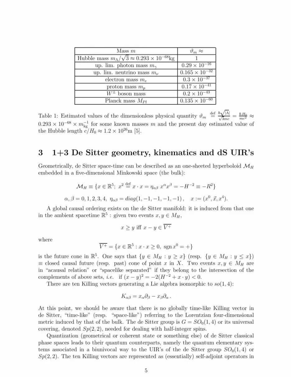
Mass m ϑm ≈Hubble mass mΛ/
√3 ≈ 0.293× 10−68kg 1
up. lim. photon mass mγ 0.29× 10⁻¹⁶
up. lim. neutrino mass mν 0.165× 10⁻³²
electron mass me 0.3× 10−37
proton mass mp 0.17× 10−41
W± boson mass 0.2× 10−43
Planck mass MP l 0.135× 10−60
Table 1: Estimated values of the dimensionless physical quantity ϑmdef=
~
√|Λ|√
3mc= ~H0
mc2≈
0.293 × 10−68 ×m−1kg for some known masses m and the present day estimated value of
the Hubble length c/H0 ≈ 1.2× 1026m [5].
3 1+3 De Sitter geometry, kinematics and dS UIR’s
Geometrically, de Sitter space-time can be described as an one-sheeted hyperboloid MH
embedded in a five-dimensional Minkowski space (the bulk):
MH ≡ {x ∈ R5; x2 def
= x · x = ηαβ xαxβ = −H−2 ≡ −R2}
α, β = 0, 1, 2, 3, 4, ηαβ = diag(1,−1,−1,−1,−1) , x := (x0, ~x, x4).
A global causal ordering exists on the de Sitter manifold: it is induced from that onein the ambient spacetime R5 : given two events x, y ∈MH ,
x ≥ y iff x− y ∈ V +
whereV + = {x ∈ R
5 : x · x ≥ 0, sgn x0 = +}is the future cone in R5. One says that {y ∈ MH : y ≥ x} (resp. {y ∈ MH : y ≤ x})≡ closed causal future (resp. past) cone of point x in X. Two events x, y ∈ MH arein “acausal relation” or “spacelike separated” if they belong to the intersection of thecomplements of above sets, i.e. if (x− y)2 = −2(H−2 + x · y) < 0.
There are ten Killing vectors generating a Lie algebra isomorphic to so(1, 4):
Kαβ = xα∂β − xβ∂α .
At this point, we should be aware that there is no globally time-like Killing vector inde Sitter, “time-like” (resp. “space-like”) referring to the Lorentzian four-dimensionalmetric induced by that of the bulk. The de Sitter group is G = SO0(1, 4) or its universalcovering, denoted Sp(2, 2), needed for dealing with half-integer spins.
Quantization (geometrical or coherent state or something else) of de Sitter classicalphase spaces leads to their quantum counterparts, namely the quantum elementary sys-tems associated in a biunivocal way to the UIR’s of the de Sitter group SO0(1, 4) orSp(2, 2). The ten Killing vectors are represented as (essentially) self-adjoint operators in
5

Hilbert space of (spinor-)tensor valued functions on MH , square integrable with respectto some invariant inner (Klein-Gordon type) product :
Kαβ → Lαβ = Mαβ + Sαβ ,
where Mαβ = −i(xα∂β − xβ∂α) (orbital part), and Sαβ (spinorial part) acts on indices offunctions in a certain permutational way. Note the usual commutation rules,
[Lαβ , Lγδ] = −i (ηαγLβδ − ηαδLβγ − ηβγLαδ + ηβδLαγ) . (9)
Two Casimir operators exist whose eigenvalues determine the UIR’s :
C2 = −1
2LαβLαβ , (10)
C4 = −WαW α, Wα = −1
8ǫαβγδηL
βγLδη , (11)
where (Wα) is the dS counterpart of the Pauli-Lubanski operator. These Wα’s transformlike vectors:
[Lαβ , Wγ] = i (ηβγWα − ηαγWβ) . (12)
In particular we haveWa = i [W0, La0, ] , a = 1, 2, 3, 4 . (13)
The Wα’s commute as:
[Wα, Wβ] = −iǫαβα1α2α3Wα1Lα2α3
= −i(LγδLγδ − 3
)Lαβ +
i
2
{Lγδ, {Lαγ , Lβδ}
}. (14)
The algebra defined by the Lαβ and the Wα generators (regarded as primitive generators)is a non-linear finite W -algebra [6]. This algebra respects the grading [Lαβ ] = 2, [Wα] = 3,[[, ]] = −1.
As it is the case with non-linear W -algebras, (9), (12) and (14) can be linearized (the“unfolded” version) at the price of introducing an infinite number of generators regarded asprimitive generators. E.g., the r.h.s. of Equation (14) can be written as −iǫαβγ1γ2γ3Z
γ1γ2γ3 ,where Zγ1γ2γ3 can be identified with W γ1Lγ2γ3 ([Zγ1γ2γ3 ] = 5). An infinite tower of extraprimitive generators have to be introduced to close the algebra linearly.
It is convenient to reexpress the Lαβ , Wα generators of the finite W -algebra in theirSO(4) decomposition, (a, b = 1, 2, 3, 4), given by Ta, Lab, Z, Wa, where
Tα = L0α , Z = W0 .
Due to the fact that the Wa’s arise from the commutator [Ta, Z], we can regard the finitenon-linear W -algebra with Ta, Lab, Z, Wa primitive generators as an unfolded version ofthe finite non-linear W -algebra with Ta, Lab, Z primitive generators.
The operator W0 is the difference of two commuting su(2)-Casimir. To get this, westart from the expression:
W0 = −(L12L34 + L23L14 + L31L24) = −J ·A .
6

The operators J = (L23, L31, L12)T and A = (L14, L24, L34)
T represent a basis for themaximal compact subalgebra k ∼= so(4):
[Ji, Jj ] = iJk , [Ji, Aj] = iAk , [Ai, Aj] = iJk ,
with (i, j, k) even permutation of (1, 2, 3). Introducing the two commuting sets of su(2)generators:
NL :=1
2(A + J), NR :=
1
2(A− J) ,
[N
LRi , N
LRj
]= ±iN
LR
k ,
we obtainW0 = −J ·A = −A · J = (NL)2 − (NR)2.
In consequence, as an operator on a direct sum of SU(2) UIR’s its spectrum is made ofthe numbers jl(jl+1)−jr(jr+1), jl, jr ∈ N/2. A complete classification [7] of the de SitterUIR’s is precisely based on the following property. Let Sp(2, 2) ∋ g 7→ ρ(g) ∈ Aut(H) aUIR of Sp(2, 2) acting in a Hilbert space H. Then the restriction to the maximal compact
subgroup Kdef= SU(2)× SU(2) is completely reducible:
H = ⊕(jl,jr)∈ΓρHjl,jr
, Hjl,jr∼= C
2jl+1 ×C2jr+1 ,
where Γρ ⊂ N/2 is the set of pairs (jl, jr) such that the UIR Djl ⊗Djr of K appears onceand only once in the the reduction of the restriction ρ |K . Let p = inf(jl,jr)∈Γρ
(jl + jr)and q0 = min(jl,jr)∈Γρ
jl+jr=p
(jr − jl), q1 = max(jl,jr)∈Γρ
jl+jr=p
(jr − jl). Then we have the following
exhaustive possibilities:
(i) q1 = p and q0 = −p, which correspond to elements of the principal and complemen-tary series, denoted by Υp,σ where σ ∈ (−2, +∞) (with restrictions according to thevalues of p in N/2);
(ii) q1 = p and 0 < q0 ≡ q ≤ p, which correspond to elements of the discrete series,denoted by Π+
p,q;
(iii) q0 = −p and 0 < −q1 ≡ q ≤ p, which correspond to elements of the discrete series,denoted by Π−
p,q;
(iv) q0 = q1 = 0 ≡ q , which correspond to elements lying at the bottom of the discreteseries, denoted by Πp,0.
Let us now give more details on these three different types of representations.
“Discrete series” Π±p,q
Parameter q has a spin meaning and the two Casimir are fixed as
C2 = (−p(p + 1)− (q + 1)(q − 2))I ,
C4 = (−p(p + 1)q(q − 1))I .
We have to distinguish between
7

(i) the scalar case Πp,0, p = 1, 2, · · · , which are not square integrable,
(ii) the spinorial case Π±p,q, q > 0, p = 1
2, 1, 3
2, 2, · · · , q = p, p−1, · · · , 1 or 1
2. For q = 1/2
the representations Π±p, 1
2
are not square-integrable.
“Principal series” Us,ν
Υp=s,σ=ν2+ 14≡ Us,ν , q =
1
2± iν , σ = q(1− q) .
p = s has a spin meaning and the two Casimir are fixed as
C2 = (σ + 2− s(s + 1))I = (9/4 + ν2 − s(s + 1))I ,
C4 = σ s(s + 1)I = (1/4 + ν2) s(s + 1)I .
We have to distinguish between
(i) ν ∈ R (i.e., σ ≥ 1/4), s = 1, 2, · · · , for the integer spin principal series,
(ii) ν 6= 0 (i.e., σ > 1/4), s = 12, 3
2, 5
2· · · , for the half-integer spin principal series.
In both cases, Us,ν and Us,−ν are equivalent. In the case ν = 0, i.e. q = 12, s = 1
2, 3
2, 5
2· · · ,
the representations are direct sums of two UIR’s in the discrete series:
Us,0 = Π+s, 1
2
⊕Π−
s, 12
.
“Complementary series” Vs,ν
Υp=s,σ= 14−ν2 ≡ Vs,ν, q =
1
2± ν ,
p = s has a spin meaning and the two Casimir are fixed as
C2 = (σ + 2− s(s + 1))I = (9/4− ν2 − s(s + 1))I ,
C4 = σ s(s + 1)I = (1/4− ν2) s(s + 1)I.
We have to distinguish between
(i) the scalar case V0,ν , ν ∈ R, 0 < |ν| < 32
(i.e., −2 < σ < 1/4),
(ii) the spinorial case Vs,ν , 0 < |ν| < 12
(i.e., 0 < σ < 1/4), s = 1, 2, 3, . . . .
In both cases, Vs,ν and Vs,−ν are equivalent.
4 Contraction limits or desitterian Physics from the
point of view of a Minkowskian observer
On a geometrical level, limH→0MH = M0, the Minkowski spacetime tangent to MH
at, say, the de Sitter origin point OH . Then, on an algebraic level, limH→0 Sp(2, 2) =P↑
+(1, 3) =M0 ⋊SL(2, C), the Poincare group. The ten de Sitter Killing vectors contractto their Poincare counterparts Kµν , Πµ, µ = 0, 1, 2, 3, after rescaling the four K4µ −→Πµ = HK4µ (“space-time contraction”). On a UIR level, the question is mathematicallymore delicate.
8

The massive case
For the massive case, the principal series representations only are involved (from whichthe name “de Sitter massive representations”). Introducing ν through σ = ν2 + 1/4 andthe Poincare mass m = νH , we have the following result [8, 10]:
Us,ν −→H→0,ν→∞ c>P>(m, s)⊕ c<P<(m, s),
where one of the “coefficients” among c<, c> can be fixed to 1 whilst the other one vanishes
and where P><(m, s) denotes the positive (resp. negative) energy Wigner UIR’s of the
Poincare group with mass m and spin s.
The massless case
Here we must distinguish between the scalar massless case, which involves the uniquecomplementary series UIR Υ0,0 to be contractively Poincare significant, and the helicity= s case where are involved all representations Π±
s,s, s > 0 lying at the lower limit of the
discrete series. The arrows → below designate unique extension. P><(0, s) denotes the
Poincare massless case with helicity s. Conformal invariance leads us to deal also withthe discrete series representations (and their lower limits) of the (universal covering ofthe) conformal group or its double covering SO0(2, 4) or its fourth covering SU(2, 2) [9].
These UIR’s are denoted by C><(E0, j1, j2), where (j1, j2) ∈ N/2×N/2 labels the UIR’s of
SU(2)× SU(2) and E0 stems for the positive (resp. negative) conformal energy.
• Scalar massless case :
C>(1, 0, 0) C>(1, 0, 0) ← P>(0, 0)
Υ0,0 → ⊕ H=0−→ ⊕ ⊕C<(−1, 0, 0) C<(−1, 0, 0) ← P<(0, 0),
• Spinorial massless case :
C>(s + 1, s, 0) C>(s + 1, s, 0) ← P>(0, s)
Π−s,s → ⊕ H=0−→ ⊕ ⊕
C<(−s− 1, s, 0) C<(−s− 1, s, 0) ← P<(0, s),
C>(s + 1, 0, s) C>(s + 1, 0, s) ← P>(0,−s)
Π+s,s → ⊕ H=0−→ ⊕ ⊕
C<(−s− 1, 0, s) C<(−s− 1, 0, s) ← P<(0,−s),
We can see from the above that there is energy ambiguity in de Sitter relativity,exemplified by the possible breaking of dS irreducibility into a direct sum of two PoincareUIR’s with positive and negative energy respectively. This phenomenon is linked to theexistence in the de Sitter group of the discrete symmetry that sends any point (x0,P) ∈MH into its mirror image (x0,−P) ∈ MH with respect to the x0-axis. Under such asymmetry the four generators L0a, a = 1, 2, 3, 4, (and particularly L04 which contractsto energy operator!) transform into their respective opposite −L0a, whereas the six Lab’sremain unchanged. All representations that are not listed in the above contraction limitshave either non-physical Poincare contraction limit or have no contraction limit at all.
9

In order to get a unifying description of the dS-Poincare contraction relations, thefollowing “mass” formula has been proposed by Garidi [11] in terms of the dS UIR pa-rameters p and q:
m2Gar = 〈C2〉dS − 〈C2p=q〉dS = [(p− q)(p + q − 1)]m2
H , mH = ~H/c2. (15)
The minimal value assumed by the eigenvalues of the first Casimir in the set of UIR inthe discrete series is precisely reached at p = q, which corresponds to the “conformal”massless case. The Garidi mass has the advantages to encompass all mass formulasintroduced within a de-sitterian context, often in a purely mimetic way in regard withtheir minkowskian counterparts.
Now, given a minkowskian mass m and a “universal” length R =√
3/Λ = c H−1,nothing prevents us to consider the dS UIR parameter ν (principal series), specific of a“physics” in constant-curvature space-time, as meromorphic functions of the dimensionlessphysical (in the minkowskian sense!) quantity ϑm, as was introduced in Equation (2) interms of various other quantities introduced in this context, Note that ϑm is also theratio of the Compton length of the minkowskian object of mass m considered at the limitwith the universal length R yielded by dS geometry. Thus, we may consider the followingLaurent expansions of the dS UIR parameter ν (principal series) in a certain neighborhoodof ϑm = 0:
ν = ν(ϑm) =1
ϑm
+ e0 + e1ϑm + · · · en(ϑm)n + · · · , (16)
with ϑm ∈ (0, ϑmax) (convergence interval). The coefficients en are pure numbers to bedetermined. We should be aware that nothing is changed in the contraction formulas fromthe point of view of a minkowskian observer, except that we allow to consider positive aswell as negative values of ν in a (positive) neighborhood of ϑm = 0: multiply (16) by ϑm
and go to the limit ϑm → 0. We recover asymptotically the relation
m = |ν|~H/c2 = |ν|~c
√|Λ|3
. (17)
As a matter of fact, the Garidi mass is a good example of such an expansion since it canbe rewritten as the following expansion in the parameter ϑm ∈ (0, 1/|s− 1/2|]:
ν =
√1
ϑ2m
− (s− 1/2)2 =1
ϑm
− (s− 1/2)2
(ϑm
2+ O(ϑ2
m)
), (18)
Note the particular symmetric place occupied by the spin 1/2 case with regard to thescalar case s = 0 and the boson case s = 1.
5 Fuzzy de Sitter space-time with Compton wave-
length
Examining the equation (11) that fixes the value of the quartic Casimir in terms of theoperators Wα it is tempting, if no natural, to introduce a non-commutative structure for
10

the dS spacetime by replacing the classical variables of the bulk xα with the suitablynormalized W α operators through the “fuzzy” variables xα
xα → xα = rW α, (19)
where r ([r] = l) has been introduced for dimensional reasons. In principle a different r hasto be introduced for any given irreducible representation characterized by p, q (thereforer ≡ rp,q).
The non-commutativity reads as follows
[xα, xβ ] = −irǫαβγ1γ2γ3 xγ1Lγ2γ3 (20)
and goes to zero in the limit r → 0.On the other hand, the dS inverse curvature R, arising from the classical constraint
− xαxα = R2, (21)
is replaced in the “fuzzy” case by the equation
− xαxα = −r2p(p + 1)q(q − 1), (22)
inducing the identification
R = r√−p(p + 1)q(q − 1). (23)
What is r? A natural interpretation consists in assuming it to be a Compton length lcmp
of the associated particle. The most immediate approach then consists in looking at theMinkowski limit fixing the Minkowskian observational mass mobs as the limit of the Garidimass. In this case we have to work with the principal series which allows taking the limitν →∞. We get that (15) can be rewritten as
mGar =~
cR
√(s− 1
2)2 + ν2. (24)
In agreement with (16), we assume for ν a dependence on R such as
ν(R) = c−1R + c0 +c1
R+
c2
R2+ . . . , (25)
and we can safely take the R→∞ limit in the r.h.s. and obtain
mobs =~
cc−1. (26)
We are now in the position to use as r in (23) the Compton length associated to theobservational mass mobs. Since we are working with the principal series, (23) can be inthis case expressed as
R0 =~
mobsc
√s(s + 1)(
1
4+ ν2) , (27)
11

where R0 = c/H0. The physical interpretation of the (observational) parameter ν is thefact that it connects the observational curvature of the dS spacetime with the observationalmass of the elementary system (for the given spin s > 0). We obtain
ν2 =
(R2
0m2obsc
2
~2− s(s + 1)
4
)1
s(s + 1). (28)
Since ν2 must be positive we end up with a constraint on the observational masses of themassive elementary systems with spin s > 0. The constraint is given by the relation
mobs ≥~
2c
√s(s + 1)
1
R0=
mH0
2
√s(s + 1). (29)
One can say that for all known massive particles this lowest bound is of the order of theobserved Hubble mass ≈ 1.6 10−42GeV. Combining the upper limit of Table 1 and thislowest limit, we obtain the allowed mass range for massive neutrinos:
≈ 1.2 10−42 GeV ≤ mn ≤≈ 9.7 10−11 GeV .
The lower bound (29) for the observational masses of spin s > 0 particles is basedon the present-day value for the Hubble constant and the associated curvature of theuniverse. It admits, however, a reversed lecture. Starting from the known observationalmasses of the particles with positive spin, it could allow putting an upper bound (whichcan have cosmological implications) on the curvature of the dS universe.
It is worth pointing out that the “de Sitter fuzzy Ansatz” implies a lower bound forthe observed masses of all massive particles of positive spin s. The lower bound does notdepend on the electric charge (positive, negative or vanishing) of the particles. It dependssmoothly on their spin s. For large spin s the lower bound grows linearly with s.
We refer to the construction of the fuzzy de Sitter spacetime discussed in this Sectionas “Scenario I”. In this scenario the Compton length has been defined in the limitingMinkowski spacetime. In the next Section we will discuss another scenario (referred to as“Scenario II”), such that the Compton length is defined in the de Sitter spacetime itself.
6 Fuzzy de Sitter and Garidi mass
Another interpretation of r consists in assuming it to be a Compton length lC of theassociated particle with its desitterian Garidi mass. The Compton length is in this casedefined in the de Sitter spacetime itsef. We refer to this scenario as “Scenario II”. Forthe irreducible representation characterized by p, q the Compton length is
lC =~
mGarc. (30)
Scenario II offers different possibilities of constraining the relevant p, q UIR’s whichsatisfy some given properties. We explicitly discuss two such cases. In the first case wehave
lC =~
cmH
√1
(p− q)(p + q − 1)= lP l
1
ϑP l
√1
(p− q)(p + q − 1)(31)
12

and
R
lP l
=1
ϑP l
√−p(p + 1)q(q − 1)
(p− q)(p + q − 1). (32)
For the principal series we can set
p = s,
q =1
2+ iν, (33)
where s is the spin and ν ∈ R. For this series we obtain that (32) reads as
R
lP l
=1
ϑP l
√√√√s(s + 1) + s(s+1)4ν2
1 + 4s2−4s+14ν2
≈ 1
ϑP l
√s(s + 1). (34)
The last equality holds in the limit ν →∞.On the other hand, it is possible to choose ν ∈ R such that the r.h.s. of (34) does not
depend on s. For s = 1 we get
√s(s+1)+ s(s+1)
4ν2
1+ 4s2−4s+14ν2
=√
2 no matter which is the value of ν. In
order to reproduce this value for any positive (half-)integer spin s, ν must be given by
ν =
√7s2 − 9s + 2
4s2 + 4s− 8. (35)
The above equation always admits real solutions (for s = 12, ν =
√328
, for s = 32, ν =
√1728
,
for s = 2, ν = 34, for s = 5
2, ν =
√10328
, . . . with, in the limit s→∞, ν →√
74).
In the massless case we have mGar = 0, which implies either p = q or p = 1 − q. Inboth cases
R = r√
p2(1− p2), (36)
which is positive only for p = 12
(we are dealing with the Π±12, 12
irrep). Therefore
R = r
√3
16. (37)
In order to obtain the “universal formula”
R
lP l
=1
ϑP l
√2 (38)
we have to fix r, the Compton length lC of the massless spin 12
system, to be given by
r ≡ lC =lP l
ϑP l
√32
3. (39)
13

Summarizing the results obtained so far, in the first case of Scenario II we can constrainthe p, q UIR’s such that the ratio R
lPlbetween the de Sitter curvature and the Planck
length becomes universal (i.e., the allowed p, q produce formula (38)).In a second case for Scenario II, the Compton length for the Hubble mass is associated
with the curvature R through
mH =~
cR. (40)
By assuming (40) we can reexpress the Garidi mass mGar in terms of p, q and the curvatureR (besides the constants c and ~). We obtain
mGar =~
cR
√(p− q)(p + q − 1). (41)
Since
R = r√−p(p + 1)q(q − 1), (42)
with r the Compton length associated to the Garidi mass (r = ~
mGarc), we end up with
the equality
R = R
√−p(p + 1)q(q − 1)
(p− q)(p + q − 1). (43)
In this case the constraint
−p(p + 1)q(q − 1)
(p− q)(p + q − 1)= 1 (44)
has to be satisfied, giving a restriction on the allowed (p, q) UIR’s.For the principal series (p = s, q = 1
2+ iν) the restriction corresponds to the equation
s(s + 1)(1
4+ ν2) = (s− 1
2)2 + ν2, (45)
which implies
ν2 =1
2
√3s2 − 5s + 1
s2 + s− 1. (46)
The above equation finds solutions for any positive spin s > 0.
7 Conclusions
In this work we described a natural fuzzyness of the de Sitter spacetime. In analogy towhat happens in the case of the fuzzy spheres, a non-commutative structure for dS canbe introduced by replacing the classical variables of the bulk with the dS analogs of thePauli-Lubanski operators, suitably normalized by a dimensional parameter which plays
14

the role of the Compton length and measures the granularity of the non-commutative dSspace-time. We adopt the point of view of the elementary system described by UIR’sof the de Sitter group (parametrized by the pair (p, q)) and determine the mathematicaland physical consequences of the “de Sitter fuzzy Ansatz”. Two different scenarios havebeen investigated according to the possibility that the Compton length of the elemen-tary system is described in the Minkowski limit of the de Sitter spacetime (Scenario I; inthis case the suitable UIR’s of the de Sitter spacetime belong to the principal series andthe UIR’s of the Poincare group are recovered in the limit ν → ∞) or in the de Sitterspacetime itself (Scenario II). The “fuzzy dS Ansatz” in Scenario I has some observationalimplications. The observed masses of all massive particles with spin s > 0 admits a lowerbound of the order of the Hubble mass. For large s the lower bound grows linearly withs. The lower bound is only function of the spin (not of the charge of the particles) andapplies in particular to the case of the massive neutrinos. In scenario II the Comptonlength is fixed in the de Sitter spacetime itself and grossly determines the number of finiteelements (“pixels” or “granularity”) of a de Sitter spacetime of a given curvature. InScenario II the allowed UIR’s (parametrized by p and q) are determined in accordancewith the properties that have to be required for the fuzzy dS spacetime. We discussed inparticular two cases. A first case such that the ratio R
lPlbetween the dS curvature and the
Planck length is universal. A second case such that the Compton length for the Hubblemass is given by the dS curvature.
Acknowledgments
This work was supported (F.T.) by Edital Universal CNPq, Proc. 472903/2008-0.J.P.G. is grateful to CBPF, where this work was completed, for hospitality.
References
[1] Newton T D and Wigner E P 1949 Localized States for Elementary Systems, Rev.Mod. Phys. 21 400
[2] Wigner E P 1939 On Unitary Representations of the Inhomogeneous Lorentz Group,Ann. Math. 40 149
[3] Kirillov A A (2004). Lectures on the Orbit Method. Providence, RI: American Math-ematical Society.
[4] Linder V P 2008 Resource Letter DEAU-1: Dark energy and the accelerat-ing universe, Am. J. Phys. 76 197; Caldwell R and Kamionkowski M 2009The Physics of Cosmic Acceleration, astro-ph.CO 0903.0866v1; see also the linkhttp://lambda.gsfc.nasa.gov/product/map/current/map
[5] Lahav O and Liddle A R 2006, review article for The Review of Particle Physics2006, in S. Eidelman et al. 2004 Physics Letters B592, 1 (see 2005 partial updatefor edition 2006, http://pdg.lbl.gov/)
15

[6] de Boer J and Tjin T 1993 Commun. Math. Phys. 158 485; ibidem 1994160 317
[7] Dixmier J 1961, Bull. Soc. Math. France, 89 9; Takahashi R 1963 Bull. Soc. Math.France, 91 289
[8] Mickelsson J and Niederle J 1972 Commun. Math. Phys., 27 167
[9] Barut A O and Bohm A 1970 J. Math. Phys., 11 2398
[10] Garidi T, Huguet E and Renaud J 2003 Phys. Rev. D, 67 124028, gr-qc/0304031
[11] Garidi T 2003 What is mass in desitterian Physics?, hep-th/0309104
[12] Gazeau J P and Lachieze-Rey M 2006 Proceedings of Sciences, POS (IC2006) 007
[13] Gazeau J P and Novello M 2008 The question of mass in (anti-) de Sitter spacetimesJ. Phys. A: Math. Theor. 41 304008
[14] Gazeau J P, Mourad J, and Queva J Fuzzy de Sitter space-times via coherent statesquantization Proceedings of the XXVIth Colloquium on Group Theorical Methodsin Physics, New York 2006 (to appear, 2009) quant-ph/0610222v1
16


