Embed Size (px)
Citation preview
A Network Coding Approach toEnergy Efficient Broadcasting:
from Theory to Practice
Christina Fragouli1
EPFLLausanne, Switzerland
Email: [email protected]
Jorg Widmer2
DoCoMo Euro-LabsMunich, Germany
Email: [email protected]
Jean-Yves Le BoudecEPFL
Lausanne, SwitzerlandEmail: [email protected]
Abstract— We show that network coding allows to realize en-ergy savings in a wireless ad-hoc network, when each node of thenetwork is a source that wants to transmit information to all othernodes. Energy efficiency directly affects battery life and thus is acritical design parameter for wireless networks. We propose animplementable method for performing network coding in sucha setting. We analyze theoretical cases in detail, and use theinsights gained to propose a practical, fully distributed methodfor realistic wireless ad-hoc scenarios. We address practical issuessuch as setting the forwarding factor, managing generations, andimpact of transmission range. We use theoretical analysis andpacket level simulation.
I. INTRODUCTION
Network coding is an area that has emerged in 2000 [1],[2], and has since then attracted an increasing interest, asit promises to have a significant impact in both the theoryand practice of networks. We can broadly define networkcoding as allowing intermediate nodes in a network to notonly forward but also process the incoming information flows.Combining independent information flows allows to bettertailor the information flow to the network environment andaccommodate the demands of specific traffic patterns.
The first paradigm that illustrated the usefulness of networkcoding established throughput benefits when multicasting overerror-free links. Today, we have realized that we can getbenefits not only in terms of throughput, but also in termsof complexity, scalability, and security. These benefits arepossible not only in the case of multicasting, but also forother network traffic configurations, such as multiple unicastcommunications. Moreover, they are not restricted to error-freecommunication networks, but can also be applied to sensornetworks, peer-to-peer systems, and optical networks.
In this paper we show that use of network coding allows torealize energy savings when broadcasting in wireless ad-hocnetworks. By broadcasting we refer to the problem where eachnode is a source that wants to transmit information to all othernodes. Such one-to-all communication is traditionally usedduring discovery phases, for example by routing protocols;
1This work was supported by FNS under award No. 200021-103836/1.2Part of this work was done while Jorg Widmer was with EPFL.
more recently, it has been described as a key mechanism forapplication layer communication in intermittently connectedad-hoc networks [3].
Energy efficiency directly affects battery life and thus is acritical design parameter for wireless ad-hoc networks. Opti-mizing broadcasting for energy efficiency has been extensivelystudied during the last decade. The problem of minimumenergy broadcasting is NP-complete [4] and a large numberof approximation algorithms exist. Usually, these are eitherbased on probabilistic algorithms (see for example [5], [6], [7])where packets are only forwarded with a certain probability,or some form of topology control (e.g., [8], [9], [10]) to formconnected dominating sets of forwarding nodes.
The new ingredient in this problem is that we can applyideas from the area of network coding. Use of networkcoding has been examined in the literature in conjunctionwith multicasting, when a single source transmits commoninformation to a subset of the nodes of the network. If we allowintermediate nodes to code, the problem of minimizing theenergy per bit when multicasting can be formulated as a linearprogram and thus accepts a polynomial-time solution [11]. Analternative formulation is presented in [12], where a distributedalgorithm to select the minimum-energy multicast tree isproposed. Broadcasting information from a single source toall nodes in the network is a special case of multicasting andthus the same results apply. The problem is also related to [13]and [14] in the special case of wireless ad-hoc networks. In[15] we quantified the energy savings that network coding hasthe potential to offer when broadcasting in ad-hoc wirelessnetworks. The analysis was over canonical configurations,and assuming perfect centralized protocols. We also presentedpreliminary simulation results over random networks.
In this paper we examine different aspects of the proposedsystem in detail, that are related to and motivated by prac-tical considerations. The emphasis of the paper is both inunderstanding the theoretically expected performance, and indeveloping algorithms using the insights gained. In particular,• We theoretically examine benefits in terms of energy effi-ciency that use of network coding can bring to this problemwithout idealized centralized scheduling, that is, when we
restrict our attention to distributed algorithms. Based on thisanalysis, we propose distributed algorithms that are tuned torandom networks.• We evaluate possible tradeoffs of parameters that arise in apractical systems such as the effect of the transmission range.• We also develop distributed algorithms that can be deployedin real networks; we address fundamental considerations suchas the choice of a forwarding factor, restricted complexity andmemory capabilities, and limited generation sizes.
We evaluate the performance of our algorithms both onsystematic networks (circular network and square grid, wherewe can find exact results) and on random, realistic networks(where we obtain simulation results).
The paper is organized as follows. Section II formallyintroduces the problem formulation and reviews previoustheoretical results. In Section III we present our proposeddistributed algorithms. Section IV discusses the effect ofchanging the transmission range. Section V develops algo-rithms for constrained complexity and memory requirements,and Section VI concludes the paper.
II. BACKGROUND MATERIAL
In this section we first formally introduce the problemformulation and notation. We then briefly review known resultsthat are related to our approach, and discuss how our workis placed in this framework. We also describe the simulationenvironment that we will use to evaluate our algorithms.
A. Problem Formulation
Consider a wireless ad hoc network with n nodes, whereeach node is a source that wants to transmit information toall other nodes. We are interested in the minimum amount ofenergy required to transmit one unit of information from asource to all receivers.
We assume that each node v can successfully broadcastone unit of information to all neighbors N(v) within a giventransmission range, through physical layer broadcast. We alsoassume that the transmission range is the same for all nodes.Thus, minimizing the energy is equivalent to minimizingthe number of transmissions required to convey a unit ofinformation from a source to all receivers.
More precisely, let Tnc denote the total number of transmis-sions required to broadcast one information unit to all nodeswhen we use network coding. Similarly, let Tw denote therequired number of transmissions when we do not use networkcoding. We are interested in calculating Tnc
Tw.
Note that the same problem formulation, minimizing thenumber of channel uses (transmissions) per information unit,can be equivalently viewed as maximizing the throughputwhen broadcasting. Thus our results can also be interpretedas bounding the throughput benefits that network coding canoffer, for our particular traffic and network environment.
Let x1, . . . xn denote the source symbols associated withthe n nodes. These symbols1 are over a finite field Fq. Each
1Equivalently, we can think of x1, . . . xn as packets of symbols, and applyto each packet the operations symbol-wise. In the following we will talk aboutsymbols and packets interchangeably.
linear combination y over Fq that a node transmits or receives,can be described as the product of a vector of coefficients anda vector of source symbols
y = ax = [a1 . . . an]
⎡⎢⎢⎣
x1
x2
. . .xn
⎤⎥⎥⎦ .
In the network coding literature, the n-dimensional vector ofcoefficients is referred to as a coding vector. Following theapproach in [16] we assume that packets (coded symbols) arealways sent together with the corresponding coding vectors.
In the following it will be convenient to think in terms ofvector spaces, and say that a node has received a vector spacespanned by m coding vectors, when the node has received them corresponding linear combinations of the source symbols.Each node v stores its source symbol and the informationvectors it receives, in a decoding matrix Gv , that containsthe tuples of the coding vectors and the received informationsymbols. The matrix of a source si that has not yet receivedinformation from any other node contains only a single row(ei, xi). A received packet is said to be innovative if its vectorincreases the rank of the matrix.
In the case of network coding, a node v will in generaltransmit a linear combination that lies in the vector spaceof its decoding matrix Gv . We can think of flooding orprobabilistic routing (i.e., without the use of network coding)as constraining the coding vectors to belong in the set of theorthonormal basis elements
e1 = [1 0 0 . . . 0], e2 = [0 1 0 . . . 0], . . . , en = [0 . . . 0 1].
Thus in this case Gv is a submatrix of the identity matrix.Once a node receives n linearly independent combinations,
or equivalently, a basis of the n-dimensional space, it is ableto decode and retrieve the information of the n sources. In thecase of network coding, decoding amounts to solving a systemof linear equations, with complexity bounded as O(n3). In thecase of probabilistic routing no decoding is required.
B. Previous Results
In [15] we evaluated the theoretical energy requirements forbroadcasting with and without network coding, over canonicalnetworks, and assuming perfect centralized scheduling. Moreprecisely, we characterized the optimal performance we mayhope to get over these canonical configurations with any trans-mission scheme, showed that it can be achieved using networkcoding, and also evaluated what fraction of this optimal valuewe can achieve using forwarding. For completeness we brieflyreview these results here.
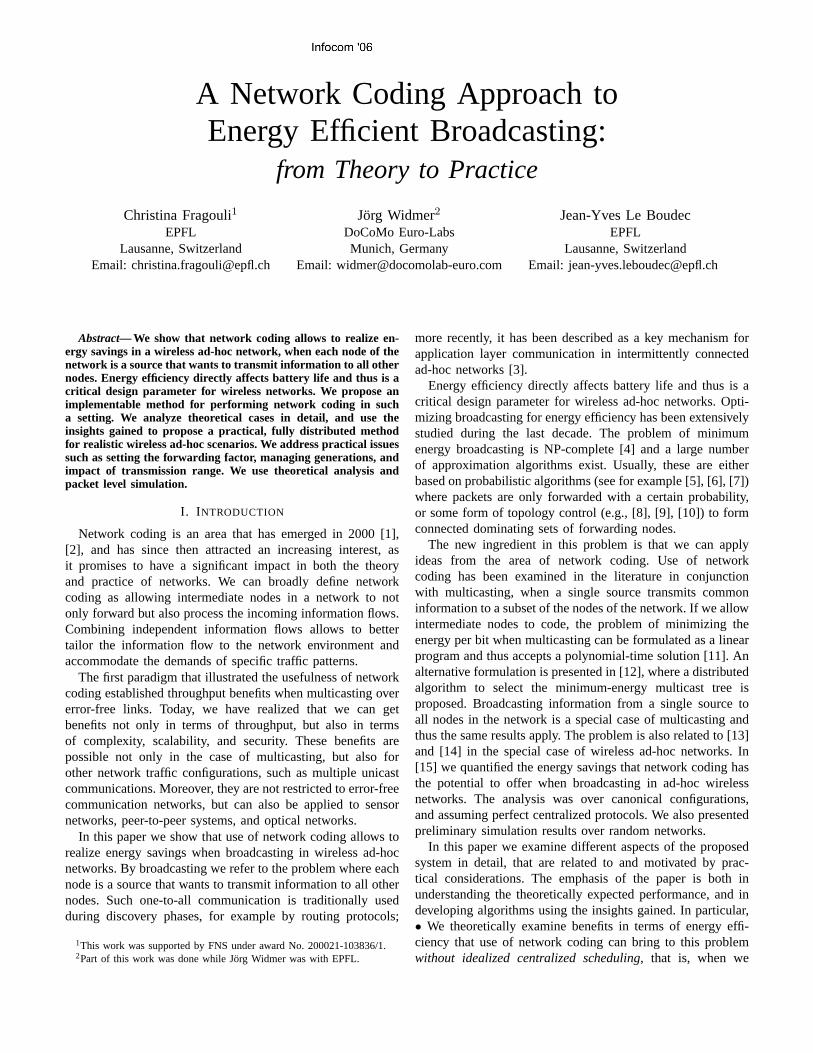
1. Circular Network: In the circular network n nodes areplaced at equal distances around a circle as depicted in Fig. 1.
Assume that each node can successfully broadcast informa-tion to its two nearest neighbors. For example, in Fig. 1, node 1can successfully broadcast information to nodes 2 and 8. In[15] it was shown that
1) without network coding Tw ≥ (n − 1) (1 + ε)2) with network coding Tnc ≥ n−1
2 (1 + ε),
2
12
3
45
6
7
8
Fig. 1. A circular configuration with 8 nodes.
where limn→∞ ε → 0. It was also shown that there existrouting and coding schemes that achieve the lower bound, andthus
Tnc
Tw=
12. (1)
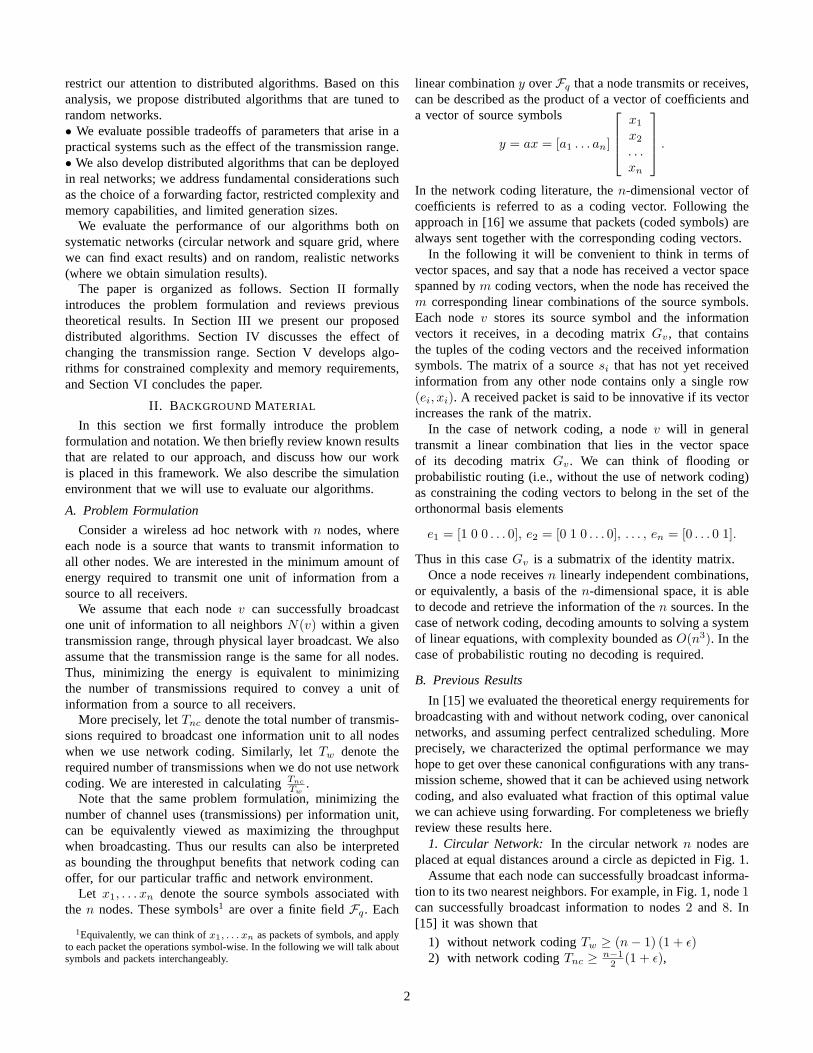
2. Square Grid Network: In this case we consider a wirelessad-hoc network with n = m2 nodes where the nodes areplaced on the vertices of a rectangular grid. To avoid edgeeffects, we will also assume that the area of the grid envelopesthe surface of a torus. In [15] it was shown that, if each
1
10 10
10
11 11
12 12
13
14 15 16
14 15 16 10
137
2
659
4
8 3
Fig. 2. A rectangular grid configuration. The node numbering expresses thefact that the grid envelopes a torus.
node can successfully broadcast information to its four nearestneighbors then
1) without network coding Tw ≥ n2
3 (1 + ε)2) with network coding Tnc ≥ n2
4 (1 + ε),where limn→∞ ε → 0 and that there exist schemes that achievethe lower bounds for Tw and Tnc. Thus
Tnc
Tw=
34. (2)
As is well known, random networks tend asymptotically (inthe number of nodes) to behave like square grid networks.We underline that the benefits calculated here refer to anidealized case, where perfect centralized scheduling of all nodetransmissions is possible. As we will see in the following sec-tions, in more realistic environments, network coding allowsto realize significantly larger gains when we constrain bothflooding and coding to operate in a distributed manner.
C. Description of the Simulator
Throughout this paper we will verify our theoretical analysisthrough simulation results over random topologies. Unlessexplicitly stated otherwise, the simulation environment willbe as described in the following.
Nodes have a nominal transmission range of ρ = 250m andare placed on a torus to avoid edge effects. Transmissions are
received by all the nodes within transmission range. We usea custom, time-based network simulator. A packet (symbol)transmission takes exactly one time unit. We assume that anode can either send or receive one packet at a time. TheMAC layer is an idealized version of IEEE 802.11 with perfectcollision avoidance. At each time unit, a schedule is createdby randomly picking a node and scheduling its transmissionif all of its neighbors are idle. This is repeated until no morenodes are eligible to transmit.
To allow an efficient implementation of network coding,we use operations over the finite field F28 , so that eachsymbol of the finite field can be stored in a byte. Additionand multiplication operations over this finite field can beimplemented using xor and two lookup tables of size 255bytes [17]. The encoding vectors are transported in the packetheader as suggested in [16]. We use randomized networkcoding, i.e., combine the received vectors uniformly at randomto create the vector to transmit.
As performance metrics we mainly use Packet DeliveryRatio (PDR) and decoding delay. The PDR is defined as thenumber of packets that can be decoded at the destination.For probabilistic routing, this is equal to the number ofreceived innovative packets, whereas with network coding, notall innovative packets can necessarily be decoded. Similarly,delay is counted as the average time between the transmissionof a packet by the original source and successful decodingat a node, where averaging is across receiver nodes. Forsome simulations we also investigate total network energyconsumption, which is measured as the sum of transmit power× transmission time over the duration of the simulation.
III. DISTRIBUTED ALGORITHMS
In this section we develop distributed algorithms that arewell suited for random topologies. To this goal, we firstprove that there exists a simple distributed algorithm that usesnetwork coding and allows to achieve the optimal performanceover the square grid network. We then tune this algorithmto perform well in a random topology, and verify throughsimulation that we obtain the expected benefits.
As discussed in Section II, in [15] we proved that thereexists a network coding scheme that achieves Tnc = n2
4 (1+ε),i.e., the minimum possible number of transmissions. However,the associated scheduling algorithm tends to be involved,andthus might be challenging to implement in a practical system.
In the following we describe a much simpler schedulingthat still allows us to achieve the optimal benefits in termsof energy efficiency. The algorithm operates in iterations asfollows.Algorithm 1:• Iteration 1: Each node broadcasts the information symbolit produces to its four closest neighbors.• Iteration k: Each node transmits a linear combination ofthe source symbols that belongs in the span of the codingvectors that the node has received in previous iterations.
3
A. Theoretical Analysis
Let mk denote the number of linear independent combina-tions that node i has received at the end of iteration k, and letV i
k be the vector space spanned by the corresponding codingvectors. That is, mk = |V i
k |. Moreover, if A is a set of nodes,denote by V A
k the union of the vector spaces that the nodesin A span, i.e., V A
k = {⋃j V jk , j ∈ A}.
To show that Algorithm 1 allows to achieve the optimalperformance when broadcasting, we need to show that thereexists a coding scheme (linear combinations that nodes cantransmit) such that each broadcast transmission brings innov-ative information to four receivers. This implies that Algorithm1 operates in k = 1 . . . �n
4 � iterations as follows. At iterationk, each node i
1) Transmits a vector from the vector space spanned by thecoding vectors the node received at iterations 1 . . . k−1.
2) Receives four vectors, from his four closest neighbors,and increases the size of its vector space by four.
Before the iterations begin, each node has its own sourcesymbol, and thus m0 = 1. Thus equivalently, it is sufficientto show that for each node i at the end of iteration k
mk = mk−1 + 4 = 4k + 1. (3)
To prove that there exists a coding scheme such that Eq. (3)holds, it is sufficient to prove that the following theorem holds.
Theorem 1: There exists a coding scheme to be used withAlgorithm 1 on the square grid such that at iteration k,
|V Ak | ≥ min{mk + |A| − 1, n} (4)
for any set A of nodes, where mk = 4k + 1, m0 = 1.Eq. (4) for A = {i} gives that |V i
k | ≥ mk = 4k +1. But nodei at iteration k has received only 4k broadcast transmissions,i.e., |V i
k | ≤ mk = 4k + 1. Thus the theorem directly impliesthat |V i
k | = mk = 4k + 1. For the proof of this theorem, wewill use two results, that we describe in Lemmas 1 and 2.
Lemma 1: Any set A of nodes in the grid,with 4+ |A| ≤ n,has at least four distinct neighbors.
Proof: The proof uses the fact that the vertex min-cutbetween any two nodes in a square grid is four. Let B be theset of nodes in the grid that are not in A. From assumption Bcontains at least four nodes. If all the nodes in B are neighborsof nodes in A we are done. Assume that there exist a node bin B that is not a neighbor of any node in A. Let a be anynode in A. Connect a and b through four vertex disjoint paths.On each such path there exists a distinct neighbor of A.
The second result we will need, was originally used in theframework of network coding in [18]. Here we write this resultin a form that is convenient for the proof of our theorem.
Lemma 2: Consider a family of n × n matricesA1, A2, . . ., Am that are parameterized by coefficientsp1, p2, . . ., pl. Assume that, for each matrix Ai, thereexist values p1, p2, . . ., pl over a field Fqi
such that thedeterminant of Ai over Fqi
is non zero, i.e., det(Ai) �= 0.Then, there exists a finite field Fq, and there exist values in Fq
for p1, p2, . . ., pl such that det(A1) �= 0, . . . , det(Am) �= 0.
For example, if
A1 =[
p2 p(1 − p)p(1 − p) p2
], and A2 =
[1 p1 1
],
then for p = 1, det(A1) �= 0 over F2, for p = 0, det(A2) �= 0over F2, and for p = 2, both det(A1) �= 0 and det(A2) �= 0over F3.Proof of Theorem 1We will prove this theorem using induction.• For k = 0, m0 = 1, since every node has one source symbol.• For k = 1, m1 = 5. Indeed, at the end of the first iterationeach node has received the information symbols from its fournearest neighbors. Selecting any A nodes, we will have theinformation from the A nodes themselves, and moreover fromall their closest neighbors, which, from Lemma 1, will amountto a union vector space of size at least m1 + |A|−1 = |A|+4.• Assume that the condition holds for k = l−1. It is sufficientto show that it holds for k = l.
Consider a set A. We want to show that |V Ak | ≥ mk−1 +
4 + |A| − 1 = mk + |A| − 1. From induction we know that|V A
k−1| ≥ mk−1 + |A| − 1. If |V Ak−1| ≥ mk−1 + 4 + |A| − 1
we are done. The only interesting cases are when |V Ak−1| =
mk−1 + i + |A| − 1, i = 0 . . . 3. We will prove here the casewhere |V A
k−1| = mk−1 + |A|− 1. For the other three cases thearguments are very similar.
Let B be the set that includes A and all the nearestneighbors of A. From Lemma 1 we know that B contains atleast four nodes that do not belong in A, say {b1, b2, b3, b4}.We want to show that when the nodes in {b1, b2, b3, b4}transmit during iteration k, they increase the rank of the set Aby four. (And in fact, of every other set they are neighbors.)But this holds by the following argument. From assumption,
|V {A,j}k−1 | ≥ mk−1 + |A|, for j ∈ {b1, b2, b3, b4}
|V {A,j,l}k−1 | ≥ mk−1 + |A| + 1, for j, l ∈ {b1, b2, b3, b4}
|V {A,j,l,z}k−1 | ≥ mk−1 + |A| + 2, for j, l, z ∈ {b1, b2, b3, b4}
|V {A,b1,b2,b3,b4}k−1 | ≥ mk−1 + |A| + 3.
Thus, nodes b1, b2, b3 and b4 have vectors v1 v2, v3 andv4 respectively such that vj /∈ V A
k−1, j = 1 . . . 4, andthe vector space spanned by them has dimension four, i.e.,| < v1, v2, v3, v4 > | = 4. Then, from Lemma 2, there existlinear combinations that nodes bi can transmit at iterationk such that the vector space of A (and in fact any set Aneighboring them) increases in size by four.
To conclude, we have proved that there exists a codingscheme such that the simple distributed scheduling of Al-gorithm 1 achieves the optimal theoretically performance. Inpractice we will use randomized coding over a large enoughfield [19], to approximate this optimal performance.
B. Application to Random Networks
In this section we extend Algorithm 1 to work over randomtopologies, where the number of neighbors N(v) of a node v isnot constant. Moreover, the network is not perfectly symmetricand we cannot assume perfect synchronization among nodes.
4

0
0.2
0.4
0.6
0.8
1
1005025136
Req
uire
d F
orw
ardi
ng F
acto
r (d
)
Avg. Number of Neighbors
Probabilistic RoutingNetwork Coding
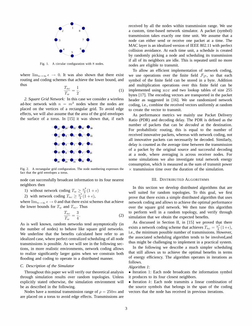
Fig. 3. Forwarding factor required to achieve a 99% PDR for different nodedensities (in a network of 2000m × 2000m)
To account for these factors, the authors in [15] proposeda network coding protocol in analogy to probabilistic routingalgorithms that forwards packets with a certain probability,according to a forwarding factor d > 0 [6], [7]. The forward-ing factor should intuitively be inversely proportional to thedensity of a node’s neighborhood. In [15] the forwarding factorreflected the average node density of the network. Figure 3shows which forwarding factor is required to achieve a 90%PDR with probabilistic routing and with network coding. Weobserve that the overhead of probabilistic routing is higher bya factor of 2-3, except for the case where the node densityis so low that a number of nodes have only one or very fewneighbors. In this case, network coding as well as probabilisticrouting need to use d = 1.
In this paper we extend this work by proposing to use adynamic forwarding factor, that is different for each node ofthe network, and adapts to possible changes of the networktopology. The algorithm can be described as follows.Algorithm 2:• Associate with each node v a “forwarding factor” dv .• Node v transmits its source symbol max{1, �dv} times, andan additional time with probability p = dv − max{1, �dv} ifp > 0.• When a node receives an innovative symbol, it broadcasts alinear combination over the span of the received coding vectors�dv times, and an additional time with probability p = dv −�dv if p > 0.
The optimum value of dv depends on the number of disjointpaths from the information sources to all other nodes and canonly be calculated with perfect knowledge of the networktopology. Since we are interested in simple algorithms, weassume that a node can acquire knowledge about the directneighborhood as well as the two-hop neighborhood, whilefurther information is too costly to gather. We will thereforeinvestigate the performance of two heuristics to adjust dv .
Let N(v) be the set of direct neighbors of node v and let kbe a forwarding factor to be used when a node only has onesingle neighbor. We scale dv as follows.• Algorithm 2A: Set v’s forwarding factor inversely propor-
tional to the number of 1-hop neighbors
dv =k
|N(v)| .
• Algorithm 2B: Set the forwarding factor inversely propor-tional to the minimum of the number of 1-hop neighbors ofv’s 1-hop neighbors
dv =k
minv′∈N(v) |N(v′)| .
We expect the second scheme to outperform the first.Intuitively, if a node v has multiple neighbors but one of theneighbors v′ has only node v as a neighbor, v needs to forwardall available information to v′, no matter how many neighborsv itself has.
The performance of Algorithm 2B depends on the valueof k. In essence, k is a cumulative forwarding factor sharedbetween all nodes within a given radio range. It corresponds tothe number of packets that are transmitted within this coveragearea as a response to the reception of an innovative packet,independent of the node density.
To determine k, we need to compute the probability that atransmitted packet is innovative. In [5], the authors analyze theprobability that the broadcast of a given message is innovativefor at least one neighbor when this message has already beenoverheard a certain number of times, for the case of flooding.This probability quickly drops to 0 for more than ca. 6 − 8overheard broadcasts of the same message. Therefore, k shouldbe set such that the number of broadcasts in an area is closeto this value and independent of the network density.
A similar analysis is possible for network coding. As arough approximation, let us assume that a node v and allbut one of its neighbors have all g information vectors, andone neighbor v′ has no information. We are interested in theprobability that after overhearing kg transmissions, a packetfrom v will be innovative for v′. In other words, v′ must havereceived fewer than g innovative packets from the other nodesand is not yet able to decode.2
We compute this probability as follows. Let D0 be a diskof radius 1 (we can take all transmission ranges equal to 1since the probability we are interested in is independent of thedistance unit chosen). Let j = kg, and D1, ...,Dj be j disks,also of radius 1, with centers in D0, drawn independently anduniformly in D0. Define Qg
j as the probability that a randompoint M in D0 is covered by fewer than g of the j disks. Ourupper bound is the probability Qg
kg. We show in appendix howto compute this in closed form. The results are illustrated inTable III-B. For fixed g and large k, we have the approximation
Qgkg ≈ 1.72029√
gke−0.321021gk. (5)
2In real scenarios, it is extremely unlikely that v′ overhears none of thepackets that its neighbors received previously to obtain their information.Furthermore, v′ may obtain the missing information through a neighbor thatis not within v’s transmission range. Also this case is not part of the analysis.Therefore, the analysis below is a worst case estimate that gives an upperbound on the probability of v′ not being able to decode after kg transmissions.
5
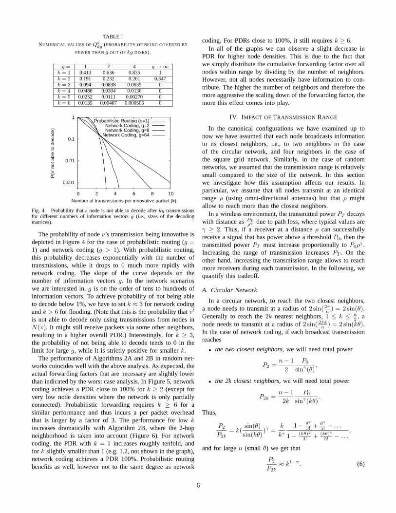
TABLE I
NUMERICAL VALUES OF Qgkg (PROBABILITY OF BEING COVERED BY
FEWER THAN g OUT OF kg DISKS).
g = 1 2 4 g → ∞k = 1 0.413 0.636 0.835 1k = 2 0.191 0.232 0.261 0.347k = 3 0.094 0.0838 0.0635 0k = 4 0.0480 0.0304 0.0136 0k = 5 0.0252 0.0111 0.00270 0k = 6 0.0135 0.00407 0.000505 0
0.001
0.01
0.1
1
0 2 4 6 8 10
P(v
’ not
abl
e to
dec
ode)
Number of transmissions per innovative packet (k)
Probabilistic Routing (g=1)Network Coding, g=2Network Coding, g=8
Network Coding, g=64
Fig. 4. Probability that a node is not able to decode after kg transmissionsfor different numbers of information vectors g (i.e., sizes of the decodingmatrices).
The probability of node v’s transmission being innovative isdepicted in Figure 4 for the case of probabilistic routing (g =1) and network coding (g > 1). With probabilistic routing,this probability decreases exponentially with the number oftransmissions, while it drops to 0 much more rapidly withnetwork coding. The slope of the curve depends on thenumber of information vectors g. In the network scenarioswe are interested in, g is on the order of tens to hundreds ofinformation vectors. To achieve probability of not being ableto decode below 1%, we have to set k ≈ 3 for network codingand k > 6 for flooding. (Note that this is the probability that v′
is not able to decode only using transmissions from nodes inN(v). It might still receive packets via some other neighbors,resulting in a higher overall PDR.) Interestingly, for k ≥ 3,the probability of not being able to decode tends to 0 in thelimit for large g, while it is strictly positive for smaller k.
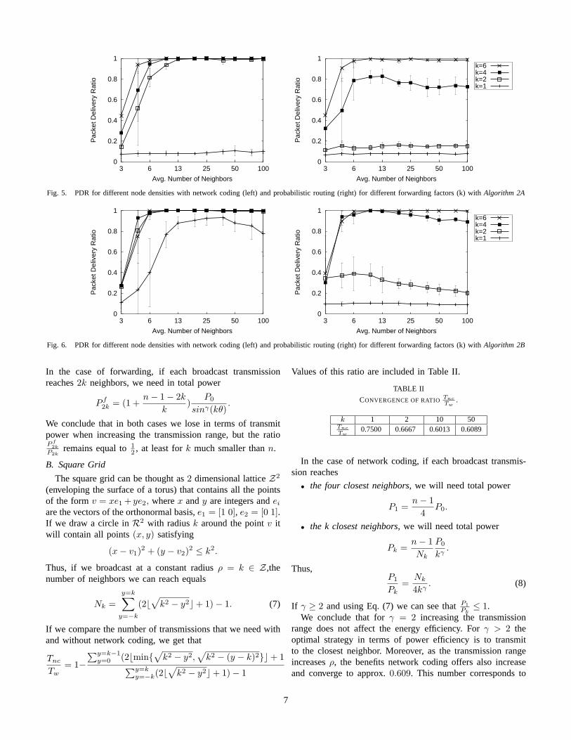
The performance of Algorithms 2A and 2B in random net-works coincides well with the above analysis. As expected, theactual forwarding factors that are necessary are slightly lowerthan indicated by the worst case analysis. In Figure 5, networkcoding achieves a PDR close to 100% for k ≥ 2 (except forvery low node densities where the network is only partiallyconnected). Probabilistic forwarding requires k ≥ 6 for asimilar performance and thus incurs a per packet overheadthat is larger by a factor of 3. The performance for low kincreases dramatically with Algorithm 2B, where the 2-hopneighborhood is taken into account (Figure 6). For networkcoding, the PDR with k = 1 increases roughly tenfold, andfor k slightly smaller than 1 (e.g. 1.2, not shown in the graph),network coding achieves a PDR 100%. Probabilistic routingbenefits as well, however not to the same degree as network
coding. For PDRs close to 100%, it still requires k ≥ 6.In all of the graphs we can observe a slight decrease in
PDR for higher node densities. This is due to the fact thatwe simply distribute the cumulative forwarding factor over allnodes within range by dividing by the number of neighbors.However, not all nodes necessarily have information to con-tribute. The higher the number of neighbors and therefore themore aggressive the scaling down of the forwarding factor, themore this effect comes into play.
IV. IMPACT OF TRANSMISSION RANGE
In the canonical configurations we have examined up tonow we have assumed that each node broadcasts informationto its closest neighbors, i.e., to two neighbors in the caseof the circular network, and four neighbors in the case ofthe square grid network. Similarly, in the case of randomnetworks, we assumed that the transmission range is relativelysmall compared to the size of the network. In this sectionwe investigate how this assumption affects our results. Inparticular, we assume that all nodes transmit at an identicalrange ρ (using omni-directional antennas) but that ρ mightallow to reach more than the closest neighbors.
In a wireless environment, the transmitted power PT decayswith distance as PT
ργ due to path loss, where typical values areγ ≥ 2. Thus, if a receiver at a distance ρ can successfullyreceive a signal that has power above a threshold P0, then thetransmitted power PT must increase proportionally to P0ρ
γ .Increasing the range of transmission increases PT . On theother hand, increasing the transmission range allows to reachmore receivers during each transmission. In the following, wequantify this tradeoff.
A. Circular Network
In a circular network, to reach the two closest neighbors,a node needs to transmit at a radius of 2 sin(2π
n ) = 2 sin(θ).Generally to reach the 2k nearest neighbors, 1 ≤ k ≤ n
2 , anode needs to transmit at a radius of 2 sin(2πk
n ) = 2 sin(kθ).In the case of network coding, if each broadcast transmissionreaches
• the two closest neighbors, we will need total power
P2 =n − 1
2P0
sinγ(θ),
• the 2k closest neighbors, we will need total power
P2k =n − 12k
P0
sinγ(kθ).
Thus,
P2
P2k= k(
sin(θ)sin(kθ)
)γ =k
kγ
1 − θ2
3! + θ4
5! − . . .
1 − (kθ)2
3! + (kθ)4
5! − . . .,
and for large n (small θ) we get that
P2
P2k≈ k1−γ . (6)
6
0
0.2
0.4
0.6
0.8
1
10050251363
Pac
ket D
eliv
ery
Rat
io
Avg. Number of Neighbors
0
0.2
0.4
0.6
0.8
1
10050251363
Pac
ket D
eliv
ery
Rat
io
Avg. Number of Neighbors
k=6k=4k=2k=1
Fig. 5. PDR for different node densities with network coding (left) and probabilistic routing (right) for different forwarding factors (k) with Algorithm 2A
0
0.2
0.4
0.6
0.8
1
10050251363
Pac
ket D
eliv
ery
Rat
io
Avg. Number of Neighbors
0
0.2
0.4
0.6
0.8
1
10050251363
Pac
ket D
eliv
ery
Rat
io
Avg. Number of Neighbors
k=6k=4k=2k=1
Fig. 6. PDR for different node densities with network coding (left) and probabilistic routing (right) for different forwarding factors (k) with Algorithm 2B
In the case of forwarding, if each broadcast transmissionreaches 2k neighbors, we need in total power
P f2k = (1 +
n − 1 − 2k
k)
P0
sinγ(kθ).
We conclude that in both cases we lose in terms of transmitpower when increasing the transmission range, but the ratioP f
2k
P2kremains equal to 1
2 , at least for k much smaller than n.
B. Square Grid
The square grid can be thought as 2 dimensional lattice Z2
(enveloping the surface of a torus) that contains all the pointsof the form v = xe1 + ye2, where x and y are integers and ei
are the vectors of the orthonormal basis, e1 = [1 0], e2 = [0 1].If we draw a circle in R2 with radius k around the point v itwill contain all points (x, y) satisfying
(x − v1)2 + (y − v2)2 ≤ k2.
Thus, if we broadcast at a constant radius ρ = k ∈ Z ,thenumber of neighbors we can reach equals
Nk =y=k∑
y=−k
(2�√
k2 − y2 + 1) − 1. (7)
If we compare the number of transmissions that we need withand without network coding, we get that
Tnc
Tw= 1−
∑y=k−1y=0 (2�min{
√k2 − y2,
√k2 − (y − k)2} + 1∑y=k
y=−k(2�√
k2 − y2 + 1) − 1
Values of this ratio are included in Table II.
TABLE II
CONVERGENCE OF RATIO TncTw
.
k 1 2 10 50TncTw
0.7500 0.6667 0.6013 0.6089
In the case of network coding, if each broadcast transmis-sion reaches
• the four closest neighbors, we will need total power
P1 =n − 1
4P0.
• the k closest neighbors, we will need total power
Pk =n − 1Nk
P0
kγ.
Thus,P1
Pk=
Nk
4kγ. (8)
If γ ≥ 2 and using Eq. (7) we can see that P1Pk
≤ 1.We conclude that for γ = 2 increasing the transmission
range does not affect the energy efficiency. For γ > 2 theoptimal strategy in terms of power efficiency is to transmitto the closest neighbor. Moreover, as the transmission rangeincreases ρ, the benefits network coding offers also increaseand converge to approx. 0.609. This number corresponds to
7
the area of the intersection of two circles with the same radiusand centers at distance equal to the radius.
C. Random Networks
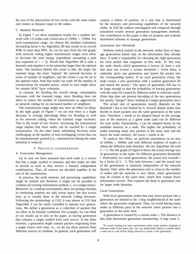
In Figure 7 we show simulation results for a random net-work with 144 nodes and a fixed area of 1500m × 1500m. Foreach transmission range, we choose the smallest cumulativeforwarding factor k for Algorithm 2B that results in an overallPDR of more than 99%. As can be seen from the left graph,with network coding higher transmission ranges even allowto decrease the total energy expenditure (assuming a pathloss exponent of γ = 2). Recall that Algorithm 2B is only aheuristic and requires k to be somewhat larger than the optimalvalue. The intuition behind this result is that, the larger thetransmit range, the more “regular” the network becomes interms of number of neighbors, and the closer k can be set tothe optimal value. Note that nodes can trade off the number oftransmissions for transmit power, which in turn might allowfor simpler MAC layer schedules.
In contrast, for flooding the overall energy consumptionincreases with the transmit range, since flooding does notallow to reduce the number of transmissions as aggressivelyas network coding for an increased number of neighbors.
The transmission range might also have an effect on delay.In the right graph of Figure 7 we see that there is a slightdecrease in average (decoding) delay for flooding as wellas for network coding, when the transmit range increases.This is the result of two factors: increasing the transmissionrange implies that more nodes can be reached by a singletransmission. On the other hand, scheduling becomes morechallenging, as the number of non-overlapping circles that canbe simultaneously packed (i.e., transmissions during the sametimeslot) is reduced.
V. PRACTICAL CONSIDERATIONS
A. Generation Management
Up to now we have assumed that each node is a sourcethat has a single symbol to transmit, and that nodes are ableto decode as soon as they receive n linearly independentcombinations. Thus, all sources are decoded together at theend of the transmission.
In practice, the node memory and processing capabilitiesmight be limited and therefore it might not be possible tocombine all existing information symbols xi in a single matrix.Moreover, in a random environment, there are perhaps benefitsin combining symbols not only across space, but also acrosstime, as is usually done in the network coding literature.Following the terminology in [16], it was shown in [15] thatAlgorithm 2 can be easily extended to operate over genera-tions. We define a generation as a collection of packets thatwe allow to be linearly combined. For example, we can thinkof our results up to now in the paper, as having generationthat contains a single symbol from each source. In the otherextreme, a generation might contain packets originating froma single source over time, i.e., we do not allow packets fromdifferent sources to combine. In general, each generation will
contain a subset of packets, of a size that is determinedby the memory and processing capabilities of the networknodes. In [20] the authors investigated and compared throughsimulation results several generation management methods.Our contribution in this paper is that we propose and evaluatedistributed schemes to manage generations.
Generation Size Threshold
Without central control in the network, nodes have to man-age generations based only on the information they alreadyhave. A node is responsible for choosing the right generationfor each packet that originates at this node. To this end,the node checks which generations it knows of, have a sizethat does not exceed a certain threshold t. From these, itrandomly picks one generation and inserts the packet intothe corresponding matrix. If no such generation exists, thenode creates a new generation with a random generation IDand inserts the packet.3 The space of generation IDs has tobe large enough so that the probability of having generationswith the same ID created by different nodes is relatively small.(Note that does not prevent decoding of the two generationsbut merely “merges” them, leading to a larger generation size.)
The actual size of generations merely depends on thethreshold t but is not limited by it. Several distant nodes maydecide to insert packets into the same generation at the sametime. Therefore, t needs to be adapted based on the averagesize of the matrices at a given node (and can be differentfor each node). Equivalently, t can be adapted based on theavailable memory at a node. The higher the probability ofnodes inserting many new packets at the same time and thelower the node memory, the lower t needs to be.
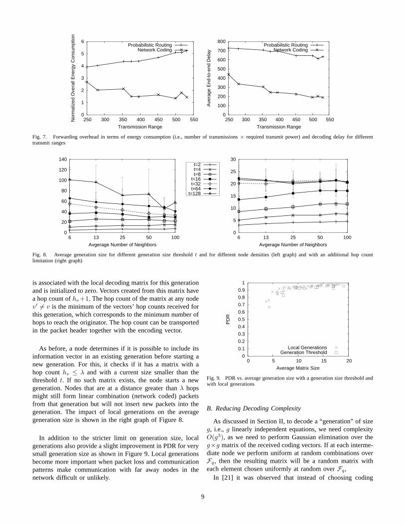
To analyze this effect, we perform simulations on an areaof 2000m × 2000m and with different numbers of nodes toobtain the different node densities. We use Algorithm 2B withk = 3. The left graph of Figure 8 shows the actual average sizeof generations at the nodes for different generation thresholdst. Particularly for small generations, the actual size exceeds tby a factor of 2 − 3. The ratio between t and the actual sizeof the generations is relatively independent of the networkdensity. Only when the generation size is close to the numberof nodes and the network is very dense, many generationsmay be created at the same time, which then contain fewerinformation vectors. This explains the drop in generation sizefor larger node densities.
Local Generations
With local generations, nodes that may insert packets into ageneration are limited to the λ-hop neighborhood of the nodewhere the generation originated. Thus, we avoid having manynodes in different parts of the network insert packets into ageneration at the same time.
A generation is created by a certain node v. The distance tothis node determines generation membership. A hop count hv
3To avoid creating too many generations when many packets originate atdifferent nodes at the same time, one can additionally impose a random delaya node has to wait before being allowed to create a new generation.
8
0
1
2
3
4
5
6
250 300 350 400 450 500 550Nor
mal
ized
Ove
rall
Ene
rgy
Con
sum
ptio
n
Transmission Range
Probabilistic RoutingNetwork Coding
0
100
200
300
400
500
600
700
800
250 300 350 400 450 500 550
Ave
rage
End
-to-
end
Del
ay
Transmission Range
Probabilistic RoutingNetwork Coding
Fig. 7. Forwarding overhead in terms of energy consumption (i.e., number of transmissions × required transmit power) and decoding delay for differenttransmit ranges
0
20
40
60
80
100
120
140
1005025136
Avgerage Number of Neighbors
t=2t=4t=8
t=16t=32t=64
t=128
0
5
10
15
20
25
30
1005025136
Avgerage Number of Neighbors
Fig. 8. Average generation size for different generation size threshold t and for different node densities (left graph) and with an additional hop countlimitation (right graph)
is associated with the local decoding matrix for this generationand is initialized to zero. Vectors created from this matrix havea hop count of hv +1. The hop count of the matrix at any nodev′ �= v is the minimum of the vectors’ hop counts received forthis generation, which corresponds to the minimum number ofhops to reach the originator. The hop count can be transportedin the packet header together with the encoding vector.
As before, a node determines if it is possible to include itsinformation vector in an existing generation before starting anew generation. For this, it checks if it has a matrix with ahop count hv ≤ λ and with a current size smaller than thethreshold t. If no such matrix exists, the node starts a newgeneration. Nodes that are at a distance greater than λ hopsmight still form linear combination (network coded) packetsfrom that generation but will not insert new packets into thegeneration. The impact of local generations on the averagegeneration size is shown in the right graph of Figure 8.
In addition to the stricter limit on generation size, localgenerations also provide a slight improvement in PDR for verysmall generation size as shown in Figure 9. Local generationsbecome more important when packet loss and communicationpatterns make communication with far away nodes in thenetwork difficult or unlikely.
0
0.1
0.2
0.3
0.4
0.5
0.6
0.7
0.8
0.9
1
0 5 10 15 20
PD
R
Average Matrix Size
Local GenerationsGeneration Threshold
Fig. 9. PDR vs. average generation size with a generation size threshold andwith local generations
B. Reducing Decoding Complexity
As discussed in Section II, to decode a “generation” of sizeg, i.e., g linearly independent equations, we need complexityO(g3), as we need to perform Gaussian elimination over theg×g matrix of the received coding vectors. If at each interme-diate node we perform uniform at random combinations overFq, then the resulting matrix will be a random matrix witheach element chosen uniformly at random over Fq,
In [21] it was observed that instead of choosing coding
9
vectors uniformly over Fq, in many cases we get comparableperformance by performing sparse linear combinations, overa small field. This work was motivated by the observation[22] that a sparse random matrix of size g × g(1 + ε)with limg→∞ ε
g = 0, has with high probability full rank. Inparticular, this is true if we choose each element of the matrixindependently to be one with probability p = log(g)
g , andzero otherwise. Moreover, such a matrix requires O(g2log(g))operations to be decoded. If each node in the graph performs“sparse” linear combinations, we can express the resultingmatrix that a receiver needs to decode as a product of sparsematrices which we can solve sequentially. Here we examinethe effect of reducing the alphabet size and of forming “sparse”linear combinations through simulation results.
Reducing the Alphabet Size: From simulations with 100nodes, a generation size of 100, and on average 12 neighborsper node, we see that a relatively small alphabet size issufficient to achieve good network coding performance. Onlythe field of size two, which is much smaller than the averagenumber of neighbors, provides an insufficient number oflinearly independent combinations per neighborhood. Alreadyan alphabet size of 22 comes close to the performance of analphabet size of 28 which is what we used in all of the previoussimulations.
0
0.2
0.4
0.6
0.8
1
3 2 1.5 1.25 1
PD
R
Cumulative Forwarding Factor (k)
F(2^1)F(2^2)F(2^4)F(2^8)
Fig. 10. Impact of reducing the alphabet size on PDR
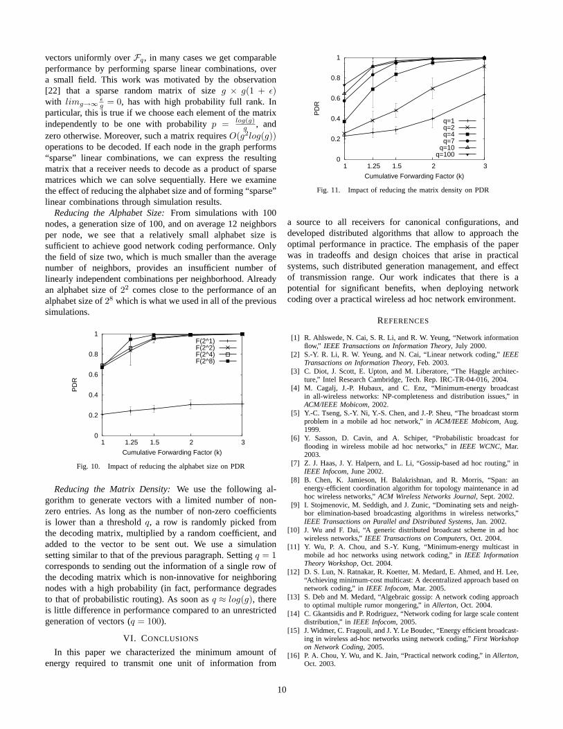
Reducing the Matrix Density: We use the following al-gorithm to generate vectors with a limited number of non-zero entries. As long as the number of non-zero coefficientsis lower than a threshold q, a row is randomly picked fromthe decoding matrix, multiplied by a random coefficient, andadded to the vector to be sent out. We use a simulationsetting similar to that of the previous paragraph. Setting q = 1corresponds to sending out the information of a single row ofthe decoding matrix which is non-innovative for neighboringnodes with a high probability (in fact, performance degradesto that of probabilistic routing). As soon as q ≈ log(g), thereis little difference in performance compared to an unrestrictedgeneration of vectors (q = 100).
VI. CONCLUSIONS
In this paper we characterized the minimum amount ofenergy required to transmit one unit of information from
0
0.2
0.4
0.6
0.8
1
3 2 1.5 1.25 1
PD
R
Cumulative Forwarding Factor (k)
q=1q=2q=4q=7
q=10q=100
Fig. 11. Impact of reducing the matrix density on PDR
a source to all receivers for canonical configurations, anddeveloped distributed algorithms that allow to approach theoptimal performance in practice. The emphasis of the paperwas in tradeoffs and design choices that arise in practicalsystems, such distributed generation management, and effectof transmission range. Our work indicates that there is apotential for significant benefits, when deploying networkcoding over a practical wireless ad hoc network environment.
REFERENCES
[1] R. Ahlswede, N. Cai, S. R. Li, and R. W. Yeung, “Network informationflow,” IEEE Transactions on Information Theory, July 2000.
[2] S.-Y. R. Li, R. W. Yeung, and N. Cai, “Linear network coding,” IEEETransactions on Information Theory, Feb. 2003.
[3] C. Diot, J. Scott, E. Upton, and M. Liberatore, “The Haggle architec-ture,” Intel Research Cambridge, Tech. Rep. IRC-TR-04-016, 2004.
[4] M. Cagalj, J.-P. Hubaux, and C. Enz, “Minimum-energy broadcastin all-wireless networks: NP-completeness and distribution issues,” inACM/IEEE Mobicom, 2002.
[5] Y.-C. Tseng, S.-Y. Ni, Y.-S. Chen, and J.-P. Sheu, “The broadcast stormproblem in a mobile ad hoc network,” in ACM/IEEE Mobicom, Aug.1999.
[6] Y. Sasson, D. Cavin, and A. Schiper, “Probabilistic broadcast forflooding in wireless mobile ad hoc networks,” in IEEE WCNC, Mar.2003.
[7] Z. J. Haas, J. Y. Halpern, and L. Li, “Gossip-based ad hoc routing,” inIEEE Infocom, June 2002.
[8] B. Chen, K. Jamieson, H. Balakrishnan, and R. Morris, “Span: anenergy-efficient coordination algorithm for topology maintenance in adhoc wireless networks,” ACM Wireless Networks Journal, Sept. 2002.
[9] I. Stojmenovic, M. Seddigh, and J. Zunic, “Dominating sets and neigh-bor elimination-based broadcasting algorithms in wireless networks,”IEEE Transactions on Parallel and Distributed Systems, Jan. 2002.
[10] J. Wu and F. Dai, “A generic distributed broadcast scheme in ad hocwireless networks,” IEEE Transactions on Computers, Oct. 2004.
[11] Y. Wu, P. A. Chou, and S.-Y. Kung, “Minimum-energy multicast inmobile ad hoc networks using network coding,” in IEEE InformationTheory Workshop, Oct. 2004.
[12] D. S. Lun, N. Ratnakar, R. Koetter, M. Medard, E. Ahmed, and H. Lee,“Achieving minimum-cost multicast: A decentralized approach based onnetwork coding,” in IEEE Infocom, Mar. 2005.
[13] S. Deb and M. Medard, “Algebraic gossip: A network coding approachto optimal multiple rumor mongering,” in Allerton, Oct. 2004.
[14] C. Gkantsidis and P. Rodriguez, “Network coding for large scale contentdistribution,” in IEEE Infocom, 2005.
[15] J. Widmer, C. Fragouli, and J. Y. Le Boudec, “Energy efficient broadcast-ing in wireless ad-hoc networks using network coding,” First Workshopon Network Coding, 2005.
[16] P. A. Chou, Y. Wu, and K. Jain, “Practical network coding,” in Allerton,Oct. 2003.
10
[17] C. H. Lim and P. J. Lee, “More flexible exponentiation with precom-putation,” in Proc. Advances in Cryptology: 14th Annual InternationalCryptology Conference, Aug. 1994.
[18] R. Koetter and M. Medard, “Beyond routing: an algebraic approach tonetwork coding,” in IEEE Infocom, June 2002.
[19] T. Ho, R. Koetter, M. Medard, D. R. Karger, and M. Effros, “The benefitsof coding over routing in a randomized setting,” in ISIT, June 2003.
[20] J. Widmer and J.-Y. Le Boudec, “Network coding for efficient communi-cation in extreme networks,” in Workshop on delay tolerant networkingand related networks (WDTN-05), Philadelphia, PA, Aug. 2005.
[21] C. F. Payam Pakzad and A. Shokrollahi, “Coding schemes for linenetworks,” ISIT, 2005.
[22] R. K. J. Blomer and E. Welzl, “The rank of sparse random matricesover finite fields,” Random Structures Algorithms 10, 1997.
APPENDIX: COMPUTATION OF COVERAGE PROBABILITY
Let D0 be a diskof radius 1. Let j = kg, and D1, ...,Dj bej disks, also of radius 1, with centers in D0, drawn indepen-dently and uniformly in D0. Define Qg
j as the probability thata random point M in D0 is covered by less than g of the jdisks. We are interested in Qg
kg . We have:
Qgj =
g−1∑i=0
qij (9)
with qij equal to the probability that a random point in D0 is
covered by exactly i of the j disks. Further:
qij =
∫D0
P (m is covered by exactly i of the j disks)dm
π(10)
By independence of D1,..., Dj :
qij =
∫D0
(ji
)(1 − P(m /∈ D1))
i (P(m /∈ D1))j−i dm
π(11)
We now compute P(m /∈ D1). By circular symmetry, itdepends only on the distance ρ = ‖m‖ from 0 to m. Let p1(ρ)be the value of P(m /∈ D1) when ‖m‖ = ρ. To compute p1(ρ)we first compute p(ρ, r), defined as the probability that m /∈D1 given that the distance from the center of D1 to the originis r. This is obtained by considering a random experimentwhere we select the center ω1 of D1 uniformly on the circlecentered at 0 with radius r. Let θ be the principal measure ofthe angle from �Oω1 to �Om. Let θmax be the maximum valueof θ such that m ∈ D1. We have{
if r + ρ > 1 then θmax = arccos r2+ρ2−12rρ
else θmax = π(12)
andp(ρ, r) = 1 − 2θmax
2π= 1 − θmax
π(13)
Thus (taking into account that r is a polar coordinate):
p1(ρ) = 2∫ 1
0p(ρ, r)rdr
= 2∫ 1
1−ρr(1 − 1
π arccos r2+ρ2−12rρ
)dr
= ρ√
4−ρ2+4 arcsin ρ2
2π
(14)
and
qij = 2
(ji
)∫ 1
0
(1 − p1(ρ))i (p1(ρ))j−iρdρ (15)
The integral in Equation (15) can be computed in closed formfor every fixed value of i and j. Note that Q1
j = q0j is the
probability of no coverage by j disks, which was computedexactly for j = 1 and by simulation for larger j in [5]. Incontrast, we obtain exact closed forms for all values of i andj. For example the first values of Q1
j = q0j are:
q01 = 3
√3
4π
q02 = −5+3
√3π
6π2
q03 = −351
√3+152π+24
√3π2
96π3
q04 = 21343−7020
√3π+1520π2+160
√3π3
1440π4
q05 = 4004397
√3−1363380π−210600
√3π2+30400π3+2400
√3π4
51840π5
We can also compute limits for large g or large k. We haveQg
j = 2∫ 1
0B(kg, g, 1 − p1(ρ))ρdρ where B(j, g, p) is the
(binomial) probability that a random experiment with successproability p succeeds less than g times in j experiments.For large k or g, we can approximate B(kg, g, p) by anormal distribution, which gives (Q(x) is the probability thata standard normal random variable is larger than x)
Qgkg ≈ 2
∫ 1
0
(1 − Q
(√
g1 − k(1 − p1(ρ)√k(1 − p1(ρ))p1(ρ)
)ρdρ
≈ 2∫ 1
0
Q
(√gk
√1
p1(ρ)− 1
)ρdρ (16)
=2√2π
∫ 1
0
∫ ∞√
gk�
1p1(ρ)−1
e−s22 dsdρ (17)
By inversion of the order of integration, one obtains
Qgkg ≈ 2
∫ ∞√
gkγ
e−s22 (1 − φ(s)2)ds (18)
where φ(s) is implicitly defined by p1(φ(s)) = 1√1+s2/gk
and
γ =√
1p1(1)
− 1 ≈ 0.642042. This function increases from 0
(for s = s0 =√
gkγ) to 1 for s → ∞; we approximate itwith the piecewise linear function given by the derivative ats0 and the asymptote which corresponds to φ(s) close to 1.One obtains the approximation 1 − φ(s)2 ≈ (s − s0) α√
gkfor
s0 ≤ s ≤√
gkα + s0 with
α =
(√3 + 2π
3
)2√ 13
(−1 + 6π
3√
3+2π
)π
≈ 2.15607
and otherwise 1 − φ(s)2 ≈ 1. The resulting integral can becomputed and one finds
Qgkg ≈ 2α√
2πgke−
12 gkγ =
1.72029√gk
e−0.321021gk (19)
With a similar analysis, for large g, we have the followinglimits, when k is fixed:
• For k = 1: limg→∞ Qgg = 1
• For k = 2, limg→∞ Qg2g = 1 − ρ2
1 ≈ 0.347224 where ρ1
is the root in (0, 1) of the equation p1(ρ1) = 1/2.• For k ≥ 3: limg→∞ Qg
g = 0
11


