Embed Size (px)
Citation preview

this print for reference only—size & color not accurate 7.5" x 9" / Casebound / Malloyspine bulk = 1.5625" 840 page count 50# Thor
Inside you’ll learn:
• The fundamentals of creative computer programming—from procedural programming, to object-oriented programming, to pure Java™ programming
• How to virtually draw, paint, and sculpt using computer code and clearly explained mathematical concepts
• 2D and 3D programming techniques, motion design, and cool graphics effects
• How to code your own pixel-level imaging effects, such as image contrast, color saturation, custom gradients and more
• Advanced animation techniques, including realistic physics and artificial life simulation
If you’re interested in creating cutting-edge code-based art and animations, you’ve come to the right place! Processing (available at http://processing.org) is a revolutionary open source programming language and environment designed to bridge the gap between programming and art, allowing non-programmers to learn programming fundamentals as easily as possible, and empowering anyone to produce beautiful creations using math patterns. With the software freely available, Processing provides an accessible alternative to using Flash for creative coding and computational art—both on and off the Web.
This book is written especially for artists, designers, and other cre-ative professionals and students exploring code art, graphics pro-gramming, and computational aesthetics. The book provides a solid and comprehensive foundation in programming, including object-orient-ed principles, and introduces you to the easy-to-grasp Processing language,
so no previous coding experience is necessary. The book then goes through using Processing to code lines, curves, shapes, and
motion, continuing to the point where you’ll have mastered Processing and can really start to unleash your creativity with realistic physics, interactivity, and 3D! In the final chapter, you’ll even learn how to extend your Processing skills by working directly
with the powerful Java™ programming language—the language Processing itself is built with.
GREENBERG
PRO
CESSIN
GMac/PC compatible
www.friendsofed.com
ISBN-13: 978-1-59059-617-3ISBN-10: 1-59059-617-X
9 781590 596173
90000
SHELVING CATEGORY1. GRAPHICS PROGRAMMING
IRA GREENBERG
ProcessingCreative Coding and Computational Art
CREATE CODE ART, VISUALIZATIONS,
AND INTERACTIVE APPLICATIONS WITH THIS
POWERFUL YET SIMPLE COMPUTER LANGUAGE AND PROGRAMMING
ENVIRONMENT.
LEARN HOW TO CODE 2D AND 3D
ANIMATION, PIXEL-LEVEL IMAGING, MOTION
EFFECTS, AND PHYSICS SIMULATIONS.
TAKE A CREATIVE AND FUN APPROACH
TO LEARNING CREATIVE COMPUTER
PROGRAMMING.
Foreword by Keith Peters

ProcessingCreative Coding and
Computational Art
Ira Greenberg
617xFM.qxd 5/2/07 12:05 PM Page i

Processing: Creative Coding andComputational Art
Copyright © 2007 by Ira Greenberg
All rights reserved. No part of this work may be reproduced or transmitted in any form or by any means,electronic or mechanical, including photocopying, recording, or by any information storage or retrieval
system, without the prior written permission of the copyright owner and the publisher.
ISBN-13: 978-1-59059-617-3
ISBN-10: 1-59059-617-X
Printed and bound in the United States of America 9 8 7 6 5 4 3 2 1
Trademarked names may appear in this book. Rather than use a trademark symbol with every occurrenceof a trademarked name, we use the names only in an editorial fashion and to the benefit of the trademark
owner, with no intention of infringement of the trademark.
Distributed to the book trade worldwide by Springer-Verlag New York, Inc., 233 Spring Street, 6th Floor,New York, NY 10013. Phone 1-800-SPRINGER, fax 201-348-4505, e-mail [email protected], or
visit www.springeronline.com.
For information on translations, please contact Apress directly at 2855 Telegraph Avenue, Suite 600,Berkeley, CA 94705. Phone 510-549-5930, fax 510-549-5939, e-mail [email protected], or
visit www.apress.com.
The information in this book is distributed on an “as is” basis, without warranty. Although every precautionhas been taken in the preparation of this work, neither the author(s) nor Apress shall have any liability to
any person or entity with respect to any loss or damage caused or alleged to be caused directly orindirectly by the information contained in this work.
The source code for this book is freely available to readers at www.friendsofed.com in theDownloads section.
Credits
Lead EditorChris Mills
Technical EditorCharles E. Brown
Technical ReviewersCarole Katz, Mark Napier
Editorial BoardSteve Anglin, Ewan Buckingham, Gary Cornell,
Jason Gilmore, Jonathan Gennick, Jonathan Hassell, James Huddleston, Chris Mills, Matthew Moodie,
Jeff Pepper, Dominic Shakeshaft, Matt Wade
Project ManagerSofia Marchant
Copy Edit ManagerNicole Flores
Copy EditorDamon Larson
Assistant Production DirectorKari Brooks-Copony
Production EditorEllie Fountain
CompositorDina Quan
ArtistMilne Design Services, LLC
ProofreadersLinda Seifert and Nancy Sixsmith
IndexerJohn Collin
Interior and Cover DesignerKurt Krames
Manufacturing DirectorTom Debolski
617xFM.qxd 5/2/07 12:05 PM Page ii

To Robin, Ian, and Sophie.
617xFM.qxd 5/2/07 12:05 PM Page iii

CONTENTS AT A GLANCE
Foreword . . . . . . . . . . . . . . . . . . . . . . . . . . . . . . . . . . . . . . . . . . . . . . xvAbout the Author . . . . . . . . . . . . . . . . . . . . . . . . . . . . . . . . . . . . . . . xviiAbout the Tech Reviewers . . . . . . . . . . . . . . . . . . . . . . . . . . . . . . . . xviiiAcknowledgments . . . . . . . . . . . . . . . . . . . . . . . . . . . . . . . . . . . . . . . xixIntroduction . . . . . . . . . . . . . . . . . . . . . . . . . . . . . . . . . . . . . . . . . . . . xx
PART ONE: THEORY OF PROCESSING AND COMPUTATIONAL ART . . . . 1
Chapter 1: Code Art . . . . . . . . . . . . . . . . . . . . . . . . . . . . . . . . . . . . . . . 3Chapter 2: Creative Coding . . . . . . . . . . . . . . . . . . . . . . . . . . . . . . . . 27Chapter 3: Code Grammar 101. . . . . . . . . . . . . . . . . . . . . . . . . . . . . . 57Chapter 4: Computer Graphics, the Fun, Easy Way . . . . . . . . . . . . . . 107Chapter 5: The Processing Environment . . . . . . . . . . . . . . . . . . . . . . 143
617xFM.qxd 5/2/07 12:05 PM Page iv

PART TWO: PUTTING THEORY INTO PRACTICE . . . . . . . . . . . . . . . . . 171
Chapter 6: Lines . . . . . . . . . . . . . . . . . . . . . . . . . . . . . . . . . . . . . . . . 173Chapter 7: Curves. . . . . . . . . . . . . . . . . . . . . . . . . . . . . . . . . . . . . . . 241Chapter 8: Object-Oriented Programming . . . . . . . . . . . . . . . . . . . . 301Chapter 9: Shapes . . . . . . . . . . . . . . . . . . . . . . . . . . . . . . . . . . . . . . 339Chapter 10: Color and Imaging . . . . . . . . . . . . . . . . . . . . . . . . . . . . . 399Chapter 11: Motion . . . . . . . . . . . . . . . . . . . . . . . . . . . . . . . . . . . . . 481Chapter 12: Interactivity . . . . . . . . . . . . . . . . . . . . . . . . . . . . . . . . . . 563Chapter 13: 3D . . . . . . . . . . . . . . . . . . . . . . . . . . . . . . . . . . . . . . . . . 615
PART THREE: REFERENCE . . . . . . . . . . . . . . . . . . . . . . . . . . . . . . . . . 673
Appendix A: Processing Language API . . . . . . . . . . . . . . . . . . . . . . . 675Appendix B: Math Reference . . . . . . . . . . . . . . . . . . . . . . . . . . . . . . 747
Index . . . . . . . . . . . . . . . . . . . . . . . . . . . . . . . . . . . . . . . . . . . . . . . . 775
617xFM.qxd 5/2/07 12:05 PM Page v

CONTENTS
Foreword . . . . . . . . . . . . . . . . . . . . . . . . . . . . . . . . . . . . . . . . . . . . . . xvAbout the Author . . . . . . . . . . . . . . . . . . . . . . . . . . . . . . . . . . . . . . . xviiAbout the Tech Reviewers . . . . . . . . . . . . . . . . . . . . . . . . . . . . . . . . xviiiAcknowledgments . . . . . . . . . . . . . . . . . . . . . . . . . . . . . . . . . . . . . . . xixIntroduction . . . . . . . . . . . . . . . . . . . . . . . . . . . . . . . . . . . . . . . . . . . . xx
PART ONE: THEORY OF PROCESSING AND COMPUTATIONAL ART . . . . 1
Chapter 1: Code Art . . . . . . . . . . . . . . . . . . . . . . . . . . . . . . . . . . . . . . . 3Aesthetics + Computation . . . . . . . . . . . . . . . . . . . . . . . . . . . . . . . . . . . . . 5Computer art history . . . . . . . . . . . . . . . . . . . . . . . . . . . . . . . . . . . . . . . . 8Code artists. . . . . . . . . . . . . . . . . . . . . . . . . . . . . . . . . . . . . . . . . . . . . 14
Ben Laposky, 1914–2000 . . . . . . . . . . . . . . . . . . . . . . . . . . . . . . . . . . . 14John Whitney Sr., 1918–1995. . . . . . . . . . . . . . . . . . . . . . . . . . . . . . . . . 15Herbert W. Franke, b.1927 . . . . . . . . . . . . . . . . . . . . . . . . . . . . . . . . . . 15Lillian Schwartz, b. 1927 . . . . . . . . . . . . . . . . . . . . . . . . . . . . . . . . . . . 15Harold Cohen, b. 1928 . . . . . . . . . . . . . . . . . . . . . . . . . . . . . . . . . . . . 16Roman Verostko, b. 1929. . . . . . . . . . . . . . . . . . . . . . . . . . . . . . . . . . . 17George Legrady, b. 1950 . . . . . . . . . . . . . . . . . . . . . . . . . . . . . . . . . . . 18Mark Napier, b. 1961 . . . . . . . . . . . . . . . . . . . . . . . . . . . . . . . . . . . . . 18John F. Simon Jr., b. 1963 . . . . . . . . . . . . . . . . . . . . . . . . . . . . . . . . . . . 19John Maeda, b. 1966 . . . . . . . . . . . . . . . . . . . . . . . . . . . . . . . . . . . . . 19Mary Flanagan, b. 1969 . . . . . . . . . . . . . . . . . . . . . . . . . . . . . . . . . . . . 20Casey Reas, b. 1970 . . . . . . . . . . . . . . . . . . . . . . . . . . . . . . . . . . . . . . 21Jared Tarbell, b. 1973 . . . . . . . . . . . . . . . . . . . . . . . . . . . . . . . . . . . . . 21Ben Fry, b. 1975 . . . . . . . . . . . . . . . . . . . . . . . . . . . . . . . . . . . . . . . . 22And many more . . . . . . . . . . . . . . . . . . . . . . . . . . . . . . . . . . . . . . . . 23
Summary . . . . . . . . . . . . . . . . . . . . . . . . . . . . . . . . . . . . . . . . . . . . . . 24
617xFM.qxd 5/2/07 12:05 PM Page vi

Chapter 2: Creative Coding . . . . . . . . . . . . . . . . . . . . . . . . . . . . . . . . 27The origin of Processing . . . . . . . . . . . . . . . . . . . . . . . . . . . . . . . . . . . . . 30Programming language comparisons . . . . . . . . . . . . . . . . . . . . . . . . . . . . . . 31
Function-based (procedural) vs. object-oriented structure . . . . . . . . . . . . . . . . 32Java . . . . . . . . . . . . . . . . . . . . . . . . . . . . . . . . . . . . . . . . . . . . . . . 36
Procedural OOP (“poop”) approach . . . . . . . . . . . . . . . . . . . . . . . . . . . . . . . 39Algorithms aren’t as scary as they sound . . . . . . . . . . . . . . . . . . . . . . . . . . . . 40Happy coding mistakes . . . . . . . . . . . . . . . . . . . . . . . . . . . . . . . . . . . . . . 44Algorithmic tree . . . . . . . . . . . . . . . . . . . . . . . . . . . . . . . . . . . . . . . . . . 45Summary . . . . . . . . . . . . . . . . . . . . . . . . . . . . . . . . . . . . . . . . . . . . . . 54
Chapter 3: Code Grammar 101. . . . . . . . . . . . . . . . . . . . . . . . . . . . . . 57Structure and abstraction . . . . . . . . . . . . . . . . . . . . . . . . . . . . . . . . . . . . . 58Your first program . . . . . . . . . . . . . . . . . . . . . . . . . . . . . . . . . . . . . . . . . 59
Curly braces . . . . . . . . . . . . . . . . . . . . . . . . . . . . . . . . . . . . . . . . . . 61Dot syntax . . . . . . . . . . . . . . . . . . . . . . . . . . . . . . . . . . . . . . . . . . . 62Naming conventions . . . . . . . . . . . . . . . . . . . . . . . . . . . . . . . . . . . . . 63
Literals . . . . . . . . . . . . . . . . . . . . . . . . . . . . . . . . . . . . . . . . . . . . . . . 64Variables . . . . . . . . . . . . . . . . . . . . . . . . . . . . . . . . . . . . . . . . . . . . . . 65
Strict typing . . . . . . . . . . . . . . . . . . . . . . . . . . . . . . . . . . . . . . . . . . 66Operators. . . . . . . . . . . . . . . . . . . . . . . . . . . . . . . . . . . . . . . . . . . . . . 72
Relational operators . . . . . . . . . . . . . . . . . . . . . . . . . . . . . . . . . . . . . 73Conditional operators. . . . . . . . . . . . . . . . . . . . . . . . . . . . . . . . . . . . . 74Assignment operators. . . . . . . . . . . . . . . . . . . . . . . . . . . . . . . . . . . . . 75
Conditionals . . . . . . . . . . . . . . . . . . . . . . . . . . . . . . . . . . . . . . . . . . . . 76switch statement . . . . . . . . . . . . . . . . . . . . . . . . . . . . . . . . . . . . . . . 81
Ternary operator . . . . . . . . . . . . . . . . . . . . . . . . . . . . . . . . . . . . . 83Arrays and loops . . . . . . . . . . . . . . . . . . . . . . . . . . . . . . . . . . . . . . . . . . 83
Arrays . . . . . . . . . . . . . . . . . . . . . . . . . . . . . . . . . . . . . . . . . . . . . 83Loops . . . . . . . . . . . . . . . . . . . . . . . . . . . . . . . . . . . . . . . . . . . . . . 85
while . . . . . . . . . . . . . . . . . . . . . . . . . . . . . . . . . . . . . . . . . . . . 85do . . . while . . . . . . . . . . . . . . . . . . . . . . . . . . . . . . . . . . . . . . . . 86for . . . . . . . . . . . . . . . . . . . . . . . . . . . . . . . . . . . . . . . . . . . . . 87Processing efficiency . . . . . . . . . . . . . . . . . . . . . . . . . . . . . . . . . . . 89
Functions . . . . . . . . . . . . . . . . . . . . . . . . . . . . . . . . . . . . . . . . . . . . . . 96Summary . . . . . . . . . . . . . . . . . . . . . . . . . . . . . . . . . . . . . . . . . . . . . 104
Chapter 4: Computer Graphics, the Fun, Easy Way . . . . . . . . . . . . . . 107Coordinate systems . . . . . . . . . . . . . . . . . . . . . . . . . . . . . . . . . . . . . . . 109Anatomy of an image . . . . . . . . . . . . . . . . . . . . . . . . . . . . . . . . . . . . . . 111The pixel . . . . . . . . . . . . . . . . . . . . . . . . . . . . . . . . . . . . . . . . . . . . . 113Graphic formats . . . . . . . . . . . . . . . . . . . . . . . . . . . . . . . . . . . . . . . . . 115
Raster graphics . . . . . . . . . . . . . . . . . . . . . . . . . . . . . . . . . . . . . . . . 115Vector graphics . . . . . . . . . . . . . . . . . . . . . . . . . . . . . . . . . . . . . . . 116
Animation . . . . . . . . . . . . . . . . . . . . . . . . . . . . . . . . . . . . . . . . . . . . . 117
CONTENTS
vii
617xFM.qxd 5/2/07 12:05 PM Page vii

The joy of math . . . . . . . . . . . . . . . . . . . . . . . . . . . . . . . . . . . . . . . . . 119Elementary algebra . . . . . . . . . . . . . . . . . . . . . . . . . . . . . . . . . . . . . 120
Operation order (a.k.a. operator precedence) . . . . . . . . . . . . . . . . . . . . 121Associative property . . . . . . . . . . . . . . . . . . . . . . . . . . . . . . . . . . 121Non-associative property . . . . . . . . . . . . . . . . . . . . . . . . . . . . . . . . 122Distributive property . . . . . . . . . . . . . . . . . . . . . . . . . . . . . . . . . . 122
Geometry . . . . . . . . . . . . . . . . . . . . . . . . . . . . . . . . . . . . . . . . . . . 123Points . . . . . . . . . . . . . . . . . . . . . . . . . . . . . . . . . . . . . . . . . . . 123Lines . . . . . . . . . . . . . . . . . . . . . . . . . . . . . . . . . . . . . . . . . . . 123Curves . . . . . . . . . . . . . . . . . . . . . . . . . . . . . . . . . . . . . . . . . . 124
Trigonometry . . . . . . . . . . . . . . . . . . . . . . . . . . . . . . . . . . . . . . . . . 131Interactivity . . . . . . . . . . . . . . . . . . . . . . . . . . . . . . . . . . . . . . . . . . . . 139
Event detection . . . . . . . . . . . . . . . . . . . . . . . . . . . . . . . . . . . . . . . 139Event handling . . . . . . . . . . . . . . . . . . . . . . . . . . . . . . . . . . . . . . . . 140
Summary . . . . . . . . . . . . . . . . . . . . . . . . . . . . . . . . . . . . . . . . . . . . . 141
Chapter 5: The Processing Environment . . . . . . . . . . . . . . . . . . . . . . 143How it works . . . . . . . . . . . . . . . . . . . . . . . . . . . . . . . . . . . . . . . . . . . 144Tour de Processing . . . . . . . . . . . . . . . . . . . . . . . . . . . . . . . . . . . . . . . . 146
File menu . . . . . . . . . . . . . . . . . . . . . . . . . . . . . . . . . . . . . . . . . . . 150Edit menu. . . . . . . . . . . . . . . . . . . . . . . . . . . . . . . . . . . . . . . . . . . 152Sketch menu . . . . . . . . . . . . . . . . . . . . . . . . . . . . . . . . . . . . . . . . . 153Tools menu . . . . . . . . . . . . . . . . . . . . . . . . . . . . . . . . . . . . . . . . . . 155Help menu . . . . . . . . . . . . . . . . . . . . . . . . . . . . . . . . . . . . . . . . . . 157
Programming modes . . . . . . . . . . . . . . . . . . . . . . . . . . . . . . . . . . . . . . . 158Basic mode . . . . . . . . . . . . . . . . . . . . . . . . . . . . . . . . . . . . . . . . . . 158Continuous mode . . . . . . . . . . . . . . . . . . . . . . . . . . . . . . . . . . . . . . 159Java mode . . . . . . . . . . . . . . . . . . . . . . . . . . . . . . . . . . . . . . . . . . 162
Rendering modes. . . . . . . . . . . . . . . . . . . . . . . . . . . . . . . . . . . . . . . . . 162JAVA2D mode . . . . . . . . . . . . . . . . . . . . . . . . . . . . . . . . . . . . . . . . 162P3D mode . . . . . . . . . . . . . . . . . . . . . . . . . . . . . . . . . . . . . . . . . . 164OPENGL mode . . . . . . . . . . . . . . . . . . . . . . . . . . . . . . . . . . . . . . . . 166
Summary . . . . . . . . . . . . . . . . . . . . . . . . . . . . . . . . . . . . . . . . . . . . . 170
PART TWO: PUTTING THEORY INTO PRACTICE . . . . . . . . . . . . . . . . . 171
Chapter 6: Lines . . . . . . . . . . . . . . . . . . . . . . . . . . . . . . . . . . . . . . . . 173It’s all about points. . . . . . . . . . . . . . . . . . . . . . . . . . . . . . . . . . . . . . . . 174Streamlining the sketch with a while loop . . . . . . . . . . . . . . . . . . . . . . . . . . . 177Streamlining the sketch further with a for loop. . . . . . . . . . . . . . . . . . . . . . . . 178Creating organic form through randomization . . . . . . . . . . . . . . . . . . . . . . . . 179Coding a grid . . . . . . . . . . . . . . . . . . . . . . . . . . . . . . . . . . . . . . . . . . . 185Creating space through fades . . . . . . . . . . . . . . . . . . . . . . . . . . . . . . . . . . 191Creating lines with pixels . . . . . . . . . . . . . . . . . . . . . . . . . . . . . . . . . . . . 195Processing’s line functions. . . . . . . . . . . . . . . . . . . . . . . . . . . . . . . . . . . . 196Joining lines . . . . . . . . . . . . . . . . . . . . . . . . . . . . . . . . . . . . . . . . . . . . 200
CONTENTS
viii
617xFM.qxd 5/2/07 12:05 PM Page viii

Creating a table structure . . . . . . . . . . . . . . . . . . . . . . . . . . . . . . . . . . . . 202Vertex functions . . . . . . . . . . . . . . . . . . . . . . . . . . . . . . . . . . . . . . . . . 209Anti-aliasing using the smooth function . . . . . . . . . . . . . . . . . . . . . . . . . . . . 214Applying the vertex function . . . . . . . . . . . . . . . . . . . . . . . . . . . . . . . . . . 219Creating line strips . . . . . . . . . . . . . . . . . . . . . . . . . . . . . . . . . . . . . . . . 220Line loops . . . . . . . . . . . . . . . . . . . . . . . . . . . . . . . . . . . . . . . . . . . . . 226Polygons and patterns . . . . . . . . . . . . . . . . . . . . . . . . . . . . . . . . . . . . . . 229
Poly Pattern I (table structure) . . . . . . . . . . . . . . . . . . . . . . . . . . . . . . . 231Poly Pattern II (spiral) . . . . . . . . . . . . . . . . . . . . . . . . . . . . . . . . . . . . 233Poly Pattern III (polystar) . . . . . . . . . . . . . . . . . . . . . . . . . . . . . . . . . . 235
Summary . . . . . . . . . . . . . . . . . . . . . . . . . . . . . . . . . . . . . . . . . . . . . 237
Chapter 7: Curves. . . . . . . . . . . . . . . . . . . . . . . . . . . . . . . . . . . . . . . 241Making the transition from lines to curves . . . . . . . . . . . . . . . . . . . . . . . . . . 242
Creating your first curve . . . . . . . . . . . . . . . . . . . . . . . . . . . . . . . . . . 246Creating curves using trig . . . . . . . . . . . . . . . . . . . . . . . . . . . . . . . . . . . . 255Creating curves using polynomials . . . . . . . . . . . . . . . . . . . . . . . . . . . . . . . 262Using Processing’s curve functions . . . . . . . . . . . . . . . . . . . . . . . . . . . . . . . 267
arc() . . . . . . . . . . . . . . . . . . . . . . . . . . . . . . . . . . . . . . . . . . . . . . 268curve() and bezier() . . . . . . . . . . . . . . . . . . . . . . . . . . . . . . . . . . . . . 273
More curve and Bézier variations . . . . . . . . . . . . . . . . . . . . . . . . . . . 284Summary . . . . . . . . . . . . . . . . . . . . . . . . . . . . . . . . . . . . . . . . . . . . . 299
Chapter 8: Object-Oriented Programming . . . . . . . . . . . . . . . . . . . . 301A new way of programming? . . . . . . . . . . . . . . . . . . . . . . . . . . . . . . . . . . 302BurritoRecipe class . . . . . . . . . . . . . . . . . . . . . . . . . . . . . . . . . . . . . . . . 303
Class declaration . . . . . . . . . . . . . . . . . . . . . . . . . . . . . . . . . . . . . . . 308Properties declaration . . . . . . . . . . . . . . . . . . . . . . . . . . . . . . . . . . . . 308Constructors . . . . . . . . . . . . . . . . . . . . . . . . . . . . . . . . . . . . . . . . . 309Methods . . . . . . . . . . . . . . . . . . . . . . . . . . . . . . . . . . . . . . . . . . . 311
Advanced OOP concepts . . . . . . . . . . . . . . . . . . . . . . . . . . . . . . . . . . . . 319Encapsulation and data hiding . . . . . . . . . . . . . . . . . . . . . . . . . . . . . . . 319Inheritance . . . . . . . . . . . . . . . . . . . . . . . . . . . . . . . . . . . . . . . . . . 320
Applying inheritance . . . . . . . . . . . . . . . . . . . . . . . . . . . . . . . . . . 321Composition . . . . . . . . . . . . . . . . . . . . . . . . . . . . . . . . . . . . . . . . . 323
Interfaces. . . . . . . . . . . . . . . . . . . . . . . . . . . . . . . . . . . . . . . . . 326Polymorphism . . . . . . . . . . . . . . . . . . . . . . . . . . . . . . . . . . . . . . 329Polymorphism with interfaces . . . . . . . . . . . . . . . . . . . . . . . . . . . . . 331
Summary . . . . . . . . . . . . . . . . . . . . . . . . . . . . . . . . . . . . . . . . . . . . . 336
Chapter 9: Shapes . . . . . . . . . . . . . . . . . . . . . . . . . . . . . . . . . . . . . . 339Patterns and principles (some encouragement) . . . . . . . . . . . . . . . . . . . . . . . . 340Processing’s shape functions . . . . . . . . . . . . . . . . . . . . . . . . . . . . . . . . . . 340
Transforming shapes. . . . . . . . . . . . . . . . . . . . . . . . . . . . . . . . . . . . . 350Plotting shapes . . . . . . . . . . . . . . . . . . . . . . . . . . . . . . . . . . . . . . . . 358Creating hybrid shapes . . . . . . . . . . . . . . . . . . . . . . . . . . . . . . . . . . . 365The other shape modes . . . . . . . . . . . . . . . . . . . . . . . . . . . . . . . . . . . 368Tessellation . . . . . . . . . . . . . . . . . . . . . . . . . . . . . . . . . . . . . . . . . . 374
CONTENTS
ix
617xFM.qxd 5/2/07 12:05 PM Page ix

Applying OOP to shape creation . . . . . . . . . . . . . . . . . . . . . . . . . . . . . . . . 378Creating a neighborhood . . . . . . . . . . . . . . . . . . . . . . . . . . . . . . . . . . . . 381
Door class . . . . . . . . . . . . . . . . . . . . . . . . . . . . . . . . . . . . . . . . . . 382Window class . . . . . . . . . . . . . . . . . . . . . . . . . . . . . . . . . . . . . . . . . 386Roof class . . . . . . . . . . . . . . . . . . . . . . . . . . . . . . . . . . . . . . . . . . . 389House class . . . . . . . . . . . . . . . . . . . . . . . . . . . . . . . . . . . . . . . . . . 391
Summary . . . . . . . . . . . . . . . . . . . . . . . . . . . . . . . . . . . . . . . . . . . . . 397
Chapter 10: Color and Imaging . . . . . . . . . . . . . . . . . . . . . . . . . . . . . 399The importance of color. . . . . . . . . . . . . . . . . . . . . . . . . . . . . . . . . . . . . 400Color theory . . . . . . . . . . . . . . . . . . . . . . . . . . . . . . . . . . . . . . . . . . . 401
Controlling alpha transparency . . . . . . . . . . . . . . . . . . . . . . . . . . . . . . . 406A quick review of creating transformations . . . . . . . . . . . . . . . . . . . . . . . . . . 409Pushing and popping the matrix . . . . . . . . . . . . . . . . . . . . . . . . . . . . . . . . 409Setting the color mode . . . . . . . . . . . . . . . . . . . . . . . . . . . . . . . . . . . . . 415More convenient color functions . . . . . . . . . . . . . . . . . . . . . . . . . . . . . . . 419Imaging . . . . . . . . . . . . . . . . . . . . . . . . . . . . . . . . . . . . . . . . . . . . . . 423
Gradients . . . . . . . . . . . . . . . . . . . . . . . . . . . . . . . . . . . . . . . . . . . 424Faster pixel functions . . . . . . . . . . . . . . . . . . . . . . . . . . . . . . . . . . . . 429Image manipulation . . . . . . . . . . . . . . . . . . . . . . . . . . . . . . . . . . . . . 432
Display window functions . . . . . . . . . . . . . . . . . . . . . . . . . . . . . . . 440PImage methods. . . . . . . . . . . . . . . . . . . . . . . . . . . . . . . . . . . . . 440
Speeding things up with bitwise operations. . . . . . . . . . . . . . . . . . . . . . . . 443Imaging filters . . . . . . . . . . . . . . . . . . . . . . . . . . . . . . . . . . . . . . . . 448
blend() and filter() . . . . . . . . . . . . . . . . . . . . . . . . . . . . . . . . . . . 452blend() . . . . . . . . . . . . . . . . . . . . . . . . . . . . . . . . . . . . . . . . . . 459
Saving a file. . . . . . . . . . . . . . . . . . . . . . . . . . . . . . . . . . . . . . . . . . 467An object-oriented approach . . . . . . . . . . . . . . . . . . . . . . . . . . . . . . . . 468
Inheritance . . . . . . . . . . . . . . . . . . . . . . . . . . . . . . . . . . . . . . . . 469Gradient class . . . . . . . . . . . . . . . . . . . . . . . . . . . . . . . . . . . . . . 469Abstract class declaration . . . . . . . . . . . . . . . . . . . . . . . . . . . . . . . 470Class constants. . . . . . . . . . . . . . . . . . . . . . . . . . . . . . . . . . . . . . 470Instance properties . . . . . . . . . . . . . . . . . . . . . . . . . . . . . . . . . . . 471Abstract method . . . . . . . . . . . . . . . . . . . . . . . . . . . . . . . . . . . . 471getters/setters . . . . . . . . . . . . . . . . . . . . . . . . . . . . . . . . . . . . . . 472LinearGradient class . . . . . . . . . . . . . . . . . . . . . . . . . . . . . . . . . . . 472RadialGradient class . . . . . . . . . . . . . . . . . . . . . . . . . . . . . . . . . . . 474
Organizing classes using multiple tabs . . . . . . . . . . . . . . . . . . . . . . . . . . . 478Summary . . . . . . . . . . . . . . . . . . . . . . . . . . . . . . . . . . . . . . . . . . . . . 478
Chapter 11: Motion . . . . . . . . . . . . . . . . . . . . . . . . . . . . . . . . . . . . . 481Animation basics . . . . . . . . . . . . . . . . . . . . . . . . . . . . . . . . . . . . . . . . . 482Simple collision detection . . . . . . . . . . . . . . . . . . . . . . . . . . . . . . . . . . . . 487Accessing time . . . . . . . . . . . . . . . . . . . . . . . . . . . . . . . . . . . . . . . . . . 491
Adding some simple fading . . . . . . . . . . . . . . . . . . . . . . . . . . . . . . . . . 491Fun with physics . . . . . . . . . . . . . . . . . . . . . . . . . . . . . . . . . . . . . . . . . 492
CONTENTS
x
617xFM.qxd 5/2/07 12:05 PM Page x

Object interactions . . . . . . . . . . . . . . . . . . . . . . . . . . . . . . . . . . . . . . . . 500Easing . . . . . . . . . . . . . . . . . . . . . . . . . . . . . . . . . . . . . . . . . . . . . 500Springing . . . . . . . . . . . . . . . . . . . . . . . . . . . . . . . . . . . . . . . . . . . 505An alternative spring approach. . . . . . . . . . . . . . . . . . . . . . . . . . . . . . . 511Soft-body dynamics . . . . . . . . . . . . . . . . . . . . . . . . . . . . . . . . . . . . . 516
Advanced motion and object collisions . . . . . . . . . . . . . . . . . . . . . . . . . . . . 520Vectors . . . . . . . . . . . . . . . . . . . . . . . . . . . . . . . . . . . . . . . . . . . . 521Normalizing a vector . . . . . . . . . . . . . . . . . . . . . . . . . . . . . . . . . . . . 523Applying vectors in collisions . . . . . . . . . . . . . . . . . . . . . . . . . . . . . . . . 525The law of reflection . . . . . . . . . . . . . . . . . . . . . . . . . . . . . . . . . . . . 525A better way to handle non-orthogonal collisions . . . . . . . . . . . . . . . . . . . . 532
Asteroid shower in three stages . . . . . . . . . . . . . . . . . . . . . . . . . . . . . . . . 535Stage 1: Single orb . . . . . . . . . . . . . . . . . . . . . . . . . . . . . . . . . . . . . . 535Stage 2: Segmented ground plane . . . . . . . . . . . . . . . . . . . . . . . . . . . . . 541Stage 3: Asteroid shower . . . . . . . . . . . . . . . . . . . . . . . . . . . . . . . . . . 545
Inter-object collision . . . . . . . . . . . . . . . . . . . . . . . . . . . . . . . . . . . . . . . 552Simple 1D collision . . . . . . . . . . . . . . . . . . . . . . . . . . . . . . . . . . . . . 552Less simple 1D collision . . . . . . . . . . . . . . . . . . . . . . . . . . . . . . . . . . 5552D collisions . . . . . . . . . . . . . . . . . . . . . . . . . . . . . . . . . . . . . . . . . 557
Summary . . . . . . . . . . . . . . . . . . . . . . . . . . . . . . . . . . . . . . . . . . . . . 561
Chapter 12: Interactivity . . . . . . . . . . . . . . . . . . . . . . . . . . . . . . . . . . 563Interactivity simplified . . . . . . . . . . . . . . . . . . . . . . . . . . . . . . . . . . . . . . 564Mouse events . . . . . . . . . . . . . . . . . . . . . . . . . . . . . . . . . . . . . . . . . . . 565
Adding interface elements . . . . . . . . . . . . . . . . . . . . . . . . . . . . . . . . . 579Creating a simple drawing application . . . . . . . . . . . . . . . . . . . . . . . . . . . . . 590Keystroke events . . . . . . . . . . . . . . . . . . . . . . . . . . . . . . . . . . . . . . . . . 603Summary . . . . . . . . . . . . . . . . . . . . . . . . . . . . . . . . . . . . . . . . . . . . . 613
Chapter 13: 3D . . . . . . . . . . . . . . . . . . . . . . . . . . . . . . . . . . . . . . . . . 615Processing 3D basics . . . . . . . . . . . . . . . . . . . . . . . . . . . . . . . . . . . . . . . 6163D transformation . . . . . . . . . . . . . . . . . . . . . . . . . . . . . . . . . . . . . . . . 618Creating a custom cube . . . . . . . . . . . . . . . . . . . . . . . . . . . . . . . . . . . . . 6253D rotations . . . . . . . . . . . . . . . . . . . . . . . . . . . . . . . . . . . . . . . . . . . 635Beyond box() and sphere() . . . . . . . . . . . . . . . . . . . . . . . . . . . . . . . . . . . 647
Extrusion . . . . . . . . . . . . . . . . . . . . . . . . . . . . . . . . . . . . . . . . . . . 650Cube to pyramid to cone to cylinder . . . . . . . . . . . . . . . . . . . . . . . . . . . 657Toroids . . . . . . . . . . . . . . . . . . . . . . . . . . . . . . . . . . . . . . . . . . . . 662
Summary . . . . . . . . . . . . . . . . . . . . . . . . . . . . . . . . . . . . . . . . . . . . . 672
PART THREE: REFERENCE . . . . . . . . . . . . . . . . . . . . . . . . . . . . . . . . . 673
Appendix A: Processing Language API . . . . . . . . . . . . . . . . . . . . . . . 675Introducing the Processing API . . . . . . . . . . . . . . . . . . . . . . . . . . . . . . . 676Structure . . . . . . . . . . . . . . . . . . . . . . . . . . . . . . . . . . . . . . . . . . . 677
CONTENTS
xi
617xFM.qxd 5/2/07 12:05 PM Page xi

Environment . . . . . . . . . . . . . . . . . . . . . . . . . . . . . . . . . . . . . . . . . 678Data . . . . . . . . . . . . . . . . . . . . . . . . . . . . . . . . . . . . . . . . . . . . . . 678
Primitive . . . . . . . . . . . . . . . . . . . . . . . . . . . . . . . . . . . . . . . . . 679Composite . . . . . . . . . . . . . . . . . . . . . . . . . . . . . . . . . . . . . . . . 680Conversion . . . . . . . . . . . . . . . . . . . . . . . . . . . . . . . . . . . . . . . . 681String Functions . . . . . . . . . . . . . . . . . . . . . . . . . . . . . . . . . . . . . 682Array Functions . . . . . . . . . . . . . . . . . . . . . . . . . . . . . . . . . . . . . 682Example 1: A Java approach . . . . . . . . . . . . . . . . . . . . . . . . . . . . . . 683Example 2: Using Processing’s append() function, the easy way . . . . . . . . . . 683Example 3: Using Processing’s append() function on an array of objects . . . . . 684
Control . . . . . . . . . . . . . . . . . . . . . . . . . . . . . . . . . . . . . . . . . . . . 684Relational Operators . . . . . . . . . . . . . . . . . . . . . . . . . . . . . . . . . . 685Iteration . . . . . . . . . . . . . . . . . . . . . . . . . . . . . . . . . . . . . . . . . 685Example 1: Spacing rectangles the hard way . . . . . . . . . . . . . . . . . . . . . 685Example 2: Spacing rectangles the easy way . . . . . . . . . . . . . . . . . . . . . 686Example 3: Creating a honeycomb gradient . . . . . . . . . . . . . . . . . . . . . 687Conditionals . . . . . . . . . . . . . . . . . . . . . . . . . . . . . . . . . . . . . . . 689Logical Operators . . . . . . . . . . . . . . . . . . . . . . . . . . . . . . . . . . . . 689
Shape . . . . . . . . . . . . . . . . . . . . . . . . . . . . . . . . . . . . . . . . . . . . . 6912D Primitives. . . . . . . . . . . . . . . . . . . . . . . . . . . . . . . . . . . . . . . 692Curves . . . . . . . . . . . . . . . . . . . . . . . . . . . . . . . . . . . . . . . . . . 6933D Primitives. . . . . . . . . . . . . . . . . . . . . . . . . . . . . . . . . . . . . . . 696Attributes . . . . . . . . . . . . . . . . . . . . . . . . . . . . . . . . . . . . . . . . 698Vertex . . . . . . . . . . . . . . . . . . . . . . . . . . . . . . . . . . . . . . . . . . 698
Input . . . . . . . . . . . . . . . . . . . . . . . . . . . . . . . . . . . . . . . . . . . . . 702Mouse . . . . . . . . . . . . . . . . . . . . . . . . . . . . . . . . . . . . . . . . . . 702Keyboard . . . . . . . . . . . . . . . . . . . . . . . . . . . . . . . . . . . . . . . . . 705Files . . . . . . . . . . . . . . . . . . . . . . . . . . . . . . . . . . . . . . . . . . . . 706Web. . . . . . . . . . . . . . . . . . . . . . . . . . . . . . . . . . . . . . . . . . . . 707Time & Date . . . . . . . . . . . . . . . . . . . . . . . . . . . . . . . . . . . . . . . 708
Output . . . . . . . . . . . . . . . . . . . . . . . . . . . . . . . . . . . . . . . . . . . . 710Text Area . . . . . . . . . . . . . . . . . . . . . . . . . . . . . . . . . . . . . . . . . 710Image . . . . . . . . . . . . . . . . . . . . . . . . . . . . . . . . . . . . . . . . . . . 710Files . . . . . . . . . . . . . . . . . . . . . . . . . . . . . . . . . . . . . . . . . . . . 710
Transform. . . . . . . . . . . . . . . . . . . . . . . . . . . . . . . . . . . . . . . . . . . 712Lights, Camera . . . . . . . . . . . . . . . . . . . . . . . . . . . . . . . . . . . . . . . . 718
Lights . . . . . . . . . . . . . . . . . . . . . . . . . . . . . . . . . . . . . . . . . . . 719Camera . . . . . . . . . . . . . . . . . . . . . . . . . . . . . . . . . . . . . . . . . . 719Coordinates . . . . . . . . . . . . . . . . . . . . . . . . . . . . . . . . . . . . . . . 719Material Properties . . . . . . . . . . . . . . . . . . . . . . . . . . . . . . . . . . . 720
Color . . . . . . . . . . . . . . . . . . . . . . . . . . . . . . . . . . . . . . . . . . . . . 724Setting . . . . . . . . . . . . . . . . . . . . . . . . . . . . . . . . . . . . . . . . . . 725Creating & Reading . . . . . . . . . . . . . . . . . . . . . . . . . . . . . . . . . . . 728
Image . . . . . . . . . . . . . . . . . . . . . . . . . . . . . . . . . . . . . . . . . . . . . 731Pixels . . . . . . . . . . . . . . . . . . . . . . . . . . . . . . . . . . . . . . . . . . . 732Loading & Displaying . . . . . . . . . . . . . . . . . . . . . . . . . . . . . . . . . . 733
Rendering. . . . . . . . . . . . . . . . . . . . . . . . . . . . . . . . . . . . . . . . . . . 734
CONTENTS
xii
617xFM.qxd 5/2/07 12:05 PM Page xii

Typography . . . . . . . . . . . . . . . . . . . . . . . . . . . . . . . . . . . . . . . . . . 737PFont . . . . . . . . . . . . . . . . . . . . . . . . . . . . . . . . . . . . . . . . . . . 737Loading & Displaying . . . . . . . . . . . . . . . . . . . . . . . . . . . . . . . . . . 738Attributes . . . . . . . . . . . . . . . . . . . . . . . . . . . . . . . . . . . . . . . . 740Metrics . . . . . . . . . . . . . . . . . . . . . . . . . . . . . . . . . . . . . . . . . . 740
Math . . . . . . . . . . . . . . . . . . . . . . . . . . . . . . . . . . . . . . . . . . . . . 740Bitwise Operators . . . . . . . . . . . . . . . . . . . . . . . . . . . . . . . . . . . . 741Calculation . . . . . . . . . . . . . . . . . . . . . . . . . . . . . . . . . . . . . . . . 741Trigonometry . . . . . . . . . . . . . . . . . . . . . . . . . . . . . . . . . . . . . . 742Random . . . . . . . . . . . . . . . . . . . . . . . . . . . . . . . . . . . . . . . . . 742
Constants . . . . . . . . . . . . . . . . . . . . . . . . . . . . . . . . . . . . . . . . . . . 743Processing libraries . . . . . . . . . . . . . . . . . . . . . . . . . . . . . . . . . . . . . 743
Appendix B: Math Reference . . . . . . . . . . . . . . . . . . . . . . . . . . . . . . 747Algebra . . . . . . . . . . . . . . . . . . . . . . . . . . . . . . . . . . . . . . . . . . . . . . 748
Adding negative numbers . . . . . . . . . . . . . . . . . . . . . . . . . . . . . . . . . . 748Subtracting negative numbers . . . . . . . . . . . . . . . . . . . . . . . . . . . . . . . 748Multiplying negative numbers . . . . . . . . . . . . . . . . . . . . . . . . . . . . . . . 748Dividing by zero . . . . . . . . . . . . . . . . . . . . . . . . . . . . . . . . . . . . . . . 748Multiplying fractions. . . . . . . . . . . . . . . . . . . . . . . . . . . . . . . . . . . . . 748Adding fractions . . . . . . . . . . . . . . . . . . . . . . . . . . . . . . . . . . . . . . . 749Dividing fractions . . . . . . . . . . . . . . . . . . . . . . . . . . . . . . . . . . . . . . 749Working with negative exponents . . . . . . . . . . . . . . . . . . . . . . . . . . . . . 749Understanding the exponential-logarithm relationship (they’re inverse). . . . . . . . 750Understanding the relationship between radicals and fractional exponents . . . . . . 750Multiplying and dividing exponents . . . . . . . . . . . . . . . . . . . . . . . . . . . . 750
Geometry . . . . . . . . . . . . . . . . . . . . . . . . . . . . . . . . . . . . . . . . . . . . . 751Pythagorean theorem . . . . . . . . . . . . . . . . . . . . . . . . . . . . . . . . . . . . 752Distance formula. . . . . . . . . . . . . . . . . . . . . . . . . . . . . . . . . . . . . . . 752Area of a triangle . . . . . . . . . . . . . . . . . . . . . . . . . . . . . . . . . . . . . . 752Area of a rectangle . . . . . . . . . . . . . . . . . . . . . . . . . . . . . . . . . . . . . 752Area of a parallelogram . . . . . . . . . . . . . . . . . . . . . . . . . . . . . . . . . . . 753Area of a trapezoid . . . . . . . . . . . . . . . . . . . . . . . . . . . . . . . . . . . . . 753Perimeter of a rectangle . . . . . . . . . . . . . . . . . . . . . . . . . . . . . . . . . . 754Area of a circle. . . . . . . . . . . . . . . . . . . . . . . . . . . . . . . . . . . . . . . . 754Circumference of a circle . . . . . . . . . . . . . . . . . . . . . . . . . . . . . . . . . . 754Area of any non-intersecting polygon . . . . . . . . . . . . . . . . . . . . . . . . . . . 754
Trigonometry . . . . . . . . . . . . . . . . . . . . . . . . . . . . . . . . . . . . . . . . . . . 755Bitwise Operations . . . . . . . . . . . . . . . . . . . . . . . . . . . . . . . . . . . . . . . . 760
Semiconductors . . . . . . . . . . . . . . . . . . . . . . . . . . . . . . . . . . . . . . . 761Color data structure . . . . . . . . . . . . . . . . . . . . . . . . . . . . . . . . . . . . . 762Bitwise operations to the rescue . . . . . . . . . . . . . . . . . . . . . . . . . . . . . . 763Shifting bits. . . . . . . . . . . . . . . . . . . . . . . . . . . . . . . . . . . . . . . . . . 763Bitwise operators . . . . . . . . . . . . . . . . . . . . . . . . . . . . . . . . . . . . . . 767Putting it all together . . . . . . . . . . . . . . . . . . . . . . . . . . . . . . . . . . . . 769
Index . . . . . . . . . . . . . . . . . . . . . . . . . . . . . . . . . . . . . . . . . . . . . . . . 775
CONTENTS
xiii
617xFM.qxd 5/2/07 12:05 PM Page xiii

FOREWORD
If you are like me (and the fact that you are holding a Processing book in your hands indi-cates there’s a fair chance that you are), then a quick flip through the pages of this book,glancing at the many illustrations, should be enough to set your heart beating just a little bitfaster, and start seeds of ideas sprouting in your head.
Processing is a richly visual language, which is pretty obvious if you’ve performed the afore-mentioned page flipping. It has its roots in a language called Design by Numbers, developedby Professor John Maeda at MIT, and was in fact created by two of Maeda’s students, Ben Fryand Casey Reas. Whereas most languages are built to create serious applications, Processingalmost seems to have been created to just have fun with. The language has been used to cre-ate various data visualization and installation art pieces, but most often you just see peopleplaying with it, creating complex and beautiful pictures and animations. As a matter of fact,you don’t even make Processing applications; you make sketches—which go in your sketch-book. This aspect of the language has drawn many creative coders who blur the boundariesbetween programming and art.
Many like to draw a comparison between Processing and Adobe (née Macromedia) Flash, acommercial program often used to create graphically rich, often purely experimental anima-tions using ActionScript, an easy-to-learn programming language. Indeed, many of the peo-ple using Processing started out programming in Flash, and switched to take advantage ofthe superior speed and performance, additional commands, and flexibility of Processing.Although Flash has gained a lot over the years in terms of performance and capabilities,Processing remains the tool of choice for many artist-coders.
Processing has grown quite a bit over the years. It’s an evolving language, added onto by var-ious plug-ins and contributions from a dedicated community. It’s deceivingly simple, allowingyou to get started quickly, but it provides an incredible amount of depth for those who careto peek beneath the surface.
Although there are various online resources, Processing has lacked a printed book of anysort. This book fills that gap, and then some. In the tradition of the language, this book cov-ers both the artistic and the programming aspects of Processing. And if you are stronger onthe art side than the code side, fear not. The author leads you into it gently, giving you just
617xFM.qxd 5/2/07 12:05 PM Page xiv

the bits you need to get started. On the other hand, when you are ready to dive in deep,there’s more than enough material to keep you up late at night coding.
So take another flip through the book for inspiration, take a deep breath, get comfortable,and dive in, just like I’ll be doing as soon as I finish writing this!
Keith Peters, April 2007
FOREWORD
xv
617xFM.qxd 5/2/07 12:05 PM Page xv

ABOUT THE AUTHOR
With an eclectic background combining elements of painting andprogramming, Ira Greenberg has been a painter, 2D and 3D anima-tor, print designer, web and interactive designer/developer, pro-grammer, art director, creative director, managing director, artprofessor, and now author. He holds a BFA from Cornell Universityand an MFA from the University of Pennsylvania.
Ira has steadily exhibited his work, consulted within industry, andlectured widely throughout his career. He was affiliated with theFlywheel Gallery in Piermont, New York, and the Bowery Gallery inNew York City. He was a managing director and creative directorfor H2O Associates in New York’s Silicon Alley, where he helped
build a new media division during the golden days of the dot-com boom and then bust—barely parachuting back to safety in the ivory tower. Since then, he has been inciting studentsto create inspirational new media art; lecturing; and holding residencies at numerous institu-tions, including Seton Hall University; Monmouth University; University of California, SantaBarbara; Kutztown University; Moravian College; Northampton Community College’s DigitalArt Institute; Lafayette College; Lehigh University; the Art Institute of Seattle; Studio ArtCenters International (in Florence, Italy); and the City and Guilds of London Art School.
Currently, Ira is Associate Professor at Miami University (Ohio), where he has a joint appoint-ment within the School of Fine Arts and Interactive Media Studies program. He is also anaffiliate member of the Department of Computer Science and Systems Analysis. His researchinterests include aesthetics and computation, expressive programming, emergent forms, net-based art, artificial intelligence, physical computing, and computer art pedagogy (and any-thing else that tickles his fancy). During the last few years, he has been torturing defenselessart students with trigonometry, algorithms, and object-oriented programming, and is excitedto spread this passion to the rest of the world.
Ira lives in charming Oxford, Ohio with his wife, Robin; his son, Ian; his daughter, Sophie; theirsquirrel-obsessed dog, Heidi; and their night prowler cat, Moonshadow.
Photo by Robin McLennan
617xFM.qxd 5/2/07 12:05 PM Page xvi

ABOUT THE TECH REVIEWERS
Carole Katz holds an AB in English and American Literature from Brown University. Hercareer as a graphic designer and technical communicator has spanned more than 20 years,including stints at small nonprofits, design firms, government agencies, and multinationalcorporations. Beginning with PageMaker 1 and MacDraw in the mid-1980s, Carole has usedmany types of software in a variety of design disciplines, including corporate identity, techni-cal illustration, book design, and cartography. She is currently a freelance graphic designer,and lives with her family in Oxford, Ohio.
Mark Napier, painter turned digital artist, is one of the early pioneers of Internet art.Through such works as The Shredder, Digital Landfill, and Feed, he explores the potential ofa new medium in a worldwide public space and as an engaging interactive experience.Drawing on his experience as a software developer, Napier explores the software interface asan expressive form, and invites the visitor to participate in the work. His online studio,www.potatoland.org, is an open playground of interactive artwork. Napier has created awide range of projects that appropriate the data of the Web, transforming content intoabstraction, text into graphics, and information into art. His works have been included inmany leading exhibitions of digital art, including the Whitney Museum of American ArtBiennial Exhibition, the Whitney’s Data Dynamics exhibition, the San Francisco Museum ofModern Art’s (SFMOMA) 010101: Art in Technological Times, and ZKM’s (Center for Art andMedia in Karlsruhe, Germany) net_condition exhibition. He has been a recipient of grantsfrom Creative Capital, NYFA, and the Greenwall Foundation, and has been commissioned tocreate artwork by SFMOMA, the Whitney Museum, and the Guggenheim.
617xFM.qxd 5/2/07 12:05 PM Page xvii

ACKNOWLEDGMENTS
I am very fortunate to know and work with so many kind, smart, and generous people. Hereare just a few who have helped make this book possible:
Advisors, colleagues, and reviewers: Fred Green, Andres Wanner, Paul Fishwick, PaulCatanese, Mary Flanagan, Laura Mandell, Scott Crass, Mike Zmuda, and David Wicks forshowing an interest when it really, really mattered; technical reviewers Carole Katz, MarkNapier, and Charles E. Brown for helping me simplify, clarify, and rectify—the book is far bet-ter because of your combined wisdom; my wonderful colleagues and students at MiamiUniversity, in the Department of Art and Interactive Media Studies program—especially MikeMcCollum, Jim Coyle, Bettina Fabos, Glenn Platt, Peg Faimon, and dele jegede—for toleratingsuch a looooong journey and my perpetual “when the book is finished” response.
The wonderful people at friends of ED: Production editor Ellie Fountain for always respond-ing kindly to my neurotic, 11th-hour requests; copy editor Damon Larson for his patienceand precision in helping me craft actual grammatical sentences; project manager SofiaMarchant for keeping the book (and me) from slipping into the procrastinator’s abyss—Icouldn’t have pulled this off without you! Lead editor and heavy metal warrior Chris Mills forbelieving in a first-time author and providing constant support and sage advice throughoutthe entire process. I appreciate this opportunity more than you know, Chris!
The wonderful Processing community—especially Ben Fry and Casey Reas for giving mesomething to actually write about. I know I am just one of many who owe you a world ofthanks for selflessly creating this amazing tool/medium/environment/language/revolution.
My incredible mentors, friends, and family: Petra T. D. Chu, for all your generosity andsupport over the years; Tom Shillea, Bruce Wall, and Sherman Finch for helping plant the“creative coding” seed; Bill Hudders for sticking around even after I put down the paintbrush;Roger Braimon for keeping me from taking anything too seriously; Jim and Nancy for moving700 miles to join us in a cornfield; Paula and Stu for giving me (and my Quadra 950) our firstshot; my uncles Ron and Ed and their respective wonderful families for fostering my earlyinterest in science and technology and the belief that I could do it “my way”; Bill andRae Ann, for lovingly supporting the west coast surf and burrito operations; Ellen, Sarah,Danny, Ethan, Jack, Anne, Miles, Shelley, Connor, and Matthew for all your kindness and loveover so many years; my genius brother Eric, for keeping me humble and bailing me out on
617xFM.qxd 5/2/07 12:05 PM Page xviii

(way) more than one occasion—you’re a real hero; my parents for tolerating (and evensupporting) years of artistic indulgence and always, always being there for me; my delight-fully mischievous and beautiful children, Ian and Sophie, for letting daddy stare at hislaptop all day and night, while having their own screen time severely limited; and mostimportantly my brilliant and infinitely kind wife, Robin, for being a constant source ofencouragement and peaceful joy in my life. I love you bel!
ACKNOWLEDGMENTS
xix
617xFM.qxd 5/2/07 12:05 PM Page xix

INTRODUCTION
Welcome to Processing: Creative Coding and Computational Art. You’re well on your way tobecoming a Processing guru! All right, maybe it will take a bit more reading, but withProcessing, you’ll be cranking out creative code sooner than you think. Best of all, you’ll becreating as you learn. Processing is the first full-featured programming language and envi-ronment to be created by artists for artists. It grew out of the legendary MIT Media Lab, ledby two grad students, Casey Reas and Ben Fry, who wanted to find a better way to write codethat supported and even inspired the creative process. They also wanted to develop anaccessible, affordable, and powerful open source tool; so they decided to make the softwareavailable for free.
Casey and Ben began developing Processing in the fall of 2001, releasing early alpha versionsof the software soon after. In April 2005, they released the beta version for Processing 1.0. Todate, over 125,000 people have had downloaded the Processing software, and Ben and Caseyhad been awarded a Prix Ars Electronica Golden Nica, the electronic/cyber-arts version of anOscar. In addition, many leading universities around the world have begun includingProcessing in their digital arts curriculum, including Parsons School of Design; BandungInstitute of Technology, Indonesia; UCLA; Yale; NYU; Helsinki University; Royal DanishAcademy of Fine Arts, Copenhagen; School of the Art Institute of Chicago; Miami Universityof Ohio; University of Washington; and Elisava School of Design, Barcelona (and many, manyothers).
Yet, in spite of all of Processing’s phenomenal success, its story is really just beginning. As ofthis writing, version 1.0 of the software is on the brink of being released, as are the first fewbooks on the subject. There are even people (as shocking as this sounds) who still haven’theard of Processing. So rest assured, it’s still not too late to claim Processing pioneer status.Processing has a very bright future, and I’m excited to be able to introduce you to creativecoding with this amazing language.
Impetus for writing the bookIf you’re anything like me (and I suspect you are since you’re reading this book), you are acreatively driven individual—meaning that you do give a damn about how things look,
617xFM.qxd 5/2/07 12:05 PM Page xx
36f4dc347211ca9dae05341150039392

sound, feel, and so on, besides just how they function. I suspect you also learn best in anontraditional way. Well, if this describes you at all, you’ve picked up the right book. If, onthe other hand, you pride yourself on your robotic ability to tune out sensory data and fol-low linear directions, then (1) keep reading, (2) make art, and (3) buy multiple copies ofthis book.
My own interest in writing code evolved organically out of my work as a painter anddesigner over a long period (a well-timed, nonserious illness also contributed). I graduatedwith my MFA in painting in 1992, and got a teaching job right out of grad school. However,I soon realized that I wasn’t ready to teach (or hold a job for that matter), and landed upquitting within a couple of months (my folks weren’t too pleased at the time). Fortunately,an uncle of mine (the previous black sheep in the family) stepped in and suggested I lookinto computer graphics. With nothing to lose, I rented a Mac 2ci, borrowed some software,and locked myself away for a couple of months.
I eventually developed some basic skills in digital imaging, page layout, and vector-baseddrawing. I also began studying graphic design, which, despite my two overpriced degreesin painting, I knew next to nothing about. Equipped with my new (very shaky) skills, I puttogether some samples and went looking for work. Over the next few years, I got involvedin a number of startups (most quickly imploded), as well as my own freelance design busi-ness. The work included print, CD-ROM/kiosks, 2D and 3D animation, video, broadcast,and eventually web design. Throughout this period, I also continued to paint and show mywork, and began teaching again as well.
My paintings at the time were perceptually-based—which means I looked at stuff as Ipainted. I worked originally from the landscape, which eventually became just trees, andthen a single tree, and finally branches and leaves. The paintings ultimately became purelyabstract fields of color and marks. This transformation in the painting took a couple ofyears, and throughout this period I worked as a designer and multimedia developer. I wasdealing with a fair amount of code in my multimedia work, but I still didn’t really knowhow to program, although I had gotten really adept at hacking existing code. I suspect thismay sound familiar to some readers.
Then I got ill and was laid up, which turned out to be the perfect opportunity to learn howto program. I’ll never forget the first program I hacked out, based on the pattern structurein one of my field paintings. The program wasn’t pretty, but I was able to translate thecolor field pattern in the painting to code and generate a screen-based approximation ofthe painting. But the really exciting thing (or disturbing thing, depending upon your per-spective) happened when I was able to generate hundreds of painting variations by simplychanging some of the values in the program. I remember excitedly showing what I haddone to some of my more purist artist friends—who’ve since stopped calling.
It wasn’t long before I was completely hooked on programming and was using it as a pri-mary creative medium. I also began covering it more and more in my design courses,eventually developing a semester-long class on creative coding for artists. This book growsdirectly out of this experience of teaching programming to art students.
INTRODUCTION
xxi
617xFM.qxd 5/2/07 12:05 PM Page xxi

Intended audienceThis book presents an introduction to programming using the Processing language and isintended as an entry-level programming book—no prior programming experience isrequired. I do assume, though, that you have some experience working with graphicsapplication software (such as Adobe Photoshop) and of course some design, art, or visual-ization interests—which although not necessary to read the book, makes life more inter-esting. I don’t expect you to “be good at” or even like math, but I’d like you to at least beopen to the remote possibility that math doesn’t have to suck—more on this shortly.
Coding as an organic, creative, and catharticprocess
When I tell people I write code as my main artistic medium, they smile politely and quicklychange the subject, or they tell me about their job-seeking cousin who makes videos usingiMovie. For nonprogrammers, code is a mysterious and intimidating construct that getsgrouped into the category of things too complicated, geeky, or time-consuming to beworth learning. At the other extreme, for some professional programmers, code is seenonly as a tool to solve a technical problem—certainly not a creative medium.
There is another path—a path perhaps harder to maneuver, but ultimately more reward-ing than either the path of avoidance or detachment—a holistic “middle” way. This is thepath the book promotes; it presents the practice of coding as an art form/art practice,rather than simply a means to an end. Although there are times when a project is scopedout, and we are simply trying to implement it, most of the time as artists, we are trying tofind our way in the process of creating a project. This approach of finding and searching isone of the things that makes the artist’s journey distinctive and allows new unexpectedsolutions to be found. It is possible to do this in coding as well, and the Processing lan-guage facilitates and encourages such a “creative coding” approach.
“I’m an artist—I don’t do math”Early on in school we’re put into little camps: the good spellers/readers, the mathletes, theartsy crowd, the jocks, and so on. These labels stick to us throughout our lives, most oftenlimiting us rather than providing any positive guidance. Of course, the other less positivelabels (poor speller, bad at math, tone deaf, etc.) also stick, and maybe with even moreforce. From a purely utilitarian standpoint, these labels are efficient, allowing administra-tors and computers to schedule and route us through the system. From a humanisticstandpoint, these labels greatly reduce our true capabilities and complexity down to a fewkeywords. And worst of all, people start believing these limited views about themselves.
A favorite lecture I give to my art students is on trigonometry. Just saying the wordtrigonometry makes many of the art students squirm in their seats, thinking “is he
xxii
INTRODUCTION
617xFM.qxd 5/2/07 12:05 PM Page xxii

serious?” When I was an art student, I would have reacted the same way. And I rememberstudying trig in high school and not getting its relevance at all. Also, lacking discipline, Iwasn’t very capable of just taking my trig medicine like a good patient. So basically, I’vehad to teach myself trigonometry again. However, what I got this time was how absolutelyfascinating and relevant trig (and math in general) is, especially for visually modelingorganic motion and other natural phenomena—from the gentle rolling waves of theocean, to a complex swarm, to the curvilinear structure of a seashell. Math really can be anexpressive and creative medium (but perhaps not in high school). Finally, and likely mostreassuring to some readers, playing with math in Processing is pretty darn easy—no proofsor cramming required.
Toward a left/right brain integrationI once had a teacher who said something to the effect that there is significance in thethings that bore us, and ultimately these are the things that we should study. I thought atthe time that he was being annoyingly pretentious. However, I’ve come to recognize some-thing important in his suggestion. I don’t necessarily think we need to study all the thingsthat bore us. But I do think that at times, the feeling of boredom may be as much adefense mechanism as it is a real indicator of how we truly feel about something. I’vebecome aware of the feeling of boredom in my own process, and notice it usually occur-ring when there is fear or anxiety about the work I’m doing (or the pressure I’m putting onmyself). However, when I push through the boredom and get into a flow, I’m usually fine.I’ve heard many artists talk about the difficulty they have in getting started in their studios,spending too much time procrastinating. I think procrastination also relates to this notionof boredom as defense mechanism. My (unproven) hypothesis is that we sometimes feelboredom when we’re stretching our brains, almost like a muscular reflex. The boredom isthe brain’s attempt to maintain the status quo. However, making art is never about thestatus quo.
Dealing with subjects like programming and math also seems to generate the sensation ofboredom in people. Some people find it uncomfortable to think too intensely about ana-lytical abstractions. I don’t think this phenomenon has anything to do with one’s innateintelligence; it just seems we each develop cognitive patterns that are hard to change,especially as we get older. As I’ve learned programming over the years, I’ve experienced alot of these boredom sensations. At times, I’ve even (theatrically) wondered how far can Istretch my brain without going bonkers. I think it is especially scary for some of us todevelop the less-dominant sides of our minds (or personalities). As artists, that is often(but certainly not always) the left side of our brain (the analytical side). However, I firmlybelieve that we will be more self-actualized if we can achieve a left/right brain integration.I even conjecture that the world would be a better place if more people perceived theirreality through an integrated mind—so make code art and save the world!
Well, enough of my blathering. Let’s start Processing!
xxiii
INTRODUCTION
617xFM.qxd 5/2/07 12:05 PM Page xxiii

xxiv
Setting up ProcessingIf you haven’t already downloaded Processing, you should do so now. You’ll (obviously)need a working copy of the software/language to follow the tutorials throughout thebook. To download the latest version, go to http://processing.org/download/index.html.
If you’re not sure which version to download, keep reading.
Since Processing is a Java application, any platform that can run Java can theoretically runProcessing. However, Processing is only officially released for Windows, Mac OS X, andLinux, and the software is only extensively tested on Windows and OS X. Linux users aresomewhat on their own. Here’s what the Processing site says in regard to Linux users:
For more details about platform support, please check out http://processing.org/reference/environment/platforms.html#supported.
In selecting a version to download, Mac and Linux users have only one choice; Windowsusers have two choices: Processing with or without Java. The recommendation is to down-load Processing with Java. However, the without-Java version is available if download size isan issue and you know you have Java installed. If you’re not sure whether you haveJava installed, and/or the idea of changing your PATH variable gives you the willies,please download Processing with Java. If you still want to download them separately, here’sa link (but remember, you’ve been warned): http://java.sun.com/javase/downloads/index.jsp.
OS X users already have Java installed, thanks to the good people at Apple.
Regarding Java, the most current version available on Windows is Java SE 6 (the SE standsfor Standard Edition). On OS X, Java releases typically lag behind, and the most currentversion is J2SE 5 (the names are also annoyingly a little different). The most current versionon Linux is also J2SE 5. If all this isn’t confusing enough, Processing only supports J2SE 1.4
For the Linux version, you guys can support yourselves. If you’re enough of a hackerweenie to get a Linux box set up, you oughta know what’s going on. For lack of time,we won’t be testing extensively under Linux, but would be really happy to hear aboutany bugs or issues you might run into . . . so we can fix them.
As of this writing, the latest downloadable version of the software is 0124 BETA,released February 4, 2007. It’s possible, by the time you’re reading this, that therelease number has changed, as the developers are in the process of stabilizing thecurrent beta release as version 1.0. Any changes made to the language between betarelease 0124 and version 1.0 should be very minor and primarily focused on debug-ging existing functionality. For more information about the different releases, checkout http://processing.org/download/revisions.txt.
INTRODUCTION
617xFM.qxd 5/2/07 12:05 PM Page xxiv

and earlier (yes, J2SE 5 and Java SE 6 come after J2SE 1.4). Version 1.4 is the version thatcomes bundled with Processing’s Windows installer, and it is also the default installation inOS X. The reason Java versioning numbers go from 1.4 to 5 is because Sun, in their wis-dom, decided to drop the “1.” from the names—if you really care why, you can read aboutit here: http://java.sun.com/j2se/1.5.0/docs/relnotes/version-5.0.html.
What all this means to Processing users is that you can’t use any new Java syntax specifiedin releases after 1.4 within the Processing development environment. (Syntax is essentiallythe grammar you use when you write code—which you’ll learn all about in Chapter 3.) Forthe latest information on the tempestuous love affair between Processing and Java, pleasesee http://processing.org/faq.html#java.
Web capabilityJava’s capabilities also extend to the browser environment, allowing Java programs(applets) to be run in Java-enabled browsers, similar to the way Flash programs run withinthe browser. Processing takes advantage of this capability, allowing Processing sketchesthat you create within the Processing development environment to be exported as stan-dard Java applets that run within the browser.
One of the factors in Processing’s quickly spreading popularity is its web presence.Processing’s online home, http://processing.org/, has single-handedly put Processingon the map; the many awards and accolades bestowed upon its creators, Casey Reas andBen Fry, haven’t hurt either. One of the main reasons people continue to go to theProcessing site is to visit the Processing Exhibition space (http://processing.org/exhibition/index.html), which has a simple “Add a link” feature, allowing Processors toadd a link to their own Processing work. The fact that Processing sketches can be exportedas Java applets is the reason this online gallery is possible.
Because Processing has been a web-based initiative, its documentation was also written inHTML and designed to take advantage of the browser environment. The Java API (applica-tion programming interface) is also HTML-based. HTML allows both Processing and Java’sdocumentation to have embedded hyperlinks throughout, providing easy linking betweenrelated structures and concepts. The Processing API is the main language documentationfor the Processing language, and can be found online at http://processing.org/reference/index.html. The Java API most useful with regard to Processing (there are acouple different ones) can be found at http://java.sun.com/j2se/1.4.2/docs/api/index.html.
Aside from the Processing API, there are two other helpful areas on the Processing siteworth noting: Learning/Examples (http://processing.org/learning/index.html) andDiscourse (http://processing.org/discourse/yabb_beta/YaBB.cgi). The Learning/Examples section includes numerous examples of simple Processing sketches, covering awide variety of graphics programming topics. This section, like most of the Processing site,is an evolving archive and a great place to study well-written snippets of code as you beginlearning. The Discourse section of the site includes message boards on a wide range ofsubjects, covering all things Processing. You’ll even get replies from Casey and Ben, as wellas other master Processing coders—a number of whom are well-known code artists andProcessing teachers.
xxv
INTRODUCTION
617xFM.qxd 5/2/07 12:05 PM Page xxv

Hopefully by now you’ve successfully downloaded the Processing software. Now, let’sinstall it and fire it up.
Launching the applicationOS X: After downloading the software, launch the Stuffit X archive (.sitx), whichwill create a Processing 0124 folder. Within the folder you’ll see the Processingprogram icon.
Windows: After downloading the software, extract the ZIP archive (.zip), which willcreate a Processing 0124 folder. Within the folder you’ll see the Processing pro-gram icon.
To test that Processing is working, double-click the Processing program icon to launch theapplication. A window similar to the one shown in Figure 1 should open.
Figure 1. The Processing application interface
xxvi
INTRODUCTION
617xFM.qxd 5/2/07 12:05 PM Page xxvi

Processing comes with a bunch of cool code examples. Next, let’s load the BrownianMotionexample into the Processing application. You can access the example, and many others,through Processing’s File menu, as follows:
Select File ! Sketchbook ! Examples ! Motion ! BrownianMotion from the top menu bar.
You should see a bunch of code fill the text-editor section of the Processing window, asshown in Figure 2.
Figure 2. The Processing application interface with a loaded sketch
To launch the sketch, click the right-facing run arrow (on the left of the brown toolbar atthe top of the Processing window—it looks like a VCR play button), or press Cmd+R (OS X)or Ctrl+R (Windows).
If you were successful, a 200-pixel-by-200-pixel display window with a dark gray back-ground should have popped open, showing a white scribbly line meandering around thewindow (see Figure 3). Congratulations! You’ve just run your first Processing sketch. I rec-ommend trying some of the other examples to get a taste of what Processing can do andto familiarize yourself a little with Processing’s simple yet elegant interface.
xxvii
INTRODUCTION
617xFM.qxd 5/2/07 12:05 PM Page xxvii

Figure 3. Screenshot of BrownianMotion sketch
How to use this bookI created this book with a couple of objectives in mind. Based on my own creative experi-ences working with code and application software, I wanted to present a conceptual intro-duction to code as a primary creative medium, including some history and theory on thesubject. Based on my experiences in the digital art classroom, I wanted to provide an artist-friendly, introductory text on general programming theory and basic graphics program-ming. Lastly, based on my experience of working with a number of programming languages(especially ActionScript and Java), I wanted to introduce readers to an exciting newapproach to creative coding with the Processing language and environment. Accomplish-ing all this required a fairly ambitious table of contents, which this book has.
In addition to the 800+ pages within the book, there are an additional 142 pages of“bonus” material online, at www.friendsofed.com/book.html?isbn=159059617X.
The bonus material is divided into Chapter 14 and Appendix C. Chapter 14 coversProcessing’s Java mode, as well as some advanced 3D topics. Appendix C provides atutorial on how to use the Processing core library in “pure” Java projects—outside ofthe Processing environment.
xxviii
INTRODUCTION
617xFM.qxd 5/2/07 12:05 PM Page xxviii

In navigating all this material, I offer some suggestions to readers:
Don’t feel that you have to approach the book linearly, progressing consecutivelythrough each chapter, or even finishing individual chapters before moving ahead. Idon’t think people naturally operate this way, especially not creative people. I tendto read about 20 books at a time, moving through them in some crazy fractal pattern.Perhaps my approach is too extreme, but beginning on page one of a book like thisand progressing until the last page seems even more extreme. I suggest taking agrazing approach, searching for that choice patch of info to sink your brain into.
Read stuff over and over until it sticks. I do this all the time. I often get multiplebooks on the same subject and read the same material presented in different waysto help me understand the material. I don’t do this to memorize, but to grasp theconcept.
Don’t worry about memorizing stuff you can look up. Eventually the stuff that youuse a lot will get lodged in your brain naturally.
Try to break/twist/improve my code examples. Then e-mail me your improvedexamples—maybe I’ll use one in another book; of course I’d give you credit.
Always keep a copy of the book in the bathroom—it’s the best place to read guilt-free when the sun’s still out.
Give us some feedback!We’d love to hear from you, even if it’s just to request future books, ask about friends ofED, or tell us how much you loved Processing: Creative Coding and Computational Art.
If you have questions about issues not directly related to the book, the best place for theseinquiries is the friends of ED support forums, at http://friendsofed.infopop.net/2/OpenTopic. Here you’ll find a wide variety of fellow readers, plus dedicated forum moder-ators from friends of ED.
Please direct all questions about this book to [email protected], and include thelast four digits of this book’s ISBN (617x) in the subject of your e-mail. If the dedicatedsupport team can’t solve your problem, your question will be forwarded to the book’seditors and author. You can also e-mail Ira Greenberg directly at [email protected].
Layout conventionsTo keep this book as clear and easy to follow as possible, the following text conventionsare used throughout:
Important words or concepts are normally highlighted on their first appearance inbold type.
Code is presented in fixed-width font.
xxix
INTRODUCTION
617xFM.qxd 5/2/07 12:05 PM Page xxix

New or changed code is normally presented in bold fixed-width font.
Pseudocode and variable input are written in italic fixed-width font.
Menu commands are written in the form Menu ! Submenu ! Submenu.
When I want to draw your attention to something, I highlight it like this:
Sometimes code won’t fit on a single line in a book. Where this happens, I use anarrow like this: "
This is a very, very long section of code that should be written "all on the same line without a break.
Ahem, don’t say I didn’t warn you.
INTRODUCTION
xxx
617xFM.qxd 5/2/07 12:05 PM Page xxx

PART ONE THEORY OF PROCESSINGAND COMPUTATIONAL ART
The creative process doesn’t exist in a vacuum—it’s a highly integrated activity reflectinghistory, aesthetic theory, and often the technological breakthroughs of the day. Thiswas certainly the case during the Renaissance, when artists, engineers, scientists, andthinkers all came together to create truly remarkable works of art and engineering.Over the last few decades, we’ve been experiencing our own Renaissance with the pro-liferation of digital technology—creating radically new ways for people to work, play,communicate, and be creative. Processing was born directly out of these excitingdevelopments.
In Part 1 of the book, I’ll look at some of the history and theory behind Processing,computational art, and computer graphics technology. I’ll also discuss some of thechallenges and exciting possibilities inherent in working with such a new and evolvingmedium. You’ll learn about a number of pioneers in the computational art field, andalso take a tour of the Processing environment. Finally, you’ll explore some of the fun-damental concepts and structures involved in graphics programming.
617xCH01.qxd 2/27/07 2:58 PM Page 1

617xCH01.qxd 2/27/07 2:58 PM Page 2

1 CODE ART
617xCH01.qxd 2/27/07 2:58 PM Page 3

Ask the average person what they think computer art is, and they’ll likely mention thetypes of imaging effects we associate with Photoshop or maybe a blockbuster 3D animatedfilm like Shrek. I still remember the first time I cloned an eyeball with Photoshop; it wastotally thrilling. I also remember getting a copy of Strata Studio Pro and creating my firstperfect 3D metal sphere (you know, the one with the highly reflective ship plate texturemap). However, once we get a little more experience under our belts and have tried everyfreakin’ filter we can get our hands on, the “gee whiz” factor subsides, and we are stuckwith the same problem that all artists and designers experience—the empty white page orcanvas. Of course, each year I have many students who believe that they have found theperfect combination of filters that will produce remarkable and original works of art—without the need to exert too much effort (or leave their game consoles for very long). Inthe end, though, the stylistic footprints left behind by these filters is unavoidable. That isnot to imply that the filters are the problem; I couldn’t do my job without the genius ofPhotoshop. It is the approach to using them that is the problem, or the belief that all thatpower will make the process of creating art any easier.
The fact that these filters are so captivating and that my students are drawn to them is sig-nificant, and I don’t think it is only because they are a quick fix. I think what we see inthose amazing filters, as we do when we stare at a cool seashell or a dramatic sunset, isalgorithmic beauty. Now, I can hear some of you beginning to moan when you read aphrase like that, but I promise you I won’t lapse into too many pages of new age touchy-feeliness.
For me, algorithmic beauty is just an apparent mathematical pattern that we find engag-ing. It can be a passage in music, a strange coincidence of events, a crystal, or, yes, even aPhotoshop filter. We see a pattern of forces at work, creating something uncommon, yetfamiliar at the same time. When we can predict the patterning too readily, and in a sensecrack the code, the effect tends to wear off, and we have almost the opposite reaction toawe; we feel cheated or at least unimpressed—thus my disdain at spotting too many fil-ters. The really cool and mysterious thing is that in some sense, in detecting beauty, ourbrains seem to be doing a strange type of intuitive math, where we are measuring inter-vals, comparing ratios, and computing some kind of algorithmic aesthetic solution.
I experienced an example of this when I was in grad school studying painting. A bunch ofus were eating breakfast at the quintessential greasy spoon in center city, Philadelphia.Somebody had found this pretty cheesy visual literacy quiz. The idea was to look at a seriesof diagrams and pictures and say which one worked the best. There were about ten sepa-rate questions on the page, and everyone at the table took the test independently,between forkfuls of grease heaven. Surprisingly, we all got the same exact answers. Now itcould have been due to the common grease we were ingesting, or sheer coincidence, butI like to think we all got the same answers because we all shared a common visual algo-rithmic literacy. The test wasn’t about what we liked, but which images worked best. Hadthe test instead been about which images were better works of art, not only would noneof us have agreed, but we most likely would have been thrown out of the restaurant fordisorderly conduct. The decision whether an image, object, or design “works” from an aes-thetic standpoint may be as close to a quantifiable measure as you can (or probablyshould) bring to a piece of art.
PROCESSING: CREATIVE CODING AND COMPUTATIONAL ART
4
617xCH01.qxd 2/27/07 2:58 PM Page 4

The problem with a Photoshop filter is its limited range of expressive possibility. Each filterhas a rational consistency, which is absolutely necessary for generating predictable resultsand overall reliability. But the rationality built into the tool makes it hard to find new solu-tions. Coding allows you much greater freedom to build in levels of control, and also lev-els of randomization and even irrational processes that don’t always work but can lead toexciting, unexpected results.
Using Processing, it doesn’t take too long playing with some code to generate truly evoca-tive images and visual experiences, gain some insight into how a program like Photoshopworks, and go way beyond any preprogrammed filters.
Aesthetics + ComputationAesthetics + Computation is the name of the now famous research group at MIT’s MediaLab, where Casey Reas and Ben Fry, the creators of the Processing language, worked asgrad students under John Maeda. However, interest in aesthetics and computation goesback way before 1996, when Maeda began teaching at MIT.
If we’re a bit flexible in how we translate the term “computation,” we can go really wayback—as far back, in fact, to when people first learned to count and draw (ironically, skillsthat some would argue are in sharp decline today because of computers). The term com-putation, according to www.dictionary.com, means “the procedure of calculating; deter-mining something by mathematical or logical methods.” If you take the term mathematicalout of the definition (already I can feel some readers’ comfort levels increasing), the defi-nition could pretty much account for most human decisions. For example, I have a facultymeeting coming up. Therefore, I need to remember to bring my sketchpad to the meetingto be able to draw annoying caricatures of my colleagues so that I don’t fall asleep. See, aperfect example of aesthetics + computation.
Serious interest in aesthetics + computation as an integrated activity is evident in all cul-tures and is manifest in many of the objects, structures, and technologies of the times inwhich they were created. Regardless of whether the technology is an engraving stick, aloom, a plow, or a supercomputer, the impulse to work and play in an integrated left-/right-brain way is universally evident, and the technical innovations of the day most oftencoincide with parallel developments in aesthetics. Early astrological and calendar systems,across many cultures, combined observed empirical data with richly expressive, mytholog-ical narratives as a way of interpreting and ultimately preserving and disseminating thedata. Weavings, textiles, engravings, mandalas, and graphs from cultures around the worldemploy complex algorithmic patterns based upon mathematical principles, yet most oftenare not developed by mathematicians (see Figures 1-1 through 1-4). Rather, these devel-opments seem to reflect a universal human impulse to integrate right-brain and left-brainactivities, combining qualitative notions of aesthetic beauty with analytical systems forstructuring visual data.
CODE ART
5
1
617xCH01.qxd 2/27/07 2:58 PM Page 5

Figure 1-1. Ur game board, found in grave, 2600 BC
Figure 1-2. Replica of the Aztec stone of the sun, from the original found in the cityformerly known as Tenochtitlán
PROCESSING: CREATIVE CODING AND COMPUTATIONAL ART
6
617xCH01.qxd 2/27/07 2:58 PM Page 6

Figure 1-3. Example of ancient art of Kolam, southern India, 1970s
Figure 1-4. Tibetan monks making a temporary “sand mandala” in the Kitzbühel City Hall, Austria
CODE ART
7
1
617xCH01.qxd 2/27/07 2:59 PM Page 7
Renaissance biographer Giorgio Vasari tells us that the Florentine architect FilippoBrunelleschi (1337–1446) took up painting to apply his newly developed theory of per-spective, based upon Greek geometry. Additionally, other major Renaissance paintersincluding Piero della Francesca, Albrecht Dürer, and Leonardo da Vinci not only experi-mented and applied principles of geometry in their work, but published treatises on math-ematics. Dürer even developed several drawing machines that could be used to teachperspective. Especially during the European Renaissance, the division separating art andscience blurred to the point that many of its greatest practitioners made nearly equal con-tributions to each.
Interestingly (or maybe sadly), it may be one of the unique aspects of our contemporaryculture that the need for professional hyperspecialization has made left-/right-brain inte-gration more difficult and rare. The amount of training and specialized information weeach feel we need to develop “competency,” and ultimately, success, in our fields forces avocational myopia, which then reinforces many of our erroneous assumptions: “I’m notgood at math,” “I can’t draw,” and so on. The situation isn’t helped when we create totallyinscrutable private vocabularies around our fields (especially the most technical ones),making them practically inaccessible to outsiders. This is certainly the case in computing,and especially programming. I think one of John Maeda’s hopes in creating the Aesthetics+ Computation group at MIT, and the reason he created the programming languageDesign by Numbers (DBN; the precursor to Processing), was to reveal the aesthetic beautyand power of computation (and math) to artists and designers. By using a really simplifiedprogramming language and approaching programming instruction in a straightforwardand creatively centered way, he hoped artists would feel free to begin to express them-selves through this fascinating medium and challenge some of their unproductive assump-tions (such as “artists don’t do math”).
I think Maeda believes, as I do, that the core expressive element of computing is not at thesoftware application level, using sliders, spinners, dialog boxes, and filters; but at the lowerlevel of computation, most accessible through direct programming. I like to think of pro-gramming as the material level of computing, the place to get, at least metaphorically,your hands dirty. Casey Reas and Ben Fry, Maeda’s students, understood this vision andbuilt Processing as an extension of (or at least homage to) DBN, adding the features of apowerful programming language while retaining DBN’s ease of use to facilitate its applica-tion as an expressive creative medium.
Computer art historyThe history of computer art goes back further than most people realize. However, beforediving into computer art, it’s helpful to create some historical context by examining just alittle computing history. There are many places to begin the story of computing; we couldgo back 4,000 years to the ancient Egyptians and Babylonians and the origins of mathe-matics. I suspect of interest to some readers would be the Egyptian Ahmes Papyrus, whichcontains some of the first known written equations for, among other things, the formulafor beer—one approach to keeping students interested in math. We could then methodi-cally move through the entire history of mathematics, looking at the Babylonian Salamistablet, or counting board, circa 300 BC; the Roman hand abacus (see Figure 1-5) a littlelater; and then the suan pan, or Chinese abacus, getting us to around 1200 AD. We could
PROCESSING: CREATIVE CODING AND COMPUTATIONAL ART
8
617xCH01.qxd 2/27/07 2:59 PM Page 8

then jump 400 years to 1614 and John Napier, the Scottish supergenius who developedlogarithms (which allow multiplication and division to be handled like simple addition andsubtraction), as well as a system of using metal plates for performing multiplication anddivision. For this, Napier gets credited with developing the earliest known attempt at amechanical means of calculation. Building upon Napier’s work, Edmund Gunter gets cred-ited in 1620 with developing the second most important geek tool of all time, the sliderule (see Figure 1-6). Leaping ahead 200 years or so to the 1830s, we come across a verysignificant moment in computing history and some extremely interesting characters:Charles Babbage, Ada Lovelace, and the Analytical Engine.
Figure 1-5. Reconstruction of a Roman abacus
Figure 1-6. Pickett circular slide rule with two cursors
CODE ART
9
1
617xCH01.qxd 2/27/07 2:59 PM Page 9

Babbage was a professor of mathematics at Cambridge, who interestingly held the sameLucasian chair as Newton, which is now held by present day supergenius Stephen Hawking—not a bad lineage. Babbage was an obsessive classifier, regularly measuring and collectingall the relevant (by his standards) data he came across, such as the heartbeats of farm ani-mals, the rate at which a man could saw wood, and even the frequency and cause of bro-ken windows around town. He supposedly went so far as to bake himself in an oven for acouple of minutes to figure out the amount of heat that the human body could withstand.Babbage was also a vehement hater of street musicians (not sure why).
Babbage believed, perhaps naively but brilliantly, that his obsessive data analysis wouldlead to a sort of empirical truth about, well, everything. Babbage designed a complex cal-culating machine called the Analytical Engine (see Figure 1-7). It was designed as a steamrun, automatic, programmable, universal machine capable of solving nearly any algebraicfunction. Amazingly, Babbage’s design included almost all the logical features of a modern-day computer. Unfortunately, as with many visionaries, his wild ambition for the enginewas ultimately beyond the reality of its actualization, and it was never completed.
Figure 1-7. The London Science Museum’s replica difference engine, built from Babbage's design
Ada Lovelace, the daughter of poet Lord Byron, who never actually met her famous father,was raised to be a mathematician and scientist. Her controlling mother was determined torid her of any inherited poetical tendencies from her estranged famous husband (shedivorced Byron shortly after her daughter’s birth). This plan of course failed, and Lovelace’s
PROCESSING: CREATIVE CODING AND COMPUTATIONAL ART
10
617xCH01.qxd 2/27/07 2:59 PM Page 10

fertile imagination remained intact, along with her phenomenal analytical talents, makingher a great exemplar of the power of an integrated mind. The story goes that Lovelaceeventually heard about Babbage’s analytical engine at a dinner party in 1834, and wasquite taken by the idea. She saw many potential applications for the powerful engine,when most everyone else did not, including the wild possibility of having the machinecompose music and even generate graphics. Babbage and Lovelace developed a corre-spondence, and she eventually wrote a document to Babbage suggesting a plan to havethe engine calculate Bernoulli numbers. There is no simple way to explain Bernoulli num-bers, so I’ll just say that they are quite significant in mathematics—here’s a link if you’reinterested: http://en.wikipedia.org/wiki/Bernoulli_numbers. The plan, or algorithm,that Lovelace wrote to Babbage is now regarded as the first computer program—100 yearsbefore the invention of the computer! (How cool is that?)
In spite of Babbage and Lovelace’s prescient work, computing history went nowhere fornearly 100 years. It wasn’t until the mid-1930s that German engineer Konrad Zuse devel-oped the Z1 (see Figure 1-8) and got credited with developing the first computer.
Figure 1-8. The Z1 was a mechanical computer created by Konrad Zuse in 1937. A reproduction ofthis machine (pictured) is currently housed in the Deutsches Technikmuseum Berlin.
Between the ’30s and mid-’40s—thanks in part to the very unfortunate need for things likefiring tables and atomic bomb calculations—numerous modifications were made to theZ1, and other significant computer initiatives were begun, including John Atanasoff’s ABCcomputer, the Mark 1 at Harvard, and the ENIAC at Penn (see Figure 1-9). These initialmachines were very difficult to program, and the Mark 1 and the ENIAC were absolutelyenormous. The Mark 1 was 51 inches long, 8 feet high, and contained 17,486 vacuumtubes. The ENIAC weighed in at 30 tons and used so much power that it was said to causethe lights of Philadelphia to flicker.
CODE ART
11
1
617xCH01.qxd 2/27/07 2:59 PM Page 11

Figure 1-9. The ENIAC
Finally in 1951, the first general-purpose computer, the UNIVAC, was developed, with arelatively easy-to-use programming language, including some programming standards. TheUNIVAC was used by the Census Bureau in 1951, and famously predicted Eisenhower’s vic-tory in 1952. The programming language the UNIVAC used was developed by the amazingGrace Murray Hopper (see Figure 1-10), the first woman to be awarded the rank of rearadmiral.
Figure 1-10.Commodore Grace M. Hopper
PROCESSING: CREATIVE CODING AND COMPUTATIONAL ART
12
617xCH01.qxd 2/27/07 2:59 PM Page 12

As an aside, it’s worth observing that computer programming, which has gotten the stigmaas a male-dominated pursuit, had two brilliant women as its founding pioneers.Contemporary artist Mary Flanagan addresses this issue in a very interesting way with herRAPUNSEL project, which I’ll elaborate upon a little later.
Admiral Hopper is, among many other distinctions, also attributed with coining the term“software bug,” when she actually found a dead moth in one of the Mark 2 computers,preventing it from working. She had programmed the Mark 1 at Harvard in the very early’40s, and also developed the first compiler. Compilers are used to convert the mnemoniccode that a programmer writes into machine code. Machine code is a binary system com-posed of zeros and ones that is, in a sense, the native language the computer speaks.Mnemonic code is a higher-level system of symbols and natural language-like constructs,which we use to program the computer with. For example, as it is near lunchtime I ambeginning to think “I’m getting hungry.” Converting these words into binary machine code,I get the following:
010010010010011101101101001000000110011101100101011101000111010001101001011011100110011100100000011010000111010101101110011001110111001001111001
I don’t know about you, but I find it a bit (no pun intended) easier to understand the sym-bolic code “I’m getting hungry,” rather than the 144 zeros or ones in the binary code.
As computers have evolved, and the problems we throw at them (such as art making) havesteadily increased in complexity, the mnemonic codes, or programming languages, thatwe’ve developed have steadily gotten higher-level. Higher-level means moving the sym-bolic abstraction of the language further away from the underlying binary machine codeand nearer to our natural language—and ultimately (hopefully) nearer to how peoplethink. This idea of creating higher-level symbolic abstractions away from the zeros andones, allowing the coder to think more naturally and thus gain programming literacy moreeasily, has led directly to the development of languages like Processing.
It didn’t take very long for some pioneering artists to see the expressive potential and fas-cination in computers. As early as 1956, just five years after the UNIVAC was developed,artists began experimenting with computing as an expressive medium. Of course, comput-ers were inaccessible to most artists in the late ’50s. According to Jasia Reichardt in herbook The Computer in Art, there were no computers in any art departments or art col-leges by the end of the 1960s. Although at a few places, notably Ohio State, artists hadaccess to the university computer, as well as some technical staff. Jasia then goes on tostate in her 1971 book, “one can assume that there are probably no more than about1,000 people in the world working with computer graphics for purposes other than thepractical ones.”
Dividing computer graphics pioneers along practical vs. nonpractical applications in 1971struck me as amusing. I’d argue that anyone dabbling in this black science back then waspioneering very experimental applied applications at best. I think this same erroneous dis-tinction between applied vs. fine art continues to linger within the digital arts today, asmany “hybrid” types (myself included) have struggled to define their places in universities,galleries, and industry. Fortunately, there were times in history when scientists, artists,philosophers, engineers, and so forth were all seen as integrated creative practitioners—not divided solely by their perceived utilitarian value in the marketplace. And there seems
CODE ART
13
1
617xCH01.qxd 2/27/07 2:59 PM Page 13

to be a growing recognition in industry, thanks in part to companies like Apple, thatcreativity and design are good for business. Universities are also recognizing and respond-ing to students’ interests in blurring old delimiting disciplinary and curriculum boundaries,and digital media and the electronic arts are at the center of this movement. The recentdramatic and swelling popularity of Processing is a testament to this contemporaryrenaissance.
Code artistsIn concluding this chapter, I’ve included some brief biographies of 12 code/electronicartists, many of whom are still practicing, exhibiting, and teaching. Some have worked asfine and applied artists throughout their careers, many with traditional materials, which inmost cases has informed the digital work. All of these artists apply computation and tech-nology to their creative practice in a formally rigorous way, utilizing code and algorithmicapproaches. Their work is not solely a commentary on technology, nor illustrated or sim-ply facilitated by it, but is rather of it. I also want to preface this list by stating that I haveleft out at least as many worthy individuals as I have included. I have tried to include thoseindividuals who represent a wide range of approaches and whose work most directlyinforms the varied directions artists are pursuing with Processing. Following the biogra-phies is a list of additional noteworthy artists with links to their work.
Ben Laposky, 1914–2000Both mathematician and artist, Ben Laposky was a pioneer among computer art pioneers.He created the first electronic abstract images in 1950 by using an electronic analog devicecalled a cathode ray tube oscilloscope. To put Laposky’s pioneering role in some context,it wasn’t until 1960 (ten years later) that the term “computer graphics” was first coined byWilliam Fetter, a graphic designer at Boeing. Laposky created images of beautiful mathe-matical curves he named “oscillons.” The curves were based on the basic waveforms uti-lized in analog computers. Analog computers, now mostly unknown, were utilized as earlyas the 1920s and were capable of very fast, complex calculations. They used continuousvariations in voltage, allowing real-time calculations, as opposed to distinct finite signals,which are employed in digital computers. To learn more about analog computers, checkout http://en.wikipedia.org/wiki/Analog_computer. By the 1940s, analog computersbegan to be replaced by digital computers, which were more affordable to produce andmore universal as general-purpose tools. I’ll discuss more about the type of waveformsLaposky generated later in the book, including how to generate some of them. To capturethe curves, Laposky photographed the images directly off the display with high-speed film.What I find striking about his images is their elegant simplicity and organic quality, in con-trast to the technical means from which they arose. Beyond Laposky’s pioneering technicalvirtuosity is his steadfast focus on the aesthetic quality of his work. This combined focuson the technical and aesthetic is an important enduring legacy that unites all the artistsmentioned in this chapter. To learn more about Laposky and view some images of hiswork, check out www.dam.org/laposky/index.htm and www.atariarchives.org/artist/sec6.php.
PROCESSING: CREATIVE CODING AND COMPUTATIONAL ART
14
617xCH01.qxd 2/27/07 2:59 PM Page 14
John Whitney Sr., 1918–1995John Whitney’s work involved photography, film, and eventually also music. In the 1940s,he began to study images in motion, along with his brother James. This interest wouldremain with him the rest of his long career and eventually involve the integration ofmotion and sound. Whitney combined a very successful career in commercial film and tel-evision with his more personal and experimental investigations. He even produced the titlesequence for Hitchcock’s Vertigo. By the 1960s, Whitney had formed a company, MotionGraphics, to produce commercials, at which he pioneered early computer-based anima-tion and typography with a mechanical analog computer that he invented. Whitney gainedwide recognition for his work with the analog computer, as well as for a sample reel enti-tled “Catalog,” which showcased his innovative motion work. Between 1966 and 1969,Whitney got to work with powerful digital computers as the first artist in residency at IBM.From this period through the ’70s, he continued to push the complexity of his work,creating numerous experimental films and documentaries while also refining his focus toachieve what he called “harmonic progression.” Throughout his entire career, Whitneyremained an innovator, eventually developing a computerized instrument that allowedhim to compose visuals and music in real time. Additional information on Whitney,including images, can be viewed at www.siggraph.org/artdesign/profile/whitney/nowhitney.html and http://en.wikipedia.org/wiki/John_Whitney_(animator).
Herbert W. Franke, b.1927Franke is a brilliant generalist, with formal training in physics, mathematics, chemistry, psy-chology, and philosophy. He is a widely published author—his works include seven sciencefiction titles, essays, articles, and scripts on subjects as wide ranging as physics, theoreticalchemistry, scientific photography, visual perceptions, art and technology, futurology, andspeleology (the scientific study of caves). His early work paralleled Loposky’s, utilizingoscilloscopes to generate images based on waveforms. Since 1962, Franke has remainedactive in “experimental aesthetics,” lecturing and creating new work in the field. Hecofounded the Ars Electronica Festival in 1979, arguably the most prestigious internationalelectronic arts festival in the world, held annually in Linz, Austria. In 2005, for their workon Processing, Casey and Ben won a Golden Nica—the festival’s top prize. Franke hasremained on the bleeding edge of emerging technology throughout his career, and begin-ning in the mid ’90s began developing algorithmic animations using the Mathematica soft-ware system. In 2002, he released a book on the subject, entitled Animation withMathematica. To learn more about Franke (in English), see http://en.wikipedia.org/wiki/Herbert_W._Franke and www.dam.org/franke/index.htm; to learn more about himin German, see www.zi.biologie.uni-muenchen.de/~franke/.
Lillian Schwartz, b. 1927Lillian Schwartz has been a central and pioneering figure in the history of computer art,making broad and significant contributions in computer-generated art and computer-aided art analysis. Her work and research have led to advances in graphics, film, video,animation, special effects, virtual reality, and multimedia. She gained prominence inthe late ’60s when one of her kinetic sculptures, Proxima Centauri, was included in the
CODE ART
15
1
617xCH01.qxd 2/27/07 2:59 PM Page 15

groundbreaking 1968 Machine Exhibition at the Museum of Modern Art (MoMA), NewYork. She is also the first artist to have a piece of computer art acquired by the MoMA. Inaddition to the MoMA, her work has been exhibited at and is owned by the MetropolitanMuseum of Art, the Whitney Museum of American Art, the Moderna Museet (Stockholm),Centre Beaubourg (Paris), the Stedelijk Museum of Art (Amsterdam), and the Grand PalaisMuseum (Paris). Her films have been shown and won awards at the Venice Biennale,Zagreb, Cannes, and the National Academy of Television Arts and Sciences; and she hasbeen nominated for and received Emmy awards. Like many of the early pioneers, Schwartzhas made substantial contributions within industry, academia, and the art world. She was aconsultant at AT&T Bell Laboratories, IBM’s Thomas J. Watson Research Laboratory, andLucent Technologies Bell Labs Innovations. Her research has led to advances in the under-standing of visual and color perception, sound, perspective, historic preservation, andapplications of the computer in the philosophy of art—using computation to investigatethe creative process. She has taught in both fine art and computer science departmentsthroughout the United States, as well as internationally. Schwartz has received numerousawards, including Computerworld Smithsonian awards in three categories. She has alsobeen the subject of articles, books, and television news and documentary programs, and isthe coauthor of The Computer Artist's Handbook (together with Laurens R. Schwartz). Tolearn more about Schwartz and see images of her work, go to her personal website,www.lillian.com/.
Harold Cohen, b. 1928Cohen, probably more than anyone else, made a wide and dramatic migration from thetraditional arts to computer art. He was a celebrated painter in the ’60s, including repre-senting Great Britain in the Venice Biennial in 1966. In 1968, he moved to SouthernCalifornia as a visiting faculty at the University of California, San Diego. He soon becameinterested in artificial intelligence, and in 1971 was invited to spend two years at theArtificial Intelligence Laboratory of Stanford University as a guest scholar. Since then, hiswork has focused on the integration of artificial intelligence with the visual artist’s creativeprocess. Over three decades, Cohen developed an expert drawing system, a rule-basedsoftware program capable of simulating aspects of human creativity and intelligence. Henamed the system he developed AARON. AARON is capable of creating original works ofart on its own. Although all the work AARON produces is stylistically similar, the range ofsubject matter, composition, and color is not. What is so surprising about AARON, and Ibelieve what makes it groundbreaking, is that the work it produces is representational.Most algorithmic systems generate abstract or color field–oriented images. AARON cre-ates, in a sense, freehand drawn images of people, still lifes, and landscapes. Cohen’s (andAARON’s) work has been shown around the world, including in the Los Angeles CountyMuseum, Documenta 6, the San Francisco MoMA, the Stedelijk Museum in Amsterdam,the Brooklyn Museum, the Tate Gallery in London, and the IBM Gallery in New York. Cohenhas a permanent exhibit in the Computer Museum in Boston, and represented the UnitedStates in the Japan World Fair in 1985. In 2000, artificial intelligence entrepreneur andinventor Ray Kurzweil licensed the code to AARON and created a screen saver version ofthe software, which he hosts at his Kurzweil CyberArt Technologies website (www.kurzweilcyberart.com/). Cohen continues to push his work and process, developing evenmore naturalistic and organic representational images based on machine intelligence
PROCESSING: CREATIVE CODING AND COMPUTATIONAL ART
16
617xCH01.qxd 2/27/07 2:59 PM Page 16

algorithms. To learn more about Cohen and to see images of his (and AARON’s) work,check out www.kurzweilcyberart.com/aaron/hi_cohenbio.html and www.viewingspace.com/genetics_culture/pages_genetics_culture/gc_w05/cohen_h.htm. Here’s an inter-esting blog entry he wrote about “creative” programming: http://grandtextauto.gatech.edu/2003/06/17/harold-cohen-on-artist-programmers/.
Roman Verostko, b. 1929Roman Verotsko has had a long, distinguished, multifaceted career. For 16 years, beginningin 1952, he lived as a Benedictine monk. Toward the end of this monastic period, he wassent to New York to develop himself as an artist, with the goal of bringing this experienceand training back to the abbey. While in New York, he received an MFA from Pratt andthen took graduate courses in Art History at both Columbia and New York University.Eventually struggling with his beliefs in revelation and the dogmas of the church, he leftthe monastic life in 1968 and took a faculty position at Minneapolis College of Art andDesign, where he remained throughout his academic career. Verostko spent the first 30years of his artistic life painting. This early work dealt with the search for an internaldynamic force in a work of art. He wrote the following about his process:
In 1970, he received a Bush Fellowship grant, which provided him the opportunity to workwith Gyorgy Kepes at the Center for Advanced Visual Studies at MIT. At the time,Verostko’s interest in computer technology related more to how artists could humanizethe emerging medium than how it could be applied directly to the creative practice; itwould be 14 years (1984) before Verostko began utilizing computer code within his owncreative practice. Eventually, code would become his primary creative medium, extending(rather than supplanting) his earlier interests in spiritual practice and painting.
Verostko was influenced by artists such as Mondrian, Kandinsky, and Malevich in his pur-suit to uncover the underlying unity of nature, based on an integration of opposing forceswithin the image. He developed a software/hardware system he called “Hodos.” Hodosgenerates both screen-based and physical images created with brushes mounted on a penplotter’s drawing arm. Verostko’s algorithms control the range of expression of the system,allowing for his personal style and interest in opposing forces to emerge. In 1995, Verostkoand a group of artists including Jean-Pierre Hébert and Ken Musgrave formed an informalgroup they named “the Algorists,” for those artists who use their own algorithms for cre-ating art objects. Verostko has received numerous awards and recognition for his workincluding the Golden Plotter (first prize, 1994), Gladbeck (Germany), and Prix ArsElectronica (honorary mention, 1993). Verostko maintains an excellent site about his workand life at www.verostko.com/.
Through this process, in a kind of spiritual quest—one has to empty the self of "think-ing," be entirely present to the moment, and strive to be one with one's world. To beone with the brush, the crayon, the panel, the universe—in a free flowing gesture wasindeed the goal. Being most "free" was also being most "joined."
CODE ART
17
1
617xCH01.qxd 2/27/07 2:59 PM Page 17

George Legrady, b. 1950Chronologically, Legrady represents a generation of digital artists born between the earli-est pioneers—Laposky, Whitney, Franke, and Schwartz, who depended upon (and oftenwere) scientists and technical experts—and the current generation of digital artists in their30s and 40s, who grew up with the ease and convenience of personal home computing.Paralleling this is Legrady’s own personal story. He is a two-time immigrant, born inBudapest in 1950, who fled to Montreal in 1956 during the Hungarian uprising, and theneventually settled in California in 1981. This recurring theme of being between or crossinggenerations, space, cultures, and even time runs throughout his work. Trained originally asa classical musician, Legrady’s musical interests eventually crossed over, and in 1969 heworked as a rock and roll keyboard player. A product of the counterculture revolution ofthe ’60s, Legrady created socially conscious documentaries in the 1970s and ’80s on theCree Indians of northern Quebec, communist iconography of central Europe, and hand-painted advertising billboards in China. In 1981, Legrady began working with digital artistpioneer Harold Cohen (whose bio is included in the preceding text), experimenting withcomputer code as a creative medium. By the mid-’80s, Legrady, then an assistant professorat the University of Southern California, began to receive recognition and awards for hisdigital work, which at the time consisted of digital prints. In the following decade andthrough the present, Legrady’s work has become more site-specific and computationallyintensive, involving interactive and algorithmically-based installations. For example, hiswell-known piece Pockets Full of Memories involves an interactive space with large-scaleprojections. Here’s an excerpt about the piece, taken directly from Legrady’s site(http://www.mat.ucsb.edu/~g.legrady/glWeb/Projects/pfom2/pfom2.html):
George Legrady is Professor of Interactive Media, with joint appointments in the MediaArts and Technology program and the department of Art at UC Santa Barbara. Additionalinformation about the artist and his work can be found at www.georgelegrady.com/.
Mark Napier, b. 1961Napier originally studied engineering before switching to studio art. He graduated with aBFA from Syracuse University and began his art career as a painter. A self-taught program-mer, he supported himself as a software engineer, developing database systems and web-based tools for the financial industry. In 1995, he merged these two pursuits, ending hispainting career and focusing his creative work exclusively, at the time, on Internet-basedart. In recent years, some of his work has expanded into gallery and museum settings.Napier pioneered innovative and boldly conceptual web-based pieces such as Shredder(www.potatoland.org/shredder/shredder.html), Digital Landfill (www.potatoland.org/
“Pockets Full of Memories” is an interactive installation that consists of a data collec-tion station where the public takes a digital image of an object, adds descriptive key-words, and rates its properties using a touchscreen. The data accumulates through-outthe length of the exhibition. The Kohonen self-organizing map algorithm is used toorganize the data, moving the images of the objects into an ordered state accordingto similarities defined by the contributors’ semantic descriptions.
PROCESSING: CREATIVE CODING AND COMPUTATIONAL ART
18
617xCH01.qxd 2/27/07 2:59 PM Page 18

landfill/), and Feed (www.potatoland.org/feed/). These projects, while technicallysophisticated and finely crafted, purposefully revealed the limitations, political implica-tions, and chaos of the Web. Shredder is an alternate browser that constructs web pages,not as ordered predictable pages, but in Napier’s words, “as a chaotic, irrational, raucouscollage.” Besides the implicit politics and software engineering in pieces like Shredder andanother browser he developed called riot, one perceives an interest in the visual. Thesealgorithmically-generated pieces are chaotic—at times boisterous, but always aestheticallyengaging, informed by a trained painter’s eye. It is these opposing forces of the raw andthe refined that give Napier’s pieces their distinctive energy and appeal. Napier’s work is innumerous major collections, including the Guggenheim in New York. He’s also had workcommissioned by both the Whitney Museum of American Art and the San FranciscoMuseum of Modern Art. His work has been shown widely, including at the WhitneyBiennial (2001), Ars Electronica, the Kitchen, ZKM net_condition, the Walker’s AEN show,and many other venues and festivals around the world. Additional information, images,and code can be found on Napier’s personal site, http://potatoland.org/.
John F. Simon Jr., b. 1963John Simon combines a highly refined visual aesthetic with industrial grade coding skills.He graduated from Brown in 1985 with degrees in studio art and geology, and thenreceived two more advanced degrees in earth and planetary science from WashingtonUniversity in St. Louis, and an MFA in computer art from the School of Visual Arts in NewYork. His dual interests in analytical systems and aesthetics is almost always apparent in hiswork. For example, in his “art appliances” software and LCD panels, 1998–2004, Simon setsup algorithmically-based, complex software systems that examine abstraction vs. realism,color theory, viewer perception, and other traditional painting concerns. The work oftenhas art historical connections and references (e.g., to Bauhaus, Klee, Kandinsky, Mondrian,and Lewitt). Beyond Simon’s impressive software engineering skills and art historicalknowledge is a subtle, often poetic, aesthetic sensibility; many of his pieces are beautifulobjects. The work, both in concept and execution, is precise and economical. Simonextends his work from the Web to handheld devices to wall-mounted integrated hard-ware/software systems that he builds. He also produces software-driven laser-cut Plexiglasobjects. Simon is redefining how artists exist in the marketplace, pioneering the sale ofaffordable works of art directly from his site, at http://numeral.com/.
John Maeda, b. 1966John Maeda is currently the E. Rudge and Nancy Allen Professor of Media Arts andSciences at MIT. He is also one of the most well-known designers and digital arts pioneersin the world, awarded in 2001 both the US and Japan’s top design career honor: theNational Design Award and the Mainichi Design Prize—not bad for someone who recentlyturned 40. Maeda’s work and teaching have had a profound impact on the digital designlandscape and, perhaps more than anyone else, Maeda has influenced the present gener-ation of code artists. Between 1996 and 2003, he directed the Aesthetics + ComputationGroup (ACG) at MIT, which conducted research into the application of computer code andcomputation as a primary creative medium. A number of Maeda’s students have becomeleading designers/artists and (creative) technologists, including Golan Levin, Jared
CODE ART
19
1
617xCH01.qxd 2/27/07 2:59 PM Page 19

Schiffman, and of course Casey Reas and Ben Fry. ACG was an outgrowth of an earlierresearch group at MIT called the Visual Language Workshop (VLW), created in 1973. VLWwas created by Muriel Cooper and Ron MacNeil. Muriel Cooper was a renowned designer,like Maeda, who became interested in applying artificial intelligence to the traditionaldesign process. In 2003, Maeda changed directions, transforming ACG into the PhysicalLanguage Workshop (PLW), a design-oriented group that according to the site overview,http://plw.media.mit.edu/, “designs tools for creating digital content in a networkedenvironment, and the means by which the content can be leveraged as creative capitalwithin an experimental online micro-economy that we call OpenAtelier.” For Maeda, PLWwas a return to the core ideas in Muriel Cooper’s VLW.
In addition, Maeda codirects SIMPLICITY, a new media lab–wide research initiative aimedat redefining users’ relationships with technology in their daily lives. This statement on theSIMPLICITY site says it all: “How do you make something powerful, but simple to operateat the same time? This is the challenge.” Maeda’s extraordinary range of talents and hiscritical approach to the development and implementation of technology in our daily liveshave contributed to him being included in Esquire’s 1999 list of the 21 most importantpeople of the 21st century. Here are some links to learn more about Maeda and view hiswork: www.maedastudio.com/index.php, www.media.mit.edu/people/bio_maeda.html,and http://weblogs.media.mit.edu/SIMPLICITY/.
Mary Flanagan, b. 1969Mary Flanagan is an artist, producer, designer, technologist, activist, writer, and theorist,and her work reflects an integration of all these interests. Her multidimensional projectsare created primarily for the Net or installation, and thematically involve the influence oftechnology—net.culture, computer gaming, and mundane technological tools—on ourdaily lives. Flanagan offers a fresh, alternative voice, inspiring through her work underrep-resented populations to cross the digital divide. Prior to her academic appointments,Flanagan spent a number of years working at Human Code, an Austin-based softwaredeveloper. Although she was a highly regarded and award-winning producer and designerwithin the gaming industry, she was frustrated by the lack of titles being developed forgirls and minorities, so she left the industry for academia to pursue her social activist/artis-tic vision. Two projects she has since developed directly address this concern. TheAdventures of Josie True (www.maryflanagan.com/josie/) is the first web-based adven-ture game for girls. The game’s characters include Josie, an 11-year-old Chinese-Americangirl; a female African-American aviator called Bessie Coleman; and Josie's science teacher,Ms. Trombone, who is also an inventor. Flanagan is also involved in the development of acollaborative and highly ambitious project: RAPUNSEL (www.maryflanagan.com/rapun-sel/). The RAPUNSEL project team is made up of a number of leading computer scientists,artists, and educational theorists who are researching and building a software environmentto teach programming concepts to kids. Ultimately, RAPUNSEL will become a multiuser 3Dgame to teach middle school girls computer programming. Flanagan’s work has beenexhibited internationally at museums, festivals, and galleries, including the Guggenheim,the Whitney Museum of American Art, SIGGRAPH, the Banff Centre, the Moving ImageCentre in New Zealand, the Central Fine Arts Gallery in New York, Artists Space in NewYork, the University of Arizona, the University of Colorado, Boulder, and many other inter-national venues. Her essays on digital art, cyberculture, and gaming have appeared in
PROCESSING: CREATIVE CODING AND COMPUTATIONAL ART
20
617xCH01.qxd 2/27/07 2:59 PM Page 20

periodicals such as Art Journal, Wide Angle, Intelligent Agent, Convergence, and CultureMachine, as well as several books. She has received funding by the National ScienceFoundation, the Pacific Cultural Foundation, and the National Endowment for the Arts.Flanagan teaches in the Department of Film and Media Studies at Hunter College, NewYork. Her research group and lab at Hunter is called tiltFactor. Visit it online at www.tiltfactor.org/.
Casey Reas, b. 1970Casey Reas is a renowned designer/artist, lecturer, thinker, and of course one half of theProcessing design/development team. He was a student of John Maeda’s at the MIT medialab, where he and Ben Fry helped develop the DBN programming language/environment.Processing was, to a degree, a natural outgrowth of DBN. Reas originally studied design atthe University of Cincinnati before attending MIT, and was one of the founding professorsat Interaction Design Institute Ivrea. At Ivrea, Reas worked with an international studentbody to develop a new arts pedagogy. It was during this period in Ivrea that he and Fry ini-tiated Processing. Reas’s work is software-based—code and coding are his primarymedium. However, he manifests his code-based work in a variety of executions, includingkinetic, reactive, and printed pieces. Some of his most recent work employs ideas exploredin conceptual and minimal artworks, such as the wall drawings of Sol LeWitt. In a commis-sion he received in 2004 from the Whitney, entitled {Software} Structures, Reas exploredthe relationship between conceptual art and software art. For the project, Reas createdthree unique descriptive structures that merely described relationships between elementsin the pieces. He purposely left the structures general, without any code notation, to allowother coders to implement the pieces in different programming languages. Three otherleading code artists—Jared Tarbell of Levitated (http://levitated.net/), Robert Hodginof Flight404 (http://flight404.com/), and William Ngan of Metaphorical.net (http://metaphorical.net/)—created the 26 code implementations. The project can be viewed athttp://artport.whitney.org/commissions/softwarestructures/. When Reas is not lec-turing around the world and developing Processing, he teaches as an assistant professor inthe department of Design/Media Arts at UCLA. Reas is represented by bitforms gallery inNew York, (www.bitforms.com), the BANK gallery in Los Angeles (www.bank-art.com/index.html), and the [DAM] in Berlin (http://dam.org/). His work can be viewed onlineat http://reas.com/.
Jared Tarbell, b. 1973Jared Tarbell’s code art is sensuously analytical, combining gorgeous tonal subtleties andimplicit complex mathematical structures. This fine integration of aesthetic and analyticalconcerns sets his work apart. He gained prominence with his early ActionScript work andhis inclusion in the friends of ED Flash Math Creativity books. In recent years, Tarbell hasbeen creating with Processing, and the increased low-level capabilities of Processing andJava have allowed him to create even more organic, complex, expressive work. Most of thiswork reflects his interest in visualization and emergent behavior, as well as his commit-ment to open source development; he freely distributes his source code in modifiableform. Jared holds a BS in computer science from New Mexico State University, is a fre-quent lecturer at international conferences, and is a contributing author to another
CODE ART
21
1
617xCH01.qxd 2/27/07 2:59 PM Page 21

friends of ED book, New Masters of Flash, Volume 3. He maintains the websites Levitated(http://levitated.net/) and Complexification (http://complexification.net/), wherehis work can be viewed, and in the case of Complexification, purchased directly fromthe site.
Ben Fry, b. 1975Ben Fry, along with Jared Tarbell, represents a generation of young artists who explorecomputational processes and structures as fundamental creative modalities. He’s also ofcourse the cocreator of Processing. Born the same year as the Altair 8800 was introduced,Fry and his generation never knew a time without personal computers. By the time Fry etal. were entering elementary school, the Macintosh computer was emerging, issuing in arevolution in desktop computer graphics. This generation was able to develop a fluency incomputing that would have been impossible for previous generations (especially forartists). I think this fluency (and comfort) with computing is evident in Fry’s work, which isless about the phenomena of computation and more about advanced and poetic applica-tions of it.
Fry earned his undergraduate degree from Carnegie Mellon, double majoring in graphicdesign and computer science, and his PhD from MIT (Media Lab), studying under JohnMaeda and alongside Casey Reas in ACG. On the online title page of his PhD dissertation,he proposes, “To gain better understanding of data, fields such as information visualiza-tion, data mining and graphic design . . . be brought together as part of a singular processtitled Computational Information Design.”
Much of Fry’s work deals with visualizing large data sets, including the human genome.After completing his PhD, he worked at the Eli & Edythe Broad Institute of MIT & Harvard,developing tools for the visualization of genetic data. His personal work also deals withvisualization. For example, his well-known and visually engaging piece Valence is customsoftware he wrote about “building representations that explore the structures and rela-tionships inside very large sets of information.” You can read more about the piece athttp://acg.media.mit.edu/people/fry/valence/index.html. Fry’s work has beenshown in galleries and museums throughout the world, including the Whitney Biennial, theCooper Hewitt Design Triennial, the MoMA in New York, and the Ars Electronica in Linz,Austria. His work has also appeared in the feature films Minority Report and The Hulk, andin print publications, including the journal Nature, New York magazine, and Seed. Fry hasbeen the recipient of numerous awards, including the Golden Nica from the Prix ArsElectronica in 2005 for his work on Processing with Casey Reas, and a RockefellerFoundation New Media fellowship. He was also included in the “The I.D. Forty: FortyDesigners Under 30 Years of Age.” Fry currently holds the Nierenberg Chair of Design forthe Carnegie Mellon School of Design. When he’s not winning awards, helping students atCMU, or creating visualizations, he can be found answering users’ questions on theProcessing discourse board. You can see more information about Fry and view his work athttp://benfry.com/.
PROCESSING: CREATIVE CODING AND COMPUTATIONAL ART
22
617xCH01.qxd 2/27/07 2:59 PM Page 22

And many more . . .While I have included some wonderful and very noteworthy code art pioneers, there aremany others of equal distinction I was forced to omit because of space concerns. I actuallystruggled quite a bit with this section. The following are some of these prominent folkswith links to their work. I’m sorry I wasn’t able to include more.
Charles Csuri: www.siggraph.org/artdesign/profile/csuri/
Joshua Davis: www.joshuadavis.com/
Andy Deck: http://artcontext.org/
Amy Franceschini: www.futurefarmers.com/
Ken Goldberg: www.ieor.berkeley.edu/~goldberg/index-flash.html
Jean-Pierre Hébert: http://hebert.kitp.ucsb.edu/studio.html
John Klima: www.cityarts.com/
Mario Klingemann: www.quasimondo.com/
Ruth Leavitt: http://dam.org/leavitt/index.htm
Golan Levin: www.flong.com/
Manfred Mohr: www.emohr.com/
Colin Moock: www.moock.org/
Ken Musgrave: www.kenmusgrave.com/
Yugo Nakamura: www.yugop.com/
William Ngan: http://metaphorical.net/
Josh Nimoy: www.jtnimoy.com/
Josh On: www.futurefarmers.com/josh/
Robert Penner: www.robertpenner.com/index2.html
Ken Perlin: http://mrl.nyu.edu/~perlin/
Keith Peters: www.bit-101.com/
Amit Pitaru: http://pitaru.com/
Paul Prudence: www.transphormetic.com
Daniel Rozin: http://smoothware.com/danny/
Karsten Schmidt: www.toxi.co.uk/
Manny Tan: www.uncontrol.com/
Martin Wattenberg: www.bewitched.com/
Marius Watz: www.unlekker.net/
Mark Wilson: http://mgwilson.com/
CODE ART
23
1
617xCH01.qxd 2/27/07 2:59 PM Page 23

SummaryI wanted to create some code art historical context in this chapter and also hopefully pro-vide some inspiring role models. As you progress as a coder, you’ll want to study thework/code of others, and this list is a great place to begin. I think you’ll find, as I have, thatthe “creative coding” community is made up of a wonderful group of generous, intelligent,highly creative people. Proof of this can be seen daily on the Processing Discourse board(http://processing.org/discourse/yabb_beta/YaBB.cgi), where a devoted cadre ofcode-helper zealots—JohnG, st33d, seltar, TomC, mflux, metaphorz, arielm, fjen, blprnt,flight404, shiffman, toxi, fry, REAS, and many more—stand ready to assist new and experi-enced coders alike. Thanks to all of you! This book has benefited immeasurably because ofyour generosity and combined wisdom.
PROCESSING: CREATIVE CODING AND COMPUTATIONAL ART
24
617xCH01.qxd 2/27/07 2:59 PM Page 24

617xCH01.qxd 2/27/07 2:59 PM Page 25

617xCH02.qxd 2/27/07 10:52 AM Page 26
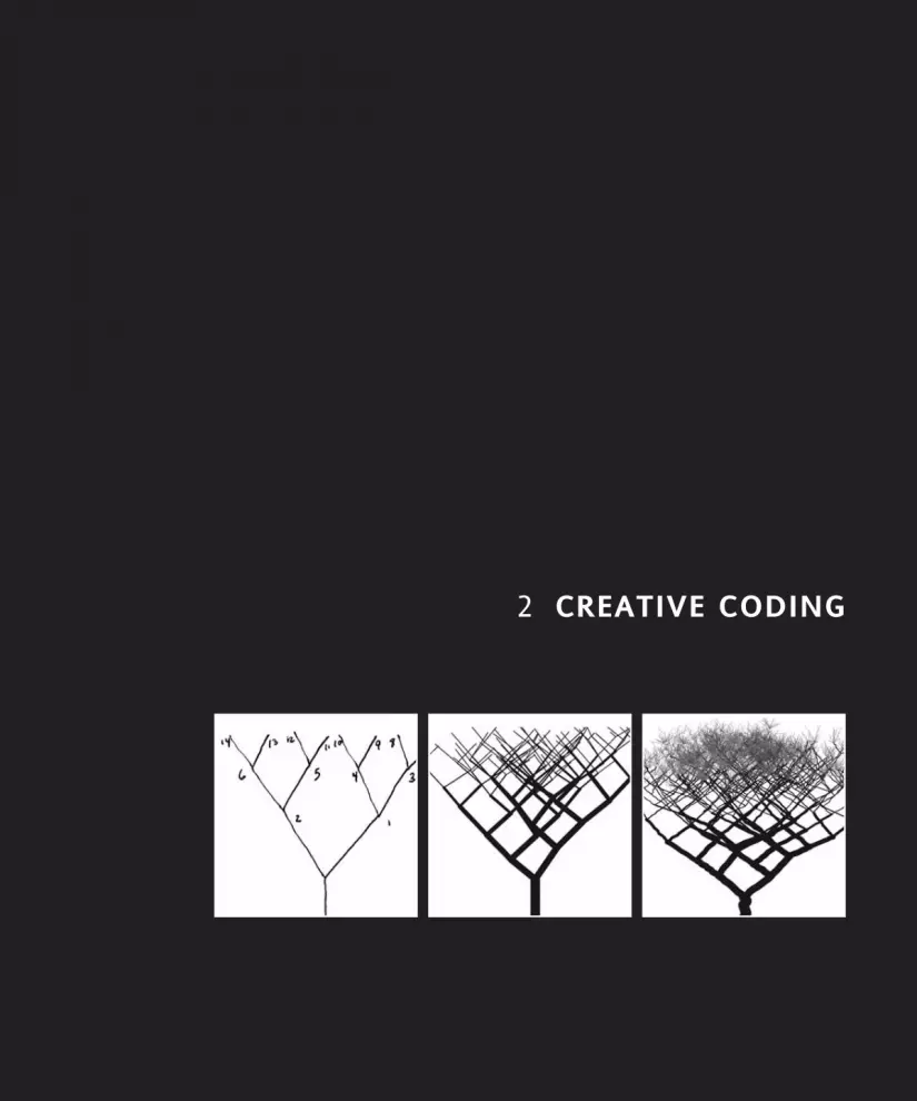
2 CREATIVE CODING
617xCH02.qxd 2/27/07 10:52 AM Page 27
I have a friend, Mark K., who was a web developer who had artistic yearnings (don’t theyall). I met him a number of years ago when he enrolled in a 3D animation course I wasteaching. Mark worked for a sizable, very businessy type company that will remain name-less, doing pretty dull programming. Mostly he was working on legacy code—stuff otherpeople had written—and trying to keep things together with band-aids and string. On topof this, his company was outsourcing most of the interesting development work overseas,and Mark also had the fun job of trying to coordinate video conferences at all hours of thenight (big time difference), while integrating their code (in a programming language/development environment he wasn’t too familiar with) back into the company’s legacyspaghetti (disorganized and poorly structured) code. Is it any surprise Mark was pretty souron coding and dreamed about painting rainbows and unicorns in the Elysian Fields? Well,actually it was more like working in the game industry. We met at the perfect time.
While Mark was losing his passion for coding, I was losing my passion for pretty mucheverything else. I was dreading teaching the 3D course at the time, an area just a few yearsprior I had been passionately involved in. However, my spirits lifted on the first day of classwhen I met Mark. As a first day ice-breaker, I usually have each student tell me a littleabout themselves. When Mark described his programming background, I immediatelyimagined us having these long, intense discussions about the joys and intricacies of coding.Of course this fantasy was shot down quickly as Mark continued to explain his interest ofeventually entering the game or animation industry and his waning interest in program-ming. A little disappointed, I summoned encouragement for his new interest and ambitionand settled in for a long semester. In the end, the semester turned out to be great. Markdiscovered an innate gift and interest in design, and the discussions I originally imaginedhaving with Mark did indeed happen, but of course in a different and actually far moreinteresting way. Mark and I also developed a real friendship that continues to this day.
One of the subjects that Mark and I often discussed was the intuitive vs. analytical natureof coding. Mark had been formally trained as a programmer and thus had developed a“look before you leap” approach to coding that spilled into his other creative work as well.He was trained to analyze a problem, develop a plan, and then implement it. I on the otherhand, trained as a fine artist, was taught to let go of the need to understand everything,and to learn to find structure and meaning in the process. Obviously, the utilitarian aspectsof programming and the pretty much complete lack of utility of painting contributed tothe approaches adopted in our training. At this point, I was mostly coding little graphicsexperiments with ActionScript. I would sit on the couch with the TV on, the laptop burn-ing my legs (PowerBook G4), snacks of course, and tweak code until cool things startedhappening. Eventually one of my convoluted, incomprehensible equations would startyielding something I liked. Then I’d do a “save as” and keep tweaking until I found some-thing else. I was able to hack out tons of art, watch bad reality TV, and still IM Mark dur-ing renderings. Mark was always amazed that I could approach programming that way. Hejust couldn’t see it as an intuitive medium. We eventually tried some collaboration, butwould often get stuck in our planning vs. implementing discussions. In time, though, weboth began to learn from one another. I began planning some stuff before attacking bythe seat of my pants, and Mark began to “throw some dung against the side of the barn.”I really began to see the virtue in Mark’s analytical approach when my projects began toget more complex and I started developing larger applications and reusable classes (whichI’ll cover a bit later). I hope Mark was able to learn from me as well, which seems to be thecase, as he eventually landed an art director’s position, and also has begun to enjoy codingagain—with Processing, of course.
PROCESSING: CREATIVE CODING AND COMPUTATIONAL ART
28
617xCH02.qxd 2/27/07 10:52 AM Page 28

I think what was reinforced for me through my collaboration with Mark was the idea thatto be really effective, you need to approach a problem both analytically and intuitively oreven holistically. It is relatively easy to understand how to approach a painting or evendesign problem intuitively. As children, most of us scribbled with crayons and learned tomake things without much planning. We learned to express ourselves with marks and ges-tures and weren’t too self-conscious about making a mess. Our experiences in math classmay have been quite different, as problems got framed by Boolean logic—the answer iseither true or false. How you were feeling during the process of solving the problem hadlittle bearing on the answer. When a non-expert looks at a design or painting, especially arepresentational image, they believe they can understand it (of course, whether they reallycan is a whole other issue). When that same non-expert looks at a page of computer code,it seems totally inaccessible and very likely overwhelming. They are used to looking at pic-tures and gestures, for which there doesn’t seem to be a right or wrong answer. Looking atcode seems like really hard work, and based on those early experiences in math classes,maybe even scary hard work. You do certainly need to put in some amount of effort tolearn to decipher the code. But the same thing applies to being able to read a painting ordesign. It’s just that many people believe that just because they have eyes, they can intu-itively understand the visual formal language—the underlying pictorial structure—in apainting or design. But seeing, of course—especially seeing critically—involves the brain aswell. Now I could very easily lapse into many pages of the most vitriolic prose about thecurrent plague upon our nation because of rampant visual illiteracy, blah, blah, blah . . .but my editor will surely put the kibosh on that. So let me sum it up by stating that in myhumble opinion it is much, much, harder to learn a foreign language than it is to learn aprogramming language, and having taught both painting and programming, it is much,much, much harder to (really) learn to paint or even draw a figure than it is to gain basicfluency in programming.
If you haven’t thrown the book at the wall yet, a logical next question might be—especiallyif you are totally new to programming—“Exactly how much do I need to know before I canbegin to start hacking out some art on my couch, and of course what snacks do you rec-ommend?” Well, obviously, unlike drawing, you can’t just grab the tool and begin scrib-bling. Well, if you start with some sample code (which Processing responds quite well to),you can, and that is one valid approach to learning to code. However, I think a much moreefficient path, and I guess the main reason for the book, is to quickly (with minimal stress)develop a base coding literacy that will optimize your hack-per-minute efficiency—whichtranslates into making more good art. Regarding snacks, I’m a big fan of Newman’s organicstuff, especially the mint Newman-O’s. (Yuummm!)
For many years, I tried the steal/tweak/pray coding approach, especially with JavaScript.However, there was always this fear and guilt in the back of my mind: the code will break,somebody will find out exactly how little I know, and I really can’t take credit for this.Usually, freelance deadlines beat those feelings back. But using appropriated code that Ididn’t totally understand to make art for myself didn’t feel as good. Also, as a professor Ihate being asked questions I don’t know the answer to. Of course, this happens practicallyevery day when you have bright, talented students—which I’ve mostly been blessed tohave—and are teaching emerging technology. Teaching Flash for many years, I would getasked practically every ActionScript question imaginable, and I eventually got really tiredof BSing my way through half-assed answers. I eventually decided to formally train myselfin programming. I got a mountain of books on programming languages (mostly Java and
CREATIVE CODING
29
2
617xCH02.qxd 2/27/07 10:52 AM Page 29

ActionScript), object-oriented programming, and basic math (mostly algebra and trig), andI took the leap. It was based on this experience that I first got interested in writing a bookon creative coding.
I spent many long, lonely nights with those books, especially the Java API (application pro-gramming interface—basically a description of the language’s rules and tools). Over timeI’ve come to realize that most programming how-to books are excellent for teaching youhow to program if you already have a basic understanding of programming. The Java API,although indispensable to me now, was pretty scary, inscrutable, and downright frustratingback then. When I eventually began teaching entire semester courses on creative pro-gramming, I really learned a lot about how non-technical people learn technical stuff, andmost importantly how to make it engaging. I knew from my own experiences that codewas a powerful creative medium, but how to convince my wide-eyed art students wasanother thing altogether, and I knew most sane people wouldn’t do what I did—tacklingthis scary stuff on their own. I should also point out that besides being obsessive compul-sive, I was a science student prior to being an art student, so I had developed some toler-ance and coping strategies for studying dense, unfriendly stuff. This book is a tribute to allmy coding students who taught me along the way how to be a better teacher and (mostimportantly) what to do to keep them from dropping my classes.
The origin of ProcessingSince around 1945 (or 1834 if you go back to Ada Lovelace’s letter to Charles Babbage),many, many programming languages have been developed—in fact, more, I think thanmost people would guess. Unless you are deep in the computer science world, you maybehave heard of at most five to ten different programming languages. According to asomewhat comprehensive language list at http://people.ku.edu/~nkinners/LangList/Extras/langlist.htm, more than 2,500 languages have been developed. My guess is thatthe number is actually much higher. Interestingly, at the time of this writing, Processingisn’t on the list. This might be due to the list not being properly maintained or becausesome purists might not see Processing as a separate language. What? Well, rest assured, Isent an e-mail telling them all about Processing. But there is a valid argument to be madethat Processing is not technically a language, but more of a programming environment—what is commonly referred to as an IDE, or integrated development environment. I’ll try tomake this argument and then I’ll refute it. I love arguing with myself. However, before I getinto more Processing nuts and bolts, a more conceptual over-the-hood discussion aboutProcessing and its forebear, DBN, will be helpful, or at least (I hope) mildly interesting.
Processing grew out of research in the Aesthetics + Computation group at the MIT MediaLab in around 2001. Prior to that, John Maeda, the group’s famous leader, with the aid ofsome of his students, developed DBN. DBN was a very simple programming language andenvironment, begun in around 1999. Casey Reas and Ben Fry also participated in the devel-opment of DBN. Processing can be thought of as the very advanced, production-gradechild of DBN. DBN was usable on the Web or as a stand-alone application, and was designedto massively simplify the coding process for visual artists. Unlike Processing, DBN didn’thave much application outside of the classroom, as the screen output was limited to about1.5 by 1.5 inches and there was no color. Yet many of the basic processes we expect in aprogramming language were there, including the ability to set and recall values, create
PROCESSING: CREATIVE CODING AND COMPUTATIONAL ART
30
617xCH02.qxd 2/27/07 10:52 AM Page 30

customized commands, and run loops. It even had some basic networking and eventbehavior (mouse and keyboard detection). If you’re interested to learn more, as of thiswriting, the DBN site can still be found at: http://dbn.media.mit.edu/. DBN was devel-oped to simplify the massive complexity involved in graphics programming. Later on in thebook, I will provide some sample code illustrating the minutiae and verbosity of codeneeded to generate the simplest graphics, even in a high-level language like Java. By “high-level,” I mean a language that is supposed to be easier to work in than a low-level lan-guage. You can think of the lowest-level language as zeros and ones. DBN was in a sense areaction to this problem, and it went, some would argue, overboard in addressing it.Processing, having the benefit of standing on the shoulders of DBN, as well as being asecond go-around for Ben and Casey, cleverly addressed this problem by providing a mul-timodal approach, allowing some users to work in a very high-level way—like in DBN—while other codeheads (myself included) could work in pure Java and still others couldwork with a hybrid approach. This totally inspired design, providing choice, is I believewhat makes Processing a very special and cutting-edge tool/environment/language. Today,Processing, free from the confines of the Media Lab, is supported by Ben and Casey, witha growing cadre of devoted (some might say obsessed) “Processors” around the world.
Programming language comparisonsNow for some nuts and bolts. If you get a little lost in this section, don’t panic; it willbecome clearer in time. Also, it is not critical info to get started coding. If you really hateit, just skip it. But I strongly recommend coming back to it eventually. I put it here in thebeginning of the book because I do think it is important.
The argument to be made that Processing is not actually a programming language, butrather a programming environment, is based on the fact that Processing is built on top ofthe Java programming language. Of course, parts of Java itself were created with otherprogramming languages as well (C and C++), so what’s the point? The point is that whenyou run Processing, you are actually running a Java program. Processing allows you to writemuch simpler code than you would need to write if you were working in pure Java. It alsoallows you to structure your code in a function-based (procedural), non–object-orientedstyle. But once you compile your code, the output is converted to Java class files—indistinguishable from any other Java program—and the class files are interpreted withinthe Java Virtual Machine as your program runs. Now don’t freak out! I know I just droppeda bunch of terms you may not be familiar with. We’ll take it slow, and deal with each term,one at a time. Again, my recommendation is to read this stuff and not get too stressed. Ifit’s really bugging you out, skip it and return to it later; you’ll still be a good person.I promise, in time, it will all be clear (or at least clearer).
If you have some prior programming experience with another language, or if you’re think-ing, “Why should I learn Processing instead of another language?” the Processing siteincludes a good comparison and contrast of a competitive set of languages to Processing(http://processing.org/reference/compare/index.html). Of course, I don’t really thinkthese languages compete in any real sense, as each has its own strengths and weaknesses.Additionally, if this coding thing sticks for you, it is very likely that you will learn some ifnot most of these languages in the future. It actually gets pretty easy to learn a new pro-gramming language after you grasp basic programming theory. As I mentioned earlier,
CREATIVE CODING
31
2
617xCH02.qxd 2/27/07 10:52 AM Page 31

learning a programming language is much easier than learning a verbal or natural lan-guage. Now let’s tackle some of the new terms I just threw at you and look at just a littleprocessing code.
First, what does it mean to “structure” your code?
Here is a simple Processing program that draws a black rectangle on a white background;it’s not too ground-breaking, but it is a nice rectangle (see Figure 2-1 for an image of therectangle that the code produces).
size(400, 400);background(255);noStroke();fill(0);rect(width/4, height/4, width/2, height/2);
Figure 2-1. Rectangle created using an unstructured coding approach
A program this simple wouldn’t necessitate structuring your code any further. So, at thispoint, if all you need to make are single squares, you’re done. Congratulations! However,imagine instead of having 5 lines of code, you had 50, or 500, or 5,000? It becomes verydifficult to understand and maintain a program when it reaches a certain scale. There areways of structuring your code, kind of like using paragraphs to organize a chapter, thatmake a large program more manageable. In addition, there are structural ways of simplify-ing your program, reducing redundant lines of code, and ultimately increasing your codingefficiency and possibly the program’s performance (these are all good things).
Function-based (procedural) vs. object-oriented structureThere are a number of ways of structuring your code—I’ll discuss two ways it’s done inProcessing. The first way uses functions (also referred to as procedures, or subroutines—different words essentially describing the same technique). Functions are reusable blocks
PROCESSING: CREATIVE CODING AND COMPUTATIONAL ART
32
617xCH02.qxd 2/27/07 10:52 AM Page 32

of code that work like processing machines, which you call when you need them. Thesecond way uses an object-oriented approach, a far more ambitious and abstract approachthat models a programming problem using concepts from the real world. In object-oriented programming (OOP), the code is divided into smaller (and independent) blocksof code called objects.
Before I describe and contrast each of these approaches in more detail, it is worth statingthat Processing allows you to structure a program using either a function-based, object-oriented, or hybrid approach. In fact, if you want to, you can avoid structure altogether.This amazing flexibility, accommodating different types of coders with varied experiencelevels, is one of the features that makes Processing such a unique environment. Later inthe book, I will go into a much more detailed explanation of this material (I hear yourheart fluttering with delight), but for now I’ll just describe them in very broad strokes.
Let’s go back to the simple five-line program. This program executes from top to bottom.You could test this by moving the fill(0); line below the rect(width/4, height/4,width/2, height/2); line.
size(400, 400);background(255);noStroke();rect(width/4, height/4, width/2, height/2);fill(0);
You wouldn’t see anything if you now ran this program—can you guess why? It’s becausethe color used by the program to draw the rectangle starts out as white, the same coloras the background (255 equals white), and is only changed to black (0 equals black) afterthe rectangle is drawn. So you are actually drawing a white rectangle on a white back-ground. Now, imagine that you have 5,000 lines of code—wouldn’t it be easier to not haveto put every line in an exact sequential order to get the program to run properly? Isn’t thewhole digital thing about not having to be so sequentially linear? Function-based, orprocedural, programming can help solve this problem by breaking a program up intoreusable code structures that you call as you need them. These blocks are called functions(as opposed to objects in OOP); you can think of them as independent processing unitswaiting for action. Functions are explicitly called when they are needed and can optionallybe passed values, which the functions can act upon. Calling a function can be consideredthe entry point of a function. Once called, a function can either end when it completes itsjob, or optionally return values. For example, if I wrote a program to keep attendance inmy classes (something I’ve never done very consistently), I might create a function thatsimply assigned a value of present or absent for each student on a specific date. Then inclass, I could call the function and pass in the value present or absent for each student. Iwouldn’t need the function to return any value. On the other hand, if I wanted to find outwhich students were absent on a specific day, I might create another function that whencalled would return the actual names of the students who were absent.
Let’s make the current rectangle drawing program a little more complicated. Don’t worryabout trying to memorize or even understand the code for now. It is the theory that ismost important. Here’s the program structured using functions:
CREATIVE CODING
33
2
617xCH02.qxd 2/27/07 10:52 AM Page 33

void setup(){size(400, 400);background(255);noStroke();float myColor = getRandomColor();fill(myColor);rect(width/4, height/4, width/2, height/2);
}float getRandomColor(){return random(255);
}
The program still draws a rectangle on the white background, but instead of the rectanglealways being black, the program calculates a random value between white and black forthe fill color of the rectangle. The line return random(255); generates and returns a ran-dom number between 0 and 255. 0 equals black and 255 equals white, and anything inbetween equals a variation of gray. You’ll notice the program now has these strange brack-ets,{ (open) and } (closed). These are called curly braces, and they are used to group thelines of code needed by the function to do its job. You’ll also notice that the program isbroken into two groups of code: void setup(){...} and float getRandomColor(){...}.These groups are both functions. The lines void setup(){...} and floatgetRandomColor(){...} are the function declarations. It is a good idea to use a verb inthe name to describe what the function does. That way, it is easy to understand what thatfunction’s job is when reviewing the code. Also, a function is followed by open and closedparentheses. This is the place where any arguments (values) the function will need to doits job are included—commonly referred to as “passing arguments.” Even if no argumentsare required, as in the preceding case, you still need to include the parentheses.
There is another very common programming structure called a variable, which I’ll discussin detail a little later in the book. A variable is simply a location in memory that will hold apiece of data. For instance, in the left part of the expression float myColor =getRandomColor();, float myColor is a variable, to which a numeric value can beassigned. The word “float” just specifies the type of numeric value the variable can hold.
The line float myColor = getRandomColor(); is a function call. Actually, the right part ofthe expression, getRandomColor();, is the function call, and the left part of the expression(float myColor =) simply assigns the value that the function call returns to the myColorvariable. Here’s where things get a little interesting. When the getRandomColor() functionis called, it takes over—before the line below the function call (fill(myColor);) is dealtwith, the code inside the actual getRandomColor() function is run. Only when the functioncalled finishes will the code below the function call be run. Inside the getRandomColor()function, one of Processing’s built-in functions, random(), is called. Once the random()function does its job, it returns a number back to where the getRandomColor() functionwas called from, and this returned value is assigned to the variable float myColor. I real-ize this may seem a bit overwhelming if this is your first time dealing with coding; I prom-ise it will make (more) sense over time.
OOP was developed later than function-based or procedural programming, and wasdesigned to try to improve on some of procedural programming’s perceived limitations.In a general sense, OOP was designed to allow the types of modules that functions
PROCESSING: CREATIVE CODING AND COMPUTATIONAL ART
34
617xCH02.qxd 2/27/07 10:52 AM Page 34

introduced to become larger, more complex, and more independent entities. OOP facili-tates code reuse—which will become more important as you get more experienced—andenforces certain programming rules. OOP is a much more complex approach to program-ming that delves into very interesting but quite challenging abstractions. I will cover OOPin Chapter 8, although I include a brief overview of it in the next chapter, which focuses oncode grammar. OOP is such a big subject that it would be worthwhile to devote an entirebook to creative OOP with processing—maybe if I’m still standing when I’m done writingthis one . . .
If you’re interested, here is a Processing OOP version of the little rectangle program, withsome comments—the descriptions following the two forward slashes (//). I am not goingto do a full analysis of the program here, as I’ll be covering these concepts in painstakingdetail later in the book.
// Processing Object-Oriented approach: Create a rectanglevoid setup(){// set display window to 400 x 400size(400, 400);// set background color to light graybackground(225);
//instantiate a MyRect object and assign it to the reference !variable rectangle1
MyRect rectangle1 = new MyRect(width/8, height/8, width/4, !height/4, 200, -1);
/* call drawRect() method using MyRect object reference, rectangle1calls the method using dot syntax (literallythe period between the object and the method call).*/
rectangle1.drawRect();}
// MyRect class definitionclass MyRect {
// public instance fields - each MyRect object will have// their own set of these propertiesfloat x, y, wdth, ht;int fillCol, strokeCol;
/*constructor - called when the object is instantiated, using the newoperator. the parameter list between the parentheses needs to match the argument list in the instantiation call */MyRect(float x, float y, float wdth, float ht, int fillCol, !int strokeCol){// initialize instance fields - assignment happens form// right to left, e.g. the value of x is assigned to the // instance property this.xthis.x = x;
CREATIVE CODING
35
2
617xCH02.qxd 2/27/07 10:52 AM Page 35

this.y = y;this.wdth = wdth;this.ht = ht;this.fillCol = fillCol;
/* check for stroke - if the last argument passed to theconstructor is not -1 then use that value to set the stroke color. If it is -1, don't draw a stroke */
if (strokeCol!=-1){this.strokeCol = strokeCol;stroke(strokeCol);
}else {noStroke();
}}
//drawRect methodvoid drawRect(){//assign fill colorfill(fillCol);// draw rectanglerect(x, y, wdth, ht);
}}
The other terms I threw at you earlier were “class files,” “compile,” “interpret,” and “JavaVirtual Machine,” which I’ll define as I introduce Java and describe Processing’s specialrelationship to it.
JavaI want to cover a little of Java’s history (sorry), but I think you may find it somewhat inter-esting, especially as a lesson in the virtue of happy mistakes. I actually cover happy codingmistakes a little later on as well. Java’s history is also relevant in regard to a deeper under-standing of Processing. Have I convinced you? Hope so.
Java, originally named Oak, was developed in the early 1990s as a language to be used toprogram devices other than personal computers—things like microwave ovens withembedded processors—not terribly sexy stuff, but as you’ll see, pretty visionary. However,appliance manufacturers didn’t embrace the idea. So to save face, the Sun engineers wentback to their drawing boards and came up with a plan to remarket Oak as a language tocontrol “set-top boxes” for interactive TV. But alas, the cable companies passed on that ideaas well. Things were not looking good for Oak. To make matters even worse, it was discov-ered that the name “Oak” had already been trademarked by another technology company.Before I tell you how Java was reborn out of this very inauspicious beginning, let me explainthe basic problem the Sun engineers were trying to address in the design of Oak in the firstplace. Then you can try to guess (if it is not already obvious) what saved Java.
PROCESSING: CREATIVE CODING AND COMPUTATIONAL ART
36
617xCH02.qxd 2/27/07 10:52 AM Page 36

Without getting too geeky, the main objective in the design of Oak was to develop a rela-tively simple-to-program, high-level, universal programming language. The really key wordhere is “universal.” A proprietary technology (and a refusal by companies to respect andadhere to standards) creates a difficult landscape to work in. This problem is not limited tothe computer industry. A number of years ago my wife and I invested in a water filter sys-tem that attaches directly to our kitchen faucet. Over the years we’ve moved a lot, drag-ging our filter with us. In almost every new home, we’ve had to contact the filter companyto request yet another odd-sized adapter (we’ve got a quite a collection by now). Lack ofstandardization has up until recently been especially frustrating and difficult for webdesigners, who were forced to develop multiple sites, limit design concepts, and createcrazy workarounds to ensure that their sites worked across all the different web browsers(this is no longer so much of a problem because of the advent of web standards, betterdevelopment practices, and better and more consistent support for those standards acrossbrowsers).
One of the benefits of a program like Flash is a universal Flash player that ensures consis-tent content delivery across different platforms (operating systems and web browsers).The history of Flash, originally called FutureSplash Animator, arguably would have beenquite different had Java not a few years earlier pioneered the concept of a portable,universal language.
So the emergence of the Internet saved Java. Java’s now well-known slogan, “Write once,run anywhere,” turned out to be the perfect strategy for the Internet. And by 1996, Javawas also embedded in Netscape’s browser, ushering in a revolution in online multimedia-based content and development. Interestingly, in the ten years since this development,Flash has far surpassed Java as the online multimedia-based (front-end) content tool ofchoice, and Java has moved to the back end of the Web—to the server side. Java is alsowidely used on mobile and wireless devices, such as PDAs and cell phones. With the devel-opment of Processing, Java is again being used for online content creation. So arguably,Processing has saved (or at least resurrected) the Java applet. Although unlike Flash, whichis used to enhance/develop entire websites, Processing (currently) is being used primarilyfor aesthetic exploration. Of course, as more Processing tools and code libraries are devel-oped, this could change. OK, so that’s a nice story, but how do Java and Processing work?
Java is considered both a compiled and interpreted language. Unfortunately, the terms“compiled” and “interpreted” don’t quite mean the same thing in programming as in gen-eral parlance. To compile, in computer-speak, is to convert a (usually high-level) program-ming language into something lower level. Remember, a computer likes zeros and ones(the lowest-level language), but most people find it frustrating to communicate in binarycode. It is easier to write programs in the same natural language we speak (the highest-level language), but a spoken language is extremely complex and would demand tons ofprocessing to be able to interpret it. Therefore, in the design of a programming language,there is a trade-off between ease of use and performance.
Java was designed with this trade-off in mind. Sun’s Java compiler, javac (Processing actu-ally uses a similar open source compiler, developed by IBM, called jikes), converts a pro-grammer’s code (the stuff we write) into a middle-level language called bytecode (that thecompiler writes). This bytecode (also known as class files) is universal, meaning that I cantake my class files compiled on my Mac and run them on a Windows machine, as long asthe Windows machine has a Java Virtual Machine (JVM). As most operating systems and
CREATIVE CODING
37
2
617xCH02.qxd 2/27/07 10:52 AM Page 37

browsers have a JVM, I can use my class files in any of these environments, regardless ofwhere they were written. Thus, you can see the power of Java’s “Write once, run any-where” strategy.
In Java’s early days, it was considerably slower than non-interpreted languages like C orC++, which don’t use a middle compilation state (the bytecode). These languages compiledirectly to machine code specific to the native underlying system. Thus, these languagesare highly efficient, but not easily portable. If you write a program in C++ on a Mac, it willonly run on a Mac. You have to literally go in and change some of your code to create asecond version of your program (referred to as porting your program) if you want it to runon a different platform. Today, based on certain advances in compilers, such as “just-in-time” compilers (in which some of the Java bytecode is compiled to native machinelanguage instructions during runtime), Java’s speed is comparable to lower-level, non-interpreted languages like C and C++. This gap continues to narrow, or become insignifi-cant, as computers continue to get faster. So Java’s strategy seems to be really paying off.
Processing has all the benefits of Java with a much simpler and optimized environment forcreative coding. As an example, following is the original five-line rectangle drawing pro-gram written in Processing. I’ve also written the same program as a Java applet.
Here’s the original Processing program:
size(400, 400);background(255);noStroke();fill(0);rect(width/4, height/4, width/2, height/2);
Here’s the same program as a Java applet:
import java.awt.*;import java.applet.*;
public class MyStage2 extends Applet{public void init(){setSize(new Dimension(400, 400));setBackground(Color.white);
}public void paint(Graphics g) {g.setColor(Color.black);g.fillRect(getSize().width/4, getSize().height/4, !getSize().height/2, getSize().height/2);
}}
The Java applet requires about twice as much code as the Processing sketch. However, asyou write more complex programs in Processing, the number of required lines of code towrite the same program in pure Java begins to increase exponentially. So if Processing isessentially Java, how does it do the same thing with less code? It does it by using a softwareframework that does a lot of the extra (non-creatively oriented) work under the hood,leaving you to just concentrate on the fun stuff.
PROCESSING: CREATIVE CODING AND COMPUTATIONAL ART
38
617xCH02.qxd 2/27/07 10:52 AM Page 38

A framework is just a concept for bundling precompiled code together for use in devel-oping a related family of programs. From a programmer’s standpoint, a good frameworkallows you to write less code and focus more on the higher-level concerns of your program.Java relies on many frameworks. For example, Java’s Collections framework allows differ-ent types of groupings of objects (collections) to be manipulated in a uniform way, and, asSun says, “independently of the details of their representation.” This is a huge advantageto a coder, who now only has to learn one approach (a single pattern) to getting or settinga value within a collection of objects, even though internally these collections may usevery different implementations. The Processing framework does a similar thing, but in thearea of creating and manipulating graphics and images. Graphics programming is complex,and using pure Java involves ascending a pretty steep learning curve. In addition, afterlearning how to create some graphics (shapes and text), you would still need to learn awhole new set of procedures for working with images, not to mention video, animation,and so on. Using the Processing framework, these disparate and complex operations arestandardized into a uniform and simplified set of commands.
Procedural OOP (“poop”) approachI suspect by now, if you’ve stuck through this chapter, you’re in need of a little diversion,so a short story might be refreshing. A number of years ago I was preparing for a show ofmy paintings. I was very excited about the show, as I was only a few years out of gradschool and had this romantic vision of being discovered, and picked up by a major NewYork gallery. The fact that my show (actually a two-person show with my friend David) wasat a small cooperative gallery in Piermont, New York, didn’t seem to have any effect on myfantasy. In preparing for the show, I stretched up a number of large, impressive lookingcanvases on which to create my “serious” work. Besides preparing for my show, I also hada brain-numbing job doing mostly print production work for an aesthetically bankrupt(though not at all financially bankrupt) corporation. My one fun indulgence was aThursday night drawing group I frequented in Manhattan.
When I first moved to New York City, I looked up an old professor who invited me to aweekly drawing group at his studio. I was of course thrilled and went to my first sessionexpecting to bask in all the intense aura of professional, established New York artists atwork, but instead found a party-like atmosphere with free-flowing wine, loud music, andcontinuous conversation. In time, I became quite accustomed to this new approach andhad a great time listening to the older artists tell stories about the good old days, and ofcourse we did make art.
So each week I would go to the drawing group, crank out a bunch of work, come back tomy studio, and pile the work in the corner. During the days, when I wasn’t sloggingthrough Quark at the mind-numbing job, I painted my “serious work.” This went on fornearly a year, until I began final preparations for my show. When it got down to selectingthe actual paintings to put in the show, I had a major revelation (it actually felt more likea kick in the head). My serious work, well, kind of sucked. It was self-conscious and forced.I was pretty desperate and had no time to create new work, so I went to the corner withmy “non-serious” work piled high from the Thursday night drawing parties and startedrifling through the pile. I was shocked—the work was really interesting and fresh, but alsoaccomplished in its own way. The work had spontaneity and energy, but it also had
CREATIVE CODING
39
2
617xCH02.qxd 2/27/07 10:52 AM Page 39

structure and clarity. The “serious” day painting that I thought was my real work was actu-ally something else altogether. In retrospect, although the work was self-conscious andforced, the discipline of doing the serious painting contributed to my skills and technique,allowing me to let go on Thursday night to really express myself. It was this combination ofdiscipline and freedom that I attribute to the quality of the work. I ended up only puttingthe Thursday night work in the show, and got a very positive response. Of course I didn’tget famous, but I certainly kicked butt in Piermont.
So what the heck does that story have to do with Processing? Well, when it comes to writ-ing creative software, there are a number of ways to approach it. There is the “serious”way and there is the Thursday night party way. It is not so much a specific set of techniquesI’m talking about, but rather an attitude. Some programming languages and environmentsdemand a highly structured and rigid approach that doesn’t favor spontaneous expressiveshifts. OOP, which is a beautiful construct that I will go into later in the book, requiresplanning and a well-thought-out plan; Without such a plan, a “by the seat of your pants”OOP approach can lead to piles and piles of code and excess complexity, taking you awayfrom self-expression and burying you in pure digital craft, or worse—damage control. Theother extreme, pure gut hacking of unstructured spaghetti code, can yield fast effects andlittle teasers, but it becomes overwhelmingly difficult to carry a creative impulse throughto a more realized form. So there needs to be a middle way, combining structure with fastprototyping capabilities. This yin/yang approach is possible in Processing, which provides afast, loose, procedural coding environment with a highly structured and powerful object-oriented backbone. That is not to say there aren’t pitfalls to working in such a flexibleenvironment, in which it’s easy to develop nasty hacking habits. My recommendation, andthe way I’ve structured the upcoming tutorial sections in the book, is to begin coding withpassion. Don’t let the fear of doing it right or learning everything first get in the way ofexpressing yourself, but at the same time, study the language (first Processing and theneventually Java) and OOP; it will ultimately empower you to create larger, more expressiveworks.
Algorithms aren’t as scary as they sound1. Buy a new copy of Processing: Creative Coding and Computational Art.
2. Open the book to page 1.
3. Begin reading at the top of page 1.
4. Stop reading at the bottom of the last page of the book.
5. Write a glowing review of the book on Amazon.com.
6. Go to step 1.
These six steps constitute an algorithm. They are not a computer program—they are justspecific directions on how to achieve something. The term algorithm comes from AbuAbdullah Muhammad bin Musa al-Khwarizmi (referred to just as al-Khwarizmi), a Persiansupergenius (with a really long name) from the early part of the ninth century. We get theword algorithm from the al-Khwarizmi part of his name. al-Khwarizmi worked nearBaghdad as a scientist, mathematician, astronomer/astrologer, and author. He is also com-monly referred to as the father of algebra. You may have first been introduced to the word
PROCESSING: CREATIVE CODING AND COMPUTATIONAL ART
40
617xCH02.qxd 2/27/07 10:52 AM Page 40

algorithm in a math class in high school, but you may have been daydreaming at the time(or, if you’re anything like me, drawing a less-than-flattering picture of your math teacher).Algorithms are fundamental to mathematics, but they are also essential to pretty muchany other planned activity. If you go to Google and type define:algorithm, as of this writ-ing, 28 definitions come up. One definition I like in particular, from http://images.rbs.org/appendices/d_glossary_geometric.shtml, is “A step-by-step procedure used forsolving a problem.” I like this definition because it is so incredibly simple and universal,and can be applied to practically any problem. The only thing I might add to the definitionis the limit on the number of steps. My new definition is “A finite step-by-step procedureused for solving a problem.” When you’re dealing with programming—or really, any task—an infinite number of steps is almost always a bad thing. For example, in the precedingalgorithm I wrote, experienced coders probably saw a major logic problem; the algorithmnever ends. Intellectually this might be an interesting idea, like a hall of mirrors endlesslyreflecting one another, but in programming we call this an infinite loop. Loops are centralto programming, but we usually want them to end when some condition is met. Forexample:
1. Buy a new copy of Processing: Creative Coding and Computational Art.
2. Open the book to page 1.
3. Begin reading at the top of page 1.
4. Stop reading at the bottom of the last page of the book.
5. Write a glowing review of the book on Amazon.com.
6. If Ira’s still not a millionaire, go to step 1.
7. Stop following this algorithm (and thank you)!
The logic in the algorithm will no longer generate an infinite loop. Instead, at step 6, onlyif the condition is not met (alas, I’m still not a millionaire) does the algorithm repeat. Buteventually the condition will be met, step 6 will be skipped, and step 7 will end the loop.Unless there is some specific direction to go somewhere else (e.g., go to step 1), the pro-gram keeps executing from top to bottom. This is why the program falls through step 6when the condition is no longer met and executes line 7, ending the loop.
Computers are inherently dumb machines. They are super-quick at processing data andhave awesome memories, but they have no innate intelligence. For example, if I asked acomputer to hold a 1,000-pound weight over its head (just assume computers have arms),it would eventually destroy itself by dropping the weight on its head when its arms gaveout. Why? Because computers are perfect literalists; they do only and exactly as they aretold, without any assumption, reflection, or self-awareness. Unless I instructed the com-puter to put the weight down when it felt its arms getting tired, it wouldn’t do it. One ofthe difficulties in learning to code is not that we have to think so brilliantly, but rather thatwe have to think so mind-numbingly literally—without the benefit of emotion, assump-tion, or intuition. For example, if I want to ensure that you will continue reading this book,I could tell you that you must keep reading this book. However, because people are intel-ligent and not robotic literalists, the majority of you will likely tell me to go to hell.Generally speaking, if we want human beings to do something, we need to make an appealwith a more complex strategy, taking into account feelings, social conventions, personalhistory, favorite baked goods, and so forth.
CREATIVE CODING
41
2
617xCH02.qxd 2/27/07 10:52 AM Page 41

Humans are excellent at intuiting. We can meet someone for the first time and within acouple of minutes build a complex initial profile of the person; not that all these assump-tions hold up—but it’s amazing, with so little data, that any do. We seem to be able toremember subtle general patterns of behavior that let us build composite types.Psychologists have named this organizing function gestalt. Gestalt is also commonlydefined as the sum of the parts being greater than the individual parts. For example, whenyou show someone a picture of Elvis, they don’t think “two eyes, a nose, lips, sideburns,sequins, etc.” They don’t even think “man” or “human being”—they think, “It’s Elvis!” Thegestalt allows our minds to generalize object-oriented models based on our memories andsensory data. The gestalt makes us highly efficient at processing vast amounts of complexinformation without going insane. Imagine if we were constantly aware of all the sensorydata surrounding us? However, this amazing organizing ability we have can also causemajor problems when we think our limited mental models reflect all of reality. Teachingdrawing for many years, I felt my hardest job was convincing the students to let go of theway they thought they saw the world, to be able to learn to see it again freshly and expandtheir perceptual paradigm. When people first start out learning to program, they typicallymake some common intuitive assumptions because of the gestalt. These types of assump-tions, which work more or less in the real world, fail miserably when applied to program-ming. Computers innately lack an internal gestalt to discern the whole from the parts.They are essentially just dumb (although ridiculously powerful) calculators. If computershave any intelligence at all, it is at the software level. Software—operating systems, pro-gramming languages, and applications—to some degree create a gestalt-like reality in thecomputer, the so-called spirit in the machine. Thus, perhaps the passion people feel fortheir machines is really a connection to the spirit imbued within the machine (the soft-ware)—which of course is the human presence.
Here’s a concrete example that illustrates how our sophisticated brains can get us intotrouble when we first start writing code. An exercise I always cover early in my creativecoding class is how to generate a simple moving object programmatically (meaning usingcode). The problem is pretty simple: Create a small rectangle—we’ll name her “recty”(she’s a female polygon). Make recty move around the screen and have her bounce off theedges of the frame, never letting any part of her go out the frame.
The first challenge students generally encounter in this problem if they have no program-ming experience is simply moving recty. For this example, let’s assume that recty is alreadyon the screen in a frame and has an x property. This means that recty’s x position (her hor-izontal position) on the frame can be set and retrieved by using her x property. Alsoassume that recty’s registration point—a point or pixel on recty that the x property ismeasured from—is in her top-left corner, and there is also a variable named speed thatcontrols how fast recty moves. I’ll assign a value of 3 to the speed variable using theexpression speed = 3, and I’ll also start a loop running that continues to update the frame(and recty’s position). I’ll be covering all this stuff in more detail later on, so it’s OK to bea little out of breath at this point—but just avoid operating any heavy machinery.
To move recty, most new coders try this first: recty.x = speed, which I think makes per-fect sense because they’re assigning speed to recty’s x property. Unfortunately, this expres-sion doesn’t get recty moving; although something else happens—recty gets moved to theleft edge of the screen (to 3 pixels to the right of the left edge of the frame) and staysthere, because recty.x = speed doesn’t increment recty’s x position by speed, but ratherassigns the value of speed (which is 3) to recty’s x position—putting her at that point in the
PROCESSING: CREATIVE CODING AND COMPUTATIONAL ART
42
617xCH02.qxd 2/27/07 10:52 AM Page 42
frame. The loop keeps running and keeps assigning 3 to recty.x, so she doesn’t move(poor recty), even though the frame is being refreshed continuously. So why do people dothis (besides just to annoy their teachers)? I think it’s because it is so easy for us to under-stand how to move that we don’t waste any brain cells thinking about it.
Let’s imagine you and I were standing across a room from one another and I’d like you tocome join me on my side of the room. More than likely, I’d just say “please come overhere.” Your brain would fill in all the details on how to pull this off, which it would thencommunicate to your body and you’d begin walking across the room, most likely in adirect path toward me. Even though I didn’t tell you a rate or direction to move, you’dknow exactly what to do. Of course, my one-year-old daughter would probably notrespond to the same verbal cue. However, if I held up a shiny object from across the room,she’d likely begin crawling over to me, also in a straight path no less. One of our challengesin programming is thinking beneath our intelligence. Although moving across a room mayseem like a really simple task, there are a tremendous number of assumptions and calcu-lations we make to achieve it, not to mention some pretty insane physics. When we modeleven simple behavior on the computer, we need to account for these assumptions—whichis difficult. The correct solution to the movement problem is the following expression:
recty.x = recty.x + speed
Now this expression often looks a little confusing to people in the beginning. Why wouldsomething be equal to itself? It seems illogical. First of all, in programming, the symbol =doesn’t mean equals, but rather assignment. The symbol == means equals—I know thisseems weird. It might help if I write in English what’s going on in the expression recty.x =recty.x + speed: “Add the value of the variable speed to recty’s current x property, thenassign that value back to recty’s x property, and then do it again and again. . .” Thus, aftereach loop cycle, recty’s x property will increment by 3. By writing the logic out as an algo-rithm, you can better understand what’s happening. In this case, recty.x keeps increasingeach loop cycle of the program, moving her across the screen. Will recty stop when shehits the end of the frame? Nope, we didn’t tell her to. In fact, recty would continue mov-ing until we quit the program, but of course you won’t see her, because she’s out of theframe. If this is still unclear, don’t worry at all. This is difficult stuff to begin to get yourhead around. Another trick to help you understand this stuff is to do the calculations man-ually. For example
Remember speed equals 3.
Start recty.x out at 0.
First, loop recty.x = recty.x +speed.
Now recty.x equals 3.
Second, loop recty.x = recty.x +speed.
Now, recty.x equals 6.
Third, loop recty.x = recty.x +speed.
Now recty.x equals 9.
See the pattern.
CREATIVE CODING
43
2
617xCH02.qxd 2/27/07 10:52 AM Page 43

I hope that helps; it will come in time if it’s still a bit fuzzy. If you’re anything like me, It justtakes some time to restart the brain after years of turpentine exposure and bad TV. Whenyou get stuck on a programming problem, it really does help to write out a simple algo-rithm. Later on, when you begin cranking out thousands of lines of dense code, creatingalgorithmic roadmaps before you start coding might even eventually begin to feel likeconceptual brainstorming or preliminary sketching—of course, by then you will also be acertifiable geek.
Happy coding mistakesAfter my diatribe about algorithms, how can a coding mistake be seen as happy? Well, Idon’t mean “computer bug” when I write “mistake.” A bug is usually not happy. Bugs arewhen stuff happens that is not very interesting and usually annoying. Bugs are the things insoftware—such as missing semicolons, misspelled variable names, or infinite loops—thatcan drive you insane and make you try to physically impale your keyboard. Happy codingmistakes, on the other hand, are nonfatal things that happen, often revealing unforeseenpossibilities. As a painter, it took me a long time to be comfortable with my mistakes(which were many). I wanted to control the paint—which of course is pretty much impos-sible. In time, I began to realize that the so-called mistakes I was making were often thebest parts of the paintings. This phenomenon occurs in all creative pursuits, as somehowour unconscious mind seems to assert itself when we least expect it. Arguably, this is alsowhere our inspiration lies. I think more experienced artists just learn how to better utilizethis capability as well as gain the ability to more selectively recognize the happy accidentsfrom the bugs. Coding is a creative process, and thus code art can benefit from thesehappy mistakes. However, because the process of coding involves many more rigid rulesthan painting, it is not as easy to understand the concept of happy coding mistakes. Inaddition, when starting out coding, it is easy to get caught up in the technical aspects orcraft of coding and lose sight of its power as an expressive medium.
There is a macho aspect to coding, as well as to painting. You begin to feel powerful andcapable of describing all kinds of interesting behaviors; plus, you have access to a secretlanguage that most people don’t understand. Coding can become like a giant, multidi-mensional crossword puzzle, and you can easily get consumed in these really dense,abstract worlds—losing site of expressive possibilities or what you need to say (in an artis-tic sense). You need craft in coding; the more mastery you have of your medium, the widerthe scope or range of your work. You also need a creative vision; without it, coding canbecome an analytical quagmire. I can’t say that I always navigate clear of the quagmiremyself, as I often get caught in trying to solve these endless, albeit interesting, technicalproblems. But when I let myself play with the code and let things happen that are notcompletely in my control, I often have more fun and even experience the same kind of(warning; new-agey phrase coming) transcendent feeling I get when I am in the flow ofpainting. I also think the work is more original and expressive. Ultimately, I think it is aboutfinding flow in the coding process that takes you to new places and allows you to turnyour so-called mistakes into new and fertile investigations.
OK, let’s assume you buy some of this; a logical question for a new coder to ask is “Howdo you begin to find or embrace happy coding mistakes when you don’t even know thefundamentals (or basic craft) of programming?” I think the answer is to always try to find
PROCESSING: CREATIVE CODING AND COMPUTATIONAL ART
44
617xCH02.qxd 2/27/07 10:52 AM Page 44

the time to play at whatever level you are at. This is a really important approach thatteachers are sometimes lousy at implementing. It is easy to get caught up in teaching thepursuit of mastery, focusing on achievement goals for students and checking off the req-uisite material covered. The school system reinforces this approach with standardized test-ing, creating crammers and compartmentalizers who separate work and play, craft fromart. Is it any wonder that many of us (especially creative types) felt bored and frustrated inthe traditional classroom, especially in subjects that required methodical drilling or rotememorization (like math)? Sadly, as we get older, we eventually label these subjects as theproblem, not the non-integrated teaching approaches. My experience in the classroom hasbeen that I find most people receptive to learning anything when it’s taught effectively.And my vision of effective teaching always involves finding a way of integrating aspects ofplay and work into the learning process. Before I launch into yet another whiny soliloquy,I’ll sum it up with the following: real code art (whatever the heck that means) can bemade at any level—by a newbie coder learning the basics or a seventh-degree Java blackbelt—and happy coding mistakes help us see the expressive possibilities at whatever levelwe are at.
Before I end this chapter, I think it might be helpful to illustrate this point with a shortexample of how I approach happy coding mistakes in my own process.
Algorithmic treeI used to paint a lot of trees. Originally, I painted the entire landscape, but gradually overtime, I found myself zooming in closer on the trees, until one summer, I painted an entireseries of large paintings based on part of one tree. It is interesting watching your neigh-bors’ reactions as you spend more and more time standing in your backyard, staring up atthe same tree.
So in honor of my favorite tree, I thought I’d illustrate some creative coding by generatinga tree with code. Let me also preface this by saying that you shouldn’t try to follow thiscode unless you already know how to program; it may seem totally overwhelming. Mymain point here is to reveal my creative process, not to teach the code; the rest of thebook is for that. Feel free to run this sketch and make changes to the code to see whathappens. If you get any really cool results, I hope you’ll e-mail me some screenshots.
In considering the problem, I decided to think about trees some and to break the problemdown into simple parts. In a moment of brilliant clarity, I concluded that trees have atrunk, branches, and leaves. OK, I know I can probably make a trunk (think straight verti-cal line). Branches could be a little harder, and leaves, well, probably too hard (actually toomuch work). Branches, I concluded, could be simplified as a thin trunk, splitting off toanother series of thinner trunks, splitting off to another series of thinner trunks, and so on.Thus, it seemed branches could be made from a single branch machine, in a fractal pro-gression (huh?). By fractal progression, I mean the branches are self-similar and repeat.Each branch’s ending point is a starting point for more branches, with a decreasing scale.Thus, the tree thickness decreases from trunk to branch—which seemed pretty consistentwith real trees. I decided to put the leaves on hold for now. I was ready for a little sketchof my branch plan (see Figure 2-2).
CREATIVE CODING
45
2
617xCH02.qxd 2/27/07 10:52 AM Page 45

Figure 2-2. Initial schematic sketch of tree branching structure. The numbers represent the algorithmic branching order.
The drawing is a basic symmetrical tree structure in a purely schematic form. Betweeneach branch is a node. I added some numbers for the nodes to think a little how the com-puter would sequentially draw the structure. So I was now ready for an algorithm thatwould help me write code to generate the tree form. Again, the tree trunk was just goingto be a line, so I figured I’d come back to it. Here’s the branching algorithm:
1. Draw two or more opposing diagonal branches from the top of the trunk.
2. At the ends of these branches, continue adding two or more opposing diagonal,slightly thinner branches.
3. Go back to step two until a specific limit is reached.
The algorithm seemed simple enough, and I noticed that it could possibly loop back onitself—or even call itself. We call such an approach in programming recursion, where afunction calls itself. Recursion is a somewhat advanced concept, even though it is not thatdifficult to implement. Recursion will lead to an infinite loop (a bad thing) unless someexplicit limit is set. For example, I could tell the program to run until one of the branchestouched the top of the frame, or until there are 700 branches on the tree, and so on.
After a couple of well-placed slaps to my head, I finally got the basic branching code writ-ten (please note that this code fragment will not run in Processing yet):
void branch(Point2D.Float[] pts){int stemCount=2;if (counter2<branchLimit){
for (int j=0; j<stemCount; j++){line(pts[counter2].x, pts[counter2].y, !pts[counter2].x+xg, pts[counter2].y-yg);
pts[counter+1] = new Point2D.Float(pts[counter2].x+xg, !
PROCESSING: CREATIVE CODING AND COMPUTATIONAL ART
46
617xCH02.qxd 2/27/07 10:52 AM Page 46

pts[counter2].y-yg);xg*=-1;
counter++;}counter2++;branch(pts);}
}
I don’t want to spend too much time on the code here, as lots of coding is coming up insubsequent chapters. I’ll just give a quick overview of how the function works. If you feeloverwhelmed at any point, just skip the code parts. In Chapter 3, I’ll begin with a verygentle introduction to the fundamentals of coding, so don’t panic. What I’m really inter-ested in illustrating is a creative process using code.
The branch function expects an array, of type Point2D.Float, as an argument (the stuffbetween the parentheses at the top of the function). An array just holds a bunch of values,as opposed to a variable, which only holds a single value. I chose to use Java’s Point2D.Floatclass because it has built-in x and y properties and can handle real numbers (as opposedto only integers). The stemCount variable controls how many branches each subsequentbranch gets. I hard-coded it to 2 just for now. The for loop draws the diagonal lines andupdates the pts array with the new branch locations. The variable xg controls whether thebranches lean left or right. By continuously multiplying xg by –1, it keeps togglingthe branches from right to left—not terribly organic, but efficient. The counters keeptrack of stuff, and then I recursively call the same function, passing in the updated ptsarray. At this point, you are probably either like “Cool, that makes sense,” or “Is it too lateto return this book? This guy is nuts!” Well, I may be nuts, but I don’t expect most ofyou to be able to follow this code. However, hearing some of these terms over and overwill help with the “stick in your brain” part. What is really much more important and inter-esting is how to turn this cold schematic diagram into a tree (see Figure 2-3).
Figure 2-3. Initial code implementation of the branching algorithm
CREATIVE CODING
47
2
617xCH02.qxd 2/27/07 10:52 AM Page 47

After being somewhat satisfied with the branch algorithm, I started playing with the code.The first thing I did was add some random functions that moved the branches in slightlydifferent places. The random functions contribute to the happy mistakes. Sometimes, I’llput in values that are outside of a reasonable range just to see what happens. Already thisstarted looking better (see Figure 2-4).
Figure 2-4. Randomness added to the branch structure
Next, I added thickness (using the radius variable) to give the tree some form. Beginningwith a larger radius value—not really a radius, but more like thickness—for the trunk, Idecremented the radius variable slowly each time the function ran, letting the branchesslowly attenuate. This began looking a little more tree-like, as you can see in Figure 2-5.
Figure 2-5. Stroke weight variation begins to create a more realistic-looking tree.
PROCESSING: CREATIVE CODING AND COMPUTATIONAL ART
48
617xCH02.qxd 2/27/07 10:52 AM Page 48

The overall movement was good, but the tree seemed too stiff, so I wrote a little redraw-ing function that added some waviness to the main trunk, and I set this up as a randomvalue. Using randomness is really helpful for generating organic-esque type effects. One ofthe potential pitfalls of using code as a creative medium is its inherent precision, since it’sultimately based on math. In the real world, “stuff” (friction, gravity, our ineptitude, etc.)intervenes between intention and implementation—the happy accidents. Adding random-ness is one (easy) way to introduce some happy chaos into an otherwise highly predictableprocess (see Figure 2-6). Normally when I use random values, I set a base number that Iadd to the random part. For example, if I were creating a random number of branches,and I used a random function, such as random(12), I would get a number returnedbetween 0 and 12. However, if I needed a minimum of two branches, I would change theexpression to “2+random(10)”—this way, I would get a random number between 2 and 12.Processing has a handy random function that allows you to pass two arguments, as inrandom(2, 12), which does the same thing.
Figure 2-6. Waviness added to the main trunk
Things were beginning to look pretty good, but I still needed to deal with those darnleaves. Then, a really happy coding accident happened. As I began to play with the code,setting weird numbers in the functions, I found a way of generating leaves by really uppingthe number of iterations and using a couple of conditional statements (if and else) thatwould at specific times in the branch-creation cycle decrement or increment certain val-ues. Then I added some color the same way, and finally used a similar wavy function foreach branch, like I used on the trunk. Figure 2-7 shows a couple of finished trees.
CREATIVE CODING
49
2
617xCH02.qxd 2/27/07 10:52 AM Page 49
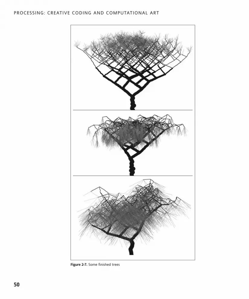
Figure 2-7. Some finished trees
PROCESSING: CREATIVE CODING AND COMPUTATIONAL ART
50
617xCH02.qxd 2/27/07 10:52 AM Page 50

Obviously, there are a lot of things I could still do with the tree code, but hopefully one ofyou will eventually take the code and improve upon it. I hope I was able to illustrate in thisexample how you can play with the code and even find stuff in the process of coding. Yes,there is some thinking involved, but there is also a lot of play and discovery. I’ve includedthe entire tree program following, with code comments for your hacking pleasure. If youwant to try running this, launch Processing and type (or paste) the code into theProcessing text editor.
/*algorithmic tree sketchIra greenberg, August, 2005*/
/* import Handy Java class withpublic x and y float props */
import java.awt.geom.Point2D;
// declare/define global variablesint counter;int counter2;float xg = 58;float yg = 46;int trunkSegments = int(random(7))+5;int nodeLimit = 20000;Point2D.Float[]pts = new Point2D.Float[nodeLimit];int branchLimit = 620;float trunkLength = int(random(50))+130;float[]lean2 = new float[trunkSegments+1];float radius = 26;
// initialize sketchvoid setup(){size(900, 600);background(255);stroke(30, 10, 5);
// create tree turnktrunk();
}
void trunk(){//draw trunkfor (int i=0; i<trunkSegments; i++){float lean = myRand(22);strokeWeight(radius+12);line(width/2+lean2[i], height-(trunkLength/trunkSegments)*i, !width/2+lean, height-(trunkLength/trunkSegments)*(i+1));
lean2[i+1] = lean;}
CREATIVE CODING
51
2
617xCH02.qxd 2/27/07 10:52 AM Page 51

// set inital branch point from top of trunkpts[0] = new Point2D.Float(width/2+lean2[trunkSegments], !height-trunkLength);
//create branchesbranch(pts);
}
//main function that draws branches and leavesvoid branch(Point2D.Float[]pts){int stemCount=2;
// global variable branchLimit controls complexity of treeif (counter2<branchLimit){
//set branch thicknessstrokeWeight(radius);
// some conditionals change branches as// they get further away from the trunkif(counter2<200){yg-=random(.354);xg-=random(.625);
if (radius>2) {radius*=.931;
}
} else if(counter2>=200){// at top of tree branches get thinner and more numerousstemCount = 2+(int)(Math.random()*15);// leave colorstroke(random(60), 50+random(90), random(20), 230);
yg-=myRand(.65);xg+=random(1.5);
radius*=(.91);}for (int j=0; j<stemCount; j++){// randomize branch positionsfloat xx= myRand(30);float yy= myRand(40);
/* commented out line below generates straight branchesline(pts[counter2].x, pts[counter2].y, pts[counter2].x+xg+xx,!pts[counter2].y-yg+yy);
*/
PROCESSING: CREATIVE CODING AND COMPUTATIONAL ART
52
617xCH02.qxd 2/27/07 10:52 AM Page 52

// generates organic looking branchesorgLine(pts[counter2].x, pts[counter2].y, !pts[counter2].x+xg+xx, pts[counter2].y-yg+yy);
/* fill up pts array to be passed back recursively to branch function */
pts[counter+1] = new Point2D.Float(pts[counter2].x+xg+xx, !pts[counter2].y-yg+yy);
// alternate branches left and rightxg*=-1;
// keep track of nodescounter++;
}
// keeps track of branchescounter2++;
//recursive callbranch(pts);}
}
// generates organic-looking branchesvoid orgLine (float x1, float y1, float x2, float y2){
int sections = 8;
float xd = x2-x1;float yd = y2-y1;
float twist;float[]twist2 = new float[sections+1];
for (int i =0; i<sections; i++){twist = myRand(5);line(x1+xd/sections*i+twist2[i], y1+yd/sections*i, !x1+xd/sections*(i+1)+twist, y1+yd/sections*(i+1));
twist2[i+1] = twist;}}
//generate a random val between (-n, n)float myRand(float val){return random(val)+random(-val);
}
CREATIVE CODING
53
2
617xCH02.qxd 2/27/07 10:52 AM Page 53

SummaryIn this chapter, I introduced creative coding as an approach to programming that inte-grates both analytical and creative processes. Using my friend Mark as an example, Idescribed some of the stereotypes and biases that can make this cross-brain integration sochallenging—a problem often (and sadly) reinforced in the classroom, which helped moti-vate me to teach creative coding and eventually write this book.
I gave a very top-view description about how Processing works, built on top of the Javaprogramming language, and I described some ways of structuring your code, includingprocedural and object-oriented approaches—both utilized within Processing. I tried todemystify the term “algorithm” and show the relationship between an algorithm and itsimplementation in code. I also discussed the challenge of learning to think like a “dumb”machine.
Finally, I covered the important role of happy accidents in the creative coding process, andI illustrated the point with an algorithmic tree example. In the next chapter, you’ll begin toexplore the actual nuts and bolts of coding.
PROCESSING: CREATIVE CODING AND COMPUTATIONAL ART
54
617xCH02.qxd 2/27/07 10:52 AM Page 54

617xCH02.qxd 2/27/07 10:52 AM Page 55

617xCH03.qxd 2/27/07 10:57 AM Page 56

3 CODE GRAMMAR 101
617xCH03.qxd 2/27/07 10:57 AM Page 57

This is where the techie stuff really begins! Hopefully, in the last two chapters you’ve got-ten some context and maybe even inspiration and are ready to dive right in. This chapterlooks at the nuts and bolts of programming in general. I make the assumption that youhave no experience with coding at all, so for those of you coming to Processing fromanother language, you may want to skim this chapter. In Chapter 4, I cover the basics ofgraphics coding, and in Chapter 5, I discuss the details of the Processing environment.
For new coders, my recommendation is to read this chapter at least once, but to not worryabout retaining all this info before continuing on. The material will sink in as you beginprogramming, and you can refer back to this chapter from time to time as a reference.Most of what I cover in this chapter is general programming theory and basic syntax andsemantics using Processing and to some degree Java. By syntax, I mean the way language isput together to form actual statements, functions, classes, and so on. Semantics refers tothe actual meaning of the code we write. Most of what I cover here, especially the theo-retical stuff, is applicable to other languages besides Processing, but of course each lan-guage has its own syntax, so the actual code will look different. Without further ado, Ipresent: Coding . . . really, really simplified.
Structure and abstractionThere are a couple of ways to think about structure in coding. On the simplest level, youcan think of structure in terms of the syntax you use to write a single line of code. Forexample, ball.x = width-ball.width;. On the other end of the spectrum, structure caninvolve applying complex rules and protocols for integrating large, convoluted softwaresystems. Fortunately for your needs, most of the structural issues will be pretty straight-forward. You will use basic syntactic structure to order a program, not unlike how youwould structure any written document, using punctuation, sentence structures, para-graphs, and so on. In coding, there are some other more abstract notions of structure thatI will discuss as well.
Our brains like some sense of order—although the range of chaotic tolerance among dif-ferent people’s brains seems pretty wide (as my office usually attests to). When a programgets overly complicated, it becomes hard to keep track of what’s going on. This oftenbecomes an especially vexing problem when you take a break from a project and thenpick it up some time later. There are a number of structures or abstractions commonlyused in coding to help order the process. The two major programming approaches I willcover are procedural programming and object-oriented programming (OOP). I introducedand defined both briefly in Chapter 2. Procedural programming relies on reusable blocksof code that work like processing machines, which you call when you need them. Thesereusable blocks of code are referred to as functions. The second approach, OOP, is a farmore ambitious and abstract approach that models a programming problem using con-cepts from the real world. For example, if you were writing an object-oriented program togenerate a virtual garden, you would create code structures, called classes, to organizeyour program. The classes might each describe a garden concept from the real world: leaf,vine, flower, sunlight, water, and so forth.
PROCESSING: CREATIVE CODING AND COMPUTATIONAL ART
58
617xCH03.qxd 2/27/07 10:57 AM Page 58

Your first programIn most programming books, the first program written is called “Hello World” (seeFigure 3-1). This spectacular program spits back the words “Hello World” to the screen—yawn! Needless to say, I find this program extremely boring and also think it sets the wrongtone for an entire book on creative coding. I for one need more encouragement and inspi-ration before attempting to learn something as scary and potentially boring as program-ming. Thus in breaking with tradition, which this book is all about, the first program youwrite will be entitled “Hello Earth.” Here it is:
/*Program Title: "Hello Earth"Program Description: Blue circle on black backgroundBy Ira Greenberg, August 5, 2005Comments: Our first Processing program- yippee!*/size(200, 200);background(0);// keep stroke from showing up around circlenoStroke();fill(80, 220, 255);ellipse(100, 100, 100, 100);print("Hello Earth!");
If you haven’t done so yet, download Processing from http://processing.org/download/index.html. I recommend selecting the standard download option. The installer willcreate a Processing directory. Within this directory, you’ll find the Processing applicationicon. Launch it, and type the “Hello Earth” sketch code into Processing’s text editor (thebig, white area in the middle of the application); then press the right-facing arrow in thecircle, at the top of the application.
Figure 3-1. Your first Hello Earth program
CODE GRAMMAR 101
59
3
617xCH03.qxd 2/27/07 10:57 AM Page 59

Congratulations! OK, so maybe it wasn’t a huge improvement to “Hello World,” but yougot to make a pretty, blue circle. Let’s look at the program line by line.
/* and */ are block comment tags, used to comment out multiple lines of information sothat it is ignored by the compiler. // can be used to comment out a single line. It is typicalat the top of a program to put some info about what your program does, who created it,the creation date, and any other special notes. This is not required, but most people putsomething up there. In fact, some people put a lot of stuff up there, including specificcode usage rights. How much you include up there doesn’t really matter because it won’taffect how your program functions. However, novellas, mission statements, and manifestosshould probably be put other places. Here are some more examples of comments:
// this is a valid comment
/* this is a valid comment */
/*this is a valid comment*/
// this// is also// a valid// comment
After the comments, I skipped a line. This is called whitespace. Whitespace in Processingand Java is disregarded, as it is in many other programming languages. You can put as muchwhitespace as you like to help you visually organize your code. The next line in the pro-gram, size(200, 200); is a function call (I spoke about functions in Chapter 2—functionsare reusable blocks of code that you call when you need them). You know this because ofthe parentheses after the word size. As stated in Chapter 2, a function call . . . well . . .calls a function—in this case, a function named size. The numbers within the parenthesesare called arguments—things that are passed to the function, which the function expectsto receive and makes use of. In this case, the numbers represent the width and height ofthe sketch window. When more than one argument is passed to a function, as insize(200, 200);, commas are used to separate the individual arguments. There is no limitto the number of arguments you can pass to a function, as long as the function has thesame number of parameters to receive the arguments. In addition, they must be sent tothe function in the same order that the function expects to receive them. In the case ofthe function calls in the Hello Earth example, the functions I called are all built into theProcessing language, and thus you can’t see the actual function definitions. I’ll bediscussing functions in much greater detail later on in this chapter. For now, let’s keepmoving.
At the end of the size(200, 200); call, you should notice a semicolon. Semicolons incoding are like periods in normal human language. They let the compiler know where theend of the statement is. A statement is simply a command to the program to do some-thing. In Processing, failure to include a semicolon results in a compiler error—an error
PROCESSING: CREATIVE CODING AND COMPUTATIONAL ART
60
617xCH03.qxd 2/27/07 10:57 AM Page 60

message comes up on the bar in the message area of the Processing editor window thatsays Expecting SEMI . . .. Fortunately, the Processing/Java compiler is smart and keeps youfrom making too big a goof-up. If you happened to try this, just put the semicolon back,and the program should compile fine. You’ll notice almost all the rest of the lines of theprogram have the same basic structure, each calling a function. As I mentioned previously,the line // keeps a stroke from showing up around the circle is a single-line comment.
The line noStroke(); is a function call that doesn’t pass any arguments. noStroke()affects how things are painted to the screen. The function call disables a stroke or outlinefrom being rendered on a shape. I’ll be covering Processing’s drawing and painting func-tions a lot in future chapters. The line print("Hello Earth!"); is a call to the print()function that expects an argument of type String. In this case, you passed in your "HelloEarth!" argument. You should have seen the words Hello Earth come up in the black textarea at the bottom of the Processing editor window. String is a type of data in Processing(or most any program) for referencing groups of characters. print() is an important func-tion that you’ll use all the time in Processing to help you debug your code. Processing hasan alternate version, println(), which does the same thing as print(), but adds a returnafter printing the string argument within the parentheses. For example, if you run the fol-lowing code:
print("hello");print("earth");
the output will be as follows:
helloearth
If you use the println() version, as follows:
println("hello");println("earth");
the output will look like this:
helloearth
The rest of the function calls in the program, Background(0), fill(80, 220, 255), andellipse(100, 100, 100, 100), set the background color, set the shape fill color, and cre-ate the circle, respectively. I will be covering these and other Processing graphics functionsin more depth beginning in Chapter 6.
Curly bracesAnother important and widely used syntactical structural element is the curly brace: { }.Curly braces, which always work in balanced pairs (an open and closed pair), are used tostructure blocks of code. Following are some code examples that show the use of curlybraces.
CODE GRAMMAR 101
61
3
617xCH03.qxd 2/27/07 10:57 AM Page 61

Here’s a conditional if...else example:
if (thisBook == bestSeller) {sleepWellAtNight();
} else {addMorePictures();
}
Here’s a function example:
void sleepWellAtNight() {println("one sheep, two sheep...");
}
Here’s a for loop example:
for (int i = 0; i < totalPictures; i++) {makeSomeInterestingPictures();
}
You’ll be looking at a lot more examples that make use of curly braces shortly. You’ll noticethat I structured the blocks of code between the curly braces using indentations. Indentingis not necessary for the code to work, but it is the conventional way to write blocks ofcode. Indenting makes it easier for other coders to read your code. In the examples in thisbook, each indentation is created by hitting the spacebar twice.
Dot syntaxThe last syntactical structure you’ll see in Processing is the dot (.) It looks like a period(and it technically is a period), but it’s referred to as a dot; it’s the same dot in .com. Thedot is an advanced syntactic structure used in OOP.
As I mentioned earlier, there are two approaches to structuring a program in Processing:procedural programming and OOP. Procedural programming uses functions to organize aprogram. You just saw an example of a function in sleepWellAtNight. When you need touse a function, you explicitly call it—for example, sleepWellAtNight()—pretty simple.
In OOP, you build much more complex structures called classes. To use a class, you createinstances of it, known as objects. Classes contain properties and methods. You can think ofthe properties as the traits of the object and the methods as actions you perform on/withthe traits. For example, if you create a class called Cat, some of the properties might becolor, weight, and markings, and a method might be getBreed(). You use the dot syntaxas a way to connect an object with its properties and/or methods. For example, if youcreate an object myCat from the Cat class, the object can call the getBreed() methodusing dot syntax, like this:
String breedName = myCat.getBreed();
PROCESSING: CREATIVE CODING AND COMPUTATIONAL ART
62
617xCH03.qxd 2/27/07 10:57 AM Page 62

Since the getBreed() method would return the name of a breed, you call the method aspart of an assignment statement so that the returned named will get assigned to the vari-able breedName. I’ll be covering OOP in much more detail in Chapter 8.
Naming conventionsPerhaps you noticed that a bunch of the fictitious names I used in the examples were com-binations of multiple words—for example, sleepWellAtNight() and getBreed(). This isreferred to as camelback notation. It is common to use it in case-sensitive environments.By capitalizing the initial character of the multiple words, you can read them more easily.Notice that the initial letter of the first word isn’t capitalized. Camelback notation is notrequired, but highly recommended. However, there are some required naming rules.
Legal names can only contain letters, underscores, numbers, and the dollar sign. The initialcharacter must be a letter, underscore, or dollar sign—not a number. I recommend onlyusing a letter as your initial character. Following the initial letter, it’s fine to use numbers.It’s also strongly suggested that you use names that are descriptive. For example, which iseasier to understand: getAge() or abdi()?
The names you define are called identifiers. Based on the preceding rules, here are somelegal identifiers:
String myBall
float speed
int ballCount
float theBallSpeed
boolean YouCanActuallyMakeYourVariableNamesAsLongAsYouLike
String BALL_MANUFACTURER
Here are some illegal ones. Can you tell why?
String Ball 1
int 100bjs
float -weight
int myBall#
The reasons are as follows: Ball 1 is illegal because of the space in the identifier; 100bjsis illegal because you can’t begin an identifier with a number; and -weight and myBall#are illegal because both use illegal characters: - and #, respectively.
CODE GRAMMAR 101
63
3
617xCH03.qxd 2/27/07 10:57 AM Page 63
LiteralsAs you will learn in the next section, a variable is something that can mean different thingsin different parts of the program. However, a literal is simply an explicit number or stringconstant (words or characters) used in programs. Here are some examples:
"Sophie"
25
10346
"abc"
Note that string literals are enclosed in quotes (usually double quotes) and numeric liter-als are not. In some cases, if you need a string within a string, you surround the inner stringwith single quotes. Here’s an example:
"One of Shakespeare's most famous lines 'to be or not to be' is in Hamlet"
Here’s a sketch that outputs some literal values:
String announceDate = "I'm writing this on: ";String currentMonth = "March ";int currentDay = 5;String currentDayName = "Sunday";int currentYear = 2006;String comma = ", ";
print(announceDate);println(currentDayName);print(currentMonth);print(currentDay);print(comma);println(currentYear);
This sketch will output the following:
I'm writing this on: SundayMarch 5, 2006
Notice how I used the print() and println() statements to help me format the out-putted lines combining the literals.
PROCESSING: CREATIVE CODING AND COMPUTATIONAL ART
64
617xCH03.qxd 2/27/07 10:57 AM Page 64

VariablesVariables are essential to programming, and it is hard to imagine coding anything withoutthem. In Processing and Java, there are two types of variables: primitive variables andobject reference variables. The major differences between these two categories of vari-ables are the kind of data they can be associated with and how this data is stored and ref-erenced in memory. I’m only going to cover primitive variables here; I’ll discuss objectreference variables when I cover OOP in Chapter 8.
A primitive variable is a simply a name assigned a specific value in memory that you canrecall and change. Here are a couple of examples of primitive variables:
int age = 6;String name = "Ian";boolean isABoy = true;
The first part of each of the statements (int, String, and boolean) declares what type ofprimitive data the variable can hold: int holds integers, String holds words, and booleanholds true or false. The next part (age, name, and isABoy) is the identifier of the variable,and the last part is the actual value (6, "Ian", and true) assigned to the variable.
Variable names in Processing and Java are case sensitive, meaning that xSpeed is a differ-ent variable than xspeed. A variable’s name is created by the coder and needs to be a legalidentifier, which was described previously. Regardless of whether you are naming a primi-tive variable, object reference variable, function, method, class, or object, the same legalidentifier–naming rules apply. There are also some reserved keywords that you shouldavoid using when naming things. The reserved keywords can be found here: http://java.sun.com/docs/books/tutorial/java/nutsandbolts/_keywords.html. In addition, Iwould also strongly recommend not naming your custom variables, functions, objects, andso forth with any of the built-in function names in Processing; it will lead to, at best, unex-pected results.
When I initially create a variable by writing int ballCount, I am not yet specifying a spe-cific value to be assigned to the variable, but only letting the computer know what type ofdata is allowed to be assigned to the variable (in this case, an integer). Every variable mustbe associated with a data type. Some common primitive data types in Processing are int,float, char, and boolean. Data types tell the variables what they can or can’t do, and alsohow much memory should be allocated for them. For example, a boolean type variablecan only hold the values true or false, requiring only 1 bit of memory to store either asingle 0 (false) or a 1 (true). It would be a waste of memory to store it any other way. Abyte can hold a number between –128 to 127 (that’s 256 different possible values), whichrequires 8 bits, or 1 byte, of memory.
CODE GRAMMAR 101
65
3
617xCH03.qxd 2/27/07 10:57 AM Page 65

When you write the variable data type and identifier (name)—for example, intballCount—you refer to this as declaring the variable. When you give a variable a specificvalue—for example, ballCount = 3—then you say you are initializing the variable. Thesetwo activities can be done together in one step (e.g., int ballCount = 3), or separately,depending upon your program needs. Because variables are by default mutable, once youinitialize a variable you can still change its value whenever you need to (as long asyou assign it a value consistent with its originally declared data type). For example, try run-ning the following code:
int ballCount = 15;println(ballCount);ballCount = 10;println(ballCount);ballCount = 100;println(ballCount);
When you run this sketch, you’ll get the following output:
1510100
Strict typingI remember first learning Java and being confused that I had to keep writing the data typesas I declared my variables, not to mention the whole case-sensitivity issue. I was used toold-school ActionScript, where variables could hold anything at any time. However, I’vecome to understand and appreciate the benefits of what’s referred to as “strict typing” ofvariables. Interestingly, ActionScript, which some of you may know, now uses explicit typ-ing of variables as well—so much for the good old days. So int ballCount can only holdinteger values and float ballSpeed can only hold float values. But why is this helpful?
You might be curious as to why you can get 256 unique values from a single byte (8bits) of memory. If you get scared by this explanation, don’t worry. It’s not essential toknow! It’s because in base 2 (as opposed to the base 10 system our minds are accus-tomed to), a byte is an 8-digit binary number, made up only of a combination of zerosand ones. The number of distinct values of a binary number can be calculated by tak-ing 2—only two possible values for each digit, 0 or 1—and raising it to the power ofthe number of places or digits in the number. So 2 to the 8th power equals 256. intscan hold up to 4 bytes (or 2 to the 32nd power), and thus can hold numbers between–2,147,483,648 and 2,147,483,647. If you’ve been involved in digital design for sometime, you’ve probably converted images from 24-bit color to 8-bit color, going from 2to the 24th power, or 16,777,216 possible colors, to 2 to the 8th power, or 256 possi-ble colors. The old web-safe palette of 216 colors was just a subset of the 8-bit palettethat looked somewhat consistent on different platforms/browsers.
PROCESSING: CREATIVE CODING AND COMPUTATIONAL ART
66
617xCH03.qxd 2/27/07 10:57 AM Page 66

It’s because strict typing helps create more precise and ultimately faster-running code. Ifyou try to assign a float value—for example, 3.2—to int ballCount, Processing will spitback a compiler error that says
The type of the right sub-expression, "float", is not assignable to the variable, of type "int".
This may seem obnoxious and a royal pain, especially if you are used to a loosely typedlanguage, but it really is a useful (or at least justifiable) language feature. Save for thestrange worlds of quantum physics, we would expect distinct whole balls to be held inballCount—not parts of balls. If the compiler let you assign 3.2 (maybe entered due to atypo) to ballCount, your program would probably crash later on. To debug your program,you would then have to track down a tiny but fatal type conversion error (definitely not ahappy coding accident). Additionally, in languages that do permit on-the-fly data typeassignment, it takes more work for the computer to figure out what type of data is held ina variable.
Because you set the data type of variables when they are declared in Processing and Java,and that information gets put in the compiled bytecode, the virtual machine (the languageinterpreter) needs to do less work. Languages like Processing and Java that work this wayare called statically typed languages. Languages like Python, on the other hand, aredynamically typed, and, due in part to dynamic typing, run slower than Java andProcessing. Now, at the risk of really getting you rankled, what do you think would happenif you tried to assign 3 (an integer) to ballSpeed (declared as type float)? Surprisingly,you wouldn’t get a compiler error. Huh! That seems to go against what I just wrote abouthow static typing works. The reason the compiler allows it is because the compiler con-verts the 3 to 3.0 automatically. Let’s test this out. If I try running the following code:
float ballSpeed;ballSpeed = 3;println(ballSpeed);
I get the following output:
3.0
The reason the compiler lets me get away with this is because there is no danger, nor anyreal change, to the value. 3, 3.0, and even 3.0000000000000 are all equal. Not to get toogeeky, but this type of implicit conversion is called a “widening conversion,” where an intis automatically converted into a float. The rule is that any primitive type will be con-verted implicitly (without any help from you) into any other type only if that type supportsa larger value; a float supports a larger value than an int. In regard to Processing, thatwould include byte to int and int to float. Bytes can become integers and integers canbecome floats. Converting the other way, from a float to an int to a byte (a “narrowingconversion”) can actually also happen, but you have to do it explicitly (which involves alittle work on your part), with something called type casting, which I’ll cover later in thebook. For now, let’s put this theory stuff to bed and play with variables a little.
Here’s a little program to create a stepped radial gradient (see Figure 3-2). Later on whenI cover loops, I’ll simplify this program, and also show you how to generate a more elegantcontinuous gradient. You’ll create the program in three stages. The first stage will fill the
CODE GRAMMAR 101
67
3
617xCH03.qxd 2/27/07 10:57 AM Page 67

display window background with black. The second stage will add a white ellipse, andthe third stage will create the gradient. In stages 2 and 3, you just need to add the newcode shown in bold. Also, try running the sketch at each stage to see the effect of addingthe new code.
Stage 1 just generates a black 200-by-200-pixel display window:
/*title: fun with variablesdescription: stepped radial gradientcreated: August 7, 2005by: Ira Greenberg*/
// set the sketch window size and backgroundsize(200,200);background(0);
Stage 2 utilizes some variables and draws a white ellipse in the middle of the display window:
/*title: fun with variablesdescription: stepped radial gradientcreated: August 7, 2005by: Ira Greenberg*/
// declare some global variablesint xpos;int ypos;int gradientWidth, gradientHeight;
// set the sketch window size and backgroundsize(200,200);background(0);
// radial width/heightgradientWidth = gradientHeight = width;
//radial center ptxpos = width/2;ypos = height/2;
//turn off stroke renderingnoStroke();
//create ellipsesellipse(xpos, ypos, gradientWidth, gradientHeight);
PROCESSING: CREATIVE CODING AND COMPUTATIONAL ART
68
617xCH03.qxd 2/27/07 10:57 AM Page 68

Stage 3 adds the gradient:
/*title: fun with variablesdescription: stepped radial gradientcreated: August 7, 2005by: Ira Greenberg*/
// declare some global variablesint xpos;int ypos;int interval;int gradientWidth, gradientHeight;
// set the sketch window size and backgroundsize(200,200);background(0);
// define variable values// controls banding of gradientinterval = 255/5;
// radial width/heightgradientWidth = gradientHeight = width;
//radial center ptxpos = width/2;ypos = height/2;
//turn off stroke renderingnoStroke();
//create ellipses//set fill color and render ellipsefill(interval);ellipse(xpos, ypos, gradientWidth, gradientHeight);fill(interval*2);ellipse(xpos, ypos, gradientWidth-interval, gradientHeight-interval);fill(interval*3);ellipse(xpos, ypos, gradientWidth-interval*2,!gradientHeight-interval*2);
fill(interval*4);ellipse(xpos, ypos, gradientWidth-interval*3,!gradientHeight-interval*3);
fill(interval*5);ellipse(xpos, ypos, gradientWidth-interval*4,!gradientHeight-interval*4);
CODE GRAMMAR 101
69
3
617xCH03.qxd 2/27/07 10:57 AM Page 69

Figure 3-2. Completed stepped radial gradient
I begin the program with my standard “about the program” comments. Then I declaresome global variables at the top of the program. Global, as opposed to local, means thatthe variables will be available from any place within the program. Later, when I cover func-tions, I’ll discuss this concept, called scope, further. You’ll notice I declared all the variablesas type int. The line int gradientWidth, gradientHeight; declares both gradientWidthand gradientHeight variables as type int in one line. When declaring and initializing vari-ables, you can put them on individual lines or bunch them together. For example, thefollowing line is perfectly legal:
int var1 = 3, var2 = 5, var3 = 6, var4 = 0;
I declare four variables of type int, while also initializing them with initial values.
After declaring variables, I set the size properties and background color of the sketchwindow:
size(200,200);background(0);
You might recognize these as function calls, in which dimensions (width and height) andcolor arguments are passed to the respective Processing functions. These functions arebuilt into the Processing language, which is why you don’t see the functions defined in theprogram anywhere. After you set the sketch window dimensions using the size(200, 200)command, you can then retrieve the sketch window size using Processing’s built-in globalproperties: width and height. You’ll notice these words turn a reddish color in the editorwhen you type them in, letting you know they are built-in properties in Processing.
PROCESSING: CREATIVE CODING AND COMPUTATIONAL ART
70
617xCH03.qxd 2/27/07 10:57 AM Page 70

Next, I assign values to some primitive variables:
// controls banding of gradientinterval = 255/5;
Because the gradient will go from black to white, I made the interval variable a factorof 255 (255 equals white). This way, I can step from black to white an equal number ofsteps—in this case, five. The next line may look a little strange:
// radial width and heightgradientWidth = gradientHeight = width;
If I write it out in English, its meaning will be clearer: the value of width is assigned to thevariable gradientHeight, which is then assigned to the variable gradientWidth. When youuse the single-equal sign (=), it means assignment, not equals. Assignment statements areevaluated right to left, which is why this compound assignment statement works. Also,remember that width is a built-in Processing property that holds the width I made thesketch window with the function call size(200, 200). gradientWidth and gradientHeightare variables I declared that will hold the width and height of the gradient. I could havewritten the statement in two lines, as well:
gradientHeight = width;gradientWidth = gradientHeight;
Setting the center of the gradient, I defined the variables xpos and ypos with the expres-sions width/2 and height/2, respectively. If you’ve never coded before, it may look odd touse a mathematical expression as something to be assigned, but it’s perfectly legal andcommon in programming. Remember, computers are really just super-powerful (andexpensive) calculators.
xpos = width/2;ypos = height/2;
The line noStroke(); turns off any stroke rendering, which is on by default in Processingwhen you render an ellipse or rectangle. noStroke() is another built-in Processing func-tion. The rest of the program paints the gradient:
fill(interval);ellipse(xpos, ypos, gradientWidth, gradientHeight);fill(interval*2);ellipse(xpos, ypos, gradientWidth-interval, gradientHeight-interval);fill(interval*3);ellipse(xpos, ypos, gradientWidth-interval*2, !gradientHeight-interval*2);
fill(interval*4);ellipse(xpos, ypos, gradientWidth-interval*3, !gradientHeight-interval*3);
fill(interval*5);ellipse(xpos, ypos, gradientWidth-interval*4, !gradientHeight-interval*4);
CODE GRAMMAR 101
71
3
617xCH03.qxd 2/27/07 10:57 AM Page 71

The fill(interval) lines are calls to Processing’s built-in fill() function. The calls passan argument to the function that controls the fill color of the shapes. In this case, I’mworking with grayscale values between 0 and 255. The ellipse(x, y, w, h) function callhas four arguments for the x and y position and width and height of the ellipse. You’ll alsonotice that the arguments I pass to the ellipse functions are both other variables andexpressions that include variables. Try running the program, if you haven’t already doneso, and changing some of the values and/or expressions to see what happens. See also ifyou can increase the number of steps in the gradient, making it a little smoother. When weget to loops, I’ll recode this for you, and you’ll really see the power of code for doingrepetitive tasks or iteration.
OperatorsSome of you may remember the word operator from math class. Operators are thesymbols you use when you write mathematical expressions. Technically speaking, opera-tors perform a function on operands. In the expression x + 3, x and 3 are the operands and+ is the operator. In terms of coding, you’ll primarily use the same four operators youlearned about in grade school: +, –, *, and /. Just using these operators, you’re able toperform almost all the math you need to create amazing visuals. Processing and Javahave additional operators besides these four, some of which I’ll go over as well. Beginningto use operators is pretty simple. Coding can get complex, however, when you’re figuringout the right combinations of operators needed in forming more complex expressions.You’ve already seen a bunch of operators in action in the last section on variables.For example, in the function call ellipse(xpos, ypos, gradientWidth-interval*4,gradientHeight-interval*4), the third and fourth arguments passed to the ellipsefunction, gradientWidth-interval*4 and gradientHeight-interval*4, each used twooperators (– and *). Because operators return a value, you are able to use them as argu-ments, as shown previously.
Here are some assignment operations utilizing the four basic operators. I’ll also go oversome basic rules that control the order in which operators do their thing, which is referredto as operator precedence.
int x = 4+3-6;float y = 14*3/5-2.34;float z = 14*3/(5-2.34);
The order of calculation is as follows:
Parentheses
Multiplication and division
Addition and subtraction
When operators have the same precedence level, the expression is evaluated from left toright.
PROCESSING: CREATIVE CODING AND COMPUTATIONAL ART
72
617xCH03.qxd 2/27/07 10:57 AM Page 72
In the first preceding example, addition and subtraction have the same precedence level,so the right side of the assignment statement is evaluated from left to right. (The assign-ment itself still occurs from right to left.)
The second example combines multiplication, division, and subtraction. Multiplication anddivision operations occur before subtraction. Since multiplication and division are at thesame precedence level, this expression is evaluated left to right.
The last example uses the same operands and operators as the second example, but usesparentheses to group. Since parentheses have the highest precedence, the subtraction inthe parentheses happens first, and then the multiplication/division occurs from left to right.
I’ve covered all the arithmetic operators but one: %, called the modulus operator. When Ifirst learned about this operator, I found it confusing and a little scary looking and sound-ing. It’s actually not such a big deal. The modulus operator doesn’t mean percent, butrather returns the remainder of the division between two operands. The remainder is thepart left over after the division.
For example, 7 % 2 would evaluate to 1, since 2 goes into 7 three times, leaving a remain-der of 1. Here are some more examples:
17 % 9 evaluates to 8.
6 % 3 evaluates to 0.
23.4567 % 5 evaluates to 3.4567.
In addition to the five arithmetic operators you just looked at, there are quite a few oth-ers. However, you only need to concern yourself with the most common ones for now.These operators can be broken down into three categories: the equality and relationaloperators, the conditional (also sometimes referred to as logical) operators, and theassignment operators.
Relational operatorsThe relational operators are very important, and you will use them often. Most of theseoperators should look familiar to you from grade school (although probably not the last two):
> (greater than)
>= (greater than or equal to)
< (less than)
<= (less than or equal to)
== (equal to)
!= (not equal to)
The greater than and less than arrows work the same way you remember them fromschool. They can also be used in conjunction with the = sign, which simply tests if oneoperand is greater/less than or equal to another operand. When you test with any of theseoperators, you’re testing whether the condition is true. For example, if(4<=5) orif(3>6)—the first test is true, since 4 is less than 5, and the second test is obviously false.
CODE GRAMMAR 101
73
3
617xCH03.qxd 2/27/07 10:57 AM Page 73

With regard to the last two operators (== and !=), the double-equal sign (==) tests forequality, and the symbols != test for inequality; therefore, in the following (non-code)lines:
if(3==3) would be true.
if(3!=3) would be false.
if(3!=5) would be true.
Conditional operatorsThe relational operators are often used in conjunction with two conditional operators forcreating somewhat more complex conditions to evaluate. The two operators are
&& (logical and)
|| (logical or)
One minor warning: The operator terms relational and conditional (and also logical) areused inconsistently, especially around the Web. I’m classifying the operators as specifiedon Sun’s site. See http://java.sun.com/docs/books/tutorial/java/nutsandbolts/opsummary.html for more info.
Following are some examples. To check if x is greater than 3 and less than 10:
if (x > 3 && x < 10) {//code in here would only //execute when condition is true
}
To check if x is less than 20 or greater than 50:
if (x < 20 || x > 50) {//code in here would only execute //when condition is true
}
To check if the boolean variable myLecturesAreBoring is not true:
if (!myLecturesAreBoring) { //code in here would only execute when //condition is true-which is always!!
}
By putting the exclamation symbol in front of myLecturesAreBoring, you are actuallychecking for the value to be false.
The relational and conditional operators are used to control the logical flow of your pro-gram. In addition to using the keyword if, you can combine it with the keyword else.These types of statements, which control the branching logic in your programs, are calledconditional statements. I’ll discuss them in more detail a bit later in this chapter.
PROCESSING: CREATIVE CODING AND COMPUTATIONAL ART
74
617xCH03.qxd 2/27/07 10:57 AM Page 74

Assignment operatorsThe only other operators you need to look at for now are used for assignment operations.
The simplest assignment operation just uses the = operator. For example, to assign thevalue 55 to the int variable speed, you’d simply write the following:
int speed = 55;
Again, the = sign is used for assignment, not equality. When you test for equality inProcessing and Java, instead of writing if(speed=55), you need to write if(speed==55).The first way actually assigns the value 55 to speed; the second way tests if speed is actu-ally equal to 55. Using the single-equal sign when testing for equality is a very commonmistake new coders make. We’ve been conditioned to think of equality as =, not ==, so itmakes sense that new coders find it confusing.
When I write an assignment statement, for example
x = 4;
I am assigning 4 to x. So now the value of x evaluates to 4. Let’s say I want to add 3 to x—I could write x + 3, right? Let’s try it.
Write the following two lines of code in Processing and click run.
int x = 4;x + 3;
Surprised you got an assignment error? It’s because you’re adding 3 to x, but not assigningthe solution anywhere. Remember that computers are really dumb. If they can’t put thevalue anywhere, they don’t know what to do. Fortunately, the Processing compiler sendsout a compiler error letting you know this.
You can fix the preceding assignment in a couple of ways—but the easiest way to add 3 tox, and then assign the value back to x, is as follows:
x = x + 3;
Now this may look a little odd, having something assigned to itself. But reading the expres-sion in English helps: add the value of x and 3 and then assign that value to x. Assignmentoperations happen from right to left. It may take a little time playing with this to get itclear in your brain. These operations work the same way for the other mathematical oper-ators as well. Here’s a division example:
float y = 10.4;// divide by 1.25y = y / 1.25;
CODE GRAMMAR 101
75
3
617xCH03.qxd 2/27/07 10:57 AM Page 75

These operations are so common in programming that there is a shortcut syntax morecommonly used. The shortcut simply joins the mathematical and assignment operators.For example, the last expression (y = y / 1.25;) could be shortened to the following:
y /= 1.25;
The other mathematical operations follow the same structure. Here are some examples:
float temp = 98.6;temp += 5; // temp now equals: 103.6temp -= .6; // temp now equals: 103temp *= 2; // temp now equals: 206temp %= 23; // temp now equals: 22
The last expression may look odd; it’s using the modulus operator. Remember, modulusreturns the remainder of division; 23 goes into 206 eight times, leaving a remainder of 22,which then gets assigned back to the temp variable.
In the assignment operations you’ve been looking at thus far, the operator(s) have beensurrounded by two operands. The geeky way to refer to these types of operators is asbinary operators. Processing also uses some operators that only require one operand,which are referred to as unary operators. Two of these very useful operators are actuallyshortcuts for two other shortcuts.
If I want to add 1 to the int variable x using the shortcuts just shown, I could write thefollowing:
x += 1;
Using a unary operator, the expression can be shortened to the following:
x++;
You’ll also see this expression written as ++x;. It does matter, in some contexts, on whichside you put the two operators, which I’ll discuss the subtlety of later on. Besides incre-menting by one, you can also decrement by one, using x-- (also --x). I recommend learn-ing to use the shortcuts as soon as you can—they will save you keystrokes (possibly stavingoff carpal tunnel) and make you look like you’ve been coding for years.
ConditionalsNext, I want to cover conditional statements, which you got a sneak peak of when youlooked at the relational and conditional operators. A conditional statement is sometimesreferred to as a decision statement. Essentially, is says that if a certain condition is true,then do something; but if it is not true, do something else.
I think by now you’re probably in need of some visual digression, so we’ll cover the condi-tionals by creating a little sketch (see Figure 3-3), which creates a bouncing ball:
PROCESSING: CREATIVE CODING AND COMPUTATIONAL ART
76
617xCH03.qxd 2/27/07 10:57 AM Page 76

/*title: Bouncing Balldescription: ball deflects off sketch window edgescreated: August 9, 2005by: Ira Greenberg*/
// declare global variablesint xspeed, yspeed;int xpos, ypos, wdth, ht;
//initialize sketchvoid setup(){
//set sketch window size and background colorsize(400, 400);background(0);
//ball speedxspeed = 3;yspeed = 6;
//ball sizewdth = 10;ht = 10;
// turn off shape stroke renderingnoStroke();
//initial ball placementxpos = width/2;ypos = height/2;
frameRate(30);}
// begin animation loopvoid draw(){
//update backgroundbackground(0);
//draw ballellipse(xpos, ypos, wdth, ht);
//upgrade position valuesxpos+=xspeed;ypos+=yspeed;
CODE GRAMMAR 101
77
3
617xCH03.qxd 2/27/07 10:57 AM Page 77

/*conditionalsdetects ball collission with sketch window edgesalso accounts for thickness of ball*/if (xpos>=width-wdth/2 || xpos<=wdth/2){xspeed*=-1;
}if (ypos>=height-ht/2 || ypos<=ht/2){yspeed*=-1;
}}
Figure 3-3. Screen capture of the Bouncing Ball program
When you run the Bouncing Ball program, you should see a little white ball moving in thesketch window and deflecting off the window edges. The code may look a little scary atfirst glance, but most of it has been covered (at least in theory). I suggest taking a littletime and messing around with some of the values and seeing what happens. The worstthing you’ll do is break the program. When you’re done getting a little well-deserved playout of your system, you can read the brief discussion of the program that follows. Don’tworry if this sketch seems over your head. I don’t expect most readers to be able to fullygrasp it yet. I’ll be going over sketches like this many times in future chapters. My maingoal here is just to give you something interesting to look at and play with.
As usual, I start the program with some comments and then declare global variables. Thesetup(){ ... } function is built into Processing and is used to initialize the program anddefine variables that may be needed later on; it runs just once. The draw() { ... } func-tion is also built into Processing and is used for animation. When you have a single CPU inyour computer, it can only really do one thing at a time. However, it can execute processesso fast that, to our slow brains, it seems like many things are happening simultaneously.
PROCESSING: CREATIVE CODING AND COMPUTATIONAL ART
78
617xCH03.qxd 2/27/07 10:57 AM Page 78

Animation is a perfect example of this effect. If at least 12 images per second move infront of your eyes, you begin to see continuous movement. But of course, you are reallyonly looking at a series of static images.
The frameRate(30) function call at the bottom of the setup() function controls the rateat which the animation runs. You can pass different values to the frameRate() call as asingle argument between the parentheses to change the speed of the animation. If youdon’t include the frameRate() call, the default speed is 60 frames per second. I suggesttrying some different values in the call to see how it affects the speed and smoothness ofyour animation. The draw() function below setup() controls animation in Processing.Simply by including it, an animation loop is created in your sketch, which I’ll cover in a lotmore detail later.
In the draw() function, I update the background color, which helps create the illusion ofthe bouncing ball. Try commenting out the background(0) line by putting two forwardslashes (//) in front of the command, and watch what happens. The effect is actuallypretty cool, and what you would do if you wanted the background to be incrementallypainted, rather than entirely updated each loop iteration.
Next I call the ellipse function, ellipse(xpos, ypos, wdth, ht);, passing in the four vari-ables for the ball’s x position, y position, width, and height. Then I increment the xpos andypos variables using the assignment shortcut operators. This gets the ball moving.However, the ball will never stop, so I need to do some thinking for the computer and setup some conditions for when the ball should deflect or bounce off the frame.
The two conditional statements are essentially identical, except of course one controls thex movement and the other the y movement. So what I describe following for x also appliesto y.
I begin the conditional with if. if is a reserved word in Java and Processing that expects acondition to follow it surrounded by parentheses. Conditional statements rely on Booleanlogic (true or false) to decide how to respond. The default test is for truth. So when I writeif(someStatement == true), I could also just write if (someStatement), which automat-ically checks for truth. If the conditional statement is true, program execution occurs onthe next line following the test statement. For example:
if (5>4)print("hello");
The program should output hello. Although you can write your statement the way I didpreviously without curly braces, when there is only one line of code after the if statement,I don’t recommend it. Instead, I recommend always writing it like this:
if (5>4) {print("hello");
}
The curly braces make it easier to read your conditional statements, and as you begin towrite more complex statements, you’ll need the curly braces anyway. If you do not use thecurly braces, then only the next line of code will be executed if the condition is true.
CODE GRAMMAR 101
79
3
617xCH03.qxd 2/27/07 10:57 AM Page 79

Again, I always use the curly braces and will throughout the book. Getting back to the con-ditional statement in the bouncing ball sketch, I am actually checking for either of twoconditions at the same time:
if (xpos>=width-wdth/2 || xpos<=wdth/2){xspeed*=-1;
}
This may look a little scary. Sorry, I had to choose between four separate conditional state-ments or two scary looking ones. In actuality, it’s not too bad. The two vertical lines in themiddle of the parentheses (||) are used to write “or” in Processing/Java. The way “and” iswritten is &&. So the test statement is checking to see if either statement is true. If eitheris true, then the ball is hitting the right edge or the left edge of the frame window, and thecode between the curly braces executes.
What’s important to remember in this sketch is that the event loop is continuously run-ning; that means all the code within the draw() block is running around 30 times per sec-ond, so the test is running continuously as the ball moves. If the conditional test were upin the setup() function, it would only run once, and the window edge detection wouldn’toccur. When the ball’s position (really the xpos value) is greater than or equal to the widthof the frame minus half the width of the ball (or xpos is less than or equal to half the widthof the ball), the xspeed variable is turned positive or negative, depending on what its cur-rent state is. Remember from grade school math that when you multiply a positive and anegative number you get a negative, but two negatives multiplied equals a positive. Sincexpos keeps adding the value of xspeed to itself, if the speed is positive, the ball moves tothe right, and if it is negative, it moves to the left—creating the illusion of it beingdeflected off either of the frame wall edges. Everything I just described works the sameway for the conditional statement to check the ball’s y position.
I realize that this still may be confusing. I suggest playing with the code a little, settingsome more extreme values to see what happens. I will be covering animation in a lot moredetail later in the book, so this information will be revisited. For now, I want you to grasphow and why to use conditional statements.
Sometimes when you are checking for a condition, you want to offer one execution pathif you find a condition to be true, and another one if you don’t. For example:
if (hunger>=starving){eatAnything();
} else {eatWhatIsHealthy();
}
The if statement will execute the lines between the first pair of curly braces ({ eatAnthing(); }) if the condition between the parentheses (hunger>=starving) is true.If the condition is false, the code following the else statement will execute ({ eatWhatIsHealthy(); }). The conditional statement has two paths. You’ll soon realizethat there are a number of ways in coding to do the same thing. Some uptight computerscientists might tell you that there is a most efficient way to write code, but I don’t totallybuy that. Efficiency is a good thing, but you also need to find a style that suits your per-sonality. For example, I could rewrite the preceding statements as follows:
PROCESSING: CREATIVE CODING AND COMPUTATIONAL ART
80
617xCH03.qxd 2/27/07 10:57 AM Page 80

if (hunger<starving){eatWhatIsHealthy();
} else {eatAnything();
}
The code works the same way—although it could maybe execute a little faster if mostpeople are not starving. However, it is also more difficult to think about something notbeing equal vs. something being equal. Do what feels right to you, and don’t obsess aboutefficiency or writing perfect code; it doesn’t exist.
The last conditional example sent you down two possible pathways, depending onwhether something was true or not. However, there are ways of checking among multiplepossibilities by using a series of if...else if statements. For example:
if (hunger >= starving) {eatAnything();
} else if (hunger <= starving && belly < full) {eatWhatIsHealthy();
} else if (hunger <= starving && belly==full) {eatDessert();
} else {stopEating();
}
When the code is run, each conditional statement will be checked until a condition is true,at which time the code between the curly braces following the true conditional statementwill execute. For example, if my hunger is less than starving and my belly is full, the codeeatDessert() will execute. If none of the of the conditional tests are true, the codefollowing else ({ stopEating(); }) will execute. The final else statement, which is notrequired, will always execute when none of the proceeding if...else if statements eval-uate to true.
One word of caution: When you begin getting your coding legs and cranking out all kindsof conditional tests, pay close attention to the logic in your statements. If you make a logicerror, your sketch may run without any compiler error, but you may not get the results youwanted. Logic errors are sometimes tricky to track down, because the compiler doesn’thelp you. Using println() statements and checking the values of your variables is nor-mally the way to track down a logic bug.
switch statementWhen you find yourself writing long if...else if statements, you may want to thinkabout using a switch (sometimes also referred to as a case) statement. switch statementsare just like if...else if statements, except that each conditional test usually has a built-in exit strategy. Here’s an example switch statement:
CODE GRAMMAR 101
81
3
617xCH03.qxd 2/27/07 10:57 AM Page 81

switch (numberOfBurritosEaten){case 0:orderSuperBurrito(2);break;
case 1:orderSuperBurrito(1);break;
case 2:orderGrandeBurrito(1);break;
case 3:orderRegularBurrito(1);break;
case 4:orderTacos(2);break;
case 5:orderTacos(1);break;
case 6:orderDessert();break;
default:seekHelp();break;
}
switch statements, unlike if...else if statements, can’t check a range, but rather checkfor a specific value match. The condition inside the parentheses after the word switchneeds to be of type int, char, or byte. The int type is for integers (e.g., –5, 0, or 2300),the char type is for individual characters on the keyboard (e.g., i, a, or /), and the bytetype is a subset of integers—values between 127 and –128. I tend to use int valuesbetween the parentheses of my switch statements to keep things simple. In the newestversion of Java (1.5), as of this writing, you can also use what’s called an enumerated typewithin the parentheses of switch statements (not currently in Processing). However,enumerated types are an advanced concept that I’m not going to cover here.
When the switch statement runs, the value in the top parentheses is compared to eachcase, from top to bottom. If there is a match, the code after the colon is executed until itcomes across a break. When it finds a break statement, the program exits the switch state-ment and goes to the next line below the entire switch block. The break command isoptional, but if you don’t use it, the program will fall through and execute the code of thenext case, and continue checking all the remaining cases until it reaches the bottom of thestatement. In most instances, this would be a waste of processing power. The defaultstatement (also optional) at the end of the switch executes if no case matches were found.The last break statement is unnecessary and harmless, but possibly helpful if you happento add more statements below and convert it to a case, so you don’t eventually forget toadd the break statement (a common error). I leave the choice to you.
PROCESSING: CREATIVE CODING AND COMPUTATIONAL ART
82
617xCH03.qxd 2/27/07 10:57 AM Page 82

Ternary operatorThe last conditional structure I want to show you is Java’s ternary operator—meaning thatit uses three operands. The ternary operator takes some time getting used to, and somepeople never get used to it. I tend to hardly ever use it, but other people use it a lot, so it’sworth learning. It’s logic is similar to an if...else statement. Here’s an example:
//some variablesint karma;boolean isStillReadingThisBook;
// Here's the if/else version:if (isStillReadingThisBook){karma = 100;
else {karma = 50;
}// Here's the ternary operator version:karma = isStillReadingThisBook ? 100 : 50;
The ternary version looks pretty terse and cryptic. Its form is really a throwback to an olderstyle of programming. However, as you can see, it is efficient. The condition is tested, inthis case the boolean variable isStillReadingThisBook; if the condition is true, then thefirst value after the ? is returned and assigned to the karma variable; if it is false, thenthe value after the : is returned. It’s really up to you whether you want to use this struc-ture. You can always use the more verbose if...else to accomplish the same thing.
Arrays and loopsThe next section looks at arrays and loops. I’ve grouped these somewhat large topicstogether because of their interconnectedness. Arrays and loops aren’t that complicated asconcepts, but they can get a little hairy for newbie coders to implement. I’ll be using themto expand on two previous sketches: the stepped radial gradient and the bouncing ball.These examples will illustrate the power of arrays and loops and also begin to show youthe potential of code as a creative medium.
ArraysThere are times in coding when you’ll want to assign many values to a single variable. Forexample, maybe you have 100 balls and you want to keep track of each of their x posi-tions. The problem with using a primitive variable is that it can only hold one value at atime. Thus, you would need 100 separate variables to account for each ball’s x position.Arrays were developed to solve this problem; they are single data structures that holdmultiple values. If I wanted to animate all 100 balls, there are very easy ways to change the100 x positions stored within the array. You can think of an array as a desk with multipledrawers. On the one hand, an array is a single entity, referred to by a single name; on theother hand, the array can hold many separate values, each accessible through an indexing
CODE GRAMMAR 101
83
3
617xCH03.qxd 2/27/07 10:57 AM Page 83

system, which I’ll discuss shortly. Arrays are a little difficult to get your head around at first,but they are absolutely critical to coding, and you’ll be using them lots throughout thebook. So if some of this explanation feels a bit abstract, don’t worry—you’ll be revisitingthese concepts again and again.
Arrays don’t have a default data type, but rather are declared with a data type just likevariables are. Following is an example of an array declaration:
int[] xpos;
The declaration is done the way you’d declare a regular int variable, with the addition ofthe two brackets. Here are two more array declarations:
float[] xspeed;String[] names;
You see the pattern—the type comes first, then the brackets and then the identifier orname of the array. You’ll notice in the two declaration lines that I wrote “float” in all low-ercase, but “String” with an initial cap. This was not an arbitrary decision on my part; floatis a primitive data type and needs to be all lowercase. String is the name of a class, andthe convention is to name a class with an initial cap. I’ll be covering classes later in thebook, but for now you can think of a class as representing a unique data type—which youcan use when you declare a variable, or in this case an array.
Arrays can be any size (actually as large as the int data type, which is big enough) andhold any legal type. However, once they are declared, their type cannot change, and oncethey are initialized, their size cannot change. Therefore, if I declare
float[] xspeed;
then the xspeed array can now only hold values of type float (real numbers). Here’s howto initialize the xspeed array:
xspeed = new float[100];
The keyword new reserves space in memory for the array. You‘ll be using the keyword newa lot more when we get to OOP.
Now the xspeed array has 100 places in memory reserved for float values. Its size, like itsdata type, is now immutable, meaning that it can’t be changed. The array now has space inthe computer’s memory reserved for it, although it still doesn’t have any specific valuesassigned to those 100 places. The two lines can be put together into one declaration andinitialization statement:
float[] xspeed = new float[100];
Here are a few more examples of declaring and initializing arrays:
int[] items = new int[50];String[] itemNames = new String[10000];Object[] obs = new Object[0];
PROCESSING: CREATIVE CODING AND COMPUTATIONAL ART
84
617xCH03.qxd 2/27/07 10:57 AM Page 84

The items array has 50 places reserved in memory for ints. The itemNames array has10,000 places reserved in memory for Strings, and the obs array has 0 spaces in memoryfor Objects. In general, you wouldn’t initialize an array with 0 items, but you could. Finally,there is one additional way to initialize an array, when you know ahead of time what willbe in it:
int[] speeds = {2, 4, 445, -120, 3, 90, 54};
This array will have a length of 7, and, like all arrays, its size can’t be changed. Here’sanother example with a String array:
String[] names = {"Lulu", "Ivan", "Myrna", "Pookie"};
So, once you declare and initialize arrays, how do you use them? An index system is usedto access the values (called elements) stored at the different positions in the array. It’s avery simple system with one caveat: arrays are zero-indexed, which means the first posi-tion in the array is at position 0, not 1. There are some benefits to this, which you’ll seeshortly when we get to for loops, but in the beginning it can be confusing.
Going back to the previous array, int[]speeds = {2, 4, 445, -120, 3, 90, 54}, toaccess the first item—the value 2—I use speeds[0]; to access the third item, 445, I usespeeds[2]; and for the last item, 54, I use speeds[6]. Make sure you understand thisbefore you move on; it’s important. Arrays also have a built-in length property that you’lluse often. You access the property with dot syntax. To find the length of the speeds array,you write speeds.length.
The length of the array is the actual number of items in the array, so speeds.length isequal to 7, even though speeds[6] gives you the last item in the array. You should see howworking with arrays is both simple and a little complicated.
Finally, if you try to access an index that is out of range—for example, if you try to accessspeeds[7], which doesn’t exist—you’ll get a compiler error. This may seem like a pain, butagain it’s there to help you.
LoopsOne of the best uses for computers is handling repetitive, redundant tasks that are tootedious for most people. This is accomplished in programming by using structures calledloops. Loops are structures that continue to run, or execute, until some condition is metthat causes them to stop. The two types of loops listed in the Processing language refer-ence are while loops and for loops. In addition, we’ll look at one other variation on thewhile loop called a do...while loop.
whileHere’s an example of a while loop, (which I don’t recommend you run):
while (true) {println ("help I'm in an infinite loop");
}
CODE GRAMMAR 101
85
3
617xCH03.qxd 2/27/07 10:57 AM Page 85

while is a reserved keyword in Processing, like the keywords if and else, which you’vealready looked at. A while loop will execute the code between its open and closed curlybraces as long as the condition between the parentheses is true. In the example, the con-dition will always be true. true is actually another reserved keyword in Processing and Javathat always means, well . . . true. Can you see why I didn’t want you to run this loop exam-ple? It will never stop running, as there is no exit condition (i.e., a condition that whenreached will cause the code to continue past the loop). Nasty loops like this are calledinfinite loops, and they are to be avoided. Of course, you can force the Processing appli-cation to quit, so don’t panic if you did try running it (against my sage advice). Here’s animproved and safe version of that last demonic loop:
int x = 0;while (x<100) {println (x);x += 1;
}
If you run this, you should see the numbers 0 through 99 printed in the text output areaat the bottom of the Processing application. The while loop runs as long as x is less than100. With each cycle of the loop, the value of x is incremented by 1. Here’s one moreexample:
int x = 1000;while (x>=0) {println (x);x -= 100;
}
This loop outputs the values 1000 through 0, decrementing by 100 each cycle, or iteration,of the loop. Also, I set the condition using >=, so 0 was output as well.
do . . . whileA while loop will only execute if the condition is true. However, there are times whenyou’ll want a loop to execute at least once no matter what. The do...while loop is sort ofa backward while loop that always executes at least once, regardless of whether the con-dition is true. After the first iteration of the loop, though, it behaves just like a regularwhile loop. Here are two examples:
//example 1.int x = 50;do {println(x);x += 1;
}while(x<50);
//example 2.int x = 40;do {
PROCESSING: CREATIVE CODING AND COMPUTATIONAL ART
86
617xCH03.qxd 2/27/07 10:57 AM Page 86

println(x);x += 1;
}while(x<50);
In the first example, the condition is false. Yet if you run this code, you’ll get a single out-put of 50, because the loop will always execute at least once. In the second example, thecondition begins true, and you get an output from 40 to 49, just as you’d expect using astandard while loop.
forThe for loop is my favorite loop (if that doesn’t sound too pathetic). It does basically thesame thing as a while loop, but I find the process of using it more elegant, especially inregard to dealing with arrays, which is where this whole discussion is going. Here’s a forloop example:
for (int i=0; i<50; i++){println(i);
}
The for loop looks a little odd at first. There are three individual areas within the paren-theses, in the head of the for loop:
int i=0; (initialization)
i<50; (condition)
i++ (counter)
In the example, I created the variable i of type int and initialized it to 0. The next part ofthe loop checks to see if i is less than 50, and the third section increments i by one. Thesemicolons terminate each of these distinct sections in the for loop head, just like a nor-mal end of line. Notice, however, that there is no semicolon after the counter. If youhaven’t yet, try running the example.
You should see output from 0 to 49. Even though the loop incrementation is at the headof the for loop, the variable i is not incremented until after the code in the block is exe-cuted. That’s why the first value is 0, not 1.
One of the real benefits of the for loop is that the variable (i), which is declared in the ini-tialization part of the loop, is sort of a secret variable that can only be seen between thecurly braces of the for loop. This secret status is referred to as local scope. Local scopemeans that the variable is only known within the structure it is defined within. Local scopeallows you to use another variable named i somewhere else in the same program or evenin another separate for loop, without having the two names conflict or create ambiguityin the program. It is very common practice, and a coding convention, to use the letters i, j,and k as the names of local variables used as counters in loops. Normally, when I write aprogram that includes a number of simple for loops, I’ll name each of the counter vari-ables i. Besides local scope, you can also declare variables with global scope. When youdeclare variables outside of any structures (normally at the top of your program), these
CODE GRAMMAR 101
87
3
617xCH03.qxd 2/27/07 10:57 AM Page 87

variables have global scope, meaning that they can be seen from anywhere within yourprogram, including within loops. In the earlier while loop example, the variable x hasglobal scope and can be seen anywhere in the program:
int x = 1000;while (x>=0) {println (x);x -= 100;
}
Thus, you would not want to use x again as a counter in another loop later in the sameprogram, as it could cause unpredictable results. Because the for loop solves this problemby keeping the counter variable local in scope, I tend to use for loops far more often thanwhile loops.
In the next section, “Functions,” I’ll go more into detail on local vs. global scope. Here area couple of other examples of for loops:
for (int i=1000; i>50; i-=2)println(i);
}
for (int i=1000, j=200; i>50; i-=2, j++)print("i = ");println(i);print("j = ");println(j);
}
The top example is just a variation on the for loop discussed previously. It just countsdown by two instead of counting up by one. The second loop example uses multiple vari-ables and incrementors in the head—which is legal. You just separate the differentvariables with commas. Try running this last loop example to view the output; it will helpyou understand how the for loop runs.
for loops can add tons of efficiency to your code, and used cleverly can really cut downon the number of code lines. As an example, I’ve recoded the stepped radial gradient (seeFigure 3-4) using a for loop, converting it into a smoother continuous gradient.
//Continuous radial gradientsize(200,200);background(0);
for (int i=255; i>0; i--){noStroke();fill(255-i);ellipse(width/2, height/2, i, i);
}
PROCESSING: CREATIVE CODING AND COMPUTATIONAL ART
88
617xCH03.qxd 2/27/07 10:57 AM Page 88

Figure 3-4. Continuous radial gradient
If you don’t remember, the original stepped gradient example was about four times aslong and not nearly as pretty.
Finally, in the latest version of Java (1.5), as of this writing, there is a new variation on thefor loop, called a for-each loop, or enhanced for loop. I am not going to cover it, as it isnot currently supported in Processing. Information about it can be found on Sun’s site athttp://java.sun.com/j2se/1.5.0/docs/guide/language/foreach.html.
Processing efficiencyYou already saw that arrays hold multiple values and loops allow you to repeatedly exe-cute code. You can use these two structures together to form a powerful and highly effi-cient data processing system. As an example, here’s a simple mail merge program thatoutputs mailing addresses in the text area of the Processing application. The data is storedin six separate arrays, for first names, last names, street, city, state, and country.
// mail merge program//create some arrays with address dataString[]firstName = {"Ira ", "Sophie ", "Ian ", "Robin "}; String[]lastName = {"Jed", "Rose", "Isaac", "McLennan"};String[]street = {"4 Happy Ln, ", "19 Hunan Pl, ", !"104 Hevi Hevi St, ", "1000 Donkey Dr, "};
String[]city = {"Oxford", "Changsha", "Easton", "Edinboro"}; String[]state = {"Ohio, ", "Hunan, ", "Pennsylvania, ", "Scotland, "};String[]country = {"USA", "China", "USA", "UK"};
// use a for loop to generate mergefor (int i=0; i<firstName.length; i++){print(firstName[i]);println(lastName[i]);
CODE GRAMMAR 101
89
3
617xCH03.qxd 2/27/07 10:57 AM Page 89

print(street[i]);println(city[i]);print(state[i]);println(country[i]);println();
}
The sketch outputs the following:
Ira Jed4 Happy Ln, OxfordOhio, USA
Sophie Rose19 Hunan Pl, ChangshaHunan, China
Ian Isaac104 Hevi Hevi St, EastonPennsylvania, USA
Robin McLennan1000 Donkey Dr, EdinboroScotland, UK
The for loop does all the heavy lifting by moving through the arrays, using the counter asthe index to the position in the arrays. Also notice in this example that I alternatedbetween print() and println() to format the address and line spacing correctly. Using afor loop to process four elements in each array may not seem too impressive. But imag-ine if each of the arrays included 10,000 elements. This simple sketch would have just aseasily processed and output all that address data as well (of course, it would have taken afew more seconds). To better illustrate this, let’s look at a more visually interesting exam-ple. I’m going to take the previous bouncing ball animation and beef it up some, usingarrays and a loop or two. I’ll also be incorporating one of Processing’s handiest functions:random(value), which generates a random value between 0 and the value argument.
This example is a little long—try not to panic. You’ll be looking at a lot of code like thisthroughout the book. I recommend running the sketch before reading through the code.You may even want to mess around with some of the values to see how it changes theoutput.
Here’s the Many Bouncing Balls program (see Figure 3-5):
/*title: Many Bouncing Ballsdescription: balls deflect off sketch window edgescreated: August 9, 2005by: Ira Greenberg*/// global variables
PROCESSING: CREATIVE CODING AND COMPUTATIONAL ART
90
617xCH03.qxd 2/27/07 10:57 AM Page 90

int ballCount = 500;int ballSize = 8;int ballSpeed = 3;float[]xspeed = new float[ballCount];float[]yspeed= new float[ballCount];float[]xpos = new float[ballCount];float[]ypos = new float[ballCount];float[]wdth = new float[ballCount];float[]ht = new float[ballCount];
//initialize sketchvoid setup(){//set sketch window size and background colorsize(400, 400);background(0);
//initialize values for all ballsfor (int i=0; i<ballCount; i++)
// set varied ball speedxspeed[i] = random(1, ballSpeed);yspeed[i] = random(-ballSpeed, ballSpeed);
// ball varied ball sizeswdth[i]= random(1, ballSize);ht[i]= wdth[i];
// set initial ball placementxpos[i] = width/2+random(-width/3, width/3);ypos[i] = height/2+random(-height/3, height/3);
}
// turn off shape stroke renderingnoStroke();//set the animation loop speedframeRate(30);
}
// begin animation loopvoid draw(){
/*updates backgroundcomment out to use alternatefill option below*/background(0);
for (int i=0; i<ballCount; i++){
CODE GRAMMAR 101
91
3
617xCH03.qxd 2/27/07 10:57 AM Page 91

/*To use this fill option:1. uncomment fill call below2. comment out the background function call above*/// fill(i*255/ballCount);
//draw ballsellipse(xpos[i], ypos[i], wdth[i], ht[i]);
//upgrade position valuesxpos[i]+=xspeed[i];ypos[i]+=yspeed[i];
/*conditionals:detects ball collision with sketch window edgesaccounting for ball thickness.*/if (xpos[i]+wdth[i]/2>=width || xpos[i]<=wdth[i]/2){xspeed[i]*=-1;
}if (ypos[i]+ht[i]/2>=height || ypos[i]<=ht[i]/2){yspeed[i]*=-1;
}}
}
Figure 3-5. Screen capture of the Many Bouncing Balls program
PROCESSING: CREATIVE CODING AND COMPUTATIONAL ART
92
617xCH03.qxd 2/27/07 10:57 AM Page 92
Hopefully, you were able to successfully run this sketch. I created an alternative renderingoption as well, which you can mess with in a bit. When you run the sketch, you should seemany (actually 500) white balls moving randomly around, bouncing off the edges of thewindow. This code is not simple, so don’t feel bad if it is a struggle to understand it. You’regoing to be doing a lot more of this type of coding beginning in Chapter 6—so this is reallymore like a teaser than something you need to fully grasp at this point. I just thought itwas good to show you something a little more interesting after all the hard work you’vebeen putting in. The main concept I want to reinforce at this point is the power of arraysand loops. Let’s look at the program in sections:
// global variablesint ballCount = 500;int ballSize = 8;int ballSpeed = 3;float[]xspeed = new float[ballCount];float[]yspeed= new float[ballCount];float[]xpos = new float[ballCount];float[]ypos = new float[ballCount];float[]wdth = new float[ballCount];float[]ht = new float[ballCount];
After my comments, I declare and initialize some global variables; these variables will beaccessible throughout the entire program. I chose the specific data type, in this case int orfloat, based on the type of value that would need to be stored in the respectivevariables/arrays. Obviously, ballCount could be an integer value, but a speed value wouldneed to be a float value. The arrays are initialized with enough memory to hold the totalnumber of balls. Remember, I can’t change the arrays’ sizes once they’re initialized (intruth, you’ll see later that there are indeed functions to do such a thing), so it’s importantto make them big enough at the beginning. Although the arrays are initialized to each hold500 values (based on ballCount), there is still nothing in them.
//initialize sketchvoid setup(){//set sketch window size and background colorsize(400, 400);background(0);
//initialize values for all ballsfor (int i=0; i<ballCount; i++)
// set varied ball speedxspeed[i] = random(1, ballSpeed);yspeed[i] = random(-ballSpeed, ballSpeed);
// ball varied ball sizeswdth[i]= random(1, ballSize);ht[i]= wdth[i];
CODE GRAMMAR 101
93
3
617xCH03.qxd 2/27/07 10:57 AM Page 93

// set initial ball placementxpos[i] = width/2+random(-width/3, width/3);ypos[i] = height/2+random(-height/3, height/3);
}
// turn off shape stroke renderingnoStroke();//set the animation loop speedframeRate(30);
}
After declaring the global variables, I do some program initialization in the setup() func-tion. I set the window size and background color, and then I use a somewhat hairy-lookingfor loop. In reality, it’s not that different from the single-ball setup() function, but arrayscan look intimidating until you get used to them. The for loop
for (int i=0; i<ballCount; i++)
uses the counter i, which is conveniently used as the first index slot in the arrays. I use theglobal ballCount variable as the loop limit (in this case 500), and I increment the loop byone each cycle. Thus, each iteration of the for loop will allow me to assign a value to eachposition in the arrays; it’s a very efficient system that works similarly to the mail mergeexample.
In the speed arrays, I’m getting a little fancy and adding some random numbers. As I men-tioned previously, I used Processing’s random() function, which can take either one or twoarguments. In the book’s appendix, I go through the Processing API and cover this functionin more detail. Basically, one argument generates a random number from 0 to the argu-ment value. Two arguments give you a random value between the range of the two argu-ments. Processing’s random() function returns a float value (a real number).
I initialized the arrays for the balls’ sizes and original positions in a similar fashion to thespeed arrays, utilizing some more random values. Last, I turned off the pesky stroke ren-dering (noStroke();) and set the frame rate to 30 for smooth animation. Whew . . . almostdone.
// begin animation loopvoid draw(){
/*updates backgroundcomment out to use alternate fill option below*/background(0);
for (int i=0; i<ballCount; i++){
/*To use this fill option:1. uncomment fill call below2. comment out the background
PROCESSING: CREATIVE CODING AND COMPUTATIONAL ART
94
617xCH03.qxd 2/27/07 10:57 AM Page 94

function call above*/// fill(i*255/ballCount);
//draw ballsellipse(xpos[i], ypos[i], wdth[i], ht[i]);
//upgrade position valuesxpos[i]+=xspeed[i];ypos[i]+=yspeed[i];
/*conditionals:detects ball collision with sketch window edgesaccounting for ball thickness.*/if (xpos[i]+wdth[i]/2>=width || xpos[i]<=wdth[i]/2){xspeed[i]*=-1;
}if (ypos[i]+ht[i]/2>=height || ypos[i]<=ht[i]/2){yspeed[i]*=-1;
}}
}
The draw() function is where all the magic happens. Once the draw() function is added tothe sketch, an event loop begins refreshing the screen approximately the number of timesper second specified with the frameRate(30) argument. The first thing I did was refreshthe background so that the balls don’t leave a trail through the window. I set an alternativerendering approach that utilizes this effect. If you read through the draw structure, I’ve putinstructions on how to get the trails to occur. But don’t do it yet—let’s finish the analysisfirst.
Next is the second for loop. This loop draws the ellipses, increments their respective x andy position values by the speed values, and performs collision detection—which in this casemeans that it checks if the ball’s x and y positions go beyond the window boundaries; ifthey do, that specific speed value’s sign within the array is reversed (positive to negative ornegative to positive). If xspeed is positive, then the ball moves to the right; if it’s negative,then it moves to the left. If yspeed is positive, then the ball moves down; if it’s negative,then it moves up.
Since all the data is housed in parallel arrays with the same number of indices, I am able toincrementally deal will all this stuff on each iteration of the for loop; this is the real powerof using arrays in conjunction with loops. Now I recommend you go back and try the alter-native rendering style (see Figure 3-6) and also mess with some of the values in the pro-gram. If you get something really cool, please e-mail me a screenshot. Finally, let me stressthat this stuff is complicated—especially to new coders. I don’t necessarily expect you toget all this yet. But hopefully some of it is beginning to stick. Many of the examples andtutorials throughout the rest of the book deal with similar patterns of coding, so I have nodoubt that if you stay the course, this stuff will gel.
CODE GRAMMAR 101
95
3
617xCH03.qxd 2/27/07 10:57 AM Page 95

Figure 3-6. Screen capture of an alternative rendering of the Many Bouncing Balls program
FunctionsI mentioned functions briefly in Chapter 2, so let’s look at them again in a little moredetail. Functions add structure and flexibility to your sketches, but also a little complexity.Try not to worry if some of the material seems too abstract—you’ll be using functionsthroughout the rest of the book. My main goal here is to give you an overview of basicprogramming structures and a glimpse into the potential of creative coding.
In the simplest sense, functions just organize code into reusable blocks. They also have theability to receive arguments and return a value. Here are some examples.
This first sketch draws a rectangle based on the x, y, width, and height properties passed tothe drawRectangle() function:
void setup(){size(400, 400);background(255);drawRectangle(150, 150, 100, 100);
}void drawRectangle(float x, float y, float w, float h){rect(x, y, w, h);
}
PROCESSING: CREATIVE CODING AND COMPUTATIONAL ART
96
617xCH03.qxd 2/27/07 10:58 AM Page 96

If you run this, you should see a 100-by-100-pixel square in the middle of the displaywindow.
When you write your own function, you need to include Processing’s setup() function, oryou’ll get a compile error when you try to run the sketch. A function begins with a returntype (either void or a legal data type); an identifier (the name of the function); open andclosed parentheses, with any optional declared parameters; and open and closed curlybraces.
Here’s the structure of a function:
return type (void or legal datatype) function name(optional !parameters){code to execute when function is called;
}
The drawRectangle(float x, float y, float w, float h) function in the precedingsketch expects four arguments to be passed to it when it’s called, as I specified fourparameters between its parentheses. You’ll notice that I use both the terms parameter andargument. This can be confusing to new coders (and even some experienced coders); Iprefer to call the values between the parentheses in the function definition parameters,and the values passed to the function arguments. I know this may sound like an issue ofsemantics (or worse), but I find it easier to discuss and teach this stuff by using the two dif-ferent terms.
This last example didn’t do much more than Processing’s plain old rect() call. The nextexample (see Figure 3-7) makes better use of the drawRectangle() function and alsorevisits for loops—yippee!
void setup(){size(400, 400);background(255);for (int i=0; i<100; i++)drawRectangle(random(width), random(height), random(200), !random(200));
}}
void drawRectangle(float x, float y, float w, float h){rect(x, y, w, h);
}
CODE GRAMMAR 101
97
3
617xCH03.qxd 2/27/07 10:58 AM Page 97

Figure 3-7. Random rectangles
This example begins to reveal the power of functions. By passing, or inputting, differentvalues to the function, you can generate very different results. Functions create efficien-cies by helping you avoid writing redundant code. They also free you from having to writeall your code linearly, from top bottom, in your sketch. Once you define a function, youcan call it when you need it, as well as multiple times, as I did in the last example. The nextsketch uses Processing’s built-in draw() function to move a box across the screen.Processing’s draw() function is called automatically when you include it in your sketch.The draw() function increments the value of two speed variables I created (xspeed andyspeed), which are assigned to two position variables I created (xpos and ypos). xpos andypos control the x and y positions of the box.
// simple ballint xpos, ypos;int xspeed=3;int yspeed=5;
void setup(){size(400, 400);
}
void draw(){background(0);rect(xpos, ypos, 10, 10); xpos+=xspeed;ypos+=yspeed;if (xpos>=width-10 || xpos<=0){xspeed*=-1;
}if (ypos>=width-10 || ypos<=0){
PROCESSING: CREATIVE CODING AND COMPUTATIONAL ART
98
617xCH03.qxd 2/27/07 10:58 AM Page 98

yspeed*=-1;}
}
Within the draw() function of this last sketch, I include very simple collision detection,used to reverse the direction of the box if it collides with any of the edges of the displaywindow. Imagine if there were a lot more detection code—it could get pretty confusinglooking. A better way to organize this would be to write a separate block of code (a func-tion) to check the collisions. Not only will this code be cleaner looking, but the detectionwill be in a sense encapsulated (a word I’ll discuss more when I get to OOP). Modularizingthe code like this in a function gives the ability to potentially plug the function into otherprograms. Also, once I develop a template for this collision detection, I can develop varia-tions on it, building a cool detection library—but I’m getting a bit carried way. Here’s thesketch with the collision detection function added:
int xpos, ypos;int xspeed=3;int yspeed=5;void setup(){size(400, 400);
}void draw(){background(0);rect(xpos, ypos, 10, 10);xpos+=xspeed;ypos+=yspeed;checkCollisions(xpos, ypos);
}
void checkCollisions(int xp, int yp){if (xp>=width-10 || xp<=0){xspeed*=-1;
}if (yp>=width-10 || yp<=0){yspeed*=-1;
}}
This new, improved code should execute exactly the same as the first version. Let’s gothrough the function line by line.
checkCollisions(xpos, ypos); probably looks familiar to you by now. It’s a functioncall—similar in form to size(400, 400). I pass two arguments (xpos and ypos) to thefunction. Also, since the function is not being assigned to some other variable, nor beingused in the place of a variable, you can assume a value is not being returned by the func-tion. If the function does not return any value, you use the reserved keyword void whenyou declare it; void takes the place of a data type that would need to be declared if thefunction did return a value. The function itself is almost exactly the same as the code thatwas inside the draw structure in the original version:
CODE GRAMMAR 101
99
3
617xCH03.qxd 2/27/07 10:58 AM Page 99

void checkCollisions(int xp, int yp){if (xp>=width-10 || xp<=0){xspeed*=-1;
}if (yp>=width-10 || yp<=0){yspeed*=-1;
}}
You’ll remember that a function head needs to have a data type or void; a legal identifier(name); and balanced (open/closed) parentheses, with any required parameters, includingtheir data types, between the parentheses. The parameters, declared between the paren-theses, in a sense catch the arguments passed to the function, and they need to match up.If the argument count or the data type doesn’t match what’s in the function head, thecompiler will let you know. You can also use multiple versions or variations on the samenamed function in your program, as long as the parameter lists are different—meaning adifferent number of parameters or different data types. For example, the following threefunctions could all be included in the same program without any ambiguity:
void myFunction(int x, int y){}void myFunction(int x, int y, int z){}void myFunction(float x, float y, float z){}
Since the first function uses only two parameters and the second and third functions usedifferent data types for the parameters (int and float, respectively), the compiler will seethese as unique functions. To call the functions, I could the use the following lines:
myFunction(2, 5);myFunction(2, 5, 7);myFunction(2.0, 4.2, 1.23);
If this looks strange to some of you who have experience with another language, thisworks in Processing because of an object-oriented feature built into Java called methodoverloading, which I’ll discuss when I get to OOP in Chapter 8. Next, let’s look at anotherfunction that returns a value to our current sketch. Here’s the new sketch code:
int xpos, ypos;int xspeed=3;int yspeed=5;void setup(){size(400, 400);
}void draw(){background(0);rect(getXMotion(), ypos, 10, 10); ypos+=yspeed;checkCollisions(xpos, ypos);
}
PROCESSING: CREATIVE CODING AND COMPUTATIONAL ART
100
617xCH03.qxd 2/27/07 10:58 AM Page 100

void checkCollisions(int xp, int yp){if (xp>=width-10 || xp<=0){xspeed*=-1;
}if (yp>=width-10 || yp<=0){yspeed*=-1;
}}
int getXMotion(){xpos+=xspeed;return xpos;}
void checkCollisions(float yp, float yp2){if (yp<=0){xspeed*=-1;
}if (yp<=0){yspeed*=-1;
}}
I changed the first argument in the rect() function call, rect(getXMotion(), ypos, 10,10), from a variable to another function call—which is legal, as long as the functionreturns a value. If you try to pass a function call as an argument that doesn’t return avalue, the compiler will give an error. The new function is declared with a return type ofint, instead of void, and the last line is a return statement.
int getXMotion(){xpos+=xspeed;return xpos;
}
You must have a return statement as the last line in any function with a return type otherthan void. If you don’t, you guessed it, the compiler will spit at you. There are times whenyou will use additional return statements in a function—for instance, when you haveif...else statements—but you still must have a return statement as your last line.
I want to make one more improvement to the sketch. The getXMotion() function handlesthe x position only, but what about the y position? Well, I’m sure you can see that I couldjust easily copy the getXMotion() function and convert it to a getYMotion() function.However, that seems like too much work, and the behavior of the two functions is identi-cal. When you find yourself repeating things or making fine adjustments to similar struc-tures, you should be thinking that there’s got to be a better way. In this case, there is. I canreturn an array of ints instead of a single int and convert the getXMotion() function to agetXYMotion() function. Here’s the new function:
CODE GRAMMAR 101
101
3
617xCH03.qxd 2/27/07 10:58 AM Page 101

int[] getXYMotion(){xpos+=xspeed;ypos+=yspeed;int[]xypos = new int[]{xpos, ypos};return xypos;
}
The function return type is now an int[] array, not a primitive int. The function createsan xypos array each time it’s called, and then returns the array. The other important aspectto this approach is knowing how to receive the array that’s passed back. When I was orig-inally just returning an int back, it was simple, because it was the only value returned. Butto really benefit from this approach, the rect() call needs to be changed from:
rect(getXMotion(), ypos, 10, 10);
to
rect(getXYMotion()[0], getXYMotion()[1], 10, 10);
Does this make sense? I know it looks pretty strange. Remember, arrays are indexed,beginning at [0]. When the array is passed back, it’s being received as a multivalue struc-ture, with xpos at the 0 index and ypos at the 1 index. These values are retrieved usinggetXYMotion()[0] and getXYMotion()[1], respectively. If this is still not making sense,imagine replacing getXYMotion() with the array. To get the value in the first position ofthe array, you’d use arrayname[0]. To get the value in the second position, you’d usearrayname[1]. I hope that helps. You’ll be doing stuff like this in future chapters, so try notto freak out if this stuff is hurting your head—it’s supposed to in the beginning.
The last thing I want to say about functions relates to a nasty habit many coders get into.Now don’t get any wrong ideas here. I’m talking about the use of magic numbers—whatwere you thinking of? Magic numbers are values we hard-code into a program that makethe program difficult to change or customize. Using magic numbers is generally not theway to develop a modular system, but it can be a fast way of hacking out a solution with-out thinking of the big picture. In general, you’ll want to avoid them. Following are twosimple examples—the first using magic numbers:
//sketch using magic numbers:size(200, 200);background(255);strokeWeight(5);stroke(20);fill(100);rect (50, 50, 100, 100);
The second example improves upon this sketch, using a parameterized function instead ofthe hard-coded values:
// sketch using a nice parameterized functionvoid setup(){size(200, 200);background(255);
PROCESSING: CREATIVE CODING AND COMPUTATIONAL ART
102
617xCH03.qxd 2/27/07 10:58 AM Page 102

createRect(50, 50, 100, 100, 20, 5, 100);}
// parameterized functionvoid createRect(int xpos, int ypos, int wdth, int ht, int strokeCol,int strokeWt, int fillCol) {stroke(strokeCol);strokeWeight(strokeWt);fill(fillCol);rect (xpos, ypos, wdth, ht);
}
Both sketches should output the same centered rectangle, as shown in Figure 3-8.
Figure 3-8. Rectangle generated initially using magic numbers and then with a function
Do you see how the second approach will allow you to create any rectangle, while the firstonly creates one? The more modular and general you can make your code, the greater thechance you can reuse it or easily expand it. However, this type of approach takes moreplanning and analysis, and sometimes you just want to get coding. Because this book isabout creative coding, I think it is perfectly acceptable to sometimes hack out poorlystructured, “ugly” code, especially if it allows you to express yourself and find new solu-tions more effectively. I suspect if you’re like me, you’ll eventually discover things that youwant to build out into larger projects, and that’s where the rules and best practices stuffbecomes important. So basically you have permission from me to write nasty code whennecessary (to remain creatively engaged), but don’t rat me out to your teacher or bosswhen they give you a hard time about it.
CODE GRAMMAR 101
103
3
617xCH03.qxd 2/27/07 10:58 AM Page 103

SummaryThat ends the procedural programming boot camp part of the book. I hope you’re not toobleary-eyed or despondent. This information takes time to assimilate, and again I suggestyou treat this chapter as a reference or cheat sheet to return to as you need it. Everythingcovered in this chapter will resurface in examples to come throughout the book, so you’llhave lots of opportunities for practice. Later, in Chapter 8, I’ll cover OOP, which will beyour “code boot camp part 2” experience. But of course by then, you’ll be a grizzled andseasoned codehead. The next chapter will look at some of the fundamental issues involvedin graphics programming.
PROCESSING: CREATIVE CODING AND COMPUTATIONAL ART
104
617xCH03.qxd 2/27/07 10:58 AM Page 104

617xCH03.qxd 2/27/07 10:58 AM Page 105

617xCH04.qxd 2/27/07 11:01 AM Page 106

4 COMPUTER GRAPHICS, THE FUN,EASY WAY
617xCH04.qxd 2/27/07 11:01 AM Page 107

This chapter gives a simplified and highly abridged overview of computer graphics.Graphics and visualization is one of the major research areas in computer science and hasa reputation for being highly complex and mathematically demanding. However, there is awide range of research being conducted under the heading “graphics and visualization”—with varying degrees of complexity. Dr. Edward Angel, in his widely read textbookInteractive Computer Graphics, lists four major application areas within computer graphics:
Display of information
Design
Simulation and animation
User interfaces
Display of information involves data visualization, which can range in complexity frombasic charting or plotting of simple data sets (e.g., business graphics), to visualizing molec-ular interactions or biological processes, to real-time mapping of complex dynamicsystems (e.g., modeling of the weather).
Design (really, computer-aided design) is applied in manufacturing, engineering, and archi-tecture. It integrates the visual (form) requirements with the analytical or structural (func-tion) requirements. For example, an architect can design a part of a structure visually,through the manipulation of planes and cubes and other simple geometry, while the sys-tem calculates underlying structural issues.
Simulation and animation is similar to display of information, but involves time—often realtime—and verisimilitude, or the appearance of reality. For example, a pilot can practiceemergency landings more safely in a flight simulator than in a real plane. Haptics, anotherrelated research area in computer science, involves tactility, or touch, that complementsvisual and aural (sound) data used in simulation to create an immersive, real-feeling virtualexperience.
User interfaces, sometimes referred to as GUIs (graphical user interfaces), make up thearea of computer graphics research that people are most familiar with. We are surroundedby interfaces—not just on our PCs, but on our watches, phones, cameras, appliances, auto-mobiles, and so forth. Yet, for all its ubiquity and apparent simplicity, user interfaceresearch is complex, because it deals with human interaction. An entire area of computerscience research is devoted to this important and challenging area, called HCI (human-computer interaction).
Processing is being used, to varying degrees, in all four of these areas, and as additionalcode libraries are developed by readers like you, Processing’s application in graphics andvisualization research and development will continue to expand. Unlike proprietary lan-guages like ActionScript and Lingo, built primarily around a specific market-driven appli-cation area (e.g., web development, CD-ROM/Kiosk development), Processing’s Java coreand open source status give it a vast breadth of application possibilities.
PROCESSING: CREATIVE CODING AND COMPUTATIONAL ART
108
617xCH04.qxd 2/27/07 11:01 AM Page 108

Some of the reasons coding graphics gets a reputation for being difficult is the mathinvolved in dealing with 3D space and the low-level algorithms needed to manipulate mil-lions of pixels in real time. 3D math is somewhat complicated, especially if you don’t havea basic grounding in linear algebra and trigonometry, neither of which are really that com-plicated, but are usually purged from most artist’s brains by the time they leave highschool (if it ever got in there in the first place). Because computer monitors are 2D sur-faces, there is a need in 3D to always convert 3D geometry back to a 2D projection, so wecan see it on the screen.
Computationally, graphics requires a fair amount of low-level processing and lots of mem-ory storage. For example, on a monitor with 1920 ! 1200 resolution, over 2,300,000 pixelsare redrawn about 70 times per second. Each pixel is made up of three color components(RGB), giving each of the 2 million–plus pixels a range of 16.7 million different colors.Once you add the actual calculations needed to generate 2D or 3D geometry, virtual lightsources, textures, special effects, animation, virtual cameras, and event processing (userinteraction)—well, you develop a lot of respect for engineers! As computers have gottenfaster and memory has gotten cheaper, graphics programming has benefited greatly andthings have gotten a little simpler, but less is definitely not more when it comes to graph-ics, and in spite of the technological advances, users continuously demand more fromtheir games, films, software, and personal devices. In this chapter, I am only going to dealwith 2D graphics and some basic math. In spite of all the complexity I just mentioned,Processing makes it pretty easy to get started with graphics (and of course I’ll continue totake things slowly). Although this chapter only deals with 2D, everything I cover is applica-ble to 3D, which I’ll cover near the end of the book.
Coordinate systemsA coordinate system is simply a numbered grid that allows you to locate a point in space.Two French mathematicians, René Descartes (1596–1650) and Pierre de Fermat (1601–1665)get credited with developing the Cartesian coordinate system; although Descartes getsmost, if not all, of the credit. The Cartesian coordinate system is really just an extension ofa number line. The number line has a 0 position; values to the right of 0 are positive andvalues to the left of 0 are negative—pretty basic stuff. In the coordinate system most of usremember from math class, there is a horizontal axis, usually referred to as x and a verticalaxis, referred to as y. The vertical axis has its own number line, and where these two per-pendicular number lines intersect (0, 0) is the origin. In the coordinate system we use inmath, above the y-origin is positive and below the y-origin is negative. In computer graph-ics, this is often flipped, as it is in Processing—above the y-origin is negative and below they-origin is positive. Figure 4-1 illustrates the coordinate system in Processing, in relation tothe monitor. You’ll notice that the origin is at the top-left corner of the coordinate system.
COMPUTER GRAPHICS, THE FUN, EASY WAY
109
4
617xCH04.qxd 2/27/07 11:01 AM Page 109

Figure 4-1. In Processing, the x-axis increases from left to right and the y-axis increases from top to bottom. The origin is in the top-left corner, at (0, 0).
If you draw a 40 pixel by 40 pixel rectangle on the monitor at (100, 100), it will be 100 pix-els to the right of the left edge of the monitor and 100 pixels down from the top edge ofthe monitor. Since you can only plot a point to a specific pixel location on the screen, youalso need to consider which point on the rectangle gets placed at (100, 100). This point issometimes referred to as the registration point. In most instances, the registration point iseither the top-left corner of the image or the center of the image. In Processing, there is afunction named rectMode() that allows you to specify from what point a rectangle isdrawn by passing different arguments to the function. For example, rectMode(CENTER)orients the rectangle at its center point, while rectMode(CORNER) uses the rectangle’s top-left corner; there is also a third argument, rectMode(CORNERS), which draws the rectangleby specifying two points: the top-left and bottom-right corners of the rectangle. In Figure4-2, the rectangle on the left is drawn from its top-left corner at (100, 100), and the oneto the right is drawn from its center point.
Figure 4-2. The square on the left uses its top-left corner for registration, while the one onthe right uses its center point. You can explicitly set the registration point using Processing’srectMode(MODE) command.
PROCESSING: CREATIVE CODING AND COMPUTATIONAL ART
110
617xCH04.qxd 2/27/07 11:01 AM Page 110

When working in a 3D coordinate system, you just add another axis, called z, which followsthe same rules I’ve been discussing for 2D. The z-axis goes into the screen and is perpen-dicular to both the x- and y-axes—but rest assured, for now you only need to deal with thex- and y-axes.
One other issue to consider when dealing with coordinate systems is local vs. world coor-dinates. For example, when you draw a rectangle on the screen at (100, 100), you can thinkof the rectangle living on the screen world at pixel address (100, 100). However, let’s imag-ine you then want to put a small circle on the rectangle 3 pixels to the right of the rectan-gle’s left edge and 3 pixels down from its top edge. What is the circle’s screen pixeladdress? You can consider the circle’s world address as (103, 103), and the circle’s localaddress, in relation to the rectangle, as (3, 3). Now this may sound a little confusing andlike an obscure point, but it is something that comes up fairly often. For example, it isoften easier to work with a local coordinate system when you are assembling componentson a larger structure. If you are drawing windows on a house, isn’t it easier to just worryabout where the windows fit in relation to the rectangle of the of building, rather thankeeping track of where the windows are in relation to the edges of the screen? This way, ifyou ever move the building, the windows will stay in the right place in relationship to thebuilding.
Anatomy of an imageA computer screen is (very simply put) a matrix, or grid, made up of rows and columns ofpixels that can each glow a certain color, giving the illusion, when enough pixels are glow-ing the right color, of a continuous tone image (e.g., a photograph). Fortunately, the reso-lution of most of our monitors is high enough and the refresh rate fast enough to allowthis matrix of pixels and constant screen redrawing to remain hidden, giving the illusion ofimage persistence—you see what looks like a still, smooth image. When you zoom wayinto an image in a program like Photoshop, you can see the pixel matrix, made up of littleblocks of color. If you look under a magnifying glass at printed materials, you can also seea matrix of dots of color that, when zoomed back out, creates the same illusion of a con-tinuous image as on a monitor. Some well-known artists, such as Roy Lichtenstein andChuck Close, both exploited this phenomenon in their paintings, albeit in very differentways. Lichtenstein painted the dot pattern as an explicit visual element in his pop art work,directly referencing the commercial printing process. Close utilized a matrix structure orig-inally as a production tool, dividing his images up, similar to a monitor, into small rectan-gular cells. Eventually his work began incorporating the grid as an explicit element as well.
Refresh rate is the rate at which the monitor redraws the screen image. Although imageson a screen look constant, they’re not. If you’ve ever shot video of your television, you’veprobably seen the screen flickering or jumping. The frequency of the video camera’srefresh rate and the frequency of the monitor’s refresh rate are not synchronized, allow-ing you to catch the screen refreshing. Properties like screen resolution and refresh ratesare hardware-dependent and determined by the monitor and video card in your com-puter. You can usually select from numerous monitor display configurations through sys-tem control panels to change these properties, but actually communicating directly withthe video card or monitor through the code you write in Processing is lower level than yougo. Java does have a DisplayMode class, allowing you the ability to mess with this stuff
COMPUTER GRAPHICS, THE FUN, EASY WAY
111
4
617xCH04.qxd 2/27/07 11:01 AM Page 111

(if you really want to). Above the hardware level is where you’ll do most of your graphicscoding in Processing.
No matter how high level the process of drawing to the screen is made for you, eitherthrough a programming language like Processing, or even more simply, a pencil tool in agraphics application, the same underlying stuff still needs to happen. These underlyingprocesses can be quite complex in a language like Java, and involve low-level processing,pretty close to the hardware. For example, there’s a class in Java called BufferedImage thatprovides access to much of the procedural and structural anatomy of an image. Happily,you don’t need to understand the BufferedImage class to work with images in Processing;but it can be helpful, or at least interesting, to see a little of what goes into creating animage behind the scenes. I really want to stress that you don’t need to understand any-thing about the BufferedImage class to work in Processing, but learning a little about itwill give you more insight into how images work in Java and in computer graphics in gen-eral. The BufferedImage class is composed of a bunch of other classes. Figure 4-3 shows asimplified diagram of its structure.
Figure 4-3. Simplified BufferedImage class structure
The BufferedImage class diagram looks pretty scary. I’ve had advanced computer sciencestudents brought to their knees trying to unravel it. What makes it so complicated is theabstraction involved in its design and ultimately the processing required to generate andmanipulate images on a computer screen. If you begin to feel sick to your stomach read-ing about this stuff, just skip ahead to the “Graphic formats” section.
fill(0, 0, 255);rect(0, 0, 10, 10);
These two lines of processing code draw a blue rectangle with a black stroke (border) tothe screen. Let’s look a little below the surface at what’s happening. The rect() functionin Processing, which relates to the Rectangle() method call in Java, is a drawing methodbuilt into the Processing language. You simply pass four arguments to the rect() function:x, y, width, and height, and the function draws a rectangle to those specifications. Drawingmethods usually work by plotting points, called vertices (singular is vertex), and then con-necting the vertices with some type of line. In Processing, as in numerous other program-ming languages with graphics capabilities, there are drawing methods to draw points, lines,and basic shapes (simple polygons). In the preceding rectangle example, four vertices are
PROCESSING: CREATIVE CODING AND COMPUTATIONAL ART
112
617xCH04.qxd 2/27/07 11:01 AM Page 112

plotted, the vertices are connected with straight lines, and the space between the lines isfilled in with the RGB color (R = 0, G = 0, and B = 255)—which makes blue. So far this ispretty simple, right?
If the rectangle is 10 pixels by 10 pixels, then you have 100 pixels altogether (10 ! 10). Youcan also think about the rectangle as a table of 10 rows of pixels by 10 columns of pixels.The BufferedImage class handles these types of storage issues internally, which can getcomplex, as each pixel is made up of other components. In addition, the BufferedImageclass maintains an internal model of an image, rather than generating an actual screenimage—which is the work of a Graphics object or graphics context, which I’ll discuss lateron. The word “Buffer” within BufferedImage refers to a pixel buffer, which simply meansan internal storage structure for the pixel data. Computer graphics relies on these types ofbuffers to efficiently manage the vast amounts of data involved in graphics and animation.There are numerous ways to store pixel data, based on different sample and color models.For example, pixel data can be stored in an internal table structure, with rows and columnsthat are essentially equivalent to the image’s pixel structure on the screen; while anotherinternal buffer can hold the pixel data organized by color. Some of the composite helperclasses connected to the BufferedImage class organize pixel data into other structuralunits such as samples, bands, banks, and rasters, which add flexibility and power to theclass, but also contribute to its complexity—it’s a good thing Processing internally handlesmost of this stuff for us. Next, let’s go in a little deeper and explore the pixel.
The pixelPixel, short for picture element, is the term used to describe the smallest unit of a digitalimage. Essentially, pixels are just little blocks of colors that, when grouped together enmasse, form images. Each pixel on the screen has a range of possible colors dependentupon the color depth of the monitor, which is a function of both the monitor and theavailable memory on the computer’s video card. Modern monitors and video cards are allgenerally capable of displaying 24-bit color depth—meaning that each pixel on the screencan utilize 24 bits of information. Remember, a bit is a unit of measure, representing thesmallest unit of memory on a computer (either 0 or 1), and there are 8 bits in 1 byte. Eachpixel on a color display is composed of three components, representing the colors red,green, and blue (RGB). Thus, a 24-bit pixel has 8 bits devoted to each of its three compo-nent colors. Since 8 bits is kind of meaningless to most of us as a unit of measure, let’sconvert 8 bits, which lives in base 2 (binary system) to our familiar base 10 (decimal sys-tem). To convert base 2 to base 10, you take the base (also called the radix), which in thiscase is 2 (only 2 choices for bits—0 or 1), and raise it to the power of the number of places(number of bits) in your number, in this case 8. Raising 2 to the 8th power (28) gives you256. So each of the color components in the pixel then has a range of 256 different values,representing the total number of combinations of zeros and ones in an 8-digit number.
In the preceding Processing function call fill(0, 0, 255);, for each of the arguments (R,G, B) you can set a number between 0 and 255 (the 0 counts as a value—that’s why it onlygoes up to 255, not 256—but the range of values, or the domain of each component, is256). If you take the three different components (R, G, and B) and multiply each of theirdomains together (256 ! 256 ! 256), you get 16,777,216 possible colors. Another way ofthinking about this (and actually closer to how the computer thinks about it) is that a
COMPUTER GRAPHICS, THE FUN, EASY WAY
113
4
617xCH04.qxd 2/27/07 11:01 AM Page 113

24-bit color value is literally just a 24-digit number, made up of zeros and ones, where thefirst 8 bits are used for blue, the next 8 bits are used for green, and the last 8 bits are usedfor red. If you raise 2 to the 24th power, you get the same answer as before: 16,777,216possible colors. If you’ve ever used a control panel device to change your screen resolu-tion, you’ve probably seen 16.7 million colors—or just “millions of colors”—as a choice.When I first got involved in computer graphics in 1992, it was common to have systemsthat couldn’t handle 24-bit color, and you were forced to use either 16-bit or even 8-bitcolor depths, which only permitted a range of 65,536 colors or 256 colors, respectively. 8-bit displays required fixed palettes composed of only 256 colors. 8-bit color is referredto as indexed color, while 24-bit color is referred to as true color. Working in 8-bit colorspace, we were forced to choose the 256 colors we wanted to use for a project, and it wasnot easy to change the palette on the fly; it also didn’t help that Windows and Mac hadseparate palettes. The web safe palette, which some of you might be familiar with, was onesuch made-up palette. It only included 216 of the 256 colors common to both Mac and PCplatforms. These limited palettes led to pretty dithered images. Dithering occurs when col-ors outside of the range of the palette need to be approximated, which is done throughthe grouping of adjacent colors—optically mixing the necessary color. Dithering helps cre-ate the illusion of a wider color gamut on an 8-bit system, but usually leads to prettygrainy looking images.
Although contemporary monitors display 24 bits of information for each pixel, internally itis possible to pack even more information into a pixel data structure. Photoshop, as anexample, supports 48-bit color, as do some scanners and digital cameras, allowing eachpixel to utilize 16 bits for each color component—that’s 65,536 unique values for eachred, green, and blue component, or a total of over 281 trillion (not a typo) different col-ors. I know 281 trillion colors sounds bizarre, and nobody uses (or needs) all those colors,but the additional color space supports an increased range of visual detail in areas likeshadows. Digital photographers especially benefit from the increased bit depth, as theycan combine numerous exposures into a single image, creating images with a higherdynamic range than possible with traditional methods. 48-bit images are also utilized in 3Das radiance maps for rendering composited images, in which a 3D, computer-generatedmodel is seamlessly blended into a photographic environment. The radiance maps work aspowerful sources of illumination in the rendering process.
Java’s BufferedImage class can handle 32 bits per pixel, and adds an additional 8-bit alphacomponent to the RGB 24-bit structure. Alpha controls the translucency of the pixel, rang-ing from 100 percent, which is opaque, to 0 percent, which is transparent. The integer datatype in Java and Processing is 32 bits in length, making it very convenient to store pixel val-ues as individual integers—holding red, blue, green, and alpha, commonly abbreviated asRGBA. If your head isn’t spinning yet, you can see that, in spite of its complexity, theBufferedImage class really handles a lot. And in spite of the complexity involved in usingit, coding graphics in Java would still be a lot scarier if you had to deal with all the mathe-matical calculations and color transformations the BufferedImage class handles internally.In contrast to using the BufferedImage class in Java, in Processing you can simply call twoor three functions to get some similar low-level access. Of course, you have less access andflexibility than working in pure Java—but most of the stuff you really need or want to useis available in Processing, so you really can have your cake and eat it too. As I mentionedin earlier chapters, as you get deeper into graphics programming, Processing’s genius
PROCESSING: CREATIVE CODING AND COMPUTATIONAL ART
114
617xCH04.qxd 2/27/07 11:01 AM Page 114

really shines. And remember, as you progress in Processing, you have the freedom andflexibility to utilize Java classes such as BufferedImage, or even work in pure Java in theProcessing environment.
Graphic formatsThose of you with lots of computer graphics application experience can probably skim thissection. I do cover a little of the inner workings of both raster and vector graphics, whichmight be new or of interest, however. In computer graphics, graphic image types are gen-erally broken down into two basic categories: raster graphics and vector graphics. Rastergraphics are usually continuous tone images, like photographs, that are not delineatedinto precise shapes with smooth edges, but are built up as a series of pixels, like a painting.The pixels blend together to form the illusion of a single image. The BufferedImage classis a structure designed to handle raster graphics. Vector graphics are usually simplerimages, in terms of number of colors and detail. They have distinct parts, each delineatedwith a concise edge. While raster graphics are a matrix of the actual pixels displayed on thescreen (or an approximation), vector graphics are mathematically described shapes, withcolor fills, strokes, and other rendering attributes. Vector graphics can require much lessmemory compared to raster graphics, as they represent the plots of mathematical expres-sions. Since the computer is really a glorified calculator, it grooves on equations, but hav-ing to keep track of millions of pixels in real time is more demanding. Ultimately though,in the rendering process to the screen, eventually everything must be converted to screenpixels. However, before the screen rendering, vector graphics are able to be stored as sim-ple expressions, rather than large arrays of RGBA color values, as with raster graphics.Raster and vector graphics each have their strengths and weaknesses, and are generallyutilized for different purposes.
Raster graphicsRaster graphics are typically utilized for photographic or other highly detailed continuoustone images, where edges are not distinct and there is a large variation in color or value.Common raster graphic image file formats include TIF, BMP, and JPG. Raster formats alsogenerally utilize some compression algorithms to ease their memory storage require-ments. Compression can be lossy, in which the image quality is actually degraded withcompression, like in JPG; or lossless, with no image loss, as in LZW compression, used com-monly with the TIF file format. Raster images have variable resolution, meaning that youcan specify how many dots of image information you want to pack into each inch. Themore dots per inch (dpi), the finer the image detail or resolution, but also the higher thememory requirements. Monitor screen resolution is 72 dpi (Mac) and 96 dpi (Windows).That means that it is only possible to see 72 dpi on the screen on a Mac; any higher will notimprove the quality of the screen image. So why would you want more resolution if youcan’t see it? Well, if you are only working on the Web, then you don’t need any additionalresolution—you’re done (assuming the image is the size you want it). However, if you everneed to print your images, then you need more resolution; how much more is dependentupon how you’re going to print. Offset printers that print magazines, posters, this book,
COMPUTER GRAPHICS, THE FUN, EASY WAY
115
4
617xCH04.qxd 2/27/07 11:01 AM Page 115

and so forth typically utilize a line screen, composed of dots that lay a dot pattern downwhen they print. The frequency of the line screen is measured in lines per inch, or LPI. Aslong as the line screen is fine enough, the dot pattern is not noticeable. However, tighterline screens also require papers that bleed less and can hold the distinct dot pattern. Thereis a formula you can use to calculate required dpi, based on the line screen frequency andimage size. A simpler rule, however, is to just double the frequency of the line screen todetermine image dpi. So for grainy newspaper printing, a line screen frequency might be85 LPI, but for a coffee table art book, the frequency might be 200 LPI; thus the imagewould need to be around 170 dpi and 400 dpi, respectively. You would also need to makesure that your image was at the actual printing size at that resolution. That being said, Irecommend that when you land that huge print job, you discuss the image and printingresolution issues with the printer.
Vector graphicsVector graphics are typically used for simple illustrations, logos, and images that requiredistinct and precise contours. Computer text is vector-based, normally just wrapped in atext-based object that includes certain methods for editing the text. In vector-basedgraphics applications like Illustrator, FreeHand, and Flash, you can create outlines fromtext objects, or break them apart and get down to the vector information. Vector graphicsare made up of vertices (points) and strokes. The lines can be straight or curved, and aregenerated mathematically. Straight lines are simple linear equations, like y = 4x + 3. InProcessing, you don’t need to worry about the math; you can simply use the line functionto generate a line:
line(x1, y1, x2, y2)
The first two coordinates in the function are the starting point and the last two coordi-nates are the line’s endpoint. Processing and Java utilize internal drawing methods thathandle the algebra and draw the line. Curves are a little more complex and require higher-degree polynomials (don’t scream). The preceding linear equation is a first-degree polyno-mial, so a second-degree would just have x to the 2nd power. For example, y = 2x2 +3x – 4 is a simple second-degree polynomial, also called a quadratic equation. (Is this ring-ing some dusty old bells?) So I’m bugging you with all this math because second-degree(quadratic) and third-degree (cubic) polynomials are used to generate the smooth curvesthat are made with the common Bézier pen tools found in all major graphics applications.But again, all you have to do is put in the points and Processing will crank out the mathand curves; it is actually a little more complicated than that, but not much. I’ll discuss theactual implementation in the next few chapters.
The pixels contained within the bounds of the vector shapes do not need to be stored inmemory as they would for raster graphics, because the shapes, including color fills andstrokes, are calculated during runtime (when the program runs). Because vector graphicsare just plots of a set of vertices, they can be moved or transformed very easily. It is nosweat for the computer to take in the list of coordinates and perform some calculationson the data and redraw the shapes with the updated vertices. However, since the vertices
PROCESSING: CREATIVE CODING AND COMPUTATIONAL ART
116
617xCH04.qxd 2/27/07 11:01 AM Page 116
need to be stored in memory, and the computer needs to sequentially plot each of thevertices, too may vertices can become a performance drain on the computer and evenpotentially yield worse performance than with raster graphics.
Vector graphics are also resolution independent—one of their best attributes. You are ableto scale vector shapes up or down without any loss in quality. It is just as easy for the com-puter to calculate 1000 as 9999, so size is essentially irrelevant with regard to vector graph-ics. Additionally, you can edit vector graphics by manipulating their vertices individually—sothey may be deformed in real time, leading to possibilities such as character animation orshape morphing. One of the reasons a program like Flash became so popular was becauseof its strength as a vector-based animation program, which allowed it to effectively over-come the bandwidth issues associated with the Web, especially back in the days when weall had slow dial-up modems.
AnimationAnimation is really just an extension of static imaging, and everything covered thus far inthis chapter applies to animation. In the simplest sense, animation is a series of still imagesdisplayed sequentially. If the rate of change between images, commonly called the framerate, is fast enough, our brains can’t detect the transitions, and you see fluid motion. Thiseffect is referred to as persistence of vision. In actuality, we perceive the physical world inmuch the same way. Light enters our cornea, moves through the pupil and lens, and even-tually reaches the retina. The retina is the light-sensing part of the eye, containing photo-sensitive structures called rods and cones. The rods detect low light, while the cones detectcolor and detail. The received light is transformed, through a chemical process, into electri-cal impulses, which then pass through the optic nerve into the brain to form vision. Thus,our vision is not static, but—similar to animation—a perpetual sequence of dynamic 2Ddata. When I taught painting, I tried to encourage my students to see two-dimensionally, torecord the actual visual data the eye was seeing, not the interpreted image the brain wasforming. I argued that if you wanted other viewers to read 3D space in the painting, youneeded to record the actual perceptual 2D cues that the eyes were seeing, which wouldthen naturally lead to the perception of 3D space in the viewer’s brain. Our binocularvision (two eyes) and our brain provide the illusion that we see three-dimensionally andthat the visual field is constant. One simple way to prove the brain’s giant cover-up of thetrue visual chaos surrounding us is to detect the eye’s blind spot. At the back of each ofour eyes, where the optic nerve exits the retina, is a structure called the optic disc. Theoptic disc has no rods or cones on it to receive light and thus causes a literal blind spot inour field of vision—actually a blind spot in each eye. However, each of our clever eyescompensates for the other eye’s blind spot—blinding us to our own blind spots (ignoranceis bliss). Figure 4-4 provides a little example of how to fool the brain and reveal the holesin your vision. Close your left eye and stare at the dot on the left in the figure. Don’t lookat the star, but you should be able to see it in your peripheral vision. Slowly move towardthe page and keep looking at the dot. When you get to about a foot away or so, the staron the right should disappear—that’s your blind spot. For a good article on how visionworks, check out http://science.howstuffworks.com/eye1.htm.
COMPUTER GRAPHICS, THE FUN, EASY WAY
117
4
617xCH04.qxd 2/27/07 11:01 AM Page 117

Figure 4-4. Blind spot example
Some persistence of vision begins at a fairly low frame rate. Flip books are a good exam-ple of this; it doesn’t take too much speed to get some sense of animated motion. Film hasa frame rate of 24 fps (frames per second). NTSC video is about 30 fps (actually, 29.97,with two interlaced fields each refreshing at that rate to avoid flicker). Web animation/video ranges from 12 fps to over 30 fps, depending upon connection speed, file size, theprocessor, and so on. At 12 fps, you notice a flicker in animation, but 12 fps was about asgood as it got in the early days of the Web. Faster modems and the proliferation of broad-band now allow web animation to approach comparable frame rates to film and video. Inaddition, web streaming technologies and improved codecs (compression algorithms)were developed to allow motion data to begin playing in the browser while content wasstill downloading, increasing image quality and eliminating long download delays. Outsideof the Web, it is also possible to shoot film or generate computer animation with muchhigher frame rates than 30 fps, allowing you to do things like slow down the film and stillget smooth motion. This is precisely what artist Bill Viola did in his video art piece TheQuintet of Remembrance, installed at The Metropolitan Museum of Art in New York. Violashot 60 seconds of footage for the piece with very high-speed film. He then slowed thepiece down to over 16 minutes. In the piece, five actors, standing in a tight grouping, areeach expressing intense emotion, referencing three important historical paintings. Thesilent piece unfolds incredibly slowly, yet with absolute clarity and free of any flicker,creating a very unique and memorable viewing experience. The high-speed film obviouslycaptured enough frames to allow it to be played back 16 times slower, while still main-taining at least a 24 fps frame rate. Here’s a link to the piece: www.metmuseum.org/toah/ho/11/na/ho_2001.395a-I.htm.
Popular computer animation software applications such as Flash, After Effects, andLightWave borrow concepts from traditional animation, film, and video. These applicationsare timeline-based, in which users specify keyframes—the beginning and ending points ofanimated sequences—and the software generates the frames between the keyframes, orthe in-betweens, in animation speak. In the golden days of traditional cell animation, themaster animator created the keyframes, while the apprentice animators (the human in-betweeners) handled the rest of the frames. In digital animation, it doesn’t matter if theanimated object or effect is an imaging filter, 3D character, ball, light, camera, texturemap, or particle generator; every object has a set of properties (x and y coordinates, width,height, etc.) that can be changed over time by setting keyframes on the timeline. Some ofthe higher-end animation tools even have their own proprietary programming languagesbuilt into the application, allowing code to control these timeline envelopes as well.
Animation software applications can be divided up by their core functionality. For example,the three popular animation packages I referenced—Flash, After Effects, and LightWave—are each used for different primary purposes. Flash is used for 2D web-based animationand web design/development; After Effects is used for motion design, compositing, andimaging effects for film and video; and LightWave is used for 3D modeling and animation.
PROCESSING: CREATIVE CODING AND COMPUTATIONAL ART
118
617xCH04.qxd 2/27/07 11:01 AM Page 118

Within each of these application areas are numerous other competitive packages as well.In addition, there are nonlinear digital editing tools for film and video—Apple’s Final CutPro is one such tool. These tools, often timeline-based as well, are used to edit and outputfinished animations, films, and videos. Compared to all these powerful time-based appli-cations, Processing and Java, or any programming language for that matter, seems prettysparse. Processing doesn’t have a timeline, keyframes, or the gazillion other dialog boxescommonly found in these commercial applications. Theoretically, you could build all theseconstructs within Processing and generate your own animation application, but wouldn’t itbe way more productive to just use one of the existing applications? Why use Processing foranimation? (I’ll assume you all have unlimited budgets for new software acquisition, so thefact that Processing is open source and completely free wouldn’t figure into your decision).
Earlier in the book, I discussed the difference between using Photoshop filters for cooleffects and finding less common and more personally expressive possibilities using code.Again, let me stress that I am not being critical of Photoshop or the other amazing anima-tion tools I mentioned earlier; I love these tools. However, in the creative process it is oftenhelpful to get down to basics and make more fundamental inquiries. Traditionally, artistshave grabbed a pencil and paper or a lump of clay, and scribbled and poked away in theprocess of conceptualizing and finding new possibilities. The simplicity of the process andthe directness of the materials lent themselves to the process of discovery. It is often in theprocess of playing with the materials, without explicit application, that new approachesand forms are uncovered. I assert, and know from personal experience, that it is possibleto do this with code. Processing was designed primarily around this approach to codingand is the reason Processing programs are referred to as sketches. In addition, quality inart has never been a function of quantity or effect. One can use the most powerful soft-ware tools imaginable and still make overly simple and uninteresting work. At the otherextreme, artists such as da Vinci, Ingres, and Constable have used simple drawing tools toproduce some of the most complex and beautiful images ever created. Processing fitssomewhere between the software bells and whistles and a pencil in its complexity, and is agreat tool to explore/create time-based art.
The joy of mathThe title of this section may seem like an oxymoron. Rather than joy, you may have otherassociations with math (dread, boredom, pain, unpleasant memories from high school,etc.). I can identify with the dread response, as I spent many hours staring out of publicschool windows during math class. It wasn’t the subject matter that put me in a zombiestate, it was the way it was presented. Being a creative and process-oriented kid, I wantedto feel a connection to the stuff I was learning and also wanted to see its relevancy in theworld around me. In an art class, there is a direct response between one’s action andsome tangible result. Even in a science class, there is the possibility of a lab result or someprocess making a relevant connection. But in math, back when I was in school, we seemedto primarily concentrate on drilling, rote memorization, and things being right or wrong.
However, turning 40 (yikes!), I don’t totally trust my memory of those days, so if you hap-pen to be one of the inspired math teachers I had and selectively forgot, my deepestapologies. Recently, I decided to sit in a calculus class where I was teaching. I’d retrainedmyself in math (just the math I actually needed), and was really looking forward to the
COMPUTER GRAPHICS, THE FUN, EASY WAY
119
4
617xCH04.qxd 2/27/07 11:01 AM Page 119

experience, which I know might sound odd to some of you. I did enjoy the class, and theprofessor tried to find some relevant connections, but that old dread came back in spiteof the fact that I wasn’t even enrolled in the class, not to mention that I already had mydegrees and a job. I especially found the tests disagreeable, where rigid constraints of timeand a very limited solution set took most of the joy away. Ironically, I love trying to solvecomplex technical and analytical problems, as one finds continuously in programming.However, in programming, as opposed to a math class, technical problems are directlylinked to the process of creating. Rather than having to plot some nondescript curve Icould care less about (with little or no aesthetic payoff), I’d prefer to create an aestheti-cally based organic form, generated through a series of curve expressions. In addition,coding allows you to chart your own procedural course when solving a problem. Forexample, five different coders can each solve the same problem five different ways. Ibelieve this type of flexibility is essential to the creative process—whether you’re paintinga tree or creating a series of mathematical expressions to plot a tree.
For your purposes, you only need a small part of math, and mostly pretty basic stuff.However, programming is really a form of applied math—a very creative form! If you wantto move something on the screen, change the color of a pixel, or have the user interactwith one of your Processing sketches, you need to deal with coordinates and usually sim-ple addition, subtraction, multiplication, or division. For example, if you create a virtual antand want it to wander around the sketch window, avoiding some obstacles and searchingfor food, you need to continuously add values to the mouse’s x and y coordinates andkeep checking if the ant’s coordinates are interfering with either the obstacle or foodcoordinates. If you want the food to slowly disappear as the ant eats it, you can slowly shiftthe value of the pixels making up the food to the background color of the screen. This sec-tion is going to take a quick look at basic math utilized in graphics programming. Thematerial should be viewed more as a math primer than a proper elucidation of this mate-rial. If you don’t fully get it here, don’t panic—it will be revisited later on. Some of theseconcepts are also expanded upon in Appendix B.
Elementary algebraAlgebra is old. It has been used continuously and developed for over 3,000 years, with earlycontributions made by cultures worldwide including the ancient Egyptians, Babylonians,Greeks, and Chinese. Algebra was first introduced into Europe in the beginning of the 13thcentury by Leonardo Fibonacci of Pisa. Fibonacci got famous for trying to figure out thebreeding capacity of rabbits. What he realized was that there is a predictable sequence ofnumbers, based on a simple rule, connected to the rabbits’ breeding rates. In fact, thisnumeric progression is not only tied to rabbit breeding, but tree growth, numbers ofpetals on a flower, the spiral in the golden section, and many other natural phenomena. Tolearn more about Fibonacci and his rabbits, check out www.mcs.surrey.ac.uk/Personal/R.Knott/Fibonacci/fibnat.html#rabeecow.
The actual word algebra comes from a ninth century Persian treatise, written by al-Khwarizmi (mentioned in Chapter 2 in the discussion about algorithms). Al-Khwarizmi iswidely hailed as the father of algebra (as well as one of the greatest math geniuses of alltime). Al-Khwarizmi, or algoritmi, as his name translates into Latin, is where the word algo-rithm comes from. Elementary algebra is absolutely fundamental to programming. In manyways, programming is algebra. However, programming is the kind of algebra you do but
PROCESSING: CREATIVE CODING AND COMPUTATIONAL ART
120
617xCH04.qxd 2/27/07 11:01 AM Page 120

don’t realize you’re doing it—sort of like the cardiovascular heath benefits you receivefrom certain bedroom activities. Algebra relies on variables, numbers, and operators toform expressions—which is identical to programming. In programming, though, you needto use slightly different syntax based on the language you are using. For example, Table 4-1shows some algebraic expressions and the corresponding Processing implementations.
Table 4-1. Algebraic expressions and their corresponding Processing implementations
Algebraic expression Processing implementation
2x + 2 2 * x + 2
x2 – 3x + 4 x * x – 3 * x + 4
(5 * pow(x, 3)) / 4
Elementary algebra also has some very basic rules or laws that help us solve equations.Some of these laws are also central to programming. For your purposes, though, you justneed to apply them—you don’t have to worry about formal definitions or proofs.Following is a list—sort of a cheat sheet—of the elementary algebraic laws that most applyto beginning graphics programming.
Operation order (a.k.a. operator precedence)Operations happen in a certain order, which can have a direct effect on results. For mostoperations, simply remember that what’s inside the parentheses is evaluated first, then mul-tiplication and division, and then addition and subtraction. If the operators have the sameprecedence in a compound expression, and there are no parentheses (e.g., 4 + 20 + 5), thenthe expression is evaluated from left to right. The following list provides some examples:
6 * 3 – 4 = 14: The multiplication is done first, and then the subtraction.
7 – 9 / 3 = 4: The division is done first, and then the subtraction.
(7 – 9) / 3 = –2/3: The operation inside the parentheses is done first, and then thedivision.
4 * 5 / 2 * 3 = 30: The precedence of each operation is equal, so the equation issolved from left to right.
4 * 15 / 2 – 13 * 9 + 5 = –82: The multiplication and division are done first, and thenthe subtraction and addition, from left to right.
For a complete list of operator precedence in Java and Processing, check out http://java.sun.com/docs/books/tutorial/java/nutsandbolts/expressions.html.
Associative propertyWhen performing addition, grouping doesn’t matter, so you don’t need parentheses, but ifyou include them, it won’t do any damage:
(a + b) + c = a + (b + c) = a + b + c
COMPUTER GRAPHICS, THE FUN, EASY WAY
121
4
617xCH04.qxd 2/27/07 11:01 AM Page 121

In multiplication, grouping doesn’t matter, so you don’t need parentheses in this caseeither:
(a * b) * c = a * (b * c) = a * b * c
Non-associative propertyMost of your expressions will be non-associative, and will therefore require grouping. Inthe examples in the following list, notice how the placement of the parentheses changesthe value of the expression. (Remember, what’s between the parentheses is evaluatedfirst.) Please also note that the operator != means “does not equal.”
(a * b) + c != a * (b + c)
(4 * 5) + 6 = 26
4 * (5 + 6) = 44
4 * 5 + 6 = 26 (Multiply first, and then add)
(a – b) – c != a – (b – c)
(8 – 5) – 4 = –1
8 – (5 – 4) = 7
8 – 5 – 4 = –1 (Solved from left to right)
When in doubt, use parentheses to group; it can never hurt.
Distributive propertyWhen multiplying an expression involving addition or subtraction (which is just addition ofa negative number) by another value, you need to multiply all the different elements inthe expression by the value, as the following three examples show:
4 * (a + b) = 4a + 4b
–(a + b) = –1(a + b) = –1a + –1b
6 * (a + b – c + d) = 6a + 6b – 6c + 6d
You can use the distributive property to multiply two binomials, as shown following:
(2x + 3) * (3x – 2)
= (2x * 3x) + (2x * –2) + (3 * 3x) + (3 * –2)
= 6x2 + 5x – 6
This is a second-degree polynomial, or a quadratic equation.
PROCESSING: CREATIVE CODING AND COMPUTATIONAL ART
122
617xCH04.qxd 2/27/07 11:01 AM Page 122

GeometryLike algebra, geometry dates way back to ancient Egypt and Babylonia (2000 to 500 BC),where knowledge of geometry was demonstrated through building and development proj-ects. However, it was Greek influence, beginning with Thales and Pythagoras in around 600BC, through to Archimedes in around 200 BC, that gave us what we think of as Euclidiangeometry today. Of all the Greeks, it was Euclid of Alexandria, in around 300 BC, whowould leave the most lasting mark on Greek geometry with his famous 13-book treatise,The Elements of Geometry. This treatise formalized Greek thought on geometry up to thatpoint, and is even considered by some to be the first textbook ever written. It is certainlyone of the most important and influential books ever written on mathematics, with ver-sions of it still in print—over 2,500 years after it was written—that would be a lot of royal-ties for Euclid!
The word geometry comes from the Greek words for earth and measure, and suggests itsoriginal use in building, surveying, astronomy, and other real-world applications. Geometrywas introduced to Europe during the early Renaissance, and its influence is obvious andubiquitous, especially in Renaissance architecture and the visual arts. However, with regardto computer graphics, the major development in geometry didn’t occur until the 17th cen-tury, with the advent of analytical or coordinate geometry, developed by René Descartesand Pierre de Fermat. Analytical geometry utilizes the Cartesian coordinate system (alsodeveloped by Descartes) as a system to study geometric curves and shapes plotted utiliz-ing algebraic equations, which is precisely what is done in computer graphics. (Thankfully,most of the math is actually done behind the scenes for us.)
PointsThe point is the most basic geometric element we deal with. A point has 0 dimensions;although in Processing, you do see a 1 pixel by 1 pixel output to the screen when you writethe following command (making this technically a 1-pixel-long line—but we’ll let it pass).
point(x, y);
Points, as data structures, are primarily used to store coordinate locations for plottingcurves and shapes. Java has some convenient data structures, or classes, for this very pur-pose, such as the aptly named Point class. Remember, in Processing, you have the optionof using Java classes as you see fit.
Lines Lines occupy one dimension, as they have length, but no width. Lines can be expressedalgebraically with the expression y = mx + b.
This equation for a line is referred to as the slope-intercept form, where m is the slope ofthe line and b is the y-intercept (the place where the line intercepts the y-axis). x and y arethe two components of any point on the line. Slope is an important property of a line orcurve in math and computer graphics, and often relates graphically to motion and accel-eration. For example, the graph of the line in Figure 4-5 shows an object moving at a con-stant rate. The vertical axis of the graph is distance, and the horizontal axis is time. Theslope of the line can be found by looking at the change in y (! y) over the change in x (! x) at any two points on the graph. People commonly refer to the slope as rise over run.
COMPUTER GRAPHICS, THE FUN, EASY WAY
123
4
617xCH04.qxd 2/27/07 11:01 AM Page 123

Since the graph is of a line, the slope will be constant for any two points, and thus thespeed will be continuous, without any acceleration. This issue will become more relevantlater on, when you begin to animate objects. If you want to create more natural motion,you need acceleration and deceleration; thus, lines and linear equations are not typicallyused to generate organic motion. However, you can animate any property; and for someof these properties, linear equations are the perfect solution (e.g., an object floating inspace or a mechanical device operating at a steady speed). Figure 4-5 graphs speed as alinear equation, with distance and time as the y- and x-axes.
Figure 4-5. Plotting constant speed (distance/time) as a line
CurvesCurves are much more complex than lines, and there are many varieties. Here’s a link witha collection of over 850 different curves: www.2dcurves.com/. For your purposes, you justneed to understand some basic aspects of curves and how to generate a few. As a simplerule, you can generate a smooth, continuous curve with any second-degree (or higher)polynomial. In addition, you can predict the type of curve you’ll get for some of these,especially second-degree (quadratic curve) and third-degree (cubic curve) polynomials. Bypredicting curves, I mean knowing how many changes in direction (or turning points) thecurve can have. For example, an arc or parabola would have one change of direction,while an s-shaped curve would have two. The rule is that an even-degree curve—like asecond-degree polynomial—can have an odd number of turning points one less than itsdegree, and an odd-degree curve—like a third-degree polynomial—can have an evennumber of turning points one less than its degree. I know this sounds a little confusing, butif you read it again, you’ll see it’s pretty simple. What this rule means is that a quadratic
PROCESSING: CREATIVE CODING AND COMPUTATIONAL ART
124
617xCH04.qxd 2/27/07 11:01 AM Page 124

(second-degree) curve has one turning point and a cubic (third-degree) curve can haveeither zero or two turning points. This info will become more relevant when you get toChapter 7 and see how curves are actually generated in Processing. Here are two littleProcessing sketches that generate the quadratic and cubic curves shown in Figures 4-6 and4-7, respectively:
/*Simple Quadratic Curveequation: f(x) = x*x - 20x + 200Ira Greenberg, October 10, 2005*/
float x, y;// adjusts y to fit in sketch window coordinate spacefloat curveFittingFactor = .03;
void setup(){size(400, 400);background(255);fill(0);for (int i=-102; i<124; i++){x = i;y = pow(i, 2)-20*x+200;ellipse(x+200, y*curveFittingFactor, 4, 4);
}}
Figure 4-6. Quadratic curve
COMPUTER GRAPHICS, THE FUN, EASY WAY
125
4
617xCH04.qxd 2/27/07 11:01 AM Page 125

/*Simple Cubic Curveequation: f(x) = .2*x*x*x - 50*x*x - 50*x + x-100Ira Greenberg, October 10, 2005*/
float x, y;// adjusts y to fit in sketch window coordinate spacefloat curveFittingFactor = .0001;
void setup(){size(400, 400);background(255);fill(0);for (int i=-102; i<300; i+=2){x = i;y = pow(i, 3)*.2+x*x*-50+x-100;ellipse(x+100, y*curveFittingFactor+200, 2, 2);
}}
Figure 4-7. Cubic curve
Smoothness and continuity are two other important characteristics of curves. Smoothnessmeans there are no cusps, or sharp kinks, in the curve, and continuity means that the curvedoesn’t stop and start again, which happens with a tangent function, for example. Theseproperties are significant in things like calculus, but that’s obviously not your concern.When a curve has a cusp or stops abruptly, and you are using it to animate or control someaspect of a program, there will be, at best, an abrupt jolt to otherwise smooth movement
PROCESSING: CREATIVE CODING AND COMPUTATIONAL ART
126
617xCH04.qxd 2/27/07 11:01 AM Page 126

or possibly even a complete crash of your program. You’ll experiment with these proper-ties in later chapters. For now, there are two simple curves worth looking at that will helpyou code organic motion—one describes acceleration and the other deceleration.
Figures 4-8 and 4-9 show an acceleration curve and a deceleration curve, with time on thex-axis and distance on the y, as in the previous linear example.
Figure 4-8. Acceleration curve
Figure 4-9. Deceleration curve
COMPUTER GRAPHICS, THE FUN, EASY WAY
127
4
617xCH04.qxd 2/27/07 11:01 AM Page 127
Notice that the acceleration curve is concave, like the front of a spoon, while the shape ofthe deceleration curve is convex. As you look at the figures, think about how much dis-tance is being covered over what time period. Is distance increasing more rapidly thantime or vice versa, and is the rate of change constant, increasing, or decreasing at differ-ent parts of the curve? Is the curve smooth and continuous? The graph shows smoothacceleration and deceleration beginning at point (0, 0), meaning that no time or distancehave elapsed.
In Figures 4-8 and 4-9, I divided each of the curves into four straight segments, betweenthe white points. These straight segments, approximating the curve, are called secant lines.By looking at the slope of these lines, labeled m1 through m4, you can predict how therate of speed is changing in the graphs. It is also possible to more precisely calculatethe slope of each of these secant lines by using the x and y components of the points atthe ends of each of the secant lines and dividing the change in the two y components (! y) by the change in the two x components (! x). For example, to calculate the slope ofthe first secant line (m1) in the deceleration curve, you can do the following:
m1 = ! y / ! x
m1 = 30 – 0 / 1 – 0
m1 = 30
If you take the time to calculate the remaining slopes of m2, m3, and m4, you’ll get 10, 5,and 3.33, respectively. Since this is a deceleration curve, it makes sense that the slopes ofthe secant lines decrease over time. (Of course, it’s a lot less work to simply guess how therate of change is affected based on how vertical the secant lines are.)
It is a little confusing thinking about rate of change vs. speed. Speed is the rate of motion,which is simpler to think about. Speed is simply distance divided by time. If I move a rec-tangle 30 pixels in 3 seconds, the rectangle is moving 10 pixel per second (pps); that’s itsspeed. For example, the following simple Processing sketch moves a rectangle across thescreen at approximately 30 pps:
//linear motionint w = 20;int h = 10;int x = 0;int y;
void setup(){size(400, 400);y = height/2;frameRate(30);
}
void draw(){background(255);rect(x++, y, w, h);
}
PROCESSING: CREATIVE CODING AND COMPUTATIONAL ART
128
617xCH04.qxd 2/27/07 11:01 AM Page 128

This linear motion would plot as a straight line, as its rate of change is constant. If, how-ever, I initially move a ball 30 pps, and then I keep doubling the rate at which I move theball (1 second equals 30 pps, 2 seconds equals 30 pps, 3 seconds equals 120 pps, 4 secondsequals 240 pps, etc.) based on a geometric progression, I end up with acceleration. Here’sthe same sketch converted from linear motion to accelerated motion. However, to keepthe speed down, rather than continuously doubling the rate, I continuously increase it by10 percent—which still gets the rectangle cruising. Don’t worry if you can’t follow thecode yet—I’ll be going over this again later in the book, in painstaking detail.
//Example 1: accelerated motion using multiplicationint w = 20;int h = 10;int x = 0;int y;float speed = 1;
void setup(){size(400, 400);y = height/2;frameRate(30);
}
void draw(){background(255);speed*=1.1;rect(speed, y, w, h);
}
There is another simple way to code acceleration, which uses addition and double imple-mentation. I’ve included it here for your viewing pleasure:
// Example 2: // accelerated motion using additionint w = 10;int h = 10;int x = 0;int y;float speed;float acceleration = .1;
void setup(){size(400, 400);y = height/2;
}
void draw(){background(255);speed += acceleration;rect(x+=speed, y, w, h);
}
COMPUTER GRAPHICS, THE FUN, EASY WAY
129
4
617xCH04.qxd 2/27/07 11:01 AM Page 129

When you run the sketches, notice how the box actually accelerates. If you plotted theequations that generated this motion, you’d get approximations of the acceleration curve.Later in the book you’ll experiment with both constant and accelerated motion more, aswell as add cool features like gravity, collisions, and springs. One final point about workingwith these types of equations is the potential of generating extremely large or small num-bers very quickly—approaching positive or negative infinity. Actually, you don’t have toworry about reaching infinity, forgetting about the obvious paradoxical aspect, asProcessing will give you an error way before that. As an exercise in futility, but perhaps alsosome small interest, try running the following sketch, which simply begins with the value 1and continues doubling it for 100 steps (if smoke begins pouring out of your computer,I’m sure it’s just a sad coincidence):
double n = 1.0;for (int i=1; i<=100; i++){println("step " + i + " = " + (n*=2));
}
If you were scared to run the sketch, don’t worry—I pasted steps 70 through 80 of the out-put following:
step 70 = 1.1805916207174113E21step 71 = 2.3611832414348226E21step 72 = 4.722366482869645E21step 73 = 9.44473296573929E21step 74 = 1.888946593147858E22step 75 = 3.777893186295716E22step 76 = 7.555786372591432E22step 77 = 1.5111572745182865E23step 78 = 3.022314549036573E23step 79 = 6.044629098073146E23step 80 = 1.2089258196146292E24
The E in the numbers means exponential notation. The number at step 80 is1.2089258196146292 to the 24th power. If you want to get rid of the exponential notation,just move the decimal point to the right 24 places.
In 2003, our known universe got much bigger. Prior to 2003, reports of the known uni-verse’s diameter were estimated to be between as little as 10 billion light years to nearly40 billion light years. Now, don’t get me wrong, that’s pretty far. However, in 2003, NeilCornish of Montana State University estimated the known universe’s diameter to be 156billion light years—now that’s big! (I should also note that prior to his current position atMontana, Dr. Cornish worked in Stephen Hawking’s research group at Cambridge—so hiscredentials are decent.) Well, how long is a light year? Light travels at 186,000 miles persecond. There are 60 seconds in a minute, 60 minutes in an hour, 24 hours in a day, and365 days in a year. If you multiply these together, you can determine that light travels5,865,696,000,000 miles in a year. Multiplying that by 156 billion gives you 1.091019456E24miles. This makes the diameter of the known universe a little less than step 80 in the pre-ceding code output. Remember how the output was generated—I simply started with 1
PROCESSING: CREATIVE CODING AND COMPUTATIONAL ART
130
617xCH04.qxd 2/27/07 11:01 AM Page 130

and began doubling. By step 80, the output had surpassed the diameter of the known uni-verse—but it goes way beyond that. In fact, each step from 80 to 100 is another doublingin size—my head’s beginning to hurt, and I think you get the point.
TrigonometryThe Latin word trigonometry, coined in the 16th century, was formed from three Greekwords that translate to “three-angle measure,” and simply means the study of triangles.This is precisely what trig was used for in the second century BC, when the astronomerHipparchus of Rhodes created one of the first tables of trigonometry values (it was calleda table of chords back then). Unfortunately, most of Hipparchus’s work has been lost, andwe mostly know of him through the writings of others, especially Ptolemy, who basedmuch of his work on Hipparchus’s earlier work. Ptolemy, you may remember, is the guywho said that Earth was at the center of the universe, which was eventually refuted byCopernicus 1,400 years later. Hipparchus apparently used his chord tables to help him pre-dict things like eclipses, star positions, distance to the moon, and the length of a year,which he predicted to within 6.5 minutes. I think it’s time we give Hipparchus his due.
Hipparchus’s reputation aside, solving for angles and sides of triangles is not terribly inspir-ing, and precisely what contributed to my dazed stare out the classroom window when Ifirst studied it. Since ancient times (even before I was in junior high school), trig hasemerged as a fundamental tool in many fields, from astronomy to architecture to engi-neering to 3D gaming, and yes, also to code art. Trig is much more than the study of tri-angles; it figures significantly in the study of waves, impacting our understanding of sound,radio, and light, among other physical phenomena.
Trigonometry is also really simple. I know this may sound odd, but aside from having tolearn a couple scary Greek symbols and basic theory, trig is really just an extension of thePythagorean theorem (at least the part of trig you’ll need). Although some basic theory ishelpful to begin to grasp the full power of trigonometry, it is possible to begin playing withthe trig functions almost immediately, learning experientially as you experiment withthem. The trig functions that you’ll mostly use are sine, cosine, and tangent. There are afew others you’ll look at later on in the book, but an amazing amount of stuff can be donewith just these three.
I like to think of the trig functions almost as dabs of paint on my palette. I begin playingwith the trig dabs, inserting different values here and there, and watching what happens.Sometimes I end up with really long and convoluted expressions, completely outside of myunderstanding, that make engaging, beautiful images or animations; other times I get agarbled mess. Part of the fun is in not exactly knowing what you’re going to get.Fortunately, as an artist, I can get away with this aesthetically driven, semi-cluelessapproach to trig. I also can’t help wondering, had math been taught this way when I was inschool, perhaps I would have enjoyed math class more and done less window gazing.Interestingly, as I’ve gotten older, I’ve found the more I play with stuff like trig, the moreinterested I get in understanding the underlying theory. I also think this aesthetic approachto learning math increases retention, especially for artists.
COMPUTER GRAPHICS, THE FUN, EASY WAY
131
4
617xCH04.qxd 2/27/07 11:02 AM Page 131

The best way to get a sense of what trig can do is to see it in action. The three codeexamples that follow are not intended as a lesson on trig in Processing—that begins inChapter 6. These examples are intended just to, hopefully, spark your latent zeal for trig(or at least make you hate it less). I don’t intend newbie coders to be able to follow thecode in these examples (yet).
The first trig example is of a simple repeating sine curve that creates a wave pattern, asshown in Figure 4-10.
Figure 4-10. Repeating sine curve
PROCESSING: CREATIVE CODING AND COMPUTATIONAL ART
132
617xCH04.qxd 2/27/07 11:02 AM Page 132

/*Simple Repeating Wave PatternIra Greenberg, October 13, 2005*/
float y = 0;float angle = 0;float amplitude = 5;float waveGap = 24;float frequency = 5;
void setup(){size(400, 400);background(255);noFill();frameRate(30);
}
void draw(){// stop drawing at the bottom of the sketch windowif (y<height){float py = 0;for (int i=0; i<width; i++){py = y+sin(radians(angle))*amplitude;point(i, py);angle+=frequency;
}y+=waveGap; //step waves down
}}
This sketch creates a simple sine curve across the x-axis and then repeats it down the win-dow. I’ve created variables for some of the settings, which you can experiment with. Oneof the cool things about wave patterns is what happens when they get close together oreven cross. Try changing the amplitude in the example code as well as the waveGap andfrequency. Figure 4-11 was created with these altered settings:
amplitude = 72;
waveGap = 14;
frequency = 6;
COMPUTER GRAPHICS, THE FUN, EASY WAY
133
4
617xCH04.qxd 2/27/07 11:02 AM Page 133

Figure 4-11. Repeating distorted sine curve
When patterns overlap and interfere with each other, interesting things happen, such asmoiré patterns. In printing, moiré patterns are usually an unwanted phenomenon, occur-ring from interfering line screen frequencies. However, these patterns can also be quitebeautiful, causing interesting visual distortions and secondary patterns to emerge. In thefollowing example sketch (shown in Figure 4-12), the wave pattern continuously redrawsitself, with some of the waveform properties controlled by the position of the mouse dur-ing runtime. In addition, a second concentric ring pattern moves around with the cursor,causing some interesting distortions to occur. You can also press the mouse and hold it,and the ring pattern will grow; when you let go, it will shrink back to its original size.
/* Interference and moiré patternIra Greenberg, October 18, 2005 */
float interval;float spacer;
// Experiment with these valuesfloat angle = 0;float amplitude = .05;
PROCESSING: CREATIVE CODING AND COMPUTATIONAL ART
134
617xCH04.qxd 2/27/07 11:02 AM Page 134

float waveGap = 10;float frequency = .1;float ringGrowthRate = .5;boolean isInactive = true;
void setup(){size(400, 400);interval = width*.03;spacer = interval;noFill();frameRate(30);
}
void draw(){background(0);stroke(255);float py = 0;/* This nested for loop fills the frame
with a wave pattern. Some of its propertiesare controlled, in part, by the mouse position*/
for (int i=0; i<height; i+=waveGap){for (int j=0; j<width; j++){py = i+sin(radians(angle))*mouseY*amplitude;point(j, py);angle+=mouseX*frequency;
}}
// draw concentric ring patternfor (int i=0; i<width/2*spacer/interval; i+=spacer){ellipse(mouseX, mouseY, 10+i, 10+i);
}
// describe mouse press behaviorif (mousePressed){angle = 0;isInactive = false;// grow ringsif (spacer < interval*2){spacer += ringGrowthRate;
}}// shrink ringsif (isInactive){if (spacer> interval){spacer -= ringGrowthRate;
}}
}
COMPUTER GRAPHICS, THE FUN, EASY WAY
135
4
617xCH04.qxd 2/27/07 11:02 AM Page 135
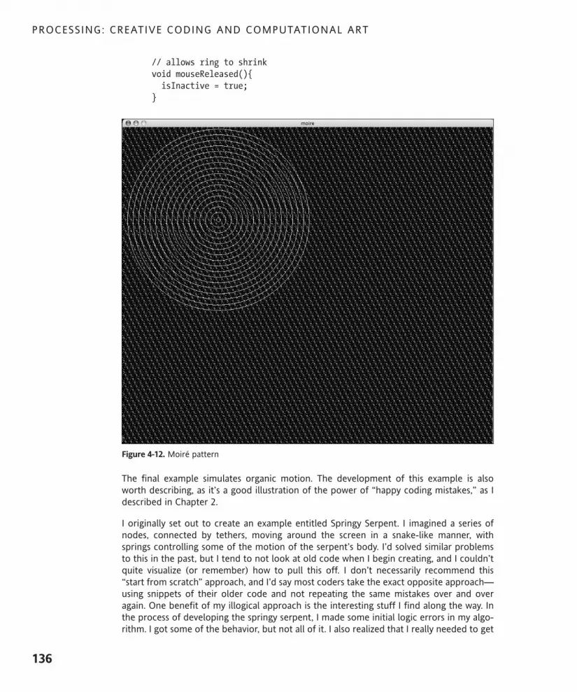
// allows ring to shrinkvoid mouseReleased(){isInactive = true;
}
Figure 4-12. Moiré pattern
The final example simulates organic motion. The development of this example is alsoworth describing, as it’s a good illustration of the power of “happy coding mistakes,” as Idescribed in Chapter 2.
I originally set out to create an example entitled Springy Serpent. I imagined a series ofnodes, connected by tethers, moving around the screen in a snake-like manner, withsprings controlling some of the motion of the serpent’s body. I’d solved similar problemsto this in the past, but I tend to not look at old code when I begin creating, and I couldn’tquite visualize (or remember) how to pull this off. I don’t necessarily recommend this“start from scratch” approach, and I’d say most coders take the exact opposite approach—using snippets of their older code and not repeating the same mistakes over and overagain. One benefit of my illogical approach is the interesting stuff I find along the way. Inthe process of developing the springy serpent, I made some initial logic errors in my algo-rithm. I got some of the behavior, but not all of it. I also realized that I really needed to get
PROCESSING: CREATIVE CODING AND COMPUTATIONAL ART
136
617xCH04.qxd 2/27/07 11:02 AM Page 136

a piece of paper and do a little more involved math to properly solve the problem. Beingimpetuous, manic, and very sleep-deprived, I just kept furiously hacking at the code—hop-ing for some quick (magical) fix; It wasn’t going too well, and I actually went so far as tofind a pencil. Eventually something emerged, but it didn’t look very much like a serpent.Instead, I found a strange, smoky, self-organizing blob (see Figure 4-13). In the end, I thinkI got something more interesting than I originally planned for, and I learned something inthe process—so embrace the chaos! The code to this sketch, entitled Puff, follows. This isnot simple code, but it is an excellent demonstration of the expressive power of trig.
/* puffIra Greenberg, October 22, 2005 */
// for puff headfloat headX;float headY;float speedX = .7;float speedY = .9;
// for puff bodyint cells = 2000;float[]px= new float[cells];float[]py= new float[cells];float[]radiiX = new float[cells];float[]radiiY = new float[cells];float[]angle = new float[cells];float[]frequency = new float[cells];float[]cellRadius = new float[cells];
void setup(){size(400, 400);// begin in the centerheadX = width/2;headY = height/2;
//fill body arraysfor (int i=0; i< cells; i++){radiiX[i] = random(-7, 7); radiiY[i] = random(-4, 4);frequency[i]= random(-9, 9);cellRadius[i] = random(16, 40);
}frameRate(30);
}
void draw(){background(0);noStroke();fill(255, 255, 255, 5);
COMPUTER GRAPHICS, THE FUN, EASY WAY
137
4
617xCH04.qxd 2/27/07 11:02 AM Page 137

//follow the leaderfor (int i =0; i< cells; i++){if (i==0){px[i] = headX+sin(radians(angle[i]))*radiiX[i];py[i] = headY+cos(radians(angle[i]))*radiiY[i];
}else{px[i] = px[i-1]+cos(radians(angle[i]))*radiiX[i];py[i] = py[i-1]+sin(radians(angle[i]))*radiiY[i];
//check collision of bodyif (px[i] >= width-cellRadius[i]/2 || px[i] <= cellRadius[i]/2){radiiX[i]*=-1;cellRadius[i] = random(1, 40);frequency[i]= random(-13, 13);
}if (py[i] >= height-cellRadius[i]/2 || py[i] <= cellRadius[i]/2){radiiY[i]*=-1;cellRadius[i] = random(1, 40);frequency[i]= random(-9, 9);
}}// draw puffellipse(px[i], py[i], cellRadius[i], cellRadius[i]);// set speed of bodyangle[i]+=frequency[i];
}
// set velocity of headheadX+=speedX;headY+=speedY;
//check boundary collision of headif (headX >= width-cellRadius[0]/2 || headX <=cellRadius[0]/2){speedX*=-1;
}if (headY >= height-cellRadius[0]/2 || headY <= cellRadius[0]/2){speedY*=-1;
}}
As always, there are interesting ways to mess with some of the settings in this sketch to getdramatically different results. I utilized Processing’s random() function a lot throughoutthe example. You might remember that the function has two forms and can take eitherone or two arguments. The single-argument function generates a random float valuebetween 0 and the value of the argument. The double-argument version of the functiongenerates a random number between the two argument values. Try messing with thesenumbers to see what happens. Throughout the book, you’ll also look at a bunch of otherinteresting trig experiments, but much more slowly and in detail. There is also a section ontrigonometry in Appendix B of the book.
PROCESSING: CREATIVE CODING AND COMPUTATIONAL ART
138
617xCH04.qxd 2/27/07 11:02 AM Page 138

Figure 4-13. Puff
InteractivityPeople take for granted that when a mouse or other pointing device is connected to theircomputer, the computer will respond to all their wants and desires—or at least clicks.Obviously, the computer needs a little more motivation than that. Mouse presses, releases,hovers, enters, exits, moves, and drags are all loosely classified as mouse events, which canbe further classified more generally as simply events. Event handling is the basis of inter-activity. Events can be mouse behavior, but they can also be window events (resizing a win-dow), keyboard events (pressing a key), menu events (selecting from a pull-down menu),or focus events (selecting a dialog window, palette, or text field as the active area, whichusually then accepts additional input such as filling in a text field with a word). Essentially,any input or state change that the computer can detect can be processed as an event.There are two main aspects to interactivity or working with events: event detection andthe event handling.
Event detectionProcessing and Java have a built-in low-level event detection mechanism, which is a goodthing. If they didn’t, we would be forced to create an endless event loop, constantly check-ing to see if events were occurring. This approach, called polling, is complicated and eatsup CPU cycles (CPU processing time). Part of the reason it is potentially confusing dealswith the very nature of how the computer works. A single-processor machine (with oneCPU) ultimately needs to handle one operation or process at a time. The CPU might be
COMPUTER GRAPHICS, THE FUN, EASY WAY
139
4
617xCH04.qxd 2/27/07 11:02 AM Page 139

able to handle billions of operations per second, but each process is still distinct. The illu-sion that a single computer processor is handling simultaneous events is a function of ourrelatively slow eyes and their inability to see the tiny delays.
Event handling Returning to Processing and Java’s event mechanism, if we don’t need to create our ownloop to detect events, how is it done? Java’s runtime environment, the Java VirtualMachine (JVM), takes care of it for us. In addition, there is an Event class that encapsulatesevent properties and methods. When an event occurs, the Event class detects it and in asense broadcasts it throughout the program. How we receive the broadcast and what wedo with it is mostly what we have to worry about. This efficient system makes event han-dling relatively easy in Java and, as you might suspect, even easier in Processing. Here’s asimple interactive example in which you can click the screen to randomize the sketch. Theevent detection code in the example happens within the if statement in the draw() func-tion, checking the mousePressed condition. When the mouse is pressed, the conditionevaluates to true and the setRandomStyle() function is called.
// click to randomizefloat x, y, squareSize;color bgColor, strokeColor, fillColor;float strokeWt;void setup(){size(400, 400);rectMode(CENTER);x = width/2;y = height/2;setRandomStyle();frameRate(30);
}void draw(){background(bgColor);strokeWeight(strokeWt);stroke(strokeColor);fill(fillColor);rect(x, y, squareSize, squareSize);if (mousePressed){setRandomStyle();
}}void setRandomStyle(){bgColor = color(random(255), random(255), random(255));strokeColor = color(random(255), random(255), random(255));fillColor = color(random(255), random(255), random(255));strokeWt = random(5, 100);squareSize = random(10, 300);
}
PROCESSING: CREATIVE CODING AND COMPUTATIONAL ART
140
617xCH04.qxd 2/27/07 11:02 AM Page 140

Events will be covered and implemented much more in future chapters. If you’d like toplay with another more elaborate interactive example now, download the Tetherballsketch from the code download area on the friends of ED website (www.friendsofed.com/).The sketch includes a fun springing effect, allowing you to drag a bouncy tetherball-likeobject around the screen.
SummaryIf Chapter 3 was a crash course in coding, this chapter has been a crash course in graphicsprogramming. I discussed some general theory as well as a few application areas in thedynamic field of computer graphics. Taking an image apart and looking under the hood atsome low-level graphics processing, you examined the anatomy of computer images downto the pixel level, as well as some of the underlying mathematical and procedural modelsutilized in their creation. You tackled some of the math theory and equations commonlyused in graphics programming, and hopefully you got a sense of the expressive power andcreative potential of some of these relatively simple equations. Finally, you learned a littleabout how interactivity works in Java and Processing. Most of the things covered in thischapter will be revisited throughout the book and expanded upon, so please don’t stressout if you found this chapter overwhelming. I designed it as a general primer, and I realizethat it contains a lot of technical information—not to mention some scary math. I suspectthat some readers will want to periodically come back to this chapter, especially thosetotally new to computer graphics; others might want to review some of the equations orcode examples in Appendix B. In the next chapter, you’ll explore the Processing languageand environment in detail.
COMPUTER GRAPHICS, THE FUN, EASY WAY
141
4
617xCH04.qxd 2/27/07 11:02 AM Page 141

617xCH05.qxd 2/27/07 10:38 AM Page 142

5 THE PROCESSING ENVIRONMENT
617xCH05.qxd 2/27/07 10:38 AM Page 143

Processing, besides being a language of sorts, is an integrated development environment(IDE)—an IDE created by artists for artists. The Processing development environment issimple to learn and use, and doesn’t add to the complexity of learning to program, as withmany other IDEs. In fact, the Processing IDE really does substantially simplify the process ofcoding, even for absolute beginners. Even Flash, which is another very popular IDE of sorts,also geared toward artists, has a steep learning curve, and its complexity can get in the wayon pure coding projects. In contrast, the Processing IDE has a well-designed interface andcore functionality that allows you to work efficiently; it’s a huge improvement over work-ing in your old text editor.
Processing is also a language-specific IDE—a Java IDE—but as you’ll soon see, a prettyunique one. Processing’s seeming simplicity is deceptive, and in one very significant way,Processing goes further than most other IDEs. Processing has its own built-in proceduralprogramming language that enables coders to write Java graphics programs (sketches inProcessing speak) without the complexity or rigid object-oriented structure normallyrequired to write Java. In addition, Processing has three modes of working, allowingcoders, as they increase their programming literacy, to move from Processing’s simplifiedprocedural approach, to a hybrid approach that uses some more-advanced programmingconstructs, to ultimately working in pure Java—all in the same IDE. This multimode capa-bility makes Processing a great environment in which to learn graphics programming, andit’s one of the reasons that it’s being included in more and more digital arts curricula atschools around the world.
In this chapter, I’ll show you how the IDE works, walk you through the features of the envi-ronment, and introduce you to various concepts that are useful to know before you getstarted.
How it worksWhen you double-click the Processing icon, the Processing environment opens up, whichas mentioned is a Java program—technically a Java application. Java applications runthrough a Java interpreter, or Java Virtual Machine (JVM), installed on your computer. TheJVM was either installed with your operating system, as with OS X, or when you installedProcessing (or Java separately), on other platforms. The virtual machine is part of Java’sruntime environment, commonly referred to as the JRE. Java also has a softwaredevelopment kit, or JDK. The JRE includes the JVM, Java’s core classes, and some support-ing files. The JDK includes everything in the JRE, plus a compiler and some additional toolsand files. The JVM installed on your system was built for your specific operating systemand translates or interprets between your compiled Java programs and your specific oper-ating system (OS). What’s cool, or at least efficient, about this approach is that, theoreti-cally, the same code you write on a Mac will run on a Linux or Windows system, with eachof the virtual machines on the different platforms doing the translation at runtime. I wrote“theoretically” because there are some cross-platform display issues, but it essentiallyworks. This cross-platform functionality is one of Java’s strengths, allowing Java to be usedacross different operating systems, as well as on the Web and in other devices—all that isrequired is a JVM.
PROCESSING: CREATIVE CODING AND COMPUTATIONAL ART
144
617xCH05.qxd 2/27/07 10:38 AM Page 144

Returning to Processing—your launched Processing program is being run by the built-inJVM on your computer as a regular Java application. Processing sketches, however, arewritten within the Processing environment, or from within the running Java application.How can the sketches you write be compiled and then launched by Java if Java is alreadybeing used to run the Processing application? This is a good question (if I do say somyself). If you look within the Processing application folder, you’ll notice something calledjikes (see Figure 5-1).
Figure 5-1. Screen capture of the Processing application folder
This is not an exclamation, as in “Holy jikes!” but rather an open source, free Java compilerfrom IBM. Compilers take the higher-level code we humans write and convert it to alower-level language that machines like. In some languages, like C and C++, compilingconverts your program code to a very low-level machine code that is specific to your oper-ating system. So compiling C code on a Mac yields different machine code than compilingthe same code on Windows. However, in Java and Processing, the compiled Java code,called bytecode, will be the same on any platform; and it is the interpreter, or JVM, that isresponsible for translating the bytecode for your specific operating system. If you want tolearn a little more about jikes, check out http://jikes.sourceforge.net/. In the stan-dard JDK from Sun is another complier, javac, which is also free to use, but not opensource.
When you launch the Processing application, which already comes compiled, it’s executed,as I stated before, by the JVM installed on your computer. Your Processing sketches, whichyou write from within the Processing environment, are compiled into Java bytecode (theclass files that the JVM can read) by jikes when you run your sketch. Running your sketchescauses the Processing application to open a new display window, which is a relatively
THE PROCESSING ENVIRONMENT
145
5
617xCH05.qxd 2/27/07 10:38 AM Page 145

simple thing to do, and executes your compiled sketch code within the new display win-dow, all by the same virtual machine. From the virtual machine’s perspective, your sketchis just another process in the larger running program.
Tour de ProcessingFigure 5-2 shows most of the Processing application interface. I didn’t include/expand thetop menu bar, which I’ll cover shortly. You’ll notice, at first glance, that the interface ispretty simple, without extra dialogs, panels, inspectors, and the like cluttering up the envi-ronment. However, the information you need is visible and accessible. Additionally, theenvironment has an intuitive, non-techie look and feel, and doesn’t seem to have a steeplearning curve. As you roll over buttons, you get instant feedback about what they do, inplain simple language (Run, Stop, New, etc.).
PROCESSING: CREATIVE CODING AND COMPUTATIONAL ART
146
Figure 5-2. Screen capture of the Processing application interface
617xCH05.qxd 2/27/07 10:38 AM Page 146

The Processing window is divided into horizontal bands of varying height. I’ll deal witheach, from the bottom up.
The line number, at the very bottom of the window, shows you what line of code you arecurrently working on, based on your cursor position.
The text area gives you verbose feedback about bugs in your code. It can be scary andfrustrating to new coders to see all these errors come up in the text area when they firstbegin coding; rest assured, it happens to all of us. New coders often struggle to even findthe errors in their code, and it can seem impossible that a typo or logic error could stillpossibly exist in code you’ve painstakingly gone through numerous times. The errors willlikely also seem annoyingly cryptic, but over time you’ll learn to understand the messagesand more quickly track down your bugs. However, there are times when even experiencedcoders struggle to eradicate bugs. I usually find taking a break helps (as well as screamingobscenities at the top of my lungs). Eventually, you’ll appreciate these verbose error mes-sages and see how valuable they are in the debugging process. Processing also includestwo commands, print() and println(), that allow you to output information about yoursketch to the text area.
The message area gives you quick feedback during saving and exporting, and tells you inplain, simple language about errors in your code.
The text editor is where you write your sketch code; it’s essentially your old text editor. Ifyou play with it, you’ll notice that there are clear feedback color cues, showing you whatline your cursor is on, what text is selected, and if a word you typed is a legal keyword inthe language.
The tabs show you what files you are working with. Tabs are really handy when your sketchrequires multiple files. At the right side of the tabs area is a right-facing arrow button.Pressing this button opens a pop-up menu that allows you to create and manage yourtabs. When you open an existing sketch in Processing, any Java or PDE files in your sketchdirectory will be automatically put into the tabs layout. The benefit of this will becomeclearer when you begin to work with external functions and classes. By default, there willalways be at least one tab open, with its name at the bottom of the tab pop-up menu. Thistab will be your current main sketch PDE file (it’s called a PDE file because .pde is just thesuffix that Processing sketches use—it stands for “Processing development environment”).As more tabs are created, you’ll see the new tab names at the bottom of the tabs pop-upmenu as well. You can select one of these names by clicking on it to give the tab focus(make it the active window) in the Processing project window. When you click on the tabsarrow button, the pop-up menu allows you to do the following:
Create a new tab
Rename a tab
Delete a tab
Hide/unhide a tab
Move focus to the previous/next tab
THE PROCESSING ENVIRONMENT
147
5
617xCH05.qxd 2/27/07 10:38 AM Page 147

When you create a new tab, you’ll be prompted to give it a name. Processing requires PDEand Java file names to begin with a letter or underscore and contain no spaces. You mayuse numbers in the name after the initial character, and names should be no more than 64characters in length. If you try to name a PDE or Java file using an illegal character,Processing will rename your file automatically, converting the illegal character to anunderscore. For example, the name function 1 will be renamed function_1. In addition,you have the option of adding a .pde or .java suffix. If no suffix is added, Processingassumes the new file is of type PDE. You won’t see the .pde suffix displayed in the tabs, butif you look in your project directory, you’ll see it there. If you specify .java as a suffix, thenthe file should be a standard Java file, and you should see the .java suffix in the tab;although the suffix doesn’t come up at the bottom of the tabs pop-up menu.
Any other suffix you add will be removed and appended to the root of the name, and thefile will be of type PDE. For example, if you accidentally try to save your sketch with thename newfilename.ppe, the full file name will be converted to newfilename_ppe.pde.Again, in the tab, you’ll only see the newfilename_ppe part. Finally, if you hide a tab, itdoes more than just temporarily change the tab’s visibility. When you run or export yourproject, if a tab is hidden, then the file associated with the tab will not be compiled orincluded in the applet subdirectory. The Hide function is a convenient way to ensure thatclasses and functions not being used in your final sketch do not unnecessarily bloat yourprogram when you compile. If you accidentally hide a tab, but still reference it in yourcode, the compiler will give you an error—either “No accessible method,” for a missingfunction; or “Type . . . was not found,” for a missing class. If you look in your sketch direc-tory (see Figure 5-3), you’ll notice that hidden files get appended with .x after the .pde or.java suffix.
Figure 5-3. Screen capture of a Processing sketch directory
PROCESSING: CREATIVE CODING AND COMPUTATIONAL ART
148
617xCH05.qxd 2/27/07 10:38 AM Page 148

The toolbar conveniently contains Processing’s six main control buttons. These buttonsalso have equivalent commands in the menu bar, which I’ll cover a bit later. These are notthe only commands in the Processing application, but they are probably the most oftenused ones. From left to right, these buttons are Run, Stop, New, Open, Save, and Export.The following list describes the functions of each (when applicable, I’ve included the Macand Windows keyboard shortcuts for each in parentheses after the button name):
Run (Cmd+R on OS X; Ctrl+R on Windows): Compiles your code, launches a displaywindow, and executes your sketch within this window.
Stop: Terminates your running program, but leaves the display window open.
New (Cmd+N on OS X; Ctrl+N on Windows): Creates a new sketch within a newproject directory. Both the directory and the PDE file (Processing’s own file format)will share this name. By default, new sketches are saved with the root sketch_, thedate (in the form yy/mm/dd), and a secondary character beginning with the nextalphabetically available character. For example, my current sketch is namedsketch_051024a. If I save this sketch using this name, and then create a new sketch,that sketch will be named sketch_051024b; the next one will be sketch_051024c.Be aware that the default preference state in Processing is to delete emptysketches upon quit. Therefore, if you do not enter any code into the text editorwindow, you will not be able to actually save the project to disk—which I guessmakes sense since there’s nothing to save in the file. If you want to change this set-ting, you can do so in the preferences, found under the Processing menu in OS Xand the File menu in Windows.
Open (Cmd+O on OS X; Ctrl+O on Windows): Displays a menu that lets you choosebetween opening a sketch residing on your local hard drive or across a network,through a standard file navigator; selecting from a list of available sketches, resid-ing within your sketchbook location directory; or loading an example sketch thatcame bundled with the Processing software, from the examples directory residingwithin the main Processing directory. You can set the location of your sketchbook,where the sketches you create will reside, through the preferences—again foundunder the Processing menu in OS X and the File menu in Windows.
Save (Cmd+S on OS X; Ctrl+S on Windows): Writes the current sketch to disk. Youwill not be prompted to confirm that you are writing over the previous state. If youwant to keep your original sketch and also save the current one, you should useSave As, found under File menu. Again, please note that Processing requires sketchnames to begin with a letter or underscore and contain no spaces. You may usenumbers in the sketch name after the initial character, and sketch names should beno more than 64 characters in length. If you try to name a Processing sketch usingan illegal character, Processing will bark at you and rename your file, converting theillegal character to an underscore.
THE PROCESSING ENVIRONMENT
149
5
617xCH05.qxd 2/27/07 10:38 AM Page 149

Export (Cmd+E on OS X; Ctrl+E on Windows): Creates a Java applet of your sketchand places it within an “applet” subdirectory, inside your current sketch directory.Once this subdirectory is created, Processing opens it up for you, displaying fivefiles, which I’ll discuss in a moment. Applets are Java programs that can be viewedin any Java-enabled browser, which includes most modern browsers. Thesebrowsers have a built-in Java interpreter, more commonly known as the JVM. Javaprograms can run as applets or as stand-alone applications on the desktop.However, the source code is not identical for applets and applications, so it doestake a little work to convert an applet to an application and visa versa—that is, ifyou’re not using Processing. Processing includes the ability to export both Javaapplets and stand-alone Java applications.
The applet subdirectory contains these five files:
index.html: The HTML page you load into the browser, with the embeddedapplet.
yourfilename.pde: Your original processing file.
yourfilename.jar: A JAR (Java Archive) file, which is downloaded and run bythe browser’s virtual machine. It contains the Processing core classes, other cus-tom classes, and any media files (images, fonts, etc.) residing within the “data”subdirectory of your sketch directory. Since everything within the subdirectoryis packed into the JAR file when you export, you should remove unneeded datafrom the subdirectory before exporting. If your sketch doesn’t use any externalmedia, you don’t need a data subdirectory.
yourfilename.java: A Java file created by Processing from the main sketch(PDE) file. Java files are compiled by the JVM into bytecode (class files). Theseclass files get packed into the JAR file.
loading.gif: The artwork initially shown as your page loads; it’s replaced by theapplet when it’s loaded.
Finally, if you’re running Processing in OS X, there are three places in which you can alterthe Processing window structure (as shown in Figure 5-2). Some of these adjustments canbe made in Windows as well. You can drag the bar between the text editor and messagearea up and down to resize the window panes. You can resize the entire Processing appli-cation window by dragging the lower-right corner of the window. The “collapse panes”buttons (OS X) work as follows: if the window is in its default state, showing both the texteditor and the message area, clicking the up arrow expands the message area while col-lapsing the text editor, and the down arrow does the opposite.
File menuThis menu is pretty straightforward, and most of it should be self-explanatory. In Figure 5-4,the Sketchbook submenus are exploded. Please note that in Windows, the Processingmenu is contained within the Processing application window, while in OS X, the menu sys-tem is separate from the Processing application. Aside from appearances, the two menuson the different platforms have identical functionality and command sets.
PROCESSING: CREATIVE CODING AND COMPUTATIONAL ART
150
617xCH05.qxd 2/27/07 10:38 AM Page 150

Figure 5-4. Screen capture of Processing’s File ! Sketchbook submenus
The File menu contains the following eight commands:
New (Cmd+N on OS X; Ctrl+N on Windows): This has the same functionality as theNew button on the toolbar.
Sketchbook: The top of the Sketchbook submenu includes the Open command,which has the same functionality as the Open button on the toolbar, discussed pre-viously. Additional content within the Sketchbook submenu includes sketchesyou’ve created, residing at your sketchbook location, specified in the Processingpreferences; and an Examples directory. The Sketchbook submenu checks for PDEfiles, each enclosed within their own directory, within the specified Sketchbookdirectory. The PDE file and its directory must have the same name. You can alsocreate additional outer directories (for organizational purposes) around yourrelated sketches. Processing’s Examples directory, which I’ll discuss in a moment, isorganized this way. PDE files not enclosed within a same-named directory will notbe visible from the Sketchbook submenu. You can still explicitly open them withthe Open command, but Processing will alert you that a directory is required andwill actually create one and move your file into it when you click OK—which ispretty cool. By default, Processing generates this required directory and namingstructure whenever you create a new sketch, so you only need to mess with thisstuff if you really want to. The Examples directory, at the bottom of the Sketchbooksubmenu, is installed with Processing, in the same directory as the Processing appli-cation. It is possible to expand the Examples directory simply by placing your ownsketch examples within it.
THE PROCESSING ENVIRONMENT
151
5
617xCH05.qxd 2/27/07 10:38 AM Page 151

Save (Cmd+S on OS X; Ctrl+S on Windows): This has the same functionality as theSave button on the toolbar.
Save As (Cmd+Shift+S on OS X; Ctrl+Shift+S on Windows): This is similar to theSave function, except that it prompts you for a new sketch name, allowing you tosave the current changed version of your sketch without overwriting the original.
Export (Cmd+E on OS X; Ctrl+E on Windows): This has the same functionality asthe Export button on the toolbar.
Export Application (Cmd+Shift+E on OS X; Ctrl+Shift+E on Windows): This allowsyou to export your sketch as a stand-alone, platform-specific executable applica-tion. Similar to the Export function, Export Application generates an entire directorystructure (in this case, actually three separate directories) with all the required filesto launch an application under Linux, OS X, and Windows. This command alsoopens the current sketch directory, revealing the three newly created applicationdirectories (application.linux, application.macosx, and application.windows).
Page Setup (Cmd+Shift+P on OS X; Ctrl+Shift+P on Windows): This opens the stan-dard Page Setup dialog box to specify printing options. This function has someknown bugs. Please check http://dev.processing.org/bugs/show_bug.cgi?id=435for bug updates.
Print (Cmd+P on OS X; Ctrl+P on Windows): This prints all the code within the maintab or the currently selected tab. This function has some known bugs. Pleasecheck http://dev.processing.org/bugs/show_bug.cgi?id=27 and http://dev.processing.org/bugs/show_bug.cgi?id=28 for bug updates, as well as theProcessing discourse board, at http://processing.org/discourse/yabb_beta/YaBB.cgi, for the most current information about Processing’s printing capabilities.
Edit menuFigure 5-5 shows a screenshot of Processing’s Edit menu.
The Edit menu contains the following eight commands:
Undo (Cmd+Z on OS X; Ctrl+Z on Windows): Cancels the previous action, includingany addition or deletion of code within the text editor. To reverse Undo, select Redo.
Redo (Cmd+Y on OS X; Ctrl+Y on Windows): Reverses the last Undo command,restoring your sketch to the state immediately prior to selecting Undo.
Figure 5-5. Screen capture ofProcessing’s Edit menu
PROCESSING: CREATIVE CODING AND COMPUTATIONAL ART
152
617xCH05.qxd 2/27/07 10:38 AM Page 152

Cut (Cmd+X on OS X; Ctrl+X on Windows): Copies the selected text into clipboardmemory and removes the selected text from the text editor.
Copy (Cmd+C on OS X; Ctrl+C on Windows): Copies the selected text into clip-board memory and leaves the copied text as is within the text editor.
Paste (Cmd+V on OS X; Ctrl+V on Windows): Adds the contents of the clipboardmemory to the text editor window at the cursor’s position, replacing any selectedtext.
Select All (Cmd+A on OS X; Ctrl+A on Windows): Highlights all the text within thetext editor window.
Find (Cmd+F on OS X; Ctrl+F on Windows): Allows you to find and replace key-words within the text editor window. You can replace individual words or allinstances of words, and optionally specify whether searches should be case sensi-tive or not.
Find Next (Cmd+G on OS X; Ctrl+G on Windows): Allows quick and persistentsearches of the last keyword you entered into the Find field. For example, if Iattempt to find the keyword “ball” with the Find command, later on I can simplyselect Find Next, and the next occurrence of the word “ball” will be highlighted inthe text editor. The keyword used by Find Next does not persist between Processingsessions—so if you quit and restart Processing, you’ll lose your keyword in the Findcommand field.
Sketch menuFigure 5-6 shows a screenshot of Processing’s Sketch menu.
Figure 5-6. Screen capture of Processing’s Sketch menu
THE PROCESSING ENVIRONMENT
153
5
617xCH05.qxd 2/27/07 10:38 AM Page 153

The Sketch menu contains the following six commands:
Run (Cmd+R on OS X; Ctrl+R on Windows): Has the same functionality as the Runbutton on the toolbar.
Present (Cmd+Shift+R on OS X; Ctrl+Shift+R on Windows): Creates a full-screendisplay of your executing sketch. The sketch window is centered against a neutralbackground. You can stop the display by selecting the Stop command in the lower-left corner of the screen, or by pressing the Esc key.
Stop: Stops a running sketch.
Import Library: Adds a required import statement to the top of your sketch, allow-ing you to use the classes in the imported code library. The current core Processinglibraries (which can be selected from the Import Library drop-down menu) includethe following:
candy
dxf
javascript
net
opengl
serial
videos
xml
If you select Sketch ! Import Library ! opengl, then the following line of code isadded to the top of your sketch: import processing.opengl.*;. Using importstatements is standard practice in Java, for which related classes of code aregrouped in directories called packages. Packages allow you to organize codelibraries for reuse and distribution. They also provide a way of helping to ensurethat class names don’t collide or interfere with one another. For example, if I cre-ate a class called Ball, and you create a class called Ball, and both of our classesare within a common code library, Java won’t know which one to use. We can solvethis problem by putting each of our classes in a uniquely named package (direc-tory) and then importing the package with the version of the Ball class we need.Then, even if we use both Ball classes, as long as the class files reside in their owndistinctive packages, there will be no naming conflict.
Show Sketch Folder (Cmd+K on OS X; Ctrl+K on Windows): Opens up the directoryof your current sketch. Normally, your current sketch directory will reside withinyour main sketchbook directory. If you remember, your main sketchbook locationis specified in the preferences.
Add File: Opens a file navigator, allowing you to load an image, font, or other mediainto a data subdirectory within your sketch directory. If no data directory exists,Processing will automatically create one for you.
PROCESSING: CREATIVE CODING AND COMPUTATIONAL ART
154
617xCH05.qxd 2/27/07 10:38 AM Page 154

Tools menuFigure 5-7 shows a screenshot of Processing’s Tools menu.
The Tools menu contains the following five commands:
Auto Format (Cmd+T on OS X; Ctrl+T on Windows): This command attempts toformat the code layout for optimal readability. Skipped lines, also referred to aswhitespace, are retained. Syntax errors, such as missing semicolons, are not cor-rected. Auto Format was originally called “beautify,” which is the name of a similarfunction in Processing’s forebear, Design By Numbers (DBN). Here is an example ofhow Auto Format works. If I type the following code into the text editor and selectAuto Format:
void setup(){}void draw(){}
then the code will be reformatted to the following:
void setup(){}void draw(){}
Create Font: One of the challenges of designing for the Web is the incompatibilityof system resources such as installed fonts, which will often be different frommachine to machine and across platforms. One solution is to use only a very lim-ited set of fonts that can be assumed to be installed on most systems—such asArial, Times, and Sans. However, from a design perspective, this is pretty limiting.Another solution is to bundle bitmap glyphs (actual raster graphics of each charac-ter in a font family) with a project to allow the use of fonts that aren’t likely to beinstalled on a user’s machine. The Create Font command does just this. The com-mand opens the Create Font dialog box, which allows you to select any fontinstalled within your system (see Figure 5-8). This dialog includes the options Size,Filename, Smooth (for anti-aliasing), and All Characters. The font generated is a copyof an existing font in your system, created in the VLW font format and installedwithin a data subdirectory in the current sketch directory. Similar to loading othermedia into Processing, a data directory is automatically created, if one doesn’talready exist. There are some memory concerns involved in creating fonts this way.The larger the font size you specify, the more memory the font will use, as eachfont includes the actual raster information needed to draw the individual charac-ters; normally, fonts are created using vector data. In addition, the Smooth optionalso requires a little more memory, as does the All Character option, which includes
Figure 5-7. Screen capture ofProcessing’s Tools menu
THE PROCESSING ENVIRONMENT
155
5
617xCH05.qxd 2/27/07 10:38 AM Page 155
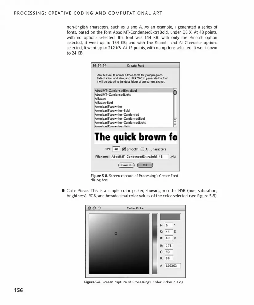
non-English characters, such as ü and Å. As an example, I generated a series offonts, based on the font AbadiMT-CondensedExtraBold, under OS X. At 48 points,with no options selected, the font was 144 KB; with only the Smooth optionselected, it went up to 164 KB; and with the Smooth and All Character optionsselected, it went up to 212 KB. At 12 points, with no options selected, it went downto 24 KB.
Figure 5-8. Screen capture of Processing’s Create Font dialog box
Color Picker: This is a simple color picker, showing you the HSB (hue, saturation,brightness), RGB, and hexadecimal color values of the color selected (see Figure 5-9).
Figure 5-9. Screen capture of Processing’s Color Picker dialog
PROCESSING: CREATIVE CODING AND COMPUTATIONAL ART
156
617xCH05.qxd 2/27/07 10:38 AM Page 156

Copy for Discourse: It is very common for Processing users, especially those cur-rently stuck and/or confused (which happens to all of us), to paste code snippetson the Processing discourse board. Unfortunately, the pasted results don’t alwayslook very good, as some of the formatting gets lost. Some of us with HTML back-grounds simply try inserting HTML tags directly in our code, to fix the formatting—to no avail. The Processing discourse board uses YaBB, a free, open source bulletinboard system. For security reasons, YaBB doesn’t allow the use of HTML tags inposts. Thus, you’re forced to learn yet another proprietary tag system, called YaBBCode (YaBBC) to fix your formatting. Or, you can simply select Copy for Discourse,and Processing will write the YaBBC for you—cool indeed!
Here’s how it works: when you select Copy for Discourse, your sketch code is copiedto your computer’s clipboard and converted into YaBBC for the discourse board;simply paste to the board to recreate your Processing sketch code. In reality, YaBBCis pretty darn close to HTML, so it doesn’t take an experienced coder much time tolearn it—but why waste the brain cells? To learn more about YaBB/YaBBC, visitwww.yabbforum.com/community/YaBB.pl?action=help.
Archive Sketch: This command creates a ZIP archive of the current sketch, prompt-ing you with a Save dialog to choose a location to save the archive.
Help menuFigure 5-10 shows a screenshot of Processing’s Help menu.
Figure 5-10. Screen capture of Processing’s Help menu
The Help menu contains the following:
Getting Started: This launches your default web browser, loading information on theProcessing environment. This functionality does not require an Internet connec-tion, as the information is stored locally within the Processing application directory.The information is divided into three sections. The first, Overview, covers theProcessing development environment, Processing’s three programming modes, andthe different rendering modes. The second section, Platforms, lists the supportedplatforms and some platform-specific information (both the good news and theless-than-good news). One of the nicest aspects of the Processing community is thetransparency and lack of marketing hype when it comes to what Processing can(currently) do and not do. The last section, Export, provides information aboutexporting your sketches as both applets and applications. For the very latest infor-mation, refer to http://processing.org/reference/environment/index.html.
THE PROCESSING ENVIRONMENT
157
5
617xCH05.qxd 2/27/07 10:38 AM Page 157
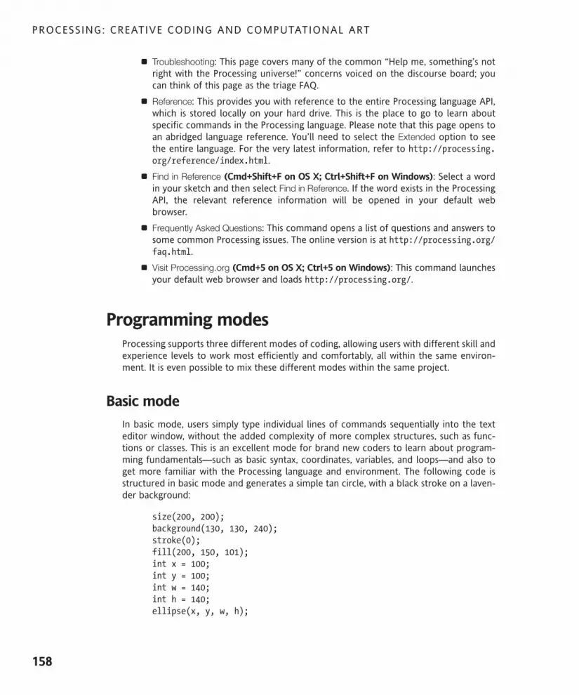
Troubleshooting: This page covers many of the common “Help me, something’s notright with the Processing universe!” concerns voiced on the discourse board; youcan think of this page as the triage FAQ.
Reference: This provides you with reference to the entire Processing language API,which is stored locally on your hard drive. This is the place to go to learn aboutspecific commands in the Processing language. Please note that this page opens toan abridged language reference. You’ll need to select the Extended option to seethe entire language. For the very latest information, refer to http://processing.org/reference/index.html.
Find in Reference (Cmd+Shift+F on OS X; Ctrl+Shift+F on Windows): Select a wordin your sketch and then select Find in Reference. If the word exists in the ProcessingAPI, the relevant reference information will be opened in your default webbrowser.
Frequently Asked Questions: This command opens a list of questions and answers tosome common Processing issues. The online version is at http://processing.org/faq.html.
Visit Processing.org (Cmd+5 on OS X; Ctrl+5 on Windows): This command launchesyour default web browser and loads http://processing.org/.
Programming modesProcessing supports three different modes of coding, allowing users with different skill andexperience levels to work most efficiently and comfortably, all within the same environ-ment. It is even possible to mix these different modes within the same project.
Basic modeIn basic mode, users simply type individual lines of commands sequentially into the texteditor window, without the added complexity of more complex structures, such as func-tions or classes. This is an excellent mode for brand new coders to learn about program-ming fundamentals—such as basic syntax, coordinates, variables, and loops—and also toget more familiar with the Processing language and environment. The following code isstructured in basic mode and generates a simple tan circle, with a black stroke on a laven-der background:
size(200, 200);background(130, 130, 240);stroke(0);fill(200, 150, 101);int x = 100;int y = 100;int w = 140;int h = 140;ellipse(x, y, w, h);
PROCESSING: CREATIVE CODING AND COMPUTATIONAL ART
158
617xCH05.qxd 2/27/07 10:38 AM Page 158
Continuous modeIn continuous mode, users build upon what they’ve learned in basic mode, with the editionof code structures called functions and classes. As you recall, functions are the main build-ing blocks used in procedural programming, and are simply groupings of lines of code thatexecute only when they are explicitly called. Classes are much more complicated struc-tures than functions, and are utilized in OOP. I’ll cover classes in detail in Chapter 8. Inbasic mode, code is executed linearly (line by line). Functions and classes, on the otherhand, allow code to be executed nonlinearly. These structures are only executed whenthey are explicitly called, not when they are initially read into memory.
In continuous mode, two basic Processing functions are provided, which allow you to addyour own custom structures (functions or classes). The two functions are as follows:
void setup(){}
void draw(){}
The setup() function is called only once, at the start of the program. This is the placewhere you normally initialize variables that will be used later in the program. Adding thesetup() function to your sketch allows you to add your own additional custom functionsand classes. The draw() function adds animation capabilities to your sketch and has abuilt-in loop, more accurately called a thread or timer. By default, adding the draw() func-tion to your sketch causes any code between the curly braces of this structure to continu-ously execute. There are a number of ways of controlling this behavior, which I’ll cover inChapter 11. You can also read more about Processing’s draw() function in Appendix A.
The following sketch example is built in continuous mode and uses two custom functions,fadeScreen() and paintOutlines(). The sketch is a little drawing program. I’ve addedcomments throughout the sketch to explain the program flow, although I don’t necessar-ily expect you to fully grasp the code. The sketch allows you to draw by moving and alsodragging the mouse (holding down the mouse button as you move the mouse). A screen-shot of the output of the sketch is shown in Figure 5-11.
/*Drawing ShapesIra Greenberg, November 2, 2005*/
//declare global variablesfloat radiusX, radiusY;
//controls rate of screen fadeint screenFadeValue = 20;
//controls maximum size of shapeint sizeMax = 30;
THE PROCESSING ENVIRONMENT
159
5
617xCH05.qxd 2/27/07 10:38 AM Page 159

//setup structure runs oncevoid setup(){size(400, 400);background(130, 130, 240);noFill();
}
/*draw function begins looprequired by mouseMoved and mouseDraggedfunctions later in the code*/void draw(){}
/*custom function incrementallypaints the screen–called whenthe mouse is pressed*/void fadeScreen(){fill(130, 130, 240, screenFadeValue);noStroke();rect(0, 0, width, height);
}
/*custom function paints shapes,boolean argument 'isDragged' controlsshape style*/void paintShapes(boolean isDragged){if (isDragged){noStroke();ellipse(mouseX, mouseY, radiusX, radiusY);
}else {noFill();stroke(random(255));rect(mouseX, mouseY, random(sizeMax), random(sizeMax));
}}
/* set shape size andfill color on press*/void mousePressed(){// call custom function to clear screenfadeScreen();radiusX = random(sizeMax);radiusY = random(sizeMax);// set fill color for drawingfill(random(255), random(255), random(255), 100);
}
PROCESSING: CREATIVE CODING AND COMPUTATIONAL ART
160
617xCH05.qxd 2/27/07 10:38 AM Page 160

// paint stroked rectanglesvoid mouseMoved(){// call custom functionpaintShapes(false);
}
// paint filled ellipsesvoid mouseDragged(){// call custom functionpaintShapes(true);
}
Figure 5-11. Screen capture of the Drawing Shapes sketch
THE PROCESSING ENVIRONMENT
161
5
617xCH05.qxd 2/27/07 10:38 AM Page 161

Java modeThis mode allows you to work in pure Java, from directly within the Processing text editor.Java mode is extremely flexible, giving you access to the entire Java API. However, thismode is for advanced users who already have a working knowledge of Java. I’ll discussJava mode in more detail in Chapter 14.
Rendering modesProcessing, as of this writing, has three rendering modes: JAVA2D, P3D, and OPENGL. Themode can be explicitly set as an optional argument within Processing’s size() method. Forexample, to use the P3D rendering mode, you would write: size(200, 200, P3D);. Therendering modes control how visual data is rendered, or converted to pixels on the screen.In addition to these three modes, there is a fourth mode, called P2D, that will likely befunctional in the near future (it very well may be active by the time you’re reading this).P2D is an alternative renderer (obviously for 2D rendering) to JAVA2D.
JAVA2D modeJAVA2D uses Java’s 2D graphics library for creating 2D rendering. According to Sun, Java 2Dis “a set of classes for advanced 2D graphics and imaging.” The library contains over 100classes organized into packages according to related functionality (e.g., imaging, drawing,and color). JAVA2D is the default rendering mode in Processing. Thus, when no renderingargument is explicitly specified within the size() function, JAVA2D is used. Coders nor-mally don’t bother adding the JAVA2D argument to the size() call for this reason.
Here is a JAVA2D example that generates a polygon, in this case an octagon. You canchange the value of the sides variable to generate other types of polygons. All the exam-ples in the book thus far have been in JAVA2D mode. Figure 5-12 shows the output of theexample.
/*PolygonIra Greenberg, November 3, 2005*/
// declare variablesint sides = 8; // change to create other polysfloat angle;float radius = 100;float px, py, cx, cy;float[]ptsX= new float[sides];float[]ptsY= new float[sides];
//initialize sketchvoid setup(){size(200, 200, JAVA2D);
PROCESSING: CREATIVE CODING AND COMPUTATIONAL ART
162
617xCH05.qxd 2/27/07 10:38 AM Page 162
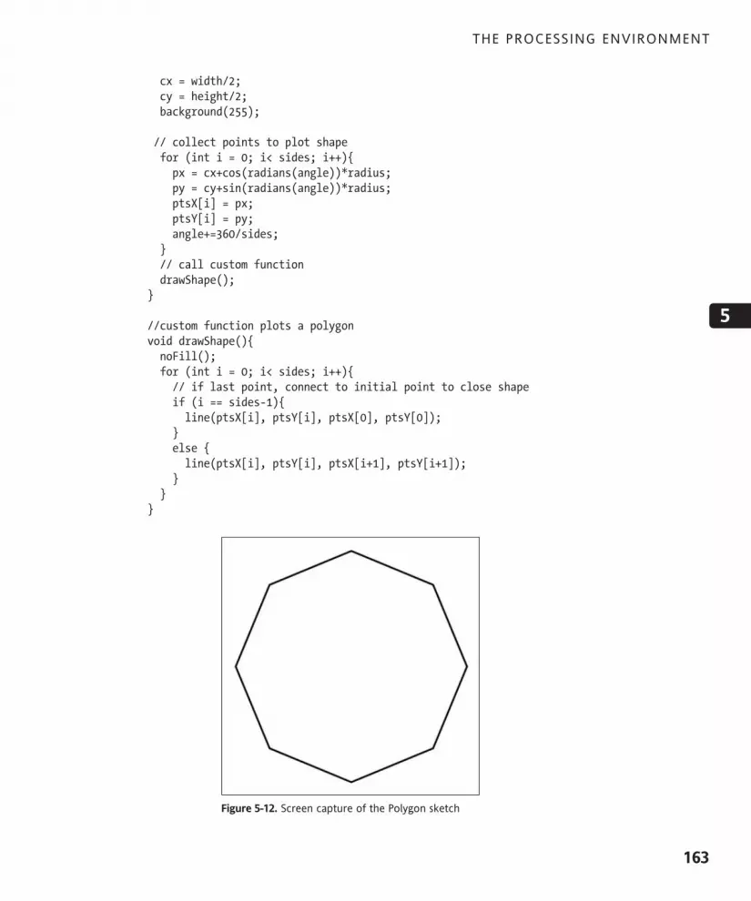
cx = width/2;cy = height/2;background(255);
// collect points to plot shapefor (int i = 0; i< sides; i++){px = cx+cos(radians(angle))*radius;py = cy+sin(radians(angle))*radius;ptsX[i] = px;ptsY[i] = py;angle+=360/sides;
}// call custom functiondrawShape();
}
//custom function plots a polygonvoid drawShape(){noFill();for (int i = 0; i< sides; i++){// if last point, connect to initial point to close shapeif (i == sides-1){line(ptsX[i], ptsY[i], ptsX[0], ptsY[0]);
}else {line(ptsX[i], ptsY[i], ptsX[i+1], ptsY[i+1]);
}}
}
Figure 5-12. Screen capture of the Polygon sketch
THE PROCESSING ENVIRONMENT
163
5
617xCH05.qxd 2/27/07 10:38 AM Page 163

P3D modeP3D mode gives you access to a custom 3D engine in Processing. A 3D engine is just soft-ware (no oil or gears) that allows you to deal with a z-axis, in addition to the standard x- and y-axes. In 3D, geometry is calculated in three dimensions, which is just a simplemath problem for a computer. However, the darn computer screen is only 2D, so theengine has to translate the 3D data back to a 2D screen projection. In the real world, weperceive images decreasing in size as they move farther away from us. We can simulate thisvirtually (both with traditional materials and through software) by using a system ofperspective. I’m sure some of you remember doing simple two and three-point perspec-tive exercises in an intro art class. Perspective works similarly in P3D mode, but without theneed to grab a ruler or get your hands dirty. 3D-to-2D projections on the computer aregenerally tied to the concept of a virtual camera, which is capable of very wide-angle views(in which things are large, close, and often distorted—think fish-eye lens) as well as verydistant views.
Besides virtual camera capabilities, P3D has virtual lights and simple texture mapping(image mapping), allowing an image to be attached to the points (vertices) of 3D geome-try. This capability, called u-v mapping, allows image maps on the geometry to move withthe form. P3D mode is built for speed, a little at the expense of rendering quality.However, P3D mode is a great and relatively easy way to begin experimenting with coding3D with a minimal amount of code and complexity. The following short example rotatesthree concentric polyhedra (polyhedra are basically 3D polygons) and also responds toboth the x and y mouse positions. Figure 5-13 shows the output of the sketch.
/*Rotating PolyhedraIra Greenberg, November 3, 2005*/
//declare variablesfloat rotY;float rotX;
void setup(){size (400, 400, P3D);frameRate(30);
}void draw(){background(255);/* ensures shapes are drawn at thecenter of the display window. In addition,mouse y postion controls the distancethe shapes are drawn along the z-axis.As the shapes moves further into space,they will diminish in size*/translate(width/2, height/2, mouseY-100);
PROCESSING: CREATIVE CODING AND COMPUTATIONAL ART
164
617xCH05.qxd 2/27/07 10:38 AM Page 164

// rotate around Y and X axesrotateY(rotY+=.05);rotateX(rotX+=.1);// mouse x position controls level// of detail of sphere geometrysphereDetail(mouseX/32);fill(0);stroke(255);//draw spheresphere(30);fill(50, 50, 50, 175);noStroke();//draw boxbox(80);noFill();sphereDetail(8);stroke(0);// draw larger outer spheresphere(80);
}
Figure 5-13. Screen capture of the Rotating Polyhedra sketch
THE PROCESSING ENVIRONMENT
165
5
617xCH05.qxd 2/27/07 10:38 AM Page 165

OPENGL modeP3D mode utilizes a software-based 3D engine, meaning that all the 3D calculations arehandled by Java, just as normal 2D calculations are; the 3D math is crunched and con-verted to 2D data before being sent to the graphics hardware to draw the image to thescreen. The hardware isn’t even aware the data began life as 3D geometry. However, yourgraphics hardware has the capability to crunch numbers, and in fact can do it much fasterthan Java. The trick, though, is in communicating directly with the graphics hardware tospeed things up.
OpenGL is a platform-independent library that functions as an interface between yourcode and the graphics hardware. OpenGL was developed in 1992 by Silicon Graphics, butis now overseen by a large group of organizations, under the heading OpenGLArchitecture Review Board. Designed as a set of specifications, OpenGL is platform agnos-tic and can be utilized by practically all systems that have OpenGL-accelerated hardware.Processing and Java interface with OpenGL through JOGL. JOGL, developed by the GameTechnology Group at Sun, is technically considered a Java binding (as in “the ties thatbind”) to OpenGL, and gives Processing sketches that use the OPENGL rendering mode theability to render more stuff faster and at larger sizes. However, to benefit from this mode,you need an OpenGL-accelerated graphics card. Fortunately, most modern machines haveone. To learn more about OpenGL, see www.opengl.org/; and to learn more about JOGL,see https://jogl.dev.java.net/.
Utilizing the OpenGL library couldn’t be simpler in Processing. Simply select Sketch !Import Library ! opengl, which adds an import line to your sketch, and then add theOPENGL string as a third argument to the size function call: size (800, 600, OPENGL);. Thefollowing 3D example (shown in Figure 5-14) can be run in either P3D or OPENGL render-ing mode; simply change the third size argument from OPENGL to P3D. It is worth tryingboth 3D modes to get a sense of how hardware acceleration dramatically impacts per-formance. One word of caution to beginners though: 3D programming is difficult—evenProcessing’s greatly simplified version. If you’re feeling overwhelmed from informationoverload, don’t worry about the 3D renderers. I won’t cover them until the last two chap-ters in the book, at which time you’ll be ready. I do recommend running the example tosee what it does. It’s a little complicated, though, so unless you have prior coding experi-ence, I wouldn’t spend too much time dwelling on it. 3D can be tough, but also prettycool.
/*Space JunkIra Greenberg, November 4, 2005*/
/*need to import opengl library to use OPENGLrendering mode for hardware acceleration*/import processing.opengl.*;
//used for oveall rotationfloat ang;
PROCESSING: CREATIVE CODING AND COMPUTATIONAL ART
166
617xCH05.qxd 2/27/07 10:38 AM Page 166

//cube count-lower/raise to test P3D/OPENGL performanceint limit = 600;
//array for all cubesCube[]cubes = new Cube[limit];
void setup(){//try substituting P3D for OPENGL//argument to test performancesize(800, 550, OPENGL);
//instantiate cubes, passing in random vals for size and postionfor (int i = 0; i< cubes.length; i++){cubes[i] = new Cube(int(random(-20, 20)), int(random(-20, 20)), "int(random(-20, 20)), int(random(-340, 340)), "int(random(-340, 340)), int(random(-340, 340)));
}frameRate(30);
}
void draw(){background(0);fill(200);
//set up some different colored lightspointLight(51, 102, 255, 65, 60, 100);pointLight(200, 40, 60, -65, -60, -150);
//raise overall light in sceneambientLight(70, 70, 10);
/*center geometry in display window.you can change 3rd argument ('0')to move block group closer(+)/further(-)*/translate(width/2, height/2, 150);
//rotate around y and x axesrotateY(radians(ang));rotateX(radians(ang));
//draw cubesfor (int i = 0; i< cubes.length; i++){cubes[i].drawCube();
}//used in rotate function calls aboveang++;
}
THE PROCESSING ENVIRONMENT
167
5
617xCH05.qxd 2/27/07 10:38 AM Page 167

//simple Cube class, based on Quadsclass Cube {
//propertiesint w, h, d;int shiftX, shiftY, shiftZ;
//constructorCube(int w, int h, int d, int shiftX, int shiftY, int shiftZ){this.w = w;this.h = h;this.d = d;this.shiftX = shiftX;this.shiftY = shiftY;this.shiftZ = shiftZ;
}
/*main cube drawing method, which looksmore confusing than it really is. It'sjust a bunch of rectangles drawn foreach cube face*/void drawCube(){beginShape(QUADS);//front facevertex(-w/2 + shiftX, -h/2 + shiftY, -d/2 + shiftZ);vertex(w + shiftX, -h/2 + shiftY, -d/2 + shiftZ);vertex(w + shiftX, h + shiftY, -d/2 + shiftZ);vertex(-w/2 + shiftX, h + shiftY, -d/2 + shiftZ);
//back facevertex(-w/2 + shiftX, -h/2 + shiftY, d + shiftZ);vertex(w + shiftX, -h/2 + shiftY, d + shiftZ);vertex(w + shiftX, h + shiftY, d + shiftZ);vertex(-w/2 + shiftX, h + shiftY, d + shiftZ);
//left facevertex(-w/2 + shiftX, -h/2 + shiftY, -d/2 + shiftZ);vertex(-w/2 + shiftX, -h/2 + shiftY, d + shiftZ);vertex(-w/2 + shiftX, h + shiftY, d + shiftZ);vertex(-w/2 + shiftX, h + shiftY, -d/2 + shiftZ);
//right facevertex(w + shiftX, -h/2 + shiftY, -d/2 + shiftZ);vertex(w + shiftX, -h/2 + shiftY, d + shiftZ);vertex(w + shiftX, h + shiftY, d + shiftZ);vertex(w + shiftX, h + shiftY, -d/2 + shiftZ);
PROCESSING: CREATIVE CODING AND COMPUTATIONAL ART
168
617xCH05.qxd 2/27/07 10:38 AM Page 168

//top facevertex(-w/2 + shiftX, -h/2 + shiftY, -d/2 + shiftZ);vertex(w + shiftX, -h/2 + shiftY, -d/2 + shiftZ);vertex(w + shiftX, -h/2 + shiftY, d + shiftZ);vertex(-w/2 + shiftX, -h/2 + shiftY, d + shiftZ);
//bottom facevertex(-w/2 + shiftX, h + shiftY, -d/2 + shiftZ);vertex(w + shiftX, h + shiftY, -d/2 + shiftZ);vertex(w + shiftX, h + shiftY, d + shiftZ);vertex(-w/2 + shiftX, h + shiftY, d + shiftZ);
endShape();
//add some rotation to each box for pizazz.rotateY(radians(1));rotateX(radians(1));rotateZ(radians(1));
}}
Figure 5-14. Screen capture of the Space Junk sketch
THE PROCESSING ENVIRONMENT
169
5
617xCH05.qxd 2/27/07 10:38 AM Page 169

SummaryThis chapter has looked at the Processing environment in depth, and how its simple, clean,highly functional interface provides an intuitive and friendly environment for new codersand an efficient workspace for seasoned developers. Built on top of Java, Processing uti-lizes a Java interpreter or virtual machine installed within your operating system as well aswithin the browser. Offering three working paths, or programming modes (basic, continu-ous, and Java), Processing supports multiple skill levels and learning styles, all within thesame environment; you can even combine these different approaches in the same sketch.Finally, I covered Processing’s exciting 3D rendering options, including a look at a fast 3Dsoftware engine and the OpenGL library. The next chapter will begin Part 2 of the book,the tutorial-based section that will help you put the theory into practice.
PROCESSING: CREATIVE CODING AND COMPUTATIONAL ART
170
617xCH05.qxd 2/27/07 10:38 AM Page 170

PART TWO PUTTING THEORY INTOPRACTICE
I’ve been looking forward to writing this part of the book—this is the part where youcan focus less on programming theory and language details, and begin playing with thisfascinating medium—which is really what this book is all about. Please try notto worry—if you haven’t quite mastered all the theory and memorized the entireProcessing API, I’ll be revisiting all this in the context of exploring fundamentalaesthetic principles. In the next few chapters, you’ll be using Processing and code as anexperimental, creative medium, not unlike how you would use more traditional mate-rials. In addition, you’ll see how the code medium is distinctive, vis-à-vis other materials,with its own underlying materiality, expressive potential, and aesthetic. This examina-tion will naturally also include concepts of craft, process, and personal expression. Irecommend that you keep the Processing environment open as you work throughthese hands-on chapters, and run the examples as they are covered.
617xCH06.qxd 4/20/07 3:28 PM Page 171

617xCH06.qxd 4/20/07 3:28 PM Page 172

6 LINES
617xCH06.qxd 4/20/07 3:28 PM Page 173

This chapter will concentrate on lines and how they are represented though code. You’llalso look at how lines can represent more multidimensional space, such as shapes andvolume.
It’s all about pointsBefore you can understand a line, you need to move back one dimension and take a lookat points. Here is arguably the simplest graphic program you can write in any language (seeFigure 6-1):
point(50, 50);
Figure 6-1. Single-point sketch
I mentioned before in the book that a point really has no dimension. Wikipedia says ofpoints: “A point in Euclidean geometry has no size, orientation, or any other feature exceptposition.” Thus, your point, as output in Processing, is arguably a tiny square, with a widthand height of a 1 pixel. However, what fun would it be to plot a point that didn’t appear?In fact, your point is really a Processing line, with the same starting and ending points. Thefollowing line function call will yield the same result as the previous point function call:
line(50, 50, 50, 50);
However, this second approach is more complicated than necessary—it’s certainly betterto only have to pass two arguments instead of four—so stick with the point() function.Because point(x, y) is implemented internally with line(x, y, x, y), if you want tochange the color of a point, you need to use the stroke() function, not fill().
There aren’t many things you can do staring at a single static point, other than perhaps sit-ting lotus style and meditating on its oneness—which does have some value. However,enlightenment-seeking aside, let’s add another point (see Figure 6-2):
point(33, 50);point(66, 50);
PROCESSING: CREATIVE CODING AND COMPUTATIONAL ART
174
617xCH06.qxd 4/20/07 3:28 PM Page 174

LINES
175
6
Figure 6-2. Two-point sketch
Adding another point really changes things; it brings up issues of symmetry, balance, andthe gestalt (seeing a face), and begins to suggest a line.
Now add a third point (see Figure 6-3):
point(25, 50);point(50, 50);point(75, 50);
Figure 6-3. Three-point sketch
The line gestalt is certainly getting pretty strong now. The three dots divide top andbottom and have a certain horizontal velocity as your eye sweeps across them.
Now add some code to format the display window, and also add a couple more points (seeFigure 6-4):
size(300, 300);background(0);stroke(255);point(30, 150);point(60, 150);point(90, 150);point(120, 150);point(150, 150);point(180, 150);point(210, 150);point(240, 150);point(270, 150);
617xCH06.qxd 4/20/07 3:28 PM Page 175

PROCESSING: CREATIVE CODING AND COMPUTATIONAL ART
176
Figure 6-4. Emerging line sketch
This is beginning to look like a real program, and it also has an insistent line. There issomething simple and beautiful about the sharpness and delicateness of the white pointsagainst the black. You’ll notice that I called stroke(255), which sets the stroke state ofthe sketch to white. I use the term “stroke state” because any drawing executed after thestroke(255) call that involves rendering a stroke will be white, until I explicitly makeanother call to change the rendering state of the stroke color—for example,stroke(127);. I discuss the idea of a rendering state in the color section of the languagereference, found in Appendix A. The sketch is now 12 lines (of code) long and beginningto get a little unwieldy, especially for making global changes to the program. For example,if you want to now add a tenth point and still keep the line centered in the display win-dow, it’s time-consuming (and annoying) to have to go and change the value for eachpoint. There are two ways to simplify this process. The first is to base your point positionson the size and shape of the display window, and the second is to add a looping structurethat will handle the iteration for you.
Here’s a solution for using ten points, implementing the first improvement:
size(300, 300);background(0);stroke(255);point((width/11)*1, height/2);point((width/11)*2, height/2);point((width/11)*3, height/2);point((width/11)*4, height/2);point((width/11)*5, height/2);point((width/11)*6, height/2);point((width/11)*7, height/2);point((width/11)*8, height/2);point((width/11)*9, height/2);point((width/11)*10, height/2);
This solution is procedurally an improvement—it uses the computer to handle the calcu-lation of the division by 11. Next, I’ll show you how to implement a while loop.
617xCH06.qxd 4/20/07 3:28 PM Page 176

LINES
177
6
Streamlining the sketch with a while loopsize(300, 300);background(0);stroke(255);int i = 1;while (i<11){point((width/11)*i, height/2);i++;
}
This has gotten the sketch down to eight lines. If you really want to, you can shave it fur-ther by a line or two, which I’ll show you shortly. Although the while loop solution isdenser, the reduction in lines of code, I think, makes it more worthwhile than the previoussolution. For example, if you had 100 points, the complexity vs. the convenience clearlywould become an even more palatable trade-off. Before you squeeze the code down yetfurther, I want to go over each line of the sketch to make sure you are following along. Ifthis stuff looks completely unfamiliar, I suspect you began the book after Chapter 3—which is OK. However, I do cover the fundamentals of programming, including loops, indetail in Chapter 3, so you’ll want to review some of this stuff. If you are a seasoned coder,you can probably skip or skim the following description.
Line 1 sets the display size with the function call size(300, 300);. This is a standardProcessing function call, passing two arguments (display window width and display win-dow height). The next two function calls work very similarly, each taking an argument andsetting the background color and the stroke color. You may remember that it is possible toset a background or stroke color with more arguments. For example, background(255,255, 0) creates a yellow background. Next in the sketch I declare and initialize a variablei of type int. Declaring i of the int primitive type means that i can only be assigned inte-ger values. For example, if I try to assign 2.3 to i (i = 2.3;), I’ll get the following compilererror:
The type of the right sub-expression, "float", is not assignable to the variable, of type "int".
Errors like this can be annoying to new coders, but this type checking mechanism is reallythere to help you, so you don’t make a hard-to-find mistake that gets buried in code—which can lead to a much more annoying bug (as well as uncontrolled cussing). The whileloop runs over and over, until some explicit limit is reached. In this case, the while loopwill run as long as i is less than 11. Since i keeps increasing in value, it is also convenientto use i in your programs, as is done in setting the point position calculationpoint(width/11*i, height/2);. The last line in the while loop increments the value of iby 1. If I don’t do this, my loop will never end. Hopefully this seems pretty straightforward.
I mentioned a paragraph or so back that you could still trim a line or two off the sketch;the first way is to increment the counter i within another expression. Here’s the program,one line thinner:
617xCH06.qxd 4/20/07 3:28 PM Page 177

size(300, 300);background(0);stroke(255);int i = 1;while (i<11){point(width/11*i++, height/2);
}
One of the trade-offs of condensing code like this is that the code becomes slightly harderto read. Finally, if you replace with while loop with a for loop, you can also removethe line int i = 1;. Make sure that you also remove the ++ after the i in the point()function call.
Streamlining the sketch further with a for loopsize(300, 300);background(0);stroke(255);for (int i=1; i<11; i++){point(width/11*i, height/2);
}
This is pretty lean now. However, what would make this structure even better and moreusable as a multipurpose code block would be the removal of the number 11, which wecall a “magic number” in programming. Magic numbers are constant values stuck in thecode—usually hastily put in to quickly solve a specific problem. Although they can beeffective hacks or quick fixes, they tend to also be poorly thought-out solutions that don’tlend themselves to code reuse. For example, if you want to now use 100 points, you wouldhave to change the value 11 to 101 in both places in the code. In many programs, therecould be a lot more instances of this value throughout the code. Finally, here’s the sketchthat I might really write (depending on how I was feeling at the moment) to solve thisproblem:
size(300, 300);background(0);int totalPts = 100;float steps = totalPts+1;stroke(255);for (int i=1; i<steps; i++){point((width/steps)*i, height/2);
}
You’ll notice that I actually added two lines of code, but now my sketch can handle anynumber of points. If you raise the totalPts number to over 200, you’ll begin to see a pureline formed from the closely packed points. The line float steps = totalPts+1; seemsto use the magic number 1, and it may seem odd to all of a sudden introduce the float
PROCESSING: CREATIVE CODING AND COMPUTATIONAL ART
178
617xCH06.qxd 4/20/07 3:28 PM Page 178

LINES
179
6
type into the sketch. Although the 1 is a constant, it also expresses a state that is a con-stant. There will always be one more column than the number of points when the pointsare spaced out evenly using outer columns, and one less column than points if outercolumns aren’t used (see Figure 6-5).
Figure 6-5. Calculating columns based on number of objects
The float type keeps rounding errors from shifting the points during division in the forloop. This is a subtle but very important point. For example, the simple expression 5 / 2will not give the answer you might suspect; the answer, in Processing, is 2. This is becausetwo integers are divided together, which returns another integer. To get the right mathe-matical answer (5.0 / 2 = 2.5), one of the operands needs to be a float.
In the sketch, change the float type to int, set totalPts to 30 or 60 points, and run thesketch. Then, set totalPts to 29 or 59 points and run it again; the problem will go away,as 29 + 1 and 59 + 1 yields an even multiple of 300. You can use other values to demon-strate this as well. When steps is declared as type int, and you use it in the for loop (i.e.,(width/steps)*i,), the answer gets rounded to an int. If you want to see the calcula-tions, try putting the statement println((width/steps)*i), within the for loop. You’llsee that all the values are integers. Now switch steps type from int back to float, and theoutput should be real numbers (numbers with fractional parts after the decimal point).
Creating organic form through randomizationOK, so you can draw a line with some points—no big deal, right? Well, there are someinteresting things you can do now that you have your line being described procedurally.For example, to create a more organic or fuzzy line, you can use Processing’s random()function within the loop (see Figure 6-6):
617xCH06.qxd 4/20/07 3:28 PM Page 179

size(300, 300);background(0);int totalPts = 300;float steps = totalPts+1;stroke(255);for (int i=1; i< steps; i++){point((width/steps)*i, (height/2)+random(-2, 2));
}
Figure 6-6. Randomized point line
The function random(-2, 2) generates a random number between the range specified bythe min and max arguments passed to the function. Try passing larger and smaller and alsoasymmetrical arguments to the function to see what happens. Also try changing the num-ber of points. This flexibility and ease with which you can experiment and iterate throughdifferent possibilities is what creative coding is all about. It’s also the reason it’s worth tak-ing the time to code your projects efficiently, using well-structured loops and a minimalamount of magic numbers. Perhaps you’d like the random effect to change over time aswell so that the line is not so consistent. Since the random() function is just looking for twofloat arguments, you can pass those as variables. For example, the following generates aparticle spray (shown in Figure 6-7). Notice I added another variable called rand.
size(300, 300);background(0);int totalPts = 300;float steps = totalPts+1;stroke(255);float rand = 0;for (int i=1; i< steps; i++){point((width/steps)*i, (height/2)+random(-rand, rand));rand+=.2;
}
PROCESSING: CREATIVE CODING AND COMPUTATIONAL ART
180
617xCH06.qxd 4/20/07 3:28 PM Page 180

Figure 6-7. Randomized particle spray
You can even use a random() function to generate values for another random() function.Run the next example a couple of times to see the range of output (one example of whichis shown in Figure 6-8); it’s pretty interesting and getting fairly organic. As always, play withthe numbers to see the expressive potential of the algorithm.
size(300, 300);background(0);int totalPts = 300;float steps = totalPts+1;stroke(255);float rand = 0;for (int i=1; i< steps; i++){point((width/steps)*i, (height/2)+random(-rand, rand));rand+=random(-5, 5);
}
Figure 6-8. Doubly randomized particle line
L INES
181
6
617xCH06.qxd 4/20/07 3:28 PM Page 181

Once you have a single line doing some interesting stuff, you can try to extend the conceptwith multiple lines. One way of thinking of this is as looping a loop. You can pretty easilyput your existing for loop within another for loop and move your line down the displaywindow, repeating the structure over and over again. It is often through these types ofoverlapping iterative processes that really unexpected and interesting stuff starts emergingout of the code. One caution, though: if you’ve been reading this stuff pretty quickly andnot thoroughly experimenting with these structures along the way, you’re missing manyinteresting possibilities, and more importantly, the feature creep in the sketches is going toquickly overwhelm you. I really recommend reading this chapter in small bites and thenthoroughly chewing through the code possibilities. It’s the best way to begin to rememberall the weird syntax and keywords. The next example runs the previous code throughanother outer loop and adds some other modifications, drawing a series of lines down thedisplay window (see Figure 6-9).
/*Razor Tooth PatternIra Greenberg, November 20, 2005*/size(300, 300);background(0);int totalPts = 1000;float steps = totalPts+1;int totalRows = 50; // needs to be < = 300int rowShift = height/totalRows;float rowNudge = -.4;float rowHop = 0;int randNudge = 5;stroke(255);for (int i=rowShift; i<height; i+=rowShift ){for (int j=1; j<steps; j++){rowHop-=rowNudge;if (j % (1 + (int)(random(randNudge))) == 0){rowNudge*=-1;
}point((width/steps)*j, i+rowHop);
}}
PROCESSING: CREATIVE CODING AND COMPUTATIONAL ART
182
617xCH06.qxd 4/20/07 3:28 PM Page 182

LINES
183
6
Figure 6-9. Multiple randomized particle lines
I imagine some of you might need a little clarification on parts of this last example.Although this is a simple program in number of code lines, parts of it are a bit dense.When you nest a for loop, as in the example, it is important to understand how the loopexecutes. The outer for loop initializes i to height/totalRows. This loop will run as longas i is less than the height of the display window. i will be incremented by the sameamount i is originally initialized to, height/totalRows. On the first iteration of the outerfor loop, the inner for loop runs through an entire loop cycle. In this case, j is initializedto 1 and also incremented by 1 as long as it remains less than the value of steps. After theinner loops runs through all its iterations, control goes back to the outer loop, which isincremented by height/totalRows; and then the process repeats itself, with the innerloop again going through its entire iterative loop cycle. This process will continue until thecondition in the outer loop no longer evaluates to true (i is no longer less than the heightof the display window). As you might imagine, if you’re not careful, you can pretty easilycreate nested loops that take a lot of time to finish.
One other significant point regards how you name your variables in the loops. Within acode structure bounded by curly braces (for loops, if statements, functions, etc.), vari-ables declared in the head or body of the structure (or passed in, as in the case of param-eters in the head of a function) have local scope. This is in contrast to variables declaredat the top of a program, which have global scope. Because of local scope, the variable i,declared in the head of the for loop, only exists between the curly braces of the for loop;it has no existence outside the loop. That’s why it’s possible to use the same-named
617xCH06.qxd 4/20/07 3:28 PM Page 183

variable i in all your non-nested for loops. However, when you nest a loop, the inner loopsees all of the variables you created in the outer loop; that’s why you’re forced to use anew name for the loop variable j in the inner loop. If you’ve been following this scopelogic, do you think the outer loop can see the variable declared in the inner loop? Theanswer is no because the rules of local scope still apply.
Getting back to the code example, within the inner loop are a few lines that might beconfusing:
rowHop-=rowNudge;if (j % (1+ (int)(random(randNudge))) == 0){rowNudge*=-1;
}
The first line is a standard shortcut assignment operation. The variable rowHop moves thepoints up and down on the y-axis, and rowNudge is the value that it’s either incremented ordecremented by. I use the term “shortcut” because this operation does both an arithmeticoperation (subtraction) and an assignment operation. The next line uses the modulusoperator, which is usually foreign to non-coders. Modulus returns the remainder of divi-sion between two operands. The reason I used it was to generate a somewhat randomresult in the loop. I tested for the modulus expression to evaluate to 0, meaning that thedivision would yield no remainder. As i increases, there is a greater possibility that divisionwill have no remainder. For example, 4 has three factors (1, 2, and 4) that go into it evenly,but 12 has six (1, 2, 3, 4, 6, and 12). In addition, I used a random number generator for theright operand to make the process more chaotic. The reason I added 1 to the value of therandom() function before doing the modulus operation was to avoid division by 0, whichis illegal and will cause a compiler error. Since the random() function will generate a ran-dom value between 0 and the argument value, periodically 0 will come up. In addition, Iam converting the float value, evaluated by the random() function, to an integer, so themodulus expression has a chance of evaluating to 0. When you convert a float to an intby using the int() function, values are rounded down, so .999 still evaluates to 0. Thus,the statement (int)(random(randNudge)) can generate a lot of zeros. I used parenthesesaround the entire expression (1 + (int)(random(randNudge))) to make sure that theaddition happens before the division. Normally multiplication and division, including mod-ulus, are evaluated before addition and subtraction, but you can use parentheses tochange the order of precedence, which is discussed at more length in Chapter 3. Finally,the shortcut assignment operation rowNudge*=-1; switches the direction in which thestatement rowHop-=rowNudge; is pushing the points on the y-axis, giving a razor-tooth pat-tern to the line output. Hopefully this description wasn’t too rough on the head. Makesure you play, tweak, experiment, and bust apart the code to get a better sense of what’sgoing on.
There are two more modifications I’ll make to the current sketch, and then I’ll (finally)move on to using Processing’s “real” line functions. The first modification involves laying amore regular grid pattern on top of the razor-tooth pattern, and the second modificationinvolves shifting value.
PROCESSING: CREATIVE CODING AND COMPUTATIONAL ART
184
617xCH06.qxd 4/20/07 3:28 PM Page 184

Coding a gridTo begin, I’ll show you how to generate a simple grid. First, you’ll generate some columnsof equally spaced parallel points (see Figure 6-10). This code should look similar to whatyou’ve been doing thus far.
size(300, 300);background(0);int cellWidth = width/30;stroke(255);//vertical linesfor (int i=cellWidth; i<width; i+=cellWidth){for (int j=0; j<height; j++){point(i, j);
}}
Figure 6-10. Vertical lines generated from points
L INES
185
6
617xCH06.qxd 4/20/07 3:28 PM Page 185

If you mess with the cellWidth variable, you can change the spacing frequency. Now let’sadd the horizontal lines (see Figure 6-11):
size(300, 300);background(0);int cellWidth = width/20;int cellHeight = height/30;stroke(255);//vertical linesfor (int i=cellWidth; i<width; i+=cellWidth){for (int j=0; j<height; j++){point(i, j);
}}//horizontal linesfor (int i=cellHeight; i<height; i+=cellHeight){for (int j=0; j<width; j++){point(j, i);
}}
Figure 6-11. Horizontal and vertical lines, forming a symmetrical grid, generated from points
PROCESSING: CREATIVE CODING AND COMPUTATIONAL ART
186
617xCH06.qxd 4/20/07 3:28 PM Page 186

Notice that you can make the value of cellWidth different than the value of cellHeight,creating an alternative grid (see Figure 6-12). Finally, let’s add some random() functionsthroughout the program.
Figure 6-12. Alternative grid made from points
One of the advantages of generating a line this way, using adjacent points, is the ability toalter the spacing of the points, as in the next example (see Figure 6-13):
/*Point GridIra Greenberg, November 20, 2005*/size(300, 300);background(0);// grid variablesint cellWidth = width/20;int cellHeight = height/20;int ptGap = 3;int randHt = 4;int randWdth = 10;stroke(255);//vertical linesfor (int i=cellWidth; i<width; i+=cellWidth+int(random(randWdth))){
LINES
187
6
617xCH06.qxd 4/20/07 3:28 PM Page 187

for (int j=0; j<height; j+=ptGap){point(i, j);
}}//horizontal linesfor (int i=cellHeight; i<height; i+=cellHeight+int(random(randHt)) ){for (int j=0; j<width; j+=ptGap){point(j, i);
}}
Figure 6-13. Alternative grid with spaced-out points
Now that you have your grid, let’s bring the razor-tooth code back and put the two pat-terns together, as shown in Figures 6-14 and 6-15:
/*Yin YangIra Greenberg, November 20, 2005*/size(300, 300);background(0);//razor tooth variablesint totalPts = 1000;
PROCESSING: CREATIVE CODING AND COMPUTATIONAL ART
188
617xCH06.qxd 4/20/07 3:28 PM Page 188
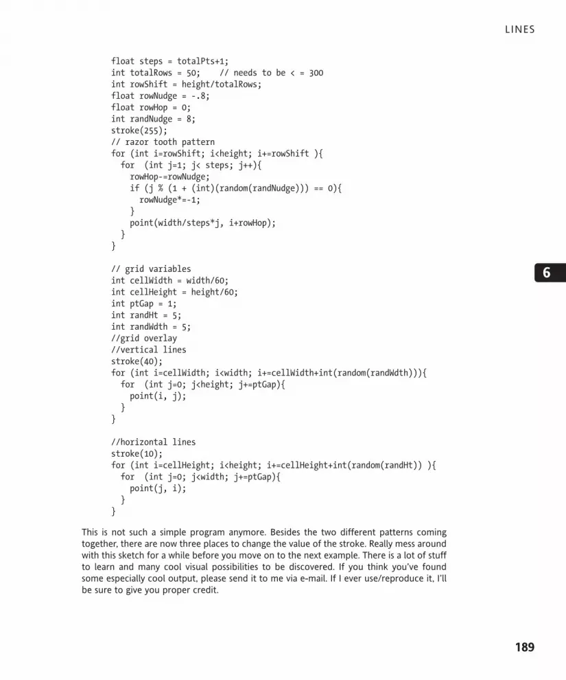
float steps = totalPts+1;int totalRows = 50; // needs to be < = 300int rowShift = height/totalRows;float rowNudge = -.8;float rowHop = 0;int randNudge = 8;stroke(255);// razor tooth patternfor (int i=rowShift; i<height; i+=rowShift ){for (int j=1; j< steps; j++){rowHop-=rowNudge;if (j % (1 + (int)(random(randNudge))) == 0){rowNudge*=-1;
}point(width/steps*j, i+rowHop);
}}
// grid variablesint cellWidth = width/60;int cellHeight = height/60;int ptGap = 1;int randHt = 5;int randWdth = 5;//grid overlay//vertical linesstroke(40);for (int i=cellWidth; i<width; i+=cellWidth+int(random(randWdth))){for (int j=0; j<height; j+=ptGap){point(i, j);
}}
//horizontal linesstroke(10);for (int i=cellHeight; i<height; i+=cellHeight+int(random(randHt)) ){for (int j=0; j<width; j+=ptGap){point(j, i);
}}
This is not such a simple program anymore. Besides the two different patterns comingtogether, there are now three places to change the value of the stroke. Really mess aroundwith this sketch for a while before you move on to the next example. There is a lot of stuffto learn and many cool visual possibilities to be discovered. If you think you’ve foundsome especially cool output, please send it to me via e-mail. If I ever use/reproduce it, I’llbe sure to give you proper credit.
L INES
189
6
617xCH06.qxd 4/20/07 3:28 PM Page 189
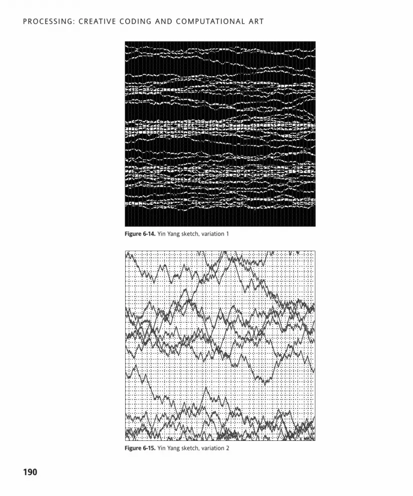
PROCESSING: CREATIVE CODING AND COMPUTATIONAL ART
190
Figure 6-14. Yin Yang sketch, variation 1
Figure 6-15. Yin Yang sketch, variation 2
617xCH06.qxd 4/20/07 3:28 PM Page 190

LINES
191
6
Creating space through fadesYour last modification will be shifting the value of the stroke. Since color is representednumerically, you can easily shift the color’s value/chroma just by applying some calcula-tions to the color’s numeric value. Going back to the vertical lines example, here’s theoutput fading to black. Notice how it feels like the form goes back into space (seeFigure 6-16).
size(300, 300);background(0);float cellWidth = width/30.0;// find ratio of value range(255) to widthfloat val = cellWidth*(255.0/width);//vertical linesfor (float i=cellWidth, v=255; i<width; i+=cellWidth, v-=val){stroke(v);for (int j=0; j<height; j++){point(i, j);
}}
Figure 6-16. Horizontal fade to black
617xCH06.qxd 4/20/07 3:28 PM Page 191

There is one new concept in this example and a little mathematical expression that mayneed some clarification. The expression that might be problematic is the following:
float val = cellWidth*(255.0/width);
I need the decrementation of the color value to coincide with the number of steps in thefor loop. To ensure that this happens, I need to find the ratio between the width ofthe display window and the maximum value of the color (255). I simply multiply this ratioby the cellWidth interval to calculate how much to decrement the color value each stepof the loop. This gives me a smooth transition from 255 to 0 (or white to black). The newconcept I mentioned refers to using multiple statements within the head of the for loop,separated by commas. This is a convenient thing to do. I could also have initialized a vari-able outside of the loop and explicitly incremented/decremented it within the loop block,but that’s more work. In truth, all three parts in the head of the for loop are optional (youdo need the semicolons, though). For example, this for loop will compile and run fine. Iused the break; command so that the loop doesn’t run infinitely.
for(;;){print("i'm in this weird for loop");break;
}
In the next modification, I applied the value shifting to both the vertical and horizontallines (see Figure 6-17). I also broke out of the square format to illustrate how the grid canautomatically size itself to the display window size/format. This is a good example ofwhy you want to try to base program measurements (if it’s at all practical) on the dimen-sions of the display window, which allows your program to scale and adapt to differentenvironments.
size(500, 200);background(0);float cellWidth = width/50.0;// find ratio of value range(255) to widthfloat valw = cellWidth*(255.0/width);//vertical linesfor (float i=cellWidth, v=255; i<width; i+=cellWidth, v-=valw){stroke(v);for (int j= 0; j<height; j++){point(i, j);
}}
float cellHeight = height/50.0;// find ratio of value range(255) to heightfloat valh = cellHeight*(255.0/height);//horizontal linesfor (float i=cellHeight, v=255; i<height; i+=cellHeight, v-=valh){stroke(v);
PROCESSING: CREATIVE CODING AND COMPUTATIONAL ART
192
617xCH06.qxd 4/20/07 3:28 PM Page 192

LINES
193
6
for (int j=0; j<width; j++){point(j, i);
}}
Figure 6-17. Horizontal and vertical fade to black
The last thing I’ll do with the beleaguered point method is combine the gradient strokegrid with the razor-tooth pattern. Two examples of the sketch’s output can be seen inFigures 6-18 and 6-19.
/*Yin Yang FadeIra Greenberg, November 20, 2005*/size(700, 200);background(0);
// grid variablesfloat cellWidth = width*.01;float cellHeight = height*.01;int ptGap = 1;int randHt = 0;int randWdth = 0;// find ratio of value range(255) to height and widthfloat valh = cellHeight*(255.0/height);float valw = cellWidth*(255.0/width);
//grid overlay//vertical linesfor (float i=cellWidth, v=255.0; i<width; i+=cellWidth + !
int(random(randWdth)), v-=valw ){stroke(v);for (int j=0; j<height; j+=ptGap){
617xCH06.qxd 4/20/07 3:28 PM Page 193

PROCESSING: CREATIVE CODING AND COMPUTATIONAL ART
194
point(i, j);}
}//horizontal linesfor (float i=cellHeight, v=255.0; i<height; i+=cellHeight + !
int(random(randHt)), v-=valh ){stroke(v);for (int j=0; j<width; j+=ptGap){point(j, i);
}}
//razor tooth variablesfloat totalPts = 1000.0;float steps = totalPts+1.0;int totalRows = 50; // needs to be < = 300int rowShift = height/totalRows;float valr = 255.0/steps; // used for value shiftfloat rowNudge = -.7;float rowHop = 0;int randNudge = 8;// razor tooth patternfor (int i=rowShift; i<height; i+=rowShift ){for (float j=1, v=255; j< steps; j++, v-=valr){stroke(v);rowHop-=rowNudge;if (j % (1 + (int)(random(randNudge))) == 0){rowNudge*=-1;
}point(width/steps*j, i+rowHop);
}}
Figure 6-18. Yin Yang Fade sketch, variation 1
617xCH06.qxd 4/20/07 3:28 PM Page 194
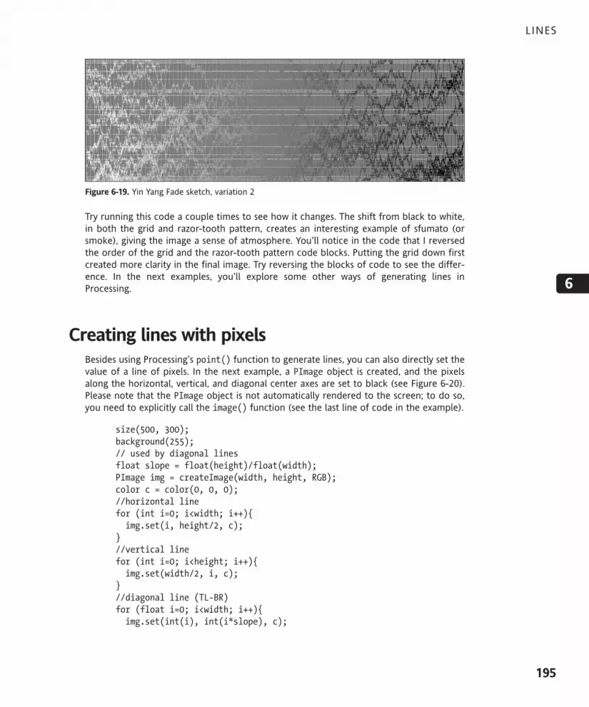
Figure 6-19. Yin Yang Fade sketch, variation 2
Try running this code a couple times to see how it changes. The shift from black to white,in both the grid and razor-tooth pattern, creates an interesting example of sfumato (orsmoke), giving the image a sense of atmosphere. You’ll notice in the code that I reversedthe order of the grid and the razor-tooth pattern code blocks. Putting the grid down firstcreated more clarity in the final image. Try reversing the blocks of code to see the differ-ence. In the next examples, you’ll explore some other ways of generating lines inProcessing.
Creating lines with pixelsBesides using Processing’s point() function to generate lines, you can also directly set thevalue of a line of pixels. In the next example, a PImage object is created, and the pixelsalong the horizontal, vertical, and diagonal center axes are set to black (see Figure 6-20).Please note that the PImage object is not automatically rendered to the screen; to do so,you need to explicitly call the image() function (see the last line of code in the example).
size(500, 300);background(255);// used by diagonal linesfloat slope = float(height)/float(width);PImage img = createImage(width, height, RGB);color c = color(0, 0, 0);//horizontal linefor (int i=0; i<width; i++){img.set(i, height/2, c);
}//vertical linefor (int i=0; i<height; i++){img.set(width/2, i, c);
}//diagonal line (TL-BR)for (float i=0; i<width; i++){img.set(int(i), int(i*slope), c);
LINES
195
6
617xCH06.qxd 4/20/07 3:28 PM Page 195

}//diagonal line (BL-TR)for (float i=0; i<width; i++){img.set(int(i), int(height-i*slope), c);
}image(img, 0, 0);
Figure 6-20. Drawing lines with pixels example
This approach is pretty low level for simply drawing some lines, and isn’t much of animprovement (if any) over using the point() method. I’ll return to PImage later in thebook. However, one detail worth noting in the last example is the simple equation used togenerate the diagonal lines. Since the lines were set by incrementing pixels across theimage, I needed to the know the slope of the lines I wanted to draw, which is really howthe line changes on the y-axis in regard to how it changes on the x-axis. The stroke equa-tion is just the change in y divided by the change in x (the rise over the run). Normally fora line, you just take the beginning and ending points, do the subtraction between the twoy and x components, and then perform the division. Since in the example the diagonallines span the entire display window (from corner to corner), I could just use the displaywindow height divided by the width to get my slope.
Processing’s line functionsFortunately, Processing has two other far more simplified approaches to generating linesthat also give you more rendering capabilities, such as setting the weight or thickness ofthe line. The first approach you’ll look at uses Processing’s line() function. This functioncomes in two varieties, 2D and 3D. The 3D version works just like the 2D function, butrequires six arguments instead of four. These arguments are the x and y (and for 3D, also z)
PROCESSING: CREATIVE CODING AND COMPUTATIONAL ART
196
617xCH06.qxd 4/20/07 3:28 PM Page 196

coordinates of the line. For example, to draw a 2D line across the screen, you pass the ini-tial point’s coordinate, (x1, y1), and the endpoint’s coordinate, (x2, y2), to the line(x1,y1, x2, y2) function. Figure 6-21 shows the output.
size(500, 300);background(255);line(0, height/2, width, height/2);
Figure 6-21. Drawing a 2D line with Processing’s line() function
If you were using one of the 3D rendering options (P3D or OPENGL), you could pass in athird coordinate, referencing the z-axis. If you run the next example, you’ll notice that theline doesn’t appear to reach the end of the display, as it did in the last example. Thisis because the line is stretching back 300 pixels into virtual space, and the P3D renderer issimulating perspective, which causes things to converge and decrease in scale (visually ofcourse) as they recede into space (see Figure 6-22).
size(500, 300, P3D);background(255);// line(x1, y1, z1, x2, y2, z2);line(0, height/2, 0, width, height/2, -300);
Figure 6-22. Drawing a 3D line with Processing’s line() function
L INES
197
6
617xCH06.qxd 4/20/07 3:28 PM Page 197

The rest of the examples in this chapter will be 2D. (Drawing in 3D will be discussed laterin the book.) Utilizing the line() function, you can more easily create complex linearstructures than using either the point() or PImage approaches. Aside from specifying theposition and length of a line, you can use some of Processing’s rendering style functions toaffect the rendering state of the line. Next is a very simple example demonstrating the useof the strokeWeight() function (see Figure 6-23).
size(500, 300);background(255);int step = height/10;for (int i=step; i< height; i+=step ){strokeWeight(i*.1);line(20, i, width-20, i);
}
Figure 6-23. Stroke weight variation example
As the line or stroke increases in weight, the end caps of the line become very prominent.The default style is ROUND. However, end caps can be set using the strokeCap() functionby passing one of three constants, ROUND, PROJECT, or SQUARE, to the function. I recodedthe last example, changing some of the end caps (see Figure 6-24). Please also note thestrokeCap() function only works with the default JAVA2D rendering mode. If you specifyany of the other modes (P3D, OPENGL, or P2D), this feature will not work.
size(500, 300);background(255);int step = height/10;int[]caps = {ROUND, PROJECT, SQUARE};int j = 0;for (int i=step; i<height; i+=step ){strokeWeight(i*.1);strokeCap(caps[j++]);if (j>2){j=0;
}line(20, i, width-20, i);
}
PROCESSING: CREATIVE CODING AND COMPUTATIONAL ART
198
617xCH06.qxd 4/20/07 3:28 PM Page 198

LINES
199
6
Figure 6-24. End cap variation example
Running this code should give you a clear sense of the differences between the end capstyles. These caps become a more significant concern as you begin to join lines into morecomplex structures. However, before you do that, let’s review some of the code in the lastexample.
The line int[]caps = {ROUND, PROJECT, SQUARE}; declares and initializes an array of typeint, and fills the index positions [0], [1], and [2] with the three constants ROUND,PROJECT, and SQUARE. I discussed arrays in detail in Chapter 3. As a review, arrays are datastructures that hold multiple variables of any type. All the elements in an array need to beof the same data type. To access an item stored in an array, you use an index numberplaced between brackets, directly to the right of the array name, as in caps[0]. Arrays arezero-indexed, meaning that the first position in the array is 0, not 1. The three end capstyles, ROUND, PROJECT, and SQUARE, which look like strings, are actually immutable(unchangeable) integer constants. Specifying an unchanging value as a constant and usingall uppercase letters in naming it are common programming approaches. In Java, the key-word final is used to specify that a variable’s value is immutable. To find the correspon-ding int values for the constants, run the following example:
println("ROUND = " + ROUND);println("SQUARE = " + SQUARE);println("PROJECT = " + PROJECT);// uncomment the next line to generate a semantic error.//ROUND = 27;
Now, to prove that you can’t change a constant’s value, uncomment the last line of thecode and run the sketch again, which should generate a compiler error telling you can’tassign another value to ROUND.
Processing has a ton of constants defined in the language that work the same way. Eachconstant is usually assigned an integer value (but not always). Mostly, constants add mean-ing to the coding process. Isn’t it easier to remember the cap style ROUND than the number2? You can see Processing’s constants at http://dev.processing.org/source/index.cgi/trunk/processing/core/src/processing/core/PConstants.java?view=markup.
617xCH06.qxd 4/20/07 3:28 PM Page 199

Joining linesIn the previous example, I also used a conditional statement to keep looping through thecaps arrays. Since each end cap was output three times, I needed to keep resettingthe array counter back to 0, which is exactly what the conditional statement does:
if (j>2){j=0;
}
The next sketch, shown in Figure 6-25, illustrates the joining implications of the differentend caps. In addition, the sketch implements a column layout algorithm, with simplepadding between the corresponding cells. Try changing the value of the strokeWeight()argument as well as the shapes and padding variables to see what happens.
/*Auto LayoutIra Greenberg, November 21, 2005*/size(500, 300);background(255);int[]caps = {ROUND, PROJECT, SQUARE};strokeWeight(20);int shapes = 3;int padding = 200;
float w = (width-padding)/shapes;float h = w;float colSpan = (width-shapes*w)/(shapes+1);float x = colSpan;float y = height/2-h/2;for (int i=0, j=0; i<shapes; i++){strokeCap(caps[j++]);if (j>2) j=0;line(x, y, x+w, y);line(x+w, y, x+w, y+h);line(x, y+h, x+w, y+h);line(x, y+h, x, y);x+=w+colSpan;
}
PROCESSING: CREATIVE CODING AND COMPUTATIONAL ART
200
617xCH06.qxd 4/20/07 3:28 PM Page 200

Figure 6-25. Auto Layout sketch
This sketch utilizes a fair amount of variables, so it might look a bit confusing. Definitelytake your time going through it. I think the auto-layout feature is worth taking the time tounderstand, as this type of process is quite valuable when you’re doing visual stuff. You’llalso notice that I initialized a second local variable (j) in the for loop head, which I use tocycle through the caps[] array. There is also a conditional statement that keeps resettingj to 0, ensuring that the index of the array stays within bounds. Remember, arrays arezero-indexed—so if you have three items in an array, the last index number will be 2, orarray.length-1. If you make a request to access an index position in an array that doesn’texist, you’ll get an error. This is a very common mistake, and usually pretty easily (andhappily) resolved.
I also snuck in some formatting that hopefully will look quite suspect: if (j>2) j=0;. Thisis actually a normal conditional statement that I put on one line, leaving off the curlybraces. Yes, this is legal code, as long as you only use one statement in the block of thecode (between where the curly braces would have been). You can even use an else state-ment after the if block—but again, only one line of code will be recognized by the struc-ture if you don’t include curly braces. You’ll also get a compiler error if you include theelse and have more than one line in the if block. Regardless of how you format your ifstatement, it makes no difference whether you put it on one line or skip a line betweeneach part (at least to the compiler). Whitespace is ignored by the compiler, except if it’sbetween quotation marks, which it then sees as character spaces. In the next examples, thefirst two snippets works fine, but the last two don’t work.
Here’s Example 1, which works:
for (int i =0; i<5; i++){// no braces, but only one line in both the if and else blocksif (i==3)println("i = " + i + " hello");
elseprintln("i = " + i + " goodbye");
}
LINES
201
6
617xCH06.qxd 4/20/07 3:28 PM Page 201

Example 2 also works, but looks pretty ridiculous.
for(int i=0;i<5;i++){if (i==3)println(" hello");elseprintln("goodbye");}
Example 3 doesn’t work properly (although it will compile and run fine). If you run thecode, you’ll notice that the second line in the if block (below the comment) outputs eachiteration of the loop, regardless of whether the conditional statement is true—this a greatway to create a hard-to-track-down and really annoying bug.
for (int i=0; i<5; i++){if (i==3)print("i = " + i + " hello");/* Without using curly braces, the next line will always execute,
regardless of the outcome of the conditional (true or false)*/println(" there");
}
Example 4 won’t even compile, which is a good thing:
for (int i=0; i<5; i++){if (i==3)print("i = " + i + " hello");println(" there");
elseprint("i = " + i + " goodbye");
}
In spite of this flexibility in form, I almost always use curly braces and format my state-ments on multiple lines. However, there are many coders who use these other forms, soit’s good to be able to recognize them and, most importantly, recognize when they’ll workproperly or not.
Creating a table structureSince you’ve got the auto-format code working for columns, let’s set it up for rows as well,and then let’s try to do something visually interesting with it (see Figure 6-26).
/*Table Layout IIra Greenberg, November 21, 2005*/size(500, 300);background(255);int[]caps = {ROUND, PROJECT, SQUARE};strokeWeight(1);int cols = 30;int rows= 40;
PROCESSING: CREATIVE CODING AND COMPUTATIONAL ART
202
617xCH06.qxd 4/20/07 3:28 PM Page 202

int xPadding = 150;int yPadding = 100;float w = (width-xPadding)/cols;float h = (height-yPadding)/rows;float colSpan = (width-cols*w)/(cols+1);float rowSpan = (height-rows*h)/(rows+1);float x;float y = rowSpan;for (int i=0; i<rows; i++){x = colSpan;for (int j=0, k=0; j<cols; j++){strokeCap(caps[k++]);if (k>2){
k=0;}line(x, y, x+w, y);line(x+w, y, x+w, y+h);line(x, y+h, x+w, y+h);line(x, y+h, x, y);x += w+colSpan;
}y+=h+rowSpan;
}
Figure 6-26. Table Layout I sketch
You’ve got a nice, flexible table structure now. Running the sketch, you should see a tightlypacked pattern of small rectangles. Try decreasing the padding and increasing/decreasingthe stroke weight. Since your table doesn’t need to hold well-formatted tabular data, youcan do “stupid” but fun things to it (the theme of my life). For example, what does
L INES
203
6
617xCH06.qxd 4/20/07 3:28 PM Page 203

PROCESSING: CREATIVE CODING AND COMPUTATIONAL ART
204
negative padding do to the table structure? You can also make things more interestingby adding randomization directly into the plotting algorithm. Your table will then go froman array of cells or windows to (potentially) many little individual works of art (seeFigure 6-27).
/*Table Layout IIIra Greenberg, November 21, 2005*/void setup(){size(700, 500);background(0);drawTable();
}
void drawTable(){stroke(255);int[]caps = { ROUND, PROJECT, SQUARE };strokeWeight(.1);int cols = 20;int rows= 20;int xPadding = 100;int yPadding = 100;float w = (width-xPadding)/cols;float h = (height-yPadding)/rows;float colSpan = (width-cols*w)/(cols+1);float rowSpan = (height-rows*h)/(rows+1);float x;float y = rowSpan;for (int i=0; i<rows; i++){x = colSpan;for (int j=0, k=0; j<cols; j++){strokeCap(caps[k++]);if (k>2){k=0;
}line(x+random(-4, 4), y+random(-4, 4), x+w+random(-4, 4), !
y+random(-4, 4));line(x+w+random(-4, 4), y+random(-4, 4), x+w+random(-4, 4), !
y+h+random(-4, 4));line(x+random(-4, 4), y+h+random(-4, 4), x+w+random(-4, 4), !
y+h+random(-4, 4));line(x+random(-4, 4), y+h+random(-4, 4), x+random(-4, 4), !
y+random(-4, 4));x += w+colSpan;
}y+=h+rowSpan;
}}
617xCH06.qxd 4/20/07 3:28 PM Page 204

Figure 6-27. Table Layout II sketch
This was a pretty brute-force and inefficient way to add randomization to the algorithm,and you should notice all the magic numbers lurking in the line() function calls (yuck).But running the sketch, you’ll see that things are beginning to get more interesting.Wouldn’t it be cool if you could do this to HTML table structures (on purpose)? I alsoadded some more formatting to the code to make it more modular, such as thedrawTable() function.
When you add your own custom functions to Processing, you also need to includeProcessing’s setup() function. setup() is executed only once when a sketch launches, andis a good place to initialize program variables. Since setup(), like all functions, is struc-tured with external curly braces surrounding a main block, it follows the same rules ofscope as I discussed with for loops—variables declared within the block are only visiblefrom within the block (they have local scope). If you want variables to be accessiblethroughout the entire program, you need to declare them outside of the setup() func-tion, at the top of the program.
Although functions add another layer of abstraction to your code, they provide tremen-dous processing power, as they modularize a process, allowing it to be used like an inde-pendent machine or engine. By utilizing user-defined inputs (parameters) with a function,the same function can generate a wide range of output possibilities. In the next example, Iadded a number of parameters to the drawTable() function, greatly increasing the sketch’sexpressive potential. Three examples of the sketch’s output are shown in Figures 6-28, 6-29, and 6-30.
L INES
205
6
617xCH06.qxd 4/20/07 3:28 PM Page 205

PROCESSING: CREATIVE CODING AND COMPUTATIONAL ART
206
/*Table ExplodeIra Greenberg, November 21, 2005*/
void setup(){size(700, 500);background(0);int cols = 24;int rows = 24;color[]clrs = new color[cols*rows];float[]strokeWts = new float[cols*rows];int xPadding = -20;int yPadding = -50;float[]r1 = new float[16];float[]r2 = new float[16];float randomFactor = 6;int colorMin = 0; // 0 = blackfloat strokeWtMax = 2;int overDraw = 10;
for (int i=0; i<r1.length; i++){r1[i] = random(-randomFactor);r2[i] = random(randomFactor);
}
for (int i=0; i<clrs.length; i++){clrs[i] = colorMin + int(random(255-colorMin));strokeWts[i] = random(strokeWtMax);
}// calls main drawing functionfor (int i=0; i<overDraw; i++){drawTable(r1, r2, clrs, cols, rows, strokeWts, !
xPadding, yPadding);}
}
void drawTable(float[]r1, float[]r2, color[]clrs, int cols, !int rows, float[]strokeWts, int xPadding, int yPadding){
int[]caps = {ROUND, PROJECT, SQUARE};float w = (width-xPadding)/cols;float h = (height-yPadding)/rows;float colSpan = (width-cols*w)/(cols+1);float rowSpan = (height-rows*h)/(rows+1);float x;float y = rowSpan;int ttlCounter = 0;
617xCH06.qxd 4/20/07 3:28 PM Page 206

for (int i=0; i<rows; i++){x = colSpan;for (int j=0, k=0; j<cols; j++){strokeCap(caps[k++]);if (k>2){k=0;
}// stroke colorsstroke(clrs[ttlCounter]);// stroke weightstrokeWeight(strokeWts[ttlCounter++]);line(x+random(r1[0], r2[0]), y+random(r1[1], r2[1]), !
x+w+random(r1[2], r2[2]), y+random(r2[3], r2[3]));line(x+w+random(r1[4], r2[4]), y+random(r1[5], r2[5]), !
x+w+random(r1[6], r2[6]), y+h+random(r1[7], r2[7]));line(x+random(r1[8], r2[8]), y+h+random(r1[9], r2[9]), !
x+w+random(r1[10], r2[10]), y+h+random(r1[11], r2[11]));line(x+random(r1[12], r2[12]), y+h+random(r1[13], r2[13]), !
x+random(r1[14], r2[14]), y+random(r1[15], r2[15]));x += w+colSpan;
}y+=h+rowSpan;
}}
Figure 6-28. Table Explode sketch, variation 1
L INES
207
6
617xCH06.qxd 4/20/07 3:28 PM Page 207

Figure 6-29. Table Explode sketch, variation 2
Figure 6-30. Table Explode sketch, variation 3
PROCESSING: CREATIVE CODING AND COMPUTATIONAL ART
208
617xCH06.qxd 4/20/07 3:28 PM Page 208
This is the same drawTable() function as in the last example, only many of the values inthe main algorithm have been converted into parameters. Parameters are the variables,including their type declaration, that are placed between the parentheses of a functionhead when a function is defined. When you call or invoke the function, the values you passto the function parameters are referred to as arguments. This can be confusing to newcoders. The parameters define the number and type of arguments the function requires tobe called. Another term you may come across is the function signature, which is just thename of the function, its parameters, and the return type. The return type relates to what,if any, value the function returns. A function that doesn’t return any value has a voidreturn type. You always need to specify either a return type or void when you define afunction. That’s why both the setup() and drawTable() functions are prefaced by thevoid keyword. Functions that return a specific value need to be prefaced by the data typeof that value. For example, to return an int, a function should be prefaced with int. Thesame rule holds true for any data type that a function returns. Functions may return anylegal data type.
The parameters in the new, improved drawTable() function open up a ton of cool possi-bilities, a few of which you can see in the included figures. Try changing any of the follow-ing argument values to see what happens: cols, rows, xPadding, yPadding, randomFactor,colorMin, strokeWtMax, and overDraw. You can change these values at the top of thesetup() function, before the drawTable() function call is made. Really take the time toexperiment with this sketch. It covers a lot of stuff you’ll see again and again. I also thinkyou’ll be surprised at the range of output you can get with relatively few lines of code(although I realize that this might look like a lot of code to some of you).
In the next section, you’ll look at the vertex() function, along with the companionbeginShape() and endShape() functions. Using the vertex() function opens up evenmore exciting possibilities.
Vertex functionsA vertex is just another word for a point. However, what separates the vertex() functionfrom the point() function is that the vertex() function utilizes the companionbeginShape() and endShape() functions, allowing the vertices to be connected into lines,curves, 2D shapes, and even 3D forms. Since coordinate locations in a Cartesian systemrequire a coordinate component for each axis, it makes sense that any form plotted on thecomputer would be reducible to a series of point locations, or vertices. The beginShape()function takes a mode argument that controls how the vertices are joined. The sevenmode arguments are POINTS, LINES, TRIANGLES, TRIANGLE_STRIP, TRIANGLE_FAN, QUADS,and QUAD_STRIP. (Please note that POINTS mode is no longer documented in the officiallanguage API, but continues to work as of this writing.) If no option is specified, the linestrip mode is used, which can be closed to form a polygon. This chapter will only look athow to use these modes to generate points, lines, open line strips, and closed line strips(polygons).
L INES
209
6
617xCH06.qxd 4/20/07 3:28 PM Page 209

The vertex() function takes either two or three arguments (of type int or float), forcoordinates in 2D or 3D, respectively:
vertex(x, y)vertex(x, y, z)
This chapter will only look at vertices in two dimensions; in later chapters, you’ll plot formsin 3D. Here’s a really simple example of the vertex() function in action, using the POINTSmode (see Figure 6-31):
size(300, 300);background(0);stroke(255);strokeWeight(5);beginShape(POINTS);vertex(50, 50);vertex(width-50, 50);vertex(width-50, height-50);vertex(50, height-50);vertex(width/2, height/2);endShape();
Figure 6-31. POINTS mode sketch example
This is not a very impressive example, and I believe it shows that using the vertex() func-tion to generate points doesn’t offer much advantage over using the good old point()function covered earlier. You’ll notice that the vertex() calls occur between thebeginShape() and endShape() function calls. In a sense, the beginShape() function beginsrecording drawing instructions, and the endShape() function stops recording and thenrenders the drawing data to the screen. As usual, Processing makes this stuff look incredibly
PROCESSING: CREATIVE CODING AND COMPUTATIONAL ART
210
617xCH06.qxd 4/20/07 3:28 PM Page 210

easy. The benefit of internally recording the coordinate data is that the data can be plot-ted based on different drawing algorithms. Using different mode arguments within thebeginShape() and endShape() functions, Processing can use the same vertex() data todraw different types of geometry.
As a little example of how this internal recording process works, the following sketch(shown in Figure 6-32) re-creates some of the functionality of vertex(), using the point()and line() functions already covered. Although this may seem like an exercise in futility, Ithink it is helpful to have a sense of what’s happening internally, before you rely on thesehigher-level commands. In addition, you’ll see that by going a little lower level, other inter-esting creative possibilities arise. Afterward, we’ll look at similar functionality, the easy way.
/*Point Recorder/PlotterIra Greenberg, November 23, 2005*/
void setup(){size(300, 300);background(0);
// create arrays to hold x, y coordsfloat[]x = new float[4];float[]y = new float[4];// create a convenient 2 dimensional// array to hold x, y arraysfloat[][]xy = {x, y};
//record points//x positionsxy[0][0] = 50;xy[0][1] = 250;xy[0][2] = 250;xy[0][3] = 50;
//y positionsxy[1][0] = 50;xy[1][1] = 50;xy[1][2] = 250;xy[1][3] = 250;
// call plotting functionmakeRect(xy);
}
void makeRect(float[][]pts){stroke(255);smooth();
LINES
211
6
617xCH06.qxd 4/20/07 3:28 PM Page 211

for (int i=0; i<pts[0].length; i++){//plots verticesstrokeWeight(5);point(pts[0][i], pts[1][i]);
//plot connecting linesstrokeWeight(.5);if (i>0){line(pts[0][i], pts[1][i], pts[0][i-1], pts[1][i-1]);
}if (i== pts[0].length-1){line(pts[0][i], pts[1][i], pts[0][0], pts[1][0]);
}}
}
Figure 6-32. Point Recorder/Plotter sketch
Hopefully some of this looks familiar. You’ve already used for loops to run through theindices of an array, as well as created your own custom functions to modularize a process.This example also introduces a new variation on an older theme—2D arrays—and alsoutilizes another simple rendering option, the smooth() function. However, before I discusseither of these new structures, let’s look at what’s happening in this sketch.
Within setup(), I created a couple of arrays and populated them with coordinate datadescribing the vertices of a square. Obviously, if you were going to use a vertex coordinaterecording process like this for real, you would not hard-code in the coordinate values,which if you remember are called magic numbers and are generally to be avoided.However, to keep things simple I broke my own rule. After I fill the array with these values,
PROCESSING: CREATIVE CODING AND COMPUTATIONAL ART
212
617xCH06.qxd 4/20/07 3:29 PM Page 212

I call my custom function makeRect(), passing the arrays to the function. makeRect() plotspoints based on the coordinate data in the arrays, and then draws lines between thepoints. I needed to use the two conditional if statements to ensure that the connectinglines were drawn to the right points, based on the value of i in the for loop. Rememberthat arrays are zero-indexed, meaning that the first position is at [0], not [1]. If yourequest an index position in an array that doesn’t exist, you’ll get an error. The first condi-tional statement ensures that this doesn’t happen. The second conditional statementchecks when the loop is in its last cycle, and then simply connects the last point back tothe initial point, closing the path. Another way to have done this would be to have elimi-nated the last conditional statement and just put a line after the for loop, connectingthe last point back to the first, such as line(pts[0][pts[0].length-1], pts[1][pts[0].length-1], pts[0][0], pts[1][0]);.
This last code line may look pretty confusing, mostly because of the 2D arrays. Thesestructures are really not that confusing to conceptually grasp, but they are visually andprocedurally complex to work with. If you really don’t like them, you don’t need to usethem, as you can always substitute two regular one-dimensional arrays in their place.However, many people use them, so it’s good to be able to recognize and understand howthey work. In truth, there is really no such thing as a multidimensional array structure inProcessing or Java. Since arrays can hold any data type in Processing and Java, they can alsohold other arrays. Multidimensional arrays are just arrays of arrays. In the code example, Icreated two coordinate arrays, float[]x and float[]y, and then to be a pest, stuck theseinto another 2D array, float[][]xy. I covered arrays in detail in Chapter 3, but a littlereview on how to declare/initialize them might be helpful. There are two ways todeclare/initialize arrays in Processing. The first way is as follows:
float[]x = new float[array length];
This creates a new array object and reserves a number of indices in memory. After youdeclare and instantiate an array this way, each index will have a default value assigned toit, based on the data type you’re using; for float arrays, that would be 0.0. You still needto assign specific values to each index position in the array. For example:
x[0] = .2;x[1] = .3;x[2] = .7;x[3] = .1;
The second way to declare and initialize an array is somewhat of a shortcut:
float[]x = {val 1, val 2, val 3, ...};
This approach works great when you already know the values to put in the array.
Both of these approaches can also be broken into two steps, which you might use if youneeded your array variable to be declared at the top of your program (giving it globalscope), but also wanted to instantiate the array in setup().
float[]x;x = new float[array length];
LINES
213
6
617xCH06.qxd 4/20/07 3:29 PM Page 213
PROCESSING: CREATIVE CODING AND COMPUTATIONAL ART
214
This other way is less common:
float[]x;x = new float []{val-1, val-2, val-3...};
Getting back to the 2D array float[][]xy, this array just holds two other arrays. In thiscase, both of the internal arrays x[] and y[] are the same size, or length, but they don’tactually need to be. For example, the following is perfectly legal:
int[]months = new int[12];int[]weeks = new int[52];int[]days = new int[365];int[][]year = {months, weeks, days};
year is still a 2D array, even though it contains three arrays, each with a different length. A3D array, which I don’t recommend using, would be an array containing 2D arrays (yuck).
To access the first value in the first array in xy[][], you use xy[0][0];. To access the sec-ond value in the first array, you use xy[0][1];. To access the first value in the secondarray, you use xy[1][0]; to access the second value in the second array, you usexy[1][1]. Do you see the pattern? Here’s one more: if you wanted to access the 17thvalue in the 26th array, you’d write arrayname[25][16]. One other metaphor that mighthelp you visualize a 2D array is a multi-drawer filing cabinet. The first set of brackets of a2D array can be thought of as the drawers of the filing cabinet, and the second set ofbrackets represent the files in each drawer. You’ll be using arrays a whole lot throughoutthe book, so rest assured—if it didn’t stick this time, it will eventually.
Anti-aliasing using the smooth functionThe other new function I used in the plotter example was smooth(), which anti-aliasesthe screen output. Anti-aliasing is essentially a blending trick, providing a smooth edge toscreen output. Since the screen is composed of discrete rectangular pixels in a rigid grid,diagonal and curved edges won’t coincide precisely with the pixel grid, and will thusappear jagged. Anti-aliasing compensates for this by filling in edge pixels with varyingcolors/values, based on an anti-aliasing algorithm. For example, a relatively simple anti-aliasing algorithm could be to evaluate the percent a pixel is overlapped by a shape’s idealedge (the edge if it weren’t converted to jagged pixels), and then fill those overlapped pix-els with a color value based on the edge color multiplied by the percent of overlap. A pop-ular, but far more processor-intensive anti-aliasing technique is called supersampling, inwhich an image in internally rendered to a pixel buffer (not to the screen) multiple timeslarger than it actually is. Thus, numerous pixels now represent each original image pixel.Color values can then be evaluated at different points on the original pixel (where each ofthe extra pixels now represent a part of the original pixel) and averaged. After the averag-ing is completed, the image is reduced to its normal size and rendered to the screen.
617xCH06.qxd 4/20/07 3:29 PM Page 214

As you might suspect, anti-aliasing techniques can dramatically impact performance, asthe anti-aliasing calculations take time. Processing therefore has two functions: smooth()and noSmooth(). The first turns anti-aliasing on and the second turns it off. Anti-aliasing isoff by default in Processing. This simple example illustrates the visual difference betweenaliasing and anti-aliasing in Processing; the ellipse on the left of Figure 6-33, using thedefault rendering state, is aliased, and the ellipse on the right is anti-aliased usingProcessing’s smooth() function.
size(430, 220);strokeWeight(2);ellipseMode(CORNER);//aliasedellipse(10, 10, 200, 200);smooth();//anti-aliasedellipse(220, 10, 200, 200);
Figure 6-33. Anti-aliasing example
Please note that calling smooth() can slightly reduce the stroke weight of fine lines. Thiscan become a factor when you specify small stroke weights. Type in Processing utilizes itsown anti-aliasing procedure, so calling smooth() will have no impact on the type’s edges.To specify anti-aliasing with type, you need to either specify the smooth parameter whencalling the createFont() function, or go to Tools " Create Font and select the Smoothoption. Type is always anti-aliased in OS X.
Returning to the Point Recorder/Plotter sketch, I want to give one further example illus-trating another cool feature of using this record/plot approach. Since the point data isrecorded in the xy[][] array and then plotted to the screen, I can manipulate or utilizethe point information in the middle of the plotting. The best way to handle this is to createanother simple function that I can pass the point data to for further processing. You canthink of this process like an assembly line, where, for example, a mechanical arm moves acomponent down the line, while other machines paint, weld, and bend it. In the nextexample, as the points are processed in the makeRect() function, they get sent to thescribble() function, which creates scribbly lines between the points. See Figure 6-34 forthe screen output of this example.
L INES
215
6
617xCH06.qxd 4/20/07 3:29 PM Page 215
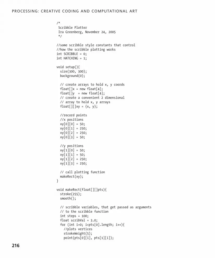
/*Scribble PlotterIra Greenberg, November 24, 2005*/
//some scribble style constants that control//how the scribble plotting worksint SCRIBBLE = 0;int HATCHING = 1;
void setup(){size(300, 300);background(0);
// create arrays to hold x, y coordsfloat[]x = new float[4];float[]y = new float[4];// create a convenient 2 dimensional// array to hold x, y arraysfloat[][]xy = {x, y};
//record points//x positionsxy[0][0] = 50;xy[0][1] = 250;xy[0][2] = 250;xy[0][3] = 50;
//y positionsxy[1][0] = 50;xy[1][1] = 50;xy[1][2] = 250;xy[1][3] = 250;
// call plotting functionmakeRect(xy);
}
void makeRect(float[][]pts){stroke(255);smooth();
// scribble variables, that get passed as arguments// to the scribble functionint steps = 100;float scribVal = 3.0;for (int i=0; i<pts[0].length; i++){//plots verticesstrokeWeight(5);point(pts[0][i], pts[1][i]);
PROCESSING: CREATIVE CODING AND COMPUTATIONAL ART
216
617xCH06.qxd 4/20/07 3:29 PM Page 216

LINES
217
6
//call scribble functionstrokeWeight(.5);if (i>0){scribble(pts[0][i], pts[1][i], pts[0][i-1], pts[1][i-1], !
steps, scribVal, SCRIBBLE);}if (i== pts[0].length-1){// show some hatching between last 2 pointsscribble(pts[0][i], pts[1][i], pts[0][0], pts[1][0], steps, !
scribVal*2, HATCHING);}
}}
/*scribble function plots lines between end points,determined by steps and scribVal arguments.2 styles are available: SCRIBBLE and HATCHING, whichare interestingly only dependent on parenthesesplacement in the line() function calls.*/void scribble(float x1, float y1, float x2, float y2, int steps, !
float scribVal, int style){
float xStep = (x2-x1)/steps;float yStep = (y2-y1)/steps;for (int i=0; i<steps; i++){if(style == SCRIBBLE){if (i<steps-1){line(x1, y1, x1+=xStep+random(-scribVal, scribVal), y1+= !
yStep+random(-scribVal, scribVal));}else {// extra line needed to attach line back to point- // not necessary in HATCHING styleline(x1, y1, x2, y2);
}}else if (style == HATCHING){
line(x1, y1, (x1+=xStep)+random(-scribVal, scribVal), !(y1+=yStep)+random(-scribVal, scribVal));
}}
}
617xCH06.qxd 4/20/07 3:29 PM Page 217

PROCESSING: CREATIVE CODING AND COMPUTATIONAL ART
218
Figure 6-34. Scribble Plotter sketch
There’s nothing new in this sketch. However, there are a few details that might need a littleclarification. The two constant variables SCRIBBLE and HATCHING have global scope since Ideclared them at the top of the program.
int SCRIBBLE = 0;int HATCHING = 1;
I passed them in as arguments from the makeRect() function to the scribble() function.They are capitalized, denoting that they are constants and should not be assigned a newvalue. If I really wanted to enforce that they shouldn’t be changed, I could have prefacedthe declaration statements with the word final, as in final int HATCHING = 1. final istechnically a Java keyword—it’s not within the Processing API—but it can be used withinProcessing. If you expand upon this sketch (which I hope you do), and want to add anotherscribble-style algorithm, then create a new constant, pass it as an argument, and detect forit in the scribble() function.
Hopefully you can make some sense of the scribble() function. I’m dividing up the x andy distances between the starting and ending points (passed into the function), and thenplotting lines to those intermediate positions. The random() function just jitters the place-ment of the line vertices. The SCRIBBLE style requires an extra line of code to ensure thatthe final line connects back to the original point. Try commenting out the line() functioncall within the else block inside the scribble function() conditional block.
617xCH06.qxd 4/20/07 3:29 PM Page 218

LINES
219
6
else {// extra line needed to attach line back to point- !
not necessary in HATCHING styleline(x1, y1, x2, y2); //try commenting this line out
}
The HATCHING style doesn’t require this fix. Finally, you’ll notice that I use the same variablename, steps, for the local variable in the makeRect() function and the parameter inthe scribble() function. I can do this because the steps variable is declared within themakeRect() function, not at the top of the sketch. Therefore, it is local in scope tothe makeRect() function and not visible anywhere else. Thus, I can use the same-namedvariable in both functions without any conflict. Of course, you can use unique names ifthat seems simpler to you. Personally, I find it hard to keep coming up with new relatednames, so I tend to reuse local variable names.
Well, enough of this low-level point recording business—let’s luxuriate through the rest ofthis chapter using Processing’s user-friendly vertex() function.
Applying the vertex functionThe vertex() function is called between the beginShape() and endShape() functions,which internally take care of the point recording and rendering just discussed. You’velooked at the POINTS mode already. The LINES mode works similarly, except instead ofrendering points, vertices are connected by lines in groups of two. For example, thefollowing code generates a horizontal line:
size(300, 300);background(255);beginShape(LINES);vertex(20, height/2);vertex(width-20, height/2);endShape();
Since the lines are laid down in groups of two vertices, adding a third vertex() functioncall will have no effect on the output:
size(300, 300);background(255);beginShape(LINES);vertex(20, height/2);vertex(width-20, height/2);vertex(width/2, height-20); //will have no effectendShape();
617xCH06.qxd 4/20/07 3:29 PM Page 219

I need a fourth vertex() call to generate another line:
size(300, 300);background(255);beginShape(LINES);vertex(20, height/2);vertex(width-20, height/2);vertex(width/2, height-20);vertex(width/2, 20);endShape();
This mode isn’t much of an improvement over just calling two line() functions. The fol-lowing code, for example, gives the exact same output as the last, but in four lines ratherthan eight:
size(300, 300);background(255);line(20, height/2, width-20, height/2);line(width/2, height-20, width/2, 20);
Creating line stripsThe situation, however, changes once you try to generate a line strip, which uses a no-argument version of beginShape(). By default, beginShape() creates an open and filledpath. You need to call noFill() if you want to generate an unfilled line strip. For example,the next sketch, shown in Figure 6-35, fills the display window with random vertices allconnected by a continuous path. If you used the line() function, you would need to keepfeeding previous second point positions into the next line call. I implemented thisapproach as a comparison, which I think you’ll agree is a much less elegant solution.
// elegant vertex() appraochsize(300, 300);background(255);strokeWeight(3);noFill();smooth();beginShape();for (int i=0; i<100; i++){vertex(random(width), random(height));
}endShape();
// kludgy line() approachsize(300, 300);background(255);strokeWeight(3);
PROCESSING: CREATIVE CODING AND COMPUTATIONAL ART
220
617xCH06.qxd 4/20/07 3:29 PM Page 220

LINES
221
6
smooth();float x = random(width);float y = random(height);for (int i=0; i<100; i++){float x2 = random(width);float y2 = random(height);line(x, y, x2, y2);x = x2;y = y2;
}
Figure 6-35. Line Strip sketch
Generating line strips opens up some interesting possibilities. One of these is mazecreation. Rather than considering maze structures as purely logic puzzles, which are alsovery interesting, I’m going to focus on the aesthetics of the geometric patterning of mazes.One fairly simple pattern is a concentric path, which begins at either an outer or innerboundary and proceeds to the opposite boundary with some predetermined rule pattern.For example, the rule might be to turn 90 degrees when you get within a certain distanceof an existing boundary.
617xCH06.qxd 4/20/07 3:29 PM Page 221

PROCESSING: CREATIVE CODING AND COMPUTATIONAL ART
222
The following sketch creates a concentric maze, but instead of using a more elegant rule-based algorithm, my cruder solution simply alters a vertical and horizontal stepping vari-able each iteration of the loop, beginning at the outer boundary. My implementation doesallow you to have asymmetry with regard to the x- and y-axes, as well as use any displaywindow size. I also utilize a few new functions in the loop that will require some clarifica-tion. Figure 6-36 shows the output of the code.
/*Concentric MazeIra Greenberg, November 25, 2005revised October 18, 2006*/
size(400, 400);background(0);strokeWeight(1);stroke(255);smooth();float x = width-1;float y = height-1;float y2 = 0, x2 = 0;float h = 0, w = 0;
//these values can be changedfloat wStep = 10.0;float hStep = 10.0;noFill();beginShape();vertex(x-w, y2+h);for (int i=min(width, height); i>min(width, height)/2; !
i-=max(wStep, hStep)){vertex(x-w, y-h);vertex(x2+w, y-h);vertex(x2+w, y2+h);w+=wStep;vertex(x-w, y2+h);h+=hStep;
}endShape();
617xCH06.qxd 4/20/07 3:29 PM Page 222

Figure 6-36. Concentric Maze sketch
Before I describe the new min() and max() functions I used in the sketch, I just want tomake sure you fully understand the following statements:
float x = width-1;float y = height-1;float y2 = 0, x2 = 0;float h = 0, w = 0;
In the first two lines, I subtract 1 from the width and height properties. I do this so that Ican see the maze output on the right and bottom edges of the display window. Try remov-ing the subtraction to see the difference. In the next two lines, I declare both the y2 andx2 variables as floats, and do the assignment on a single line. This is just a shortcut. Icould have done the assignment on two lines as well. I do the same thing on the next linewith the w and h variables. All four of these lines could also have been put on one line.
float y2 = 0, x2 = 0, h = 0, w = 0;
However, the benefit of only having to write “float” once is offset by the visual complexityof so many assignments. Ultimately, these type of issues are a matter of personal style.
L INES
223
6
617xCH06.qxd 4/20/07 3:29 PM Page 223

PROCESSING: CREATIVE CODING AND COMPUTATIONAL ART
224
The new function calls I used, min() and max(), are stuck in the head of the for loop:
for (int i=min(width, height); i>min(width, height)/2; i-=max(wStep,hStep)){...
The min() and max() functions each take two arguments and spit back the lower or highervalue, respectively. I used them to ensure that the maze was drawn correctly, regardless ofwhat the display window or wStep and hStep values were set to. The problem they solve iscorrecting for potential asymmetrical values assigned to the aforementioned variables. Forexample, if the width and height arguments in the size() function were set to 600 and400, my loop wouldn’t be able to adjust itself if I were using width to control the looplimit. I would always need the smaller dimension to be the loop limit for the auto-adjustment to work. Since (theoretically) users may sometimes make the width argumentbigger than height, or vice versa, there is no way to hard-code a value as the loop limit. Byusing the min() and max() functions, the loop automatically figures out the limiting vari-able (either the minimum value of either width or height, or the maximum value of wStepor hStep) and adjusts itself appropriately. This is a hard concept to explain in words, so Isuggest playing with the values for width, height, wStep, and hStep. You can also try sub-stituting the following for loop head into the sketch:
for (int i=width; i>width/2; i-=wStep)
while continuing to change all four values. You may notice that the substitute loop headcreates less ordered but more interesting output.
Next I created a tiled version of the maze (see Figure 6-37). The sketch puts together abunch of concepts discussed thus far in this chapter. There’s a lot more that could be donewith this sketch—for example, adding the scribble() function or additional random()functions. You could also add another maze pattern algorithm in the createMaze() func-tion. I’ve included comments that show you what variables you can safely change. (Ofcourse, safety aside, it‘s also helpful to sometimes break the code to get a better sense ofhow it works.)
/*Maze Tile 1Ira Greenberg, November 25, 2005revised October 18, 2006*/
// declare some varsfloat x, y, y2, x2, h, w, xShift, yShift;
//these values can be changedint xSclFactor = 3;int ySclFactor = 3;float wStep = 4;float hStep = 4;
617xCH06.qxd 4/20/07 3:29 PM Page 224

LINES
225
6
void setup(){//these values can be changedsize(400, 400);background(0);strokeWeight(1);stroke(255);noFill();smooth();//end changeable stuff
x = width/xSclFactor;y = height/ySclFactor;y2 = x2 = 0;for (int i=0; i<width; i+=x){for (int j=0; j<height; j+=y){h = w = 0;yShift = j;xShift = i;createMaze();
}}
}
void createMaze(){beginShape();vertex((x-w)+xShift, (y2+h)+yShift);for (float i=min(width/xSclFactor, height/ySclFactor); !
i>min(width/xSclFactor, height/ySclFactor)/2; !i-=max(wStep, hStep)){
vertex((x-w)+xShift, (y-h)+yShift);vertex((x2+w)+xShift, (y-h)+yShift);vertex((x2+w)+xShift, (y2+h)+yShift);w+=wStep;vertex((x-w)+xShift, (y2+h)+yShift);h+=hStep;
}endShape();
}
617xCH06.qxd 4/20/07 3:29 PM Page 225

Figure 6-37. Maze Tile 1 sketch
Line loopsIt’s also possible to close a line strip, turning it into a line loop. The endShape() functionhas an optional CLOSE argument that closes the strip. Since the CLOSE mode generatescomplete shapes, I thought it would be fun to generate some polygonal geometry; andthe best (and easiest) way to do that is to use a little trigonometry. Here’s a very simplesketch that generates a triangle (see Figure 6-38). (Yes, I know Processing comes with atriangle() function; but it’s actually a lot easier to use a little trig to calculate the verticesof a triangle rather than having to explicitly set the vertices. Also, once you have thetriangle code, you can easily modify it to generate any regular polygon—which I’ll showyou how to do shortly.)
PROCESSING: CREATIVE CODING AND COMPUTATIONAL ART
226
617xCH06.qxd 4/20/07 3:29 PM Page 226

LINES
227
6
//Create a Trianglesize(400, 400);background(0);stroke(255);strokeWeight(5);smooth();noFill();float x = 0, y = 0;// sets initial shape rotationfloat angle = 30;
beginShape();for (int i=0; i<3; i++){x = width/2+cos(radians(angle))*width/2.5;y = height/2+sin(radians(angle))*width/2.5;vertex(x, y);// create an equilateral tirangleangle+=120;
}endShape(CLOSE);
Figure 6-38. Create a Triangle sketch
Save for the two trig functions, the rest of this sketch should look pretty familiar. I thinkyou’ll also soon agree that implementing trig is relatively easy in Processing. The trianglecode relies on trig relationships, based on the unit circle, to do its thing. I discusstrigonometry briefly in Chapter 4, but also provide a more detailed explanation, includingan illustration of the unit circle, in Appendix B. Essentially, the unit circle tells you that thelocation of any point on a circle can be found by using an angle of rotation, commonly
617xCH06.qxd 4/20/07 3:29 PM Page 227

called theta, and the radius of the circle. However, the unit circle lives in a polar coordi-nate system, not the happy Cartesian system we use on a computer screen. Thus, you alsoneed to convert from the polar to the Cartesian coordinate system to get your x and ycoordinates. The two general statements to do all of this are as follows:
x coordinate = x position of the center of circle + cos(angle of rotation in radians) * radius
y coordinate = y position of the center of circle + sin(angle of rotation in radians) * radius
Returning to the two trig expressions in the triangle sketch, I used the center of the displaywindow as the center point of the unit circle, which will also be the center point of thetriangle. The function radians(angle) converts from degrees to radians; the actual con-version expression is (angle in radians) = (angle in degrees) * pi / 180, which is what theradians() function encapsulates. Lastly, I used width/2.5 as the radius.
Processing includes a function that lets you control how lines join together. Earlier, youlooked at the function strokeCap(), which controls the end caps of lines. The functionstrokeJoin() controls the way the end caps come together to form joints. There are threedifferent join options, in the form of integer arguments (constants): MITER, which is thedefault; BEVEL; and ROUND. This next example uses the triangle code to show the differencein the respective join options (see Figure 6-39 for the output).
//create 3 trianglessize(600, 200);background(0);stroke(255);noFill();strokeWeight(10);smooth();float x = 0, y = 0;// sets initial shape rotationfloat angle = 30;// join typesint[]joins = {MITER, BEVEL, ROUND};for (int j=1; j<4; j++){beginShape();strokeJoin(joins[j-1]);for (int i=0; i<3; i++){x = (width/4)*j+cos(radians(angle))*width/8;y = height/2+sin(radians(angle))*width/8;vertex(x, y);// create an equilateral tirangleangle+=120;
}endShape(CLOSE);
}
PROCESSING: CREATIVE CODING AND COMPUTATIONAL ART
228
617xCH06.qxd 4/20/07 3:29 PM Page 228

LINES
229
6
Figure 6-39. Create 3 Triangles sketch
Polygons and patternsNow that you have a basic understanding about how the trig functions can be used toidentify a point on a circle, you can exploit that knowledge to generate any regular poly-gon. (Even if you don’t yet fully grasp—or even care—how the trig functions work, youcan still use them. In fact, through using them, you’ll get a better understanding of howthey work than through reading about them). The following example incorporates thebeginShape() and endShape(CLOSE) functions in a basic polygon-creation algorithm (theoutput is shown in Figure 6-40):
/*Poly MakerIra Greenberg, November 26, 2005revised October 18, 2006*/
void setup(){size(400, 400);background(0);smooth();noFill();makePoly(width/2, height/2, 9, 150, 255, 8, MITER);
}
void makePoly(int x, int y, int points, float radius, !int strokeCol, float strokeWt, int strokeJn){float px=0, py=0;float angle = 0;stroke(strokeCol);strokeJoin(strokeJn);strokeWeight(strokeWt);beginShape();
617xCH06.qxd 4/20/07 3:29 PM Page 229

PROCESSING: CREATIVE CODING AND COMPUTATIONAL ART
230
for (int i=0; i<points; i++){px = x+cos(radians(angle))*radius;py = y+sin(radians(angle))*radius;vertex(px, py);angle+=360/points;
}endShape(CLOSE);
}
Figure 6-40. Poly Maker sketch
Try changing some of the argument values in the function call makePoly(width/2,height/2, 9, 150, 255, 8, MITER);. You can now use the makePoly() function to dosome interesting things. Overlapping geometry can lead to fascinating patterns. This wasone of the first experiments I did when I was learning to program that got me reallyexcited about the aesthetic potential of code.
The last three sketches in the chapter generate geometric patterns. I’ve included twoscreen shots for each sketch. The first sketch, shown in Figures 6-41 and 6-42, is apolygonal table structure, with a bunch of random() functions thrown in. The second,shown in Figures 6-43 and 6-44, is a spiral built of polygons; and the third, shown inFigures 6-45 and 6-46, is a polystar constructed of overlapping radial geometry. This lastexample utilizes a modified polygon function that creates both regular polygons and poly-stars. A “polystar,” which is my own made-up name, is just a polygon with a second radius,like a star. These two radii can also have both negative and positive values. As always, thereare numerous values to change in all three of these sketches, with a wide range of poten-tial output. These examples incorporate much of the stuff covered in this chapter, so I’dtake some time with them before heading to Chapter 7. Also try not to worry if some/mostof the code still looks like gobbledygook. You’ll be revisiting all the coding concepts in thischapter throughout the rest of the book.
617xCH06.qxd 4/20/07 3:29 PM Page 230

Poly Pattern I (table structure)/*Poly Pattern IIra Greenberg, November 26, 2005revised October 18, 2006pattern: table structure*/void setup(){size(400, 400);background(0);smooth();
//you can change these valuesint hGap = 12;int wGap = 12;int[]rads = { 3, 4, 5, 6, 7, 8 };int randSize = 3;int randPos = 3;
for (int j=0; j<=width; j+=wGap){for (int i=0, radCntr=0; i<=height; i+=hGap, radCntr++){makePoly(j+random(-randPos, randPos), i+randPos, rads[radCntr],!
wGap/2+random(-randSize, randSize), 255, radCntr*.4, MITER);
// reset counter to avoid ArrayIndexOutOfBounds errorif (radCntr>rads.length-2){radCntr = 0;
}}
}}
void makePoly(float x, float y, int points, float radius, !int strokeCol, float strokeWt, int strokeJn){
float px=0, py=0;float angle = 0;stroke(strokeCol);noFill();strokeJoin(strokeJn);strokeWeight(strokeWt);beginShape();for (int i=0; i<points; i++){px = x+cos(radians(angle))*radius;py = y+sin(radians(angle))*radius;vertex(px, py);angle+=360/points;
}endShape(CLOSE);
}
LINES
231
6
617xCH06.qxd 4/20/07 3:29 PM Page 231

PROCESSING: CREATIVE CODING AND COMPUTATIONAL ART
232
Figure 6-41. Poly Pattern I (table structure) sketch, variation 1
Figure 6-42. Poly Pattern I (table structure) sketch, variation 2
617xCH06.qxd 4/20/07 3:29 PM Page 232

Poly Pattern II (spiral)/*Poly Pattern IIIra Greenberg, November 26, 2005revised October 18, 2006pattern: spiral*/
void setup(){size(400, 400);background(0);smooth();float radius = 0, radius2 = 0;float x = 0, y = 0;float ang = 0;while(x<width*1.5){y = height/2+sin(radians(ang))*radius;x = width/2+cos(radians(ang))*radius;makePoly(x, y, 8, radius2, int(radius2*30), 6, BEVEL);
// you can change these valuesang+=1.1;radius+=.059;radius2+=.0016;
}}
void makePoly(float x, float y, int points, float radius, !int strokeCol, float strokeWt, int strokeJn){
float px=0, py=0;float angle = 0;stroke(strokeCol);noFill();strokeJoin(strokeJn);strokeWeight(strokeWt);beginShape();for (int i=0; i<points; i++){px = x+cos(radians(angle))*radius;py = y+sin(radians(angle))*radius;vertex(px, py);angle+=360/points;
}endShape(CLOSE);
}
LINES
233
6
617xCH06.qxd 4/20/07 3:29 PM Page 233

Figure 6-43. Poly Pattern II (spiral) sketch, variation 1
Figure 6-44. Poly Pattern II (spiral) sketch, variation 2
PROCESSING: CREATIVE CODING AND COMPUTATIONAL ART
234
617xCH06.qxd 4/20/07 3:29 PM Page 234

LINES
235
6
Poly Pattern III (polystar)/*Poly Pattern IIIIra Greenberg, November 26, 2005revised October 18, 2006Pattern: PolyStar*/
void setup(){size(400, 400);background(random(255));smooth();float ang = 0;int steps = int(random(30, 200));for (int i=0; i<steps; i++){makePolyStar(width/2, height/2, int(random(3, 10)), !
ang+=360/steps, random(-width/2, width/2), !random(-width/2, width/2), int(random(255)), !random(.25, 5), MITER);
}}
void makePolyStar(float x, float y, int points, float initAngle, !float radius, float radius2, int strokeCol, float strokeWt, !int strokeJn){
float px=0, py=0;float angle = initAngle;float initRadius = radius;float halfRadius = radius2;stroke(strokeCol);noFill();strokeJoin(strokeJn);strokeWeight(strokeWt);beginShape();// if 2nd radius create polystar// else create regular polyif (radius2 !=0){points*=2;
}for (int i=0; i<points; i++){//alternates radius length if polystarif (radius2 != 0 && i%2 == 0){radius = halfRadius;
}else {radius = initRadius;
}px = x+cos(radians(angle))*radius;
617xCH06.qxd 4/20/07 3:29 PM Page 235

236
PROCESSING: CREATIVE CODING AND COMPUTATIONAL ART
py = y+sin(radians(angle))*radius;vertex(px, py);angle+=360/points;
}endShape(CLOSE);
}
Figure 6-45. Poly Pattern III (polystar) sketch, variation 1
617xCH06.qxd 4/20/07 3:29 PM Page 236

6
237
LINES
Figure 6-46. Poly Pattern III (polystar) sketch, variation 2
SummaryThe beginning of this chapter let you look a little under Processing’s hood, and it discussedhow Processing functions are internally implemented. Once you got past this section, youdove into Processing’s point() and line() functions, and generated a couple of interest-ing linear outputs. This chapter utilized lots of randomization in the sketches, demonstrat-ing the power of controlled chaos as a creative coding force. You began with some simple,unstructured sketches that executed one line at a time, and continued on to more com-plex sketches that utilized modular structures, such as Processing’s setup() function, aswell as some custom functions and nested loops.
617xCH06.qxd 4/20/07 3:29 PM Page 237

You worked with a number of Processing’s functions in this chapter, including point(),line(), vertex(), beginShape(), and endShape(). You also looked briefly at PImage,which you’ll return to again in later chapters. Using the vertex() function, you createdsome fairly complex table structures and maze patterns, and even tackled a littletrigonometry with the polygonal sketches.
A lot has been covered in this chapter, and I’d say you have earned a little brain downtime.The next chapter will look at curves, which will include a review of a lot of the conceptscovered in this chapter. Of course, there will also be a fair amount of new (and I thinkcool) stuff. I recommend, after your earned downtime, reviewing some of the sketchescovered in this chapter before moving on. I also think it might be a good time to refer tothe reference material in the earlier chapters (as well as the language reference inAppendix A) on some of the more irksome concepts you might still be fuzzy on. Of course,moderation aside, if you’re feeling up to it, just turn the page and dive into the joy ofcurves.
PROCESSING: CREATIVE CODING AND COMPUTATIONAL ART
238
617xCH06.qxd 4/20/07 3:29 PM Page 238

617xCH06.qxd 4/20/07 3:29 PM Page 239

617xCH07.qxd 4/17/07 1:38 PM Page 240

7 CURVES
617xCH07.qxd 4/17/07 1:38 PM Page 241

Curvy stuff is difficult for people to understand. Had I taken a calculus class earlier in mylife, this fact would have been blatantly obvious. When drawing directly from a model,edges are indistinct and there are all sorts of subtle foreshortening. In time, you learn howto, in a sense, “not draw” what’s not there, which is often the secret to allowing the curvestructures to emerge in the drawing. When it comes to coding, curves again prove espe-cially challenging, and often require a more “mathy” approach than when working withlines. Processing does makes it relatively easy to generate simple curves, but being able toprecisely control a combination of curves to create a form such as a human figure is verydifficult.
That being said, the additional effort and added complexity of dealing with curves is wellworth it, as there is something exciting about seeing organic forms and animation emerge;it’s what really got me hooked on coding to begin with. In my classes, at the beginning ofa semester I’ll often show organic code-based animation examples to my students; thisalways gets them oohing and ahhing. (Of course, they make other sounds when they beginwrestling with the actual curve implementation and math.)
This chapter will explore curves in detail, beginning with how to make the transitionbetween straight lines and curves. After that, I’ll discuss creating curves using trig andpolynomials, and then I’ll explain Processing’s curve functions in depth.
Making the transition from lines to curvesI began the last chapter with a discussion about points, and showed how a line is really justa continuous path of points. I eventually showed you how to utilize a more efficient systemof terminal vertices to describe the beginning and ending points of lines. Processing’s
line() function takes four arguments (the x and y components of twopoints) and joins the points with a straight line. In beginning to thinkabout curves, you need to consider how Processing connects the twopoints with a line, which you can then modify into a curve. As a review,here is a simple script to generate a vertical line utilizing a series ofpoints, as shown in Figure 7-1:
size(200, 200);background(255);int margin = height/15;strokeWeight(5);for (int i=margin; i<height-margin; i++){point(width/2, i);
}
Hopefully this looks very familiar. The for loop generates a vertical line in the middle ofthe display window from a series of points, beginning at margin and ending at height(of the display window) minus margin. You’ll remember that point() is really a call to theline() function, using the same two points as arguments; that’s why I was able to changethe thickness of the points, and thus the line, with strokeWeight(5). As an example, here’sthe same sketch using line():
PROCESSING: CREATIVE CODING AND COMPUTATIONAL ART
242
Figure 7-1.Combining points
into a line
617xCH07.qxd 4/17/07 1:38 PM Page 242

size(200, 200);background(255);int margin = height/15;strokeWeight(5);for (int i=margin; i<height-margin; i++){line(width/2, i, width/2, i); // notice both points are the same
}
In this simple sketch, it can be said in describing the line that the x position of the lineremains constant while the y position changes. You may remember that the slope of aline is the change in y divided by the change in x. If you tried to figure out the slope of thevertical line, you would use the following expression:
y2-y1/x2-x1
= ((height-margin)-margin)/(width/2-width/2)= 174/0 // oops, can't divide by 0slope = undefined
You see the problem with this expression—you can’t divide by 0. Therefore, a vertical linehas no slope, or the slope is undefined. How about a horizontal line? Following is thesketch modified to make a horizontal line:
size(200, 200);background(255);int margin = width/15;strokeWeight(5);for (int i=margin; i<width-margin; i++){line(i, height/2, i, height/2); // both points are the same
}
Calculating the slope of this line results in the following:
= (height/2-height/2)/((width-margin)-margin)= 0/174slope = 0
Confusingly, a horizontal line has a slope of 0. This is the kind of annoying detail that con-tributes to many cases of “math coma.” We’re not going to focus on vertical and horizon-tal lines (which aren’t terribly exciting). Instead, I’ll start with diagonals, which will lead tocurves—which are actually very interesting (honestly).
The equation for the vertical line was x = height/2, and the equation for the horizontal linewas y = width/2. You don’t need to really worry so much about equations, but it’s helpfulto understand a little about what’s happening to the x and y values when plotting differenttypes of lines and curves. You’ll notice in both the vertical and horizontal line equationsthat only one value (x or y) is needed to describe the line. That’s because only one ofthe values is changing; the other remains constant as the line is plotted. To describe a diag-onal line, both of the x and y values need to change as the line is plotted. There are acouple ways to express a line, but I think the simplest is using the slope-intercept form:
CURVES
243
7
617xCH07.qxd 4/17/07 1:38 PM Page 243

y = mx + b. y and x are just the coordinate values, m is the slope, and b is the place on they-axis that the line intercepts. Again, you don’t need to explicitly use the classical equa-tions, but knowing them can help you better understand what’s happening in your sketch.
Here’s a diagonal line example (shown in Figure 7-2):
/*Diagonal Line IIra Greenberg, December 3, 2005*/size(200, 200);background(255);int margin = width/15;strokeWeight(5);smooth();float x = margin, y = margin;float deltaX = 1.2;float deltaY = 1.2;
if (deltaX>deltaY){while(x<width-margin){point(x, y);x += deltaX;y += deltaY;
}} else{while(y<height-margin){point(x, y);x += deltaX;y += deltaY;
}}
Figure 7-2. Combining points into a diagonal
PROCESSING: CREATIVE CODING AND COMPUTATIONAL ART
244
617xCH07.qxd 4/17/07 1:38 PM Page 244

You should notice some familiar structures in this example. I called the smooth() functionto turn on anti-aliasing, and I used two while loops nested within a conditional if...elsestructure to ensure that the line stays in the display window. Try changing the values of thedeltaX and deltaY variables to see how the diagonal changes (see Figures 7-3 and 7-4 fora couple of examples).
deltaX = .7;deltaY = 1.2;
Figure 7-3. A more vertical diagonal
deltaX = 1.4;deltaY = .2;
Figure 7-4. A more horizontal diagonal
CURVES
245
7
617xCH07.qxd 4/17/07 1:38 PM Page 245

As the deltaX and deltaY values become farther apart, the line visually approaches eithera vertical or horizontal line. The most diagonal line (if there is such a thing) is when deltaXand deltaY are equal, or the change in x and the change in y are equal. As you might haveguessed, this is also when the slope is 1. Slope is a very important property in describingmotion, which I’ll cover in Chapter 11. Speed is the rate at which position is changing.When you plot a diagonal line as a function of distance and time, as shown in Figure 7-5,the slope of the plotted line is speed.
Figure 7-5. Speed plot
Creating your first curveWithout acceleration, speed is a constant and will always generate a straight line, as therate of change will be constant. Starting with different constant values of speed, you canchange the steepness, or slope, of the line, as the previous example showed, but you cannever get a curve if you keep the speed (or slope) constant. Thus, it would seem logical, ifyou wanted to generate a curve, to use a changing speed value—which is precisely whatyou’ll do next. This is also the reason why curves, with regard to motion, describe acceler-ation, or the change in speed. This next sketch (shown in Figure 7-6) is a curve plot:
/*Curve IIra Greenberg, December 3, 2005*/size(200, 200);background(255);
PROCESSING: CREATIVE CODING AND COMPUTATIONAL ART
246
617xCH07.qxd 4/17/07 1:38 PM Page 246

int margin = height/15;strokeWeight(5);smooth();float x = margin, y = margin;float xSpeed = 1.1, ySpeed = 1.02;while(y<height-margin){point(x, y);x+=xSpeed; // arithmetic progressiony*=ySpeed; // geometric progression
}
Figure 7-6. Simple curve created from points
Congratulations, you just plotted your first curve! There are many ways to implement acurve plot. I used a simple approach that increments x by xSpeed (using addition):
x+=xSpeed; // arithmetic progression
and y by ySpeed (using multiplication).
y*=ySpeed; // geometric progression
Notice that the initial values I assigned to the two speed variables are very different. In thewhile loop, x is incremented by xSpeed in a similar fashion to how x was incremented bydeltaX in the diagonal example. x increases by 1.1 each iteration of the loop. This typeof progression, generated by adding a constant value (in this case 1.1) is called anarithmetical progression. Here are the first and last three values of the progression, wherethe initial values of x and y are both 13 (margin value):
CURVES
247
7
617xCH07.qxd 4/17/07 1:38 PM Page 247

First three values: 14.1, 15.2, 16.3
Last three values: 159.3, 160.4, 161.5
As you can see, the change between any two consecutive values will always be xSpeed(1.1). In contrast, y is incremented by the constant 1.02 using multiplication. This is calleda geometric progression. Here are the first and last three values in this progression:
First three values: 13.26, 13.53, 13.80
Last three values: 181.04, 184.66, 188.35
The difference between any consecutive values will no longer be a constant value through-out the entire progression. This change in speed generates a curve. Let’s alter some valuesin the curve plot to see how it effects the curve (see Figures 7-7 and 7-8):
float xSpeed = .5, ySpeed = 1.02;
Figure 7-7. Faster falling curve
float xSpeed = 6.6, ySpeed = 1.11;
PROCESSING: CREATIVE CODING AND COMPUTATIONAL ART
248
617xCH07.qxd 4/17/07 1:38 PM Page 248

Figure 7-8. Revealing the points making up the curve
In Figure 7-7, I just decreased xSpeed, making the curve fall faster, since the x progressionis slower. In the second example, I increased both variables considerably, maintaining asimilarly shaped curve, but with a much faster overall progression, revealing the pointsmaking up the curve.
I want to look at some other relatively simple ways to generate curves; but before I do,here are some more interesting examples building upon what you just learned(see Figure 7-9). (If you don’t see any output in the examples, try raising thestrokeWeight(1.5) argument from 1.5 to 2 or above).
/*Curves IIra Greenberg, December 4, 2005*/int steps = 300;float[]x = new float[steps];float[]y = new float[steps];float[]xSpeed = new float[steps];float[]ySpeed = new float[steps];
void setup(){size(400, 400);background(255);float margin = height*.1;smooth();strokeWeight(1.5);
CURVES
249
7
617xCH07.qxd 4/17/07 1:38 PM Page 249

for (int i=0; i<steps; i++){x[i] = 0;y[i] = random(margin);xSpeed[i] = random(.75, 1.2);ySpeed[i] = random(1.0075, 1.04);
}
for (int i=0; i<steps; i++){while(y[i]<height){point(x[i], y[i]);x[i]+=xSpeed[i];y[i]*=ySpeed[i];
}}
}
Figure 7-9. Falling random strands
This example uses arrays to generate 300 curves, with some random values. The overlap-ping curves generate interesting forms, suggestive of flowing strands of hair or water. Asthe points begin spacing out, a system of particles begins emerging. You can exploit thisphenomenon further by adding a minimal amount of collision detection, allowing the par-ticles to deflect off the display window edges. The next example, shown in Figure 7-10, isimplemented a little differently and includes window edge detection.
PROCESSING: CREATIVE CODING AND COMPUTATIONAL ART
250
617xCH07.qxd 4/17/07 1:38 PM Page 250

/*Curves IIIra Greenberg, December 4, 2005*/int particles = 25;float[]x = new float[particles];float[]y = new float[particles];float[]xSpeed = new float[particles];float[]ySpeed = new float[particles];float[]accel = new float[particles];float gravity = .75;
void setup(){size(800, 400);background(0);smooth();strokeWeight(1.5);stroke(255);
//fill speed arrays with initial valuesfor (int i=0; i<particles; i++){xSpeed[i] = random(.75, 1.2);accel[i] = random(.005, .2);
}
for (int i=0; i<particles; i++){//stop particle on collision with right edge of display windowwhile(x[i]<width){x[i]+=xSpeed[i];
// double assignment creates y accelerationySpeed[i] += accel[i];y[i]+=ySpeed[i];point(x[i], y[i]);
// check ground detection onlyif ( y[i]>=height){// reverse particle directionySpeed[i]*=-1;// lower particle speedySpeed [i]*=gravity;// keep particle from sliding out of windowy[i]=height;
}}
}}
CURVES
251
7
617xCH07.qxd 4/17/07 1:38 PM Page 251

Figure 7-10. Falling random bouncing strands
This example is similar to the last, but I achieved the curved motion using a slightly differ-ent algorithm. Instead of multiplying y by a ratio, I used a double arithmetic incrementa-tion. The lines
ySpeed[i] += accel[i];y[i] += ySpeed[i];
create the acceleration. It may not be immediately apparent how this works. However, ifyou look at a few values during the loop iterations, it becomes clear what’s happening. Tokeep things simple, let’s assume the value assigned to accel, for one of the particles, is .1.Following are the ySpeed and y values after five iterations:
iteration1: ySpeed= .1, y = .1iteration2: ySpeed = .2, y = .3 (y change: .2)iteration3: ySpeed = .3, y = .6 (y change: .3)iteration4: ySpeed = .4, y = 1.0 (y change: .4)iteration4: ySpeed = .5, y = 1.5 (y change: .5)
Notice how the y value is changing by an increasing interval: .2, .3, .4, .5; this is what gen-erates the acceleration.
The display window collision detection allows the particles to remain active longer andthus graphically add to the image. The detection is pretty straightforward: if a particle’s yposition is greater than or equal to the height of the display window, then reverse thedirection of the particle and also multiply ySpeed by the gravity variable. Here’s the codesnippet:
// check ground detection onlyif ( y[i]>=height){// reverse particle directionySpeed[i]*=-1;
PROCESSING: CREATIVE CODING AND COMPUTATIONAL ART
252
617xCH07.qxd 4/17/07 1:38 PM Page 252

// lower particle speedySpeed[i]*=gravity;// keep particle from sliding out of windowy[i]=height;
}
This expression slowly reduces the particle’s velocity (ySpeed) until it is very near zero.However, because ySpeed will actually never reach zero, I am forced to add the finalassignment, y[i]=height, which keeps the particles from slowly creeping off the bottomof the screen. I’ll revisit this issue again in more detail in Chapter 11. As always, play withthe code. If you comment out this last assignment, you should notice the output is a littlelower in relation to the display window.
In the next example (shown in Figure 7-11), I pushed this particle effect a little further,utilizing a new material property, more randomization, and additional display edge detec-tion. There’s nothing really new in the example, but it should reveal some more of theinteresting effects you can get coding curved motion. This example can take a long time torender—up to 30 seconds. Decreasing the strokeWtMin and strokeWtMax argument valueswill speed things up. However, on some systems, too small a value may make the curvesundetectable.
/*Curves IIIIra Greenberg, December 4, 2005// this takes some time to render*/
// changeable variablesint particles = 125;int timeLimit = 2000;float particleSpan = 2;float accelMin = .005;float accelMax = .2;float strokeWtMin = 1.25;float strokeWtMax = 1.6;float materialMin = .25;float materialMax = .99;float gravity = .9;
// not meant to be changedint timer;float[]x = new float[particles];float[]y = new float[particles];float[]xSpeed = new float[particles];float[]ySpeed = new float[particles];float[]accel = new float[particles];float[]material = new float[particles];float[]strokeWts = new float[particles];
CURVES
253
7
617xCH07.qxd 4/17/07 1:38 PM Page 253

void setup(){size(800, 400);background(0);smooth();stroke(255);
//fill speed arrays with initial valuesfor (int i=0; i<particles; i++){x[i] = random(width/2-10, width/2+10);xSpeed[i] = random(-particleSpan, particleSpan);accel[i] = random(accelMin, accelMax);material[i] = random(materialMin, materialMax);strokeWts[i] = random(strokeWtMin, strokeWtMax);
}
for (int i=0; i<particles; i++){//timer controls while looptimer = 0;strokeWeight(strokeWts[i]);
while(timer++ < timeLimit){x[i]+=xSpeed[i];// double assignment creates y accelerationySpeed[i]+=accel[i];y[i]+=ySpeed[i];point(x[i], y[i]);
// check ground detectionif ( y[i]>=height){// reverse particle directionySpeed[i]*=-1*material[i];// lower particle speedySpeed[i]*=gravity;// keep particle from sliding out of windowy[i]=height;
}// check wall detectionif ( x[i]>=width || x[i]<0){// reverse particle horizontal directionxSpeed[i]*=-1;
}}
}}
PROCESSING: CREATIVE CODING AND COMPUTATIONAL ART
254
617xCH07.qxd 4/17/07 1:38 PM Page 254

Figure 7-11. Curves simulating a fountain
Creating curves using trigAnother relatively easy way to generate a curve is to utilize a trig function. Sine and cosinefunctions both generate a repeating periodic wave. Here’s a simple example (shown inFigure 7-12):
//trig wavesize(400, 200);background(0);stroke(255);float angle = 0;float amplitude = 10;float x = 0, y = 0;float xSpeed = 1;float frequency = 3.0;smooth();
for (int i=0; i<width; i+=xSpeed){strokeWeight(30);x+= xSpeed;//siny = height/3 + sin(radians(angle))*amplitude;point(x, y);//cosiney = 2*(height/3) + cos(radians(angle))*amplitude;point(x, y);angle+=frequency;
}
CURVES
255
7
617xCH07.qxd 4/17/07 1:38 PM Page 255

Figure 7-12. Creating simple curves with trigonometry
The sin() and cos() functions are controlled by the incrementation of the angle (fre-quency) and the value of the amplitude. Try changing these variables to see how the plotsare affected. You can also use a damping variable (which acts like gravity in the particleexample) to decrease the amplitude of the trig functions over time. Here’s an example ofthis (see Figure 7-13):
//waves with dampingsize(400, 200);background(0);stroke(255);float angle = 0;float amplitude = 30;float x = 0, y = 0;float xSpeed = 1;float frequency = 6.0;float damping = .994;strokeWeight(3);smooth();
for (int i=0; i<width; i+=xSpeed){x+=xSpeed;//siny = height/3 + sin(radians(angle))*amplitude;point(x, y);//cosiney = 2*(height/3) + cos(radians(angle))*amplitude;point(x, y);amplitude*=damping;angle+=frequency;
}
PROCESSING: CREATIVE CODING AND COMPUTATIONAL ART
256
617xCH07.qxd 4/17/07 1:38 PM Page 256

Figure 7-13. Damping effect on curves
In the last chapter, I demonstrated a scribble function, where endpoints of a line were sentto a function that randomly jittered points between the terminal points, creating a moreorganic-looking line. You can use trig functions in a similar capacity. I thought it might beinteresting to put the particle effect together with the trig function to create particlewaves (see Figure 7-14); it will also be a good review of using custom functions.
This is a fairly complex sketch. Each part of it is encapsulated in a function, and there areno global variables. Thus, the individual functions speak to each other through functioncalls. I recommend playing with the sketch for a while before reviewing the code. I com-pletely parameterized the main particle function, so it’s easy to mess with the variablesin the setup() structure—seeing how the changes affect the output, as illustrated inFigure 7-15—before diving into the code guts.
/*Particle WaveIra Greenberg, December 5, 2005revised January 26, 2007*/
void setup(){size(800, 400);background(0);smooth();
/*lots of stuff to manipulate. I packedthe arguments into arrays just to make thesetParticles function argument/parameterlists less unwieldy*///particle style/* increase strokeWt ifyou don't see any output*/float strokeWt = 1.5;float strokeCol= 255;float[]strokeStyle = { strokeWt, strokeCol };
CURVES
257
7
617xCH07.qxd 4/17/07 1:38 PM Page 257

//particle limitsint timeLimit = 1000;int particleCount = 100;int[]particleLimits = { timeLimit, particleCount };
//particle dynamicsfloat amplitudeMin = .5;float amplitudeMax = 4.0;float frequencyMin = 4.0;float frequencyMax = 40.0;float materialMin = .25; // leadfloat materialMax = .99; // rubberfloat[]particleDynamics = { amplitudeMin, amplitudeMax, !frequencyMin, frequencyMax, materialMin, materialMax};
// speed limitsfloat accelMin = .005;float accelMax = .2;float xSpeedMin = -2.0;float xSpeedMax = 2.0;float[]speedLimits = { xSpeedMin, xSpeedMax, !accelMin, accelMax };
float gravity = .85;//position of particle emitterfloat emitterX = width/2;float emitterY = 0;float[]world = { gravity, emitterX, emitterY };
//start particle enginesetParticles(strokeStyle, particleLimits, !particleDynamics, speedLimits, world);
}
// main particle engine - fully parameterizedvoid setParticles(float[]strokeStyle, int[]particleLimits, float[]particleDynamics, float[]speedLimits, float[]world){//create arraysfloat[]xSpeed = new float[particleLimits[1]];float[]ySpeed = new float[particleLimits[1]];float[]accel = new float[particleLimits[1]];float[]x = new float[particleLimits[1]];float[]y = new float[particleLimits[1]];float[]amplitude = new float[particleLimits[1]];float[]frequency = new float[particleLimits[1]];float[]material = new float[particleLimits[1]];
PROCESSING: CREATIVE CODING AND COMPUTATIONAL ART
258
617xCH07.qxd 4/17/07 1:38 PM Page 258

// particle stylestrokeWeight(strokeStyle[0]);stroke(strokeStyle[1]);
//angle used as argument for makeWaves function callfloat angle = 0;
//fill arraysfor (int i=0; i<particleLimits[1]; i++){xSpeed[i] = random(speedLimits[0], speedLimits[1]);accel[i] = random(speedLimits[2], speedLimits[3]);amplitude[i] = random(particleDynamics[0], particleDynamics[1]);frequency[i] = random(particleDynamics[2], particleDynamics[3]);material[i] = random(particleDynamics[4], particleDynamics[5]);//emitter initial positionx[i] = world[1];y[i] = world[2];
}
// dynamics enginefor (int i=0; i<particleLimits[1]; i++){for (int j=0; j<particleLimits[0]; j++){x[i]+=xSpeed[i];// add waviness to call to makeWaves functionx[i]=makeWaves(x[i], angle+=frequency[i], amplitude[i]);ySpeed[i]+=accel[i];y[i]+=ySpeed[i];// plot function just calls point() methodplot(new float[]{ x[i], y[i] }
);
//ground detectionif (y[i]>=height){ySpeed[i]*=-1*material[i];ySpeed[i]*=world[0];y[i] = height;
}//wall detectionif (x[i]>=width || x[i]<=0){xSpeed[i] *=-1;
}}
}}
CURVES
259
7
617xCH07.qxd 4/17/07 1:38 PM Page 259

//generate wavefloat makeWaves(float x, float angle, float amplitude){x+=sin(radians(angle))*amplitude;return x;
}
// draw pointsvoid plot(float[]pt){point(pt[0], pt[1]);
}
Figure 7-14. Curves as particle waves, example 1
Figure 7-15. Curves as particle waves, example 2
PROCESSING: CREATIVE CODING AND COMPUTATIONAL ART
260
617xCH07.qxd 4/17/07 1:38 PM Page 260

By using functions to organize a program, you get the benefit of modularity, but also theburden of added abstraction. It doesn’t help that so many of the parameters are indexpositions in arrays. However, with a sketch this complex, you need ways of cutting downon the variable clutter. Another, and better, way to code this sketch would be using anobject-oriented approach. This would allow for even greater modularity and potentialcode reuse. For example, I could create a class for each of the main elements in thesketch: Particle, Emitter, Dynamics, Wave, World, and so forth. This would allow me toreally encapsulate the functionality of each of these constructs. I would also design therelationships between these different classes. Of course, this approach also brings lots ofadded abstraction to the process, so it’s not the best approach for new coders. Later in thebook, when you’re an old, salty hackster, I’ll approach some problems using object-oriented programming (OOP). Before moving on, though, I want go over a few elements inthe last particle wave example.
I avoided global variables and declared local variables within the functions. This encour-ages code reuse, as each function is a self-contained processing unit. To use the function,you just need to know the parameter list, or the interface to the function. The parameterlist shows the input that the function requires to do its thing. The return type of the func-tion shows what value, if any, the function returns when it is called. For example, the floatmakeWaves() function returns a float value every time it’s called. Returning a value shouldnot be confused with outputting something to the display window. The plot() function,for example, outputs points to the screen, but the function doesn’t return any value whenit is called. Another benefit of using all local variables defined within functions is that thereis no danger of name collisions. I can use the same named variables in each function with-out any ambiguity because each variable has local scope. If I need the value of a variableoutside the function, I need to pass it as an argument, as I do throughout the program.
I used a bunch of convenience arrays in the setup() function. I use the term “conven-ience” because I could have just passed the variables individually as arguments to thesetParticles() function. However, the parameter list, defined in the head of thesetParticles() function, would have needed to account for all these variables, includingtheir type. This list would have included 17 parameters. Instead, by packaging the variablesinto logical arrays, I only needed to pass five arguments to the setParticles() function(which of course needed five parameters of the same type declared in the head ofthe function). The burden of this organizational abstraction is that once in thesetParticles() function, I needed to, as the function designer, carefully decode whatvalue each array index contained. However, since all the values required by the functionare passed in as arguments, once completed, I theoretically never have to mess with theinsides of this function again. If I want to change the output of the function, I simplychange the values I pass to it—it’s a black box construction.
One issue in this example that may be confusing to new coders is my use of function callswithin other functions, especially with regard to using a returned value in an assignment.For example, from within the setParticles() function, I call the makeWaves() function:
// called from within the setParticles() functionx[i]=makeWaves(x[i], angle+=frequency[i], amplitude[i]);
Try not to get confused by all the array notation (all the [i]s) in the function. Everythingis efficiently getting processed in a for loop, and each of the variables is a primitive array;
CURVES
261
7
617xCH07.qxd 4/17/07 1:38 PM Page 261

the loop incrementally moves through each index of the array, processing all the data.However, in any single iteration of the loop, only one value in each of the arrays is beingprocessed/used at a time. So, for example, the second iteration of the for loop i is equalto 1, and therefore the second value in each of the arrays is the one being processed/used.You should also notice that I am using x[i] as both the variable receiving the assignmentand the first argument in the makeWaves() function call. I remember being really confusedwhen I first came across this sort of thing—it didn’t seem to make sense. To understandwhat’s happening, you need to consider the order in which things take place. Assignmentoperations happen from right to left. Thus, the function will do its thing before the assign-ment takes place. Since the makeWaves() function returns a float value, the returned valueis assigned to x[i] after the function finishes. I am just using the makeWaves() function toincrement the x[i] value by the trig function. The second argument, angle+=frequency[i], increments the angle variable each iteration of the loop by the currentvalue of frequency[i]. The increasing angle value is needed by the makeWaves() functionto keep its internal trig function moving. The last minor syntax issue that might be confus-ing to some readers is the following line:
plot(new float[]{ x[i], y[i] });
The plot() function requires a float array argument. The argument new float[]{ x[i],y[i] } is an anonymous float array that I’m passing to the plot() function. It’s anonymousbecause I didn’t assign the array to any variable; thus, its scope is limited to that momentin the function, which is all I needed. I could also have put the statement on two lines,like this:
float[] myPts = { x[i], y[i] };plot(myPts);
Creating curves using polynomialsThe last curve creation approach I’ll look at briefly before diving into the Processing API isthe use of polynomial equations. Polynomials sound scarier than they really are. In fact,you’ve already used polynomials in this chapter. Even the simple equation x = 3 is a poly-nomial—albeit not a very inspiring one. y = 3 will generate a horizontal line at 3 on the y-axis. x = 3 will generate a vertical line at 3 on the x-axis. Equations that only use a con-stant (a number) are considered zero-degree polynomials. In contrast, the statement y = 3x is a first-degree polynomial, and will no longer only give a plain horizontal or verti-cal line. As x increases or decreases in value, the value of y will change. For example, thefollowing sketch (shown in Figure 7-16) creates 100 points based on this equation, yieldinga diagonal line:
// First-degree polynomial// y = 3xsize(200, 200);background(255);strokeWeight(3);float x = 0, y = 0;
PROCESSING: CREATIVE CODING AND COMPUTATIONAL ART
262
617xCH07.qxd 4/17/07 1:38 PM Page 262

for (int i=0; i<100; i++){x = i;y = 3*x;point(x, y);
}
Figure 7-16. Generating a diagonal line with a first-degree polynomial
You can also add or subtract a constant to or from the equation without changing itsdegree, as in y = 3x + 50;. To modify the last sketch with this new polynomial, just changey = 3*x; to y = 3*x + 50;. When you run it, you’ll notice that the diagonal line is moved50 pixels down from the top of the display window.
So, none of this is terribly exciting or too complicated. Besides, this chapter is really aboutcurves. As you might suspect, or more likely already know, if you increase the polynomialequation by one more degree, you’ll arrive in curve land. The following sketch (shown inFigure 7-17) plots the second-degree polynomial y = 2x2 – 3x +19.
// Second-degree polynomial// y = 2x2 -3x + 19;size(200, 200);background(255);strokeWeight(3);float x = 0, y = 0;for (int i=0; i<100; i++){x = i;y = 2* pow(x, 2)-3*x + 19;point(x, y);
}
CURVES
263
7
617xCH07.qxd 4/17/07 1:38 PM Page 263
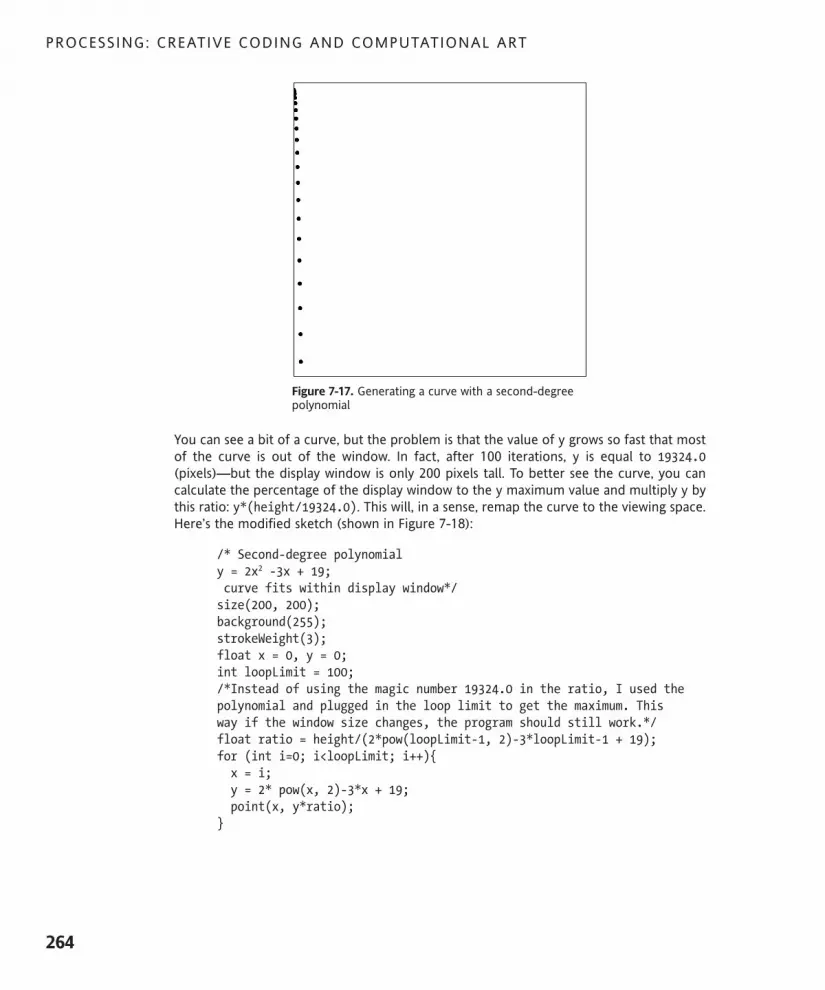
Figure 7-17. Generating a curve with a second-degree polynomial
You can see a bit of a curve, but the problem is that the value of y grows so fast that mostof the curve is out of the window. In fact, after 100 iterations, y is equal to 19324.0(pixels)—but the display window is only 200 pixels tall. To better see the curve, you cancalculate the percentage of the display window to the y maximum value and multiply y bythis ratio: y*(height/19324.0). This will, in a sense, remap the curve to the viewing space.Here’s the modified sketch (shown in Figure 7-18):
/* Second-degree polynomialy = 2x2 -3x + 19;curve fits within display window*/size(200, 200);background(255);strokeWeight(3);float x = 0, y = 0;int loopLimit = 100;/*Instead of using the magic number 19324.0 in the ratio, I used thepolynomial and plugged in the loop limit to get the maximum. Thisway if the window size changes, the program should still work.*/float ratio = height/(2*pow(loopLimit-1, 2)-3*loopLimit-1 + 19);for (int i=0; i<loopLimit; i++){x = i;y = 2* pow(x, 2)-3*x + 19;point(x, y*ratio);
}
PROCESSING: CREATIVE CODING AND COMPUTATIONAL ART
264
617xCH07.qxd 4/17/07 1:38 PM Page 264

Figure 7-18. Generating a curve with a second-degree polynomial, mapped to the display window
The scary-looking line float ratio = height/(2*pow(loopLimit-1, 2)-3*loopLimit-1+ 19); is your quadratic equation converted into code. The pow(loopLimit-1, 2) partuses Processing’s built-in pow() function. The function takes two arguments: the first is thevalue to act upon (the base), and the second is the power to raise the value to (the expo-nent), so pow(loopLimit-1, 2) is equal to (loopLimit – 1)2. In this case, the base is theexpression loopLimit – 1.
There is another important property of second-degree polynomials, also known asquadratic curves, that you’re not seeing in the plot. Quadratics don’t just form any oldcurves—they form parabolas, or bell-shaped symmetrical curves. However, to see the bellshape, you need to shift the curve to the right by width/2, and also begin your for loop at-width/2. Here’s the modified sketch code (shown in Figure 7-19):
/* parabolay = 2x2 -3x + 19;parabola fits within display window*/size(400, 400);background(255);strokeWeight(3);float x = 0, y = 0;int loopLimit = 200;//shifts curve to the rightint xShift = width/2;/*Instead of using the magic number 19324.0 in the ratio, I used thepolynomial and plugged in the loop limit to get the maximum. Thisway if the window size changes, the program should still work.*/float ratio = height/(2*pow(loopLimit-1, 2)-3*loopLimit-1 + 19);
CURVES
265
7
617xCH07.qxd 4/17/07 1:38 PM Page 265

for (int i=-xShift; i<loopLimit; i++){x = i;y = 2* pow(x, 2)-3*x + 19;point(x+xShift, y*ratio);
}
Figure 7-19. Generating a parabola with a quadratic curve
If all this math is making your eyes glaze over (sorry), we’re almost done. Curves are not sosimple, even using Processing’s built-in functions, as you’ll see shortly. But it’s helpful tohave some sense of what’s happening under the hood. The last curve equation I’ll look atbriefly is a third-degree polynomial, or cubic curve. These curves, like quadratics, are fun-damental to computer graphics. Cubic curves give you one additional feature that quad-ratic curves don’t, and that is a point of inflection. Inflection means the curve changesdirection. Think of the difference between the letters C (quadratic curve) and S (cubiccurve); the S contains an inflection point. What’s really significant about this change ofdirection, with regard to polynomials, is that it’s always a smooth transition.
Higher-degree polynomials (above third-degree) will also include inflection points, butthey require more processing power to calculate, and are ultimately harder to control.Thus, most curved lines and surfaces in computer graphics rely in some way on quadraticand cubic curves. This last polynomial example generates a cubic curve from the equationy = 4x3 – 6x2 + 3x – 20. I’ve taken the liberty of shifting and scaling the output so that it fitshappily within the display window, as shown in Figure 7-20.
/* Third-degree polynomialy = 4x3-6x2+3x-20*/size(400, 400);background(255);strokeWeight(3);smooth();
PROCESSING: CREATIVE CODING AND COMPUTATIONAL ART
266
617xCH07.qxd 4/17/07 1:38 PM Page 266

float x = 0, y = 0;int loopLimit = 200;//shifts curve to the rightint xShift = width/2;//shifts curve downint yShift = height/2;//fits curve to windowfloat ratio = height/(4* pow(loopLimit-1, 3)-6*pow(loopLimit-1, 2) !+ 3*loopLimit-1 - 20);
for (int i=-xShift; i<loopLimit; i++){x = i;y = 4* pow(x, 3)-6*pow(x, 2) + 3*x - 20;point(x+xShift, y*ratio+yShift);
}
Figure 7-20. Plot of a cubic curve (third-degree polynomial)
Using Processing’s curve functionsCongratulations! You just made it through the scary math section of the chapter. It onlygets easier from here. It’s time to look at Processing’s built-in curve functions. TheProcessing language reference includes numerous functions dealing with curves, allhoused under the Shape subheading. These functions simplify curve generation, handlingmost of the scary math internally. Within the Shape section is a section called Curves,which includes eight curve functions. In addition, in the Vertex section are two more vertexcurve functions. Finally, there’s one other lonely curve function hanging out in the 2DPrimitives section, called arc(), which I’ll begin with.
CURVES
267
7
617xCH07.qxd 4/17/07 1:38 PM Page 267
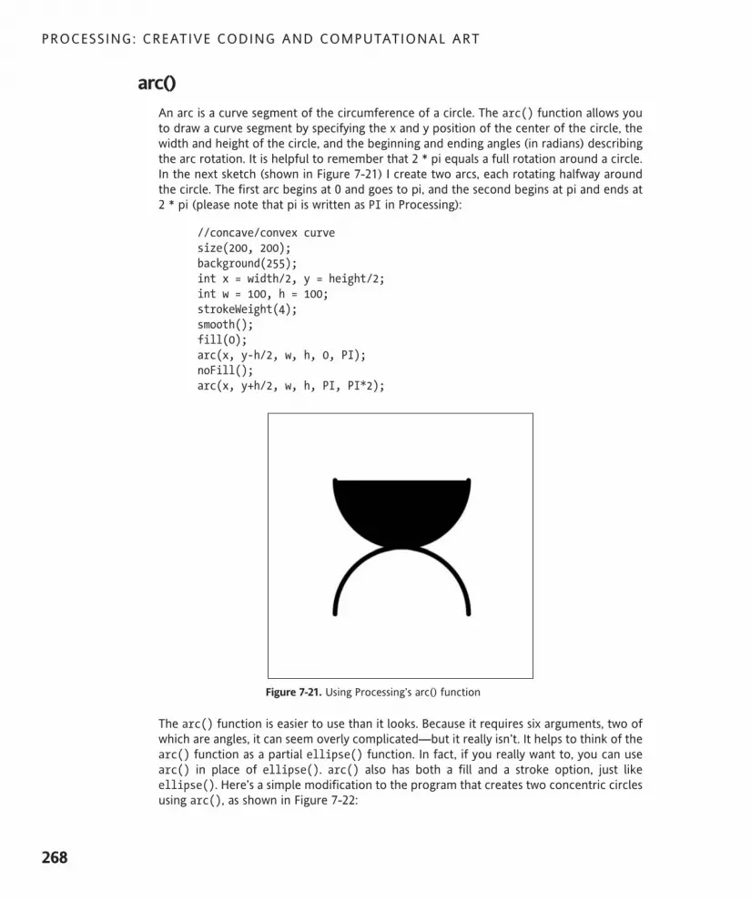
arc()An arc is a curve segment of the circumference of a circle. The arc() function allows youto draw a curve segment by specifying the x and y position of the center of the circle, thewidth and height of the circle, and the beginning and ending angles (in radians) describingthe arc rotation. It is helpful to remember that 2 * pi equals a full rotation around a circle.In the next sketch (shown in Figure 7-21) I create two arcs, each rotating halfway aroundthe circle. The first arc begins at 0 and goes to pi, and the second begins at pi and ends at2 * pi (please note that pi is written as PI in Processing):
//concave/convex curvesize(200, 200);background(255);int x = width/2, y = height/2;int w = 100, h = 100;strokeWeight(4);smooth();fill(0);arc(x, y-h/2, w, h, 0, PI);noFill();arc(x, y+h/2, w, h, PI, PI*2);
Figure 7-21. Using Processing’s arc() function
The arc() function is easier to use than it looks. Because it requires six arguments, two ofwhich are angles, it can seem overly complicated—but it really isn’t. It helps to think of thearc() function as a partial ellipse() function. In fact, if you really want to, you can usearc() in place of ellipse(). arc() also has both a fill and a stroke option, just likeellipse(). Here’s a simple modification to the program that creates two concentric circlesusing arc(), as shown in Figure 7-22:
PROCESSING: CREATIVE CODING AND COMPUTATIONAL ART
268
617xCH07.qxd 4/17/07 1:38 PM Page 268

//concentric circlessize(200, 200);background(255);int x = width/2, y = height/2;int w = 100, h = 100;strokeWeight(4);smooth();fill(0);arc(x, y, w-50, h-50, 0, PI*2);noFill();arc(x, y, w, h, 0, TWO_PI);
Figure 7-22. Creating circles with arc()
The arc() function’s first four arguments are identical to ellipse()’s arguments: x, y,width, and height. You can also specify an ellipseMode() when using arc() to controlfrom what point the arc is drawn; the default mode is CENTER. The arc() function’s lasttwo arguments are the start and end angles of the arc’s rotation, specified in radians. Ifyou prefer to work in degrees, just convert the degrees to radians, using theradians(angle) function. You’ll notice in my examples that I used PI as my value of rota-tion. PI, in radians, specifies 180 degree rotation around an ellipse. PI*2, in radians, givesone complete rotation (360 degrees). Processing actually has a constant for this as well:TWO_PI, which I used in the second arc() statement.
Although arc() is easy to use, it is somewhat lacking as a general-purpose curve tool. Forexample, to create a continuous curve path, it’s a little annoying trying to get a series ofarcs to line up. I’ll look at other Processing curve functions that do a better job with that.One cool thing you can do with arc() is make wedge shapes. A not-so-exciting applicationof this would be your standard pie chart. Here’s a simple example (shown in Figure 7-23):
CURVES
269
7
617xCH07.qxd 4/17/07 1:38 PM Page 269

//pie chartsize(400, 400);background(0);smooth();stroke(127);fill(0);int radius = 150;int[]angs = {40, 10, 20, 35, 55, 30, 60, 110};float lastAng = 0;for (int i=0; i<angs.length; i++){fill(random(255));arc(width/2, height/2, radius*2, radius*2, lastAng, !lastAng+=radians(angs[i]));
}
Figure 7-23. Simple pie chart
There’s nothing too earth shattering about this last example. One subtle issue, though,which can really mess things up if not handled properly, is the correct use of data types incalculations. After running the pie chart sketch a few times, switch the data type of thelastAng variable from float to int and run the program again. You won’t get any com-piler errors, but you’ll notice that only a partial pie forms. To better understand how a sub-tle change like this can wreck your pretty pie chart, add println(lastAng) below thearc() call, and try both data types again. When lastAng is declared as an int, println()outputs 0, 0, 0, 0, 0, 0, 1, 2; when declared as a float instead, the output is 0.698...,0.873..., 1.222..., 1.833..., 2.793..., 3.316..., 4.363..., 6.283.... Thereason for the discrepancy is that when lastAng is declared as an int, the linelastAng+=radians(angs[i]) rounds down the value of radians(angs[i]) from a floatvalue to an int—so anything under 1.0 becomes 0, anything between 1.0 and 2.0 becomes1.0, and so on.
PROCESSING: CREATIVE CODING AND COMPUTATIONAL ART
270
617xCH07.qxd 4/17/07 1:38 PM Page 270

Pie charts, although valuable as visualization tools, don’t do much for me. The next sketch,shown in Figure 7-24, is a progression of a pie wedge from a thin fragment to a full pie. Ialso incremented the value of the wedge fill color.
//Progressive Arcssize(400, 400);background(50);smooth();noStroke();float diameter = 40;float ang = 0;float col = 0;float xCount = width/diameter;float yCount = height/diameter;float cellTotal = xCount*yCount;float angIncrement = radians(360.0/cellTotal);float colIncrement = 255.0/cellTotal;for (float i=diameter/2; i<=height; i+=diameter){for (float j=diameter/2; j<=width; j+=diameter){
ang+=angIncrement;col += colIncrement;fill(col);arc(j, i, diameter, diameter, 0, ang);
}}
Figure 7-24. Progression of pie wedge shapes within a table structure
CURVES
271
7
617xCH07.qxd 4/17/07 1:38 PM Page 271

The sketch relies on a basic table structure made up of pie wedge shapes. There’s nothingnew here, as you’ve looked at similar code in earlier examples. The sketch is a little morevisually interesting than the pie chart, but can obviously be pushed further. By simplydecreasing the value of the diameter variable and adding some randomization, you canimprove the output quite a bit, as shown in Figure 7-25.
//Pie Fragmentssize(400, 400);background(255);smooth();noStroke();float radius = 10;for (int i=0; i<=width; i+=radius/2){for (int j=0; j<=height; j+=radius/2){float size = (random(radius*2));fill(255);arc(random(i), random(j), size, size, random(PI*2), random(PI*2));fill(0);arc(random(i), random(j), size, size, random(PI*2), random(PI*2));
}}
Figure 7-25. Randomized pie wedge texture
PROCESSING: CREATIVE CODING AND COMPUTATIONAL ART
272
617xCH07.qxd 4/17/07 1:38 PM Page 272

curve() and bezier()The next two Processing curve functions I’ll look at are curve() and bezier(). I’ll considerthese functions together, as they share some common implementation issues. As you’veprobably gathered by now, the implementation of curves is a little complex. Fortunately,Processing’s curve() and bezier() functions simplify curve generation quite a bit. Thesefunctions encapsulate pretty sophisticated mathematical ideas, including cubic polynomi-als—which you looked at a little—as well as some calculus. I’m not going to deal with thecalculus here, nor mess directly with polynomials. The functions each require eight argu-ments, representing the x and y components of four points. The bezier() function usestwo points (the first two parameters and the last two parameters) to describe the ends ofthe curves (anchor points), and two additional points (the middle four parameters) to con-trol how the curve moves between the endpoints (referred to as control points). Here’s anexample (shown in Figure 7-26). Please note that I took the liberty of connecting the con-trol and anchor points with lines to help illustrate how the structure works.
//Bézier sketchsize(400, 400);background(255);smooth();/*I used Java's Point class, a convenientdata type for holding x,y coords, with publicaccess to x and y properties (pt.x or pt.y)*/Point pt1 = new Point(150, 300);Point pt2 = new Point(100, 100);Point pt3 = new Point(300, 100);Point pt4 = new Point(250, 300);//plot curvestroke(0);bezier(pt1.x, pt1.y, pt2.x, pt2.y, pt3.x, pt3.y, pt4.x, pt4.y);//draw control points connected to anchor pointsstroke(150);line(pt1.x, pt1.y, pt2.x, pt2.y);line(pt3.x, pt3.y, pt4.x, pt4.y);//control pointsellipse(pt2.x, pt2.y, 10, 10);ellipse(pt3.x, pt3.y, 10, 10);//anchor pointsrectMode(CENTER);rect(pt1.x, pt1.y, 10, 10);rect(pt4.x, pt4.y, 10, 10);
CURVES
273
7
617xCH07.qxd 4/17/07 1:38 PM Page 273

Figure 7-26. Bézier curve plot showing anchor and control points
I utilized Java’s Point class in the example as a simple data structure. The Point class is notpart of the Processing API, but I find it handy to use because it provides direct access to anx and a y property, which I used to help keep track of the different anchor and controlpoints. You can create a new Point object by simply writing Point pt1 = new Point(150,300);. The two arguments you pass, 150 and 300, will be the values of the x and y proper-ties, respectively. So, to access the x and y values, I just write pt1.x and pt1.y. The rest ofthe code in the sketch is stuff you’ve seen numerous times before in earlier examples (andwill see a lot more of).
If you’ve ever used a pen tool in a graphics application like Illustrator, Photoshop, orFreeHand (and I assume most of you have), then you’ve experienced Bézier curves, andmaybe you’ve even messed directly with their control points. Bézier curves are namedafter Pierre Bézier, a French mathematician and engineer who worked for the car manu-facturer Renault. To learn more about Bézier and his curve, check out http://cg.scs.carleton.ca/~luc/bezier.html.
There is a dynamic tension in a Bézier curve, determined by the placement of the controlpoints (the small ellipse handles in the example) and their relative position to the anchorpoints (the small squares at ends of curve). You’ll notice in the example that the curveseems to bend toward the control points. The situation is actually a little more compli-cated than that. The extra lines I rendered between the control points and the anchorpoints represent the slopes of the curves at the anchor points (also known as tangentlines). Slope is the change in y over the change in x (the rise over the run). Finding slopesof curves is a little tricky, since the curves are constantly changing, unlike straight lines, inwhich the slope is constant. On curves, you can take slope readings at distinct points. Fora more generalized approach to solving for the slope of a curve, you need basic calculus—so I’ll stop there. In a sense, the Bézier curve between the two anchor points is calculatedby blending, or interpolating, the two slopes of the curve at the anchor points, as well asfactoring in the distance between the anchor and control points.
PROCESSING: CREATIVE CODING AND COMPUTATIONAL ART
274
617xCH07.qxd 4/17/07 1:38 PM Page 274

Next is an interactive example that illustrates this interpolation process as a simple geo-metric progression. The sketch (shown in Figure 7-27) plots a quadratic curve using twoanchor points and a single control point, and interpolates between these three points.Technically, the area defined by the control and anchor points is called a convex hull. Eachtime you click within the example, another iteration occurs, dividing the previous seg-ments in half and plotting the path, slowly approximating the curve.
/* Interpolating a Béziercurve within a convex hull **************************Click the screen a couple oftimes to iteratively generatethe curve*/
int startingPoints = 3;// Uses Java's Point classPoint[] bezier = new Point[startingPoints];
void setup(){size(600, 400);background(255);smooth();// create external bezierbezier[0] = new Point(10, 390);bezier[1] = new Point(300, 10);bezier[2] = new Point(590, 390);// plot initial convex hullplot(bezier);
}
Point[] plotBezier(Point[] pts){Point[] path = new Point[pts.length+1];path[0] = pts[0];for (int i=1; i<path.length-1; i++){ path[i] = new Point((pts[i-1].x+pts[i].x)/2, !(pts[i-1].y+pts[i].y)/2);
}path[path.length-1] = pts[pts.length-1];plot(path);return path;
}
void plot(Point[] pts){/*** render hull ***/if (pts.length==startingPoints){noFill();stroke(0);strokeWeight(2);//path
CURVES
275
7
617xCH07.qxd 4/17/07 1:38 PM Page 275

beginShape();for (int i=0; i<pts.length; i++){vertex(pts[i].x, pts[i].y);
}endShape();
//pointsfill(255);for (int i=0; i<pts.length; i++){if (i>0 && i<pts.length-1){rectMode(CENTER);// control pointrect(pts[i].x, pts[i].y, 12, 12);
}else {// anchor pointsellipse(pts[i].x, pts[i].y, 12, 12);
}}
}/*** render interpolated path ***/else {// pathnoFill();stroke(100);strokeWeight(1);beginShape();for (int i=1; i<pts.length-1; i++){vertex(pts[i].x, pts[i].y);
}endShape();// pointsfill(0);for (int i=1; i<pts.length-1; i++){ellipse(pts[i].x, pts[i].y, 4, 4);
}}
}
/* draw function required whenincluding mousePressed function*/void draw(){}void mousePressed(){bezier = plotBezier(bezier);
}
PROCESSING: CREATIVE CODING AND COMPUTATIONAL ART
276
617xCH07.qxd 4/17/07 1:38 PM Page 276

Figure 7-27. Interpolating a Bézier curve within a convex hull
There’s nothing new in the last sketch, but I hope it illustrates how the convex hull (theshape defined by the three initial points) dictates the placement and shape of the curve.You can use this same sketch to approximate a cubic Bézier curve as well, with four initialpoints instead of three. You’ll remember that cubic curves can contain an inflection pointin the curve, or a change in direction, as shown in Figure 7-28. To generate this image,simply make the following changes to the values in the last sketch, and rerun it:
int startingPoints = 4;
bezier[0] = new Point(200, 700);bezier[1] = new Point(100, 50);bezier[2] = new Point(1100, 750);bezier[3] = new Point(1000, 100);
CURVES
277
7
617xCH07.qxd 4/17/07 1:38 PM Page 277
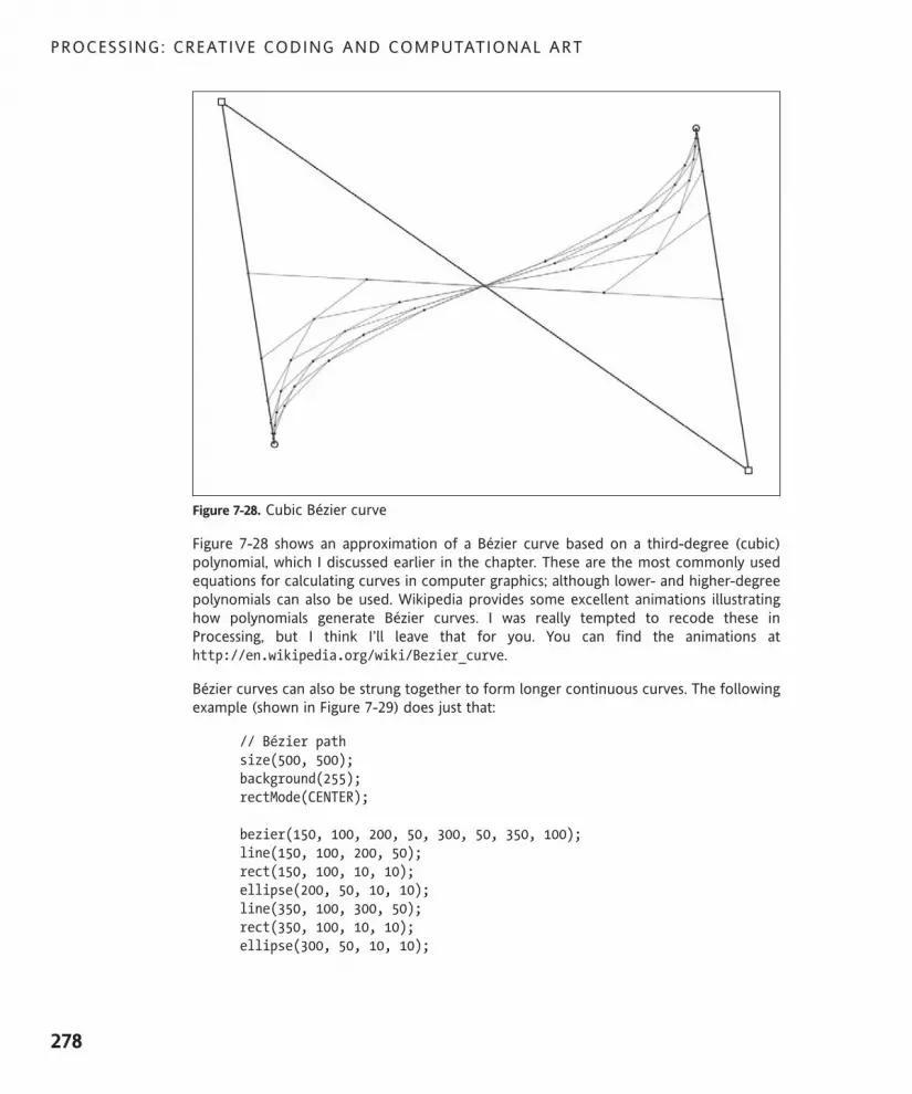
Figure 7-28. Cubic Bézier curve
Figure 7-28 shows an approximation of a Bézier curve based on a third-degree (cubic)polynomial, which I discussed earlier in the chapter. These are the most commonly usedequations for calculating curves in computer graphics; although lower- and higher-degreepolynomials can also be used. Wikipedia provides some excellent animations illustratinghow polynomials generate Bézier curves. I was really tempted to recode these inProcessing, but I think I’ll leave that for you. You can find the animations athttp://en.wikipedia.org/wiki/Bezier_curve.
Bézier curves can also be strung together to form longer continuous curves. The followingexample (shown in Figure 7-29) does just that:
// Bézier pathsize(500, 500);background(255);rectMode(CENTER);
bezier(150, 100, 200, 50, 300, 50, 350, 100);line(150, 100, 200, 50);rect(150, 100, 10, 10);ellipse(200, 50, 10, 10);line(350, 100, 300, 50);rect(350, 100, 10, 10);ellipse(300, 50, 10, 10);
PROCESSING: CREATIVE CODING AND COMPUTATIONAL ART
278
617xCH07.qxd 4/17/07 1:38 PM Page 278

bezier(350, 100, 400, 150, 350, 250, 350, 300);line(350, 100, 400, 150);rect(350, 100, 10, 10);ellipse(400, 150, 10, 10);line(350, 300, 350, 250);rect(350, 300, 10, 10);ellipse(350, 250, 10, 10);
bezier(350, 300, 300, 350, 100, 250, 100, 400);line(350, 300, 300, 350);rect(350, 300, 10, 10);ellipse(300, 350, 10, 10);line(100, 400, 100, 250);rect(100, 400, 10, 10);ellipse(100, 250, 10, 10);
Figure 7-29. Connecting Bézier curves together
In this last example, notice how the control handles change the curve. The control handlesthat are aligned, forming a straight line at the second anchor point, generate a reallysmooth curve segment. However, the next anchor point forms a cusp, or kink, in the curve,as the handles don’t align. This independence of the two control handles is both a benefitand liability of using Bézier curves. Cusps in the curve can translate to jerky motion inobject or camera animations in 3D animation programs, or create an unwanted detail in avector illustration or typeface design. However, in spite of these challenges, Bézier curvesare very efficient, with a lot of descriptive capabilities, and are used widely in computergraphics.
CURVES
279
7
617xCH07.qxd 4/17/07 1:38 PM Page 279

Another way you can generate more complex curves, without depending solely on string-ing so many Bézier segments together, is to use higher-degree polynomials. Higher-degreecurves provide more inflection points (the places where curves change direction), and alsorequire more control points. The number of control points is determined by the polyno-mial degree minus 1—that’s why the standard Bézier, third-degree curve has two controlhandles. The ability for a curve to change direction a number of times should make it use-ful as a design or animation tool. However, the complexity and computational cost ofusing these higher-degree curves offsets most of the benefits. Thus, you’re pretty muchstuck with the cubic (third-degree) and quadratic (second-degree) curves you’ve alreadylooked at.
However, there is one other important approach to creating smooth, continuous curvesthat simplifies some of the challenges of simply stringing together Bézier curves. Thisapproach is encapsulated (within Processing) in the curve() function. I’ll show you howthe curve() function actually works in a minute, but first I’ll jump in with a curve() exam-ple (see Figure 7-30) that plots the same curve generated in the preceding Bézier exampleto help highlight the difference between the two functions:
// Catmull-Rom spline curvesize(500, 500);background(255);
Point p0 = new Point(150, 100);Point p1 = new Point(350, 100);Point p2 = new Point(350, 300);Point p3 = new Point(150, 300);Point p4 = new Point(100, 400);
//curve segmentscurve(p4.x, p4.y, p0.x, p0.y, p1.x, p1.y, p2.x, p2.y);curve(p0.x, p0.y, p1.x, p1.y, p2.x, p2.y, p3.x, p3.y);curve(p1.x, p1.y, p2.x, p2.y, p3.x, p3.y, p4.x, p4.y);curve(p2.x, p2.y, p3.x, p3.y, p4.x, p4.y, p0.x, p0.y );
//control pointsellipse(p0.x, p0.y, 10, 10);ellipse(p1.x, p1.y, 10, 10);ellipse(p2.x, p2.y, 10, 10);ellipse(p3.x, p3.y, 10, 10);ellipse(p4.x, p4.y, 10, 10);
PROCESSING: CREATIVE CODING AND COMPUTATIONAL ART
280
617xCH07.qxd 4/17/07 1:38 PM Page 280

The curve() function is a spline curve implementation, or more precisely a Catmull-Romspline implementation. The name “Catmull-Rom” comes from computer scientists EdwinCatmull and Raphael Rom. Catmull later went on to establish a small independent anima-tion studio in 1986, called Pixar. Thus, you might assume that Catmull-Rom splines are rel-evant to 3D animation—and you’d be right. They’re important for efficiently generatingcomplex, smooth geometry—creating motion paths, among other things. In addition tocurve(), Processing has a related function, called vertexCurve(), that implements thesame Catmull-Rom spline. I think vertexCurve() is a little simpler to use than curve() (I’lllook at this function after I slog through the curve() function a bit).
In the last example, I created five initial points to hold the curves’ control points. Hopefullyyou noticed that there were no control points off the path, as in the earlier bezier()example. This is one of the main differences between a Bézier curve and a Catmull-Romspline curve. After creating the five points, I call my curve() functions. Like the bezier()function, curve() uses eight parameters—the x and y components of four points.However, unlike bezier(), curve() doesn’t use a system of anchor and control points.Instead, all four of the points, in a sense, function as control points. The curve then followsthe path of the control points. Look closely at the curve() calls in my last example. Herethey are again:
curve(p4.x, p4.y, p0.x, p0.y, p1.x, p1.y, p2.x, p2.y);curve(p0.x, p0.y, p1.x, p1.y, p2.x, p2.y, p3.x, p3.y);curve(p1.x, p1.y, p2.x, p2.y, p3.x, p3.y, p4.x, p4.y);curve(p2.x, p2.y, p3.x, p3.y, p4.x, p4.y, p0.x, p0.y);
In the first curve() call, points p0 and p1 are at the left and right edges of the first seg-ment of the curve. p4 and p2 are the extra control points on either side. In the nextcurve() call, I copy p1 to the left point position of the second curve. This will allow thefirst curve’s right point and the second curve’s left point to align. I then use p2 for the rightpoint of the second curve. Since each point also needs a control point on the left andright, I put p0 to the left of p1, and p3 to the right of p2. This same pattern repeats itself inthe next two calls. The only thing that may look odd is the last p0 in the final curve. Since
Figure 7-30.Spline curve using Processing’s curve() function
CURVES
281
7
617xCH07.qxd 4/17/07 1:38 PM Page 281

I used p4 to its left, I chose to go back to the beginning of my curve, ensuring that p4 hada control point to its right. (I know this is confusing and not intuitive at all.) One other littletrick that may make this more comprehensible is that if you copy the third through theeighth parameters of a curve() function call and paste them in another curve() call, thenthe curves will connect. You’ll still need to add a seventh and eighth parameter to this newcurve. Look at these two lines:
curve(p0.x, p0.y, p1.x, p1.y, p2.x, p2.y, p3.x, p3.y);curve(p1.x, p1.y, p2.x, p2.y, p3.x, p3.y);
Notice how the third through eighth parameters in the first curve() call repeat as the firstthrough the sixth parameters in the next curve() call. I still need to add the last twoparameters to the second curve, which I do by continuing the cycle from p3 to p4 for theseventh and eighth parameters:
curve(p0.x, p0.y, p1.x, p1.y, p2.x, p2.y, p3.x, p3.y);curve(p1.x, p1.y, p2.x, p2.y, p3.x, p3.y, p4.x, p4.y);
Finally, there is one other cool function available to control the tension of the spline curve;it works similarly to how control points on a Bézier curve exaggerate or flatten a curve,depending upon where the handles are located. Using curve(), you don’t literally drag anyhandles or set extra control points off the curve. Instead, you simply pass a value to thecurveTightness(value) function. The value can be negative or positive. In this next exam-ple (shown in Figure 7-31), I create a series of identical spline curves, with varying degreesof curve tightness, using the values -2, -1, 0, 1, and 2 as arguments in thecurveTightness(value) function (please note that you need to use Processing’s noFill()function if you don’t want your curves filling in):
// Catmull-Rom spline curve// Curve Tightnesssize(600, 400);background(0);stroke(255);strokeWeight(2);smooth();int curveWdth = 50;int cols = 5;int xPadding = (width-curveWdth*cols)/(cols+1);int x = xPadding;
for (int i=-2; i<3; i++){curveTightness(i);Point p0 = new Point(x, 100);Point p1 = new Point(x+curveWdth, 100);Point p2 = new Point(x+curveWdth, 300);Point p3 = new Point(x, 300);Point p4 = new Point(x, 200);x+=curveWdth+xPadding;
PROCESSING: CREATIVE CODING AND COMPUTATIONAL ART
282
617xCH07.qxd 4/17/07 1:38 PM Page 282

//curve segmentsnoFill(); // comment this line out to see how the curve fillscurve(p4.x, p4.y, p0.x, p0.y, p1.x, p1.y, p2.x, p2.y);curve(p0.x, p0.y, p1.x, p1.y, p2.x, p2.y, p3.x, p3.y);curve(p1.x, p1.y, p2.x, p2.y, p3.x, p3.y, p4.x, p4.y);curve(p2.x, p2.y, p3.x, p3.y, p4.x, p4.y, p0.x, p0.y );
//control pointsfill(255);ellipse(p0.x, p0.y, 5, 5);ellipse(p1.x, p1.y, 5, 5);ellipse(p2.x, p2.y, 5, 5);ellipse(p3.x, p3.y, 5, 5);ellipse(p4.x, p4.y, 5, 5);
}
Figure 7-31. Controlling curvature using Processing’s curveTightness() function
All right, so that covers most of the theory part of curves. I realize it may have been a bitrough to get through. One of my goals in this book is to try to provide detailed and clearexplanations of important concepts that are often not well articulated in existing sources(that I can find). For example, in doing research on splines, I was amazed at howinscrutable most of the explanations were. This was mostly due to the dense mathematicalexplanations. The concepts themselves aren’t that complicated, but when they’reexplained as a page of Greek symbols, matrices, and complex graphs, well—you’re notgoing to entice many artists. I also expect you to move through this material pretty quickly(on the first read through), mostly just remembering that it’s covered in the book. As youprogress in your work and develop more coding chops, there will be times you’llneed/want to deal with some of these more complex issues.
CURVES
283
7
617xCH07.qxd 4/17/07 1:38 PM Page 283

Next, I want to put this material to better use and cover just a few more curve functions.But don’t worry, most of the really difficult stuff is over (at least in this chapter). I won’tformally be covering interactivity until Chapter 12. However, it can be helpful in trying tounderstand curve concepts to be able to play around with the curves, including yanking ontheir control points. I’m not going to go into all the interactive theory here, so some of thecode in the upcoming interactive examples may look odd (and possibly scary). You canpeek ahead to Chapter 12 if you want to, but I’d suggest just playing with the stuff for now,and get to the learning part a little later. You’re entitled to fool around a bit, in blissfulignorance.
More curve and Bézier variationsThe next two examples, shown in Figures 7-32 and 7-33, are just variations on a theme.You’ll eventually use the bezier() function to plot a more ambitious sketch consisting ofa very interactive ellipse, which you’ll be able to mess around with in real time. Hopefullythis example will reveal some of the creative potential of having to deal with curve com-plexity. First, however, I’ll look at two more functions: bezierVertex() and curveVertex().These functions are really just alternative forms of the bezier() and curve() functions.The following example plots three spirals using the bezier() and bezierVertex() func-tions. Again, I’ve added extra code to render the control handles to show how their place-ment affects the spiral. I didn’t bother to render the anchor points in this example, and Ialso doubled up the line() and ellipse() calls to save a few trees.
// bezier() vs. bezierVertex()size(650, 225);background(255);rectMode(CENTER);strokeWeight(2);
//bezier() - no fillnoFill();bezier(50, 50, 92, 15, 134, 15, 175, 50);bezier(175, 50, 215, 92, 215, 134, 175, 175);bezier(175, 175, 135, 205, 105, 205, 75, 175);bezier(75, 175, 50, 145, 50, 105, 75, 75);bezier(75, 75, 100, 54, 125, 54, 150, 75);bezier(150, 75, 175, 100, 175, 125, 150, 150);bezier(150, 150, 134, 160, 118, 160, 100, 150);bezier(100, 150, 92, 140, 92, 130, 100, 115);
//lines connecting anchor points to control handlesstrokeWeight(1);line(50, 50, 92, 15); line(134, 15, 175, 50);line(175, 50, 215, 92); line(215, 134, 175, 175);line(175, 175, 135, 205); line(105, 205, 75, 175);line(75, 175, 50, 145); line(50, 105, 75, 75);line(75, 75, 100, 54); line(125, 54, 150, 75);line(150, 75, 175, 100); line(175, 125, 150, 150);line(150, 150, 134, 160); line(118, 160, 100, 150);line(100, 150, 92, 140); line(92, 130, 100, 115);
PROCESSING: CREATIVE CODING AND COMPUTATIONAL ART
284
617xCH07.qxd 4/17/07 1:38 PM Page 284

//control handlesfill(255);ellipse(92, 15, 8, 8); ellipse(134, 15, 8, 8);ellipse(215, 92, 8, 8); ellipse(215, 134, 8, 8);ellipse(135, 205, 8, 8); ellipse(105, 205, 8, 8);ellipse(50, 145, 8, 8); ellipse(50, 105, 8, 8);ellipse(100, 54, 8, 8); ellipse(125, 54, 8, 8);ellipse(175, 100, 8, 8); ellipse(175, 125, 8, 8);ellipse(134, 160, 8, 8); ellipse(118, 160, 8, 8);ellipse(92, 140, 8, 8); ellipse(92, 130, 8, 8);
//bezierVertex() - closed and no fillstrokeWeight(2);int x = 200;noFill();beginShape();vertex(50+x, 50);bezierVertex(92+x, 15, 134+x, 15, 175+x, 50);bezierVertex(215+x, 92, 215+x, 134, 175+x, 175);bezierVertex(135+x, 205, 105+x, 205, 75+x, 175);bezierVertex(50+x, 145, 50+x, 105, 75+x, 75);bezierVertex(100+x, 54, 125+x, 54, 150+x, 75);bezierVertex(175+x, 100, 175+x, 125, 150+x, 150);bezierVertex(134+x, 160, 118+x, 160, 100+x, 150);bezierVertex(92+x, 140, 92+x, 130, 100+x, 115);endShape(CLOSE);
//lines connecting anchor points to control handlesstrokeWeight(1);stroke(0);line(50+x, 50, 92+x, 15); line(134+x, 15, 175+x, 50);line(175+x, 50, 215+x, 92); line(215+x, 134, 175+x, 175);line(175+x, 175, 135+x, 205); line(105+x, 205, 75+x, 175);line(75+x, 175, 50+x, 145); line(50+x, 105, 75+x, 75);line(75+x, 75, 100+x, 54); line(125+x, 54, 150+x, 75);line(150+x, 75, 175+x, 100); line(175+x, 125, 150+x, 150);line(150+x, 150, 134+x, 160); line(118+x, 160, 100+x, 150);line(100+x, 150, 92+x, 140); line(92+x, 130, 100+x, 115);
//control handlesfill(255);ellipse(92+x, 15, 8, 8); ellipse(134+x, 15, 8, 8);ellipse(215+x, 92, 8, 8); ellipse(215+x, 134, 8, 8);ellipse(135+x, 205, 8, 8); ellipse(105+x, 205, 8, 8);ellipse(50+x, 145, 8, 8); ellipse(50+x, 105, 8, 8);ellipse(100+x, 54, 8, 8); ellipse(125+x, 54, 8, 8);ellipse(175+x, 100, 8, 8); ellipse(175+x, 125, 8, 8);ellipse(134+x, 160, 8, 8); ellipse(118+x, 160, 8, 8);ellipse(92+x, 140, 8, 8); ellipse(92+x, 130, 8, 8);
CURVES
285
7
617xCH07.qxd 4/17/07 1:38 PM Page 285

//bezierVertex() - open and filledstrokeWeight(2);x = 400;fill(127);beginShape();vertex(50+x, 50);bezierVertex(92+x, 15, 134+x, 15, 175+x, 50);bezierVertex(215+x, 92, 215+x, 134, 175+x, 175);bezierVertex(135+x, 205, 105+x, 205, 75+x, 175);bezierVertex(50+x, 145, 50+x, 105, 75+x, 75);bezierVertex(100+x, 54, 125+x, 54, 150+x, 75);bezierVertex(175+x, 100, 175+x, 125, 150+x, 150);bezierVertex(134+x, 160, 118+x, 160, 100+x, 150);bezierVertex(92+x, 140, 92+x, 130, 100+x, 115);endShape();
//lines connecting anchor points to control handlesstrokeWeight(1);stroke(0);line(50+x, 50, 92+x, 15); line(134+x, 15, 175+x, 50);line(175+x, 50, 215+x, 92); line(215+x, 134, 175+x, 175);line(175+x, 175, 135+x, 205); line(105+x, 205, 75+x, 175);line(75+x, 175, 50+x, 145); line(50+x, 105, 75+x, 75);line(75+x, 75, 100+x, 54); line(125+x, 54, 150+x, 75);line(150+x, 75, 175+x, 100); line(175+x, 125, 150+x, 150);line(150+x, 150, 134+x, 160); line(118+x, 160, 100+x, 150);line(100+x, 150, 92+x, 140); line(92+x, 130, 100+x, 115);
//control handlesfill(255);ellipse(92+x, 15, 8, 8); ellipse(134+x, 15, 8, 8);ellipse(215+x, 92, 8, 8); ellipse(215+x, 134, 8, 8);ellipse(135+x, 205, 8, 8); ellipse(105+x, 205, 8, 8);ellipse(50+x, 145, 8, 8); ellipse(50+x, 105, 8, 8);ellipse(100+x, 54, 8, 8); ellipse(125+x, 54, 8, 8);ellipse(175+x, 100, 8, 8); ellipse(175+x, 125, 8, 8);ellipse(134+x, 160, 8, 8); ellipse(118+x, 160, 8, 8);ellipse(92+x, 140, 8, 8); ellipse(92+x, 130, 8, 8);
PROCESSING: CREATIVE CODING AND COMPUTATIONAL ART
286
617xCH07.qxd 4/17/07 1:38 PM Page 286

Figure 7-32. bezier() vs. bezierVertex() sketch
The bezierVertex() function needs to be called between beginShape() and endShape(),with the initial call being a single vertex() call. Remember that beginShape() beginsrecording coordinate data until endShape() is called, at which time the data is rendered tothe screen and filled by default. Although the shape will be filled, the path defining theshape will not be closed unless the CLOSE argument is included in the endShape(CLOSE)call. Of course, visually, you can make the path appear closed by making sure that theanchor point in the last bezierVertex(controPt1, controlPt2, anchorPt) call is placedat the same coordinate location as the initial vertex(x, y) call. If the starting and endingpoints are not in the same location, using the CLOSE argument will connect the two pointswith a straight line, which is what occurs in the second spiral in the last example. Bydefault, the shape will be filled following the same rule, as illustrated in the third spiral,even though this spiral is technically not closed. This same pattern of rules holds true forthe curve() and curveVertex() functions. For the sake of thoroughness, here’s acurve()/curveVertex() version of the last example:
//curve() vs. curveVertex()size(650, 225);background(255);rectMode(CENTER);strokeWeight(2);
//curve()noFill();curve(92, 15, 92, 15, 134, 15, 175, 50);curve(92, 15, 134, 15, 175, 50, 175, 175);curve(134, 15, 175, 50, 175, 175, 75, 175);curve(175, 50, 175, 175, 75, 175, 75, 75);curve(175, 175, 75, 175, 75, 75, 150, 75);curve(75, 175, 75, 75, 150, 75, 150, 150);curve(75, 75, 150, 75, 150, 150, 100, 150);curve(150, 75, 150, 150, 100, 150, 100, 150);
CURVES
287
7
617xCH07.qxd 4/17/07 1:38 PM Page 287

//control pointsstrokeWeight(1);fill(255);ellipse(92, 15, 8, 8);ellipse(134, 15, 8, 8);ellipse(175, 50, 8, 8);ellipse(175, 175, 8, 8);ellipse(75, 175, 8, 8);ellipse(75, 75, 8, 8);ellipse(150, 75, 8, 8);ellipse(150, 150, 8, 8);ellipse(100, 150, 8, 8);
//curveVertex - closed and unfilledstrokeWeight(2);int x = 200;beginShape();curveVertex(92+x, 15);curveVertex(92+x, 15);curveVertex(134+x, 15);curveVertex(175+x, 50);curveVertex(175+x, 175);curveVertex(75+x, 175);curveVertex(75+x, 75);curveVertex(150+x, 75);curveVertex(150+x, 150);curveVertex(100+x, 150);curveVertex(100+x, 150);endShape(CLOSE);
//control handlesstrokeWeight(1);fill(255);ellipse(92+x, 15, 8, 8);ellipse(134+x, 15, 8, 8);ellipse(175+x, 50, 8, 8);ellipse(175+x, 175, 8, 8);ellipse(75+x, 175, 8, 8);ellipse(75+x, 75, 8, 8);ellipse(150+x, 75, 8, 8);ellipse(150+x, 150, 8, 8);ellipse(100+x, 150, 8, 8);
//curveVertex() - open and filledx = 400;strokeWeight(2);fill(127);beginShape();
PROCESSING: CREATIVE CODING AND COMPUTATIONAL ART
288
617xCH07.qxd 4/17/07 1:38 PM Page 288

curveVertex(92+x, 15);curveVertex(92+x, 15);curveVertex(134+x, 15);curveVertex(175+x, 50);curveVertex(175+x, 175);curveVertex(75+x, 175);curveVertex(75+x, 75);curveVertex(150+x, 75);curveVertex(150+x, 150);curveVertex(100+x, 150);curveVertex(100+x, 150);endShape();
//control handlesstrokeWeight(1);fill(255);ellipse(92+x, 15, 8, 8);ellipse(134+x, 15, 8, 8);ellipse(175+x, 50, 8, 8);ellipse(175+x, 175, 8, 8);ellipse(75+x, 175, 8, 8);ellipse(75+x, 75, 8, 8);ellipse(150+x, 75, 8, 8);ellipse(150+x, 150, 8, 8);ellipse(100+x, 150, 8, 8);
Figure 7-33. curve() vs. curveVertex() sketch
I think the curveVertex() function is less work to use than curve(). Obviously, having todeal with two arguments is definitely better than eight. From bezier() to bezierVertex(),you go from eight to six arguments, so I’m not so sure for normal open paths if there ismuch advantage. For closed or fill paths, you’ll want to use bezierVertex() orcurveVertex(). Although you can fill individual bezier() and curve() curves, the fillwon’t span multiple connected curve segments. To see an example of this, replace thenoFill() call with fill(127) before the first spiral code in either of the last twoexamples.
CURVES
289
7
617xCH07.qxd 4/17/07 1:38 PM Page 289

One interesting thing to do with both the bezier() and curve() functions is to createelliptical plots, where the control points can be manipulated to create various intercon-nected curve patterns. The following example (shown in Figure 7-34) allows you to clickthe screen to generate a random ellipse pattern. I’ve also a coded a more advanced, highlyinteractive version of the example (shown in Figure 7-35), entitled Interactive BézierEllipse, which you can download from the Download section on the friends of ED site(www.friendsofed.com).
/*Bézier EllipseIra Greenberg, December 19, 2005Revised: November 15, 2006*/
// arrays to hold ellipse coordinate datafloat[] px, py, cx, cy, cx2, cy2;
// global variable - points in ellipseint pts = 4;
color controlPtCol = #222222;color anchorPtCol = #BBBBBB;
void setup(){size(600, 600);setEllipse(pts, 130, 130);
}
void draw(){background(145);drawEllipse();
}
// draw ellipse with anchor/control pointsvoid drawEllipse(){strokeWeight(1.125);stroke(255);noFill();// create ellipsefor (int i=0; i<pts; i++){if (i==pts-1) {bezier(px[i], py[i], cx[i], cy[i], cx2[i], cy2[i], !px[0], py[0]);
}else{bezier(px[i], py[i], cx[i], cy[i], cx2[i], cy2[i], !px[i+1], py[i+1]);
}}
PROCESSING: CREATIVE CODING AND COMPUTATIONAL ART
290
617xCH07.qxd 4/17/07 1:38 PM Page 290

strokeWeight(.75);stroke(0);rectMode(CENTER);
// control handles and tangent linesfor (int i=0; i<pts; i++){if (i==pts-1){ // last loop iteration - close pathline(px[0], py[0], cx2[i], cy2[i]);
}if (i>0){line(px[i], py[i], cx2[i-1], cy2[i-1]);
}line(px[i], py[i], cx[i], cy[i]);
}
for (int i=0; i<pts; i++){fill(controlPtCol);noStroke();//control handlesellipse(cx[i], cy[i], 4, 4);ellipse(cx2[i], cy2[i], 4, 4);
fill(anchorPtCol);stroke(0);//anchor pointsrect(px[i], py[i], 5, 5);
}}
// fill up arrays with ellipse coordinate datavoid setEllipse(int points, float radius, float controlRadius){pts = points;px = new float[points];py = new float[points];cx = new float[points];cy = new float[points];cx2 = new float[points];cy2 = new float[points];float angle = 360.0/points;float controlAngle1 = angle/3.0;float controlAngle2 = controlAngle1*2.0;for (int i=0; i<points; i++){px[i] = width/2+cos(radians(angle))*radius;py[i] = height/2+sin(radians(angle))*radius;cx[i] = width/2+cos(radians(angle+controlAngle1))* !controlRadius/cos(radians(controlAngle1));
cy[i] = height/2+sin(radians(angle+controlAngle1))* !controlRadius/cos(radians(controlAngle1));
cx2[i] = width/2+cos(radians(angle+controlAngle2))* !
CURVES
291
7
617xCH07.qxd 4/17/07 1:38 PM Page 291

controlRadius/cos(radians(controlAngle1));cy2[i] = height/2+sin(radians(angle+controlAngle2))* !controlRadius/cos(radians(controlAngle1));
//increment angle so trig functions keep chugging alongangle+=360.0/points;
}}
void mousePressed(){setEllipse(int(random(3, 36)), random(-200, 300), random(-200, 300));
}
Figure 7-34. Bézier Ellipse sketch, example 1
PROCESSING: CREATIVE CODING AND COMPUTATIONAL ART
292
617xCH07.qxd 4/17/07 1:38 PM Page 292
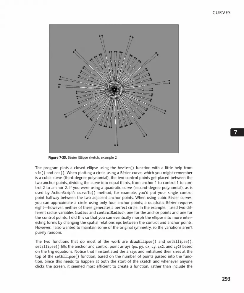
Figure 7-35. Bézier Ellipse sketch, example 2
The program plots a closed ellipse using the bezier() function with a little help fromsin() and cos(). When plotting a circle using a Bézier curve, which you might rememberis a cubic curve (third-degree polynomial), the two control points get placed between thetwo anchor points, dividing the curve into equal thirds, from anchor 1 to control 1 to con-trol 2 to anchor 2. If you were using a quadratic curve (second-degree polynomial), as isused by ActionScript’s curveTo() method, for example, you’d put your single controlpoint halfway between the two adjacent anchor points. When using cubic Bézier curves,you can approximate a circle using only four anchor points; a quadratic Bézier requireseight—however, neither of these generates a perfect circle. In the example, I used two dif-ferent radius variables (radius and controlRadius), one for the anchor points and one forthe control points. I did this so that you can eventually morph the ellipse into more inter-esting forms by changing the spatial relationships between the control and anchor points.However, I also wanted to maintain some of the original symmetry, so the variations aren’tpurely random.
The two functions that do most of the work are drawEllipse() and setEllipse().setEllipse() fills the anchor and control point arrays (px, py, cx, cy, cx2, and cy2) basedon the trig equations. Notice that I instantiated the arrays and initialized their sizes at thetop of the setEllipse() function, based on the number of points passed into the func-tion. Since this needs to happen at both the start of the sketch and whenever anyoneclicks the screen, it seemed most efficient to create a function, rather than include the
CURVES
293
7
617xCH07.qxd 4/17/07 1:38 PM Page 293

same basic code in two different places in the sketch. When a user clicks, setEllipse()is called, passing in a bunch of random values: setEllipse(int(random(3, 36)), random(-200, 300), random(-200, 300));.
The drawEllipse() function is called each frame from the draw() function. You’ll be usingdraw() extensively a little later in the book. draw() is used for animation, and by includingit, Processing continually redraws the screen (by default) around 60 frames per second.You can update values within draw(), as I’m doing by repeatedly calling drawEllipse().Also notice that the first line in the draw() structure is a background(145) call. If I don’tinclude this, the screen will not be cleared between draw loops, and changes to the curveplot will build up on the screen. This could be used to very good effect, so you might wantto try commenting out the background(145) call. Then run the sketch and click the screenrepeatedly. Figure 7-36 shows a screenshot of my attempt.
Figure 7-36. Bézier Ellipse sketch, example 3
PROCESSING: CREATIVE CODING AND COMPUTATIONAL ART
294
617xCH07.qxd 4/17/07 1:38 PM Page 294

I included one last example (shown in Figure 7-37) on how to create an elliptical spline plotusing shape() and shapeVertex(). I also included a more generalized spline ellipse–creation function. Notice how the curveTightness settings affect the different curves,creating interesting path details. Similarly to the bezier() example, I initially populate thecoordinate arrays with ellipse point data, using some trig expressions. However, unlikebezier(), I’m not burdened with anchor and control points. When drawing the closedcurves, I followed the control point order I covered earlier in the chapter. This is not terri-bly intuitive, so it might help to mess with the node order in the curve() functions a littleto see how it affects the curve. I implemented the first ellipse using curve(), and the sec-ond using curveVertex(). I’m not sure which is easier—probably curveVertex(), since ituses a shorter parameter list. The problem with the initial ellipse plots is that they arehard-coded for four points and can’t easily be customized. Thus, I created a more generalspline ellipse function as well, allowing you to control the number of points, as well as thex and y position, radius, and curve tightness, among other properties. The function is usedto generate the two inner curves. This modular approach will be looked at in more depthin the next chapter, as you begin to apply some object-oriented approaches to the examples.
/*Curve EllipseIra Greenberg, December 20, 2005revised November 15, 2006*/
float radius = 165;float angle = 0;
//outer circlefloat[]cx = new float[4];float[]cy = new float[4];
//middle circlefloat[]cx2 = new float[4];float[]cy2 = new float[4];
void setup(){size(400, 400);background(255);strokeWeight(1.5);smooth();
for (int i =0; i<4; i++){//outer ellipsecx[i] = width/2+cos(radians(angle))*radius;cy[i] = height/2+sin(radians(angle))*radius;
//middle ellispecx2[i] = width/2+cos(radians(angle))*(radius*.85);cy2[i] = height/2+sin(radians(angle))*(radius*.85);
CURVES
295
7
617xCH07.qxd 4/17/07 1:38 PM Page 295

angle+=360.0/4.0;}
//outer curvecurveTightness(-3);curve(cx[3], cy[3], cx[0], cy[0], cx[1], cy[1], cx[2], cy[2]);curve(cx[0], cy[0], cx[1], cy[1], cx[2], cy[2], cx[3], cy[3]);curve(cx[1], cy[1], cx[2], cy[2], cx[3], cy[3], cx[0], cy[0]);curve(cx[2], cy[2], cx[3], cy[3], cx[0], cy[0], cx[1], cy[1]);
//middle curvecurveTightness(2);noFill();beginShape();curveVertex(cx2[3], cy2[3]);curveVertex(cx2[0], cy2[0]);curveVertex(cx2[1], cy2[1]);curveVertex(cx2[2], cy2[2]);curveVertex(cx2[3], cy2[3]);curveVertex(cx2[0], cy2[0]);curveVertex(cx2[1], cy2[1]);endShape();
for (int i=0; i<4; i++){fill(255);ellipse(cx[i], cy[i], 10, 10);ellipse(cx2[i], cy2[i], 10, 10);
}
//inner curvecurveEllipse(6, width/2, height/2, radius*.2, -8, 127, true);//inner, inner curvecurveEllipse(8, width/2, height/2, radius*.05, 0, 0, false);
}
// general spline ellipse plotting functionvoid curveEllipse(int pts, int x, int y, float radius, !float tightness, int fillCol, boolean isNodeVisible){float[]cx = new float[pts];float[]cy = new float[pts];float angle = 0;
for (int i=0; i<pts; i++){cx[i] = x+cos(radians(angle))*(radius);cy[i] = y+sin(radians(angle))*(radius);angle+=360.0/pts;
}
PROCESSING: CREATIVE CODING AND COMPUTATIONAL ART
296
617xCH07.qxd 4/17/07 1:38 PM Page 296

curveTightness(tightness);beginShape();fill(fillCol);for (int i=0; i<pts; i++){if (i==0){curveVertex(cx[pts-1], cy[pts-1]);
}curveVertex(cx[i], cy[i]);if (i==pts-1){curveVertex(cx[0], cy[0]);curveVertex(cx[1], cy[1]);
}}endShape(CLOSE);// render control pointsif (isNodeVisible){fill(255);for (int i=0; i<pts; i++){ellipse(cx[i], cy[i], 10, 10);
}}
}
Figure 7-37. Curve Ellipse sketch
CURVES
297
7
617xCH07.qxd 4/17/07 1:38 PM Page 297

The nastiness with the spline curves is in figuring out the order of the control points. It’simportant to remember that each point needs a control point on either side of itself. Inthe block of code for the outer curve:
curve(cx[3], cy[3], cx[0], cy[0], cx[1], cy[1], cx[2], cy[2]);curve(cx[0], cy[0], cx[1], cy[1], cx[2], cy[2], cx[3], cy[3]);curve(cx[1], cy[1], cx[2], cy[2], cx[3], cy[3], cx[0], cy[0]);curve(cx[2], cy[2], cx[3], cy[3], cx[0], cy[0], cx[1], cy[1]);
notice the order of the indices in the array brackets:
3, 0, 1, 20, 1, 2, 31, 2, 3, 02, 3, 0, 1
Each succeeding row begins with the second through the fourth values, and then the nextlogical value is added. Once you get to the highest value (in this case, 3), you go back to 0.I recommend messing with this order to see how it affects the curve.
The curveEllipse() function adds flexibility to the curve-creation process. You generallywant to structure your code to build in as much flexibility as possible. Functions andeventually objects offer this possibility. Notice that the curveVertex() calls in thecurveEllipse() function require some conditional statements within the for loop, ensur-ing that the correct ordering of indices is followed, as discussed earlier:
for (int i=0; i<pts; i++){if (i==0){
curveVertex(cx[pts-1], cy[pts-1]);}curveVertex(cx[i], cy[i]);if (i==pts-1){curveVertex(cx[0], cy[0]);curveVertex(cx[1], cy[1]);
}}
}
Before concluding this chapter, I just want to briefly mention a few more curve-relatedProcessing functions. bezierDetail() and curveDetail() allow you to control the detailof the curve rendering, anywhere from a straight line to a stepped curve to a smooth,flowing curve. However, these functions do not work with the JAVA2D renderer, the cur-rent default rendering mode. You can use them with the P3D and OPENGL renderers,which are covered in Chapters 13 and 14. As of this writing, the P2D renderer is not func-tional. However, if/when that renderer is resurrected, these functions should work with itas well. In addition, there are three other functions—curvePoint(), bezierPoint, andbezierTangent()—that allow points and tangent lines to be plotted along curve paths.These are interesting, but also a little complex, and I think you’ve had enough of that sortof thing in this chapter. More information about these functions can be found inProcessing’s language reference.
PROCESSING: CREATIVE CODING AND COMPUTATIONAL ART
298
617xCH07.qxd 4/17/07 1:38 PM Page 298

SummaryCurves, and the math behind them, offer all sorts of expressive possibilities for creativecoding. They are the basis for generating organic forms and, as you’ll see in Chapter 11,natural motion. Of course, all this power does come with some added complexity. As Iillustrated in this chapter, Processing allows you to generate curves using standard polyno-mial and trigonometric equations. Of course, if the math doesn’t do it for you, you canalso use Processing’s built-in curve functions. As you progress as a coder, though, I thinkyou’ll find the math stuff really helpful—allowing you to more fully exploit the built-infunctions. In Chapter 8, I’ll depart from the math (for a while) and introduce object-oriented programming.
CURVES
299
7
617xCH07.qxd 4/17/07 1:38 PM Page 299

617xCH08.qxd 4/20/07 3:15 PM Page 300

8 OBJECT-ORIENTED PROGRAMMING
617xCH08.qxd 4/20/07 3:15 PM Page 301

Object-oriented programming (OOP) is a deep and complex subject, and a detailed dis-cussion of it is beyond the scope of this book. However, in this chapter I will give you asolid grounding in OOP to get you started. While OOP is challenging to start with, it is fun-damental to Java and therefore Processing, and it is very rewarding once you get the hangof it, so don’t despair if you find this chapter difficult to follow. As you work through therest of the book, it will help you to keep returning to this chapter to look up OOP con-cepts as you meet them in all the applied examples you come across. It will get easier asyou practice, I promise.
A new way of programming?The answer to this question is both yes and no. While very different from procedural pro-gramming, OOP can at the same time be thought of as a natural extension of it. Inprocedural programming, you use functions to modularize code, adding efficiency, organ-ization, and some portability. Classes, the main building blocks of OOP, work similarly.However, OOP takes the modularization of code a couple of magnitudes further. Functionsare like data processing machines. They input data, perform some computation with/onthe data, and spit the data back out to be used somewhere else. Users who utilize a func-tion only need to know what the function does (not how it does it) and what type of datathe function is expecting as input. This type of approach is often referred to as “black-box”design. Electrical components work this way (thankfully). Imagine if you had to understandall the details of how your DVD player works just to watch a film. Instead, you just need toknow how to plug it in and hit play. Functions and classes both provide their own varia-tions on black-box design; they encapsulate their internal implementation while providinga public interface to utilize the structure.
Classes, like functions, are modular, can process data, and allow code to be organized intological structures, adding more organization to the coding process. However, classes gomuch further than functions in their ability to be independent, modular, reusable entities.In addition, classes have built-in variables, called properties, and their own functions,called methods—these properties and methods can be used beyond anything a functioncould provide. In OOP, we say that we interact with a class through its public interface,which can be thought of as the portal to communicate with the class’s black box. Also,unlike functions—which are singular, static processing units—classes provide customizedcopies of themselves called instances, allowing a single class to have a wide range ofunique states or instances. Instances of a class are also referred to as objects, which, if itisn’t obvious, is where the term object-oriented programming comes from.
For example, if I create a Box class, I can then use the class to create Box instances of vary-ing size, shape, color, and so on. Each of the Box instances would share certain core attrib-utes (properties), but these attributes could each be expressed uniquely. Classes can alsoextend other classes. For example, I can create a class called Shape, which I can thenextend to create Rectangle, Circle, and Triangle classes. Each of these three more-specific classes would share certain common attributes, such as position, size, and color,defined within the common Shape class. Aside from the common attributes, instances ofthese classes will also have their own unique characteristics, such as a specific plottingalgorithm, a radius (for a circle), width/height (for a rectangle), an orientation (for a trian-
PROCESSING: CREATIVE CODING AND COMPUTATIONAL ART
302
617xCH08.qxd 4/20/07 3:15 PM Page 302

gle), and so on. These unique attributes would be defined within the specific Rectangle,Circle, and Triangle classes.
The ability for classes to extend other classes is a powerful feature of OOP, allowinglibraries of classes to be developed for reuse. For example, if I create a simple drawingprogram, I could incorporate the existing Rectangle, Circle, and Triangle classes justdiscussed, rather than rebuilding from scratch. Most programming languages come withextensive libraries of classes, greatly simplifying the development process. Processing takesthis concept one step further by creating a procedural front-end (allowing you to simplycall functions) on top of the classes it relies on. The Java language, which you’ll work withtoward the end of the book, is a great example of a mature object-oriented language withthousands of prewritten classes at your disposal.
Now these are a lot of new concepts to absorb without any pictures (or at least code snip-pets), so let’s get to work with some code. Following is an OOP example, based on thecreation (and hopefully consumption) of a Burrito class.
BurritoRecipe classClasses are often used to model specific objects or processes in the real world. I like bur-ritos quite a bit—so let’s make a BurritoRecipe class. Since a class is composed of prop-erties and methods, you need to think about what properties or characteristics a burritorecipe has and what methods or actions would be associated with a burrito recipe. I knowthis sounds very simplistic, but this really is classic object-oriented thinking.
In OOP, you create an abstraction (the class), internally grouping the class’s properties withmethods that act upon these properties, raising program design issues to a higher levelwhere you can think like a person (albeit a hungry person), rather than like a machine. Forexample, once you create your BurritoRecipe class, you could use it by writing somethinglike burritoRecipe1 = new BurritoRecipe(). If you wanted to select pinto beans for yourrecipe, you could then write something like burritoRecipe1.setBeans("pinto"). Classesare often also thought of as blueprints. You use the blueprints to make objects (alsoknown as instances) of the class. For example, the aforementioned burritoRecipe1 is anobject of the BurritoRecipe class. Each object created from a class has access to the samestructure (the class’s internal properties and methods), but each object can also choose toexpress itself differently from other objects derived from the same class. Thus, I can usethe BurritoRecipe class to make a bean burrito recipe, and you can use it to make achicken burrito recipe (or better yet, a chicken and bean burrito recipe).
Here are some BurritoRecipe properties: size, tortillaFlavor, meatType, beanType,toppings, salsaTemperature.
Here are some Burrito methods: getSize(), setSize(), getTortillaFlavor(),setTortillaFlavor(), setMeatType(), getMeatType(), setBeanType(), getBeanType(),getToppings(), setToppings(), setSalsaTemperature(), getSalsaTemperature(), andprintRecipe(). It is the convention, where applicable, to create get and set methods forthe class’s properties. In the preceding list of methods, all of the methods exceptprintRecipe() either get or set properties of the class.
OBJECT-ORIENTED PROGRAMMING
303
8
617xCH08.qxd 4/20/07 3:15 PM Page 303
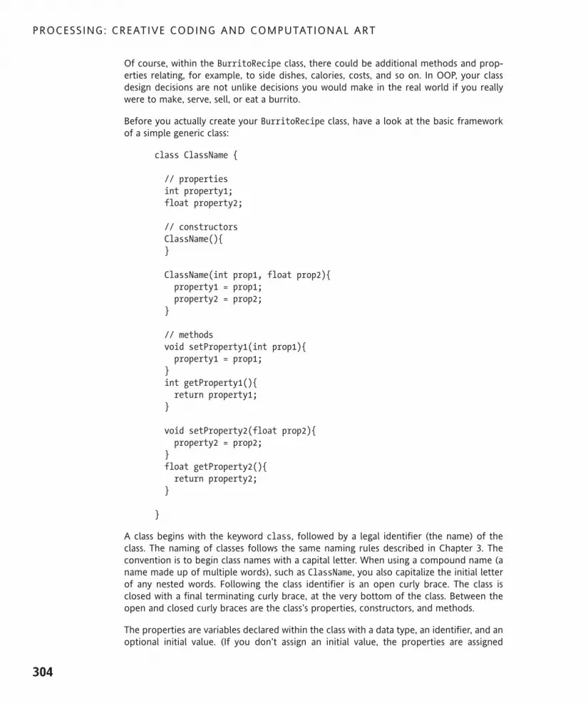
Of course, within the BurritoRecipe class, there could be additional methods and prop-erties relating, for example, to side dishes, calories, costs, and so on. In OOP, your classdesign decisions are not unlike decisions you would make in the real world if you reallywere to make, serve, sell, or eat a burrito.
Before you actually create your BurritoRecipe class, have a look at the basic frameworkof a simple generic class:
class ClassName {
// propertiesint property1;float property2;
// constructorsClassName(){}
ClassName(int prop1, float prop2){property1 = prop1;property2 = prop2;
}
// methodsvoid setProperty1(int prop1){property1 = prop1;
}int getProperty1(){return property1;
}
void setProperty2(float prop2){property2 = prop2;
}float getProperty2(){return property2;
}
}
A class begins with the keyword class, followed by a legal identifier (the name) of theclass. The naming of classes follows the same naming rules described in Chapter 3. Theconvention is to begin class names with a capital letter. When using a compound name (aname made up of multiple words), such as ClassName, you also capitalize the initial letterof any nested words. Following the class identifier is an open curly brace. The class isclosed with a final terminating curly brace, at the very bottom of the class. Between theopen and closed curly braces are the class’s properties, constructors, and methods.
The properties are variables declared within the class with a data type, an identifier, and anoptional initial value. (If you don’t assign an initial value, the properties are assigned
PROCESSING: CREATIVE CODING AND COMPUTATIONAL ART
304
617xCH08.qxd 4/20/07 3:15 PM Page 304

default values based on their specific data type). The properties defined at the top of theclass have global scope within the class, just like variables declared at the top of a sketchin Processing. Variables declared within the head of a constructor or method (parameters),or within the constructor/method blocks, are local to that respective structure. This allworks the same way as functions work in Processing.
The constructors are simply methods (functions declared within a class) with the sameexact name as the class and no specified return type. These special methods are invokedautomatically when an object of the class is created. You can have multiple constructors(each with the same name as the class) as long as the number and type of parameters inthe constructor head (also known as the signature) is different. This also works the sameway as functions work in Processing. Here’s an example of multiple constructors for aShape class. Notice that each constructor has the same name as the class, but a uniqueparameter list. (This code is not intended to be run.)
class Shape{// 1st constructorShape(){}// 2nd constructorShape(float x, float y){}// 3rd constructorShape(float x, float y, float w, float h){}
}
As I mentioned previously, methods are just functions declared within a class. Like func-tions, they can return a value or not, and they can also accept arguments passed intothem. If a method doesn’t return a value, you declare the method using the void keyword.If the method returns a value, you need to declare it with the specific data type it returns.
Now you’re ready to look at a complete class. Please note that the class definition is justone part of the process of using a class. Following my description of the BurritoRecipeclass, I’ll show you how to actually incorporate it into a sketch. The class code is a littlelengthy, but I’ll spend some time going over it.
class BurritoRecipe {
// propertiesint size;String tortillaFlavor;String meatType;String beanType;String[]toppings;int salsaTemperature;
//3 constructors--default, basic, monster//default burrito recipe constructorBurritoRecipe (){}
OBJECT-ORIENTED PROGRAMMING
305
8
617xCH08.qxd 4/20/07 3:15 PM Page 305

//regular burrito recipe constructorBurritoRecipe (String tortillaFlavor, String beanType, !
String meatType){//initialize propertiesthis.tortillaFlavor = tortillaFlavor;this.beanType = beanType;this.meatType = meatType;
}
//monster burrito recipe constructor(uuummmm)BurritoRecipe (String tortillaFlavor, String beanType, !
String meatType, String[]toppings, int salsaTemperature){//initialize propertiesthis.tortillaFlavor = tortillaFlavor;this.beanType = beanType;this.meatType = meatType;this.toppings = toppings;this.salsaTemperature = salsaTemperature;
}
//get/set methodsint getSize() {return this.size;
}
void setSize(int size) {this.size = size;
}
String getTortillaFlavor(){return this.tortillaFlavor;
}
void setTortillaFlavor(String tortillaFlavor){this.tortillaFlavor = tortillaFlavor;
}
String getMeatType(){return this.meatType;
}
void setMeatType(String meatType){this.meatType = meatType;
}
String getBeanType(){return this.beanType;
}
PROCESSING: CREATIVE CODING AND COMPUTATIONAL ART
306
617xCH08.qxd 4/20/07 3:15 PM Page 306

void setBeanType(String beanType){this.beanType = beanType;
}
String[] getToppings(){return this.toppings;
}
void setToppings(String[] toppings){this.toppings = toppings;
}
int getSalsa(int salsaTemperature){return this.salsaTemperature;
}
void setSalsa(int salsaTemperature){this.salsaTemperature = salsaTemperature;
}
void printRecipe(){println("Burrito Recipe:");println("---------------");if (this.tortillaFlavor!=null){println("Steam or lightly pan heat a " + this.tortillaFlavor + !
" tortilla.");if (this.beanType!=null){println("Sauté fresh onions, garlic, cilantro, slowly !
mixing in " + this.beanType + " beans and white wine.");}if (this.meatType!=null){println("Grill " + this.meatType + " along with fresh green !
pepper, jalapeno pepper, chile pepper, !onions and garlic.");
}if (this.toppings!=null){for (int i =0; i< toppings.length; i++){println("Add " + toppings[i]+".");
}}if (this.salsaTemperature>0){println("Finish off with a generous spritz of "+ !this.salsaTemperature+" alarm salsa.");
}}else {println("Uh, you'll need to give me some ingredients\n" + !
"if you actually want me to produce a recipe.");}
OBJECT-ORIENTED PROGRAMMING
307
8
617xCH08.qxd 4/20/07 3:15 PM Page 307

// go to next line after printing// cooking instructions to the screenprintln();
}}
Class declarationclass BurritoRecipe {
As I discussed, to declare a class, you use the class keyword followed by the identifier(BurritoRecipe) of the class. Following the class identifier, there needs to be an opencurly brace.
Properties declaration// propertiesint size;String tortillaFlavor;String meatType;String beanType;String[]toppings;int salsaTemperature;
Properties are declared at the top part of the class. As in previous examples with variables,properties need a data type and a legal identifier to be declared; they can also be assignedinitial values. In this example, I just declare the properties. Notice that of the six proper-ties, two are of type int, three are of type String, and one is of type String[] (array ofStrings). The six declared properties are technically known as instance properties, andeach object created (or instantiated) from the BurritoRecipe class will have access to itsown unique copies of these properties. This is an important point and illustrates the blue-print nature of classes. The properties and methods defined in the class are the core struc-tural elements (commonly referred to as members) of each object instantiated from theclass, and each object can express itself uniquely via its own copies of the class’s proper-ties and methods.
In addition to instance properties, classes can also have static properties and static meth-ods. These are declared with the keyword static. Static properties are also known as classproperties. I will provide an example of some static variables when I cover compositionshortly. The main difference between instance properties and static properties is that eachobject or instance created from a class can assign different values to its instance proper-ties, but all objects of a class share the same values assigned to the class’s static properties.In Java and Processing, static variables are used mostly to create constants (with the addi-tional keyword final added in the declaration). Constants are variables that areimmutable (can’t be changed). For example, in Processing and Java, PI is a constant, andits declaration in Java’s Math package could be something like the following:
static final double PI 3.141592653589793;
PROCESSING: CREATIVE CODING AND COMPUTATIONAL ART
308
617xCH08.qxd 4/20/07 3:15 PM Page 308

Obviously, PI is never going to change, and the complier will enforce this if you use thestatic and final keywords in declaring it. If someone eventually tries to assign someother value to PI, the compiler would generate an error and prevent them from doing it.For the curious among you, the keyword double is the Java data type associated with PI.The double data type is similar to the float type, except a double requires twice as muchstorage as a float (8 bytes vs. 4 bytes), and also has greater precision (accuracy to 15 digits).However, double precision is not really necessary for the types of things most people dowith Processing, so float was made the default primitive data type for any decimal valuesin Processing.
ConstructorsAs mentioned before, constructors are methods with the same name as the class, auto-matically invoked when an object is instantiated (created with the new keyword, as in newBurritoRecipe()). In addition, the constructor returns a reference to the object created.Thus, in the complete instantiation statement
BurritoRecipe myRecipe = new Burrito Recipe();
the variable myRecipe, declared of type BurritioRecipe, is assigned a reference to thenewly created BurritoRecipe object.
//3 constructors--default, basic, monster//default burrito recipe constructorBurritoRecipe (){}
//regular burrito recipe constructorBurritoRecipe (String tortillaFlavor, String beanType, !
String meatType){//initialize propertiesthis.tortillaFlavor = tortillaFlavor;this.beanType = beanType;this.meatType = meatType;
}
//monster burrito recipe constructor(uuummmm)BurritoRecipe (String tortillaFlavor, String beanType, !
String meatType, String[]toppings, !int salsaTemperature){//initialize propertiesthis.tortillaFlavor = tortillaFlavor;this.beanType = beanType;this.meatType = meatType;this.toppings = toppings;this.salsaTemperature = salsaTemperature;
}
OBJECT-ORIENTED PROGRAMMING
309
8
617xCH08.qxd 4/20/07 3:15 PM Page 309

In the BurritoRecipe class, I included three constructors, which allows the class to be ini-tialized three different ways, depending on what arguments are passed to the constructorwhen the object is instantiated. Within the constructors’ parentheses are any optionalparameters. When you create a new object, passing arguments to a constructor, theremust be a constructor with the same number and type of parameters or the compiler willspit out an error, which if you remember is similar to how functions work as well. Thefollowing object instantiations are valid, based on the available constructors in theBurritoRecipe class:
// uses default BurritoRecipe constructorBurritoRecipe recipe1 = new BurritoRecipe();
//uses regular BurritoRecipe constructorBurritoRecipe recipe2 = !
new BurritoRecipe ("spinach", "pinto", "chicken");
However, the following instantiation will generate a compiler error, as there is no con-structor with an appropriate parameter list:
// generates a compiler error.BurritoRecipe recipe3 = new BurritoRecipe ("spinach", "chicken");
Within the code blocks (the code between the curly braces) of the bottom two construc-tors are a number of assignment lines that initialize the class’s instance properties with thevalues passed in via the arguments:
this.tortillaFlavor = tortillaFlavor;this.beanType = beanType;this.meatType = meatType;
These lines may look a little odd at first. I remember being pretty confused when I first sawcode like this. In naming the parameters, I used the same names as the properties declaredat the top of the class. This was technically not necessary, and I could have made thenames different. However, I actually find it easier to remember what parameter valueinitializes what property when they have the same names. Perhaps some of you may bethinking, “When two different things have the same name, couldn’t that create a problem,especially if the properties declared up top have global scope and can be seen anywherewithin the class?” This is a good question. The answer is yes and no. Following, I illustratea good way and a bad way of performing the constructor initialization when both theparameters and the properties have the same names.
Here’s the good code:
this.tortillaFlavor = tortillaFlavor;this.beanType = beanType;this.meatType = meatType;
And here’s the bad code:
tortillaFlavor = tortillaFlavor;beanType = beanType;meatType = meatType;
PROCESSING: CREATIVE CODING AND COMPUTATIONAL ART
310
617xCH08.qxd 4/20/07 3:15 PM Page 310

Hopefully you noticed that the only difference between the good and bad code is theabsence of the this keyword at the beginning of the bad code assignments. If you don’tuse the this keyword, the compiler uses the local parameters on both sides of the assign-ment operator.
The special keyword this refers to the class itself. Thus, this.meatType is the property,not the parameter of the same name. As I mentioned, if you don’t use the keyword this,the compiler will only use the local parameter within the constructor block—so an assign-ment like meatType = meatType doesn’t pass a value to the property, but just uselesslyassigns the parameter value back to the parameter—meaning nothing really happens. Irealize that if this is totally new to you, it may seem like an obscure point, but it really isn’t.Is there any way to avoid using the this keyword? Well, there is, actually. If I had used dis-tinct property and parameter names, I could have avoided using the this keyword. Forexample, the following constructor could be safely substituted for the second constructorin the BurritoRecipe class example:
//basic burrito recipe--add toppings laterBurritoRecipe(String tortFlavor, String bType, String mType){//initialize propertiestortillaFlavor = tortFlavor;beanType = bType;meatType = mType;
}
I still could use the this keyword in front of the properties on the left of the assignmentsif I wanted to, but it is not required any longer. Ultimately, you can do your constructor ini-tializations either way: using the same named properties and parameters and the this key-word in front of the properties, or keeping the property and parameter names distinct. Inmy humble opinion, using the same names for the properties and parameters ultimatelymakes things simpler, and also helps you to see what parameter to assign to what property.But not everyone would agree with me. When you start looking at other people’s code,you’ll see this handled both ways—even though I think I’m right.
MethodsAfter the constructors, there is a long list of methods, in the following style:
int getSize() {return this.size;
}void setSize(int size) {this.size = size;
}
In OOP, there is a convention to structure methods utilizing the get/set prefix appendedto the property names (commonly referred to as get/set methods, or “getters” and“setters”), as illustrated in the preceding code. Not all your methods will be getters andsetters, but generally it is desirable to have a get and set method for each property. In pureOOP (which you’re not totally burdened with here), the idea is that a class’s properties
OBJECT-ORIENTED PROGRAMMING
311
8
617xCH08.qxd 4/20/07 3:15 PM Page 311

should not be targeted directly and the properties should actually be made private, usingthe optional private keyword (called an access modifier) in front of the property declara-tion. For example
private String meatType
If you make the property private, you will not be allowed to directly target it from outsidethe class. Instead, you are forced to use its respective public get/set methods.
So, instead of myBurritoRecipe.meatType = "chicken" or String meat = myBurritoRecipe.meatType;, classic OOP says you must use myBurritoRecipe.setMeatType("chicken"); orString meat = myBurritoRecipe.getMeatType();—I suspect this might be confusing, sofor now, you can go ahead and be naughty and just target your properties directly, whichis actually encouraged in Processing.
In addition to the getter and setter methods, most classes also have additional methodsthat do more interesting things (thank goodness). For example, the printRecipe()method in this program outputs burrito cooking instructions.
void printRecipe(){println("Burrito Recipe:");println("---------------");if (this.tortillaFlavor!=null){println("Steam or lightly pan heat a " + this.tortillaFlavor + !
" tortilla.");if (this.beanType!=null){println("Sauté fresh onions, garlic, cilantro, slowly !
mixing in " + this.beanType + " beans and white wine.");}if (this.meatType!=null){println("Grill " + this.meatType+" along with fresh green !
pepper, jalapeno pepper, chile pepper, onions and garlic.");}if (this.toppings!=null){for (int i =0; i< toppings.length; i++){println("Add " + toppings[i]+".");
}}if (this.salsaTemperature>0){println("Finish off with a generous spritz of " + !this.salsaTemperature+" alarm salsa.");
}}else {println("Uh, you'll need to give me some ingredients\n" + !
"if you actually want me to produce a recipe.");}// go to next line after printing// cooking instructions to the screen
PROCESSING: CREATIVE CODING AND COMPUTATIONAL ART
312
617xCH08.qxd 4/20/07 3:15 PM Page 312

println();}
}
This method may look complex at first glance, but it is really just a bunch of if statementssending output to the text window. One thing that is new in the method is the use of thekeyword null in some of the if statements. For example
if (this.tortillaFlavor!=null){
The conditional expression != means “is not equal to.” So the if statement is then truewhen this.tortillaFlavor is not equal to null. This type of logic can seem tricky whenyou first start using it. Just try to remember that if statements are checking if the condi-tion between the parentheses is true, not for a universal truth. So, if I say ira = tall (I’mnot really), then the conditional if (ira==tall) would evaluate to true, as would if(ira!=short). To explain why I used the null keyword in the first place, I need to go backto the discussion about declaring variables/properties.
Notice that in the class, when I declare a property using the String data type, that Stringhas an initial cap. (Remember that Java and Processing are case sensitive, so the capital Smatters.) Also, throughout the book, when variables of a primitive type have beendeclared—such as int or float—all lowercase letters were used. The capital S in Stringshould inform you that the String data type is a class. Variables or properties declared oftype String, or of any class for that matter, are not primitive types like int, float, orboolean that actually evaluate to specific values, but instead are object reference variablesthat evaluate to the memory address where the objects are stored. Now you don’t need toworry about memory addresses. But what you do need to know is that the default value ofan object reference, once it has been declared and before it has been defined, is null.
In the printRecipe() method, I needed to find a way to keep the program from crashingwhen it couldn’t a find a value it expected. By writing the if statements the way I did, Iensured that if the property was initialized, and therefore wasn’t equal to null, the blockof code would run. However, if it was still equal to null, then the relevant print statementwould be skipped, keeping the program from crashing. This is actually a pretty commonthing to do in coding, and you will see more of it later on in the book.
Throughout the method, I also used the concatenation operator, +, to join the string liter-als in quotes with the properties. Remember, literals are just actual words or numbers thatyou write—for example, “art” (a string literal) or 10 (a number literal, which is referred toas a constant). A literal’s meaning or value is explicitly what is written. To join a literal witha property or variable, you need to use the concatenation operator, as follows:
this.beanType + " beans and white wine."
Also notice within the method that most of the if statements are nested within an outerif statement, which determines if there is a tortilla. If there isn’t a tortilla, then the pro-gram skips the remaining statements and outputs the following:
"Uh, you'll need to give me some ingredients if you actually want meto produce a recipe."
OBJECT-ORIENTED PROGRAMMING
313
8
617xCH08.qxd 4/20/07 3:15 PM Page 313

Alas, if there is no tortilla, there is no way to make a burrito. Lastly, notice how the forloop is used to run through the list of toppings. Using an array for the toppings and thearray’s length property as the limit on the for loop, any number of toppings can be addedto the recipe, and the for loop will automatically loop through the entire array, using thevalue of the array’s length property to determine when to stop. Throughout the rest ofthe book, you’ll see many similar examples using for loops and arrays.
Finally, here’s a complete Processing implementation that actually uses the class. Enter allthe following code into Processing and run the sketch—or better yet, download thecomplete code (BurritoRecipe.pde) from the Download section of the friends of ED site(www.friendsofed.com/).
/*title: BurritoRecipe class exampledescription: create some tasty burritoscreated: August 9, 2005revised: March 10, 2006
October 23, 2006by: Ira Greenbergnote: Enjoy and use plenty of guac.*/
void setup(){// create some burrito recipes//use constructor 1BurritoRecipe b1 = new BurritoRecipe();b1.printRecipe();
//use constructor 2BurritoRecipe b2 = new BurritoRecipe("spinach", "black", "chicken");b2.printRecipe();
//use constructor 3String[]tpgs = {"tomato", "lettuce", "corn"};BurritoRecipe b3 = new BurritoRecipe("whole wheat", "pinto", !
"beef", tpgs , 8);b3.printRecipe();
}
class BurritoRecipe {
// propertiesint size;String tortillaFlavor;String meatType;String beanType;
PROCESSING: CREATIVE CODING AND COMPUTATIONAL ART
314
617xCH08.qxd 4/20/07 3:15 PM Page 314

String[]toppings;int salsaTemperature;
//3 constructors--default, basic, monster//default burrito recipe constructorBurritoRecipe (){}
//regular burrito recipe constructorBurritoRecipe (String tortillaFlavor, String beanType, !
String meatType){//initialize propertiesthis.tortillaFlavor = tortillaFlavor;this.beanType = beanType;this.meatType = meatType;
}
//monster burrito recipe constructor(uuummmm)BurritoRecipe (String tortillaFlavor, String beanType, !
String meatType, String[]toppings, int salsaTemperature){//initialize propertiesthis.tortillaFlavor = tortillaFlavor;this.beanType = beanType;this.meatType = meatType;this.toppings = toppings;this.salsaTemperature = salsaTemperature;
}
//get/set methodsint getSize() {return this.size;
}
void setSize(int size) {this.size = size;
}
String getTortillaFlavor(){return this.tortillaFlavor;
}
void setTortillaFlavor(String tortillaFlavor){this.tortillaFlavor = tortillaFlavor;
}
String getMeatType(){return this.meatType;
}
OBJECT-ORIENTED PROGRAMMING
315
8
617xCH08.qxd 4/20/07 3:15 PM Page 315

void setMeatType(String meatType){this.meatType = meatType;
}
String getBeanType(){return this.beanType;
}
void setBeanType(String beanType){this.beanType = beanType;
}
String[] getToppings(){return this.toppings;
}
void setToppings(String[] toppings){this.toppings = toppings;
}
int getSalsa(int salsaTemperature){return this.salsaTemperature;
}
void setSalsa(int salsaTemperature){this.salsaTemperature = salsaTemperature;
}
void printRecipe(){println("Burrito Recipe:");println("---------------");if (this.tortillaFlavor!=null){println("Steam or lightly pan heat a " + this.tortillaFlavor + !
" tortilla.");if (this.beanType!=null){println("Sauté fresh onions, garlic, cilantro, slowly !
mixing in " + this.beanType + " beans and white wine.");}if (this.meatType!=null){println("Grill " + this.meatType+" along with fresh green !pepper, jalapeno pepper, chile pepper, onions and garlic.");
}if (this.toppings!=null){for (int i =0; i< toppings.length; i++){println("Add " + toppings[i]+".");
}}if (this.salsaTemperature>0){println("Finish off with a generous spritz of " + !
PROCESSING: CREATIVE CODING AND COMPUTATIONAL ART
316
617xCH08.qxd 4/20/07 3:15 PM Page 316

this.salsaTemperature+" alarm salsa.");}
}else {println("Uh, you'll need to give me some ingredients\n" + !
"if you actually want me to produce a recipe.");}// go to next line after printing// cooking instructions to the screenprintln();
}}
There are a couple of ways of using a class in Processing. For one, you can simply add it inyour main tab with the rest of your sketch code, just as you’ve been doing with functions.(To use a custom class or function, you must also include Processing’s setup() function.)You can also enter a class (or function) in a separate tab. The sketch will still see it/treat itas if it exists in the main tab. Finally, you can also work in Java mode, which I’ll cover inChapter 14. For the BurritoRecipe example, I used the simplest solution, and just enteredthe class code directly below the setup() function. At the top of the sketch, withinthe setup() function, I instantiated three BurritoRecipe objects, and called theprintRecipe() method for each of them. When the sketch runs, it outputs burritocooking directions, based on the arguments I passed when I instantiated the threeBurritoRecipe objects.
In the first instantiation statement, I didn’t pass any arguments:
BurritoRecipe b1 = new BurritoRecipe();
The printRecipe() method outputs the following:
Burrito Recipe:---------------Uh, you'll need to give me some ingredientsif you actually want me to produce a recipe.
In the second instantiation statement, I passed three arguments:
BurritoRecipe b2 = new BurritoRecipe ("spinach", "black", "chicken");
The printRecipe() method outputs the following:
Burrito Recipe:---------------Steam or lightly pan heat a spinach tortilla.Sauté fresh onions, garlic, cilantro, slowly mixing in black beans !
and white wine.Grill chicken along with fresh green pepper, jalapeno pepper, !
chile pepper, onions and garlic.
OBJECT-ORIENTED PROGRAMMING
317
8
617xCH08.qxd 4/20/07 3:15 PM Page 317

Finally, when I created the third BurritoRecipe object, I passed in a bunch of stuff:
String[]tpgs = {"tomato", "lettuce", "corn"};BurritoRecipe b3 = new BurritoRecipe("whole wheat", "pinto", !
"beef", tpgs , 8);
The printRecipe() method outputs the following:
Burrito Recipe:---------------Steam or lightly pan heat a whole wheat tortilla.Sauté fresh onions, garlic, cilantro, slowly mixing in pinto beans !
and white wine.Grill beef along with fresh green pepper, jalapeno pepper, !
chile pepper, onions and garlic.Add tomato.Add lettuce.Add corn.Finish off with a generous spritz of 8 alarm salsa.
Hopefully, this example has given you a clear sense of how OOP is implemented inProcessing. However, I don’t think my (albeit very tasty) example properly illustrated thepotential power of OOP. One simple way OOP is useful is in sheer efficiency. It may notseem worth it to generate a whole BurritoRecipe class just to generate a few burritos, butwhat if you needed to generate thousands of different burrito recipes. Clearly, the timespent creating the class begins to pay off big-time. Another way OOP is useful is in organ-izing the coding process. Let’s say I decide to construct an interactive recipe book of 100favorite dishes from around the world, and of course I want to include my burrito recipe.My little BurritoRecipe class included 5 properties and 13 methods, and the other 99world recipes would each contain around the same level of detail. If I don’t use classes, Imight try to code all the hundreds of properties as global and local variables. I’d then needto use lots and lots of functions to sort all this stuff out—pretty much a nightmare sce-nario.
Besides this being a royal pain, I would also lose the connection of each property to itsrespective recipe. Instead, if I use classes, each recipe will enclose, or encapsulate, itsrespective properties and methods, shielding users of the class from much of the internalprocedural complexity and organizing all the hundreds of properties into logical concep-tual structures (classes). Remember, OOP was developed based on the real world and ourbrains’ predilections for thinking of things as discrete units. Going one step further, itwould even be possible to create a RecipeBook class that could encapsulate the individualrecipe objects within the larger organizing class. The bottom line is, as coding problemsget more complex, the benefits gained from OOP begin to far outweigh the costs of imple-menting it.
PROCESSING: CREATIVE CODING AND COMPUTATIONAL ART
318
617xCH08.qxd 4/20/07 3:15 PM Page 318

Advanced OOP conceptsNext, I’ll introduce some advanced OOP concepts, including encapsulation/informationhiding, inheritance, composition, interfaces, and polymorphism. These concepts are fun-damental to OOP, but they’re somewhat difficult to grasp and even harder to effectivelyapply. Understanding these concepts becomes increasingly important as your projectsincrease in size and complexity, especially when you want to create reusable code. Ifyou’re a new coder (and are still recovering from the basic OOP whirlwind tour), youmight want to skip this next section (for now). Just be sure to return to it, as you’ll defi-nitely want to know about this stuff to fully leverage the power of Processing and Java.Fortunately, you can learn these concepts incrementally as you progress as a coder. It’salso possible, if you’re anything like me, that you may end up finding this stuff fascinating.
Encapsulation and data hidingEncapsulation is one of the more “slippery” terms you’ll stumble across when you begin tolearn programming. On the one hand, its meaning in programming is similar to its mean-ing in English—the encasing or enclosing of something. You can think about the way afunction encases lines of code into an invokable unit as a form of encapsulation. One ofthe benefits of this arrangement is that the interface to a function and the implementationwithin the function are separated; this allows the implementation to change over timewhile still maintaining a consistent interface. For example, if I have a function calledcreatePortrait() that initially draws a lousy stick-figure head, over time I can improvethe algorithm to generate a more photorealistic head. The user, then, can just keep callingcreatePortrait() as the interface to the function remains constant, in spite of theimprovements made to the guts of the function.
In OOP, encapsulation refers to the encasing and grouping of an object’s data fields (prop-erties) with its methods. As mentioned earlier, objects are created from classes, each withits own copies of the properties and methods defined in the class. In classic OOP, you don’tgenerally interact with an object’s properties directly. Instead, you use the object’s meth-ods to get or set its property values. This principle is referred to as data or informationhiding. In Java, for example, you normally use the keyword private when declaring prop-erties to make them inaccessible. You declare methods (which are the structures that usersof the class must use to interact with the properties) as public to get and set their values.For example, if I have class that has a name property, I would declare the property as pri-vate like this:
private String name;
And I would create public get and set methods to provide indirect access to the privatename property, as follows:
public String getName (){return name;
}public void setName (String n){name = n;
}
OBJECT-ORIENTED PROGRAMMING
319
8
617xCH08.qxd 4/20/07 3:15 PM Page 319

One of the benefits of data hiding is that dependencies between properties can be bettermanaged. For example, if an object uses the values of a number of properties to calculatesomething, and users are allowed to go in willy-nilly and change any property valuesdirectly, calculations could be adversely affected. However, if you use a method, propertyvalues can be both set and checked prior to performing any calculation, improving uponboth program efficiency and reliability.
All that being said, in Processing, everything is public by default, meaning that to a user ofthe Processing API, everything is directly accessible. This design decision was made to keepProcessing as simple as possible. However, it is possible, especially when working in Javamode, to make your properties private and enforce data hiding. In Chapter 14, you’ll workin Java mode, making your object properties private and using public get and set methodsto interact with them. To learn more about this concept, check out http://java.sun.com/docs/books/tutorial/java/concepts/object.html.
InheritanceInheritance in OOP is the ability of a class A to inherit or extend another class, B, enablingclass A to have access to the properties and methods within the extended class B. In thisconstructed relationship, class B is referred to as the superclass that class A extends, andclass A becomes the subclass that extends class B. In addition, class A can add its own addi-tional properties and methods, and even overwrite specific properties and methods ofclass B (its extended superclass). Inheritance proceeds in a general-to-specific direction.For example, if I have a class called GermanShepherd, I could start with a very general baseclass, called Mammal, a subclass of Mammal called Quadruped, a subclass of Quadruped calledCanine, and a subclass of Canine called GermanShepherd. A Feline class could also inheritfrom Quadruped, while a Human class might come from a Biped class that inherited fromMammal. Figure 8-1 shows a diagram of this.
Figure 8-1. OOP inheritance diagram
PROCESSING: CREATIVE CODING AND COMPUTATIONAL ART
320
617xCH08.qxd 4/20/07 3:15 PM Page 320

Inheritance in Java is absolutely fundamental to the language’s design. In fact, every classin Java except the Object class has at a minimum one superclass, and every class exceptthe Object class has a lineage that goes back to Object. For example, when you export aProcessing sketch, a Java applet is created. Here is the Applet class’s lineage:
java.lang.Objectjava.awt.Component
java.awt.Containerjava.awt.Panel
java.applet.Applet
The classes are the words that start with an initial cap (Object, Component, Container,Panel, and Applet). The words connected to them by a dot are the packages the classeslive in. Packages are just directories or folders that hold class files. In this lineage, Appletinherits from Panel, which inherits from Container, which inherits from Component, whichinherits from Object. Therefore, the Applet class has access to all the accessible proper-ties and methods declared within its own class and from all the classes above it—giving theApplet class access to over 200 methods. However, the inheritance chain doesn’t go theother way. Object doesn’t have access to any properties or methods besides thosedeclared within its own class description, as it is at the top of the inheritance chain for allclasses. On the other hand, the Panel class has access to methods/properties inContainer, Component, and Object—but not Applet.
Applying inheritanceUsing inheritance is pretty straightforward. In the following example, I have a very simpleShape class and Polygon class. The Polygon class inherits from (or extends) the Shape class.
class Shape {//class propertiesint x;int y;int w;int h;
//constructorsShape (){}
Shape (int x, int y, int w, int h){this.x = x;this.y = y;this.w = w;this.h = h;
}}
class Polygon extends Shape{int pts;//constructor
OBJECT-ORIENTED PROGRAMMING
321
8
617xCH08.qxd 4/20/07 3:15 PM Page 321
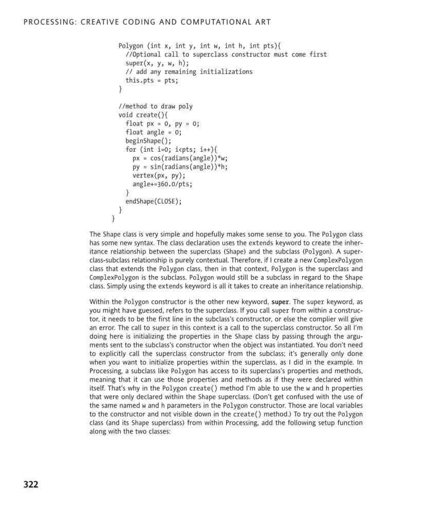
Polygon (int x, int y, int w, int h, int pts){//Optional call to superclass constructor must come firstsuper(x, y, w, h);// add any remaining initializationsthis.pts = pts;
}
//method to draw polyvoid create(){float px = 0, py = 0;float angle = 0;beginShape();for (int i=0; i<pts; i++){px = cos(radians(angle))*w;py = sin(radians(angle))*h;vertex(px, py);angle+=360.0/pts;
}endShape(CLOSE);
}}
The Shape class is very simple and hopefully makes some sense to you. The Polygon classhas some new syntax. The class declaration uses the extends keyword to create the inher-itance relationship between the superclass (Shape) and the subclass (Polygon). A super-class-subclass relationship is purely contextual. Therefore, if I create a new ComplexPolygonclass that extends the Polygon class, then in that context, Polygon is the superclass andComplexPolygon is the subclass. Polygon would still be a subclass in regard to the Shapeclass. Simply using the extends keyword is all it takes to create an inheritance relationship.
Within the Polygon constructor is the other new keyword, super. The super keyword, asyou might have guessed, refers to the superclass. If you call super from within a construc-tor, it needs to be the first line in the subclass’s constructor, or else the complier will givean error. The call to super in this context is a call to the superclass constructor. So all I’mdoing here is initializing the properties in the Shape class by passing through the argu-ments sent to the subclass’s constructor when the object was instantiated. You don’t needto explicitly call the superclass constructor from the subclass; it’s generally only donewhen you want to initialize properties within the superclass, as I did in the example. InProcessing, a subclass like Polygon has access to its superclass’s properties and methods,meaning that it can use those properties and methods as if they were declared withinitself. That’s why in the Polygon create() method I’m able to use the w and h propertiesthat were only declared within the Shape superclass. (Don’t get confused with the use ofthe same named w and h parameters in the Polygon constructor. Those are local variablesto the constructor and not visible down in the create() method.) To try out the Polygonclass (and its Shape superclass) from within Processing, add the following setup functionalong with the two classes:
PROCESSING: CREATIVE CODING AND COMPUTATIONAL ART
322
617xCH08.qxd 4/20/07 3:15 PM Page 322

void setup(){size(400, 400);background(50);smooth();Polygon p = new Polygon(0, 0, 175, 175, 8);translate(width/2, height/2);p.create();
}
One final point: Processing and Java allow a superclass to be assigned an object referenceto any class that has extended it or is below it in the inheritance lineage. Thus, an object ofthe Object class can be assigned an object reference to any class, because the Object classsits alone at the very top of the entire class lineage. So it is perfectly legal and common towrite a statement like this:
Shape myShape = new Polygon(10, 19, 233, 100, 8);
Inheritance gives Processing and Java a lot of power, efficiency, and flexibility. Applying itjudiciously, however, is not always so simple. One of the potential problems with inheri-tance is that classes get locked into dependencies. So, if I eventually decide to change aclass for reuse, I may inadvertently mess up another program that depends, through inher-itance, on a certain implementation within a superclass. This scenario and how to deal withit is a pretty advanced and subtle concern that won’t apply to most new coders, but it issomething to keep in the back of your mind as you begin to develop larger and morecomplex projects.
CompositionOne alternative (and also complimentary) approach to inheritance is called composition.Composition is another technique for developing relationships between classes. Compositionis pretty straightforward to implement, and I think easier to get your head around thaninheritance. Let’s imagine I’m trying to develop a virtual house. My house will be reallysimple; it will only contain windows. The windows, however, are pretty fancy. In OOP, it isvirtuous to be able to modularize a construct into a class, encapsulating its properties andbehavior. Thus, it would be a good idea to create a Window class and have the class inter-nally take care of creating and customizing the windows. Then, in my House class, I couldjust worry about where the windows are going to go and maybe how big to scale them; theWindow class would take care of everything else. This is good OOP design. However, thisapproach also involves having multiple classes interacting with one other. The challenge ofthis inter-class communication is that unless there is an inheritance relationship, an objectfrom one class can’t effectively communicate with an object of an unrelated class. In myprevious inheritance example, the Polygon class extended the Shape class. This madesense because a polygon is a type of shape. Can I do the same thing with the House andWindow? Not really, as a window is not a type of house. Thus inheritance doesn’t concep-tually seem like the right choice.
OBJECT-ORIENTED PROGRAMMING
323
8
617xCH08.qxd 4/20/07 3:15 PM Page 323

Composition can solve this problem elegantly. Although I can’t say that a window is a typeof house, I can say that a house has a window. This is the difference between inheritanceand composition. Inheritance involves an is-a relationship and composition involves a has-a relationship. Which approach would work with the following class groupings?
Mammal, Cat
Artist, CreativeCoder
Monkey, Tail
Foot, Finger
EatingTool, Spoon, Fork
Well, a cat is a mammal, and a creative coder is an artist—these are both examples ofinheritance. A monkey has a tail, which is an example of composition. A foot, however,doesn’t have a finger; nor is a finger a type of foot—so neither relationship makes sense—this is an annoying tricky one. Lastly, a spoon and a fork are both eating tools, which isanother example of inheritance.
Following is some class code illustrating how to apply the composition relationship.
class Window {/* declare static properties: the final keyword ensures
that these constant values can't be changed. */static final int RECTANGLUAR = 1;static final int ELLIPTICAL = 2;static final int OCTAGONAL = 3;
// instance propertiesint panes;boolean isDoublePaned;int configuration;
// constructorWindow (int panes, boolean isDoublePaned, int configuration){this.panes = panes;this.isDoublePaned = isDoublePaned;this.configuration = configuration;
}// other Window methods would go here
}
class House {// instance properties
/* The House class contains a property of type Window */
Window win;
// constructor/* The House constructor expects
PROCESSING: CREATIVE CODING AND COMPUTATIONAL ART
324
617xCH08.qxd 4/20/07 3:15 PM Page 324
a Window object argument */House(Window win){this.win = win;
}// other House methods would go here}
From within Processing, I could use these classes like this (assuming, of course, that thetwo classes were pasted below the setup() function, or each in their own separate tab):
void setup(){Window myWin = new Window(4, true, Window.ELLIPTICAL);House myHouse = new House(myWin);
}
Notice that I included three constants in the Window class. It is a coding convention to useall caps for constant names. One of the most common uses for constants is for presetvalues. In my example, I am giving a user of the Window class a choice of three differentwindow configurations. I could have just forced the user to type in a number, but it is eas-ier for most people to remember a name. In my Window class, I would eventually want toadd a method that figures out what constant the user selected (which is just an int value),and then have that type of window created. You’ll notice in the Processing setup() func-tion that I use the static ELLIPTICAL property by attaching it to the class name with a dot(Window.ELLIPTICAL). Static properties are class properties that are accessible from anyclass. There is no need to instantiate an object of the class to use them. Remember alsothat Processing and Java are case sensitive, so when using the class name, you need the ini-tial capital.
After the static properties, I declare three instance properties, which should hopefully lookfamiliar by now. Next, in the Window constructor, I do my normal parameter-to-propertyassignments. I didn’t include any other methods in the class for the sake of brevity (as ifthat were still possible).
The House class is very short, but gives a clear example of class composition. I onlydeclared one instance variable, and you’ll notice it is of type Window. Now this may lookpretty odd, as you normally declare a property or variable as a valid data type, built intothe Processing and Java core languages. Well, it so happens that any class you create is avalid data type. The subtlety of this concept took me some time to fully grasp. Just remem-ber that a class is a data type. So it is perfectly valid to declare a property of a class type.
In the House constructor, there is a parameter of type Window that requires that an argu-ment of type Window be passed in when a House object is instantiated. Within the Houseconstructor, I do a standard assignment, using the parameter and property—both of typeWindow. The really cool thing is that now I can communicate directly with the Windowobject from within the House class, through its internal reference passed into the Houseconstructor. Of course, if I were to finish the class, I would want to include additionalproperties and methods, allowing the Window object to be placed and sized within thehouse.
OBJECT-ORIENTED PROGRAMMING
325
8
617xCH08.qxd 4/20/07 3:15 PM Page 325

There are many advantages for House and Window to have this special compositional rela-tionship. By letting the house control when and where to draw the windows, it can ensurethat the windows always fit, regardless of whether the house is resized or moved. By let-ting the windows take care of actually drawing themselves, the house only has to worryabout the number of windows, their scale, and where they go. This is good, clean OOP inaction.
I realize that this is not easy stuff to grasp in its entirety, but I hope you are getting a senseof what OOP is and why it might be useful. The best way to learn OOP is to practice andexperiment writing classes/programs. You can read this stuff over and over, but until youapply it, it’s hard to get it to stick. The final concepts we’ll look at in this long chapter arenot easy, so read at your own risk. If you choose to jump ahead, which is fine, do try tocome back at some point.
InterfacesIn the example on inheritance a couple of pages back, a Polygon class extended a Shapeclass. This allowed the Polygon class to access the class members of the Shape class. Thismade sense because of the is-a relationship. A polygon is a shape. In the compositionexample, the House class contained a reference to the Window class through an instancevariable of type Window. This was the right solution because a house has a window, but awindow is not a house. I could have also used the Shape class as a base class for both theHouse and Window classes, as both a window and a house are shapes (of a sort). It is possi-ble and actually very common to combine inheritance and composition when designingclasses.
However, there are times when you’ll have a class that has an is-a relationship to two ormore classes. For example, a Bicycle class could have an is-a relationship to a Vehicleclass and also a SportsGear class. Since the SportsGear class and the Vehicle class don’thave much in common, you can’t logically create an inheritance chain, where the Bicycleclass extends the SportsGear class that extends the Vehicle class. The most logical solu-tion is one of multiple inheritance, where the Bicycle class extends both the Vehicle classand the SportsGear class. In a language like C++, this could be done. However, in Java andProcessing, this is illegal, as the languages don’t support multiple class inheritance, whichmany people think is a good thing. If you want to learn more about this issue, check outwww.javaworld.com/jw-12-1998/jw-12-techniques.html. However, Java/Processing doessupport another approach to multiple inheritance, often referred to as multiple inheri-tance of interface.
Interfaces are class-like constructs that can only include method definitions and constants.Interfaces can’t include method implementations, the stuff between the curly braces.Method definitions include a return type (or the keyword void), the identifier (name) ofthe method, and the number and type of parameters. For example, method definitions ina SportsGear interface might include the following:
String getBrandName();float getUnitCost();void setUnitCost(float unitCost);void printWarranty();
PROCESSING: CREATIVE CODING AND COMPUTATIONAL ART
326
617xCH08.qxd 4/20/07 3:15 PM Page 326

The entire SportsGear interface in Processing would be:
interface SportsGear{String getBrandName();float getUnitCost();void setUnitCost(float unitCost);void printWarranty();
}
It’s pretty simple to create interfaces. However, using them is a bit trickier, and using thempolymorphically is trickier still. We’ll take it one step at a time. Here’s a Bicycle class thatextends a Vehicle class and implements the SportsGear interface (this code is not meantto be run):
class Bicycle extends Vehicle implements SportsGear{//instance variablesString brandName;float unitCost;
// constructorBicycle(String brandName, float unitCost){this.brandName = brandName;this.unitCost = unitCost;
}
/* We're required to implement all methodsfrom the SportsGear interface*/
String getBrandName(){return brandName;
}float getUnitCost(){return unitCost;
}void setUnitCost(float unitCost){this.unitCost = unitCost;
}void printWarranty(){println("Bicycle: full replacement value for 1 year");
}}
To keep things simple in the example, I didn’t bother adding any properties or methods tothe Vehicle class, or extra properties/methods to the Bicycle class. Instead, the Bicycleclass gets all of its members just by implementing the SportsGear interface. Whenever aclass implements an interface—through the use of the implements keyword—the classmust implement all the methods in the interface, which means that it needs to include allthe method definitions contained within the interface, as well as fill in the method blocks.This is enforced by the compiler, which will generate an error if it’s not done.
OBJECT-ORIENTED PROGRAMMING
327
8
617xCH08.qxd 4/20/07 3:15 PM Page 327

When I first learned about interfaces, by about this point in the discussion I got kind ofannoyed. I was able to follow how to code interfaces, but I didn’t get the benefit. I mean,if you are forced to implement all the methods in the interface, why not just add themethods directly to the class to begin with? Wouldn’t this be less work and less confusing?What is the interface really giving you for this added effort? I think in retrospect that thiswas a good question. At this point, there is not much apparent benefit.
Let’s now create another class that also implements the SportsGear interface, to see if youcan begin to see the power of interfaces. (This code is not intended to be run either—I’llget to that shortly.)
class Skis implements SportsGear{//instance variablesString brandName;float unitCost;
// constructorSkis(String brandName, float unitCost){this.brandName = brandName;this.unitCost = unitCost;
}// required implemented interface methodsString getBrandName(){return brandName;
}float getUnitCost(){return unitCost;
}void setUnitCost(float unitCost){this.unitCost = unitCost;
}void printWarranty(){
println("Skis: full replacement value for 5 years");}
}
In the Skis class, you can see that I included the same method definitions as in theBicycle class. Notice also that I implemented the printWarranty() method a little differ-ently in each of the two classes. I have the freedom to do this because the interfacemethods are empty. This is one of the benefits of using interfaces. They provide a sharedinterface for communicating with a group of related classes, but still allow a customizedimplementation of each of the common methods. As you get more experienced withcoding, you’ll begin to recognize some recurring patterns in how related classes aredesigned, and even eventually be able to guess at some of the classes’ methods
The customized implementation benefit I just mentioned is helpful, but still for my money,not quite enough to add so much complexity or extra work to my process. However,before you write off interfaces, there is another much more powerful benefit to usingthem that justifies the extra effort—polymorphism.
PROCESSING: CREATIVE CODING AND COMPUTATIONAL ART
328
617xCH08.qxd 4/20/07 3:15 PM Page 328

PolymorphismPolymorphism sounds a lot worse than it really it is; it just means assuming multiple formsor shapes. Whether you realize it or not, you’re already very familiar with how polymor-phism works. For example, imagine you and a friend decide to spend one Sunday buildinga birdhouse. You’d probably want some tools—say, a screwdriver and a saw. These toolsdon’t have much in common with one another except their general classification as tools.In OOP speak, we could say that each tool has two types: the type Tool and also its morespecific type (Screwdriver or Saw). As you’re building the birdhouse, your friend is hold-ing a screw and asks you to pass him a tool. Unless you’re a prankster, you pass him thescrewdriver. Even though your friend didn’t specify which tool; the context determinedwhich was appropriate. Also, since both the screwdriver and the saw are tools, there wasno risk (when he asked for a tool) of you passing him a ham sandwich or whatever. Thisdynamic binding between a more general classification (tool) and a specific object (screw-driver), based on context, is precisely how polymorphism works in OOP.
In technical terms, polymorphism in Processing/Java is based on the JVM’s ability to beable to link a method to a specific class’s implementation on the fly, making it possible fora well-designed program to actually expand and grow over time, without necessarily goingback into the source code. For example, let’s say you created a video game that includedcreatures who could each cast different magical spells. Using polymorphism, it would bepossible to code a system that could handle any number of creatures, including new onesyou added after the main game engine was complete—without ever having to go backinto the engine’s source code. Here’s a very simple code example of this scenario that youcan run in Processing:
// polymorphism example using inheritancevoid setup(){Creature c = new Creature();Ogre o = new Ogre();Elf e = new Elf();Engine eng = new Engine();eng.addCreature(c);eng.addCreature(o);eng.addCreature(e);
}
//superclassclass Creature{void castSpell(){println("nothing to say");
}}
//subclass 1class Ogre extends Creature{void castSpell(){println("I miss ya donkey");
}}
OBJECT-ORIENTED PROGRAMMING
329
8
617xCH08.qxd 4/20/07 3:15 PM Page 329
//subclass 2class Elf extends Creature{void castSpell(){println("Gotta make the cookies");
}}
/* game engine--with embedded superclassreference in the addCreature() method */class Engine{void addCreature(Creature c){c.castSpell();
}}
In the example, the Ogre and Elf classes each extend the Creature class. Through thisinheritance relationship, any Ogre and Elf objects instantiated will now also be of the sec-ondary type Creature. Thus, it would be perfectly legal to assign new Ogre and Elf objectsto variables declared of type Creature.
Creature o = new Ogre();Creature e = new Elf();
However, as you continue to expand this example, you’ll want the Ogre and Elf objects tobe assigned to variables of type Ogre and Elf, respectively—so if you tried using the pre-ceding superclass assignment lines (which would work for now), make sure you put themback to what they were:
Ogre o = new Ogre();Elf e = new Elf();
This capability of unrelated objects (created from different classes) to have a relationshipthrough a common parent class (which each class extends) allows you to create more-flexible programs. For example, if you create a game that includes the Ogre and Elf crea-tures, inside the game engine you’d either have to hard-code reference variables for eachof the creatures, or use a common extended class. For only two creatures, either optionmight be fine. However, what if your game included 20 creatures, or even the capabilityfor players to create their own creatures? The last thing you’d want to do is to keep goinginto your game engine code and adding new reference variables every time a player cre-ated a new creature. Rather, by including a common superclass reference variable in yourengine, you could simply require players creating a new creature class to extend your baseCreature superclass. This would allow your game to scale up, without you’re ever havingto touch the game engine source code.
Besides including a reference to the superclass in your game engine, you’d also need com-mon methods within the Creature superclass and all the individual subclasses. In my lastexample, notice the common castSpell() method within the Creature superclass andboth the Ogre and Elf subclasses. These methods have identical signatures (same nameand parameter list). However, their implementations (the code between the curly bracesof the methods) are different. As I mentioned earlier, one of the benefits of inheritance is
PROCESSING: CREATIVE CODING AND COMPUTATIONAL ART
330
617xCH08.qxd 4/20/07 3:15 PM Page 330

that a subclass has access to the superclass’s methods (and properties). It’s also possiblefor a subclass to override methods within the superclass. This is accomplished by creatingmethods in the subclass with identical signatures to methods in its superclass.
In the last example, the following three instantiation lines
Creature c = new Creature();Ogre o = new Ogre();Elf e = new Elf();
create Creature, Ogre, and Elf objects (the Ogre and Elf objects are also of typeCreature, through inheritance). The addCreature(Creature c) method in the Engineclass includes a parameter of type Creature, allowing not only objects of type Creature tobe passed to the method as arguments, but also any subclasses of Creature. Inside thismethod is a call, using the passed-in object reference, to the common castSpell()method. Here’s where the magic happens. In setup(), when I call the EngineaddCreature() method three times:
eng.addCreature(c);eng.addCreature(o);eng.addCreature(e);
passing in Creature, Ogre, and Elf objects, respectively, the JVM automatically figures outwhich implementation of the castSpell() method to call, based on the passed-in argu-ment. In the first call, I’m passing in an object of type Creature, so the castSpell() imple-mentation in the superclass is used. But in the next two calls, the castSpell()implementations within the Ogre and Elf subclasses, respectively, are used. This is poly-morphism in action and a powerful feature of Processing and Java.
Polymorphism with interfaces
Another variation on polymorphism in Java/Processing involves the use of interfaces. As Imentioned earlier, classes are data types, and a class that extends another class becomesof that secondary type as well. Interfaces are also legal data types—you can declare anobject reference variable as an interface type, just like a class type. In the SportsGearinterface discussion a few pages back, the Bicycle and Skis classes each implemented theSportsGear interface. Thus, instantiated Bicycle and/or Skis objects would also both beof the secondary type SportsGear. The Bicycle class also extended a Vehicle class, so itwould actually be of three types: Bicycle, Vehicle, and SportsGear. In Processing andJava, a class is only allowed to extend a single class, but it can implement as many inter-faces as you’d like. This is why it is said that multiple inheritance of interface is permittedin Processing/Java.
At the risk of scaring readers away from the last few pages of this chapter, Ifeel it’s only fair to warn you that you’re about to head down a double blackdiamond trail (of the mind). This material is very advanced and presented ina condensed format. Read it at your own risk.
OBJECT-ORIENTED PROGRAMMING
331
8
617xCH08.qxd 4/20/07 3:15 PM Page 331

Returning to the creature engine example, let’s say some of the creatures have archerycapabilities. It would be possible to add archery capabilities directly within the Creatureclass (which each class extends), but of course not all creatures would be archers, so itreally doesn’t belong in the Creature superclass. Another possible option might be tocreate a new Archer class, but the problem there is that you’re not allowed to have a classin Processing/Java extend more than one class. Since each creature needs to extend theCreature class, it wouldn’t be possible to also extend the Archer class. Using an interfacecan help solve this problem. As discussed, an interface can only include constants andunimplemented methods (method signatures). Here’s a very simple Archer interface:
interface Archer{void shoot();
}
This interface only includes a shoot() method; notice the absence of curly braces follow-ing the shoot() method signature. To use the interface, you need to add the implementskeyword along with the interface name to the end of another class declaration. I’ll add theinterface to the Elf class and also to a new Knight class. Here’s what the class declarationstatements look like:
class Elf extends Creature implements Archerclass Knight extends Creature implements Archer
And here are the completed Elf and Knight classes:
// Elf classclass Elf extends Creature implements Archer{void castSpell(){println("Gotta make the cookies");
}
// required method from interfacevoid shoot(){println("Elf shoots");
}}
//Knight classclass Knight extends Creature implements Archer{void castSpell(){println("Mirror, mirror on thw wall...");
}// required method from interfacevoid shoot(){println("Knight shoots");
}}
Notice that both classes contain the shoot() method, including their own unique imple-mentations. It’s important to remember that any class that implements an interface is
PROCESSING: CREATIVE CODING AND COMPUTATIONAL ART
332
617xCH08.qxd 4/20/07 3:15 PM Page 332

forced to literally implement the interface—meaning add curly braces and fill in the bodyof the method. Next, I’ll add a launchArrow(Archer a) method to the Engine class, whichincludes a parameter of the Archer interface type. Here’s the completed Engine class:
class Engine{void addCreature(Creature c){c.castSpell();
}void launchArrow(Archer a){a.shoot();
}}
The launchArrow() method works the same way as the addCreature() method. When thelaunchArrow() method is called, the respective shoot() method implementation (in aclass implementing the Archer interface) will be selected based on what specific type themore general Archer types evaluate to. Finally, here’s the updated setup() function,including the new Knight instantiation and launchArrow() method calls:
void setup(){Creature c = new Creature();Ogre o = new Ogre();Elf e = new Elf();Knight k = new Knight();Engine eng = new Engine();
eng.addCreature(c);eng.addCreature(o);eng.addCreature(e);
eng.launchArrow(e);eng.launchArrow(k);
}
I want to make one final modification to this example. In the setup() function, I originallyinstantiated the Creature object only to help illustrate how method implementations canbe dynamically selected, based on the type of the passed argument. When I passed in asubclass object, its castSpell() implementation was used, but when I passed in the super-class object, the castSpell() implementation within the superclass was actually used. Inreality, you generally wouldn’t want to instantiate a Creature object. Instead, you’re onlyinterested in using the Creature class as a base for more specific creatures.
Java includes the reserved keyword abstract, which can be used to enforce this behavior.You simply preface the class declaration with the abstract keyword, turning the class intoan abstract class. Here’s the Creature class as an abstract class:
abstract class Creature{void castSpell(){println("nothing to say");
}}
OBJECT-ORIENTED PROGRAMMING
333
8
617xCH08.qxd 4/20/07 3:15 PM Page 333

Once a class is declared abstract, the complier will not allow it to be instantiated. So, in thelast example, if I add the abstract keyword in front of the Creature class, I’ll get an errorwhen I try to run the sketch. However, if I remove the Creature instantiation line as well asthe line below it, where the engine adds the Creature object c, the sketch will run fine.Besides enforcing this behavior, abstract classes also allow you to add abstract methods tothe class. Abstract methods are simply method declarations (like in interfaces) that alsorequire the abstract keyword. Here’s an example:
abstract String getCreatureName();
Also similar to interfaces, any class that extends an abstract class must implement allabstract methods within the superclass. However, unlike interfaces, abstract classes alsoallow you to include concrete methods (regular implemented methods) within the class. Itis not necessary for a subclass to reimplement the abstract superclass’s concrete methods,but of course, as in the example, it can override them. Here’s the completed polymor-phism example, including the Archer interface and abstract Creature superclass. I alsoadded an abstract getCreatureName() method to the Creature superclass, which I thenimplemented in each of the (concrete) subclasses.
/* polymorphism example usinginheritance, interface andan abstract class */void setup(){Ogre o = new Ogre();Elf e = new Elf();Knight k = new Knight();Engine eng = new Engine();
eng.addCreature(o);eng.addCreature(e);
eng.launchArrow(e);eng.launchArrow(k);
println(o.getCreatureName());println(e.getCreatureName());println(k.getCreatureName());
}
// abstract Creature superclassabstract class Creature{/* this method will be overriden byCreature subclasses */void castSpell(){println("nothing to say");
}
//abstract getCreatureName methodabstract String getCreatureName();
}
PROCESSING: CREATIVE CODING AND COMPUTATIONAL ART
334
617xCH08.qxd 4/20/07 3:15 PM Page 334

// Ogre subclassclass Ogre extends Creature{// overriden method within Creature superclassvoid castSpell(){println("I miss ya donkey");
}
/* required method implementationfrom abstract Creature superclass */String getCreatureName(){return "I am an an Ogre";
}}
// Elf subclassclass Elf extends Creature implements Archer{// overriden method within Creature superclassvoid castSpell(){println("Gotta make the cookies");
}
/* required method implementationfrom interface Archer */void shoot(){println("Elf shoots");
}
/* required method implementationfrom abstract Creature superclass */String getCreatureName(){return "I am an an Elf";
}}
// Knight subclassclass Knight extends Creature implements Archer{// overriden method within Creature superclassvoid castSpell(){println("Mirror, mirror on thw wall...");
}
/* required method implementationfrom interface Archer */void shoot(){println("Knight shoots");
}
OBJECT-ORIENTED PROGRAMMING
335
8
617xCH08.qxd 4/20/07 3:15 PM Page 335

/* required method implementationfrom abstract Creature superclass */String getCreatureName(){return "I am a Knight";
}}
interface Archer{void shoot();
}
/* game engine-with embedded superclassreference in the addCreature() methodand embedded interface reference inlaunchArrow method */class Engine{void addCreature(Creature c){c.castSpell();
}void launchArrow(Archer a){a.shoot();
}}
Sorry if the text output is anticlimactic. Later on in the book, you’ll use OOP and polymor-phism to generate some interesting visuals. In this chapter, we needed to get some theoryout of the way—which we’ve now done.
SummaryThis was not an easy chapter. OOP introduces many abstract concepts to an alreadyabstract activity—programming. However, as you begin to create more complex sketches,the organizational and reusability benefits of OOP make it well worth the added complex-ity. Also, like any craft-based pursuit, the process gets easier through practice. The firstpart of the chapter dealt with the basics of OOP—classes and objects. I think you’ll findworking with simple classes in Processing straightforward and helpful. For example, whencreating an animation, it’s helpful to encapsulate the animated object’s properties (e.g., x,y, width, and height) inside a class, allowing you to target the properties using dot syntax(e.g., animatedObject.x). In the advanced OOP section, you looked at some pretty com-plex concepts, including inheritance, interfaces, abstract classes, and polymorphism.Understanding and implementing these concepts takes time. Fortunately, you can do a lotwithout them. However, as you build ever more complex sketches, these advanced fea-tures can provide much greater flexibility and efficiency to your sketch design. You’ll beusing most of the features discussed in this chapter throughout the book (to accomplishmore interesting things than getting some text output).
PROCESSING: CREATIVE CODING AND COMPUTATIONAL ART
336
617xCH08.qxd 4/20/07 3:15 PM Page 336

617xCH08.qxd 4/20/07 3:15 PM Page 337

617xCH09.qxd 4/18/07 3:38 PM Page 338

9 SHAPES
617xCH09.qxd 4/18/07 3:38 PM Page 339

Shapes are a natural extension of lines and curves. In the simplest sense, a shape is just theenclosed space formed between three or more lines. Of course, a single continuous curvecan enclose space as well (e.g., an ellipse). Shapes can be generally categorized. For exam-ple, an enclosed three-sided shape is referred to as a triangle, even if its size or configura-tion can’t be determined. Fundamental 2D shapes (e.g., rectangles, circles, and triangles)are commonly referred to as primitives. Primitives are essential building-block shapes,which when combined allow you to (efficiently) construct most other shapes. Processingincludes both 2D and 3D primitive functions. In this chapter, you’ll just be dealing with 2Dshape functions.
I’ll begin by creating some simple sketches based on Processing’s primitive 2D shape func-tions. These sketches will also provide a quick review of some of the core conceptscovered in earlier chapters. Using Processing’s drawing commands, I’ll then show you howto create your own custom shapes, and eventually you’ll work your way to implementingan OOP approach for shape creation—putting to good use some of the concepts youlooked at in the last chapter. Before you dive in, first a word of encouragement.
Patterns and principles (some encouragement)Hopefully by this point in the book you’re beginning to recognize some common codingand implementation patterns, duplicated in many of the examples. From my experiencesin the classroom, I find most students are able to grasp these coding patterns and princi-ples much more quickly than they can remember the specific language commands/syntax.You can always look up a command—that’s what the language reference (API) is for.Conceptualization and design are far more important factors than language retention.Thus, if you’re beginning to get the bigger picture, but are still struggling with implemen-tation details, you’re doing well. If on the other hand, fundamental coding concepts suchas variables, loops, conditional statements, and arrays still seem unclear, you might want toreview Chapter 3 again.
Processing’s shape functionsProcessing comes with pre-made shape creation commands, some you’ve looked atalready. However, I’ll discuss each again with some simple examples. As you review thesefunctions, I recommend trying to deduce the underlying algorithms operating within thefunctions, rather than simply trying to memorize how to apply them. For example, if youwere to create your own rectangle-drawing function, how would you do it? This algorithm-centered approach will lead you to a deeper understanding of coding and Processing, andultimately allow you to code any shape, rather than make you helplessly reliant on the fewfunctions included in the API.
The first shape I’ll cover is the rectangle. Using Processing, creating a rectangle couldn’t beeasier (and something you’re probably very familiar with by now). The following codecreates the rectangle shown in Figure 9-1:
PROCESSING: CREATIVE CODING AND COMPUTATIONAL ART
340
617xCH09.qxd 4/18/07 3:38 PM Page 340

void setup(){size(400, 400);background(255);strokeWeight(10);fill(127);rect(100, 50, 200, 300);
}
Figure 9-1. Processing’s rect() function
The shape functions in Processing rely on a drawing mode variable for defining theirorigin—the point from which the shapes are drawn. The default origin point for a rectan-gle is the top-left corner, while for an ellipse it’s the center. However, you can easilychange these by calling rectMode() or ellipseMode() before calling the rect() orellipse() function, respectively. This next example (shown in Figure 9-2) draws three rec-tangles utilizing three different drawing modes: rectMode(CORNER), rectMode(CENTER),and rectMode(CORNERS).
void setup(){size(400, 400);background(255);strokeWeight(10);fill(127);rect(103, 120, 130, 100);rectMode(CENTER);rect(103, 120, 130, 100);rectMode(CORNERS);rect(233, 220, 363, 320);
}
SHAPES
341
9
617xCH09.qxd 4/18/07 3:38 PM Page 341

Figure 9-2. rectMode() example
The default mode is rectMode(CORNER), which draws the rectangle from the top-leftcorner. Since this is the default, I didn’t need to explicitly call it in the sketch. The CENTERand CORNER modes treat the four rect() arguments as x, y, width, and height. However,the CORNERS mode treats the four arguments as x1, y1, x2, y2, specifying the top-left andbottom-right corner points of the rectangle. If I add one more rect() call to the bottomof the program, without specifying another drawing mode call, what mode do you thinkwill be used? This question is a little tricky, as many people will assume the default state(CORNER) will be used, but the answer is actually (CORNERS). Every time you issue one ofthese drawing mode commands in a program, you change the current state of the drawingmode. This type of programming change is referred to as a state change, as you are chang-ing the drawing state of the program, at least in terms of drawing rectangles.
Processing’s ellipse() function, which has the same four parameters as rect(int x,int y, int w, int h), works similarly. However, as mentioned earlier, the default draw-ing mode for ellipse() is ellipseMode(CENTER). ellipse() also has access to oneadditional mode, ellipseMode(CENTER_RADIUS). This mode does the same thing asCENTER, only it treats the width and height arguments as radii rather than diameters. Onesomewhat useful thing to do with these two modes together is to quickly generate anellipse within an ellipse (see Figure 9-3):
size(400, 400);background(255);strokeWeight(10);fill(127);ellipseMode(CENTER_RADIUS);ellipse(200, 200, 170, 170);fill(255);ellipseMode(CENTER);ellipse(200, 200, 170, 170);
PROCESSING: CREATIVE CODING AND COMPUTATIONAL ART
342
617xCH09.qxd 4/18/07 3:38 PM Page 342

Figure 9-3. ellipseMode() example
This next example is the earlier rectMode example converted to draw ellipses (seeFigure 9-4). I left in the rect() calls, treating them as bounding boxes around the ellipses.
//Ellipses with Bounding Boxesvoid setup(){size(400, 400);background(255);strokeWeight(10);fill(127);ellipse(103, 120, 130, 100);ellipseMode(CORNER);ellipse(103, 120, 130, 100);ellipseMode(CORNERS);ellipse(233, 220, 363, 320);
// bounding boxesstrokeWeight(1);noFill();rect(103, 120, 130, 100);rectMode(CENTER);rect(103, 120, 130, 100);rectMode(CORNERS);rect(233, 220, 363, 320);
}
SHAPES
343
9
617xCH09.qxd 4/18/07 3:38 PM Page 343

Figure 9-4. Ellipses with Bounding Boxes sketch
A bounding box is the smallest rectangular region that encloses a shape. Bounding boxesare important in computer graphics, as it’s simpler and less computationally demandingfor the computer to calculate the area of a rectangle than an ellipse or some other irreg-ular shape. Thus, in a game, for example, collision detection can be calculated with regardto the bounding box of a shape, instead of the shape’s actual perimeter. This will allow thegame to perform better (but there may be some loss of accuracy with regard to how theactual detection looks on the screen).
In addition to the rect() and ellipse() shape functions, Processing includes point(),arc(), triangle(), and quad() functions. I discussed point() exhaustively in Chapters 6and 7, and technically a point is not a shape (mathematically speaking), so I’ll skip it. I alsocovered arc() in the context of curves—but here’s one more example, illustrating thearc() function’s pie shape feature (see Figure 9-5):
//Arcs with Bounding Boxesvoid setup(){size(400, 400);background(255);strokeWeight(10);fill(127);arc(103, 120, 130, 100, 0, PI);ellipseMode(CORNER);arc(103, 120, 130, 100, 0, HALF_PI);ellipseMode(CORNERS);arc(233, 220, 363, 320, 0, TWO_PI-HALF_PI);
// bounding boxesstrokeWeight(1);noFill();
PROCESSING: CREATIVE CODING AND COMPUTATIONAL ART
344
617xCH09.qxd 4/18/07 3:38 PM Page 344

rect(103, 120, 130, 100);rectMode(CENTER);rect(103, 120, 130, 100);rectMode(CORNERS);rect(233, 220, 363, 320);
}
Figure 9-5. Arcs with Bounding Boxes sketch
In this last sketch, I used the ellipse() example code and simply switched the ellipsekeyword with arc, adding the two additional required start and end angle arguments. (Theangle arguments need to be specified in radians, and the value of PI in radians is equiva-lent to 180 degrees, or 1/2 rotation around an ellipse.) I was able to use the ellipse()example source code, as arc() shares the same four initial arguments as ellipse() andalso uses the ellipseMode() function to specify its drawing mode. Really, an arc and anellipse are related, as both are internally implemented the same way using cosine and sinefunctions. Later in the chapter, I’ll show you how to create an ellipse in Processing usingsome trig functions. As I demonstrated in Chapter 7, if you use 0 and TWO_PI as your twoangle arguments when calling arc(), you’ll get an ellipse. I leave that for you to try on yourown, if you missed it earlier. Next is an example that uses Processing’s triangle() function(see Figure 9-6):
//TrianglePoint[]p = new Point[3];void setup(){size(400, 400);background(190);p[0] = new Point(2, height-2);p[1] = new Point(width-2, height-2);p[2] = new Point(width/2, 2);
SHAPES
345
9
617xCH09.qxd 4/18/07 3:38 PM Page 345

stroke(0);strokeWeight(2);fill(225);triangle(p[0].x, p[0].y, p[1].x, p[1].y, p[2].x, p[2].y);
}
Figure 9-6. Triangle sketch
The examples thus far in the chapter have been pretty dull, so we’ll do something a littlemore interesting with the triangle() function. Also note that I used Java’s Point classagain, as I find it very convenient when plotting stuff. This class is not included inProcessing, so you won’t find it in the Processing reference. However, it’s in the Java API (seehttp://java.sun.com/j2se/1.4.2/docs/api/java/awt/Point.html). Arrays in Processingand Java can be declared of any data type. (Remember from Chapter 8 that a class is alsoa data type.) Point is a class in Java and thus a valid data type. This allowed me to create aPoint array and to refer to each Point object in the array by a single index value (e.g.,p[0] or p[1]). Since each Point object has an x and y property, this is a convenient datatype for keeping track of both components (x and y) at the same time. If I had just usedarrays of type float instead of the Point class, I’d need to use either two separate paral-lel arrays—one for x and one for y—or I’d need to use a multidimensional array (p[][]).I think using an array of Points is the simplest solution. Here’s a little variation on theTriangle sketch (see Figure 9-7):
//Triangle ZoomPoint[]p = new Point[3];float shift = 10;void setup(){size(400, 400);background(190);smooth();p[0] = new Point(1, height-1);
PROCESSING: CREATIVE CODING AND COMPUTATIONAL ART
346
617xCH09.qxd 4/18/07 3:38 PM Page 346

p[1] = new Point(width-1, height-1);p[2] = new Point(width/2, 1);stroke(0);strokeWeight(1);fill(225);triangle(p[0].x, p[0].y, p[1].x, p[1].y, p[2].x, p[2].y);triBlur();
}void triBlur(){triangle(p[0].x+=shift, p[0].y-=shift/2, p[1].x-=shift, !
p[1].y-=shift/2, p[2].x, p[2].y+=shift);if(p[0].x<width/2){// recursive calltriBlur();
}}
Figure 9-7. Triangle Zoom sketch
This sketch introduces a new advanced concept called recursion. Recursion is a process inwhich a function calls itself, as happened in triBlur() in the last example. I didn’t needto use recursion in this last example—I could have also handled the multiple calls totriangle() iteratively using a while or for loop, but it was a good excuse to demonstratehow recursion works. One danger in using recursion is the increased possibility of gener-ating an infinite loop, which is a lot easier to do than you might assume. The notion ofsomething calling itself can be a little confusing, and therefore it’s not that hard to makea simple logic mistake. I avoided an endless loop by wrapping the recursive call in a
SHAPES
347
9
617xCH09.qxd 4/18/07 3:38 PM Page 347

conditional statement. Since I increased the value of p[0].x each time the function exe-cuted, I used the conditional to ensure that p[0].x would never exceed the midpoint ofthe display window. Next, I’ll add a gradient blur effect to the sketch (see Figure 9-8):
//Triangle BlurPoint[]p = new Point[3];float shift = 2;float fade = 0;float fillCol = 0;void setup(){size(400, 400);background(0);smooth();fade = 255.0/(width/2.0/shift);p[0] = new Point(1, height-1);p[1] = new Point(width-1, height-1);p[2] = new Point(width/2, 1);noStroke();triBlur();
}void triBlur(){fill(fillCol);fillCol+=fade;triangle(p[0].x+=shift, p[0].y-=shift/2, p[1].x-=shift, !
p[1].y-=shift/2, p[2].x, p[2].y+=shift);if(p[0].x<width/2){// recursive calltriBlur();
}}
Figure 9-8. Triangle Blur sketch
PROCESSING: CREATIVE CODING AND COMPUTATIONAL ART
348
617xCH09.qxd 4/18/07 3:38 PM Page 348

The blur was generated by incrementing the fill color from black to white each loop itera-tion, based on the fade factor. I also turned off the stroke and decreased the value of theshift variable to make the transition seamless. Hopefully you’ve been able to follow allthis. With the exception of the recursion, there’s nothing new here. In the next modifica-tion, I’ll introduce a new concept. I’ll add some rotation to the triangles, which in itself isn’tvery complicated. However, the first attempt won’t pan out as you might expect. I’ll thendiscuss some new concepts to get the sketch working. Here’s the flawed initial attempt(see Figure 9-9):
//Triangle SpinPoint[]p = new Point[3];float shift = 2;float fade = 0;float fillCol = 0;float spin = 0;
void setup(){size(400, 400);background(0);smooth();fade = 255.0/(width/2.0/shift);spin = 360.0/(width/2.0/shift);p[0] = new Point(1, height-1);p[1] = new Point(width-1, height-1);p[2] = new Point(width/2, 1);noStroke();triBlur();
}void triBlur(){fill(fillCol);fillCol+=fade;rotate(spin);triangle(p[0].x+=shift, p[0].y-=shift/2, p[1].x-=shift, !
p[1].y-=shift/2, p[2].x, p[2].y+=shift);if(p[0].x<width/2){// recursive calltriBlur();
}}
SHAPES
349
9
617xCH09.qxd 4/18/07 3:38 PM Page 349

Figure 9-9. Triangle Spin sketch
Transforming shapesIn the last example, I wanted to create a nice, even rotation around the center point of thetriangles. Instead, what I got was the triangles spinning out of the display window. Whathappened? The computer didn’t actually do anything wrong (although I suspect you real-ized that). I asked it to rotate 3.6 degrees each iteration of the loop, and it did just that.When you call the rotate() function, Processing rotates around the origin, which is (0, 0),or the top-left corner of the display window. The triangles, however, are centered in themiddle of window. So Processing did exactly what I asked of it—it rotated around the ori-gin, not the center point of the triangles or the display window.
To fix this issue, I either need to write my own custom triangle and rotate functions usingsome trig functions, or (the much simpler way) I can draw my triangles centered aroundthe origin (0,0), and then use Processing’s translate() function to move them to the cen-ter of the display window. In reality, this shifts the graphics context of the entire displaywindow, not just the triangles. The graphic context is the virtual drawing space of the dis-play window. Here’s the last example corrected using Processing’s translate() function(see Figures 9-10 and 9-11):
//Triangle FlowerPoint[]p = new Point[3];float shift = 1.0;float fade = 0;float fillCol = 0;float rot = 0;
PROCESSING: CREATIVE CODING AND COMPUTATIONAL ART
350
617xCH09.qxd 4/18/07 3:38 PM Page 350

float spin = 0;void setup(){size(400, 400);background(0);smooth();fade = 255.0/(width/2.0/shift);spin = 360.0/(width/2.0/shift);p[0] = new Point(-width/2, height/2);p[1] = new Point(width/2, height/2);p[2] = new Point(0, -height/2);noStroke();translate(width/2, height/2);triBlur();
}void triBlur(){fill(fillCol);fillCol+=fade;rotate(spin);// another interesting variation: uncomment the line below// rotate(rot+=radians(spin));triangle(p[0].x+=shift, p[0].y-=shift/2, p[1].x-=shift, !
p[1].y-=shift/2, p[2].x, p[2].y+=shift);if(p[0].x<0){// recursive calltriBlur();
}}
Figure 9-10. Triangle Flower sketch, variation 1
SHAPES
351
9
617xCH09.qxd 4/18/07 3:38 PM Page 351
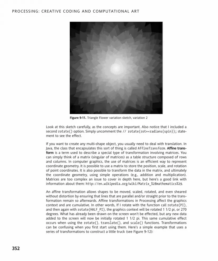
Figure 9-11. Triangle Flower variation sketch, variation 2
Look at this sketch carefully, as the concepts are important. Also notice that I included asecond rotate() option. Simply uncomment the // rotate(rot+=radians(spin)); state-ment to see the effect.
If you want to create any multi-shape object, you usually need to deal with translation. InJava, the class that encapsulates this sort of thing is called AffineTransform. Affine trans-form is a term used to describe a special type of transformation involving matrices. Youcan simply think of a matrix (singular of matrices) as a table structure composed of rowsand columns. In computer graphics, the use of matrices is an efficient way to representcoordinate geometry. It is possible to use a matrix to store the position, scale, and rotationof point coordinates. It is also possible to transform the data in the matrix, and ultimatelythe coordinate geometry, using simple operations (e.g., addition and multiplication).Matrices are too complex an issue to cover in depth here, but here’s a good link withinformation about them: http://en.wikipedia.org/wiki/Matrix_%28mathematics%29.
An affine transformation allows shapes to be moved, scaled, rotated, and even shearedwithout distortion by ensuring that lines that are parallel and/or straight prior to the trans-formation remain so afterwards. Affine transformations in Processing affect the graphicscontext and are cumulative. In other words, If I rotate with the function call rotate(PI),and then again with rotate(HALF_PI), the graphics context will be rotated 1 1/2 pi, or 270degrees. What has already been drawn on the screen won’t be effected, but any new dataadded to the screen will now be initially rotated 1 1/2 pi. This same cumulative effectoccurs when using the rotate(), translate(), and scale() functions. Transformationscan be confusing when you first start using them. Here’s a simple example that uses aseries of transformations to construct a little truck (see Figure 9-12):
PROCESSING: CREATIVE CODING AND COMPUTATIONAL ART
352
617xCH09.qxd 4/18/07 3:38 PM Page 352

//Toy Truckint truckW = 300;int truckH = 100;int truckX = -truckW/2;int truckY = -truckH/2;
void setup(){size(500, 200);background(0);smooth();
//body1translate(width-truckW/2-50, height/2);rect(truckX, truckY, truckW, truckH);
//body2translate(-width+316, 17);scale(.2, .65);rect(truckX, truckY, truckW, truckH);
//body3translate(-width+250, 20);scale(.7, .59);noStroke();rect(truckX, truckY, truckW, truckH);
//tiresstroke(255);strokeWeight(7);scale(.70, .75);translate(160, 172);ellipse(truckX, truckY, truckW, truckH);translate(1300, 0);ellipse(truckX, truckY, truckW, truckH);translate(1800, 0);ellipse(truckX, truckY, truckW, truckH);translate(400, 0);ellipse(truckX, truckY, truckW, truckH);
//window masktranslate(-3355, -284);scale(.7, .9);noStroke();fill(0);triangle(truckX, truckY + truckH, truckX+truckW, !
truckY, truckX, truckY);}
SHAPES
353
9
617xCH09.qxd 4/18/07 3:38 PM Page 353

Figure 9-12. Toy Truck sketch
When looking at the code in the last example, I hope some of you protested, exclaiming“Hey, you can’t use all those magic numbers!” It’s true, it isn’t good practice to use magicnumbers. And this really is a pretty lousy implementation of a truck (although it’s kind ofcute, don’t you think?). The problem I faced was dealing with all the accumulating matrixtransformations and having to manually plug in and try different values until I got mytruck. Because of the scaling effect, some of the translation values got pretty wacky, witha few values far exceeding the display window dimensions. Fortunately, there is a muchbetter way to handle resetting the matrix values, which I’ll discuss shortly.
The last basic shape function I’ll cover is quad(). This function works just like thetriangle() function, but uses four vertices instead of three. The function requires eightarguments, defining the x and y components of each of the four vertices. Unlike therect() function, in which each corner is 90 degrees, quad() can create a four-point poly-gon with different angles for each corner. In the following simple quad() example, I illus-trate this using the random() function for each vertex (see Figure 9-13):
// Simple Quadsize(300, 300);background(0);noStroke();smooth();// quad(p1.x, p1.y, p2.x, p2.y, p3.x, p3.y, p4.x, p4.y)quad(50+random(-25, 25), 50+random(-25, 25), !
250+random(-25, 25), 50+random(-25, 25), !250+random(-25, 25), 250+random(-25, 25), !50+random(-25, 25), 250+random(-25, 25));
PROCESSING: CREATIVE CODING AND COMPUTATIONAL ART
354
617xCH09.qxd 4/18/07 3:38 PM Page 354

Figure 9-13. Simple Quad sketch
Next is a more interesting quad() example that also includes Processing’s resetMatrix()function, used to reset the affine transformation matrix discussed earlier (see Figure 9-14):
// Disintegrating Quad Wall
float randShift = .2;int quadW = 15;int quadH = quadW;float[]q = { -quadW/2, -quadH/2, quadW, quadH };
void setup() {size(600, 600);background(255);smooth();noStroke();/* generate a table structure ofquads progressivley adding morerandomization to each quad */for (int i=0, k=1; i<height-quadH; i+=quadH, k++){/* resetting the transformation matrixkeeps the translations from continuallyaccumulating. Try commenting out theresetMatrix() call to see the effect. */resetMatrix();translate(0, quadH*k);for (int j=0; j<width-quadW; j+=quadW){translate(quadW, 0);fill(random(0, 255));// r(k) is a function callquad(q[0]+r(k), q[1]+r(k), !
SHAPES
355
9
617xCH09.qxd 4/18/07 3:38 PM Page 355

q[0]+q[2]+r(k), q[1]+r(k), !q[0]+q[2]+r(k), q[1]+q[3]+r(k), !q[0]+r(k), q[1]+q[3]+r(k));
}}
}
float r(int i){return random(-i*randShift, i*randShift);
}
Figure 9-14. Disintegrating Quad Wall sketch
PROCESSING: CREATIVE CODING AND COMPUTATIONAL ART
356
617xCH09.qxd 4/18/07 3:38 PM Page 356

This is a dense little sketch, so it may not be apparent at first glance what’s happening. Thenested for loop generates a table structure of quadrilaterals. In the outer for loop head, Iinitialized two variables (i and k) since I needed one variable to be incremented by quadH(i) and one to be incremented by 1 (k). The first line in the loop, after the comment, is thefunction call resetMatrix(). This simple step clears the transformation matrix at thebeginning of each iteration of the loop. Since the matrix was getting reset each time, Icouldn’t use it to step down the rows of the table. I solved this by multiplying the secondargument (which controls the y position) in the outer loop translate() call with k, as intranslate(0, quadH*k). However, by resetting the matrix, I was able to repeatedly calltranslate(quadW, 0) within the inner loop, which took care of stepping the quadranglesacross the display window. Finally, I set up a convenient little function, r(val), to add arandom offset to the quadrangle points. Since I used the outer loop variable k to specifythe random range, randomization increased as the loop ran. Try changing the randShiftvariable at the top of the sketch to see how it affects the output.
Before moving on to some other drawing functions, I want to provide one more examplethat will hopefully help clarify the matrix transformations. The next sketch uses a conven-ient Processing function, printMatrix(), which actually prints to the screen the currentcontents of the transformation matrix. As I mentioned earlier, transformations affect thevirtual drawing, or graphics context, so in this next example, all I include are the actualmatrix transformations—which is all I need to see how the individual transformation func-tion calls affect the overall matrix. You don’t need to spend too much time on this, but justlook at which part of the matrix is affected by each call (see Figure 9-15):
// printMatrix()//initial stateprintln(" before transformations");printMatrix();
//translatetranslate(150, 225);println(" after translate()");printMatrix();
//scalescale(.75, .95);println(" after translate() and scale()");printMatrix();
//rotaterotate(PI*.3);println(" after translate(), scale() and rotate()");printMatrix();
//resetresetMatrix();println(" after resetMatrix()");printMatrix();
SHAPES
357
9
617xCH09.qxd 4/18/07 3:38 PM Page 357

Figure 9-15. printMatrix() sketch
Plotting shapesAlthough the basic shape functions rect(), ellipse(), triangle(), and quad() offersome convenience, they are also pretty limited. Processing has a more general and versa-tile approach to shape creation that you’ve looked at before. Utilizing beginShape(),endShape(), and a series of vertex() commands, any shape can be created usingProcessing. These shapes can include combinations of both straight and curved sections.beginShape() also offers some advanced modes, allowing more complex polygonal struc-tures to be created. You’ve used these functions before, so some of this will likely bereview. I’ll begin by examining the default closed mode, which will generate a polygon (seeFigure 9-16):
//Octagonsize(400, 400);background(255);smooth();int margin = 50;fill(0);stroke(127);strokeWeight(6);beginShape();vertex(3, height/2);vertex(margin, margin);
PROCESSING: CREATIVE CODING AND COMPUTATIONAL ART
358
617xCH09.qxd 4/18/07 3:38 PM Page 358

vertex(width/2, 3);vertex(width-margin, margin);vertex(width-3, height/2);vertex(width-margin, height-margin);vertex(width/2, height-3);vertex(margin, height-margin);endShape(CLOSE);
Figure 9-16. Octagon sketch
The default beginShape() mode is a filled but open shape. By adding the CLOSE argumentto the endShape() call, the shape is closed (by connecting the last vertex to the initial ver-tex), as illustrated in the Octagon example. Plotting the octagon wasn’t too difficultbecause an 8-sided regular shape on a 4-sided window boils down to plotting vertices atthe corners and midpoints of the display window—but what about switching to a penta-gon or heptagon (7 sides), or even an enneakaidecagon (a 19-sided polygon)? Using a lit-tle trig, you can very easily create a general-purpose polygon creator. In the followingexample, I’ve parameterized lots of details to make the makePoly() function useful. I’vealso called this function a bunch of times in the sketch to showcase the range of images itcan create (see Figure 9-17).
/*Polygon CreatorIra Greenberg, December 26, 2005*/void setup(){size(600, 600);background(127);smooth();/*
SHAPES
359
9
617xCH09.qxd 4/18/07 3:38 PM Page 359

//complete parameter listmakePoly(x, y, pts, radius 1, radius 2, initial rotation, !stroke Color, stroke Weight, fill Color, endcap, stroke join)*/// makePoly function callsmakePoly(width/2, height/2, 72, 420, 270, 45, color(0, 0, 0), !
16, color(255, 255, 255));makePoly(width/2, height/2, 16, 300, 250, 45, color(200, 200, 200),!
10, color(20, 20, 20));makePoly(width/2, height/2, 60, 210, 210, 45, color(255,255,255), !
8, color(0,0,0), PROJECT, ROUND);makePoly(width/2, height/2, 60, 200, 155, 45, color(120, 120, 120),!
6, color(255, 255, 255), PROJECT, ROUND);makePoly(width/2, height/2, 50, 280, -200, 45, !
color(200, 200, 200), 6, color(50, 50, 50), PROJECT, ROUND);makePoly(width/2, height/2, 8, 139, 139, 68, color(255, 255, 255), !
5, color(0,0,0));makePoly(width/2, height/2, 24, 125, 60, 90, color(50, 50, 50), 12,!
color(200, 200, 200), ROUND, BEVEL);makePoly(width/2, height/2, 4, 60, 60, 90, color(0,0,0), 5, !
color(200,200,200), ROUND, BEVEL);makePoly(width/2, height/2, 4, 60, 60, 45, color(255, 255, 255), 5,!
color(20, 20, 20), ROUND, BEVEL);makePoly(width/2, height/2, 30, 30, 30, 90, color(75, 75, 75), 10, !
color(60,60,60), ROUND, BEVEL);makePoly(width/2, height/2, 30, 28, 28, 90, color(255, 255,255), 2,!
color(60,60,60), ROUND, BEVEL);makePoly(width/2, height/2, 24, 10, -25, 45, #000000, .75, !
color(255, 255, 255), SQUARE, MITER);}
//default - if no args passedvoid makePoly(){// call main makePoly functionmakePoly(width/2, height/2, 4, width/4, width/4, !45, #777777, 4, #AAAAAA, SQUARE, MITER);
}
// x, y, pts argsvoid makePoly(float x, float y, int pts){// call main makePoly functionmakePoly(x, y, pts, width/4, width/4, !45, #777777, 4, #AAAAAA, SQUARE, MITER);
}
PROCESSING: CREATIVE CODING AND COMPUTATIONAL ART
360
617xCH09.qxd 4/18/07 3:38 PM Page 360
// x, y, pts, rad1, rad2 argsvoid makePoly(float x, float y, int pts, float rad1, float rad2){// call main makePoly functionmakePoly(x, y, pts, rad1, rad2, 45, #777777, 4, #AAAAAA, !SQUARE, MITER);
}
// x, y, pts, rad1, rad2,, initRot, strokeCol, strokeWt, fillCol argsvoid makePoly(float x, float y, int pts, float rad1, float rad2, !float initRot, color strokeCol, float strokeWt, color fillCol){
// call main makePoly functionmakePoly(x, y, pts, rad1, rad2, initRot, strokeCol, strokeWt, !fillCol, SQUARE, MITER);
}
// main function - called by other overloaded functions/methodsvoid makePoly(float x, float y, int pts, float rad1, float rad2, !
float initRot, color strokeCol, float strokeWt, !color fillCol, int endCap, int endJoin){
float px = 0, py = 0, angle = initRot;stroke(strokeCol);strokeWeight(strokeWt);strokeCap(endCap);strokeJoin(endJoin);fill(fillCol);
beginShape();for (int i = 0; i< pts; i++){if (i%2 == 0){px = x+cos(radians(angle))*rad1;py = y+sin(radians(angle))*rad1;
}else {px = x+cos(radians(angle))*rad2;py = y+sin(radians(angle))*rad2;
}vertex(px, py);angle+=360/pts;
}endShape(CLOSE);
}
SHAPES
361
9
617xCH09.qxd 4/18/07 3:38 PM Page 361

Figure 9-17. Polygon Creator sketch
The trig functions, based on unit circle relationships, do most of the real work in thissketch. I’ve included sin() and cos() expressions in numerous examples earlier in thebook, and a general discussion about trig and the unit circle can be found in Chapter 4 andalso in Appendix B. In addition, I owe some debt to Ric Ewing, who a couple years ago pub-lished a series of wonderful drawing methods for ActionScript that have informed my ownapproach (see www.macromedia.com/devnet/flash/articles/adv_draw_methods.html).
I nested the trig functions in a conditional if...else structure as a simple way to gener-ate two radii. I’ve used this technique in other places in the book as well. The modulusoperator, %, returns the remainder of the division between the two operands (e.g., 9 % 5 =4, as 5 goes into 9 once, leaving a remainder of 4). I used (i%2 == 0) in the head of theconditional so that points would alternate between radius 1 and radius 2. If you don’t seeit yet, this works because only even numbers will return 0, but odds won’t.
The other possibly surprising aspect of this sketch is the use of five makePoly() functiondefinitions, in which—in all but one of them—another makePoly() function is called. Thisapproach of creating multiple functions (or methods) with the same name is a commontechnique in OOP, and is referred to as method overloading. As long as the method signa-tures are different, the compiler sees them as unique structures. The signature, in Java andProcessing, is a combination of the method name and parameter list (including the num-ber and type of parameters). If the number and/or type of parameters is different inthe signatures, then the compiler sees the methods as unique, regardless of whether themethods share the same name. This is a convenient implementation, as it gives users achoice of how to call/use the method.
PROCESSING: CREATIVE CODING AND COMPUTATIONAL ART
362
617xCH09.qxd 4/18/07 3:38 PM Page 362

I created five versions of the makePoly() function. It is possible to create a lot more,although it’s probably not necessary. Only one of the makePoly() functions includes thefull parameter list; the others use a partial list, and one of them includes no parameter.Each of the four makePoly() functions (without the full parameter list) internally calls themakePoly() function with the full list. I did this so that the actual plotting algorithm couldbe put in one place—inside the makePoly() function with the full parameter list.
When one of the functions without the full parameter list is called, it internally passes thearguments it received—adding default values for the remaining ones—to the makePoly()function with the full parameter list and plotting implementation. I recommend trying toadd your own version of a makePoly() function to the sketch to get a better sense of howthis all works.
Regular and star polygons are fine, but there are some other useful shapes that you canbuild by modifying the last algorithm a bit. Here’s a sprocket creator sketch, in which I callthe makeSprocket()function a bunch of times to demonstrate the range of shapes thefunction is capable of generating (see Figure 9-18).
/*Sprocket CreatorIra Greenberg, December 27, 2005*/
void setup(){size(600, 600);background(65);smooth();
makeSprocket(width/2, height/2, 20, 280, 440, 45, color(0, 0, 0), !20, color(255, 255, 255), SQUARE, MITER);
makeSprocket(width/2, height/2, 120.0, 275, -230, 45, !color(200, 200, 200), 2, color(20, 20, 20), SQUARE, ROUND);
makeSprocket(width/2, height/2, 20.0, 250, 120, 45, color(0, 0, 0),!12, color(255, 255, 255), PROJECT, MITER);
makeSprocket(width/2, height/2, 8.0, 120, 190, 45, !color(20, 20, 20), 14, color(200, 200, 200), PROJECT, MITER);
makeSprocket(width/2, height/2, 8.0, 120, 170, 22.5, !color(245, 245, 245), 20, color(10, 10, 10), PROJECT, MITER);
makeSprocket(width/2, height/2, 25.0, 90, 35, 45, !color(255, 255, 255), 2, color(0, 0, 0), PROJECT, MITER);
makeSprocket(width/2, height/2, 8.0, 25, 10, 45, !color(127, 127, 127), 4, color(255, 255, 255), PROJECT, MITER);
}
void makeSprocket(float x, float y, float spokes, float rad1, !float rad2, float initRot, color strokeCol, float strokeWt, !color fillCol, int endCap, int endJoin){
SHAPES
363
9
617xCH09.qxd 4/18/07 3:38 PM Page 363

float px = 0, py = 0, angle = initRot;float ang = (360.0/spokes)/2.0;float ang2 = (360.0/spokes)/4.0;stroke(strokeCol);strokeWeight(strokeWt);strokeCap(endCap);strokeJoin(endJoin);fill(fillCol);
beginShape();for (int i = 0; i<spokes; i++){px = x+cos(radians(angle))*rad1;py = y+sin(radians(angle))*rad1;vertex(px, py);angle+=ang;px = x+cos(radians(angle))*rad1;py = y+sin(radians(angle))*rad1;vertex(px, py);angle+=ang2;px = x+cos(radians(angle))*rad2;py = y+sin(radians(angle))*rad2;vertex(px, py);angle+=ang2;
}endShape(CLOSE);
}
Figure 9-18. Sprocket Creator sketch
PROCESSING: CREATIVE CODING AND COMPUTATIONAL ART
364
617xCH09.qxd 4/18/07 3:38 PM Page 364

The Sprocket Creator sketch is similar to the Polygon Creator sketch. The main differenceis the few extra trig expressions in the makeSprocket() function. Instead of plotting ver-tices at equal angle rotations, each spoke of the sprocket is composed of three vertices.The first and second share the same radius and are the outer edge of the spoke. The thirdvertex is an inner radius, and is at the base between each spoke. Notice also that I usedtwo different angle values. I somewhat arbitrarily defined the angle between the twospoke vertices (within the spoke) as twice as large as the angle between the spokes. Thefinal angle incrementation (angle+=ang2) ensures that there is symmetry between eachspoke.
As reading descriptions like this can be confusing, I suggest playing with the sketch andcreating some of your own sprockets. You might also want to try to spin your own shapeby modifying the existing drawSprocket() method.
Creating hybrid shapesThe beginShape() and endShape() functions allow you to combine straight and curvedlines to form hybrid shapes. Once you introduce curves into to your shapes, calculatingcoordinates can get a little tricky. It often helps to break the problem down into moremanageable sections—in the next two example sketches, I do just that. In the first sketch,I hack out a list of coordinates (using magic numbers) and individual drawing function callsthat create a hybrid shape. In the second sketch, I develop a more general plotting algo-rithm, removing all the magic numbers. Here’s the initial code in all its magic number glory(see Figure 9-19):
// Hybrid Shapesize(600, 600);curveTightness(-.4);smooth();
beginShape();curveVertex(200, -300);curveVertex(200, 100);curveVertex(400, 100);curveVertex(400, -300);
vertex(500, 100);vertex(500, 200);
curveVertex(800, 200);curveVertex(500, 200);curveVertex(500, 400);curveVertex(800, 400);
vertex(500, 500);vertex(400, 500);
SHAPES
365
9
617xCH09.qxd 4/18/07 3:38 PM Page 365

curveVertex(400, 800);curveVertex(400, 500);curveVertex(200, 500);curveVertex(200, 800);
vertex(100, 500);vertex(100, 400);
curveVertex(-200, 400);curveVertex(100, 400);curveVertex(100, 200);curveVertex(-200, 200);
vertex(100, 100);endShape(CLOSE);
Figure 9-19. Hybrid Shape sketch
The next step was looking at the ugly code I had written and seeing if I could figure out analgorithm to generalize the form. This backward approach—making before thinking—seems to be a general pattern I use when I get stuck. I guess if you’re better at math thanme, you might be able to lay down clean algorithms by just thinking about problems, butI usually have to get my hands dirty first. Because the shape created in the sketch is sym-metrical, and there is a recurring pattern of function calls in the code, I knew it would bepossible, without too much hair pulling, to figure out the algorithm. I also knew, becauseof the radial symmetry, that using trig functions would somehow be the easiest solution.Here’s what I got (see Figure 9-20):
PROCESSING: CREATIVE CODING AND COMPUTATIONAL ART
366
617xCH09.qxd 4/18/07 3:38 PM Page 366

// Hybrid Shape 2size(600, 600);curveTightness(-.4);smooth();strokeWeight(10);float sides = 8;float angle = 360.0/sides/2;float px = 0, py = 0;float cx = 0, cy = 0;float ang = 360.0/(sides+sides/2.0);float ang2 = ang/2.0;float rad1 = 250.0;float rad2 = rad1*2.0;int x = width/2;int y = height/2;
beginShape();for (int i=0; i<sides; i++){cx = x+cos(radians(angle))*rad2;cy = y+sin(radians(angle))*rad2;curveVertex(cx, cy);px = x+cos(radians(angle))*rad1;py = y+sin(radians(angle))*rad1;curveVertex(px, py);angle+=ang;px = x+cos(radians(angle))*rad1;py = y+sin(radians(angle))*rad1;curveVertex(px, py);cx = x+cos(radians(angle))*rad2;cy = y+sin(radians(angle))*rad2;curveVertex(cx, cy);px = x+cos(radians(angle))*rad1;py = y+sin(radians(angle))*rad1;vertex(px, py);angle+=ang2;px = x+cos(radians(angle))*rad1;py = y+sin(radians(angle))*rad1;vertex(px, py);
}endShape(CLOSE);
SHAPES
367
9
617xCH09.qxd 4/18/07 3:38 PM Page 367

Figure 9-20. Hybrid Shape 2 sketch
This sketch makes a good gear shape. If you change the value of the sides variable in theexample, the shape scales nicely. I think it would be a good exercise to try to “functional-ize” this last example. In other words, try sticking the main drawing routine in a functionwith a bunch of parameters, as I did with the polygon and sprocket examples. BesidescurveVertex(), you can also use bezierVertex() in conjunction with regular vertex()calls, but I’ll also leave that for you to try on your own.
The other shape modesThere are a number of additional shape modes. Many of these are more applicable to 3Dthan 2D, for creating a skin or polygonal mesh around a 3D form. In the 3D chapters, you’lllearn how to plot some 3D forms. For now, I’m just going to give a brief overview of whatthe other modes do. The first two you’ll look at, TRIANGLES and QUADS, don’t form a con-tiguous mesh, but rather simply create individual triangles and quadrangles from lists ofcoordinates. In the next example, I’ll generate 90 triangles using a for loop and theTRIANGLES mode (see Figure 9-21):
//Random Trianglessize (500, 500);background(255);smooth();beginShape(TRIANGLES);for (int i=0; i<90; i++){stroke(random(0, 200));fill(random(225, 255), 150);strokeWeight(random(.5, 5));vertex(random(width), random(height));
}endShape();
PROCESSING: CREATIVE CODING AND COMPUTATIONAL ART
368
617xCH09.qxd 4/18/07 3:38 PM Page 368

Figure 9-21. Random Triangles sketch (TRIANGLES mode)
Although you could relatively easily write your own function to pull this sort of thing off,it is still convenient having this option. It would be a good exercise to try to re-create thefunctionality of the beginShape(TRIANGLES) mode using the triangle() function orthe no-argument version of beginShape().
Notice the extra argument in the command fill(random(225, 255), 150);, after theclosed parentheses of the random call. This optional second argument allows you to con-trol the alpha, or transparency, of the grayscale fill. The value range is from 0 to 255(0 being transparent and 255 being completely opaque). If you don’t specify an argument,the default value is 255. The stroke() and fill() commands each allow you to specifyone, two, three, or four arguments. In the next chapter, I’ll discuss color and imaging, andconcepts like alpha in greater detail.
beginShape(QUADS) mode works similarly to TRIANGLE mode, except that shapes areclosed in groups of four vertex() calls instead of three. In this next example, I generaterandom quads, bounded within a rectangular region, forming a sort of shape texture (seeFigure 9-22).
//Random Bounded Quadssize (250, 250);background(255);smooth();int[]boundinBox = {50, 50, 150, 150};fill(0);
SHAPES
369
9
617xCH09.qxd 4/18/07 3:38 PM Page 369

rect(boundinBox[0], boundinBox[1], boundinBox[2], boundinBox[3]);strokeJoin(BEVEL);beginShape(QUADS);for (int i=0; i<1000; i++){stroke(random(50, 255));fill(0, 0);strokeWeight(random(.5, 2));vertex(random(boundinBox[0], boundinBox[0]+boundinBox[2]), !
random(boundinBox[1], boundinBox[1]+boundinBox[3]));}endShape();
Figure 9-22. Random Bounded Quads sketch (QUADS mode)
You’ll notice in the output that the shapes don’t form a pattern of little rectangles, eventhough they were generated by using QUADS mode. This is because a quadrilateral is notnecessarily a rectangular structure. It is possible to create a quadrilateral in which notwo sides are parallel; this shape is sometimes referred to as a trapezium. If any two of thesides are parallel, it’s usually called a trapezoid, which I assume you remember from somemath class. There is a simple and complex classification for polygons, which affects quadri-laterals as well. Simple polygons don’t intersect with themselves, while complex ones do.Here’s an example of each, using QUADS mode (see Figure 9-23):
//Simple/Complex Quadssize (300, 150);smooth();beginShape(QUADS);//simple quadvertex(25, 40);vertex(125, 30);
PROCESSING: CREATIVE CODING AND COMPUTATIONAL ART
370
617xCH09.qxd 4/18/07 3:38 PM Page 370

vertex(120, 120);vertex(20, 118);//complex quadvertex(175, 40);vertex(275, 30);vertex(170, 118);vertex(270, 120);endShape();
Figure 9-23. Simple/Complex Quads sketch
Simple vs. complex polygons is a big issue in 3D, where quadrilateral surfaces can becomenon-planar and cause anomalies when rendering. Triangles, on the other hand, are alwaysplanar. For our current purposes, in 2D, complex quads just form an interesting pattern. Ifyou want to learn more about quads in general, check out http://en.wikipedia.org/wiki/Quadrilateral (I especially like the taxonomic classification chart). One other minorbut significant point about using either TRIANGLE or QUADS mode is that you’ll want tomake sure that you use the right number of vertex() commands. The number of com-mands should be divisible by 3 for TRIANGLES and 4 for QUADS. Additional vertex() linesthat aren’t grouped in three or four lines, respectively, will be disregarded. For example,as shown in Figure 9-24, the fourth and fifth lines in the following sequence will bedisregarded:
size (120, 120);beginShape(TRIANGLES);vertex(20, 20);vertex(100, 100);vertex(40, 100);vertex(30, 60);vertex(20, 50);endShape();
SHAPES
371
9
617xCH09.qxd 4/18/07 3:38 PM Page 371

Figure 9-24. Disregarded extra vertex() calls
The last three modes I’ll discuss briefly are TRIANGLE_STRIP, TRIANGLE_FAN, andQUAD_STRIP. These modes build contiguous meshes of polygons, which is very useful in 3D.They work sort of similarly to the last two modes discussed, except that the multiple formscreated are attached. Also, extra vertex() lines are not disregarded. However, a minimumnumber of vertex() commands need to be issued—three for TRIANGLE_STRIP andTRIANGLE_FAN, and four for QUAD_STRIP—before any shapes are rendered. Here’s anexample using TRIANGLE_STRIP mode (see Figure 9-25):
// TRIANGLE_STRIP Modesize(400, 400);smooth();int x = width/2;int y = height/2;int outerRad = 150;int innerRad = 200;float px = 0, py = 0, angle = 0;float pts = 36;float rot = 360.0/pts;
beginShape(TRIANGLE_STRIP);for (int i=0; i<pts; i++) {px = x+cos(radians(angle))*outerRad;py = y+sin(radians(angle))*outerRad;angle+=rot;vertex(px, py);px = x+cos(radians(angle))*innerRad;py = y+sin(radians(angle))*innerRad;vertex(px, py);angle+=rot;
}endShape();
PROCESSING: CREATIVE CODING AND COMPUTATIONAL ART
372
617xCH09.qxd 4/18/07 3:38 PM Page 372

Figure 9-25. TRIANGLE_STRIP Mode sketch
I reused the basic trig functions I’ve been using throughout the book for generating anellipse. By setting an outer and inner radius, this shape could be useful as an end cap for ahollow 3D cylinder. Next, I simply decreased the radii and fill color value (from white toblack) each loop iteration, creating a spiral (see Figure 9-26):
// TRIANGLE_STRIP Spiralsize(400, 400);background(0);smooth();int x = width/2;int y = height/2;int outerRad = 160;int innerRad = 200;float px = 0, py = 0, angle = 0;int pts = 36;float rot = 360.0/pts;int fillCol = 255;int fillfade = fillCol/pts;
beginShape(TRIANGLE_STRIP);for (int i=0; i<pts; i++) {px = x+cos(radians(angle))*outerRad;py = y+sin(radians(angle))*outerRad;angle+=rot;vertex(px, py);px = x+cos(radians(angle))*innerRad;py = y+sin(radians(angle))*innerRad;vertex(px, py);outerRad-=4;
SHAPES
373
9
617xCH09.qxd 4/18/07 3:38 PM Page 373

innerRad-=4.25;fill(fillCol);fillCol-=fillfade;angle+=rot;
}endShape();
Figure 9-26. TRIANGLE_STRIP Spiral sketch
TessellationAnother interesting thing you can do with these functions is create a tessellation. Atessellation is a pattern of shapes that fit together, without any gaps, covering a surface.For more of a definition, have a look at what Wikipedia has to say about tessellations, athttp://en.wikipedia.org/wiki/Tessellation. TRIANGLE_FAN mode is a little tricky, as itneeds to rotate clockwise, and the initial point should define the center part of the fan. In3D, forms are commonly converted to and/or rendered as triangle meshes. TRIANGLE_FANmode is a somewhat convenient function for triangulating planar geometry. Triangulatingmeans converting a larger polygon into triangles, which is a form of tessellation. Since tri-angles are always planar and simple (with regard to polygons—not a commentary on theirintelligence), they are easier for the computer to render than quadrilaterals. This mode
PROCESSING: CREATIVE CODING AND COMPUTATIONAL ART
374
617xCH09.qxd 4/18/07 3:38 PM Page 374

works by defining the center point of the fan and then selecting the vertices in a clockwisefashion along the perimeter of the shape you want to triangulate. Once again, the trigfunctions come in handy. Here’s an example sketch that triangulates any regular polygon,using TRIANGLE_FAN mode (see Figure 9-27):
//TRIANGLE_FANsize(400, 400);smooth();strokeWeight(1.5);float px = 0, py = 0;float angle = 0;float radius = 150;int pts = 8;int x = width/2;int y = height/2;
// needs to rotate clockwisebeginShape(TRIANGLE_FAN);vertex(x, y);for (int i=0; i<=pts; i++){px = x+cos(radians(angle))*radius;py = y+sin(radians(angle))*radius;vertex(px, py);angle+=360/pts;
}
Figure 9-27. TRIANGLE_FAN sketch
SHAPES
375
9
617xCH09.qxd 4/18/07 3:38 PM Page 375

Next, I’ll use the last solution as part of a sketch for a tessellated plane (see Figure 9-28):
/*Tessellated PlaneIra Greenberg, December 30, 2005*/void setup(){size(400, 400);smooth();tesselate(6, 20);
}
void tesselate(int points, int radius){/* catch and handle out ofrange point count */if (points<=5){points = 4;
}else {points = 6;
}
// eventually add some more patternsswitch(points){case 4:for (int i = 0, k = 0; i<=width+radius; i+=radius*2, k++){for (int j = 0; j<=height+radius; j+=radius*2){drawPoly(i-radius, j-radius, points, 0, radius);drawPoly(i, j, points, 0, radius);
}}break;
case 6:for (float i = 0, k = 0; i<=width+radius; i+=radius*1.5, k++){for (float j = 0; j<=height+radius*2; j+=(cos(radians(30))* !
radius)*2){if (k%2==0){drawPoly(i, j-cos(radians(30))*radius, points, 0, radius);
}else{drawPoly(i, j, points, 0, radius);
}}
}break;
}}
PROCESSING: CREATIVE CODING AND COMPUTATIONAL ART
376
617xCH09.qxd 4/18/07 3:38 PM Page 376

// draw triangle fanvoid drawPoly(float x, float y, int pts, float initAngle, float rad){strokeWeight(1.5);float px = 0, py = 0;float angle = initAngle;// needs to rotate clockwisebeginShape(TRIANGLE_FAN);vertex(x, y);for (int i=0; i<=pts; i++){fill(255/pts*i);px = x+cos(radians(angle))*rad;py = y+sin(radians(angle))*rad;vertex(px, py);angle+= 360/pts;
}}
Figure 9-28. Tesselated Plane sketch
This last example is fairly complex; though not much is new. It took some finessing to getthe geometry to tile properly and a bit of trig for the hexagon tiling. There are two thingsthat I think are significant about this sketch. The first involves encapsulation and the latterinvolves exception handling. Both custom functions tessellate() and drawPoly() involve
SHAPES
377
9
617xCH09.qxd 4/18/07 3:38 PM Page 377

somewhat complicated implementations. However, to use both functions in the last exam-ple, all that needed to be called was tessellate(6, 20);. When you encapsulate proce-dural complexity into self-contained modular units such as functions, it becomes relativelysimple to use even the most complexly implemented procedures. This illustrates a generalnotion of the concept of encapsulation. There is also the more specific but related defini-tion of encapsulation (discussed in Chapter 8) that applies specifically to OOP.
The second point, exception handling, is illustrated by the conditional statement at the topof the tessellate() function. The conditional syntax you’ve seen before, but the conceptis new. I only wrote tessellation routines for four- and six-sided polygons. However, some-one could conceivably use the function at some point and put in a value other than 4 or 6.Rather than generate an unexpected error, I wrote code to catch the out-of-range valueand correct it. Eventually, additional tessellation routines could be added to the program,at which time you would simply update the conditional. The concept of building in codestructures to catch and deal with input errors is generally referred to as exceptionhandling. In a language like Java, exception handling is formalized, with numerous classstructures. Processing doesn’t have its own native exception handling structures (butyou’re free to use Java’s structures). Generally speaking, though, a formalized exceptionhandling process is beyond what most people will want to do with Processing. In addition,the places where exception handling is required in Processing (e.g., input/output) arealready encapsulated and invisible to the user. Remember that this is kind of the wholepoint of Processing—to minimize the annoying lower-level stuff, allowing people to morefreely express themselves. So there may be times, as in my last example, that you mightwant to build in some simple safety checks. If, however, you do end up building somethingthat you feel requires a more elaborate and formal error-checking system, you’ll want tolook into Java’s exception handling capabilities. Here’s some info from Sun: http://java.sun.com/docs/books/tutorial/essential/exceptions/.
Applying OOP to shape creationThe last section of this chapter utilizes an OOP approach. Chapter 8 dealt exclusively withOOP, but I’ll review some of the fundamental concepts here as well. OOP is not easy fornew coders to get their heads around, so try not to be too hard on yourself if you findsome of the material difficult—it really is.
The “object-oriented” part of OOP is an approach to programming that treats concepts(both things and processes) as self-contained modular units. These units, called classes, arelike blueprints describing a concept, which includes attributes (properties) and functions(methods) contained within the class definition. For example, if you create a class calledRectangle, the properties of this class might include its x and y position, its width andheight, its stroke and fill color, and so on. Its methods might include getting and setting itswidth or height, and drawing itself. To use the Rectangle class, you create (instantiate)objects from it. Since the class is like a blueprint, when you make an object, you get a copyof all the properties and methods defined in the class; and each object remains independ-ent from all the other objects made from the same class. This allows you to have ten rec-tangle objects, each with different postion, size, color, and so on. Since I’ve gone this farwith the rectangle metaphor, let’s actually constuct a simple rectangle class and imple-ment it in Processing.
PROCESSING: CREATIVE CODING AND COMPUTATIONAL ART
378
617xCH09.qxd 4/18/07 3:38 PM Page 378

void setup(){// create new rectangle objectnew Rectangle();
}
// class descriptionclass Rectangle {}
This is all it takes to create a class in Processing. Of course, this class won’t do anything, butit’s a start. To create a class, you use the class keyword followed by the name of the class.You capitalize the name of your classes. To create an object from the Rectangle class, youuse the new keyword. Typically, you also assign the new object to a variable so that you canrefer to it later in your program. In the last example, even though I created a Rectangleobject, I can’t communincate with it, as there is no variable assigned a reference to theobject. Figure 9-29 shows an improved (and more useful) version of the last sketch:
// object (reference) variableRectangle r1;
void setup(){// create new rectangle objectr1 = new Rectangle(100, 200, 150, 150);
}
// class descriptionclass Rectangle {
//class constructorRectangle(int x, int y, int w, int h) {println("x pos = "+ x+"\ny pos = " + y);println("width = "+ w+"\nheight = " + h);
}}
Figure 9-29. OOP println() output example
SHAPES
379
9
617xCH09.qxd 4/18/07 3:38 PM Page 379

This wasn’t much of an improvement, but I got some output at least. However, there are abunch of new concepts to discuss in this sketch. At the top of the program, I declared avariable of type Rectangle. Remember that variables in Processing and Java need to bedeclared of a data type. The data type controls things like how much memory is allocatedto the variable and what type of data the variable can be assigned. As I discussed earlier inthe book, there are two types of variables in Processing: primitive and reference.
Primitive variables, which were discussed extensively in Chapter 3, are assigned actualvalues. int, float, and char are examples of primitive variable types. Primitive variablesare relativley simple for the computer to handle, as each evaluates to a single value.
Reference variables are more complex, as they each often need to refer to multiple values.To solve this problem, reference variables, rather than directly being assigned a value, holda reference or link to the data in memory. Thus, the Rectangle r1 variable will ultimatelyhold a reference to the Rectangle object data, not the data directly. There are someimportant issues due to this arrangement, but nothing you need to worry about right now.The important point to remember is that the data type of the variable dictates what typeof data can be assigned to it; and each class you create is a unique data type. Rectangler1 can be assigned object references of the Rectangle type (or a subclass of the Rectangletype), but it can’t be assigned an int or a String value or reference of another data type.
Looking at the class definition, you’ll notice that I added a constructor. Remember that theconstructor begins with the same name as the class and also utilizes parentheses for aparameter list. When an object is created from a class, a constructor inside the class isalways run. You can think of a constructor as an object initializer function. If you don’texplicitly include a constructor, a default (internal) class constructor is called that has noparameters. By creating my own constructor, new Rectangle objects will now use my con-structor, instead of the default one. Therefore, if a Rectangle object is now created with-out four int arguments, an errror will occur. Try replacing r1 = new Rectangle(100, 200,150, 150); with r1 = new Rectangle(); to see what happens. When the constructor iscalled successfully, the code within its block (between the curly braces) is executed.
In this revised version of the sketch, the constructor outputs some sensational informationabout the Rectangle object’s properties. (Don’t worry, you’ll make some images eventu-ally.) Also notice the syntax I used in the println() commands. I generated four lines ofoutput with just two println() calls by using the newline escape sequence, \n. Escapesequences are little character shortcuts you can include in strings to do things like add anew line or include special characters. For example, if you need to include a quote char-acter in output, you’d do it like this: println("\"Help! I'm surrounded by quotes\"");.For a list of escape character sequences, check out http://java.sun.com/docs/books/jls/second_edition/html/lexical.doc.html. Finally, the following code gets theRectangle class to actually draw something (see Figure 9-30):
// Drawing with OOP// object (reference) variableRectangle r1;
void setup(){size(400, 400);background(255);
PROCESSING: CREATIVE CODING AND COMPUTATIONAL ART
380
617xCH09.qxd 4/18/07 3:38 PM Page 380

// create new rectangle objectr1 = new Rectangle(100, 200, 150, 150);
}
// class descriptionclass Rectangle {
//class constructorRectangle(int x, int y, int w, int h) {rect(x, y, w, h);}
}
Figure 9-30. Drawing with OOP sketch
Creating a neighborhoodHopefully, this last sketch makes some sense. Don’t worry if it doesn’t yet. Also, you’d becorrect in thinking that it doesn’t really make much sense to go through the bother ofcreating a class just to call rect(), which you could call from within setup(). This is cer-tainly true. So let’s add some stuff to make all this class business worth it. Let’s build asimple house, with a door, some windows, and a roof, and then let’s put a couple housestogether to form a little neighborhood. I’m going to make a class for each of the followingelements: door, window, roof, and house. In this example, I’ll keep things simple by notadding decorative features like paint, shingles, cornices, and so on. And I’ll keep all theclasses within the same PDE file (which isn’t really necessary). Later in the book, I’ll showyou how to begin working with multiple files in separate Processing tabs.
SHAPES
381
9
617xCH09.qxd 4/18/07 3:38 PM Page 381

Door classIn designing these really simple classes, it helps to think a little bit about how the housewill fit together. I’ll begin with the door—what properties will the door have? I want tokeep everything really simple for now. The door will have an x position, a y position, widthand height, and a doorknob. What methods will the door have? Working in pure Java, Iwould set up a set and get method for each of the properties. For example, for the x prop-erty, I’d have a setX() and a getX() method. In addition, in pure Java, I’d make theproperties private, meaning that users couldn’t call the properties directly (e.g., d1.x), butwould be forced to use the respective set and get methods for each property (e.g.,d1.getX()). Although this is the classic OOP approach, it is not really the Processingapproach. So I won’t make the properties private, nor will I create set and get methods forall the properties, which will actually save me a ton of work. The only methods I will addto the Door class are setknob() and drawDoor(). The setknob() method will control theside of the door on which the doorknob is drawn, and the drawDoor() method will drawthe door. Here’s the Door class:
class Door{// instance propertiesint x;int y;int w;int h;
// for knobint knobLoc = 1;
// constants - class propertiesfinal static int RT = 0;final static int LFT = 1;
// constructorDoor(int w, int h){this.w = w;this.h = h;
}
// draw the doorvoid drawDoor(int x, int y) {rect(x, y, w, h);int knobsize = w/10;if (knobLoc == 0){//right sideellipse(x+w-knobsize, y+h/2, knobsize, knobsize);
}else {//left sideellipse(x+knobsize, y+h/2, knobsize, knobsize);
}}
PROCESSING: CREATIVE CODING AND COMPUTATIONAL ART
382
617xCH09.qxd 4/18/07 3:38 PM Page 382

// set knob positionvoid setKnob(int knobLoc){this. knobLoc = knobLoc;
}}
At the top of the class, I declared some variables. The first five variables are properties thateach Door object will have access to; these are called, in OOP terminology, instance vari-ables or object properties. Each Door object will have its own unique set of these variables,so an object can assign its own values to the variables without affecting any other Doorobjects. For the doorknob, I needed some variables to specify which side of the door theknob should be on. I created two variables, LFT and RT, which I declared as constants. Iused the Java keyword final to specify that the value of the two constants can’t bechanged—which is precisely what a constant is. Secondly, I used the Java keyword staticto specify that these constants are static variables, also sometimes referred to as classvariables.
Static variables, unlike instance variables, are not unique to each object created from theclass. Instead they each hold a single value, accessible from any class, using the syntaxclass name.property. For example, if I wanted to use the Door class’s LFT property, Iwould simply write Door.LFT. I don’t need to create an object to do this, and I can do itfrom any class. So theoretically, if you ever needed the value 1, you could use Door.LFT.However, I don’t recommend doing that unless using the constant name makes sense inthe context of the program, as in setKnob(Door.LFT);. You’ll see more how these con-stants are used shortly, when an actual door is created.
The next code block is the constructor, in which I included two parameters for the door’swidth and height (which is perhaps the measurements you’d think about if you were toactually purchase a door). OOP is modeled after the physical world, so it’s not a bad ideawhen designing classes to think about how you would accomplish the same task in the realworld. Within the constructor block are two possibly odd looking assignments (althoughthey’re discussed in Chapter 8):
this.w = w;this.h = h;
Since the instance variables declared at the top of the class and the parameters specifiedbetween the parentheses of the constructor have the same identifiers (names), I need away to identify which is which. I could have simply given the parameters different namesfrom the instance variables. However, it is pretty common practice to use the samenames for instance variables and parameters in the constructor, and I tend to like doing it.
The parameters represent the values that will be passed into the constructor when anobject is created. These values will need to be seen throughout the class. However, param-eters only have local scope (meaning they can only be “seen” within the method or func-tion they’re declared in). This is a problem if another method in the class wants to be ableto access these values. By assigning the value of the parameters to the instance variablesdeclared at the top of the class—giving them global scope—the values can now be seenthroughout the class. Since the parameters have this special relationship to their partnerinstance variables, I find it convenient to give them the same name.
SHAPES
383
9
617xCH09.qxd 4/18/07 3:38 PM Page 383

Outside of the constructor, w and h always refer to the values of the instance variables bythose names. But in the constructor, w and h refer to the values of the parameters. That’sbecause local scope takes precedence over global scope. By using the special keywordthis preceding the instance variable names (connected with a dot), this.w and this.hare now seen as the instance variables, not the parameters. The w and the h, when not pre-ceded with this, are still the parameters.
Let’s skip the drawDoor() method for a moment and look at the setKnob() method. Thismethod contains another assignment, similar to the ones in the constructor. In thedrawDoor() method, which I’ll discuss next, you’ll need to know which side to drawthe doorknob on. By assigning a value to the knobLoc instance variable in the setKnob()method, the drawDoor() method will now be able to assess the side on which to attach theknob. Notice also that at the top of the class I gave the knobLoc variable an initial valuewhen I declared it. I did this just in case a position wasn’t eventually specified using thesetKnob() method.
Finally, in the drawDoor() method, I simply draw the door, using Processing’s rect() func-tion. Using a conditional statement and the knobLoc property, the method also figures outwhich side to draw the knob on, which it then does using Processing’s ellipse() function.The next sketch uses the Door class to actually draw a door (see Figure 9-31):
// Drawing a Door// object (reference) variableDoor door1;
void setup(){size(200, 350);background(200);smooth();
// create new Door objectdoor1 = new Door(100, 250);door1.setKnob(Door.LFT);door1.drawDoor(50, 50);
}
class Door{//door propertiesint x;int y;int w;int h;
// for knobint knobLoc = 1;//constantsfinal static int RT = 0;final static int LFT = 1;
PROCESSING: CREATIVE CODING AND COMPUTATIONAL ART
384
617xCH09.qxd 4/18/07 3:38 PM Page 384

// constructorDoor(int w, int h){this.w = w;this.h = h;
}
// draw the doorvoid drawDoor(int x, int y) {rect(x, y, w, h);int knobsize = w/10;if (knobLoc == 0){//right sideellipse(x+w-knobsize, y+h/2, knobsize, knobsize);
}else {//left sideellipse(x+knobsize, y+h/2, knobsize, knobsize);
}}
// set knob positionvoid setKnob(int knobLoc){this. knobLoc = knobLoc;
}}
The three lines at the top of the sketch create the door.
door1 = new Door(100, 250);door1.setKnob(Door.LFT);door1.drawDoor(50, 50);
Figure 9-31. Drawing a Door sketch
SHAPES
385
9
617xCH09.qxd 4/18/07 3:38 PM Page 385

First, I need to create the Door object; in OOP this is called instantiation. Then I optionallyset its knob position. Notice how I used the static variable LFT, preceded by the class nameand a dot. Finally, the door is drawn. Look carefully at the syntax—the door object door1is attached directly to its method with a dot. If you eventually wanted to change the valueof one of the properties, you’d target it the same way. For example, to change the x prop-erty to 194, you’d write: door1.x = 194. Of course, this command would have to comeafter the Door object has been instantiated: door1 = new Door(100, 250);. Before youmove on to the Window class, I strongly recommend you review the Door class a few times,as well as my description. I also suggest trying to make some more doors on your own. Thislittle sketch covers a lot of important issues that will be built upon.
Window classA window shares certain characteristics with a door. Both have an x and y position, as wellas width and height. If this example were more detailed, both objects might also havecolor, material, price, and inventory number characteristics. There is a way of minimizingthis redundancy between classes in OOP, called inheritance (covered extensively inChapter 8), in which classes can inherit properties and methods from other classes.However, inheritance adds another level of abstraction and complexity, so for this exampleI’ll redundantly create the same properties in the different classes. Later on in the book,when you’re an advanced object-oriented programmer, you’ll apply inheritance. Here’s asketch that draws three windows using the new Window class (see Figure 9-32):
// Drawing Some Windowsvoid setup(){size(450, 250);background(200);smooth();
Window window1 = new Window(100, 150);window1.drawWindow(50, 50);Window window2 = new Window(100, 150, true, Window.DOUBLE);window2.drawWindow(175, 50);Window window3 = new Window(100, 150, true, Window.QUAD);window3.drawWindow(300, 50);
}
class Window{//window propertiesint x;int y;int w;int h;
// customized featuresboolean hasSash = false;
PROCESSING: CREATIVE CODING AND COMPUTATIONAL ART
386
617xCH09.qxd 4/18/07 3:38 PM Page 386
// single, double, quad paneint style = 0;//constantsfinal static int SINGLE = 0;final static int DOUBLE = 1;final static int QUAD = 2;
// constructor 1Window(int w, int h){this.w = w;this.h = h;
}// constructor 2Window(int w, int h, int style){this.w = w;this.h = h;this.style = style;
}// constructor 3Window(int w, int h, boolean hasSash, int style){this.w = w;this.h = h;this.hasSash = hasSash;this.style = style;
}
// draw the windowvoid drawWindow(int x, int y) {//local variablesint margin = 0;int winHt = 0;int winWdth = 0;
if (hasSash){margin = w/15;
}
switch(style){case 0://outer window (sash)rect(x, y, w, h);//inner windowrect(x+margin, y+margin, w-margin*2, h-margin*2);break;
case 1:winHt = (h-margin*3)/2;//outer window (sash)rect(x, y, w, h);
SHAPES
387
9
617xCH09.qxd 4/18/07 3:38 PM Page 387

//inner window (top)rect(x+margin, y+margin, w-margin*2, winHt);//inner windows (bottom)rect(x+margin, y+winHt+margin*2, w-margin*2, winHt);break;
case 2:winWdth = (w-margin*3)/2;winHt = (h-margin*3)/2;//outer window (sash)rect(x, y, w, h);//inner window (top-left)rect(x+margin, y+margin, winWdth, winHt);//inner window (top-right)rect(x+winWdth+margin*2, y+margin, winWdth, winHt);//inner windows (bottom-left)rect(x+margin, y+winHt+margin*2, winWdth, winHt);//inner windows (bottom-right)rect(x+winWdth+margin*2, y+winHt+margin*2, winWdth, winHt);break;
}}
// set window style (number of panes)void setStyle(int style){this.style = style;
}}
Figure 9-32. Drawing Some Windows sketch
Although the Window class is longer than the Door class, it works very similarly. In thesketch, I created three windows, each with different features. The major differencebetween the Door and Window classes is the use of multiple constructors in the Windowclass. Remember that in Processing, you’re allowed to name multiple methods and func-tions with the same identifier, as long as their signatures are different. In OOP speak, thisis called method overloading. It is quite common practice to do this with constructors, as
PROCESSING: CREATIVE CODING AND COMPUTATIONAL ART
388
617xCH09.qxd 4/18/07 3:38 PM Page 388

it provides an easy way for users to instantiate objects with various initial configurationsand values, as I did in this last example. One other minor point is that I created a couplelocal variables in the drawWindow() method:
//local variablesint margin = 0;int winHt = 0;int winWdth = 0;
Like parameters, these variables are only scoped within the method that they are definedwithin. In general, it’s a good rule to only give variables the scope they require. These vari-ables are only used within the drawWindow() method, so it made sense to make themlocal. Take a few minutes to look at the switch statement in the drawWindow() method, aswell as the procedure I used to draw the different windows. Again, I relied on Processing’srect() function to take care of all the drawing.
Roof classThe last piece of our house I need is the roof. Next is a sketch that draws a roof using thenew Roof class (see Figure 9-33):
// Drawing Some Roofsvoid setup(){size(400, 150);background(200);smooth();Roof roof1 = new Roof();roof1.drawRoof(25, 100, 100, 150);Roof roof2 = new Roof(Roof.GAMBREL);roof2.drawRoof(150, 100, 100, 150);Roof roof3 = new Roof(Roof.DOME);roof3.drawRoof(275, 100, 100, 100);
}
class Roof{//roof propertiesint x;int y;int w;int h;
// roof styleint style = 0;//constantsfinal static int CATHEDRAL = 0;final static int GAMBREL = 1;final static int DOME = 2;
SHAPES
389
9
617xCH09.qxd 4/18/07 3:38 PM Page 389

// default constructorRoof(){}
// constructor 2Roof(int style){this.style = style;
}
// draw the roofvoid drawRoof(int x, int y, int w, int h) {switch(style){case 0:beginShape();vertex(x, y);vertex(x+w/2, y-h/3);vertex(x+w, y);endShape(CLOSE);break;
case 1:beginShape();vertex(x, y);vertex(x+w/7, y-h/5);vertex(x+w/2, y-h/2.75);vertex(x+(w-w/7), y-h/5);vertex(x+w, y);endShape(CLOSE);break;
case 2:ellipseMode(CORNER);arc(x, y-h/2, w, h, PI, TWO_PI);line(x, y, x+w, y);break;
}
}
// set roof stylevoid setStyle(int style){this.style = style;
}}
PROCESSING: CREATIVE CODING AND COMPUTATIONAL ART
390
617xCH09.qxd 4/18/07 3:38 PM Page 390

Figure 9-33. Drawing Some Roofs sketch
There is nothing new in this sketch, and I now have all the House component classes built.The next thing to do is put them all together. Again, it is worthwhile considering this prob-lem in the context of the real world. If you were really building a house, you would be atthe stage at which you have identified your door, window, and roof suppliers, and haveestablished an agreed upon set of properties and methods. In a sense, you have developeda contractual agreement with your suppliers. This is precisely how OOP works.
House classThe public properties and methods of a class are referred to as the public interface to theclass. If you know the public interface to a class, you don’t even need to know what hap-pens within the class. The interface, in a sense, enforces the contract. Classes should be asmodular and self-contained as possible. Thus, each of the classes takes care of calculatingand drawing itself. The House class is no exception. The House class, besides drawing sometype of external structure, will need to orchestrate how the Door, Window, and Roof com-ponent classes are used in its own creation. To make this happen, you need to somehowinclude these classes within the House class. You also want to be able to customize thesecomponent classes. There is a classic OOP way to solve this problem, which is called com-position. I’ll actually include variables of the respective component types within the Houseclass. In other words, I’ll include reference variables of the Door, Window, and Roof datatypes within the House class definition. When I instantiate the House class, I’ll actually passin Door, Window, and Roof object references as arguments, which, you’ll remember, willneed to be received by parameters of the same data type within a House constructor.
Here’s the House class. Please note that the following code is not a finished sketch yet, butonly the House class. Shortly, I’ll put all the classes (Window, Door, Roof, and House)together into a sketch to draw a little neighborhood.
class House{//house propertiesint x;int y;int w;int h;
SHAPES
391
9
617xCH09.qxd 4/18/07 3:39 PM Page 391

//component reference variablesDoor door;Window window;Roof roof;
//optional autosize variableboolean AutoSizeComponents = false;
//door placementint doorLoc = 0;//constantsfinal static int MIDDLE_DOOR = 0;final static int LEFT_DOOR = 1;final static int RIGHT_DOOR = 2;
//constructorHouse(int w, int h, Door door, Window window, Roof roof, !
int doorLoc) {this.w = w;this.h = h;this.door = door;this.window = window;this.roof = roof;this.doorLoc = doorLoc;
}
void drawHouse(int x, int y, boolean AutoSizeComponents) {this.x = x;this.y =y;this.AutoSizeComponents = AutoSizeComponents;
//automatically sizes doors and windowsif(AutoSizeComponents){//autosize doordoor.h = h/4;door.w = door.h/2;
//autosize windowswindow.h = h/3;window.w = window.h/2;
}// draw bldg blockrect(x, y, w, h);
// draw doorswitch(doorLoc){case 0:
PROCESSING: CREATIVE CODING AND COMPUTATIONAL ART
392
617xCH09.qxd 4/18/07 3:39 PM Page 392

door.drawDoor(x+w/2-door.w/2, y+h-door.h);break;
case 1:door.drawDoor(x+w/8, y+h-door.h);break;
case 2:door.drawDoor(x+w-w/8-door.w, y+h-door.h);break;
}
// draw windowsint windowMargin = (w-window.w*2)/3;window.drawWindow(x+windowMargin, y+h/6);window.drawWindow(x+windowMargin*2+window.w, y+h/6);
// draw roofroof.drawRoof(x, y, w, h);
}
// catch drawHouse method without boolean argumentvoid drawHouse(int x, int y){// recall with required 3rd argumentdrawHouse(x, y, false);
}}
The House class is implemented similarly to the Door, Window, and Roof classes. It containsa constructor; it has x, y, w, and h instance variables; and it has some constants and adrawHouse() method. Again, the redundant elements and structures in these classes couldbe handled more efficiently using inheritance, which I covered in Chapter 8 and will alsouse in later chapters. What’s markedly different between these classes, however, is thecompositional relationship between the House class and its component classes. The Houseclass contains reference variables of the Door, Window, and Roof classes. When I instantiatethe House class, I’ll include Door, Window, and Roof objects as arguments that will be sentto the House constructor.
Within the House constructor, the Door, Window, and Roof instance properties declared atthe top of the House class will each be assigned the values (object references) of theirmatching parameters. Remember, the parameters declared within the constructor head(between the parentheses) are local to the constructor, so it’s necessary to do theseassignments in the constructor to create global visibility for these passed-in values so thatthey may be seen throughout the class. Because the House class will now contain objectreferences to these component classes (Door, Window, and Roof), the properties and meth-ods of each of these classes can be utilized from within the House class with the normalsyntax object.property (e.g., roof1.x) or object.method (e.g., window1.drawWindow()).Without the object references being passed into the House constructor, the House classwould have no way of communicating with its Door, Window, or Roof components.
SHAPES
393
9
617xCH09.qxd 4/18/07 3:39 PM Page 393

The abstraction of OOP takes some time to get your head around. So if your head is spin-ning, you’re definitely not alone. It’s helpful to remember that each class in OOP should bea self-contained modular unit. Someone using the class shouldn’t need to look inside theclass to see how it’s implemented. Instead, they just need to know the class’s pubic inter-face (its public properties and methods, including any constructors). When you use a class,the class should, in a sense, take care of itself. So when you create a window and then askthe window to draw itself, you don’t need to be privy to how it actually implements thedrawing; you just need to make sure you ask properly—using the correct method and anyrequired arguments.
When the House class creates itself through its drawHouse() method, it will need to com-pose its components—position and size its door, window, and roof. For the House class tobe able to do this, it needs the object references to these components, and whenrequested to do so, each of the components will be responsible for drawing itself. Sincethe position of each of the house’s components is ultimately dependent on the size andposition of the house, it makes sense for the house to make these calls after its own posi-tion and size have been determined.
One last point is that it’s also possible (albeit not very desirable) to totally encapsulate thecreative (customization) process from the user. In the upcoming neighborhood sketch, I’llprovide the user the capability to customize the individual House components (Door,Window, and Roof) as each component object is instantiated. The user will then simply passthese customized component objects as arguments when instantiating a House object.Instead of giving the user this customization ability—to select a roof style, for example—you could just let the House class set all the style properties for the individual components.The House class could even take care of instantiating the component Door, Window,and Roof objects from within its own class, hiding this process entirely from the user andavoiding the need to pass in any object reference arguments. This greatly simplifies theprocess of using the House class for the user, but also removes any customization options.Thus, balance needs to be considered carefully when you design a class—on one hand,you should think about ease of use, but on the other, you should think about providingusers with enough creative freedom to make the class ultimately worth using.
I’m going to end this chapter with a completed Neighborhood sketch (see Figure 9-34),including the Door, Window, Roof, and House classes. However, the following example codeonly includes the final sketch’s setup() function, since the four finished classes are printedin their entirety earlier in the chapter. To run the sketch, of course, you’ll need to add theDoor, Window, Roof, and House classes to the sketch. (Note that when adding the classcode, you should not include the setup() functions from the earlier individual class sketchexamples—just the code beginning with class, down to the final closing curly brace at thebottom of the entire class.) You can either type/paste the class code directly intoProcessing, below the setup() function at the top of the Neighborhood sketch, or betteryet, download the completed Neighborhood sketch code from the book’s Download sec-tion on the friends of ED site (www.friendsofed.com/).
The Neighborhood sketch’s setup() function primarily includes instantiation statements.Each of the three houses in the Neighborhood sketch has its own Door, Window, and Roofobjects passed into its constructor when instantiated. Notice how I instantiate the compo-nent classes first and then pass the reference variables for each of the component objectsas arguments when I instantiate the House.
PROCESSING: CREATIVE CODING AND COMPUTATIONAL ART
394
617xCH09.qxd 4/18/07 3:39 PM Page 394

In laying out the neighborhood, I used the previous house’s x and w positions to ensurethat the houses lined up properly, but also didn’t overlap.
In spite of the sketch’s length (when the four classes are added), the object-oriented struc-ture adds organization and (reusable) modularity to the code, as compared to a long seriesof function calls. In addition, the OOP structure provides a logical framework in which toadd new features to the entire neighborhood, the House class, or any of the componentclasses. Really take your time going through (and playing) with this example. I also suggesttrying to reimplement some of the internal drawing methods. For example, the cathedralroof could be drawn with Processing’s triangle() function, and the dome roof could becreated with the bezier() or curve() function. Changing the internal implementation ofa class, if done properly, should have no effect on how you use the class. In addition (ifyou’re feeling ambitious), you could even try to apply a tessellated texture as a skin tosome of the houses.
/*NeighborhoodIra Greenberg, January 1, 2006Happy New Year!*/void setup(){size(600, 400);background(190);smooth();//ground planeint groundHeight = 10;fill(0);rect(0, height-groundHeight, width, groundHeight);fill(255);
// HousesDoor door1 = new Door(40, 80);Window window1 = new Window(100, 125, false, Window.DOUBLE);Roof roof1 = new Roof(Roof.DOME);House house1 = new House(150, 150, door1, window1, roof1, !
House.MIDDLE_DOOR);house1.drawHouse(50, height-groundHeight-house1.h, true);
Door door2 = new Door(40, 80);Window window2 = new Window(100, 125, true, Window.QUAD);Roof roof2 = new Roof(Roof.GAMBREL);House house2 = new House(200, 120, door2, window2, roof2, !
House.LEFT_DOOR);house2.drawHouse(50+house1.w, height-groundHeight-house2.h, true);
Door door3 = new Door(40, 80);door3.setKnob(Door.RT);Window window3 = new Window(125, 125, true, Window.SINGLE);
SHAPES
395
9
617xCH09.qxd 4/18/07 3:39 PM Page 395

Roof roof3 = new Roof(Roof.CATHEDRAL);House house3 = new House(150, 200, door3, window3, roof3, !
House.RIGHT_DOOR);house3.drawHouse(house2.x+house2.w, height-groundHeight-house3.h, !
true);}// add Door class// add Window class// add Roof class// add House class
Figure 9-34. Neighborhood sketch
PROCESSING: CREATIVE CODING AND COMPUTATIONAL ART
396
617xCH09.qxd 4/18/07 3:39 PM Page 396

SummaryBeginning with Processing’s simple shape commands, rect(), ellipse(), triangle(),arc(), and quad(), this chapter introduced some of the underlying computer graphicsprincipals involved in generating and working with shapes, including the definition of anorigin point, the use of bounding boxes, and the concept of state changes. Moving beyondsimple shape functions, you learned about a more general and powerful approach forshape creation, using Processing’s vertex() function and companion beginShape() andendShape() record functions. Utilizing a powerful programming technique called recur-sion, you learned about an alternative approach to iterating, including the risk of generat-ing infinite loops with recursion. You looked under the hood at Processing’s matrixfunctions and how drawing in Processing happens internally in a graphics context, whichhas its own local coordinate system. Finally, you looked at applying an object-orientedapproach to generating shapes, developed a simple neighborhood example, and used anadvanced OOP concept called composition. Next chapter, I’ll introduce color/imagingtechniques using Processing, and also expand the discussion of OOP to incorporate somemore advanced concepts.
SHAPES
397
9
617xCH09.qxd 4/18/07 3:39 PM Page 397

617xCH10.qxd 4/17/07 1:33 PM Page 398

10 COLOR AND IMAGING
617xCH10.qxd 4/17/07 1:34 PM Page 399

Thus far in the book I’ve focused on the structural aspects of creative coding—an armatureupon which to build. However, I’ve barely scraped the surface of Processing’s expressivepotential. Nowhere is this potential more evident than in Processing’s extensive color andimaging capabilities. I’ll begin this chapter by exploring Processing’s high-level colorand imaging functions, which conceal the internal mathematics while still providing lots ofcreative range. Working at the pixel level, you’ll learn how to generate custom gradientsand even spin some of your own cool imaging filters. Finally, you’ll apply an object-oriented approach to imaging and color, building upon the OOP concepts introduced inChapters 8 and 9.
The importance of colorOne of the major contributing factors in creating expressive work is color. This is not in anyway to imply that powerfully expressive work can’t be done in grayscale—artists such asFrancisco de Goya, Franz Kline, and William Kentridge immediately come to mind.However, I’ve found that I have a different relationship with my work and process when Iwork in color. As a painter, I found I could express a wider range of thoughts and feelingswhen my palette included a full range of color, as opposed to just grayscale. I think thisholds true for creative coding as well.
In the beginning, when you are first learning the basics of coding, the whole process mightseem purely analytical, but like any discipline, once you develop some fluency, certainprocesses go on autopilot, freeing you to access other cognitive states. Coding grayscalenormally uses 8 bits of information per pixel, providing 256 different values from black towhite—black being 0 and white being 255. Color generally uses 24 bits of information perpixel (or 256 ! 256 ! 256, giving you 16,777,216 different colors). In addition, an extra8 bits of data is often used for alpha, or transparency. At the risk of sounding overly new-agey, color seems to provide us with a wider range of responses to map to a wider rangeof emotions than grayscale does. Once we begin to explore color at the pixel level we areonly a few steps away from digital imaging, or using code and procedural processing toaffect all or a range of the pixels making up a continuous tone image—like a photograph.Processing comes with a bunch of cool functions for doing just this. In addition, this chap-ter will explore how to spin some of your own imaging filters. To begin, though, let’s lookat some simple color examples (see Figure 10-1):
// Color Shiftsize(800, 450);background(50);noStroke();int spacing = 50;int w = (width-spacing*2)/2;int h = w;color swatch = color(100, 100, 120);
PROCESSING: CREATIVE CODING AND COMPUTATIONAL ART
400
617xCH10.qxd 4/17/07 1:34 PM Page 400

//left squaresfill(255, 120, 0);rect(spacing, spacing, w, h);fill(swatch);rect(spacing+w/3, spacing+h/3, w/3, h/3);
//right squaresfill(45, 140, 255);rect(w+spacing, spacing, w, h);fill(swatch);rect(w+spacing+w/3, spacing+h/3, w/3, h/3);
Figure 10-1. Color Shift sketch
Color theoryFor those of you with degrees in art, the preceding example will look familiar. To those ofyou who escaped the torture of cutting out hundreds of little pieces of colored paperwhile squinting and gluing your fingers together, this sketch illustrates an exercise forstudying the relativity of color, specifically color interaction. Two important artists andteachers, Josef Albers and Johannes Itten, formalized the modern study of color for artists.Their artwork and writings led to the creation of color theory foundation courses inWestern art curricula throughout the world. The sketch illustrates a classic exercise inwhich two identical small swatches of color are placed on two larger sheets of differingcolors. The problem involves trying to make the smaller swatches appear to be two differ-ent colors, by substituting different colors behind the swatches. This and similar studiesdeveloped by Albers, Itten, and others reveal interesting and unexpected color phenom-ena, including color and value shifts, afterimages, scale distortions, and even 3D spatialmovements—sometimes referred to as “push-pull,” a term coined by another major artist/colorist/educator, Hans Hofmann.
COLOR AND IMAGING
401
10
617xCH10.qxd 4/17/07 1:34 PM Page 401

Not everyone seems to be able to see these often subtle color relationships. Squinting orcrossing your eyes, turning an image upside down, or changing your viewing distance to animage are techniques that can sometimes help you to better see these phenomena. I’vehad very bright, talented students really struggle when it came to seeing and mixing color,while other students seem to take to it very naturally. It’s led me to believe that, just assome people can more naturally distinguish subtle modulations in pitch (I’m not one ofthem), there is a similar mechanism for perceiving and differentiating color. However, Ifeel it’s also important to point out that great art has been created by both strong andweak colorists. Some artists/art professors even believe that innate gifts, such as color sen-sitivity or drawing facility, can even at times impede a person’s development as an artist.So if you can’t see the color shift in the example, try not to freak out.
Color has three distinctive properties: hue, value, and chromatic intensity. Hue relates tothe actual names we associate colors with (red, green, blue, etc.). Hue is controlled by thewavelength of the light. For example, the hue of a ripe lemon is yellow, while the hue of astop sign is red. An object absorbs all the colors in the visual spectrum (light) except thecolor we perceive reflected back to our eyes. Thus, a red object absorbs all the colorsexcept red.
Value relates to the brightness vs. darkness of the color. Value is also strongly determinedby light. Although it is possible to shift the hue of a color, as in the last example, it can onlybe shifted so far in the physical world. However, the value of a color has less constancy.The value of the color on an orange’s surface is drastically different in a dark room thanoutside in the sun. Value often confuses people when first learning about color. Whenlooking at an object, they tend to see what they know about an object—which is usuallyprimarily defined by the hue. For example, if I create a still life and place an egg in shadownext to an eggplant under a light source, most beginning art students will assume the eggsurface has greater value than the eggplant, as they associate white with brightness andthe eggplant’s dark purple as darkness. Under the same exact lighting conditions, an egg-plant would be darker than an egg, so the gestalt function in our mind codes a predictablepattern, which usually holds true, until some sneaky art professor sticks an eggplant undera bright lamp.
The last component of color is chromatic intensity. Two colors can have similar hue andvalue, but very different chromatic intensities. Consider the difference in color between abrick and an orange. The hue in both is orangish, and the value could be very similar, butthere is still a difference in the color, which is controlled by chromatic intensity. When acolor loses some of its chromatic intensity, we speak of it getting neutralized or movingtoward gray. In the artist’s color wheel, which we’ll look at next, certain colors have a com-plimentary relationship. When two complimentary colors mix, they neutralize each other,reducing the chromatic intensity of each. Before you look at the color wheel, I want tomake sure you understand the syntax in these two lines of code:
color swatch = color(100, 100, 120);fill(swatch);
color is a Processing data type. The function call color(100, 100, 120) returns a colorvalue, which I assigned to the variable swatch, declared of the type color. The three argu-ments I passed to the color function represent the red, green, and blue components of
PROCESSING: CREATIVE CODING AND COMPUTATIONAL ART
402
617xCH10.qxd 4/17/07 1:34 PM Page 402

the color. Up to this point in the book, I’ve been passing single integer arguments to thefill() and stroke() functions, generating grayscale values. However, to generate color,you can pass three (or four) arguments to the fill()/stroke() calls, representing red,green, and blue (and alpha); or combine the three values into a color variable, as I did inthe example. Thus, the following two fill() calls are equivalent:
color swatch = color(100, 100, 120);fill(swatch);
fill(100, 100, 120);
Here’s a simple example using random stroke colors, shown in Figure 10-2:
//Rotated Trianglesize(350, 350);background(255);smooth();strokeWeight(3);noFill();translate(width/2, height/2);for (int i=0; i<20; i++){stroke(random(255), random(255), random(255));triangle(-120, 120, 120, 120, 0, -120);rotate(TWO_PI/20);
}
Figure 10-2. Rotated Triangle sketch
COLOR AND IMAGING
403
10
617xCH10.qxd 4/17/07 1:34 PM Page 403

In the next example, I use the color data type to create some arrays in conjunction withthe fill() command. Hopefully, the output in Figure 10-3 looks familiar.
/*Subtractive Color WheelIra Greenberg, January 4, 2005primaries (r, y, b)secondaries(g, p, o)tertiaries(y-o, r-o, r-p, b-p, b-g, y-g)*/int segs = 12;float rotAdjust = radians(360/segs/2);float radius = 175.0;float ratio = .65;float interval = TWO_PI/segs;int SHADE = 0;int TINT = 1;
void setup(){size(800, 400);background(0);smooth();ellipseMode(CENTER_RADIUS);noStroke();createWheel(width/4, height/2, SHADE);createWheel(width - width/4, height/2, TINT);
}
void createWheel(int x, int y, int valueShift){radius = 175;ratio = .65;if (valueShift == SHADE){// left wheelfor (int j=1; j<5; j+=1){color[]cols = {color(255/j, 255/j, 0), color(255/j, (255/1.5)/j, 0), "color(255/j, (255/2)/j, 0), color(255/j, (255/2.5)/j, 0), "color(255/j, 0, 0), color(255/j, 0, (255/2)/j), "color(255/j, 0, 255/j), color((255/2)/j, 0, 255/j), "color(0, 0, 255/j), color(0, 255/j, (255/2)/j), "color(0, 255/j, 0), color((255/2)/j, 255/j, 0)
};for (int i=0; i<segs; i++){fill(cols[i]);arc(x, y, radius, radius, interval*i+rotAdjust, "
interval*(i+1)+rotAdjust);
PROCESSING: CREATIVE CODING AND COMPUTATIONAL ART
404
617xCH10.qxd 4/17/07 1:34 PM Page 404

}radius*=ratio;ratio-=.1;
}}else if (valueShift == TINT){//right wheelfor (float j=0; j<1.5; j+=.3){color[]cols = {color(255, 255, 255*j), color(255, (255/1.5)+255*j, 255*j), color(255, (255/2)+255*j, 255*j),color(255, (255/2.5)+255*j, 255*j), color(255, 255*j, 255*j), color(255, 255*j, (255/2)+255*j), color(255, 255*j, 255), color((255/2)+255*j, 255*j, 255),color(255*j, 255*j, 255),color(255*j, 255, (255/2)+255*j), color(255*j, 255, 255*j), color((255/2)+255*j, 255, 255*j) };
for (int i=0; i<segs; i++){fill(cols[i]);arc(x, y, radius, radius, interval*i+rotAdjust, "
interval*(i+1)+rotAdjust);}radius*=ratio;ratio-=.1;
}}
}
Figure 10-3. Subtractive ColorWheel sketch
COLOR AND IMAGING
405
10
617xCH10.qxd 4/17/07 1:34 PM Page 405

I’m sure most of you recognized the output as the classic color wheel, composed of thethree primaries (red, yellow, and blue), the three secondaries (green, purple, and orange)and the six tertiaries (yellow-orange, red-orange, red-purple, blue-purple, blue-green, andyellow-green). The two wheels (one showing shades of the colors and the other showingtints) represent color relationships as perceived off a reflective colored surface, such as apainting. This color model is referred to as subtractive. When the full spectrum of colors ismixed together in the subtractive model, we get a dark, neutral color that approachesblack. In contrast, the colors we perceive on a computer monitor, through projected light,are considered additive. These colors, when mixed together, create white light. In addition,the primaries in the additive model are red, green, and blue, as opposed to red, yellow,and blue, as in the subtractive model.
The preceding sketch uses the arc() function to create a series of circles (composed ofpie wedges) that overlap one another. The overlapping circles get progressively smaller,while the value of the color darkens and lightens on the left and right circles, respectively.Since the colors are fully opaque, there is no mixing of the overlapping pie wedges—rather, the shift in value is determined solely by the calculations within the cols[] array.The array uses Processing’s color data type. I create and fill the arrays from scratch eachiteration of the loop, using anonymous color objects; they’re anonymous only in the sensethat I’m not assigning each color object to a variable. As a fun problem to try on your own,try modifying the previous sketch to generate two similar wheels based on the additivemodel.
Controlling alpha transparencyBesides the color component properties, you can also specify an alpha component, whichcontrols the transparency of the color. For grayscale, you pass an optional second argu-ment, and for color you pass an optional fourth argument. Here’s a combined examplethat shows both (see Figure 10-4):
// Alphasize(400, 315);for (int i=0; i< height; i+=width/15){float r=random(255);float g=random(255);float b=random(255);for (int j=0, a=255; j<width; j+=width/10, a*=.8){strokeWeight(5);stroke(0, a);fill(r, g, b, a);rect(j, i, width/10, width/10);
}}
PROCESSING: CREATIVE CODING AND COMPUTATIONAL ART
406
617xCH10.qxd 4/17/07 1:34 PM Page 406

Figure 10-4. Alpha sketch
In this example, each row of cells overlaps the preceding row, illustrating some of thebeautiful translucent effects you can get by procedurally altering the alpha. By incorporat-ing color and alpha modulations with some of the other techniques you’ve looked atearlier—such as generating a series of simple shapes iteratively through translations—youcan create aesthetically interesting images of layered geometry that begin to approximateother media, such as painting. Here’s an example, shown in Figure 10-5:
/*Fade-SpinIra Greenberg, January 7, 2006*/
int w = 20, h = 20;float ang = 0;float amp = 60;void setup(){size(500, 300);background(170, 120, 150);noStroke();smooth();
for (int i=0, x=0; i<width; i++, x++){fill(200-255/width*i, 200-255/width*i, 165/width*i, 140);resetMatrix();translate(x, height/4);rotate(radians(x*.45));
COLOR AND IMAGING
407
10
617xCH10.qxd 4/17/07 1:34 PM Page 407

rect(-w, -h, w*.2, h*random(-.1, .4));}
resetMatrix();for (int i=0, x=0; i<width; i++, x++){fill(255.0/width*i, 255.0-255.0/width*i, 127.0/width*i, 95);pushMatrix();translate(x, height-height/5);rotate(radians(x*1.75));rect(-w, -h, w, h);popMatrix();
}
for (float i=0, x=0, y=0; i<width; i++, x++){fill(160-50/width*i, 255.0/width*i, 200-190/width*i, 20);pushMatrix();translate(x, height/2+y);rotate(radians(x*1.75));rect(-w*.55, -h*.55, w*.55+y*.125, h*.55+y*.125);popMatrix();y = sin(radians(ang+=2))*amp+random(15);
}
for (float i=0, x=0, y=0; i<width; i++, x+=1.5, y++){fill(50.0-255.0/width*i, 127.0-255.0/width*i, 200.0/width*i, 10);pushMatrix();translate(-50+x, y);rotate(radians(x*1.75));rect(-w*3.55, -h*3.55, w*3.55, h*3.55);popMatrix();
}}
Figure 10-5. Fade-Spin sketch
PROCESSING: CREATIVE CODING AND COMPUTATIONAL ART
408
617xCH10.qxd 4/17/07 1:34 PM Page 408

A quick review of creating transformationsI think the preceding sketch illustrates nicely how numbers, code, and even rigid geometrycan begin to approximate organic forms. You may have also noticed that I snuck in twonew commands, pushMatrix() and popMatrix(), and also used resetMatrix(), which youlooked at a little in Chapter 9. In that chapter, I also discussed Processing’s translate()function and talked a little bit about the underlying affine transformation matrix that con-trols how the coordinate geometry you create is ultimately mapped to the display window.This is important (albeit a little confusing) information, so I want to review some of itagain. Processing’s display window is technically a Java component. Components includesuch things as buttons, panels, frames, and labels. Components utilize a graphics object toactually paint stuff in the component. The graphics object is just a Java class that encapsu-lates lower-level rendering stuff, which you don’t have to worry about. If, however, youwould like to learn some more about these under-the-hood issues, check out http://java.sun.com/products/jfc/tsc/articles/painting/.
When the display window’s graphics object does its thing, coordinate data is mapped froma kind of a virtual object coordinate space to the actual display window coordinate space.By default, these two spaces start out in sync. However, when I call a function liketranslate(), I can shift the virtual object space in reference to the display window—making the two coordinate spaces no longer in sync. For example, prior to callingtranslate(), the call rect(50, 50, 100, 100) draws a rectangle 50 pixels down and tothe right from the top-left corner of the display window. However, if I call translate(25,25) prior to the rect(50, 50, 100, 100) call, the rectangle will be drawn 75 pixels downand to the right of the top-left corner of the display window. In addition, the transformedvirtual coordinate space will remain in this changed state. So, with any additional drawingcalls I make, the new geometry will be shifted 25 pixels down and to the right. If I calltranslate(25, 25) again, all new drawing calls will now be shifted 50 pixels down and tothe right from the literal values passed to the respective drawing calls.
When resetMatrix() is called, Processing in a sense resets the transformation state—putting the object coordinate space back in sync with the display window space. However,there are times when you don’t want to reset the entire transformation, and that’s whenthe functions pushMatrix() and popMatrix() come in.
Pushing and popping the matrixWhen you surround a transform operation (such as translate(), rotate(), or scale())with the function calls pushMatrix() and popMatrix(), the original state of the matrixbefore the pushMatrix() call is restored after the popMatrix() call, regardless of whathappens between the pushMatrix() and popMatrix() calls. Here’s an example that printsthe matrix values before, during, and after to illustrate this point (see Figure 10-6):
COLOR AND IMAGING
409
10
617xCH10.qxd 4/17/07 1:34 PM Page 409

// Transformation MatrixprintMatrix();
pushMatrix();translate(50, 50);rotate(PI);scale(.5);printMatrix();popMatrix();
printMatrix();
If you look at the output, you’ll see that the transformation matrix output is the samebefore and after the pushMatrix()/popMatrix() calls. Using pushMatrix() andpopMatrix(), I was able to localize the transformation so that the transformation stateisn’t changed for all future calls. Returning to the earlier Fade-Spin example, I used thepush and pop calls to do precisely the same thing. Try commenting out thepushMatrix()/popMatrix() calls to see what happens. To learn some more about trans-formations, check out www.developer.com/net/vb/article.php/626051#_Introduction.
Finally, the Fade-Spin example was procedurally a little dense, as I used for loops to ini-tialize and increment a bunch of values. Also, you’ll notice that sometimes I initialized theloop values as type int and other times as type float. If you specify a variable as type intand then try to increment it with a non-integer value, you’ll get unexpected results due torounding, which can drastically change a sketch. Look at the values in this example:
for (int i=0; i<10; i+=1.5){println(i);
}
Even though I’m asking the loop to increment by 1.5, the values get rounded down to thenearest integer value because i is of type int. Before moving on, I want to look at onemore example that uses overlapping geometry. A few years ago, I started a series of imagesgenerated with code that I called Protobytes. The Protobytes are formed from overlappinggeometry. I was interested in generating organic forms that had some loose connections tonatural organisms. I built the forms up incrementally, as I’ll try to do here in a few separatesteps. Since trig functions generate smooth repeating curves, I find them especially handyfor this type of experimentation. This next example, shown in Figure 10-7, is entitledNematode.
Figure 10-6. Transformation Matrix sketch
PROCESSING: CREATIVE CODING AND COMPUTATIONAL ART
410
617xCH10.qxd 4/17/07 1:34 PM Page 410
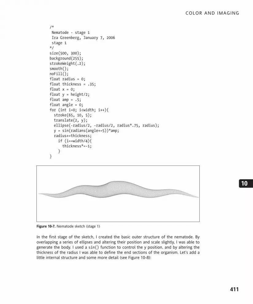
/*Nematode - stage 1Ira Greenberg, January 7, 2006stage 1*/size(500, 300);background(255);strokeWeight(.2);smooth();noFill();float radius = 0;float thickness = .35;float x = 0;float y = height/2;float amp = .5;float angle = 0;for (int i=0; i<width; i++){stroke(65, 10, 5);translate(2, y);ellipse(-radius/2, -radius/2, radius*.75, radius);y = sin(radians(angle+=5))*amp;radius+=thickness;if (i==width/4){thickness*=-1;
}}
Figure 10-7. Nematode sketch (stage 1)
In the first stage of the sketch, I created the basic outer structure of the nematode. Byoverlapping a series of ellipses and altering their position and scale slightly, I was able togenerate the body. I used a sin() function to control the y position, and by altering thethickness of the radius I was able to define the end sections of the organism. Let’s add alittle internal structure and some more detail (see Figure 10-8):
COLOR AND IMAGING
411
10
617xCH10.qxd 4/17/07 1:34 PM Page 411

/*Nematode - stage 2Ira Greenberg, January 7, 2006*/size(500, 300);background(255);strokeWeight(.2);smooth();noFill();float radius = 0;float thickness = .35;float x = 0;float y = height/2;float amp = .5;float angle = 0;float angle2 = 0;for (int i=0; i<width/2-15; i++){stroke(65, 10, 5);noFill();translate(2, y);if (i >= width/2-40) {fill(195, 110, 105, 70);
}else if (i >= width/4-40 && i <= width/2-100){fill(195, 110, 105, 8);
}else {fill(195, 110, 105, 2);
}ellipse(-radius/2, -radius/2, radius*.75, radius);noStroke();fill(205, 110, 105, 40);ellipse(-radius/2, -radius/2, radius*.25, radius*.25);fill(205, 110, 105, 200);ellipse(-radius/2, -radius/2, radius*.05, radius*.05);y = sin(radians(angle+=5))*amp;radius+=thickness;radius+=sin(radians(angle2+=random(30)))*.4;if (i==width/4){thickness*=-.9;
}}
PROCESSING: CREATIVE CODING AND COMPUTATIONAL ART
412
617xCH10.qxd 4/17/07 1:34 PM Page 412

Figure 10-8. Nematode sketch (stage 2)
In this stage, I mostly just added some more ellipses, controlling their radii and color/alpha.I also added a sin() function, with random amplitude to add some jitter to the nema-tode’s body. I think nematodes are actually pretty smooth, but I’ll invoke artistic licensehere. Here’s a finished nematode (see Figure 10-9):
/*Finished NematodeIra Greenberg, January 7, 2006*/void setup(){size(500, 300);background(255);smooth();strokeWeight(.2);noFill();float radius = 0;float thickness = .35;float x = 0;float y = height/2;float amp = .5;float angle = 0;float angle2 = 0;
//ground planestroke(150, 100, 20);line(0,50, width, 50);
for (int i=0; i<width/2-15; i++){noFill();translate(2, y);// add some surface shadingif (i >= width/2-40) {fill(195, 110, 105, 50);
}else if (i >= width/4-40 && i <= width/2-100){fill(195, 110, 105, 10);
COLOR AND IMAGING
413
10
617xCH10.qxd 4/17/07 1:34 PM Page 413

}else {fill(195, 110, 105, 2);
}//outer shell 1stroke(145, 10, 5, 175);ellipse(-radius/2, -radius/2, radius*.75, radius);
//outer shell 2stroke(65, 10, 100, 150);ellipse(-radius/2, -radius/2, radius*.71, radius*.71);
// organs 1stroke(200, 200, 30, i*.8);ellipse(-radius/2, -radius/2, segment(radius, angle), "
segment(radius, angle));
// organs 2noStroke();fill(150, 75, 100, 28);ellipse(-radius/2, -radius/2, segment(radius*.7, angle), "
segment(radius*.7, angle));
// inner tubefill(205, 110, 105, 40);ellipse(-radius/2, -radius/2, radius*.25, radius*.25);
// inner veinfill(205, 110, 105, 200);ellipse(-radius/2, -radius/2, radius*.05, radius*.05);y = sin(radians(angle+=5))*amp;radius+=thickness;radius+=sin(radians(angle2+=random(30)))*.4;if (i==width/4){thickness*=-.9;
}}
}
float segment(float rad, float angle){if(rad>25){rad*=1.5+random(.15);
}else{rad*=random(.2);
}float r = cos(radians(angle*=1.3))*rad*.5;return r;
}
PROCESSING: CREATIVE CODING AND COMPUTATIONAL ART
414
617xCH10.qxd 4/17/07 1:34 PM Page 414

Figure 10-9. Finished Nematode sketch
There’s so much more that could be done with the nematode, but I’ll leave that to you.However, I’ll include one more nematode image, shown in Figure 10-10, on a dark back-ground with some minor changes to a few of the stroke values. Since the nematode imageis translucent, when you add a dark background, the image takes on an interesting lookand feel, resembling a film negative or X-ray.
Figure 10-10. Finished Inverted Nematode sketch
Setting the color modeSo far, this chapter has been using the fill() and stroke() functions with the defaultRGB color mode. Using this mode, each of the R, G, and B color components can beassigned an int or float value from 0 to 255. However, Processing has an alternative HSBcolor mode, which can be set by calling colorMode(HSB). HSB stands for hue, saturation,and brightness. These components correlate to the three color properties of hue, chro-matic intensity, and value, which I discussed earlier in the “Color theory” section of thechapter. By default, RGB and HSB modes use a value range of 0 to 255 for each ofthe three components. In the next example, I create the six primary and secondary colorsand cyan using both modes (see Figure 10-11):
COLOR AND IMAGING
415
10
617xCH10.qxd 4/17/07 1:34 PM Page 415

// Color Modes RGB/HSBsize(400, 114);smooth();color red1 = color(255, 0, 0);color orange1 = color(255, 127, 0);color yellow1 = color(255, 255, 0);color green1 = color(0, 255, 0);color cyan1 = color(0, 255, 255);color blue1 = color(0, 0, 255);color purple1 = color(255, 0, 255);
colorMode(HSB);color red2 = color(0, 255, 255);color orange2 = color(21.25, 255, 255);color yellow2 = color(42.5, 255, 255);color green2 = color(85, 255, 255);color cyan2 = color(127.5, 255, 255);color blue2 = color(170.0, 255, 255);color purple2 = color(212.5, 255, 255);
color[][]cols = { "{ red1, orange1, yellow1, green1, cyan1, blue1, purple1 }, { red2, orange2, yellow2, green2, cyan2, blue2, purple2 }
};
int w = width/cols[0].length;int h = w;for (int i=0; i<2; i++){for (int j=0; j<cols[i].length; j++){fill(cols[i][j]);rect(w*j, h*i, w, h);}
}
Figure 10-11. Color Modes RGB/HSB sketch
If you look carefully at the HSB section in the last example, you’ll notice that, with theexception of orange2, all the colors represent an increase of 42.5. 42.5 is equal to 255divided by 6. This progression in color from red to purple follows the same color order as
PROCESSING: CREATIVE CODING AND COMPUTATIONAL ART
416
617xCH10.qxd 4/17/07 1:34 PM Page 416

the decreasing wavelengths of the individual colors forming the visible light spectrum—the small fraction of the total electromagnetic spectrum our eyes can see. Red’s wave-length is approximately 700 nanometers (nm), and violet’s is around 400 nm. Perhaps youremember roy g biv (red, orange, yellow, green, blue, indigo, violet), a mnemonic many ofus learned to remember the colors in the rainbow. Following is a simple sketch thatcreates a smooth color gradient across the visual spectrum (see Figure 10-12):
// ROY G BIVsize(400, 120);noStroke();colorMode(HSB);float w = width/(255-42.5);for (int i=0; i<width; i+=w){fill(i, 255, 255);rect(w*i, 0, w, height);
}
Figure 10-12. ROY G BIV sketch
There are times when it would be more convenient to use a different range than 0 to 255to control the color components. In the last example, I was forced to do a little math tofigure out the ratio of the width of the display window to the range of color values, in theline float w = width/(255-42.5);. I don’t mean to be lazy, but it would have been easierto simply specify the range of color from 0 to the display window width and let thecalculation-loving computer deal with the crunching. Happily, Processing includes a simpleway to do just that. The colorMode() function has some optional arguments for setting arange of color values. For example, here’s a math-lite version of the last sketch.
// ROY G BIV// math-lite versionsize(400, 120);noStroke();colorMode(HSB, width);for (int i=0; i<width; i++){fill(i, width, width);rect(i, 0, i, height);
}
COLOR AND IMAGING
417
10
617xCH10.qxd 4/17/07 1:34 PM Page 417

This sketch is not a pure copy, as there is some extra red at the end of the spectrum. Toremove this, I’d still need to deal with the extra one-sixth of color range—which means I’mback to doing a little math—so I’ll tolerate the extra pretty red on the right. Not only canyou specify the overall range, you can do it per component, and the ranges you assign toeach component can be bizarrely different. Here’s a rather silly example illustrating this(see Figure 10-13):
// Multi Modessize(720, 100);noStroke();// standard valuescolorMode(HSB, 360, 100, 100);for (int i=0; i<360; i++){for (int j=0; j<100; j++){fill(i, j, j);rect(i, j, 1, 1);
}}
// ridiculous, but possiblecolorMode(HSB, 1.0, .01, 3000);for (float i=0, ii=0; i<1.0; i+=1.0/360.0, ii++){for (float j=0, jj=0, k=0; j<.01; j+=.01/100.0, "
jj++, k+=3000.0/100.0){fill(i, j, k);rect(360+ii, jj, 1, 1);
}}strokeWeight(2);stroke(0);noFill();rect(0, 0, 360, 100);rect(360, 0, 360, 100);
Figure 10-13. Multi Modes sketch
The first gradient was generated using 360, 100, and 100 as the ranges for the H, S, and Bcomponents, respectively. This is actually a standard way for representing HSB, where 360represents the degrees around the color circle and the two 100s represent 100 percentsaturation and 100 percent brightness. I then created an identical gradient using bizarre
PROCESSING: CREATIVE CODING AND COMPUTATIONAL ART
418
617xCH10.qxd 4/17/07 1:34 PM Page 418

values, just to illustrate the possibility. This second nested for loop is pretty frighteninglooking, so don’t give yourself a hard time if you don’t feel like unraveling it. You can alsospecify individual component color ranges for RGB mode, again specifying one or threeoptional arguments when calling the colorMode(RGB) function; I’ll leave that for you to tryon your own.
More convenient color functions Before moving on to imaging, I want to look at some more convenient color functionsincluded in Processing. For creating quick, easy color blends, Processing includes twofunctions: blendColor() and lerpColor(). Here’s a blendColor() example, shown inFigure 10-14:
//blendColorsize(400, 400);smooth();noStroke();color c1 = color(255, 127, 0);color c2 = color(0, 75, 150);
color[] blends = { blendColor(c1, c2, ADD), /*tan*/blendColor(c1, c2, SUBTRACT), /*red*/blendColor(c1, c2, DARKEST), /*green*/blendColor(c1, c2, LIGHTEST) /*pink*/
};
// backgroundfill(c1);rect(0, 0, width, height);
for (int i=0; i<4; i++){fill(blends[i]);arc(width/2, height/2, width/1.25, height/1.25, "
PI/2*i, PI/2*i+PI/2);}
// front circlefill(c2);arc(width/2, height/2, width/4, height/4, 0, TWO_PI);
COLOR AND IMAGING
419
10
617xCH10.qxd 4/17/07 1:34 PM Page 419

Figure 10-14. blendColor() sketch
blendColor() takes two colors as arguments and a third mode argument that controlshow the two colors are blended. The different modes are BLEND, ADD, SUBTRACT, DARKEST,and LIGHTEST. The underlying math behind each of these modes is a little complicated—I’ll look at that a bit later in the chapter when I discuss imaging, which includes a similarblending function. (Please note that as of this writing, BLEND mode, which I did not includein the example, requires the second color argument in the blendColor() call to have analpha setting below 255, or no apparent blend will be detectable.)
An alternative to blendColor() is lerpColor(). The lerp part of the function name refersto linear interpolation. Interpolation just means finding values between other discretevalues. Processing actually includes a math function called lerp() that does just this.Here’s a lerp() example:
// lerp()int a = 1;int b = 2;int steps = 5;float interpolationValue = 1.0/steps;for (int i=1; i<steps; i++){println(lerp(a, b, interpolationValue*i));
}
This example outputs the values 1.2, 1.4, 1.6, and 1.8. lerp() requires three arguments: thetwo discrete values to interpolate between and an interpolation value (a percentageexpressed as a value between 0 and 1.0). For example, to find a value midway between twonumbers, you’d use an interpolation value of .5. A more useful and common application ofinterpolation in computer graphics is for finding points along a path.
PROCESSING: CREATIVE CODING AND COMPUTATIONAL ART
420
617xCH10.qxd 4/17/07 1:34 PM Page 420

lerpColor() uses the same approach as lerp(), but applies it to blending colors. It alsorequires three arguments: two colors and an interpolation value. Here’s a lerpColor()example (see Figure 10-15):
// lerpColor()size(400, 400);noStroke();color c1 = color(255, 255, 0);color c2 = color(150, 0, 150);
// change these values to alter gradientfloat stepsH = 16;float stepsW = 16;
/* ratio to remap any number ofcells into 0 - 1.0 range forlerpColor interpolation argument */float remapFactor = 100.0/(stepsH*stepsW);
float cellW = width/stepsW;float cellH = height/stepsH;int cellCounter = 0;
for (int i=0; i<stepsH; i++){for (int j=0; j<stepsW; j++){fill(lerpColor(c1, c2, (remapFactor*cellCounter)*.01));rect(j*cellW, i*cellH, cellW, cellH);cellCounter++;
}}
Figure 10-15. lerpColor() sketch
COLOR AND IMAGING
421
10
617xCH10.qxd 4/17/07 1:34 PM Page 421

I used a changing interpolation value in the last example to create a gradient blendbetween the two color arguments through the display window. Try changing the startingcolor values as well as the variables stepsH and stepsW (which can be different from oneanother) to alter the color gradient.
In addition to blendColor() and lerpColor(), Processing includes seven other handyfunctions for accessing individual color component values. I’ve included six of these func-tions within the next example, which outputs the individual color components (R, G, andB) as well as hue, saturation, and brightness values; I didn’t include alpha(), but it workssimilarly to the other six (the sketch output can be seen in Figure 10-16):
// Color Component Functionscolor c1 = color(123, 200, 52);println("Default RGB, 255");println("red = "+ red(c1));println("green = "+ green(c1));println("blue = "+ blue(c1));println("hue = "+ hue(c1));println("saturation = "+ saturation(c1));println("brightness = "+ brightness(c1));
println("\nStandard HSB 360, 100, 100");colorMode(HSB, 360, 100, 100);println("red = "+ red(c1));println("green = "+ green(c1));println("blue = "+ blue(c1));println("hue = "+ hue(c1));println("saturation = "+ saturation(c1));println("brightness = "+ brightness(c1));
println("\nAlternative RGB 1.0");colorMode(RGB, 1.0);println("red = "+ red(c1));println("green = "+ green(c1));println("blue = "+ blue(c1));println("hue = "+ hue(c1));println("saturation = "+ saturation(c1));println("brightness = "+ brightness(c1));
PROCESSING: CREATIVE CODING AND COMPUTATIONAL ART
422
617xCH10.qxd 4/17/07 1:34 PM Page 422

I want to mention two final points about using these functions. First, according to theProcessing API reference, these functions are somewhat slow—say, for extracting compo-nent data from many colors at a time. The reference suggests using bitwise operations ifspeed is an issue. I cover bitwise operations in detail in Appendix B, and I also look at someexamples that utilize them a little later in this chapter. Second, these seven functionsreturn a float value, regardless of whether you originally specified int values when youcreated the color. So, for example, if you created a color using the default RGB mode (e.g.,color c = color(200, 150, 74)) and you then called red(c), the value returned wouldbe 200.0, not 200. I know it’s just a 0 after the dot, but this could cause problems if youtried to assign the returned value to a variable declared as type int. Try running the fol-lowing three lines; you should get a compiler error:
//generates a compiler errorcolor c = color(200, 134, 119);int r = red(c);
ImagingThus far in the book, I’ve been utilizing a vector graphics approach, in which images arecreated and manipulated using mathematical expressions that plot a shape and apply ren-dering attributes, such as stroke weight, fill color, corner joins, and so on. Processing hasthe ability to work deeper, down at the pixel or raster level. In a sense, you’ve been gettingnear the pixel level when you used 1 ! 1 pixel rectangles to create some gradients.However, using rectangles to represent pixels is a very inefficient way to approach imaging.In addition, most people connect photo manipulation with imaging, which you’d be hard-pressed to do with a series of rect() calls.
Figure 10-16. Color Component Functions sketch
COLOR AND IMAGING
423
10
617xCH10.qxd 4/17/07 1:34 PM Page 423

GradientsI’ll begin with some simple pixel gradients and then play with some images. This firstsketch, shown in Figure 10-17, creates a linear gradient and utilizes Processing’s set()function. This function allows me to change the color of a pixel, as well as load an imageinto the display window. For now, I’ll just show you how to change some pixels. The func-tion expects three arguments: set(x, y, color).
// Simple Linear Gradient// January 12, 2006// x and y axis
// constantsint Y_AXIS = 1;int X_AXIS = 2;
void setup(){size(400, 400);
// create some gradients// backgroundcolor b1 = color(190, 190, 190);color b2 = color(20, 20, 20);setGradient(0, 0, width, height, b1, b2, Y_AXIS);//center squarescolor c1 = color(255, 120, 0);color c2 = color(10, 45, 255);color c3 = color(10, 255, 15);color c4 = color(125, 2, 140);color c5 = color(255, 255, 0);color c6 = color(25, 255, 200);setGradient(50, 50, 150, 150, c1, c2, Y_AXIS);setGradient(200, 50, 150, 150, c3, c4, X_AXIS);setGradient(50, 200, 150, 150, c2, c5, X_AXIS);setGradient(200, 200, 150, 150, c4, c6, Y_AXIS);
}
void setGradient(int x, int y, float w, float h, "color c1, color c2, int axis ){
// calculate differences between color components float deltaR = red(c2)-red(c1);float deltaG = green(c2)-green(c1);float deltaB = blue(c2)-blue(c1);
// choose axisif(axis == Y_AXIS){/*nested for loops set pixelsin a basic table structure */
PROCESSING: CREATIVE CODING AND COMPUTATIONAL ART
424
617xCH10.qxd 4/17/07 1:34 PM Page 424

// columnfor (int i=x; i<=(x+w); i++){// rowfor (int j=y; j<=(y+h); j++){color c = color( "
(red(c1)+(j-y)*(deltaR/h)), "(green(c1)+(j-y)*(deltaG/h)), "(blue(c1)+(j-y)*(deltaB/h)) );
set(i, j, c);}
}}else if(axis == X_AXIS){// column for (int i=y; i<=(y+h); i++){// rowfor (int j=x; j<=(x+w); j++){color c = color( "
(red(c1)+(j-x)*(deltaR/h)), "(green(c1)+(j-x)*(deltaG/h)), "(blue(c1)+(j-x)*(deltaB/h)) );
set(j, i, c);}
}}
}
Figure 10-17. Simple Linear Gradient sketch
COLOR AND IMAGING
425
10
617xCH10.qxd 4/17/07 1:34 PM Page 425

The Simple Linear Gradient example uses a custom setGradient() function that allowsyou to specify the size, position, colors, and axis of the gradient within the display window.The nested for loops in the function may look a little confusing. The math stuff is simplerthan it looks. Initially in the function, the three local variables deltaR, deltaG, and deltaBare assigned the differences between the R, G, and B components, respectively, within thetwo colors. The rest of the problem involves iterating each component from color c1 tocolor c2 evenly in the for loops. By dividing the delta values by the axis dimension, I getthe ratio of the delta to the height, which I then multiply by the counter j. This way, eventhough j is incremented by 1 in the loop, the ratio will translate to the appropriate valuefor the color component, creating a smooth, continuous gradient. Also, the reason I sub-tract the y and x from j in both loop options is to ensure that the beginning of the gradi-ent begins with c1, not c1 plus the value of x or y. As always, play with this sketch andchange things. I also recommend calling some println() commands and checking on thevalues of variables during the for loops. When I debug my programs (which takes up toomuch of my time), I am constantly calling println() with a variable name as an argumentto see how the program is working.
Next, I’ll create the radial gradient shown in Figure 10-18. (Please be patient—this sketchcan take some time to render.)
// Simple Radial Gradient// January 12, 2006void setup(){size(400, 400);background(0);smooth();
// create a simple table of gradientsint columns = 4;int radius = (width/columns)/2;// create some gradientsfor (int i=radius; i<width; i+=radius*2){for (int j=radius; j<height; j+=radius*2){createGradient(i, j, radius, "color(int(random(255)), int(random(255)), int(random(255))), "color(int(random(255)), int(random(255)), int(random(255))));
}}
}
void createGradient (float x, float y, float radius, "color c1, color c2){
float px = 0, py = 0, angle = 0;
// calculate differences between color components float deltaR = red(c2)-red(c1);float deltaG = green(c2)-green(c1);float deltaB = blue(c2)-blue(c1);// hack to ensure there are no holes in gradient
PROCESSING: CREATIVE CODING AND COMPUTATIONAL ART
426
617xCH10.qxd 4/17/07 1:34 PM Page 426

// needs to be increased, as radius increasesfloat gapFiller = 8.0;
for (int i=0; i<radius; i++){for (float j=0; j<360; j+=1.0/gapFiller){px = x+cos(radians(angle))*i;py = y+sin(radians(angle))*i;angle+=1.0/gapFiller;color c = color( "
(red(c1)+(i)*(deltaR/radius)), "(green(c1)+(i)*(deltaG/radius)), "(blue(c1)+(i)*(deltaB/radius)) );
set(int(px), int(py), c);}
}// adds smooth edge // hack anti-aliasingnoFill();strokeWeight(3);ellipse(x, y, radius*2, radius*2);
}
Figure 10-18. Simple Radial Gradient sketch
COLOR AND IMAGING
427
10
617xCH10.qxd 4/17/07 1:34 PM Page 427

The radial gradient functions similarly to the linear one, except I used some trig func-tions. The way it works is that the radius keeps increasing each iteration of the outer forloop. The nested loop creates a circle of colored pixels at each radius length. A blendoccurs between color 1 and color 2, as it did in the linear example. I had to add someminor “hacks,” however. Since the set() function only takes ints, not floats, I needed toexplicitly convert the px and py variables to ints with the calls int(px) and int(py). Inaddition, as the pixels were drawn around each circle at the respective radii lengths, Inoticed some small (and annoying) gaps in the gradient. To compensate, I created thegapFiller variable, which ensures that extra pixels are drawn to fill in the gaps. I lookforward to hearing from one of you on how to more elegantly solve this problem—fullbragging rights extended.
Before moving on to another approach to writing pixels, let’s look at one more less “regu-lar” example. This example, shown in Figure 10-19, also takes some time to render.
/*Wave GradientJanuary 13, 2006*/size(600, 400);background(200,200,200);float angle = 0;float px = 0, py = 0;float amplitude = 30;float frequency = 0;float fillGap = 2.5;color c;
for (int i=-50; i<height+50; i++){// reset angle to 0, so waves stack properlyangle = 0;// increasing frequency causes more gapsfrequency+=.003;for (float j=0; j<width+50; j++){py = i+sin(radians(angle))*amplitude;angle+=frequency;c = color( "
abs(py-i)*255/amplitude, "255-abs(py-i)*255/amplitude, "j*(255.0/(width+50)) );
// hack to fill gaps. Raise value of fillGap// if you increase frequencyfor (int filler=0; filler<fillGap; filler++){set(int(j-filler), int(py)-filler, c);set(int(j), int(py), c);set(int(j+filler), int(py)+filler, c);
}}
}
PROCESSING: CREATIVE CODING AND COMPUTATIONAL ART
428
617xCH10.qxd 4/17/07 1:34 PM Page 428

Figure 10-19. Wave Gradient sketch
Hopefully this last sketch didn’t cook your computer. Between the two nested loops,there’s a fair amount of processing. The gradient is determined by a simple sine wave withincreasing frequency; this is what gives the gradient its asymmetry. The color is deter-mined, somewhat arbitrarily, by some simple expressions. The red component is generatedby the sine function, the green component is based on 255 (minus the value of the sinefunction), and the blue component is determined by the counter j. In all three cases, thecomponent color values calculated by the expressions are remapped to a range of 0 to255. Definitely mess around with some of the values, especially the color expressions andthe frequency. At the bottom of the function, the third for loop fills gaps in the gradient,similarly to what was done in the radial gradient sketch. You can also try changing thefillGap variable to see what happens. Using the set() function is relatively straightfor-ward, but not the fastest way to change pixel data in Processing.
Faster pixel functionsThere are three other language structures (two functions and an array) that can speedthings up. The three structures are loadPixels(), updatePixels(), and pixels[]. Thefirst structure, loadPixels(), creates an array of pixels (assigned to the built-in global vari-able pixels[]) of the entire display window. The number of pixels in the display windowcan be calculated by width * height. So, for example, a 400 ! 400 display would equal160,000 pixels. Here’s some evidence:
size(400, 400);loadPixels();print(pixels.length);
COLOR AND IMAGING
429
10
617xCH10.qxd 4/17/07 1:34 PM Page 429

The pixels[] array stores each pixel as Processing’s color data type, structured in consec-utive rows. For example, if the sketch size is 100 ! 100, then the 5,050th pixel(pixels[5049]) will be close to the center point in the display window. Here’s an examplethat directly changes the color of that pixel:
size(100, 100);background(0);loadPixels();pixels[5050] = color(255);updatePixels();
The Processing reference includes a very simple mathematical expression to help you tar-get a pixel in the pixels[] array of the display window: pixels[y*width+x]. Based on thisexpression, the last little sketch (shown in Figure 10-20) could be rewritten as follows:
size(100, 100);background(0);loadPixels();pixels[height/2*width+width/2] = color(255);updatePixels();
Figure 10-20. Pixels array (single white pixel) sketch
To change more than 1 pixel, a loop will help. The next example divides the display win-dow in horizontal bands, assigning a different color to each band (see Figure 10-21):
// Color Banding with pixels[]size(400, 400);loadPixels();int px = pixels.length;int bands = 20; // should be a factor of pxcolor c;
PROCESSING: CREATIVE CODING AND COMPUTATIONAL ART
430
617xCH10.qxd 4/17/07 1:34 PM Page 430

for (int i=0; i<bands; i++){c = color(random(255), random(255), random(255));for (int j=(px/bands)*i; j<px/bands*(i+1); j++){pixels[j] = c;
}}updatePixels();
Figure 10-21. Color Banding with pixels[] sketch
You need to call loadPixels() prior to utilizing the pixels[] array. If you neglect to callloadPixels(), you’ll get a null pointer error, which essentially means that you’re trying toaccess something that hasn’t been created yet. After you make any changes to pixels[],you’ll need to call updatePixels() to see your changes updated in the display window. Ifyou don’t call the function, you’ll neither get an error message nor see your updates.These types of (annoying) errors are categorized as “failing silently,” which can be a royalpain when debugging.
In the last sketch, I created the variable px to hold the length value of pixels[]. I did thisjust for convenience, as px was shorter to write than pixels.length. Every array has a pub-lic length property that is especially useful when setting the limit of a loop. For example, torandomly assign a color to every pixel on the screen, I could do this (see Figure 10-22):
// Color Staticsize(400, 400);loadPixels();int px = pixels.length;color c;for (int i=0; i<px; i++){c = color(random(255), random(255), random(255));pixels[i] = c;
}updatePixels();
COLOR AND IMAGING
431
10
617xCH10.qxd 4/17/07 1:34 PM Page 431

Figure 10-22. Color Static sketch
Image manipulationAs you might suspect, the pixels[] array has better uses than creating static.loadPixels() collects all the pixels in the window, regardless of whether the pixels makeup a single color background fill or a photographic image. The more interesting latter caseopens the door to all kinds of imaging possibilities. However, before looking at the nextsketch, let’s review how to load an image.
To work with images in Processing, you need to load them into a data directory thatresides within the current sketch directory. It’s a very simple process. Under Sketch in thetop menu bar, select the Add File command. This command opens a file browser, allowingyou to select an image to copy into the data directory. If there isn’t a data directory,Processing will automatically create one for you. If you eventually make additional changesto the image using a program like Photoshop, you’ll need to remember to add the alteredimage to your data directory again (it’s not updated automatically). One cautionary note:when you add an image into the data directory with the same name as an existing image,the original image will be replaced by the image you add, without any warning. Processingcan work with GIF, JPG, TGA, and PNG images.
The following sketch (shown in Figure 10-23) loads an image (my dog Heidi) into the dis-play window (obviously, you’ll need to change the name heidi.jpg to the image you’reusing):
// Load an Imagesize(600, 400);PImage img1;img1 = loadImage("heidi.jpg");image(img1, 0, 0);
PROCESSING: CREATIVE CODING AND COMPUTATIONAL ART
432
617xCH10.qxd 4/17/07 1:34 PM Page 432

Figure 10-23. Load an Image sketch
Pretty painless, don’t you think? If you did run into a problem, remember that Processingis case sensitive, so .JPG is different than .jpg. In addition, Processing can’t (easily) handlehuge files the way a program like Photoshop can, which can utilize virtual memory (mem-ory borrowed from the hard drive). Also remember that image size and resolution areinterconnected, so just changing the size of the image’s dimensions won’t reduce its mem-ory requirements; it will just increase the resolution of the smaller image.
If you’re working with a very large image and run into the java.lang.OutOfMemoryError,you can try allocating more memory to Processing by selecting Preferences from the topProcessing menu. Make sure that the Set Maximum Available Memory box is selected, andthen try incrementally (and cautiously) raising the value. Processing’s default value is512KB. To learn more about memory issues/errors in Processing, check out http://processing.org/faq/bugs.html#memory.
Notice in the last example that I declared the variable img1 of type PImage. Similarly toProcessing’s color data type, PImage is a unique Processing data type, used to store imagedata. The line img1 = loadImage("heidi.jpg"); in the example creates a PImage object.This line didn’t actually draw the image to the screen, but constructed a PImage objectcontaining the relevant image data.
One of the challenges of loading images or other forms of external data is the latency, ordelay, between the input request and the data actually being loaded into the program. Asyou can imagine, this delay can be substantial for large image files. Using pure Java, load-ing images can be a bit involved, requiring structures for tracking the image data as it’sloading—much lower-level than most of us would want to go. PImage, along with theloadImage() function, encapsulates this entire loading process (thankfully).
COLOR AND IMAGING
433
10
617xCH10.qxd 4/17/07 1:34 PM Page 433

In addition to loadImage(), you can use the image() function to actually draw the imageto the screen, as in the line image(img1, 0, 0);. The second and third arguments in thecall (0, 0) are for the x and y position of the image. Images are positioned from the top-left corner of the image. In the last example, if I had wanted to center the image in the dis-play window (assuming, of course, that the image was smaller than the window), I couldhave used the following:
//load and center an imagesize(700, 500);PImage img1;img1 = loadImage("heidi.jpg");translate(width/2, height/2);image(img1, -img1.width/2, -img1.height/2);
Since PImage is a data type (think class), it includes properties (also referred to as fields)and methods. PImage objects have width and height properties, which I conveniently usedin calculating the image position (centered). More information about the PImage data type,including its other fields/methods, can be found at http://processing.org/reference/PImage.html.
In the last example, I called the image() function to display my image. set() can also becalled to load images—in this case, two copies of the same image—the same functioncalled earlier to change the color of a pixel (see Figure 10-24):
//Loading Images with set()size(600, 400);background(245);PImage img2 = loadImage("kids.jpg");set(50, 50, img2);set(img2.width+100, 50, img2);
Figure 10-24. Loading Images with set() sketch
PROCESSING: CREATIVE CODING AND COMPUTATIONAL ART
434
617xCH10.qxd 4/17/07 1:34 PM Page 434

The image() function has an extra feature that I think makes it more useful than set() forloading images: the ability to resize the image as you load it. The next example, shown inFigure 10-25, tiles images in the display window using image(img, x, y, w, h). I recom-mend using an image approximately 400 (width) ! 300 pixels to try the example.
//Image Tilingsize(650, 450);PImage img2 = loadImage("heidi.jpg");int cols = 8;int rows = 8;int w = width/cols;int h = height/rows;for (int i=0; i<height; i+=h){for (int j=0; j<width; j+=w){image(img2, j, i, w, h);
}}
Figure 10-25. Image Tiling sketch
COLOR AND IMAGING
435
10
617xCH10.qxd 4/17/07 1:34 PM Page 435

Besides the set() function, it’s probably no surprise that there’s also a get() function.get() can return the color of a single pixel, an entire PImage, or a section of a PImage. Thislast case can be useful for creating a collage of image fragments (if that’s the sort of thingyou enjoy doing). Here’s an example, shown in Figure 10-26, that copies four pieces of theimage and pastes them in a stack on the right side of the display window. Please note thatyour image needs to be 650 (width) ! 450 pixels for this example to render properly.
//Compositingsize(650, 450);PImage img = loadImage("hong_kong.jpg");image(img, 0, 0);int w = width/5;int h = height/5;PImage[]frags = { get(130, 140, w, h),get(475, 220, w, h),get(220, 300, w, h),get(300, 205, w, h),get(100, 250, w, h)};
for (int i=0; i<5; i++){image(frags[i], width-w, h*i);
}
Figure 10-26. Compositing sketch
PROCESSING: CREATIVE CODING AND COMPUTATIONAL ART
436
617xCH10.qxd 4/17/07 1:34 PM Page 436

In the last example, I created an array of anonymous PImages using the get() command.This syntax may look odd, as I’m relying on the returned values of the get() calls (whichare PImages) to populate the arrays. You’ll remember that arrays can be instantiated a fewdifferent ways; one such way is to declare and populate the array at the same time, withthe values specified between curly braces, as illustrated in the example.
A more ambitious but interesting thing to do with get() could be to write your ownimage-encrypting sketch. The simple encryption procedure will collect the image assequential fragments and then re-create the image, reordering the image. I’ll keep it reallysimple and just reverse the order of the fragments. You need to use an image of 600(width) ! 400 pixels to run the example (see Figure 10-27):
//Simple Image Encryptionint ENCRYPTION_LOW = 0;int ENCRYPTION_MEDIUM = 1;int ENCRYPTION_HIGH = 2;int ENCRYPTION_VERY_HIGH = 3;
void setup(){size(600, 400);PImage img = loadImage("changsha.jpg");image(img, 0, 0);
// call the fragment functionfragment(ENCRYPTION_HIGH);
}
void fragment(int encryptionLevel){int fragW = 0;int fragH = 0;int frags = 0;// set size of blocksswitch(encryptionLevel){
case 0:fragW = width/2;fragH = height/2;frags = 4;break;case 1:fragW = width/4;fragH = height/4;frags = 16;
break;case 2:fragW = width/8;fragH = height/8;frags = 64;
break;case 3:
COLOR AND IMAGING
437
10
617xCH10.qxd 4/17/07 1:34 PM Page 437

fragW = width/10;fragH = height/10;frags = 100;
break;}
// fill array with image blocksPImage[]imgs = new PImage[frags];int fragCounter = 0;for (int i=0, ii=0; i<width; i+=fragW, ii++){for (int j=0, jj=0; j<height; j+=fragH, jj++){imgs[fragCounter++] = get(i, j, fragW, fragH);
}}// call encryption functionencrypt(imgs);
}
//encryptvoid encrypt(PImage[]imgs){PImage[]imgs2 = new PImage[imgs.length];for (int i=imgs.length-1; i>=0; i--){// reverse fragment orderimgs2[abs(i-(imgs.length-1))] = imgs[i];
}update(imgs2);
}
// repaint Display windowvoid update(PImage[]imgs){//reset counterint counter = 0;//reassemble imagefor (int i=0; i<width; i+=imgs[0].width){for (int j=0; j<height; j+=imgs[0].height){image(imgs[counter], i, j);counter++;
}}
}
PROCESSING: CREATIVE CODING AND COMPUTATIONAL ART
438
617xCH10.qxd 4/17/07 1:34 PM Page 438

Figure 10-27. Simple Image Encryption sketch
This is actually a pretty dopey encryption, but hopefully it sparks some ideas. Also, theencryption fragmentation is based on the 600 ! 400 format. If you change that, you’lllikely get an “array out of bounds” error. The basic encryption works by cutting the imageinto fragments that are used to create an array of PImages of all the fragments. At thatpoint, you could write any sorting algorithm you’d like to encrypt (reorder) the fragments.I simply reversed the order with the following expression:
imgs2[abs(i-(imgs.length-1))] = imgs[i];
The function abs() always returns a positive value, allowing me to load the image frag-ments in imgs[] in reverse order into imgs2[]. Upon reviewing the code, If you havetrouble seeing why this works, run the following line in the for loop within the encryptfunction:
println("i = "+i+", abs(i-(imgs.length-1)) = " + "abs(i-(imgs.length-1)));
One minor caution—if you’re on an older computer (sorry), be careful running theVERY_HIGH option, it might take a while.
If you’ve been looking through the imaging section of the Processing reference, you mayhave found some commands with duplicate names. For example, if you click on thePImage link, you’ll see that a number of the method names are the same as functionnames grouped under the Pixels heading in the language reference. The commands areactually different, although functionally they do some similar things. Here’s how to keepthis stuff all straight.
COLOR AND IMAGING
439
10
617xCH10.qxd 4/17/07 1:34 PM Page 439

Display window functionsThe commands grouped under the Pixels heading of the language reference are functionsthat affect the pixels in the display window, regardless of whether those pixels make up abackground color or an image. The pixels[] array specified under this heading is thearray that holds all the pixels making up the display window (again, regardless of what’sin it).
PImage methodsThe PImage data type also has a pixels[] array property that is assigned the pixels makingup the created PImage object. When invoking a method of the PImage class, you use aPImage object reference attached to the property or method with dot syntax. For example,to set a pixel of a PImage named img, you would write img.set(). In contrast, to set a pixelin the display window, you would just use set(). The situation can seem even more con-fusing once img (the PImage object) is drawn to the screen. At that point, the image databecomes part of the display window, which gets collected in the window’s pixels[] array.However, img still retains its original pixel data in memory (in its own img.pixels[] array).
The next sketch, shown in Figure 10-28, uses the PImage method get() to create a pixi-lated image. The variable detail allows you to change the level of pixilation. The originalPImage is never drawn to the screen, but rather the internal image is used for picking colorvalues with the PImage get() method. The picked color values are then used to create amatrix of colored rectangles approximating the image. If you bring the level of detail downto (or near) 1, the colored rectangles will approximate a continuous tone image; you’ll alsowant to uncomment the line //noStroke();. I recommend using an image the same sizeas the display window.
//Pixilatesize(600, 400);PImage img = loadImage("changsha.jpg");//noStroke();int detail = 10;for ( int i=0; i<width; i+=detail){for ( int j=0; j<height; j+=detail){color c = img.get(i, j);fill(c);rect(i, j, detail, detail);
}}
PROCESSING: CREATIVE CODING AND COMPUTATIONAL ART
440
617xCH10.qxd 4/17/07 1:34 PM Page 440

Figure 10-28. Pixilate sketch
The next sketch loads two copies of an image into the display window and increases theright image’s red saturation. Remember, the loadPixels() function call collects the dis-play window pixel data, assigning it to the display window pixels[] array (not theimg.pixels[] array). After making some changes to the pixels[] array, I need to callupdatePixels() to have the changes actually updated within the display window. In theexample, I’m using a 400 ! 400 pixel image and an 800 ! 400 pixel display window (seeFigure 10-29):
//Red Saturationsize(800, 400);PImage img = loadImage("hong_kong.jpg");image(img, 0, 0);image(img, width/2, 0);int threshold = 125;loadPixels();for(int j=0; j<height; j++){for(int i=(width/2+j*width); i<width+j*width; i++){if (red(pixels[i])>threshold){pixels[i] = color(255, green(pixels[i]), blue(pixels[i]));
}}
}updatePixels();
COLOR AND IMAGING
441
10
617xCH10.qxd 4/17/07 1:34 PM Page 441

Figure 10-29. Red Saturation sketch
An easier way to add a tint or color overlay to an image is to use Processing’s tint() func-tion. The function requires a color argument, which can be specified five different ways:gray, with or without alpha; RGB or RGBA color; or a single color value, using Processing’scolor data type. In the next example, shown in Figure 10-30, I used an image the same sizeas the display window (600 ! 400 pixels):
// Tint()size(600, 400);PImage img = loadImage("highway.jpg");image(img, 0, 0);int tintAlpha = 255;
int[][]cols = {{255, 0, 0, tintAlpha}, {255, 255, 0, tintAlpha},{0, 0, 255, tintAlpha}, {0, 255, 0, tintAlpha},{255, 0, 255, tintAlpha}, {255, 127, 0, tintAlpha}
};
int columns = 3;int w = width/columns;int h = cols.length;
for (int i=0; i<h; i++){tintAlpha = 255;for (int j=0; j<w; j++){tint(color(cols[i][0], cols[i][1], cols[i][2], tintAlpha)); image(img, j*w, i*height/h, w, height/h );tintAlpha-=(255/columns);
}}
PROCESSING: CREATIVE CODING AND COMPUTATIONAL ART
442
617xCH10.qxd 4/17/07 1:34 PM Page 442

Figure 10-30. Tint sketch
Speeding things up with bitwise operationsYou might have noticed that this last sketch took some time to render (or maybe yourcomputer is faster than mine). There is a faster, albeit lower-level, way to manipulate theindividual color components packed inside the color data type. The color data type com-bines the individual color components alpha, red, green, and blue into 32 bits of data. Thestructure of the color data type looks like this: AAAAAAAARRRRRRRRGGGGGGGG-BBBBBBBB. Of course, the letters would be replaced by zeros and ones, depending on thecolor specified. For example, run the following sketch to see the bit string for blue:
color c = color(0, 0, 255);println(binary(c));
In the sketch output, the alpha and blue bits are all ones, since I specified maximum valuefor blue (255), and alpha is 255 by default. Likewise, the red and green bits are all zeros,per the original color value I set—color(0, 0, 255).
Bitwise operations allow you to directly manipulate the bits, shifting and even doingsimple mathematical operations on them. Bitwise operations are not for everyone, sodon’t fret if you can’t deal with this approach. However, it’s good to know that the possi-bility exists, and they are quite speedy. I provide a detailed overview of bitwise operationsin Appendix B, so you might want to read that before trying these next few sketches. If,however, you just want to use bitwise operations with a limited understanding of how theyactually work, here’s the highly abridged “recipe” version:
COLOR AND IMAGING
443
10
617xCH10.qxd 4/17/07 1:34 PM Page 443
To access the red, green, blue, and alpha components from a color c, use the followingsyntax:
int a = c >> 24 & 0xFF;int r = c >> 16 & 0xFF;int g = c >> 8 & 0xFF;int b = c & 0xFF;
To combine the individual color components back into a color, use:
// combine components back into a 32-bit integerc = (a << 24) | (r << 16) | (g << 8) | b;
This next sketch combines the two steps, filling the top and bottom of the sketch windowwith a color manipulated using bitwise operations:
// bitwise operationssize(200, 300);noStroke();color c = color(45, 120, 96);
// fill top of windowfill(c);rect(0, 0, width, height/2);
// get color componentsint r = c >> 16 & 0xFF;int g = c >> 8 & 0xFF;int b = c & 0xFF;int a = c >> 24 & 0xFF;
// alter component valuesr += 100;g -= 50;b += 100;
// combine components back into a 32-bit integerc = (a << 24) | (r << 16) | (g << 8) | b;
// fill bottom of windowfill(c);rect(0, height/2, width, height/2);
Here’s an example of tinting an image using bitwise operations (shown in Figure 10-31).I used an image the same size as the display window (600 ! 400 pixels).
PROCESSING: CREATIVE CODING AND COMPUTATIONAL ART
444
617xCH10.qxd 4/17/07 1:34 PM Page 444

/* Tint (using bitwise operations)Created January 18, 2006updated December 4, 2006 */size(600, 400);PImage img = loadImage("changsha2.jpg");PImage img2 = createImage(img.width, img.height, RGB);// copy pixels array from img to img2arraycopy(img.pixels, img2.pixels);int r, g, b, a;int row = height/6;
for(int i=0; i<width*height; i++){// get untinted component valuesr = img2.pixels[i] >> 16 & 0xFF;g = img2.pixels[i] >> 8 & 0xFF;b = img2.pixels[i] & 0xFF;a = img2.pixels[i] >> 24 & 0xFF;
// tint based on height in display windowif (i<width*row){r =255;
} else if (i>width*row && i<width*row*2){r = 255;g = 255;
} else if (i>width*row*2 && i<width*row*3){b = 255;
} else if (i>width*row*3 && i<width*row*4){g = 255;
} else if (i>width*row*4 && i<width*row*5){r = 255;b = 255;
} else {r = 255;g = 127;
}
// combine components back into a 32-bit integerimg2.pixels[i] = (a << 24) | (r << 16) | (g << 8) | b;
}// draw imagesimage(img, 0, 0);image(img2, width/2, 0);
COLOR AND IMAGING
445
10
617xCH10.qxd 4/17/07 1:34 PM Page 445

Figure 10-31. Tint sketch (using bitwise operations)
Again, let me stress the fact that you do not need to use bitwise operations in Processing.The Processing functions red(c), green(c), blue(c), and alpha(c) also return the indi-vidual color component values. However, once you get past the strange bitwise syntax(i.e., >> 16 & 0xFF), you’ll realize they are relatively easy to use, and again, fast.
The last sketch utilized two PImages; the first was created with the line
PImage img = loadImage("changsha2.jpg");
which is the syntax I looked at earlier to create a PImage based on a loaded image. The sec-ond PImage was created with the following line:
PImage img2 = createImage(img.width, img.height, RGB);
This is the syntax to use when you want to create a PImage, but initially only specify its sizeand color format. Notice that I specified the size of the second PImage using the width andheight properties of the first PImage, ensuring that both images were the same size.
As you may remember, every PImage includes a pixels[] array that contains all the colorvalues in the image. Once I created the second PImage, I copied the pixels[] array fromthe first PImage into the second using Processing’s arrayCopy(src, dest) function.
This is a pretty handy function that you need to use to copy arrays. You can’t simply copyan array using syntax like array1 = array2, which only works for primitive types, such asint1 = int2. Arrays and objects are reference types. You may remember from earlier in
PROCESSING: CREATIVE CODING AND COMPUTATIONAL ART
446
617xCH10.qxd 4/17/07 1:34 PM Page 446

the book that a primitive type is directly assigned a specific value (e.g., int i = 1;), but areference type is internally assigned an address in the computer’s memory where theobject is stored. Thus, the syntax array1 = array2 makes the two array variables point tothe same place in the computer’s memory (where the array is stored)—generally not whatyou want to do. This is a fairly advanced topic, but something you do need to be aware of.I cover variables in detail in Chapter 3.
There are a lot of other interesting things you can do using bitwise operations. Here’s asketch, shown in Figure 10-32, that changes the contrast of an image (I used a 400 ! 400pixel image for the example).
/* Contrast (using bitwise operations)created January 18, 2006updated December 4, 2006 */
size(800, 400);PImage img = loadImage("harbor.jpg");PImage img2 = createImage(img.width, img.height, RGB);arraycopy(img.pixels, img2.pixels);
float threshold = 127.5;float contrast = .5; // pos or neg valuesloadPixels();for(int i=0; i<img.width * img.height; i++){// separate out component color valuesint r = img2.pixels[i] >> 16 & 0xFF;int g = img2.pixels[i] >> 8 & 0xFF;int b = img2.pixels[i] & 0xFF;int a = img2.pixels[i] >> 24 & 0xFF;
// redr = int(r*(1.0 + (contrast)*((r-threshold)*.01)));r = constrain(r, 0, 255);
// greeng = int(g*(1.0 + (contrast)*((g-threshold)*.01)));g = constrain(g, 0, 255);
// blueb = int(b*(1.0 + (contrast)*((b-threshold))*.01));b = constrain(b, 0, 255);
// combine components back into a 32-bit integerimg2.pixels[i] = (a << 24) | (r << 16) | (g << 8) | b;
}//draw imagesimage(img, 0, 0);image(img2, width/2, 0);
COLOR AND IMAGING
447
10
617xCH10.qxd 4/17/07 1:34 PM Page 447

Figure 10-32. Contrast sketch (using bitwise operations)
This is a fairly simple contrast implementation that calculates the difference between thecolor component value and some threshold—in this case, the midpoint of the 255-valuecolor range (127.5). This value is multiplied by a contrast value and then added to 1;the color component is then multiplied by this number. So, for example, if the threshold/contrast expression value evaluates to 1.2, and the color component value is 150, it willbecome 180. The reason I subtract the threshold from the component is to generate anice gradient of values so that the contrast shift will be smooth. For example, a color in themid-range (e.g., 129) would be affected very little (multiplied by 1.00225). However, colorsapproaching 0 or 255 would be more intensely affected (e.g., an initial component valueof 240, using .15 as the value of the contrast variable, would become 280.5). The differ-ence in values between the most minimal changes and the most severe would be across agradient proportional to the difference between the component’s original value and thethreshold.
In the example, I was also forced to convert the calculated contrast values from type floatto type int so that I could assign them back to the color component variables, declared astype int. Finally, I used Processing’s constrain() function, which sets a minimum andmaximum for a value. Since my component values needed to stay within the range of 0 to255, I clipped them if they exceeded these limits. With a starting value of 240 and a con-trast value of .15, the calculated value 280.5 would get constrained to 255. You can trycommenting out the constrain() function calls to see what happens when the values dogo out of range; it can be visually interesting. I’ll finish up this section by looking somemore at Processing’s built-in imaging and filtering capabilities.
Imaging filtersProcessing’s PImage class has a method called mask() that allows you to use either animage or a pixel array to mask out part of an image. The mask image should be grayscale.(You can use an RGB image, but only the blue channel of the image will be used as themask.) My suggestion is to convert your mask image to grayscale before using it.
PROCESSING: CREATIVE CODING AND COMPUTATIONAL ART
448
617xCH10.qxd 4/17/07 1:34 PM Page 448

The mask works like an alpha channel. A value of 0 (black) will conceal the image pixel,while a value of 255 (white) will fully reveal the image pixel. Values between 0 and 255 willdisplay the masked pixels in the image with varying degrees of translucency. In the nextsketch, I used one image to mask out the sky area of another image, allowing the displaywindow background color to show through (where the 0 values of the mask pixels are). Imade the sky-shaped mask image from the original image, which I was able to select andconvert using Photoshop. In the two example images, the first image uses a 100 percentblack sky mask, while the second uses a linear gradient from black (top of the sky) to white(bottom of the sky). The two images I used were both 600 ! 480 pixels (see Figures 10-33and 10-34):
// Mask the Skysize(600, 480);background(185, 185, 250);PImage img = loadImage("harbor2.jpg");PImage mask = loadImage("harbor2_mask.jpg");img.mask(mask);image(img, 0, 0, 600, 480);
Figure 10-33. Mask the Sky sketch
COLOR AND IMAGING
449
10
617xCH10.qxd 4/17/07 1:34 PM Page 449

Figure 10-34. Mask the Sky with Gradient sketch
When using a pixel array mask instead of an image, the pixel array size should be the samelength (number of pixels) as the image you’re masking, which means that if your image is600 ! 400, your pixel array should have a length of 240,000 (image width ! image height).Pixel array masks are a very cool feature in Processing that are a little hard to understandat first. Besides providing the ability to create interesting collaged effects, they can also beused to generate a dynamic mask at runtime. In the next example, shown in Figure 10-35,I’ll create a pixel array mask composed of 2,000 random rectangles. The image you useneeds to be the same dimensions as the display window.
// Pixel Array Mask size(600, 400);// set background--the blue channel // contributes to pixel maskbackground(180, 90, 50);
//load but don't display imagePImage img = loadImage("changsha.jpg");
// create a mask composed of rectanglesfill(255);for (int i=0; i<2000; i++){
PROCESSING: CREATIVE CODING AND COMPUTATIONAL ART
450
617xCH10.qxd 4/17/07 1:34 PM Page 450

rect(random(width), random(height), 5+random(15), 5+random(15));}// build pixel array of the screenloadPixels();
// set maskimg.mask(pixels);
//draw imageimage(img, 0, 0, 600, 400);
Figure 10-35. Pixel Array Mask sketch
Since you can collect the pixels in the display window using loadPixels(), you can gener-ate a mask with any of Processing’s drawing functions, which is exactly what I did in thisexample. Using the rect() command, I created 600 rectangles with a fill of 255, and thenI called loadPixels(), which created a pixel array of the image. If you specify an RGB fillvalue, the mask utilizes the value of the blue color component of the pixels. You can alsospecify a grayscale value with a single argument when calling the fill or background func-tion. 0 (black) will be opaque, while 255 (white) will be totally transparent. Values between0 and 255 will have varying translucency. In the example, I set the blue component in thebackground color to 50, giving the pixel mask some overall slight translucency, allowingthe image to show through the background color a little. I gave the rectangles a fill of 255,fully revealing parts of the image through the little rectangle windows. If you’re still notgetting this, try changing some of the values and playing with the code—it’s the best wayto really understand what’s happening.
COLOR AND IMAGING
451
10
617xCH10.qxd 4/17/07 1:34 PM Page 451

blend() and filter()There are two other powerful Photoshop-esque imaging functions in Processing’s toolbox:blend() and filter(). These functions each do so much that they could easily have beendivided into a bunch of separate functions. They’re built upon some very low-levelcoding—mostly using bitwise operations—and were developed as a group effort, withconsiderable contributions by Karsten Schmidt (a.k.a. toxi) (www.toxi.co.uk/) and MarioKlingemann (www.quasimondo.com/). If you’d like to take a look at the actual sourcecode implementation (to better appreciate toxi and Klingemann’s efforts), check outProcessing’s PImage class at http://dev.processing.org/source/index.cgi/trunk/processing/core/src/processing/core/PImage.java?view=markup.
I do, however, have some (small) misgivings about these functions being included inProcessing, as they so deeply encapsulate very low-level processing, and—not unlikePhotoshop—can become easy targets for fast, uninformed effects. In this sense, I feel theirease of use and power actually have the potential to limit creativity. For example, here’s asketch that uses the filter function to invert an image (see Figure 10-36). Please rememberto add an image into your data directory for all the examples prior to using loadImage(),as in the previous examples.
// INVERT Filter// image should be 600 x 400 pixelssize(600, 400);background(255);PImage img = loadImage("view.jpg"); image(img,0,0);filter(INVERT);
Figure 10-36. INVERT Filter sketch
PROCESSING: CREATIVE CODING AND COMPUTATIONAL ART
452
617xCH10.qxd 4/17/07 1:34 PM Page 452

This last sketch couldn’t be simpler. The INVERT argument inverts the pixel color compo-nent values. However, that’s all you can do with it. Now, let’s implement our own custominvert filter. Inverting the color component value is as simple as subtracting 255 from eachcomponent. However, doing that will also generate a negative value or 0. I want positivecolor component values in the range of 0 to 255, so I need to remove the negative sign.Two simple ways to do that would be to multiply each value by –1, or use Processing’sabs() function, which returns the absolute value of the argument.
//custom invert--version 1// image should be 600 x 400 pixelssize(600, 400);background(255);PImage img = loadImage("view.jpg"); image(img, 0, 0);loadPixels();
for (int i=0; i<pixels.length; i++){// separate out and invert component color valuesint r = abs((pixels[i] >> 16 & 0xFF)-255);int g = abs((pixels[i] >> 8 & 0xFF)-255);int b = abs((pixels[i] & 0xFF)-255);int a = pixels[i] >> 24 & 0xFF;
pixels[i] = (a << 24) | (r << 16) | (g << 8) | b;}updatePixels();
This sketch should mimic, in output, the earlier sketch that used Processing’sfilter(INVERT) function. I should also mention that the preceding sketch could be con-densed by using a different bitwise operator, ^, which I believe is how it’s actually inter-nally implemented in Processing. Here’s the condensed, albeit denser, version. I won’tspend more time explaining the bitwise stuff here—but remember that I cover it in detailin Appendix B if you want more info.
//custom invert--version 2// condensed verison// image should be 600 x 400 pixelssize(600, 400);background(255);PImage img = loadImage("view.jpg"); image(img, 0, 0);loadPixels();for (int i=0; i<pixels.length; i++){pixels[i] ^= 0xFFFFFF;
}updatePixels();
COLOR AND IMAGING
453
10
617xCH10.qxd 4/17/07 1:34 PM Page 453

And if you really can’t stand the bitwise stuff, you can also use the color component func-tions, which although not as efficient, get the job done:
//custom invert--version 3// image should be 600 x 400 pixelssize(600, 400);background(255);PImage img = loadImage("view.jpg"); image(img, 0, 0);loadPixels();
for (int i=0; i<(width*height); i++){// separate out and invert component color valuesint r = abs(int(red(pixels[i]))-255);int g = abs(int(green(pixels[i]))-255);int b = abs(int(blue(pixels[i]))-255);int a = int(alpha(pixels[i]));
pixels[i] = color(r, g, b, a);}updatePixels();
So you might ask at this point, “Why would anyone (in their right mind) want to do all thiscustomizing, when you can get the same bang for a whole lot less buck using the prebuiltfunction?” Using Processing’s filter(INVERT) function, you will always get the same con-sistent result. This is not necessarily a bad thing, as it’s convenient to be able to quickly andreliably invert pixels. However, what if, in inverting the pixels, you begin to digressivelywonder (as artists tend to do), “What would happen if, rather than inverting the pixels, Idid something else to them?” A Photoshop user might then go back to the pull-downmenu and look for other cool pre-made effects. However, as a creative coder, I’m notreally looking for a quick answer. Rather, I’m engaged in a search process that hopefullywill to lead to discovering a yet untraveled aesthetic path. When you have a toolbox ofcanned effects, no matter how good, it can be pretty hard to find untrodden territory. Thisis not to imply you should avoid filters. I’m just suggesting taking the time to learn howsome of these effects work programmatically, under the hood. Starting with the custominvert sketch, here’s a variation that creates a smooth gradient between a negative andpositive image. I used a 300 ! 400 pixel photo (of yours truly engaged in rocket science)for this sketch (see Figure 10-37):
// From Neg to Possize(300, 400);background(255);PImage img = loadImage("research.jpg"); image(img, 0, 0);loadPixels();
float invertFactor = 255.0;for (int i=0; i<pixels.length; i++){
PROCESSING: CREATIVE CODING AND COMPUTATIONAL ART
454
617xCH10.qxd 4/17/07 1:34 PM Page 454

// separate out and invert component color valuesfloat r = abs(red(pixels[i])-invertFactor);float g = abs(green(pixels[i])-invertFactor);float b = abs(blue(pixels[i])-invertFactor);// put pixel back togetherpixels[i] = color(r, g, b);
// each row interval decrements invertFactorif (i>0 && i% width==0){invertFactor-=(255.0/height);
}}updatePixels();
Figure 10-37. From Neg to Pos sketch
Besides showcasing a custom invert filter, this last sketch demonstrated another exampleof the usefulness of the modulus operator:
if (i>0 && i% width==0){
By dividing i by the display window width and checking for a 0 remainder, I ensured thatthe variable invertFactor would only be decremented per each row of pixels, giving mea smooth gradation down the image.
COLOR AND IMAGING
455
10
617xCH10.qxd 4/17/07 1:34 PM Page 455

I guess you’ve done enough under-the-hood gazing. Without further interruption, here arethe rest of Processing’s filters and blends, shown in Figures 10-38 through 10-42:
// THRESHOLD Filter// filter(THRESHOLD, float threshold level)// image should be 200 x 200 pixels
size(800, 200);PImage img = loadImage("moonshadow.jpg");float thresholdLevel = 1.0;for (int i=0; i<4; i++){image(img, 200*i, 0, 200, 200);filter(THRESHOLD, thresholdLevel);thresholdLevel-=.25;
}
Figure 10-38. THRESHOLD Filter sketch
The THRESHOLD argument converts the image pixels to black or white depending onwhether their value is below or above a threshold level. The threshold level is between 0.0and 1.0. For example, if the level is .5, then pixels whose values are above 255/2 would beturned white, and those below turned black. The second threshold level argument isoptional; if omitted, Processing uses .5 as the default value. One final subtle point is thatthe value of the pixel is determined by the highest component value, not an average of thecomponent values. So the value of color(200, 90, 10) would evaluate to 200, not 100.
// GRAY Filter// filter(GRAY)// image should be 600 x 450 pixelssize(600, 450);PImage img = loadImage("changsha2.jpg"); image(img, 0, 0);filter(GRAY);
PROCESSING: CREATIVE CODING AND COMPUTATIONAL ART
456
617xCH10.qxd 4/17/07 1:34 PM Page 456

Figure 10-39. GRAY Filter sketch
The GRAY filter argument should be pretty self-explanatory—colored images are convertedto grayscale. There are no additional optional arguments.
// POSTERIZE Filter// filter(POSTERIZE, int colorLevels);
// image should be 200 x 200 pixelssize(1000, 200);background(255);PImage img = loadImage("moonshadow.jpg"); int cols = 5;int w = width/cols;int h = height;int[]vals = {2, 4, 8, 16, 32};for (int i=0; i<cols; i++){image(img, i*w, 0, w, h);filter(POSTERIZE, vals[i]);
}
COLOR AND IMAGING
457
10
617xCH10.qxd 4/17/07 1:34 PM Page 457

Figure 10-40. POSTERIZE Filter sketch
The POSTERIZE argument converts the number of colors per each of the RGB componentsto a new level based on a required second-level argument. This argument must be in therange 2 to 255. As of this writing, the POSTERIZE option is not fully stable. While testing thefunction, I got numerous color values out of range, especially when I utilized a level argu-ment that didn’t factor into 256. Hopefully this issue will be resolved by the time you’rereading this.
// BLUR Filter// filter(BLUR, int radius);
// image should be 200 x 200 pixelssize(1000, 200);PImage img = loadImage("moonshadow.jpg"); int cols = 5;int w = width/cols;int h = height;
// cumulative blurfor (int i=0; i<cols; i++){image(img, i*w, 0, w, h);filter(BLUR);
}
Figure 10-41. BLUR Filter sketch
The BLUR argument generates a Gaussian blur based on the value of a second radius argu-ment passed to filter(BLUR, int radius). If no second argument is included, Processinguses a default value of 1 for the blur radius. In the sketch example, you’ll notice that theimage (of my cat Moonshadow) is blurred progressively more as you move from right toleft. Since no blur radius argument was used, a radius value of 1 was internally set for allfive calls within the loop. Since the effect happens to all the pixels in the display windowcumulatively, the older images (on the left) get blurred over and over again. When the blur
PROCESSING: CREATIVE CODING AND COMPUTATIONAL ART
458
617xCH10.qxd 4/17/07 1:34 PM Page 458

radius is set high, the blurring can be severe. For example, here’s a very blurry image of mydog Heidi (please note that this sketch can take some time to render—and of course, noharm came to Heidi during the blurring process):
// Severe BLUR Filter// image should be 600 x 400 pixels size(600, 400);background(255);PImage img = loadImage("heidi.jpg"); image(img, 0, 0);filter(BLUR, 10);
Figure 10-42. Severe BLUR Filter sketch
One final word of caution about the BLUR argument: it takes progressively more time torender as you increase the radius argument, and no exception (compiler error) is thrownfor ridiculously large numbers, so be careful.
The final filter mode is OPAQUE, which I won’t bother covering as it simply ensures that thealpha component of each of the pixels is at 100 percent.
blend()Processing’s blend() function, similarly to filter(), is chock-full of features. One point ofpotential confusion to beginning coders (as well as some more experienced folks, includ-ing myself at one point) is that there are two blend() commands within Processing. Onelives as a PImage method and the other as a display window function; both also worksimilarly.
COLOR AND IMAGING
459
10
617xCH10.qxd 4/17/07 1:34 PM Page 459

One way of keeping the two commands distinct is to consider the display window functionblend() as a blend involving a background image. Processing’s background() commandcan take either a color value argument or a PImage argument. If you use an image argu-ment, the image must be the same size as the display window.
Here’s a sketch that loads an image into the background:
/* image needs to be the same size as the displaywindow and reside in the sketch's data directory */
size(600, 400);background(loadImage("heidi.jpg"));
The PImage blend() method is used to blend two different PImages together (or one intoitself). One other note, especially for users of early beta versions of Processing: to blendtwo colors, use Processing’s blendColor() or lerpColor() commands, which are coveredearlier in this chapter. More information about these commands can also be found withinthe language reference, in the Creating & Reading subsection under the Color heading.
The blend() commands (both the function and PImage method) come in two forms:
blend(srcImg, sx1, sy1, swidth, sheight, dx1, "dy1, dwidth, dheight, mode);
blend(sx1, sy1, swidth, sheight, dx1, dy1, "dwidth, dheight, mode);
The only difference between the two forms is that the first version includes a PImageargument.
The arguments sx1, sy1, swidth, and sheight specify the coordinates of the source imageto be used in the blend. The source image can be a section of the image or the entireimage.
The next four arguments, dx1, dy1, dwidth, and dheight, specify the coordinates of thefinal (or destination) image. These values can be the size of the entire display window or asection of it.
In the next two sketch examples, I’ll create a simple blend, keeping both the source anddestination coordinate values the same as the display window size. The first example usesthe blend() function, and the second uses the PImage blend() method. Both sketches usethe version of the blend() call that includes a PImage argument, and also include the valueDARKEST as the final (mode) argument. I only include one screenshot (see Figure 10-43), asthe two sketches have identical output.
// blend() Function Example sketch// background image and PImage should both be 300 x 400 pixels size(300, 400);background(loadImage("airport.jpg"));PImage img = loadImage("towers.jpg");blend(img, 0, 0, 300, 400, 0, 0, 300, 400, DARKEST);
PROCESSING: CREATIVE CODING AND COMPUTATIONAL ART
460
617xCH10.qxd 4/17/07 1:34 PM Page 460

// blend() PImage Method sketch// both PImages should be 300 x 400 pixels size(300, 400);PImage img1 = loadImage("airport.jpg");PImage img2 = loadImage("towers.jpg");img2.blend(img1, 0, 0, 300, 400, 0, 0, 300, 400, DARKEST);image(img2, 0, 0);
Figure 10-43. Simple blend() sketch
Notice in the first sketch code (the function version of blend()), I didn’t need to explicitlycall image() to draw the blended image to the screen; while in the second example, whichuses the PImage method version of blend(), I did need to call image() to see the blendedimage.
In the next two sketches, I’ll reuse the last blend() function example, changing the sourceimage coordinates in the first example and then the destination image coordinate valuesin the second (see Figures 10-44 and 10-45):
COLOR AND IMAGING
461
10
617xCH10.qxd 4/17/07 1:34 PM Page 461

// blend() Function with Altered Source Image Coordinates// background image and PImage should be 300 x 400 pixels size(300, 400);background(loadImage("airport.jpg"));PImage img = loadImage("towers.jpg");blend(img, 0, 300, 300, 10, 0, 0, 300, 400, DARKEST);
Figure 10-44. blend() Function with Altered Source Image Coordinates sketch
// blend() Function with Altered Destination Image Coordinates// background image and PImage should be 300 x 400 pixels size(300, 400);background(loadImage("airport.jpg"));PImage img = loadImage("towers.jpg");blend(img, 0, 0, 300, 400, 0, 200, 300, 200, DARKEST);
PROCESSING: CREATIVE CODING AND COMPUTATIONAL ART
462
617xCH10.qxd 4/17/07 1:34 PM Page 462

Figure 10-45. blend() Function with Altered Destination Image Coordinates sketch
In the blend() Function with Altered Source Image Coordinates example, I set the y coor-dinate of the source image to 300 and the height of the source image to 10. You can thinkof this as copying a segment (specified by these source coordinates) of the image and thenstretching this segment to fit the destination coordinates, which I set to the full size of thedisplay window.
In the second example, I made the source coordinates the size of the display window, butmade the destination coordinates only include the bottom half of the display window.
Besides the source and destination coordinates, the blend() method also requires a modeargument. I specified DARKEST in the last examples, but there are a few others as well.
The blend() modes include BLEND, ADD, LIGHTEST, SUBTRACT, and DARKEST. The mathbehind these modes involves, as you might suspect, bitwise operations. The Processing ref-erence lists the blending expressions as follows:
BLEND: Linear interpolation of colors: C = A * factor + B
SUBTRACT: Subtractive blending with black clip: C = max(B – A * factor, 0)
ADD: Additive blending with white clip: C = min(A * factor + B, 255)
DARKEST: Only the darkest color succeeds: C = min(A * factor, B)
LIGHTEST: Only the lightest color succeeds: C = max(A * factor, B)
COLOR AND IMAGING
463
10
617xCH10.qxd 4/17/07 1:34 PM Page 463

C is the blended value, and A and B represent the two colors to blend. Processing’s min()and max() functions return the lowest and highest argument values, respectively. Thesefunctions are useful for clipping out-of-range values. For example, if one of the argumentspassed to the SUBTRACT mode is less than 0, the max() function will return the 0 argument.All other in-range values will be returned. The “factor” specified in the preceding expres-sions is based on the alpha component of the source pixel, which is represented by thefirst 8 bits (from the left) of the 32-bit integer representing the pixel color. These leftmostbits are also referred to as the highest byte. Fortunately, you don’t have to worry about theinternal implementation to use the blend() function.
Next are examples using SUBTRACT mode (shown in Figures 10-46, 10-47, and 10-48). I’llcontinue to use the same airport.jpg and towers.jpg images as in the precedingDARKEST examples.
size(300, 400);background(loadImage("airport.jpg"));PImage img = loadImage("towers.jpg"); blend(img, 0, 0, 300, 400, 0, 0, 300, 400, SUBTRACT);
Figure 10-46. blend() Function Using SUBTRACT Argument sketch
PROCESSING: CREATIVE CODING AND COMPUTATIONAL ART
464
617xCH10.qxd 4/17/07 1:34 PM Page 464

The next sketch utilizes some for loops to dynamically change the destination coordi-nates, creating an interesting patterned abstraction:
size(300, 400);background(loadImage("airport.jpg"));PImage img = loadImage("towers.jpg");int w = width/6;int h = height/8;
for (int i=0; i<width; i+=w){for (int j=0; j<height; j+=h){blend(img, 0, 0, width, height, i, j, w, h, SUBTRACT);
}}
Figure 10-47. blend() Function Using SUBTRACT Argument in Loops sketch
COLOR AND IMAGING
465
10
617xCH10.qxd 4/17/07 1:34 PM Page 465

The next sketch builds upon the last, adding random source coordinates:
/* blend() Function Using SUBTRACTwith Random Source Coodinates */
size(300, 400);background(loadImage("airport.jpg"));PImage img = loadImage("towers.jpg");int w = width/12;int h = height/16;
for (int i=0; i<width; i+=w){for (int j=0; j<height; j+=h){// arguments need to be integersint srcX = int(random(width-w));int srcY = int(random(height-h));int srcW = int(random(w));int srcH = int(random(h));blend(img, srcX, srcY, srcW, srcH, i, j, w, h, SUBTRACT);
}}
Figure 10-48. blend() Function Using SUBTRACT with Random Source Coordinates sketch
PROCESSING: CREATIVE CODING AND COMPUTATIONAL ART
466
617xCH10.qxd 4/17/07 1:34 PM Page 466

In the last example, I used Processing’s random() function to vary the size of the sourcesegments. Notice that when the segments were very small they became highly pixilatedwhen blown up in the destination image.
The other blend modes work similarly to SUBTRACT; just substitute a different mode forSUBTRACT in the blend() call in the last example to see the difference.
Saving a fileHere’s one last blend() example (shown in Figure 10-49) using the LIGHTEST mode. Istructured this sketch using the PImage blend() method form and reversed the order ofthe two images. I also threw in Processing’s cool save() function.
/* PImage blend() Method LIGHTEST Mode--Random Source Coodinates & save() */size(300, 400);PImage img1 = loadImage("towers.jpg");PImage img2 = loadImage("airport.jpg");int w = width/24;int h = height/32;
for (int i=0; i<width; i+=w){for (int j=0; j<height; j+=h){// arguments need to be integersint srcX = int(random(width-w));int srcY = int(random(height-h));int srcW = int(random(w));int srcH = int(random(h));img1.blend(img2, srcX, srcY, srcW, srcH, i, j, w, h, LIGHTEST);
}}image(img1, 0, 0);save("tower_mosaic.tif");
The save() function saves an image of the display window to the current sketch folder.You can access the current sketch folder by selecting Show sketch folder from the Sketchmenu. When naming the String argument in the save("myString.tif") call, you canspecify a TIF, TGA, JPG, or PNG file. If you don’t specify any extension, the image will besaved as a TIF, with .tif appended to the end of the String argument. Processing also hasa variation of this function, called saveFrame(), that allows you to save multiple frames,which I’ll look at next chapter. One note of caution: neither save() nor saveFrame() willwork in sketches running within the browser environment.
COLOR AND IMAGING
467
10
617xCH10.qxd 4/17/07 1:34 PM Page 467

Figure 10-49. PImage blend() Method LIGHTEST Mode—Random Source Coodinates & save() sketch
An object-oriented approachBefore concluding the chapter, I’d like to apply an OOP approach to a color/imagingexample (shown in Figure 10-50) that extends some of the OOP concepts looked at in thelast two chapters. In Chapter 9, you used OOP to create a little neighborhood of housescomposed of a number of component classes. The classes shared certain characteristicsand had a number of redundant instance variables and methods. For example, the Door,Window, Roof, and House classes all had x, y, width, and height properties, as well as theirown drawing methods. In programming, you usually try to avoid creating redundant ele-ments. OOP includes some advanced concepts and language structures for minimizingredundancy and creating efficient, modular, and hopefully reusable classes. One of thesekey concepts is called inheritance, which I introduced in Chapter 8.
PROCESSING: CREATIVE CODING AND COMPUTATIONAL ART
468
617xCH10.qxd 4/17/07 1:34 PM Page 468

InheritanceIn OOP, inheritance describes the ability of one class to inherit, or extend, the attributesand capabilities of another class. For example, if I create a class called Box, I could give itattributes such as height, width, depth, x, y, color, and so forth. It might also have meth-ods to get and set these properties, and perhaps a create() method. I could then use thisBox class as the base for another class or even a set of classes. A house, a cage, and a suit-case are all radically different objects, yet they each rely on a box structure. Instead ofeach of these classes defining their own height, width, depth, x, y, and color properties,they could inherit these from the Box class.
In Processing and Java, when a class inherits form another class, the term extends is usedto describe the relationship of one class inheriting from another. In addition, the termsuperclass is used to describe the class being extended from, and subclass is used todescribe the class that extends the superclass. In the box example, Box would be thesuperclass and House, Cage, and Suitcase would each be subclasses of Box; it is also saidthat each of these subclasses extends the Box class. When a class extends a class, besideshaving access to the properties and methods in the superclass, the subclass can add itsown additional properties and methods that would be unique to the class. For example,the House class, besides having the general properties of a box, might also have a roofproperty, a chimney property, and so on. There are some additional subtle and advancedconcepts involved in inheritance, which I’ll look at in the next few chapters. However, fornow, I’ve created a sketch that illustrates basic inheritance. The sketch reuses the linearand radial gradient examples from earlier in the chapter, with some minor modifications.
Gradient classThe first class I designed for this example was a Gradient class. This class will be the baseclass for a LinearGradient class and also a RadialGradient class. In other words, theGradient class will be the superclass, and the LinearGradient and RadialGradient sub-classes will extend the Gradient class. In addition, in thinking about these class relation-ships, I decided that I didn’t want people to be able to directly use the Gradient class (i.e.,instantiate the class), but rather only use it as a superclass for building other types of cus-tom gradients. Java has a keyword (abstract) that is used to enforce this condition (whichProcessing has access to) that I have included in the Gradient class. Here’s the class(please note that this class, as well as the individual subclasses I’ll look at shortly, are notintended to be run independently):
abstract class Gradient {
// constants// these can't be changedfinal static int AXIS_VERTICAL = 0;final static int AXIS_HORIZONTAL = 1;
// instance fields with default values// these can be changedcolor c1 = color(255);color c2 = color(0);Rectangle bounds = new Rectangle(0, 0, width, height);
COLOR AND IMAGING
469
10
617xCH10.qxd 4/17/07 1:34 PM Page 469

// abstract method, to be implmented by subclassesabstract void create();
/* concrete methods*///getter/settersvoid setColor1(color c1){this.c1 = c1;
}color getColor1(){return c1;
}void setColor2(color c2){this.c2 = c2;
}color getColor2(){return c2;
}void setBounds(Rectangle Bounds){this.bounds = bounds;
}Rectangle getBounds(){return bounds;
}}
Abstract class declarationNotice that I began the class with the Java keyword abstract. By preceding a class decla-ration with abstract, you enforce the rule that the class cannot be instantiated. Therefore,the call new Gradient() will generate a compiler error. I designed the Gradient class to beused exclusively as a base class to extend when building custom gradients. To read whatSun has to say about abstract classes, check out http://java.sun.com/docs/books/tutorial/java/javaOO/abstract.html.
Class constantsNext, I declared two constants:
final static int AXIS_VERTICAL = 0;final static int AXIS_HORIZONTAL = 1;
Again, I borrowed some Java modifiers (final and static) to enforce good coding prac-tice. Constants shouldn’t be changed, and the use of the final keyword ensures that thecompiler enforces this rule. Once a constant has an initial value, you’ll generate a compileerror if you try to assign another value to it. Typically, constants are assigned integervalues, as I did in the Gradient class.
Declaring properties with the static keyword makes their values directly accessible usingthe class name, without the use of an object. For example, to access the value of
PROCESSING: CREATIVE CODING AND COMPUTATIONAL ART
470
617xCH10.qxd 4/17/07 1:34 PM Page 470

AXIS_VERTICAL from outside the Gradient class (or its subclasses), you’d writeGradient.AXIS_VERTICAL; to access the value from within Gradient (or its subclass), youcan just use AXIS_VERTICAL. You can use/access static properties from within any classwithout the need to instantiate an object of the class. Conversely, instance propertiesrequire an object to be used. Another way to think about the distinction between staticand instance properties is that there is only ever a single value for any static property, buteach object has its own copy of any instance properties.
Instance propertiesBelow the constants, I declared some instance properties. As I just discussed, these prop-erties can only be accessed by an object of the class (or in this case, objects of the sub-classes). For example, if you create a RadialGradient class and then instantiate an objectusing the syntax RadialGradient rg = new RadialGradient ();, you could access theobject’s c1 property with the syntax rg.c1 or rg.getColor1().
The instance property Rectangle r uses Java’s Rectangle class. This class is really handyfor holding the bounds of something. Instantiating an object of the Rectangle class takesfour arguments, defining x, y, width, and height. These public properties can then beaccessed directly, as in r.x, r.y, r.width, and r.height (assuming the Rectangle object isnamed r).
Abstract methodBelow the instance properties is a strange-looking method declaration:
abstract void create();
This is an abstract method, which doesn’t include any actual implementation of themethod; notice that curly braces aren’t even included. Abstract methods are used toenforce a rule between the abstract superclass and any subclasses: a class that extends anabstract class must implement any abstract methods within the superclass (or itself bedeclared an abstract class). This means that any class that extends the Gradient class mustinclude a create() method—with the curly braces and preferably some gradient-creatingcode between them. You are not required to include an abstract method in an abstractclass; you can just use standard implemented methods (also known as concrete methods)like the getter/setter methods included below the abstract create() method. Subclasseshave no obligation to reimplement any concrete methods within the abstract superclass.
In the Gradient class, it made sense to make the create() method abstract, since thecode to create each gradient (linear or radial, in this case) will be radically different. Inaddition, by forcing subclasses of the Gradient class to implement their own create()method, you enforce a common interface—which is a good thing. Imagine if some com-pany took your Gradient class and extended it to create a library of 1,000 specializedGradient subclasses (and paid you gobs of money, of course). Since your superclassrequires any subclasses to implement the create() method, a user of the subclasses wouldhave immediate insight into how to draw any of the 1,000 custom gradients. The compli-cated plotting algorithms for each gradient would be encapsulated inside the customimplemented create() methods in each subclass—all happily hidden from the user.
COLOR AND IMAGING
471
10
617xCH10.qxd 4/17/07 1:34 PM Page 471

getters/settersFinishing the class are getter and setter methods for the instance properties. You’ll learnmore about the benefit of getters and setters in Chapter 14, when I show you how to workin Java mode. For now, you can access instance properties directly, as in rg.c1 (assumingrg is the name of the gradient object), or using the method rg.getColor1().
LinearGradient classclass LinearGradient extends Gradient {int axis;
//default constructorLinearGradient() {axis = AXIS_VERTICAL;
}
//constructorLinearGradient(color c1, color c2) {this.c1 = c1;this.c2 = c2;axis = AXIS_VERTICAL;
}
//constructorLinearGradient(color c1, color c2, Rectangle bounds) {this.c1 = c1;this.c2 = c2;this.bounds = bounds;axis = AXIS_VERTICAL;
}
//constructorLinearGradient(color c1, color c2, Rectangle bounds, int axis) {this.c1 = c1;this.c2 = c2;this.bounds = bounds;this.axis = axis;
}
// required: implemented create methodvoid create(){// calculate differences between color components float deltaR = red(c2)-red(c1);float deltaG = green(c2)-green(c1);float deltaB = blue(c2)-blue(c1);
PROCESSING: CREATIVE CODING AND COMPUTATIONAL ART
472
617xCH10.qxd 4/17/07 1:34 PM Page 472

// y axisif(axis == AXIS_VERTICAL){for (int i=bounds.x; i<=(bounds.x+bounds.width); i++){for (int j=bounds.y; j<=(bounds.y+bounds.height); j++){color c = color( "
(red(c1)+(j-bounds.y)*(deltaR/bounds.height)), "(green(c1)+(j-bounds.y)*(deltaG/bounds.height)), "(blue(c1)+(j-bounds.y)*(deltaB/bounds.height)) );
set(i, j, c);}
}}// x axiselse {for (int i=bounds.y; i<=(bounds.y+bounds.height); i++){for (int j=bounds.x; j<=(bounds.x+bounds.width); j++){color c = color( "
(red(c1)+(j-bounds.x)*(deltaR/bounds.width)), "(green(c1)+(j-bounds.x)*(deltaG/bounds.width)), "(blue(c1)+(j-bounds.x)*(deltaB/bounds.width)) );
set(j, i, c);}
}}
}
void setAxis(int axis){this.axis = axis;
}
int getAxis(){return axis;
}}
Notice the extends keyword in the LinearGradient class declaration. As I’ve been dis-cussing, when the Gradient class is extended, LinearGradient becomes a subclass ofGradient and has access to its properties and methods. Remember that the relationshipbetween a superclass and a subclass is relative. If another class were to eventually extendthe LinearGradient class, then that class would become a subclass to LinearGradient.LinearGradient would become its superclass, even though it’s still the subclass toGradient. Every class in Processing and Java begins life as a subclass, as there is an Objectclass that is the über-superclass for all other classes. Here’s some info on Java’s Objectclass: http://java.sun.com/j2se/1.4.2/docs/api/java/lang/Object.html.
I included four constructors in the LinearGradient class, giving users multiple ways toinstantiate linear gradients. Notice that three of the four constructors utilize the this key-word in assigning the parameters to the instance properties of the same name. Notice thatthese instance properties are declared in the Gradient superclass, not directly within the
COLOR AND IMAGING
473
10
617xCH10.qxd 4/17/07 1:34 PM Page 473
LinearGradient subclass. The subclass can utilize the (accessible) properties and methodsin the superclass, and they can be referred to directly, as if they were declared directlywithin the subclass; any subclass of Gradient would have this capability. You can see howbuilding a class library using inheritance can create efficiencies and ultimately speed devel-opment—not to mention create more consistency for the user.
The create() method is the abstract method inherited from Gradient that needs to beimplemented. Again, implementing in this case means creating the method’s code block(the areas between and including the curly braces). The create() method is where thecustom gradients are actually created.
Finally, the LinearGradient class includes setAxis() and getAxis() methods for specify-ing which axis to draw the gradient across. I could have placed these two methods withinthe Gradient superclass, but it was more appropriate to put them in the LinearGradientsubclass, as some gradients don’t utilize a dominant axis (e.g., radial gradients)—whichillustrates that although subclasses share certain features (inherited from their commonsuperclass), they may (and usually do) contain their own unique properties and methodsas well.
RadialGradient classclass RadialGradient extends Gradient {
//default constructorRadialGradient() {super();
}
//constructorRadialGradient(color c1, color c2) {this.c1 = c1;this.c2 = c2;
}
//constructorRadialGradient(color c1, color c2, Rectangle bounds) {this.c1 = c1;this.c2 = c2;this.bounds = bounds;
}
// required: implemented create methodvoid create(){float px = 0, py = 0, angle = 0;float radius1 = bounds.width/2;float radius2 = bounds.height/2;float centerX = bounds.x+radius1;float centerY = bounds.y+radius2;float radiusMax = max(radius1, radius2);
PROCESSING: CREATIVE CODING AND COMPUTATIONAL ART
474
617xCH10.qxd 4/17/07 1:34 PM Page 474

// calculate differences between color components float deltaR = red(c2)-red(c1);float deltaG = green(c2)-green(c1);float deltaB = blue(c2)-blue(c1);// gapFiller ensures there are no holes in gradientfloat gapFiller = 8.0;
for (int i=0; i<radiusMax; i++){for (float j=0; j<360; j+=1.0/gapFiller){if (radius1>radius2){px = centerX+cos(radians(angle))*i;py = centerY+sin(radians(angle))*(i-(radius1-radius2));
}else {px = centerX+cos(radians(angle))*(i-(radius2-radius1));py = centerY+sin(radians(angle))*i;
}angle+=1.0/gapFiller;color c = color( "
(red(c1)+(i)*(deltaR/radiusMax)), "(green(c1)+(i)*(deltaG/radiusMax)), "(blue(c1)+(i)*(deltaB/radiusMax)) );
set(int(px), int(py), c);}
}}
}
This class follows the structure of the LinearGradient class very closely. However, theRadialGradient class didn’t require any additional properties/methods of its own, whichmade the constructor calls a bit simpler than LinearGradient’s. The create() function isa bit more complex, though—but you’ve looked at code like this before; the gradient-creation code pretty much follows the radial gradient example from earlier in the chapter.
One extra feature I added in this version of the code is the ability to create asymmetricalelliptical gradients, with different values for width and height. I also used Processing’smax(val1, val2) function, which returns the largest argument value. Since it’s now possi-ble to create a very asymmetrical ellipse, I wanted to make the largest dimension of theellipse control the size of the gradient and for loop limits. You can try changing the max tomin, which returns the smaller of the two argument values, to see what happens. Finally,here’s the calling PDE main code that generates some gradients using the three classes:
/*Inheritance Examplelinear and radial gradientsJanuary 25, 2006NOTE: This sketch takes some time to render.REQUIRED: Gradient class, LinearGradient class and RadialGradient class.*/
COLOR AND IMAGING
475
10
617xCH10.qxd 4/17/07 1:34 PM Page 475

void setup(){size(400, 400);
// fill display window with default black and white// linear gradient backgroundLinearGradient lg = new LinearGradient();lg.create();
//create 4 linear Gradientscolor c1 = color(255, 0, 0);color c2 = color(0, 255, 0);
color c3 = color(255, 255, 0);color c4 = color(180, 0, 255);
color c5 = color(255, 127, 0);color c6 = color(0, 0, 255);
color c7 = color(0, 255, 255);color c8 = color(255, 180, 0);
Rectangle r1 = new Rectangle(50, 50, 150, 150);Rectangle r2 = new Rectangle(200, 50, 150, 150);Rectangle r3 = new Rectangle(50, 200, 150, 150);Rectangle r4 = new Rectangle(200, 200, 150, 150);
LinearGradient lg1 = new LinearGradient(c1, c2, r1, "Gradient.AXIS_HORIZONTAL);
lg1.create();LinearGradient lg2 = new LinearGradient(c3, c4, r2);lg2.create();LinearGradient lg3 = new LinearGradient(c5, c6, r3);lg3.create();LinearGradient lg4 = new LinearGradient(c7, c8, r4, "
Gradient.AXIS_HORIZONTAL);lg4.create();
//create 4 radial Gradients c1 = color(0, 150, 200);c2 = color(200, 200, 100);
c3 = color(190, 225, 290);c4 = color(90, 45, 20);
c5 = color(195, 195, 90);c6 = color(30, 10, 70);
PROCESSING: CREATIVE CODING AND COMPUTATIONAL ART
476
617xCH10.qxd 4/17/07 1:34 PM Page 476

c7 = color(0);c8 = color(255);
r1 = new Rectangle(60, 60, 130, 130);r2 = new Rectangle(225, 60, 100, 130);r3 = new Rectangle(60, 225, 130, 100);r4 = new Rectangle(210, 210, 130, 130);
RadialGradient rg1 = new RadialGradient(c1, c2, r1);rg1.create();RadialGradient rg2 = new RadialGradient(c3, c4, r2);rg2.create();RadialGradient rg3 = new RadialGradient(c5, c6, r3);rg3.create();RadialGradient rg4 = new RadialGradient(c7, c8, r4);rg4.create();
}
Figure 10-50. Inheritance Example (linear and radial gradients) sketch
COLOR AND IMAGING
477
10
617xCH10.qxd 4/17/07 1:34 PM Page 477

The calling PDE code should be old hat by now. I simply created a bunch of color andRectangle objects and passed them to the respective gradient constructors. Both theLinearGradient and RadialGradient default constructors fill the entire screen with ablack-and-white linear or radial gradient, respectively. I used the former to create a back-ground gradient. Notice the Gradient.AXIS_HORIZONTAL argument in two of theLinearGradient instantiation calls. This is a standard use of a constant. I used the classname to preface the constant name, as you’ll remember that the constant was declared asa static property in the Gradient class.
In running this example, you have two options: you can type all the code (the three classesand the main PDE code just shown) into Processing, or you can download the completecode from www.friendsofed.com/downloads.
Organizing classes using multiple tabsOnce you’ve got all the code, there are two ways you can organize it in Processing. Thefirst and simplest way is to add all the code (including the classes) directly into the main(leftmost) tab. This is the approach you’ve been using thus far in the book. A better andmore organized way is to enter only the PDE code in the main tab and then create newtabs for each of the three classes. Assuming that you have all your code pasted in the maintab, here are the steps to reorganize it across multiple tabs.
Select all the code of the Gradient class and cut it—you can either use the Copy com-mand under the Edit menu or the common shortcut Cmd+C (on the Mac)/Ctrl+C(on Windows). Then click the tabs arrow at the right side of the Processing window, andselect New tab. Give the file the same name of the class (Gradient). When the new tabopens, paste the Gradient class code into the window. Repeat this process for theLinearGradient and RadialGradient classes. When you have the classes safely pastedinto their own tabs, delete the class code in the main tab (the leftmost one), but makesure you keep the remaining PDE code (including the setup() function). You should beable to run the sketch now.
One final note on the tabs: when you name the individual tab documents, you don’t needto include the .pde suffix, as Processing does it automatically. If you do include it, that’sOK as well, as Processing is smart and will not append a second suffix. You can also createseparate tabs for functions, following the same procedure I just outlined.
SummaryThis has been a big chapter with some challenging—but also hopefully interesting—information and snippets. It began with a look at basic color theory, which you appliedusing Processing’s built-in color capabilities, including selecting between color models andworking with Processing’s color data type. I discussed the Java graphics context and itsconnection to how painting occurs in Processing and Java, and I briefly discussedProcessing’s sophisticated matrices functions and how to specifically push and pop trans-lations, as well as reset a matrix with the identity matrix.
PROCESSING: CREATIVE CODING AND COMPUTATIONAL ART
478
617xCH10.qxd 4/17/07 1:34 PM Page 478

In the “Imaging” section, you delved a little deeper, looking at Processing’s color compo-nent functions, which I used to show how to generate a series of pixel-based gradients. Idiscussed speed issues when processing hundreds of thousands of pixels, and I looked at alower-level approach to increasing performance, using bitwise operations. I also discussedthe problem or challenge of managing potential rounding errors when moving betweenfloats and ints, and how subtle changes such as these can have dramatic effects.Using Processing’s loadPixels(), updatePixels(), and pixels[] functions, I discussedapproaches for writing and transforming pixel data. I compared the somewhat confusingdifferences between using the display window functions, based on the pixesl[] array, andusing Processing’s PImage data type, with its own properties and methods, includinganother pixels[] array property.
Processing’s blend and filter capabilities are extensive, and you looked in detail at each, attimes going below the hood and even re-creating your own imaging effects, using bothProcessing functions and bitwise operations. Finally, I extended the discussion on OOPwith an inheritance example, generating a simple framework for creating gradients.
In the next chapter, you’ll be revisiting many of the topics covered in the book thus far, asI introduce motion into the sketches. In addition, you’ll explore interesting and funapproaches to simulating organic motion and physics. And you’ll also continue your explo-ration of OOP.
COLOR AND IMAGING
479
10
617xCH10.qxd 4/17/07 1:34 PM Page 479

617xCH11.qxd 4/17/07 1:57 PM Page 480

11 MOTION
617xCH11.qxd 4/17/07 1:57 PM Page 481

Let the fun begin! I suspect many of you have been waiting patiently (or not so patiently)for this chapter. It took a certain restraint on my part to not start flying pixels around thescreen back in Chapter 1. Animation and motion design is usually what gets my studentshooked on coding—and even to embrace trigonometry. This chapter, we’ll explore allkinds of neat motion (including some trig), from deflecting to bouncing to easing tospringing. You’ll even create an asteroid shower and learn how to code all sorts of inter-esting collisions.
Before we dive right into the code, though, I want to discuss very briefly how computeranimation works in general, and also some different strategies employed to implement it.
Animation basicsA computer monitor is an animation machine, continuously refreshing the pixels on thescreen at the monitor’s refresh rate. Obviously, this is not terribly engaging animation, butthe fact that animation can happen in front of your eyes and be wholly undetectable is sig-nificant. Our brains are wired this way as well, as we perceive a persistent unflickeringvisual field, in spite of the fact that our eyes are continuously receiving new data. In ani-mation, we exploit this phenomenon by moving data in front of the viewer’s eyes atcertain rates, tricking the brain into seeing smooth, continuous motion. To move this data,the computer needs to start a process that changes pixel color values over time. From acomputer animator’s standpoint, this could simply include dragging a shape to two differ-ent places on the screen using some timeline interface, such as found in applications likeFlash, Director, Final Cut Pro, After Effects, and LightWave. Often, these high-end productsemploy a keyframing model, where the user sets the beginning keyframe and endingkeyframe of a simple animation, and the computer generates the in-between frames. Whatthese cool, very high-level applications don’t reveal is how the actual time sequencing ishandled internally by the computer—usually you just hit a play button.
Computers with a single processor execute a single instruction at a time, but very quickly(over a billion times per second). However, in a multitasking environment like we’re allused to working in, we need to do more than one thing at a time. For example, I may berunning five programs at the same time, each with certain automated functions occurringbehind the scenes. I may also set a rendering in a 3D program and work on something elsewhile it’s completing in the background. Obviously, I wouldn’t want all these differentprocesses to be put in a line, or queue, and have to wait for each to be completed beforethe next task begins. Instead, the operating system splits the executing commands up sothat the individual processes can be weaved together, sharing the available processingtime. Since the computer can do so many things in a second, we perceive simultaneousprocessing.
We often refer to these individual processes as threads. Normally, we won’t need to worryabout low-level stuff like threads in Processing, as the application handles it behind thescenes. However, it’s helpful to have a little understanding of how threads work, especiallysince threads are critical for animation.
PROCESSING: CREATIVE CODING AND COMPUTATIONAL ART
482
617xCH11.qxd 4/17/07 1:57 PM Page 482

Working in Java, creating even the simplest animation is a little complicated, as you needto explicitly create a separate thread. In contrast, animation in Processing couldn’t be sim-pler. To illustrate this difference, I’ve coded a simple animation using Java, followed by thesame animation using Processing’s draw() function (which encapsulates the thread cre-ation process for us). The Java version is written to be run within Processing.
// Animation in Java using a thread// This code should run ok in Processingvoid setup(){size(400, 400);new SimpleAnimation();
}class SimpleAnimation implements Runnable{int x, xspd = 3;//constructorSimpleAnimation(){Thread t = new Thread(this);t.start();
}void run() {while (x<width-10) {background(255);rect(x, height/2, 10, 10);x+=xspd;repaint();try {Thread.sleep(30);
}catch (InterruptedException e){}
}}
}
The following code shows the same animation using only Processing:
// Animation the Processing way// using Processing's draw() structureint x, xspd = 3;void setup(){size(400, 400);frameRate(30);
}
void draw(){background(255);rect(x, height/2, 10, 10);x+=xspd;
}
MOTION
483
11
617xCH11.qxd 4/17/07 1:57 PM Page 483

In the previous Java example, notice that I explicitly instantiate a Thread object:
Thread t = new Thread(this);
A few lines later, in the run() method, notice the following block:
try {Thread.sleep(30);
}catch (InterruptedException e){
}
The run() method continuously executes, which is where the drawing happens, and theThread.sleep(30) call adds a delay between each execution (or frame); the largerthe delay value, the slower the animation. Finally, I also needed to call the commandrepaint(), which forces the screen to be updated each frame—allowing you to see theanimation. Whew! That’s a lot to deal with. Fortunately, you don’t need to worry aboutmost of this stuff in Processing.
In the Processing example, notice the draw() function. This Processing function encapsu-lates most of the annoying stuff involved in creating animations with threads in the Javaexample. Simply including the draw() function in your sketch causes a thread to beginrunning (under the hood).
In the last two examples, the actual animation involved a rectangle moving across thescreen. If it wasn’t obvious, the variable x was incremented by xspd each frame, and thenthe rectangle was drawn with the updated x value. In a sense, I simply redrew the rectan-gle over and over again, at a different x position. The reason you don’t see all the previousdrawn rectangles is because of the call background(255); at the top of the draw() func-tion. This call fills the screen with white between each frame, painting over the previousrectangle. This repainting of the background between draw frames is what gives theillusion that a single rectangle is moving across the screen. Try commenting outbackground(255); in the last sketch and rerunning it (see Figure 11-1).
Figure 11-1. Sketch with background() commented out
PROCESSING: CREATIVE CODING AND COMPUTATIONAL ART
484
617xCH11.qxd 4/17/07 1:57 PM Page 484

You can actually use this painting effect to generate an image over time. In the next exam-ple, 100 rectangles move across the screen with varying positions, sizes, and colors (shownin Figure 11-2):
// Painting Stripes int x;float speedX = 3.0;int shapes = 100;float[]y = new float[shapes];float[]w = new float[shapes];float[]h = new float[shapes];color[]colors = new color[shapes];void setup(){size(400, 400);frameRate(30);noStroke();// fill arrays will random valuesfor (int i=0; i<shapes; i++){y[i]=random(height);w[i]=random(15)+2;h[i]=w[i];colors[i]=color(random(255), random(255), random(255));
}}
void draw(){for (int i=0; i<shapes; i++){fill(colors[i]);rect(x, y[i], w[i], h[i]);
}x+=speedX;
}
Figure 11-2. Painting Stripes sketch
MOTION
485
11
617xCH11.qxd 4/17/07 1:57 PM Page 485

One of the nice things about waiting until Chapter 11 to cover motion is that I’ve had timeto properly introduce and reinforce basic coding principles and structures, allowing you tofocus on more creative applications using these structures. Thus, I’m going to assume youunderstand the code in the last example. If, however, the array structures still seem con-fusing, I recommend a quick review of the section on arrays, in Chapter 3. I can improvethis last sketch by alternating the y position of the rectangles over time and using variablespeed (shown in Figure 11-3):
// Painting Stripes IIint shapes = 200;float[]speedX = new float[shapes];float[]speedY = new float[shapes];float[]x = new float[shapes];float[]y = new float[shapes];float[]w = new float[shapes];float[]h = new float[shapes];color[]colors = new color[shapes];void setup(){size(400, 400);frameRate(30);noStroke();// fill arrays will random valuesfor (int i=0; i<shapes; i++){x[i]=0;y[i]=random(height);w[i]=random(2, 10);h[i]=w[i];colors[i]=color(random(255), random(255), random(255));speedX[i] = random(5, 10);speedY[i] = random(-2, 2);
}}
void draw(){for (int i=0; i<shapes; i++){fill(colors[i]);rect(x[i], y[i], w[i], h[i]);x[i]+=speedX[i];y[i]+=speedY[i];
}}
This sketch may look a little complicated because of all the arrays, but it works similarly tothe previous example. One issue that often confuses my students is how and when forloops render. This is also a frequent question on the Processing discussion board. Screenredraws do not update as the for loop is churning. Rather, the screen update occurs afterthe for loop completes all its cycles. In the last example, the entire draw() function exe-cutes approximately 30 times per second. This rate is also commonly referred to as framesper second. Each frame, the entire for loop runs. When the for loop exits, the screenupdates.
PROCESSING: CREATIVE CODING AND COMPUTATIONAL ART
486
617xCH11.qxd 4/17/07 1:57 PM Page 486

Figure 11-3. Painting Stripes II sketch
Simple collision detectionIn the last example, when the rectangles pass the edge of the display window, they don’tstop. To improve the sketch, I could add simple boundary collision detection and also atimeout function. Before I add collision detection for all the rectangles in the last example,though, let’s first look at collision detection with a single moving rectangle:
// Single rect with boundary collision detectionfloat speedX, speedY;float x, y, w, h;
void setup(){size(400, 400);x=width/2;y=height/2;w=70;h=w;speedX = 2;speedY = 1;
}
void draw(){background(255);rect(x, y, w, h);
MOTION
487
11
617xCH11.qxd 4/17/07 1:57 PM Page 487

x+=speedX;y+=speedY;
// Check display window edge collisionsif (x > width-w){x = width-w;speedX*=-1;
}else if (x < 0){x = 0;speedX*=-1;
}else if (y > height-h){y = height-h;speedY*=-1;
}else if (y < 0){y = 0;speedY*=-1;
}}
If you run the sketch, you should see a single rectangle bouncing off the four boundariesof the display window. If it isn’t obvious, the key block of code that makes the rectanglebounce off the walls is the following:
// Check display window edge collisionsif (x > width-w){x = width-w;speedX*=-1;
}else if (x < 0){x = 0;speedX*=-1;
}else if (y > height-h){y = height-h;speedY*=-1;
}else if (y < 0){y = 0;speedY*=-1;
}
Each of the four if statements controls detection on one of the display window bound-aries (right, left, bottom, and top). Notice that the conditionals check if the rectangle iseither greater than (>) or less than (<) the boundary, but not equal to (==) the boundary—in other words, they check whether the rectangle has actually pushed through the bound-ary. This is necessary because the rate at which the computer checks for the collision and
PROCESSING: CREATIVE CODING AND COMPUTATIONAL ART
488
617xCH11.qxd 4/17/07 1:57 PM Page 488
the distance the rectangle moves are not perfectly synchronized; the rectangle may verywell be past the boundary when the collision check occurs. By checking for collision pastthe boundary, we’re ensured of (eventually) catching it. However, this solution is not with-out some problems.
Aesthetically, the rectangle may appear to go through the wall before bouncing off it. Aworse problem is that if the rectangle goes too far past the edge of the window, the detec-tion can actually catch it more than one time—causing it to get stuck (and sometimesappear to shake) on the boundary. The quick fix for these problems is to immediatelyplace the rectangle against the display window wall after the detection, as I did in theexample code. Technically, this fix is not precisely accurate, but generally good enough for“creative” coding purposes. For the more ambitious (or precise) reader, there is a morecomplex (and accurate) way of fixing this overlap problem, by analyzing an object’s pathover time and finding precisely when it makes initial contact with the boundary.Implementing such an approach is beyond this book, but most (computer science–oriented) computer graphics texts will cover this approach.
Finally, after the collision has been detected and the rectangle has been put neatly backagainst the display window edge, I simply reverse the sign of the speed variable by multi-plying it by –1. If it’s been a while since math class, remember that a negative multiplied byanother negative becomes a positive (and of course a negative times a positive equals anegative).
Next, I’ll just add the collision detection and a timeout feature to the previous multi-rectangle example. I’ll also add a background(255) call so that we can see the discrete rec-tangles bouncing around (shown in Figure 11-4):
// Collision Detection and Timeout int shapes = 200;float[]speedX = new float[shapes];float[]speedY = new float[shapes];float[]x = new float[shapes];float[]y = new float[shapes];float[]w = new float[shapes];float[]h = new float[shapes];color[]colors = new color[shapes];int timeLimit = 15;
void setup(){size(400, 400);frameRate(30);noStroke();// fill arrays will random valuesfor (int i=0; i<shapes; i++){x[i]=width/2;y[i]=height/2;w[i]=random(2, 12);h[i]=w[i];colors[i]=color(random(255), random(255), random(255));
MOTION
489
11
617xCH11.qxd 4/17/07 1:57 PM Page 489

speedX[i] = random(-5, 5);speedY[i] = random(-2, 2);
}}
void draw(){background(255);for (int i=0; i<shapes; i++){fill(colors[i]);rect(x[i], y[i], w[i], h[i]);x[i]+=speedX[i];y[i]+=speedY[i];
// check display window edge collisionsif (x[i] > width-w[i]){x[i] = width-w[i];speedX[i]*=-1;
}else if (x[i] < 0){x[i] = 0;speedX[i]*=-1;
}else if (y[i] > height-h[i]){y[i] = height-h[i];speedY[i]*=-1;
}else if (y[i] < 0){y[i] = 0;speedY[i]*=-1;
}}
// stop draw when timelimit reachedif (millis() >= timeLimit*1000){noLoop();
}}
PROCESSING: CREATIVE CODING AND COMPUTATIONAL ART
490
617xCH11.qxd 4/17/07 1:57 PM Page 490

Figure 11-4. Collision Detection and Timeout sketch
Accessing timeThe last sketch combined stuff you’ve looked at before. The collision detection blockworked identically to the previous single-object example, only of course using arrays and afor loop. I did throw in two new function calls: millis() and noLoop().
millis() returns the number of milliseconds that have elapsed since the sketch beganrunning. In addition to returning milliseconds, Processing can also communicate with yourcomputer’s internal clock, accessing the current time with the six functions second(),minute(), hour(), day(), month(), and year().
Processing’s noLoop() function immediately stops the draw() structure from looping.There is also a companion loop() call that begins the draw() loop again. In the example, Icompared the total elapsed milliseconds with a user-defined variable, timeLimit, allowingthe draw() function to eventually stop after a certain amount of time had elapsed.
Adding some simple fadingThe final modification I’ll make to the multirectangle sketch is the addition of a fade to thewhite background, creating the illusion of some blur trails for the rectangles (shown inFigure 11-5). The code should remain the same as in the last sketch, with the exception ofthe replacement of the first line in the draw() function:
background(255);
MOTION
491
11
617xCH11.qxd 4/17/07 1:57 PM Page 491

with the following two lines:
fill(255, 40);rect(0, 0, width, height);
Figure 11-5. Simple Fading sketch
The new rect() call does the same thing as background() (repainting the display win-dow), only using an alpha setting (below 255) specified for the background color. Toincrease the persistence of the trails, try decreasing the alpha value.
Fun with physicsSimulating physics is fun! I realize that this is a pretty nerdy thing to say. But there is some-thing captivating about seeing a bunch of polygons moving in a naturalistic way. Thinkabout the moving grass and flora in Shrek, the ocean in The Perfect Storm, or the fur inMonsters, Inc.—and of course don’t forget Gollum in The Lord of the Rings. Regrettably,we won’t begin our exploration of physics simulating reactive fur, tidal waves, or ademented self-loathing creature. Instead, we’ll add some gravity to our single bouncingrectangle example (shown in Figure 11-6):
PROCESSING: CREATIVE CODING AND COMPUTATIONAL ART
492
617xCH11.qxd 4/17/07 1:57 PM Page 492

// Acceleration with Gravityfloat speedX, speedY;float x, y, w, h;// acceleration forcefloat gravity;
void setup(){size(400, 400);x=width/2;w=20;h=w;fill(0);speedX = 4;// set acceleration forcegravity = .5;
}
void draw(){fill(255, 60);rect(0, 0, width, height);
fill(0);rect(x, y, w, h);x+=speedX;speedY+=gravity;y+=speedY;
// Check display window edge collisionsif (x > width-w){x = width-w;speedX*=-1;
}else if (x < 0){x = 0;speedX*=-1;
}else if (y > height-h){y = height-h;speedY*=-1;
}else if (y < 0){y = 0;speedY*=-1;
}}
MOTION
493
11
617xCH11.qxd 4/17/07 1:57 PM Page 493

Figure 11-6. Acceleration with Gravity sketch
I reused the fade technique from the last example to help visualize the rectangle’s curvedmotion. This sketch is structured pretty similarly to the earlier ones we looked at, with theaddition of accelerated motion on the y-axis. x continues to be incremented by xSpeed(providing a constant rate of change), but I’ve added an extra gravity variable for the ymotion. Prior to incrementing y by ySpeed, I incremented ySpeed by gravity. This extraassignment created accelerated motion, as the rate of change of y was no longer constant.
To illustrate why this double incrementation works, run the following sketch. The output,shown in Figure 11-7, shows the actual values for x and y over five iterations:
// Acceleration Calculationsfloat x = 0, x2 = 0, y = 0, y2 = 0;float xSpeed = 3.0, ySpeed = .0;float gravity = .5;
void setup(){for (int i=0; i<5; i++){ySpeed += gravity;y += ySpeed;println("y = " + y + " increase = " + (y-y2));y2 = y;
}println("");for (int i=0; i<5; i++){
PROCESSING: CREATIVE CODING AND COMPUTATIONAL ART
494
617xCH11.qxd 4/17/07 1:57 PM Page 494

x+=xSpeed;println("x = " + x + " increase = " + (x-x2));x2 = x;
}}
The output shows the increase in y is changing while the increase in x remains constant at3, which causes the curved motion in the example.
In the previous accelerated bouncing rectangle example, the rectangle collided with theground and bounced, and then the process repeated itself while the sketch continued run-ning. In the real world, if we dropped a bouncy box, when the box collided with theground, there would be a transfer of some of its bouncing energy (into heat, sound, etc.),causing the box to eventually come to a rest on the ground. You may remember Newton’slaw of conservation of energy, which states that energy in a closed system remains con-stant—it can be transferred but not created or destroyed. So, in technical terms, we couldsay that when the rectangle collides with the ground, there is a transfer of its kineticenergy into thermal (heat) and mechanical (sound) energy. Rather than deal with the realphysics of this type of energy transfer, I’ll simply create a damping variable (a fractionalvalue) and multiply ySpeed by it each time the rectangle hits the ground.
The damping variable will eventually stop the rectangle’s motion along the y-axis, but I alsoneed to stop the rectangle’s movement along the x-axis—if I don’t, the rectangle will con-tinue to slide back and forth along the bottom of the display window. To fix this, I’ll createa friction variable, which will gradually slow the rectangle’s sideways motion using thesame approach as with the damping variable. Each time the rectangle collides with the bot-tom of the display window, xSpeed is multiplied by the friction variable (also a fractionalvalue). In the real world, friction would also slow the rectangle as it moved through the airand made contact with the side walls—but we’ll ignore this for now (although you couldeasily add in these calculations as well).
// Simple Motion Physics Ifloat speedX, speedY;float x, y, w, h;// acceleration forcefloat gravity;
Figure 11-7.Output of Acceleration Calculations sketch
MOTION
495
11
617xCH11.qxd 4/17/07 1:57 PM Page 495

// stops motionfloat damping, friction;
void setup(){size(400, 400);x=width/2;w=20;h=w;fill(0);speedX = 4;// set dynamicsgravity = .5;damping = .8;friction = .9;
}
void draw(){fill(255, 60);rect(0, 0, width, height);
fill(0);rect(x, y, w, h);x+=speedX;speedY+=gravity;y+=speedY;
// Check display window edge collisionsif (x > width-w){x = width-w;speedX*=-1;
}else if (x < 0){x = 0;speedX*=-1;
}else if (y > height-h){y = height-h;speedY*=-1;speedY*=damping;speedX*=friction;
}else if (y < 0){y = 0;speedY*=-1;
}}
PROCESSING: CREATIVE CODING AND COMPUTATIONAL ART
496
617xCH11.qxd 4/17/07 1:57 PM Page 496

Before moving on, try experimenting with the values for xSpeed, gravity, damping, andfriction. You should easily be able to simulate different gravities (as you’d encounter ondifferent planets), as well as different materials for the rectangle and ground surface. Forexample, to simulate a lead block being dropped on the moon and landing on a rough sur-face, you could try the following settings:
speedX = 1;gravity = .02;damping = .85;friction = .6;
To simulate a lacrosse ball landing on Jupiter on a super smooth, slick surface, try thefollowing:
speedX = 5;gravity = .98;damping = .75;friction = .99;
Figure 11-8 shows these two scenarios side by side, without a background() call in draw().
Figure 11-8. Simple Motion Physics I sketch
Converting this sketch of a single bouncing rectangle with naturalesque physics to manyrectangles is as easy as creating arrays for each of the individual variables and adding forloops within the setup() and draw() functions. That being said, all the array syntax canlook a little intimidating.
In addition to the arrays, I added three variables (shapeCount, birthRate, and sprayWidth)to control how the rectangles are born. Without controlling the birthrate, all the rectan-gles would be born at the same time, creating a much less interesting effect than the sprayeffect we get in the sketch. Also, by using the sprayWidth variable in setting the xSpeed[]values, I can control the width of the spray. Output from the sketch is shown in Figure 11-9.
MOTION
497
11
617xCH11.qxd 4/17/07 1:57 PM Page 497

// Simple Motion Physics IIint shapes = 200;float[]w = new float[shapes];float[]h = new float[shapes];float[]x = new float[shapes];float[]y = new float[shapes];float[]xSpeed = new float[shapes];float[]ySpeed = new float[shapes];float[]gravity = new float[shapes];float[]damping = new float[shapes];float[]friction = new float[shapes];//controls rate rects are bornfloat shapeCount;float birthRate = .25;// control width of spray when rects are bornfloat sprayWidth = 5;
void setup(){size(400, 400);noStroke();//initialize arrays with random valuesfor (int i=0; i<shapes; i++){x[i] = width/2.0;w[i] = random(2, 17);h[i] = w[i];xSpeed[i] = random(-sprayWidth, sprayWidth);gravity[i] = .1;damping[i] = random(.7, .98);friction[i] = random(.65, .95);
}}
void draw(){//fade backgroundfill(255, 100);rect(0, 0, width, height);fill(0);
// shapeCount births rects over timefor (int i=0; i<shapeCount; i++){rect(x[i], y[i], w[i], h[i]);x[i]+=xSpeed[i];ySpeed[i]+=gravity[i];y[i]+=ySpeed[i];
//collision detectionif (y[i]>=height-h[i]){y[i]=height-h[i];// bounce
PROCESSING: CREATIVE CODING AND COMPUTATIONAL ART
498
617xCH11.qxd 4/17/07 1:57 PM Page 498

ySpeed[i]*=-1.0;// slow down vertical motion on ground collisionySpeed[i]*= damping[i];// slow down lateral motion on ground collisionxSpeed[i]*=friction[i];
}if (x[i]>=width-w[i]){x[i]=width-w[i];xSpeed[i]*=-1.0;
}if (x[i]<=0){x[i]=0;xSpeed[i]*=-1.0;
}}if (shapeCount<shapes){shapeCount+=birthRate;
}}
Figure 11-9. Simple Motion Physics II sketch
I strongly recommend you play around with this sketch a bit before moving on. See if youcan simulate some natural phenomenon, such as a spray of water, sparks, or an explosion.Don’t be scared to add a few more variables to control where the rectangles are emittedfrom, or how the rectangles scatter when they hit the ground. You can even add otherforces, such as wind, to the sketch.
MOTION
499
11
617xCH11.qxd 4/17/07 1:57 PM Page 499

Object interactionsThe last sketch can be thought of as a very (very) simplified particle system. Particlesystems are used to render organic effects and phenomena usually without a discrete andrigid form. For example, by generating a group of particles moving in certain wave pat-terns, we can simulate things like waving grass, a sheet blowing in the wind, or even liquid.Aside from the type of speed and acceleration variables we’ve been looking at, particlesystems might also include more complex calculations for inter-particle attraction/repulsion, inertia, and so on.
We’ll begin by considering the interaction between just two particles and build from there.One simple but interesting type of interaction is following behavior, as exhibited in asimple predator/prey dynamic. In the next two sketches, I’ll make the mouse the prey anda ravenous ellipse its predator. The first example simply has the ellipse follow the mousewith a slight delay. Notice that I used Processing’s pmouseX and pmouseY variables, whichhold the coordinate values of the mouse one frame in the past.
// Ravenous ellipse Ifloat x, y;
void setup(){size(400, 400);x = width/2;y = height/2;smooth();
}
void draw(){// repaint backgroundfill(255, 40);rect(0, 0, width, height);
/* find distance for x and ybetween prey and predator */float deltaX = (pmouseX-x);float deltaY = (pmouseY-y);
x += deltaX;y += deltaY;ellipse(x, y, 15, 15);
}
EasingThe core principle in this last (pretty dull) sketch is that we are calculating deltaX anddeltaY each frame in the draw() loop, with the following lines:
PROCESSING: CREATIVE CODING AND COMPUTATIONAL ART
500
617xCH11.qxd 4/17/07 1:57 PM Page 500
/* find distance for x and ybetween prey and predator */float deltaX = (pmouseX-x);float deltaY = (pmouseY-y);
Since the ellipse and mouse are moving closer (until deltaX and deltaY eventually reach0), we can be sure that the predator will never overshoot the prey. We can improve thissketch by varying the speed in which the predator chases the prey with an effect calledeasing. Easing simply adds some deceleration or acceleration to an object’s motion.
In the next example, I’ll have the predator decelerate as it nears the prey; this is alsoreferred to as easing out. Easing in would be the opposite—the predator would acceleratetoward the prey. To accomplish the easing out, I’ll add an easing variable that will workvery similarly to the damping variable used a few sketches back (shown in Figure 11-10).
// Ravenous Ellipse IIfloat x, y;float easing = .05;
void setup(){size(400, 400);x = width/2;y = height/2;smooth();
}
void draw(){// repaint backgroundfill(255, 40);rect(0, 0, width, height);
/* find distance for x and ybetween prey and predator */float deltaX = (pmouseX-x);float deltaY = (pmouseY-y);
// cause the predator to deceleratedeltaX *= easing;deltaY *= easing;
x += deltaX;y += deltaY;ellipse(x, y, 15, 15);
}
MOTION
501
11
617xCH11.qxd 4/17/07 1:57 PM Page 501

Figure 11-10. Ravenous Ellipse II sketch
Now the predatory motion is smoother and much more natural. And all I added were thetwo easing statements (besides of course declaring the easing variable at the top of thesketch):
// cause the predator to deceleratedeltaX *= easing;deltaY *= easing;
Let’s replace the ravenous ellipse with an even more ravenous triangle (shown inFigure 11-11). The triangle will not only follow the mouse, but remain oriented in a certaindirection so that it can attack with its mouth (you’ll have to take my word that this trian-gle does indeed have a mouth). I’ll create the triangle and its orientation using some trig.
// Ravenous Triangle Ifloat predCntrX, predCntrY;float predX[] = new float[3];float predY[] = new float[3];float predLen = 8.0;float predAng, predRot;float easing = .05;
PROCESSING: CREATIVE CODING AND COMPUTATIONAL ART
502
617xCH11.qxd 4/17/07 1:57 PM Page 502

void setup(){size(400, 400);predCntrX = width/2;predCntrY = height/2;smooth();
}
void draw(){// repaint backgroundfill(255, 40);rect(0, 0, width, height);
/* find distance for x and ybetween prey and predator */float deltaX = (pmouseX-predCntrX);float deltaY = (pmouseY-predCntrY);
// cause the predator to deceleratedeltaX *= easing;deltaY *= easing;
predCntrX += deltaX;predCntrY += deltaY;
// orient predatorpredRot = atan2(deltaY, deltaX);
// draw predatorcreatePredatoryTriangle();
}
void createPredatoryTriangle(){// draw predator with some trigfill(0);beginShape();for (int i=0; i<3; i++){predX[i] = predCntrX+cos(radians(predAng)+predRot)*predLen;predY[i] = predCntrY+sin(radians(predAng)+predRot)*predLen;vertex(predX[i], predY[i]);predAng += 120;
}endShape(CLOSE);
}
MOTION
503
11
617xCH11.qxd 4/17/07 1:57 PM Page 503

Figure 11-11. Ravenous Triangle I sketch
I used the basic unit circle relationships cos(theta) = x and sin(theta) = y to plot the trian-gle in the createPredatoryTriangle() function. The variables predCntrX and predCntrYgive the center point of the triangle, and the variable predLen is the length of each of thetriangles’ three vertices from the center point. I’ve used these unit circle relationships toplot polygons throughout the book, so hopefully this is a review.
To get the triangle to rotate and stay oriented, I used Processing’s atan2(y, x) function.The Processing documentation says this about the function: “Calculates the angle (in radi-ans) from a specified point to the coordinate origin as measured from the positive x-axis.”(See http://processing.org/reference/atan2_.html.)
Don’t worry if this doesn’t help much. The “atan” part of the function name refers to arc-tangent. Normally, using trigonometry (e.g., sine, cosine, and tangent), we begin with anangle and we can calculate the ratio of two sides of a right triangle. The arc versions of thetrig functions are used when we know the ratio of two of the sides and we want to findthe angle between them. In the sketch, deltaY and deltaX (representing the change in yand the change in x) provide the ratio of two sides of a right angle, which I plugged intothe atan2(deltaY, deltaX) function to get the angle I need, like so:
predRot = atan2(deltaY, deltaX);
I then added predRot (which is already in radians) directly into the two trig equations thatplotted the triangle:
predX[i] = predCntrX+cos(radians(predAng)+predRot)*predLen;predY[i] = predCntrY+sin(radians(predAng)+predRot)*predLen;
PROCESSING: CREATIVE CODING AND COMPUTATIONAL ART
504
617xCH11.qxd 4/17/07 1:57 PM Page 504

A lot more can be done with this code, including creating an autonomous prey object andusing it instead of the mouse. A simple tank game could be created, with a computer-controlled tank and a user-controlled one. The atan2() function will ensure that the tanks(or the tanks’ gun turrets) stay oriented in the correct direction as they move.
SpringingAnother fun effect to experiment with is springing. In the last few examples, the predatorfollowed the prey, but never overshot it. There are times, though, when you might want anobject to slingshot past another object and eventually come to rest. Think about asmall rubber ball on an elastic string, and how it bounces around before coming to rest.Working with accurate spring equations is somewhat involved, and more than you needfor most aesthetics-based creations. We can very easily simulate spring behavior just bytweaking the code used in the predator/prey scenario. In fact, the tweak we need is verysimilar to the tweak used to add acceleration (with gravity) to the speed example earlier inthe chapter.
Here’s the Ravenous Triangle I sketch converted to use a springy (yet still ravenous)triangle:
// Ravenous Triangle IIfloat predCntrX, predCntrY;float predX[] = new float[3];float predY[] = new float[3];float predLen = 8.0;float predAng, predRot;// springing variablesfloat accelX, accelY;float springing = .01, damping = .95;
void setup(){size(400, 400);predCntrX = width/2;predCntrY = height/2;smooth();
}
void draw(){// repaint backgroundfill(255, 40);rect(0, 0, width, height);
/* find distance for x and ybetween prey and predator */float deltaX = (pmouseX-predCntrX);float deltaY = (pmouseY-predCntrY);
MOTION
505
11
617xCH11.qxd 4/17/07 1:57 PM Page 505

// create springing effectdeltaX *= springing;deltaY *= springing;
// conditional keeps triangle from spinning endlesslyif (dist( pmouseX, pmouseY, predCntrX, predCntrY)>5){accelX += deltaX;accelY += deltaY;
}
// move predator's centerpredCntrX += accelX;predCntrY += accelY;
// slow down springingaccelX *= damping;accelY *= damping;
// orient predatorpredRot = atan2(accelY, accelX);
createRavenousSpringyTriangle();}
void createRavenousSpringyTriangle(){// create predator with some trigfill(0);beginShape();for (int i=0; i<3; i++){predX[i] = predCntrX+cos(radians(predAng)+predRot)*predLen;predY[i] = predCntrY+sin(radians(predAng)+predRot)*predLen;vertex(predX[i], predY[i]);predAng += 120;
}endShape(CLOSE);
}
To create the springing effect, I need to simultaneously decrease the values of deltaX anddeltaY, like so:
deltaX *= springing;deltaY *= springing;
while incrementing accelX and accelY by deltaX and deltaY respectively, as follows:
// conditional keeps triangle from spinning endlesslyif (dist(pmouseX, pmouseY, predCntrX, predCntrY)>5){accelX += deltaX;accelY += deltaY;
}
PROCESSING: CREATIVE CODING AND COMPUTATIONAL ART
506
617xCH11.qxd 4/17/07 1:57 PM Page 506

The last step is damping the accelX and accelY values, which occurs in the final two lines:
// slow down springingaccelX *= damping;accelY *= damping;
As always, I suggest playing with these values. Although it is relatively easy to implementthe springing, it’s not easy to fully grasp how/why it’s working. Playing with the values willhelp you to better understand the principle.
There is so much more that can be done with both the following/easing and springingcode. One really fun and interesting thing to try is to put a number of springy formstogether in a series. In this next example (shown in Figure 11-12), I’ll create a worm com-posed of 60 overlapping springy ellipses that follow an invisible moving food source. Thespringing for the initial ellipse will be calculated based on the position of the food source;while the springing for each of the other 59 ellipses will be based on the position of thepreceding ellipse—forming a reactive chain.
/* Wormdemonstrates springs in a series */
// for wormint segments = 60;float[] x = new float[segments];float[] y = new float[segments];float[] accelX = new float[segments];float[] accelY = new float[segments];float[] springing = new float[segments];float[] damping = new float[segments];
// for foodfloat fx, fy;float fCntrX, fCntrY;float fAngle, fSpeedX = .25, fSpeedY = .5;
void setup(){size(400, 400);smooth();// initialize array valuesfor (int i=0; i<segments; i++){/* need to decrease both springing and damping values as segments increase */springing[i] = .05*(.07*(i+1));damping[i] = .95-(.02*i);
}
Note that the if statement around the two incrementation lines just keeps thetriangle from endlessly spinning when the mouse stops moving.
MOTION
507
11
617xCH11.qxd 4/17/07 1:57 PM Page 507

// food centerfCntrX = width/2;fCntrY = height/2;
}
void draw(){// repaint backgroundfill(0, 10);noStroke();rect(0, 0, width, height);
createFood();createWorm();
}
void createFood(){// food moves in random wave patternfx = fCntrX + cos(radians(fAngle))*random(25);fy = fCntrY + sin(radians(fAngle))*random(25);
fCntrX+=fSpeedX;fCntrY+=fSpeedY;
fAngle+=random(-6, 6);
// keep food within display windowif (fCntrX>width-15 || fCntrX<15 ){fSpeedX*=-1;
}if (fCntrY>height-15 || fCntrY<15 ){fSpeedY*=-1;
}}
void createWorm(){float[] deltaX = new float[segments];float[] deltaY = new float[segments];
for (int i=0; i<segments; i++){// lead ellipseif (i==0){
/* food position used to calculate the initial ellipse of the worm */deltaX[i] = (fx-x[i]);deltaY[i] = (fy-y[i]);
}else {/* preceding ellipse used to calculate the
PROCESSING: CREATIVE CODING AND COMPUTATIONAL ART
508
617xCH11.qxd 4/17/07 1:57 PM Page 508
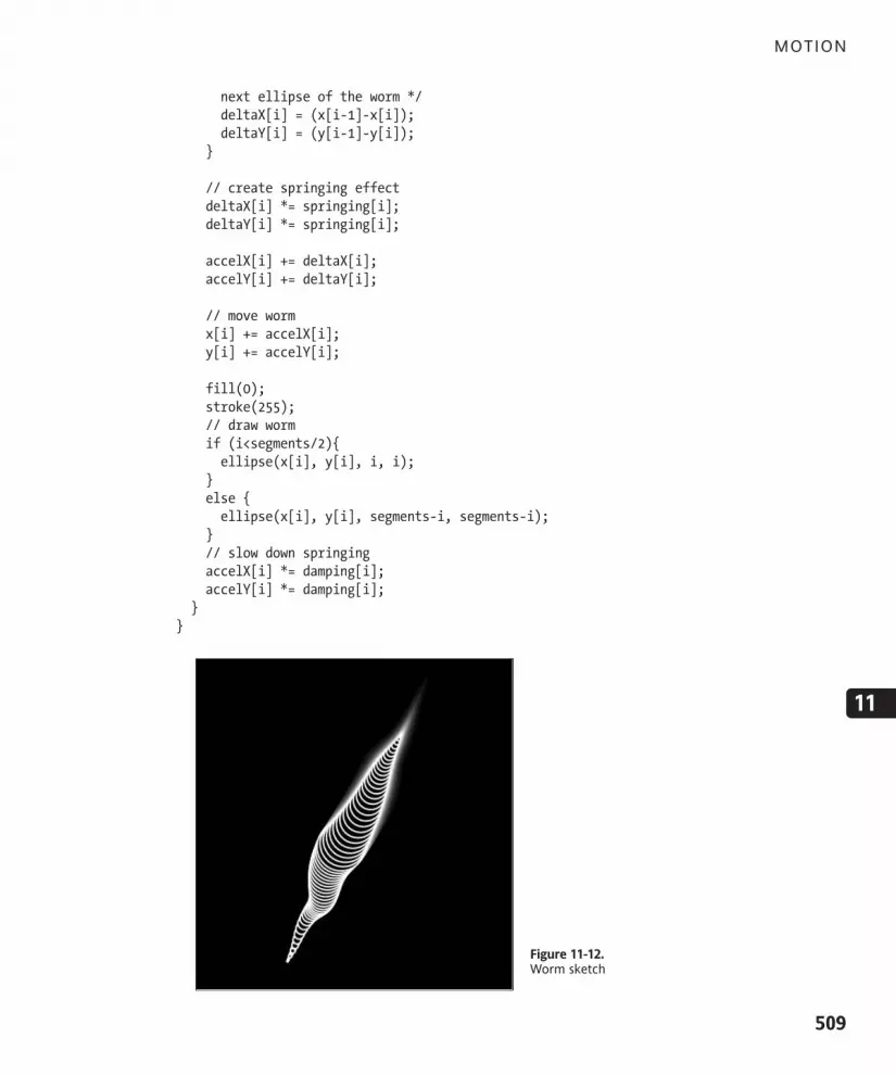
next ellipse of the worm */deltaX[i] = (x[i-1]-x[i]);deltaY[i] = (y[i-1]-y[i]);
}
// create springing effectdeltaX[i] *= springing[i];deltaY[i] *= springing[i];
accelX[i] += deltaX[i];accelY[i] += deltaY[i];
// move wormx[i] += accelX[i];y[i] += accelY[i];
fill(0);stroke(255);// draw wormif (i<segments/2){ellipse(x[i], y[i], i, i);
}else {ellipse(x[i], y[i], segments-i, segments-i);
}// slow down springingaccelX[i] *= damping[i];accelY[i] *= damping[i];
}}
Figure 11-12.Worm sketch
MOTION
509
11
617xCH11.qxd 4/17/07 1:57 PM Page 509

Earlier in the chapter, when we converted a single bouncing rectangle to multiple bounc-ing rectangles, the problem mostly boiled down to converting single variables to arraysand using for loops in setup() and draw() to process them; this is pretty much the casewith this last example. The springing principle works similarly to the previous RavenousTriangle II example. There are, however, two aspects that probably need clarification.
The first challenge with the worm was keeping the springing values within a logical rangeso that the worm moved properly (based on my own aesthetic sense). I actually have noidea about real worm motility—other than I suspect it involves slithering.
First, notice the for loop:
for (int i=0; i<segments; i++){/* need to decrease both springing and damping values as segments increase */springing[i] = .05*(.07*(i+1));damping[i] = .95-(.02*i);
}
This is where I initialized the springing[] and damping[] array values. I settled on the twoscary-looking expressions after some trial and error. I suspect other values could yieldeven nicer worm movement. Since the springing of the ellipses, other than the initial one,are based on each preceding ellipse, the springing values increased rapidly, creating aninteresting expanding and whipping wave pattern, but not a solid slithering worm. Byreducing the values of both the springing and damping each iteration of the for loop, Iwas able to find a workable worm solution. Again, I urge you to mess around with thesevalues, obliterating the worm in the process—it won’t feel a thing.
For the food source, I wanted to created a simple wandering (invisible) bot that wouldreplace mouseX and mouseY in calculating the deltaX and deltaY values. I needed the foodsource (fx, fy) to only control the lead ellipse, and I needed the other ellipses to each becontrolled by the preceding ellipse. Here’s the block of code that handles this:
// lead ellipseif (i==0){/* food position used to calculate theinitial ellipse of the worm */deltaX[i] = (fx-x[i]);deltaY[i] = (fy-y[i]);
}else {/* preceding ellipse used to calculate the
next ellipse of the worm */deltaX[i] = (x[i-1]-x[i]);deltaY[i] = (y[i-1]-y[i]);
}
The food source itself wanders around the display window based on trig functions withsome random values. It also bounces off the display window boundaries, keeping theworm on the screen.
PROCESSING: CREATIVE CODING AND COMPUTATIONAL ART
510
617xCH11.qxd 4/17/07 1:57 PM Page 510

Finally, the following code, which draws the actual worm, might need a little explanation:
stroke(255);// draw wormif (i<segments/2){ellipse(x[i], y[i], i, i);
}else {ellipse(x[i], y[i], segments-i, segments-i);
}
I wanted the worm to have both a narrow anterior and posterior and a wider midsection.The if...else block ensures that the ellipses would form in this basic structure. Again, trymessing with these values to create some other strange organisms.
An alternative spring approachThere is another way of simulating springs that some people may find easier than theapproach we just looked at. Consider the motion of a spring—does it suggest any otherform? A spring undulates, usually symmetrically, in a regular wave pattern. Thus, any equa-tion that generates a wave should be able to simulate wave behavior. We used the trigfunctions in Chapter 7 (on curves) to create waves, and we can use them here as well tosimulate spring behavior.
The next example, shown in Figure 11-13, is of a fairly realistic weight on a spring thatstretches as the weight moves. Clicking the screen resets the spring.
// Weight on a Springfloat x, y;int w = 150, h = 100;float angle, frequency = 5.0;float amplitude, damping = .987;int springSegments = 32, springWidth = 15;
void setup(){size(400, 400);x = width/2.0-w/2.0;smooth();strokeWeight(5);fill(0);setSpring();
}
void draw(){background(255);createSpring();startSpring();
}
MOTION
511
11
617xCH11.qxd 4/17/07 1:57 PM Page 511

void startSpring(){// spring behaviory += cos(radians(angle))*amplitude;amplitude*=damping;angle+=frequency;
if (mousePressed){setSpring();
}}
void setSpring(){y = 100;angle = 0;amplitude = 26.0;
}
void createSpring(){// weightquad(x+20, y, x+w-20, y, x+w, y+h, x, y+h);// springfor (int i=0; i<springSegments; i++){// end segmentif (i==springSegments-1){line(x+w/2+springWidth, (y/springSegments)*i, !
x+w/2, (y/springSegments)*(i+1));}else {// alternate spring bend left/rightif (i%2==0){line(x+w/2-springWidth, (y/springSegments)*i, !
x+w/2+springWidth, (y/springSegments)*(i+1));}else {line(x+w/2+springWidth, (y/springSegments)*i, !
x+w/2-springWidth, (y/springSegments)*(i+1));}
}}
}
PROCESSING: CREATIVE CODING AND COMPUTATIONAL ART
512
617xCH11.qxd 4/17/07 1:57 PM Page 512

Figure 11-13. Weight on a Spring sketch
Notice the actual springing code in the setSpring() function:
// spring behaviory += cos(radians(angle))*amplitude;amplitude*=damping;angle+=frequency;
This code is very similar to other trig expressions used throughout the book. Again, bydamping a simple sine or cosine wave over time, you can create pretty realistic springmotion. Lastly, notice within the createSpring() function that I used the modulus opera-tor (%) when drawing the spring. I needed a way of alternating the plotting of the springcoil right and left. By using the if...else block with the condition (i%2==0)—only aneven number leaves a remainder of 0 when divided by 2—I was able to accomplish thiseasily.
We can build upon this concept by simulating some values for mass and spring strength. Inthe next sketch, shown in Figure 11-14, I create a series of springs that have varying sizes(representing differences in mass) and spring strengths, illustrated by varying the strokeweight when drawing the springs. Based on these variations, the sketch simulates howthese different configurations might move. For example, a heavy weight attached to aspring with a small rod diameter would stretch further than the same weight on a springwith a wider diameter. The damping effect of the spring is based on the stroke weight aswell. Each time you run the sketch or click the mouse in the display window, randomvalues are generated for mass and spring strengths.
// Weights on Springsint weights = 5;float[]x = new float[weights];float[]y = new float[weights];float[]w = new float[weights];float[]h = new float[weights];float[]angle = new float[weights];
MOTION
513
11
617xCH11.qxd 4/17/07 1:57 PM Page 513

float[]frequency = new float[weights];float[]amplitude = new float[weights];float[]strokeWt = new float[weights];float[]damping = new float[weights];int springSegments = 24, springWidth = 8;
void setup(){size(600, 400);frameRate(30);smooth();fill(0);setSpring();
}
void draw(){background(255);for (int i=0; i<weights; i++){createSpring(x[i], y[i], w[i], h[i], strokeWt[i]);noStroke();fill(0);// draw weightsquad(x[i], y[i], x[i]+w[i], y[i], x[i]+w[i]+w[i]*.2, !
y[i]+h[i], x[i]-w[i]*.2, y[i]+h[i]);// spring behaviory[i] = y[i]+cos(radians(angle[i]))*amplitude[i];angle[i]+=frequency[i];amplitude[i]*=damping[i];
}// press the mouse to resetif (mousePressed){setSpring();
}}
void setSpring(){for (int i=0; i<weights; i++){// size approximates massw[i] = random(20, 70);h[i] = w[i];// stroke weight approximates // spring strength (resistance)strokeWt[i] = random(1, 4);x[i] = ((width/(weights+1))*i)+width/(weights+1)-w[i]/2.0;y[i] = (w[i]*3)/strokeWt[i];angle[i] = 0;// spring speedfrequency[i] = strokeWt[i]*4;// amplitude based on mass/spring strengthamplitude[i] = (w[i]*1.5)/strokeWt[i];
PROCESSING: CREATIVE CODING AND COMPUTATIONAL ART
514
617xCH11.qxd 4/17/07 1:57 PM Page 514

// calc. damping based on strokeWeight// simulates resistance of spring thicknessswitch(round(strokeWt[i])){case 1:damping[i] = .99;break;
case 2:damping[i] = .98;break;
case 3:damping[i] = .97;break;
case 4:damping[i] = .96;break;
}}
}
//plot springvoid createSpring(float x, float y, float w, float h, float strokeWt){stroke(50);strokeWeight(strokeWt);for (int i=0; i<springSegments; i++){// for spring end segmentif (i==springSegments-1){line(x+w/2+springWidth, (y/springSegments)*i, !
x+w/2, (y/springSegments)*(i+1));}else {// alternate spring bend left/rightif (i%2==0){line(x+w/2-springWidth, (y/springSegments)*i, !
x+w/2+springWidth, (y/springSegments)*(i+1));}else {line(x+w/2+springWidth, (y/springSegments)*i, !
x+w/2-springWidth, (y/springSegments)*(i+1));}
}}
}
MOTION
515
11
617xCH11.qxd 4/17/07 1:57 PM Page 515

Figure 11-14. Weights on Springs sketch
Even the simplest wavy/springy behavior can be evocative and even humorous. I’ve cre-ated two final spring examples that illustrate this. The first sketch is of a simple undulatingsine wave that moves across the display window. When I showed the initial state of thissketch to my six-year-old son, he immediately saw its connection to the way water moves,so I added an additional playful element. This example, entitled Beach Ball, is a bit long, soI’ve provided it as a download, which you can find in the Download section of the friendsof ED website (www.friendsofed.com/downloads.html).
Soft-body dynamicsThe second example is of a springy polygon that combines both approaches to springingwe’ve looked at this chapter. This sketch is loosely inspired by the brilliant Java workSodaplay (www.sodaplay.com/constructor/index.htm), created by Ed Burton and team atSoda Creative (http://soda.co.uk/). The example illustrates (very) simple soft-bodydynamics. In rigid-body dynamics, objects collide and interact, but the objects themselvesdon’t deform; think of a block of wood falling down the stairs. In soft-body dynamics, theobjects actually deform; think of a water balloon falling down the stairs (but not explod-ing). People are often fascinated by these types of simulations (I know I am), and in manyways they represent the ultimate illusion. Since we are more or less squishy, soft-bodiedorganisms ourselves, these types of soft-body physics simulations represent a logicalextension of earlier creative attempts at human depiction—from cave paintings, to terracotta figures, to self-portraiture, to Shrek’s bouncing belly. Following is the code forHybrid Springy Dude: A Polygon with Attitude (shown in Figure 11-15):
/* Hybrid Springy Dude:A Polygon with Attitude */// center pointfloat centerX = 0, centerY = 0;float radius = 60, rotAngle = -90;float accelX, accelY;float springing = .0085, damping = .98;
PROCESSING: CREATIVE CODING AND COMPUTATIONAL ART
516
617xCH11.qxd 4/17/07 1:57 PM Page 516

//corner nodesint nodes = 5;float nodeStartX[] = new float[nodes];float nodeStartY[] = new float[nodes];float[]nodeX = new float[nodes];float[]nodeY = new float[nodes];float[]angle = new float[nodes];float[]frequency = new float[nodes];// soft-body dynamicsfloat organicConstant = 1;
void setup(){size(400, 400);//center shape in windowcenterX = width/2;centerY = height/2;// initialize frequencies for corner nodesfor (int i=0; i<nodes; i++){frequency[i] = random(5, 12);
}noStroke();frameRate(30);
}
void draw(){//fade backgroundfill(255, 100);rect(0,0,width, height);drawShape();moveShape();
}
void drawShape(){// calculate node starting locationsfor (int i=0; i<nodes; i++){nodeStartX[i] = centerX+cos(radians(rotAngle))*radius;nodeStartY[i] = centerY+sin(radians(rotAngle))*radius;rotAngle += 360.0/nodes;
}
// draw polygoncurveTightness(organicConstant);fill(175);beginShape();for (int i=0; i<nodes; i++){curveVertex(nodeX[i], nodeY[i]);
}for (int i=0; i<nodes-1; i++){curveVertex(nodeX[i], nodeY[i]);
MOTION
517
11
617xCH11.qxd 4/17/07 1:57 PM Page 517

}endShape();
}
void moveShape(){//move center pointfloat deltaX = mouseX-centerX;float deltaY = mouseY-centerY;
// create springing effectdeltaX *= springing;deltaY *= springing;accelX += deltaX;accelY += deltaY;
// move polygon's centercenterX += accelX;centerY += accelY;
// slow down springingaccelX *= damping;accelY *= damping;
// change curve tightnessorganicConstant = 1-((abs(accelX)+abs(accelY))*.1);
//move nodesfor (int i=0; i<nodes; i++){nodeX[i] = nodeStartX[i]+sin(radians(angle[i]))*(accelX*2);nodeY[i] = nodeStartY[i]+sin(radians(angle[i]))*(accelY*2);angle[i]+=frequency[i];
}}
Figure 11-15. Hybrid Springy Dude sketch
PROCESSING: CREATIVE CODING AND COMPUTATIONAL ART
518
617xCH11.qxd 4/17/07 1:57 PM Page 518

Springy Dude is not an accurate physics simulation. Instead, I used some random values asan approximation for the spring and deformation. When the mouse moves, the entirepolygon springs, based on the original springing code we looked at earlier in the chapter.The block of code controlling this overall movement is the following:
// move center pointfloat deltaX = mouseX-centerX;float deltaY = mouseY-centerY;
// create springing effectdeltaX *= springing;deltaY *= springing;accelX += deltaX;accelY += deltaY;
// move polygon's centercenterX += accelX;centerY += accelY;
// slow down springingaccelX *= damping;accelY *= damping;
I utilized a parenting approach with regard to the relationship between the polygon’s fiveperimeter points (which aren’t rendered) and the shape’s central point. If you haven’tdone much computer animation before, this may not initially mean much to you. The cen-tral problem in a sketch like Hybrid Springy Dude is how to maintain the shape, whileallowing both the form to move as a whole and its individual parts to move independently.
In a program like Flash, there are MovieClip data structures that can explicitly have parentand nested child clips. Most 3D animation applications employ similar constructs. InProcessing, we don’t have this built-in structure (though of course we could build one).Instead, in the example I used the variables centerX and centerY to represent the overallcoordinating point of the entire shape, which in a sense becomes the parent (or controlnode).
I used trig functions both to calculate the nodes’ starting positions (relative to the shape’scenter point) and to create the spring effect on the shape’s vertices. To enable the shapeto return to its original polygonal structure after the springing, I needed to capture theoriginal point locations of the shape (relative to the control node). Here’s the block ofcode that does that:
// calculate node starting locationsfor (int i=0; i<nodes; i++){nodeStartX[i] = centerX+cos(radians(rotAngle))*radius;nodeStartY[i] = centerY+sin(radians(rotAngle))*radius;rotAngle += 360.0/nodes;
}
MOTION
519
11
617xCH11.qxd 4/17/07 1:57 PM Page 519

The nodes are then moved with two other trig expressions:
//move nodesfor (int i=0; i<nodes; i++){nodeX[i] = nodeStartX[i]+sin(radians(angle[i]))*(accelX*2);nodeY[i] = nodeStartY[i]+sin(radians(angle[i]))*(accelY*2);angle[i]+=frequency[i];
}
The two blocks of code are very similar. Again, the first block captures the nodes’ originalpositions, which keep changing as the overall shape is moving. The second code blocktakes care of moving the individual points. The springing movement of both the overallform and the individual points is controlled by the variables accelX and accelY, which arecalculated in the overall spring code shown earlier.
Finally, the curvy deformation—from a rigid polygonal structure to an organic blob—isbased on the following line:
// change curve tightnessorganicConstant = 1-((abs(accelX)+abs(accelY))*.1);
This line calculates a curve tightness value, which is fed into Processing’s curveTightness()function when the shape is plotted, using a series of curveVertex() calls:
// draw polygoncurveTightness(organicConstant);fill(175);beginShape();for (int i=0; i<nodes; i++){curveVertex(nodeX[i], nodeY[i]);
}for (int i=0; i<nodes-1; i++){curveVertex(nodeX[i], nodeY[i]);
}endShape();
You may remember from Chapter 7 (“Curves”) that the curveTightness() function con-trols how the curve interpolation is handled between the curve vertices. I took advantageof this really handy and simple-to-use function to create all the squishy, soft-body magic.
Advanced motion and object collisionsEarlier in the chapter we looked at a simple strategy for handling the collision of objectswith the display window. The steps included placing the object flush with the edge in casethe detection happened after the object had already passed through the edge, and thenreversing the speed value controlling the object’s motion—this was done for both axes.Here’s another simple example of this basic collision approach:
PROCESSING: CREATIVE CODING AND COMPUTATIONAL ART
520
617xCH11.qxd 4/17/07 1:57 PM Page 520

float x, y, r = 20;float speedX = 2, speedY = 2.5;void setup(){size(400, 400);x = width/2;y = height/2;noStroke();smooth();
}void draw(){background(0);x+=speedX;y+=speedY;ellipse(x, y, r*2, r*2);// check wall collisionsif (x > width-r){x = width-r;speedX*=-1;
}else if (x < r){x = r;speedX*=-1;
}else if (y > height-r){y = height-r;speedY*=-1;
}else if (y < r){y = r;speedY *=-1;
}}
This strategy will work fine for orthogonal collisions, when the object bounces off a hori-zontal or vertical surface. However, it won’t work for an object hitting an angular or curvedsurface, including objects colliding with each other. The next section will show you how todeal with these cases.
VectorsTo begin to think about these more advanced types of collisions, you need to considerhow an object’s path is controlled by the speed values you increment it by. In the lastexample, I incremented x by 2 and y by 2.5. Obviously, since y is being increased moreeach frame than is x, the object moves on more of a vertical path than a horizontal one.Since neither speed value was 0, you could also predict that the object would move insome type of diagonal path. If speedX had been 0, the object would have only moved ver-tically. And of course the situation would have been reversed if speedY had been 0.
MOTION
521
11
617xCH11.qxd 4/17/07 1:57 PM Page 521
Returning to the original speed settings, speedX = 2, speedY = 2.5, what could you do ifyou wanted to double the speed of the object, but not alter its direction? You could mul-tiply both values by 2. This would cause the object to move faster, but still along the samepath. So what happened? I know this may seem pathetically simple, but the underlyingconcepts are very important for what we’ll be doing (and not as simple as they may initiallyseem).
When you double the speed settings, the object’s speed obviously increases, but the ratioof the two speeds remains the same, keeping the object moving in the same direction. Thisratio relates to the slope of the line defining the movement of the object. You may recallthat slope is calculated as the change in y (!y) over the change in x (!x)—or the rise overthe run.
Thus, speed and direction can be thought of as two separate quantities; you can alter anobject’s speed while still maintaining its current direction. (It would be pretty hard to drivea car safely if we couldn’t do this.) Mathematically, there is a convenient way of expressingall this, namely in a structure called a vector.
I’ve mentioned vectors earlier in the book, and we’ll delve deeper into them in the finalchapters (on 3D) as well. A vector, for our current purposes, is a quantity that describesboth speed and direction, more commonly known as velocity.
In the next example, the two parts of the vector (direction and speed) are coded as sepa-rate variables, to help illustrate their relationship. The sketch moves five rectangles in thesame direction, but at differing speeds.
float directionX = .56, directionY = .83;float[] speeds = {.75, 1.3, 2.2, .92, 1.5};float[] x = new float[5], y = new float[5];
void setup(){size(400, 400);noStroke();fill(128);smooth();
}void draw(){background(255);for (int i=0; i<5; i++){x[i] += directionX*speeds[i];y[i] += directionY*speeds[i];rect(x[i], y[i], 6, 6);
}}
The variables directionX and directionY represent the direction the rectangles all travel.The specific values .56 and .83 can be thought of as the base ratio of change along x andy, respectively. In other words, even if we multiply both of these values by some very largecommon constant, we increase the overall speed value, but we don’t affect the ratiobetween these two values (which again controls the direction the rectangles are moving).
PROCESSING: CREATIVE CODING AND COMPUTATIONAL ART
522
617xCH11.qxd 4/17/07 1:57 PM Page 522

Normalizing a vectorWhen working with vectors, it is common practice to find this base ratio of a vector, whichis referred to as normalizing a vector. Normalizing simply means reducing the magnitude(length) of a vector to 1, which is done by dividing each component of a vector by its over-all length. For example if you have vector v, you can find its length like this (expressed incode):
length = sqrt(v.x*v.x + v.y*v.y);
Then to find the base ratio, you simply divide each of the vector’s components by itslength:
normalizedVector.x = v.x / length;normalizedVector.y = v.y / length;
Again, this base ratio, or normalized vector, expresses the direction of the vector. Forexample, if we have a line and we want to animate an ellipse at a certain speed along theline, we can treat the line as a vector. Once we have the length of the line, we can nor-malize it and use the normalized values as the direction for the ellipse to travel, which wecan then multiply by any speed we choose. Here’s a sketch that does precisely this (shownin Figure 11-16):
// Moving Along a Vectorfloat lineX1, lineY1, lineX2, lineY2;float vectX, vectY, vectMag, directionX, directionY;float ellipseX, ellipseY;float ellipseSpeed = 2;
void setup(){size(400, 400);fill(128);smooth();lineX1 = 100;lineY1 = 75;lineX2 = 300;lineY2 = 325;
// express line as a vectorvectX = lineX2-lineX1;vectY = lineY2-lineY1;
// find magnitude(length) of vectorvectMag = sqrt(vectX*vectX + vectY*vectY);
/* normalize vector to get base direction ratio */directionX = vectX/vectMag;directionY = vectY/vectMag;
MOTION
523
11
617xCH11.qxd 4/17/07 1:57 PM Page 523

// start ellipse on lineellipseX = lineX1;ellipseY = lineY1;
}void draw(){background(255);// draw lineline(lineX1, lineY1, lineX2, lineY2);
//draw ellipseellipse(ellipseX, ellipseY, 20, 20);
// move elipseellipseX += directionX * ellipseSpeed;ellipseY += directionY * ellipseSpeed;
// keeps ellipse moving along lineif (ellipseX>lineX2 && ellipseY>lineY2 ||ellipseX<lineX1 && ellipseY<lineY1) {/* when ellipse reaches end of vectorreverse the vector's direction */directionX *= -1;directionY *= -1;
}}
Figure 11-16. Moving Along a Vector sketch
In the sketch, I calculated the line as a vector by finding the difference between the com-ponents (x and y) of each endpoint of the line (x2 – x1, y2 – y1). Since I subtracted the left-most point of the line from the right, I found component values independent of the
PROCESSING: CREATIVE CODING AND COMPUTATIONAL ART
524
617xCH11.qxd 4/17/07 1:57 PM Page 524

placement of the vector within the larger coordinate system. This is actually a feature ofvectors; it doesn’t matter where you put them—their direction and magnitude will remainconstant.
Once I got the vector’s components, I simply calculated the vector’s overall length andthen divided each component by this length, giving me the base direction ratio, which Iused in the calculation to move the ellipse, independent of the ellipse’s speed.
Applying vectors in collisionsLet’s now apply some of these vector principles to collisions. You already know how tohandle collisions against orthogonal surfaces, such as the display window boundaries.However, the problem is quite a bit more complex when the collision surface is not orthog-onal. The reason for this added complexity essentially boils down to a rotated coordinatesystem problem. For example, in Figure 11-17, the collision depicted on the left takes placeagainst an orthogonal surface. The collision on the right, against a non-orthogonal surface,can also be thought of as an orthogonal collision in a rotated coordinate system. As youmight guess, one solution to solving a non-orthogonal collision problem is to factor in thiscoordinate rotation. I’ll discuss this solution shortly. First, however, I want to look atanother approach, borrowing a principle from physics: the law of reflection.
Figure 11-17. Orthogonal vs. non-orthonal collisions
The law of reflectionFigure 11-18 illustrates the law of reflection, which simply states that when light strikes asurface, the angle of reflection is equal to the angle of incidence, relative to the surfacenormal. The angle of incidence is the angle of the incoming ray striking the surface. A nor-mal line is any line perpendicular to a surface. (It actually doesn’t matter where on the sur-face this line is, since all perpendicular lines off a flat surface will be parallel.) Please alsonote that the terms surface normal and normalizing a vector are unrelated. Rememberthat normalizing involves dividing a vector’s components by the length of the vector. Infact, in the next example, I’ll actually be normalizing the surface normal. Although this lawof reflection relates to how light reflects off of a surface, it works the same way for anobject bouncing off a surface.
MOTION
525
11
617xCH11.qxd 4/17/07 1:57 PM Page 525

Figure 11-18. Law of reflection
There is a very handy equation you can use to apply this principle: R = 2N(N • L) – L, whereR is the reflection vector, N is the surface normal (also a vector quantity), and L is the inci-dent vector. Both the normal vector and the incident vector need to be normalized as well.The expression (N • L) represents the dot product of the surface normal and the incidentvector. Since N and L are both vector quantities, you can’t simply multiply them togetherthe way you do two individual values (e.g., 5 " 4). Instead, you have two options for mul-tiplying vectors; one approach returns a single non-vector value (the dot product) and theother approach returns another vector (the cross-product). For this example, you onlyneed to use the dot product calculation. When you get to Chapter 14, you’ll use the cross-product along with the dot product.
The beauty of using this equation is that you don’t have to worry about rotating coordi-nates. In the next example (shown in Figure 11-19), I created a non-orthogonal base planefor the ellipse to deflect off of. To handle the actual collision detection, I treated the topof the base as an array of point coordinates and checked the distance between the ellipseand each of the individual points. Each time the ellipse hits the top of the display window,the base top is recalculated.
/********************************************** Non-orthogonal Reflection:* Based on the equation R = 2N(N•L)-L * R = reflection vector* N = normal* L = incidence vector
PROCESSING: CREATIVE CODING AND COMPUTATIONAL ART
526
617xCH11.qxd 4/17/07 1:57 PM Page 526

Ira Greenberg, 2/12/07********************************************/float baseX1, baseY1, baseX2, baseY2;float baseLength;float[] xCoords, yCoords;float ellipseX, ellipseY, ellipseRadius = 8;float directionX, directionY;float ellipseSpeed = 3.5;float velocityX, velocityY;
void setup(){size(400, 400);fill(128);smooth();baseX1 = 0;baseY1 = height-150;baseX2 = width;baseY2 = height;
// start ellipse at middle top of screenellipseX = width/2;
// calculate initial random directiondirectionX = random(.1, .99);directionY = random(.1, .99);
// normalize direction vectorfloat directionVectLength = sqrt(directionX*directionX + !
directionY*directionY);directionX /= directionVectLength;directionY /= directionVectLength;
}
void draw(){// draw backgroundfill(0, 6);noStroke();rect(0, 0, width, height);
// calculate length of base topbaseLength = dist(baseX1, baseY1, baseX2, baseY2);xCoords = new float[ceil(baseLength)];yCoords = new float[ceil(baseLength)];
// fill base top coordinate arrayfor (int i=0; i<xCoords.length; i++){xCoords[i] = baseX1 + ((baseX2-baseX1)/baseLength)*i;yCoords[i] = baseY1 + ((baseY2-baseY1)/baseLength)*i;
}
MOTION
527
11
617xCH11.qxd 4/17/07 1:57 PM Page 527

// draw basefill(200);quad(baseX1, baseY1, baseX2, baseY2, baseX2, height, 0, height);
// calculate base top normalfloat baseDeltaX = (baseX2-baseX1)/baseLength;float baseDeltaY = (baseY2-baseY1)/baseLength;float normalX = -baseDeltaY;float normalY = baseDeltaX;
// draw ellipsenoFill();stroke(200);ellipse(ellipseX, ellipseY, ellipseRadius*2, ellipseRadius*2);
// calculate ellipse velocityvelocityX = directionX * ellipseSpeed;velocityY = directionY * ellipseSpeed;
// move elipseellipseX += velocityX;ellipseY += velocityY;
// normalized incidence vectorfloat incidenceVectorX = -directionX;float incidenceVectorY = -directionY;
// detect and handle collisionfor (int i=0; i<xCoords.length; i++){// check distance between ellipse and base top coordinatesif (dist(ellipseX, ellipseY, xCoords[i], !
yCoords[i]) < ellipseRadius){
// calculate dot product of incident vector and base top normalfloat dot = incidenceVectorX*normalX + !
incidenceVectorY*normalY;
// calculate reflection vectorfloat reflectionVectorX = 2*normalX*dot - incidenceVectorX;float reflectionVectorY = 2*normalY*dot - incidenceVectorY;
// assign reflection vector to direction vectordirectionX = reflectionVectorX;directionY = reflectionVectorY;
// draw base top normal at collision pointstroke(255, 128, 0);line(ellipseX, ellipseY, ellipseX-normalX*100, !
ellipseY-normalY*100);
PROCESSING: CREATIVE CODING AND COMPUTATIONAL ART
528
617xCH11.qxd 4/17/07 1:57 PM Page 528

}}
// detect boundary collision// rightif (ellipseX > width-ellipseRadius){ellipseX = width-ellipseRadius;directionX *= -1;
}// leftif (ellipseX < ellipseRadius){ellipseX = ellipseRadius;directionX *= -1;
}// topif (ellipseY < ellipseRadius){ellipseY = ellipseRadius;directionY *= -1;// randomize base topbaseY1 = random(height-300, height);baseY2 = random(height-300, height);
}}
Figure 11-19. Non-orthogonal Reflection sketch
MOTION
529
11
617xCH11.qxd 4/17/07 1:57 PM Page 529

This is not a simple example, so I expect some of you may be scratching your heads a bitreviewing the code. Notice at the top of the sketch, where I declared global variables, thatI created separate variables for directionX, directionY, and ellipseSpeed. Similarly, as inthe last example, I conceptualized the ellipse’s movement as a vector quantity, keepingdirection and speed as separate quantities. I also declared initial arbitrary values fordirectionX and directionY. These two variables represent the direction of the incident(incoming) vector. This vector must be normalized to be useful in the larger reflection cal-culation (R = 2N(N • L) – L). I normalized the vector at the bottom of the setup() func-tion, with the following lines:
// normalize direction vectorfloat directionVectLength = sqrt(directionX*directionX + !
directionY*directionY);directionX /= directionVectLength;directionY /= directionVectLength;
You’ll remember that to normalize a vector, you need to divide each of the vector’s com-ponents by the overall length of the vector, which I did in the previous code snippet. Sincethe variables directionX and directionY are randomly assigned values, I couldn’t assumethat they formed a vector with a length of 1 (the length of a normalized vector).
Within the draw() function, I used the following lines to calculate the coordinate values ofthe top of the base, which were used in the collision detection:
// calculate length of base topbaseLength = dist(baseX1, baseY1, baseX2, baseY2);xCoords = new float[ceil(baseLength)];yCoords = new float[ceil(baseLength)];
// fill base top coordinate arrayfor (int i=0; i<xCoords.length; i++){xCoords[i] = baseX1 + ((baseX2-baseX1)/baseLength)*i;yCoords[i] = baseY1 + ((baseY2-baseY1)/baseLength)*i;
}
I used the length of the base top edge to instantiate two float arrays of the same length.Since the baseLength calculation resulted in a float value, I was forced to convert thefloat value to an int value to be able to use this value to initialize the lengths of the twoarrays. Next, using the for loop, I filled the two arrays with the coordinate values formingthe base top edge. I’ll assume you can make sense of the code that draws and moves theellipse, as we’ve looked at code like this before, including in the last example.
To calculate the base top edge’s normal, I needed to first generate the vector forming thetop edge of the base. I also normalized this vector. Both of these steps were taken care ofin the first two lines (following the comment) of the following code:
// calculate base top normalfloat baseDeltaX = (baseX2-baseX1)/baseLength;float baseDeltaY = (baseY2-baseY1)/baseLength;float normalX = -baseDeltaY;float normalY = baseDeltaX;
PROCESSING: CREATIVE CODING AND COMPUTATIONAL ART
530
617xCH11.qxd 4/17/07 1:57 PM Page 530

In two dimensions, the surface normal of a vector is really just a line perpendicular to thevector. In three dimensions, the situation is a bit more complicated and requires the use ofthe cross-product calculation mentioned previously. We’ll look at the cross-product in thebook’s final chapter. Calculating the perpendicular line to a vector is very simple. To getthe x component of the normal, you simply reverse the sign of the vector’s y component,and to get the y component of the normal, you take the vector’s x component, as illus-trated in the last two lines of the previous snippet of code. Be aware, though, that everyvector actually has two perpendicular lines, facing opposite directions (once you knowone, just reverse its sign to find the other).
The block of code that handles most of the real heavy lifting in the draw() function is thefollowing:
// normalized incidence vectorfloat incidenceVectorX = -directionX;float incidenceVectorY = -directionY;
// detect and handle collisionfor (int i=0; i<xCoords.length; i++){// check distance between ellipse and base top coordinatesif (dist(ellipseX, ellipseY, xCoords[i], !
yCoords[i]) < ellipseRadius){
// calculate dot product of incident vector and base top normalfloat dot = incidenceVectorX*normalX + !
incidenceVectorY*normalY;
// calculate reflection vectorfloat reflectionVectorX = 2*normalX*dot - incidenceVectorX;float reflectionVectorY = 2*normalY*dot - incidenceVectorY;
// assign reflection vector to direction vectordirectionX = reflectionVectorX;directionY = reflectionVectorY;
// draw base top normal at collision pointstroke(255, 128, 0);line(ellipseX, ellipseY, ellipseX-normalX*100, !
ellipseY-normalY*100);}
}
The directionX and directionY variables were normalized earlier in the sketch, so all Ineeded to do was reverse their signs to generate the normalized incidence vector(incidenceVectorX and incidenceVectorY). The for loop iterates though all the coordi-nates forming the base’s top edge, and the conditional statement checks if the ellipse’sdistance relative to the base’s top edge is less than the ellipse’s radius—in which case acollision is detected. Once detected, the dot product is calculated by multiplying the inci-dence vector and normal vector’s x and then y components, respectively, and adding thesevalues together. This calculation works the same way for three dimensions—by simply
MOTION
531
11
617xCH11.qxd 4/17/07 1:57 PM Page 531

adding the z component into the mix. I’m not going to go into the theory behind the dotproduct here, but I will discuss it when I cover 3D in Chapter 14. If you just can’t wait,though, Wikipedia has some good stuff to say about it at http://en.wikipedia.org/wiki/Dot_product.
Following the dot product calculation, I calculate the reflection vector, plugging in the val-ues I’ve previously calculated. Finally, I assign the reflection vector to the original directionvector and display the normal at the point of collision. If the code is working, you shouldsee that the angle formed between the base edge normal and the incoming incidence vec-tor is equal to the angle between the outgoing reflection vector and the normal. Theremainder of the code handles display window boundary detection and also resets thebase’s top edge whenever the ellipse makes contact with the top of the display window.
A better way to handle non-orthogonal collisionsAlthough the last example successfully handled angled collisions, there are some chal-lenges in trying to extend this solution to handle object-object collisions as well trying toadd simple physics, like gravity and drag. There is another collision solution thatActionScript guru Keith Peters writes about in his excellent book Foundation ActionScriptAnimation: Making Things Move! Although Keith’s book deals with ActionScript, notProcessing, I highly recommend it as a general graphics coding guide.
The solution Keith writes about deals with considering angled collisions as a rotated coor-dinate system problem, instead of focusing on trying to calculate the actual reflectionangle. It works like this: if you take any 2D collision, you can always rotate the local coor-dinates so that the collision happens orthogonally (shown in Figure 11-20). For example,suppose a ball strikes a surface at a 40-degree angle. Rather than trying to calculate theangle of reflection, taking into account both the ball’s incidence vector and the angle ofthe collision surface, you can rotate the surface and velocity vector (in this case –40degrees) so that the collision surface is orthogonal (perfectly horizontal or vertical). Oncerotated, you can handle the reflection the same way you do with collisions against theedges of the display window—simply reverse the sign of the appropriate velocity vectorcoordinate; finally, the last step is rotating everything back to where it was prior to therotation.
Figure 11-20. Handling non-orthogonal collisions by rotating coordinates
PROCESSING: CREATIVE CODING AND COMPUTATIONAL ART
532
617xCH11.qxd 4/17/07 1:57 PM Page 532

We’ll look at this process in steps. The first step is handling the rotation of the collisionsurface and velocity vector. Remember your trusted rotation expressions:
x = cos(theta)*radiusy = sin(theta)*radius
These expressions hopefully look very familiar by now. They allow you to plot any pointbased on theta (the angle of rotation expressed in radians) and a radius. These equationsare immensely handy in code art. However, there is another somewhat more complicatedform of the expressions that makes them even handier (and absolutely essential for calcu-lating 3D rotations). The two expressions just mentioned are actually derived from theirmore powerful trig brethren:
new x = cos(theta)*x - sin(theta)*ynew y = cos(theta)*y + sin(theta)*x
Whoa! Now don’t freak out yet. The main difference between the two forms of the expres-sions is that the familiar shorter ones are used when the angle of rotation begins at 0. Thelonger forms of the expressions are used when the rotation represents a change of rota-tion (not necessarily beginning at 0 on the unit circle) and is also based on a specific pointlocation (x and y). In the next example, I’ll use these expressions to rotate a simple linearound the center point of the display window (press the mouse to make the line rotatefrom its current position):
/* Trig Rotation Expressions-mouse press to rotateSpecial thanks to kirupa.com*/
float[] x = new float[2];float[] y = new float[2];float[] newX = new float[2];float[] newY = new float[2];float theta;
void setup(){size(400, 400);float t = random(TWO_PI);/* I used the simple trig rotation form to generate the original line coords */x[0] = cos(t)*-50;y[0] = sin(t)*-50;x[1] = cos(t)*50;y[1] = sin(t)*50;
}
void draw(){background(255);translate(width/2, height/2);/* I used the longer trig rotation form to rotate based on the existing rotation */
MOTION
533
11
617xCH11.qxd 4/17/07 1:57 PM Page 533

newX[0] = cos(theta)*x[0] - sin(theta)*y[0];newY[0] = cos(theta)*y[0] + sin(theta)*x[0];newX[1] = cos(theta)*x[1] - sin(theta)*y[1];newY[1] = cos(theta)*y[1] + sin(theta)*x[1];line(newX[0], newY[0], newX[1], newY[1]);// to rotateif (mousePressed){theta += radians(1);
}}
Notice in the last example that I used the short form of the trig expressions in the setup()function to calculate the initial coordinate values for the line, which was rotated with arandom angle between 0 and 2pi. I then used the longer form of the expressions in thedraw() function to further rotate the line based on the line’s current coordinate locations;using the longer form allowed for a smooth transition between the rotations. One finalnote about these expressions: By changing the value of the signs in the expression, you canreverse the direction of the rotation. Thus, the expressions
new x = cos(theta)*x - sin(theta)*y new y = cos(theta)*y + sin(theta)*x
rotate clockwise, but the expressions
new x = cos(theta)*x + sin(theta)*y new y = cos(theta)*y - sin(theta)*x
rotate counterclockwise.
If you’re curious how the two forms of the trig expressions relate, I’ll clue youin. Starting with the long form of the expressions
new x = cos(theta)*x - sin(theta)*y new y = cos(theta)*y + sin(theta)*x
assume the angle of rotation starts at 0, which will make x equal to the radius(on the unit circle) and y equal to 0. Next, plug these values for x and y into thelonger form, giving you the following:
new x = cos(theta)*radius - sin(theta)*0new y = cos(theta)*0 + sin(theta)*radius
If you then factor out the 0 values, you’re left with the familiar short form:
new x = cos(theta)*radiusnew y = sin(theta)*radius
To learn more, check out Kirupa Chinnathambi’s fabulous site at www.kirupa.com/developer/actionscript/trig_multiple_axis.htm.
PROCESSING: CREATIVE CODING AND COMPUTATIONAL ART
534
617xCH11.qxd 4/17/07 1:57 PM Page 534

Asteroid shower in three stagesNow we’ll apply these expressions to our non-orthogonal collision problem, for whichwe’ll slowly develop an asteroid shower animation. In my kinder, gentler version, asteroidspummeling Earth don’t cause cataclysmic destruction, but harmlessly bounce off theplanet’s surface.
In the first stage of the asteroid shower animation, I’ll create a single orb that bounces offa non-orthogonal surface.
Stage 1: Single orbThe sketch will be developed using six tabs, including the main sketch tab. Three of thetabs you’ll create will hold classes and the other two will hold functions. The first new tabI’ll create is for a Ground class. Create a new tab and name it Ground. Enter the followingcode into the tab:
class Ground {float x1, y1, x2, y2;float x, y, len, rot;
// default constructorGround(){}
// constructorGround(float x1, float y1, float x2, float y2) {this.x1 = x1;this.y1 = y1;this.x2 = x2;this.y2 = y2;x = (x1+x2)/2;y = (y1+y2)/2;len = dist(x1, y1, x2, y2);rot = atan2((y2-y1), (x2-x1));
}}
This is a relatively simple class. Objects of the class are instantiated using four arguments,specifying the left and right coordinates of the top surface of the ground plane. In addi-tion, within the constructor, a center point (x, y) of the surface is calculated, as is theground surface length and the angle of rotation of the surface. Notice how I found theangle of rotation using the following expression:
rot = atan2((y2-y1), (x2-x1));
You looked at the atan2() function earlier in the chapter. Remember that you can use thestandard trig functions sin(), cos(), and tan() to translate a rotation in the polar coordi-nate system to a specific coordinate value in the Cartesian system; and you can use the
MOTION
535
11
617xCH11.qxd 4/17/07 1:57 PM Page 535

inverse of these functions (referred to as the arc functions) to go in the other direction(find the angle of rotation beginning with some Cartesian coordinates).
Next I’ll add an Orb class, which is very simple and self-explanatory. Add the following codeto a new tab named Orb:
class Orb{float x, y, r;
// default constructorOrb() {}
Orb(float x, float y, float r) {this.x = x;this.y = y;this.r = r;
}}
I created a really simple 2D vector class for the orb’s velocity. Create a tab named Vect2Dand enter the following code:
class Vect2D{float vx, vy;
// default constructorVect2D() {}
Vect2D(float vx, float vy) {this.vx = vx;this.vy = vy;
}}
These are all the classes you’ll need. To handle the collision detection between the orb andthe non-orthogonal surface, as well as the display window edges, you’ll use two functions.First you’ll tackle the easier, orthogonal (display window edge) collision. Create a new tabcalled checkWallCollision and enter the following code:
void checkWallCollision(){if (orb.x > width-orb.r){orb.x = width-orb.r;velocity.vx *= -1;velocity.vx *= damping;
}else if (orb.x < orb.r){orb.x = orb.r;velocity.vx *= -1;
PROCESSING: CREATIVE CODING AND COMPUTATIONAL ART
536
617xCH11.qxd 4/17/07 1:57 PM Page 536

velocity.vx *= damping;}
}
There’s nothing new here. You’ve dealt with these types of orthogonal collisions a numberof times before. The steps to handle the wall collision, as a refresher, are as follows:
1. Keep the orb from moving too far through the wall by assigning the precise valueof the point of collision to the orb’s x property (orb.x = width-orb.r;).
2. Reverse the orb’s velocity (along the x-axis).
3. Optionally dampen the velocity along the x-axis upon collision.
Finally, the ground collision function is where you’ll rotate the coordinate space to tem-porarily convert the challenging non-orthogonal collision problem to a much simplerorthogonal one. Create a tab named checkGroundCollision and enter the following code:
void checkGroundCollision() {
// get difference between orb and groundfloat deltaX = orb.x - ground.x;float deltaY = orb.y - ground.y;
// precalculate trig valuesfloat cosine = cos(ground.rot);float sine = sin(ground.rot);
/* rotate ground and velocity to allow orthogonal collision calculations */float groundXTemp = cosine * deltaX + sine * deltaY;float groundYTemp = cosine * deltaY - sine * deltaX;float velocityXTemp = cosine * velocity.vx + sine * velocity.vy;float velocityYTemp = cosine * velocity.vy - sine * velocity.vx;
// ground collisionif (groundYTemp > -orb.r){// keep orb from going into groundgroundYTemp = -orb.r;// bounce and slow down orbvelocityYTemp *= -1.0;velocityYTemp *= damping;
}
// reset ground, velocity and orbdeltaX = cosine * groundXTemp - sine * groundYTemp;deltaY = cosine * groundYTemp + sine * groundXTemp;velocity.vx = cosine * velocityXTemp - sine * velocityYTemp;velocity.vy = cosine * velocityYTemp + sine * velocityXTemp;orb.x = ground.x + deltaX;orb.y = ground.y + deltaY;
}
MOTION
537
11
617xCH11.qxd 4/17/07 1:57 PM Page 537

I suspect this function needs some going over. The initial lines in the function
// get difference between orb and groundfloat deltaX = orb.x - ground.x;float deltaY = orb.y - ground.y;
calculate the difference between the orb and the center point of the line defining theground plane. These values, assigned to deltaX and deltaY, will be fed into the long formof the trig expressions I discussed earlier. Remember, the long form trig expressions rotateexisting coordinates (represented by deltaX and deltaY) by adding to their current rota-tion. The current rotation we’re interested in is calculated in the Ground class’s construc-tor, which defines the amount that the ground edge is rotated from being perfectlyhorizontal (orthogonal).
Next in the function, the values for cosine and sine are calculated using the current rota-tion value (accessible through the property ground.rot):
float cosine = cos(ground.rot);float sine = sin(ground.rot);
These two lines may look odd and even unnecessary. In truth, they are unnecessary, as youcould call the individual trig functions in all the rotation expressions following in the code.However, there is a processing cost every time a trig function is called; and more impor-tantly, each frame, all the trig-based expressions (eight in total) will use the same trigvalues. (Remember, by default, Processing runs your sketches at 60 frames per second.) Assuch, precalculated trig values make the program more efficient.
Now the fun begins. The following lines perform the rotation of the ground and the orb’svelocity:
/* rotate ground and velocity to allow orthogonal collision calculations */float groundXTemp = cosine * deltaX + sine * deltaY;float groundYTemp = cosine * deltaY - sine * deltaX;float velocityXTemp = cosine * velocity.vx + sine * velocity.vy;float velocityYTemp = cosine * velocity.vy - sine * velocity.vx;
These expressions hopefully look familiar. The ground and orb’s velocity are rotated thesame amount, so that the ground surface is perfectly horizontal. This is only a temporarycalculation, allowing you to perform a simpler reflection calculation (following shortly).The ground and velocity are not actually rotated. In fact, notice that the values returnedfrom the four expressions are returned to four temporary variables: groundXTemp,groundYTemp, velocityXTemp, and velocityYTemp. Remember also that the signs inthe four trig expressions relate to the direction of rotation. When I eventually rotate theground and velocity back, I’ll use the same long form trig expressions with the signsreversed.
Now that you have some values based on an orthogonal collision, you can handle the col-lision nearly the same way you did for the walls:
PROCESSING: CREATIVE CODING AND COMPUTATIONAL ART
538
617xCH11.qxd 4/17/07 1:57 PM Page 538

// ground collisionif(groundYTemp > -orb.r){// keep orb from going into groundgroundYTemp = -orb.r;// bounce and slow down orbvelocityYTemp *= -1.0;velocityYTemp *= damping;
}
Up until now, when handling orthogonal collisions, I’ve been checking if the object’s x or yproperty was past its respective x or y boundary. However, in the ground collision condi-tional block, I’m checking if the difference (along the y-axis) between the orb and theground is greater than the negative of the orb’s radius; this reads like one of those annoy-ing logic problems on a standardized test (sorry). You’ll remember that, a few paragraphsback, the variable deltaY was assigned the difference between the orb’s y position and theground’s y position; that value was then rotated and assigned to the variable groundYTemp.As the orb nears the ground, the difference between their y values will decrease, until theorb passes through the ground, at which time this value will begin increasing. Before theorb actually hits the ground, though, as the difference between the orb and ground’s yvalue continues to decrease, there will be a point when the orb’s center point is the samedistance from the ground as the orb’s radius—which would make the expression orb.y-ground.y equal to -orb.r. When the orb then moves one more pixel toward theground, the difference between orb.y and ground.y, though still negative, will be greaterthan -orb.r, and the conditional will evaluate to true. You may have to read that a fewtimes to get it; or just embrace the temporary confusion—I do it all the time. Once theconditional evaluates to true, the steps to reflect the orb should be old hat and self-explanatory.
Now that the ground and velocity have been rotated, allowing you to successfully detectand reflect the orb, all that’s left to do is reset the ground and velocity back to their initialnon-orthogonal rotations and update the position of the orb:
// reset ground, velocity and orbdeltaX = cosine * groundXTemp - sine * groundYTemp;deltaY = cosine * groundYTemp + sine * groundXTemp;velocity.vx = cosine * velocityXTemp - sine * velocityYTemp;velocity.vy = cosine * velocityYTemp + sine * velocityXTemp;orb.x = ground.x + deltaX;orb.y = ground.y + deltaY;
The first four lines of code use the same long form trig functions we looked at earlier, butthe signs in the expressions are reversed, and the ground and velocity temp values are nowused as the current coordinates. Remember, reversing the signs in the expression will havethe effect of causing the rotation to go in the opposite direction—putting the ground andvelocity back in their original non-orthogonal positions. Of course, as I mentioned earlier,the ground and velocity were not actually affected, rather the four temp variables(groundXTemp, groundYTemp, velocityXTemp, and velocityYTemp) were assigned therotated values. Now, however, the orb’s velocity is updated by the trig expressions, as isthe orb’s position, based on the ground coordinates and the updated deltaX and deltaYvariables.
MOTION
539
11
617xCH11.qxd 4/17/07 1:57 PM Page 539

To run the completed sketch (shown in Figure 11-21), you’ll need the Orb, Ground, andVect2D classes, the checkWallCollision() and checkGround() functions, and the follow-ing code, which should be entered in the leftmost main tab:
/****************************************Non-orthogonal CollisionBased on Rotated Coordinates ****************************************** Based on Keith Peters's Solution in* Foundation ActionScript Animation:* Making Things Move!* http://www.friendsofed.com/book.html?!* isbn=1590597915*****************************************/
Orb orb;Vect2D velocity;float gravity = .05, damping = 0.6;Ground ground;
void setup(){size(400, 400);smooth();orb = new Orb(50, 50, 3);velocity = new Vect2D(.5, 0);// random ground slopeground = new Ground(0, random(250, 390), !
width, random(250, 390));}
void draw(){// backgroundnoStroke();fill(0, 15);rect(0, 0, width, height);
// move orborb.x += velocity.vx;velocity.vy += gravity;orb.y += velocity.vy;
// draw groundfill(127);beginShape();vertex(ground.x1, ground.y1);vertex(ground.x2, ground.y2);vertex(ground.x2, height);vertex(ground.x1, height);endShape(CLOSE);
PROCESSING: CREATIVE CODING AND COMPUTATIONAL ART
540
617xCH11.qxd 4/17/07 1:57 PM Page 540

// draw orbnoStroke();fill(200);ellipse(orb.x, orb.y, orb.r*2, orb.r*2);
// collision detectioncheckWallCollision();checkGroundCollision();
}
Figure 11-21. Non-orthogonal Collision Based on Rotated Coordinates sketch
Each time you run the sketch, a randomly sloped ground plane is created. I didn’t botherto actually draw the ground plane normal as I did in the earlier example, but notice howthe angle of incidence of the orb and the angle of reflection are symmetrical based onwhere the normal would be perpendicular to the ground.
Stage 2: Segmented ground planeIn the next stage of the sketch, shown in Figure 11-22, I’ll add a segmented ground plane,allowing the orb to bounce more erratically from numerous collisions on different angledsurfaces. The three classes and the checkWallCollision() function will remainunchanged. Some minor modifications will need to be made to the main tab and thecheckGroundCollision() function. The changes to the existing code are in bold. Here’sthe code for the main sketch tab:
MOTION
541
11
617xCH11.qxd 4/17/07 1:57 PM Page 541

/******************************************** Non-orthogonal Collision with* Multiple Ground Segments ******************************************** Based on Keith Peters's Solution in* Foundation ActionScript Animation:* Making Things Move!* http://www.friendsofed.com/book.html? !* isbn=1590597915*******************************************/
Orb orb;Vect2D velocity;float gravity = .05, damping = 0.8;int segments = 40;Ground[] ground = new Ground[segments];float[] peakHeights = new float[segments+1];
void setup(){size(400, 400);smooth();orb = new Orb(50, 50, 3);velocity = new Vect2D(.5, 0);
// calculate ground peak heights for (int i=0; i<peakHeights.length; i++){peakHeights[i] = random(height-100, height-90);
}
/* float value required for segment width (segs)calculations so the ground spans the entire display window, regardless of segment number. */float segs = segments;for (int i=0; i<segments; i++){ground[i] = new Ground(width/segs*i, peakHeights[i], !
width/segs*(i+1), peakHeights[i+1]);}
}
void draw(){// backgroundnoStroke();fill(0, 15);rect(0, 0, width, height);
// move orborb.x += velocity.vx;velocity.vy += gravity;orb.y += velocity.vy;
PROCESSING: CREATIVE CODING AND COMPUTATIONAL ART
542
617xCH11.qxd 4/17/07 1:57 PM Page 542

// draw groundfill(127);beginShape();for (int i=0; i<segments; i++){vertex(ground[i].x1, ground[i].y1);vertex(ground[i].x2, ground[i].y2);
}vertex(ground[segments-1].x2, height);vertex(ground[0].x1, height);endShape(CLOSE);
// draw orbnoStroke();fill(200);ellipse(orb.x, orb.y, orb.r*2, orb.r*2);
// collision detectioncheckWallCollision();for (int i=0; i<segments; i++){checkGroundCollision(ground[i]);
}}
The changes to the code in the main tab all relate to dividing the ground plane into mul-tiple segments; all the other code remains the same in this tab. The new segments variablecontrols how many segments the ground is divided up into. I calculated the segment coor-dinates in the ground[] array so that each segment would connect to the segments oneither side of itself, creating one continuous undulating surface. The height of the undula-tion is calculated randomly, with the y-coordinates of the line stored in the peakHeights[]array. Finally, since each segment now needs to be rotated to handle a potential orb colli-sion with its surface, I used a for loop to call checkGroundCollison(ground[i]), passingin each segment one at a time. This approach also allowed me to keep the implementationof this function almost identical to the original, by simply adding a parameter to the func-tion signature. The following code block shows this function (changes to the originalcheckGroundCollison() function are displayed in bold):
void checkGroundCollision(Ground groundSegment) {
// get difference between orb and groundfloat deltaX = orb.x - groundSegment.x;float deltaY = orb.y - groundSegment.y;
// precalculate trig valuesfloat cosine = cos(groundSegment.rot);float sine = sin(groundSegment.rot);
/* rotate ground and velocity to allow orthogonal collision calculations */float groundXTemp = cosine * deltaX + sine * deltaY;
MOTION
543
11
617xCH11.qxd 4/17/07 1:57 PM Page 543

float groundYTemp = cosine * deltaY - sine * deltaX;float velocityXTemp = cosine * velocity.vx + sine * velocity.vy;float velocityYTemp = cosine * velocity.vy - sine * velocity.vx;
/* ground collision - check for surface collision and also that orb is within left/rights bounds of ground segment */if (groundYTemp > -orb.r &&orb.x > groundSegment.x1 &&orb.x < groundSegment.x2 ){// keep orb from going into groundgroundYTemp = -orb.r;// bounce and slow down orbvelocityYTemp *= -1.0;velocityYTemp *= damping;
}
// reset ground, velocity and orbdeltaX = cosine * groundXTemp - sine * groundYTemp;deltaY = cosine * groundYTemp + sine * groundXTemp;velocity.vx = cosine * velocityXTemp - sine * velocityYTemp;velocity.vy = cosine * velocityYTemp + sine * velocityXTemp;orb.x = groundSegment.x + deltaX;orb.y = groundSegment.y + deltaY;
}
The parameter groundSegment obviously needed to replace the variable ground in theoriginal function. Other than that, the only additional change was in the conditional blockthat checks for the actual collision. In the original version of the function, I didn’t need tocheck if the orb was too far left or right, since there was only one collision surface span-ning the entire display window. However, once I divided the ground into segments, Ineeded a way to limit the collision detection to the width of each respective segment. Iaccomplished this by simply adding a left and right boundary check in the conditional test(shown following):
if (groundYTemp > -orb.r &&orb.x > groundSegment.x1 &&orb.x < groundSegment.x2 )
...
Make sure you try running this sketch and experimenting with (at least) the segmentsvalue and the peak heights random value range (displayed in bold in the following code).You can also of course mess with gravity, damping, orb, and velocity instantiation values.
// calculate ground peak heightsfor (int i=0; i<peakHeights.length; i++){peakHeights[i] = random(height-100, height-90);
}
Please note that if you push the peak heights random value range really far (e.g., height-300,height-10) you might get some strange results—which I of course recommend trying.
PROCESSING: CREATIVE CODING AND COMPUTATIONAL ART
544
617xCH11.qxd 4/17/07 1:57 PM Page 544

Figure 11-22. Non-orthogonal Collision with Multiple Ground Segments sketch
Stage 3: Asteroid showerIn the final stage of the sketch, shown in Figure 11-23, I’ll add multiple orbs to the seg-mented ground plane. In addition, in the hope of creating something a little more visuallyinteresting, I’ll convert the flat, undulating ground plane to a curved, undulating planet,and I’ll attach an image map to the geometry. I’ll also add inspirational twinkling stars andsome fiery colors to the asteroid shower.
As with stage 2, the Ground, Orb, and Vect2D classes remain unchanged. You just need toedit the code in the main tab and add some parameters to the checkGroundCollision()and checkWallCollision() functions. Following is the main tab code (note that, since themajority of the following code is different from the last sketch, I didn’t put the changes inbold):
/******************************************** Asteroid Shower* Non-orthogonal Collision with* Multiple Ground Segments and* Multiple Orbs******************************************** Based on Keith Peters's Solution in* Foundation ActionScript Animation:
MOTION
545
11
617xCH11.qxd 4/17/07 1:57 PM Page 545

* Making Things Move!* http://www.friendsofed.com/book.html? !* isbn=1590597915*******************************************/
// orbCount minimum is 2int orbCount = 140;Orb[] orb = new Orb[orbCount];Vect2D[] velocity = new Vect2D[orbCount];color[] cols = new color[orbCount];float[] damping = new float[orbCount];float gravity = .03;float sprayRadius = .3;float birthRate = .4;float emitter = 0;float dampingMin = .5, dampingMax = .85;
// min of 6 segments required int segments = 200;
Ground[] ground = new Ground[segments];float[] peakHeights = new float[segments+1];
// controls ground undulationfloat groundTexture = 3.5;
// earth image mapPImage p;
// starsint starCount = 500;Point[] stars = new Point[starCount];
void setup(){size(400, 400, P3D);
// load image mapp = loadImage("earth.png");
// starsfor (int i=0; i<starCount; i++){stars[i] = new Point(int(random(width)), int(random(height)));
}
// set array valuesfor (int i=0; i<orbCount; i++){orb[i] = new Orb(random(5, 10), 0, random(.5, 2));velocity[i] = new Vect2D(1 + random(-sprayRadius, !
sprayRadius), 0);
PROCESSING: CREATIVE CODING AND COMPUTATIONAL ART
546
617xCH11.qxd 4/17/07 1:57 PM Page 546

damping[i] = random(dampingMin, dampingMax);cols[i] = color(random(200, 255), random(255), !
random(100), random(20, 255)); }
// calculate ground peakHeightsfor (int i=0; i<peakHeights.length; i++){peakHeights[i] = random(-groundTexture, groundTexture);
}
// calculate points for planet surface, along arc.float ang = 200.0;float[] px = new float[segments+1];float[] py = new float[segments+1];for (int i=0; i<segments; i++){px[i] = width-50 + cos(radians(ang))*(width*1.3+peakHeights[i]);py[i] = height*1.75 + sin(radians(ang))*(height+peakHeights[i]);ang+=90.0/segments;
}
// instantiate Ground objectsfor (int i=0; i<segments; i++){ground[i] = new Ground(px[i], py[i], px[i+1], py[i+1]);
}}
void draw(){// backgroundnoStroke();fill(0, 15);rect(0, 0, width, height);
// draw starsfor (int i=0; i<starCount; i++){stroke(random(100, 255), random(255));point(stars[i].x, stars[i].y);
}
// draw earthnoStroke();// bring alpha back to 100%fill(0, 255);beginShape();texture(p);float imageShiftX = 20;float imageShiftY = -240;for (int i=0; i<segments; i++){vertex(ground[i].x1, ground[i].y1, ground[i].x1+imageShiftX, !
ground[i].y1+imageShiftY);
MOTION
547
11
617xCH11.qxd 4/17/07 1:57 PM Page 547

}vertex(ground[segments-1].x1, ground[0].y1, !
ground[segments-1].x1+ imageShiftX, !ground[0].y1+imageShiftY);
vertex(ground[0].x1, ground[0].y1, ground[0].x1+imageShiftX, !ground[0].y1+imageShiftY);
endShape(CLOSE);
// draw and move orbfor (int i=0; i<emitter; i++){orb[i].x += velocity[i].vx;velocity[i].vy += gravity;orb[i].y += velocity[i].vy;
fill(cols[i]);ellipse(orb[i].x, orb[i].y, orb[i].r*2, orb[i].r*2);
// collision detectioncheckWallCollision(orb[i], velocity[i], damping[i]);for (int j=0; j<segments; j++){checkGroundCollision(ground[j], orb[i], velocity[i], damping[i]);
}}if (emitter < orbCount-1){emitter += birthRate;
}}
Besides adding multiple orbs in this example, I added some convenient variables forchanging things like birthrate of the orbs, radius of the spray of orbs, and degree ofground texture. In addition, as I mentioned earlier, I added an image of Earth, which Imapped onto the ground surface, and twinkling stars in the background. These and someother variables were declared at the top of the code (as usual), above the setup() func-tion. Notice also that I used Java’s Point class to declare the stars array. I’ve used this classin other places throughout the book. The Point class includes convenient public x and yproperties.
I instantiated and initialized stuff in the setup() function, as you’ve seen me do manytimes before. What is new, though, is the third argument I added to the size(400, 400,P3D) function call. P3D is the name of the Processing software 3D rendering engine. WhenP3D is added as a third argument in size(), P3D becomes the current renderer, replacingthe default JAVA2D renderer. I needed the P3D renderer to be able to map the Earthimage onto the ground geometry.
I decided to use arrays for both damping and colors, allowing the orbs to bounce to dif-ferent heights and also to be filled with their own colors. Since gravity should make all theobjects fall at the same rate, I thought varying the damping values would create a moreinteresting waterfall effect once the orbs hit the planet. You can think of the dampingvalue as controlling the elastic property of each orb.
PROCESSING: CREATIVE CODING AND COMPUTATIONAL ART
548
617xCH11.qxd 4/17/07 1:57 PM Page 548

Rather than deal with another flat, undulating surface, I used some trig functions to calcu-late the planet surface as an arc. The two expressions that create the arc
px[i] = width-50 + cos(radians(ang))*(width*1.3+peakHeights[i]);py[i] = height*1.75 + sin(radians(ang))*(height+peakHeights[i]);
are pretty ugly and (dare I say) use magic numbers. I spent way too much time on thischapter, so I kind of took the easy way out (sorry). Feel free to mess with these values tochange the planet’s shape, or better yet, try to improve the expressions by losing themagic numbers.
In the draw() function, after drawing the fading background and stars, I created the Earth(yeah, I’m pretty powerful). Notice after the beginShape() function call, the following line:
texture(p);
This call, in a sense, turns on texture mode, allowing images to be mapped to geometry inProcessing, using beginShape(), endShape(), and vertex() calls. The texture() call needsto be called between beginShape() and endShape(), and before any vertex() calls. Theargument p should be the image you want to map to the geometry. This image should beloaded earlier in your sketch (after it has been added to the sketch’s data directory), as Idid in the setup() function.
Image mapping in Processing follows a common approach, used in other 3D environ-ments, utilizing uv coordinates. u and v represent the coordinate space in which to put animage. Unlike x, y, and z, which each map to a specific axis, u and v represent a more sym-bolic type of space that relates to the object’s vertices. For example, I can specify a pointin xyz space that also has uv components. This structure allows 3D geometry to be plottedalong the x-, y-, and z-axes, while also enabling an image to be attached to the geometry,with some flexibility; the image can be mapped different ways to the actual vertex geom-etry it’s connected to. Once an image is mapped to the geometry using uv coordinates, itcan be deformed along with the geometry, allowing for very realistic morphing effects. Fornow, I’ll be focusing on simply mapping the image onto the 2D ground geometry. Later, inthe 3D chapters, we’ll map an image to a 3D object.
After the texture(p) call is made, the vertex calls now require two extra arguments, spec-ifying how the image should be mapped to the vertices created between beginShape()and endShape(). By default, the mapping is based on the image’s actual size. However,Processing comes with a function called textureMode(), allowing you to change the map-ping from IMAGE mode (the default) to NORMALIZED mode. NORMALIZED mode allowsyou to specify argument values between 0 and 1.0, instead of the actual image sizes. To learnmore about this option, please refer to the Processing reference at http://processing.org/reference/textureMode_.html.
The default image mapping is relatively simple to use on rectilinear geometry. For exam-ple, to map a 200 by 200 pixel image onto the same sized geometry, you would do thefollowing (please note: the following code won’t run as written—you need to specify P3Din size(), add and then load an image, and finally replace PimageObjectNameGoesHerewith the actual name of your PImage):
MOTION
549
11
617xCH11.qxd 4/17/07 1:57 PM Page 549

translate(width/2, height/2);beginShape();texture(PimageObjectNameGoesHere)vertex(-100, -100, 0, 0);vertex(100, -100, 200, 0);vertex(100, 100, 200, 200);vertex(-100, 100, 0, 200);endShape(CLOSE);
To map the image larger on the same geometry, you’d decrease the uv coordinates values(only values greater than 0 will have any effect). Increasing uv values beyond the actualsize of the image will have no effect.
Returning to the Asteroid Shower sketch, it wasn’t easy to map the Earth image onto theirregular ground shape. I created the two variables, as follows:
float imageShiftX = 20;float imageShiftY = -240;
to help ensure that the image would map properly. I recommend messing with these val-ues to see what happens.
Next in the draw() function is the drawing and moving of the orbs, which is prettystraightforward. What might be less obvious, though, is how to handle the collisionsbetween the multiple ground segments and the multiple orbs. The crux of this problem isremembering to check the collision between each orb against every ground segment.When you come up against a programming problem with two sets of objects that need tointeract like this, the solution is often a nested loop—which is precisely what I used tosolve the collision problem. Thus, each orb gets born within the outer for loop and thengets passed to the checkGroundCollision() function, which is called within anothernested for loop that executes the number of times there are ground segments. Each timethe inner loop is called, the current orb, velocity, and damping values (controlled bythe outer loop), and the ground segment (specified by the inner loop) are passed to thecheckGroundCollision() function. Again, this inner loop will run the number of timesthere are segments and then control will return to the outer loop to begin the processover again.
The last conditional in the draw() function
if (emitter < orbCount-1){emitter += birthRate;
}
simply ensures that the emitter used to control the birthrate of orbs doesn’t exceed thetotal orb count specified earlier in the sketch. We’re almost done.
To keep your workload down some, I edited the checkGroundCollision() andcheckWallCollision() functions in such a way that all you need to do is add some param-eters to the two functions. Thus, between stage 2 and stage 3, you just need to replace
void checkGroundCollision(Ground groundSegment) {
PROCESSING: CREATIVE CODING AND COMPUTATIONAL ART
550
617xCH11.qxd 4/17/07 1:57 PM Page 550

with
void checkGroundCollision(Ground groundSegment, Orb orb, !Vect2D velocity, float damping) {
and
void checkWallCollision() {
with
void checkWallCollision(Orb orb, Vect2D velocity, float damping) {
That’s really all you need to do (you can thank me later). The way I got this to work was bynaming the parameters in the heads of the checkGroundCollision() andcheckWallCollision() functions the same names as the global variables declared in themain tab. Remember, local variables, which include parameters, take precedence over thesame named global variables. Although this was an expedient solution, it can also lead tonasty, hard-to-track-down errors. I personally often use this approach, but it’s not foreverybody, so enjoy and use it with caution.
Figure 11-23. Asteroid Shower sketch
There is one final thing I’d like to cover before retiring this chapter. However, before I do,I suggest playing with the Asteroid Shower sketch a bit first—doomsday scenario visualiza-tions can be surprisingly cathartic.
MOTION
551
11
617xCH11.qxd 4/17/07 1:57 PM Page 551

Inter-object collisionIn the ActionScript book I mentioned earlier, Foundation ActionScript Animation: MakingThings Move! Keith Peters goes into glorious detail on the joys of billiard ball physics, orwhat happens when objects collide, taking into account not only their velocity vectors buttheir respective masses. This gets into a discussion on Newtonian physics, which is reallygood stuff (stop making faces). However, as Keith has beat me to the punch (not to men-tion that his elucidation on the subject rocks), and of course since we share the same pub-lisher, in this chapter I’ll include only some simple (and brief) examples dealing with thesubject. However, I strongly recommend that you check out Keith’s book to learn more.
Simple 1D collisionThe simplest way to begin to understand these types of collisions is to move two ballsalong a single axis in opposite directions, not taking into account any rotation, mass, drag,wind, and so forth. In fact, we’ll begin with both balls moving at the same speed as well.I’ve divided the sketch (shown in Figure 11-24) into five tabs: the main tab, the Ball class,the Vect2D class, the checkBoundaryCollision() function, and the checkObjectCollision()function. Of course, you can just put all the classes and functions in the main tab, belowthe draw() function, instead. Here’s all the code, divided by tab:
// main sketch tab:// 1D Collision with Swapping VelocitiesBall[] balls = { new Ball(100, 200, 30), new Ball(300, 200, 30) };
Vect2D[] vels = { new Vect2D(1.3, 0), new Vect2D(-1.3, 0) };
void setup(){size(400, 400);smooth();noStroke();
}
void draw(){background(255);fill(150);for (int i=0; i<2; i++){balls[i].x += vels[i].vx;ellipse(balls[i].x, balls[i].y, balls[i].r*2, balls[i].r*2);checkBoundaryCollision(balls[i], vels[i]);
}checkObjectCollision(balls, vels);
}
// Ball class:// class Ball{float x, y, r;
PROCESSING: CREATIVE CODING AND COMPUTATIONAL ART
552
617xCH11.qxd 4/17/07 1:57 PM Page 552

// default constructorBall() {}
Ball(float x, float y, float r) {this.x = x;this.y = y;this.r = r;
}}
// Vect2D class:class Vect2D{float vx, vy;
// default constructorVect2D() {}
Vect2D(float vx, float vy) {this.vx = vx;this.vy = vy;
}}
// checkBoundaryCollision() function:void checkBoundaryCollision(Ball ball, Vect2D vel){if (ball.x > width-ball.r){ball.x = width-ball.r;vel.vx *= -1;
}else if (ball.x < ball.r){ball.x = ball.r;vel.vx *= -1;
}else if (ball.y > height-ball.r){ball.y = height-ball.r;vel.vy *= -1;
}else if (ball.y < ball.r){ball.y = ball.r;vel.vy *= -1;
}}
// checkObjectCollision() function:void checkObjectCollision(Ball[] b, Vect2D[] v){float d = dist(b[0].x, b[0].y, b[1].x, b[1].y);if (d < b[0].r + b[1].r){
MOTION
553
11
617xCH11.qxd 4/17/07 1:57 PM Page 553
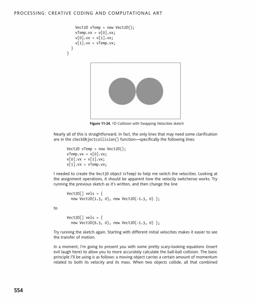
Vect2D vTemp = new Vect2D();vTemp.vx = v[0].vx;v[0].vx = v[1].vx;v[1].vx = vTemp.vx;
}}
Figure 11-24. 1D Collision with Swapping Velocities sketch
Nearly all of this is straightforward. In fact, the only lines that may need some clarificationare in the checkObjectcollision() function—specifically the following lines:
Vect2D vTemp = new Vect2D();vTemp.vx = v[0].vx;v[0].vx = v[1].vx;v[1].vx = vTemp.vx;
I needed to create the Vect3D object (vTemp) to help me switch the velocities. Looking atthe assignment operations, it should be apparent how the velocity switcheroo works. Tryrunning the previous sketch as it’s written, and then change the line
Vect2D[] vels = { new Vect2D(1.3, 0), new Vect2D(-1.3, 0) };
to
Vect2D[] vels = { new Vect2D(6.3, 0), new Vect2D(-1.3, 0) };
Try running the sketch again. Starting with different initial velocities makes it easier to seethe transfer of motion.
In a moment, I’m going to present you with some pretty scary-looking equations (insertevil laugh here) to allow you to more accurately calculate the ball-ball collision. The basicprinciple I’ll be using is as follows: a moving object carries a certain amount of momentumrelated to both its velocity and its mass. When two objects collide, all that combined
PROCESSING: CREATIVE CODING AND COMPUTATIONAL ART
554
617xCH11.qxd 4/17/07 1:57 PM Page 554

momentum at impact has to go somewhere. In the real world, the force of this impactturns into heat, sound, cool explosions, and new motion. In a virtual world, we can controlhow the force is transferred. For example, when two objects collide, if we force all themomentum upon impact to go back into only new motion, then somehow the motionafter the impact alone needs to be equal to the total momentum of the two objects at thepoint of impact. The easiest way to pull this off in code, as I did in the last example, is sim-ply to have the two objects exchange their velocities upon impact.
Less simple 1D collision This last example, although relatively simple, didn’t take into account the mass of theobjects. I used the term “transfer of motion” to describe how the balls simply switchedtheir velocities. But what if you want to account for balls of different mass? Introducingmass requires those scary equations I mentioned earlier. Again, here’s the first:
MOTION
555
11
obj 1 final velocity = (obj 1 mass – obj 2 mass) * obj 1 velocity + 2 * obj 2 mass * obj 2 velocity
------------------------------------------------------------------------------------------------------------------------------------
obj 1 mass + obj 2 mass
And here’s the second:
obj 2 final velocity = (obj 2 mass – obj 1 mass) * obj 2 velocity + 2 * obj 1 mass * obj 1 velocity
------------------------------------------------------------------------------------------------------------------------------------
obj 1 mass + obj 2 mass
I know the equations are long, but converting them to code is not a big deal, as you’ll seeshortly. The hard part of course would be attempting to derive the equations, which Iwon’t bother doing. Keith Peters’s book goes into some detail about where the equationscome from. If you’re really interested in the math, here’s a link you might enjoy as well:www.euclideanspace.com/physics/dynamics/collision/oned/index.htm.
The two equations are based on the law of conservation of momentum, which I’ve sort ofalready discussed. For our purposes, the law states that in a closed system (such as thetype we’re coding), the total momentum of objects before a collision is equal to the totalmomentum after the collision. By using these equations, you’ll be able to now account formass in your ball-ball collisions.
The next example, shown in Figure 11-25, requires only some minor tweaks to the previ-ous sketch. The sketch can be divided into five tabs like the last, with the main tab code,Vect2D class, and checkBoundaryCollision() function all remaining exactly as they werein the previous sketch, so I won’t bother repeating that code. All you need to do is updatethe Ball class and checkObjectCollision() function. Here’s the revised Ball class, withthe new changes displayed in bold:
617xCH11.qxd 4/17/07 1:57 PM Page 555

class Ball{float x, y, r, m;
// default constructorBall() {}
Ball(float x, float y, float r) {this.x = x;this.y = y;this.r = r;m = r*.1;
}}
If it isn’t obvious, all I added was a mass property to the class and based its value on theradius. Of course, the mass could also be coded as a completely separate value fromthe radius, as, for example, a large cork ball would certainly weigh less than a muchsmaller steel ball bearing. That being said, tying the mass to the radius was easiest.
The checkObjectCollision() function is where the majority of changes are, and of courseit’s where the scary conservation of momentum expressions are coded:
void checkObjectCollision(Ball[] b, Vect2D[] v){float d = dist(b[0].x, b[0].y, b[1].x, b[1].y);if (d < b[0].r + b[1].r){
/* calculate final velocities based onLaw of Conservation of Momentum */
float finalVel0 = ((b[0].m - b[1].m) * v[0].vx + 2 *!b[1].m * v[1].vx) / (b[0].m + b[1].m);
float finalVel1 = ((b[1].m - b[0].m) * v[1].vx + 2 *!b[0].m * v[0].vx) / (b[0].m + b[1].m);
v[0].vx = finalVel0;v[1].vx = finalVel1;
}}
Hopefully, you didn’t find the long expressions too frightening; they’re long but prettystraightforward, and of course there’s no obligation to really understand why they work(but then I’m not your Physics teacher). Following the new expressions, I simply assign thefinal velocities to the original velocity variables.
PROCESSING: CREATIVE CODING AND COMPUTATIONAL ART
556
617xCH11.qxd 4/17/07 1:57 PM Page 556

Figure 11-25. 1D Collision Using Conservation of Momentum sketch
Try running the sketch a few times and changing the radius of one of the balls. The greaterthe difference between the two radii, the more obvious the effect of the conservation ofmomentum will be.
2D collisionsNow that we got most of the easy stuff over with (I’m winking, don’t worry), we’ll tacklethe holy grail of collisions: non-orthogonal 2D collisions. In actuality, you already knowhow to do this (well, sort of). I’ll be using the same coordinate rotation approach I used forthe Asteroid Shower sketch. The main difference is that there are now two objects collid-ing (shown in Figure 11-26).
The main sketch tab reuses much of the existing code from the previous example, with thechanges shown in bold, as follows:
// Main Sketch Tab// 2D Collision Using Conservation of MomentumBall[] balls = { new Ball(100, 400, 10), new Ball(700, 400, 40) };
Vect2D[] vels = { new Vect2D(4.3, -2.7), new Vect2D(-3.3, .95) };
void setup(){size(400, 400);smooth();noStroke();
}
void draw(){background(255);fill(150);for (int i=0; i<2; i++){balls[i].x += vels[i].vx;balls[i].y += vels[i].vy;
MOTION
557
11
617xCH11.qxd 4/17/07 1:57 PM Page 557

ellipse(balls[i].x, balls[i].y, balls[i].r*2, balls[i].r*2);checkBoundaryCollision(balls[i], vels[i]);
}checkObjectCollision(balls, vels);
}
The checkObjectCollision() function needs a few more changes than that; here it is(brace yourself):
void checkObjectCollision(Ball[] b, Vect2D[] v){
// get distances between the balls' componentsVect2D bVect = new Vect2D();bVect.vx = b[1].x - b[0].x;bVect.vy = b[1].y - b[0].y;
// calculate magnitude of the vector separating the ballsfloat bVectMag = sqrt(bVect.vx * bVect.vx + bVect.vy * bVect.vy);if (bVectMag < b[0].r + b[1].r){// get angle of bVectfloat theta = atan2(bVect.vy, bVect.vx);// precalculate trig valuesfloat sine = sin(theta);float cosine = cos(theta);
/* bTemp will hold rotated ball positions. You just need to worry about bTemp[1] position*/
Ball[] bTemp = { new Ball(), new Ball() };/* b[1]'s position is relative to b[0]'sso you can use the vector between them (bVect) as the reference point in the rotation expressions.bTemp[0].x and bTemp[0].y will initializeautomatically to 0.0, which is what you wantsince b[1] will rotate around b[0] */bTemp[1].x = cosine * bVect.vx + sine * bVect.vy;bTemp[1].y = cosine * bVect.vy - sine * bVect.vx;
// rotate Temporary velocitiesVect2D[] vTemp = { new Vect2D(), new Vect2D() };vTemp[0].vx = cosine * v[0].vx + sine * v[0].vy;vTemp[0].vy = cosine * v[0].vy - sine * v[0].vx;vTemp[1].vx = cosine * v[1].vx + sine * v[1].vy;vTemp[1].vy = cosine * v[1].vy - sine * v[1].vx;
/* Now that velocities are rotated, you can use 1Dconservation of momentum equations to calculate the final velocity along the x-axis. */Vect2D[] vFinal = { new Vect2D(), new Vect2D() };// final rotated velocity for b[0]
PROCESSING: CREATIVE CODING AND COMPUTATIONAL ART
558
617xCH11.qxd 4/17/07 1:57 PM Page 558

vFinal[0].vx = ((b[0].m - b[1].m) * vTemp[0].vx + 2 * b[1].m *vTemp[1].vx) / (b[0].m + b[1].m);
vFinal[0].vy = vTemp[0].vy;// final rotated velocity for b[0]vFinal[1].vx = ((b[1].m - b[0].m) * vTemp[1].vx + 2 * b[0].m *vTemp[0].vx) / (b[0].m + b[1].m);
vFinal[1].vy = vTemp[1].vy;
// hack to avoid clumpingbTemp[0].x += vFinal[0].vx;bTemp[1].x += vFinal[1].vx;
/* Rotate ball positions and velocities backReverse signs in trig expressions to rotate in the opposite direction */// rotate ballsBall[] bFinal = { new Ball(), new Ball() };bFinal[0].x = cosine * bTemp[0].x - sine * bTemp[0].y;bFinal[0].y = cosine * bTemp[0].y + sine * bTemp[0].x;bFinal[1].x = cosine * bTemp[1].x - sine * bTemp[1].y;bFinal[1].y = cosine * bTemp[1].y + sine * bTemp[1].x;
// update balls to screen positionb[1].x = b[0].x + bFinal[1].x;b[1].y = b[0].y + bFinal[1].y;b[0].x = b[0].x + bFinal[0].x;b[0].y = b[0].y + bFinal[0].y;
// update velocitiesv[0].vx = cosine * vFinal[0].vx - sine * vFinal[0].vy;v[0].vy = cosine * vFinal[0].vy + sine * vFinal[0].vx;v[1].vx = cosine * vFinal[1].vx - sine * vFinal[1].vy;v[1].vy = cosine * vFinal[1].vy + sine * vFinal[1].vx;
}}
Figure 11-26. 2D Collision Using Conservation of Momentum sketch
MOTION
559
11
617xCH11.qxd 4/17/07 1:57 PM Page 559

OK, hopefully we’re still on speaking terms. Part of the reason this function is so long, witha slew of temporary object arrays, is that I wanted to make all the processes as explicit aspossible. There are many ways of optimizing this code and reducing the number of lines;however, that economy comes with a cost of potential confusion. (Again, Keith Peters’sbook discusses a bunch of these optimizations, so I encourage you to take a look at it fora deeper discussion on this topic.)
I added a lot of comments directly within the code to help you decipher it. In addition, I’llprovide a brief overview.
The code in the function combines a number of concepts we’ve looked at throughout thischapter, including vectors, coordinate rotation, and of course the law of conservation ofmomentum. I began the function by assigning the vector described by the distance betweenthe two balls to bVect. I used this vector to determine the angle of rotation between theballs, as well as to define the reference point for rotation. Vectors, you’ll remember, tell usabout both direction and magnitude. I calculated the magnitude of bVect (assigned tobVectMag) and used it to determine when the balls were colliding, since the vectorbetween the balls is also conveniently the distance between the balls.
By plugging the components of bVect into the atan2() function, I was able to find theangle (in radians) of the vector’s rotation, which is precisely the value you need to rotatethe ball and velocity coordinates, allowing you to treat the 2D collision between the ballsas a 1D (orthogonal) collision.
When rotating the ball and velocity coordinates, you don’t want to rotate in reference tothe screen origin, but rather locally around the point of collision. I accomplished this byusing bVect (the vector describing the distance between the balls) as the reference pointof rotation. The two lines I’m referring to are the following (please note that I created abunch of temporary Ball and Vect2D arrays (including bTemp) in the function to try tohelp clarify the different steps in the collision process):
bTemp[1].x = cosine * bVect.vx + sine * bVect.vy;bTemp[1].y = cosine * bVect.vy - sine * bVect.vx;
b[1] will rotate around b[0], setting the vector between them perfectly horizontal. Thus,b[0] will act, in a sense, as the origin for the rotation, so I don’t need to assign any valueto bTemp[0].x and bTemp[0].y, which were both automatically assigned 0.0 whenbTemp[0] was instantiated (since float values—which the x and y properties are—defaultto 0.0 when declared).
Next, I rotated the velocities, which should be self-explanatory, using the good old longform trig expressions.
The rotated velocities were assigned to the vTemp objects. Next, the ugly conservation ofmomentum expressions come into play. Notice that I only used them to find the finalrotated velocities along the x-axis. The velocities along the y-axis were calculated previ-ously, so I simply assigned vTemp.vy to vFinal.vy (for both objects).
PROCESSING: CREATIVE CODING AND COMPUTATIONAL ART
560
617xCH11.qxd 4/17/07 1:57 PM Page 560

To avoid unintentional clumping of the balls at collision, I borrowed a nice hack fromKeith’s example, which essentially moves the balls a little away from each other upon col-lision detection so that clumping is avoided. It’s not a perfect fix, but it sure is nice andsimple.
We’re almost home now. The last steps left are to rotate the rotated ball position valuesand velocities back to the original rotation at collision and to update the balls’ positions tothe screen (remember that I treated the rotation locally with regard to the vector betweenthe balls, rotating b[1] around b[0]). Updating the balls’ screen positions just entailsadding the final ball positions (bFinal) to b[0].
That’s it! Definitely take some time playing with this sketch, plugging in different values forthe balls’ radii (which, again, control mass) and the initial velocities, both defined in thesketch’s main tab.
There is so much more that could be done with this sketch, and collisions in general,including the addition of more balls. Likewise, orb-orb collisions could also be introducedto the Asteroid Shower example. That being said, I think this chapter’s gone on longenough.
SummaryThis chapter began with a brief overview of some of the technical issues involved in com-puter-based animation, including the concept of threads and the use of timeline-basedkeyframe models commonly found in high-end animation applications. Comparing Javaand Processing animation code side by side, I showed how Processing’s draw() structureencapsulates much of the low-level (and annoying) aspects of programmatic animation.Beginning with a simple moving ball and eventually adding simple physics, you exploredeasing, springing, and the concept of soft-body dynamics. Coding collisions, with somehelp from code guru Keith Peters, I introduced different approaches for handling bothorthogonal and non-orthogonal 1D collisions, including ways to work with multiple sur-faces and objects. Finally, I introduced an advanced 2D collision example that includedconservation of momentum calculations.
In the next chapter, we’ll add interactivity into the mix, allowing the user to interact withyour sketches. We’ll also discuss the possibilities of generating applications and graphicaluser interfaces (GUIs) in Processing.
MOTION
561
11
617xCH11.qxd 4/17/07 1:57 PM Page 561

617xCH12.qxd 4/20/07 2:22 PM Page 562

12 INTERACTIVITY
617xCH12.qxd 4/20/07 2:22 PM Page 563

One of the most compelling aspects of digital/code art is interactivity. Interactive art is notin itself a completely new concept—for example, we’ve all become quite accustomed to“please touch” type children’s museums. However, what is unique in code art is the factthat users can not only interact with a work of art, but in some cases they can actuallyredefine it, or even use the piece of art to create their own original works of art. MarkNapier’s piece net.flag (www.guggenheim.org/internetart/welcome.html) is an excellentexample of this. Viewers use Napier’s web-based piece to design a flag, which (conceptu-ally) becomes the flag of the entire Internet. Their creation remains the current flag of theNet until another viewer changes it. Each of the flags created also gets put into a perma-nent viewable database. Napier’s piece—and others like it—represents a radical breakwith the established view of a work of art as contemplative object/space. Instead, in thecase of net.flag, the work of art almost disappears, becoming a dynamic tool that otherscan use to express themselves.
In this chapter, you’ll learn how to both detect and handle events. By events, I mean inputsto the system, such as mouse clicks or key presses. Of course, there are events that occurat a lower-level than the graphical user interface (GUI), as well—such as an internal timeror other system process that communicates with a running application. For example, mymail program periodically checks for incoming mail without my having to request it. It’salso possible to detect other less standard high-level events, such as input from a videocamera, microphone, or motion sensor. Processing has the capacity to interface with allthese types of events. While in this chapter I’ll only be covering mouse and key events, theprinciples discussed apply to most input devices.
Interactivity simplifiedAs you’ve probably come to expect by now, Processing simplifies the process ofinteractivity by encapsulating a bunch of the code you’d be required to include using pureJava. For an example of this, take a look at the following three sketches, each of whichfunctions identically. The first two are written in Java and the third in Processing, but allthree can be run in Processing. When run, the sketches print to the text area in theProcessing application when the mouse is pressed within the Processing display window.
// 2 different Java approaches// Java approach 1 implements the Java MouseListener interface:void setup(){new MouseEventDemo();
}class MouseEventDemo implements MouseListener {//constructorMouseEventDemo(){addMouseListener(this);
}// we're required to implement all MouseListener methodspublic void mousePressed(MouseEvent e) {println("Java MouseListener interface example"+ !
"mouse press detected");
PROCESSING: CREATIVE CODING AND COMPUTATIONAL ART
564
617xCH12.qxd 4/20/07 2:22 PM Page 564

}public void mouseClicked(MouseEvent e){}public void mouseEntered(MouseEvent e){}public void mouseExited(MouseEvent e){}public void mouseReleased(MouseEvent e){}
}
// Java approach 2 extends the Java MouseAdapter classvoid setup(){new MouseEventDemo();
}class MouseEventDemo extends MouseAdapter {//constructorMouseEventDemo(){addMouseListener(this);
}public void mousePressed(MouseEvent e) {println("Java MouseAdapter class example: mouse press detected");
}}
// Processing "easy" approachvoid draw(){} // we're required to include draw() functionvoid mousePressed() {println("Processing example: mouse press detected");
}
The two Java approaches are both more complex and require more code than theProcessing approach. Using Java’s MouseAdapter class simplifies things somewhat, as theMouseAdapter class encapsulates the necessary implementation of all the requiredMouseListener methods. The Processing approach takes this concept of encapsulationone step further, making it unnecessary to explicitly implement or extend another mouseevent–related interface or class. In reality, the Processing approach I wrote is a little toolean, as you’d almost always want to include Processing’s setup() function as well asdraw(). However, all that is technically required for the mouse event detection to work inProcessing is the inclusion of the draw() function.
Mouse eventsBesides mouse press detection, Processing also includes event detection for mousereleases, clicks, moves, and drags. Mouse release detection occurs whenever the mousebutton is released, regardless if the mouse position changes while the mouse is pressed. Incomparison, mouse click detection occurs only if the mouse is released at the same pointit was pressed. When the mouse is pressed and released at the same point, both releaseand then click detection occur—always in this order. Mouse move detection occurs whenthe mouse moves, without the mouse button being pressed, while mouse dragging detec-tion occurs while the mouse moves with the button pressed. In addition, Processing can
INTERACTIVITY
565
12
617xCH12.qxd 4/20/07 2:22 PM Page 565

detect which mouse button is pressed (left, right, or center), using Processing’smouseButton system variable. With a little help from Java, it can also detect multiple but-ton clicks, which I’ll illustrate in a sketch at the end of the chapter.
Following is a better mouse event example, in which a rectangle on the screen is moved tothe position of the mouse when the mouse button is pressed. The mouseX and mouseYproperties are used to get the respective x and y positions of the mouse.
// mousePressed function// example 1
// declare x, yfloat x, y;// declare and initialize w, hfloat w = 20.0, h = 20.0;
void setup(){size(400, 400);// initialize x, yx = width/2.0;y = height/2.0;rectMode(CENTER);
}
void draw(){background(255);rect(x, y, w, h);
}
void mousePressed() {x = mouseX;y = mouseY;
}
This example utilizes a function called mousePressed(). Remember, the void in front ofthe function identifier just means that the function doesn’t return a value. Processing alsoprovides an alternative mousePressed Boolean variable that detects whether the mouse ispressed. The variable is equal to true if the mouse is pressed and false if it’s not. As thefollowing code shows, the previous sketch can be easily changed to use the mousePressedvariable instead of the mousePressed() function:
// mousePressed variable// example 2
// declare x, yfloat x, y;// declare and initialize w, hfloat w = 20.0, h = 20.0;
PROCESSING: CREATIVE CODING AND COMPUTATIONAL ART
566
617xCH12.qxd 4/20/07 2:22 PM Page 566

void setup(){size(400, 400);// initialize x, yx = width/2.0;y = height/2.0;rectMode(CENTER);
}
void draw(){background(255);rect(x, y, w, h);
if (mousePressed){x = mouseX;y = mouseY;
}}
This may seem confusing if you’re a new coder—why have two ways of doing the samething? Well, if you run this last example, you’ll notice that the two sketches actually don’trun quite the same way. This last example updates the rectangle’s x and y positions con-tinuously while the mouse is pressed, allowing the rectangle to be dragged in the displaywindow. The earlier example only updated the rectangle when the mouse was pressed. Asyou look at some more complex examples, it will become clearer how these twoapproaches differ.
Notice also when I checked the condition (true or false) of the mousePressed Booleanvariable, I just included it between the parentheses: (mousePressed). I didn’t explicitlycheck if it was true using (mousePressed == true). This shortcut is perfectly legal, sincethe Boolean value will evaluate to either true or false, which is what the if statementneeds to know in determining whether it should execute the code between its curlybraces.
In addition to mouse press events, you can detect mouse release events. Here’s anexample:
// mouseReleased// example 1
// declare x, yfloat x, y;// declare and initialize w, hfloat w = 20.0, h = 20.0;// rectangle fill color variablecolor rectColor = color(255, 255, 255);
void setup(){size(400, 400);// initialize x, yx = width/2.0;
INTERACTIVITY
567
12
617xCH12.qxd 4/20/07 2:22 PM Page 567

y = height/2.0;rectMode(CENTER);
}
void draw(){background(255);fill(rectColor);rect(x, y, w, h);
}
void mousePressed() {x = mouseX;y = mouseY;
}
// randomly change fill color upon mouse releasevoid mouseReleased() {rectColor = color(random(255), random(255), random(255));
}
In this example, I included the original mousePressed() function and added amouseReleased() function. When you run the sketch, you’ll see that Processing can detectboth parts of the mouse click (the press and release) as separate events. ThemouseReleased() function creates a random color for the rectangle’s fill.
The mouseMoved() and mouseDragged() functions work similarly to mousePressed() andmouseReleased(). Here’s a mouseDragged() example:
// mouseDragged Examplefloat x, y;// declare and initialize radiusfloat r = 5.0;
void setup(){size(400, 400);
If you’re a detail-oriented person (I’m really not), you may have noticed some incon-sistency with Processing’s automatic syntax color highlighting in the text editor. Ingeneral, Processing’s built-in functions turn orange, while built-in variables turn red.However, the mousePressed() function turns red, and the mouseClicked() functionremains black. The other mouse event functions, mouseReleased(), mouseMoved(),and mouseDragged(), turn orange. This is definitely confusing, and I’ve seen com-ments on the Processing discussion board saying so as well. Perhaps at some point thisminor issue will be addressed; for now, just realize that it’s not something you’re doingwrong, and that the color of your code in the text editor has no effect on the func-tionality of the code. (It’s also possible that by the time you read this, the issue willhave been resolved.)
PROCESSING: CREATIVE CODING AND COMPUTATIONAL ART
568
617xCH12.qxd 4/20/07 2:22 PM Page 568

// initialize x, yx = width/2.0;y = height/2.0;frameRate(30);smooth();noStroke();
}
void draw(){// fading backgroundfill(0, 5);rect(0, 0, width, height);
fill(255);ellipse(x, y, r*2, r*2);
}
void mouseDragged() {x = mouseX;y = mouseY;
}
This example works similarly to the earlier mousePressed Boolean variable example. Whenyou press the mouse in the display window and drag, the ellipse follows the mouse.
The next example adds a mouseMoved() function that controls a jitter and a scattervariable, which are set as you move the mouse around the display window (without itbeing pressed). The scatter variable controls the limit on a for loop, while the jittervariable controls the radius on a ring of random ellipses created in the for loop. Upondragging the mouse (i.e., with the button pressed), the ring of ellipses will follow the cur-sor using the last jitter and scatter settings set. This is because mouse dragging andmouse moving, similarly to the press and release events, are processed as unique mouseevent states—you can’t press and release at the same time, nor can you move and drag atthe same time.
// mouseMoved Examplefloat x, y;// declare and initialize radiusfloat r = 1.5;float jitter = 5;float scatter = 1;
void setup(){size(400, 400);// initialize x, yx = width/2.0;y = height/2.0;frameRate(30);smooth();noStroke();
INTERACTIVITY
569
12
617xCH12.qxd 4/20/07 2:22 PM Page 569

}
void draw(){// fading backgroundfill(0, 5);rect(0, 0, width, height);
fill(255);for (int i=0; i<scatter; i++){float angle = random(TWO_PI);float sctterDistX = x+cos(angle)*jitter;float sctterDistY = y+sin(angle)*jitter;ellipse(sctterDistX, sctterDistY, r*2, r*2);
}}
void mouseDragged() {x = mouseX;y = mouseY;
}
// scatter/jitter ellipsevoid mouseMoved() {scatter = mouseX*.05;jitter = mouseY*.05;
}
The next example, shown in Figure 12-1, combines mouse events with some of the motionprinciples covered in Chapter 11. I think you’ll find this next sketch more aestheticallyinteresting than the “learning” examples you’ve looked at thus far in this chapter—butyou’ve got to crawl some before you dance! This sketch allows you to plot points, ornodes, that get connected with lines. After three or more nodes are plotted, you can clickback on the initial plotted node and close the shape. Once the shape is closed, some coolstuff happens. Here’s the code:
// Shape Builder and Animator Examplefloat nodeRadius = 5.0;// holds node coordinate valuesfloat[]nodeXPos = new float[0];float[]nodeYPos= new float[0];
color initialNode = color(0);boolean isShapeClosed = false;
//dynamics variables (moves shape)float gravity = .95;float jitterRange = 5;float elasticRangeMin = .75;float elasticRangeMax = .95;
PROCESSING: CREATIVE CODING AND COMPUTATIONAL ART
570
617xCH12.qxd 4/20/07 2:22 PM Page 570

float friction = .85;float[]jitter = new float[0];float[]xSpeed = new float[0];float[]ySpeed = new float[0];float[]elasticity = new float[0];
void setup(){size(400, 600);frameRate(30);smooth();
}
void draw(){// create simple shape trailsfill(255, 36);rect(0, 0, width, height);
if (nodeXPos.length>1){// draw line between nodesdrawEdge();// check if mouse is over original nodecheckOverInitialNode();// animate shapemoveShape();
}// draw nodedrawNode();
}
// change node fill color when mouse is over initial nodevoid checkOverInitialNode(){if (isInitialNode()){initialNode = color(255, 127, 0);
}else {initialNode = color(0);
}}
//function to draw lines between nodesvoid drawEdge(){stroke(100, 50, 20);for (int i=0; i<nodeXPos.length; i++){if (i>0){line(nodeXPos[i], nodeYPos[i], nodeXPos[i-1], nodeYPos[i-1]);
}// close shape, line between last node and initial nodeif (isShapeClosed && i == nodeXPos.length-1){line(nodeXPos[i], nodeYPos[i], nodeXPos[0], nodeYPos[0]);
INTERACTIVITY
571
12
617xCH12.qxd 4/20/07 2:22 PM Page 571

}}
}
// function to draw nodesvoid drawNode(){// draw nodes at shape verticesnoStroke();for (int i=0; i<nodeXPos.length; i++){// initial node has own color variableif (i==0){fill(initialNode);
}else{fill(0);
}ellipse(nodeXPos[i], nodeYPos[i], nodeRadius*2, nodeRadius*2);
}}
// function returns true/false if mouse is over initial nodeboolean isInitialNode(){boolean isOnNode = false;if (nodeXPos.length>2){if (dist(mouseX, mouseY, nodeXPos[0], nodeYPos[0]) < nodeRadius){isOnNode = true;
}}return isOnNode;
}
void mousePressed(){if(isShapeClosed){// after shape is closed empty arraysnodeXPos = subset(nodeXPos, 0, 0);nodeYPos = subset(nodeYPos, 0, 0);xSpeed = subset(xSpeed, 0, 0);ySpeed = subset(ySpeed, 0, 0);jitter = subset(jitter, 0, 0);elasticity = subset(elasticity, 0, 0);
//reset variable to falseisShapeClosed = false;
}
if(!isInitialNode()){// if not on initial node plot at mouse position// increase size of node coordinate arraysnodeXPos = append(nodeXPos, mouseX);
PROCESSING: CREATIVE CODING AND COMPUTATIONAL ART
572
617xCH12.qxd 4/20/07 2:22 PM Page 572

nodeYPos = append(nodeYPos, mouseY);
// increase size of dynamics arraysxSpeed = append(xSpeed, 0);jitter = append(jitter, random(-jitterRange, jitterRange));elasticity = append(elasticity, random(elasticRangeMin, !
elasticRangeMax));ySpeed = append(ySpeed, 0);
}else {// set to true to avoid additional nodes on shapeisShapeClosed = true;
}}
//function to move shapevoid moveShape(){//animate after shape is closedif (isShapeClosed){for (int i=0; i<nodeXPos.length; i++){nodeXPos[i]+=xSpeed[i];ySpeed[i]+=gravity;nodeYPos[i]+=ySpeed[i];
// set display window edge collision// right display window edgeif (nodeXPos[i]>width-nodeRadius){nodeXPos[i] = width-nodeRadius;xSpeed[i]*=-1;
}// left display window edgeif (nodeXPos[i]<nodeRadius){nodeXPos[i] = nodeRadius;xSpeed[i]*=-1;
}
// bottom display window edgeif (nodeYPos[i]>height-nodeRadius){nodeYPos[i] = height-nodeRadius;xSpeed[i]+=jitter[i];xSpeed[i]*=friction;jitter[i]*=friction;ySpeed[i]*=-1;ySpeed[i]*=elasticity[i];
}}
}}
INTERACTIVITY
573
12
617xCH12.qxd 4/20/07 2:22 PM Page 573

Figure 12-1. Shape Builder and Animator Example sketch
You should play with this sketch some to see what it can do. Besides running the sketch, Ialso recommend messing with some of the variable values declared at the top of theprogram.
To give you a better understanding, I’ll now go over the sketch a section at a time.
// Shape Builder and Animator Examplefloat nodeRadius = 5.0;// holds node coordinate valuesfloat[]nodeXPos = new float[0];float[]nodeYPos= new float[0];
color initialNode = color(0);boolean isShapeClosed = false;
//dynamics variables (moves shape)float gravity = .95;float jitterRange = 5;float elasticRangeMin = .75;float elasticRangeMax = .95;float friction = .85;float[]jitter = new float[0];float[]xSpeed = new float[0];float[]ySpeed = new float[0];float[]elasticity = new float[0];
PROCESSING: CREATIVE CODING AND COMPUTATIONAL ART
574
617xCH12.qxd 4/20/07 2:22 PM Page 574

As usual, I declare global variables at the top of the program, before the setup() function.The nodeXPos[] and nodeYPos[] arrays hold the shape coordinate data as the shapes areplotted. The initialNode color variable is used to dynamically set a color on the initialplotted node when it is moused over—this functions like a rollover effect. (Later in thechapter, I’ll look at more examples of custom interactive buttons in Processing.) TheBoolean variable isShapeClosed maintains the status of the closed state of the shape,which is important, as animation only occurs when this variable is true. The dynamics vari-ables (most of which were discussed in Chapter 11) handle the animation. Many of thevariables are arrays, since animation is applied to each individual node. Since it’s notknown how many nodes will be plotted for each shape, these arrays are initialized withzero length. Later in the sketch, as the user plots a node, values (and length) are added tothe array using Processing’s append() function.
void setup(){size(400, 600);frameRate(30);smooth();
}
The setup() function is nice and simple—hopefully, it doesn’t need any explanation.
void draw(){// create simple shape trailsfill(255, 36);rect(0, 0, width, height);
if (nodeXPos.length>1){// draw line between nodesdrawEdge();// check if mouse is over original nodecheckOverInitialNode();// animate shapemoveShape();
}// draw nodedrawNode();
}
The draw() function is relatively simple as well, considering the amount of stuff happeningin this sketch. By creating some custom functions, I was able to keep the draw()function pretty lean. I wrapped the three custom function calls (drawEdge(),checkOverInitialNode(), and moveShape()) in a conditional block to ensure that at leasttwo nodes are plotted prior to connecting the nodes with lines. drawEdge() calls a func-tion that handles the drawing of the lines between the nodes. I called this function prior toactually drawing the nodes so that the nodes appear on top of the connecting lines.checkOverInitialNode() checks if the mouse is over the initial node, allowing the colorof the node to be changed. moveShape() animates the shape after it’s closed. Below theconditional block, I called drawNode(), which, as you might suspect, draws the nodes.
INTERACTIVITY
575
12
617xCH12.qxd 4/20/07 2:22 PM Page 575

void checkOverInitialNode(){if (isInitialNode()){initialNode = color(255, 127, 0);
}else {initialNode = color(0);
}}
The checkOverInitialNode() function sets the color variable initialNode to orangewhen the mouse hovers over the initial node, and then resets it to black when the mousemoves off the node.
void drawEdge(){stroke(100, 50, 20);for (int i=0; i<nodeXPos.length; i++){if (i>0){line(nodeXPos[i], nodeYPos[i], nodeXPos[i-1], nodeYPos[i-1]);
}// close shape, line between last node and initial nodeif (isShapeClosed && i == nodeXPos.length-1){line(nodeXPos[i], nodeYPos[i], nodeXPos[0], nodeYPos[0]);
}}
}
drawEdge() draws a line connecting the plotted nodes. The for loop is controlled by thelength of the nodeXPos[] array, which increases each time a new node is plotted. The con-ditional blocks nested within the for loop ensure that lines are drawn only when there areat least two nodes plotted, and that the final line connects the last plotted node with theinitial node, closing the shape.
void drawNode(){// draw nodes at shape verticesnoStroke();for (int i=0; i<nodeXPos.length; i++){// initial node has own color variableif (i==0){fill(initialNode);
}else{fill(0);
}ellipse(nodeXPos[i], nodeYPos[i], nodeRadius*2, nodeRadius*2);
}}
drawNode() draws the nodes using Processing’s ellipse() function and the coordinatevalues stored in the nodeXPos[] and nodeYPos[] arrays. The conditional if...else blockfills the initial node’s color using the intialNode color variable, while all the other nodes
PROCESSING: CREATIVE CODING AND COMPUTATIONAL ART
576
617xCH12.qxd 4/20/07 2:22 PM Page 576

are filled with black. Using the intialNode variable allows the first plotted node’s color tobe changed when the mouse is over it, providing some interactive direction to the user.
// function returns true/false if mouse is over initial nodeboolean isInitialNode(){boolean isOnNode = false;if (nodeXPos.length>2){if (dist(mouseX, mouseY, nodeXPos[0], nodeYPos[0]) < nodeRadius){isOnNode = true;
}}return isOnNode;
}
The isInitialNode() function returns true if there are more than two nodes plotted andthe mouse is over the initially plotted node. If neither of these conditions is true, the func-tion returns false. Notice how I declared the function using the boolean keyword in frontof the function name; this enforces that the function must return a Boolean value. Notealso that the Boolean variable isOnNode, which I declared within the function, only existslocally (has local scope) within the function.
void mousePressed(){if(isShapeClosed){// after shape is closed empty arraysnodeXPos = subset(nodeXPos, 0, 0);nodeYPos = subset(nodeYPos, 0, 0);xSpeed = subset(xSpeed, 0, 0);ySpeed = subset(ySpeed, 0, 0);jitter = subset(jitter, 0, 0);elasticity = subset(elasticity, 0, 0);
//reset variable to falseisShapeClosed = false;
}
if(!isInitialNode()){// if not on initial node plot at mouse position// increase size of node coordinate arraysnodeXPos = append(nodeXPos, mouseX);nodeYPos = append(nodeYPos, mouseY);
// increase size of dynamics arraysxSpeed = append(xSpeed, 0);jitter = append(jitter, random(-jitterRange, jitterRange));elasticity = append(elasticity, random(elasticRangeMin, !
elasticRangeMax));ySpeed = append(ySpeed, 0);
}else {// set to true to avoid additional nodes on shape
INTERACTIVITY
577
12
617xCH12.qxd 4/20/07 2:22 PM Page 577

isShapeClosed = true;}
}
The mousePressed() function begins with a conditional block that initializes the sketcharrays when the shape is closed; this allows new shapes to be plotted when the mouse ispressed (only after the shape has been closed and has begun animating). I usedProcessing’s subset() function to reset the primitive arrays. The function returns a subsetof an array. The first argument is the array to subset, the second argument is the place inthe array to begin the subset, and the third argument is the number of positions in thearray to include in the subset. Since I used 0, 0 for the starting point and number of posi-tions in the subset, an empty array was returned. Notice that I assigned the empty arrayback to the same array I used in the first argument; this may look odd, but it is perfectlylegal. At the end of the conditional block, I reset the variable isShapeClosed to false toallow new nodes to be plotted.
The next conditional block, if(!isInitialNode()), uses the ! operator with the functioncall isInitialNode(). The function call returns a Boolean value (true or false). Prefacingthe function call with the exclamation mark means that the conditional test will evaluateto true when the function call returns false (i.e., when the user is not pressing on the ini-tial node). This kind of logic can hurt your head. Instead of using !isInitialNode(), youcould also use isInitialNode() == false or isInitialNode() != true to handle thetest.
Within the conditional block, I used Processing’s append() function. This functionincreases the length of arrays. The function takes two arguments: the first argument is thearray to append to, and the second is the value to add to the array. Like subset(),the append() function returns the changed array, which I reassigned to the same arrayvariable. On each mouse press, all six of the arrays are appended to. Finally, if the userclicks the initial node, the arrays are not expanded, but the Boolean variableisShapeClosed is set to true.
void moveShape(){//animate after shape is closedif (isShapeClosed){for (int i=0; i<nodeXPos.length; i++) {nodeXPos[i]+=xSpeed[i];ySpeed[i]+=gravity;nodeYPos[i]+=ySpeed[i];
// set display window edge collision// right display window edgeif (nodeXPos[i]>width-nodeRadius){nodeXPos[i] = width-nodeRadius;xSpeed[i]*=-1;
}// left display window edgeif (nodeXPos[i]<nodeRadius){nodeXPos[i] = nodeRadius;xSpeed[i]*=-1;
PROCESSING: CREATIVE CODING AND COMPUTATIONAL ART
578
617xCH12.qxd 4/20/07 2:22 PM Page 578

}
// bottom display window edgeif (nodeYPos[i]>height-nodeRadius){nodeYPos[i] = height-nodeRadius;xSpeed[i]+=jitter[i];xSpeed[i]*=friction;jitter[i]*=friction;ySpeed[i]*=-1;ySpeed[i]*=elasticity[i];
}}
}}
The final function in the sketch, moveShape(), controls the movement of the shape. Inested all the motion code in the conditional block (isShapeClosed), which evaluates totrue only if the shape is closed. The actual motion code should look familiar, as similarcode was covered in Chapter 11. The for loop ensures that speed values are added toeach of the shape’s nodes (the lines connecting the nodes rely on the nodes’ coordinatesfor their placement), and the collision code makes each node bounce off the sides andbottom of the display window. The animation uses gravity and jitter, which simulate theshape falling with acceleration and deflecting off an irregular ground surface. The arrayvariables elasticity[] and friction[] eventually bring the individual nodes to a stop atthe bottom of the display window.
Adding interface elementsNext, I’ll look at creating more elaborate interface elements, such as interactive buttons.Processing doesn’t come with any native prebuilt buttons, but you can easily build them,as I sort of did in the last example when I tested if the mouse was pressed on the initiallyplotted node. The only difference between detecting a mouse event on a button anddetecting a mouse event on the entire display window is in the evaluation of the size ofthe bounded hit area (the area that detects the event). Of course, when building a userinterface, you generally want to give the user more control than they get by simply click-ing the screen.
When creating a button, you can use Processing’s drawing/text functions or import agraphic—I’ll discuss both approaches in this chapter. This first sketch creates a single but-ton that starts a simple animation of a rectangle moving across the screen:
// Start Button
// buttonfloat btnX, btnY, btnW, btnH;
// moving rectanglefloat x = 25;
INTERACTIVITY
579
12
617xCH12.qxd 4/20/07 2:22 PM Page 579

float y = 30;float w = 10;float h = w;float xSpeed = 0;
void setup(){size(600, 100);btnX = width/2;btnY = height-20;btnW = 50;btnH = 20;
}
void draw(){background(200);rectMode(CENTER);fill(250);stroke(150);rect(btnX, btnY, btnW, btnH);
fill(0);noStroke();rect(x, y, w, h);x+=xSpeed;
}
void mousePressed(){if (mouseX>btnX-btnW/2 && mouseX< btnX+btnW/2 && !
mouseY>btnY-btnH/2 && mouseY< btnY+btnH/2){xSpeed+=.2;
}}
In this sketch, each time the mouse is pressed on the rectangle at the bottom of thescreen, the smaller square’s speed increases by .02. The mouse detection is now workingbased on the bounds of the button. However, since no feedback is provided, the usermight not understand that the sketch is working (or even that the rectangle is supposed tobe a button). You could improve the sketch by giving the user some more visual cues, suchas changing the cursor icon during detected mouse events, adding different renderingstates to the button (up, over, and down), giving the button a label, and providing someoutput based on the current speed of the moving square. The following sketch is a modi-fied version of the last that handles these improvements in two steps. The new and alteredcode is shown in bold.
// Interactive Button (step 1)
// buttonfloat btnX, btnY, btnW, btnH;
PROCESSING: CREATIVE CODING AND COMPUTATIONAL ART
580
617xCH12.qxd 4/20/07 2:22 PM Page 580

color btnUpState = color(200, 200, 200);color btnOverState = color(200, 200, 50);color btnDownState = color(255, 150, 20);
color btnBackground = btnUpState;
// moving squarefloat x = 25;float y = 30;float w = 10;float h = w;float xSpeed = 0;
void setup(){size(600, 100);btnX = width/2;btnY = height-20;btnW = 50;btnH = 20;
}
void draw(){background(150);rectMode(CENTER);fill(btnBackground);stroke(100);rect(btnX, btnY, btnW, btnH);
fill(0);noStroke();rect(x, y, w, h);x+=xSpeed;
}
void mousePressed(){if (mouseX>btnX-btnW/2 && mouseX< btnX+btnW/2 && !
mouseY>btnY-btnH/2 && mouseY< btnY+btnH/2){xSpeed+=.2;btnBackground = btnDownState;
}}void mouseReleased(){
btnBackground = btnOverState;}
void mouseMoved(){if (mouseX>btnX-btnW/2 && mouseX< btnX+btnW/2 && !
mouseY>btnY-btnH/2 && mouseY< btnY+btnH/2){cursor(HAND);
INTERACTIVITY
581
12
617xCH12.qxd 4/20/07 2:22 PM Page 581

btnBackground = btnOverState;} else {cursor(ARROW);btnBackground = btnUpState;
}}
The sketch makes a little more sense visually now. Processing’s cursor(cursor icon)function makes it really easy to change the cursor icon. The different built-in icons areARROW, CROSS, HAND, MOVE, TEXT, and WAIT. Please note that once you change the cursoricon, the new icon will remain until you call the cursor(cursor icon) function again.
The final version of this sketch (shown in Figure 12-2) will make it even more user-friendly,and will also add a few more interface elements, such as buttons with labels.Unfortunately, making the sketch simpler for the user can mean more (potentially a lotmore) work for the coder. Creating ergonomically friendly interfaces requires a lot ofcode, especially when the language (like Processing) doesn’t rely on a set of prebuilt widg-ets (buttons, sliders, spinners, etc.).
// Final Interactive Button Example
// font used for button textPFont myFont;//buttonsfloat btn1X, btn1Y, btn1W, btn1H;float btn2X, btn2Y, btn2W, btn2H;float btn3X, btn3Y, btn3W, btn3H;
color btnUpState = color(200, 200, 200);color btnOverState = color(200, 200, 50);color btnDownState = color(255, 150, 20);
color btn1Background = btnUpState;color btn2Background = btnUpState;
// moving squarefloat x = 25;float w = 10;float h = w;// randomly place square y position on screenfloat y = random(h/2, 70);
Please note that the following Final Interactive Button Example sketch requires thatthe Processing font Verdana-10.vlw be installed in the sketch’s data directory. Youcan create the font yourself by using Processing’s Create Font command, found underthe Tools menu, or you can download the font from the Download section on thefriends of ED web site (www.friendsofed.com/downloads.html).
PROCESSING: CREATIVE CODING AND COMPUTATIONAL ART
582
617xCH12.qxd 4/20/07 2:22 PM Page 582

float xSpeed = 0;color movingSquareBackground = color(random(255), !
random(255), random(255));
//controls mouse trailsboolean isTrailable = false;// mouse trails check boxboolean isTrailsSelected = false;
void setup(){size(600, 100);// load font from within the sketch's data directorymyFont = loadFont("Verdana-10.vlw");textFont(myFont, 10);
//buttons//speed- buttonbtn1X = 250;btn1Y = height-20;btn1W = 50;btn1H = 20;
//speed+ buttonbtn2X = width-250;btn2Y = height-20;btn2W = 50;btn2H = 20;
// check box controls mouse trailsbtn3X = width-60;btn3Y = height-20;btn3W = 10;btn3H = 10;
}
void draw(){rectMode(CENTER);
// mouse trailsif (isTrailable){fill(150, 16);rect(width/2, height/2, width, height);
}else {background(150);
}
stroke(100);//btn 1 - decreases speed
INTERACTIVITY
583
12
617xCH12.qxd 4/20/07 2:22 PM Page 583

fill(btn1Background);rect(btn1X, btn1Y, btn1W, btn1H);fill(75);text("speed -", btn1X-17, btn1Y+btn1H/4);
//btn2 - increases speedfill(btn2Background);rect(btn2X, btn2Y, btn2W, btn2H);fill(75);text("speed +", btn2X-17, btn2Y+btn2H/4);
//btn3 - check box controls mouse trailsfill(255);rect(btn3X, btn3Y, btn3W, btn3H);fill(75);text("trails", btn3X+10, btn3Y+btn3H/4);if (isTrailsSelected){// draw x in boxline(btn3X-btn3W/2, btn3Y-btn3H/2, btn3X+btn3W/2, btn3Y+btn3H/2);line(btn3X-btn3W/2, btn3Y+btn3H/2, btn3X+btn3W/2, btn3Y-btn3H/2);
}
//moving squarefill(movingSquareBackground);noStroke();rect(x, y, w, h);x+=xSpeed;// show speedrect(x, y, w, h);fill(75);text(xSpeed, 10, height-10);// ensure square stays on screenif (x>width){x = 0;y = random(h/2, 70);movingSquareBackground = color(random(255), !
random(255), random(255));}else if (x<0){x = width;y = random(h/2, 70);movingSquareBackground = color(random(255), !
random(255), random(255));}
}
void mousePressed(){if (mouseX>btn1X-btn1W/2 && mouseX< btn1X+btn1W/2 && !mouseY>btn1Y-btn1H/2 && mouseY< btn1Y+btn1H/2){
PROCESSING: CREATIVE CODING AND COMPUTATIONAL ART
584
617xCH12.qxd 4/20/07 2:22 PM Page 584

xSpeed-=.2;btn1Background = btnDownState;
}if (mouseX>btn2X-btn2W/2 && mouseX< btn2X+btn2W/2 && !mouseY>btn2Y-btn2H/2 && mouseY< btn2Y+btn2H/2){xSpeed+=.2;btn2Background = btnDownState;
}if (mouseX>btn3X-btn3W/2 && mouseX< btn3X+btn3W/2 && !mouseY>btn3Y-btn3H/2 && mouseY< btn3Y+btn3H/2){if (isTrailsSelected) {isTrailsSelected = false;isTrailable = false;
}else {isTrailsSelected = true;isTrailable = true;
}}
}void mouseReleased(){if (btn1Background==btnDownState){btn1Background = btnOverState;
}else if (btn2Background==btnDownState){btn2Background = btnOverState;
}}
void mouseMoved(){if (mouseX>btn1X-btn1W/2 && mouseX< btn1X+btn1W/2 && !mouseY>btn1Y-btn1H/2 && mouseY< btn1Y+btn1H/2){cursor(HAND);btn1Background = btnOverState;
}else {cursor(ARROW);btn1Background = btnUpState;
}
if (mouseX>btn2X-btn2W/2 && mouseX< btn2X+btn2W/2 && !mouseY>btn2Y-btn2H/2 && mouseY< btn2Y+btn2H/2){cursor(HAND);btn2Background = btnOverState;
}else {cursor(ARROW);btn2Background = btnUpState;
}
INTERACTIVITY
585
12
617xCH12.qxd 4/20/07 2:22 PM Page 585

//button 3if (mouseX>btn3X-btn3W/2 && mouseX< btn3X+btn3W/2 && !mouseY>btn3Y-btn3H/2 && mouseY< btn3Y+btn3H/2){cursor(HAND);
}else {cursor(ARROW);
}}
Figure 12-2. Final Interactive Button Example sketch
The finished interactive buttons example is likely a little intimidating, mostly due to itslength. One of the (annoying) difficulties of coding graphical interfaces is the sheeramount of required code. Although verbose, interface code is not overly complex. Muchof the code is redundant. For example, the last sketch included three buttons (one ofwhich operated as a check box) which all shared a lot of common functionality.
// font used for button textPFont myFont;// buttonsfloat btn1X, btn1Y, btn1W, btn1H;float btn2X, btn2Y, btn2W, btn2H;float btn3X, btn3Y, btn3W, btn3H;
color btnUpState = color(200, 200, 200);color btnOverState = color(200, 200, 50);color btnDownState = color(255, 150, 20);
color btn1Background = btnUpState;color btn2Background = btnUpState;
All three buttons are defined by btn#x, btn#y, btn#w, and btn#h properties. (The # symboljust represents the different button numbers.) I could have made this example more effi-cient and elegant by creating a Button or even Widget class, since all the objects have thesame four properties. This would be an excellent thing to try on your own. The rest ofthe example should be straightforward, and stuff you’ve seen before. For example, noticethe following conditional statement within the draw() function:
PROCESSING: CREATIVE CODING AND COMPUTATIONAL ART
586
617xCH12.qxd 4/20/07 2:22 PM Page 586

// mouse trailsif (isTrailable){fill(150, 16);rect(width/2, height/2, width, height);
}else {background(150);
}
The if...else statement paints either a semi-opaque layer or an opaque layer, based onthe state of the isTrailable Boolean variable. Clicking the trails check box button con-trols whether the variable is true or false. Within the draw() function, the drawing ofeach of the buttons is handled with the following code:
stroke(100);//btn 1 - decreases speedfill(btn1Background);rect(btn1X, btn1Y, btn1W, btn1H);fill(75);text("speed -", btn1X-17, btn1Y+btn1H/4);
//btn2 - increases speedfill(btn2Background);rect(btn2X, btn2Y, btn2W, btn2H);fill(75);text("speed +", btn2X-17, btn2Y+btn2H/4);
//btn3 - check box controls mouse trailsfill(255);rect(btn3X, btn3Y, btn3W, btn3H);fill(75);text("trails", btn3X+10, btn3Y+btn3H/4);
if (isTrailsSelected){// draw x in boxline(btn3X-btn3W/2, btn3Y-btn3H/2, btn3X+btn3W/2, btn3Y+btn3H/2);line(btn3X-btn3W/2, btn3Y+btn3H/2, btn3X+btn3W/2, btn3Y-btn3H/2);
}
The last snippet in the preceding code controls whether the check box is filled or empty,based on another Boolean variable, isTrailsSelected.
Each time the square exits the screen, either right or left, it is mapped back to the oppo-site side so that it will keep moving. Also, just for some variety, the color and y position ofthe box change randomly:
if (x>width){x = 0;y = random(h/2, 70);movingSquareBackground = color(random(255),!
INTERACTIVITY
587
12
617xCH12.qxd 4/20/07 2:22 PM Page 587

random(255), random(255));}else if (x<0){x = width;y = random(h/2, 70);movingSquareBackground = color(random(255), !
random(255), random(255));}
The main crux of the sketch is the mouse detection code. In the discussion that follows, I’lllook at each mouse event separately. Here’s the first event:
void mousePressed(){if (mouseX>btn1X-btn1W/2 && mouseX< btn1X+btn1W/2 && !mouseY>btn1Y-btn1H/2 && mouseY< btn1Y+btn1H/2){xSpeed-=.2;btn1Background = btnDownState;
}if (mouseX>btn2X-btn2W/2 && mouseX< btn2X+btn2W/2 && !mouseY>btn2Y-btn2H/2 && mouseY< btn2Y+btn2H/2){xSpeed+=.2;btn2Background = btnDownState;
}if (mouseX>btn3X-btn3W/2 && mouseX< btn3X+btn3W/2 && !mouseY>btn3Y-btn3H/2 && mouseY< btn3Y+btn3H/2){if (isTrailsSelected) {isTrailsSelected = false;isTrailable = false;
}else {isTrailsSelected = true;isTrailable = true;
}}
}
When the mouse is pressed, the code checks if the mouse is over one of the buttons bycomparing the button’s coordinates to the mouse position. To keep things simple, I used abunch of redundant code in the three conditional statements. When either of the speedbuttons are pressed, I set the fill color of the buttons with the lines:
btn1Background = btnDownState;or
btn2Background = btnDownState;
These buttons also obviously increment/decrement the xSpeed of the moving square.When the check box is pressed, it is toggled either on or off depending upon its currentstate, setting the Boolean variable isTrailsSelected. When isTrailsSelected is true, anx fills the box. I also set the Boolean variable isTrailable to the same value as
PROCESSING: CREATIVE CODING AND COMPUTATIONAL ART
588
617xCH12.qxd 4/20/07 2:22 PM Page 588

isTrailsSelected, which changes the display window’s background fill from 100 percentalpha to 16 percent alpha with the following conditional block in the draw() function:
if (isTrailable){fill(150, 16);rect(width/2, height/2, width, height);
}else {background(150);
}
Next, I’ll look at the mouse Release event:
void mouseReleased(){if (btn1Background==btnDownState){btn1Background = btnOverState;
}else if (btn2Background==btnDownState){btn2Background = btnOverState;
}}
The mouse release event just returns the buttons to their over states. I used the over stateinstead of the up state, as the mouse will still be over the button during the mouse release.
void mouseMoved(){if (mouseX>btn1X-btn1W/2 && mouseX< btn1X+btn1W/2 && !mouseY>btn1Y-btn1H/2 && mouseY< btn1Y+btn1H/2){cursor(HAND);btn1Background = btnOverState;
}else {cursor(ARROW);btn1Background = btnUpState;
}
if (mouseX>btn2X-btn2W/2 && mouseX< btn2X+btn2W/2 && !mouseY>btn2Y-btn2H/2 && mouseY< btn2Y+btn2H/2){cursor(HAND);btn2Background = btnOverState;
}else {cursor(ARROW);btn2Background = btnUpState;
}
//button 3if (mouseX>btn3X-btn3W/2 && mouseX< btn3X+btn3W/2 && !mouseY>btn3Y-btn3H/2 && mouseY< btn3Y+btn3H/2){cursor(HAND);
INTERACTIVITY
589
12
617xCH12.qxd 4/20/07 2:22 PM Page 589

}else {cursor(ARROW);
}}
The mouse move event code is functionally not very important with regard to actuallymoving the square. However, it is critically important with regard to the ergonomics of thesketch. By changing the cursor and adding a rollover state, when the user hovers over oneof the interactive elements, the GUI feels more responsive and responds in a moreexpected way vis-à-vis other modern software applications. This last example could begreatly expanded, particularly through the addition of more GUI components and stan-dardization of the elements and functionality.
Most programming languages have dedicated code libraries or GUI toolkits for handlingGUI elements (widgets) such as buttons, dialog boxes, sliders, and so on. AWT and Swingare two popular Java GUI toolkits for this purpose (see http://java.sun.com/products/jfc/ for more information on AWT and Swing).
As of this writing, Processing has five (user-contributed) GUI libraries, which you canaccess from within the Processing application by choosing Help " Reference " Libraries, oronline at http://processing.org/reference/libraries/index.html. I will not be cover-ing Processing’s libraries within this book. The best place to learn more about them is bysearching Processing’s online discussion board at http://processing.org/discourse/yabb_beta/YaBB.cgi. As Processing continues to evolve, it’s likely that other GUI librarieswill be created, and eventually maybe even a visual editor that will allow you to drag anddrop pre-made components right into your sketches.
Creating a simple drawing applicationBefore moving on from the topic of mouse events, I thought it might be fun to create asimple drawing program. Within this program, you’ll create pencil, paint, and eraser tools,as well as a selectable palette. There are two basic paths you could take here: a vector-based drawing program or a raster-based program (of course, you could also combinethe two).
A vector-based program would allow you to select and edit the shapes you draw, as in aprogram such as Adobe Illustrator. However, programming this level of interactivity comesat the cost of added complexity (lots of it). With a simpler, raster-based approach, the dis-play window pixels are colored directly—there is no functionality allowing the selection of
Please note that it is not recommended that any AWT or Swing components beincorporated in Processing sketches. For the official statement on this and otherGUI-relevant information, check out http://dev.processing.org/reference/core/index.html.
PROCESSING: CREATIVE CODING AND COMPUTATIONAL ART
590
617xCH12.qxd 4/20/07 2:22 PM Page 590

shapes. The following example, in spite of being raster-based, is still a bit complicated; andsimilar to the last example, the GUI elements require quite a bit of code—therefore, thesketch will be built in stages. Figure 12-3 shows the completed drawing application.
Figure 12-3. Simple Drawing Application sketch
With this sketch, I tried to create a user-friendly interface with reactive interactive ele-ments that clearly alert users when they can do something. The inclusion of both buttonover states and event-specific cursors should make users feel more comfortable mousingaround the sketch. Although the sketch is over 350 lines of code, the functionality and fea-ture set is still very simple. You can draw with a pencil, paintbrush, or eraser. The currentselected paint color is the background color surrounding the three tool buttons. I foundthis solution simple to code in comparison to the addition of a highlight box on the actualpalette or some other more complicated alternative. The pencil tool draws a continuousline, and the brush tool draws a line composed of a series of strokes; the faster you movethe brush, the straighter the strokes making up the paint mark. The eraser paints the back-ground color over whatever it moves across. You can control the size of the marks all threetools make by using the slider in the top-right of the sketch. I gave the slider handle anover state as well, similar to the tool buttons, again to give users feedback as they mouseover it. The clear button fills the entire screen with the currently selected color. Otherthings that might be fun to add to the sketch could include a series of pre-made shapesthat you could draw with (simple polygons, ellipses, stars, etc.). I imagined that these couldbe created as buttons on the top bar of the sketch (between the Processing Paint title andthe slider). You could also add some imaging filters, such as blur and contrast. In addition,a save function could be added to allow users to capture a screenshot of the art they cre-ate with the sketch.
INTERACTIVITY
591
12
617xCH12.qxd 4/20/07 2:22 PM Page 591

To ensure that the sketch functions properly, please enter the following code intoProcessing in the exact order that I present it. As usual, the sketch begins with a title andglobal variable declarations:
/* Basic Drawing Application ExampleIra Greenberg, April 17, 2006 */// fontsPFont titleFont, clearFont;
The PFont variables were used for label text. I chose to dynamically generate a font byusing Processing’s createFont() function. This function attempts to convert a typefaceinstalled on your system into the format Processing needs. Later in the sketch, I specifiedArial as the typeface to convert, as it’s a very common face. Don’t worry if you don’t haveArial installed on your system—you’ll be able to substitute a different face.
// canvas background colorcolor canvasBg = color(255);
// paint colorcolor paintColor;
// palettecolor[]palette = new color[156];
The palette array was initialized with 156 slots in memory, based on a table 6 swatchesacross and 26 swatches down (6 # 26 = 156). This size was arbitrarily based on the size ofthe overall palette, as well as the size of each swatch.
// create 3 iconsPImage pencil, brush, eraser;
I used imported images for the three tool buttons and Processing’s built-in PImage datatype. These images need to live in Processing’s data directory. You can download theseimages from the Download section of the friends of ED web site (www.friendsofed.com/downloads.html).
// panels coordinate arraysfloat[] menu, tools, canvas;
// buttons coordinate arraysfloat[] pencilBtn, brushBtn, eraserBtn;
Each section of the drawing interface, as well as the buttons, was broadly defined as acoordinate array (with a length of 4), holding each section/button’s x, y, width, and heightvalues.
//create button state colorscolor buttonUp = color(175, 175, 50, 150);color buttonOver = color(255, 130, 20, 175);color buttonSelected = color(250, 250, 30, 175);
PROCESSING: CREATIVE CODING AND COMPUTATIONAL ART
592
617xCH12.qxd 4/20/07 2:22 PM Page 592

// set initial button background colorscolor pencilBg = buttonSelected;color brushBg = buttonUp;color eraserBg = buttonUp;
// button booleansboolean isPencilSelected = true;boolean isBrushSelected = false;boolean isEraserSelected = false;
As in the last example, I created up, over, and selected states for each of the buttons, aswell as Boolean values to hold the specific button states. For example, I initialized thesketch by making the pencil active and the other tools inactive. Thus, I setisPencilSelected to true and isBrushSelected and isEraserSelected to false.
// sliderfloat[] sliderBar, sliderHandle;boolean isSliderMovable = false;color sliderHandleUp = color(255, 127, 0);color sliderHandleOver = color(255, 200, 0);color sliderHandleBg = sliderHandleUp;float sliderValue = 0;
//clear buttonfloat[]clearBtn;
color clearBtnOver = color(50, 50, 150);color clearBtnUp = color(0, 0);color clearBtnBg = clearBtnUp;
The slider and the clear button were handled very similarly to the tool buttons. I couldhave encapsulated this more and removed some of the redundant structures, but the codewould have become denser and more inscrutable. I could have also used an object-oriented structure—building a base widget class and having each specific interactiveelement extend (inherit) it and then add its own specific properties/methods. This OOPapproach would be an excellent exercise to try on your own.
After declaring all the global variables, I then initialized many of them in the setup()function.
void setup(){size(600, 400);background(canvasBg);frameRate(30);
// create fontstitleFont = createFont("Arial", 11);clearFont = createFont("Arial", 10);
INTERACTIVITY
593
12
617xCH12.qxd 4/20/07 2:22 PM Page 593

The createFont() function dynamically generates a font based on the typeface nameargument passed to the function. Again, I used Arial as it’s a very common face, and islikely installed on your computer. If you don’t have Arial (or if you dislike it), you can sub-stitute it with any face installed on your computer. If you’re not sure what faces areinstalled, you can run the command println(PFont.list()); in Processing, which willoutput all your installed fonts.
// create iconspencil = loadImage("pencil_cursor.png");brush = loadImage("brush_cursor.png");eraser = loadImage("eraser_cursor.png");
To load the cursor PNG images, you need to first import them into the sketch’s data direc-tory using the Add File command, found under the Sketch menu.
// create panel coordinate arraysmenu = new float[]{0, 0, width, 25 };
tools = new float[]{0, menu[3], 50, 165 };
canvas = new float[]{tools[2], menu[3], width-tools[2], height-menu[3]+1 };
// create button coordinate arrayspencilBtn = new float[]{tools[0]+5, tools[1]+10, tools[2]-11, 45 };
brushBtn = new float[]{tools[0]+5, pencilBtn[1]+ pencilBtn[3]+5, tools[2]-11, 45 };
eraserBtn = new float[]{tools[0]+5, brushBtn[1]+ brushBtn[3]+5, tools[2]-11, 45 };
// create slider coordinate arrayssliderBar = new float[]{width-150, menu[1]+menu[3]/2, 75, menu[1]+menu[3]/2 };
sliderHandle = new float[]{sliderBar[0]+sliderBar[2]/2, sliderBar[1]-3, 6, 6 };
// create clear button coordinate arrayclearBtn = new float[]{width-45, 6, 31, 13 };
I initialized the coordinate arrays, using existing interface elements as references in defin-ing the specific coordinate values. Laying out an application based on these types of rela-tionships adds flexibility to the GUI. For example, if three buttons are sized and placedbased on the width of the tool pane, it doesn’t matter if the application window eventuallyscales up or down—the buttons will resize appropriately and remain in the correct placein the interface. In this sketch, I didn’t follow this rule religiously, but rather used it whenit seemed convenient. Although laying elements relative to each other adds flexibility, it
PROCESSING: CREATIVE CODING AND COMPUTATIONAL ART
594
617xCH12.qxd 4/20/07 2:22 PM Page 594

also makes the code a little harder to read. I tried to find a balance in the example, usinga minimal amount of hard-coded magic numbers, or specific values put directly into thecode. As mentioned previously, magic numbers are generally to be avoided.
//temporarily set colorMode to HSBcolorMode(HSB, 6, 26, 26);
//construct palette valuesint paletteCounter = 0;for (int j=0; j<6; j++){for (int i=palette.length/6; i>0; i--){if (i>13){palette[paletteCounter] = color(random(6), random(26)+5, !random(26)+5);
}if (i<=13){palette[paletteCounter] = color(j, i*2, i*4);
}paletteCounter++;
}}
//set initial colorpaintColor = palette[23];
//reset colorMode to RGBcolorMode(RGB, 256, 256, 256);
}
In generating the palette, I used Processing’s color data type. The top of the palette isgenerated with random color values, while the bottom part includes color gradients. Iswitched color modes from RGB to HSB, as I found it simpler to code the gradients thisway. The colorMode() function not only allows you to select between the RGB and HSBmodes, but it also lets you define the numeric range for each color component. This is avery handy function, especially for generating something like a gradient based on specificloop counter values. After I finished generating the color values, which I stored in an array,I switched back to the default RGB mode, with a range of 256 values for each color com-ponent. Next, we’ll look at the draw() function:
void draw(){strokeWeight(1.0);
// menu barfill(40, 40, 60);noStroke();rect(menu[0], menu[1], menu[2], menu[3]);
// tool panelfill(paintColor);noStroke();
INTERACTIVITY
595
12
617xCH12.qxd 4/20/07 2:22 PM Page 595

rect(tools[0], tools[1], tools[2], tools[3]);
// titlefill(175, 175, 220);textFont(titleFont);text("Processing Paint", 5, menu[1]+menu[3]-8);
// slider (controls stroke width)stroke(255, 127, 0);noFill();// slider artworkrect(sliderBar[0]-10, sliderBar[1]-1.5, 3, 3);rect(sliderBar[0]-8.5, sliderBar[1]-.5, 3, 3);// slider barrect(sliderBar[0]+sliderBar[2]+5, sliderBar[1]-3.5, 7, 7);rect(sliderBar[0]+sliderBar[2]+7.5, sliderBar[1]-1, 7, 7);stroke(255);line(sliderBar[0], sliderBar[1], sliderBar[0]+ sliderBar[2], !
sliderBar[3]);// slider handlefill(sliderHandleBg);stroke(150);rect(sliderHandle[0], sliderHandle[1], sliderHandle[2], !
sliderHandle[3]);
// clear buttonstroke(255, 200, 0);fill(clearBtnBg);rect(clearBtn[0],clearBtn[1], clearBtn[2], clearBtn[3]);fill(255, 200, 0);textFont(clearFont);text("clear", width-40, menu[1]+menu[3]-10);
// pencil buttonfill(pencilBg);stroke(200);rect(pencilBtn[0], pencilBtn[1], pencilBtn[2], pencilBtn[3]);image(pencil, pencilBtn[0]+pencilBtn[2]/2-pencil.width/2, !
pencilBtn[1]+pencilBtn[3]/2-pencil.height/2);
// brush buttonfill(brushBg);stroke(200);rect(brushBtn[0], brushBtn[1], brushBtn[2], brushBtn[3]);image(brush, brushBtn[0]+brushBtn[2]/2-brush.width/2, !
brushBtn[1]+brushBtn[3]/2-brush.height/2);
// eraser buttonfill(eraserBg);
PROCESSING: CREATIVE CODING AND COMPUTATIONAL ART
596
617xCH12.qxd 4/20/07 2:22 PM Page 596

stroke(200);rect(eraserBtn[0], eraserBtn[1], eraserBtn[2], eraserBtn[3]);image(eraser, eraserBtn[0]+eraserBtn[2]/2-eraser.width/2, !
eraserBtn[1]+eraserBtn[3]/2-eraser.height/2);
The code to draw all the interface elements, although verbose, is very straightforward,with the elements positioned in the display window in reference to other existing ele-ments. Notice the numerous calls to the fill() and stroke() functions. As you’ll remem-ber, these calls set the rendering state of the program; if I call fill(255, 0, 0) until I callfill() again with different values, all future shapes will be filled with red. Also notice thatI did not include any interactive code (the code that makes the buttons work) directly withthe GUI elements.
// draw paletteint paletteCounter=0;for (float i=0; i<tools[2]-8; i+=8){for (float j=menu[3]+tools[3]; j<height-8; j+=8){fill(palette[paletteCounter++]);strokeWeight(.5);rect(i, j, 8, 8);
}}
The nested for loops in the palette code are a little scary (and ugly) looking. The colorpalette is really just a series of rectangles filled with the colors stored in the palette colorarray, which was filled back in the setup() function. Users are able to select colors out ofthe palette through Processing’s get() function, which simply returns a color value at aspecific point in the display window. The mouse position will be used to define this point,like this: get(mouseX, mouseY);.
if (mousePressed && mouseX>tools[0]+tools[2] && !mouseY>menu[1]+menu[3]) {smooth();
//pencilif (isPencilSelected){stroke(paintColor);strokeWeight(sliderValue);line(mouseX, mouseY, pmouseX, pmouseY);
}//brushelse if (isBrushSelected){strokeWeight(.25);float nozzleRadius = sliderValue;float sprayFeather = sliderValue*4;float strokeAngle = 0;float px = 0, py = 0, px2 = 0, py2 = 0;stroke(paintColor);for (int i=0; i<360; i++){px = mouseX-nozzleRadius*2+cos(radians(strokeAngle))* !
INTERACTIVITY
597
12
617xCH12.qxd 4/20/07 2:22 PM Page 597

nozzleRadius+random(sprayFeather);py = mouseY-nozzleRadius*2+sin(radians(strokeAngle))* !nozzleRadius+random(sprayFeather);px2 = pmouseX-nozzleRadius*2+cos(radians(strokeAngle))* !nozzleRadius+random(sprayFeather);py2 = pmouseY-nozzleRadius*2+sin(radians(strokeAngle))* !nozzleRadius+random(sprayFeather);line(px, py, px2, py2);strokeAngle+=1;
}}//eraserelse if (isEraserSelected){stroke(canvasBg);strokeWeight(sliderValue*4);line(mouseX, mouseY, pmouseX, pmouseY);
}}
From within draw(), the value of Processing’s built-in mousePressed Boolean variable canbe checked. As I already discussed, Processing also has a mousePressed() function, whichI use a bit later in the sketch and outside of the draw() function. In the preceding code, Iused an outer if clause to check if the mouse is pressed over the drawing canvas. If this istrue, the nested if clauses check which tool is currently selected. If the pencil tool isselected, then the process is pretty straightforward: a stroke color and stroke weight areset, and Processing’s line() function is called. The line() function uses Processing’smouse and pmouse x and y variables: line(mouseX, mouseY, pmouseX, pmouseY);. mouseXand mouseY are the current mouse coordinates, while pmouseX and pmouseY are the mousex and y coordinates one frame prior to the current one. These are very convenient vari-ables that work great for allowing you to easily simulate a drawing tool. Skipping the brushtool for a moment, the eraser tool works identically to the pencil tool—only the stroke isa little wider and the stroke color is always the color of the canvas background.
The brush code is a bit more complicated: as the brush is dragged, a series of lines aredrawn somewhat randomly around the mouse position, giving a brushy look to the mark.I used the trig functions to generate the points around the current mouse position. You’velooked at code like this in numerous other places in the book, as well as earlier in thechapter. The cos() function is used to get the x coordinate and sin() is used to get the ycoordinate. The expression nozzleRadius+random(sprayFeather); controls how far thelines are drawn around the mouse position. You’ll notice that I subtracted nozzleRadius*2at the beginning of each of the px, py, px2, and py2 lines. I did this so that the cursor wouldappear in the center of the paint mark, not at the top-left corner. Try removingnozzleRadius*2 from each of the lines if you want to see how the cursor shifts. Whenpainting with the brush, if you drag it quickly, the brush marks will straighten out, which isa nice (unexpected) effect, thanks again to the pmouseX and pmouseY variables.
//slider draggingif (isSliderMovable && mousePressed && mouseX > !
sliderBar[0] && mouseX<sliderBar[0]+sliderBar[2]){sliderHandle[0] = mouseX-sliderHandle[2]/2;
PROCESSING: CREATIVE CODING AND COMPUTATIONAL ART
598
617xCH12.qxd 4/20/07 2:22 PM Page 598

}sliderValue = (sliderHandle[0]-sliderBar[0]+10)*.25;
}
The last code snippet in draw() controls the slider event behavior. If the mouse is pressedon the slider handle, it can be dragged only across the x-axis, constrained between theends of the slider bar. In setting the sliderValue variable, I needed to add 10 and multi-ply the actual coordinate value by .25 so that the value of sliderHandle’s x position couldbe used for setting the pencil, brush, and eraser tools’ stroke sizes, which are controlled bythe slider.
After the draw() function is the mousePressed() function:
void mousePressed(){//pencilif (mouseX>pencilBtn[0] && mouseX<pencilBtn[0]+pencilBtn[2] && !mouseY>pencilBtn[1] && mouseY<pencilBtn[1]+pencilBtn[3]){// set selected button background colorpencilBg = buttonSelected;// set booleanisPencilSelected = true;//set other buttons to unselecteddeselectBtns(0);
} else//brushif (mouseX>brushBtn[0] && mouseX<brushBtn[0]+brushBtn[2] && !mouseY>brushBtn[1] && mouseY<brushBtn[1]+brushBtn[3]){// set selected button background colorbrushBg = buttonSelected;// set booleanisBrushSelected = true;//set other buttons to unselecteddeselectBtns(1);
} else//eraserif (mouseX>eraserBtn[0] && mouseX<eraserBtn[0]+eraserBtn[2] && !mouseY>eraserBtn[1] && mouseY<eraserBtn[1]+eraserBtn[3]){// set selected button background coloreraserBg = buttonSelected;// set booleanisEraserSelected = true;//set other buttons to unselecteddeselectBtns(2);
} else// set painting colorif (mouseX>tools[0] && mouseX<tools[0]+tools[2] && !mouseY>tools[1]+tools[3] && mouseY<height){paintColor = get(mouseX, mouseY);
}}
INTERACTIVITY
599
12
617xCH12.qxd 4/20/07 2:22 PM Page 599

The pencil, brush, and eraser snippets all work similarly. With this code, I detect if themouse is pressed on any of the buttons. If a button is pressed, I change the backgroundcolor of the pressed button to show that it has been selected. In addition, I set a Booleanvariable (either isPencilSelected, isBrushSelected, or isEraserSelected) to true. Indraw(), I am checking for one of these to be true to allow drawing to occur. The last state-ment in each of these conditional blocks is deselectBtns(number); (number is replacedwith either 0, 1, or 2 (for pencil, brush, or eraser, respectively). This function ensures thatonly one button is selected at a time. It wouldn’t make sense for two drawing tools to beselected at the same time, so this function, in a sense, treats the three buttons as a group,preventing multiple selections. Radio buttons often work this way, allowing you only toselect one button in a group.
The last part of the mousePressed() function is the code to select the paint color from thepalette. As I discussed earlier, you can get specific color pixel values from Processing verysimply, by using Processing’s get() function and the mouse’s current coordinate. The con-ditional block ensures that the mouse is pressed on the palette, but doesn’t ensure thatthe mouse isn’t on a line; so it’s possible to select the color from the lines separating theswatches as the painting color.
void mouseReleased(){// clear button repaints backgroundif (mouseX>clearBtn[0] && mouseX<clearBtn[0]+clearBtn[2] && !mouseY>clearBtn[1] && mouseY<clearBtn[1]+clearBtn[3]){canvasBg = paintColor;fill(canvasBg);rect(canvas[0], canvas[1], canvas[2], canvas[3]);
}}
I used the mouseReleased() function for the clear button. I could have used themousePressed() function, but I thought it might be helpful to have an example of thisfunction as well. mouseReleased() works very similarly to mousePressed(), except that theevent is triggered when the button is released. Next, we’ll look at the mouseMoved() func-tion. This function provides the visual cues to the viewer (e.g., mouse over states), makingthe application interaction easy to understand.
void mouseMoved(){//pencilif (!isPencilSelected){if (mouseX>pencilBtn[0] && mouseX<pencilBtn[0]+pencilBtn[2] && !mouseY>pencilBtn[1] && mouseY<pencilBtn[1]+pencilBtn[3]){cursor(HAND);// set buttonOver background colorpencilBg = buttonOver;
}else {pencilBg = buttonUp;
}}
PROCESSING: CREATIVE CODING AND COMPUTATIONAL ART
600
617xCH12.qxd 4/20/07 2:22 PM Page 600

if (!isBrushSelected){if (mouseX>brushBtn[0] && mouseX<brushBtn[0]+brushBtn[2] && !mouseY>brushBtn[1] && mouseY<brushBtn[1]+brushBtn[3]){cursor(HAND);// set buttonOver background colorbrushBg = buttonOver;
}else {brushBg = buttonUp;
}}
if(!isEraserSelected){if (mouseX>eraserBtn[0] && mouseX<eraserBtn[0]+eraserBtn[2] && !mouseY>eraserBtn[1] && mouseY<eraserBtn[1]+eraserBtn[3]){cursor(HAND);// set buttonOver background coloreraserBg = buttonOver;
}else {eraserBg = buttonUp;
}}
The three conditionals for the pencil, brush, and eraser tools ensure that the cursor handshows when the mouse is hovering over a button (if a button tool is not currentlyselected), and also changes the buttons’ over states. Since the over states are just changesin fill color, the color needs be to reset to the button up color once the mouse has movedoff the button (e.g., eraserBg = buttonUp).
// set palette cursorif (mouseX>tools[0] && mouseX<tools[0]+tools[2] && !mouseY>tools[1]+tools[3] && mouseY<height){cursor(ARROW);
}// set painting cursorif (mouseX>tools[0]+tools[2] && mouseX<width && !mouseY>menu[1]+menu[3] && mouseY<height){cursor(CROSS);
}
These conditionals set the cursor state when the mouse is over the palette and drawingpart of the window (the canvas).
// slider handle detection and cursorif (mouseX>sliderHandle[0] && mouseX<sliderHandle[0]+ !
sliderHandle[2] &&mouseY>sliderHandle[1] && mouseY<sliderHandle[1]+ !
sliderHandle[3]){cursor(HAND);
INTERACTIVITY
601
12
617xCH12.qxd 4/20/07 2:22 PM Page 601

isSliderMovable = true;sliderHandleBg = sliderHandleOver;
} else {//cursor(CROSS);isSliderMovable = false;sliderHandleBg = sliderHandleUp;
}
// clear button detection and cursorif (mouseX>clearBtn[0] && mouseX<clearBtn[0]+clearBtn[2] && !mouseY>clearBtn[1] && mouseY<clearBtn[1]+clearBtn[3]){cursor(HAND);clearBtnBg = clearBtnOver;
} else {clearBtnBg = clearBtnUp;
}}
The slider handle and clear button code work very similarly to the other buttons welooked at. The slider handle button uses a isSliderMovable Boolean variable that worksin conjunction with code in draw(), only allowing the slider handle to be dragged whenthe mouse is pressed directly on the handle.
// reset unselected buttons (pencil, brush, eraser)void deselectBtns(int index){switch(index){case 0:brushBg = buttonUp;eraserBg = buttonUp;isBrushSelected = false;isEraserSelected = false;break;
case 1:pencilBg = buttonUp;eraserBg = buttonUp;isPencilSelected = false;isEraserSelected = false;break;
case 2:pencilBg = buttonUp;brushBg = buttonUp;isPencilSelected = false;isBrushSelected = false;break;
}}
The deselectBtns() function is used to maintain only one active drawing tool button at atime. Again, I structured these three buttons like a radio button group, where only one
PROCESSING: CREATIVE CODING AND COMPUTATIONAL ART
602
617xCH12.qxd 4/20/07 2:22 PM Page 602
selection can be active at a time. The function, by receiving the index of the current tool,resets the other unselected tools, including setting their up states.
If you’ve entered all the code in the order I presented it, your drawing application shouldnow be able to be run. Please remember that if you don’t have the typeface Arial installed(you probably do), you’ll need to specify a different (installed) typeface on your computer,in the following two lines:
titleFont = createFont("Arial", 11);clearFont = createFont("Arial", 10);
Remember to also add the cursor PNGs to the sketch’s data directory.
Whew! I realize that was a lot of code, but hopefully you’re starting to see the redundancy,especially in the GUI implementation. By restructuring a program like this using an object-oriented approach, you could eliminate some of the redundancy (but not necessarily useless code). If I were going to scale this program to a much larger application, the addedorganizational aspects of OOP would make it worthwhile to do so.
Keystroke eventsIn addition to mouse events, interactivity often includes keystroke events. As usual,Processing simplifies the process, making it really easy to add keystroke control to yoursketches. Processing includes built-in functions to detect key presses and releases and toalso determine what specific key was pressed. For example, this sketch changes the rec-tangle’s color to red on the key press and blue on the key release:
color rectBackground = color(0, 0, 255);void setup(){size(400, 400);background(255);rectMode(CENTER);
}void draw(){fill(rectBackground);rect(width/2, height/2, 200, 200);
}void keyPressed(){rectBackground = color(255, 0, 0);
}void keyReleased(){rectBackground = color(0, 0, 255);
}
Obviously, you’ll usually want to know what key was pressed when detecting a key event.The next sketch adds arrow key detection to the key press event, giving each directionalarrow control over a different color fill:
INTERACTIVITY
603
12
617xCH12.qxd 4/20/07 2:22 PM Page 603

color rectBackground = color(0, 0, 255);void setup(){size(400, 400);background(255);rectMode(CENTER);
}void draw(){fill(rectBackground);rect(width/2, height/2, 200, 200);
}void keyPressed(){if(key == CODED){if (keyCode == UP) {rectBackground = color(255, 0, 0);
}else if (keyCode == DOWN) {rectBackground = color(255, 255, 0);
}else if (keyCode == RIGHT) {rectBackground = color(0, 255, 0);
}else {rectBackground = color(255, 0, 255);
}}
}
The keyCode property is used to check special keys on the keyboard, such as the arrowkeys. Processing defines these keys with constants (that’s why the arrow direction namesare in all caps). Before checking the individual key codes, you need to check if the key iscoded at all; this is handled by the external conditional if(key == CODED){}. For an up-to-date list of the available key codes in Processing, please refer to the online reference athttp://processing.org/reference/keyCode.html.
In addition to key codes, it’s also possible to detect the value of each standard key. Thenext sketch is based on the last example, replacing the arrow keys with the keys A, S, W,and Z, for left, right, up, and down, respectively.
color rectBackground = color(0, 0, 255);void setup(){size(400, 400);background(255);rectMode(CENTER);
}void draw(){fill(rectBackground);rect(width/2, height/2, 200, 200);
}void keyPressed(){if(key == 'a'){
PROCESSING: CREATIVE CODING AND COMPUTATIONAL ART
604
617xCH12.qxd 4/20/07 2:22 PM Page 604

rectBackground = color(255, 0, 0);}else if (key == 's') {rectBackground = color(255, 255, 0);
}else if (key == 'w') {rectBackground = color(0, 255, 0);
}else if (key == 'z') {rectBackground = color(255, 0, 255);
}}
Finally, instead of using the keyPressed() function, you can use a keyPressed Booleanvariable directly within the draw() function. We already looked at this multiple approachto solving a problem earlier in the chapter, when I discussed the mousePressed() functionvs. the mousePressed Boolean variable. Here’s the code:
color rectBackground = color(0, 0, 255);void setup(){size(400, 400);background(255);rectMode(CENTER);
}void draw(){fill(rectBackground);rect(width/2, height/2, 200, 200);
// keyPressed boolean variableif (keyPressed){if(key == 'a'){rectBackground = color(255, 0, 0);
}else if (key == 's') {rectBackground = color(255, 255, 0);
}else if (key == 'w') {rectBackground = color(0, 255, 0);
}else if (key == 'z') {rectBackground = color(255, 0, 255);
}}
}
I’ve included one more somewhat lengthy interactive example that takes advantage ofProcessing’s easy-to-use key event detection (see Figure 12-4). The piece is a motion paint-ing application that uses an animated brush, which is completely controlled by the key-board. I’ve killed enough trees this chapter, so I’ve added my descriptions about the sketch
INTERACTIVITY
605
12
617xCH12.qxd 4/20/07 2:22 PM Page 605

directly within the code as comments. I recommend running the example first beforegoing through the code. Happy motion painting!
/* Motion PainterIra Greenberg, April 17, 2006 */
/* Begin declaring global variables abovethe setup() function. */int points = 5;
/*parentNode[] array holds x and y position ofcenter of moving brush shape.*/float[]parentNode = new float[2];
/*shape[][] 2-dimensional array holds x and y positionof up to 8 points making up the vertices of eachbrush shape. Each brush shape can have a minimumof 2 points or a maximum of 8 points.*/float[][]shape = new float[8][2];
float shapeRadius = 10.0;float strokeAlpha = 255;float speed = 2;float rotation = 15;float rotationSpeed = 4;float xSpeed = 0.0;float ySpeed = 0.0;byte xDirection = 1;byte yDirection = 1;float strokeWt = 1;
/*strokeColor[][] 2-dimensional array holdscolor values for each edge of the brush shapes.*/float[][]strokeColor = new float[8][3];
boolean isWallSolid = true;int canvasWidth;int canvasHeight;PFont font;
void setup(){size(600, 400);canvasWidth = width;canvasHeight = height-100;background(255);smooth();frameRate(30);
/*Initialize parentNode to center of canvas, which
PROCESSING: CREATIVE CODING AND COMPUTATIONAL ART
606
617xCH12.qxd 4/20/07 2:22 PM Page 606

is smaller (vertically) than the entire display window.*/parentNode[0] = canvasWidth/2;parentNode[1] = canvasHeight/2;
/*Fill pallete with random colors for brush shape edges.Each shape can have between 2 and 8 edges*/setPalette();
// Font for key commands at bottom of sketchfont = createFont("Verdana", 12);
}
void draw(){/*xSpeed and ySpeed variables controlled by trig functions.rotation variable is controlled by user, through keystrokecommands. x and y value of parentNode is incremented byxSpeed and ySpeed. The brush shape is drawn around theparentNode as its origin, ensuring the brush shape moveswith the parentNode*/xSpeed = cos(radians(rotation))*speed*xDirection;ySpeed = sin(radians(rotation))*speed*yDirection;parentNode[0]+=xSpeed;parentNode[1]+=ySpeed;
/*If isWallSolid boolean variable is true, the shape bounces offthe canvas edges. If false, the shape exits the canvas and isremapped to the opposite side of the canvas. The isWallSolidvariable is controlled by the user with the keystrokes 'b' forbounce or 'n' for no bounce.*/if (!isWallSolid){if (parentNode[0]>canvasWidth+shapeRadius*2){parentNode[0] = 0;
}else if (parentNode[0]<-shapeRadius*2){parentNode[0] = canvasWidth;
}if (parentNode[1]>canvasHeight+shapeRadius*2){parentNode[1] = 0;
}else if (parentNode[1]<-shapeRadius*2){parentNode[1] = canvasHeight;
}}else {if (parentNode[0]>canvasWidth-shapeRadius/2){xDirection*=-1;
}else if (parentNode[0]<shapeRadius/2){xDirection*=-1;
INTERACTIVITY
607
12
617xCH12.qxd 4/20/07 2:22 PM Page 607

}if (parentNode[1]>canvasHeight-shapeRadius/2){yDirection*=-1;
}else if (parentNode[1]<shapeRadius/2){yDirection*=-1;
}}
/*drawShape() function draws a 2-8 point polygon, whichfunctions as a brush shape. The number of sides tothe shape is determined by the user pressing keys 2-8.*/drawShape();
/*keyPressed boolean propertychecks for specific keys*/if (keyPressed){if(key == '+') {//Increase shape sizeshapeRadius++;
}else if(key == '_') {//Decrease shape sizeshapeRadius--;
}else if(key == 'a') {if (strokeAlpha>0){//Decrease alphastrokeAlpha-=5;
}}else if(key == 's') {if (strokeAlpha<255){//Increase alphastrokeAlpha+=5;
}}else if(key == 'b') {//Causes shape to bounce off canvas edges.isWallSolid = true;
}else if(key == 'n') {//Causes shape to pass through canvas edges.isWallSolid = false;
}else if(key == 'c') {//Set new random color palette for each shape edge.setPalette();
}
PROCESSING: CREATIVE CODING AND COMPUTATIONAL ART
608
617xCH12.qxd 4/20/07 2:22 PM Page 608

//keys 2-8 control number of edges for brush shape.else if(key == '2') {points = 2;
}else if(key == '3') {points = 3;
}else if(key == '4') {points = 4;
}else if(key == '5') {points = 5;
}else if(key == '6') {points = 6;
}else if(key == '7') {points = 7;
}else if(key == '8') {points = 8;
}}//Bottom info panelfill(130);noStroke();rect(0, canvasHeight, canvasWidth, height-canvasHeight);
textFont(font);fill(255, 200, 0);text("key commands:", 10, canvasHeight+20);fill(0);//left columntext("UP Arrow: speed ++", 10, canvasHeight+35);text("DOWN Arrow: speed --", 10, canvasHeight+50);text("RIGHT Arrow: rotate right", 10, canvasHeight+65);text("LEFT Arrow: rotate left", 10, canvasHeight+80);
//middle columntext("',' stop", 200, canvasHeight+20);text("'.' start", 200, canvasHeight+35);text("'+' (requires shift key): size ++", 200, canvasHeight+50);text("'–' (requires shift key): size --", 200, canvasHeight+65);text("'c' randomize color: size --", 200, canvasHeight+80);
//right columntext("change shapes (keys: 2-8)", 430, canvasHeight+20);text("'a' alpha --", 430, canvasHeight+35);text("'s' alpha ++", 430, canvasHeight+50);
INTERACTIVITY
609
12
617xCH12.qxd 4/20/07 2:22 PM Page 609

text("'b' bounce", 430, canvasHeight+65);text("'n' no bounce", 430, canvasHeight+80);
}
//keyPressed function//Check built-in coded keysvoid keyPressed(){if(key == CODED) {if (keyCode == UP) {if (speed<10){speed+=.25;
}}else if (keyCode == DOWN) {if (speed>-10){speed-=.25;
}}else if(keyCode == RIGHT) {rotation+=rotationSpeed;
}else if(keyCode == LEFT) {rotation-=rotationSpeed;
}}else {// check for 2 more uncoded keysif(key == '.') {//start motionloop();
}else if(key == ',') {//stop motionnoLoop();
}}
}
//Randomly fill palettevoid setPalette(){for (int i=0; i<8; i++){for (int j=0; j<3; j++){strokeColor[i][j] = random(255);
}}
}
//Trig functions draw 2-8 sided polygon around parentNode.void drawShape(){
PROCESSING: CREATIVE CODING AND COMPUTATIONAL ART
610
617xCH12.qxd 4/20/07 2:22 PM Page 610

strokeWeight(strokeWt);float angle = 0;for (int i=0; i<points; i++){shape[i][0] = parentNode[0]+cos(radians(angle+rotation)) !
*shapeRadius;shape[i][1] = parentNode[1]+sin(radians(angle+rotation)) !
*shapeRadius;angle+=360/points;
}
// Each edge of the polygon (brush shape)// has a different color.for (int i=0; i<points; i++){stroke(strokeColor[i][0], strokeColor[i][1], !
strokeColor[i][2], strokeAlpha);if (i==points-1){//If last point, connect to initial point to close polygon.line(shape[i][0], shape[i][1], shape[0][0], shape[0][1]);
}else {//If not last point, draw line from current point to next point.line(shape[i][0], shape[i][1], shape[i+1][0], shape[i+1][1]);
}}
}
Figure 12-4. Motion Painter sketch
INTERACTIVITY
611
12
617xCH12.qxd 4/20/07 2:22 PM Page 611

I mentioned at the beginning of the chapter that Processing (with a little help from Java)allows you to detect multiple mouse clicks. To close the chapter, I’ve included one last sim-ple example that utilizes multiple mouse clicks on the display window to dynamicallychange the number of sides of a polygon. The simple piece of Java code that allows you todetect multiple mouse clicks is mouseEvent.getClickCount(), which returns an integervalue of the number of clicks. The time delay between clicks determines if the series ofclicks is considered a multiple click input or a series of individual clicks.
// Detecting Multiple Mouse Clicksint clickCount = 0;void setup(){size(400, 400);smooth();
}
void draw(){background(255);translate(width/2, height/2);rotate(frameCount*PI/180);drawPoly();
}
void mouseClicked(){clickCount = mouseEvent.getClickCount();
}
void drawPoly(){// draw point if single clickif (clickCount==1){point(0, 0);
}else {float ang = 0;int verts = clickCount;beginShape();for (int i=0; i<verts; i++){ang += 360.0/verts;vertex(cos(radians(ang))*150.0, sin(radians(ang))*150.0);
}endShape(CLOSE);
}}
PROCESSING: CREATIVE CODING AND COMPUTATIONAL ART
612
617xCH12.qxd 4/20/07 2:22 PM Page 612

SummaryWe began this chapter comparing Java and Processing’s approach to coding interactivity.As usual, compared to pure Java, Processing simplifies interactivity. Using Processing’sbuilt-in mouse event functions, I coded some simple sketches that reacted to the user’smouse presses, as well as mouse releases. I compared functions such as mousePressed()with their companion Boolean variables of the same name (mousePressed), and looked atsome examples that used both. I also discussed the difference between Processing’smouseMoved() and mouseDragged() functions. Developing some longer examples, I createda node-based shape-building and animation sketch and also a simple paint program,including a custom GUI with reactive multi-state buttons and a draggable slider. After themouse events, we looked at Processing’s keyboard events, which work similarly to themouse events. I compared coded keys, such as the arrow keys, defined as constants inProcessing, with the standard keyboard keys—letters, numbers, and so forth. Finally, I cre-ated an animated paint program that was completely controlled by keyboard events. Tolearn more about pushing Processing’s event detection and handling capabilities beyondthe mouse and keyboard, check out the Processing libraries (http://processing.org/reference/libraries/index.html).
The final two chapters of the book introduce coding 3D in Processing—one of the mostexciting features of the language.
INTERACTIVITY
613
12
617xCH12.qxd 4/20/07 2:22 PM Page 613

617xCH13.qxd 4/18/07 3:24 PM Page 614

13 3D
617xCH13.qxd 4/18/07 3:24 PM Page 615

The term approach-avoidance describes a psychological state in which people areattracted to and also repulsed by something. This tension aptly describes the relationshipmany of my past art students had with 3D animation. On the one hand, they were enam-ored by the cool 3D effects they watched in their favorite games and films. On the otherhand, they became easily frustrated trying to learn the extremely dense and unintuitivesoftware. Popular 3D modeling and animation applications such as LightWave, Maya, and3ds Max (which handle the coding behind the scenes) are extremely complex, specializedpieces of software, presenting steep, drawn-out learning curves. Attempting to teach thesesame art students 3D programming would have been unthinkable. For this reason, coding3D has been the domain of computer science types, requiring lots of scary math and verylow-level programming—that is, until Processing came along. Processing has full 3D sup-port and even includes two separate 3D renderers, and of course it’s free. Most impor-tantly, Processing greatly simplifies the process of coding 3D for creative folks, allowing usto begin “creating” in 3D almost immediately.
In this chapter, you’ll learn about Processing’s built-in 3D support, based on the customP3D rendering engine. Working with some simple 3D functions, such as box(), you’ll learnhow to create that sexy spinning cube in no time. I’ll revisit the concept of transforma-tions, but in 3D space using Processing’s pushMatrix() and popMatrix() functions. ThenI’ll go a little beneath the hood and teach you how to code your own 3D rotations as wellas create some custom 3D geometry. First, I’ll start with the basics.
Processing 3D basicsHere’s the ubiquitous spinning cube I promised, using only nine lines of code (seeFigure 13-1):
void setup(){size(400, 400, P3D);
}void draw(){background(0);translate(width/2, height/2);rotateY(frameCount*PI/60);box(150, 150, 150);
}
PROCESSING: CREATIVE CODING AND COMPUTATIONAL ART
616
617xCH13.qxd 4/18/07 3:24 PM Page 616

Figure 13-1. Spinning Cube 1
Man, that was even easier than using code-free 3D animation software.
In the preceding example, the cube only spun around the y-axis. The following code cre-ates a cube that spins around the x- and y-axes (see Figure 13-2):
void setup(){size(400, 400, P3D);
}void draw(){background(0);translate(width/2, height/2);rotateY(frameCount*PI/60);rotateX(frameCount*PI/60);box(150, 150, 150);
}
Figure 13-2. Spinning Cube 2
3D
617
13
617xCH13.qxd 4/18/07 3:24 PM Page 617

If you compare the code in the preceding two sketches carefully, you’ll notice all I had todo to get the second rotation was add a single line of code: rotateX(frameCount*PI/60);.The sketch is very simple, but it does introduce a few new concepts. First, I included anextra argument in the size(400, 400, P3D) function call. In reality, the size() functionalways includes a third argument that tells Processing what renderer to use. If you don’tspecify a renderer, then the default renderer (JAVA2D) is used. P3D is a 3D renderer, alsoreferred to as a 3D engine, built within in Processing. A 3D engine is just software that cal-culates the math of 3D coordinate space (x, y, and z), and then remaps the 3D space backto a 2D projection so that you can view it on a monitor. Since our monitors still rely on aflat, illuminated 2D surface, they can’t really plot 3D information. In a sense, what you seeon your monitor is sort of a photograph of 3D that has been flattened to 2D coordinatespace. 3D engines typically allow you to work with 3D geometry, light sources, textures,and even virtual cameras. Besides that, 3D works very similarly to 2D, allowing you to setproperties like fills, strokes, position, and scale, and animate these properties as well.
3D transformationIn the last two examples, Processing’s box() function took three arguments (width, height,and depth), and placed the box, centered, at (0, 0, 0). Since you’re using three dimensionsnow, you use three values (x, y, and z) to identify a point in space. To move the box to thecenter of the display window, you can use Processing’s translate() function. Try runningthe last sketch again, but commenting out the translate(width/2, height/2); call. Youshould see the box spinning around the top-left corner of the display window, centered at(0, 0, 0).
You can also translate along the z-axis. In the last sketch, change translate(width/2,height/2); to translate(width/2, height/2, -400); and run the sketch. You shouldnow see a smaller cube spinning in the display window. You can also try using a larger pos-itive value for the third argument; for example, translate(width/2, height/2, 130);will generate a cube that fills the entire display window.
I referred to the cube getting smaller and larger when translated along the z-axis. Moreaccurately, the cube remains the same size (with regard to its internal width/height/depthproperties), but its translation along the z-axis moves it within a virtual space modeledafter space in the physical world, in which objects appear to decrease and increase in sizeas they move away from or toward a viewer, according to the rules of perspective. 3Dengines attempt to simulate this phenomenon by coding perspective projection, usuallythrough a virtual camera that can be moved, rotated, and even zoomed. I’ll discuss virtualcameras in Processing in Chapter 14.
The process of translating the contents of the display window is a little confusing and takessome time to get used to. This shouldn’t be a completely new concept, though, as it wascovered earlier in the book in the discussion of 2D space, and the same principles apply.The benefit of translation becomes apparent when you try to rotate a shape drawn in themiddle of the display window. The next sketch draws a 2D rectangle in the center of thescreen and then rotates it. I used the rect() command, since it takes x- and y-coordinateand dimension arguments (as opposed to box() and sphere(), which only take dimensionarguments).
PROCESSING: CREATIVE CODING AND COMPUTATIONAL ART
618
617xCH13.qxd 4/18/07 3:24 PM Page 618

void setup(){size(400, 400);
}void draw(){background(0);rotate(frameCount*PI/60);rect(50, 50, 150, 150);
}
If you run the sketch, you may be surprised to see the rectangle rotating off the screen,around the origin, instead of around its own center point. This is a common error newcoders make. Intuitively, it seems that rotate() should spin the shape around its centerpoint. However, rotate() doesn’t actually spin the shape; it spins the entire contents ofthe display window. If you’re used to graphics applications like Illustrator, FreeHand, orFlash, which internally handle translations when you draw highly encapsulated shapeobjects, it can seem frustrating to have to think about the translation process inProcessing. A basic rule of thumb is to draw your objects initially around the origin (0, 0,0) and then translate them. Here’s a new version of the last sketch, correctly implementedfor centered rotation:
void setup(){size(400, 400);
}void draw(){background(0);translate(width/2, height/2);rotate(frameCount*PI/60);rect(-75, -75, 150, 150);
}
The order of transformations also has an effect on how and where in the display windowthings are drawn.
The next sketch (see Figure 13-3) uses Processing’s sphere() function. I call translate()after rotateY(), which doesn’t get the sphere rotating around the center of the window.However, if I switch the order of the rotateY(frameCount*PI/60); and translate(width/2,height/2); commands, the rotation happens as expected, around the center of thewindow.
void setup(){size(400, 400, P3D);
}void draw(){background(0);// the next 2 lines should be switched in orderrotate(frameCount*PI/60);translate(width/2, height/2);sphere(100);
}
3D
619
13
617xCH13.qxd 4/18/07 3:24 PM Page 619
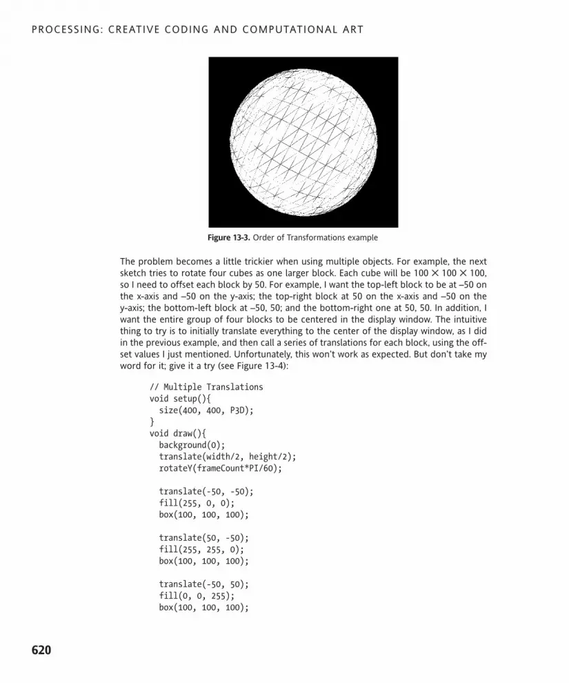
Figure 13-3. Order of Transformations example
The problem becomes a little trickier when using multiple objects. For example, the nextsketch tries to rotate four cubes as one larger block. Each cube will be 100 ! 100 ! 100,so I need to offset each block by 50. For example, I want the top-left block to be at –50 onthe x-axis and –50 on the y-axis; the top-right block at 50 on the x-axis and –50 on the y-axis; the bottom-left block at –50, 50; and the bottom-right one at 50, 50. In addition, Iwant the entire group of four blocks to be centered in the display window. The intuitivething to try is to initially translate everything to the center of the display window, as I didin the previous example, and then call a series of translations for each block, using the off-set values I just mentioned. Unfortunately, this won’t work as expected. But don’t take myword for it; give it a try (see Figure 13-4):
// Multiple Translationsvoid setup(){size(400, 400, P3D);
}void draw(){background(0);translate(width/2, height/2);rotateY(frameCount*PI/60);
translate(-50, -50);fill(255, 0, 0);box(100, 100, 100);
translate(50, -50);fill(255, 255, 0);box(100, 100, 100);
translate(-50, 50);fill(0, 0, 255);box(100, 100, 100);
PROCESSING: CREATIVE CODING AND COMPUTATIONAL ART
620
617xCH13.qxd 4/18/07 3:24 PM Page 620

translate(50, 50);fill(0, 255, 0);box(100, 100, 100);
}
Figure 13-4. Multiple Translations example
So what happened? Translations are cumulative. Each time you call translate(), theentire drawing context of the display window is translated. For example, here’s a series oftranslations that move a box across the screen (see Figure 13-5):
void setup(){size(400, 100, P3D);
}void draw(){background(255);translate(10, height/2);for (int i=10; i<width-20; i+=10){translate(10, 0);box(10, 10, 10);
}}
Figure 13-5. Cumulative Translations example
You’ll notice that I called translate() twice. The first call happens within draw(), whilethe second call is inside the for loop within draw(). When a transformation such as atranslation happens within draw(), it is reset each time that draw() executes. Thus, not tocontradict myself from the earlier paragraph, but the first call, translate(10, height/2),is actually not cumulative. However, the second call, translate(10, 0); within the forloop, executes 37 times each time draw() runs, which creates the cumulative translations
3D
621
13
617xCH13.qxd 4/18/07 3:24 PM Page 621

as the block is offset across the stage. Returning to the rotating block wall, how would yousolve this problem?
Processing comes equipped with two handy functions to solve the problem: pushMatrix()and popMatrix(). These functions work in pairs and allow you to temporarily offset thedrawing context of the display window, draw something, and then put the drawing contextback to where it was before you transformed it. Pretty cool, right? Here’s the fixed rotat-ing wall utilizing the two functions (see Figure 13-6):
// Multiple Translations with pushMatrix() and popMatrix()void setup(){size(400, 400, P3D);
}void draw(){background(0);translate(width/2, height/2);rotateY(frameCount*PI/60);
pushMatrix();translate(-50, -50);fill(255, 0, 0);box(100, 100, 100);popMatrix();
pushMatrix();translate(50, -50);fill(255, 255, 0);box(100, 100, 100);popMatrix();
pushMatrix();translate(50, 50);fill(0, 0, 255);box(100, 100, 100);popMatrix();
pushMatrix();translate(-50, 50);fill(0, 255, 0);box(100, 100, 100);popMatrix();
}
PROCESSING: CREATIVE CODING AND COMPUTATIONAL ART
622
617xCH13.qxd 4/18/07 3:24 PM Page 622

Figure 13-6. Multiple Translations with pushMatrix() and popMatrix() example
Notice how the pushMatrix() and popMatrix() functions surround the translate() andbox() calls. pushMatrix() must come before popMatrix(), and they need to work as apair. The underlying math and theory behind these functions is not simple, but using themreally is. You can even nest these function calls, as long as you have a popMatrix() foreach pushMatrix(). The next example, shown in Figure 13-7, constructs a cube of cubes.The fill color is controlled by the counters in the three for loops. I also made the colortranslucent, in order to reveal the multicube structure.
// Cubic Gridfloat boxSize = 40;float margin = boxSize*2;float depth = 400;color boxFill;
void setup(){size(400, 400, P3D);noStroke();
}
void draw(){background(255);// center and spin gridtranslate(width/2, height/2, -depth/2);rotateY(frameCount*PI/60);rotateX(frameCount*PI/60);
// build grid using multiple translationsfor (float i=-depth/2+margin; i<=depth/2-margin; i+=boxSize){pushMatrix();for (float j=-height/2+margin; j<=height/2-margin; j+=boxSize){pushMatrix();
3D
623
13
617xCH13.qxd 4/18/07 3:24 PM Page 623

for (float k=-width/2+margin; k<=width/2-margin; k+=boxSize){// base fill color on counter values, abs function// ensures values stay within legal rangeboxFill = color(abs(i), abs(j), abs(k), 50);pushMatrix();translate(k, j, i);fill(boxFill);box(boxSize, boxSize, boxSize);popMatrix();
}popMatrix();
}popMatrix();
}}
Figure 13-7. Cubic Grid sketch
So 3D seems pretty easy, right? Well, as you no doubt suspect, there is a lot of stuff goingon beneath Processing’s surface when it come to 3D—stuff that looks truly scary (even tofolks who enjoy math). Not to pop your happy bubble, but I’d like to take just a little lookunder the hood (but well above the really nasty stuff). Since I’ve been using Processing’sbox() function, I’ll show you how to create a custom version of the command, as well assome custom rotation methods. I think seeing how a cube is constructed will give you abetter sense about how to think in 3D. I also think it will begin to give you insight into howto create other 3D geometry besides Processing’s box and sphere. You’ll continue to useProcessing’s translate() function to center your geometry; so you’ll design your cube tobe centered at the origin, which, if you’ll remember, is (0, 0, 0) in 3D. You’ll also build thecube using object-oriented methodology, with classes. Finally, you’ll give your cube anextra feature or two beyond Processing’s built-in version.
PROCESSING: CREATIVE CODING AND COMPUTATIONAL ART
624
617xCH13.qxd 4/18/07 3:24 PM Page 624

Creating a custom cubeTo begin to think about a cube, you need to think about the components of a cube. Acube can be thought of in a number of ways: as a group of points defining the cube’s ver-tices, sometimes referred to as a point cloud; as a wireframe, representing the lines con-necting the cube’s vertices; or as a solid, composed of polygonal sides or faces. In a moreadvanced example, you might also look at different shading and surface material algo-rithms to create a photorealistically textured cube. This section will begin with the creationof a simple class that holds the three x, y, and z coordinates for each of the cube’s vertices.The class will be named Point3D.
/*Extremely simple class tohold each 3D vertex*/class Point3D{float x, y, z;
// constructorsPoint3D(){}
Point3D(float x, float y, float z){this.x = x;this.y = y;this.z = z;
}}
I hope this class looks self-explanatory. I’m using the class simply to group the three com-ponent properties of each vertex. As a refresher, to create a Point3D object and then out-put its component properties, you’d write the following:
void setup(){Point3D p1 = new Point3D(-50, -50, -50);println(p1.x + ", " + p1.y + ", " + p1.z);
}
/*Extremely simple class tohold each 3D vertex*/class Point3D{
float x, y, z;
// constructorsPoint3D(){}
3D
625
13
617xCH13.qxd 4/18/07 3:24 PM Page 625

Point3D(float x, float y, float z){this.x = x;this.y = y;this.z = z;
}}
If you run this, you should see the following output: -50.0, -50.0, -50.0.
Next, you’ll create your Cube class.
I should point out that technically a cube would be composed only of equal-area squarefaces. However, my Cube class will allow you to specify different values for width, height,and depth; sorry if this offends any of you purists out there.
The Cube class will rely on the Point3D class in a compostional relationship, in which I’llembed variables of type Point3D directly within the Cube class. Remember, each cube willbe created around the origin, so I won’t account for an x, y, or z property for the entirecube; only the cube’s overall width, height, and depth properties will be specified, similarlyto how Processing’s box() function works. (The class code that follows will not execute onits own, but you probably realize that by now.)
class Cube{Point3D[] vertices = new Point3D[24];float w, h, d;
// constructors// default constructorCube(){}
Cube(float w, float h, float d){this.w = w;this.h = h;this.d = d;
// cube composed of 6 quads//frontvertices[0] = new Point3D(-w/2,-h/2,d/2);vertices[1] = new Point3D(w/2,-h/2,d/2);vertices[2] = new Point3D(w/2,h/2,d/2);vertices[3] = new Point3D(-w/2,h/2,d/2);//leftvertices[4] = new Point3D(-w/2,-h/2,d/2);vertices[5] = new Point3D(-w/2,-h/2,-d/2);vertices[6] = new Point3D(-w/2,h/2,-d/2);vertices[7] = new Point3D(-w/2,h/2,d/2);//right
PROCESSING: CREATIVE CODING AND COMPUTATIONAL ART
626
617xCH13.qxd 4/18/07 3:24 PM Page 626
vertices[8] = new Point3D(w/2,-h/2,d/2);vertices[9] = new Point3D(w/2,-h/2,-d/2);vertices[10] = new Point3D(w/2,h/2,-d/2);vertices[11] = new Point3D(w/2,h/2,d/2);//backvertices[12] = new Point3D(-w/2,-h/2,-d/2);vertices[13] = new Point3D(w/2,-h/2,-d/2);vertices[14] = new Point3D(w/2,h/2,-d/2);vertices[15] = new Point3D(-w/2,h/2,-d/2);//topvertices[16] = new Point3D(-w/2,-h/2,d/2);vertices[17] = new Point3D(-w/2,-h/2,-d/2);vertices[18] = new Point3D(w/2,-h/2,-d/2);vertices[19] = new Point3D(w/2,-h/2,d/2);//bottomvertices[20] = new Point3D(-w/2,h/2,d/2);vertices[21] = new Point3D(-w/2,h/2,-d/2);vertices[22] = new Point3D(w/2,h/2,-d/2);vertices[23] = new Point3D(w/2,h/2,d/2);
}
void create(){// draw cubefor (int i=0; i<6; i++){beginShape(QUADS);for (int j=0; j<4; j++){vertex(vertices[j+4*i].x, vertices[j+4*i].y, "
vertices[j+4*i].z);}endShape();
}}
}
The Cube class is divided into two constructors and a create() method. The first con-structor is just the default no-arguments constructor, in case a Cube object is instantiatedwithout any initial values. The second constructor takes three arguments and assemblesthe data, while the create() method actually handles the drawing. In comparison to theCube class, Processing’s box() function, which seems to handle both instantiation anddrawing, might initially seem like a better procedural model—it’s certainly less work.However, suppose you wanted to pass Cube objects to another class that would then takecare of positioning and drawing the cubes—you’d need to separate the object creationfrom the actual drawing of the object, as in the preceding example. The second construc-tor initializes the vertices array, which holds 24 Point3D objects. Although a cube looks likeit only has eight unique points, it’s simpler (for now) to think of a cube as six separatequadrangle faces composed of four points each. This will prevent you from having to usesome of the points for more than one face (which you’ll eventually learn how to doas well).
3D
627
13
617xCH13.qxd 4/18/07 3:24 PM Page 627

The create() method includes a nested for loop that is a bit dense to untangle. I neededan algorithm that would run through the vertices array and treat each individual face as aself-contained quadrangle (composed of four points). Notice that the beginShape() andendShape() functions are nested within the outer for loop as well, allowing each face tobe drawn as a separate unit. This structure will also allow you to easily customize the colorof each face, which we’ll look at shortly. However, before getting into that, I’ll show youhow to use the two classes just created to generate a cube.
Here’s some runnable code. (Please note that I didn’t repeat the code from the Point3Dand Cube classes shown previously. Just make sure you add the two classes beneath the fol-lowing code, or put each class in its own tab.)
Cube c1;void setup(){size(400, 400, P3D);c1 = new Cube(200, 200, 200);c1.create();
}// Don't forget to add the Point3D and Cube classes code
I also want to translate the cube to the middle of the drawing space, or at least haveit move around some. I’ll use Processing’s translate() and rotate() functions inconjunction with the classes to achieve this. In addition, I’ll create an overloadedcreate(color[]quadBG) method for customizing the color of each quad face.
The next example, shown in Figure 13-8, creates two cubes, using the two overloaded cre-ate() methods. Since I added an additional create() method to the Cube class, I’veincluded the updated class code in the following example. I didn’t repeat the Point3Dclass, which you’ll need as well to run the example; simply paste it below the Cube class orput it into its own tab.
// Two Rotating Custom Cubes
// custom Cube reference variablesCube c1, c2;// array to hold different face colorscolor[]quadBG = new color[6];
void setup(){size(400, 400, P3D);quadBG[0] = color(175, 30, 30, 150);quadBG[1] = color(30, 175, 30, 150);
You may remember that an overloaded method is an object-oriented conceptmeaning that more than one method with the same name exists in a class. Whatdifferentiates the same named methods is the number and type of parametersbetween the parentheses in the head of the method. You can read more aboutoverloaded methods and other object-oriented concepts in Chapter 8.
PROCESSING: CREATIVE CODING AND COMPUTATIONAL ART
628
617xCH13.qxd 4/18/07 3:24 PM Page 628

quadBG[2] = color(30, 30, 175, 150);quadBG[3] = color(175, 175, 30, 150);quadBG[4] = color(175, 30, 175, 150);quadBG[5] = color(175, 87, 30, 150);c1 = new Cube(200, 200, 200);c2 = new Cube(100, 100, 100);
}
void draw(){background(100);translate(width/2, height/2);rotateX(frameCount*PI/50);rotateY(frameCount*PI/60);// create larger colored cubenoStroke();c1.create(quadBG);// create inner black cubefill(0, 200);stroke(255);c2.create();
}
// Updated custom Cube classclass Cube{Point3D[] vertices = new Point3D[24];float w, h, d;
// Constructors// default constructorCube(){}
// constructor 2Cube(float w, float h, float d){this.w = w;this.h = h;this.d = d;
// cube composed of 6 quads//frontvertices[0] = new Point3D(-w/2,-h/2,d/2);vertices[1] = new Point3D(w/2,-h/2,d/2);vertices[2] = new Point3D(w/2,h/2,d/2);vertices[3] = new Point3D(-w/2,h/2,d/2);//leftvertices[4] = new Point3D(-w/2,-h/2,d/2);vertices[5] = new Point3D(-w/2,-h/2,-d/2);vertices[6] = new Point3D(-w/2,h/2,-d/2);vertices[7] = new Point3D(-w/2,h/2,d/2);
3D
629
13
617xCH13.qxd 4/18/07 3:24 PM Page 629

//rightvertices[8] = new Point3D(w/2,-h/2,d/2);vertices[9] = new Point3D(w/2,-h/2,-d/2);vertices[10] = new Point3D(w/2,h/2,-d/2);vertices[11] = new Point3D(w/2,h/2,d/2);//backvertices[12] = new Point3D(-w/2,-h/2,-d/2);vertices[13] = new Point3D(w/2,-h/2,-d/2);vertices[14] = new Point3D(w/2,h/2,-d/2);vertices[15] = new Point3D(-w/2,h/2,-d/2);//topvertices[16] = new Point3D(-w/2,-h/2,d/2);vertices[17] = new Point3D(-w/2,-h/2,-d/2);vertices[18] = new Point3D(w/2,-h/2,-d/2);vertices[19] = new Point3D(w/2,-h/2,d/2);//bottomvertices[20] = new Point3D(-w/2,h/2,d/2);vertices[21] = new Point3D(-w/2,h/2,-d/2);vertices[22] = new Point3D(w/2,h/2,-d/2);vertices[23] = new Point3D(w/2,h/2,d/2);
}void create(){// draw cubefor (int i=0; i<6; i++){beginShape(QUADS);for (int j=0; j<4; j++){vertex(vertices[j+4*i].x, vertices[j+4*i].y, "
vertices[j+4*i].z);}endShape();
}}void create(color[]quadBG){// draw cubefor (int i=0; i<6; i++){fill(quadBG[i]);beginShape(QUADS);for (int j=0; j<4; j++){vertex(vertices[j+4*i].x, vertices[j+4*i].y, "
vertices[j+4*i].z);}endShape();
}}
}// This example requires the Point3D class.
PROCESSING: CREATIVE CODING AND COMPUTATIONAL ART
630
617xCH13.qxd 4/18/07 3:24 PM Page 630
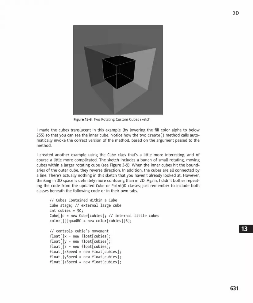
Figure 13-8. Two Rotating Custom Cubes sketch
I made the cubes translucent in this example (by lowering the fill color alpha to below255) so that you can see the inner cube. Notice how the two create() method calls auto-matically invoke the correct version of the method, based on the argument passed to themethod.
I created another example using the Cube class that’s a little more interesting, and ofcourse a little more complicated. The sketch includes a bunch of small rotating, movingcubes within a larger rotating cube (see Figure 3-9). When the inner cubes hit the bound-aries of the outer cube, they reverse direction. In addition, the cubes are all connected bya line. There’s actually nothing in this sketch that you haven’t already looked at. However,thinking in 3D space is definitely more confusing than in 2D. Again, I didn’t bother repeat-ing the code from the updated Cube or Point3D classes; just remember to include bothclasses beneath the following code or in their own tabs.
// Cubes Contained Within a CubeCube stage; // external large cubeint cubies = 50;Cube[]c = new Cube[cubies]; // internal little cubescolor[][]quadBG = new color[cubies][6];
// controls cubie's movementfloat[]x = new float[cubies];float[]y = new float[cubies];float[]z = new float[cubies];float[]xSpeed = new float[cubies];float[]ySpeed = new float[cubies];float[]zSpeed = new float[cubies];
3D
631
13
617xCH13.qxd 4/18/07 3:24 PM Page 631

// controls cubie's rotationfloat[]xRot = new float[cubies];float[]yRot = new float[cubies];float[]zRot = new float[cubies];
// size of external cubefloat bounds = 300;
void setup(){size(400, 400, P3D);for (int i=0; i<cubies; i++){// each cube face has a random color componentfloat colorShift = random(-75, 75);quadBG[i][0] = color(175+colorShift, 30, 30);quadBG[i][1] = color(30, 175+colorShift, 30);quadBG[i][2] = color(30, 30, 175+colorShift);quadBG[i][3] = color(175+colorShift, 175+colorShift, 30);quadBG[i][4] = color(175+colorShift, 30, 175+colorShift);quadBG[i][5] = color(175+colorShift, 87+colorShift, 30);
// cubies are randomly sizedfloat cubieSize = random(5, 15);c[i] = new Cube(cubieSize, cubieSize, cubieSize);
//initialize cubie's position, speed and rotationx[i] = 0;y[i] = 0;z[i] = 0;
xSpeed[i] = random(-2, 2);ySpeed[i] = random(-2, 2);zSpeed[i] = random(-2, 2);
xRot[i] = random(40, 100);yRot[i] = random(40, 100);zRot[i] = random(40, 100);
}// instantiate external large cubestage = new Cube(300, 300, 300);
}
void draw(){background(50);// center in display windowtranslate(width/2, height/2, -130);
PROCESSING: CREATIVE CODING AND COMPUTATIONAL ART
632
617xCH13.qxd 4/18/07 3:24 PM Page 632
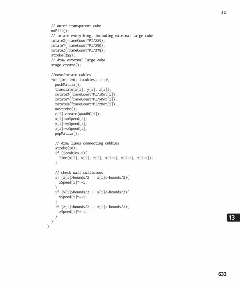
// outer transparent cubenoFill();// rotate everything, including external large cuberotateX(frameCount*PI/225);rotateY(frameCount*PI/250);rotateZ(frameCount*PI/275);stroke(255);// draw external large cubestage.create();
//move/rotate cubiesfor (int i=0; i<cubies; i++){pushMatrix();translate(x[i], y[i], z[i]);rotateX(frameCount*PI/xRot[i]);rotateY(frameCount*PI/yRot[i]);rotateX(frameCount*PI/zRot[i]);noStroke();c[i].create(quadBG[i]);x[i]+=xSpeed[i];y[i]+=ySpeed[i];z[i]+=zSpeed[i];popMatrix();
// draw lines connecting cubbiesstroke(10);if (i<cubies-1){line(x[i], y[i], z[i], x[i+1], y[i+1], z[i+1]);
}
// check wall collisionsif (x[i]>bounds/2 || x[i]<-bounds/2){xSpeed[i]*=-1;
}if (y[i]>bounds/2 || y[i]<-bounds/2){ySpeed[i]*=-1;
}if (z[i]>bounds/2 || z[i]<-bounds/2){zSpeed[i]*=-1;
}}
}
3D
633
13
617xCH13.qxd 4/18/07 3:24 PM Page 633

Figure 13-9. Cubes Contained Within a Cube sketch
This example is long—but again, it’s stuff you’ve looked at before. The most complex partof the sketch is the following code snippet, within the for loop of the draw() function:
pushMatrix();translate(x[i], y[i], z[i]);rotateX(frameCount*PI/xRot[i]);rotateY(frameCount*PI/yRot[i]);rotateX(frameCount*PI/zRot[i]);noStroke();c[i].create(quadBG[i]);x[i]+=xSpeed[i];y[i]+=ySpeed[i];z[i]+=zSpeed[i];popMatrix();
It is sometimes confusing, when using the pushMatrix() and popMatrix() functions, todetermine what commands need to be called between them. Since I’m using a loop toprocess an array of items, I need to make sure that each transformation only affects itsrespective item; otherwise, the transformations will become cumulative, so objects storedlater in the array will be affected much more than the earlier ones. It is helpful to breakdown the last example by commenting out the pushMatrix() and popMatrix() calls andthen rerunning the sketch to see the effect. In addition, I recommend playing with someof the values in the sketch, especially the variables in the following code:
int cubies = 50;float bounds = 300;float cubieSize = random(5, 15);xSpeed[i] = random(-2, 2);ySpeed[i] = random(-2, 2);zSpeed[i] = random(-2, 2);
PROCESSING: CREATIVE CODING AND COMPUTATIONAL ART
634
617xCH13.qxd 4/18/07 3:24 PM Page 634

As complicated as this last sketch might have seemed, it only scratches the surface ofwhat’s possible. For example, a more advanced version of the sketch could include physicscalculations: gravity, collisions, angular or rotational velocities, and so on. Well, don’tworry, I won’t torture you further with this example. However, before moving on, there isone more fundamental concept used in the last example that I’d like to discuss: 3Drotations.
3D rotationsThus far in the chapter, I’ve been happily using Processing’s 3D rotation functions:rotateX(), rotateY(), and rotateZ(). These are really easy to use, which is a goodthing—but it’s also valuable to understand how these functions operate beneath the hood.I actually already covered the basic math that controls 3D rotation when I discussed 2Drotation around the z-axis. In 2D, when you want to rotate around the origin, you use thefollowing trig functions:
y = sin(theta)*radiusx = cos(theta)*radius
Hopefully, these expressions seem like old friends by now (if so, you’re well on your way togeek certification). In 3D, the situation isn’t much more complicated than applying thesesame rotation expressions to the x- and y-axes. To perform rotations around each of thethree individual axes, you’d use the following expressions:
z-axis rotationx = cos(theta)*radiusy = sin(theta)*radius
x-axis rotationy = cos(theta)*radiusz = sin(theta)*radius
y-axis rotationz = cos(theta)*radiusx = sin(theta)*radius
These expressions work fine for single-axis rotations, but if you want to put a bunch ofthese together, or allow a user to randomly rotate a shape around any axis in real time,you need slightly more complicated versions of these equations. Before looking at those,here’s a simple implementation that rotates three rectangles around the x-, y-, and z-axes(see Figure 13-10):
// Single Axis 3D Rotation
// rectangle verticesfloat[][]rectX = new float[3][4];float[][]rectY = new float[3][4];float[][]rectZ = new float[3][4];
3D
635
13
617xCH13.qxd 4/18/07 3:24 PM Page 635

// rotation variablesfloat[]angle = {45, 45, 45};float[]rot = {1, 1, 1};
void setup(){size (400, 200, P3D);
}
void draw(){background(255);for (int i=0; i<3; i++){pushMatrix();// spread rects evenly across windowtranslate(75+(125*i), height/2);beginShape();for (int j=0; j<4; j++){// rotation around z-axisif (i==0){rectX[i][j] = cos(radians(angle[i]))*50;rectY[i][j] = sin(radians(angle[i]))*50;
}// rotation around x-axiselse if (i==1){rectY[i][j] = cos(radians(angle[i]))*50;rectZ[i][j] = sin(radians(angle[i]))*50;
// offset added just to show rotation betterrectX[i][j] = 10;
}// rotation around y-axiselse if (i==2){rectZ[i][j] = cos(radians(angle[i]))*50;rectX[i][j] = sin(radians(angle[i]))*50;
// offset added just to show rotation betterrectY[i][j] = 10;
}vertex(rectX[i][j], rectY[i][j], rectZ[i][j]);angle[i]+=360/4;angle[i]+=rot[i];
}endShape(CLOSE);popMatrix();
}}
PROCESSING: CREATIVE CODING AND COMPUTATIONAL ART
636
617xCH13.qxd 4/18/07 3:24 PM Page 636
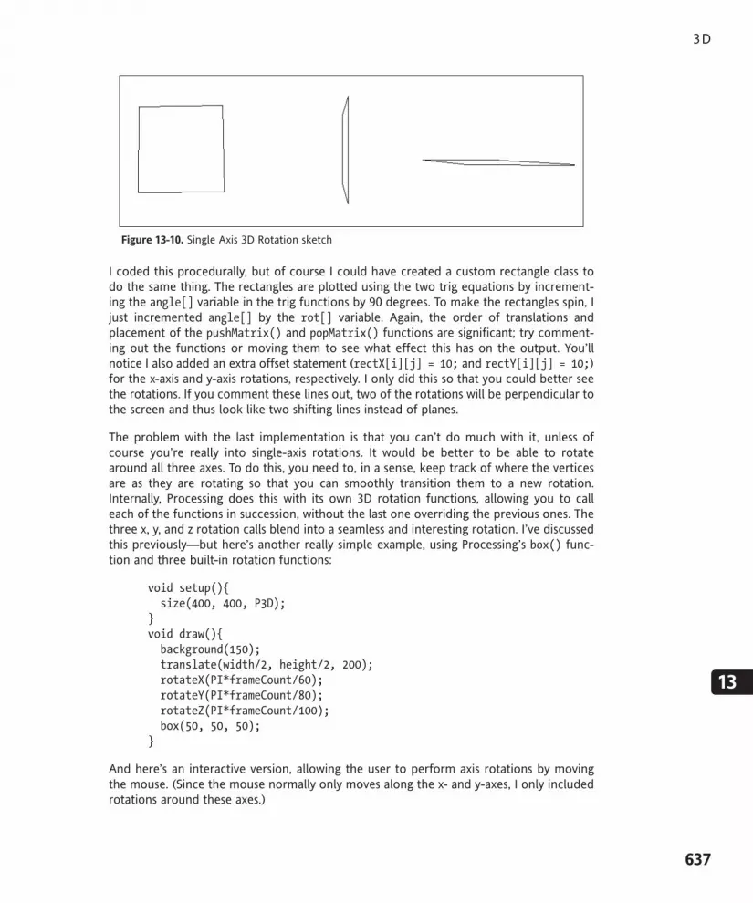
Figure 13-10. Single Axis 3D Rotation sketch
I coded this procedurally, but of course I could have created a custom rectangle class todo the same thing. The rectangles are plotted using the two trig equations by increment-ing the angle[] variable in the trig functions by 90 degrees. To make the rectangles spin, Ijust incremented angle[] by the rot[] variable. Again, the order of translations andplacement of the pushMatrix() and popMatrix() functions are significant; try comment-ing out the functions or moving them to see what effect this has on the output. You’llnotice I also added an extra offset statement (rectX[i][j] = 10; and rectY[i][j] = 10;)for the x-axis and y-axis rotations, respectively. I only did this so that you could better seethe rotations. If you comment these lines out, two of the rotations will be perpendicular tothe screen and thus look like two shifting lines instead of planes.
The problem with the last implementation is that you can’t do much with it, unless ofcourse you’re really into single-axis rotations. It would be better to be able to rotatearound all three axes. To do this, you need to, in a sense, keep track of where the verticesare as they are rotating so that you can smoothly transition them to a new rotation.Internally, Processing does this with its own 3D rotation functions, allowing you to calleach of the functions in succession, without the last one overriding the previous ones. Thethree x, y, and z rotation calls blend into a seamless and interesting rotation. I’ve discussedthis previously—but here’s another really simple example, using Processing’s box() func-tion and three built-in rotation functions:
void setup(){size(400, 400, P3D);
}void draw(){background(150);translate(width/2, height/2, 200);rotateX(PI*frameCount/60);rotateY(PI*frameCount/80);rotateZ(PI*frameCount/100);box(50, 50, 50);
}
And here’s an interactive version, allowing the user to perform axis rotations by movingthe mouse. (Since the mouse normally only moves along the x- and y-axes, I only includedrotations around these axes.)
3D
637
13
617xCH13.qxd 4/18/07 3:24 PM Page 637

float rotX, rotY;void setup(){size(400, 400, P3D);
}void draw(){background(150);translate(width/2, height/2, 200);rotateX(rotX);rotateY(rotY);box(50, 50, 50);
}void mouseMoved(){rotX = radians(mouseY);rotY = radians(mouseX);
}
So that was the easy way. Of course, you by now know that I can’t leave well enough alone.Next, I’ll show you how to re-create the functionality of Processing’s three rotation func-tions, which mostly just means altering the trig functions. Here they are, along with somedeclared variables to help illustrate how they work. (Please note that this code is notmeant to be run.)
float originalX, originalY, originalZ;float x2, y2, z2;float x3, y3, z3;float finalX, finalY, finalZ;
// rotation around x-axixy2 = cos(angleX) * originalY - sin(angleX) * originalZ;z2 = sin(angleX) * originalY + cos(angleX) * originalZ;
// rotation around y-axisz3 = cos(angleY) * z2 - sin(angleY) * x2;x3 = sin(angleY) * z2 + cos(angleY) * x2;
// rotation around z-axisfinalX = cos(angleZ) * x3 - sin(angleZ) * y3;finalY = sin(angleZ) * x3 + cos(angleZ) * y3;
Although the expressions may at first seem a little confusing, if you look at them carefully,you’ll see that they’re pretty redundant. A key feature to using these expressions, whichsome books don’t seem to clarify properly, is that the expressions use existing x, y, and zvalues as inputs. So, for example, if you wanted to do rotations around all three axes,you’d need to keep feeding the new values calculated from the previous axis rotations intothe next set of expressions, as I illustrated by using the different variables. I accomplish thisin the next example by using three separate vertices arrays in addition to the original arrayof vertices; it’s mostly an organizational problem.
PROCESSING: CREATIVE CODING AND COMPUTATIONAL ART
638
617xCH13.qxd 4/18/07 3:24 PM Page 638

The first example I’ll look at simply rotates a rectangle, which is coded procedurally. In thesecond example, I’ll reuse the Cube and Point3D classes to rotate a cube. Here’s the codefor the first example (shown in Figure 13-11):
// Custom Rotation of a Rectangle Around the X-, Y-, and Z-Axes
// rectangle's vertices before rotationfloat[][]originalVertices = new float[4][3];
// rectangle's vertices after rotationfloat[][]transformedVertices = new float[4][3];
// control rectangle rotationsfloat angleX, angleY, angleZ;
void setup(){size(400, 400, P3D);
/* generate initial rectangle coordinate datafilling originalVertices array */
// creates rectangle parallel to windowfloat angle = 45;for (int i=0; i<4; i++){originalVertices[i][0] = cos(radians(angle))*50;originalVertices[i][1] = sin(radians(angle))*50;originalVertices[i][2] = 0;angle+=360/4.0;
}}
void draw(){background(100);// rotate rectangle around all 3 axesmyRotateX(2);myRotateY(6);myRotateZ(3);
//draw rectcreateRect();
}
void myRotateX(float deg){angleX+=deg;
}void myRotateY(float deg){angleY+=deg;
}void myRotateZ(float deg){angleZ+=deg;
}
3D
639
13
617xCH13.qxd 4/18/07 3:24 PM Page 639

void createRect(){translate(width/2, height/2, 200);transformedVertices = rotateVertices();beginShape();for (int i=0; i<4; i++){vertex(transformedVertices[i][0], transformedVertices[i][1], "
transformedVertices[i][2]);}endShape(CLOSE);
}
// called every framefloat[][]rotateVertices(){
// arrays to temporarily store rotated verticesfloat[][]rotatedVertices_XAxis = new float[4][3];float[][]rotatedVertices_YAxis = new float[4][3];float[][]rotatedVertices_ZAxis = new float[4][3];
for (int i=0; i<4; i++){// rotation around x-axisrotatedVertices_XAxis[i][0] = originalVertices[i][0];rotatedVertices_XAxis[i][1] = cos(radians(angleX))* "
originalVertices[i][1] - sin(radians(angleX))* "originalVertices[i][2];
rotatedVertices_XAxis[i][2] = sin(radians(angleX))* "originalVertices[i][1] + cos(radians(angleX))* "originalVertices[i][2];
// rotation around y-axisrotatedVertices_YAxis[i][1] = rotatedVertices_XAxis[i][1];rotatedVertices_YAxis[i][2] = cos(radians(angleY))* "
rotatedVertices_XAxis[i][2] - sin(radians(angleY))* "rotatedVertices_XAxis[i][0];
rotatedVertices_YAxis[i][0] = sin(radians(angleY))* "rotatedVertices_XAxis[i][2] + cos(radians(angleY))* "rotatedVertices_XAxis[i][0];
// rotation around z-axisrotatedVertices_ZAxis[i][0] = cos(radians(angleZ))* "
rotatedVertices_YAxis[i][0] - sin(radians(angleZ))* "rotatedVertices_YAxis[i][1];
rotatedVertices_ZAxis[i][1] = sin(radians(angleZ))* "rotatedVertices_YAxis[i][0] + cos(radians(angleZ))* "rotatedVertices_YAxis[i][1];
rotatedVertices_ZAxis[i][2] = rotatedVertices_YAxis[i][2];}return rotatedVertices_ZAxis;
}
PROCESSING: CREATIVE CODING AND COMPUTATIONAL ART
640
617xCH13.qxd 4/18/07 3:24 PM Page 640

Figure 13-11. Custom Rotation of a Rectangle Around the X-, Y-, and Z-Axes example
The 2D array float[][]originalVertices is used to store the original rectangle verticesdata, and float[][]transformedVertices is used eventually to receive the transformedvertices data, which is then passed to Processing’s vertex() function for drawing. In thesetup() function, I create the original rectangle with the standard sin() and cos() func-tion approach described in numerous sections of the book. I don’t draw the rectanglehere, but rather construct it in data and assign that data to the originalVertices[][]array. Next, in draw(), I call some custom rotate functions that update the values of theangleX, angleY, and angleZ variables used in the rotation calculations. Finally, I call thecreateRect() function, which internally calls the rotateVertices() function and drawsthe rectangle on the screen. It is in the rotateVertices() function that most of thesketch’s real heavy lifting occurs.
At the top of the rotateVertices() function I declare three 2D arrays. These arrays areused to temporarily store the transformed vertices data. To make things simpler (hon-estly), I set up the sketch to call the rotateVertices() function every time draw()executes. This isn’t the most efficient approach, but it avoids things like having to checkwhich rotation function commands were invoked; I just assume they’re all being called.However, if you comment out any/all of the following lines:
myRotateX(2);myRotateY(6);myRotateZ(3);
the program will still work properly. The rotateVertices() function will still be calledfrom within createRect(), but some/all of the rotation angle values won’t change, soyou’ll get less or no rotation. Reading though the rotateVertices() function should bestraightforward, even though it’s kind of dense. The important thing to notice is how theprevious array’s values are input into the next set of expressions, and how these expres-sions are assigned to one of the temporary arrays. I chose to have the function return thefinal array, which is why I used the expression transformedVertices = rotateVertices();in the createRect() function and created the three temporary arrays (rotatedVertices_XAxis[][], rotatedVertices_YAxis[][], and rotatedVertices_ZAxis[][]) locally within
3D
641
13
617xCH13.qxd 4/18/07 3:24 PM Page 641

the rotateVertices() function; there are certainly other ways to implement this. Beforeyou move on to the cube example, I strongly recommend you play/experiment with thisone for a while.
I’ll reuse the Point3D and Cube classes to build the next example. I’ll need to createanother method to handle the combined 3D rotations. I could redesign the Cube class andadd the new rotation method directly in there. But a much better a way to deal withadding the new method is to create a new class as a subclass of the Cube class. Thisapproach gives me the benefit of using the original class without having to alter it, stillallowing me to extend its capabilities. As discussed earlier in the book, the term inheri-tance in OOP is used to describe this extending approach. Although I could have gone intomy original Cube class and added a rotation method, it’s best practice to not edit existingclasses, as other dependent classes could be adversely affected. The following code givesthe completed example (shown in Figure 13-12). I didn’t include the Point3D or Cube classcode, just the new SpinnyCube class (Cube subclass); so don’t forget to add the Point3Dand Cube classes before running the example. (Remember, you can either create a new tabfor each class, or simply paste the classes beneath your current sketch code.)
// Rotation of a Custom Cube Around the X-, Y-, and Z-Axes
// custom Cube reference variableSpinnyCube c1;
// array to hold different face colorscolor[]quadBG = new color[6];
void setup(){size(400, 400, P3D);quadBG[0] = color(175, 30, 30, 255);quadBG[1] = color(30, 175, 30, 255);quadBG[2] = color(30, 30, 175, 255);quadBG[3] = color(175, 175, 30, 255);quadBG[4] = color(175, 30, 175, 255);quadBG[5] = color(175, 87, 30, 255);
//instantiate cubec1 = new SpinnyCube(200, 200, 200);
}
void draw(){background(100);translate(width/2, height/2);
if (mousePressed){//interactive rotationc1.spinnyRotateX(mouseY);c1.spinnyRotateY(mouseX);
}else {
PROCESSING: CREATIVE CODING AND COMPUTATIONAL ART
642
617xCH13.qxd 4/18/07 3:24 PM Page 642

//automatic rotationc1.spinnyRotateX(frameCount*PI);c1.spinnyRotateY(frameCount*PI/4);c1.spinnyRotateZ(frameCount*PI/5);
}
//draw cubenoStroke();c1.create(quadBG);
}
// SpinnyCube classclass SpinnyCube extends Cube{float angleX, angleY, angleZ;Point3D[] transformedVertices = new Point3D[24];
// default constructorSpinnyCube(){}
// constructorSpinnyCube(float w, float h, float d){// call superclass constructorsuper(w, h, d);
}
// rotation methodvoid spinnyRotateXYZ(){// temporary vertices arraysPoint3D[] rotatedVertices_XAxis = new Point3D[24];Point3D[] rotatedVertices_YAxis = new Point3D[24];Point3D[] rotatedVertices_ZAxis = new Point3D[24];
for (int i=0; i<24; i++){// initialize temp vertices arraysrotatedVertices_XAxis[i] = new Point3D();rotatedVertices_YAxis[i] = new Point3D();rotatedVertices_ZAxis[i] = new Point3D();
// rotation around x-axisrotatedVertices_XAxis[i].x = vertices[i].x;rotatedVertices_XAxis[i].y = cos(radians(angleX))* "
vertices[i].y - sin(radians(angleX))*vertices[i].z;rotatedVertices_XAxis[i].z = sin(radians(angleX))* "
vertices[i].y + cos(radians(angleX))*vertices[i].z;
// rotation around y-axisrotatedVertices_YAxis[i].y = rotatedVertices_XAxis[i].y;rotatedVertices_YAxis[i].z = cos(radians(angleY))* "
3D
643
13
617xCH13.qxd 4/18/07 3:24 PM Page 643

rotatedVertices_XAxis[i].z - sin(radians(angleY))* "rotatedVertices_XAxis[i].x;
rotatedVertices_YAxis[i].x = sin(radians(angleY))* "rotatedVertices_XAxis[i].z + cos(radians(angleY))* "rotatedVertices_XAxis[i].x;
// rotation around z-axisrotatedVertices_ZAxis[i].x = cos(radians(angleZ))* "
rotatedVertices_YAxis[i].x - sin(radians(angleZ))* "rotatedVertices_YAxis[i].y;
rotatedVertices_ZAxis[i].y = sin(radians(angleZ))* "rotatedVertices_YAxis[i].x + cos(radians(angleZ))* "rotatedVertices_YAxis[i].y;
rotatedVertices_ZAxis[i].z = rotatedVertices_YAxis[i].z;}// update transformedVertices arraystransformedVertices = rotatedVertices_ZAxis;
}
// assign rotation angles for each axisvoid spinnyRotateX(float angle){angleX = angle;
}void spinnyRotateY(float angle){angleY = angle;
}void spinnyRotateZ(float angle){angleZ = angle;
}
/* SpinnyCube (subclass) create() methods willoverride Cube (superclass) create() methods. */
void create(){// draw cubespinnyRotateXYZ();stroke(0);for (int i=0; i<6; i++){beginShape(QUADS);for (int j=0; j<4; j++){vertex(transformedVertices[j+4*i].x, transformedVertices[j+ "
4*i].y, transformedVertices[j+4*i].z);}endShape();
}}void create(color[]quadBG){// draw cubespinnyRotateXYZ();
PROCESSING: CREATIVE CODING AND COMPUTATIONAL ART
644
617xCH13.qxd 4/18/07 3:24 PM Page 644

for (int i=0; i<6; i++){fill(quadBG[i]);beginShape(QUADS);for (int j=0; j<4; j++){vertex(transformedVertices[j+4*i].x, transformedVertices[j+ "
4*i].y, transformedVertices[j+4*i].z);}endShape();
}}
}
Figure 13-12. Rotation of a Custom Cube Around the X-, Y-, and Z-Axes example
The example begins similarly to the earlier cube example, except that I’m using my newSpinnyCube reference type to declare variable c1. Remember, a class is a legal data type,just as float, int, and color are. Since the SpinnyCube class extends the Cube class, I wasable to instantiate the SpinnyCube object with the help of the constructor in the Cubesuperclass. If this doesn’t make sense yet, it will become clearer shortly (and you canalways refer back to Chapter 8 for a review on OOP).
Within the draw() function, I set up a simple if...else block that starts the cube spinningand allows the user to drag and rotate the cube. The last line in draw() is the create()method that handles drawing the cube. Below the draw() function is the SpinnyCube class.
Even though I used an OOP approach for this example, the SpinnyCube class is imple-mented quite similarly to the last procedural spinning rectangle example. I declared atransformedVertices[] array to eventually handle the rotated vertices. The drawing codeuses this array. I didn’t need to create the original vertices[] array, as I have access to allthe members (properties and methods) in the Cube class (through inheritance), which
3D
645
13
617xCH13.qxd 4/18/07 3:24 PM Page 645

contains this array. The SpinnyCube constructor accepts the same three arguments as theCube class, for the width, height, and depth of the cube. The first line of the SpinnyCubeconstructor
super(w, h, d);
passes the arguments through to the superclass (Cube) constructor. This is a very efficientstructure that allows you to build upon base and component classes. One little reminder—if there had been any other code in the SpinnyCube constructor, it would need to be putafter the super() call, which (when included) must always be the first line in the subclassconstructor. (However, you are not required to include a call to super() in a subclass con-structor.)
Following the constructors is the spinnyRotateXYZ() method. This method works practi-cally identically to the rotateVertices() function in the previous example. To keep thingsorganized, I declared and initialized all the temporary vertices arrays locally within thismethod. As in the last example, the transformed vertices need to be plugged into the nextset of expressions. Finally, at the end of the method, I assigned the updated vertices to thetransformedVertices[] array used to draw the cube. Following this method are threesimple utility methods (spinnyRotateX(), spinnyRotateY(), and spinnyRotateZ()) thatupdate rotation angles, used by the expressions in the spinnyRotateXYZ() method.
The last methods in the SpinnyCube class are two overloaded create() methods, just as inthe Cube class. Creating two more methods with the same name may seem confusing andunnecessary, since the subclass has access to the superclass’s create() methods. I wantedto call the spinnyRotate() method internally from within the create() methods, and Ididn’t want to make that change to the cube’s original create() methods. Since the cre-ate() methods in the SpinnyCube subclass have the same method signatures (parameterlists) as the create() methods in the Cube superclass, the methods in the subclass willoverride the same named ones in the superclass. In other words, when I call
c1.create(quadBG);
and c1 is of type SpinnyCube, the create() method in the SpinnyCube subclass is exe-cuted, not the one with the identical signature in the Cube class. The SpinnyCube create()methods are implemented nearly identically to the ones in the Cube class, except that theyhave additional lines for calling the spinnyRotateXYZ() method.
I recommend always adding a default no-argument constructor to any class that willbe extended, since the superclass constructor is always invoked, even without anexplicit call to super(). To learn more about this and related (albeit geeky and low-level) issues, check out www.beginner-java-tutorial.com/ and http://java.sun.com/docs/books/jls/second_edition/html/classes.doc.html.
PROCESSING: CREATIVE CODING AND COMPUTATIONAL ART
646
617xCH13.qxd 4/18/07 3:24 PM Page 646

Beyond box() and sphere()While there are many common 3D primitives (including cylinders, pyramids, cones, andtoroids), Processing’s built-in primitive-creation functions are limited to the measly box()and sphere(). I’ll show you how to construct a few of these—which is mostly a matter ofcreating algorithms. What I mean by this is that you need a set of logical instructions tocreate these forms (unless you’re a math genius, which I’m not). Sometimes forms seemcomplex until you see the steps to generate them. Before switching shapes, I’ll develop analgorithm to construct a brick tower (shown in Figure 13-13) that includes a crenellatedroof, using the existing Cube class.
The tower will be constructed of rings of bricks with a rotational offset between the brickrows, allowing the vertically adjacent brick seams to alternate, like in a regular brick wall.The first part of the algorithm generates a single ring of bricks; next, the graphics context(the object that controls the actual drawing) is translated the distance equal to the heightof a brick and rotated one-half the ring rotation angle so that the vertical seams alternate.Then the first step is repeated until some specified height is reached. Finally, the last stepinvolves creating the crenellation, which uses the same basic routine as step 1 (generatinga brick ring), but with every other brick removed (actually never added).
To generate the initial brick ring, I used the following trig expressions:
z = cos(radians(angle))*radius;x = sin(radians(angle))*radius;
These expressions, which were discussed earlier in the chapter, can be used to generate aregular polygon that is flipped to face the top and bottom of the display window. In addi-tion to placing the bricks in a ring in the xz plane, I also need to rotate the bricks so thatthey are aligned with the ring path. I accomplished this by rotating each brick the samenumber of degrees I displaced it to form the ring. To help understand this, imagine thatyou have a brick floating in front of your eyes. The brick’s wide side is facing you, as if youwere looking straight at a building. Now displace the brick 90 degrees around your head(but don’t rotate it), so that it’s next to your left ear. The brick’s end is now facing your ear.To make the wide side of the brick again face your head (actually, your ear), you need torotate the brick around its center point the same number of degrees it was displaced (i.e.,90 degrees).
Following is the code for the example, which requires the Cube and Point3D classes:
// Brick Tower
// Point3D and Cube classes required.float bricksPerLayer = 16.0; // value must be evenfloat brickLayers = 25.0;Cube[]bricks = new Cube[int(bricksPerLayer*brickLayers)];float brickWidth = 60, brickHeight = 25, brickDepth = 25;float radius = 150.0;float angle = 0;
3D
647
13
617xCH13.qxd 4/18/07 3:24 PM Page 647

void setup(){size(400, 400, P3D);
//instantiate bricksfor (int i=0; i<bricks.length; i++){bricks[i] = new Cube(brickWidth, brickHeight, brickDepth);
}}
void draw(){background(100, 125, 200);float tempX = 0, tempY = 0, tempZ = 0;fill(175, 87, 20);stroke(100, 50, 10);// add basic light setuplights();translate(width/2, height*1.2, -550);// tip tower to see the insiderotateX(radians(-45));// slowly rotate towerrotateY(frameCount*PI/60);for (int i=0; i<brickLayers; i++){// increment rowstempY-=brickHeight;// alternate brick seamsangle = 360.0/bricksPerLayer*i/2;for (int j=0; j<bricksPerLayer; j++){tempZ = cos(radians(angle))*radius;tempX = sin(radians(angle))*radius;pushMatrix();translate(tempX, tempY, tempZ);rotateY(radians(angle));// add crenelationif (i==brickLayers-1){if (j%2 == 0){bricks[j].create();
}}// create main towerelse {bricks[j].create();
}popMatrix();angle += 360.0/bricksPerLayer;
}}
}// Point3D and Cube classes required
PROCESSING: CREATIVE CODING AND COMPUTATIONAL ART
648
617xCH13.qxd 4/18/07 3:24 PM Page 648

Figure 13-13. Brick Tower sketch
This is a pretty long example, but I assure you you’ve seen it all before. I reused thePoint3D and Cube classes, which really simplified things. If you build your classes well, youcan continue to reuse or extend them, which will increase your efficiency over time. This isone of the great benefits of OOP. The only somewhat complicated parts of the sketch arethe code that controls the alternating brick layer rotation and the crenellation code. SinceI knew what angle of rotation I needed to generate the brick ring, I wrote the expression
angle = 360.0/bricksPerLayer*i/2;
to control the alternating seams per each brick layer. Remember the order of operations(which does make a difference): when the operators are of the same precedence level, theexpression is solved from left to right. This was the case with this expression, as multipli-cation and division have the same precedence level. The expression evaluates alternatingvalues per loop cycle between an even multiple of the angle and one-half of an even mul-tiple, which gives me the alternating brick seams. (The actual angle value doesn’t reallymatter.) Try removing the /2 from the expression to see what happens when the seamsdon’t alternate.
The crenellation code uses the modulus operator, which I’ve discussed in numerous chap-ters throughout the book; remember that it evaluates to the remainder of a division. Iused the operator so that every other brick would be drawn.
// add crenellationif (i==brickLayers-1){if (j%2 == 0){bricks[j].create();
}}
I guess with crenellation like this (one brick high), you’d need very tall bricks (or very shortsoldiers).
3D
649
13
617xCH13.qxd 4/18/07 3:24 PM Page 649

Hopefully, the rotating castle tower didn’t bring your computer to a standstill. Calculatingall that 3D data in real time is demanding. There are some advanced and frighteningly low-level approaches to optimizing 3D that I won’t go into. However, Processing includes areally simple way to speed things up, which I’ll look at in the next chapter (sorry to be atease). For now, if the code is executing really slowly, try lowering the number of brick lay-ers and/or increasing the speed of the rotation.
ExtrusionTo begin to generate forms such as cylinders, cones, spheres, and toroids (also sometimesreferred to as toruses), it helps to understand the concept of lathing. However, to under-stand lathing, you need to understand extrusion (lots of annoying terms, I know). Extrusionsimply pushes 2D geometry into 3D space by adding a depth component to the 2D shape.For example, a rectangle on the xy plane is extruded into a cube that now exists in xyzspace. Next is a simple interactive extrusion example beginning with a rectangle (shown inFigure 13-14). Move your mouse right and left to rotate the rectangle, and drag the mouseup and down to extrude it (remember, dragging requires the mouse button to be pressed).
/* Extrusion Examplemove right to left to rotatedrag up and down to extrude*/float depth = 0, boxDepth = 0;float mousePt_Y = 0;
void setup(){size(500, 300, P3D);
}
void draw(){background(25);lights();fill(100, 100, 175);stroke(200);translate(width/2, height/2);rotateY(radians(mouseX));box(100, 50, boxDepth);
}
void mouseDragged(){boxDepth = depth + (mousePt_Y-mouseY);
}void mousePressed(){mousePt_Y = mouseY;
}void mouseReleased(){depth = boxDepth;
}
PROCESSING: CREATIVE CODING AND COMPUTATIONAL ART
650
617xCH13.qxd 4/18/07 3:24 PM Page 650

Figure 13-14. Extrusion Example sketch
In reality, my example is a pretty cheap version of extrusion, since I used Processing’sbox() command, which created the rectangle in 3D space, allowing me to just interactivelychange the value of the depth argument in the box() call. If I had started with a “real” rec-tangle, I would have had to deal with adding and attaching new geometry to have enoughvertices (at least eight) to make a box. Notice in the example that when you drag themouse up, the rectangle becomes a solid box, but when you drag it down, the box exteriorseems to become strangely transparent. This occurrence isn’t a quantum paradox, but oneof the clever ways 3D is optimized for our still slow computers. Since we normally aren’tinterested in the inside of a form (the part we can’t see), 3D engines tend not to wasteprocessing power rendering that information. Thus, in 3D, polygons are usually single-sided. So, when the mouse is dragged down and the box collapses in on itself, the insidesurfaces become the outside surfaces; however, since the inside faces are invisible, you cansee through them to the original outside surfaces, which are now inside the box—oy vey!
Lest you think I got off too easy borrowing Processing’s box() function in the last extrusionexample, I’ll follow it up with a better one. Using the keyboard, you can control the lengthof the extrusion and the number of segments. You can also set the rendering as wireframe,hollow shaded, or filled solid. The left and right arrows control extrusion length, the upand down arrows control the addition/deletion of segments, the S key toggles betweensolid shaded and hollow shaded, and the W key toggles between wireframe and shaded.All the surfaces are double-sided, allowing you to see both the inside and outside of thebox when in hollow shaded mode. I included three screenshots generated by the sketch,shown in Figures 13-15 through 13-17.
/* Better Extrusion ExampleArrow keys control segments (up/down)and extrusion length (left/right)'s' key controls solid rendering'w' key controls wireframe rendering*/
// begin as a flat cubeint segments = 1;int pts = 8;float rectWidth = 150, rectHeight = 100;float extrudeLength;
3D
651
13
617xCH13.qxd 4/18/07 3:24 PM Page 651

boolean isSolid = true;boolean isWireFrame = false;// vertices arraysfloat[]verticesX = new float[pts];float[]verticesY = new float[pts];float[]verticesZ = new float[pts];
void setup(){size(500, 300, P3D);float px, py, pz;float angle = 45;// initialize vertices// initially create 2 planes in the same position,for (int i=0; i<pts; i++){px = cos(radians(angle))*rectWidth/2;py = sin(radians(angle))*rectHeight/2;pz = 0;verticesX[i] = px;verticesY[i] = py;verticesZ[i] = pz;angle+=360/4;
}}
void draw(){background(25);lights();if(isWireFrame){noFill();
} else {fill(100, 100, 175);
}
stroke(200);translate(width/2, height/2);rotateY(frameCount*PI/200);rotateZ(frameCount*PI/190);rotateX(frameCount*PI/180);extrude();
}
// add/subtract points to vertices arrays// called from within Key event functions belowvoid setSegments(int seg){//increase/decrease segment countsegments+=seg;
/*Temp array used to add another segment to vertices
PROCESSING: CREATIVE CODING AND COMPUTATIONAL ART
652
617xCH13.qxd 4/18/07 3:24 PM Page 652

arrays. The x and y values don't change between planes.The extruded z values are calculated in extrude function*/float[][]inputArray = {{verticesX[0], verticesX[1], verticesX[2], verticesX[3]},{verticesY[0], verticesY[1], verticesY[2], verticesY[3]},{verticesZ[0], verticesZ[1], verticesZ[2], verticesZ[3]}
};
// add new segment to vertices array, using// Processing's splice() functionverticesX = splice(verticesX, inputArray[0], verticesX.length);verticesY = splice(verticesY, inputArray[1], verticesY.length);verticesZ = splice(verticesZ, inputArray[2], verticesZ.length);
}
void extrude(){// Calculate z positions of verticesfloat segmentWidth = extrudeLength/segments;for (int i=0; i<segments+1; i++){for (int j=0; j<4; j++){verticesZ[j+4*i] = -extrudeLength/2+segmentWidth*i;
}}
// render cross planes between segmentsif (isSolid){for (int i=0; i<segments+1; i++){beginShape();for (int j=0; j<4; j++){vertex(verticesX[j+4*i], verticesY[j+4*i], verticesZ[j+4*i]);
}endShape(CLOSE);
}}
// render external skinfor (int i=0; i<segments+1; i++){beginShape(QUAD_STRIP);for (int j=0; j<4; j++){if (i<segments){vertex(verticesX[j+4*i], verticesY[j+4*i], verticesZ[j+4*i]);vertex(verticesX[j+4*i+4], verticesY[j+4*i+4], "
verticesZ[j+4*i+4]);if (j==3){// connnect last vertices back to beginning// to close formvertex(verticesX[4*i], verticesY[4*i], verticesZ[4*i]);vertex(verticesX[4*i+4], verticesY[4*i+4], verticesZ[4*i+4]);
3D
653
13
617xCH13.qxd 4/18/07 3:24 PM Page 653

}}
}endShape();
}}
/*arrow keys control segmentsand extrusion length*/void keyPressed(){if(key == CODED) {// segementsif (keyCode == UP) {if (segments<25){setSegments(1);
}}else if (keyCode == DOWN) {if (segments>1){setSegments(-1);
}}
// extrusion lengthif (keyCode == RIGHT) {extrudeLength+=5;
}else if (keyCode == LEFT) {if (extrudeLength>0){extrudeLength-=5;
}}
}if (key =='s'){if (isSolid){isSolid=false;
} else {isSolid=true;
}}if (key =='w'){if (isWireFrame){isWireFrame=false;
} else {isWireFrame=true;
}}
}
PROCESSING: CREATIVE CODING AND COMPUTATIONAL ART
654
617xCH13.qxd 4/18/07 3:24 PM Page 654

Figure 13-15. Better Extrusion Example sketch (solid box version)
Figure 13-16. Better Extrusion Example sketch (hollow box version)
3D
655
13
617xCH13.qxd 4/18/07 3:24 PM Page 655
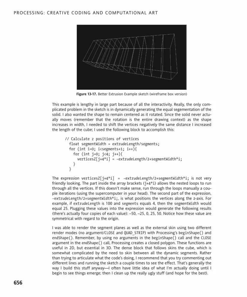
Figure 13-17. Better Extrusion Example sketch (wireframe box version)
This example is lengthy in large part because of all the interactivity. Really, the only com-plicated problem in the sketch is in dynamically generating the equal segementation of thesolid. I also wanted the shape to remain centered as it rotated. Since the solid never actu-ally moves (remember that the rotation is the entire drawing context) as the shapeincreases in width, I needed to shift the vertices negatively the same distance I increasedthe length of the cube; I used the following block to accomplish this:
// Calculate z positions of verticesfloat segmentWidth = extrudeLength/segments;for (int i=0; i<segments+1; i++){for (int j=0; j<4; j++){verticesZ[j+4*i] = -extrudeLength/2+segmentWidth*i;
}}
The expression verticesZ[j+4*i] = -extrudeLength/2+segmentWidth*i; is not veryfriendly looking. The part inside the array brackets (j+4*i) allows the nested loops to runthrough all the vertices. If this doesn’t make sense, run through the loops manually a cou-ple iterations (using the supercomputer in your head). The second part of the expression,-extrudeLength/2+segmentWidth*i;, is what positions the vertices along the z-axis. Forexample, if extrudeLength is 100 and segments equals 4, then the segmentWidth wouldequal 25. Plugging these values into the expression would generate the following results(there’s actually four copies of each value): –50, –25, 0, 25, 50. Notice how these value aresymmetrical with regard to the origin.
I was able to render the segment planes as well as the external skin using two differentrender modes (no argument/CLOSE and QUAD_STRIP) with Processing’s beginShape() andendShape(). Remember, by using no arguments in the beginShape() call and the CLOSEargument in the endShape() call, Processing creates a closed polygon. These functions areuseful in 2D, but essential in 3D. The dense block that follows skins the cube, which issomewhat complicated by the need to skin between all the dynamic segments. Ratherthan trying to articulate what the code’s doing, I recommend that you try commenting outdifferent lines and running the sketch a couple times to see the effect. That’s generally theway I build this stuff anyway—I often have little idea of what I’m actually doing until Ibegin to see things emerge; then I clean up the really ugly stuff (and hope for the best).
PROCESSING: CREATIVE CODING AND COMPUTATIONAL ART
656
617xCH13.qxd 4/18/07 3:24 PM Page 656

//render external skinfor (int i=0; i<segments+1; i++){beginShape(QUAD_STRIP);for (int j=0; j<4; j++){if (i<segments){vertex(verticesX[j+4*i], verticesY[j+4*i], verticesZ[j+4*i]);vertex(verticesX[j+4*i+4], verticesY[j+4*i+4], "
verticesZ[j+4*i+4]);if (j==3){//connnect last vertices back to beginning// to close formvertex(verticesX[4*i], verticesY[4*i], verticesZ[4*i]);vertex(verticesX[4*i+4], verticesY[4*i+4], "
verticesZ[4*i+4]);}
}}endShape();
}
Cube to pyramid to cone to cylinderMoving from a cube to a cylinder is very simple. In fact, you can even move from a cubeto a pyramid to a cone to a cylinder quite easily (see Figures 13-18 through 13-21).Watching this transmutation reveals the interesting interrelationship between these forms.The next example allows you to interactively shift between these forms in real time. Thecode implementation is yet another variation on what you’ve already looked at the lastfew examples, although the form-building algorithms are slightly different. Hopefullyyou’re beginning to see how certain implementations recur when you try to solve relatedproblems. One of the biggest advantages of OOP is the structural abstraction it providesfor handling these types of common implementations. Computer scientists refer to thesecommon implementations as design patterns. This is too big a topic to cover here, but youcan read more about it at www.patterndepot.com/put/8/JavaPatterns.htm.
Please note that this next sketch requires the Point3D class (not repeated following), butnot the Cube class. Without further ado, here’s the mutating Cube to Pyramid to Cone toCylinder sketch:
/*Cube to Pyramid to Cone to CylinderPoint3D class required******************************Instructions:Up Arrow -- increases pointsDown Arrow -- decreases points'p' key toggles between cube/pyramid*/
3D
657
13
617xCH13.qxd 4/18/07 3:24 PM Page 657

int pts = 4;float angle = 0;float radius = 115;float cylinderLength = 100;//verticesPoint3D vertices[][];boolean isPyramid = false;
void setup(){size(400, 400, P3D);noStroke();
}
void draw(){background(170, 95, 95);lights();fill(255, 200, 200);translate(width/2, height/2);rotateX(frameCount*PI/150);rotateY(frameCount*PI/130);rotateZ(frameCount*PI/180);
// initialize point arraysvertices = new Point3D[2][pts+1];
// fill arraysfor (int i=0; i<2; i++){angle = 0;for(int j=0; j<=pts; j++){vertices[i][j] = new Point3D();if (isPyramid){if (i==1){vertices[i][j].x = 0;vertices[i][j].y = 0;
}else {vertices[i][j].x = cos(radians(angle))*radius;vertices[i][j].y = sin(radians(angle))*radius;
}}else {vertices[i][j].x = cos(radians(angle))*radius;vertices[i][j].y = sin(radians(angle))*radius;
}vertices[i][j].z = cylinderLength;// the .0 after the 360 is criticalangle+=360.0/pts;
}cylinderLength*=-1;
}
PROCESSING: CREATIVE CODING AND COMPUTATIONAL ART
658
617xCH13.qxd 4/18/07 3:24 PM Page 658

// draw cylinder tubebeginShape(QUAD_STRIP);for(int j=0; j<=pts; j++){vertex(vertices[0][j].x, vertices[0][j].y, vertices[0][j].z);vertex(vertices[1][j].x, vertices[1][j].y, vertices[1][j].z);
}endShape();
//draw cylinder endsfor (int i=0; i<2; i++){beginShape();for(int j=0; j<pts; j++){vertex(vertices[i][j].x, vertices[i][j].y, vertices[i][j].z);
}endShape(CLOSE);
}}
/*up/down arrow keys controlpolygon detail.*/void keyPressed(){if(key == CODED) {// ptsif (keyCode == UP) {if (pts<90){pts++;
}}else if (keyCode == DOWN) {if (pts>4){pts--;
}}
}if (key =='p'){if (isPyramid){isPyramid=false;
}else {isPyramid=true;
}}
}// Point3D class required
3D
659
13
617xCH13.qxd 4/18/07 3:24 PM Page 659

Figure 13-18. Cube to Pyramid to Cone to Cylinder sketch (in the cube form)
Figure 13-19. Cube to Pyramid to Cone to Cylinder sketch (in the pyramid form)
PROCESSING: CREATIVE CODING AND COMPUTATIONAL ART
660
617xCH13.qxd 4/18/07 3:24 PM Page 660

Figure 13-20. Cube to Pyramid to Cone to Cylinder sketch (in the cone form)
Figure 13-21. Cube to Pyramid to Cone to Cylinder sketch (in the cylinder form)
3D
661
13
617xCH13.qxd 4/18/07 3:24 PM Page 661

If you haven’t figured it out by now, here’s how you mutate between the four forms:
1. Press the P key to convert from a cube to a pyramid.
2. Press and hold the up arrow key to convert from a pyramid to a cone.
3. Press the P key again to convert from a cone to a cylinder.
I was surprised by how easy it was to convert between these four forms. Prior to develop-ing this sketch, I had considered them (without really thinking much about it) as funda-mental, irreducible primitives, like the primary colors. I even managed to earn two artdegrees never realizing that a pyramid was just a cube with one of its faces collapsed to apoint.
The sketch should be fairly self-explanatory. However, there is one subtle point worth dis-cussing. When I first generated this sketch, it had an annoying bug. As the point countchanged, sometimes the geometry would get screwed up. I found a clever but overly com-plicated hack to solve the problem. However, when I was cleaning up the code, I realizedthat the problem was actually very simple to fix, and my complicated hack was a majorwaste of time (sort of a pattern in my life). The problem related to the line
angle+=360/pts;
which I resolved by changing it to
angle+=360.0/pts;
You have to look closely to even notice the difference between these two lines. Adding the.0 after the 360 solved the problem. Can you tell why? Originally, I thought the problemrelated to needing the point count to be a factor of 360, which does solve the problem.However, that was more of a symptom, not really the cause. The real problem was that Iwas using two int values in the 360/pts calculation, which not surprisingly produced anint; however, I needed a float value. By adding the .0 after the 360, the value was treatedas type float. Operations involving an int and a float will return a float. Thus, my anglecalculations, requiring float values, were getting rounded to int values, and I was slowlylosing accuracy, which screwed up the geometry. This may seem like an obscure point, butit is a pretty common error in programming and can be a nasty bug to track down.Sometimes rounding errors don’t show up for many iterations, as long as the error is smallenough. I recommend blaming the computer for these kinds of problems.
ToroidsBuilding upon the last few examples, it’s possible to put some of these ideas together tobuild slightly more complex forms, such as toroids and related forms (shown in Figures 13-22through 13-26). Toroids are ring forms (think inner tubes, bagels, or doughnuts). Toroidsalso have an interesting relationship to spheres and helixes, which you’ll see in the follow-ing example.
The algorithm for a regular toroid, where the cross-section shape is a circle and the toroidradius is constant, might be as follows:
PROCESSING: CREATIVE CODING AND COMPUTATIONAL ART
662
617xCH13.qxd 4/18/07 3:24 PM Page 662

1. Generate a circle (actually a polygon) on the xy plane at the origin (0, 0).
2. Displace the circle on the x-axis the distance of the toroid radius.
3. Copy (lathe) the circle elliptically around the y-axis, maintaining the toroid radiusdistance from the origin.
Toroids have a ring thickness, which relates to the initial diameter of the lathed circle, andan inner hole diameter based on the distance of the lathed circle from the origin. The ini-tial circle, which you’ll be lathing with, will actually be a polygon with a lot of points (likein the preceding cylinder example). Finally, the lathing will be controlled by a segmentlevel, which determines how many copies of the circle are rotated around the y-axis. Thelathe segments will be evenly spaced, and will determine the smoothness of the toroid.The really cool thing is that you can easily control all these properties in real time, inter-actively revealing a wide range of interesting 3D forms based on your initial algorithm. Thefollowing sketch includes a bunch of key commands, which are listed at the top of the pro-gram as a code comment. The sketch requires the Point3D class, but not the Cube class.
/* Interactive ToroidPoint3D class required
****************************************key command controls******************UP arrow key pts++;DOWN arrow key pts--;LEFT arrow key segments--;RIGHT arrow key segments++;'a' key toroid radius--;'s' key toroid radius++;'z' key initial polygon radius--;'x' key initial polygon radius++;'w' key toggle wireframe/solid shading'h' key toggle sphere/helix****************************************/
//ellipse (shape to lathe)int pts = 40;float angle = 0;float radius = 40.0;// lathe segmentsint segments = 60;float latheAngle = 0;float latheRadius = 100.0;//verticesPoint3D vertices[], vertices2[];// for shaded or wireframe renderingboolean isWireFrame = false;// for optional helixboolean isHelix = false;float helixOffset = 5.0;
3D
663
13
617xCH13.qxd 4/18/07 3:24 PM Page 663

void setup(){size(400, 400, P3D);
}
void draw(){background(50, 64, 42);// basic lighting setuplights();// 2 rendering styles// wireframe or solidif (isWireFrame){stroke(255, 255, 150);noFill();
}else {noStroke();fill(150, 195, 125);
}//center and spin toroidtranslate(width/2, height/2);
rotateX(frameCount*PI/150);rotateY(frameCount*PI/170);rotateZ(frameCount*PI/90);
// initialize point arraysvertices = new Point3D[pts+1];vertices2 = new Point3D[pts+1];
// fill arraysfor(int i=0; i<=pts; i++){vertices[i] = new Point3D();vertices2[i] = new Point3D();vertices[i].x = latheRadius + sin(radians(angle))*radius;if (isHelix){vertices[i].z = cos(radians(angle))*radius-(helixOffset* "
segments)/2;} else{vertices[i].z = cos(radians(angle))*radius;
}angle+=360.0/pts;
}
// draw toroidlatheAngle = 0;for(int i=0; i<=segments; i++){beginShape(QUAD_STRIP);for(int j=0; j<=pts; j++){if (i>0){
PROCESSING: CREATIVE CODING AND COMPUTATIONAL ART
664
617xCH13.qxd 4/18/07 3:24 PM Page 664

vertex(vertices2[j].x, vertices2[j].y, vertices2[j].z);}vertices2[j].x = cos(radians(latheAngle))*vertices[j].x;vertices2[j].y = sin(radians(latheAngle))*vertices[j].x;vertices2[j].z = vertices[j].z;// optional helix offsetif (isHelix){vertices[j].z+=helixOffset;
}vertex(vertices2[j].x, vertices2[j].y, vertices2[j].z);
}// create extra rotation for helixif (isHelix){latheAngle+=720.0/segments;
}else {latheAngle+=360.0/segments;
}endShape();
}}
/*left/right arrow keys control ellipse detailup/down arrow keys control segment detail.'a','s' keys control lathe radius'z','x' keys control ellipse radius'w' key toggles between wireframe and solid'h' key toggles between toroid and helix*/void keyPressed(){if(key == CODED) {// ptsif (keyCode == UP) {if (pts<40){pts++;
}}else if (keyCode == DOWN) {if (pts>3){pts--;
}}// extrusion lengthif (keyCode == LEFT) {if (segments>3){segments--;
}}
3D
665
13
617xCH13.qxd 4/18/07 3:24 PM Page 665

else if (keyCode == RIGHT) {if (segments<80){segments++;
}}
}// lathe radiusif (key =='a'){if (latheRadius>0){latheRadius--;
}}else if (key == 's'){latheRadius++;
}// ellipse radiusif (key =='z'){if (radius>10){radius--;
}}else if (key == 'x'){radius++;
}// wireframeif (key =='w'){if (isWireFrame){isWireFrame=false;
}else {isWireFrame=true;
}}// helixif (key =='h'){if (isHelix){isHelix=false;
}else {isHelix=true;
}}
}// Point3D class required
PROCESSING: CREATIVE CODING AND COMPUTATIONAL ART
666
617xCH13.qxd 4/18/07 3:24 PM Page 666
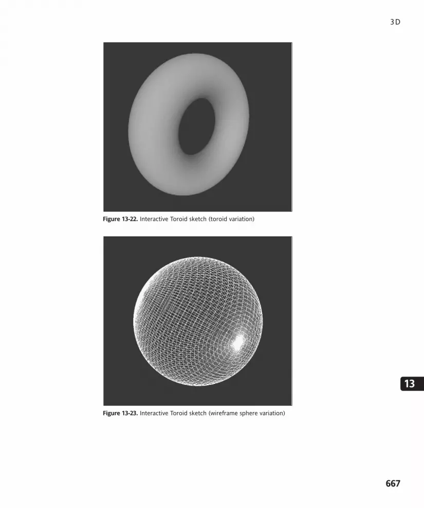
Figure 13-22. Interactive Toroid sketch (toroid variation)
Figure 13-23. Interactive Toroid sketch (wireframe sphere variation)
3D
667
13
617xCH13.qxd 4/18/07 3:24 PM Page 667

Figure 13-24. Interactive Toroid sketch (helix variation)
Figure 13-25. Interactive Toroid sketch (picture frame variation)
PROCESSING: CREATIVE CODING AND COMPUTATIONAL ART
668
617xCH13.qxd 4/18/07 3:24 PM Page 668

Figure 13-26. Interactive Toroid sketch (polyhedron variation)
If you haven’t yet, I suggest interacting with the toroid sketch. The four arrow keys and thekeys A, S, Z, and X can all be pressed and held down. The W and H keys can only bepressed and released. When playing with the sketch, you might try to make some of thefollowing forms: a bicycle inner tube, a monster truck inner tube, a picture frame, asawed-off pyramid, a sphere, a shell, a star, a braid, or part of a phone cord. Togglingbetween shaded and wireframe view (using the W key) makes it easier to see how thegeometry is changing.
Here’s how to make a sphere: press and hold the A key until the form stops collapsing.Make sure that you press the W key to see the wireframe. To increase the size of thesphere, press and hold the X key. Obviously, this is not the most efficient way to generatea sphere, but it’s interesting to see its relationship to the toroid. A more efficient way togenerate a sphere would be to create a 180-degree arc and then lathe it 360 degrees.
This sketch brings together many of the features covered earlier in this chapter. The majorchallenge was combining the point coordinate data used to generate the initial polygonwith the lathing of that data around the toroid. I used two separate arrays, vertices[] andvertices2[], to enable me to combine the data. The initial polygon (to be lathed) wasgenerated with the two lines of code used to plot a polygon in the xz plane:
vertices[i].x = latheRadius + sin(radians(angle))*radius;vertices[i].z = cos(radians(angle))*radius;
If I had plotted this initial polygon, it would have displayed only a horizontal line on theright side of the screen, since the y values are all 0 and the z dimension of the polygoncan’t be seen in the xy plane.
3D
669
13
617xCH13.qxd 4/18/07 3:24 PM Page 669

I then took this initial polygon data and lathed it around the z-axis, on the xy plane, withthe following expressions:
vertices2[j].x = cos(radians(latheAngle))*vertices[j].x;vertices2[j].y = sin(radians(latheAngle))*vertices[j].x;vertices2[j].z = vertices[j].z;
Notice that the equations are basically the original unit circle expressions, where the cos()function controls the x component of a point, the sin() function controls the y compo-nent, and vertices[j].x is the toroid radius value. Instead of a single point, though, I’mrotating a group of points that just happen to form a polygon on the xz plane.
The rest of the program is stuff I’ve gone over before. One small snippet that might raisea question, however, is the following:
if (isHelix){latheAngle+=720.0/segments;
}
I decided to rotate the helix version of the toroid two rotations instead of one, just to bet-ter illustrate the coil effect—that’s why I used 720.0 instead of 360.0. If you want, you canchange that number to see the effect. If you make it higher, you might also want to raisethe 80 segment level maximum in the conditional head if (segments<80). This will allowthe coil to remain smooth, if that sort of thing is important to you. Processing has a simple 3D function that does just this when creating a sphere. The function is calledsphereDetail(), and it works very similarly to the arrow keys in the last toroid example.Here’s a simple example (shown in Figure 13-27) to end the chapter on. Use the up anddown arrow keys to see the sphereDetail() function in action:
// sphereDetail() Exampleint detail = 10;int depth = 100;void setup(){size(400, 400, P3D);
}void draw(){background(50);translate(width/2, height/2, depth);rotateY(PI*frameCount/125);lights();fill(100, 50, 175);stroke(150, 75, 255);sphereDetail(detail);sphere(20);println(depth);
}
PROCESSING: CREATIVE CODING AND COMPUTATIONAL ART
670
617xCH13.qxd 4/18/07 3:24 PM Page 670

void keyPressed(){if(key == CODED) {if (keyCode == UP) {if (depth<310){depth+=20;detail+=2;
}}else if (keyCode == DOWN) {if (depth>70){depth-=20;detail-=2;
}}
}}
Figure 13-27. sphereDetail() Example sketch
If you play with the arrow keys, notice that the number of vertices making up the sphereincreases as the sphere grows in size (it actually stays the same size, but comes closer tothe screen on the z-axis), and vice versa. This represents another optimization approachused in 3D—only render the necessary resolution. Since the sphere is composed of trian-gles, when the sphere detail appears too low, the sphere loses its smooth, sphere-like qual-ity. I simply changed the sphere detail based on the sphere’s position on the z-axis. In thenext and final chapter, I’ll discuss a few other techniques for optimizing 3D, along withProcessing’s virtual camera and lighting functions.
3D
671
13
617xCH13.qxd 4/18/07 3:24 PM Page 671

SummaryCoding 3D, long the domain of hardcore programmers, is now accessible to the rest of us,thanks to Processing. One of the main difficulties in coding 3D has simply been gettingstarted. Most books on the subject are geared toward computer scientists, mathemati-cians, and engineers, and are filled with scary diagrams and equations. Just getting a sim-ple, static cube (a 3D primitive) on the screen can be an ordeal. This is not the case withProcessing, as the simple, ten-line rotating cube sketch at the beginning of the chapterrevealed. Using Processing’s handy pushMatrix() and popMatrix() functions, as shown inthe previous brick tower example, you can also easily construct more complex structures,combining simple 3D primitives.
This chapter went beneath the surface as well, revealing the usefulness of the same oldbasic trig functions you’ve been using throughout the book. You created your ownPoint3D, Cube, and SpinnyCube classes, with which you created a custom multicoloredcube and even coded your own 3D rotations. Building upon these classes with some sim-ple algorithms, you generated a larger set of 3D primitives, including a pyramid, cone,cylinder, toroid, and helix; and you explored how these forms are related through a fewinteractive sketches. Finally, you learned some 3D optimization techniques and looked atProcessing’s sphereDetail() function.
PROCESSING: CREATIVE CODING AND COMPUTATIONAL ART
672
617xCH13.qxd 4/18/07 3:24 PM Page 672

PART THREE REFERENCE
In Part 1 of the book, I covered general creative coding theory, and in Part 2, I demon-strated how the theory is implemented. This final part functions as sort of a Processingcheat sheet. Appendix A gives an overview of the Processing language reference;Appendix B contains some handy equations, as well as some important coding struc-tures and concepts; and Appendix C (available online) includes information on inte-grating the Processing core graphics library within Java. Keep in mind that the languagereference in Appendix A was designed to supplement the excellent official Processinglanguage reference—not to replace it.
617xAppA.qxd 4/26/07 10:57 AM Page 673

617xAppA.qxd 4/26/07 10:57 AM Page 674

A PROCESSING LANGUAGE API
617xAppA.qxd 4/26/07 10:57 AM Page 675

In this appendix, you will find a handy reference to all aspects of the Processing language,including many code examples to help you out and give you inspiration. This is the placeto come first if you want to quickly look up anything covered throughout the rest ofthe book.
Introducing the Processing APIThe Processing API is the reference for the core Processing language. This is the place tolook up a specific Processing command. The Processing API lives online at http://processing.org/reference/index.html, and a copy of it is also installed within your localProcessing application directory on your computer. The API is HTML-based with cross-referenced links throughout. There are also additional libraries available to Processing thatextend the language. The library reference is not included in the core language API.
The Processing core API can be viewed four different ways:
Abridged
Abridged (A–Z)
Complete
Complete (A–Z)
According to a blurb on the language reference page, the abridged reference “omitsdescription and functions for drawing in 3D and for detailed drawing and data manipula-tion.” The abridged and complete options (bullets 1 and 3) break the language down intological segments relating to basic command functionality. The two “A–Z” options lay thelanguage out alphabetically. Personally, I find the segmentation of the API by functioneasier to work with.
When you launch the reference site, the abridged viewing option is initially loaded.However, since in this chapter I’ll be discussing the complete API, you might want to selectthe complete option at first (before sending an angry e-mail to the publisher). To all younew coders, you don’t need to work with the entire API to use Processing. A lot of reallyinteresting things can be done with minimal amounts of code, using only a fraction of theAPI. As you progress, though, you’ll naturally begin to use more and more of the API, sodon’t worry about trying to cram or memorize all this stuff.
As I mentioned, it doesn’t make a lot of sense to me to re-create the entire API in thisbook when it is free to use, well organized, and easily accessible—both locally and at
Since there’s already an official reference available online and within your Processinginstallation, you might ask why I’ve written this appendix. Well, my intention was toexpand upon the more challenging concepts in the official reference, as well asinclude many additional code examples.
PROCESSING: CREATIVE CODING AND COMPUTATIONAL ART
676
617xAppA.qxd 4/26/07 10:57 AM Page 676

http://processing.org/. My main objective therefore is to briefly describe the overallorganization of the API and emphasize certain key issues. The rest of the book focuses oncode experiments that contextually move throughout the entire API, including some of thecore code libraries, which I’ll say more about at the end of this reference.
The complete (extended) API is segmented into 15 sections, which are further divided into45 subsections, with nearly 300 separate items, including functions, operators, constants,system variables, data types, and control structures. The 15 main sections are titled asfollows:
Structure
Environment
Data
Control
Shape
Input
Output
Transform
Lights, Camera
Color
Image
Rendering
Typography
Math
Constants
StructureThe nearly 30 items organized within the Structure section range from basic syntacticsymbols—such as comment structures ( // and /* */), parentheses, semicolons, and arraybrackets—to reserved language keywords, such as “class,” “this,” “true,” “super,” and“extends.” In addition, there are the Processing function calls setup(), size(), noLoop(),delay(), exit(), draw(), loop(), and redraw().
Structural elements in a programming language are used to organize the process ofcoding—a semicolon terminates a line, a dot connects an object to its properties andmethods, curly braces ({ }) organize a block of code, and so forth. Structure allows you tobuild, in a sense, sentences and stories with your code to visualize and express your ideas.I cover the concept of structure as it relates to general programming theory/practice inmore detail in Chapter 3.
PROCESSING LANGUAGE API
677
A
617xAppA.qxd 4/26/07 10:57 AM Page 677
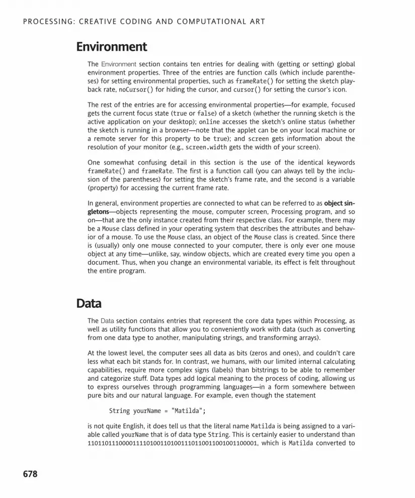
EnvironmentThe Environment section contains ten entries for dealing with (getting or setting) globalenvironment properties. Three of the entries are function calls (which include parenthe-ses) for setting environmental properties, such as frameRate() for setting the sketch play-back rate, noCursor() for hiding the cursor, and cursor() for setting the cursor’s icon.
The rest of the entries are for accessing environmental properties—for example, focusedgets the current focus state (true or false) of a sketch (whether the running sketch is theactive application on your desktop); online accesses the sketch’s online status (whetherthe sketch is running in a browser—note that the applet can be on your local machine ora remote server for this property to be true); and screen gets information about theresolution of your monitor (e.g., screen.width gets the width of your screen).
One somewhat confusing detail in this section is the use of the identical keywordsframeRate() and frameRate. The first is a function call (you can always tell by the inclu-sion of the parentheses) for setting the sketch’s frame rate, and the second is a variable(property) for accessing the current frame rate.
In general, environment properties are connected to what can be referred to as object sin-gletons—objects representing the mouse, computer screen, Processing program, and soon—that are the only instance created from their respective class. For example, there maybe a Mouse class defined in your operating system that describes the attributes and behav-ior of a mouse. To use the Mouse class, an object of the Mouse class is created. Since thereis (usually) only one mouse connected to your computer, there is only ever one mouseobject at any time—unlike, say, window objects, which are created every time you open adocument. Thus, when you change an environmental variable, its effect is felt throughoutthe entire program.
DataThe Data section contains entries that represent the core data types within Processing, aswell as utility functions that allow you to conveniently work with data (such as convertingfrom one data type to another, manipulating strings, and transforming arrays).
At the lowest level, the computer sees all data as bits (zeros and ones), and couldn’t careless what each bit stands for. In contrast, we humans, with our limited internal calculatingcapabilities, require more complex signs (labels) than bitstrings to be able to rememberand categorize stuff. Data types add logical meaning to the process of coding, allowing usto express ourselves through programming languages—in a form somewhere betweenpure bits and our natural language. For example, even though the statement
String yourName = "Matilda";
is not quite English, it does tell us that the literal name Matilda is being assigned to a vari-able called yourName that is of data type String. This is certainly easier to understand than1101101110000111101001101001110110011001001100001, which is Matilda converted to
PROCESSING: CREATIVE CODING AND COMPUTATIONAL ART
678
617xAppA.qxd 4/26/07 10:57 AM Page 678

its binary equivalent. I used some of the commands in this section of the API to generatethe Matilda bitstring. Here’s the code I ran:
int m = int(‘M’);int a = int(‘a’);int t = int(‘t’);int i = int(‘i’);int l = int(‘l’);int d = int(‘d’);println(binary(m)+binary(a)+binary(t)+binary(i)+ !
binary(l)+binary(d)+binary(a));
The five subsections of Data are as follows:
Primitive
Composite
Conversion
String Functions
Array Functions
PrimitivePrimitive includes data types used to store individual values—for example, int nodeCount= 6; or float speed = .5;. As discussed already, variables in Processing and Java need tobe declared of a specific type. Types specify the kind of data a variable can hold and alsothe limit to the size of the value they can hold. Primitive variables are also assigned valuesdirectly. In the statement float speed = .5;, the real value .5 is literally assigned to thevariable speed.
There are also reference variables in Processing and Java, in which a variable is notassigned a direct value, but rather the address in memory to where the value is stored. Thisstrange-sounding arrangement is also referred to as a pointer in other languages. Sinceobjects, as well as arrays (which hold multiple values), are complex structures, it makessome sense to store a reference to the data, rather than the actual data.
The Processing primitive data types are a subset of Java’s primitive data types. Java has afew more subtle variations on the main ones in Processing that most beginning coders canavoid. However, you are free to use Java’s extra data types in Processing if you’d like.Finally, there is a primitive data type in Processing that is not in Java: the color data type.This Processing type is really just an int type in disguise, used to deal specifically withcolor values. Appendix B includes detailed technical information about the inner workingsof Processing’s color data type.
Fortunately, actually using primitives in Processing is a lot simpler than trying to under-stand my theoretical, long-winded description of them. I go into greater depth about vari-ables and data types in Chapter 3, and I also cover color in more detail toward the end ofthis chapter, as well as in Chapter 4.
PROCESSING LANGUAGE API
679
A
617xAppA.qxd 4/26/07 10:57 AM Page 679

CompositeThe Composite section includes data types used to store object references (the memoryaddresses I mentioned in the primitive data type discussion). The three composite typesArray, Object, and String can each hold multiple pieces of data.
Arrays are collections of any other data type, referenced by a single variable name. Arrayscan only hold one data type at a time, but lots of it. I cover arrays in detail in Chapter 3.
Objects are the main units in object-oriented programming. An object is an instance of aclass and includes copies of the properties and methods defined within the class. Objectsare covered in much greater depth in Chapter 8 in the discussion of object-oriented pro-gramming (OOP).
Strings are kind of like arrays that only hold characters (e.g., letters). There are two waysto create String objects in Processing and Java (which is confusing):
String s1 = "hello";
and
String s2 = new String("hello");
The first way looks like a normal primitive declaration, like you would use to declare anint (int count = 3;), a float (float speed = .5;), and so on. The second way looks likestandard object creation, called instantiation, which uses the standard object-oriented syn-tax ClassType variableName = new ClassType();. Based on what I’ve told you aboutdata types up to this point in the book, this may not make sense. How can a string repre-sent both a primitive data type and also a reference (composite) data type? Well, in truth,there is no primitive String data type in Java or Processing; you’re always creating aString object. The shortcut approach String s1 = "hello"; internally creates a Stringobject from the literal (the word in quotes). This is all fine and good, as well as probably alittle overly technical. However, if you eventually find yourself needing to compare twostrings and test them for equality, these two different string-creation approaches havesome confusing (and probably annoying) differences.
As an example, run the following:
String s1 = "hello";String s2 = new String("hello");println(s1 == s2);
String s3 = "goodbye";String s4 = "goodbye";println(s3 == s4);
The output tells you that s1 and s2 are not equal, but s3 and s4 are. Even though the twovalues being compared in each comparison are the same (hello and hello and goodbyeand goodbye), the output is different because of the different ways the strings were cre-ated. I won’t bore you further with why this occurs, but you can read more about it here:http://java.about.com/library/weekly/aa_strings1.htm. Be sure to check the second
PROCESSING: CREATIVE CODING AND COMPUTATIONAL ART
680
617xAppA.qxd 4/26/07 10:57 AM Page 680

part of the article as well. My suggestion when creating strings is to use the shortcutapproach. If for some reason you do need to compare the values of two strings createdusing the object-oriented approach (using the new keyword), you can use Java’s Stringmethod equals(). Here’s an example:
String s1 = new String("hello");String s2 = "hello";println("s1 == s2 is " + (s1 == s2));println("s1.equals(s2) is " + s1.equals(s2));
String s3 = new String("goodbye"); String s4 = new String("goodbye");println("s3 == s4 is " + (s3 == s4));println("s3.equals(s4) is " + s3.equals(s4));
ConversionThe Conversion section includes ten entries, each of which is a utility function for convert-ing between one data type and another. Since variables hold values of a specific type,there are times when, for example, you may need to use a value of type float to pass intoa function that requires an integer value. Processing has a way of doing this conversion,called type casting. For example, to convert a float variable named gpa to an integer, youjust need to write int(gpa). One issue to consider when doing conversion is truncation. Inmy example, the gpa float value will be truncated, or shortened, when it is converted. Forexample, if gpa equals 3.97, after converting it using int(gpa), the value returned will be3 (not 4). Instead of rounding the value, it simply snips off all the values to the right of thedecimal point. Thus, a simple data conversion mistake like this could keep you out of gradschool. There are of course other and better ways to solve this last example (involving log-ical value rounding), which I’ll cover later in my discussion of the Math section.
There’s one final cautionary note about using Processing’s int() and float() conversionfunctions. Currently, there is a reported and unresolved bug about their use(http://dev.processing.org/bugs/show_bug.cgi?id=4). Thus, if these functions don’tseem to be working, it’s recommended that you use Java’s alternative syntax. Here’s anexample:
float temp = 98.64783;//Processing conversion syntaxint pTemp = int(temp);println(pTemp);//Java conversion syntaxint jTemp = (int)temp;println(jTemp);
PROCESSING LANGUAGE API
681
A
617xAppA.qxd 4/26/07 10:57 AM Page 681

String FunctionsThe String Functions section has seven functions that are helpful when working withstrings, including join(), which combines elements in an array into a string; nf(), whichformats numbers into strings; and split(), which separates a series of data within a stringinto separate arrays of strings. Here’s a little example using the String function trim(),which removes whitespace characters around strings:
String s1 = " Hi there, ";String s2 = " bye now. ";println(s1+s2);s1 = trim(s1);s2 = trim(s2);println(s1+" "+s2);
Array FunctionsThe Array Functions section includes nine functions that allow you to manipulate arrays. InJava, the size of an array can’t be changed once its length has been set. Values at specificindex positions within arrays can easily be changed—as in scores[3] = 23; or names[4]= "Bella";—and there are ways of easily sorting and searching though arrays (see Java’sArrays class). However, in Java, if you want to change the length of an array, you need tocopy the contents of the array into a new array that has been initialized with the newdesired length (too much work). I’ll provide an example of this process later in this section.
There are two additional classes in Java, ArrayList and Vector, that (sort of) function asmutable arrays, in that they can dynamically change size. However, using these more com-plex structures necessitates converting data types (type casting, which I discussed a coupleparagraphs back), and also requires some extra syntax (which I’m not going to cover here).To learn more about Java’s mutable array structures, check out http://java.sun.com/j2se/1.4.2/docs/api/java/util/Vector.html.
Processing arrays, in conjunction with the array functions, are a hybrid solution—retainingthe simplicity of using a standard Java array while also providing the ability to modify thearray (including altering its length), similar to Java’s ArrayList and Vector classes.
Processing’s array functions include append() and shorten(), which respectively add orsubtract data to or from the end of an array, changing the array’s length by one position;splice(), which adds a single value or an entire array of values into an array at a specificindex position, also changing the length of the array by the number of total values added;and subset(), which extracts an array of elements out of an array at a specific index posi-tion. The subset() function doesn’t affect the initial array.
In the following sections, I’ve included some example implementations of an append()function. The first sketch example demonstrates the long way to append, as you mightusing Java arrays. The second example uses Processing’s built-in append() function. Finally,the third example uses Processing’s append() function again, but with an array full ofobject references instead of primitive values.
PROCESSING: CREATIVE CODING AND COMPUTATIONAL ART
682
617xAppA.qxd 4/26/07 10:57 AM Page 682

Example 1: A Java approachvoid setup(){// before appendingint[]a = {2, 4, 5, 9, 13, 17, 20};print("before myAppend a = ");for (int i=0; i<a.length; i++) {print(a[i]+" ");
}//after appendinga = myAppend(a, 23);print("\nafter myAppend a = ");for (int i=0; i<a.length; i++) {print(a[i]+" ");
}}/*Java append implementation -- doing it the long way.An array and new value are passed to the myAppend()function, which copies the passed in array values into anew array, with a length 1 greater than the passed in array.Then the passed in valueToAdd argument is assignedto the added index position in the new array*/int[] myAppend(int[]ar1, int valueToAdd){int length = ar1.length;int[]ar2 = new int[length+1];for (int i=0; i<length; i++){ar2[i] = ar1[i];
}ar2[length] = valueToAdd;return ar2;
}
Example 2: Using Processing’s append() function, the easy way
// before appendingint[]a = {2, 4, 5, 9, 13, 17, 20};print("before append a = ");for (int i=0; i<a.length; i++) {print(a[i]+" ");
}//after appendinga = append(a, 23);print("\nafter append a = ");for (int i=0; i<a.length; i++) {print(a[i]+" ");
}
PROCESSING LANGUAGE API
683
A
617xAppA.qxd 4/26/07 10:57 AM Page 683

Example 3: Using Processing’s append() function on anarray of objects
// type casting requiredvoid setup(){SimpleClass[] sc = {new SimpleClass(), new SimpleClass(), !
new SimpleClass()};println("sc length before append = " + sc.length);// I need to explicitely cast the returned Object array !
to a SimpleClass arraysc = ((SimpleClass[])append(sc, new SimpleClass()));print("sc length after append = " + sc.length);
}class SimpleClass{}
This third example requires some understanding of OOP, which is covered in detail inChapter 8.
The last line in the example is the definition for a class (which has no capabilities at all, butis a valid class nonetheless). Since a class is a legal data type, it’s OK for me to declare anarray of type SimpleClass, as I did in this line:
SimpleClass[] sc = {new SimpleClass(), new SimpleClass(), !new SimpleClass()};
I also filled the array with three SimpleClass objects when I declared it. Every time newSimpleClass() is called, a SimpleClass object is returned between the curly braces. Thus,the sc array holds three SimpleClass object references. The first println() statementconfirms this. Next, I call Processing’s append() function, which is where the type castingoccurs. If I had tried to call the append() function as I did in the previous example—likethis:
sc = append(sc, new SimpleClass());
I’d get an error to the effect that I can’t assign an array of type Object to a variable oftype SimpleClass[]. The reason that the append() function converts the originalSimpleClass[] array to type Object relates to how the append() function works inter-nally, which I won’t go into. The way to fix this type mismatch is to explicitly type cast theObject array back to SimpleClass[], as I did in this line:
sc = ((SimpleClass[])append(sc, new SimpleClass()));
ControlThe Control section includes 18 entries divided in four sections. Control elements inProgramming are the logic constructs that control how a program flows, as well as, in thecase of loops, the data processing mechanisms supplying power and iterative efficiency.
PROCESSING: CREATIVE CODING AND COMPUTATIONAL ART
684
617xAppA.qxd 4/26/07 10:57 AM Page 684

The combination of these two structures that control program flow and processingefficiency are what make most of the cool things we do with computers possible; an exam-ple might be the photorealistic effects in big-budget animated features, such as naturallymoving fur on a virtual animal. To the computer, the fur is just a large array of coordinateschanging over time, based on expressions and conditional logic—of course, this is a loteasier said than done. The Control section is divided into the following four subsections:
Relational Operators
Iteration
Conditionals
Logical Operators
Relational OperatorsRelational operators function by Boolean logic—the condition being assessed is either trueor false. These six operators include < (less than), <= (less than or equal to), == (equals),and their respective opposites. These operators are used in the heads of conditional state-ments, where a true condition is tested for. Based on the outcome of the conditional test,program flow continues either within the conditional block (true) or past it (false).
IterationThe Iteration section includes just two entries, for() and while(). These are loop struc-tures within Processing and Java that allow for efficient processing of large quantities ofdata. Loops are essential to programming, and programs of even modest complexity willalmost always utilize them. However, loops can also be a little confusing when you are juststarting out, as programming logic can get more densely packed in loops and look a littleintimidating. It is also possible (and very common practice) to nest loops, in which a loopis put within another loop. This is often an efficient solution, but it adds complexity to thelook and logic of the structure. Since loops are great at processing large amounts of data,they are often used in conjunction with arrays. Following, I’ve included three examples(shown in Figures A-1 through A-3) to help illustrate both the power and complexity ofloops. The first example doesn’t use a loop, but simply creates three rectangles, spacingthem evenly in the display window. The second example uses a while loop to space tenrectangles evenly in the window. The third example, which is a lot more complicated, usesa bunch of for loops, including a nested for loop, to create a honeycomb structure.
Example 1: Spacing rectangles the hard way// create 3 rectangles// without loopsize(200, 200);int rects = 3;int w = width/rects;int h = w;
PROCESSING LANGUAGE API
685
A
617xAppA.qxd 4/26/07 10:57 AM Page 685

int x = 0;int y = height/2-h/2;rect(x, y, w, h);rect(x+w, y, w, h);rect(x+w*2, y, w, h);
Figure A-1. Create 3 Rectangles sketch
Example 2: Spacing rectangles the easy way // Use a loop to create 10 rectanglessize(200, 200);int rects = 10;int w = width/rects;int h = w;int x = 0;int y = height/2-h/2;int i = 0;while (i++<rects){rect(x, y, w, h);x+=w;
}
Figure A-2. Use a Loop to Create 10 Rectangles sketch
PROCESSING: CREATIVE CODING AND COMPUTATIONAL ART
686
617xAppA.qxd 4/26/07 10:57 AM Page 686

Example 3: Creating a honeycomb gradient/*HoneyCombIra Greenberg, November 6, 2005*/
// total polysint polyCount;// poly arrayPoly[]pols;// I created 2 radii to allow asymmetryint rad1 = 10, rad2 = 10;// change poly orientationfloat initAng = 0;
void setup(){size(400, 400);background(255);/* 1 extra cell is added to each row andcolumn to allow the honeycomb to bleedoff the display window */polyCount = (width/(rad1*2) + 1) * (height/(rad2*2) + 1);//create Poly arraypols = new Poly[polyCount];
for (int i=0; i<polyCount; i++){// instantiate each Poly obj in pols arraypols[i] = new Poly(6, rad1, rad2, initAng);
}}
void draw(){background(255);// counter keeps track of Poly countint counter = 0;// shift creates honeycomb pattern// and bleedint shiftx = rad1/2;int shifty = rad2/2;/* create rows and columns in honeycomb,calling Poly drawPoly method for eachPoly obj*/for (int i=shiftx; i<=width+shiftx; i+=rad1*2){shifty*=-1;for (int j=shifty; j<=height+shifty; j+=rad2*2){pols[counter++].drawPoly(i, j);
}}
}
PROCESSING LANGUAGE API
687
A
617xAppA.qxd 4/26/07 10:57 AM Page 687

/*Simple Poly class, plots any regular polygon*/class Poly {int sides;float r1, r2;float angle;
Poly(int sides, int r1, int r2, float initAng){this.sides = sides;this.r1 = r1;this.r2 = r2;angle = initAng;
}
void drawPoly(int cx, int cy){noStroke();fill(cy, cx, 100);float px= 0, py = 0;beginShape();for (int i=0; i<sides; i++){px = cx+cos(radians(angle))*r1;py = cy+sin(radians(angle))*r2;vertex(px, py);angle+=360/sides;
}endShape(CLOSE);
}}
Figure A-3. HoneyComb sketch
PROCESSING: CREATIVE CODING AND COMPUTATIONAL ART
688
617xAppA.qxd 4/26/07 10:57 AM Page 688
ConditionalsConditionals and the relational operators work together. The seven entries in theConditionals section are the words/structures used in conjunction with the operators (<, >=,etc.). The two most commonly used conditionals, especially by new coders, are the if()structure and the reserved keyword else. When used together, along with the operators,this simple if...else structure become a powerful data logic tool. There are also twoother structures: case, used for switch statements, and ?:, a condensed version of theif...else structure—which are variations on this important programming construct. Icover these structures, including some examples, in Chapter 3.
Logical OperatorsThe Logical Operators section includes just three entries: !, &&, and ||, which are “not”,“and,” and “or,” respectively. These operators allow you to make compound conditionalstatements, in which more than one condition can be checked within the same structure.Using these logical operators in conjunction with the other structures in the Control sec-tion—relational operators, loops, and conditionals—you can control the world (or at leastmake some interesting code art).
The next example, which depicts population explosion, includes some relational and logi-cal operators (see Figure A-4). Breeding in this simple world is caused by the bots collidingwith the edges of the display window. The detectCollision() function utilizes two com-pound conditional expressions. Notice how I divided the sketch up into a series of func-tions, with each function handling a specific task; this modular approach makes theprogram easier to understand.
/* Population ExplosionIra Greenberg, November 6, 2005revised October 10, 2006 */
//declare some global variablesint botCount = 0;int botLimit = 1000;color worldColor = color(0, 40);color[] botColor = new color[botCount];float[] x = new float[botCount];float[] y = new float[botCount];float[] speedX = new float[botCount];float[] speedY = new float[botCount];float botSize = 3;
void setup(){size(400, 400);smooth();noStroke();breedBot();
}
PROCESSING LANGUAGE API
689
A
617xAppA.qxd 4/26/07 10:57 AM Page 689

void draw(){fill(worldColor);rect(0, 0, width, height);birthBot();moveBot();detectCollision();
}
// expand arraysvoid breedBot(){if (botCount<1000){botCount++;// expand arraysx = append(x, width/2);y = append(y, height/2);speedX = append(speedX, random(-3, 3));speedY = append(speedY, random(-3, 3));botColor = append(botColor, color(random(200, 255), !random(127), random(40), random(100, 255)));
}}
// draw botsvoid birthBot(){for (int i=0; i<botCount; i++){fill(botColor[i]);ellipse(x[i], y[i], botSize, botSize);
}}
// animate botsvoid moveBot(){for (int i=0; i<botCount; i++){x[i]+=speedX[i];y[i]+=speedY[i];
}}
// check boundary collisionsvoid detectCollision(){for (int i=0; i<botCount; i++){// right and left boundariesif (x[i] >= width-botSize/2 || x[i] <= botSize/2){// reverse directionspeedX[i]*=-1;// make new botbreedBot();
}
PROCESSING: CREATIVE CODING AND COMPUTATIONAL ART
690
617xAppA.qxd 4/26/07 10:57 AM Page 690

// top and bottom boundariesif (y[i] >= height-botSize/2 || y[i] <= botSize/2){// reverse directionspeedY[i]*=-1;// make new botbreedBot();
}}
}
Figure A-4. Population Explosion sketch
ShapeThe 30-plus entries in the Shape section are all function calls involved in drawing geome-try. This section is the meat and potatoes of the API, especially with regard to the creativestuff beginning coders need to know. Most computer languages contain the other con-structs I’ve gone over thus far—structural elements, data storage, looping, conditionals,and so forth. However, many lack extensive drawing methods, and almost none containthe ease-of-use and full-featured capabilities of Processing’s drawing methods, which eveninclude a custom 3D engine. Java does have extensive drawing capabilities, but the Javagraphics APIs are complex, and something as simple as getting a rectangle to move acrossthe screen can bring new (and even experienced) coders to their knees. Shape is dividedinto the following five sections:
PROCESSING LANGUAGE API
691
A
617xAppA.qxd 4/26/07 10:57 AM Page 691

2D Primitives
Curves
3D Primitives
Attributes
Vertex
2D Primitives2D primitives are the basic geometric building blocks. They include points, lines, triangles,rectangles, arcs, and ellipses. Shapes like squares and circles are just variations on rectan-gles and ellipses. These functions are incredibly easy to use and fun to experiment with. Asyou’ll learn eventually, all shapes are really just points, or vertices connected and option-ally filled. However, it makes it really convenient to encapsulate this process for the basicbuilding block shapes into neat functions, like the ones in Processing. Here’s a simpleexample of a point inside a triangle, inside a rectangle, inside an ellipse (see Figure A-5):
size(200, 200);background(255);smooth();noFill();point(width/2, height/2);triangle(40, 160, 100, 40, 160, 160);rect(40, 40, 120, 120);ellipse(width/2, height/2, 120, 120);
Figure A-5. Processing’s 2D primitive functions
PROCESSING: CREATIVE CODING AND COMPUTATIONAL ART
692
617xAppA.qxd 4/26/07 10:57 AM Page 692

You’ll notice that by default, the rectangle is drawn from its top-left corner while theellipse is drawn from its center. If this doesn’t seem to make any sense, look at the differ-ent x and y positions for these shapes (the first two arguments). You can also explicitlychange how these shapes are drawn, if the default doesn’t work for you, with calls toeither rectMode() or ellipseMode(). These two functions can take a couple differentarguments that control how the shape is drawn. For example, to reverse the default modesfor both the rect() and ellipse() functions, you would write rectMode(CENTER); andellipseMode(CORNER);, respectively. Now rectangles would be drawn from the center andellipses would be drawn from the top-left corner.
CurvesThe Curves section includes eight entries, dealing with—you guessed it—creating curves.Curves are a lot more difficult to draw than rectilinear shapes. If you don’t believe me, justtry drawing a circle freehand. Our brains and physical capabilities seem more equipped todeal with simple linear ratios than curvy math. Unfortunately, most really interesting formsand animations tend to deal with more organic-looking structures and dynamics. The twomain curve drawing functions in Processing are bezier() and curve().
Bézier curves require two anchor points and two control points. The control points, in asense, direct the curve between the anchor points. The common pen tools in programslike Illustrator and Photoshop employ Bézier-like curves, allowing you to interactively con-trol both the anchor points and their control handles.
The curve() function utilizes a spline curve and also requires two extra control points.However, spline curves react quite differently from Bézier curves when these controlpoints are manipulated. In the next code example, you can drag the control and anchorpoints on two different curves simultaneously to see this difference (see Figure A-6). Thegreen path is a spline curve and the blue is a Bézier curve. Notice how the control pointsfor the Bézier curve are off the curve, while with the spline the control points are directlyon the curve. This is a pretty advanced example, which I included to illustrate how thecurves work. I cover the curve functions in detail in Chapter 7.
/*CurvesIra Greenberg, November 7, 2005revised October 9, 2006--------------------------------------Interact with the curves by draggingthe anchors/control pointsgreen curve = splineblue curve = bezier*/
int pts = 4;int ptSize = 6;float[]x = new float[4];float[]y = new float[4];boolean[]isDragSafe = new boolean[4];
PROCESSING LANGUAGE API
693
A
617xAppA.qxd 4/26/07 10:57 AM Page 693

void setup(){size(300, 300);smooth();// fill coordinate arraysx[0] = x[1] = 50;x[2] = x[3] = width-50;y[0] = height/2-50;y[3] = height/2+50;y[1] = y[2] = height/2;
//initialize dragging flags to falsefor (int i=0; i<pts; i++){isDragSafe[i] = false;
}}
void draw(){background(255);noFill();//draw curves and control handlesstrokeWeight(2);//spline curvestroke(0, 200, 30);curve (x[0], y[0],x[0], y[0], x[1], y[1], x[2], y[2]);curve (x[0], y[0], x[1], y[1], x[2], y[2], x[3], y[3]);curve (x[1], y[1], x[2], y[2], x[3], y[3], x[0], y[0]);//bezier curvestroke(0, 30, 200);bezier (x[1], y[1],x[0], y[0], x[3], y[3], x[2], y[2]);// draw bezier handlesstrokeWeight(1);stroke(100);line(x[0], y[0], x[1], y[1]);line(x[2], y[2], x[3], y[3]);// draw anchor/control pointsstroke(0);fill(0);for (int i=0; i<pts; i++){if (i==0 || i==3){fill(255, 100, 10);rectMode(CENTER);rect(x[i], y[i], ptSize, ptSize);
}else {fill(0);ellipse(x[i], y[i], ptSize, ptSize);
}}
PROCESSING: CREATIVE CODING AND COMPUTATIONAL ART
694
617xAppA.qxd 4/26/07 10:57 AM Page 694

// start dragging if flag truefor (int i=0; i<pts; i++){if (isDragSafe[i]){x[i] = mouseX;y[i] = mouseY;
}}
}
// release any point attached to the mousevoid mouseReleased (){for (int i=0; i<pts; i++){isDragSafe[i] = false;
}}
// for dragg'n dem pointsvoid mousePressed (){for (int i=0; i<pts; i++){if (mouseX>=x[i]-5 && mouseX<=x[i]+ptSize+5 && mouseY>=y[i]-5 && mouseY<=y[i]+ptSize+5){isDragSafe[i] = true;
}}
}
// show hand when over draggable pointsvoid mouseMoved (){cursor(ARROW);for (int i=0; i<pts; i++){if (mouseX>=x[i]-5 && mouseX<=x[i]+ptSize+5 && mouseY>=y[i]-5 && mouseY<=y[i]+ptSize+5){cursor(HAND);
}}
}
Figure A-6. Curves sketch
PROCESSING LANGUAGE API
695
A
617xAppA.qxd 4/26/07 10:57 AM Page 695

3D PrimitivesThe 3D Primitives section only includes three functions:
box()
sphere()
sphereDetail()
The box() and sphere() functions generate simple 3D objects. These are not simulated 3Dforms, but are actually based on 3D geometry. Thus, to use these functions, you need tospecify either the P3D or OPENGL rendering mode in the size() function call. If you useOPENGL, you also need to import the OPENGL library (via the Sketch " Import Library "opengl menu option).
The SphereDetail() function controls the level of detail, or number of vertices, used togenerate the sphere, which is constructed out of triangles that all fit together in a mosaicpattern (called tessellated triangles). Here’s a little example of some spinning stuff, usingall three of the 3D primitive functions (see Figure A-7). The outer ring of spheres in theexample illustrates the use of the sphereDetail() function. Each of the objects in the ringis technically a sphere, but by setting the sphereDetail value very low, you get a morerigid, less sphere-like form.
/* Spinning 3D StuffIra Greenberg, October 9, 2006 */float px, py, angle;void setup(){size(400, 400, P3D);noFill();stroke(255);
}void draw(){background(0);translate(width/2, height/2);pushMatrix();rotateY(frameCount*PI/150);rotateX(frameCount*PI/150);box(100, 100, 100);pushMatrix();rotateY(-frameCount*PI/10);rotateX(PI/4);box(45, 15, 65);
popMatrix();popMatrix();
PROCESSING: CREATIVE CODING AND COMPUTATIONAL ART
696
617xAppA.qxd 4/26/07 10:57 AM Page 696

pushMatrix();rotateY(-frameCount*PI/60);rotateX(-frameCount*PI/70);for (int i=0; i<12; i++){px = cos(radians(angle))*150;py = sin(radians(angle))*150;pushMatrix();translate(px, py);sphereDetail(i);sphere(20);
popMatrix();angle+=360/12;
}popMatrix();
}
Figure A-7. Spinning 3D Stuff sketch
PROCESSING LANGUAGE API
697
A
617xAppA.qxd 4/26/07 10:57 AM Page 697

AttributesThe Attributes section includes seven functions:
strokeWeight()
smooth()
strokeJoin()
noSmooth()
ellipseMode()
rectMode()
strokeCap()
Stroke is the term used for a line in computer graphics. The functions strokeWeight(),strokeCap(), and strokeJoin() respectively control the thickness (or weight) of lines,how the lines end (rounded, square, or extended caps), and how the lines come togetherat corners (mitered, beveled, or rounded). These last two line attributes are details wetend not to focus on until we see a problem with our output, and then of course weobsess about them.
smooth() and noSmooth() control anti-aliasing. Anti-aliasing is not a political position, buta way to smooth jaggies along curved and diagonal edges. Anti-aliasing makes things looksmoother, but can slow down rendering some. Please note that the smooth and strokeattribute functions do not (as of this writing) work consistently in all three supported ren-derers; nor do they fail consistently—the strokeWeight() attribute fails silently in P3Dmode (it just won’t do anything), but the other functions will generate a compiler error.For more details, please see the corresponding section of the API (www.processing.org/reference/strokeWeight_.html).
VertexThe Vertex section includes seven functions that allow you to do some pretty amazingthings. A vertex is just a point. Vertices (the plural form of vertex) make up lines, whichmake up polygons (usually triangles or quadrangles), which make up more complex geom-etry. In fact, most complex 3D scenes are usually just a bunch of triangles and quadrangles.To create a vertex in Processing, you use the vertex() function. Combining a series ofvertex() commands allow you to create lines and shapes (both 2D and 3D). Additionally,you can use the related functions bezierVertex() and curveVertex() to specify curves,and you can also combine the three commands.
The vertex functions need to be called between the functions beginShape() andendShape(). These two functions work by first internally recording the coordinates speci-fied by the nested vertex calls, and then plotting the coordinates. They also control howthe vertices are connected by passing arguments to the two calls. For example, here’ssome code to generate a closed regular polygon:
PROCESSING: CREATIVE CODING AND COMPUTATIONAL ART
698
617xAppA.qxd 4/26/07 10:57 AM Page 698

// regular polygonsize(400, 400);smooth();float px, py, angle = 0, radius = 150;int sides = 8;beginShape();for (int i=0; i<sides; i++){px = width/2+cos(radians(angle))*radius;py = height/2+sin(radians(angle))*radius;vertex(px, py);angle+=360.0/sides;
}endShape(CLOSE);
By default, beginShape() and endShape() will fill the shape created by the vertices.However, the shape will not actually be closed unless the CLOSE argument is included inthe endShape(CLOSE) call. Try removing the CLOSE argument from the last sketch and alsoadding the call noFill() above beginShape(). If you run the sketch, you should see a par-tial polygon drawn, with one of its sides missing. If you now remove noFill(), the fill ofthe shape will return, but the stroke outline surrounding the polygon will remain unclosed.There are a number of arguments that can be added to the beginShape() call, includingPOINTS, LINES, TRIANGLES, TRIANGLE_FAN, TRIANGLE_STRIP, QUADS, and QUAD_STRIP.
In addition, using the P3D and OPENGL rendering modes, it’s possible to map an imageonto a shape’s surface (really the shape’s vertices) using extra coordinate argumentspassed into the individual vertex() commands. It’s also necessary to include two addi-tional function calls: textureMode() and texture(). This is an advanced feature called UVmapping. The U and V represent two extra coordinates for the image mapping space onthe surface. Even though it’s an advanced feature, it’s also pretty cool, so I decided toinclude an example.
The sketch is of a rotating cube mapped with six images that rotate with the cube (seeFigure A-8). To try this example, you’ll need to create a data directory within your sketchfolder that contains six images named img1.jpg through img6.jpg. The data directory willbe created automatically when you import your images (by selecting Add File from theSketch menu). I suggest making the images each 250 by 250 pixels, but other sizes willwork as well.
/*ImageMapIra Greenberg, November 4, 2005revised, October 10, 2006*/
/* IMPORTANT- to run this, you need 6 images in your data directory namedimg1.jpg - img6.jpg. Images should eachbe 250 x 250 pixels */
PROCESSING LANGUAGE API
699
A
617xAppA.qxd 4/26/07 10:57 AM Page 699
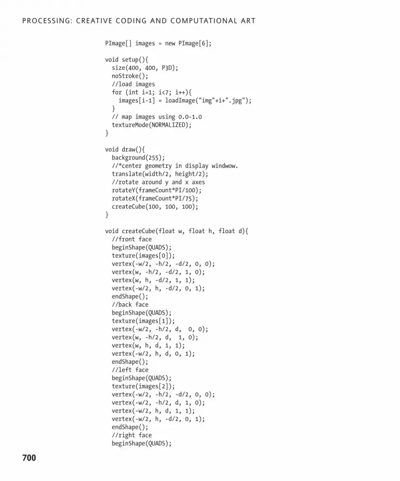
PImage[] images = new PImage[6];
void setup(){size(400, 400, P3D);noStroke();//load imagesfor (int i=1; i<7; i++){images[i-1] = loadImage("img"+i+".jpg");
}// map images using 0.0-1.0textureMode(NORMALIZED);
}
void draw(){background(255);//*center geometry in display windwow.translate(width/2, height/2);//rotate around y and x axesrotateY(frameCount*PI/100);rotateX(frameCount*PI/75); createCube(100, 100, 100);
}
void createCube(float w, float h, float d){//front facebeginShape(QUADS);texture(images[0]);vertex(-w/2, -h/2, -d/2, 0, 0); vertex(w, -h/2, -d/2, 1, 0); vertex(w, h, -d/2, 1, 1); vertex(-w/2, h, -d/2, 0, 1); endShape();//back facebeginShape(QUADS);texture(images[1]);vertex(-w/2, -h/2, d, 0, 0);vertex(w, -h/2, d, 1, 0); vertex(w, h, d, 1, 1);vertex(-w/2, h, d, 0, 1);endShape();//left facebeginShape(QUADS); texture(images[2]);vertex(-w/2, -h/2, -d/2, 0, 0); vertex(-w/2, -h/2, d, 1, 0); vertex(-w/2, h, d, 1, 1); vertex(-w/2, h, -d/2, 0, 1); endShape();//right facebeginShape(QUADS);
PROCESSING: CREATIVE CODING AND COMPUTATIONAL ART
700
617xAppA.qxd 4/26/07 10:57 AM Page 700

texture(images[3]);vertex(w, -h/2, -d/2, 0, 0);vertex(w, -h/2, d, 1, 0);vertex(w, h, d, 1, 1);vertex(w, h, -d/2, 0, 1);endShape();//top facebeginShape(QUADS);texture(images[4]); vertex(-w/2, -h/2, -d/2, 0, 0);vertex(w, -h/2, -d/2, 1, 0);vertex(w, -h/2, d, 1, 1);vertex(-w/2, -h/2, d, 0, 1);endShape();//bottom facebeginShape(QUADS); texture(images[5]);vertex(-w/2, h, -d/2, 0, 0);vertex(w, h, -d/2, 1, 0);vertex(w, h, d, 1, 1);vertex(-w/2, h, d, 0, 1);endShape();
}
Figure A-8. ImageMap sketch
PROCESSING LANGUAGE API
701
A
617xAppA.qxd 4/26/07 10:57 AM Page 701

InputThis is another large section in the API, generally involved in receiving or inputting data.Some of these processes are relatively low level, like reading bytes. However, Processing,as you’ve probably come to expect by now, encapsulates and simplifies these processes.The Input section includes 22 functions and 9 system variables, divided into five categories.The categories are as follows:
Mouse
Keyboard
Files
Web
Time & Date
MouseThe Mouse section includes six properties and five functions, used to evaluate when,where, and how mouse input is received by your running sketch. Variables such as mouseXand mousePressed provide live information about the mouse state; mouseX provides thecurrent x position of the mouse and mousePressed returns true or false depending if themouse button is pressed. Often, you can use this data creatively—for example, in a draw-ing program that colors pixels as the mouse moves over them.
The mouse functions, such as mouseMoved() or mouseDragged(), put code within separatefunction blocks (between the curly braces), allowing other functions or commands to becalled when the mouse motion event is detected. Following is a mouseMoved() examplethat illustrates some of the interesting things you can do via mouse detection (seeFigure A-9). There are a bunch of significant concepts within this example, and in spite ofit being a bit dense, the sketch is a good base for other experiments. When the sketchloads, move your mouse over the rectangle.
/*Box SpringsIra Greenberg, November 13, 2005revised October 11, 2006move mouse over white rectangle*/
// you can change block countint blocks = 40;float margin = 50;float boxHeight = 75;
PROCESSING: CREATIVE CODING AND COMPUTATIONAL ART
702
617xAppA.qxd 4/26/07 10:57 AM Page 702

//lots of arraysfloat[]x = new float[blocks];float[]y = new float[blocks];float[]w = new float[blocks];float[]h = new float[blocks];float[]py1 = new float[blocks];float[]py2 = new float[blocks];float[]radius = new float[blocks];float[]amplitude = new float[blocks];float[]frequency = new float[blocks];float[]ang = new float[blocks];float[]drag = new float[blocks];float[]gravity = new float[blocks];boolean[]isOver = new boolean[blocks];
void setup(){size(400, 300);background(0);noStroke();frameRate(30);/* amplitude, gravity, and frequencycan be messed with. Also, if you removethe random functions, you can get more standard wave patterns*/for (int i=0; i<blocks; i++){w[i] = (width-margin)/blocks;h[i] = boxHeight;x[i] = margin/2+w[i]*i;y[i] = height/2-h[i]/2;
amplitude[i] = random(20)+height/4;radius[i] = amplitude[i];gravity[i] = .85+random(.13);drag[i] = gravity[i];drawBlocks(x[i], y[i], w[i], h[i]);frequency[i] = 12+random(-5, 5);//flags let us know which box//we’re overisOver[i] = false;
}}
PROCESSING LANGUAGE API
703
A
617xAppA.qxd 4/26/07 10:57 AM Page 703

//main loopvoid draw(){fill(0, 50);rect(0, 0, width, height);fill(255, 255, 0);for (int i=0; i<blocks; i++){//you can add/subtract py1, py2 to x//and width arguments as welldrawBlocks(x[i], y[i]-py1[i], w[i], h[i]+py2[i]);// flags set in mouseMoved functionif (isOver[i]){//trig controls spring effectpy1[i] = sin(radians(ang[i]))*radius[i];py2[i] = cos(radians(ang[i]))*radius[i];// spring values affect color shiftfill(255, 255-radius[i], radius[i]*2);ang[i]+=frequency[i];radius[i]*=drag[i];
}}
}
/*While mosue is moving, detect whatbox the mouse is over and change flag.Also, need to reset radius, which isdecremented by drag - causing blocks to stop */void mouseMoved(){for (int i=0; i<blocks; i++){if (mouseX>x[i] && mouseX<x[i]+w[i] &&mouseY>y[i] && mouseY<y[i]+h[i]){radius[i] = amplitude[i];isOver[i] = true;
}}
}
//function to draw rectangles, called initially by//setup and then repeatedly in draw loopvoid drawBlocks(float x, float y, float w, float h){rect(x, y, w, h);
}
PROCESSING: CREATIVE CODING AND COMPUTATIONAL ART
704
617xAppA.qxd 4/26/07 10:57 AM Page 704

Figure A-9. Box Springs sketch
KeyboardThe Keyboard section is similar to the Mouse section in that it combines both system vari-ables and functions that allow you to communicate with the keyboard. The differencebetween the mouse and the keyboard is the amount and type of data input and output.The mouse can have multiple buttons, like a small keyboard, but it also has coordinatedata. The keyboard (at least mine) remains stationary, but has to translate between manypossible input values, for all the letters, numbers, and special keys that it uses. The keys onyour keyboard have integer values associated with them, commonly referred to as ASCIIcode. For example, the a key equals 65. There are also constant values for the special keys,such as UP, DOWN, LEFT, RIGHT, ALT/OPTION, CONTROL, SHIFT, BACKSPACE, TAB, ENTER, RETURN,ESC, and DELETE. The following simple example allows you to control a rectangle with thearrow keys. Notice in the code the use of the if (key == CODED) { } structure around thespecific key detection code.
int x, y;void setup(){size(200, 200);
}void draw() {stroke(0, 50);fill(255, 50);rect(width/2+x, height/2+y, 4+x, 4+y);
}void keyPressed() {
PROCESSING LANGUAGE API
705
A
617xAppA.qxd 4/26/07 10:57 AM Page 705

if(key == CODED) {if (keyCode == UP) {y--;
} else if (keyCode == DOWN) {y++;
} else if (keyCode == LEFT) {x--;
} else if (keyCode == RIGHT) {x++;
}}
}
FilesThe Files section includes four functions:
•openStream()
•open()
•loadStrings()
•loadBytes()
loadStrings() and loadBytes() allow you to load the contents of a file or URL as a stringarray or byte array, respectively. A byte array of a text file will include all the individualcharacters converted into their ASCII equivalents. If only a file name is specified as anargument with either of these functions, the file needs to reside within the sketch’s datadirectory. It’s also possible to specify a URL, assuming you use a valid path. Relative pathsshould be specified in relation to the data directory in the current sketch directory. Forexample, if your file (file.txt) is outside the data directory, in another directory calleddocs (also located within the sketch (parent) directory), it can be accessed (using UNIX/OSX path syntax) as: ../docs/file.txt, or on Windows: ..\docs\file.txt. The double dotsyntax (..) refers to the parent directory; (single dot syntax(.) refers to the current direc-tory). There is some general information about paths at http://en.wikipedia.org/wiki/Path_(computing).
The openStream() function provides a simplified way of using Java’s InputStream class.The InputStream class provides you with more control when inputting data. To learn moreabout Java’s InputStream class, check out http://java.sun.com/j2se/1.4.2/docs/api/java/io/InputStream.html.
Here’s what the Processing reference says about the open() function: “Attempts to open afile or process using the platform’s shell.” A shell is just an interface to your operating sys-tem. There are GUI (graphical user interface) shells, such as the Finder (OS X) or WindowsExplorer, where you simply click to launch an application. There are also command-lineshells, which is the type of shell the Processing reference is referring to. To communicatewith your system via a command-line shell, you type text-based commands in a terminal(emulator) program, such as the Terminal application in OS X. (On Windows, you canaccess the command shell by selecting the Run command in the Start menu and then
PROCESSING: CREATIVE CODING AND COMPUTATIONAL ART
706
617xAppA.qxd 4/26/07 10:57 AM Page 706

entering CMD). When using a command-line shell instead of a GUI shell, you need to beexplicit when issuing commands. It is common for modern GUI shells to hide the suffixesof files. In OS X, to launch the Calculator application using the Finder (GUI shell), youdouble-click the calculator icon, named simply “Calculator.” In contrast, from the Terminalapplication (command-line shell), you need to type: open Calculator.app. In addition, youneed to be explicit as to where files reside (the path) to access/launch them. When usingrelative paths with Processing’s open() command, you need to provide path addresses inrelation to the Processing application. For example, the Processing application on my com-puter lives within a Processing directory, which lives in the Applications directory. TheCalculator application also lives within the Applications directory. To launch theCalculator on a mouse press, I can use the following Processing sketch:
void draw(){}
void mousePressed(){open("../Calculator.app");
}
The open() command also allows to you pass a String argument. You can read moreabout open() at http://processing.org/reference/open_.html.
WebThe Web section includes the functions link(), param(), and status(). Stating the obvi-ous, these functions involve web-based features and are used within a browser environ-ment. link() allows you to load a web page, as well as specify which browser window touse (the existing one or a new one). param() reads the value of a parameter, specifiedwithin the HTML of a web page. For example, if you have the following HTML in the pageholding an applet, created from a sketch named SimpleBall:
<applet code="SimpleBall" archive=" SimpleBall jar"><param name="ballradius" value="50"> </applet>
you can use the param value ballradius in your SimpleBall sketch:
// SimpleBall sketchString strgRadius = param("ballradius");int radius = Integer.parseInt(strgRadius);size(200, 200);ellipse(width/2, height/2, radius, radius);
You’ll notice that the param value comes back as a String, so it needs to be converted toa number. Integer.parseInt() is a static method of Java’s Integer class that convertsstrings to integers. (Remember, in Processing, you can use Java code along with Processingcode.)
status() allows you to display messages in the browser’s status area—normally in thelower-left corner of the browser.
PROCESSING LANGUAGE API
707
A
617xAppA.qxd 4/26/07 10:57 AM Page 707

Time & DateTime & Date is the last subsection of the Input section of the API. The functions second(),minute(), hour(), day(), month(), and year() return a component of the time, based offyour system clock. The function millis() tells you how long, in milliseconds (thousandthsof a second), your sketch has been running since you started it. Here’s an analog clockexample (see Figure A-10):
/* Analog ClockIra Greenberg, October 9, 2006 */
PFont font;float x, y, r = 100;float textH = 12;
void setup(){size(400, 400);font = createFont("Arial", textH);textFont(font);x = width/2;y = height/2;smooth();
}
void draw(){background(75);drawClock();
}
void drawClock(){float px, py, angle = -60;fill(200);strokeWeight(4);ellipse(x, y, r*2, r*2);for (int i=1; i<13; i++){px = x+cos(radians(angle))*(r*.8);py = y+sin(radians(angle))*(r*.8);fill(0);// need to subtract 1/2 text width/height// to align centerfloat textW = textWidth(str(i));text(i, px-textW/2, py+textH/2);angle+=360/12;
}/*Subtract 90 degs. from each trig function, since 12is at top of clock (not at 0 postion on unit circle).Other numeric value is calculated by 360/number of units.*/
PROCESSING: CREATIVE CODING AND COMPUTATIONAL ART
708
617xAppA.qxd 4/26/07 10:57 AM Page 708
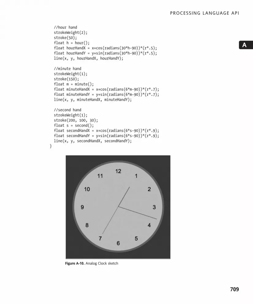
//hour handstrokeWeight(2);stroke(50);float h = hour();float hourHandX = x+cos(radians(30*h-90))*(r*.5);float hourHandY = y+sin(radians(30*h-90))*(r*.5);line(x, y, hourHandX, hourHandY);
//minute handstrokeWeight(1);stroke(150);float m = minute();float minuteHandX = x+cos(radians(6*m-90))*(r*.7);float minuteHandY = y+sin(radians(6*m-90))*(r*.7);line(x, y, minuteHandX, minuteHandY);
//second handstrokeWeight(1);stroke(200, 100, 30);float s = second();float secondHandX = x+cos(radians(6*s-90))*(r*.9);float secondHandY = y+sin(radians(6*s-90))*(r*.9);line(x, y, secondHandX, secondHandY);
}
Figure A-10. Analog Clock sketch
PROCESSING LANGUAGE API
709
A
617xAppA.qxd 4/26/07 10:57 AM Page 709

OutputThis section involves outputting data, both to the screen and to a file. As in the Input sec-tion, Processing makes these relatively low-level processes really easy to perform. Thissection is divided into three subsections:
Text Area
Image
Files
Text AreaText Area is a simple category that includes the two functions print() and println(). Bothoutput to the text area in the Processing window, but println() adds line returnsbetween each call to the function. You can use the string concatenator + within the argu-ment string, passed to the print() or println() function. For example, the followingcode outputs I love Processing:
String name = "Processing";print("I love "+name);
ImageImage includes two very cool functions that allow you to save screen image data to thesketch directory. saveFrame() will actually save a sequence of images in TIF, TGA, JPG, orPNG format. You can then import these sequenced images into video editing software andproduce movies of your Processing animations. save() just saves the current screenimage. Please note that neither of these functions will work when running your sketchesfrom within a web browser. This is a limitation of Java applets in general, imposed by Sunto “keep applets from compromising system security,” as mentioned in the article “WhatApplets Can and Can’t Do” (see http://java.sun.com/docs/books/tutorial/deployment/applet/security.html). To learn more about Java applets, check out http://java.sun.com/docs/books/tutorial/deployment/applet/index.html.
FilesThe Files subsection of the Output section is similar to the Files subsection of Input, exceptthings work in reverse. The two functions saveStrings() and saveBytes()—as you mightguess—save strings and bytes, respectively, to files within the current sketch directory.There are also two more general-purpose output functions, beginRecord() andendRecord(), which can be used to write out drawing functions as well as the contents ofthe display window (just be sure to call beginRecord() before the drawing calls you wantrecorded). To use these functions, you need to explicitly specify a renderer and file nameas arguments in the beginRecord(renderer, filename) call.
PROCESSING: CREATIVE CODING AND COMPUTATIONAL ART
710
617xAppA.qxd 4/26/07 10:57 AM Page 710

In the next example, I use beginRecord() and endRecord() as part of a simple drawingprogram (see Figure A-11). When you want to output your drawing, simply press any keyon the keyboard; this will cause your sketch to close and your drawing to be saved to yoursketch directory in PDF format.
/*Hairy Brush DrawingIra Greenberg, October 9, 2006outputs to PDF*/
import processing.pdf.*;
void setup() {size(400, 400);background(255);smooth();String id = str(hour())+"_"+str(minute())+"_"+str(second());beginRecord(PDF, "img"+id+".pdf");
}
void draw() {stroke(0);strokeWeight(4);if (mousePressed){line(pmouseX, pmouseY, mouseX, mouseY);bleed(pmouseX, pmouseY);
}}
void bleed(float x, float y){float px = 0, py = 0, angle = 0, radius=10;float brushDetail = 36;stroke(0, 100);strokeWeight(.5);for (int i=0; i<brushDetail; i++){px = x+cos(radians(angle))*random(radius);py = y+sin(radians(angle))*random(radius);line(x, y, px, py);angle+=360/brushDetail;
}}
// press any key on the keyboard to// output a pdf of your drawingvoid keyPressed() {endRecord();exit();
}
PROCESSING LANGUAGE API
711
A
617xAppA.qxd 4/26/07 10:57 AM Page 711

Notice the following statement at the top of the example:
import processing.pdf.*;
This imports Processing’s PDF library, one of Processing’s core libraries. Finally, note thatthe file functions will not work from a web browser.
Figure A-11. Hairy Brush Drawing sketch
TransformThis is a very cool part of the API, and one of the feature sets that makes Processing a trulyunique and powerful creative tool. However, all this coolness does come at a small price.The transform functions are a little complex and take some time to get your head around.While beginning to use them isn’t all that difficult, using them well can be a challenge. Atthe core of these functions is a mysterious mathematical structure called a matrix. Amatrix is just a table-like structure for organizing values. Matrices (plural) are central tolinear algebra (which I’m not going to go into), and they’re also central to computergraphics. What makes them so significant is the ease with which geometric transformationscan be done by using them.
PROCESSING: CREATIVE CODING AND COMPUTATIONAL ART
712
617xAppA.qxd 4/26/07 10:57 AM Page 712

Transformations include moving, scaling, skewing, and rotating vertices. Remember, ver-tices (points) are the foundation for all the other geometry you see on the screen. Thesimplest way to show how the transform functions work is through some examples. First,I’ll give you a (rather dull) example that transforms 2D geometry (see Figure A-12). ThenI’ll apply the concepts from the 2D example to a more interesting (albeit more compli-cated) 3D example.
//Example 1:noStroke();rect(10, 10, 25, 25);printMatrix();
pushMatrix();translate(20, 20);scale (1.5);rect(10, 10, 25, 25);printMatrix();popMatrix();
pushMatrix();translate(70, 70);scale (.5);rect(10, 10, 25, 25);printMatrix();popMatrix();printMatrix();
Figure A-12. Transform Example 1 sketch
PROCESSING LANGUAGE API
713
A
617xAppA.qxd 4/26/07 10:57 AM Page 713
This example isn’t too exciting, but it does illustrate the power and simplicity of doingmatrix transformations in Processing. In the example, I used the rect() command threetimes, using the same four arguments; yet I got three rectangles with different sizes andpositions. If you run this example, you should notice four tables of numbers output in theProcessing console. Each table is composed of two rows and three columns. These myste-rious numbers are the actual matrices at different states in the program. You’ll notice thatthe first and last table of numbers are identical:
1.0000 0.0000 0.00000.0000 1.0000 0.0000
These tables represent the base, or identity, matrix, without any transformation applied.The first rectangle I created used this matrix, before I called the first translate() func-tion, and that’s why what I input with regard to the arguments is what I got out. The othertwo rectangles have different transforms, and thus look different. In going over thissketch, you should take the time to see what parts of the matrix get changed after eachtransformation.
Another strange concept to deal with is the matrix stack. A stack is a temporary data struc-ture that operates following the last in, first out (LIFO) principal. Stacks are utilized inmany areas of computing, including managing transformation matrices. The pushMatrix()and popMatrix() functions alter the matrix stack, allowing different transformations tohappen in a seemingly independent fashion. When you want to create a localized trans-formation (not affecting everything following the transformation call), you first callpushMatrix(), which adds any transformations that follow it onto the matrix stack. Then,when you’re done, you call popMatrix(), which restores the matrix to its previous form.This is the reason that the first and last tables of values shown previously were identical—the first table represented the untransformed matrix and the last table represented thematrix after popMatrix() was called—which removed the last transformation pushed ontothe stack.
This next example (shown in Figure A-13) is much more interesting than the last, and reallyillustrates the power of this whole matrix business. But it’s also pretty complex and long;so watch it, play with it, and don’t worry about understanding all the code yet. After youget a sense of what the sketch does (visually), try messing with some of the values; it’s agreat way to see what’s going on programatically (and don’t worry about breaking thesketch, either). After you launch the example, let it run for a while, as there are somereally interesting patterns that form and change in interesting and unpredictable waysover time.
//Example 2:/*PushPopIra Greenberg, November 8, 2005*/
/*Need to import opengl library to use OPENGL rendering mode. You can also try runningin P3D mode*/import processing.opengl.*;
PROCESSING: CREATIVE CODING AND COMPUTATIONAL ART
714
617xAppA.qxd 4/26/07 10:57 AM Page 714

float ang;int rows = 20;int cols = 20;int cubeCount = rows*cols;int colSpan, rowSpan;float rotspd = 4;Cube[]cubes = new Cube[cubeCount];float[]angs = new float[cubeCount];float[]rotvals = new float[cubeCount];void setup(){size(400, 400, OPENGL);colSpan = width/(cols-1);rowSpan = height/(rows-1);noStroke();
// instantiate cubesfor (int i=0; i<cubeCount; i++){cubes[i] = new Cube(10, 10, 10, 0, 0, 0);/* 3 different rotation options- 1st option: cubes each rotate uniformly- 2nd option: cubes each rotate randomly- 3rd option: cube columns rotate as wavesTo try the different rotations, leave one of the rotVals[i] lines uncommented belowand the other 2 commented out.*/
//rotvals[i] = rotspd;//rotvals[i] = random(-rotspd*2, rotspd*2);rotvals[i]=rotspd+=.02;
}}
void draw(){int cubeCounter = 0;background(255);fill(200);//set up some different colored lightspointLight(51, 102, 255, width/3, height/2, 100); pointLight(200, 40, 60, width/1.5, height/2, -150);
//raise overall light in sceneambientLight(170, 170, 100);
//translate, rotate, and draw cubesfor (int i=0; i<cols; i++){for (int j=0; j<rows; j++){pushMatrix();/* translate each block.
PROCESSING LANGUAGE API
715
A
617xAppA.qxd 4/26/07 10:57 AM Page 715

pushmatrix and popmatrix add each cubetranslation to matrix, but restoreoriginal, so each cube rotates around itsowns center*/translate(i*colSpan, j*rowSpan, -20);//rotate each cube around y- and x-axesrotateY(radians(angs[cubeCounter]));rotateX(radians(angs[cubeCounter]));cubes[cubeCounter].drawCube();popMatrix();cubeCounter++;
}}//angs used in rotate function calls abovefor (int i=0; i<cubeCount;i++){angs[i] += rotvals[i];
}}
//simple Cube class, based on Quadsclass Cube {
//propertiesint w, h, d;int shiftX, shiftY, shiftZ;
//constructorCube(int w, int h, int d, int shiftX, int shiftY, int shiftZ){this.w = w;this.h = h;this.d = d;this.shiftX = shiftX;this.shiftY = shiftY;this.shiftZ = shiftZ;
}
/*main cube drawing method, which looks more confusing than it really is. It's just a bunch of rectangles drawn for each cube face*/void drawCube(){//front facebeginShape(QUADS);
PROCESSING: CREATIVE CODING AND COMPUTATIONAL ART
716
617xAppA.qxd 4/26/07 10:57 AM Page 716

vertex(-w/2 + shiftX, -h/2 + shiftY, -d/2 + shiftZ); vertex(w + shiftX, -h/2 + shiftY, -d/2 + shiftZ); vertex(w + shiftX, h + shiftY, -d/2 + shiftZ); vertex(-w/2 + shiftX, h + shiftY, -d/2 + shiftZ); endShape();//back facebeginShape(QUADS);vertex(-w/2 + shiftX, -h/2 + shiftY, d + shiftZ);vertex(w + shiftX, -h/2 + shiftY, d + shiftZ); vertex(w + shiftX, h + shiftY, d + shiftZ); vertex(-w/2 + shiftX, h + shiftY, d + shiftZ);endShape();//left facebeginShape(QUADS); vertex(-w/2 + shiftX, -h/2 + shiftY, -d/2 + shiftZ); vertex(-w/2 + shiftX, -h/2 + shiftY, d + shiftZ);vertex(-w/2 + shiftX, h + shiftY, d + shiftZ); vertex(-w/2 + shiftX, h + shiftY, -d/2 + shiftZ); endShape();//right facebeginShape(QUADS); vertex(w + shiftX, -h/2 + shiftY, -d/2 + shiftZ); vertex(w + shiftX, -h/2 + shiftY, d + shiftZ); vertex(w + shiftX, h + shiftY, d + shiftZ); vertex(w + shiftX, h + shiftY, -d/2 + shiftZ); endShape();//top facebeginShape(QUADS);vertex(-w/2 + shiftX, -h/2 + shiftY, -d/2 + shiftZ); vertex(w + shiftX, -h/2 + shiftY, -d/2 + shiftZ); vertex(w + shiftX, -h/2 + shiftY, d + shiftZ); vertex(-w/2 + shiftX, -h/2 + shiftY, d + shiftZ);endShape();//bottom facebeginShape(QUADS); vertex(-w/2 + shiftX, h + shiftY, -d/2 + shiftZ); vertex(w + shiftX, h + shiftY, -d/2 + shiftZ); vertex(w + shiftX, h + shiftY, d + shiftZ); vertex(-w/2 + shiftX, h + shiftY, d + shiftZ); endShape();
}}
PROCESSING LANGUAGE API
717
A
617xAppA.qxd 4/26/07 10:57 AM Page 717

Figure A-13. Transform Example 2 sketch
Lights, CameraThis is a very cool part of the API, but it is also pretty complex. Using the near 30 functionsin this section isn’t all that difficult, but understanding what’s happening underneath thesurface, and ultimately being able to control stuff, is the complex part. There are manysophisticated concepts built into a 3D renderer, including a virtual camera, light models,surface/material properties, and matrix transformations, just to name a few. I taught 3Dmodeling and animation for a number of years prior to delving into the programmatic sideof 3D, and I still find this stuff complicated and very challenging. If you are totally newto 3D (besides experimenting with Processing’s functions), I also recommend exploringsome 3D modeling and animation tools, such as LightWave, Maya, 3ds Max, or CINEMA 4D.
The Lights, Camera section is divided into four subsections:
Lights
Camera
Coordinates
Material Properties
PROCESSING: CREATIVE CODING AND COMPUTATIONAL ART
718
617xAppA.qxd 4/26/07 10:57 AM Page 718

LightsThe Lights section includes functions for controlling subtle, yet very important, aspects of3D rendering. In general, lighting in 3D is modeled on the real world and the concept ofplacing real lights in a space. The virtual camera is a similar such construct. Of course, inProcessing, all the lights are virtual, and really just a bunch of pixel color calculations. Thatbeing said, just as in the real world, virtual lights can have direction, falloff (how far andintensely they illuminate), color, cone angles (in the case of spotlights), and overall spatialillumination (in the case of ambient light). Lighting is one of the key research areas in 3D,and has an enormous impact on the overall quality of rendering.
CameraCamera functions control the virtual camera that you view the virtual world through. Thismight sound like an odd concept if you haven’t played with any 3D applications. A “real”3D projection is impossible on a flat 2D monitor, so ultimately all the 3D spatial calcula-tions need to be converted, or projected, back to the 2D Cartesian system. This translationis one of the aspects that makes 3D complicated. During this geometric flattening (whichusually happens in real time), different algorithms can be applied that control how weview the implied 3D space. For example, one of the most common approaches is to try tosimulate the effects of perspective, similar to how we, with our binocular vision, experi-ence the real world.
Based on the rules of perspective, objects get smaller as they go back in space, and in aone-point perspective system, lines going into the distance converge. When objects getclose to us and appear very large, distortions such as a fish-eye effect can occur. We caneasily simulate these types of effects in 3D—that is, with a lot of math. Conversely, we canalso create a more synthetic, or orthogonal, projection, in which there is no perspective.This is quite useful for precisely modeling geometry, where you might need to work with aset of undistorted 2D projections—for example, in an engineering application. Perspectivelooks good, but it is often hard to know precisely where you are (actually, where the cur-sor is) when working in this mode.
Virtual cameras also utilize a viewing volume and clipping planes that specify minimumand maximum values for the x-, y-, and z-axes. Normally, only stuff within the camera’sviewing volume, called the frustum, can be seen. The boundaries of the frustum are calledthe clipping planes. If the clipping planes are not set correctly, imagery can disappear andappear unexpectedly. However, without any clipping, geometry not visible within the cam-era’s view can get rendered, which is obviously a waste of memory. Finally, as the virtualcamera is not bound by the physics of the real world, it has the ability to produce highlydistorted and strange effects. This can be an interesting thing to experiment with, but alsoa potential source of frustration—especially when you don’t want it to happen (or can’ttrack down the problem).
CoordinatesThe Coordinates section includes six (conceptually) advanced functions that return coordi-nate values. The six functions are modelZ(), modelX(), modelY(), screenZ(), screenX(),
PROCESSING LANGUAGE API
719
A
617xAppA.qxd 4/26/07 10:57 AM Page 719

and screenY(). The model functions return the 3D coordinates in model space, whichmeans the coordinate values after they’ve been transformed (rotated, scaled, and/ormoved), but before they’re projected to the screen. In contrast, the screen functionsreturn 3D coordinates in relation to screen space. If you’ve never worked in 3D, this maysound pretty confusing. Remember, computer-generated 3D simulates space, as every-thing really lives on the 2D screen surface. To simulate real space, geometry must beshifted around to give the illusion of perspective, depth layering, and so forth. The actual3D coordinate geometry we generate ultimately has to be mapped to the space of our 2Dscreens, taking into account any perspective calculations. This concept is most abstract inreference to the z-axis, which doesn’t really exist at all on the screen. Yet, when we workin 3D, geometry is calculated at specific locations on this illusory axis. To visualize the con-cept of screen coordinates vs. model coordinates, think about the classic one-point per-spective image of railroad tracks receding into the distance to a point. In reality, of course,the tracks remain parallel and never actually converge—which you can think of as theirmodel coordinates (the actual geometry). But visually, the receding tracks are no longerparallel, and these illusory coordinates can be thought of as their screen coordinates.
Material PropertiesThe Material Properties section includes four functions:
shininess()
specular()
ambient()
emissive()
These functions control how object surfaces interact with the light in the scene. For exam-ple, glossy and reflective surfaces have concentrated areas of light, sometimes referred toas hotspots; think about the small, intense light spots on the surface of an eyeball, or howlight reflects off of a highly polished piece of chrome. This light phenomenon is referredto as specularity. The specular() function controls the color of these hotspots.
Ambient light, on the other hand, refers to more general and overall lighting—think aboutthe light in a dense forest or in a room without a direct light source. The ambient() func-tion controls the color of the ambient light. Like the other rendering attribute functions,the material functions affect the rendering state as well as the light functions. Once amaterial function (e.g., shininess()) is called, its influence will be felt by all future sur-faces created in the scene, until another explicit call to the material function (using differ-ent rendering attributes) is made.
To give an example that involves the Lights, Camera section of the API, I developed a 3Dflythrough sketch that utilizes a lot of the features I’ve been discussing. (This is anothercomplex sketch that I put in more for inspiration and pleasure than your edification—butit is cool, and will still be useful for you to take apart and experiment with.)
The example (shown in Figure A-14) utilizes two images that need to be put within thesketch’s data directory. The images need to be named ground2.jpg and metal2.jpg, and Irecommend making them around 400 by 400 pixels. If the example runs slowly on your
PROCESSING: CREATIVE CODING AND COMPUTATIONAL ART
720
617xAppA.qxd 4/26/07 10:57 AM Page 720

system, you can try lowering the resolution of the images (in an image editing program),lowering the value of the bldgCount variable in the sketch, or buying yourself a new com-puter. If you go with option 3, I’ll take a new Mac laptop while you’re at it.
/*FlyThroughIra Greenberg, November 8, 2005*/
/*Need to import opengl library to use OPENGL rendering mode. You can also try runningin P3D mode*/import processing.opengl.*;
// images used for mappingPImage ground, brick;
// camera move variablesfloat bank=2;float bankAngle;float bankSpeed = .7;float vert = -600;float zoom;float vertSpeed = 1.5;float heading;float headingSpeed = -.75;float pitch;float pan;float zoomSpeed = 1.6;
//structuresint bldgCount = 300;BLDG[]bldgs = new BLDG[bldgCount];BLDG plane;
void setup(){size(600, 400, OPENGL);noStroke();textureMode(NORMALIZED);
//load image mapsground = loadImage("ground2.jpg");brick = loadImage("metal2.jpg");
//set up ground planeplane = new BLDG(width*10, 0, width*10, 0, 60, 0, ground);
// instantiate bldgsfor (int i=0; i<bldgCount; i++){
PROCESSING LANGUAGE API
721
A
617xAppA.qxd 4/26/07 10:57 AM Page 721

bldgs[i] = new BLDG(10+random(30), random(100, 840), 10+random(50),random(-width*2, width*2), 60, random(-width*3, width*2), brick);
}}
void draw(){background(4, 4, 20);// set camera and lightscamera(width/2.0+pan, height/2+vert, ((height/2.0+1500-zoom) / tan(PI*60 / 360.0)), width/2.0+pan, height/2+vert, -8000, 0, 1, 0);fill(200);//set up some different colored lightsambientLight(90, 65, 52); pointLight(51, 102, 255, width/3, height/2, 100); pointLight(200, 40, 60, width/1.5, height/2, -150);pointLight(20, 220, 25, -200, -100, 300);pointLight(110, 55, 40, width*4, height/2, 1000);
//draw ground planepushMatrix();translate(width/2, height/2, -20);rotateY(radians(heading));rotateX(radians(pitch));rotateZ(radians(bank));plane.drawBLDG();// draw buildingsfor (int i=0; i<bldgCount; i++){bldgs[i].drawBLDG();
}popMatrix();
//moonspotLight(255, 255, 10, 80, -300, -400, -1, 0, 0, PI/1.4, 2);pushMatrix();translate(-600, -1500, -100);fill(75, 185, 40, 255);sphere(75);popMatrix();
//planetpointLight(20, 220, 25, 2000, -4000, -2000);pushMatrix();translate(2500, -4700, -2200);fill(100, 100, 180, 55);sphere(3200);popMatrix();
//camera movesbank = sin(radians(bankAngle))*12;
PROCESSING: CREATIVE CODING AND COMPUTATIONAL ART
722
617xAppA.qxd 4/26/07 10:57 AM Page 722

bankAngle+=bankSpeed;vert = -600 +zoom*.24;zoom+=zoomSpeed;if (zoom>2200 || zoom<-10) {zoomSpeed*=-1;
}heading+=headingSpeed;
}//simple BLDG classclass BLDG {//propertiesfloat w, h, d;float shiftX, shiftY, shiftZ;PImage img;
//constructorBLDG(float w, float h, float d, float shiftX,float shiftY, float shiftZ, PImage img){this.w = w;this.h = h;this.d = d;this.shiftX = shiftX;this.shiftY = shiftY;this.shiftZ = shiftZ;this.img = img;
}
//main bldg drawing methodvoid drawBLDG(){beginShape(QUADS);texture(img);//front wallvertex(-w/2 + shiftX, -h/2 + shiftY, -d/2 + shiftZ, 0, 0);vertex(w + shiftX, -h/2 + shiftY, -d/2 + shiftZ, 1, 0); vertex(w + shiftX, shiftY, -d/2 + shiftZ, 1, 1); vertex(-w/2 + shiftX, shiftY, -d/2 + shiftZ, 0, 1);
//back wallvertex(-w/2 + shiftX, -h/2 + shiftY, d + shiftZ, 0, 0); vertex(w + shiftX, -h/2 + shiftY, d + shiftZ, 1, 0); vertex(w + shiftX, shiftY, d + shiftZ, 1, 1);vertex(-w/2 + shiftX, shiftY, d + shiftZ, 0, 1);
//left wallvertex(-w/2 + shiftX, -h/2 + shiftY, -d/2 + shiftZ, 0, 0);vertex(-w/2 + shiftX, -h/2 + shiftY, d + shiftZ, 1, 0); vertex(-w/2 + shiftX, shiftY, d + shiftZ, 1, 1);vertex(-w/2 + shiftX, shiftY, -d/2 + shiftZ, 0, 1);
PROCESSING LANGUAGE API
723
A
617xAppA.qxd 4/26/07 10:57 AM Page 723

//right wallvertex(w + shiftX, -h/2 + shiftY, -d/2 + shiftZ, 0, 0); vertex(w + shiftX, -h/2 + shiftY, d + shiftZ, 1, 0); vertex(w + shiftX, shiftY, d + shiftZ, 1, 1); vertex(w + shiftX, shiftY, -d/2 + shiftZ, 0, 1);
//roofvertex(-w/2 + shiftX, -h/2 + shiftY, -d/2 + shiftZ, 0, 0);vertex(w + shiftX, -h/2 + shiftY, -d/2 + shiftZ, 1, 0); vertex(w + shiftX, -h/2 + shiftY, d + shiftZ, 1, 1); vertex(-w/2 + shiftX, -h/2 + shiftY, d + shiftZ, 0, 1); endShape();
}}
Figure A-14. FlyThrough sketch
ColorThe Color section is divided into two subsections: Setting and Creating & Reading. Althoughit’s a relatively small section of the API, it’s a very significant one. For the most part, theColor section is pretty straightforward, with simple background(), fill(), and stroke()functions that take arguments to directly change color. However, there are two issues thatmay be new or challenging to newbie coders, which I’ll discuss in the following respectivesections.
PROCESSING: CREATIVE CODING AND COMPUTATIONAL ART
724
617xAppA.qxd 4/26/07 10:57 AM Page 724

SettingThe Setting section includes the basic functions just discussed. One issue that may be newto you is the concept of a rendering state or graphics context. Graphics application soft-ware can make it seem that color is generated on a per-shape basis. If you need a blue rec-tangle, you grab the paint bucket tool, select a blue color, and click in your shape (or somesimilar procedure). What a tool like the paint bucket conceals is how color is implementedas a state change in a programming language like Java and Processing. As a comparison,I’ve included the code for a simple Java graphics application followed by its Processingequivalent. Both programs generate the same output, except that the Java program does itin 19 lines (not including comments or skipped lines), while Processing does it in 5. Do nottry to run the Java application from within Processing; it will not work. (As an aside, for thefew experienced Java readers out there—and this comes from Ben Fry directly—classesfrom the java.awt.* and javax.swing.* packages should not be used within Processing,as they will generate inconsistent results.) What the Java vs. Processing code comparisonshould show you is how much stuff Processing handles under the hood, or encapsulates,making our coding lives happier. Here’s the Java version:
import java.awt.*;import java.applet.*;
public class SimpleJavaExample extends Frame {//constructor
public SimpleJavaExample(){setSize(200, 200);setBackground(Color.white);// this program still requires window closing behavior
}//main methodpublic static void main(String[]args){new SimpleJavaExample().setVisible(true);
}//overrides default paint methodpublic void paint(Graphics g){g.setColor(new Color(0, 0, 200));g.fillRect(25, 50, 50, 50);g.fillOval(125, 50, 50, 50);g.setColor(new Color(0, 0, 0));g.drawRect(25, 50, 50, 50);g.drawOval(125, 50, 50, 50);
}}
In Processing, to get the same output, you can just write the following:
size(200, 200);background(255);fill(0, 0, 200);rect(25, 25, 50, 50);ellipse(150, 50, 50, 50);
PROCESSING LANGUAGE API
725
A
617xAppA.qxd 4/26/07 10:57 AM Page 725

Color, rather than being generated on a per-object basis, is part of an overall renderingstate, or graphics context. In Processing and Java, this graphics context is controlled by aGraphics object, which sets properties of the rendering state, such as color and font, aswell as a few others. Graphics is the base class in Java that encapsulates this process,allowing you to write relatively simple code, as in the Java example. Processing, as you’dexpect, encapsulates this stuff even further, removing the need for explicitly overriding thepaint() method, as in the Java example. The paint() method is the method that a Javacomponent (a component can be thought of as a panel—like the display window) callswhen it needs to paint something. What I’m actually doing in the Java example is redefin-ing the paint() method for my component, so when paint() is called normally by thecomponent, which happens automatically when the program starts, it will use my paintmethod, instead of the component’s default one, to do what I want it to do—in this case,paint a simple blue rectangle and circle on the screen. This process of using one method’simplementation to replace another is referred to as method overriding, and is a funda-mental part of OOP.
If you run the Processing code, you’ll notice that the sketch includes two blue shapes. Thisis because the state of the rendering context hasn’t been changed between the two callsto the drawing functions. Thus, the fill is not really about those two shapes, but about thecurrent rendering state of the program at that point. Until you change the rendering statecolor with another fill() command call, every new filled shape will be blue. I’ll shut upabout this now, but if you want to learn more about the Java Graphics class from Sun,check out http://java.sun.com/j2se/1.4.2/docs/api/index.html. And here’s a link tosome more info about how painting works in Java: http://java.sun.com/products/jfc/tsc/articles/painting/.
The next sketch is another example of the Color section’s Setting functions in action (seeFigure A-15). One of the functions, colorMode(), deserves a little clarification. Color canbe specified as RGB (red, green, blue—the default mode) or HSB (hue, saturation, bright-ness). In addition, you can set the mathematical range to describe the color, or even eachpart of the color. In my two calls to colorMode() in the example, the first call,colorMode(RGB, 1.0), sets the mode to RGB and specifies the range of values to be set foreach component between 0.0 and 1.0. Thus, (0, 0, 0) would equal black, and (.5, .5, 0)would equal yellow. The second call is pretty odd, and I only did it as an extreme exampleof what is possible. colorMode(HSB, 100, 10, .1) sets the mode to HSB. It specifies thehue value range from 0 to 100 (which is what you typically see with HSB values—0 to 100percent), the saturation range from 0 to 10, and the brightness range from 0 to .1 (whichis pretty odd, indeed). However, it all works, and may even impress your friends (probablynot). Wikipedia has an interesting discussion on HSB (sometimes also referred to as HSV)at http://en.wikipedia.org/wiki/HSB_color_space.
/*Simple Color ExampleIra Greenberg, November 10, 2005 */size(200, 200);background(200, 50, 40);stroke(45);fill(200, 200, 0);rect(25, 50, 50, 50);
PROCESSING: CREATIVE CODING AND COMPUTATIONAL ART
726
617xAppA.qxd 4/26/07 10:57 AM Page 726

ellipseMode(CORNER);fill(200, 200, 0, 125);stroke(175, 0, 255);ellipse(125, 50, 50, 50);
noStroke();colorMode(RGB, 1.0);fill(0, .85, .2);triangle(25, 175, 75, 175, 50, 125);
colorMode(HSB, 100, 10, .1);fill(50, 9, .08);beginShape();vertex(125, 125);vertex(120, 145);vertex(140, 160);vertex(145, 170);vertex(175, 175);vertex(182, 150);vertex(155, 138);vertex(145, 120);endShape(CLOSE);
Figure A-15. Simple Color Example sketch
PROCESSING LANGUAGE API
727
A
617xAppA.qxd 4/26/07 10:57 AM Page 727

Creating & ReadingAs discussed previously, color is specified as three components, for red, green, and blue(RGB). (You can also specify a fourth component, alpha, for controlling transparency.)Most typically on the computer, color is referred to as a hexadecimal value. Thehexadecimal system uses 16 as the base, instead of 10, as in the more common decimalsystem. To account for 16 unique numbers, the letters A, B, C, D, E, and F are used alongwith the numbers 0 through 9. Also remember that 0 counts as a digit, so F is equal to 15,while B equals 11. Numbers larger than 15 are created by using additional places, just as inthe decimal system. However, the values are raised by 16 instead of 10. So, the number FFwould be equal to 15 * 16 + 15, which equals 255, and the number AFB would equal (10 *16 * 16) + (15 * 16) + 11, which equals 2,811. To allow the computer to know that youwant it to perform calculations using base 16 instead of base 10, you write 0x before thevalue. So, AFB would be specified as 0xAFB.
Try running this one-line sketch, which should output 2811:
println(0xAFB);
In Processing, you can also use also the # symbol to specify a color value, as in the follow-ing line:
color orange = #FF7700;
Each color is specified as a six-digit hexadecimal value, where the first two numbers spec-ify the red component, the next two the green, and the final two the blue. For example,the colors red, green, and blue are specified as #FF0000, #00FF00, and #0000FF. Of course,you can any put legal hexadecimal characters (0 through 9 and A through F) in any of thesix slots to create up to 16,777,215 different colors.
The seven functions red(), brightness(), blue(), saturation(), green(), hue(), andalpha() extract specific values out of a color. For example, if I want the blue componentof the color 0xFFE56D, I can use this simple code:
color c = 0xFFE56D;print(blue(c));
I can use the exact same structure for most of the functions within this section. Here’scode to extract the saturation of a color:
color c = 0xFFE56D;print(saturation(c));
Curiously, if you look at what the API has to say about the red() function, there’s a myste-rious blurb in the Description section: “The red() function is easy to use and understand,but is slower than another technique. To achieve the same results when working incolorMode(RGB, 255), but with greater speed, use the >> (right shift) operator with a bitmask” (see http://processing.org/reference/red_.html).
Right shift operator, bit mask—what is this stuff? Unfortunately, there’s not much else togo on in the API. It seems there may be some pretty scary stuff lurking beneath the surface
PROCESSING: CREATIVE CODING AND COMPUTATIONAL ART
728
617xAppA.qxd 4/26/07 10:57 AM Page 728

of this part of the API. These mysterious terms relate to bitwise operations. Bitwise opera-tions are low-level operations useful for squeezing some extra performance out of asketch, but they’re also a little (actually more than a little) confusing to use. I cover bitwiseoperations further in Appendix B.
Processing has a convenient data type called color that encapsulates the 32 bits of infor-mation making up a color (8 bits for alpha, 8 bits for red, 8 bits for green, and 8 bits forblue). You can declare a variable of type color using the following syntax:
color c
In the Image section of the API, which I’ll look at next, is a function named get(). get()returns a value as a color data type based on a specific pixel’s color. Another way to cre-ate a color from scratch is to use the color() function. (I realize it gets confusing when anumber of different commands/data types share common names). Finally, you can createa color by directly assigning a hexadecimal value to a color variable. Following are threestatements that generate a color three different ways: through the use of get(), throughthe use of the color() function, and through direct assignment using hexadecimal nota-tion. I also include a fourth direct assignment statement that includes an alpha componentin the hexadecimal notation.
color c1 = get(50, 50);color c2 = color(200, 100, 50);color c3 = #FF33DD;// this last statement explicitly specifies alpha and RGB valuescolor c4 = 0xFFFF33DD;
The Creating & Reading subsection also includes two color-blending functions:blendColor() and lerpColor(). blendColor(), the more complex of the two functions,utilizes a blending mode, declared as an argument passed to the function, along with thetwo colors to blend. lerpColor() uses a simpler numeric ratio for blending two colors.Here’s an example that uses both functions, including blendColor()’s different blendingmodes (see Figure A-16):
/* blendColor and lerpColorIra Greenberg, October 12, 2006 */
size(210, 490);background(100);noStroke();smooth();color c1 = color(200, 10, 200);color c2 = color(200, 200, 10);
//blendcolor c_add = blendColor(c1, c2, ADD);color c_subtract = blendColor(c1, c2, SUBTRACT);color c_darkest = blendColor(c1, c2, DARKEST);color c_lightest = blendColor(c1, c2, LIGHTEST);
PROCESSING LANGUAGE API
729
A
617xAppA.qxd 4/26/07 10:57 AM Page 729

//lerpcolor c_lerp_25 = lerpColor(c1, c2, .25);color c_lerp_5 = lerpColor(c1, c2, .5);color c_lerp_75 = lerpColor(c1, c2, .75);
color[] cols = {c_add, c_subtract, c_darkest, c_lightest, c_lerp_25, c_lerp_5, c_lerp_75
};
for (int i=0; i<cols.length; i++){fill(c1);ellipse(35, 35+70*i, 70, 70);fill(cols[i]);ellipse(105, 35+70*i, 70, 70);fill(c2);ellipse(175, 35+70*i, 70, 70);
}
Figure A-16. BlendColor and LerpColor sketch
PROCESSING: CREATIVE CODING AND COMPUTATIONAL ART
730
617xAppA.qxd 4/26/07 10:57 AM Page 730

ImageThe Image section relates very directly to the information I covered in the Color section, asan image after all is a just a collection of colored pixels. In general, the image functionsallow you to load and alter images. In Java, loading images and altering them is real work(especially down at the pixel level). Processing, as usual, simplifies this entire process, whilestill giving you enough low-level access to act directly upon the pixel data. Processing alsoincludes its own image data type, called PImage, that encapsulates many of the features,which makes working with images in Processing so easy. Yet, for all its ease of use,Processing’s imaging capabilities are surprisingly powerful.
The Image section of the API is divided up into essentially two categories, with the PImagedata type and createImage() function standing alone. The two categories are Loading &Displaying and Pixels. Be aware that PImage includes a bunch of methods with the samenames as some of the functions in the Pixels section. For instance, following is an examplethat uses the PImage method get() and the function get() in the same sketch. Eventhough these commands are both called get(), they are fundamentally different. Theget() method requires a PImage object to call it—as in myImage.get()—while the get()function works all by itself. The subtlety of this distinction requires an understanding ofOOP, which is covered in Chapter 8.
You’ll need an image named portrait.jpg in the data directory of this sketch to run thisexample. I suggest making the image 400 by 400 pixels.
size(400, 400);PImage img = loadImage("portrait.jpg");image(img, 0, 0);println("image method before = " + img.get(50, 50));println("function before = " + get(50, 50));image(img, -140, -140);println("image method after = " + img.get(50, 50));println("function after = " + get(50, 50));
Here’s the output generated by running the sketch:
image method before = -263171function before = -263171image method after = -263171function after = -5686717
Your values will be different, since your image will be different than mine—but notice howthe output changes for the function, but not for the method. What’s happening is that thePImage get() method references the image data stored in the PImage object independ-ently from its display on the screen, while the get() function returns pixel values at a spe-cific point on the screen. Since I drew the image at two different places on the screen, thetwo get() function calls give two different values. However, the two get() method callsrefer to the same pixel in the stored PImage object.
PROCESSING LANGUAGE API
731
A
617xAppA.qxd 4/26/07 10:57 AM Page 731

PixelsThe Pixels section includes functions that operate at the pixel level. In addition to func-tions that provide access to the entire pixel array of the display, there are two simple yetpowerful functions for blending and filtering image data that provide programmaticallycontrolled Photoshop-like capabilities. If you don’t want to use these cool included func-tions for doing things like blurs, posterization, image masking, and compositing, you caneasily spin your own, as well; just grab the image pixels using the loadPixels() function,do some bit shifting, and then just call updatePixels() to rewrite the pixel data to thescreen. In addition to using the get() function or the PImage get() method to access thecolor of a pixel, it is also possible (and faster) to access the pixels[] array directly. Similarto the two get() commands just discussed, there are two pixels[] arrays in Processing—one represents the contents of the display window and the other is a property within thePImage class. Similar to the get() method, this pixels[] array property requires a PImageobject to be accessed (e.g., myImage.pixels), and the array data only relates to the PImageobject, independent of the display window. Here’s an example that uses both get() com-mands and pixels[] arrays. This example also uses the portrait.jpg image, which shouldbe in the sketch’s data directory.
size(400, 400);//create a Pimage and load an external imagePImage img = loadImage("portrait.jpg");//PImage method get() works even without drawing image to the screenprintln("PImage get() method = " + img.get(50, 50));//PImage pixels[] array may also be accessed without drawing !
the image to the screenprintln("PImage pixel array = " + img.pixels[50*width+50]);//draw the image to the screenimage(img, 0, 0);// display window get() function works without calling loadPixels();println("get() function = " + get(50, 50));loadPixels();// loadPixels() must be called prior to accessing display window !
pixels[] array directlyprintln("pixel array = " + pixels[50*width+50]);
It is confusing that these two arrays have the same name but function differently. As Imentioned, you can access the pixel values of a PImage object directly, even prior to draw-ing the image to the screen, using object-oriented dot syntax, as in myImage.pixels.However, to access the pixel values of the display window, you must first callloadPixels(), as I did in the preceding example. With regard to the two get() com-mands, neither command requires loadPixels() to be called prior to being used. OnceloadImage() has been called, the PImage get() method can access pixel values within theimage. However, to access the image pixel value using the display window get() function,you need to draw the image to the screen using the image() command.
PROCESSING: CREATIVE CODING AND COMPUTATIONAL ART
732
617xAppA.qxd 4/26/07 10:57 AM Page 732

Loading & DisplayingThe Loading & Displaying section includes two functions that make working with images inProcessing a joy: loadImage() and image(). loadImage("imageName") expects a singleString argument, which should be the name of the file you want to load, residing in thesketch’s data directory. It is critical that you first load your image files into Processing byselecting Add File from the Sketch menu. When you select Add File, your loaded image willbe placed in a data subdirectory, within the current sketch main directory. If you don’talready have a data directory, it will be created for you. If you’ve successfully run the lastfew examples, you already know how to do this.
It is recommended that you do all your image loading in the setup() structure, not indraw(). After you load an image using loadImage(), you won’t see it until you render it tothe screen. This is another one of those things that’s not so simple to do in Java, butincredibly simple to achieve in Processing—just call image(). This function can take abunch of arguments, including a PImage object reference and the x, y, width, and heightproperties of the image.
This subsection also includes basic tinting functions and a simple utility function calledimageMode() that gives you two options for specifying image measurements in the displaywindow when you call the image() function. The default CORNER argument option allowsyou to specify x, y, width, and height properties, while the CORNERS argument makes thethird and fourth measurement arguments (that were width and height) specify the posi-tion of the bottom-right point of the image. In both cases, when passing arguments thatcontrol width and height, you can scale and load the images simultaneously. Be aware thatyou can scale the images both proportionally and non-proportionally based on the ratio ofyour arguments.
As an example, I created a simple progressive tiling sketch that loads an image, and thencontinuously shrinks the image as it tiles it through the display window (see Figure A-17).Be aware that there is the possibility of generating an infinite loop with this example—oneof Zeno’s paradoxes, in which a float value keeps approaching a discrete value, but neverreaches it. You can read about Zeno’s paradoxes at http://en.wikipedia.org/wiki/Zeno%27s_paradox. If you test this, please remember to first add your image file into thedata directory using the Add File command. (This sketch uses the image vail.jpg.)
/*Progressive TileIra Greenberg, November 12, 2005*/
size(480, 480);background(255);PImage img = loadImage("vail.jpg");float x = 0, y =0;float w = 240*.5;float h = w;for (int i=0; i<height; i+=h){for (int j=0; j<width; j+=w){image(img, j, i, w, h);
PROCESSING LANGUAGE API
733
A
617xAppA.qxd 4/26/07 10:57 AM Page 733

}// avoid infinite loop// Zeno's paradox waiting to happenif (w>5){w*=.81;h*=.81;
}}
Figure A-17. Progressive Tile sketch
RenderingThis section includes the PGraphics data type and the createGraphics() function.Together, these elements provide low-level access into Processing’s graphics and renderingcontext—sort of the meat (or tempeh, for vegan readers) and potatoes of the ProcessingAPI. PGraphics is one of Processing’s core, base classes, and it has a rich set of propertiesand methods, which you can learn more about at http://dev.processing.org/reference/core/javadoc/processing/core/PGraphics.html. One of the main uses for
PROCESSING: CREATIVE CODING AND COMPUTATIONAL ART
734
617xAppA.qxd 4/26/07 10:57 AM Page 734

these elements is the creation of an off-screen image, also sometimes referred to as animage buffer. Beyond drawing to the display window, you can also use thecreateGraphics() function to generate a PGraphics object that you can draw directlyinto. You can then output this off-screen image to the screen, or even save it to a file.
The next example uses these two structures to generate an off-screen image that willeventually be turned into a tiled background (see Figure A-18). The sketch allows a user todraw within the display window. The drawing is simultaneously output to the screen (usingProcessing’s built-in graphics context) and written to an off-screen buffer (using aPGraphics object created with the createGraphics() function). When the user releasesthe mouse, the off-screen image is scaled, positioned, and drawn to the screen as a tiledfill pattern. Notice in the sketch code that the two PGraphics methods beginDraw() andendDraw() are used, in a sense, as entry and exit portals for drawing to the off-screenPGraphics object.
/* Tile DesignerIra Greenberg, October 11, 2006draw to off-screen bufferto create a tiled background */
PGraphics p;int tiles = 10;float strokeWt = 2.75;float scaleFactor;boolean isRecordable = false;
void setup() {size(400, 400);background(0);smooth();float tileWidth = width/tiles;scaleFactor = tileWidth/width;
}
void draw() {// write to off-screen bufferif (isRecordable){p.line(pmouseX, pmouseY, mouseX, mouseY);
}// preview drawing of tileif (mousePressed){stroke(255);line(pmouseX, pmouseY, mouseX, mouseY);
}}
void mousePressed(){p = createGraphics(width, height, JAVA2D);noStroke();
PROCESSING LANGUAGE API
735
A
617xAppA.qxd 4/26/07 10:57 AM Page 735
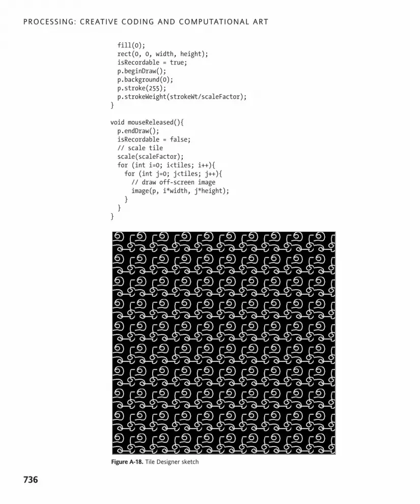
fill(0);rect(0, 0, width, height);isRecordable = true;p.beginDraw();p.background(0);p.stroke(255);p.strokeWeight(strokeWt/scaleFactor);
}
void mouseReleased(){p.endDraw();isRecordable = false;// scale tilescale(scaleFactor);for (int i=0; i<tiles; i++){for (int j=0; j<tiles; j++){// draw off-screen imageimage(p, i*width, j*height);
}}
}
Figure A-18. Tile Designer sketch
PROCESSING: CREATIVE CODING AND COMPUTATIONAL ART
736
617xAppA.qxd 4/26/07 10:57 AM Page 736

TypographyProcessing utilizes multiple approaches to rendering typography in your sketches, includ-ing both raster- and vector-based solutions. Historically for graphic designers, typographyon the Web has required a cost-benefit analysis between using common but ubiquitousfonts (i.e., native fonts, which are likely to be installed on most users’ systems) and usingmore involved, memory-intensive, or unpredictable solutions. Processing sketches arewidely distributed as applets on the Web, so there are some similar trade-offs when usingtypography in your sketches.
The Typography section is divided into four sections:
PFont
Loading & Displaying
Attributes
Metrics
PFontPFont is Processing’s custom font data type. When using type in Processing, you first needto declare a PFont object. This object is then assigned a reference to a specific font. Forexample, assuming you have a font named Verdana-24.vlw in the data directory of yourcurrent sketch, you can render type in Processing using the following:
PFont f = loadFont("Verdana-24.vlw"); textFont(f);text("Hello", 19, 55);
Processing’s VLW format is a custom bitmapped font format, which relies on a brute-forceapproach to incorporating typography into sketches—characters are described as images,rather than with a scalable vector format. The benefit of this arrangement is that fonts notinstalled on a user’s system can still be rendered in Processing, which would not be thecase if Processing depended only upon installed native fonts.
Although the VLW format solves the missing typeface problem, it is not without its ownchallenges. When a typeface is converted to the VLW format, it should be specified at theexact point size it will be rendered at or it may not render clearly. This means that if youuse the same font at varying sizes throughout your sketch, you’ll want to create a numberof separate VLW fonts for the different sizes (even though it’s the same font). Sketch per-formance is also negatively impacted when the VLW fonts are not created at the specifiedrendering sizes in your sketch.
Before you completely write off typography in Processing, you should note that it’s possi-ble to use vector-based typography in Processing as well. You can ask Processing to usenative (scalable vector) fonts, assuming the user has the specific font installed on their sys-tem, by including the following command in your sketch:
hint(ENABLE_NATIVE_FONTS);
PROCESSING LANGUAGE API
737
A
617xAppA.qxd 4/26/07 10:57 AM Page 737

Processing can also render TTF (TrueType) and OTF (OpenType) font vector formats, aslong as the font is installed in your sketch’s data directory. Thus, it is possible to distributeyour sketch on the Web or directly to another user with the specific TTF or OTF fontincluded in the sketch’s data directory. However, there are legal/copyright issues involvedin distributing fonts like this, as the Processing reference states: “Only fonts that can legallybe distributed should be included with a sketch” (see http://processing.org/reference/createFont_.html).
Finally, type in Processing can also be rendered in 3D space, although there is some qual-ity loss for this very cool capability. If quality is critical, use the textMode(SCREEN) com-mand, which forces the type rendering to the front of the display window, increasingrendering quality.
Loading & DisplayingThe Loading & Displaying subsection has four main functions that allow fonts to be dis-played in Processing, as follows (please note that the Processing language reference liststext() first, but I’ll discuss it last):
text()
createFont()
loadFont()
textFont()
createFont() dynamically converts a font installed on your computer to the VLW formatused by Processing. This function works similarly to the Create Font command in the Toolsmenu. However, the createFont() function doesn’t write the converted VLW font to diskthe way the Create Font command does. While the createFont() function is listed in theProcessing online reference as an advanced feature offering precise control, the referencestates that “On most occasions you should create fonts through selecting ‘Create Font . . .’from the Tools menu.” For more info on this advanced feature, please refer tohttp://processing.org/reference/createFont_.html.
To load existing VLW fonts installed in the data directory, use the loadFont() function,which expects a string of the full font name. No path is necessary if the VLW font isinstalled at the root level of the data directory. textFont() allows you to set the currentfont, as long as it’s been loaded with loadFont(). Finally, the text() function is what youcall to actually add some type to the screen. text() has numerous forms with regard toarguments you can pass it, including x, y, z, width, and height.
The following typography example I created rotates two text strings in 3D space (seeFigure A-19). I created one of the fonts dynamically and loaded the other out of thesketch’s data directory. In creating the font dynamically, I needed to make sure that I useda font installed on my computer (I specified Helvetica). If you’re not sure what fonts youcurrently have installed, run the following line of code in Processing:
println(PFont.list());
PROCESSING: CREATIVE CODING AND COMPUTATIONAL ART
738
617xAppA.qxd 4/26/07 10:57 AM Page 738

This will output a list of all the fonts currently installed on your computer. In the line of thesketch that reads font2 = createFont("Helvetica", 32);, you can replace Helveticawith any font you have installed.
In addition to createFont(), I also used the loadFont() command:
font = loadFont("Garamond-32.vlw");
Before I could use loadFont(), I needed to first use the CreateFont command from theTools menu. I selected Garamond and a size of 32, and left the smooth box checked andthe All Characters box unchecked. If you don’t have the font Garamond, pick another font,but be sure to change the name in the following sketch. The Tools " CreateFont commandautomatically creates and installs the VLW font in your current sketch’s data directory.
/*Orbiting TextIra Greenberg, November 14, 2005*/PFont font;String s = "Spinning Word";PFont font2;String s2 = "flipping Word";float ang = 0, ang2 =0;void setup(){size(400, 400, P3D);//load text from data directoryfont = loadFont("Garamond-32.vlw"); //dynamically create text and specify size as the second argumentfont2 = createFont("Helvetica", 32);
}
//rotates text in 3D spacevoid draw(){background(255);translate(width/2, height/2, 50);pushMatrix();rotateY(radians(ang));textFont(font, 32); fill(45, 78, 28);text(s, -textWidth(s)/2, 0, 100);popMatrix();
pushMatrix();rotateX(radians(ang2));textFont(font2, 24);fill(250, 125, 28);text(s2, -textWidth(s2)/2, 0, 0);popMatrix();ang+=3;ang2-=10;
}
PROCESSING LANGUAGE API
739
A
617xAppA.qxd 4/26/07 10:57 AM Page 739

Figure A-19. Orbiting Text sketch
AttributesThe Attributes subsection includes five functions, textMode(), textSize(), textAlign(),textLeading(), and textWidth(), which respectively refer to model or screen mode (for3D), font size, alignment (left, center, or right), leading (the distance between lines oftext), and a function for returning the width of a character or text string.
MetricsThe Metrics subsection includes two functions for returning the actual height of a line oftext. textDescent() returns the distance of any descending parts of the fonts below thebaseline, and textAscent() does the same for any parts above the baseline. Adding thesetwo values together gives you the total height of the line.
MathThis section is one of the largest in the API and perhaps the scariest one for creativecoders. However, you’ve used large parts of it in this book already, as math is (unavoidably)the underlying language of coding. Also, many of the functions within this section areactually designed to simplify the mathematical demands of programming. So, I’ll cruisethrough most of this stuff pretty swiftly. The Math section is divided into the following fivesubsections:
Operators
Bitwise Operators
Calculation
Trigonometry
Random
PROCESSING: CREATIVE CODING AND COMPUTATIONAL ART
740
617xAppA.qxd 4/26/07 10:57 AM Page 740

“Operators” will hopefully sound pretty familiar by now. Operators are the basic mathsymbols used to do mathematical operations. I’ve been using the most common four (+, -,+, and /) throughout the book, so I’ll assume you know what these basic operators do. Ifnot, you can always refer to the “Operators” section of Chapter 3. These symbols can beused in conjunction with = for assignment operations, as in speed+=.5. I also cover assign-ment operations in detail in Chapter 3. % is a strange operator to many people, so it mayneed a little more clarification. You might remember that % is called the modulus operator,and it used to find the remainder of a division operation. For example, 5 % 3 = 2 and 6 %2 = 0. In the first example, 2 is the remainder of the division; in the second expression,there is no remainder, so it equals 0. Two other operators that may need a little furtherclarification are the increment and decrement operators (++ and --). I’ve used thesethroughout the book as well, so you are probably familiar with how they basically work.What I haven’t covered are the pre and post options when using them. I’ve mostly beenusing them on the right side of the operand, as in speed++, but it is perfectly valid to writethe statement as ++speed. However, there is a subtle difference in how these two formswork. For example, in the following code snippets, the pre increment expression outputs a7 and the post increment a 6. Why?
Here’s the pre increment code:
int val = 6;print(++val); //outputs 7
And here’s the post increment version:
int val = 6;print(val++); //outputs 6
The pre increment performs the incrementation before the print function returns a value,and the post version does it afterward. If you run a second print statement on the variable,as follows, you’ll see that it now says 7:
int val = 6;println(val++); //outputs 6print(val); //outputs 7
Bitwise OperatorsBitwise operators act at the bit level (down at the zeros and ones), and are especially use-ful for efficiently manipulating the individual RGBA color components of pixels. The fourbitwise operators included in Processing are: >> (right shift), << (left shift), & (bitwise AND),and | (bitwise OR). In addition, there are a few more bitwise operators in Java that you canuse in Processing but that are not covered within the Processing API. I cover bitwise oper-ations in detail in Appendix B.
CalculationThe Calculation section includes 15 very handy functions. Some of the functions round val-ues based on different rules. For example, ceil() always rounds up, floor() always
PROCESSING LANGUAGE API
741
A
617xAppA.qxd 4/26/07 10:57 AM Page 741

rounds down, and round() rounds the normal way—to whichever value is closer. There isa function to calculate distance (dist()), square roots (sqrt()), maximums (max()), andminimums (min()). Many of these functions can be considered convenience functions, inthe sense that it’s possible to use other existing code structures in Processing to deriveyour own routines for these functions. That said, it really doesn’t make a whole lot ofsense to re-create perfectly fine (and very likely more efficient) existing code.
TrigonometryTrigonometry rocks! I know this might sound like a shocking and absurd statement tomany of you (or you’ve already written me off as a major geek and have come to expectit). Trig allows you to do very cool things with code that would be a major pain without it.Some of these things include wave generation, firing projectiles/aiming, 2D and 3D rota-tions, and any type of organic motion. I cover trig in Chapter 4, in the section entitled “TheJoy of Math,” as well as in Appendix B; and (in case you haven’t noticed), I’ve also beenusing it in many of the code examples throughout the book.
The Trigonometry section includes nine functions: the basic three and their inverses (sin(),cos(), tan(), asin(), acos(), and atan()); two useful utility functions (degrees() andradians(), which convert between these different units of measure); and atan2(), a vari-ation on atan(). Remember that trig functions expect angles in radians, not degrees.Without the radians() function, you’d have to take all your angles, multiply them by pi,and then divide by 180 to convert to radians; it’s much simpler to write radians(angle indegrees). The atan2() function is really handy for aiming and shooting stuff on thecomputer—two things my seven-year-old son can’t seem to get enough of (in spite of hispeacenik, granola-eating parents’ best intentions).
RandomThe Random section includes five functions involved in random number generation. Inpractically every piece of software art I create, I include some random processes.Randomization brings an organic quality to the coding process, as well as a sense of con-tinuous discovery. Processing has two random generators: random() and noise().random() is the far simpler function, and the one I use most often. It works by receivingeither one or two arguments, as in
random(1)
or
random(1, 10);
The first case generates a random float value between 0 and the argument (in this case,1). The second version generates a random float value between the two arguments (1and 10). If you need the returned value to be an integer, you’ll need to convert the resultusing a statement such as the following:
round(random(1, 10));
PROCESSING: CREATIVE CODING AND COMPUTATIONAL ART
742
617xAppA.qxd 4/26/07 10:57 AM Page 742

The noise() function is an advanced function based on Perlin noise, developed by KenPerlin. Ken Perlin is a professor at NYU’s Media Research Laboratory (within theDepartment of Computer Science) who actually won an academy award for his develop-ment of Perlin noise. The problem with using pure random numbers for generatingtextures, motion, or any type of organic effect is the overly even distribution of the ran-domness. It’s a paradox, but pure randomness is not quite random enough in a sense.Perlin addressed this issue by creating more harmonically structured and pleasing noisethat utilizes controllable, semi-random number generation in combined octaves of varyingfrequencies, generating noise patterns that have both high and low peaks within the ran-dom distribution (it sounds complicated because it is). Perlin’s breakthrough allowed forall kinds of procedural textures and fractal-like structures to be developed, including vir-tual clouds, oceans, and mountains.
There are also two seed functions within the Random section: noiseSeed() andrandomSeed()—one for each generator. The seed functions, when passed a constant, allowthe generators to produce repeatable random patterns. For example, when you run thefollowing sketch, the first loop utilizes a seed to generate a repeating value, while the sec-ond loop generates a random value each iteration of the loop:
println("using a seed");for (int i=0; i<5; i++){randomSeed(0);println(random(1, 10));
}println("without a seed");for (int i=0; i<5; i++){println(random(1, 10));
}
ConstantsThe Constants section includes three constants: HALF_PI, TWO_PI, and PI. If you haven’trealized it by now, pi is a very significant number, especially in trigonometry; enough said.And that concludes the core API.
Processing librariesIn addition to the core language, there are seven core Processing libraries. These librariesextend Processing’s capabilities into more specific areas, such as video, networking, serialcommunication, and JavaScript. In addition to the core libraries, there are (as of this writ-ing) over 40 user-contributed libraries, each with its own API. These libraries extendProcessing in areas including sound control, physics, motion detection, and database con-nectivity, just to name a few.
A detailed description of Processing’s libraries are beyond the scope of this book, whichfocuses on the core language. It is likely that in future releases of Processing, only minor
PROCESSING LANGUAGE API
743
A
617xAppA.qxd 4/26/07 10:57 AM Page 743

new functionality will be added directly to the core. Instead, Processing’s growth will hap-pen externally, through user-contributed libraries. The most up-to-date information aboutProcessing’s libraries, including their respective APIs, can be found at http://processing.org/reference/libraries/index.html. Information on how to go about creating a library(which requires a working knowledge of Java) can be found in the howto.txt documentlocated in the libraries subdirectory within your Processing application directory. Pleasenote that libraries cannot be created from within Processing itself.
Finally, as you progress in coding, there are times you’ll want to refer to the Java APIdirectly, or even take a look under the hood at Processing’s source code. The Java API(Standard Edition, version 1.4.2) can be found at http://java.sun.com/j2se/1.4.2/docs/api/. The Processing source code, as well as information relating to Processing’soverall development, is at http://dev.processing.org.
PROCESSING: CREATIVE CODING AND COMPUTATIONAL ART
744
617xAppA.qxd 4/26/07 10:57 AM Page 744

617xAppA.qxd 4/26/07 10:57 AM Page 745

617xAppB.qxd 4/24/07 2:40 PM Page 746

B MATH REFERENCE
617xAppB.qxd 4/24/07 2:40 PM Page 747
Appendix B includes mathematical concepts and code examples that didn’t quite fit withinearlier sections of the book, but nonetheless could be useful and hopefully interesting forcreative coding.
AlgebraWe use the term literate to describe a person fluent in the use of a natural language. Theterm numerate describes a similar fluency with math, and algebra is first and foremost atthe core of that fluency. Programming and algebra have a close relationship, as they bothutilize expressions composed of symbols. Following are some handy rules and proceduresfundamental to algebra and programming.
Adding negative numbersAdding two negatives results in a larger negative:
Here’s another (simpler) way to write the previous expression:
Subtracting negative numbersSubtracting by a negative is like adding:
Multiplying negative numbers Multiplying two negatives creates a positive:
Dividing by zeroYou can’t do it!
Multiplying fractionsMultiply the two numerators and two denominators:
PROCESSING: CREATIVE CODING AND COMPUTATIONAL ART
748
617xAppB.qxd 4/24/07 2:40 PM Page 748

After multiplying, you can reduce the fraction to its lowest terms:
Adding fractionsThe following gives an example of adding two fractions.
First, find the least common multiple of the denominator. In this case, 12 is the lowestcommon multiple of 3 and 4. Then, multiply the numerators by the same factor needed tomake the denominators 12:
Finally, add the numerators, put the sum over the common denominator, and reduce:
Dividing fractionsFlip the numerator and denominator in the bottom fraction (which is called its reciprocal)and then multiply the original fraction in the numerator by this reciprocal.
Here’s a general form of the process:
And here’s a concrete example:
Working with negative exponentsMake the negative exponents positive by moving them to the other side of the fraction.Here’s a general form of the process:
MATH REFERENCE
749
B
617xAppB.qxd 4/24/07 2:40 PM Page 749

Here’s an example:
Understanding the exponential-logarithm relationship(they’re inverse)
Here’s an exponential statement in a general form:
This last expression is equivalent to the following logarithmic statement (also in a generalform):
Here’s an example:
Understanding the relationship between radicals andfractional exponents
The square root of a value and that value raised to the 1/2 power are equivalent. Here’sthe relationship in a general form:
Here’s an example:
The relationship holds for a radical to any root. Here’s the relationship expressed in a gen-eral form:
Here’s an example:
Multiplying and dividing exponentsWhen multiplying, if the bases are the same and the exponents are different, add theexponents. Here’s the rule in a general form:
PROCESSING: CREATIVE CODING AND COMPUTATIONAL ART
750
617xAppB.qxd 4/24/07 2:40 PM Page 750

Here’s an example:
When dividing, if the bases are the same and the exponents are different, subtract theexponents. Here’s the rule in a general form:
Here’s an example:
When multiplying, if the bases are different and the exponents are the same, raise theproduct of the two bases to the exponent. Here’s the rule in a general form:
Here’s an example:
When dividing, if the bases are different and the exponents are the same, raise the prod-uct of the two bases to the exponent. Here’s the rule in a general form:
Here’s an example:
When raising a base to two powers, raise the base to the product of the two powers.Here’s the process in a general form:
Here’s an example:
Raising a base to a power of 0 equals one.
GeometryDrawing anything on the computer ultimately comes down to working with points, lines,curves, shapes, and so forth, so dealing with geometry is unavoidable. However, unlike thevague memories (perhaps nightmares) you may have of perplexing geometry proofs, forthe purpose of basic creative coding, you really just need some simple rules and a list ofhandy formulae.
MATH REFERENCE
751
B
617xAppB.qxd 4/24/07 2:40 PM Page 751

Pythagorean theoremI suspect most of you remember something about the Pythagorean theorem. It is a simpleequation for figuring the lengths of sides of a right triangle. The side opposite the rightangle is the hypotenuse, which we commonly refer to as c, and the other sides are labeleda and b. The way the sides relate is as follows:
Although the Pythagorean theorem is relatively simple, it is crucially important to ourwork in computer graphics, so it’s worth memorizing.
Distance formulaThe distance formula relates directly to the Pythagorean theorem, and we use it to findthe length of any line on the Cartesian coordinate system. Finding the length of verticaland horizontal lines is easy, as their distance is just the difference between either thex (horizontal line) or y (vertical line) components of the two points at either end ofthe line (x2 – x1 or y2 – y1). Diagonal lines are harder to measure and require the distanceformula. The distance formula is the following:
x2 and x1 are the two x components of the two points at either end of the line you’re tryingto measure, and y2 and y1 are obviously the y components. The trick is to put the line in aform you can easily solve for—and that is as part of a right triangle (as shown in Figure B-1).Make the line you’re attempting to measure the hypotenuse of a right triangle, with one ofits legs parallel to the x-axis and the other leg parallel to the y-axis. Now, if you know thedistance of the two new sides you added to the triangle, you can easily solve for c, thehypotenuse. The distances of a and b respectively are simply the values x2 – x1 and y2 – y1.Thus, just stick these expressions in the hypotenuse theorem, solving for c, and you get thedistance formula.
Area of a triangleThe area of a triangle equals one half times the length of a base times the correspondingheight:
Area of a rectangleThe area of a rectangle equals its length times its width:
PROCESSING: CREATIVE CODING AND COMPUTATIONAL ART
752
617xAppB.qxd 4/24/07 2:40 PM Page 752

Figure B-1. Using a right triangle to solve for distance
Area of a parallelogramThe area of a parallelogram equals its base times its height:
Area of a trapezoidThe area of a trapezoid equals 1/2 times its height, times the sum of its bottom base andits top base (Figure B-2 shows an example):
Figure B-2. Trapezoid
MATH REFERENCE
753
B
617xAppB.qxd 4/24/07 2:40 PM Page 753

Perimeter of a rectangleThe perimeter of a rectangle equals two times its length plus two times its width:
Area of a circleThe area of a circle equals pi times the radius squared:
Circumference of a circleThe circumference of a circle equals two times pi times its radius:
Area of any non-intersecting polygonThere are times when you need to find the area of a shape (an irregular polygon) that’snot a rectangle, circle, triangle, or other polygon with a handy area formula. One approachis to break the shape into smaller triangles and sum up their combined areas. However,there’s an easier solution that works for all non-intersecting polygons, using the shape’svertices. This approach, shown in Figure B-3, also lends itself very well to programming.
Figure B-3. Calculating the area of an irregular polygon
PROCESSING: CREATIVE CODING AND COMPUTATIONAL ART
754
617xAppB.qxd 4/24/07 2:40 PM Page 754

Here’s how the process works: pick a point on the polygon and begin moving in a coun-terclockwise fashion around the shape. Assuming the first point you choose is (xstart, ystart)and the last point before you close the shape is (xn, yn), you multiply the start x value withthe next vertex’s y value and subtract that same vertex’s x value multiplied by the start yvalue. You continue this process all the way around the shape. Obviously, the last point willbe the first point (xstart, ystart), since you’re dealing with a closed shape. Finally, you take halfof the entire value to get the area. Here’s the process in a generalized equation form:
TrigonometryThe trig functions are central to graphics programming. However, if you’re anything likeme, you probably have a hazy memory of how and why they are used. Perhaps youremember the mnemonic device soh-cah-toa, used to remember the relationshipsbetween the trig functions and a right triangle (illustrated in Figure B-4).
Figure B-4. The relationship of trig functions to a right triangle
Please note that if you happen to do the rotation in the wrong direc-tion, and move in a clockwise fashion around the polygon, you’ll getthe same area, but as a negative value.
MATH REFERENCE
755
B
617xAppB.qxd 4/24/07 2:40 PM Page 755

soh stands for “sine equals opposite over hypotenuse.” “Opposite” refers to theside opposite the angle.
cah stands for “cosine equals adjacent over hypotenuse.” “Adjacent” is the sidenext to the angle.
toa refers to “tangent equals opposite over adjacent.”
You should also notice in the figure that tangent equals sine(!) over cosine(!). You mayalso remember that sine and cosine are similar when you graph them, both forming peri-odic waves—only the cosine wave is shifted a bit (90° or pi/2) on the graph, which is tech-nically called a phase shift. I fully realize that it is a difficult to deal with this stuff in theabstract. Fortunately, there is another model used to visualize and study the trig functions:the unit circle (shown in Figure B-5).
Figure B-5. The unit circle
The unit circle is a circle with a radius of 1 unit in length—hence its imaginative name.When you work with the unit circle, you don’t use the regular and trusted Cartesian coor-dinate system; instead you use a polar coordinate system. The Cartesian system worksgreat in a rectangular grid space, where a point can be located by a coordinate, such as(x, y). In a polar coordinate system, in contrast, location is specified by (r, !), where r is theradius and ! (the Greek letter theta) is the angle of rotation. The unit circle has its originat its center, and you measure angles of rotation beginning at the right-middle edge of theunit circle (facing 3 o’clock) and moving in a counterclockwise direction around it.
PROCESSING: CREATIVE CODING AND COMPUTATIONAL ART
756
617xAppB.qxd 4/24/07 2:40 PM Page 756

In Figure B-5, the point p is at 45° or pi/4. You can use pi also to measure around the unitcircle, as illustrated in the figure. Halfway around the circle (180°) is equal to pi radians,and all the way around the circle is equal to 2pi radians and also 0 radians, since a circle iscontinuous and ends where it begins. The number pi is a constant that is equal to the cir-cumference of a circle divided by its diameter, and is approximately 3.142. Pi is probablymost famous for its non-repeating decimal expression, as it is an irrational number.Irrational numbers, as opposed to rational numbers, can’t be put into an exact fractionalform. If you divide a circle’s circumference by its diameter, you’ll never get the remainderto 0, nor will the number after the decimal point ever repeat.
In the polar system, you use radians to measure angles, instead of degrees. The angle ofrotation in radians is commonly referred to as ! (the Greek letter theta). The arc lengthof this rotation is calculated by r*! where r is the radius. In a unit circle, with a radius of 1,! is equal to the arc length of rotation (arc s in Figure B-5). It’s nice to know the arc length,but most of the time (in computer graphics), you really just want to know the location ofa point in relation to the unit circle. For example, if I wanted to rotate a point around theunit circle, I’d need to know how to place and move the point in a circle. With the unitcircle, this is an incredibly easy task and precisely the kind of thing trig is used for.
There is a really simple relationship between the trig functions and the unit circle. Noticein Figure B-5 that from point p on the ellipse, a right triangle is formed within the unit cir-cle. This should immediately make you think of good old Pythagoras. Notice also that r(the radius) is the hypotenuse of the right triangle. In addition, you now also know thatwith the trig functions, you can use theta and any one side (opposite, adjacent, orhypotenuse) to solve the rest of the triangle. The big payoff of these relationships, for ourpurposes, is that to translate point p in the polar coordinate system to the Cartesian coor-dinate system (the system used by our monitors), you would use these simple expressions:
These seemingly humble little expressions are very powerful and can be exploited for allsorts of expressive and organic purposes.
Here’s how you actually use the trig functions in Processing:
float x = cos(radians(angle)) * radius;float y = sin(radians(angle)) * radius;
Expressing pi, or at least trying to understand its irrational nature, has fascinatedpeople for a long time. An extreme example of this fascination is the work of Japanesescientist Yasumasa Kanada (http://en.wikipedia.org/wiki/Yasumasa_Kanada), whoin 2002 calculated pi out to over 1.24 trillion places. Check out also the work of theChudnovsky brothers (http://en.wikipedia.org/wiki/Chudnovsky_brothers), whonot only previously held the pi-crunching world record, but also applied their mathe-matical prowess in the service of art, on a complex restoration project of the Hunt ofthe Unicorn tapestries (http://en.wikipedia.org/wiki/The_Hunt_of_the_Unicorn),hanging in the Cloisters, in New York City.
MATH REFERENCE
757
B
617xAppB.qxd 4/24/07 2:40 PM Page 757

Notice that there is a function call (radians(angle)) inside each of the trig function calls.Remember that theta is measured in radians, in the polar coordinate system. However, inthe Cartesian coordinate system, you work in degrees. To convert between radians anddegrees and vice versa, you can use the following expressions:
Or better yet, just use Processing’s handy conversion functions:
theta = radians(angle)angle = degrees(theta)
Lastly, I include an example that clearly demonstrates how the unit circle and sine functionrelate. A while back I came across a Java applet on the Web that showed this relationship(sorry, but I don’t remember the link), and I thought it was interesting, so I created my ownversion in Processing (shown in Figure B-6):
/* Sine ConsoleIra Greenberg, October 23, 2005 */
float px, py, px2, py2;float angle, angle2;float radius = 100;float frequency = 2;float frequency2 = 2;float x, x2;
// used to create fontPFont myFont;
void setup(){size(600, 200);background (127);// generate processing font from system fontmyFont = createFont("verdana", 12);textFont(myFont);
}
void draw(){background (127);noStroke();fill(255);ellipse(width/8, 75, radius, radius);// rotates rectangle around circlepx = width/8 + cos(radians(angle))*(radius/2);py = 75 + sin(radians(angle))*(radius/2);rectMode(CENTER);fill(0);//draw rectangle
PROCESSING: CREATIVE CODING AND COMPUTATIONAL ART
758
617xAppB.qxd 4/24/07 2:40 PM Page 758

rect (px, py, 5, 5);stroke(100);line(width/8, 75, px, py);stroke(200);
// keep reinitializing to 0, to avoid// flashing during redrawingangle2 = 0;
// draw static curve - y = sin(x)for (int i=0; i<width; i++){px2 = width/8 + cos(radians(angle2))*(radius/2);py2 = 75 + sin(radians(angle2))*(radius/2);point(width/8+radius/2+i, py2);angle2 -= frequency2;
}
// send small ellipse along sine curve// to illustrate relationship of circle to wavenoStroke();ellipse(width/8+radius/2+x, py, 5, 5);angle -= frequency;x+=1;
// when little ellipse reaches end of window// reinitialize some variablesif (x>=width-60) {x = 0;angle = 0;
}
// draw dynamic line connecting circular// path with wavestroke(50);line(px, py, width/8+radius/2+x, py);
// output some calculationstext("y = sin x", 35, 185);text("px = " + px, 105, 185);text("py = " + py, 215, 185);
}
MATH REFERENCE
759
B
617xAppB.qxd 4/24/07 2:40 PM Page 759

Figure B-6. Sine Console sketch
Bitwise OperationsIf you look at what the Processing language reference has to say about the red() function,there’s a mysterious blurb under the description section:
“The red() function is easy to use and understand, but is slower than another technique.To achieve the same results when working in colorMode(RGB, 255), but with greaterspeed, use the >> (right shift) operator with a bit mask.”
The terms right shift operator and bit mask can be generally grouped under the headingof bitwise operations. I briefly mentioned bitwise operations in Chapter 10 and inAppendix A, but next I’ll provide a detailed account of how they work and why you mightwant to learn them.
As part of my research for the book, I did a web search on bitwise operations, and was sur-prised at how poorly they were explained—including in my trusted Wikipedia. There areplenty of bitwise operation examples, but I had trouble finding a really clear elucidation—especially for new programmers. Thus, I have taken this challenge on, as a personal mis-sion, to demystify the mass confusion and escalating anxiety over bitwise operations (atleast in their relation to Processing and color).
First of all, what the heck are bitwise operations, and why are they in Processing in the firstplace, especially if they’re not easy to use? Bitwise operations are super-low-level mathe-matical operations, down at the binary or bit level. Rather than dividing 4 by 2 like 4/2, Icould get the same answer (2) using a bitwise operation, which would look like 4>>1, oreven 4^6. Yikes, why would I want to do that?! Well, most of the time I wouldn’t. However,there are some good reasons to break out bitwise operations (as well as some really geekylow-level reasons that most of us Processing types are not gonna want/need to do). Color
A word of caution: Bitwise operations can be daunting for beginners (actually evenexperienced coders) and are an advanced topic. Though they can be difficult to getyour head around, bitwise operators are also powerful and highly efficient processingtools and certainly worth (eventually) learning about.
PROCESSING: CREATIVE CODING AND COMPUTATIONAL ART
760
617xAppB.qxd 4/24/07 2:40 PM Page 760
manipulation is one area in which bitwise operations are pretty handy, and why I believethey were included in Processing.
OK, but I still haven’t really told you anything about bitwise operations. To begin to under-stand them, you need to think a little about how numbers are represented on the com-puter, and to do that you need to go all the way down to the periodic table and theelement silicon. (Oh boy.)
Semiconductors I suspect by now, most of you realize computers groove on zeros and ones. Why? Well, thisis actually a pretty interesting story (that I will very highly abridge). The brain of the com-puter, or the CPU, is made up of a lot of little data processing units called transistors; youcan actually buy CPUs now that have over 1 billion transistors etched onto a 1-inch-squaresilicon chip, with wiring over a thousand times thinner than a human hair. (Which maybeoffers some insight into the famous question, “How many angels can fit on the head of apin?”) Angels aside, transistors are like little switches that open and close, controlling howelectricity flows.
Silicon, a really common and cheap element (think sand on the beach), has one very sig-nificant property. Its outer shell (we’re on the periodic table now, down at the atomiclevel) has four measly electrons that all bond with other nearby silicon atoms, formingcrystal lattice structures.
Because all four of silicon’s outer electrons form these perfect bonds, there are no freeelectrons roaming around, which is not a good thing in regard to electricity, as electricityrequires these free electrons to flow. So silicon, unlike a metal such as copper, is not con-sidered a conductor. However, it’s not considered an insulator either (like rubber, forinstance). Instead, silicon is classified as a semiconductor. You’ve probably heard the termsemiconductor before, as the entire computer industry is built on semiconductors. So ifsilicon can’t conduct electricity, why do we use it, and what the heck does this all have todo with color?
There is a process called doping (no, I’m not contesting Lance Armstrong’s seventh Tourde France win) that allows silicon to be developed into a controllable conductive material.The controllable part is what is key here. Using doping, it’s possible, applying the rightamount of current to the silicon transistors, to cause them to conduct electricity; you canthink of the process almost like pushing on a hinged gate—the gate stays shut untilenough force is exerted on it. These relatively simple and inexpensive gates are the basisof computing, and ultimately why we have bitwise operations.
Since the gates can only either be open or closed, you can use just two values to representthe different possible states of the gate: 1 for open and 0 for closed. A single transistor
A somewhat valuable by-product of this tendency to form crystal latticestructures is the diamond, made from carbon, which is right above silicon onthe periodic table, and has a similar property.
MATH REFERENCE
761
B
617xAppB.qxd 4/24/07 2:40 PM Page 761

being either open or closed wouldn’t give us much logic to work with, but if you take allthe transistors on a CPU, and begin coding logic based on series of these gates being openor closed, well, the possibilities are limitless. And since the core processing logic at thechip level is based on this binary (zeros and ones) system, bitwise operations (also basedon a binary system) are really efficient, which means large amounts of data can beprocessed more quickly. This speed benefit is the main reason it’s worth learning todirectly manipulate bits with regard to graphics computing.
Color data structureBesides the silicon story, there is another practical reason why bitwise operations workwell with color, and it relates to how color is stored and structured in memory.
Color information is stored in what’s referred to as a packed 32-bit integer, representingalpha, red, green, and blue. The reason the integer is referred to as “packed” is becausethe components—alpha (A), red (R), green (G), and blue (B)—are divided up into distinct,delineated 8-bit sections. The following line shows how the color is actually stored as aninteger (the letter of the color is used to show the place in the integer):
AAAAAAAARRRRRRRRGGGGGGGGBBBBBBBB
In actuality, of course, the values of each of the bits can only be 0 or 1. Remember, a 32-bit integer is just a binary (base 2) number to 32 places. Also, alpha by default is set to100% when you create a color (which equals all ones for its eight bits). So, for example, thecolor purple at 100 percent alpha would be represented like this: 11111111 1111111100000000 11111111. (I separated the 32 bits into four 8-bit groups just to help you visual-ize where each of the components is stored in the continuous 32-bit string). Likewise, thecolor red would be 11111111 11111111 00000000 00000000, and blue would be 1111111100000000 00000000 11111111. If this still isn’t clear, maybe this list will help (please notethat the bits are counted from right to left):
Alpha: Bits 25 through 32
Red: Bits 17 through 24
Green: Bits 9 through 16
Blue: Bits 1 through 8
What is confusing about the color integer (at first glance) is that the 8 bits controllingalpha seem to be on the wrong side of the bit string, since alpha is normally specified asthe fourth argument when you create an (RGBA) color, as in color c = color(255, 127,0, 255). However, in the integer, alpha is specified in the first 8 bits. I’m also using thedefault value for alpha, which is 100 percent, which is why all the places (where alpha isspecified) are 1.
OK, but that still doesn’t explain why the value of eight ones is equal to 100 percent alpha?The trick to converting a binary value (like eight ones) back to our more familiar decimal(base 10) system is to think about how numbers are represented, which is easiest for us todo in our base 10 system. For example, what’s the difference between the numbers 52,479, and 100,000? The key to answering this question is found in the number of places in
PROCESSING: CREATIVE CODING AND COMPUTATIONAL ART
762
617xAppB.qxd 4/24/07 2:40 PM Page 762

the number, as shown in the following equations—remember that any number raised tothe 0 power is equal to 1—that is, n0 = 1):
Now let’s go back to the alpha setting in base 2:
The 255 probably rings a bell, as it’s the highest value any of the individual RGBA compo-nents can have.
Bitwise operations to the rescueReferring back to the Processing reference, if you call the function float r =red(myColor); by passing in a color argument (which I’m calling myColor), the red value ispulled out of the color and returned as a float value, which I’m assigning to the floatvariable r. Well, a faster way to get the red value is to perform a bitwise operation on thecolor. Now you may say, big deal, computers are fast. This is way too confusing to warrantthe little savings in time. However, imagine now you have an image that is 1,500 pixelstimes 1,000 pixels (or a total of 1,500,000 pixels) and you want to do a series of manipula-tions to all the pixels in the image, and maybe you even want to animate it—well, pro-cessing time is now a huge deal, and the bitwise operators may very well save the day.
Again, here’s the expression float r = red(myColor); handled as a bitwise operation:
float r = myColor >> 16 & 0xFF;
I know this expression must look odd (and maybe even scary) to many of you—it totallydid to me. There are two distinct processes occurring on the integer in this little line ofcode. The first process involves the bits of the integer being shifted 16 places to the right(using >> 16), and after that, a bitwise AND operation (using & 0xFF) is performed, yield-ing the isolated red value. I’ll look at each process separately.
Shifting bitsShifting bits 16 places to the right literally means moving all the bits over 16 places. Thereare two different bitwise shift operators in Processing: >> and <<. The first (>>) shifts bitsto the right and the second (<<) shifts them to the left. So for example, if the number 64
MATH REFERENCE
763
B
617xAppB.qxd 4/24/07 2:40 PM Page 763

(expressed as 1000000 in binary) has its bits shifted 1 place to the right, using the expres-sion 64 >> 1, then the binary result will be 100000, which equals 32 in decimal (26).
It’s no coincidence that shifting to the right 1 bit halved the number. In fact, this is anexcellent use for bit shifting. As you might suspect, shifting to the left 1 bit doubles thenumber. Here’s a simple example in Processing that outputs some results verifying this:
int val1 = 1000;int val2 = 32044;int val3 = -2275686;println("val1 = " + val1);println("val1 >> 1 = " + (val1>>1));println("val1 << 1 = " + (val1<<1));println("---------------------");println("val2 = " + val2);println("val2 >> 1 = " + (val2>>1));println("val2 << 1 = " + (val2<<1));println("---------------------");println("val3 = " + val3);println("val3 >> 1 = " + (val3>>1));println("val3 << 1 = " + (val3<<1));
The sketch outputs the following:
val1 = 1000val1 >> 1 = 500val1 << 1 = 2000---------------------val2 = 32044val2 >> 1 = 16022val2 << 1 = 64088---------------------val3 = -2275686val3 >> 1 = -1137843val3 << 1 = -4551372
Working with Processing’s color data type (which as I described earlier is a packed 32-bitinteger) is a little trickier. Most of the complexity involves how the 32-bit integer evaluatesto a decimal value. For example, run the following sketch, the output of which may sur-prise many of you:
color c1 = color(255, 255, 255, 128);color c2 = color(255, 255, 255, 127);
println ("c1 in binary = " + binary(c1));println ("c1 in decimal = " + c1);println ("-----------------------------------------------");println ("c2 in binary = " + binary(c2));println ("c2 in decimal = " + c2);
PROCESSING: CREATIVE CODING AND COMPUTATIONAL ART
764
617xAppB.qxd 4/24/07 2:40 PM Page 764

Here’s the output:
c1 in binary = 10000000111111111111111111111111c1 in decimal = -2130706433-----------------------------------------------------------------------c2 in binary = 1111111111111111111111111111111c2 in decimal = 2147483647
Look at the output closely. Notice that c1’s binary bit string (32 digits) is actually 1 digitlonger than c2’s (31 digits). (If you don’t feel like counting all the ones, just take my wordfor it.) Also, and more bewildering, c1’s decimal value is negative while c2’s is positive.Why?
Both c1 and c2 have identical RGB values. However, their alpha values are 128 and 127,respectively. So all the variations between their binary bit strings and decimal values aresomehow caused by this slight variation (probably not even visibly noticeable) in theiralpha values. Why again? The long answer is not simple, so I’ll give a “good enough”answer (and of course provide a link to a more detailed explanation).
Processing’s (and Java’s) 32-bit integer type needs to account for positive and negative val-ues (and 0). There are various ways of coding these values as a binary bit string. The mostefficient and common approach is using what’s referred to as a two’s complement system.The very basic way the two’s complement system works is as follows: to create a positivenumber, you simply encode the value using standard binary conversion, as you looked atearlier. So for example, the number 8 in decimal becomes 23, or 1000 in binary. To createa negative number, you need to first create a positive binary equivalent of the number,and then invert all the bits (zeros become ones and ones become zeros), and then add 1.So to express –8 in a two’s complement system, first you need to specify 8 as a positivebinary number, which you know is 1000. However, 1000 is not the full 32-bit representa-tion of 8, as Processing discarded the 28 zeros to the left of the number. Normally thiswould be fine, as these zeros on the left side of the number don’t change its actual value.But to understand the two’s complement system, you need to account for these bits.Here’s the full 32-bit binary representation of 8 (with the 28 zeros added on):
00000000000000000000000000001000
So to calculate –8, first you invert all the bits:
11111111111111111111111111110111
And then you add 1:
11111111111111111111111111111000
Simple, right? OK, I know this stuff is pretty confusing. If the two’s complement stuff isn’tdoing it for you, just remember one final rule about it: if the leftmost digit of the entire bitstring (referred to as the signed bit ) is a zero, the value will be positive, and if the signedbit is a one, the number will be negative. To confirm this, try looking at the binary equiva-lent of some positive and negative numbers in Processing (or just take my word for it).
If this exciting two’s complement discussion really did it for you, check out http://en.wikipedia.org/wiki/Two's_complement.
MATH REFERENCE
765
B
617xAppB.qxd 4/24/07 2:40 PM Page 765

Let’s now return to the initial expression listed in the Processing reference that sparkedthis discussion:
float r = myColor >> 16 & 0xFF;
You’ll remember that this expression is a way of getting just the red component of thecolor and a faster alternative to Processing’s red() function. Let’s assume myColor is#FF00FF (purple) and 100 percent alpha (which you’ll remember is the default). The bitstring of this color integer is as follows:
11111111 11111111 00000000 11111111(alpha) (red) (green) (blue)
Again, I divided the 32-bit string into 4 bytes, just to show how the packed integer repre-sents the different color components. As I specified, the four 8-bit groups, from left toright, represent the alpha, red, green, and blue components, respectively. Rememberingwhat I discussed a few paragraphs back, can you guess whether this integer would evalu-ate to a positive or negative value? The answer is negative, since the signed (leftmost) bitis a one. To test this, run println(#FF00FF );, which should output -65281. This specificvalue is not terribly useful. (I remember being pretty confused the first time I ran aprintln() on one of my colors and it came up with this huge negative value.) What isworth remembering is that the sign of the number is based on the leftmost bit (1 is nega-tive and 0 is positive).
Next, let’s shift the bits of the original purple color 16 places to the right. Here is the orig-inal bit string:
11111111 11111111 00000000 11111111
Shifting the bits 16 places to the right, it becomes the following:
11111111 11111111 11111111 11111111
The 16 bits on the left side of the number move to the right 16 places. The original 16 bitson the right side move over as well, but since there are no places to their right, they arediscarded. You may be wondering then why the original 16 places on the left, after theshifting takes place, remain ones instead of becoming zeros. This is a good question, whichoriginally confused me as well. The reason for this relates to the signed bit (the leftmostbit), which you’ll remember was a one in the original purple color. When bits are shifted tothe right in a two’s complement system, any empty positions on the left side, where thebits were shifted away from, as in this example, are filled with the value of the signed bit.That’s why in the last example, the left 16 bits were replaced with ones instead of zeros.Here’s one more example in Processing:
color c1 = color(255, 255, 0, 127);println("c1 = " + c1);println("binary(c1) = " + binary(c1));println("show 32 bits = 0" + binary(c1));println("binary(c1>>16) = " + binary(c1>>16));println("show 32 bits = 00000000000000000" + binary(c1>>16));
PROCESSING: CREATIVE CODING AND COMPUTATIONAL ART
766
617xAppB.qxd 4/24/07 2:40 PM Page 766

This sketch outputs the following:
c1 = 2147483392binary(c1) = 1111111111111111111111100000000show 32 bits = 01111111111111111111111100000000binary(c1>>16) = 111111111111111show 32 bits = 00000000000000000111111111111111
Notice that I explicitly added zeros to the left of two of the binary outputs (labeled show32 bits) just to reveal the actual 32 bits of data. Again, the zeros on the left of the num-ber don’t change the number’s value (and thus normally aren’t output when you callprintln()), but seeing them does make it easier to visually compare the different binarybit strings. The color I began with, c1, had an alpha of 127, giving the color integer apositive value (2147483392) since the signed bit was a zero. Thus, when I shifted all the bits16 places to the right, the 16 places emptied on the left side of the number were filledwith zeros—again following the rule that the signed bit controls what these valuesshould be.
Bitwise operatorsIn addition to bit shifting, the original expression float r = myColor >> 16 & 0xFF; con-tains a bitwise operator (&) as well as what’s referred to as a bit mask (0xFF).
Bitwise operators are similar to other operators you know about (+, *, -, etc.), only bitwiseoperators work directly on binary numbers. There are four bitwise logical operators inJava, two of which are included in Processing. However, as Processing really is Java, you canuse all four in Processing, even though the Processing language reference only covers twoof them. As I mentioned, these operators work on binary values (directly with the bits). Soif I write 4 | 6, using the bitwise OR operator (which I’ll explain shortly), the numbers 4and 6 will be evaluated as their binary equivalents (100 and 110, respectively). This is greatfor the computer, which loves (assuming it could actually feel) dealing at the bit level, butkind of lousy for us squishy bio-forms, who are not used to doing fast base 2 calculations.It helps to see the bitwise operators in action to get a better sense of how they work.
The four logical bitwise operators are &, |, ^, and ~.
& is the bitwise AND operator; it works by evaluating the parallel bits of two binary num-bers. If the two parallel bits are both 1, then the result for that place is a 1. All other resultsevaluate out to 0 for that bit position.
The following example compares the parallel bits of the binary values of 4 and 6 (whichare listed next) using the bitwise AND operator:
Please note, when shifting to the left, places emptied on theright (due to the shifting) are always filled with zeros.
MATH REFERENCE
767
B
617xAppB.qxd 4/24/07 2:40 PM Page 767

Here is the operation expressed in base 2 (remember, only when both parallel bits are 1 isthe result 1; otherwise it’s 0):
100& 110100
Surprisingly, this result is still 4 when you convert it back to base 10. Pretty odd, huh?
Here’s an example that compares the parallel bits of the binary values of 126 and 3498,again using the bitwise AND operator:
And here’s the operation expressed in base 2:
000001111110& 110110101010000000101010
The simplifies to 101010 if zeros on the left are removed.
| is the bitwise OR operator, also called inclusive OR. It operates by evaluating whethereither of the two parallel bits is a one, in which case it evaluates to a one; otherwise theresult is a zero. (You can also think about this as two parallel zeros equals a zero.)
This next example compares the parallel bits of 4 and 6 using the OR operator:
And here’s the operation expressed in base 2:
100| 110110 = 6
This example compares the parallel bits of the binary values of 126 and 3498, again usingthe bitwise OR operator:
And here’s the operation expressed in base 2:
000001111110| 110110101010110111111110
While adding zeros to the left of the number has no effect, adding zeros tothe right of a binary number will change the value, so don’t do it.
PROCESSING: CREATIVE CODING AND COMPUTATIONAL ART
768
617xAppB.qxd 4/24/07 2:40 PM Page 768

I’m not going to provide examples for the other two operators, but I’ll tell you about them.
^ is the XOR, or exclusive OR, operator. It works by comparing parallel bits, as with the firsttwo operators. However, XOR is looking for differences. If the parallel bits are different,then the result is a one; otherwise the result is a zero.
~ is the bitwise complement and is a unary operator, meaning it works like a binary minussign on a single operand, inverting zeros to ones and vice versa.
Putting it all togetherFinally returning to the original bitwise color expression, float r = myColor >> 16 &0xFF;, you should now have some sense of what is happening in the expression. The lastmystery to solve is the bit mask 0xFF. A bit mask is just a pattern of bits used to performsome type of operation on another binary value, using one of the bitwise operators youjust looked at. The bit mask value itself (0xFF) hopefully looks familiar to you, as it’s just anumber expressed in hexadecimal notation (base 16). Remember, colors are commonlyrepresented as hexadecimal values. The 0x part of 0xFF tells the compiler that the charac-ters FF should be evaluated in base 16. Since F is the highest value in base 16 (equal to 15in decimal), FF evaluates to 15 * 161 + 15 * 160 = 255, which you’ll remember is the samething as 11111111 (in base 2).
Finishing up this long discussion, you now have all the ingredients to understand the bit-wise color expression myColor >> 16 & 0xFF. Next is a description of how the expressionactually returns the red component of a color.
I’ll begin by creating a new color:
color myColor = color(200, 190, 75, 255);
This color looks like this in binary (please note that I divided the continuous 32-bit stringinto byte-sized components, for readability):
11111111 11001000 10111110 01001011
Performing the 16-bit right shift on the number yields the following:
11111111111111111111111111001000
Next I’ll use the bitwise AND operator and bit mask 0xFF (11111111 in binary). Remember,the & operator works by comparing the parallel bits. If the bits are both 1, then the resultfor that place is a one. All other results evaluate out to zero.
For those of you who actually like this bit-mathy stuff, break the binary value11111111 into two even groups of four bits and then evaluate each sepa-rately in base 2. Compare the results to the hexadecimal value 0xFF. Do yousee the relationship between the binary and hexadecimal values?
MATH REFERENCE
769
B
617xAppB.qxd 4/24/07 2:40 PM Page 769

11111111111111111111111111001000& 0000000000000000000000001111111100000000000000000000000011001000
Removing the extra zeros on the left of the number, we’re left with 11001000, which indecimal notation is equal to 200—the value of the red component.
You can (of course) also use bitwise operations to extract the green, blue, and alpha valuesfrom the color, using the following expressions:
int g = myColor >> 8 & 0xFF;int b = myColor & 0xFF;int a = myColor >> 24 & 0xFF;
Finally, to put the individual color component values back together into a packed 32-bitinteger, you’d use the left shift operator and the bitwise OR operator, which can be donein multiple lines of code, like this:
color newColor = a << 24;newColor |= r << 16;newColor |= g << 8;newColor |= b;
Better yet, it can be done as one line of code, like this:
color newColor = (a << 24) | (r << 16) | (g << 8) | b;
Here’s a simple Processing example you can run that confirms all this:
// create original myColorcolor myColor = color(200, 175, 100, 200);println("myColor = " + myColor);println("myColor in binary = " + binary(myColor));
// extract myColor ARGB componentsint a = myColor >> 24 & 0xFF;println("alpha = " + a);int r = myColor >> 16 & 0xFF;println("red = " + r);int g = myColor >> 8 & 0xFF;println("green = " + g);int b = myColor & 0xFF;println("blue = " + b);
// build newColor from myColor componentscolor newColor = (a << 24) | (r << 16) | (g << 8) | b;println("newColor = " + newColor);println("newColor in binary = " + binary(newColor));
Well, I imagine for some of you this whole bitwise discussion has been rather unpleasant.Hopefully, you now have a better sense about what lurks behind the deceptively
PROCESSING: CREATIVE CODING AND COMPUTATIONAL ART
770
617xAppB.qxd 4/24/07 2:40 PM Page 770

simple-looking paint bucket tool in your favorite paint program. You don’t need to use bit-wise operations, as Processing has the component property functions red(), green(),blue(), and alpha(); but there may be times when the bitwise operations will really comein handy. Here’s a final Processing sketch that illustrates one of the things you can do withbitwise operations (shown in Figure B-7). (Please note this example requires the use of anexternal image, which needs to be added to the sketch’s data directory.)
/*Color Variations Filter UsingBitwise OperationsIra Greenberg, November 11, 2005revised: April 3, 2007*/
/*change display size to accommodatethe size of your image */size(360, 600);
/*remember to add an image intothe sketch data directory beforeusing loadImage() and also to updatethe name of the image below. */PImage img = loadImage("robin_and_sophie.jpg");image(img, 0, 0);// pixel arrayint[]pxls = new int[width*height];// holds shifted colorscolor[]newCol = new int[width*height];// keep track of pixelsint pxlCounter = 0;
/* loop gets color components outof color integer using bitwise operatorsand shifts color components beforerebuilding pixel array- effect is similarto Photoshop's variations filter */for (int i=0; i<width; i++){for (int j=0; j<height; j++){pxls[pxlCounter] = get(i, j);int r = pxls[pxlCounter] >> 16 & 0xFF;int g = pxls[pxlCounter] >> 8 & 0xFF;int b = pxls[pxlCounter] & 0xFF;int a = pxls[pxlCounter] >> 24 & 0xFF;/* conditionals check where we are in the imagemin() functions keep color component values inrange 0-255 to avoid psychadelic artifacting *///left column, top row(red+)if (i<=width/3 && j<=height/3){r = min(r*2, 255);
MATH REFERENCE
771
B
617xAppB.qxd 4/24/07 2:40 PM Page 771

} //left column, middle row(green+)else if (i<=width/3 && j> height/3 && j<=height*.667){g = min(g*2, 255);
} //left column, bottom row(blue+)else if (i<=width/3 && j>height*.667 && j<height){b = min(b*2, 255);
}//middle column, top row(value-)if (i>width/3 && i<=width*.667 && j<=height/3){r*=.4;g*=.4;b*=.4;
} //middle column, middle row(normal)else if (i>width/3 && i<=width*.667 && j>height/3 && !
j<=height*.667){// leave pixels alone in middle box
} //middle column, bottom row(value+)else if (i>width/3 && i<=width*.667 && j<height){r = min(r*2, 255);g = min(g*2, 255);b = min(b*2, 255);
}//right column, top row(yellow+)if (i>width*.667 && j<=height/3){r = min(r*2, 255);g = min(g*2, 255);
} //right column, middle row(purple+)else if (i>width*.667 && j>height/3 && j<=height*.667){r = min(r*2, 255);b = min(b*2, 255);
} //right column, bottom row(orange+)else if (i>width*.667 && j<height){r = min(r*2, 255);g = min(int(g*1.5), 255);
}// put colors back togethernewCol[pxlCounter] = (a << 24) | (r << 16) | (g << 8) | b;/*The counter needs to be incremented eachiteration of the loop, and I'm doing itwithin the array brackets. Since that's the lastplace it's used in the loop, it's ok to do this*/set(i, j, newCol[pxlCounter++]);
}}
PROCESSING: CREATIVE CODING AND COMPUTATIONAL ART
772
617xAppB.qxd 4/24/07 2:40 PM Page 772

Figure B-7. Color variations filter using bitwise operations
MATH REFERENCE
773
B
617xAppB.qxd 4/24/07 2:40 PM Page 773

617xIndex.qxd 4/30/07 1:41 PM Page 774

INDEX
617xIndex.qxd 4/30/07 1:41 PM Page 775

SYMBOLS AND NUMERICS/* and */ notation for comments, 60// notation for comments, 60# symbol, color values, 728~ (bitwise complement), 769<< and >> (shifting bits), 763–767& (bitwise AND operator), 767, 769^ (bitwise XOR operator), 769| (bitwise OR operator), 768? . . . : statement see ternary operator1D Collision Using Conservation of Momentum sketch, 5571D Collision with Swapping Velocities sketch, 55424-bit color, 1132D Collision Using Conservation of Momentum sketch, 5592D Primitives section, Processing API, 69232-bit color, 1143D coding, 616–672
see also coding 3D3D engine, 6183D Math, 1093D modes
OPENGL mode, 166–169P3D mode, 164–165
3D Primitives section, 6963D rotations, 635–6463D shapes
simple vs. complex polygons, 37148-bit color, 1148-bit alpha component, 1148-bit color, 114
AAARON, 16abacus, Roman, 9ABC computer, 11abridged Processing API see Processing APIabs function, 439, 453abstract classes, 333abstract keyword
abstract class declaration, 470instantiation of classes, 333object-oriented approach to color/imaging, 469
abstract methods, 334LinearGradient class implementing, 474object-oriented approach to color/imaging, 471RadialGradient class implementing, 475
accelerated motion, 129acceleration
Acceleration Calculations sketch output, 495acceleration with gravity sketch, 494
acceleration curve, 127accelX/accelY variables
soft-body dynamics, 520springing, 506
access modifiers, 312Add File command, Sketch menu, 154
Drawing Application example, 594
INDEX
776
ADD mode, blend function, 463addition
operator precedence, 121additive color model, 406aesthetics and computation, 5–8
reason for creating DBN, 8affine transformations, 352
resetting affine transformation matrix, 355AffineTransform class, Java, 352After Effects, 118algebra
adding fractions, 749adding negative numbers, 748algebraic expression for lines, 123associative/non-associative properties of operators,
121–122dividing by zero, 748dividing fractions, 749exponential-logarithm relationship, 750history of, 120implementing algebraic expressions in Processing, 121math for graphics, 120–122, 748–751multiplying algebraic expressions, 122multiplying and dividing exponents, 750multiplying fractions, 748multiplying negative numbers, 748negative exponents, 749operator precedence, 121relationship between radicals and fractional exponents,
750subtracting negative numbers, 748
algorithms, 40algorithmic tree, 45–53branching algorithm, 47recursion, 46
aliasing/anti-aliasing, 215alignment
textAlign function, 740All Character option
Create Font dialog box, 155alpha function, 422alpha transparency see transparencyambient function, 720ambient light, 720Analog Clock sketch, 709analog computers, 14and (logical and) operator
Bouncing Ball program, 80conditional operators, 74Logical Operators section, 689
AND bitwise operator (&), 767, 769Angel, Dr. Edward, 108angle of incidence, 525angles
measuring with radians, 757
617xIndex.qxd 4/30/07 1:41 PM Page 776

animation, 117–119, 482–486see also motionAfter Effects, 118asteroid shower animation, 535–551default frames per second, 79Final Cut Pro, Apple, 119Flash, 118frame rate, 117function controlling animation in Processing, 79graphics, 108in-betweens, 118keyframes, 118LightWave, 118persistence of vision, 117reasons to use Processing for, 119static images and, 79
anti-aliasingaliasing compared in illustration, 215description, 698lines and curves, 245noSmooth function, 215Smooth option, Create Font dialog, 155supersampling, 214using smooth function, 214–219
APIsProcessing API, 676–743
append function, 575, 682examples using, 683–684shape builder and animator example, 578
Applet classinheritance, 321
applet subdirectory, 150applets, 150
Java applets, 37, 38what applets can/can’t do, 710
arc, 268arc function, 268–272
arcs with bounding boxes sketch, 344, 345arguments, 269creating circles with, 269example illustrating pie shape feature, 344pie chart, 270Subtractive ColorWheel sketch, 406
Archive Sketch command, Tools menu, 157arguments, 34
commas separating, 60description of use of term, 97functions with arguments, 60functions without arguments, 61parameters and, 209parentheses defining functions, 60
arithmetical progression, 247Array Functions section, Processing API, 682arrayCopy function, 446ArrayList class, Java, 682
INDEX
777
arrays, 83–85accessing values in, 85adding values to end of, 682adding values/arrays into, 682altering length of, 682appending data to, 683–684array declarations, 84changing size of arrays, 682composite data types, 680copying array of elements from, 682data types, 84deleting values from end of, 682elements of, 85mail merge program, 89Many Bouncing Balls program, 93multidimensional arrays, 213pixels[] array, 430size restriction on, 84zero-indexing of, 85
Arrays class, Java, 682art
code artists, 14–24history of computer art, 8–14The Computer in Art, 13
assignment operator, 75–76equals (equal to) operator and, 43, 75shortcut syntax, 76, 184
asteroid showerdeveloping animation, 535–551
Asteroid Shower sketch, 551atan2 function, 742
2D collisions, 560asteroid shower animation, 535easing, 504
Atanasoff, John, 11Attributes (shape) section, Processing API, 698Attributes (typography) section, Processing API, 740Auto Format command, Tools menu, 155AWT components, 590axis
getAxis/setAxis methods, 474Aztec stone of the sun, replica of, 6
BBabbage, Charles, 10, 11background function, 484, 724
Bouncing Ball program, 79collision detection, 489description, 61setting background color, 177
Ball class, 154, 552, 555basic mode, 158beautify, Auto Format command, 155beginDraw function, 735beginRecord function, 710
617xIndex.qxd 4/30/07 1:41 PM Page 777

beginShape function, 209applying vertex function, 219arguments, 699bezier() vs. bezierVertex() sketch, 287calling vertex function, 210, 698, 699creating custom 3D cube, 628creating line strips, 220extrusion example, 656plotting shapes, 358, 359polygon creation sketch, 229QUAD_STRIP mode, 372QUADS mode, 369, 370TRIANGLES mode, 368, 369TRIANGLE_FAN mode, 372TRIANGLE_STRIP mode, 372
BEVEL constant, 228Bézier curve
connecting Bézier curves together, 279cubic Bézier curve, 278description, 693interpolating Bézier curve within convex hull, 277showing anchor and control points, 274
bezier function, 273–298Bézier Ellipse sketches, 292–294creating elliptical plots, 290parameters, 281
bezierDetail function, 298bezierPoint function, 298bezierTangent function, 298bezierVertex function, 284, 287, 698
creating hybrid shapes, 368billiard ball physics, 552binary machine code, 13binary operators, 76binary values, converting to decimal, 762biographies, code artists, 14–24bit mask, 769bitwise complement (~), 769bitwise operations, 443–448, 729, 760–773
color functions, 423color variations filter using, 773Contrast sketch, 448description, 760image using, 444performing bitwise operations on color, 763shifting bits, 763–767signed bit, 765Tint sketch, 446two’s complement system, 765
bitwise operators, 767–769AND (&), 767, 769bitwise complement (~), 769left shift (<<), 763OR (|), 768right shift (>>), 728, 763XOR (^), 769
INDEX
778
Bitwise Operators section, Processing API, 741black-box design see encapsulationblend function, 452, 459–467
ADD mode, 463BLEND mode, 463DARKEST mode, 460, 463display window or PImage, 459LIGHTEST mode, 463, 468SUBTRACT mode, 463, 464, 465, 466
blend method, PImage, 460BLEND mode, blend function, 463blend sketch, 461, 462, 463BlendColor and LerpColor sketch, 730blendColor function, 419, 420, 729blendColor sketch, 420blind spot of the eye, 117block comment tags, 60blue component
color data structure, 762specifying color value, 728
blue function, 422, 423, 728blur
gradient blur effect, 348Triangle Blur sketch, 348
BLUR argument, filter function, 458, 459BLUR Filter sketch, 458boolean data type, 65boolean keyword, 577Boolean logic, 79, 685Bouncing Ball programs, 76, 90boundaries
checkBoundaryCollision function, 552collision detection, 487
bounding boxes, 344, 345Box class, 302box function
see also rectanglescoding in 3D, 618, 647, 696creating custom 3D cube, 627Extrusion Example sketch, 651rotations, 637
Box Springs sketch, 705boxes
Extrusion Example sketches, 655braces, curly braces { }, 61branching algorithm, 47break statements
fades creating space, 192switch statements, 82
brightness function, 422, 423, 728browsers
Java applets, 150Brunelleschi, Filippo, 8brush tool, 591, 598BufferedImage class, Java, 112
32-bit color, 114class structure, 112
617xIndex.qxd 4/30/07 1:41 PM Page 778

handling pixel and image data, 113pixel buffer, 113Processing hiding complexity of, 114raster graphics, 115translucency, 114
bufferspixel buffer, 113
bugssee also debuggingdescription, 44history of term “software bug”, 13
BurritoRecipe classclass declaration, 308constructors, 309–311methods, 311–318OOP example, 303–318printRecipe method, 312Processing implementation, 314properties, 308–309
Burton, Ed, 516buttons
adding interface elements, 579–590detecting mouse events on, 579Final Interactive Button sketch, 582–590First Button sketch, 579–580Interactive Button sketch, 580–582
buttons, toolbar, 149–150bytecode, 37
Java code, 145bytes
saveBytes function, 710unique values from a single byte, 65, 66
CCalculation section, Processing API, 741camelback notation, 63Camera section, Processing API, 719Cartesian coordinate system, 109
converting from polar to, 228case sensitivity
variable names, 65case statement
Conditionals section, Processing API, 689casting
type casting, 67Catmull-Rom spline implementation, 281ceil function, 741CENTER mode
ellipse function, 342rect function, 341
centerX/centerY variablessoft-body dynamics, 519
CENTER_RADIUS modeellipse function, 342
charactersillegal characters, 63
checkBoundaryCollision function, 552
INDEX
779
checkCollisions function, 99checkGroundCollision function, 537, 540, 541, 543, 545,
550, 551checkObjectCollision function, 552, 554, 556, 558checkOverInitialNode function, 575, 576checkWallCollision function, 536, 540, 545, 550, 551Chinnathambi, Kirupa, 534chromatic intensity property, 402circles
area of circle, 754circumference of circle, 754creating circles with arc(), 269
class constants, 470class declaration, OOP, 308class keyword, 304
creating classes, 379class properties, 308, 325classes
see also Java classesabstract class declaration, 470abstract classes, 333abstract methods, 471adding custom classes, 159assigning object reference to extended class, 323class constants, 470class declaration, 308continuous programming mode, 159data types and, 325description, 302, 303, 378Door class, 382–386getter and setter methods, 472Gradient class, 469House class, 391–396inheritance, 302, 320–323instance properties, 471interacting with, 302LinearGradient class, 472multiple constructors, 305naming conventions/rules, 304, 321object-oriented programming, 58organizing classes using multiple tabs, 478packages, 321packages solving same name class problem, 154Processing using libraries of, 303public interface, 391RadialGradient class, 474Roof class, 389using classes in Processing, 317Window class, 386–389
clear buttonDrawing Application example, 591, 593, 600, 602
clickssee also mouse eventsdetecting multiple mouse clicks, 612mousePressed function, 566mouseReleased function, 567
617xIndex.qxd 4/30/07 1:41 PM Page 779

clipping planes, frustum, 719clocks
Analog Clock sketch, 709CLOSE argument, endShape function, 699
line loops, 226plotting shapes, 359
Close, Chuck, 111code
debugging code, print function, 61printing code, 152representing lines with, 174–237structuring code, 32
code art, interactivity with, 564code artists, 14–24code layout
Auto Format command, Tools menu, 155code libraries
organizing into packages, 154coding
see also Processing programsalgorithmic tree, 45–53arrays, 83–85case sensitivity of variable names, 65comments, 60conditional statements, 76–83curly braces { }, 61dot (.) syntax, 62Format for Discourse command, 157functions, 96–103learning from coding mistakes, 44literals, 64loops, 85–96operators, 72–76programming modes, 158structure in coding, 58switch statements, 81–82text editor, Processing window, 147use of indentation, 62variables, 65–72whitespace, 60
coding in 3D, 616–6723D engine, 6183D rotations, 635–6463D transformations, 618–624computer optimization for rendering, 651constructing brick tower, 647–650creating custom cube, 625–635Cube class, 626–634cube to pyramid to cone to cylinder, 657–662extrusion, 650–657lathing, 663P3D rendering engine, 616perspective, 618Point3D class, 625–626Processing built-in 3D support, 616
INDEX
780
rotation of rectangle around XYZ axes, 639software options, 616sphereDetail function, 696Spinning 3D Stuff sketch, 697spinning cube, 616toroids, 662–671
Cohen, Harold, 16collapse panes buttons, Processing window, 150Collections framework, Java, 39collision detection, 487–491
asteroid shower animation, 536, 550checkCollisions function, 99detectCollision function, 689falling random bouncing strands, 252moving box across screen, 99
Collision Detection and Timeout sketch, 491collisions
1D collisions, 552–556accounting for mass, 555using Conservation of Momentum sketch, 557with Swapping Velocities sketch, 554
2D collisions, 557–561non-orthogonal 2D collisions, 557using Conservation of Momentum sketch, 559
applying vectors in collisions, 525asteroid shower animation, 535–551checkBoundaryCollision function, 552checkObjectCollision function, 552handling non-orthogonal collisions, 532–534
by rotating coordinates, 532inter-object collisions, 552–561law of reflection, 525–532object collisions, 520–534orthogonal collisions, 521, 525orthogonal vs. non-orthogonal collisions, 525
color24-bit color, 11348-bit color, 1148-bit color, 114accessing individual color component values, 422Alpha sketch, 407bits per pixel, 400bitwise operations, 443–448brightness vs. darkness of, 402changing color of points, 174chromatic intensity property, 402Color Shift sketch, 401controlling alpha transparency, 406–408dithering, 114Fade-Spin sketch, 408fades creating space, 191–195generating a color, 729horizontal and vertical fade to black, 193horizontal fade to black, 191hue property, 402
617xIndex.qxd 4/30/07 1:41 PM Page 780

importance of color, 400–401indexed color, 114object-oriented approach to, 468–478performing bitwise operations on, 763Rotated Triangle sketch, 403setting background color, 177setting color mode, 415–419specifying color value, 728Subtractive ColorWheel sketch, 405theory of color, 401–408true color, 114value property, 402web safe palette, 114
Color Banding with pixels[] sketch, 431Color Component Functions sketch, 423color components
bitwise operations, 444INVERT argument, 453
color data structure, 762color data type, 729
creating arrays, 404Drawing Application example, 595primitive data types, 679
color function, 402accessing individual color component values, 422
color functions in Processing, 419–423bitwise operations, 423
color modeMulti Modes sketch, 418setting color mode, 415–419
color model, additive/subtractive, 406Color Modes RGB/HSB sketch, 416color palettes
dithering, 114Drawing Application example, 592, 595web safe palette, 66, 114
Color Picker command, Tools menu, 156Color section, Processing API, 724–730Color Shift sketch, 401Color Static sketch, 432color variations filter using bitwise operations, 773color wheel
Subtractive ColorWheel sketch, 405colorMode function, 726
accessing individual color component values, 422Drawing Application example, 595Multi Modes sketch, 418setting color mode, 415, 417
columnscalculating columns based on number of points, 179
commands, Processing windowEdit menu, 152File menu, 151Help menu, 157Sketch menu, 154Tools menu, 155
INDEX
781
commentsblock comment tags, 60commenting out a single line, 60Structure section, Processing API, 677
compilershistory of computers, 13jikes Java compiler, 145just-in-time compilers, 38
compiling, 37hidden file tabs, 148Run button, toolbar, 149
complete Processing API see Processing APIcomponents
color components, 444display window, 409
composite data types, 680Composite section, Processing API, 680Compositing sketch, 436composition, OOP, 323–336
has-a relationship, 324House class using, 391
compressionlossless compression, 115lossy compression, 115LZW compression, 115
computation, aesthetics and, 5–8computer art, history of, 8–14computer graphics see graphicsComputer in Art, The, 13computer-aided design, graphics, 108computers
analog computers, 14dumb machines, 41
concatenation operator (+), 313conditional expressions
collision detection, 488is not equal to (!=), 313
conditional operators, 74conditional statements, 76–83
see also if . . . else syntaxBoolean logic, 79, 685switch statements, 81–82ternary operator, 83
Conditionals section, Processing API, 689cones
cube to pyramid to cone to cylinder, 657–662conservation of momentum, law of, 555constants, 308
class constants, 470magic numbers, 178naming conventions/rules, 325
Constants section, Processing API, 743constrain function, 448constructors, OOP, 305, 380
BurritoRecipe class, 309–311creating your own constructors, 380multiple constructors, 305
617xIndex.qxd 4/30/07 1:41 PM Page 781

naming conventions/rules, 309parameters, 310
continuitycurves in geometry, 126
continuous mode, 159–161continuous radial gradient program, 88Contrast sketch (using bitwise operations), 448Control section, Processing API, 684–691Conversion section, Processing API, 681coordinate systems, graphics, 109–111
3D coordinate system, 111Cartesian coordinate system, 109local vs. world coordinates, 111origin, 109polar coordinate system, 228registration point, 110
Coordinates section, Processing API, 719Copy command, Edit menu, 153CORNER mode
imageMode function, 733rect function, 341
CORNERS modeimageMode function, 733rect function, 341
Cornish, Dr. Neil, 130cos function
creating curves using trig, 256Drawing Application example, 598translating rotations, 535
cosinemnemonic for trig functions, 756
cosine wave, phase shift, 756Create Font command, Tools menu, 155, 582Create Font dialog box, 155create method, Cube class, 627, 628
creating custom 3D cube, 628–631create method, SpinnyCube class, 646createFont function, 738
Drawing Application example, 592, 594createGradient function, 426createGraphics function, 734, 735createPredatoryTriangle function, 504createRect function, 641createSpring function, 513Creating & Reading section, Processing API, 728crenellation
constructing 3D brick tower, 647, 649cross-platform functionality, Java, 144Csuri, Charles, 23Cube class
constructing brick tower, 647–650constructors, 627create method, 627, 628creating custom 3D cube, 626, 628–631, 634rotation of cube around XYZ axes, 642
Cube to Pyramid to Cone to Cylinder sketch, 660, 661
INDEX
782
cubescreating custom 3D cube, 625–635cube to pyramid to cone to cylinder, 657–662Cubes Contained Within a Cube sketch, 634drawing cubes sketch, 166multiple translations example, 620rotation of cube around XYZ axes, 642spinning 3D cube, 616Two Rotating Custom Cubes sketch, 631
cubic curve, 266curves in geometry, 124number of turning points in, 125plot of cubic curve, 267Processing generating, 125
Cubic Grid sketch, 624curly braces { }, 61
Bouncing Ball program, 79using in functions, 34
cursor function, 582cursor PNG images, 594cursors
built-in cursor icons, 582Environment section, Processing API, 678
curve function, 273–298Bézier Ellipse sketch, 292, 293, 294creating elliptical plots, 290Curve Ellipse sketch, 297curve() vs. curveVertex(), 289description, 693parameters, 281spline curve using curve function, 281
curveDetail function, 298curveEllipse function, 298curvePoint function, 298curves
arc function, 268–272Bézier curves, 693
showing anchor and control points, 274bezier function, 273–298connecting Bézier curves together, 279controlling curvature, 283creating curves using polynomials, 262–267creating curves using trig, 255–262creating first curve, 246–255creating hybrid shapes, 365cubic Bézier curve, 278cubic curve, 266curve created from points, 247curve function, 273–298curves as particle waves, 260curveTightness function, 283damping effect on curves, 257falling random bouncing strands, 252falling random strands, 250
617xIndex.qxd 4/30/07 1:41 PM Page 782

generating curve with second-degree polynomial, 264,265
generating parabola with quadratic curve, 266interpolating Bézier curve within convex hull, 277lines and curves, 242–255pie chart, 270Processing’s curve functions, 267–298repeating distorted sine curve, 134repeating sine curve, 132spline curve using curve function, 281, 693vector graphics, 116
curves in geometry, 124–131acceleration curve, 127continuity, 126cubic curve, 124deceleration curve, 127number of turning points in curves, 124quadratic curve, 124secant lines, 128smoothness, 126
Curves section, Processing API, 693Curves sketch, 695curveTightness function
controlling curvature using, 283soft-body dynamics, 520
curveVertex function, 287, 298creating hybrid shapes, 368curve() vs. curveVertex(), 289soft-body dynamics, 520specifying curves, 698
custom functions see functions, list ofCut command, Edit menu, 153cylinders
constructing 3D brick tower, 647–650cube to pyramid to cone to cylinder, 657–662
Ddamping effect on curves, 257damping variable, 495DARKEST mode, blend function, 460, 463data conversion, 681data hiding, 319–320
public properties in Processing, 320Data section, Processing API, 678–684data types
arrays, 84boolean, 65classes as, 313, 325color data type, 729Data section, Processing API, 678declaring primitive variable type, 65declaring variables, 67double data type, 309dynamically typed languages, 67float, 179, 309
INDEX
783
int, 65interfaces as, 331PGraphics, 734PImage, 433, 731Point, 346primitive types, 313, 679Processing type and anti-aliasing, 215statically typed languages, 67strict typing, 66–72String, 61, 65type casting, 67type conversions, 67
data visualization, 108Davis, Joshua, 23day function, 708DBN (Design By Numbers)
origin of Processing, 30reason for creating, 8
debuggingsee also bugslogic errors, 81message area indicating errors, 147println function, 426text area, Processing window, 147
deceleration curve, 127decimal values, 309decision statements see conditional statementsDeck, Andy, 23declaring variables, 66decrement operator, 741degrees, converting between radians and, 758deltaX/deltaY variables
asteroid shower animation, 538, 539easing, 500, 504springing, 506
Descartes, René, 109deselectBtns function, 600, 602design, computer-aided, 108Design By Numbers see DBNdesign patterns
common OOP implementations, 657detectCollision function
Population Explosion sketch, 689development environments, 144–170Digital Landfill, 18directionX/directionY variable
reflection, 530, 531vectors, 522
directoriesExamples directory, 151opening directory of current sketch, 154Sketchbook directory, 151
display of information, graphics, 108display size, setting, 177display window
blend function, 459components, 409
617xIndex.qxd 4/30/07 1:41 PM Page 783

functions, 440loadPixels function, 451
DisplayMode class, Java, 111distance formula
Pythagorean theorem, 752dithering, 114division
modulus operator, 73operator precedence, 121
do . . . while loop, 86–87Door class
creating a neighborhood, 382–386creating Door object, 386Drawing a Door sketch, 385methods, 382, 384properties, 382using Door objects in House class, 391, 393, 394
doping, 761dot (.) syntax, 62dot product calculation, 531dots per inch (dpi)
printing images, 116double data type, 309double keyword, 309downloads, Processing, 59dragging mouse
mouseDragged function, 568draw function
adding fading to sketch, 491asteroid shower animation, 550Bouncing Ball program, 78, 79, 80continuous mode introducing, 159controlling animation in Processing, 79Drawing Application example, 595, 598, 600event detection, 140Final Interactive Button example, 587Many Bouncing Balls program, 95moving box across screen, 98shape builder and animator example, 575threads in animation, 484
drawDoor method, 382, 384drawEdge function, 575, 576drawEllipse function, 293drawHouse method, 393, 394drawing application
Processing creating, 590–603raster-based approach, 590vector-based approach, 590
Drawing Application sketch, 591drawing methods
vertices, 112drawing modes see modesdrawNode function, 575, 576drawPoly function, 377drawRectangle function, 96, 97drawTable function, 205, 209drawWindow method, 389
INDEX
784
Dürer, Albrecht, 8dynamically typed languages, 67dynamics, soft-body, 516–520
Eeasing, 500–505Edit menu, Processing window, 152–153
commands, 152Copy command, 153Cut command, 153Find command, 153Find Next command, 153Paste command, 153Redo command, 152Select All command, 153Undo command, 152
editorstext editor, Processing window, 147
elementsaccessing values in arrays, 85adding interface elements, 579–590
ellipse function, 61arguments, 269Bouncing Ball program, 79changing default mode, 693default mode, 342default origin, 341stepped radial gradient program, 72
ellipseMode function, 342, 343arguments, 693drawing arcs, 269
ellipsesCurve Ellipse sketch, 297curveEllipse function, 298ellipses with bounding boxes sketch, 344Ravenous Ellipse sketch, 502
elliptical plotscreating elliptical plots, 290creating elliptical spline plot, 295
else keywordConditionals section, Processing API, 689
else statement see if . . . else syntaxemissive function, 720encapsulation, 319–320
description, 302encapsulating procedural complexity, 378tessellate function, 378
encrypt function, 438encryption
Image Encryption sketch, 439VERY_HIGH option, 439
end caps for linesjoining lines, 200strokeCap function, 198, 199strokeJoin function, 228
endDraw function, 735
617xIndex.qxd 4/30/07 1:41 PM Page 784

endRecord function, 710endShape function
applying vertex function, 219calling vertex function, 210, 698, 699CLOSE argument, 699
line loops, 226creating custom 3D cube, 628bezier() vs. bezierVertex() sketch, 287extrusion example, 656plotting shapes, 358, 359polygon creation sketch, 229
ENIAC computer, 12enumerated types
switch statements, 82Environment section, Processing API, 678environmental properties, accessing, 678equal to operator
confusion with assignment operator, 75relational operators, 73
equals method, Java, 681equals operator
assignment operator compared, 43eraser
Drawing Application example, 591errors
debugging logic errors, 81debugging using text area, 147message area indicating, 147“No accessible method” error, 148OutOfMemoryError, 433“Type . . . was not found” error, 148
escape sequences, 380Event class, Java, 140event loop
Bouncing Ball program, 80events
description, 564event detection, 139event handling, 140focus events, 139higher/lower levels of detection, 564interactivity and events, 564–613key event detection, 605keyboard events, 139, 603–611menu events, 139mouse events, 139, 565–590polling, 139types of event, 139window events, 139
Ewing, Ric, 362Examples directory
Sketchbook submenu, File menu, 151exception handling, 378executing code
Run/Stop buttons, toolbar, 149exponential notation, 130exponentials, 749, 750
INDEX
785
Export Application command, File menu, 152Export button, toolbar, 150Export command, File menu, 152Export section
Getting Started command, Help menu, 157Extended option
Reference command, Help menu, 158extends keyword
inheritance, 322object-oriented approach to color/imaging, 469
extrusion, 650coding in 3D, 650–657Extrusion Example sketch, 651
hollow box version, 655solid box version, 655wireframe box version, 656
FFade-Spin sketch, 408fadeScreen function, 159fading
adding fading to sketch, 491fades creating space, 191–195horizontal and vertical fade to black, 193horizontal fade to black, 191
Fading sketch, 492FAQs
Frequently Asked Questions command, 158Feed, 19Fermat, Pierre de, 109File menu, Processing window, 150–152
commands, 151Export Application command, 152Export command, 152New command, 151Page Setup command, 152Print command, 152Save As command, 152Save command, 152Sketchbook command, 151
filescompiling sketches with hidden files, 148file names, 148opening file navigator, 154saving files, 467tabs indicating in Processing window, 147using invalid suffix, 148
Files section, Processing API, 710fill function
changing rendering state color, 726creating arrays, 404description, 61, 403, 724Drawing Application example, 597stepped radial gradient program, 72TRIANGLES mode, beginShape(), 369using 24-bit color, 113
617xIndex.qxd 4/30/07 1:41 PM Page 785

filter function, 452–459BLUR argument, 458, 459GRAY argument, 457INVERT argument, 452, 454OPAQUE argument, 459POSTERIZE argument, 458THRESHOLD argument, 456
filtersBLUR Filter sketch, 458code art, 4From Neg to Pos sketch, 455GRAY Filter sketch, 457imaging filters, 448–467INVERT Filter sketch, 452POSTERIZE Filter sketch, 458problem with Photoshop filter, 5THRESHOLD Filter sketch, 456
Final Cut Pro, Apple, 119final keyword, Java, 199
class constants, 470Door class, 383scribble plotter sketch, 218static variables, 308
Find command, Edit menu, 153Find in Reference command, Help menu, 158Find Next command, Edit menu, 153Flanagan, Mary, 20Flash, 118
history of Flash, 37Float class, Point2D
programming algorithmic tree, 47float data type, 309
rounding on converting float to int, 184using float type to return float, 179, 662
float functionbug in using, 681
float keyword, 309floor function, 741flowers
Triangle Flower sketch, 351, 352FlyThrough sketch, 724focus events, 139focused property, 678fonts
Create Font command, Tools menu, 155createFont function, 738incompatibility of installed fonts, 155loadFont function, 738, 739PFont section, Processing API, 737textFont function, 738
for loop, 87–89continuous radial gradient, 88curly braces { }, 62doubly randomized particle line, 182Drawing Application example, 597for-each loop, 89
INDEX
786
HoneyComb sketch, 688how and when for loops render, 486local scope, 87, 88mail merge program, 90Many Bouncing Balls program, 94, 95multiple points in line sketch using, 178–179multiple randomized particle lines, 183printRecipe method, 314springing, 510
for-each loop, 89Format for Discourse command, Tools menu, 157formatting code layout
Auto Format command, Tools menu, 155fractions
adding fractions, 749dividing fractions, 749multiplying fractions, 748
fragment function, 437frame rate
animation, 117default, 538
frameRate function, 79frames
Interactive Toroid sketch, 668saveFrame function, 467, 710
frames per seconddefault, 79
frameworks, 39Franceschini, Amy, 23Franke, Herbert W., 15Frequently Asked Questions command, 158From Neg to Pos sketch, 455frustum, camera, 719Fry, Ben, 5, 8, 22full stop character
dot (.) syntax, 62function signature, 209functions, 96–103
see also functions, list of; methods3D functions, 647adding custom functions, 159arguments, 34
functions without arguments, 61color functions, 419–423continuous programming mode, 159curly braces { }, 34, 62curve functions, 267–298description, 32display window functions, 440interface and implementation of, 319magic numbers, 102methods and, 305multiple versions of, 100naming conventions, 63parameterized, 102parentheses defining, 60
617xIndex.qxd 4/30/07 1:41 PM Page 786

pixel functions, 429–432procedural languages, 32, 62procedural programming, 58, 302program to draw gray rectangle, 33recursion, 347return values, 261time functions, 491use of identical keywords for property, 678writing custom functions, 97, 205
functions, list ofsee also functionsabs, 439alpha, 422ambient, 720append, 575, 578, 682arc, 268–272, 344, 406arrayCopy, 446atan2, 535, 742background, 61, 177beginDraw, 735beginRecord, 710beginShape, 209bezier, 273–298bezierDetail, 298bezierPoint, 298bezierTangent, 298bezierVertex, 284, 287, 368blend, 452, 459–467blendColor, 419, 420blue, 422, 423box, 647brightness, 422, 423ceil, 741checkBoundaryCollision, 552checkCollisions, 99checkGroundCollision, 537checkObjectCollision, 552checkOverInitialNode, 575checkWallCollision, 536color, 402colorMode, 417, 726constrain, 448cos, 256createFont, 592, 738createGradient, 426createGraphics, 734, 735createPredatoryTriangle, 504createRect, 641createSpring, 513cursor, 582curve, 267–298curveDetail, 298curveEllipse, 298curvePoint, 298
INDEX
787
curveTightness, 283, 520curveVertex, 287, 289, 298, 368day, 708deselectBtns, 600detectCollision, 689draw, 78, 159, 484drawEdge, 575drawEllipse, 293drawNode, 575drawPoly, 377drawRectangle, 96, 97drawTable, 205, 209ellipse, 61, 342ellipseMode, 342, 343emissive, 720encrypt, 438endDraw, 735endRecord, 710endShape, 210, 698, 699fadeScreen, 159fill, 61, 113filter, 452–459float, 681floor, 741fragment, 437frameRate, 79get, 436, 437getXMotion/getYMotion, 101green, 422, 423Hide, 148hour, 708hue, 422, 423image, 434, 733imageMode, 733int, 428, 681isInitialNode, 577join, 682keyPressed, 603keyReleased, 603lerp, 420lerpColor, 420, 422line, 116, 196–199link, 707loadFont, 738, 739loadImage, 433, 732, 733loadPixels, 429, 431, 732loop, 491makePoly, 230makeRect, 213makeSprocket, 363makeWaves, 261max, 223, 475millis, 491, 708min, 223
617xIndex.qxd 4/30/07 1:41 PM Page 787

minute, 708modelX/modelY/modelZ, 720month, 708mouseDragged, 568mouseMoved, 569mousePressed, 566mouseReleased, 567, 568moveShape, 575, 578nf, 682noCursor, 678noFill, 699noise, 743noiseSeed, 743noLoop, 491noSmooth, 215, 698noStroke, 61paintOutlines, 159param, 707parameterized, 102pixel, 429–432plot, 262point, 242popMatrix, 409, 622–624pow, 265print, 61println, 61, 380printMatrix, 357pushMatrix, 409, 622–624quad, 354radians, 228, 742random, 34, 742randomSeed, 743rect, 97, 112, 341rectMode, 110, 341, 342red, 422, 423repaint, 484resetMatrix, 355, 409rotate, 350, 619rotateVertices, 641rotateX, 618round, 742saturation, 422, 423save, 467, 710saveBytes, 710saveFrame, 467, 710saveStrings, 710scale, 352screenX/screenY/screenZ, 720scribble, 215, 218second, 708seed, 743set, 424setEllipse, 293setGradient, 426
INDEX
788
setParticles, 261setRandomStyle, 140setSpring, 513setup, 78, 159shape, 295, 340–378shapeVertex, 295shininess, 720shorten, 682sin, 256, 411, 413size, 60smooth, 214–219specular, 720sphere, 647sphereDetail, 670, 696splice, 682split, 682status, 707stroke, 174strokeCap, 198, 199, 698strokeJoin, 228, 698strokeWeight, 198, 698subset, 578, 682tan, 535tessellate, 378text, 738textAlign, 740textAscent, 740textDescent, 740textFont, 738textLeading, 740textMode, 738, 740textSize, 740texture, 699textureMode, 549, 699textWidth, 740time, 491tint, 442translate, 350, 409, 618triangle, 345triBlur, 347trim, 682updatePixels, 431, 732vertex, 209–214, 219vertexCurve, 281year, 708
Ggeometric progression, 248geometry
area of circle, 754area of non-intersecting polygon, 754area of parallelogram, 753area of rectangle, 752area of trapezoid, 753
617xIndex.qxd 4/30/07 1:41 PM Page 788

area of triangle, 752circumference of circle, 754curves, 124–131distance formula, 752history of, 123lines, 123math for graphics, 123–131, 751–755perimeter of rectangle, 754points, 123Pythagorean theorem, 752
gestalt, 42get function, 436, 437, 731
Drawing Application example, 597, 600Image Encryption sketch, 437returning value as color data type, 729
get method, PImage, 440, 731get methods
accessing private property, 319BurritoRecipe class example, 303Environment section, Processing API, 678getter methods, OOP, 472private keyword on properties, 312Processing approach, 382
getClickCount method, 612getters see get methodsGetting Started command, Help menu, 157getXMotion/getYMotion functions, 101global environment properties
Environment section, Processing API, 678global scope, 87
initializing properties, 310this keyword, 383variables in loops, 183
global variables, 70Drawing Application example, 592Many Bouncing Balls program, 93shape builder and animator example, 575
glyphsincompatibility of installed fonts, 155
Goldberg, Ken, 23gradient blur effect, 348Gradient class
object-oriented approach to color/imaging, 469gradients, 424–429
continuous radial gradient, 88LinearGradient class, 472–474Linear Gradient sketch, 425Mask the Sky with Gradient sketch, 450pixel gradients, 424Radial Gradient sketch, 427RadialGradient class, 474–478ROY G BIV sketch, 417set function, 424setGradient function, 426stepped radial gradient program, 68Wave Gradient sketch, 429
INDEX
789
graphic formats, 115–117raster/vector graphics, 115
graphical user interfaces see GUIsgraphics, 108–141
3D on 2D surface, 109animation, 108, 117–119computer-aided design, 108controlling graphics context, 726coordinate systems, 109–111createGraphics function, 734, 735data visualization, 108display of information, 108drawing methods, 112image refresh rate, 111images, 111–113interactivity, 139–141math for graphics, 119–138
algebra, 120–122curves, 124–131geometry, 123–131lines, 123points, 123trigonometry, 131–138
pixels, 113–115points, 174–176rectMode function, 110registration point, 110simulation, 108vector graphics, 116–117
Graphics class, 726Graphics object, 409paint method, 726
graphics context, controlling, 726gravity
acceleration with gravity sketch, 494GRAY argument, filter function, 457GRAY Filter sketch, 457grayscale, 400greater than operators, 73green component
color data structure, 762specifying color value, 728
green function, 422, 423, 728grids
coding a grid, 185grid generated from points, 187grid with spaced-out points, 188
vertical lines generated from points, 185Ground class
asteroid shower animation, 535, 538, 540GUIs (graphical user interfaces), 108
Processing GUI libraries, 590Processing IDE, 144–170
Gunter, Edmund, 9
617xIndex.qxd 4/30/07 1:41 PM Page 789

Hhaptics, 108has-a relationship, 324HATCHING constant, 218, 219HCI (human-computer interaction), 108Hébert, Jean-Pierre, 23height property
stepped radial gradient program, 70helix
Interactive Toroid sketch, 668, 670Hello Earth program, 59Help menu, Processing window, 157–158
Find in Reference command, 158Frequently Asked Questions command, 158Getting Started command, 157Reference command, 158Troubleshooting command, 158Visit Processing.org command, 158
hexadecimal color valuesColor Picker dialog, 156
hexadecimal system, 728hidden files
compiling sketches with, 148Hide function, 148high-level languages, 31
meaning of higher-level, 13Hodos, 17Hopper, Commodore Grace M., 12horizontal and vertical fade to black, 193horizontal axis, 109horizontal fade to black, 191horizontal line, equation for, 243horizontal lines generated from points, 187hour function, 708House class
creating a neighborhood, 391–396drawHouse method, 393, 394using composition, 391
housescreating a neighborhood, 381–396Door class, 382–386Roof class, 389Window class, 386–389
HSB (hue, saturation, brightness)Color Modes RGB/HSB sketch, 416Color Picker dialog, 156colorMode function, 726setting color mode, 415
hue function, 422, 423, 728hue property, 402hybrid approach
structuring a program using Processing, 33Hybrid Shape sketch, 366, 368hybrid shapes, creating, 365–368Hybrid Springy Dude sketch, 518
INDEX
790
Iicons
built-in cursor icons, 582IDE (integrated development environment)
Processing as IDE, 30Processing IDE, 144–170
identifiersnaming conventions, 63
if keyword, 79if . . . else syntax, 80–81
alternative execution paths, 80Boolean logic, 79Bouncing Ball program, 79collision detection, 488Conditionals section, Processing API, 689curly braces { }, 62
if statement without, 201Drawing Application example, 598, 601Final Interactive Button example, 587if . . . else . . . if statement, 81invalid syntax for, 202logical flow of programs, 74nested if statements, 313springing, 511, 513switch statements as alternative, 81
Image (output) section, Processing API, 710image buffer, 735Image Encryption sketch, 439image file formats
raster graphics, 115image function, 733
drawing image to screen, 434loading and resizing images, 435rendering PImage object to screen, 195
image mappingP3D mode, 164using default image mapping, 549uv coordinates, 549
Image section, Processing API, 731, 734Image Tiling sketch, 435ImageMap sketch, 701imageMode function, 733images, 111–113
24-bit color, 113adding same name image into data directory, 432animation, 117–119bitwise operations, 444BufferedImage class, Java, 112DisplayMode class, Java, 111frame rate, 117handling pixel and image data, 113Image Encryption sketch, 439image manipulation, 432–443Image Tiling sketch, 435Load an Image sketch, 433
617xIndex.qxd 4/30/07 1:41 PM Page 790

loadImage function, 433, 732, 733Loading & Displaying (image) section, 733loading images, 432Loading Images with set() sketch, 434mapping image onto surface of shape, 699PImage data type, 731PImage methods, 440–443pixels, 113–115printing images, 115Processing image types, 432refresh rate, 111vector graphics, 116working with large images, 433
imaging, 423–478bitwise operations, 443–448gradients, 424–429imaging filters, 448–467object-oriented approach to, 468–478saving files, 467
implements keyword, 327multiple inheritance of interface, 332
Import Library command, Sketch menu, 154in-betweens, animation, 118Integer class, Java
parseInt method, 707incidenceVectorX variable, 531incidenceVectorY variable, 531increment operator, 741indentation in code, creating, 62index.html file
applet subdirectory, 150indexed color, 114infinite loops, 86
recursion, 347inheritance, OOP, 320–323
applying inheritance, 321–323assigning object reference to extended class, 323extends keyword, 322initializing properties in superclass, 322introduction, 302is-a relationship, 324multiple inheritance, 326multiple inheritance of interface, 326, 331Object class, 321object-oriented approach to color/imaging, 469OOP inheritance diagram, 320super keyword, 322using properties from superclasses, 322
initializing variables, 66Input section, Processing API, 702–709instance properties, OOP
object-oriented approach to color/imaging, 471properties declaration, 308static properties compared, 308
instance variablesthis keyword, 384
INDEX
791
instances of classes see objectsinstantiation, OOP, 680
creating Door object, 386int data type, 65
memory allocation for, 66rounding on converting float to int, 184using float type to return float, 179, 662
int function, 428bug in using, 681
integersconverting strings to integers, 707
interactivity, 139–141, 564–613adding interface elements, 579–590code art, 564creating drawing application, 590–603event detection, 139event handling, 140interactivity simplified by Processing, 564–565keyboard events, 603–611mouse events, 565–590
interfaces, 326–328see also GUIsadding interface elements, 579–590data types and, 331description, 326implements keyword, 327interacting with classes, 302interface to and implementation of functions, 319multiple inheritance of, 326, 331polymorphism with interfaces, 331–336Processing application interface, 146public interfaces, 302reasons for using, 328
interpolation, 420INVERT argument, filter function, 452, 454INVERT Filter sketch, 452is not equal to (!=) expression, 313is-a relationship, 324isInitialNode function, 577, 578Iteration section, Processing API, 685
JJAR (Java Archive) file, 150Java
appending data to array, 683bytecode, 145Collections framework, 39cross-platform functionality, 144equals method, 681exception handling, 378final keyword, 199history of, 36–39how Java works, 37interactivity simplified by Processing, 564jikes compiler, 145
617xIndex.qxd 4/30/07 1:41 PM Page 791

MouseListener interface, 564, 565multiple inheritance of interface, 326, 331outline of language processes, 31paint method, 726parseInt method, 707polymorphism in, 329Processing and, 31, 38Rectangle method, 112static keyword, 383
Java applets, 37, 38see also applets
Java classessee also classesAffineTransform, 352ArrayList, 682Arrays, 682BufferedImage, 112DisplayMode, 111Event, 140Graphics, 726Integer, 707MouseAdapter, 565Point, 123Vector, 682
Java Development Kit (JDK), 144Java file, applet subdirectory, 150Java graphics programs see sketchesJava mode
programming modes, Processing IDE, 162public properties in Processing, 320
Java runtime environment (JRE), 144.java suffix, 148Java Virtual Machine see JVMjava.awt.* package, 725JAVA2D mode, 162–163javax.swing.* package, 725jikes compiler, 37, 145jitter variable, mouseMoved function, 569JOGL, 166join function, 682just-in-time compilers, 38JVM (Java Virtual Machine)
browsers running Java applets, 150bytecode, 145event handling, 140how Processing IDE works, 144polymorphism in Java/Processing, 329processing bytecode, 37
Kkeyboard events, 139, 603–611
detecting key presses and releases, 603key event detection, 605
Keyboard section, Processing API, 705keyboard shortcuts, 149keyCode property, keyboard events, 604
INDEX
792
keyframes, animation, 118keyframing model, 482keyPressed function, 603, 604
key detection code, 705motion painting application, 610
keyPressed variable, 605keyReleased function, 603keystroke events see keyboard eventskeywords
abstract, 333boolean, 577class, 304double, 309else, 689extends, 322final, 199, 308, 470float, 309if, 79implements, 327new, 84, 309null, 313private, 312, 319public, 319reserved keywords, 65static, 308, 470super, 322this, 311, 473true, 86use of identical keywords for function and property, 678void, 99, 305while, 86
Klima, John, 23Klingemann, Mario, 23, 452Kolam art, 7Kurzweil, Ray, 16
Llanguages see programming languagesLaposky, Ben, 14lathing
coding toroids in 3D, 663law of conservation of momentum, 555law of reflection, 525–532leading
textLeading function, 740Leavitt, Ruth, 23Legrady, George, 18lerp function, 420LerpColor and BlendColor sketch, 730lerpColor function, 420, 422, 729lerpColor sketch, 421less than operators, 73Levin, Golan, 23libraries
organizing code libraries into packages, 154Processing GUI libraries, 590
617xIndex.qxd 4/30/07 1:41 PM Page 792

Processing libraries, 743Processing using libraries of classes, 303
Lichtenstein, Roy, 111light, ambient, 720LIGHTEST mode, blend function, 463, 467Lights section, Processing API, 719Lights, Camera section, Processing API, 718–724LightWave, 118line function, 196–199
2D and 3D versions, 196arguments, 242drawing 2D/3D lines with, 197Drawing Application example, 598vector graphics, 116
line number, Processing window, 147Linear Gradient sketch, 425linear motion, 129LinearGradient class
getAxis/setAxis methods, 474object-oriented approach to color/imaging, 472–474
lines, 174–237see also line functionalgebraic expression for lines in geometry, 123applying vertex function, 219coding a grid, 185
grid generated from points, 187grid with spaced-out points, 188
concentric maze sketch, 222, 223creating hybrid shapes, 365creating line strips, 220–226creating lines with pixels, 195–196creating table structure, 202–209creating triangle, 226, 227drawing natural (imperfect) lines, 179–184
doubly randomized particle line, 181multiple randomized particle lines, 183randomized point line, 180
end caps for, 198, 199equation for horizontal line, 243equation for vertical line, 243fades creating space, 191–195generating diagonal line with first-degree polynomial,
263joining lines, 200–202
effect of various end caps, 200strokeJoin function, 228
line loops, 226–229line strip sketch, 221lines and curves, 242–255maze tile sketch, 224, 226multiple points in line sketch, 176
using for loop, 178–179using while loop, 177–178
points considered as lines, 174radians function, 228
INDEX
793
secant lines, 128slope, 243smooth() reducing stroke weight of fine lines, 215vector graphics, 116vertex function, 209–214vertical lines generated from points, 185
LINES modeapplying vertex function, 219
lines per inch (LPI)printing images, 116
link function, 707listeners
MouseListener interface, Java, 564, 565literals, 64loadFont function, 738, 739loadImage function, 433, 732, 733Loading & Displaying (image) section, 733Loading & Displaying (typography) section, 738Loading Images with set() sketch, 434loading.gif file, applet subdirectory, 150loadPixels function, 429, 431, 432, 732
display window functions, 451display window pixel data, 441
local scope, 87for loop, 87, 88initializing properties, 311this keyword, 383variables in loops, 183
local variables, 70local vs. world coordinates, 111logarithms
exponential-logarithm relationship, 750logic errors, debugging, 81logical and operator see and (logical and) operatorlogical not operator, 689Logical Operators section, Processing API, 689logical or operator see or (logical or) operatorloop function, 491loops, 85–96
do . . . while loop, 86–87for loop, 87–89
multiple points in line sketch using, 178–179for-each loop, 89HoneyComb sketch, 688infinite loops, 86Iteration section, Processing API, 685line loops, 226–229noLoop function, 491recursion, 46Using Loop to Create Rectangles sketch, 686while loop, 85–86
multiple points in line sketch using, 177–178lossless/lossy compression
raster graphics, 115Lovelace, Ada, 10low-level language, 31
617xIndex.qxd 4/30/07 1:41 PM Page 793

MMac keyboard shortcuts, 149machine code, 13Maeda, John, 5, 8, 19magic numbers, 102, 178
creating table structure, 205mail merge program, 89–90makePoly function
method overloading, 362plotting shapes, 359polygon creation sketch, 230, 362
makeRect functiondrawing lines, 213scribble plotter sketch, 215, 218, 219
makeSprocket function, 363–365makeWaves function, 261Many Bouncing Balls program, 90, 96mapping
ImageMap sketch, 701UV mapping, 699
Mark 1 computer, 11mask method, PImage, 448Mask the Sky sketch, 449Mask the Sky with Gradient sketch, 450masks
mask like alpha channel, 449pixel array mask, 450
mass1D collisions, 555
Material Properties section, Processing API, 720–724math for graphics, 119–138
3D Math, 109algebra, 120–122, 748–751bitwise operations, 760–773geometry, 123–131, 751–755
curves, 124–131lines, 123points, 123
multiplying algebraic expressions, 122operator precedence, 121properties of operators, 121–122trigonometry, 131–138, 755–760x and y axis directions, 109
Math section, Processing API, 740–743matrices, 712
affine transformations, 352managing transformation matrices, 714matrix stack, 714pushing and popping matrices, 409–415resetting affine transformation matrix, 355Transformation Matrix sketch, 410
matrix stack, 714max function, 223, 224, 475maze
concentric maze sketch, 222, 223maze tile sketch, 224, 226
INDEX
794
members of classes, OOP, 308memory
working with large images, 433memory addresses
classes as data types, 313menu events, 139menus, Processing window, 150–158message area, Processing window, 147
collapse panes buttons, 150resizing window panes, 150
method overloading see overloadingmethod overriding see overridingmethod signatures, 209
multiple constructors, 305methods
see also functionsabstract methods, 334blend method, PImage, 460calling methods, 62class constructors, 309constructors, 305create method, Cube class, 627, 628create method, SpinnyCube class, 646description, 62, 302drawDoor method, 382, 384drawHouse method, 393, 394drawing methods, 112drawWindow method, 389equals method, Java, 681functions and, 305get method, PImage, 440, 731getClickCount method, 612getter methods, 472mask method, PImage, 448overloaded method, 628paint method, Graphics class, 726parseInt method, Integer class, 707printRecipe method, 312public keyword, 319Rectangle method, Java, 112set method, PImage, 440setKnob method, Door class, 382, 384setter methods, 472sleep method, Thread class, 484spinnyRotateXYZ method, 646subclasses overriding methods, 331void keyword, 305
Metrics section, Processing API, 740millis function, 491, 708min function, 223, 224minute function, 708MITER constant
joining lines using strokeJoin(), 228modelX/modelY/modelZ functions, 720
617xIndex.qxd 4/30/07 1:41 PM Page 794

modesellipseMode function, 342, 343multimode capability of Processing, 144programming modes, 158–162
basic mode, 158continuous mode, 159–161Java mode, 162
QUADS mode, beginShape(), 369, 370QUAD_STRIP mode, beginShape(), 372rectMode function, 110, 341, 342rendering modes, 162–169
JAVA2D mode, 162–163OPENGL mode, 166–169P2D mode, 162P3D mode, 164–165
shape modes, 368–374state change following rectMode call, 342textMode function, 740TRIANGLES mode, beginShape(), 368, 369TRIANGLE_FAN mode, beginShape(), 372TRIANGLE_STRIP mode, beginShape(), 372
modulus operator, 73, 184, 741Mohr, Manfred, 23moiré patterns, 134, 136momentum, law of conservation of, 555monitor screen resolution, 115, 678month function, 708Moock, Colin, 23motion
see also animationaccelerated motion, 129adding fading to sketch, 491collision detection, 487–491collisions
handling non-orthogonal collisions, 532–534easing, 500–505elapsed time, 491inter-object collisions, 552–561
1D collisions, 552–5562D collisions, 557–561
law of reflection, 525–532linear motion, 129object collisions, 520–534object interactions, 500–520simulating physics, 492–499soft-body dynamics, 516–520speed, 128springing, 505–511
simulating spring behavior, 511–516vectors, 521–522
applying vectors in collisions, 525normalizing vectors, 523–525
Motion Painter sketch, 611motion sketch, 497, 499
INDEX
795
mouse events, 139, 565–590adding interface elements, 579–590detecting mouse events on buttons, 579detecting multiple mouse clicks, 612detecting which mouse button is pressed, 566Final Interactive Button sketch, 582–590First Button sketch, 579–580Interactive Button sketch, 580–582mouse click/drag/move detection, 565mouse move events, 589, 590mouse press events, 566, 588mouse release detection, 565mouse release events, 567, 589Processing creating drawing application, 590–603
Mouse section, Processing API, 702MouseAdapter class, Java, 565mouseButton system variable, 566mouseDragged function, 568, 702MouseListener interface, Java, 564, 565mouseMoved function, 569, 702
automatic syntax color highlighting, 568Drawing Application example, 600Final Interactive Button example, 589, 590
mousePressed function, 566automatic syntax color highlighting, 568detecting mouse events on buttons, 580Drawing Application example, 599, 600Final Interactive Button example, 588shape builder and animator example, 578Tile Designer sketch, 735
mousePressed variable, 566, 598, 702mouseReleased function, 567, 568
automatic syntax color highlighting, 568Drawing Application example, 600Final Interactive Button example, 589Tile Designer sketch, 736
mouseX variable, 702moveShape function, 575, 578, 579Moving Along a Vector sketch, 524moving mouse see mouseMoved functionMulti Modes sketch, 418multidimensional arrays, 213multiple inheritance of interface, 326, 331multiple translations example, 620multiplication
multiplying algebraic expressions, 122operator precedence, 121shortcut assignment operation, 184
Musgrave, Ken, 23
NNakamura, Yuko, 23naming conventions/rules
camelback notation, 63case sensitivity of variable names, 65class constructors, 309
617xIndex.qxd 4/30/07 1:41 PM Page 795

classes, 304, 321constant names, 325file names, 148identifiers, 63illegal characters, 63invalid suffixes for sketches, 148legal names, 63, 65reserved keywords, 65sketches, 149variables in loops, 183
Napier, John, 9Napier, Mark, 18, 564navigation
opening file navigator, 154negative numbers, 748neighborhoods, creating, 381–396
Door class, 382–386House class, 391–396Neighborhood sketch, 396Roof class, 389Window class, 386–389
Nematode sketch, 411, 413, 415net.flag
interactivity with code art, 564New button, toolbar, 149New command, File menu, 151new keyword
class constructors, 309creating objects, 379memory allocation for arrays, 84
newline escape sequence, 380nf function, 682Ngan, William, 23Nimoy, John, 23“No accessible method” error, 148noCursor function, 678noFill function, 699noise function, 743noiseSeed function, 743noLoop function, 491non-orthogonal collisions
see also orthogonal collisionshandling, 532–534handling by rotating coordinates, 532Multiple Ground Segments sketch, 545non-orthogonal 2D collisions, 557orthogonal vs. non-orthogonal collisions, 525Reflection sketch, 529Rotated Coordinates sketch, 541
NORMALIZED mode, 549normalizing vectors, 523–525noSmooth function, 215, 698noStroke function, 61, 71, 94not (logical not) operator, 689not equal to operator, 73null keyword
using with “is not equal to”, 313
INDEX
796
number line, 109numbers
adding fractions, 749adding negative numbers, 748converting binary value into decimal, 762dividing by zero, 748dividing fractions, 749exponential notation, 130exponential-logarithm relationship, 750formatting numbers into strings, 682functions rounding numbers, 741hexadecimal system, 728magic numbers, 178multiplying and dividing exponents, 750multiplying fractions, 748multiplying negative numbers, 748negative exponents, 749subtracting negative numbers, 748
OOak, 36Object class inheritance, 321object reference
assigning to extended class, 323object-oriented programming see OOPobject singletons, 678objects, 33, 302, 303
see also OOPBurritoRecipe class example, 303checkObjectCollision function, 552constructors creating, 305inter-object collisions, 552–561methods and, 62object collisions, 520–534
vectors, 521–534object interactions, 500–520
easing, 500–505springing, 505–516
properties and, 62octagon sketch
plotting shapes, 359offset printers, 115On, Josh, 23online property, 678OOP (object-oriented programming), 302–336
abstract keyword, 333, 469applying OOP to shape creation, 378–381BurritoRecipe class example, 303–318calling methods in, 62classes, 58, 302composition, 323–336curves as particle waves, 261data hiding, 319–320description, 34, 58, 302design patterns for common implementations, 657
617xIndex.qxd 4/30/07 1:41 PM Page 796

drawing rectangle with OOP sketch, 381encapsulation, 319–320extends keyword, 469final keyword, 470inheritance, 320–323
Object class, 321OO approach to color/imaging, 469OOP inheritance diagram, 320
instances of classes, 302instantiation, 680interface to and implementation of functions, 319interfaces, 326–328
polymorphism with interfaces, 331–336method overriding, 726methods of classes, 302object-oriented approach to color/imaging, 468–478
abstract class declaration, 470abstract methods, 471class constants, 470getter and setter methods, 472Gradient class, 469instance properties, 471LinearGradient class, 472–474organizing classes using multiple tabs, 478RadialGradient class, 474–478
object singletons, 678objects, 33, 378
assigning object reference to extended class, 323creating objects, 379
polymorphism, 329–331polymorphism with interfaces, 331–336
procedural OOP (poop) approach, 39–40Processing and Java, 31Processing OOP program to draw rectangle, 35programming language types, 32properties of classes, 302static keyword, 470structuring a program using Processing, 33this keyword, 473
OPAQUE argument, filter function, 459Open button, toolbar, 149Open command
Sketchbook submenu, File menu, 151OPENGL rendering mode, 166–169
box and sphere functions, 696mapping image onto surface of shape, 699
operationsbitwise operations, 729
operator precedence, 72, 121operators, 72–76
assignment operators, 75–76shortcut assignment operation, 184
associative/non-associative properties of, 121–122binary operators, 76bitwise operators, 443–448, 767–769
INDEX
797
concatenation operator (+), 313conditional operators, 74
logical and operator, 74logical or operator, 74
decrement operator, 741increment operator, 741Logical Operators section, 689modulus operator, 73, 184, 741relational operators, 73–74
equal to operator, 73greater than operators, 73less than operators, 73not equal to operator, 73
Relational Operators section, 685ternary operator, 83unary operators, 76
Operators section, Processing API, 741or (logical or) operator, 74, 80
Logical Operators section, 689OR bitwise operator (|), 768Orb class
asteroid shower animation, 536, 540Orbiting Text sketch, 740orbs
asteroid shower animation, 535–551order of transformations example, 620origin, coordinate system
ellipse function, 341rect function, 341x and y axis directions, 109
orthogonal collisions, 521, 525see also non-orthogonal collisionsasteroid shower animation, 537, 538
oscillons, analog computers, 14OTF (OpenType) font vector format, 738OutOfMemoryError
working with large images, 433Output section, Processing API, 710–712overloaded method, 628overloading
makePoly function, 362multiple versions of functions, 100Window class, 388
overriding, 726abstract methods, 334subclasses overriding methods, 331
Overview sectionGetting Started command, Help menu, 157
PP2D mode, 162P3D mode, 164–165
argument defining rendering mode, 618asteroid shower animation, 548, 549Attributes section functions, 698box and sphere functions, 696
617xIndex.qxd 4/30/07 1:41 PM Page 797

coding in 3D, 616mapping image onto surface of shape, 699
packagesclasses and, 321java.awt.* package, 725javax.swing.* package, 725organizing code libraries into, 154
Page Setup command, File menu, 152paint method, Graphics class, 726Painting Stripes sketch, 485, 487paintOutlines function, 159palettes see color palettesparabola with quadratic curve, 266parallelogram, area of, 753param function, 707parameterized function, 102parameters
arguments and, 209class constructors, 310description of use of term, 97
parenthesescurly braces { }, 61operator precedence, 121parentheses defining functions, 60properties of operators, 122
parseInt method, Integer class, 707particle waves, curves as, 260particles see pointsPaste command, Edit menu, 153patterns
see also wave patternsPuff sketch, 137, 139
.pde suffix, 147pencil tool, 591, 598Penner, Robert, 23period character
dot (.) syntax, 62Perlin, Ken, 23, 743persistence of vision, 117perspective, 719
coding in 3D, 618P3D mode, 164
Peters, Keith, 23, 532, 552PFont section, Processing API, 737PGraphics data type, 734Photoshop filter, problem with, 5Physical Language Workshop (PLW), 20physics, simulating, 492–499pi, 757Pickett circular slide rule, 9pie charts, 270
pie wedge shapes within table structure, 271PImage data type, 433, 434, 731
arrayCopy function, 446bitwise operations, 446blend method, 459, 460get method, 440
INDEX
798
mask method, 448methods, 440–443pixels[] array property, 440rendering object to screen, 195returning color of PImage, 436set method, 440
Pitaru, Amit, 23pixel array mask, 450Pixel Array Mask sketch, 451pixel buffer, 113pixel functions, 429–432pixel gradients, 424pixels, 113–115
24-bit color, 113bits per pixel for color, 400Color Banding with pixels[] sketch, 431Color Static sketch, 432creating lines with pixels, 195–196description, 109display window functions, 440handling pixel and image data, 113INVERT argument, 453loadPixels function, 429, 431, 732performing bitwise operations on color, 763pixels[] array, 430, 440points in geometry, 123registration point, 110returning color of single pixel, 436updatePixels function, 431, 732vector graphics, 116
Pixels array (single white pixel) sketch, 430Pixels section, Processing API, 732pixels[] array, 430, 440pixels[] array property, PImage, 440, 732Pixilate sketch, 441platforms
porting programs, 38Platforms section
Getting Started command, Help menu, 157plot function, 262plotters
point recorder/plotter sketch, 211scribble plotter sketch, 215, 218
plotting shapes, 358–365using Point class, Java, 346
pmouseX/pmouseY variable, 500Pockets Full of Memories, 18Point class, Java, 123
asteroid shower animation, 548Bézier curve showing anchor/control points, 274data types, 346plotting, 346
point function, 242point of inflection, 266Point3D class
coding toroids in 3D, 663constructing 3D brick tower, 647
617xIndex.qxd 4/30/07 1:41 PM Page 798

creating custom 3D cube, 625–626cube to pyramid to cone to cylinder, 657rotation of cube around XYZ axes, 642
pointersreference variables, 679
points, 174–176calculating columns based on number of, 179changing color of, 174coding a grid, 185
grid generated from points, 187grid with spaced-out points, 188
curve created from, 247drawing natural (imperfect) lines, 179–184
doubly randomized particle line, 181multiple randomized particle lines, 183randomized point line, 180
fades creating space, 191–195multiple points in line sketch, 176
using for loop, 178–179using while loop, 177–178
point recorder/plotter sketch, 211points considered as lines, 174points in geometry, 123randomized particle spray, 181single-point sketch, 174three point sketch, 175two point sketch, 175vertex function, 209–214vertical lines generated from, 185
POINTS mode, 210polar coordinate system
converting from polar to Cartesian, 228measuring angles with radians, 757unit circle, 228
pollingevent detection, 139
Polygon classapplying inheritance, 321–323
polygonsarea of non-intersecting polygon, 754generating polygon sketch, 162generating regular polygon, 647makePoly function, 230, 359plotting shapes, 358, 359polygon creation sketch, 229Polygon Creator sketch, 362polygon with second radius (polystar), 230, 235, 237polygonal table structure, 230, 232rotating concentric 3D polygons sketch, 164simple and complex polygons, 370spiral built of, 230, 233, 234
polyhedronsInteractive Toroid sketch, 669
polymorphism, OOP, 329–331with interfaces, 331–336
INDEX
799
polynomialssee also quadratic curvescubic curve, 266first-degree polynomial, 262generating curves using, 262–267plot of cubic curve, 267second-degree polynomial, 263, 264, 265third- and higher-degree polynomial, 266
polystarpolygon with second radius, 230, 235, 237
popMatrix functionaltering matrix stack, 714creating custom 3D cube, 634Fade-Spin sketch, 409multiple translations example, 622–624pushing and popping matrices, 409single axis 3D rotation, 637
Population Explosion sketch, 691porting programs, 38POSTERIZE argument, filter function, 458POSTERIZE Filter sketch, 458pow function, 265precedence of operators, 72Present command, Sketch menu, 154primitive data types, 679Primitive section, Processing API, 679primitive variables, 65–72, 380, 679primitives (primitive shapes), 340
2D Primitives section, 6923D Primitives section, 696
Print command, File menu, 152print function, 710
argument type, 61debugging code, 61mail merge program, 90
printing, 152printing images
offset printers, 115println function, 61, 710
debugging, 81, 426mail merge program, 90newline escape sequence, 380
printMatrix function, 357printRecipe method, 312private keyword
accessing private property, 319changing property values, 312data hiding, 319
procedural languagesfunctions, 32, 62procedural OOP (poop) approach, 39–40procedural programming, 58Processing and Java, 31programming language types, 32
procedural programming, 302structuring a program using Processing, 33
617xIndex.qxd 4/30/07 1:41 PM Page 799

procedures see functionsProcessing
3D rotations, 635–646affine transformations, 352approach to get and set methods, 382as programming language, 31bytecode, 145coding in 3D, 616–672color functions in Processing, 419–423creating classes, 379curve functions, 267–298default frame rate, 538downloading, 59drawing methods, 112events and interactivity, 564–613exception handling, 378explicitly setting registration point, 110filters and blends, 448–467framework described, 39graphics, 108–141GUI libraries, 590handling huge files, 433how Processing works, 144–146image manipulation, 432–443image types, 432imaging, 423–478imaging filters, 448–467interactivity simplified by Processing, 564–565Java and, 31, 38Java applet and, 37keyboard events, 603–611libraries of classes, 303lines, 174–237mouse events, 565–590multimode capability, 144multiple inheritance of interface, 326, 331object-oriented approach to color/imaging, 468–478origin of Processing, 30outline of language processes, 31PImage data type, 731polymorphism in, 329Processing window, 146–158programming modes, 158–162public/private properties, 320reasons to use for animation, 119rendering modes, 162–169saving files, 467scope, 305setting display size, 177shape functions, 340–378structuring a program using, 33targeting properties, 312type and anti-aliasing, 215using classes in, 317
INDEX
800
VLW format, 737x and y axis directions, 109
Processing API, 676–7432D Primitives section, 6923D Primitives section, 696Array Functions section, 682Attributes (shape) section, 698Attributes (typography) section, 740Bitwise Operators section, 741Calculation section, 741Camera section, 719Color section, 724–730complete (extended) API, 677Composite section, 680Conditionals section, 689Constants section, 743Control section, 684–691Conversion section, 681Coordinates section, 719Creating & Reading section, 728Curves section, 693Data section, 678–684Environment section, 678Files section, 710Image (output) section, 710Image section, 731–734Input section, 702–709introduction, 676–677Iteration section, 685Keyboard section, 705Lights section, 719Lights, Camera section, 718–724Loading & Displaying (image) section, 733Loading & Displaying (typography) section, 738Logical Operators section, 689Material Properties section, 720–724Math section, 740–743Metrics section, 740Mouse section, 702Operators section, 741Output section, 710–712PFont section, 737Pixels section, 732Primitive section, 679Random section, 742Reference command, Help menu, 158Relational Operators section, 685Rendering section, 734–736Setting section, 725Shape section, 691–701String Functions section, 682Structure section, 677Text Area section, 710Time & Date section, 708
617xIndex.qxd 4/30/07 1:41 PM Page 800

Transform section, 712–718Trigonometry section, 742Typography section, 737–740Vertex section, 698viewing options, 676Web section, 707
Processing discourse board, 157Processing environment, 144–170Processing files, 150Processing framework, 39Processing functions see functions, list ofProcessing IDE, 30, 144–170Processing libraries, 743
Import Library command, 154importing PDF library, 712
Processing modes see modesProcessing programs
see also coding; Processing programs, list ofarrays, 83–85conditional statements, 76–83functions, 96–103functions with arguments, 60functions without arguments, 61how Processing IDE works, 145literals, 64logical flow of programs, 74loops, 85–96operators, 72–76parentheses defining functions, 60semicolons in, 60statements, 60switch statements, 81–82variables, 65–72
Processing programs, list ofsee also Processing sketchesalgorithmic tree, 45–53Bouncing Ball program, 76, 90continuous radial gradient program, 88drawing black rectangle, 32
Java applet version of, 38OOP version of, 35
drawing rectangle, 96, 97Hello Earth program, 59mail merge program, 89–90Many Bouncing Balls program, 90, 96moving box across screen, 98stepped radial gradient program, 68
Processing sketches, 144see also sketches; Processing programs, list of.pde suffix, 1471D Collision Using Conservation of Momentum, 5571D Collision with Swapping Velocities, 5542D Collision Using Conservation of Momentum, 559Acceleration Calculations sketch output, 495acceleration with gravity, 494
INDEX
801
Alpha, 407Analog Clock, 709arcs with bounding boxes, 344, 345Asteroid Shower, 551Bézier Ellipse, 292, 294bezier() vs. bezierVertex(), 287blend function using SUBTRACT mode, 464, 465, 466blend, 461, 462, 463BlendColor and LerpColor, 730blendColor, 420BLUR Filter, 458Box Springs, 705Button, 579, 580Collision Detection and Timeout, 491Color Banding with pixels[], 431Color Component Functions, 423Color Modes RGB/HSB, 416Color Shift, 401Color, 727Color Static, 432Compositing, 436concentric maze, 222, 223Contrast (using bitwise operations), 448create triangle, 227Cube to Pyramid to Cone to Cylinder, 660–661Cubes Contained Within a Cube, 634Cubic Grid, 624Curve Ellipse, 297curve() vs. curveVertex(), 289Curves, 695Disintegrating Quad Wall, 356Drawing a Door, 385Drawing Application, 591drawing cubes, 166drawing rectangle with OOP, 381drawing shapes, 159Drawing Some Roofs, 391Drawing Some Windows, 388ellipses with bounding boxes, 344Extrusion Example, 651
hollow box version, 655solid box version, 655wireframe box version, 656
Fade-Spin, 408Fading, 492FlyThrough, 724From Neg to Pos, 455generating polygon, 162GRAY Filter, 457grid sketches, 185, 188HoneyComb, 688horizontal and vertical fade to black, 193horizontal fade to black, 191how Processing IDE works, 145
617xIndex.qxd 4/30/07 1:41 PM Page 801

Hybrid Shape, 366, 368Hybrid Springy Dude, 518Image Encryption, 439Image Tiling, 435ImageMap, 701incorporating AWT or Swing components, 590Interactive Button, 580–582
Final Interactive Button, 582–590First Button, 579, 580
Interactive Toroidhelix variation, 668picture frame variation, 668polyhedron variation, 669toroid variation, 667wireframe sphere variation, 667
INVERT Filter, 452Java bytecode, 145lerpColor, 421line strip, 221Linear Gradient, 425Load an Image, 433Mask the Sky, 449Mask the Sky with Gradient, 450maze tile, 224, 226moiré pattern, 134motion, 497, 499Motion Painter, 611Moving Along a Vector, 524moving rectangle across screen
with acceleration, 129with constant speed, 128
Multi Modes, 418multiple points in line, 176Neighborhood, 396Nematode, 411, 413, 415Non-orthogonal Collision Based on Rotated
Coordinates, 541Non-orthogonal Collision with Multiple Ground
Segments, 545Non-orthogonal Reflection, 529octagon, 359Orbiting Text, 740orthogonal vs. non-orthogonal collisions, 525Painting Stripes, 485, 487PImage blend method LIGHTEST mode, 468Pixel Array Mask, 451Pixels array (single white pixel), 430Pixilate, 441point recorder/plotter, 211polygon creation, 229Polygon Creator, 362polygon with second radius (polystar), 230, 235, 237polygonal table structure, 230, 232Population Explosion, 691
INDEX
802
POSTERIZE Filter, 458progression of pie wedge shapes within table structure,
271Progressive Tile, 734Puff, 137, 139Quad (quadrilateral), 355Quads, Simple/Complex, 371quadratic and cubic curves, 125Radial Gradient, 427Random Bounded Quads, 370Random Triangles, 369randomized pie wedge texture, 272Ravenous Ellipse, 502Ravenous Triangle, 504Red Saturation, 442repeating distorted sine curve, 134repeating sine curve, 132Rotated Triangle, 403rotating concentric 3D polygons, 164rotation of rectangle around XYZ axes, 641ROY G BIV, 417scribble plotter, 215, 218shape builder and animator, 574Single Axis 3D Rotation, 637single-point, 174sketch with background() commented out, 484Spinning 3D Stuff, 697Spinning Cube, 617spiral built of polygons, 230, 233, 234Subtractive ColorWheel, 405Table Explode, 207, 208Table Layout, 203, 205Tesselated Plane, 377three point, 175THRESHOLD Filter, 456Tile Designer, 736Tint, 443Tint (using bitwise operations), 446Toy Truck, 354Transform Example 1, 713Transform Example 2, 718Transformation Matrix, 410Triangle Blur, 348Triangle Flower, 351, 352triangle, 346Triangle Spin, 350Triangle Zoom, 347TRIANGLE_FAN, 375TRIANGLE_STRIP Mode, 373TRIANGLE_STRIP Spiral, 374two point, 175Two Rotating Custom Cubes, 631Using Loop to Create 10 Rectangles, 686Wave Gradient, 429
617xIndex.qxd 4/30/07 1:41 PM Page 802

Weight on a Spring, 513, 516Worm, 509Yin Yang Fade, 194Yin Yang, 190
Processing window, 146–158areas of window explained, 147–150collapse panes buttons, 150Edit menu, 152–153File menu, 150–152Help menu, 157–158line number, 147menus explained, 150–158message area, 147resizing entire window, 150resizing window panes, 150Sketch menu, 153–154tabs, 147text area, 147text editor, 147toolbar, 149Tools menu, 155–157
Processing.orgVisit Processing.org command, 158
programmingsee also codingbytecode, 37equals vs. assignment, 43object-oriented programming (OOP), 58, 302–336procedural programming, 58, 302programming modes, 162
programming languagesdynamically typed languages, 67high-level language, 31low-level language, 31object-oriented type, 32porting programs, 38procedural type, 32Processing as, 30, 31Processing Language API, 676–743statically typed languages, 67universal programming language, 37
programming modes, Processing IDE, 158–162basic mode, 158continuous mode, 159–161Java mode, 162
programming structuresarguments, 34curly braces, 34variables, 34
programs see Processing programsProgressive Tile sketch, 734PROJECT constant, 199properties
accessing environmental properties, 678accessing private property, 319
INDEX
803
BurritoRecipe class, 303, 308–309description, 62, 302, 304encapsulation, 319getters and setters, 311initializing properties in superclass, 322instance properties, 308, 471private keyword, 312, 319properties declaration, 308–309public properties in Processing, 320static properties, 308use of identical keywords for function, 678using properties from superclass, 322
Prudence, Paul, 23public interface of class, 391, 394public keyword, 319Puff sketch, 137, 139pushMatrix function
altering matrix stack, 714creating custom 3D cube, 634Fade-Spin sketch, 409multiple translations example, 622–624pushing and popping matrices, 409single axis 3D rotation, 637
pyramidscube to pyramid to cone to cylinder, 657–662Cube to Pyramid to Cone to Cylinder sketch, 660
Pythagorean theorem, 752
Qquad function, 354, 355quadratic curves
see also polynomialscurves in geometry, 124generating parabola with, 266number of turning points in, 124Processing generating, 125
quadrilateralsDisintegrating Quad Wall sketch, 356Quad sketch, 355Random Bounded Quads sketch, 370Simple/Complex Quads sketch, 371
QUADS mode, beginShape(), 369, 370number of vertex commands, 371Random Bounded Quads sketch, 370
QUAD_STRIP mode, beginShape(), 372questions
Frequently Asked Questions command, 158quotes
quotation marks and whitespace, 201string literals, 64
RRadial Gradient sketch, 427RadialGradient class, 474–478radians function, 228, 742
617xIndex.qxd 4/30/07 1:41 PM Page 803

radians, converting between degrees and, 758radicals, relationship with fractional exponents, 750random function, 34, 742
drawing natural (imperfect) lines, 179–184doubly randomized particle line, 181multiple randomized particle lines, 183, 184randomized point line, 180
grid generated from points, 187mail merge program, 90Many Bouncing Balls program, 94Puff sketch example, 138randomized particle spray, 181scribble plotter sketch, 218
Random section, Processing API, 742randomSeed function, 743RAPUNSEL project, 20raster graphics, 115raster-based approach, 590Ravenous Ellipse sketch, 502Ravenous Triangle sketch, 504Reas, Casey, 5, 8, 21records
beginRecord/endRecord functions, 710rect function, 97, 101, 112
adding fading to sketch, 492changing default mode, 693default origin, 341drawing 2D rectangle and rotating, 618drawing modes, 341transformations, 714
Rectangle method, Java, 112rectangles
see also box functionarea of, 752drawing black rectangle, 32drawing grey rectangle, 33drawing OOP version of, 35drawing with OOP sketch, 381moving on screen, 42perimeter of, 754rotation around XYZ axes, 639
rectMode function, 110arguments, 693drawing modes, 341, 342state change, 342
recursion, 347programming algorithmic tree, 46
red componentcolor data structure, 762specifying color value, 728
red function, 422, 423, 728Red Saturation sketch, 442Redo command, Edit menu, 152Reference command, Help menu, 158reference variables, 380, 679
using in House class, 391, 393, 394
INDEX
804
reflection, law of, 525–532registration point, 110Reichardt, Jasia, 13relational operators, 73–74
logical flow of programs, 74Relational Operators section, Processing API, 685relationships
has-a relationship, 324is-a relationship, 324
releasing mousemouseReleased function, 567
renderingcomputer optimization for 3D rendering, 651how and when for loops render, 486rendering PImage object to screen, 195
rendering modes, 162–169argument defining, 618JAVA2D mode, 162–163OPENGL mode, 166–169P2D mode, 162P3D mode, 164–165
Rendering section, Processing API, 734–736repaint function, 484reserved keywords
legal names, 65Structure section, Processing API, 677
resetMatrix functionFade-Spin sketch, 409resetting affine transformation matrix, 355, 357
resizing windows, 150resolution of monitor screen, 115resolution independence, 117return types, 209
void return type, 209writing custom functions, 97
return values, 305Processing functions, 261
RGB (red, green, blue)Color Modes RGB/HSB sketch, 416Color Picker dialog, 156colorMode function, 726
right shift (>>) bitwise operation, 728Roman abacus, 9Roof class
creating a neighborhood, 389Drawing Some Roofs sketch, 391using Roof objects in House class, 391, 393, 394
rotate function, 350affine transformations, 352creating custom 3D cube, 628drawing 2D rectangle and rotating, 619
Rotated Triangle sketch, 403rotateVertices function, 641rotateX function, 618rotations
3D rotations, 635–646drawing 2D rectangle and rotating, 618
617xIndex.qxd 4/30/07 1:41 PM Page 804

rotation of rectangle around XYZ axes, 639, 641single axis 3D rotation, 635Single Axis 3D Rotation sketch, 637
ROUND constantend caps for lines, 199joining lines using strokeJoin(), 228
round function, 742rounding
converting float to int, 184ROY G BIV sketch, 417Rozin, Daniel, 23Run button, toolbar, 149Run command, Sketch menu, 154
Ssand mandala, 7saturation function, 422, 423, 728Save As command, File menu, 152Save button, toolbar, 149Save command, File menu, 152save function, 467, 710saveBytes function, 710saveFrame function, 467, 710saveStrings function, 710scale function, 352scatter variable, mouseMoved(), 569Schmidt, Karsten, 23, 452Schwartz, Lillian, 15scope, 305
global scope, 87initializing properties, 310local scope, 87properties, 305variables, 70, 183, 305
screen imagessaving screen image data, 710
screen property, 678screen resolution, monitor, 115screenX/screenY/screenZ functions, 720SCRIBBLE constant, 218scribble function, 215, 218scribble plotter sketch, 215, 218searching
Find in Reference command, 158secant lines, 128second function, 708seed functions, 743Select All command, Edit menu, 153semantics, 58semicolons in Processing programs, 60semiconductors, 761set function
creating linear gradient, 424creating radial gradient, 428creating wave gradient, 429Loading Images with set() sketch, 434
set method, PImage, 440
INDEX
805
set methodsaccessing private property, 319BurritoRecipe class example, 303Environment section, Processing API, 678private keyword on properties, 312Processing approach, 382setter methods, OOP, 472
setEllipse function, 293setGradient function, 426setKnob method, Door class, 382, 384setParticles function, 261setRandomStyle function, 140setSpring function, 513setters see set methodsSetting section, Processing APIsetup function
Bouncing Ball program, 78, 80continuous mode introducing, 159Drawing Application example, 593Many Bouncing Balls program, 94Neighborhood sketch, 394shape builder and animator example, 575writing custom functions, 97, 205
Shape classapplying inheritance, 321–323inheritance in OOP, 302
shape function, 295, 340–378shape modes, 368–374Shape section, Processing API, 691–701shapes
applying OOP to shape creation, 378–381creating hybrid shapes, 365–368Hybrid Shape sketch, 366, 368mapping image onto surface of, 699plotting shapes, 358–365primitives (primitive shapes), 340shape builder and animator example, 570tessellation, 374–378transforming, 350–358
shapeVertex function, 295shifting bits (<< and >>), 763–767shininess function, 720shortcuts
keyboard shortcuts for toolbar buttons, 149assignment operation, 184
shorten function, 682Show Sketch Folder command, Sketch menu, 154Shredder, 18signed bit, 765silicon, 761Simon, John F. Jr., 19SIMPLICITY, 20simulation see animationsin function
creating curves using trig, 256Drawing Application example, 598
617xIndex.qxd 4/30/07 1:41 PM Page 805

Nematode sketch, 411, 413translating rotations, 535
sinemnemonic for trig functions, 756
sine curverepeating distorted sine curve, 134repeating sine curve, 132
sine wavephase shift, 756
singletonsobject singletons, 678
sizetextSize function, 740
size functionargument defining renderer, 618asteroid shower animation, 548default rendering mode, 162setting display size, 177sketch window, 60, 70specifying rendering mode, 162stepped radial gradient program, 70
Sketch menu, Processing window, 153–154Add File command, 154commands, 154Import Library command, 154Present command, 154Run command, 154Show Sketch Folder command, 154Stop command, 154
sketch windowsize function, 60, 70
Sketchbook command, File menu, 151Sketchbook directory, 151Sketchbook submenu, File menu, 151sketches
see also Processing sketchesapplet subdirectory, 150creating new sketch, 149, 151exporting sketches, 150, 152
as executable application, 152getting current focus state of, 678getting online status of, 678hidden file tabs when compiling, 148Java graphics programs, 144naming conventions, 149naming using illegal characters, 149naming using invalid suffix, 148opening directory of current sketch, 154opening, 149, 151saving, 149, 152saving as new sketch, 152specifying printing options, 152tabs indicating files in Processing window, 147
sleep method, Thread class, 484slide rule
Pickett circular slide rule, 9
INDEX
806
sliderDrawing Application example, 593, 602
slope, lines, 123, 243smooth function
anti-aliasing using, 214–219, 698lines and curves, 245slightly reducing stroke weight of fine lines, 215
Smooth optionCreate Font dialog box, 155
smoothness, geometric curves, 126Sodaplay, 516soft-body dynamics, 516–520software development
Java Development Kit (JDK), 144specular function, 720specularity, 720speed, 128speedX/speedY variables, vectors, 521sphere
Interactive Toroid sketch, 667, 669sphere function
coding in 3D, 647, 696drawing 2D sphere and rotating, 619
sphereDetail functioncoding in 3D, 696Interactive Toroid sketch, 669
spinningSpinning 3D Stuff sketch, 697Triangle Spin sketch, 350
spinning cubecoding in 3D, 616
spinning around x- and y-axes, 617spinning around y-axis, 617
translate function, 618Spinning Cube sketch, 617SpinnyCube class
create method, 646rotation of cube around XYZ axes, 642, 645
spinnyRotateXYZ method, 646spirals
spiral built of polygons, 230, 233, 234TRIANGLE_STRIP Spiral sketch, 374
splice function, 682spline curve using curve function, 281, 693spline plot
creating elliptical spline plot, 295split function, 682springing, 505–511
createSpring function, 513Hybrid Springy Dude sketch, 518setSpring function, 513simulating spring behavior, 511–516Weight on a Spring sketch, 513, 516
sprocketsmakeSprocket function, 363
SQUARE constant, 199stacks, 714
617xIndex.qxd 4/30/07 1:41 PM Page 806

standardization, 37state change following rectMode call, 342statements, 60
conditional statements, 76–83declaring primitive variable type, 65semicolons in Processing programs, 60switch statements, 81–82
static images, animation and, 79static keyword, 308
class constants, 470Door class, 383
static properties, 308, 325static variables, 383
creating constants, 308final keyword, 308
statically typed languages, 67status function, 707Stop button, toolbar, 149Stop command, Sketch menu, 154strict typing, 66–72string concatenator
using with print/println functions, 710String data type, 61, 65
primitive data type or String object, 680String Functions section, Processing API, 682strings
combines elements in array into, 682comparing values of two strings, 681composite data types, 680concatenation operator (+), 313converting into integers, 707creating, 680–681formatting numbers into, 682removing whitespace around, 682saveStrings function, 710separating into arrays, 682
stroke, 698stroke function, 403, 724
change color of points, 174Drawing Application example, 597multiple points in line sketch, 176slightly reducing stroke weight of fine lines, 215TRIANGLES mode, beginShape(), 369
strokeCap function, 198, 199, 698strokeJoin function, 228, 698strokeWeight function, 198, 698structure in coding, 58Structure section, Processing API, 677structuring code, 32subclasses
inheritance in classes, OOP, 320initializing properties in superclass, 322object-oriented approach to color/imaging, 469using properties from superclass, 322
subroutines see functionssubset function, 682
shape builder and animator example, 578
INDEX
807
SUBTRACT mode, blend function, 463, 464, 465, 466subtraction
operator precedence, 121shortcut assignment operation, 184
subtractive color model, 406Subtractive ColorWheel sketch, 405suffixes
.java suffix, 148
.pde suffix, 147, 148
.x suffix, 148using invalid suffix, 148
super keyword, 322superclass constructor, 646superclasses
abstract methods, 471inheritance in classes, 320object-oriented approach to color/imaging, 469using properties in, 322
supersamplinganti-aliasing, 214
surface normalnormalizing vectors and, 525
Swing componentsincorporating in Processing sketches, 590
switch statements, 81–82as alternative to if . . . else syntax, 81break statements in, 82Conditionals section, Processing API, 689enumerated types, 82value types, 82
syntax, 58curly braces { }, 61dot (.) syntax, 62
TTable Explode sketch, 207, 208Table Layout sketch, 203, 205tables
creating table structure, 202–209polygonal table structure, 230, 232
tabs, Processing window, 147creating new tab, 148Hide function, 148indicating file type, 148organizing classes using multiple tabs, 478
tagsblock comment tags, 60
tan function, 535Tan, Manny, 23tangent
mnemonic for trig functions, 756Tarbell, Jared, 21ternary operator, 83tessellate function, 378Tesselated Plane sketch, 377tessellation, shapes, 374–378
617xIndex.qxd 4/30/07 1:41 PM Page 807

textOrbiting Text sketch, 740
Text Area section, Processing API, 710text editor, Processing window, 147
collapse panes buttons, 150Edit menu commands, 152resizing window panes, 150
text function, 738textAlign function, 740textAscent function, 740textDescent function, 740textFont function, 738textLeading function, 740textMode function, 738, 740textSize function, 740texture function, 549, 699texture mapping see image mappingtextureMode function, 549, 699textWidth function, 740this keyword
initializing properties, 311local and global scope, 383object-oriented approach to color/imaging, 473reasons to use, 311
threads, 482THRESHOLD argument, filter function, 456THRESHOLD Filter sketch, 456Tile Designer sketch, 736tiling
Image Tiling sketch, 435Progressive Tile sketch, 734
timeCollision Detection and Timeout sketch, 491elapsed time, 491
Time & Date section, Processing API, 708time functions, 491tint function, 442Tint sketch, 443
using bitwise operations, 446tinting
image using bitwise operations, 444toolbar, Processing window, 149
buttons, 149–150Tools menu, Processing window, 155–157
Archive Sketch command, 157Auto Format command, 155Color Picker command, 156commands, 155Create Font command, 155, 582Format for Discourse command, 157
toroids, coding in 3D, 662–671Interactive Toroid sketch
helix variation, 668picture frame variation, 668polyhedron variation, 669toroid variation, 667wireframe sphere variation, 667
INDEX
808
toruses see toroidstowers
constructing 3D brick tower, 647–650Transform Example 1 sketch, 713Transform Example 2 sketch, 718Transform section, Processing API, 712–718Transformation Matrix sketch, 410transformations, 350–358, 618–624, 713
affine transformations, 352AffineTransform class, Java, 352creating transformations, 409drawing 2D rectangle and rotating, 618drawing 2D sphere and rotating, 619order of transformations example, 620Transform Example 1 sketch, 713Transform Example 2 sketch, 718
transistors, 761translate function
affine transformations, 352coding in 3D, 618creating custom 3D cube, 628creating transformations, 409cumulative translations example, 621description, 350multiple translations example, 620resetting affine transformation matrix, 357transformations, 714
translucency/transparency32-bit color and, 114alpha function, 728Alpha sketch, 407bits per pixel, 400color data structure, 762color functions, 422controlling alpha transparency, 406–408fill function, 369mask like alpha channel, 449
trapezoid, area of, 753trees
algorithmic tree, 45–53triangle function, 345triangles
area of, 752calculating vertices of, 226create triangle sketch, 227creating, 226, 227Pythagorean theorem, 752radians function, 228Random Triangles sketch, 369Ravenous Triangle sketch, 504Rotated Triangle sketch, 403Triangle Blur sketch, 348Triangle Flower sketch, 351, 352triangle sketch, 346Triangle Spin sketch, 350Triangle Zoom sketch, 347
617xIndex.qxd 4/30/07 1:41 PM Page 808

TRIANGLES mode, beginShape(), 368, 369number of vertex commands, 371Random Triangles sketch, 369
TRIANGLE_FAN mode, beginShape(), 372tessellation, shapes, 374triangulation using, 375–377
TRIANGLE_STRIP mode, beginShape(), 372creating a spiral, 373–374using, 372–373
triangulation, 374TRIANGLE_FAN mode, 375–377
triBlur function, 347trigonometry
creating curves using trig, 255–262history of, 131math for graphics, 131–138, 755–760relationship of trig functions, 755unit circle, 756
Trigonometry section, Processing API, 742trim function, 682Troubleshooting command, Help menu, 158trucks
Toy Truck sketch, 354true keyword, 86true color, 114TTF (TrueType) font vector format, 738two’s complement system, 765“Type . . . was not found” error, 148type casting, 67, 681type conversions, 67types see data typestypography, 737Typography section, Processing API, 737–740
Uunary operators, 76Undo command, Edit menu, 152unit circle, 227, 756UNIVAC computer, 12universal programming language, 37updatePixels function, 431, 732
display window changes, 441Ur game board, 6user interfaces see GUIsuv coordinates, 549UV mapping, 699
VValence, 22value property, color, 402variables, 65–72
arrays, 83–85case sensitivity of variable names, 65declaring primitive variable type, 65declaring, 66
setting data types when, 67description, 34
INDEX
809
global variables, 70initializing, 66legal names, 63local variables, 70primitive variables, 65reference variables, 679scope, 70, 183, 305static variables, 383strict typing, 66–72types of, 65
Vect2D class1D collisions, 552asteroid shower animation, 536, 540
Vect3D class, 554Vector class, Java, 682vector graphics, 116–117
curves, 116description, 115lines, 116pixel storage, 116resolution independence, 117
vector-based approach, drawing application, 590vector-based typography, 737vectors, 521–522
applying vectors in collisions, 525asteroid shower animation, 535–551handling non-orthogonal collisions, 532–534inter-object collisions, 552–561law of reflection, 525–532Moving Along a Vector sketch, 524normalizing, 523–525velocity, 522
velocity see vectorsVerostko, Roman, 17vertex function, 209–214
2D and 3D versions, 210applying, 219beginShape/endShape functions, 209, 210calling vertex functions, 698combining vertex commands, 698disregarded extra vertex calls, 372plotting shapes, 358rotation of rectangle around XYZ axes, 641using POINTS mode, 210
Vertex section, Processing API, 698vertexCurve function, 281vertical axis, 109vertical line, equation for, 243vertical lines generated from points, 185vertices
beginShape function, 209calculating vertices of triangle, 226curveVertex function, 520description, 698drawing methods and, 112function relating to, 209–214
617xIndex.qxd 4/30/07 1:41 PM Page 809

VERY_HIGH option, encryption, 439Viola, Bill, 118virtual camera, P3D mode, 164virtual memory
Photoshop handling huge files, 433Visit Processing.org command, Help menu, 158visualization
see also graphicsdata visualization, 108
VLW format, 737loadFont function, 738
void keywordcheckCollisions function, 99description, 305writing custom functions, 97
void return type, 209
WWattenberg, Martin, 23Watz, Marius, 23Wave Gradient sketch, 429wave patterns
moiré patterns, 134, 136repeating distorted sine curve, 134repeating sine curve, 132
waveforms, analog computers, 14waves
curves as particle waves, 260springing, 511
web safe palette, 66, 114Web section, Processing API, 707Weight on a Spring sketch, 513, 516while keyword, 86while loop, 85–86
do . . . while loop, 86multiple points in line sketch using, 177–178Using Loop to Create Rectangles sketch, 686
whitespace, 60quotation marks and, 201removing whitespace around strings, 682
Whitney, John Sr., 15width
textWidth function, 740
INDEX
810
width propertystepped radial gradient program, 70
Wilson, Mark, 23Window class
creating a neighborhood, 386–389Drawing Some Windows sketch, 388drawWindow method, 389method overloading, 388using Window objects in House class, 391, 393, 394
window events, 139Windows keyboard shortcuts, 149world coordinates
local vs. world coordinates, 111Worm sketch, 509
Xx axis, 109.x suffix, 148XOR (^) bitwise operator, 769xSpeed variable, 494, 495, 497
Yy axis, 109YaBB, Processing discourse board, 157year function, 708Yin Yang Fade sketch, 194Yin Yang sketch, 190ySpeed variable, 494, 495
Zz axis, 111Z1 computer, 11Zeno’s paradoxes, 733zero, dividing by, 748zero-indexing of arrays, 85ZIP archives
Archive Sketch command, Tools menu, 157zoom
Triangle Zoom sketch, 347Zuse, Conrad, 11
617xIndex.qxd 4/30/07 1:41 PM Page 810